THE NONLINEAR DIRAC EQUATION IN BOSE-EINSTEIN CONDENSATES

by

Laith H. Haddad

c© Copyright by Laith H. Haddad, 2012

All Rights Reserved

A thesis submitted to the Faculty and the Board of Trustees of the Colorado

School of Mines in partial fulfillment of the requirements for the degree of Doctor of

Philosophy (Condensed Matter Theory).

Golden, Colorado

Date

Signed:Laith H. Haddad

Signed:Dr. Lincoln D. Carr

Thesis Advisor

Golden, Colorado

Date

Signed:Dr. Thomas E. Furtak

Professor and HeadDepartment of Physics

ii

ABSTRACT

In this thesis, we study the theory of ultracold atoms in two-dimensional (2D) op-

tical lattices, focusing in particular on honeycomb lattices, the same lattice geometry

as in graphene. We study the case of a Bose-Einstein condensate (BEC) located at the

Dirac points of the reciprocal honeycomb lattice, whose mean-field theory is described

by the nonlinear Dirac equation (NLDE), analogous to the nonlinear Schrodinger

equation (NLSE) for ordinary unconstrained BECs in three-dimensions (3D). Physi-

cally, the NLDE describes relativistic quasi-particles which travel at speeds 10 orders

of magnitude slower than the speed of light, a feature which allows access to rela-

tivistic phenomena in the laboratory. We derive the NLDE in coordinate space and

recover the same chiral structure and linear dispersion as for electrons in graphene,

but from an intuitive microscopic lattice perspective. Symmetries of the NLDE are

discussed in detail and compared with those of NLDEs found in the particle physics

and mathematics literature. We determine the low-energy theory by deriving, then

solving the relativistic linear stability equations (RLSE). These are the relativistic

analogs of the Bogoliubov-de Gennes equations (BdGE) and describe quasi-particle

fluctuations and their associated energy eigenvalues for a BEC near the Dirac point,

or Brillouin zone edge, of a honeycomb lattice.

Foundational issues regarding the NLDE are explored, in order to better under-

stand both the context of the NLDE in relation to the NLSE as well as in terms of

spin statistics. We give a microscopic physical explanation for the transition from

fundamental bosons to Dirac spinors. Similar to graphene, there is a Berry phase

associated with rotations in the honeycomb lattice BEC, and we explain this feature

in relation to the spin-statistics theorem. We explore reductions of the NLDE to the

cubic NLSE with additional correction terms, and study symmetry breaking in this

iii

model in addition to soliton and vortex solutions. By including all Dirac points of

the honeycomb lattice, we find that the reduced NLDE maps to the nonlinear sigma

model. Lagrangian and energy functional approaches are treated, which provide use-

ful insights into the NLDE.

To place the NLDE on solid experimental ground, we define all relevant physical

parameters and show how they relate back to those of ordinary BECs. We do this

by deriving the parameter renormalizations which occur under dimensional reduction

from 3D to 2D, in addition to the effect of the periodic honeycomb lattice. All of

the constraints and approximations needed to observe the NLDE physics are delin-

eated, and a consistent range of values is determined for all of our parameters. To

realize NLDE physics along with relativistic vortex excitations, we propose a multi-

step process using a spin-dependent lattice potential to turn off and on a mass gap,

Bragg scattering to transfer condensed atoms to the Dirac points, and Gaussian and

Laguerre-Gaussian laser beams to excite the vortices. The combined use of a spin-

dependent lattice and Bragg scattering allows for the transfer of atoms to a zero-group

velocity state at the Dirac point, resulting in a metastable non-equilibrium BEC re-

moved from the lattice ground state.

Solitons in the NLDE are realized by tightening the harmonic trap in one of the

planar directions, which produces either an armchair or zigzig pattern in the remain-

ing spatial degree of freedom of the honeycomb lattice, similar to the geometry of

graphene nanoribbons. We call the resulting (1+1)-dimensional NLDEs the armchair

NLDE and zigzag NLDE, respectively; their solutions are isomorphic under a complex

Pauli rotation. We obtain, by purely analytical means, an extended array of bright

solitons. In addition, using a numerical shooting method we obtain the ground state

and excited states for a gray line soliton in the presence of a weak harmonic potential.

Confinement along the direction of the line soliton leads to spatially quantized states,

and the resulting spectra for chemical potential versus particle interaction are com-

iv

puted. Another important consequence of spatial confinement is the appearance of

Klein-tunneling in regions where the potential becomes large. We give a detailed ex-

planation of how Klein-tunneling occurs in the NLDE, and contrast this with systems

described by the NLSE.

We find that quantized vortices occur in the full (2 + 1)-dimensional NLDE in

any of seven possible types, distinguished by different combinations of phase wind-

ing number and asymptotic radial forms for each of the spinor components. We

obtain analytical and numerical topological and non-topological vortex solutions for

arbitrary phase winding number, which include skyrmion and half-quantum vortices,

both characterized by a nontrivial pseudospin structure. In the case of unit phase

winding, we obtain a singly wound vortex in one spinor component, and a soliton in

the other component residing at the core of the vortex. These solutions are analo-

gous to the coreless vortices studied in non-relativistic spinor BECs governed by the

well-known vector NLSE. Similar to the case of solitons, we study our vortices in the

presence of a radial confining potential, and determine the resulting spectra for the

ground state and radial excited states for all of our vortices.

We have extended our study of localized solutions to the general case of a non-zero

mass gap in the NLDE, which can be implemented in the honeycomb lattice using

a variety of methods, but most readily by breaking the degeneracy between the A

and B hexagonal sublattices of the honeycomb lattice. We derive a general method

for translating solitons and vortices, embedded in the continuous spectrum, into the

gap region, i.e., a mapping from embedded to gap-solitons. The presence of a gap in

the spectrum allows for more general massive NLDEs. In particular, we uncover a

mapping from a subspace of the NLDE to the massive Thirring model, an extensively

studied integrable model, thus revealing a subspace of the NLDE possessing enhanced

symmetry.

v

The first order corrections to mean-field theory are obtained via the RLSE. We

derive the RLSE from first principles, by considering quantum fluctuations at each

lattice site, then diagonalizing the resulting Hamiltonian and imposing the tight-

binding and long-wavelength limits. We analyze the low-energy structure for the case

of a uniform BEC by solving the RLSE to obtain quasi-particle coherence factors and

frequencies, and find that quasi-particle emission has a distinctive Cherenkov direc-

tional and momentum signature when the BEC is displaced from the Dirac point. To

add formal rigor to our results, we present a thorough analysis of Wannier expan-

sions of the condensate wavefunction and quasi-particle states at the lattice level, and

show that our results depend, to lowest order, on the quality of phase coherence from

site-to-site and on a well defined local particle density. In the same vein, we study

the mapping of local rotation, quantum, and unitary operators in the honeycomb lat-

tice from the lattice scale to the continuum limit, and obtain the result that discrete

rotation matrices acting on the lattice map to SU(2) operations in the continuum

limit. Application of the RLSE to soliton and vortex states yields spatial structure

for quasi-particle functions, highly localized around the soliton peaks, or dips, and

near the vortex cores. The RLSE reveal Nambu-Goldstone modes associated with

symmetry breaking. We find that, for the case of a BEC of 87Rb atoms, most solitons

and vortices are stable over the lifetime of the BEC.

The full many-body Hamiltonian for bosons near the Dirac points of the honey-

comb lattice is derived in detail in both the linear and quadratic momentum approx-

imations using nearest neighbor hopping for both derivations. The linear part of the

Hamiltonian describes the full quantum mechanical theory for excitations closest to

the Dirac points, and is identical to the Hamiltonian for massless Dirac fermions.

The next order correction describes quantum excitations with quadratic dispersion

associated with bending of the Dirac cone away from the Dirac points.

vi

TABLE OF CONTENTS

ABSTRACT . . . . . . . . . . . . . . . . . . . . . . . . . . . . . . . . . . . . . iii

LIST OF FIGURES . . . . . . . . . . . . . . . . . . . . . . . . . . . . . . . . . xvi

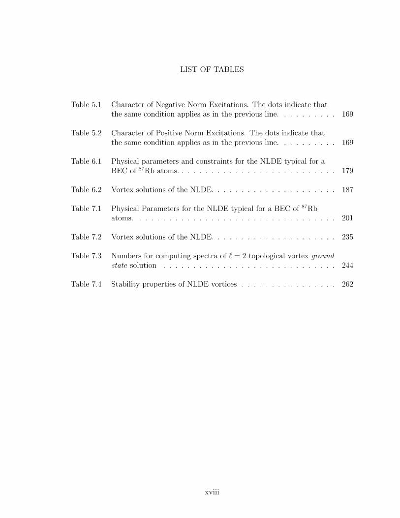
LIST OF TABLES . . . . . . . . . . . . . . . . . . . . . . . . . . . . . . . . . xviii

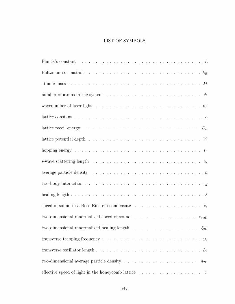
LIST OF SYMBOLS . . . . . . . . . . . . . . . . . . . . . . . . . . . . . . . . . xix

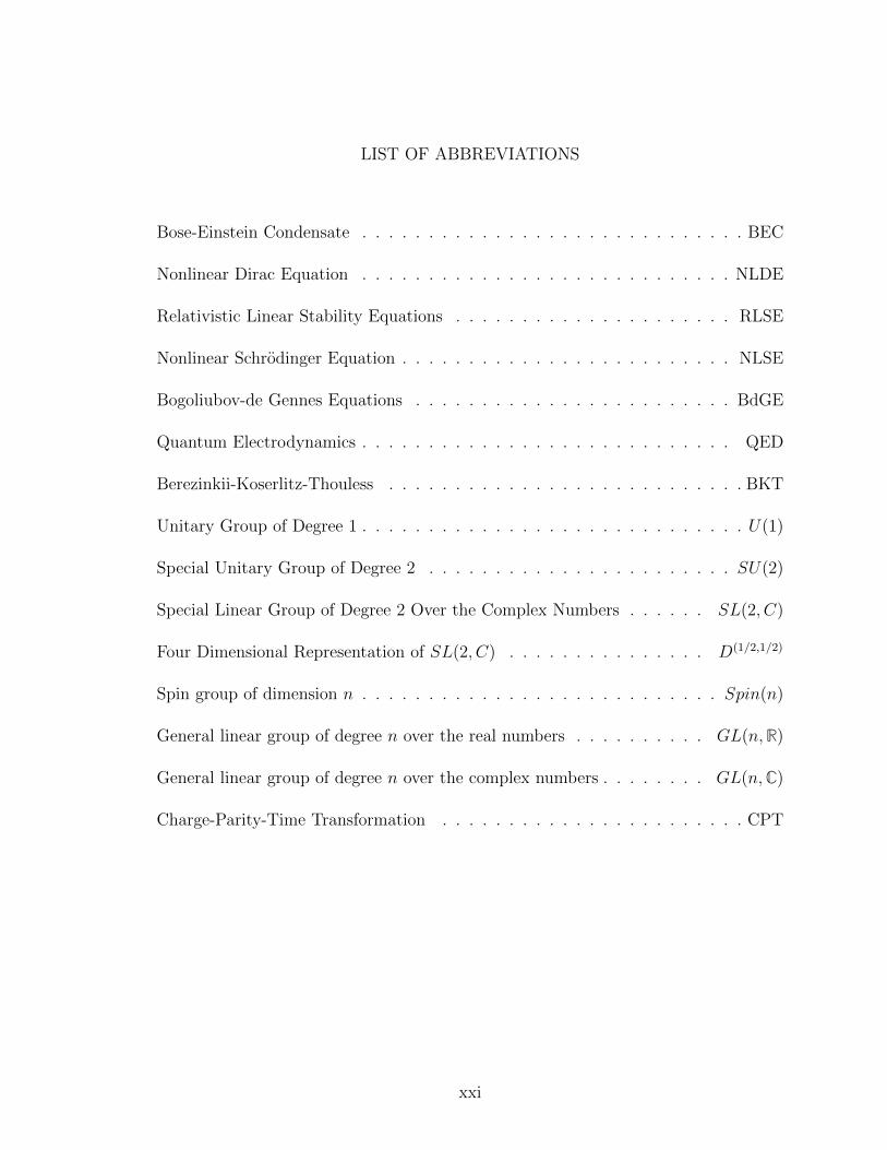
LIST OF ABBREVIATIONS . . . . . . . . . . . . . . . . . . . . . . . . . . . . xxi

ACKNOWLEDGMENTS . . . . . . . . . . . . . . . . . . . . . . . . . . . . . xxii

DEDICATION . . . . . . . . . . . . . . . . . . . . . . . . . . . . . . . . . . . xxiii

CHAPTER 1 INTRODUCTION . . . . . . . . . . . . . . . . . . . . . . . . . . . 1

1.1 Mean-field Theory and the Nonlinear Schrodinger Equation . . . . . . . . 4

1.2 Bogoliubov Theory . . . . . . . . . . . . . . . . . . . . . . . . . . . . . . 7

1.3 Reduction from Three Dimensions to Two Dimensions . . . . . . . . . . 9

1.4 Bose-Einstein Condensates in Two-Dimensional Optical Lattices . . . . 10

1.5 Cold Atom Interactions in Optical Lattices and Magnetic Traps . . . . 16

1.6 The Linear and Nonlinear Dirac Equations . . . . . . . . . . . . . . . . 18

1.7 Nonlinear Dirac Equations in Condensed Matter and Cold AtomicGases . . . . . . . . . . . . . . . . . . . . . . . . . . . . . . . . . . . . 25

1.8 Connections to Optics and Applied Mathematics . . . . . . . . . . . . . 27

1.9 Approximations and Constraints Involved in the Nonlinear DiracEquation . . . . . . . . . . . . . . . . . . . . . . . . . . . . . . . . . . . 28

1.10 Solution Methods for the Nonlinear Dirac Equation . . . . . . . . . . . 29

1.11 Overview of Thesis . . . . . . . . . . . . . . . . . . . . . . . . . . . . . 32

vii

CHAPTER 2 THE NONLINEAR DIRAC EQUATION IN BOSE-EINSTEINCONDENSATES: FOUNDATION AND SYMMETRIES . . . . . 37

2.1 Introduction . . . . . . . . . . . . . . . . . . . . . . . . . . . . . . . . . 38

2.2 The Nonlinear Dirac Equation . . . . . . . . . . . . . . . . . . . . . . . 40

2.2.1 Two-Component Spinor Form of the NLDE . . . . . . . . . . . 40

2.3 Maximally Compact Form of the NLDE . . . . . . . . . . . . . . . . . 50

2.4 Symmetries and Constraints . . . . . . . . . . . . . . . . . . . . . . . . 52

2.4.1 Locality . . . . . . . . . . . . . . . . . . . . . . . . . . . . . . . 53

2.4.2 Poincare Symmetry . . . . . . . . . . . . . . . . . . . . . . . . . 53

2.4.3 Hermiticity . . . . . . . . . . . . . . . . . . . . . . . . . . . . . 58

2.4.4 Current Conservation . . . . . . . . . . . . . . . . . . . . . . . . 58

2.4.5 Chiral Current . . . . . . . . . . . . . . . . . . . . . . . . . . . 59

2.4.6 Universality . . . . . . . . . . . . . . . . . . . . . . . . . . . . . 60

2.4.7 Discrete Symmetries . . . . . . . . . . . . . . . . . . . . . . . . 60

2.4.8 Parity . . . . . . . . . . . . . . . . . . . . . . . . . . . . . . . . 60

2.4.9 Charge Conjugation . . . . . . . . . . . . . . . . . . . . . . . . 61

2.4.10 Time Reversal . . . . . . . . . . . . . . . . . . . . . . . . . . . . 62

2.5 Discussion and Conclusions . . . . . . . . . . . . . . . . . . . . . . . . 63

CHAPTER 3 FOUNDATIONAL TOPICS IN THE NONLINEAR DIRACEQUATION: SPINOR FORMALISM, SPIN-STATISTICS,LAGRANGIAN ANALYSIS, AND REDUCTION TO THENONLINEAR SCHRODINGER EQUATION . . . . . . . . . . . 67

3.1 Introduction . . . . . . . . . . . . . . . . . . . . . . . . . . . . . . . . . 67

3.2 The Spin-Statistics Theorem and Honeycomb Lattice ElementaryExcitations . . . . . . . . . . . . . . . . . . . . . . . . . . . . . . . . . 68

viii

3.3 Spinor Formalism in the Dirac Equation . . . . . . . . . . . . . . . . . 72

3.3.1 Energy Versus Chiral Representation . . . . . . . . . . . . . . . 72

3.3.2 Lorentz Non-Covariance of the NLDE . . . . . . . . . . . . . . . 75

3.4 Lagrangian and Energy Functional of the Nonlinear Dirac Equation . . 79

3.4.1 Lagrangian Analysis . . . . . . . . . . . . . . . . . . . . . . . . 80

3.4.2 Energy Functional Analysis for Relativistic Vortices . . . . . . . 84

3.5 Reduction of the Time-Dependent NLDE to the Time-DependentNLSE with Correction Terms . . . . . . . . . . . . . . . . . . . . . . . 86

3.5.1 One-Dimensional Case . . . . . . . . . . . . . . . . . . . . . . . 87

3.5.2 Topological Solitons . . . . . . . . . . . . . . . . . . . . . . . . 88

3.5.3 Soliton Energy . . . . . . . . . . . . . . . . . . . . . . . . . . . 92

3.5.4 Nonlinear Sigma Model . . . . . . . . . . . . . . . . . . . . . . . 95

3.5.5 Two-Dimensional Case . . . . . . . . . . . . . . . . . . . . . . . 95

3.6 Conclusion . . . . . . . . . . . . . . . . . . . . . . . . . . . . . . . . . 100

CHAPTER 4 RELATIVISTIC LINEAR STABILITY EQUATIONS FORTHE NONLINEAR DIRAC EQUATION IN BOSE-EINSTEINCONDENSATES . . . . . . . . . . . . . . . . . . . . . . . . . . 103

4.1 Introduction . . . . . . . . . . . . . . . . . . . . . . . . . . . . . . . . 104

4.2 Derivation of the RLSE . . . . . . . . . . . . . . . . . . . . . . . . . . 107

4.3 Physical Parameters and Regimes . . . . . . . . . . . . . . . . . . . . 109

4.4 Uniformly Moving Condensate . . . . . . . . . . . . . . . . . . . . . . 110

4.5 Cherenkov Radiation . . . . . . . . . . . . . . . . . . . . . . . . . . . 112

4.6 Nonlinear Localized Modes . . . . . . . . . . . . . . . . . . . . . . . . 113

4.7 Localized Mode Stability . . . . . . . . . . . . . . . . . . . . . . . . . 115

ix

4.8 Conclusion . . . . . . . . . . . . . . . . . . . . . . . . . . . . . . . . . 119

CHAPTER 5 ESTABLISHING THE RELATIVISTIC LINEAR STABILITYEQUATIONS: MICROSCOPIC LATTICE DERIVATION,TRANSITION OF OPERATORS FROM LATTICE TOCONTINUUM, PROPERTIES OF SPINOR COHERENCEFACTORS AND INTERACTING GROUND STATE . . . . . 121

5.1 Introduction . . . . . . . . . . . . . . . . . . . . . . . . . . . . . . . . 121

5.2 Standard Theory for a Free Condensate . . . . . . . . . . . . . . . . . 121

5.3 Bogoliubov Theory for a Condensate at Dirac Point of a HoneycombLattice . . . . . . . . . . . . . . . . . . . . . . . . . . . . . . . . . . . 127

5.3.1 Transition of Operators Between Lattice and ContinuumLimits . . . . . . . . . . . . . . . . . . . . . . . . . . . . . . . 135

5.3.2 The Tight-Binding Limit Form of Bogoliubov Transformations 138

5.3.3 Derivation of the Constraint Equations for the Lattice:Relativistic Linear Stability Equations . . . . . . . . . . . . . 142

5.4 Calculation of RLSE Eigenvalues and Coherence Factors for aUniform Condensate . . . . . . . . . . . . . . . . . . . . . . . . . . . 145

5.5 Derivation of Condensate Phase Gradient Terms . . . . . . . . . . . . 146

5.6 Energy Eigenvalues . . . . . . . . . . . . . . . . . . . . . . . . . . . . 151

5.7 Limits of Quasi-Particle Energy . . . . . . . . . . . . . . . . . . . . . 154

5.7.1 Directional Behavior of the Energy . . . . . . . . . . . . . . . 155

5.8 Coherence Factors for Uniform Background . . . . . . . . . . . . . . . 158

5.9 Interacting Ground-State . . . . . . . . . . . . . . . . . . . . . . . . . 162

5.10 General Properties of the RLSE, Quasi-Particle States, and Energies . 163

5.11 Symmetries of the RLSE . . . . . . . . . . . . . . . . . . . . . . . . . 164

5.12 Normalization of Quasi-Particle States . . . . . . . . . . . . . . . . . 165

x

5.13 Positive and Negative Energy States: Lattice Versus InteractionEffects . . . . . . . . . . . . . . . . . . . . . . . . . . . . . . . . . . . 167

5.14 Analytical Solutions of the RLSE for Arbitrary Vortex Background . 170

5.15 Conclusion . . . . . . . . . . . . . . . . . . . . . . . . . . . . . . . . . 175

CHAPTER 6 THE NONLINEAR DIRAC EQUATION: RELATIVISTICVORTICES AND EXPERIMENTAL REALIZATION INBOSE-EINSTEIN CONDENSATES . . . . . . . . . . . . . . . 177

6.1 Main Text . . . . . . . . . . . . . . . . . . . . . . . . . . . . . . . . . 178

6.2 Supplementary Materials . . . . . . . . . . . . . . . . . . . . . . . . . 187

CHAPTER 7 THE NONLINEAR DIRAC EQUATION: METASTABLERELATIVISTIC VORTICES IN A BOSE-EINSTEINCONDENSATE . . . . . . . . . . . . . . . . . . . . . . . . . . 193

7.1 Introduction . . . . . . . . . . . . . . . . . . . . . . . . . . . . . . . . 194

7.2 Experimental Realization of the NLDE . . . . . . . . . . . . . . . . . 198

7.2.1 Renormalized Parameters and Physical Constraints . . . . . . 200

7.2.2 Transition from 3D to 2D NLSE . . . . . . . . . . . . . . . . . 200

7.2.3 Derivation of NLDE from 2D NLSE. . . . . . . . . . . . . . . 202

7.2.3.1 Normalization Condition. . . . . . . . . . . . . . . . 203

7.2.3.2 Renormalized Atomic Interaction. . . . . . . . . . . . 204

7.2.3.3 Natural Parameters of the NLDE . . . . . . . . . . . 204

7.2.4 Physical Constraints . . . . . . . . . . . . . . . . . . . . . . . 205

7.2.5 Lattice Construction . . . . . . . . . . . . . . . . . . . . . . . 208

7.2.6 Preparing a BEC at a Dirac Point . . . . . . . . . . . . . . . . 209

7.2.7 Coherent Transfer Between Sublattices . . . . . . . . . . . . . 212

7.2.8 Creation of Vortices . . . . . . . . . . . . . . . . . . . . . . . . 215

xi

7.2.9 Coherent Transfer Between Dirac Points by Bragg Scattering . 217

7.3 Vortex Solutions of the NLDE . . . . . . . . . . . . . . . . . . . . . . 218

7.3.1 Asymptotic Bessel Solutions for Large Phase Winding . . . . 220

7.3.2 Numerical Shooting Method for Vortices with Arbitrary PhaseWinding and Chemical Potential . . . . . . . . . . . . . . . . 222

7.3.3 Algebraic Solutions for Zero Chemical Potential and PhaseWinding Greater than One . . . . . . . . . . . . . . . . . . . . 224

7.3.4 Algebraic Solutions for Zero and Unit Phase Winding . . . . . 227

7.3.5 Ring-Vortex/Soliton. . . . . . . . . . . . . . . . . . . . . . . . 227

7.3.6 Vortex/Soliton. . . . . . . . . . . . . . . . . . . . . . . . . . . 229

7.3.7 Skyrmion Solutions . . . . . . . . . . . . . . . . . . . . . . . . 230

7.3.8 Anderson-Toulouse Skyrmions . . . . . . . . . . . . . . . . . . 232

7.3.9 Mermin-Ho Skyrmions . . . . . . . . . . . . . . . . . . . . . . 232

7.3.10 Half-Quantum Vortices . . . . . . . . . . . . . . . . . . . . . . 233

7.4 Spectra for Relativistic Vortices . . . . . . . . . . . . . . . . . . . . . 235

7.4.1 Ground State and Radial Excitations of Unconfined Vortices . 236

7.4.2 Solutions for Unit Phase Winding . . . . . . . . . . . . . . . . 238

7.4.3 Solutions for Phase Winding Greater than One . . . . . . . . 239

7.4.4 Special Case of Zero Chemical Potential: LocalizedRing-Vortices . . . . . . . . . . . . . . . . . . . . . . . . . . . 240

7.4.5 Discrete Eigenvalue Spectra for Vortices in a Weak HarmonicTrap . . . . . . . . . . . . . . . . . . . . . . . . . . . . . . . . 241

7.5 Relativistic Linear Stability Equations . . . . . . . . . . . . . . . . . 243

7.5.1 Derivation . . . . . . . . . . . . . . . . . . . . . . . . . . . . . 245

xii

7.5.2 First Method - Tight-Binding Limit Followed byDiagonalization of the Quasi-Particle Hamiltonian . . . . . . . 248

7.5.3 Second Method - Diagonalize the Quasi-Particle Hamiltonianthen Impose Tight-Binding . . . . . . . . . . . . . . . . . . . . 253

7.5.4 Proof of NLDE Limit to NLSE . . . . . . . . . . . . . . . . . 255

7.5.5 Proof of RLSE limit to BdGE . . . . . . . . . . . . . . . . . . 257

7.6 Stability of Vortex Solutions . . . . . . . . . . . . . . . . . . . . . . . 258

7.6.1 Solving the RLSE . . . . . . . . . . . . . . . . . . . . . . . . . 259

7.6.2 Computing Vortex Lifetimes . . . . . . . . . . . . . . . . . . . 261

7.7 Conclusion . . . . . . . . . . . . . . . . . . . . . . . . . . . . . . . . . 264

7.8 Appendix A: Convergence of Numerical Solutions of the NLDE andRLSE . . . . . . . . . . . . . . . . . . . . . . . . . . . . . . . . . . . 266

CHAPTER 8 THE NONLINEAR DIRAC EQUATION: RELATIVISTICSOLITONS AND MASS GAPS . . . . . . . . . . . . . . . . . . 269

8.1 Introduction . . . . . . . . . . . . . . . . . . . . . . . . . . . . . . . . 270

8.2 Soliton Solutions of the NLDE . . . . . . . . . . . . . . . . . . . . . . 273

8.3 Bright Soliton Train . . . . . . . . . . . . . . . . . . . . . . . . . . . 275

8.3.1 Soliton Expansion and Conserved Charges . . . . . . . . . . . 277

8.3.2 Numerical Solitons . . . . . . . . . . . . . . . . . . . . . . . . 280

8.4 Mass Gaps for the NLDE . . . . . . . . . . . . . . . . . . . . . . . . . 281

8.4.1 General Embedded and Gap Solitons . . . . . . . . . . . . . . 283

8.4.2 Mapping to the Integrable Thirring Model . . . . . . . . . . . 285

8.4.3 Derivation of the Mapping . . . . . . . . . . . . . . . . . . . . 285

8.4.4 NLDE Gap Solitons from the Thirring Mapping . . . . . . . . 287

xiii

8.4.5 Implications of the Mapping: Integrability of a RelativisticSubspace of Solutions . . . . . . . . . . . . . . . . . . . . . . . 289

8.5 Stability of Soliton Solutions . . . . . . . . . . . . . . . . . . . . . . . 290

8.5.1 Linear Eigenvalues . . . . . . . . . . . . . . . . . . . . . . . . 291

8.5.2 Computing the Line Soliton Lifetime . . . . . . . . . . . . . . 292

8.6 Soliton Spectra in a Harmonic Trap . . . . . . . . . . . . . . . . . . . 293

8.6.1 Quantized Excitations . . . . . . . . . . . . . . . . . . . . . . 294

8.6.2 Eigenvalue Spectra and Macroscopic Klein-Tunneling . . . . . 295

8.7 Conclusion . . . . . . . . . . . . . . . . . . . . . . . . . . . . . . . . . 301

8.8 Appendix A: Continuous Spectrum of the NLDE . . . . . . . . . . . 302

8.8.1 Four-Spinor Spectrum . . . . . . . . . . . . . . . . . . . . . . 302

8.8.2 Resonances at k = 0 . . . . . . . . . . . . . . . . . . . . . . . 304

8.8.3 Two-Spinor Spectrum . . . . . . . . . . . . . . . . . . . . . . 304

8.8.4 Static Solutions for Zero Chemical Potential . . . . . . . . . . 305

8.8.5 Resonances at k = 0 . . . . . . . . . . . . . . . . . . . . . . . 305

CHAPTER 9 EFFECTIVE QUANTUM FIELD THEORY FOR BOSONSIN THE HONEYCOMB LATTICE . . . . . . . . . . . . . . . 307

9.1 Introduction . . . . . . . . . . . . . . . . . . . . . . . . . . . . . . . . 308

9.2 Microscopic Derivation of the Many-body Hamiltonian for Bosons ina Honeycomb Lattice . . . . . . . . . . . . . . . . . . . . . . . . . . . 308

9.2.1 First-Order Nearest-Neighbor Hopping . . . . . . . . . . . . . 308

9.2.2 Second-Order Nearest-Neighbor Hopping Correction . . . . . . 313

9.3 Continuum Quantum Field Theory . . . . . . . . . . . . . . . . . . . 319

9.4 Conclusion . . . . . . . . . . . . . . . . . . . . . . . . . . . . . . . . . 326

xiv

CHAPTER 10CONCLUSIONS AND OUTLOOK . . . . . . . . . . . . . . . . 329

REFERENCES CITED . . . . . . . . . . . . . . . . . . . . . . . . . . . . . . 335

xv

LIST OF FIGURES

Figure 2.1 Characterization of a honeycomb lattice. . . . . . . . . . . . . . . . 41

Figure 4.1 The honeycomb optical lattice . . . . . . . . . . . . . . . . . . . . 106

Figure 4.2 Localized solutions of the NLDE . . . . . . . . . . . . . . . . . . . 114

Figure 4.3 Lowest quasi-particle excitation for the vortex/solitonconfiguration. . . . . . . . . . . . . . . . . . . . . . . . . . . . . . 116

Figure 6.1 Bragg scattering in a spin-dependent honeycomb lattice. . . . . . 181

Figure 6.2 Coherent transfer between sublattices A and B . . . . . . . . . . . 182

Figure 6.3 Relativistic vortices. . . . . . . . . . . . . . . . . . . . . . . . . . . 183

Figure 7.1 The honeycomb optical lattice . . . . . . . . . . . . . . . . . . . . 199

Figure 7.2 Convergence of numerical vortex for ` = 2 . . . . . . . . . . . . . 224

Figure 7.3 Connection of ring-vortex solution to free particle Bessel solution . 225

Figure 7.4 Phase and density for the Bessel topological vortex for ` = 4 . . . 226

Figure 7.5 Phase and density for the ` = 4 numerical topological vortex . . . 227

Figure 7.6 NLDE vortex radial solutions . . . . . . . . . . . . . . . . . . . . 228

Figure 7.7 Phase and density for the ` = 2 ring-vortex . . . . . . . . . . . . . 229

Figure 7.8 Phase and density for the ` = 1 ring-vortex/soliton . . . . . . . . 230

Figure 7.9 Phase and density for the ` = 1 vortex/soliton . . . . . . . . . . . 232

Figure 7.10 Phase and density for the ` = 1 Anderson-Toulouse skyrmion . . . 233

Figure 7.11 NLDE vortex radial solutions . . . . . . . . . . . . . . . . . . . . 234

Figure 7.12 Phase and density for the ` = 1 Mermin-Ho skyrmion . . . . . . . 236

xvi

Figure 7.13 Phase and density for the half-quantum vortex solutions . . . . . 237

Figure 7.14 Radial excited states for ` = 1 . . . . . . . . . . . . . . . . . . . . 238

Figure 7.15 Radial profiles for ` = 1 flat solution . . . . . . . . . . . . . . . . . 240

Figure 7.16 Radial ring-vortex states for ` = 2 topological solution in theharmonic trap . . . . . . . . . . . . . . . . . . . . . . . . . . . . . 242

Figure 7.17 Anomalous mode frequencies for the vortex/soliton . . . . . . . . 260

Figure 7.18 Imaginary parts of the five lowest quasi-particle excitationenergies for the ring/vortex solution . . . . . . . . . . . . . . . . . 261

Figure 7.19 Convergence of RLSE for the vortex/soliton . . . . . . . . . . . . 267

Figure 7.20 Convergence of the l = 2 ring-vortex solution . . . . . . . . . . . . 267

Figure 8.4 Numerical solutions of the NLDE . . . . . . . . . . . . . . . . . . 282

Figure 8.5 Soliton densities . . . . . . . . . . . . . . . . . . . . . . . . . . . . 283

Figure 8.6 Real and imaginary parts of Thirring solutions . . . . . . . . . . . 289

Figure 8.7 Numerical shooting results for the line soliton . . . . . . . . . . . 295

Figure 8.8 Numerical shooting results for the line soliton in a harmonic trap 296

Figure 8.9 Ground state of the line soliton in a trap with soft boundary . . . 299

Figure 8.10 Discrete spectra of the line soliton in a harmonic trap . . . . . . . 300

xvii

LIST OF TABLES

Table 5.1 Character of Negative Norm Excitations. The dots indicate thatthe same condition applies as in the previous line. . . . . . . . . . 169

Table 5.2 Character of Positive Norm Excitations. The dots indicate thatthe same condition applies as in the previous line. . . . . . . . . . 169

Table 6.1 Physical parameters and constraints for the NLDE typical for aBEC of 87Rb atoms. . . . . . . . . . . . . . . . . . . . . . . . . . . 179

Table 6.2 Vortex solutions of the NLDE. . . . . . . . . . . . . . . . . . . . . 187

Table 7.1 Physical Parameters for the NLDE typical for a BEC of 87Rbatoms. . . . . . . . . . . . . . . . . . . . . . . . . . . . . . . . . . 201

Table 7.2 Vortex solutions of the NLDE. . . . . . . . . . . . . . . . . . . . . 235

Table 7.3 Numbers for computing spectra of ` = 2 topological vortex groundstate solution . . . . . . . . . . . . . . . . . . . . . . . . . . . . . 244

Table 7.4 Stability properties of NLDE vortices . . . . . . . . . . . . . . . . 262

xviii

LIST OF SYMBOLS

Planck’s constant . . . . . . . . . . . . . . . . . . . . . . . . . . . . . . . . . . . ~

Boltzmann’s constant . . . . . . . . . . . . . . . . . . . . . . . . . . . . . . . . kB

atomic mass . . . . . . . . . . . . . . . . . . . . . . . . . . . . . . . . . . . . . . M

number of atoms in the system . . . . . . . . . . . . . . . . . . . . . . . . . . . N

wavenumber of laser light . . . . . . . . . . . . . . . . . . . . . . . . . . . . . . kL

lattice constant . . . . . . . . . . . . . . . . . . . . . . . . . . . . . . . . . . . . . a

lattice recoil energy . . . . . . . . . . . . . . . . . . . . . . . . . . . . . . . . . . ER

lattice potential depth . . . . . . . . . . . . . . . . . . . . . . . . . . . . . . . . V0

hopping energy . . . . . . . . . . . . . . . . . . . . . . . . . . . . . . . . . . . . th

s-wave scattering length . . . . . . . . . . . . . . . . . . . . . . . . . . . . . . . as

average particle density . . . . . . . . . . . . . . . . . . . . . . . . . . . . . . . . n

two-body interaction . . . . . . . . . . . . . . . . . . . . . . . . . . . . . . . . . . g

healing length . . . . . . . . . . . . . . . . . . . . . . . . . . . . . . . . . . . . . . ξ

speed of sound in a Bose-Einstein condensate . . . . . . . . . . . . . . . . . . . cs

two-dimensional renormalized speed of sound . . . . . . . . . . . . . . . . . . cs,2D

two-dimensional renormalized healing length . . . . . . . . . . . . . . . . . . . . ξ2D

transverse trapping frequency . . . . . . . . . . . . . . . . . . . . . . . . . . . . ωz

transverse oscillator length . . . . . . . . . . . . . . . . . . . . . . . . . . . . . . Lz

two-dimensional average particle density . . . . . . . . . . . . . . . . . . . . . n2D

effective speed of light in the honeycomb lattice . . . . . . . . . . . . . . . . . . cl

xix

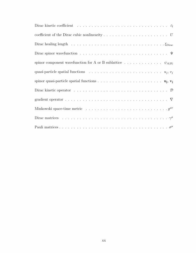
Dirac kinetic coefficient . . . . . . . . . . . . . . . . . . . . . . . . . . . . . . . cl

coefficient of the Dirac cubic nonlinearity . . . . . . . . . . . . . . . . . . . . . . U

Dirac healing length . . . . . . . . . . . . . . . . . . . . . . . . . . . . . . . . ξDirac

Dirac spinor wavefunction . . . . . . . . . . . . . . . . . . . . . . . . . . . . . . Ψ

spinor component wavefunction for A or B sublattice . . . . . . . . . . . . . ψA(B)

quasi-particle spatial functions . . . . . . . . . . . . . . . . . . . . . . . . . uj, vj

spinor quasi-particle spatial functions . . . . . . . . . . . . . . . . . . . . . . uj, vj

Dirac kinetic operator . . . . . . . . . . . . . . . . . . . . . . . . . . . . . . . . D

gradient operator . . . . . . . . . . . . . . . . . . . . . . . . . . . . . . . . . . . ∇

Minkowski space-time metric . . . . . . . . . . . . . . . . . . . . . . . . . . . . gµν

Dirac matrices . . . . . . . . . . . . . . . . . . . . . . . . . . . . . . . . . . . . γµ

Pauli matrices . . . . . . . . . . . . . . . . . . . . . . . . . . . . . . . . . . . . . σµ

xx

LIST OF ABBREVIATIONS

Bose-Einstein Condensate . . . . . . . . . . . . . . . . . . . . . . . . . . . . . BEC

Nonlinear Dirac Equation . . . . . . . . . . . . . . . . . . . . . . . . . . . . NLDE

Relativistic Linear Stability Equations . . . . . . . . . . . . . . . . . . . . . RLSE

Nonlinear Schrodinger Equation . . . . . . . . . . . . . . . . . . . . . . . . . NLSE

Bogoliubov-de Gennes Equations . . . . . . . . . . . . . . . . . . . . . . . . BdGE

Quantum Electrodynamics . . . . . . . . . . . . . . . . . . . . . . . . . . . . QED

Berezinkii-Koserlitz-Thouless . . . . . . . . . . . . . . . . . . . . . . . . . . . BKT

Unitary Group of Degree 1 . . . . . . . . . . . . . . . . . . . . . . . . . . . . . U(1)

Special Unitary Group of Degree 2 . . . . . . . . . . . . . . . . . . . . . . . SU(2)

Special Linear Group of Degree 2 Over the Complex Numbers . . . . . . SL(2, C)

Four Dimensional Representation of SL(2, C) . . . . . . . . . . . . . . . D(1/2,1/2)

Spin group of dimension n . . . . . . . . . . . . . . . . . . . . . . . . . . . Spin(n)

General linear group of degree n over the real numbers . . . . . . . . . . GL(n,R)

General linear group of degree n over the complex numbers . . . . . . . . GL(n,C)

Charge-Parity-Time Transformation . . . . . . . . . . . . . . . . . . . . . . . CPT

xxi

ACKNOWLEDGMENTS

First, I would like to thank my advisor Lincoln Carr for his enthusiasm, insight,

creative fervor, and contagious adventurous spirit which have supplied me with hope

and inspiration during the long hours deriving equations. Though he has been a

helpful guide to me in terms of the technical details of my work, it is the positive

energy that surrounds him that has been an indispensable component to my success.

I am grateful for his choice of research project which somehow was a perfect fit to

my experience and personal inclinations. I attribute our first meeting to fate but

subsequent direction in my research to Lincoln’s depth and breadth of knowledge of

physics.

I want to acknowledge Ken O’Hara for contributing his technical ability and in-

tuitive insight to our project. Working with him has increased my knowledge and

appreciation of the experimental side of cold atoms. To observe his thought process

during the evolution of our work on the nonlinear Dirac equation has been truly

enlightening.

I would also like to acknowledge the help and support of Michael Wall. He is not

only an immensely gifted physicist, but also a person of the heart for whom I have

great respect. The discussions we have had over the past few years continue to inspire

me and fill me with new ideas. I have enjoyed the time spent with other students at

CSM as well. Majed Alotaibi, Erman Bekaroglu, Miguel Angel Garcıa March, Scott

Strong, Alex Yuffa, Rahman Rezwanur, Tori Semi and others who have enriched my

time at CSM.

xxii

I dedicate this thesis to my daughter Alyssa and to my mother and father, my

brothers and sister, and to my friends. I also dedicate it to my uncle and

grandmother. They are in my thoughts and in my heart during every moment of my

work.

“ Look for the stars, you’ll say that there are none;

Look up a second time, and, one by one,

You mark them twinkling out with silvery light,

And wonder how they could elude the sight! ”

-William Wordsworth

xxiii

CHAPTER 1

INTRODUCTION

Since the earliest experiments with laser cooling of atoms and in particular with

the creation [1–3] of the first Bose-Einstein condensate (BEC),1 we have seen an

explosion of theoretical and experimental work in the field of cold atomic gases [4–18].

Contributions have come from a diverse array of fields in theoretical and experimental

physics, physical chemistry, and applied mathematics [19]. Major areas of impact

include nonlinear optics [20–22], physics of the Bose-Einstein condensate to Bardeen-

Cooper-Schrieffer superconductivity crossover (BEC-BCS) [23–25], and the dynamics

of quantum vortices [26–29]. Advances in the engineering of trapped cold atoms

in optical lattices have extended our reach into such exotic aspects of matter as

topological insulators, spintronics, and meta-materials. On the mathematics side, our

understanding of nonlinear partial differential equations, rooted in mathematics as

well as in nonlinear physics, has been vigorously stimulated by the increased interest

in BECs [30–32]. As a product of the strong interdisciplinary nature of these topics

and the increased ability to manipulate atoms, a new unifying theme is gradually

emerging. This is the study of condensed matter and particle physics analogs or

simply quantum analogs : the modeling of foundational problems in physics using

constructions of cold atomic gases [8, 33, 34].

Several developments have made it easier to explore these analogies. For example,

with the construction of optical lattices we are now able to model a wide range of

condensed matter systems [5, 8]. We can control impurities to a degree not possible

in experiments with ordinary crystals. Precise Feshbach resonance tuning allows us

1The 2001 Nobel prize for physics was awarded for the discovery of the BEC to Carl Wiemanand Eric Cornell at the University of Colorado at Boulder NIST-JILA lab, and to Wolfgang Ketterleat Massachusetts Institute of Technology.

1

to control the sign, strength, and symmetry of atomic interactions [35]. A variety of

periodic systems of ultracold bosonic [36] or fermionic [37] atoms and molecules have

been constructed via optical lattices. Spinor condensates which rely on the hyperfine

structure of alkali atoms to create a macroscopic pseudospin, are particularly relevant

to our work and provide a practical method for constructing multi-component BECs

with interesting topologies [38–44]. Such condensates were first realized experimen-

tally for the upper and lower hyperfine states of 87Rb atoms [9, 45], and soon followed

for the case of three hyperfine orientations mF = 1, 0,−1 for the F = 1 ground state

of sodium [10, 46]. In particular, for the case of 87Rb, the angular momentum of

the nucleus, I = 3/2, and the outer electron, J = 1/2, allow for two possible values

of the total angular momentum F = 1, 2. When the various hyperfine states la-

beled by the z-components mF are weakly coupled, this gives rise to interpenetrating

superfluids [45, 47].

Our work on BECs in honeycomb lattices connects to important contemporary

topics in fundamental and applied physics. In 2004, the first stable monolayer of

graphite, graphene, was realized in the laboratory [48–51].2 The creation of graphene

is an exciting new development for two reasons. First, from a technological standpoint

its electronic spectrum allows for high mobility of charge carriers, making graphene a

good candidate for future replacement of silicon in computing technology. Moreover,

at low energies, graphene’s honeycomb lattice structure and linear dispersion means

that charge carriers are chiral and propagate as massless Dirac fermions at an effective

speed of light ceff = vF ' c/300, where vF is the Fermi velocity. In contrast, we show

that a BEC in a honeycomb lattice exhibits relativistic Dirac physics at a velocity 10

orders of magnitude slower than the speed of light. This gives us tabletop access to

slow relativistic quantum phenomena [52].

2The 2010 Nobel prize for physics was awarded to Andre Geim and Konstantin Novoselov at theUniversity of Manchester for their work in isolating flakes of graphene.

2

The problems which we explore in this thesis were inspired by the condensed

matter/particle physics connection and involve theoretical studies beginning with

the optical lattice counterpart of graphene in which ultracold bosonic atoms replace

electrons, but retaining graphene’s characteristic honeycomb lattice. We obtain the

same result as that found in the graphene literature [53, 54], namely that the bipartite

structure of the lattice induces a chiral structure on the order parameter as well as

reproducing the linear Dirac dispersion [52]. This similarity to graphene is purely

due to the honeycomb lattice geometry. However, a significant difference in our case

is that, by including contact interactions for bosons, we have obtained a nonlinear

Dirac equation (NLDE) for the BEC order parameter.

Our model is an ideal starting point for bridging condensed matter systems to var-

ious phenomenological models where Dirac fermions can be strongly coupled to other

fields or to themselves, as well as gaining a deeper understanding of the fundamental

distinction between bosons and fermions. Our studies take place specifically within

the context of soliton and vortex solutions of the NLDE. Nonlinear Dirac theories

have been used to describe such exotic phenomena as low energy fermions at the

intersections of D-branes in string theory using Jona-Lasinio and Gross-Neveu mod-

els [55, 56]. These are phenomenological QCD models in that asymptotic freedom and

dynamical mass generation are generic features. Other examples include BCS theory

with mediating phonons integrated out, weak interactions in the Standard Model and

the study of the renormalization of quantum field theories in the large N limit.

In this introduction, we present several topics which provide important back-

ground material key to understanding and motivating the work in this thesis. In

Sec. 1.1, we review the basic idea behind mean-field theory, a paradigm which is cen-

tral to the NLDE. In particular, we review the nonlinear Schrodinger equation which

is fundamentally connected to the NLDE. Bogoliubov theory is another foundational

topic which underlies our work. In Sec. 1.2, we review the motivating assumptions

3

and physical results obtained through Bogoliubov’s method. The physical results

presented in this thesis pertain to 2D systems, or to quasi-1D systems. In Sec. 1.3 we

explain how dimensional reduction takes place from both the physical as well math-

ematical perspective. In Sec. 1.4, we review BECs in 2D systems through concepts

such as superfluidity and the BKT transition, as well as concepts fundamental to

optical lattice cold atoms, such as the Bose-Hubbard model. In Sec. 1.5, we discuss

interactions of cold atoms in magnetic fields and optical lattices. In Sec. 1.6, we

review the basics of Dirac theory and present some history and motivation behind

the nonlinear Dirac equation. In Sec. 1.7, we provide a context for the NLDE as it

occurs in optical lattices. in Sec. 1.8, we look at some contemporary fields of research

in optics and applied mathematics where the NLDE plays a key role. In Sec. 1.9,

the approximations and constraints needed to observe NLDE physics are discussed.

Finally, methods for obtaining vortex and soliton solutions of the NLDE are outlined

in Sec. 1.10.

1.1 Mean-field Theory and the Nonlinear Schrodinger Equation

The standard approach to mean-field theory was originally developed by Bogoli-

ubov in 1947, and then Gross and Pitaevskii (1961) [57–59]. A succinct explanation

is provided in Ref. [27]. The mean-field approach provides a useful paradigm for

computing the properties of a Bose gas when most of the particles are in the ground

state of the system, i.e, under BEC conditions with minimal depletion. To develop

mean-field theory for bosons, one starts from the full many-body Hamiltonian for

interacting bosons under the approximation of contact interactions, appropriate to

low energy s-wave scattering,

H =

∫dr ψ†(r)

[− ~2

2m∇2 + Vext(r)

]ψ(r) +

1

2

4π~2asm

∫dr ψ†(r)ψ†(r)ψ(r)ψ(r) , (1.1)

4

where ψ† (ψ) represents the field operator which creates (destroys) a particle at the

spatial point r, Vext is an external potential, and as and m are the s-wave scattering

length and mass for the constituent bosons. The field operator in Eq. (1.1) pertains

to bosonic atoms, so that the bosonic commutation relations apply,

[ψ(r), ψ†(r′)

]= δ(r− r′). (1.2)

We will see that in our work Vext is the periodic lattice potential throughout the thesis,

plus an additional harmonic trap in Chapters 7 and 8. The time evolution of the field

operator ψ is obtained according to the Heisenberg prescription i~ ∂ψ/∂t = [ψ, H],

whereby one obtains the equation of motion

i~∂

∂tψ(r, t) =

[− ~2

2m∇2 + Vext(r)

]ψ(r, t) +

4π~2asm

ψ†(r, t)ψ(r, t) ψ(r, t) , (1.3)

where we have used the bosonic field commutation relations for ψ in Eq. (1.2). The

field operator is then expressed as a sum of condensate and noncondensate particle

operators

ψ(r, t) = Ψ(r, t) + ϕ(r, t) , (1.4)

where Ψ represents the condensate and ϕ the non-condensate part.

At this point one assumes a dilute Bose gas so that most of the particles are in

the ground state condensate, i.e., that N − N0 N , where N is the total number

of particles and N0 is the number of particles in the condensate. Assuming weak in-

teractions, the condensate can then be approximately represented by a classical field

instead of a quantum operator due to U(1) symmetry breaking and an approximate

coherent state.3 Thus we can replace the operator Ψ(r, t) by a complex scalar func-

tion, namely the expectation value Ψ(r, t) ≡ 〈Ψ(r, t)〉. Taking the expectation value

3Here we do not consider a perfect coherent state as such states do not conserve particle num-ber [60].

5

of Eq. (1.3) and using the mean-field decomposition [61] for products of operators

〈. . . ψ† . . . ψ . . . 〉 = . . . 〈ψ†〉 . . . 〈ψ〉 . . . , Eq. (1.3) becomes

i~∂

∂tΨ(r, t) =

[− ~2

2m∇2 + Vext(r)

]Ψ(r, t) +

4π~2asm

|Ψ(r, t)|2 Ψ(r, t) . (1.5)

Equation (1.5) is the Gross-Pitaevskii equation (GPE), or nonlinear Schrodinger equa-

tion (NLSE) [58, 59] for the evolution of the complex function Ψ(r, t) with cubic

nonlinearity, interacting with the external potential Vext(r).

When dealing with excitations of a Bose gas in the ground state of a lattice, we

require a discrete version of Eq. (1.5), the discrete nonlinear Schrodinger (DNLS)

equation [62]. The nature of the DNLS can be pedagogically demonstrated for the

case where Vext(x) = Vlat(x) is a one-dimensional periodic lattice potential, and for the

moment we ignore the other two spatial dimensions y, z. The mean-field wavefunction

can then be expanded in terms of Bloch functions, Ψk,α(x) = eikxukα(x), where k is

the Bloch wavevector and α refers to the energy band, or alternatively in terms of

Wannier functions which are localized functions around the lattice sites. Defined

explicitly in terms of Bloch functions, the Wannier functions which we take to be real

are

wnα(x− nL) =

√L

2π

∫ π/L

−π/LdkΨkα(x)e−inkL , (1.6)

where L is the period of the potential and n refers to the nth lattice position. These

functions form a complete orthonormal set so that any solution of the NLSE can

be expressed as Ψ(x, t) =∑

nα cnα(t)wnα(x). Upon substitution into the NLSE,

multiplying through by wnα and integrating over x gives the result

6

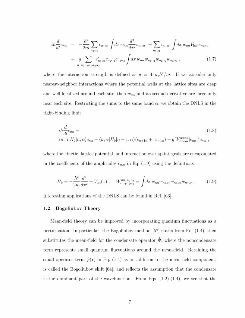
i~d

dtcnα = − ~2

2m

∑n1α1

cn1α1

∫dxwnα

d2

dx2wn1α1 +

∑n1α1

cn1α1

∫dxwnαVlatwn1α1

+ g∑

n1n2n3α1α2α3

c∗n1α1cn2α2cn3α3

∫dxwnαwn1α1wn2α2wn3α3 , (1.7)

where the interaction strength is defined as g ≡ 4πas~2/m. If we consider only

nearest-neighbor interactions where the potential wells at the lattice sites are deep

and well localized around each site, then wnα and its second derivative are large only

near each site. Restricting the sums to the same band α, we obtain the DNLS in the

tight-binding limit,

i~d

dtcnα = (1.8)

〈n, α|H0|n, α〉cnα + 〈n, α|H0|n+ 1, α〉(cn+1α + cn−1α) + gW nnnnαααα|cnα|2cnα ,

where the kinetic, lattice potential, and interaction overlap integrals are encapsulated

in the coefficients of the amplitudes cn,α in Eq. (1.9) using the definitions

H0 = − ~2

2m

d2

dx2+ Vlat(x) , W nn1n2n3

αα1α2α3=

∫dxwnαwn1α1wn2α2wn3α3 . (1.9)

Interesting applications of the DNLS can be found in Ref. [63].

1.2 Bogoliubov Theory

Mean-field theory can be improved by incorporating quantum fluctuations as a

perturbation. In particular, the Bogoliubov method [57] starts from Eq. (1.4), then

substitutes the mean-field for the condensate operator Ψ, where the noncondensate

term represents small quantum fluctuations around the mean-field. Retaining the

small operator term ϕ(r) in Eq. (1.4) as an addition to the mean-field component,

is called the Bogoliubov shift [64], and reflects the assumption that the condensate

is the dominant part of the wavefunction. From Eqs. (1.2)-(1.4), we see that the

7

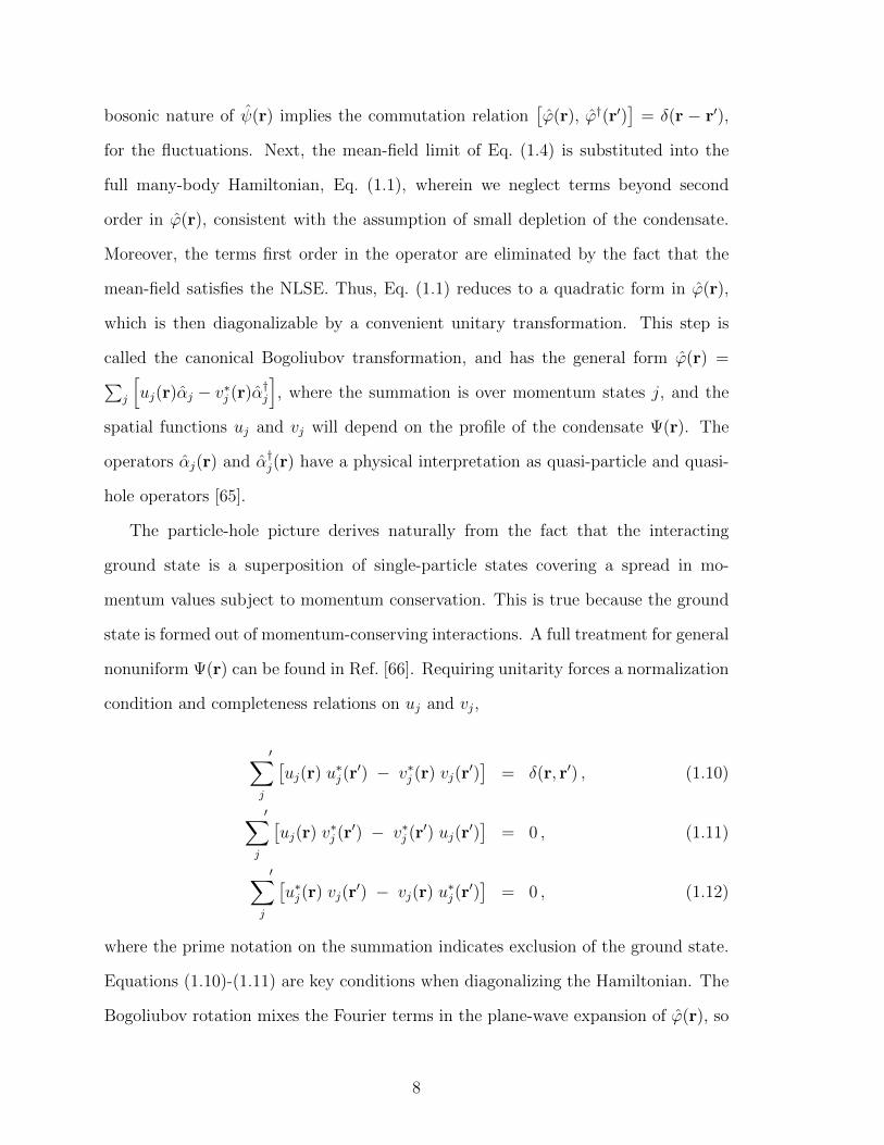
bosonic nature of ψ(r) implies the commutation relation[ϕ(r), ϕ†(r′)

]= δ(r − r′),

for the fluctuations. Next, the mean-field limit of Eq. (1.4) is substituted into the

full many-body Hamiltonian, Eq. (1.1), wherein we neglect terms beyond second

order in ϕ(r), consistent with the assumption of small depletion of the condensate.

Moreover, the terms first order in the operator are eliminated by the fact that the

mean-field satisfies the NLSE. Thus, Eq. (1.1) reduces to a quadratic form in ϕ(r),

which is then diagonalizable by a convenient unitary transformation. This step is

called the canonical Bogoliubov transformation, and has the general form ϕ(r) =∑j

[uj(r)αj − v∗j (r)α†j

], where the summation is over momentum states j, and the

spatial functions uj and vj will depend on the profile of the condensate Ψ(r). The

operators αj(r) and α†j(r) have a physical interpretation as quasi-particle and quasi-

hole operators [65].

The particle-hole picture derives naturally from the fact that the interacting

ground state is a superposition of single-particle states covering a spread in mo-

mentum values subject to momentum conservation. This is true because the ground

state is formed out of momentum-conserving interactions. A full treatment for general

nonuniform Ψ(r) can be found in Ref. [66]. Requiring unitarity forces a normalization

condition and completeness relations on uj and vj,

′∑j

[uj(r) u∗j(r

′) − v∗j (r) vj(r′)]

= δ(r, r′) , (1.10)

′∑j

[uj(r) v∗j (r

′) − v∗j (r′) uj(r

′)]

= 0 , (1.11)

′∑j

[u∗j(r) vj(r

′) − vj(r) u∗j(r′)]

= 0 , (1.12)

where the prime notation on the summation indicates exclusion of the ground state.

Equations (1.10)-(1.11) are key conditions when diagonalizing the Hamiltonian. The

Bogoliubov rotation mixes the Fourier terms in the plane-wave expansion of ϕ(r), so

8

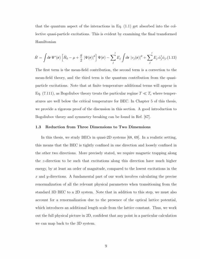
that the quantum aspect of the interactions in Eq. (1.1) get absorbed into the col-

lective quasi-particle excitations. This is evident by examining the final transformed

Hamiltonian

H =

∫dr Ψ∗(r)

[H0 − µ+

g

2|Ψ(r)|2

]Ψ(r)−

′∑j

Ej

∫dr |vj(r)|2 +

′∑j

Ej α†jαj.(1.13)

The first term is the mean-field contribution, the second term is a correction to the

mean-field theory, and the third term is the quantum contribution from the quasi-

particle excitations. Note that at finite temperature additional terms will appear in

Eq. (7.111), as Bogoliubov theory treats the particular regime T Tc where temper-

atures are well below the critical temperature for BEC. In Chapter 5 of this thesis,

we provide a rigorous proof of the discussion in this section. A good introduction to

Bogoliubov theory and symmetry breaking can be found in Ref. [67].

1.3 Reduction from Three Dimensions to Two Dimensions

In this thesis, we study BECs in quasi-2D systems [68, 69]. In a realistic setting,

this means that the BEC is tightly confined in one direction and loosely confined in

the other two directions. More precisely stated, we require magnetic trapping along

the z-direction to be such that excitations along this direction have much higher

energy, by at least an order of magnitude, compared to the lowest excitations in the

x and y-directions. A fundamental part of our work involves calculating the precise

renormalization of all the relevant physical parameters when transitioning from the

standard 3D BEC to a 2D system. Note that in addition to this step, we must also

account for a renormalization due to the presence of the optical lattice potential,

which introduces an additional length scale from the lattice constant. Thus, we work

out the full physical picture in 2D, confident that any point in a particular calculation

we can map back to the 3D system.

9

Strict confinement in the z-direction demands a clear separation between the

characteristic length scales associated with the interaction g, the average particle

density n, and the width of the BEC in the z-direction Lz. Note that throughout

this thesis we consider only the case where g > 0. The separation of length scales

is expressed in the inequality as Lz . ξ, where the transverse oscillator length

is determined by the oscillator frequency through Lz ≡ (~/Mωz)1/2, and the mass

M of the individual particles. The healing length in the BEC sets the upper bound

and is defined as ξ ≡ (8πnas)−1/2. Note that two length scales appear here: one is

the scattering length as and the other is the healing length ξ, which incorporates the

particle density n ≡ N/V , where N is the number of particles in the system and V

is the corresponding volume. A second condition is that the size of the condensate

along the large directions, defined by a radius R, is much larger than the transverse

direction Lz, R Lz, which for low temperatures and low energy stationary states

and dynamics, forces any accessible momentum states to lie only along the planar

direction of the BEC. Based on this discussion, we can separate the full 3D condensate

wavefunction into longitudinal and transverse parts, f(x, y) and h(z), respectively,

so that Ψ(r, t) = (ALz)−1/2 f(x, y)h(z)e−iµt/~, where A is the area πR2 and µ is the

chemical potential of the system. The reduction is completed by integrating over

the transverse direction z then redefining parameters to recover the 2D NLSE. In

Chapters 6 and 7, we explain how the interaction g is modified to obtain g2D along

with a full detailed analysis of our dimensional reduction procedure with complete

definitions of physical parameters.

1.4 Bose-Einstein Condensates in Two-Dimensional Optical Lattices

Bose-Einstein condensation was initially observed in dilute atomic gases of sodium,

lithium, and rubidium.4 Other elements which have been now Bose-condensed include

4We point out that the lithium observation was only confirmed two years after rubidium andsodium.

10

hydrogen, chromium, ytterbium, the alkali metals potassium and cesium, in addition

to the alkaline earth metals calcium and strontium, as well as dysprosium. The

BEC is typically observed at particle densities of 1012 cm−3 to 1014 cm−3 and as high

as 1015 cm−3 and at temperatures less than a microKelvin and as low as tens of

picoKelvin [70]. The cooling process occurs along a two step path: laser cooling

followed by evaporative cooling. The latter step allows higher energy atoms to leave

the system while further cooling the remaining atoms. Laser cooling is based on

the use of the Doppler effect for atoms interacting with a laser beam. To see this,

we consider two oppositely directed beams of the same frequency just below the

frequency of an atomic transition. An atom stationary with respect to both beams

will absorb an equal number of photons, of the same energy, from either direction.

Thus no net momentum change of the atom is observed. The key point here is that

the atomic absorption rate depends on the frequency of the absorbed light, so that we

can capitalize on the Doppler shift that occurs for motion towards or away from the

direction of a beam. The result is that an atom with a net velocity in one direction

will experience a frictional force opposite the direction of motion.

Two pervasive features which underlie our work are the concepts of condensation

and superfluidity. The Bose-Einstein condensate is synonymous with the breaking

of global U(1) symmetry [30, 31], resulting in long-range phase coherence, whereas

superfluidity derives from the BEC state but has more notions associated with it,

such as the Hess-Fairbanks effect [71]. Generally, the condensate phase refers to a

macroscopic number of particles residing in one single-particle state, whereas super-

fluidity refers to the response of particles to a velocity boost. We can understand the

meaning of U(1) symmetry breaking by returning to the Hamiltonian in Eq. (1.1). It

is symmetric under a global phase transformation, i.e., the transformation ψ → eiαψ

leaves the Hamiltonian unchanged, where α is a real constant. This symmetry is

described by the unitary group of degree one, or U(1). It is in some ways implied in

11

Eq. (1.1) that since we are working with the full many-body theory, the principle of

phase-density uncertainty is at work, and that in general the Hilbert space connected

to the field operator ψ is associated with a completely random phase. As we have

seen, the mean-field step which exchanges the condensate operator for a complex

wavefunction implies a completely well defined phase: the phase has acquired a non-

zero expectation value. This type of formal symmetry breaking is physically realized

in the case of a BEC, where the ground state of the system does not share the same

global U(1) symmetry of the underlying Hamiltonian.

These concepts become more tenuous when the constituent bosons are confined in

an optical lattice, since here macroscopic atomic coherence can be disrupted by the

periodic potential of the lattice. Nevertheless, one finds that BECs do indeed occur

in such systems as long as the lattice is shallow enough to avoid the Mott insulating

phase. In the lattice setting, particle interactions U and hopping th give rise to two

distinct phases associated with the strong and weak interaction limits U/th 1 and

U/th 1. When interactions are strong, particles tend not to occupy the same sites,

and we find that particle number is well defined at each site, with large uncertainty

in the phase. This defines a Mott insulator: shifting particles around is energetically

costly. For weak interactions, hopping is dominant so that the total energy of the

system is lowered when particles move freely through the lattice. In this case, on-site

particle number is uncertain, while the phase is well defined. This state defines a

superfluid with velocity defined as the gradient of the phase v ≡ (~/M)∇Φ, which

we discuss later in Section 1.4. Of critical importance to BEC stability is the strict

2D confinement which destroys long-range order as expounded in the Mermin-Wagner

theorem [72]. For a thorough treatment of the physics of cold atoms see Ref. [7] and

the review article [4]. For a good review on the theory of cold bosons in optical

lattices see Ref. [64], and [73, 74] for a treatments on 2D systems.

12

A quantum fluid may be described in terms of its normal versus superfluid frac-

tions fn and fs, the former pertaining to the viscous part and the latter referring

to that part of the fluid which flows unimpeded [75]. In particular, one precise way

to define the superfluid state is in terms of changes in the matter wave interference,

i.e., decoherence, quantified by the energetic cost of adding twists to the macroscopic

phase Φ of the BEC, where the macroscopically occupied wavefunction Ψ may be

expressed in terms of the density and phase Ψ(r) =√ρ(r) eiΦ(r) [76]. The velocity

field which describes superfluid flow is the usual phase gradient v ≡ (~/M)∇Φ.

The BEC ground state energy E0 is invariant under global changes in Φ but

not local, spatially dependent ones. The energetic cost δEΦ of adding small local

variations in Φ is interpreted as the additional kinetic energy due to the superfluid

flow. In the 1D linear approximation this leads to an expression for the superfluid

fraction fs = 4π2(EΦ−E0)/(NER∆Φ2), where N is the total number of particles, ∆Φ

is the phase variation over the lattice spacing a, and ER = ~2/(2Ma2) is the lattice

recoil energy, i.e., the kinetic energy characterized by the periodicity of the lattice [76].

In all of the problems we present in this thesis, we work in the long-wavelength limit

so that Φ is the phase of the complex Bloch factor and plays a central role in vortices

as the quantized winding around the core.

Closely related to the use of on-site localized atomic states is the notion of the

tight-binding approximation. Physically, this refers to the optical regime in which a

particle’s potential energy inside a single well is much larger than the characteristic

kinetic energy imparted to it by the lattice. This can be stated precisely as V0/ER

1, in terms of the lattice depth V0 and the recoil energy ER, where M is the mass

of the constituent bosons and k is the wavenumber of the laser light making up the

lattice. In our work we consider 1 V0/ER . 20: the lower bound is to satisfy the

tight-binding limit, while the upper bound comes from satisfying the various physical

constraints in our problem, including avoiding a Mott-insulating transition. The tight-

13

binding limit allows for a many-body description in terms of the nearest-neighbor

hopping picture where bosons reside mainly at individual lattice sites and tunneling

to adjacent sites is accounted for by including the strength of overlap between adjacent

Wannier peaks [62] encapsulated in the hopping energy th. Typically, the hopping

parameter th is computed using the semiclassical approximation, which provides an

accurate treatment such that th ≡ 1.861 (V0/ER)3/4ER exp(−1.582

√V0/ER

)[77].

The Bose-Hubbard model (BHM) is consistent with this picture, which we obtain

as an intermediate stage of our derivation of the nonlinear Dirac equation, and rely on

extensively well as the foundation of many of our other calculations. The derivation

of the BHM proceeds from the full many-body Hamiltonian for an interacting Bose

gas in a periodic external potential, followed by the assumption of tight-binding,

which allows for a Wannier basis expansion of spatially dependent terms. Finally, we

integrate over the spatial coordinates which leads to a discrete lattice Hamiltonian.

We present this derivation in detail in Chapter 2.2.1. Explicitly, the BHM is embodied

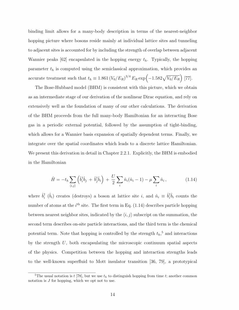
in the Hamiltonian

H = −th∑〈i,j〉

(b†i bj + b†j bi

)+U

2

∑i

ni(ni − 1)− µ∑i

ni , (1.14)

where b†i (bi) creates (destroys) a boson at lattice site i, and ni ≡ b†i bi counts the

number of atoms at the ith site. The first term in Eq. (1.14) describes particle hopping

between nearest neighbor sites, indicated by the 〈i, j〉 subscript on the summation, the

second term describes on-site particle interactions, and the third term is the chemical

potential term. Note that hopping is controlled by the strength th,5 and interactions

by the strength U , both encapsulating the microscopic continuum spatial aspects

of the physics. Competition between the hopping and interaction strengths leads

to the well-known superfluid to Mott insulator transition [36, 79], a prototypical

5The usual notation is t [78], but we use th to distinguish hopping from time t; another commonnotation is J for hopping, which we opt not to use.

14

example of a quantum phase transition (QPT) [80] observed in experiments [36].

Note that Eq. (1.14) is valid for arbitrary spatial dimensions. In particular, for the

2D honeycomb lattice, the BHM is expressed by the Dirac-Bose-Hubbard Hamiltonian

which we derive in Chapter 2, specifically in Eq. (2.10).

One unique feature of two-dimensional (2D) systems at finite temperatures is the

absence of condensation in the formal sense, i.e., a configuration with infinite phase

coherence. At nonzero temperature, long-wavelength thermal fluctuations destroy

the long-range order in a sample. This occurs in the interacting as well as non-

interacting case, and one must instead be content with a quasi-condensate order

characterized by phase coherence on finite length scales. In this case, the one-body

correlation function decays algebraically as opposed to exponential decay for the

ordinary uncondensed state. Nevertheless, the vortex and soliton structures which

we deal with have characteristic healing lengths which are small compared to the size

of the regions of coherence, and hence this limitation does not impose any noticeable

restrictions on our results.

The transition from ordinary to superfluid phase in 2D was originally predicted by

Berezinskii [81] and by Kosterlitz and Thouless (BKT) [82], and has been confirmed

for several macroscopic quantum systems [74]. A wide variety of 2D phenomena ex-

hibit this property including superfluid liquid helium films [83], superconductivity in

arrays of Josephson junctions [84], and collisions in 2D atomic hydrogen [11]. The

microscopic mechanism underlying the BKT transition is that of bound, oppositely

rotating pairs of vortices below a critical temperature Tc, contrasted with a prolifera-

tion of unbound individual vortices above Tc which destroy the long-range order. The

precise mechanism of the transition hinges on the abrupt phase dislocations which

occur at the core of a vortex contrary to the slowly varying phase interference fringes

coming from ordinary fluctuations in Φ.

15

Recently, it was shown that the BKT phase transition is a generic feature of a

large class of (2 + 1)-dimensional models which bridge non-relativistic and relativistic

many-body physics [85]. This new type of phase transition was obtained via holo-

graphic duality, thus the term holographic BKT has been coined. The honeycomb

optical lattice provides an ideal setting for studying the binding and unbinding of

exotic relativistic vortices not found in ordinary 2D BECs, and the associated BKT

transition at finite or zero temperature. Although we do not treat the full dynamics

of vortices in this thesis, our investigations into vortex solutions and their stability

properties provide the framework for further research into such phenomena as BKT

type transitions for relativistic systems. The underlying lattice allows for a large

variety of distinct vortices, and these are expected to play a central role in the corre-

sponding superfluid phase transition. To study BKT in our system requires a specific

relationship for our length scales. We would require that the BEC sample size R (ra-

dius), 2D healing length ξ, and lattice constant a satisfy the inequality a ξ R.

The first inequality pertains to the long wavelength approximation on the lattice,

while the second ensures that vortices are microscopic in relation to the sample size.

Incidentally, we adhere to this condition throughout our work.

1.5 Cold Atom Interactions in Optical Lattices and Magnetic Traps

In our work we consider samples of cold atoms confined in magnetic traps. Mag-

netic trapping of neutral atoms occurs through the Zeeman effect, which comes from

the interaction between electronic and nuclear spin magnetic moments and an ex-

ternal applied magnetic field. For low-strength magnetic fields, Zeeman energies are

small compared with hyperfine splitting, in which case the energy may be written as

E(F,mF ) = E(F ) +mFgFµBB , (1.15)

16

expressed to first order in the magnetic field B, where gF is the Lande g factor, E(F )

is the energy in the absence of an external magnetic field, F is the total spin, and

mF is the z-component of the total spin. The states which interest us are the ones

for which F = I − 1/2 with mF = −(I − 1/2), since they have negative magnetic

moments and are therefore amenable to magnetic trapping. A negative magnetic

moment means that atoms in such states will be forced towards a local minimum

when placed in an inhomogeneous magnetic field. Thus, the magnetic configuration

of interest is one with a local minimum, either a zero or a non-zero value of |B|.

The quadrupole trap is an example of the former and the Ioffe-Pritchard trap is an

example of the latter. Detailed explanations of the various types of traps may be

found in Ref. [7].

In the presence of a spatially varying electric field, neutral atoms experience a force

due to the polarization of their electronic charge distribution. For an inhomogeneous

time-varying electric field, the gradient of the shift in atomic energy gives rise to the

dipole force

Fdipole = −∇V (r) =1

2α′(ω)∇〈E(r, t)2〉t , (1.16)

where the bracketed quantity is the time-average of the applied electric field and

α′(ω) is the frequency dependent atomic polarizability. This is referred to as the AC

Stark shift. The direction of the polarizability is aligned with the electric field at

low frequencies (red-detuned) and anti-aligned for frequencies above critical atomic

transitions (blue-detuned). Thus, just below or above a resonance, the atom is forced

towards high-field regions and low-field regions, respectively. This leads directly to

the notion of using interfering laser beams to create standing waves with alternating

regions of peaks and zeros in the electric field. The resulting periodic optical lattice

potential can be used to trap atoms either at the regions of strong or weak electric

field for the red-detuning versus blue-detuning case. In Figure 1.1(a), we illustrate

17

!"#

!"#$%&'#()

#*+,'-.!.-++,'%!

!!!!!!.-/%0/

!!"#$%&'()!

)&'*('+%+',!

y

x

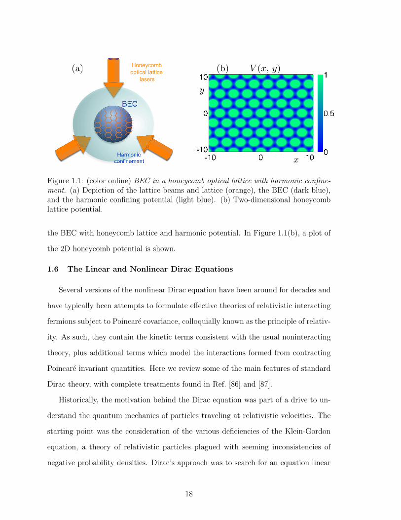
(a) (b) V (x, y)

Figure 1.1: (color online) BEC in a honeycomb optical lattice with harmonic confine-ment. (a) Depiction of the lattice beams and lattice (orange), the BEC (dark blue),and the harmonic confining potential (light blue). (b) Two-dimensional honeycomblattice potential.

the BEC with honeycomb lattice and harmonic potential. In Figure 1.1(b), a plot of

the 2D honeycomb potential is shown.

1.6 The Linear and Nonlinear Dirac Equations

Several versions of the nonlinear Dirac equation have been around for decades and

have typically been attempts to formulate effective theories of relativistic interacting

fermions subject to Poincare covariance, colloquially known as the principle of relativ-

ity. As such, they contain the kinetic terms consistent with the usual noninteracting

theory, plus additional terms which model the interactions formed from contracting

Poincare invariant quantities. Here we review some of the main features of standard

Dirac theory, with complete treatments found in Ref. [86] and [87].

Historically, the motivation behind the Dirac equation was part of a drive to un-

derstand the quantum mechanics of particles traveling at relativistic velocities. The

starting point was the consideration of the various deficiencies of the Klein-Gordon

equation, a theory of relativistic particles plagued with seeming inconsistencies of

negative probability densities. Dirac’s approach was to search for an equation linear

18

in the time derivative as well as the spatial ones, and he thus came upon the gamma

matrices. His motivation was based partly on a deep intuition about the way physics

equations should look. This appeal to aesthetics was the source of his creative inspira-

tion so it is not surprising that the Dirac equation should exhibit a rich mathematical

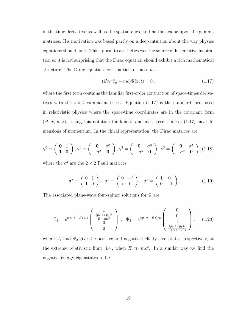
structure. The Dirac equation for a particle of mass m is

(i~γµ∂µ −mc)Ψ(r, t) = 0 , (1.17)

where the first term contains the familiar first-order contraction of space-times deriva-

tives with the 4 × 4 gamma matrices. Equation (1.17) is the standard form used

in relativistic physics where the space-time coordinates are in the covariant form

(ct, x, y, z). Using this notation the kinetic and mass terms in Eq. (1.17) have di-

mensions of momentum. In the chiral representation, the Dirac matrices are

γ0 ≡(

0 11 0

), γ1 ≡

(0 σx

−σx 0

), γ2 =

(0 σy

−σy 0

), γ3 =

(0 σz

−σz 0

), (1.18)

where the σi are the 2× 2 Pauli matrices

σx ≡(

0 11 0

), σy ≡

(0 −ii 0

), σz =

(1 00 −1

). (1.19)

The associated plane-wave four-spinor solutions for Ψ are

Ψ1 = ei(p · r−E t)/~

1

(px + i py)c

E+mc2

00

, Ψ2 = ei(p · r−E t)/~

001

(px + i py)c

−(E+mc2)

, (1.20)

where Ψ1 and Ψ2 give the positive and negative helicity eigenstates, respectively, at

the extreme relativistic limit, i.e., when E mc2. In a similar way we find the

negative energy eigenstates to be

19

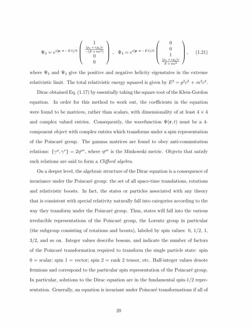
Ψ3 = ei(p · r−E t)/~

1

(px + i py)c

−(E+mc2)

00

, Ψ4 = ei(p · r−E t)/~

001

(px + i py)c

E+mc2

, (1.21)

where Ψ3 and Ψ4 give the positive and negative helicity eigenstates in the extreme

relativistic limit. The total relativistic energy squared is given by E2 = p2c2 + m2c4.

Dirac obtained Eq. (1.17) by essentially taking the square root of the Klein-Gordon

equation. In order for this method to work out, the coefficients in the equation

were found to be matrices, rather than scalars, with dimensionality of at least 4× 4

and complex valued entries. Consequently, the wavefunction Ψ(r, t) must be a 4-

component object with complex entries which transforms under a spin representation

of the Poincare group. The gamma matrices are found to obey anti-commutation

relations: γµ, γν = 2ηµν , where ηµν is the Minkowski metric. Objects that satisfy

such relations are said to form a Clifford algebra.

On a deeper level, the algebraic structure of the Dirac equation is a consequence of

invariance under the Poincare group: the set of all space-time translations, rotations

and relativistic boosts. In fact, the states or particles associated with any theory

that is consistent with special relativity naturally fall into categories according to the

way they transform under the Poincare group. Thus, states will fall into the various

irreducible representations of the Poincare group, the Lorentz group in particular

(the subgroup consisting of rotations and boosts), labeled by spin values: 0, 1/2, 1,

3/2, and so on. Integer values describe bosons, and indicate the number of factors

of the Poincare transformation required to transform the single particle state: spin

0 = scalar; spin 1 = vector; spin 2 = rank 2 tensor, etc. Half-integer values denote

fermions and correspond to the particular spin representation of the Poincare group.

In particular, solutions to the Dirac equation are in the fundamental spin-1/2 repre-

sentation. Generally, an equation is invariant under Poincare transformations if all of

20

its terms transform with the same numbers of factors of the Poincare group or factors

of its spinor representation. This idea is illustrated in further detail in Chapter 3.3,

where we work out the Poincare structure of our nonlinear Dirac equation.

In high energy physics, the mass term in the Dirac equation has an intuitive

meaning as the minimum energy needed to produce real (non-virtual) particles during

collisions. The analogous concept for periodic condensed matter systems is the mass

gap, i.e., the finite gap which separates two energy bands. In a crystal, the gap appears

at the edge of the reciprocal lattice when the periodic particle density undergoes a

rigid spatial translation by half the period of the lattice, while keeping the crystal

momentum fixed. The energy shift is just the energy difference that comes from

shifting the position of the density peaks from the minima to the maxima of the

background lattice potential. Graphene represents a semi-metal, as there is no gap

due to the bands crossing at the Dirac point; the NLDE also has no gap. The crossing

is due to degeneracy in A and B sublattices. A staggered lattice or other method that

breaks the degeneracy of A and B sublattices can be used to deform the Dirac point

and open up a band gap. In Chapter 8.4, we introduce the different mass gaps for the

NLDE and obtain gap solitons. Although mass gaps are easy to implement in optical

lattices, for simplicity, we focus here on the Dirac equation with the mass term set

to zero, m = 0 in Eq. (1.17). This describes the behavior of massive fermions in the

extreme relativistic limit, as well as the flow of charge carriers in graphene and cold

bosonic and fermionic atoms in honeycomb-optical-lattice condensed matter systems.

There are two key representations of the gamma matrices, each one emphasizing

one of two extreme perspectives. In the energy representation, the upper and lower

2-spinors which make up ψ are positive and negative-energy eigenstates, respectively:

changing from positive to negative energy does not mix the 2-spinors. On the other

hand, in the chiral representation, the upper and lower 2-spinors are positive and

negative-helicity eigenstates: changing from positive to negative helicity does not

21

mix these 2-spinors. This is explained in mathematical detail in the first part of

Chapter 3.3. Helicity measures the projection of spin in the direction of momentum

and the helicity operator is exactly the nonzero 2 × 2 subspace of the kinetic part

of the massless Dirac Hamiltonian – off diagonal subspaces in the energy represen-

tation and diagonal subspaces in the chiral representation. Interestingly, there is an

elegant formulation of the massless Dirac equation in 2D as the simplest example of

a supersymmetric theory, namely N = 2 supersymmetry [88]. The two generators

or supercharges, indicated by the N -value, are the nonzero 2 × 2 subspaces of the

Hamiltonian.

The earliest versions of the NLDE were motivated by the need to reduce the com-

plexity of subatomic phenomena down to workable models which one could solve using

well know mathematical tools. As the use of complicated field theoretic methods be-

came the mainstay for describing relativistic interactions, various other methods were

developed in parallel. Phenomenological models were developed in which complicated

quantum effects could be encapsulated into nonlinear terms which were incorporated

into semiclassical field equations. Such effective models offered the advantage of be-

ing intuitive as well as easier to work with, while still retaining some of the essential

physics of the full theory. Among the most notable nonlinear modifications of the

Dirac equation were the nonlinear spinor models proposed by D. D. Ivanenko [89],

W. Heisenberg [90, 91], R. Finkelstein [92, 93], and F. Gursey [94]. These were de-

signed to account for the self-energy of the electron in the ambient electromagnetic

background.

Remarkably, the techniques developed for solving a wide variety of NLDEs have

also been used to construct multi-parameter families of exact solutions for many

other nonlinear systems [95]. Systems of partial differential equations which have

been solved using nonlinear Dirac techniques include Dirac-d’Alembert, Maxwell-

Dirac, d’Alembert-eikonal, SU(2) Yang-Mills, and Levy-Leblond among others. A

22

good review of these methods can be found in Ref. [95]. The NLDE has been applied

to many contemporary problems as well. In optics, for example, the NLDE has

been used as an effective description of Maxwell’s equations in the slowly varying

envelope approximation for photonic crystals [96]. From a mathematical standpoint,

classifications of stationary solutions of NLDEs are generally restricted to (3 + 1)-

dimensions, and to classes of nonlinear terms of the form F (ψ)ψ, where F ∈ C2(C4,R),

ψ : R3 → C4, and commonly F (ψ) ≡ λ(|ψψ|α+b|ψγ5ψ|β), with 1 < α, β < 3/2 ; λ, b >

0 [95, 97, 98]. Note that in this form F (ψ)ψ is Poincare invariant, whereas for the

NLDE which we study in this thesis the nonlinearity does not factor in the same way.

An exception to this is the case of NLDE in optics which breaks Poincare covariance.

It is important to point out that our NLDE arises naturally out of BECs in honeycomb

optical lattices, whereas other NLDEs were purely theoretical constructs.

Formal mathematical treatments of the NLDE focus on defining the bounds, sta-

bility, and scope of well-posedness from a purely theoretical standpoint [98–102], while

other treatments focus more on explicit solutions by capitalizing on the symmetries

of the NLDE [95, 103]. A rigorous exposition of the various nonlinearities which pre-

serve Poincare invariance can be found in Ref. [97], where the NLDEs are classified

by the degree of the nonlinearity and the number of derivatives it contains. For a

good introduction to the subject of NLDEs see Ref. [104].

In the literature, one generically encounters the NLDE in a condensed form ex-

pressed as

i~ ∂tΨ − DmΨ + G(Ψ) = 0 , (1.22)

where the notation G(Ψ) indicates a functional of Ψ, and contains the interaction

terms. The form of Eq. (1.22) differs from that of Eq. (1.17) in that the space and time

derivatives have been separated as a first step towards obtaining explicit solutions.

Note that in Eq. (1.22) the space-time coordinates are (t, x, y, z). In addition, we

23

have defined Dm ≡ −i~c γj∂j+mc2, which contains the spatial derivatives contracted

with gamma matrices (j = 1, 2, 3) and includes the mass gap structure indicated by

the subscript m. The mass term is just the subtraction of a constant from the

derivative terms. The nonlinear terms are contained in the functional G ∈ C1(C4,C).

The usual analysis is to consider stationary solutions, i.e., a separation of variables

between time and space, for which solutions to Eq. (1.22) are of the form: Ψ(r, t) =

e−iωtψ(r), where ψ is also a four-spinor and solves the time-independent NLDE,

−~ω ψ − Dm ψ + G(ψ) = 0 , (1.23)

where we retain the same notation as in Eq. (1.22). The functionalG(ψ) is parametrized

by the interaction strength U . In the literature, the nonlinear terms in G(ψ) are con-

strained to be a Poincare invariant (usually scalar or vector quantities) to coincide

with most particle physics models. It is important to state that Poincare invariance

places a strong restriction on the form of G(ψ) and these types of NLDEs only admit

localized solutions for eigenvalues inside the gap, 0 < ~ω < mc2, and nonexistence

of localized solutions for |ω| > 1 [105, 106]. This is because invariance under a gen-

eral Poincare transformation forces the radial amplitudes within each of the upper

and lower two-spinors of ψ to be equal, which greatly limits the variety of possible

combinations in the derivative terms. However, for the NLDE that we obtain, this

severe restriction is lifted and the form of the equations allow for localized eigenval-

ues within the continuous spectrum, i.e., for ~|ω| ≥ mc2, as well as inside the gap,

−mc2 < ~ω < mc2.

One also encounters the nonlinear Dirac operator as Dm,U = Dm−G(ψ) such that

Eq. (1.22) is

Dm,U ψ − ω ψ = 0 . (1.24)

24

This is indeed possible even though the range of Dm,U depends on elements of the

domain [107, 108]. The nonlinear Dirac equation can be derived from a variational

principle with the corresponding action being given by

Iω(ψ) =

∫R2

d2x

[1

2

(ψ†, Dm ψ

)− 1

4ω ψ†ψ − G(ψ)

], (1.25)

where G is the functional integral of G, i.e. G(ψ) = δδψG, the contraction

(ψ†, Dm ψ

)is the L2 contraction defined by

(ψ, ψ′)L2 =

∫R2

d2x ψ ψ′ .

(1.26)

Eq. (1.23) is the Euler-Lagrange equation associated with Eq. (1.25). It is important

to note that since the spectrum of Dm is not positive-definite, solutions of Eq. (1.23)

do not minimize Eq. (1.25), that is, the spectrum of the NLDE is not bounded below:

there is no ground state in the strict sense.

1.7 Nonlinear Dirac Equations in Condensed Matter and Cold AtomicGases

As we show in this thesis, the NLDE can be realized by forming a BEC in the

lowest Bloch band of a honeycomb optical lattice [109]. The lattice is constructed

using three sets of interfering laser beams in a plane while tightly trapping atoms

in the vertical direction to obtain a quasi-2D system. Atoms are condensed into the

lowest energy state of the lattice and then transferred to the Dirac points by Bragg

scattering combined with a series of switching steps to turn off and on interactions

of the atomic hyperfine states with the lattice laser beams. This method allows for

a stable transfer of atoms to the Dirac points. An alternative approach involves an

adiabatic acceleration of the lattice to get the BEC to the Dirac points, but the first

approach eliminates potential dynamical instabilities which may arise from a moving

25

lattice. It should be noted that the Dirac point is maintained in the presence of the

shallow harmonic trapping potential [110]. As described in Sec. 1.5, the laser interfer-

ence pattern interacts with the atoms of the condensate via the AC Stark effect, thus

creating a two-dimensional periodic potential; as described in Chapter 7, the third

spatial dimension frozen out by a tightly confining potential in that direction [74].

From a theoretical standpoint, as shown in Chapt. 2, the NLDE is derived by

starting from the second quantized Hamiltonian for a weakly interacting bosonic gas

in two spatial dimensions and then imposing the tight-binding limit which involves

expressing the bosonic field operators in terms of Wannier functions, a natural ba-

sis for periodic systems. Upon integrating over the two spatial degrees of freedom

keeping only nearest neighbor tunneling, the Hamiltonian reduces to a discrete lattice

form: the Bose-Hubbard model for the honeycomb lattice. Translating to the edge of

the Brillouin zone and taking the expectation value with respect to on-site coherent

states (which projects from a second quantized theory down to a mean-field one), and

finally, taking the continuum limit produces the NLDE. By taking a superposition of

theories for two opposite Dirac points, we obtain the full NLDE [52]. The nonlinear

interactions are proportional to the density of the BEC and each term contains fac-

tors of the same spinor component – nonlinear terms do not couple different spinor

components. Similar equations have been vigorously studied in the literature, in the

context of particle and nuclear theory [111–114] as well as in nonlinear dynamics and

applied mathematics [95, 115–119], but our particular version of the NLDE had not

been studied before in connection with BECs or otherwise, and there was no experi-

mental realization of any NLDE in any field before our work in 2009 [52]. In Chapts. 2

and 8, we obtain massless and massive versions of the NLDE as well as zigzag and

armchair forms of the 1D NLDE, all with the same form for the nonlinear terms.

.

26

1.8 Connections to Optics and Applied Mathematics

A major area of research into NLDE physics outside of cold atoms is the study of

diabolical points in optics. This concept originated in a combination of experiments

where a randomly polarized ray of light traveling through a biaxial crystal exhibits

cone shaped diffraction due to a singularity in k space from the polarization of the

beam. More recently, inspired by conical Dirac points in honeycomb lattices, there has

been much interest in obtaining diabolical point structures for optical waves traveling

in honeycomb photonic crystals [120]. These have been studied numerically and have

been experimentally detected. Other topics based on relativistic physics of Dirac

points have also been investigated in honeycomb photonic crystals, such as symmetry

breaking in the Dirac cone [121] and P-T symmetry, as well as problems in nonlinear

physics such as gap solitons [120], which play an important role in our work. Another

field where the honeycomb lattice structure is used to get Dirac dispersion is in an

acoustic setting [122].

Partly because of the nonlinearity associated with conical diffraction, research

in applied mathematics has also been stimulated. From the mathematical point

of view, conical diffraction arises in the nonlinear Schrodinger equation when the

external potential has a honeycomb shape. Both analytical derivations and numerical

simulations for the wave envelope of Bloch modes in a honeycomb lattice potential

have confirmed conical diffraction. Such approaches work directly from the NLSE,

and show that the dynamics of the wave envelope is governed by the NLDE [123].

Significantly, the results of Ablowitz, Nixon, and Zhu show that when tight-binding

in the lowest band is assumed, conical diffraction is maintained in the presence of

nonlinearity [20, 123].

Investigations into nonlinear Dirac physics using numerical methods based on the

NLSE and accounting for higher band structure beyond the lowest band, have also

been implemented [32]. These calculations reveal that nonlinearity alters the structure

27

of the Dirac cone by changing the topology at the Dirac points for arbitrarily small

interaction, suggesting a breakdown of the superfluid phase. These results provide key

insights into Dirac point structure when the tight-binding, lowest band approximation

does not hold. However, as long as lattice parameters and interactions are chosen

such that the lowest-band approximation is warranted, it is our contention that the

integrity of the Dirac cone will be preserved. A numerical investigation of NLDE

vs. full NLSE with honeycomb lattice dynamics to support our scaling arguments is

reserved for future work. In addition, another intriguing method worth mentioning

for simulating the 1D NLDE is by using a single trapped ion which can be shown to

mimic a free relativistic quantum particle [124].

1.9 Approximations and Constraints Involved in the Nonlinear DiracEquation

Realization of the NLDE physics requires that several physical constraints are sat-

isfied. For example, we have already touched on the problem of dimensional reduction,

which, as we have seen, determines an upper bound on the order of magnitude of the

s-wave scattering length, and a lower bound on the oblateness of the condensate, for a

given value of the particle density. The density n and its dimensionally reduced form

n2D ≡ Lzn, are central, and appear in the definitions of many important quantities

and their renormalized counterparts. The constraints which need to be satisfied can

be broken down into categories involving the following sets of physical quantities: the

energies and lengths for the 3D to 2D reduction; the characteristic speeds of the 2D

lattice theory versus the unconfined 3D theory; the relative strengths of interactions

to hopping between lattice sites must be correctly tuned for a stable superfluid state;

quasi-particle, Dirac point, and lattice recoil momenta are interrelated to ensure that

the Dirac cone and long-wavelength limits are valid and the relative strength of the

potential depth to the recoil energy of the lattice to ensure that the lowest-band and

tight-binding approximations hold.

28

Several length and energy parameters are fundamental to the NLDE, with other

composite quantities formed from these. The fundamental lengths are the transverse

width and longitudinal radius of the BEC, Lz and R⊥, the honeycomb lattice con-

stant a, the s-wave scattering length as, and the average inter-particle distance n−1/3.

The fundamental energy scales are determined by the lattice depth V0, the thermal

Boltzmann energy kBT , and the chemical potential of the system µ. All of these pa-

rameters are related in a complicated way through the constraints, with the region of

validity for the NLDE lying within the boundaries defined by these constraints. For

example, the following offers one consistent set of length parameter values for a BEC

made up of 87Rb atoms in a honeycomb lattice, to support the NLDE: Lz = 3.0µm,

R⊥ = 55.0µm, a = 0.55µm, as = 5.77 nm, and n−1/3 = (1×1016 m−3)−1/3 = 4.64µm.

Values of the energy parameters consistent with these lengths are V0 = 2.60µK,

kBT = 8.0 nK, and µ = 2.36 nK. A complete description of NLDE parameters and

constraints can be found in Chapters 6 and 7 of this thesis, specifically in Tables 6.1

and 7.1.

1.10 Solution Methods for the Nonlinear Dirac Equation

The stationary localized solutions of the NLDE we obtain fall into either of two

categories: two-dimensional vortices and one-dimensional solitons. Vortices are char-

acterized by having a core defined by a phase jump, or singularity, with quantized

rotational angular momentum circulating around the core. Our soliton solutions solve

the 1D NLDE obtained by integrating out one of the planar spatial directions. Phys-

ically, this arises when the trap length in one direction is made small compared to the

other direction. To obtain these solutions in the chiral representation of the NLDE,

we start by splitting the full four-spinor NLDE into two equivalent sets of coupled

equations for each pair of two-spinors, and specialize to stationary wavefunctions to

arrive at:

29

µψA + i ~clD∗ψB − U |ψA|2 ψA = 0 (1.27)

µψB + i ~clD ψA − U |ψB|2 ψB = 0 , (1.28)

where µ is the chemical potential, cl is the effective speed of light, U is the interaction

strength, and D ≡ (∂x + i ∂y) is the Dirac differential operator.

We obtain soliton solutions to Eqs. (1.28) by freezing out one spatial dimension

as stated above. Retaining only the y-direction in Eqs. (1.28) results in equations

for propagation in the armchair geometry of nanoribbon, whereas retaining the x-

direction gives the zigzag geometry analogous to the two forms of graphene nanorib-

bon geometries. We then express the wavefunction in terms of envelope and internal

component functions: Ψ(x) = η(x) [cosϕ(x), sinϕ(x)]T , where we let x denote either

direction in Eq. (1.28). This step allows us to obtain a formal integral for η in terms

of ϕ, for which an exact solution is obtained when µ = 0. For more general soliton

solutions (µ 6= 0), we find solutions for which ϕ is approximately linear in x. We show

that such approximate solutions are valid as long as ϕ is a slowly varying function

in x. The second method that we use to obtain soliton solutions is to expand the

envelope η in a power series in the quantity cos4ϕ + sin4ϕ. We find this to be a

natural expansion argument given the way that it appears in the transformed version

of Eqs. (1.28). By solving consistently for the expansion coefficients, we are able to

obtain solutions which are more general than those obtained by the first method. An

important property of the series solution is that the terms connect to the solutions for

slowly varying ϕ above, when the parameters U and µ are appropriately tuned. When

a mass gap is turned on, a mapping of a subclass of NLDE solutions to the massive

Thirring model is possible. The massive Thirring model is was originally formulated

as a low energy effective theory of interacting fermions, integrable at both classical

and quantum mechanical levels [125, 126]. The advantage of this mapping is that

properties and solutions of the Thirring system are well understood and may then

30

be translated to the NLDE. We find that NLDE solutions obtained by this method

are qualitatively similar to the bright solitons obtained through the slowly varying ϕ

method.

We obtain seven different types of vortices by a variety of analytical methods.

To obtain vortex solutions, we first express Eqs. (1.28) in plane-polar coordinates,

then factor out the quantized angular dependence from the solution to arrive at two

coupled first order equations for the radial parts fA(r) and fB(r) of the component

wavefunctions ψA(r, θ) and ψB(r, θ). Our first method uses an asymptotic Bessel

expansion, which matches the asymptotic form of the vortex near the core and far

from the core, and gives us an approximate solution for large winding number, in

addition to deeper insight into the effect of the nonlinearity on solutions. A second

method is to write fA and fB as general algebraic expressions in the radial coordinate

r, up to arbitrary parameters. Substituting into the NLDE allows us to solve for the

extra parameters in a consistent manner. The algebraic method leads to a large class

of solutions for any winding number `. Specifically, when ` = 1, solutions exist for

the case µ = 0 and for µ > 0, in the form of a vortex with bright soliton at the core:

a ring-vortex with vanishing tail for the first case, and a vortex with asymptotically

constant (non-zero) tail for the second case. For ` > 1, we find algebraic closed forms

with chemical potential µ = 0, characterized by an asymptotically vanishing tail at

large r. These are general ring vortices where both spinor solutions vanish at the

core. For ` = 1, we also find skyrmions and half-quantum vortices by expressing

the wavefunction in terms of the envelope and internal spinor parts, η(r) and ϕ(r),

similar to the 1D case, then solving the resulting nonlinear system in η and ϕ.

Numerical solutions for both solitons and vortices are also obtained. In the case

of vortices, we first separate the quantized angular part from the radial part, then

solve the 1D radial equation by discretizing the derivatives using forward-backward

finite differencing and tuning the number of grid points until the desired precision of

31

convergence is obtained. We use numerical shooting by first expanding the solution

in a power series near the peak of the soliton, or the core of the vortex, then from

this we derive the behavior of the solution near that point. The vortex solution must

vanish at the core because of the angular momentum term, which adds an additional

condition on the wavefunction.

1.11 Overview of Thesis

This thesis is organized such that most chapters are separate articles published

(Chapters 2, 4), presently under review (Chapters 6, 8), or soon to be submitted

in a peer-reviewed journal (Chapters 7, 9). Some additional material is included in

Chapters 3 and 5 for overall clarity. The bibliography is placed at the end of the

thesis as many references are common to more than one chapter. The nature of the

work in this thesis is interdisciplinary and in general we adhere to the same notation

throughout consistent with condensed matter physics. The notation and definitions

for physical constants are summarized in Chapter 7.2.1 in particular in Table 7.1.

However, in certain places it is sometimes more convenient to use notation more in

line with high energy physics where covariance is explicit. This is done in order to

help bridge the gap between condensed matter and particle physics. In this overview,

we will address deviations from the standard notation of Table 7.1 for each chapter.

In Chapter 2, we derive the NLDE for BECs in honeycomb lattices and provide

a thorough symmetry analysis with comparison to the standard Dirac theory. This

section sets the foundation for the rest of the material in this thesis by providing a

rigorous derivation of the NLDE using well established tools of many-body theory

founded on coherent states for lattices. The section on symmetries clearly categorizes

our theory within the larger NLDE picture. The properties of the NLDE under

Poincare transformations pertains to the full 2D equations, in contrast to the 1D

problem which is treated later in the thesis. In this chapter the derivations use

explicit notation for physical parameters which include the effective speed of light

32

cl and Planck’s constant ~ with the usual (2 + 1)-dimensional coordinate notation

(t, x, y). In places where we want to emphasize the covariance of the NLDE, we use

the coordinate form (clt, x, , y). The derivation and resulting NLDE is unique and

appears here in the context of BECs for the first time.

In Chapter 3, we study additional fundamental topics in the NLDE. We summarize

the key points of the standard Dirac formalism, and provide a detailed analysis of

the structure of the NLDE. The Lagrangian formulation is presented and analyzed

with a view towards obtaining localized soliton and vortex solutions in addition to

a connecting to the nonlinear sigma model. We place the NLDE within established

mean-field theory by showing how it reduces to the NLSE with correction terms,

and study the soliton and vortex landscape of the corrected NLSE. These additional

correction terms result in a completely new type of NLSE. In addition, we address

a fundamental issue regarding spin-statistics. The spin-statistics theorem provides

the step which relates the geometric phase associated with Dirac points to the quasi-

particle operator statistics and clarifies how Dirac physics describing fermions can

arise out of a weakly interacting Bose gas. Our model offers a novel method for

realizing a transition from Bose to Fermi statisitics.

Chapter 4 provides an overview and first look at localized solutions of the NLDE

and the relativistic linear stability equations (RLSE), which determine the first or-

der effect of quantum fluctuations on arbitrary solutions of the NLDE. Experimental

signatures such as Cherenkov radiation and preliminary lifetime calculations are ob-

tained naturally from the RLSE. The interplay between quantum effects contained in

the Dirac dispersion and particle interactions reveal two low energy regimes defined

by, first, the lattice spacing, and second, the 2D renormalized healing length, the

length scale set by the strength of the 2D two-body interactions. Fluctuations much

larger than both the healing length and the lattice spacing behave as composite Dirac

particles. Such fluctuations are large enough that interactions blur the individual chi-

33

ral Dirac quasi-particles set up by the bipartite lattice. The chiral Dirac structure

is recovered for fluctuations with wavelengths comparable to the healing length but

still much larger than the lattice spacing. The RLSE are a completely new set of

equations derived for quasi-relativistic systems in BECs.

In Chapter 5, we provide the full detailed calculations of the RLSE eigenvalues and

the quasi-particle coherence factors for the case of a uniform condensate. We present

topics unique to this thesis which include symmetries of the RLSE, derivations of the

quasi-particle normalization conditions, classification of the different types of spinor

quasi-particle excitations, and approximate analytical solutions for general vortex

backgrounds.

In Chapter 6, we present the parameters and constraints key to observing Dirac

physics in BECs, along with the experimental procedures for setting up the optical

lattice, establishing the BEC at the Dirac points, and exciting the desired vortex

states. All of these topics are unique in that our experimental studies and particular

solutions in the context of honeycomb lattice BECs at Dirac points have not been

presented before. By accessing the internal atomic hyperfine degrees of freedom, we

show that our method allows one to populate Dirac points with a stable macroscopic

sample of cold bosonic atoms. We include a first look at topics such as vortex structure

and spectra. The notation in this chapter is based on Table 7.1 with the exception

of the general length scale r0 which is used to denote either the scale set by the

interaction ~cl/U , or that set by the chemical potential ~cl/µ.

Chapter 7 explores the complete vortex landscape for the full 2D NLDE. The

NLDE allows for seven distinct types of vortices distinguished by their phase winding

number and their asymptotic radial behavior far from the core. The macroscopic

phase encircling a vortex core may involve the internal spinor degrees of freedom,

as in the case of our skyrmions, or may only pertain to the overall phase, as in

many other NLDE solutions. Significantly, the 2D lattice allows for a half-quantum

34

vortex with half-integer phase winding. We present detailed analysis of analytical and

numerical vortex solutions, including stability analysis by solving the RLSE for vortex

backgrounds and calculating spectra for bound states in a weak confining potential.

The solutions, stability studies and spectra are new since our particular form of NLDE

is novel.

In Chapter 8, we solve the one-dimensional (1D) version of the NLDE and investi-

gate the types of gaps possible in this physical setup. For the case of zero gap, we ob-

tain solitons by a direct method, a soliton series expansion method, and by numerical

shooting. The first two methods provide consistency cross-checks for bright-solitons,

and the series method in particular gives us insight into possible integrability of the

1D NLDE. Numerical shooting gives us a dark soliton solution not accessed through

the first two methods. We calculate lifetimes by solving the 1D RLSE to obtain

the quasi-particle amplitudes and energies. The inclusion of a mass gap reveals two

mappings: one from the massive NLDE to the massive Thirring model and another

from the massless NLDE to the massive NLDE. From a practical point of view, these

mappings establish a dictionary translating from readily obtained soliton solutions in

one theory to new solutions in another. We encounter the topic of integrability here,

since the massive Thirring is well known to be integrable. Finally, the discrete spectra

which we obtain for bound solitons in a harmonic trap clearly delineate the energetic

signature for the gray solitons. The calculation of bound states leads directly into

the physics of Klein-tunneling, a feature of relativistic fermions not yet observed in

high-energy experiments.

In Chapter 9, we establish a quantum field theory at the Dirac points of the lattice

obtain the new result that bosons are described by a relativistic quantum field theory

for Dirac spinors. In addition, we derive the full many-body Hamiltonian for bosons

in the honeycomb lattice. We obtain the first-order momentum contribution which

gives the full quantum theory for a massless Dirac spinor. In addition, we compute

35

the second order correction term beyond the linear Dirac theory. This term describes

deviations from the linear approximation, and gives the quadratic contribution to

the dispersion in the associated mean-field theory. By using Hubbard-Stratonovich

decomposition, we derive the continuum quantum field theory at the Dirac points

and obtain the Lagrangian for interacting relativistic Dirac spinors.

Finally, in Chapter 10 we conclude by presenting several topics for future research

in the NLDE.

36

CHAPTER 2

THE NONLINEAR DIRAC EQUATION IN BOSE-EINSTEIN CONDENSATES:

FOUNDATION AND SYMMETRIES

Publication: L. H. Haddad and Lincoln D. Carr, Physica D: Nonlinear

Phenomena, 238, 1413-1421 (2011).

Abstract

We show that Bose-Einstein condensates in a honeycomb optical lattice are de-

scribed by a nonlinear Dirac equation in the long wavelength, mean field limit. Unlike

nonlinear Dirac equations posited by particle theorists, which are designed to preserve

the principle of relativity, i.e., Poincare covariance, the nonlinear Dirac equation for

Bose-Einstein condensates breaks this symmetry. We present a rigorous derivation of

the nonlinear Dirac equation from first principles. We provide a thorough discussion

of all symmetries broken and maintained.

37

2.1 Introduction

Recently the first truly two-dimensional (2D) solid state material, graphene, was

created in the laboratory [127, 128]. One of the most exciting aspects of this novel

material is that long wavelength excitations are described by a Dirac equation for

massless particles, with a “speed of light” equal to the Fermi velocity vF ' c/300 [48].

Thus one can study relativistic phenomena at very low velocities in an experiment far

more accessible than a particle accelerator. The lattice structure of graphene has also

led to insights into exotic features such as the integral and fractional quantum hall

effects [129]. The only real requirement to obtain this equation is the honeycomb

lattice structure of the graphene [16, 130–132]. One can therefore consider any solid

state system constructed on a honeycomb lattice, including artificial systems, in order

to study relativistic phenomena in novel materials accessible in tabletop experiments.

The most precise, cleanest, most controllable artificial solid state system is ultra-

cold atoms in optical lattices. Such systems have no impurities and no disorder unless

specifically added in by hand. They are very versatile: they can be constructed of

both bosons and fermions, of atoms and/or diatomic molecules, and can even have

a pseudospin structure. Their temperature, interactions, and symmetries can be

controlled externally. Moreover, 2D physics has recently been of great interest in

this context, in the form of the Berzinskii-Kosterlitz-Thouless crossover [74], and 2D

systems underpinned by lattices are immediately available in experiments. Instead of

considering ultra-cold fermions, which could be used to produce an near-exact analog

of graphene [133], we consider ultra-cold bosons. Other bosonic systems have been

studied in Refs. [70, 134–136], as well as systems composed of fractional numbers

of fermions of relevance to condensed matter as well as relativistic quantum field

theory [137, 138] . Systems of ultra-cold fermions have been used to study Bosonic

statistics and interactions lead to a new feature in the massless Dirac equation known

in graphene: a naturally occurring nonlinear term, giving rise to a nonlinear Dirac

38

equation. An important distinction should be made regarding preparation. For the

case of graphene it is the Fermi energy that brings the system to the Dirac point.

To bring the BEC to the Dirac point involves creating the condensate first then

adiabatically turning on the lasers in such a way as to create a moving lattice relative

to the condensate thus resulting in a condensate with nonzero lattice momentum [70].

The study of nonlinear phenomena in ultra-cold atoms, especially in Bose-Einstein

condensates (BECs) [4, 6], has been enormously fruitful. The recent text edited by

Kevrekidis, Frantzeskakis, and Carretero-Gonzalez provides an excellent summary of

this field [19]. The nonlinear mean field description given by the nonlinear Schrodinger

equation (NLSE) has been very accurate in the majority of experiments on BECs.

Vector and non-local generalization of the NLSE have also proven useful. In optical

lattices, the mean field description remains accurate provided the lasers creating the

standing wave which is the optical lattice are not too intense, and the dimensionality

of the system is greater than one [139, 140].

In this article, we present a completely new class of nonlinear phenomena in

BECs, based on the nonlinear Dirac equation (NLDE). Nonlinear Dirac equations

have a long history in the literature, particularly in the context of particle and nuclear

theory [111–114], but also in applied mathematics and nonlinear dynamics [95, 115–

119]. As nonlinearity is a ubiquitous aspect of Nature, it is natural to ask how

nonlinearity might appear in a relativistic setting. However, this line of questioning

has been strongly constrained by modeling, rather than first principles. That is, there

is no standard first principle of quantum electrodynamics (QED) which is nonlinear.

So, the approach has been to require symmetry constraints in nonlinear models. One

of these constraints is the principle of relativity, i.e., Poincare covariance. Poincare

symmetry includes rotations, translations, and Lorentz boosts.In contrast, our NLDE

is not a model: it is derived from first principles for a weakly interacting bosonic gas

in the presence of a honeycomb optical lattice. We show that Poincare symmetry is

39

naturally broken by the nonlinearity inherent in this system. Given that this form of

nonlinearity, which depends only on the local condensate density, is one of the most

common throughout nature, it is important to recognize that the principle of relativity

may be broken by small nonlinearities even at a fundamental level, for example of

QED [49, 141]. Thus, we suggest a new direction of investigation in particle physics

of possible nonlinearities as well as providing a natural context in artificial solid state

systems for the NLDE.

This article is outlined as follows. In Sec. 2.2.1 we provide a rigorous derivation of

the NLDE from first principles. In Sec. 2.4 we discuss both discrete and continuous

symmetries common to relativistic systems, providing a clear physical interpretation

in the present context. Finally, in Sec. 2.5 we conclude.

2.2 The Nonlinear Dirac Equation

2.2.1 Two-Component Spinor Form of the NLDE

The second quantized Hamiltonian for a weakly interacting bosonic gas in two

spatial dimensions is

H =

∫d2r ψ†H0ψ +

g

2

∫d2r ψ†ψ†ψψ , (2.1)

H0 ≡ − ~2

2m∇2 + V (~r) . (2.2)

The bosonic field operators ψ = ψ(~r, t) obey bosonic commutation relations in the

Heisenberg picture. In Eq. (9.1), g ≡ 4π~2as/2m is the coupling strength for binary

contact interactions with as the s-wave scattering length and m the atomic mass. The

external potential V (~r) is a honeycomb lattice formed by standing waves of three sets

of counter-propagating laser beams [133]. The atoms experience this potential via the

AC Stark effect. We assume that the third spatial dimension is frozen out by a tightly

confining potential which is locally harmonic, as in Ref. [74]. Quasiparticle excitations

are perturbations around the Dirac points and have energy E = ~kvf that must be

40

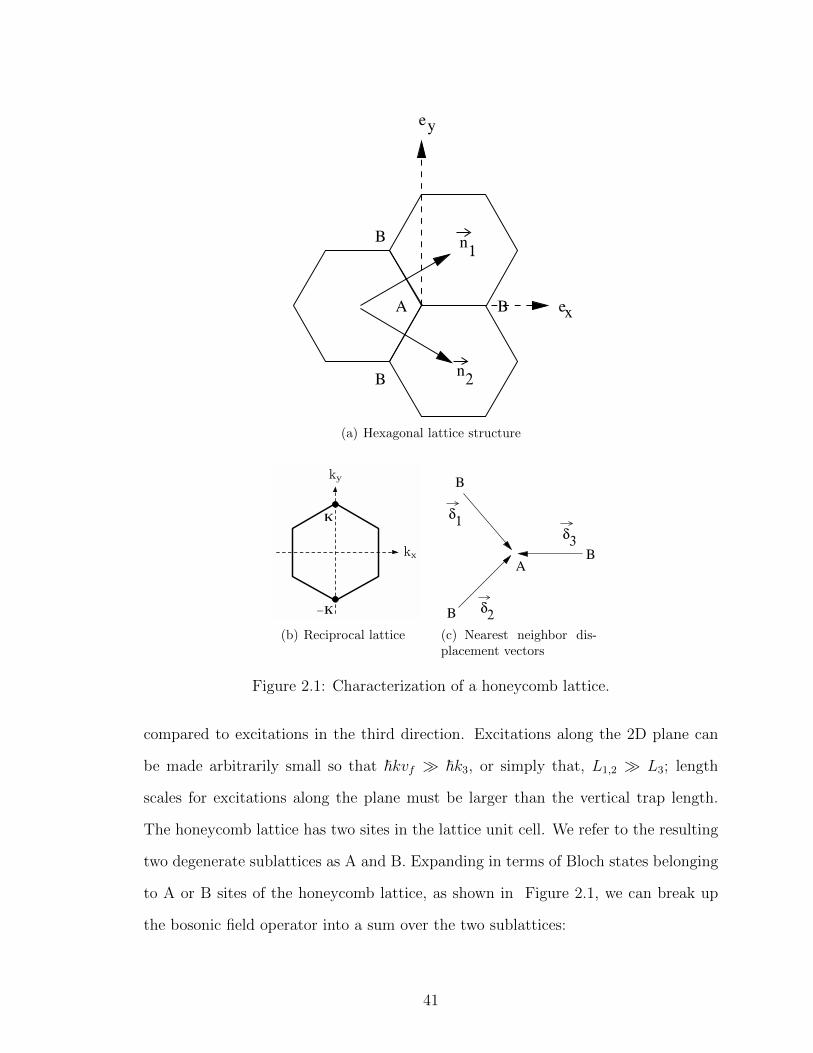
A

e

B

B

B e

n

n

y

x

1

2

(a) Hexagonal lattice structure

K

−K

ky

kx

(b) Reciprocal lattice

AB

B

B

δ

δ

δ

1

3

2

(c) Nearest neighbor dis-placement vectors

Figure 2.1: Characterization of a honeycomb lattice.

compared to excitations in the third direction. Excitations along the 2D plane can

be made arbitrarily small so that ~kvf ~k3, or simply that, L1,2 L3; length

scales for excitations along the plane must be larger than the vertical trap length.

The honeycomb lattice has two sites in the lattice unit cell. We refer to the resulting

two degenerate sublattices as A and B. Expanding in terms of Bloch states belonging

to A or B sites of the honeycomb lattice, as shown in Figure 2.1, we can break up

the bosonic field operator into a sum over the two sublattices:

41

ψ = ψA + ψB , (2.3)

ψA ≡∑A

a ei~k·(~r−~rA)u(~r − ~rA) , (2.4)

ψB ≡∑B

b ei~k·(~r−~rB)u(~r − ~rB) , (2.5)

where a and b are the time-dependent destruction operators at A and B sites re-

spectively and ~rA and ~rB are the positions of A and B sites respectively.The spatial

dependence is then encapsulated outside the operator in the exponential and the func-

tions u. The summation indices indicate sums over A or B sites.Inserting Eq. (9.3)

into Eq. (9.1), the Hamiltonian can be rewritten

H =

∫d2r[(ψ†A + ψ†B)H0(ψA + ψB)

+g

2(ψ†A + ψ†B)(ψ†A + ψ†B)(ψA + ψB)(ψA + ψB)

]. (2.6)

In the integral over H0, imposing the restriction of nearest-neighbor interactions in

the tight-binding, lowest band approximation eliminates all A-A and B-B transitions

except for on-site kinetic and potential terms; the latter can be neglected as an

overall self-energy. Then only integrals involving neighboring A-B sites remain in

the sum. Similarly, in the interaction term only on-site terms are non-negligible, i.e.,

overlap of functions u belonging to the same site. Specifically, the terms dropped

from the summation are integrals of products of four onsite localized wavefunctions

with at least one belonging to a different site than the others. They are of the

form∫d3ru∗0iu

∗0ju0ku0l . Since we are performing all calculations in the tight-binding

approximation we neglect all such terms unless i = j = k = l . Note that the hopping

integral is th = −∫d3ru∗0(r−Ri)H0u0(r−Rj), where i and j refer to nearest neighbor

sites.

Thus in the tight-binding, lowest band approximation, Eqs. (9.4)-(9.5) are substi-

tuted into Eq. (2.6) to yield:

42

H =

∫d2r

∑<A,B>

[a† e−i

~k·~χAu(~χA)H0a ei~k·~χAu(~χA)

+a† e−i~k·~χAu(~χA)H0b e

i~k·~χBu(~χB)

+b† e−i~k·~χBu(~χB)H0a e

i~k·~χAu(~χA)

+b† e−i~k·~χBu(~χB)H0b e

i~k·~χBu(~χB)]

+g

2

∫d2r∑A

a†a†aa [u(~χA)]4

+g

2

∫d2r∑B

b†b†bb[u(~χB)]4 , (2.7)

~χA ≡ ~r − ~rA , ~χB ≡ ~r − ~rB , ~χAB = ~rA − ~rB . (2.8)

Isolating the integrals by pulling out all sums and terms not dependent on ~r, Eq. (9.6)

becomes

H =∑

<A,B>

[a†b ei

~k·~χAB

∫d2re−i

~k·~ru(~χA)H0ei~k·~ru(~χB)

+ b†a e−i~k·~χAB

∫d2re−i

~k·~ru(~χB)H0ei~k·~ru(~χA)

]+∑A

a†a

∫d2re−i

~k·~ru(~χA)H0ei~k·~ru(~χA)

+∑B

b†b

∫d2re−i

~k·~ru(~χB)H0ei~k·~ru(~χB)

+g

2

∑A

a†a†aa

∫d2r[u(~χA)]4

+g

2

∑B

b†b†bb

∫d2r[u(~χB)]4 , (2.9)

Finally, we redefine the spatial integrals in Eq. (9.23) as hopping energy th and inter-

action energy U , respectively, as is standard for the Hubbard Hamiltonian [142, 143]:

H = −th∑

<A,B>

[a†b ei

~k·(~rA−~rB) + b†a e−i~k·(~rA−~rB)

]+U

2

∑A

a†a†aa+U

2

∑B

b†b†bb (2.10)

43

The bracketed A and B summation index signifies a sum over nearest-neighbor A

and B sites. The terms proportional to a†a and b†b just count the total number of

atoms in the system, and have been neglected in Eq. (2.10) as an overall constant.

Equation (2.10) is the Hubbard Hamiltonian divided into two degenerate sublattices

A and B, appropriate to the honeycomb optical lattice.

In order to work towards the nonlinear Dirac equation, we calculate the time

evolution of a and b according to the standard Heisenberg picture prescription. This

is similar to the approach taken by Pitaevskii in his landmark paper which first

obtained the NLSE, or Gross-Pitaevskii equation [59]. The Heisenberg equation of

motion is

i~ ∂tak = [ak, H] . (2.11)

The operator ak, which destroys a boson at site k, satisfies the bosonic commutation

relation

[ak, a†k′ ] = δkk′ . (2.12)

Then the commutator with the on-site interaction terms reduces to

[ak, a†ka†kakak] = aka

†ka†kakak − a†ka†kakakak. (2.13)

Taking the first product on the right and commuting the furthermost left a through

according to Eq. (2.12), one finds

aka†ka†kakak = 2a†kakak + a†ka

†kakakak.

Substituting Eq. (2.14) into Eq. (2.13), one obtains

[ak, a†ka†kakak] = 2a†kakak . (2.14)

Substituting Eq. (2.14) into Eq. (2.11) and the Hubbard Hamiltonian Eq. (2.10), one

finds

44

i~ ∂tak = −th[bk e

i~k·(~rAk−~rBk

) + bk−n1 ei~k·(~rAk

−~rBk−n1)

+bk−n2 ei~k·(~rAk

−~rBk−n2)]

+ Ua†kakak , (2.15)

where the first three terms on the right hand side represent transitions from the

three B-sites nearest the kthsite of the A sublattice and ~n1 and ~n2 are primitive cell

translation vectors for the reciprocal lattice, as shown in Figure 2.1.

In a similar fashion as Eqs. (2.11)-(2.15), we arrive at the an expression of the

same form for the B sublattice,

i~∂tbk = −th[ak e

−i~k·(~rAk−~rBk

) + ak+n1 e−i~k·(~rAk+n1

−~rBk)

+ak+n2 e−i~k·(~rAk+n2

−~rBk)]

+ Ub†kbkbk. (2.16)

Continuing to follow Pitaevskii’s method, we next calculate the time rate of change

of the expectation value of Eqs. (2.15) and (2.16) with respect to on-site coherent

states. A tensor product over sites of such coherent states is also assumed [139]. A

more formal, careful treatment of finite number states, rather than coherent states,

has been worked out in the literature (see [12] and references therein). Either way, we

obtain coupled equations of motion for discrete, on-site, complex-valued amplitudes.

For simplicity of notation we take

ak ≡< ak > , bk ≡< bk > . (2.17)

Inserting the nearest-neighbor vectors ~δ1, ~δ2, and ~δ3 in the exponentials in Eqs. (2.15)

and (2.16), as shown in Figure 2.1, we obtain

i~ ak = −th(bk ei~k·~δ3 + bk−n1 ei~k·~δ1 + bk−n2 e

i~k·~δ2)

+Ua∗kakak , (2.18)

i~ bk = −th(ak e−i~k·~δ3 + ak+n1 e−i~k·~δ1 + ak+n2 e

−i~k·~δ2)

+Ub∗kbkbk , (2.19)

45

where n1 and n2 in the indices label the lattice sites in the two directions of the

primitive-cell translation vectors ~n1 and ~n2.

The NLDE is derived around the linear band crossings between the A and B

sublattices at the Brillouin zone corners [50], called the Dirac cones in the graphene

literature [48]. To this end, we insert particular values for the the nearest-neighbor

displacement vectors ~δ and evaluate ~k at the Brillouin zone corner, defined by ~k =

~K = (0, 4π/3) , ~δ1 = ( 12√

3,−1

2), ~δ2 = ( 1

2√

3, 1

2), ~δ3 = (− 1√

3, 0). Then Eqs. (2.18)-(2.19)

become

i~ ak = −th(bk e0 + bk−n1 e−i2π/3 + bk−n2 e

i2π/3)

+Ua∗kakak . (2.20)

Reducing the exponentials,

i~ ak = −th[bk + bk−n1(−1/2− i√

3/2)

+bk−n2(−1/2 + i√

3/2)] + Ua∗kakak . (2.21)

In anticipation of taking the long wavelength, continuum limit, as is necessary

to obtain the NLDE, we group terms appropriately in order to construct discrete

versions of derivatives. We demonstrate this procedure for Eq. (2.20) only, as it is

identical in form for Eq. (2.21). Grouping terms in Eq. (2.20),

i~ ak = −th[bk + (bk − bk−n1)(1/2 + i√

3/2)

−bk(1/2 + i√

3/2) + (bk − bk−n2)(1/2− i√

3/2)

−bk(1/2− i√

3/2)] + Ua∗kakak , (2.22)

which reduces to

i~ak = −th[(bk − bk−n1)(1/2 + i√

3/2)

+(bk − bk−n2)(1/2− i√

3/2)] + Ua∗kakak . (2.23)

46

At this point it is appropriate to elaborate on the meaning of the c-valued aj and bj

in our derivation. To explain the physics here we borrow from the molecular orbital

model of graphene. In this language we say that the Π-bonding and anti-bonding

orbitals correspond to the valence and conduction bands respectively. Bringing the

system in the vicinity of the Dirac point corresponds to a continuous distortion of

the bonding and ant-bonding orbitals where, at the Dirac point, they become indis-

tinguishable. It is standard in the literature to examine perturbations near the Dirac

point by linearizing the states in momentum space. This we will also do. But our

approach departs from the usual in that we have averaged with respect to coherent

states in the tight-binding limit and are thus effectively left with a theory in position

space where the fundamental length scale is the lattice spacing. Since Eq. (2.23)

results from evaluating our equations at the Dirac point, small perturbations in mo-

mentum correspond to long wavelength modes which involve little change in nearby

aj and bj amplitudes. Since amplitude changes are small on the order of the lattice

spacing we can equivalently recast our equation using continuous functions for the

onsite amplitudes provided the momentum of the perturbation satisfies the condition

that p h/d where h is Planck’s constant and d is the lattice spacing.

Taking the continuum limit and replacing the discrete quantities ak and bk by the

continuous functions ψA = ψA(~r) and ψB = ψB(~r), we arrive at

i~ψA = −th[∂ψB∂n1

(1/2 + i√

3/2) +∂ψB∂n2

(1/2− i√

3/2)

]+Uψ∗AψAψA . (2.24)

where the partial derivatives are in the directions of the unit-cell vectors ~n1 and ~n2.

With a little trigonometry we find that the unit-cell vectors are

~n1 = cos(π/6)ex − sin(π/6)ey =√

3/2ex − 1/2ey , (2.25)

~n2 = cos(π/6)ex + sin(π/6)ey =√

3/2ex + 1/2ey . (2.26)

47

Up to now the “hat” symbol (accent circumflex) has been reserved for operators alone.

However, in Eqs. (2.25)-(2.26) we use this symbol to indicate a unit vector in the x

and y directions. Thus

∂n1 = ~n1 · ~5 = (√

3/2)∂x − (1/2)∂y , (2.27)

∂n2 = ~n2 · ~5 = (√

3/2)∂x + (1/2)∂y . (2.28)

Substituting Eqs. (2.27)-(2.28) into Eq. (2.24),

i~ψA = −t[(√

3/2∂x − 1/2∂y)ψB(1/2 + i√

3/2)

+(√

3/2∂x + 1/2∂y)ψB(1/2− i√

3/2)]

+Uψ∗AψAψA . (2.29)

Further simplification of Eq. (2.29) leads to

i~ψA = −th√

3/2(∂xψB − i∂yψB) + Uψ∗AψAψA (2.30)

Similarly, for the continuum limit of bk → ψB = ψB(~r),

i~ψB = −th√

3/2(−∂xψA − i∂yψA) + Uψ∗BψBψB . (2.31)

Eqs (2.30)-(2.31) are in fact massless Dirac equations with an added nonlinear

term. To put this in a more familiar form, we use Pauli matrix notation. To this end,

one must rename the coordinate axes so that x → y, and, in order to preserve the

handedness of the coordinate system, y → −x. We also reinsert the lattice constant

a; note that a is unrelated to the s-wave scattering length as briefly mentioned in the

definition of g following Eq. (9.1). Thus ∂x → ∂y and ∂y → −∂x. Then Eqs. (2.30)-

(2.31) become

i~ψA = −tha√

3/2(∂yψB + i∂xψB) + Uψ∗AψAψA , (2.32)

i~ψB = −tha√

3/2(−∂yψA + i∂xψA) + Uψ∗BψBψB , (2.33)

48

or in matrix form,

i~(ψAψB

)=−itha

√3

2

(0 ∂x − i∂y

∂x + i∂y 0

)(ψAψB

)+ U

(ψ∗AψAψAψ∗BψBψB

). (2.34)

We can write Eq. (2.34) more compactly in terms of Pauli matrices (σ1, σ2) = ~σ,

i~(ψAψB

)=−itha

√3

2~σ · ~5

(ψAψB

)+ U

(ψ∗AψAψAψ∗BψBψB

). (2.35)

Equation (2.35) is the NLDE. However, we can make one further step by expressing

Eq. (2.35) in a more covariant looking form as follows in (2+1) dimensions:

(iσ0∂t + icl~σ · ~∇)

(ψAψB

)− U

(ψ∗AψAψAψ∗BψBψB

)= 0 , (2.36)

where ~σ and ~∇ are restricted to the x− y plane. In Eq. (2.36),

cl ≡ tha√

3/2~ (2.37)

is an effective speed of light of the condensate in the lattice[144, 145] (in graphene it

would be replaced with the Fermi velocity [48]). This velocity is an effective speed of

light for excitations of the NLDE in our QED2+1 theory. Experimental values of cl

in BECs are on the order of cm/s, ten orders of magnitude slower than the speed of

light in a vacuum. Note also that in Eq. (2.36) U has now absorbed a factor of 1/~.

Finally, a few additional definitions lead to a nicely compact form for the NLDE. Let

A ≡(

1 00 0

), B ≡

(0 00 1

), ψ ≡

(ψAψB

), ψ ≡

(ψ∗A, ψ

∗B

). (2.38)

With the choice of metric which raises and lowers space-time indices restricted to

(2+1) dimensions,

gµν =

1 0 00 −1 00 0 −1

, (2.39)

Eq. (2.36) becomes

49

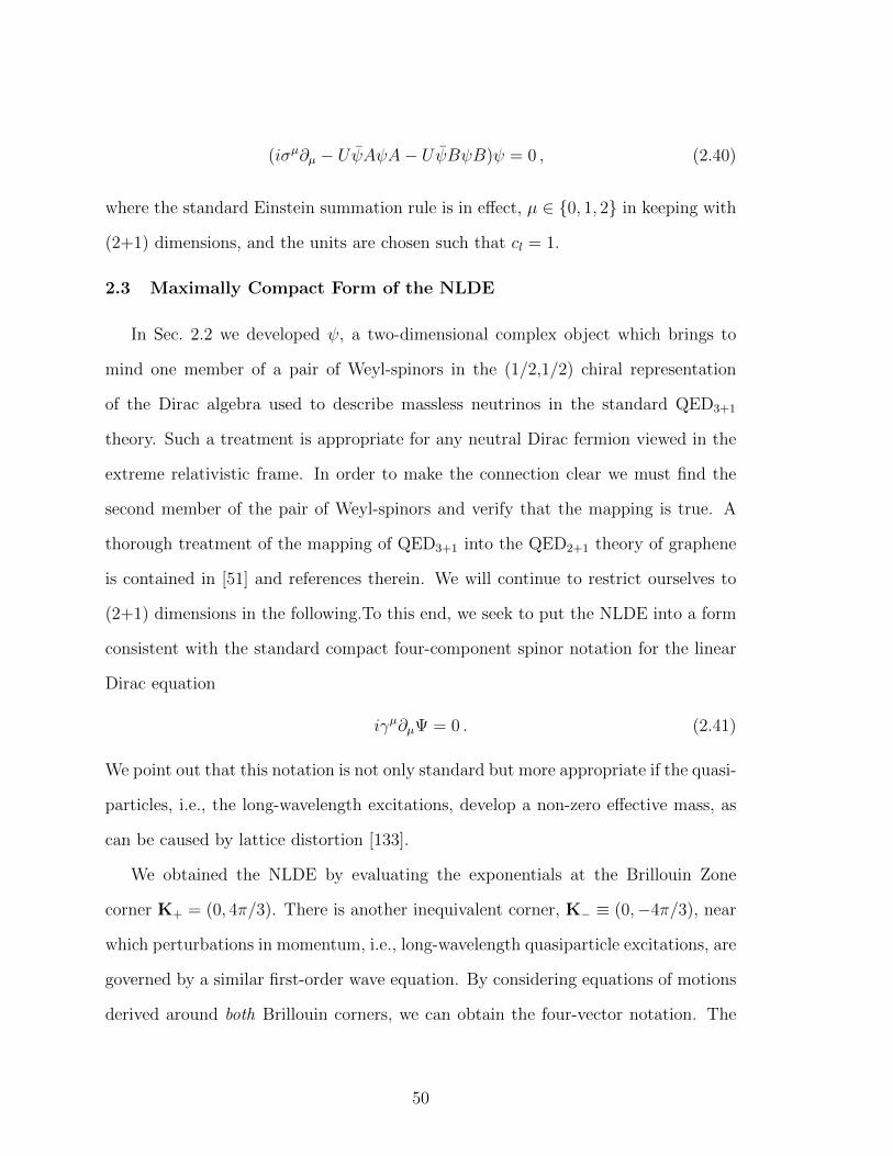
(iσµ∂µ − UψAψA− UψBψB)ψ = 0 , (2.40)

where the standard Einstein summation rule is in effect, µ ∈ 0, 1, 2 in keeping with

(2+1) dimensions, and the units are chosen such that cl = 1.

2.3 Maximally Compact Form of the NLDE

In Sec. 2.2 we developed ψ, a two-dimensional complex object which brings to

mind one member of a pair of Weyl-spinors in the (1/2,1/2) chiral representation

of the Dirac algebra used to describe massless neutrinos in the standard QED3+1

theory. Such a treatment is appropriate for any neutral Dirac fermion viewed in the

extreme relativistic frame. In order to make the connection clear we must find the

second member of the pair of Weyl-spinors and verify that the mapping is true. A

thorough treatment of the mapping of QED3+1 into the QED2+1 theory of graphene

is contained in [51] and references therein. We will continue to restrict ourselves to

(2+1) dimensions in the following.To this end, we seek to put the NLDE into a form

consistent with the standard compact four-component spinor notation for the linear

Dirac equation

iγµ∂µΨ = 0 . (2.41)

We point out that this notation is not only standard but more appropriate if the quasi-

particles, i.e., the long-wavelength excitations, develop a non-zero effective mass, as

can be caused by lattice distortion [133].

We obtained the NLDE by evaluating the exponentials at the Brillouin Zone

corner K+ = (0, 4π/3). There is another inequivalent corner, K− ≡ (0,−4π/3), near

which perturbations in momentum, i.e., long-wavelength quasiparticle excitations, are

governed by a similar first-order wave equation. By considering equations of motions

derived around both Brillouin corners, we can obtain the four-vector notation. The

50

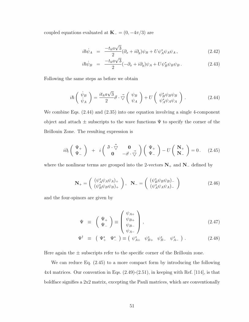
coupled equations evaluated at K− = (0,−4π/3) are

i~ψA =−tha

√3

2(∂x + i∂y)ψB + Uψ∗AψAψA , (2.42)

i~ψB =−tha

√3

2(−∂x + i∂y)ψA + Uψ∗BψBψB . (2.43)

Following the same steps as before we obtain

i~(ψBψA

)=itha√

3

2~σ · ~5

(ψBψA

)+ U

(ψ∗BψBψBψ∗AψAψA

). (2.44)

We combine Eqs. (2.44) and (2.35) into one equation involving a single 4-component

object and attach ± subscripts to the wave functions Ψ to specify the corner of the

Brillouin Zone. The resulting expression is

i∂t

(Ψ+

Ψ−

)+ i

(σ · 5 0

0 −~σ · ~5

)(Ψ+

Ψ−

)− U

(N+

N−

)= 0 . (2.45)

where the nonlinear terms are grouped into the 2-vectors N+ and N− defined by

N+ =

((ψ∗AψAψA)+

(ψ∗BψBψB)+

), N− =

((ψ∗BψBψB)−(ψ∗AψAψA)−

)(2.46)

and the four-spinors are given by

Ψ ≡(

Ψ+

Ψ−

)≡

ψA+

ψB+

ψB−ψA−

, (2.47)

Ψ† ≡(

Ψ∗+ Ψ∗−)≡(ψ∗A+ ψ∗B+ ψ∗B− ψ∗A−

). (2.48)

Here again the ± subscripts refer to the specific corner of the Brillouin zone.

We can reduce Eq. (2.45) to a more compact form by introducing the following

4x4 matrices. Our convention in Eqs. (2.49)-(2.51), in keeping with Ref. [114], is that

boldface signifies a 2x2 matrix, excepting the Pauli matrices, which are conventionally

51

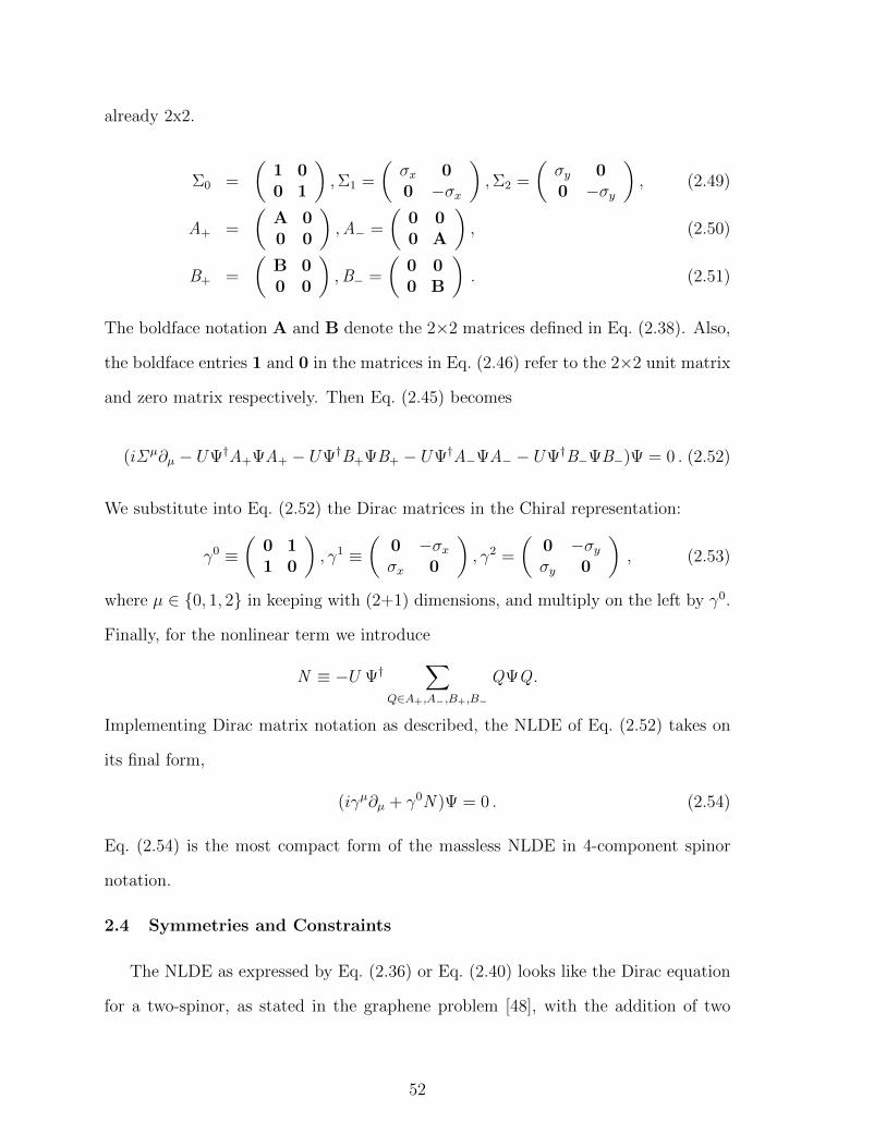
already 2x2.

Σ0 =

(1 00 1

),Σ1 =

(σx 00 −σx

),Σ2 =

(σy 00 −σy

), (2.49)

A+ =

(A 00 0

),A− =

(0 00 A

), (2.50)

B+ =

(B 00 0

),B− =

(0 00 B

). (2.51)

The boldface notation A and B denote the 2×2 matrices defined in Eq. (2.38). Also,

the boldface entries 1 and 0 in the matrices in Eq. (2.46) refer to the 2×2 unit matrix

and zero matrix respectively. Then Eq. (2.45) becomes

(iΣµ∂µ − UΨ†A+ΨA+ − UΨ†B+ΨB+ − UΨ†A−ΨA− − UΨ†B−ΨB−)Ψ = 0 . (2.52)

We substitute into Eq. (2.52) the Dirac matrices in the Chiral representation:

γ0 ≡(

0 11 0

), γ1 ≡

(0 −σxσx 0

), γ2 =

(0 −σyσy 0

), (2.53)

where µ ∈ 0, 1, 2 in keeping with (2+1) dimensions, and multiply on the left by γ0.

Finally, for the nonlinear term we introduce

N ≡ −U Ψ†∑

Q∈A+,A−,B+,B−

QΨQ .

Implementing Dirac matrix notation as described, the NLDE of Eq. (2.52) takes on

its final form,

(iγµ∂µ + γ0N )Ψ = 0 . (2.54)

Eq. (2.54) is the most compact form of the massless NLDE in 4-component spinor

notation.

2.4 Symmetries and Constraints

The NLDE as expressed by Eq. (2.36) or Eq. (2.40) looks like the Dirac equation

for a two-spinor, as stated in the graphene problem [48], with the addition of two

52

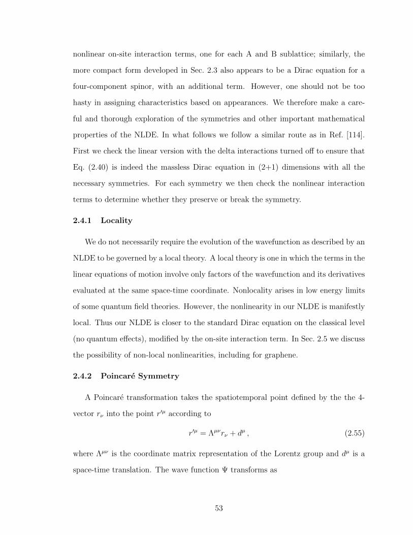
nonlinear on-site interaction terms, one for each A and B sublattice; similarly, the

more compact form developed in Sec. 2.3 also appears to be a Dirac equation for a

four-component spinor, with an additional term. However, one should not be too

hasty in assigning characteristics based on appearances. We therefore make a care-

ful and thorough exploration of the symmetries and other important mathematical

properties of the NLDE. In what follows we follow a similar route as in Ref. [114].

First we check the linear version with the delta interactions turned off to ensure that

Eq. (2.40) is indeed the massless Dirac equation in (2+1) dimensions with all the

necessary symmetries. For each symmetry we then check the nonlinear interaction

terms to determine whether they preserve or break the symmetry.

2.4.1 Locality

We do not necessarily require the evolution of the wavefunction as described by an

NLDE to be governed by a local theory. A local theory is one in which the terms in the

linear equations of motion involve only factors of the wavefunction and its derivatives

evaluated at the same space-time coordinate. Nonlocality arises in low energy limits

of some quantum field theories. However, the nonlinearity in our NLDE is manifestly

local. Thus our NLDE is closer to the standard Dirac equation on the classical level

(no quantum effects), modified by the on-site interaction term. In Sec. 2.5 we discuss

the possibility of non-local nonlinearities, including for graphene.

2.4.2 Poincare Symmetry

A Poincare transformation takes the spatiotemporal point defined by the the 4-

vector rν into the point r′µ according to

r′µ = Λµνrν + dµ , (2.55)

where Λµν is the coordinate matrix representation of the Lorentz group and dµ is a

space-time translation. The wave function Ψ transforms as

53

Ψ′(r ′) = M(Λ)Ψ(r) ,

where the matrices M(Λ) form a representation of the subgroup of the Lorentz group

consisting of spatial rotations and boosts. Boosts can be thought of as rotations

in imaginary time by imaginary angles mixing space and time coordinates. We re-

strict these transformations to (2+1) dimensions. The proof of Lorentz covariance

of the standard massless Dirac equation, Eq. (2.41), is arrived at with the aid of the

transformations for the wave function and partial derivatives

Ψ(r) = M−1(Λ)Ψ′(r′) , (2.56)

∂

∂xi= Λji

∂

∂x′j. (2.57)

This yields the conditions for the Dirac matrices:

γj = ΛjiMγiM−1 . (2.58)

The standard form of the Dirac matrices obtained this way can be found in the

literature [86] and are identical to the results of our theory.

Thus imposing Lorentz covariance on the NLDE as expressed in Eq. (2.54) requires

Ψ to transform under the irreducible representation of a subgroup of SL(2,C), the

2 × 2 complex matrices of unit determinant. The four-dimensional representation

of SL(2,C), D(1/2,1/2), is formed by taking the direct product of the two-dimensional

representations D(1/2,0) and D(0,1/2)

D(1/2,1/2) = D(1/2,0) ⊗D(0,1/2) . (2.59)

This subgroup of SL(2,C) is isomorphic to a subgroup of the Lorentz group, the one

obtained by restricting Lorentz transformations to the plane of the honeycomb lattice.

So, the upper two components of Ψ transform as a spinor under D(1/2,0), the lower two

54

as a spinor under D(0,1/2), and Ψ itself as a four-component spinor or bispinor [146].

The next task is to examine the behavior of Ψ, as defined in Eq. (2.48) and

governed by Eq. (2.54), under rotations in the x−y plane. In order to obtain Poincare

covariance we must show that it is the same as that of a four-component spinor in

the standard Dirac3+1 theory restricted to the 2D plane. The honeycomb lattice is

invariant under rotations by ±2π/3 but the four components of Ψ are also defined

by the particular corner of the Brillouin Zone. Since we’re considering a discrete

lattice it is natural to discuss discrete rotations which realign lattice points and in the

continuum limit map the continuous rotations of QED2+1 onto our theory. Rotations

by ±π/3 exchange A and B sites, and take the theory to that of the opposite ~K point:

~K+ does not go to ~K− but the result after calculating the relative phase exponentials

gives back the same theory. To see this we chose a different primitive unit cell, the

one obtained by a rotation of 2π/3 about the ~n1, ~n2 origin in Fig Figure 2.1. This is

because the direction of ~K ′+ (defined as ~K+ rotated by π/3) differs from that of ~K−

by 2π/3. Thus under this discrete rotation

bk → bk−2n1 , (2.60)

bk−n1 → bk−n1−n2 , (2.61)

bk−n2 → bk−n1 , (2.62)

ak → ak−n1 , (2.63)

ak+n1 → ak−2n1+n2 , (2.64)

ak+n2 → ak−2n1 . (2.65)

Also, we observe that

~K ′+ · ~δ3 = ~K− · ~δ1 (2.66)

~K ′+ · ~δ1 = ~K− · ~δ2 (2.67)

~K ′+ · ~δ2 = ~K− · ~δ3 . (2.68)

Putting these together, we obtain

55

i~ ak−n1 = −th(bk−2n1 ei ~K−·~δ1 + bk−n1−n2 e

i ~K−·~δ2

+bk−n1 ei ~K−·~δ3) + Ua∗k−n1

ak−n1ak−n1 , (2.69)

i~ bk−2n1 = −th(ak−n1 e−i ~K−·~δ1 + ak−2n1+n2 e

−i ~K−·~δ2

+ak−2n1 e−i ~K−·~δ3) + Ub∗k−2n1

bk−2n1bk−2n1 . (2.70)

Now, we redefine the index k: in Eq. (2.69), k → k + n1, while in Eq. (2.70), k →

k + 2n1. Then

i~ ak = −th(bk−n1 ei ~K−·~δ1 + bk−n2 e

i ~K−·~δ2 + bk ei ~K−·~δ3) + Ua∗kakak (2.71)

i~ bk = −th(ak+n2 e−i ~K−·~δ1 + ak+n2 e

−i ~K−·~δ2 + ak e−i ~K−·~δ3) + Ub∗kbkbk. (2.72)

To summarize, a rotation by π/3 which takes ~K+ → ~K ′+ is identical to the un-

rotated theory but with ~K+ → ~K−. Note that the redefinition of the index k is

different for the two equations because old and new primitive cells are related by a

rotation. Rotating by ±2π/3 exchanges A and B sites once more and returns Ψ to

its original configuration. Since Ψ has four components, the effect of making one full

rotation of 2π is that the components acquire a net phase so that Ψ → −Ψ. This

Berry phase [128] endows Ψ with the characteristic double-valuedness of a genuine

4-spinor. However, we must be cautious when discussing chirality and helicity, since

we treat (2+1) dimensions and can use only the first two Pauli matrices. As in the

(3+1) theory, one can define a pseudo-chirality operator in (2+1) dimensions, γ5, as

the product of the other four γ matrices. In the Weyl, or Chiral, representation we

have

γ5 ≡ iγ0γ1γ2γ3 =

(1 00 −1

), (2.73)

where again the boldface indicates a 2x2 submatrix. This is the natural representation

for Ψ in that the NLDE of Eq. (2.54) maps into this representation in a natural way:

states of well defined chirality correspond to the upper and lower 2-spinors. Thus the

56

upper and lower spinors

Ψ+ ≡(ψ+

0

), Ψ− ≡

(0ψ−

)(2.74)

are eigenfunctions of γ5,

γ5Ψ+ = Ψ+ , γ5Ψ− = −Ψ− . (2.75)

The question of Poincare covariance of the nonlinear Dirac equation remains. We

check first coordinate translations. The wave function is required to transform as

Ψ′(r + d) = Ψ(r) . (2.76)

Thus the nonlinear terms which have two factors of Ψ are invariant under translations.

Under spatial rotations we observe that the interaction terms in the NLDE remain

unchanged within the context of the full theory. We include both ~K+ and ~K− points

in the full theory. As for the case of boosts, we note that for the linear equation the

components of the wave function transform in accordance with the transformation

of the space-time coordinates in their arguments. This is exactly canceled by the

reciprocal transformations of the partial derivatives. This is not the case for the

nonlinear terms. One has some matrix product with two factors of the wave function.

Thus the nonlinear Dirac equation is not invariant under Lorentz boosts.

For any truly fundamental theory of nature it is demanded that the governing

equations be invariant with respect to the Poincare group. Sometimes this require-

ment is loosened as in the quantization of gauge theories, when fixing the gauge causes

relativistic covariance to be non-manifest. Yet the theory itself certainly remains in-

variant. Other times the breaking of Poincare covariance implies that we are dealing

with an effective theory in which deeper physical processes are at work. Our case

is an example of the latter. By including on-site interactions we break “relativistic”

invariance of the linear theory by introducing self-interactions which can be viewed

as evidence of “deeper physics” in our two-dimensional universe.

57

2.4.3 Hermiticity

We require the Hamiltonian be Hermitian in order to guarantee that physically

measurable quantities (observables) are real. Thus each term must be independently

Hermitian. In particular, we must show that N † = N . The proof follows:

N † = (UΨ†A+ΨA+)†

= UA†+Ψ†A†+(Ψ†)†

= UA+Ψ † A+Ψ

= UΨ†A+ΨA+

= N , (2.77)

where the last two steps work because A+ is real and symmetric. The nonlinear terms

are indeed Hermitian.

2.4.4 Current Conservation

Current conservation is expected in ordinary QED for a closed system, i.e., an

isolated volume of space. However, most theories of quantum gravity do introduce

Lorentz violating terms which bring in charge non-conservation effects. The conserved

current for the linear Dirac equation is

jµ = ΨγµΨ , (2.78)

where Ψ ≡ Ψ†γ0. We check that this current is also conserved for the NLDE. The

3-divergence of the current in (2+1) spatial dimensions is

∂µjµ = ∂µ(ΨγµΨ)

= ∂µ(Ψ†γ0γµΨ)

= ∂µΨ†γ0γµΨ + Ψ†γ0γµ∂µΨ

= ∂µΨ†γ0γµΨ + Ψ†γ0γµ∂µΨ

= −∂µΨ†γµγ0Ψ + Ψ†γ0γµ∂µΨ , (2.79)

58

where µ ∈ 0, 1, 2 and we have used the anti-commuting properties of the Dirac

matrices. Taking the adjoint of the Dirac equation, Eq. (2.41), yields

(iγµ∂µΨ)† = (−γ0NΨ)†, (2.80)

which implies

−∂µΨ†γµ = −iΨ†N †γ0 . (2.81)

Then the (2+1)-divergence of the current is

∂µjµ = −iΨ†N †γ0γ0Ψ + Ψ†γ0(iγ0NΨ) (2.82)

= −iΨ†(N † −N)Ψ = 0 . (2.83)

Thus current is conserved. This is in fact the statement that hermiticity implies

current conservation.

2.4.5 Chiral Current

The conserved chiral current for the linear Dirac equation is

jµ5 ≡ Ψγµγ5Ψ . (2.84)

Then the (2+1)-divergence of the chiral current is

∂µjµ5 = ∂µ(Ψγµγ5Ψ) . (2.85)

Following a similar route as in Sec. 2.4.4, we find

∂µjµ5 = −iΨ†(Nγ5 + γ5N)Ψ (2.86)

where we have used the hermiticity of N . This means that in order for chiral current

to be conserved we must have

N, γ5 = 0 , (2.87)

where the curly braces signify the anti-commutator. The anti-commutator is

N, γ5 = UΨ†A+ΨA+γ5 + γ5UΨ†A+ΨA+ . (2.88)

59

Writing this out in explicit matrix form we find that

N, γ5 = +2N , (2.89)

N, γ5 = −2N , (2.90)

for the ± subscript terms, respectively. Evidently chiral current is not conserved.

This fact is reminiscent of the anomalous non-conservation of chiral current in the

case of some field theories upon quantization, which is mediated by instantons. It is

interesting to consider that our nonlinear terms might be treated as quantum-induced

nonlinearities.

2.4.6 Universality

Universality refers to the invariance of a theory under rescaling of the solution.

For the case of the linear Dirac equation, Ψ → λΨ leaves the theory unchanged.

Because the nonlinear term in the NLDE contains one factor of Ψ and one factor of

its adjoint, it scales as λ2, thus breaking the invariance of the nonlinear theory. For a

treatment of NLDEs which are universal in this sense, but not relevant to the present

solid state system, see Ref. [114].

2.4.7 Discrete Symmetries

2.4.8 Parity

In the case of the standard massless Dirac equation invariance under a parity

transformation requires Ψ to transform as

Ψ→ Ψ′ = PΨ = γ0Ψ , (2.91)

where, in contrast to the Chiral representation presented in Eq. (2.53), in the Dirac

representation

γ0 =

(1 00 −1

). (2.92)

60

We proceed to determine if the NLDE remains invariant under the transformation

of Eq. (2.91). The parity operator acting on the honeycomb lattice inverts both

coordinate axes, ~∇ → −~∇, and thus exchanges A and B sites while also exchanging

~K-point indices. The transformed linear equations (U = 0) are

iγ0(

Ψ−Ψ+

)+ icl

(−σ · 5 0

0 ~σ · ~5

)γ0(

Ψ−Ψ+

)= 0 . (2.93)

Interchanging upper and lower spinors we obtain the equivalent form

i

(Ψ+

Ψ−

)+ icl

(σ · 5 0

0 −~σ · ~5

)(Ψ+

Ψ−

)= 0 . (2.94)

Thus the linear equations are invariant under the Parity operator. Next we check the

nonlinear term in the NLDE.With the transformed nonlinear term added to Eq. (2.93)

we obtain

i

(Ψ−−Ψ+

)+ icl

(−σ · 5 0

0 ~σ · ~5

)(Ψ−−Ψ+

)− U

(N−−N+

)= 0 , (2.95)

which after similar steps as above gives us back the NLDE. Therefore parity is a

symmetry of the nonlinear Dirac equation. Parity is conserved in standard QED and

also in the theory of the strong interactions, but violated by weak interactions. We

are dealing with a theory which resembles QED and thus in order to reap the benefits

from that theory it is certainly desirable that ours retains parity invariance.

2.4.9 Charge Conjugation

In order to maintain symmetry under charge conjugation one requires the nonlin-

ear term to transform as

(γ0N)′= Cγ0N∗C−1 , (2.96)

where in the chiral representation

61

C = γ1

and the wavefunction transforms in the standard way

Ψ→ γ1γ0Ψ†T. (2.97)

We determine if the NLDE maintains this symmetry. Let F be one of the nonlinear

terms. Then

(γ0N)′

= (γ1γ0Ψ†T

)†A+(γ1γ0Ψ†

T)A+

= ΨTγ0γ1A+γ1γ0Ψ∗A+ (2.98)

Also, we have

Cγ0N∗C−1 = γ1γ0(Ψ†A+ΨA+)∗γ1

= γ1γ0ΨTA+Ψ∗A+γ1 (2.99)

Thus the NLDE breaks charge conjugation symmetry.

2.4.10 Time Reversal

The usual time reversal t→ −t requires that Ψ transform as

Ψ→ Ψ′ = ΘΨ = iγ1γ3Ψ , (2.100)

where Θ is the time-reversal operator and

iγ1γ3 =

(−σy 00 −σy

), (2.101)

In our theory the intrinsic effect of time reversal is to change the direction of momen-

tum so that ~K points are switched without exchanging A and B indices. Combining

these effects, we determine whether or not the linear part of the NLDE, i.e., the linear

Dirac equation, remains invariant:

62

−i ∂∂tiγ1γ3

(Ψ−Ψ+

)+ icl

(σ · 5 0

0 −~σ · ~5

)iγ1γ3

(Ψ−Ψ+

)= 0 (2.102)

Then

−i ∂∂t

(Ψ+

Ψ−

)+ icl

(σ · 5 0

0 −~σ · ~5

)(Ψ+

Ψ−

)= 0. (2.103)

The appearance of the negative sign in front of the time derivative indicates that

these are the equations satisfied by the negative energy solutions, or holes. Thus time

reversal takes the equations describing electrons into holes and those for holes into

electrons but keeps the overall theory invariant. We proceed to consider the nonlinear

term. With the transformed nonlinear term we obtain

−i ∂∂t

(Ψ+

Ψ−

)+ icl

(σ · 5 0

0 −~σ · ~5

)(Ψ+

Ψ−

)− iU

(N+

N−

)= 0 . (2.104)

Here we see that the interaction term has acquired a factor of i so the NLDE is

not invariant under time reversal. Thus, as we see in the standard model of particle

physics, CP and T are not conserved independently but CPT is conserved. A note

on CPT: although it is believed that CPT is a manifest symmetry in nature, charge

conservation, parity, and time reversal may be individually violated under various

circumstances within the standard model of elementary particles. For example, the

theory of neutral kaons violates CP. It would be interesting to investigate how our

theory fits into these special cases of symmetry violation, given that parity and time-

reversal symmetries are maintained while charge conjugation is not.

2.5 Discussion and Conclusions

The nonlinear Dirac equation we have presented introduces a completely new class

of nonlinear phenomena in Bose-Einstein condensates. Although our work is related

to graphene, in that the BEC is taken to be trapped on a honeycomb lattice, we have

63

switched bosons for fermions. The form of the nonlinearity is then a natural physical

result of binary interactions between bosons. In fact, it is a spinor generalization of the

kind of nonlinearity one finds in the nonlinear Schrodinger equation, i.e., proportional

to the local condensate density. The same equation will occur for light subject to

a Kerr nonlinearity when propagating through a photonic crystal with a honeycomb

lattice structure [147–149]. Numerical solutions to these equations should be tractable

using methods discussed in the literature [150–152].

We showed that the NLDE breaks Poincare covariance, and therefore the principle

of relativity. This suggests that small nonlinearities of this form could be looked for

by such symmetry breaking in a variety of systems where Dirac or Dirac-like equations

apply. For instance, even for fermions there is a small mean field effect. We could

just as easily have considered ultra-cold fermions on an optical lattice. This would

appear at first sight to be the exact analog of graphene; however, our work shows

that Poincare covariance will be broken by mean field effects, even if on a small level.

Indeed, for graphene one should expect similar effects due to Coulomb interactions.

The latter nonlinearity can be expected to be non-local due to the power law behavior

of 1/r for the Coulomb potential, just as dipole-dipole interactions between ultra-cold

atoms lead to a non-local nonlinear Schrodinger equation in a 3D continuum (in 2D

dipole-dipole interactions, which have a power law of 1/r3, are local). Thus, in

graphene, we make the conjecture that there is a non-local nonlinear correction term

to the massless Dirac equation which breaks Poincare covariance. Similar corrections

can be looked for in quantum electrodynamics under the proper circumstances [141].

All generalizations of the scalar nonlinear Schrodinger equation relevant to BECs

are candidates for generalized nonlinear Dirac equations. For example, pseudospin

structure leads to a vector NLSE. One can therefore anticipate a vector NLDE as

well.

64

We have thoroughly explored both continuous and discrete symmetries of the

NLDE. In particular, we showed that pseudo-chiral current is not conserved, the

NLDE is not covariant under Lorentz boosts, and it breaks charge conjugation as

well as time reversal symmetry. On the other hand, the NLDE is hermitian, local,

conserves current, and is symmetric under parity. In a future work we will treat soliton

and vortex solutions of the NLDE, as a first step towards a complete classification of

nonlinear relativistic phenomena in BECs.

65

Acknowledgments

We acknowledge useful discussions with Alex Flournoy and Mark Lusk. This work

was supported by the National Science Foundation under Grant PHY-0547845 as part

of the NSF CAREER program.

66

CHAPTER 3

FOUNDATIONAL TOPICS IN THE NONLINEAR DIRAC EQUATION: SPINOR

FORMALISM, SPIN-STATISTICS, LAGRANGIAN ANALYSIS, AND

REDUCTION TO THE NONLINEAR SCHRODINGER EQUATION

3.1 Introduction

Having established the basic foundation of the NLDE, we turn now to several

topics which help understand the physics of the NLDE. Two key questions arise:

first, that the BEC background for the NLDE must acquire properties of a spin-1/2

space, since the geometric phase is a natural consequence of the continuum theory

near a Dirac point. Such phase structure also implies the possibility of non-standard

statistics for quasi-particles. Indeed, quasi-particles in a BEC are collective states,

and need not be bound by the same physical properties of the fundamental constituent

bosons. In our case, we will see that quasi-particles in the NLDE background possess

a non-trivial spin structure and obey fermionic statistics.

Lagrangian analysis provides a deeper understanding of the structure of partial

differential equations in addition to shedding light on the vortex and soliton structure

of a system. In this chapter we construct the classical Hamiltonian for the NLDE,

and use this to derive the Lagrangian by the standard method. Qualitative analy-

sis of the Lagrangian will help us understand the nature of relativistic vortices. We

investigate the classical energy functional approach as well, and determine the struc-

ture of the effective potential and investigate the classical fixed points. Any type of

NLDE should be reducible to some type of NLSE, often the standard cubic form plus

additional correction terms. We derive the NLSE from the NLDE by considering low

67

energy fluctuations in a symmetric background where both spinor components at a

single Dirac point are equal, |δψB|2 ' |δψA|2, but with an extreme asymmetry in

the fluctuations, i.e., |δψB,t|2 |δψA,x|2. Solitons in the 1D case are obtained and

analyzed, as well as quantized vortices for the 2D case.

In addition to the topics above, we present a review of basic spinor theory and

interpret this in the context of the honeycomb lattice. We also present a study of the

behavior of the nonlinearity of the NLDE under Lorentz transformations.

3.2 The Spin-Statistics Theorem and Honeycomb Lattice Elementary Ex-citations

The physics of particles in (2+1)-dimensions is unique in that collective states may

exhibit drastically different properties than their constituent particles. Total wave-

functions may acquire fractional phase values (fractional statistics) upon interchange

of pairs of particles. Particles which exhibit such behavior are known as anyons,

with the term semion reserved for the special case of half-integer multiples of π ac-

cumulated upon interchange. This phenomenon may be interpreted within a basic

quantum mechanical picture as well as at the level of relativistic field theory. The

effect may be illustrated using a simple path integral picture in which exchange of two

particles involves a braiding of paths in configuration space. The key point is that in

(2 + 1)-dimensions, a particular configuration of a given winding cannot be smoothly

deformed into another so that the number of windings involved places many-particle

states into topological classes. The relative phase winding which distinguishes one

particular topological state from another need not be integer valued [153].

To illustrate this at the field theory level we start with a few general assumptions

and provide only a sketch, where specific details may be found in Ref. [153]. The main

assumption is that we work in a (2+1)-dimensional space-time with a field possessing

conserved current, i.e., with a vanishing 4-divergence, and that we examine only

the long-wavelength physics. At the level of the action the reduced dimensionality

68

restricts the types of terms which may appear, the conserved current condition means

that the field may be expressed as the curl of some gauge field, and restricting to long

distances allows one to omit more complicated higher order derivative terms from

the model. The dynamics of the gauge field then appears as a Chern-Simons term

with the usual form of a product of gauge field and derivative. The Chern-Simons

term in (2+2)-dimensions is an example of a topological field theory for which certain

invariant quantities may be computed independent of the particular form of the gauge

field. This means that integrating over the curvature 2-form, for example, of the gauge

bundle (the strength of the gauge field) reduces to a topological invariant, a number

which describes the configuration of the field at spatial infinity, where the space is

homeomorphic to S1. Such invariants correspond to vortex configurations of the gauge

field, specifically the phase winding, which may endow the particle with a fractional

charge or fractional exchange statistics. If in addition, we add a scalar field to our

model, and couple this to the Chern-Simons field, the resulting low-energy effective

theory obtained by integrating out either the gauge field or the scalar field returns

us to a Chern-Simons theory for the dressed scalar or gauge field. This method of

trading one theory for an alternative perspective, the dressed scalar or the dressed

gauge perspective, constitutes a duality. The work of Seradjeh and Franz [154], and

Ryu et. al. [155], provide concrete realizations of these concepts for graphene-like

systems.

The phenomenon of non-standard exchange statistics may be treated within the

framework of differential topology, using the theory of fiber bundles with connec-

tions. Letting (E, π,M, F,G) be a fiber bundle with typical fiber F (more compactly

E π−→M), the differentiable manifolds E and M are the total space and base space,

respectively, π : E −→ M defines a surjection called the projection from the total

space to the base space, and the Lie group G is the structure group acting on the fiber

F . In physics the fiber at a point of the base space p ∈M , denoted by Fp, is usually

69

taken to be either a real vector space, Fp ∈ Rn, with structure group GL(n, R) as

in the case of the tangent bundle TpM ; a complex vector space, Fp ∈ Cn, with

structure group GL(n, C); or a vector space whose elements form a spinor represen-

tation of the spin group, Fp ∈ Spin(n), the universal covering group of SO(n).

The structure group maps the fiber Fp into the neighboring fiber Fp′ isomorphically

through what are called transition functions, whose values are taken in the structure

group. The process of smoothly patching together neighboring fibers is specified by

the particular form of the local transition functions and may lead to interesting non-

trivial global topological structure such as fractional statistics. As we shall see, this

is what happens in the case of long-wavelength excitations of a BEC in a honeycomb

lattice where quasi-particles obey fermionic statistics to first order in the particle

interactions.

The connection between spin and statistics arises naturally in our study of the

BEC with Dirac points. We will see that the bi-partite structure of the honeycomb

lattice endows the condensate wavefunction with a geometric phase, or Berry phase,

so that a spinor formulation becomes necessary as is quite familiar from the study of

electrons in graphene. The presence of a geometric phase endows the condensate with

a non-trivial topological structure and has a direct effect on low-energy quasi-particle

statistics. We can see how this works by taking a path integral point of view which

shows that the condensate splits into topologically distinct sectors corresponding to

different numbers of windings taken between two localized states (vortices). More-

over, this topological structure is only a feature of the continuum limit theory where

energies are infinitesimal compared to the characteristic energy of the lattice scale. It

is easy to see that as long as the coordinate exchange of two states involves smooth,

slowly varying paths which remain within the continuum regime, there will be no

ambiguity regarding the net accumulated phase for that particular exchange process.

We find that quasi-particles obey fermionic statistics even though the fundamental

70

constituents are bosons.

The Berry phase associated with a rotation in the plane has a significant conse-

quence for correlators involving pairs of quasi-particle operators. To illustrate this, we

define the quasi-particle operator φ ≡∑j(uj− v†j), where uj (u†j) and vj (v†j) destroy

(create) quasi-particles in the spinor states uj ≡ (uj,A, uj,B)T and vj ≡ (vj,A, vj,B)T ,

respectively. In a field theory formulation, these operators become quantum fields

whose Lagrangian is given by,

L =

∫d3r Φ (γµ∂µ · 1−M) Φ, (3.1)

where we have concatenated the spinors into one structure, Φ ≡ (u, v), and indi-

cated the expanded space by the unit operator. The matrix M contains the interaction

terms proportional to the particle interaction U in addition to the terms proportional

to µ±Ej, where µ is the chemical potential of the BEC and Ej are the quasi-particle

eigenenergies. The “mass” term in Eq. (3.40) is not Lorentz invariant but accumu-

lates an extra term, under a Lorentz transformation, proportional to U2 which comes

from the transformation properties of the |ΨA(B)|2 factors in M. Thus, to first or-

der in U , L is Lorentz invariant. Now, consider the vacuum-to-vacuum correlation

function 〈0|Φ(r)Φ(r′)|0〉 where r and r′ are the (2 + 1)-dimensional space-time coor-

dinates for two quasi-particle excitations. By analytic continuity, a spatial rotation is

equivalent to one involving time since our theory is CPT invariant [52]. This means

that a change in the order of the fields inside the correlation function is equivalent to

exchanging the spatial positions of r and r′ which gives an extra factor of −1 from the

geometric phase. In essence, the spin-statistics theorem allows us to identify time-

reordering with spatial exchange in the plane which then ties the operator algebra to

the geometric phase [156–159]. We can then deduce the anti-commuting property for

quasi-particles,

71

〈0|Φ(r)Φ(r′) + Φ(r′)Φ(r)|0〉 = 0. (3.2)

Equation 3.2 is the canonical commutation relation for fermions, which holds to first

order in the interaction U .

3.3 Spinor Formalism in the Dirac Equation

In the following analysis we present a review of the basic theory of the Dirac

equation and a physical lattice interpretation of Dirac spinors.

3.3.1 Energy Versus Chiral Representation

The Dirac equation was orignally solved in the Dirac basis for a free particle of

mass m in the form

p0 Φ(x) = ~σ · ~p χ(x) +mΦ(x) (3.3)

p0 χ(x) = ~σ · ~pΦ(x)−mχ(x), (3.4)

where Φ and χ are 2-component spinors: the positive and negative energy 2-spinors

respectively. This is also called the energy representation because each 2-spinor is a

pure positive or negative energy state. For a massless particle these become

p0 Φ(x) = ~σ · ~p χ(x) (3.5)

p0 χ(x) = ~σ · ~pΦ(x). (3.6)

For a particle with 4-momentum (E , ~p) the solutions are (apart from a normalization

factor)

ψ1 = e i( ~p · ~r − E t)

10pzE

px+ipyE

, ψ2 = e i( ~p · ~r − E t)

01

px−ipyEpzE

, (3.7)

72

ψ3 = e− i( ~p · ~r − E t)

pzE

px+ipyE

10

, ψ4 = e− i( ~p · ~r − E t)

px−ipyE−pzE

01

, (3.8)

where Φ and χ are the upper and lower 2-spinors respectively and it should be noted

here that they are not helicity eigenstates. ψ1 and ψ2 are the positive energy solutions

and ψ3 and ψ4 are the negative energy solutions. We get a different form for the 2-

spinor equations (3) and (4) if we instead use the chiral representation for the Dirac

matrices from the start. We then obtain

p0 ΨR(x) = ~σ · ~pΨR(x) (3.9)

p0 ΨL(x) = −~σ · ~pΨL(x) . (3.10)

The subscripts here are used to emphasize that these 2-spinors are in fact helicity

eigenstates. Now we arrive at the form of the equations we first derived for the linear

Dirac equation in graphene where equations identical to (9) and (10) were obtained

(if pz = 0) for K+ and K− corners of the Brillouin zone respectively. Recalling the

identification

ΨR = Ψ+ =

(ψA+

ψB+

)(3.11)

and,

ΨL = Ψ− =

(ψB−ψA−

). (3.12)

Now we find the plane wave solutions to be

p0

(ψA+

ψB+

)= ~σ · ~p

(ψA+

ψB+

), (3.13)

p0

(ψB−ψA−

)= −~σ · ~p

(ψB−ψA−

). (3.14)

73

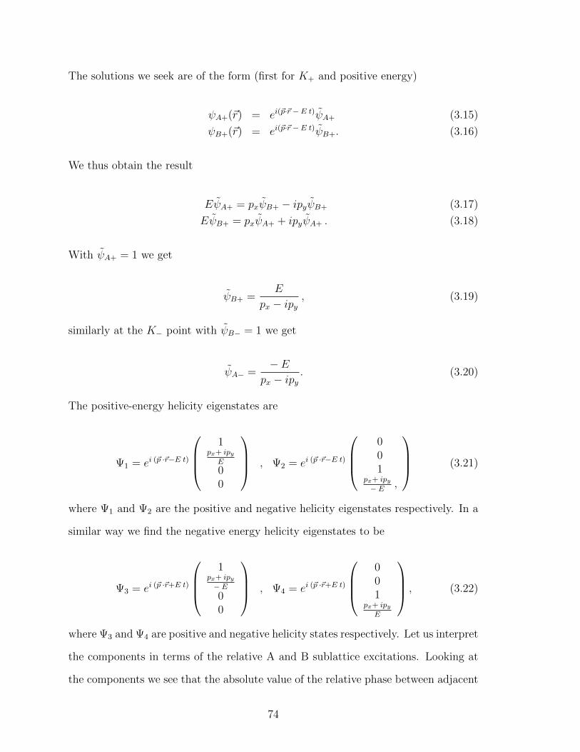
The solutions we seek are of the form (first for K+ and positive energy)

ψA+(~r) = ei(~p·~r − E t)ψA+ (3.15)

ψB+(~r) = ei(~p·~r − E t)ψB+. (3.16)

We thus obtain the result

EψA+ = pxψB+ − ipyψB+ (3.17)

EψB+ = pxψA+ + ipyψA+ . (3.18)

With ψA+ = 1 we get

ψB+ =E

px − ipy, (3.19)

similarly at the K− point with ψB− = 1 we get

ψA− =− E

px − ipy. (3.20)

The positive-energy helicity eigenstates are

Ψ1 = ei (~p ·~r−E t)

1

px+ ipyE

00

, Ψ2 = ei (~p ·~r−E t)

001

px+ ipy− E ,

(3.21)

where Ψ1 and Ψ2 are the positive and negative helicity eigenstates respectively. In a

similar way we find the negative energy helicity eigenstates to be

Ψ3 = ei (~p ·~r+E t)

1

px+ ipy− E00

, Ψ4 = ei (~p ·~r+E t)

001

px+ ipyE

, (3.22)

where Ψ3 and Ψ4 are positive and negative helicity states respectively. Let us interpret

the components in terms of the relative A and B sublattice excitations. Looking at

the components we see that the absolute value of the relative phase between adjacent

74

A and B sites is the same for positive and negative energies but the sign is opposite.

This can be understood by thinking about the shape of the wavefunctions as we tune

the lattice momentum away (increasing) from the corner of the Brillouin zone. In the

state that was the conduction state (when k is slightly less than K+) the relative phase

between A and B sublattices continues to decrease (lowering its energy) while for the

state that was the valence state the opposite is true. But looking at the components of

Ψ1 and Ψ3 this is not what we see: the relative phase φ (comparing the components

1 and (px + ipy)/E we see that tanφ = py/px for Ψ1) becomes more negative for

one state and more positive for the other but is always equal in magnitude. This is

because φ measures the relative phase from the perspective of the reset zero point of

momentum, ie. K-point, or equivalently relative phase between A and B sublattices.

In (21) and (22) we see the symmetry between the chiral 2-spinors that comprise

the upper and lower parts of these solutions: in terms of the 2-spinors, exchanging K+

and K− points has the same effect as changing the sign of the energy. This is certainly

familiar from Standard Model physics since a neutrino with positive helicity can be

viewed as an anti-neutrino with negative helicity moving in the opposite direction.

How do we interpret this in terms of excitations of the A and B sublattices? For a

given k (K+ or K−) and ordering of phase (positive energy or negative energy), if we

simply take K+ to K− then we will have the opposite ordering of phase (relative to

the orientation of the new k value) and so to preserve the state we can simply then

switch the ordering of phase by taking E to −E. Or simply that a quasi-particle with

energy E propagating in the positive direction originates from the same branch of the

spectrum as its antiparticle with energy −E propagating in the opposite direction.

3.3.2 Lorentz Non-Covariance of the NLDE

Here we check the Lorentz transformation properties of the nonlinear term of the

NLDE. The nonlinear terms in the NLDE are

75

γ0UΨ†(rµ)∑

Q∈A+,A−,B+,B−

QΨ(rµ)Q . (3.23)

In order to maintain Lorentz covariance any additional terms to the standard Dirac

equation must form contractions in space-time indices in such a way as to result in

Lorentz scalars; these are by definition the invariant objects under Lorentz transfor-

mations: any factors of gamma matrices must have their space-time indices contracted

with other gamma matrices or with the space-time derivatives and any factors of Ψ

must be contracted as ΨΨ where Ψ = Ψ†γ0. The bilinear terms in our equation are

not independently, nor taken together, the contraction of two Lorentz 4-vectors. Let

us develop this more thoroughly starting with the linear Dirac equation for a particle

of mass m. Using the notation and approach taken in Bjorken and Drell we can show

that under a Lorentz transformation the Dirac equation becomes

[i~S(a)γµS−1(a)aνµ

∂

∂xν ′−mc

]ψ′(x′) = 0 . (3.24)

We arrive at this expression by inserting the Lorentz transformed wavefunction,

ψ(x) = S−1(a)ψ′(x′) , (3.25)

and the transformed partial derivatives where the aνµ are the Lorentz transformation

matrices for coordinates and S(a) are the transformation matrices acting on the

components of the wavefunction induced by the aνµ. Next we left multiplying by S(a).

The purpose behind this step is to keep the mass term in an explicitly invariant form

since we know that the mass does not change under a Lorentz transformation. The

prime on the coordinates indicates the Lorentz transformed coordinates but we must

also allow for the mixing of the components of the wavefunction under a Lorentz

transformation thus ψ(x) → ψ′(x′). From this we see that in order for the Dirac

equation to have the same form in the transformed frame it must be that

76

S(a)γµS−1(a)aνµ = γν . (3.26)

Note that if we contract both sides using the Lorentz transformations we get

S(a)γµS−1(a)aνµ aνσ = γνaν

σ (3.27)

or,

S(a)γµS−1(a)δµσ = γνaν

σ (3.28)

⇒ S(a)γσS−1(a) = γνaνσ . (3.29)

This expresses the property that a Lorentz transformation of the γ matrices from

the point of view of the matrix indices (the left hand side) is equivalent to a Lorentz

transformation on the space-time indices using the space-time matrices aνµ: the γ’s

form a 4-vector with respect to their space-time indices.

Since the transformed γ matrices must still obey the same Clifford algebra (the

same anti-commutation rules) it can be shown that they must be related to the

untransformed γ’s by a unitary transformation thus we leave the right hand side

unprimed. By working from the infinitesimal proper Lorentz transformations we can

get the form for finite transformations S(a)

ψ′(x′) = Sψ(x) = exp

(− i

4ωσµνI

µνn

)ψ(x) . (3.30)

Here Iµνn is the 4x4 space-time matrix for a unit Lorentz rotation about the axis in

the direction labeled n and the σµν are given by σµν = i2

[γµ, γν ]. Also, the Lorentz

rotation angle or rapidity is defined in terms of the relative velocity by tanh(ω) = v/c.

Now let us see what happens when we return to our problem. In our NLDE we

have no mass term but four nonlinear terms. Let us focus on one of the nonlinear

77

terms. By following the steps above we see that the first nonlinear term transforms

like

γ0Ψ†(x)A+Ψ(x)A+ → Sγ0Ψ′†(x′)(S−1)†A+S

−1Ψ′(x′)A+S−1 . (3.31)

These two expressions do not have the same form. The A+ matrices in the untrans-

formed term have the effect of picking out the first element of Ψ and leaving zeros

for the other elements so that in the end there are no mixed products of components

in any of the nonlinear terms. The transformed expression, on the other hand, is a

complicated mixing of components of Ψ′(x′). In particular we see that since S−1 is

itself a Lorentz transformation, the effect of multiplying Ψ′(x′) by A+S−1 (in the full

equation) is not to simply pick out the first element of Ψ′(x′) (as was the case for A+

acting on Ψ), but here instead A+S−1Ψ′(x′) results in a column vector whose first

element is a mixture of all the elements of Ψ′(x′) where the exact form of the mixed

term is determined by the specific choice of Lorentz rotation angle in S−1.

As an example let us see what happens when we apply a Lorentz boost in the

positive x-direction. Then,

S−1Ψ′(x′) = exp

(i

2ωσ01

)Ψ′(x′) , (3.32)

where we compute in the chiral representation

σ01 =i

2[γ0, γ1] (3.33)

= − i2

[γ0, γ1

](3.34)

= −(σx 00 −σx

). (3.35)

Back substituting, expanding the exponential, separating and regrouping even and

odd power terms we get

78

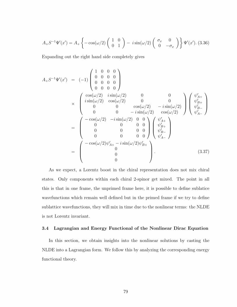
A+S−1Ψ′(x′) = A+

− cos(ω/2)

(1 00 1

)− i sin(ω/2)

(σx 00 −σx

)Ψ′(x′). (3.36)

Expanding out the right hand side completely gives

A+S−1Ψ′(x′) = (−1)

1 0 0 00 0 0 00 0 0 00 0 0 0

×

cos(ω/2) i sin(ω/2) 0 0i sin(ω/2) cos(ω/2) 0 0

0 0 cos(ω/2) − i sin(ω/2)0 0 − i sin(ω/2) cos(ω/2)

ψ′A+

ψ′B+

ψ′B−ψ′A−

=

− cos(ω/2) −i sin(ω/2) 0 0

0 0 0 00 0 0 00 0 0 0

ψ′A+

ψ′B+

ψ′B−ψ′A−

=

− cos(ω/2)ψ′A+ − i sin(ω/2)ψ′B+

000

. (3.37)

As we expect, a Lorentz boost in the chiral representation does not mix chiral

states. Only components within each chiral 2-spinor get mixed. The point in all

this is that in one frame, the unprimed frame here, it is possible to define sublatice

wavefunctions which remain well defined but in the primed frame if we try to define

sublattice wavefunctions, they will mix in time due to the nonlinear terms: the NLDE

is not Lorentz invariant.

3.4 Lagrangian and Energy Functional of the Nonlinear Dirac Equation

In this section, we obtain insights into the nonlinear solutions by casting the

NLDE into a Lagrangian form. We follow this by analyzing the corresponding energy

functional theory.

79

3.4.1 Lagrangian Analysis

Before we obtain exact vortex solutions to the nonlinear Dirac equation it is helpful

to study the theory at the Lagrangian level in order to gain insight into the underlying

principles as well as acquire a qualitative sense of the kinds of solutions to expect.

The nonlinear Dirac equation for the components of a two-spinor is

i ψA,t + i~cl(∂x − i∂y)ψB − U |ψA|2 ψA = 0 (3.38)

i ψB,t + i~cl(∂x + i∂y)ψA − U |ψB|2 ψB = 0 . (3.39)

These are the Euler-Lagrange equations to the Lagrangian density

L = (3.40)

i (ψ∗AψA + ψ∗BψB)t + i~cl [ψ∗A(∂x − i∂y)ψB + ψ∗B(∂x + i∂y)ψA]− U

2(|ψA|4 + |ψB|4) ,

where Eqs. (3.38)-(3.39) are obtained through the prescription

∂µ

(δLδψ∗A,µ

)+

δLδψ∗A

= 0 . (3.41)

The positive sign on the second term is correct, since we are taking functional deriva-

tives with respect to the conjugate of the field and it’s derivatives. The more common

approach is to differentiate the Lagrange density with respect to the field and it’s

derivatives and take the conjugate of the resulting equations afterwards. This leads

to the same result. Eq.(3.40) describes the dynamics of two self-interacting, scalar,

bosonic fields coupled through the spatial derivative terms with interaction strength

strength U and cl is the characteristic speed. The Hamiltonian density can be derived

using the formula

H = πAψA,t + πBψB,t − L , (3.42)

80

where πA and πB are the canonical momenta associated with ψA and ψB respectively.

These are defined in the usual way:

πj =δLδψj,t

, (3.43)

where j labels the field, A or B sublattice in our theory. We get,

H = −i~clψ∗A(∂x − i∂y)ψB − i~clψ∗B(∂x + i∂y)ψA +U

2(|ψA|4 + |ψB|4). (3.44)

Returning to the Lagrangian, in plane polar coordinates it is

L = i (ψ∗AψA + ψ∗BψB)t + i~cl[ψ∗Ae

iθ(∂r − i1

r∂θ)ψB + ψ∗Be

−iθ(∂r + i1

r∂θ)ψA

]−U

2(|ψA|4 + |ψB|4). (3.45)

For static (time-independent) classical solutions, and for strong interactions, we may

write

L = (3.46)

U

[i~clUψ∗Ae

iθ(∂r − i1

r∂θ)ψB + i

~clUψ∗Be

−iθ(∂r + i1

r∂θ)ψA −

1

2(|ψA|4 − |ψB|4)

].

A qualitative analysis of this expression tells us that for U large and attractive (|U |

~cl, U < 0), the quartic interactions dominate and the fields minimize their energy by

forming regions of high density. For a normalized field, this is best done by forming

single solitons. In a dynamic sense, the kinetic terms become costly as the forming

soliton becomes more condensed and the field gradient increases sharply. The minimal

solution may find a stable point in field space by staggering one field with the gradient

of the other ψA > 0, ψB,x < 0 so that the the kinetic terms help to further lower the

energy. This describes a bright vortex/soliton pair configuration for the two spinor

components. We must be careful though in our claim that |U | ~cl, since cl contains

the lattice spacing a, we must impose a more stringent restriction: specifically that

81

|U | th. The reason for this is that the mean field equations that we want to solve

are only valid so long as we are in the quasi-particle domain, i.e., wavelengths that

are large compared to the lattice spacing.

For the case where U is large and repulsive and assuming a finite two-dimensional

box with the usual normalization conditions, the contact interaction is always positive

where the field strength is non-vanishing and the tendency is for the condensate to

lower it’s energy by finding the most favorable combination of fields and gradients that

forces the kinetic terms to be negative. The formation of a local region with large

spatial variation in the fields on an otherwise uniform positive energy background

describes a dark vortex/soliton pair. It may also be energetically favorable for the

condensate to develop a multitude of such configurations, close enough spatially, so

that the moduli of the fields oscillate in some spin texture pattern. This type of

arrangement describes a skyrmion texture.

More generally, we may seek stationary solutions with characteristic energy ~ω.

These are not necessarily ground states of the theory. Time derivatives in the La-

grangian in Eq. (3.45) get replaced by multiplication by −iω so that we have

L = ω(|ψA|2 + |ψB|2

)− (3.47)

i~cl[ψ∗Ae

iθ(∂r − i1

r∂θ)ψB − ψ∗Be−iθ(∂r + i

1

r∂θ)ψA

]− U

2(|ψA|4 + |ψB|4) .

Uniform solutions are possible and obtained by setting the derivatives terms to zero.

The Hamiltonian density for these states is

H =U

2(|ψA|4 + |ψB|4). (3.48)

This is just the field theory representation for uniform density, single particle states

with energy

82

EA = ω =U

2|ψA|4 , (3.49)

EB = ω =U

2|ψB|4 (3.50)

⇒ |ψA|2 = |ψB|2 =

√2 ω

U. (3.51)

Let us look at small fluctuations of these spatially uniform stationary states. To

do this, we can substitute the ansatz ψA = e−iωtvA(r, t) and ψB = e−iωtvB(r, t) in

Eq. (3.45), where ~ω is the energy of the uniform background field density, and,

L = ω|vA|2 + iv∗AvA,t + ω|vB|2 + iv∗BvB,t (3.52)

+ i~clv∗Aeiθ(∂r − i1

r∂θ)vB + i~clv∗Be−iθ(∂r + i

1

r∂θ)vA −

U

2(|vA|4 + |vB|4) .

The Hamiltonian density for the fields vA and vB is given by

H = −i ~ clv∗Aeiθ(∂r − i1

r∂θ)vB − i~clv∗Be−iθ(∂r + i

1

r∂θ)vA

− ω (|vA|2 + |vB|2) +U

2(|vA|4 + |vB|4) . (3.53)

The potential energy density for vA is

PEA = −ω |vA|2 +U

2|vA|4 . (3.54)

Decomposing vA in terms of it’s amplitude and phase, vA =√ρA e

iφA , as expected,

we see that the ground states lie at the minima of (3.54)

vA,0 =

√ω

UeiφA . (3.55)

The ground state is infinitely degenerate parametrized by the phase φA. An identical

result occurs for the other spinor component vB.

83

As with the simplest model of a field theory with broken symmetry, φ4 theory

in two spatial dimensions, our theory admits solutions with topologically nontrivial

structures whose phase winds around the boundary at spatial infinity. Stable states

are then characterized by an integer winding number. We should note that these

two-dimensional vortices do not have finite energy as we shall soon show, and that

the total energy diverges logarithmically consistent with Derrick’s theorem. Luckily

this problem can be handled by introducing an outside gauge potential that couples

to the vortex and conveniently cancels the infinite part of the vortex energy. Thus a

divergent global vortex in (2 + 1)-dimensions is rendered finite when promoted to a

gauged vortex theory.

Physically, the result that we have found here is easy to understand. We could

think of starting with a spatially uniform stationary state with total energy ω, and

adding a small local perturbation to it. The perturbation does not run away because

of the repulsive self-interaction (the outside slope of the Lagrangian potential term),

nor does it collapse due to the local support of the ambient non-zero background

(the inside slope of the potential). Another more interesting scenario is when the

correction to the uniform field cannot be accessed by perturbations but is itself a

topologically stable excited state whose phase wraps around the circle at infinity so

that a zero point of the nonuniform part of the field must exist where the unwrapping

of the phase occurs. These are the vortex solutions that we have already discussed.

3.4.2 Energy Functional Analysis for Relativistic Vortices

We can obtain map of the energy landscape for a vortex configuration by elim-

inating the angular dependence in the energy functional that gives the NLDE as a

variational extremum and then identifying the effective potential energy. If we as-

sume the vortex/soliton form ψA = i e−iθ F (r), ψB = G(r), then the total energy is

given by

84

E =

∫ R

0

dr [−~cl FG′ + ~clGF ′ + Veff(F,G)] , (3.56)

where,

Veff ≡ µ2

2U

(U

µF 2 − 1

)2

+µ2

2U

(U

µG2 − 1

)2

+ ~clGF

r− µ2

U+ µN . (3.57)

We regulate the energy by introducing an upper cutoff R. Evidently the FG′ and

GF ′ terms indicate an attractive force for configurations where sgn(FG′) > 0 and

sgn(F′G) < 0 respectively. In the F,G-plane the centripetal term in Veff dominates

for small r and forms a saddle point at the origin (of the F,G-plane) becoming

singular when r = 0. Because of the saddle-point, points on the F and G axes have

zero potential energy but are unstable. If we want to study solutions that begin at

the saddle-point, i.e., F (0) = G(0) = 0, or on the G-axis, say, near the saddle-point,

we must include the full contribution from the kinetic terms. In fact, we see that a

path in the G-axis defined by p(t) : = t eG, 0 < t < tf , will change the total energy

by ∆E = cltf F′(0). This can be made arbitrarily large and negative by adjusting

the value of F ′ at r = 0. The V -landscape flattens rapidly as r increases from zero

so that it may be possible to attempt a solution for which F (0) = 0, F ′(0) < 0,

and G(0) > 0. For large r, F ′ and G′ must go to zero and the centripetal term

becomes negligible so that Veff has nine extrema, two of which are absolute minima

for the total energy E. The absolute minima occur at the points P and P ′ given by

P (G,F ) = (− q, q) and P ′(G,F ) = (q,−q) where we define q > 0. To determine the

value of q, we can differentiate Eq.(3.57) and solve for minima in the usual manner.

We then expect one of the stable solutions to start at F (0) = 0 , G(0) > 0 and

approach F (∞) = − q , G(∞) = q and the other so start at F (0) = 0, G(0) < 0

and approach F (∞) = q, G(∞) = − q. These describe a bright soliton at the core

of a vortex where the soliton approaches a non-zero value for large r. We obtain the

85

following asymptotic (large r) critical points for Veff in the F,G-plane:

• (√µ/U,

õ/U) - local minimum

• (√µ/U, 0) - saddle point

• (√µ/U,−

õ/U) - local minimum

• (−√µ/U,

õ/U) - local minimum

• (−√µ/U, 0) - saddle point

• (−√µ/U, −

õ/U) - local minimum

• (0,√µ/U) - saddle point

• (0, −√µ/U) - saddle point

• (0, 0) - local maximum

The two stable solutions begin at (0,±G), where G > 0, and flow asymptotically

(r, 0 → ∞) towards the stable fixed points (∓√µ/U, ±

õ/U), respectively, for

which the determinant of the Hessian of Veff is positive.

3.5 Reduction of the Time-Dependent NLDE to the Time-DependentNLSE with Correction Terms

In certain limits it is possible to reduce the NLDE to a NLSE which differs from the

usual version by some additional correction terms. To reduce the massless nonlinear

Dirac equation to the usual nonlinear Schrodinger equation with a small additional

correction term, we consider an ansatz for classical low-energy fluctuations near a

stable stationary state solution of the massless nonlinear Dirac equation and show

that these fluctuations reduce to a nonlinear Schrodinger equation.

86

3.5.1 One-Dimensional Case

Working in one spatial dimension, solutions of the NLDE can be chosen as such

that

ψ(x, t) = e−iω0t

(ψA(x, t)ψB(x, t)

). (3.58)

Here we have factored out the common frequency component. The equations of

motion become

ω0ψA + iψA,t = −iψB,x + U |ψA|2ψA (3.59)

ω0ψB + iψB,t = −iψA,x + U |ψB|2ψB , (3.60)

where the component fields are understood to be functions of x and t and spatial

and time derivatives are indicated by the appropriate subscripts on the fields. Equa-

tion (9.5) can be written as

ψB = −i (ψB,t + ψA,x)

(ω0 − U |ψB|2). (3.61)

We then assume the following approximations

1. |ψB|2 ' |ψA|2 (3.62)

2. |ψB,t| |ψA,x| (3.63)

3. |U | ω0 . (3.64)

Equation (3.61) reduces to

ψB ' −iψA,x(ω0 − U |ψA|2

)−1. (3.65)

ψB ' − i

ω0

ψA,x

(1 +

U

ω0

|ψA|2 + h.c.

). (3.66)

Substituting this back into Eq. (9.4) gives us

87

iψA,t ' − 1

ω0

ψA,xx

(1 +

U

ω0

|ψA|2)− 1

ω0

(1 +

U

ω0

|ψA|2)′ψA,x

−ω0

(1− U

ω0

|ψA|2)ψA , (3.67)

which reduces to

iψA,t ' (3.68)

− 1

ω0

ψA,xx + U |ψA|2ψA −U

ω20

(|ψA|2ψA,xx + |ψA,x|2ψA + ψ∗Aψ

2A,x

)− ω0ψA.

This is the nonlinear Schrodinger modified by the addition of two extra terms: one

proportional to the interaction constant U ; the other proportional to the frequency

common to both spinor components. We can recombine some of the terms to get

iψA,t ' (3.69)

− 1

ω0

ψA,xx +(U |ψA|2 − ω0

)ψA −

U

ω20

(|ψA|2ψA,xx + |ψA,x|2ψA + ψ∗Aψ

2A,x

).

The reduction of the NLDE to the NLSE relies on our initial ansatz where we have

factored out the time dependence common to both component fields. The physical

significance of this step is that we are starting from a massless nonlinear Dirac equa-

tion so, in a sense, we are extracting a portion of the total energy to act as the particle

mass in the reduced equation.

3.5.2 Topological Solitons

We may seek stationary solutions to Eq. (3.70)

ψA(x, t) = eiω′tv(x) , (3.70)

which, upon substitution into Eq. (3.70), gives us the time independent NLSE

−ω′v = − 1

ω0

vxx +(U |v|2 − ω0

)v − U

ω20

(|v|2vxx + |vx|2v + v∗v2

x

), (3.71)

88

or,

1

ω0

vxx +(ω0 − ω′ − U |v|2

)v +

U

ω20

(|v|2vxx + |vx|2v + v∗v2

x

)= 0 . (3.72)

We may construct the Lagrangian that approximately describes Eq. (3.69) and obtain

L = iψ∗AψA,t −1

ω0

|ψA,x|2 − U |ψA|4 + ω0|ψA|2 −U

ω20

|ψAψA,x|2. (3.73)

This is the usual Lagrangian density for the NLSE but with the last two terms on

the right hand side added as corrections. If we compute the corresponding Euler-

Lagrange equations, we find that we are missing the second term of the correction in

Eq. (3.69). Nevertheless, we proceed along this path since the omitted term is small.

The appearance of the positive “mass” term (fourth term on the r.h.s) indicates

the possibility for interesting dynamics analogous to the phenomenon of spontaneous

symmetry breaking in φ4 field theory. We can cast the Lagrangian density into a form

that is standard in quantum field theory

L = iψ∗AψA,t +1

m2|ψA,x|2 −m2|ψA|2 − U |ψA|4 −

U

m4|ψAψA,x|2 (3.74)

= iψ∗AψA,t +1

m2|ψA,x|2 −m2|ψA|2 − V (ψA, ψA,x) , (3.75)

where we have defined the potential

V (ψA, ψA,x) = λ1|ψA|4 + λ2|ψAψA,x|2, (3.76)

and the mass and couplings are given by

m2 = −ω0 , (3.77)

λ1 = U , (3.78)

λ2 = U/m4. (3.79)

89

At low energies the dominant terms are the mass term and potential terms. Since

λ2 λ1 the potential V is almost independent of ψA,x and we expect that good

approximations to the ground states can be found by minimizing the quantity

P (ψA, ψA,x) = m2|ψA|2 + U |ψA|4 +U

m4|ψAψA,x|2 (3.80)

' m2|ψA|2 + U |ψA|4 (3.81)

= −ω0 |ψA|2 + U |ψA|4. (3.82)

Now we express ψA in terms of density and phase fields ψA = ψeiφ, where ψ and φ

are functions of x and t, then we have

P = −ω0ψ2 + Uψ4 , (3.83)

where minimizing for positive values of U gives

P ′ = −2ω0ψ0 + 4Uψ30 = 0 , (3.84)

⇒ ψ0 = ±√ω0

2U. (3.85)

The U(1) symmetry is broken and we interpret the ground state in terms of a massive

mode: ψ = ψ − ψ0; and a massless mode: φ = φ− φ0, where φ0 is an arbitrary fixed

phase. To see this we simply make the substitution

ψ = ψ0 + ψ ≡ a+ ψ (3.86)

φ = φ0 + φ ≡ b+ φ (3.87)

into Eq. (3.74). In one spatial dimension we cannot construct topologically nontrivial

solutions (static, nonzero energy solutions). This is because if we choose different

constant moduli for x ∼ −∞ and x ∼ +∞, the form of the solution for finite x

is not forced to have any spatial variation (thus additional energy from the kinetic

term) since it costs nothing to unwind such a state by simply rotating the phase. In

contrast, for illustration, if we take ψ to be real we remove one field dimension so that

90

the spatial and field space have dimension-one and ψ can be nontrivially “wrapped”

around x. For the moment we neglect the correction term proportional to U/m4 and

the minima of the potential are at the constants found in Eq. (3.85). Continuing with

the case of a real field, the energy functional can be constructed by examining the

Lagrange density. We find

E =

∫dx

[1

2

∂

∂t

(ψ2A

)− 1

m2

(∂ψA∂x

)2

+m2ψ2A + Uψ4

A +U

m4ψ2A

(∂ψA∂x

)2]. (3.88)

Classical solutions are ones which minimize the total energy so we are free to add a

constant to Eq. (3.90); this will make the solutions more transparent. In addition,

we seek static solutions so we can assume the field to have only spatial dependence

E =

∫dx

[− 1

m2

(dψAdx

)2

+m2ψ2A + Uψ4

A +m4

4U+

U

m4ψ2A

(dψAdx

)2], (3.89)

E =

∫dx

[− 1

m2

(dψAdx

)2

+ U

(ψ2A +

m2

2U

)2

+U

m4ψ2A

(dψAdx

)2]. (3.90)

For weak interactions, the term proportional to U/m4 is small so one approach is

to neglect this term and find an exact solution to the resulting static field equation.

An appropriately parameterized form of this exact solution may then be substituted

back into Eq. (3.90), where the minimized total energy yields the minimal values of

the parameters. The static field equation is

1

2m2

d2ψAdx2

+ U

(ψ2A +

m2

2U

)ψA = 0. (3.91)

Multiplying both sides by the derivative of ψA gives

1

2m2

d2ψAdx2

dψAdx

+ U

(ψ2A +

m2

2U

)ψA

dψAdx

= 0 , (3.92)

or, more compactly stated,

91

d

dx

[1

4m2

(dψAdx

)2

+U

4

(ψ2A +

m2

2U

)2]

= 0 . (3.93)

This can be integrated to give (setting the integration constant to zero)

1

m2

(dψAdx

)2

+ U

(ψ2A +

m2

2U

)2

= 0 . (3.94)

Then we have

dψAdx

= ±√ω0U

(ψ2A −

ω0

2U

), (3.95)

dψA(ψ2A − ω0

2U

) = ±√ω0Udx , (3.96)

d(√

2Uω0ψA

)[1−

(√2Uω0ψA

)2] = ± ω0√

2dx , (3.97)

⇒ tanh−1

(√2U

ω0

ψA

)= ± ω0√

2x . (3.98)

Finally, we get

ψA(x) =

√ω0

2Utanh

(± ω0√

2x

). (3.99)

We may write this in terms of the constant value of the field at infinity, Eq. (3.85),

ψA(x) = ψ0 tanh(±√

2Uψ20x). (3.100)

The positive and negative signs in Eq. (3.107) refer to kink and anti-kink solutions that

interpolate between the two inequivalent ground states, for x→ ±∞, in Eq. (3.85).

3.5.3 Soliton Energy

The energy density for this solution can be calculated by substituting Eq. (3.107)

into Eq. (3.90) while neglecting the term proportional to U/m6. We obtain

92

E =ω2

0

2Usech4

(ω0√

2x

). (3.101)

Integrating to get the total energy,

E =ω2

0

2U

∫ +∞

−∞dx sech4

(ω0√

2x

)(3.102)

=

√2ω0

2U

∫ +∞

−∞dx sech4 (x) (3.103)

=

√2ω0

2U

∫ +∞

−∞dx[sech2 (x)− sech2 (x) tanh2(x)

](3.104)

=2√

2ω0

3U. (3.105)

We can see the effect of the neglected term in Eq. (3.90) by noticing that it can be

regarded as a nonlinear rescaling of the mass in the quadtratic term of the potential

(nonlinear in that the scaling factor involves the mass itself). The energy functional

can be written

E =

∫dx

− 1

m2

(dψAdx

)2

+

[1 +

U

m6

(dψAdx

)2]m2ψ2

A + Uψ4A

. (3.106)

The factor U/m6 is negative and, assuming |U/m6| 1, has the effect of reducing

the strength of the negative mass term, effectively lowering the central peak of the so

called “mexican hat” potential. The important fact of the presence of the square of

the derivative in this same term means that this modification only takes place in the

region where the solution is making the transition from one ground state to the other

but does note affect the asymptotic form of the solution. The net effect is that it is

less costly for the solution to interpolate more slowly between the different ground

states, extending through the central bump of the potential over a greater spatial

distance.

93

A variational approach can be used to get an approximate solution when including

the extra term in the potential. We try the simplest ansatz by rescaling the argument

of the solution Eq. (3.107)

ψA(x) =

√ω0

2Utanh

(aω0√

2x

). (3.107)

If we substitute this into Eq. (3.90) and using m2 = −ω0, we can expect the integral

to converge since the constant m4/4U has been added to the energy density. When

integrated, this term renders the total energy finite. We obtain

E(a) =

∫dx

a2ω2

0

4Usech4

(aω0x√

2

)+ U

[ω0

2Utanh2

(aω0x√

2

)− ω0

2U

]2

+a2ω2

0

8Usech4

(aω0 x√

2

)tanh2

(aω0x√

2

)=

∫dx

a2ω2

0

4Usech4

(aω0 x√

2

)+ω2

0

4Usech4

(aω0x√

2

)+

a2ω20

8Usech4

(aω0x√

2

)tanh2

(aω0 x√

2

)=

√2(a2 + 1)ω0

4aU

∫ +∞

−∞dx sech4(x) +

√2aω0

8U

∫ +∞

−∞dx sech4(x)tanh2(x) (3.108)

E(a) =

√2(a2 + 1)ω0

3aU

+

√2aω0

8U

∫ +∞

−∞dx[sech2(x)tanh2(x)− sech2(x)tanh4(x)

]dx , (3.109)

E(a) =

√2(a2 + 1)ω0

3aU+

√2aω0

30U=

11√

2aω0

30U+

√2ω0

3aU. (3.110)

Minimizing Eq. (3.110), we get

dE

da=

11√

2 ω0

30U−√

2ω0

3a2U= 0 (3.111)

⇒ a =√

10/11 ≈ 0.953 . (3.112)

94

3.5.4 Nonlinear Sigma Model

It is interesting to see that the Lagrangian density we found in Eq. (3.74) can

be generalized to include identical kinetic and potential terms for ψB; the other

component of the spinor identified with the K+ corner of the brillouin zone; as well as

terms for both fields belonging to the opposite (K−) corner of the Brillouin zone. The

reason for this is that the constraints/approximations used to derive Eq. (3.74) are

symmetric in ψA and ψB: there is no contradiction if the same set of approximations

of Eqs. (3.62)-(3.64) are used by interchanging ψA and ψB. The Lagrangian density

that describes such a theory of four complex scalar fields is

L =4∑j=1

(iψ∗j

∂ψj∂t

+1

m2

∣∣∣∣∂ψj∂x

∣∣∣∣2 −m2 |ψj|2 − U |ψj|4 −U

m4

∣∣∣∣ψj ∂ψj∂x

∣∣∣∣2). (3.113)

For the case of real scaler fields the Lagrangian has a O(4) symmetry but for complex

fields the symmetry is enlarged to SU(4). The O(4) subgroup of SU(4) describes

rotations between the moduli of the four complex fields while leaving their individual

phases unchanged. The remaining subgroups of SU(4) act on the individual phases

of the fields as U(1)j transformations where the index here refers to the jth field.

Equation (3.113) is a form of the well studied nonlinear sigma model (NLSM). As in

the case of ordinary φ4 theory, the nonlinear terms in the NLSM do not break the

overall symmetry, in this case SU(4), but a non-zero vacuum expectation of any of the

fields causes an apparent breaking of SU(4) at the level of the field equations. The

NLSM differs from ordinary φ4 theory in that the breaking of the larger symmetry

group of the former, gives rise to a greater number of massless Goldstone modes than

in the latter theory.

3.5.5 Two-Dimensional Case

Previously we saw that in two dimensions the equations of motion contained a

factor of eiθ for the the polar angle dependence so that solutions that are localized

95

in both spatial dimensions must appear as soliton-vortex pairs. We see now that a

reduction process similar to that presented in the last section removes the explicit

angular dependence. The equations of motion may be written compactly as

iψA,t = −iD∗ψB + U |ψA|2ψA (3.114)

iψB,t = −iD ψA + U |ψB|2ψB , (3.115)

where we have simply abbreviated the differential operators by using D = ∂x + i∂y.

We work again with the ansatz

ψ(~r, t) = e−iω0t

(ψA(~r, t)ψB(~r, t)

). (3.116)

Substituting into Eqs.(3.114) and (3.114) gives

ω0ψA + iψA,t = −iD∗ψB + U |ψA|2ψA (3.117)

ω0ψB + iψB,t = −iDψA + U |ψB|2ψB . (3.118)

Following the same steps as before, in particular approximations Eqs. (3.62)-(3.64),

Eq. (3.118) can then be written as

ψB ' −i

ω0

(DψA)

(1 +

U

ω0

|ψA|2 + h.c.

). (3.119)

Substituting Eq. (3.119) back into Eq. (3.117)

iψA,t = −iD∗[− i

ω0

(DψA)

(1 +

U

ω0

|ψA|2 + h.c.

)]+ U |ψA|2ψA − ω0ψA (3.120)

iψA,t = − 1

ω0

(|D|2ψA)

(1 +

U

ω0

|ψA|2 + h.c.

)− U

ω20

(DψA)(D∗|ψA|2) + U |ψA|2ψA − ω0ψA (3.121)

iψA,t = − 1

ω0

(~∇2ψA)

(1 +

U

ω0

|ψA|2 + h.c.

)− U

ω20

(DψA)(D∗|ψA|2) + U |ψA|2ψA + ω0ψA . (3.122)

96

Finally we obtain

iψA,t = − 1

ω0

~∇2ψA + (U |ψA|2 − ω0)ψA −U

ω20

[|ψA|2(~∇2ψA) + (DψA)(D∗|ψA|2)

].(3.123)

We want to construct the Langrangian such that Eq. (3.123) can be obtained by the

usual Euler-Lagrange prescription

∂µ

(∂L∂ψ∗A,µ

)− ∂L∂ψ∗A

= 0 . (3.124)

For most of the terms in Eq. (3.123), the task of constructing the necessary terms is

straight forward except for those terms containing derivatives of the conjugate of the

field. To construct the Lagrangian density that corresponds to Eq. (3.123), we write

out all derivatives explicitly,

iψA,t +1

ω0

(ψA,xx + ψA,yy) + Uψ∗AψAψA − ω0ψA

− Uω2

0

[ψ∗AψA (ψA,xx + ψA,yy) + (ψA,x + iψA,y) (ψA,x − iψA,y)ψ∗A+ (ψA,x + iψA,y)

(ψ∗A,x − iψ∗A,y

)ψA]

= 0 (3.125)

=⇒iψA,t +

1

ω0

(ψA,xx + ψA,yy) + Uψ∗AψAψA − ω0ψA

− Uω2

0

(ψ∗AψAψA,xx + ψ∗AψAψA,yy + ψ2

A,xψ∗A + ψ2

A,yψ∗A

+ψA,xψ∗A,xψA − iψA,xψ∗A,yψA + i ψA,yψ

∗A,xψA + ψA,yψ

∗A,yψA

)= 0. (3.126)

Once more, as with the one-dimensional case, we encounter a problem in constructing

the exact Lagrangian but here the situation is worse: we now have an additional four

terms on the left hand side of Eq. (3.126) whose Lagrangian terms will be difficult to

construct . Instead, we can see that if only the first two terms on the left hand side

of Eq. (3.123) were present, this would be the usual result for φ4 and we expect to

see vortex solutions with the modulus of the radial solution being zero at the origin

and approaching a constant for large distances. The mapping of the phase at infinity

97

onto the boundary of the 2D manifold is just the problem of wrapping the U(1) circle

around the boundary circle corresponding to spatial infinity; this is the same as the

fundamental homotopy group and is isomorphic to Z. For weak interactions we then

would expect similar behavior for the solution since the correction term is small. We

choose the form

ψA(r, θ, t) = Ce−iωteinθψ(r) , (3.127)

such that

lim r→∞|ψA| = C (3.128)

⇒ lim r→∞|ψ(r)| = 1 , (3.129)

also, limr→0|ψA| = 0 . (3.130)

In plane-polar coordinates, Eq. (3.123) becomes

iψA,t = − 1

ω0

(∂2

∂r2+

1

r2

∂2

∂θ2+

1

r

∂

∂r

)ψA + (U |ψA|2 − ω0)ψA

− U

ω20

|ψA|2(∂2

∂r2+

1

r2

∂2

∂θ2+

1

r

∂

∂r

)ψA

− U

ω20

[eiθ(∂

∂r+ i

1

r

∂

∂θ

)ψA

] [e−iθ

(∂

∂r− i1

r

∂

∂θ

)|ψA|2

]. (3.131)

Inserting Eq. (3.127) gives

ωψ = − 1

ω0

(∂2

∂r2− n2

r2+

1

r

∂

∂r

)ψ + (UC2ψ2 − ω0)ψ

− U

ω20

C2ψ2

(∂2

∂r2− n2

r2+

1

r

∂

∂r

)ψ

− U

ω20

C2ψ

[(∂

∂r− n

r

)ψ

] [(∂

∂r− n

r

)ψ +

(∂

∂r+n

r

)ψ

]. (3.132)

Canceling some terms and using condensed notation, we have

98

ωψ = − 1

ω0

(ψrr −

n2

r2ψ +

1

rψr

)+ (UC2ψ2 − ω0)ψ

− U

ω20

C2ψ2

(ψrr −

n2

r2ψ +

1

rψr

)− U

ω20

C2ψ(ψr −

n

rψ)

2ψr . (3.133)

More simplifying leads to

1

ω0

ψrr +

1

rψr +

[ω0 (ω0 + ω)− n2

r2

]ψ

= UC2ψ3 − U

ω20

C2ψ2

(ψrr −

n2

r2ψ +

1

rψr

)− 2

U

ω20

C2ψ(ψ2r −

n

rψψr

). (3.134)

This can be further simplified by making the coordinate change ξ =√ω0 (ω0 + ω)x

(ω0 + ω)

[ψξξ +

1

ξψξ +

(1− n2

ξ2

)ψ

]= UC2ψ3 − U

ω0

(ω0 + ω)C2ψ2

(ψξξ −

n2

ξ2ψ +

1

ξψξ

)− 2

U

ω0

(ω0 + ω)C2ψ

(ψ2ξ −

n

ξψψξ

). (3.135)

Finally, dividing through by (ω0 + ω) gives

[ψξξ +

1

ξψξ +

(1− n2

ξ2

)ψ

]=

UC2

(ω0 + ω)ψ3 − U

ω0

C2ψ2

(ψξξ −

n2

ξ2ψ +

1

ξψξ

)− 2

U

ω0

C2ψ

(ψ2ξ −

n

ξψψξ

). (3.136)

There are several limits of this equation that are interesting:

1. For small r we expect that ψ → 0 so in this case the nonlinear terms on the

right hand side become negligible so that:

[ψξξ +

1

ξψξ +

(1 − n2

ξ2

)ψ

]= 0 . (3.137)

This is Bessel’s equation and the solutions are the well known Bessel functions

Jn(x) and Yn(x). The ones we are interested in are the Bessel functions of the

99

first kind, Jn(x), since these are regular at the origin. Of these, we further

restrict solutions to those for which n > 0 since these are zero at the origin.

2. We seek solutions with constant square modulus for large r. In this limit, all

derivatives may be set to zero in Eq. (3.136). This allows us to solve for C

in terms of the constants U , ω0, and ω. For large ξ (large r), ψ → 1, and

Eq. (3.136) reduces to 1 = UC2/(ω0 + ω), or simply C =√

(ω0 + ω) /U .

3. For U → 0 we should retrieve the usual equation for the radial part of the

wavefunction. This is indeed the case since, in this limit, all terms on the right

hand side of Eq. (3.136) go vanish and we are left with Bessel’s equation as

expected.

3.6 Conclusion

In this chapter we have focused on a few important topics, focusing heavily on the

relation between the NLDE and the NLSE, and the approximate conditions under

which a reduction from NLDE to NLSE is possible. The physical context in which

our NLDE is found, results in an intriguing modified NLSE with the usual cubic term

plus additional unusual nonlinear terms containing first and second order derivatives

of the spinor components. A mass term appears when we consider the dynamics

of small classical fluctuations, where the mass corresponds to the total energy of

the ambient background. For the 1D case, we find solitons with tanh form, with a

slightly flattened shape due to the additional interaction terms. The modification

to the tanh form is proportional to U/µ4, where U is the particle interaction and

µ the chemical potential of the BEC, and thus can be made small by reducing the

interaction strength relative to the total energy. By analyzing the Lagrangian, we

make clear the role that symmetry breaking plays in the solitons and vortices. We

obtain the explicit asymptotic properties of quantized vortices in the 2D case, and

find that the radial functions behave as Bessel functions of the first kind near the

100

core, have constant non-zero value far from the core, and where the radial form in the

region between these two limits depends strongly on its quantized rotational energy

through the nonlinearity.

101

CHAPTER 4

RELATIVISTIC LINEAR STABILITY EQUATIONS FOR THE NONLINEAR

DIRAC EQUATION IN BOSE-EINSTEIN CONDENSATES

Publication: L. H. Haddad and Lincoln D. Carr, Europhysics Letters,

94, 56002 (2011).

Abstract

We present relativistic linear stability equations (RLSE) for quasi-relativistic cold

atoms in a honeycomb optical lattice. These equations are derived from first principles

and provide a method for computing stabilities of arbitrary localized solutions of

the nonlinear Dirac equation (NLDE), a relativistic generalization of the nonlinear

Schrodinger equation. We present a variety of such localized solutions: skyrmions,

solitons, vortices, and half-quantum vortices, and study their stabilities via the RLSE.

When applied to a uniform background, our calculations reveal an experimentally

observable effect in the form of Cherenkov radiation.

103

4.1 Introduction

Progress in condensed matter and particle physics has been periodically marked by

significant mutual exchanges between the two disciplines, many proposals for which

are realized in model systems of ultracold quantum gases in optical lattices [160–162].

Recent active areas of research include holographic dualities such as AdS/CFT [163],

theoretical constructions of superstrings in ultracold quantum gases [164], chiral con-

finement in quasi-relativistic Bose-Einstein condensates (BECs) [165], and our own

derivation of the nonlinear Dirac equation (NLDE) describing ultracold bosons in a

honeycomb optical lattice [166]. Generically, Dirac theories arising from a honeycomb

lattice geometry appear in a variety of interesting settings [20, 167, 168]. Our investi-

gation into relativistic effects in BECs is motivated by this spirit of cross fertilization

with the aim of tying in theory to experiment.

In this Letter, we develop the relativistic linear stability equations (RLSE) for the

NLDE. Moreover, we find emergent nonlinear localized solutions [19] to the NLDE,

including solitons, vortices, skyrmions, and half-quantum vortices, the latter so-far

unobserved in BECs. Although most of these objects have been studied in multicom-

ponent BECs, such models lie within the usual Schrodinger many-body paradigm. In

contrast to this paradigm, our investigations reside within a relativistic framework

in which the elementary excitations are governed by a Dirac-like equation. This pro-

vides a fundamentally different context distinguished by the presence of a non-trivial

Berry phase when circling a vortex core. The presence of a Berry phase and, indeed,

the full Dirac structure of our theory was first pioneered by condensed matter the-

orists within the context of Graphene [50, 169, 170]. In the case of a Bose-Einstein

condensate confined in a trap and subjected to a periodic lattice potential, questions

regarding stability may be addressed by applying the method of Bogoliubov theory di-

rectly at the lattice scale. Unfortunately, for lattices with interesting geometries, this

approach stops short without shedding light on the fascinating emergent physics that

104

is revealed by examining the long-wavelength fluctuations interacting with the lattice

background. Consequently, in order to determine the quasi-particle states and ener-

gies we cannot rely on the Bogoliubov-de Gennes equations (BdGE) since these are

based on nonrelativistic quantum mechanics. Instead, we derive, from first principles,

the RLSE which give the correct low energy dynamics for an arbitrary background

condensate. The RLSE are reducible to the BdGE in certain limits, and so may nat-

urally be considered relativistic generalizations of the latter. Based on the RLSE we

predict Cherenkov radiation that can be measured in experiments: the combination

of lattice and particle interactions results in a rich spatial distribution that is not seen

in the BdGE for the uniform case [171].

The RLSE is relevant to a broad range of optical lattice constructions. For exam-

ple, the RLSE also applies to bosons in a square optical lattice with a staggered gauge

field similar to the arrangement described in the work by L. K. Lim et al. [172] and,

generally, to any boson-lattice system with a bi-partite lattice structure and linear

dispersion [173]. It is also important to emphasize that the optical lattice set-up that

we describe here is well founded experimentally. Experiments with cold bosons in

two-dimensional lattices are commonplace, and have been studied extensively [70].

The application of the RLSE to soliton and vortex solutions as well as to the uniform

case gives richer physical results than one finds in either the usual single component

BECs or in the case of hyperfine multi-component BECs. The unique feature of our

theory is that it reveals a relativistic Fermi structure within a cold bosonic system

and the RLSE are the key equations for probing this system.

In the laboratory, the NLDE can be obtained by cooling bosons into the low-

est Bloch band of a honeycomb optical lattice [109]; the lattice is constructed by

establishing three phase-locked interfering laser beams in a plane while freezing out

excitations in the vertical direction as in ??. To obtain the desired Dirac structure,

particles are first condensed into the lowest energy state (zero crystal momentum)

105

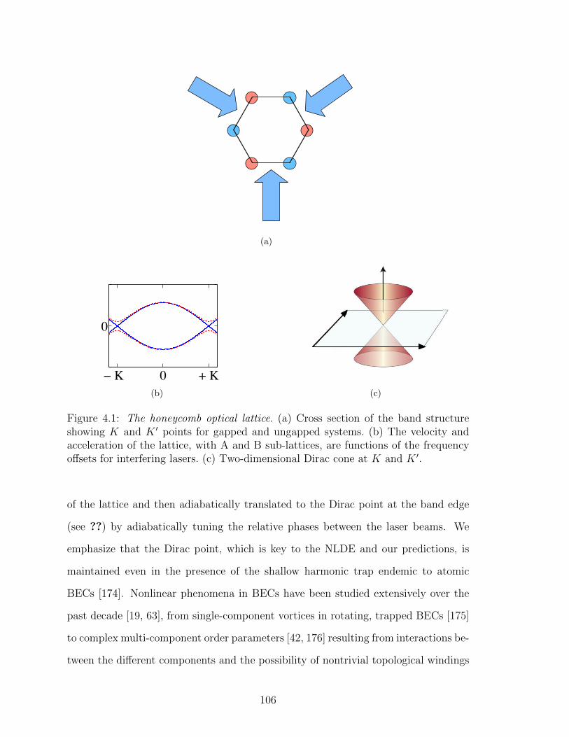
(a)

− K 0 + K

0

(b)

(c)

Figure 4.1: The honeycomb optical lattice. (a) Cross section of the band structureshowing K and K ′ points for gapped and ungapped systems. (b) The velocity andacceleration of the lattice, with A and B sub-lattices, are functions of the frequencyoffsets for interfering lasers. (c) Two-dimensional Dirac cone at K and K ′.

of the lattice and then adiabatically translated to the Dirac point at the band edge

(see ??) by adiabatically tuning the relative phases between the laser beams. We

emphasize that the Dirac point, which is key to the NLDE and our predictions, is

maintained even in the presence of the shallow harmonic trap endemic to atomic

BECs [174]. Nonlinear phenomena in BECs have been studied extensively over the

past decade [19, 63], from single-component vortices in rotating, trapped BECs [175]

to complex multi-component order parameters [42, 176] resulting from interactions be-

tween the different components and the possibility of nontrivial topological windings

106

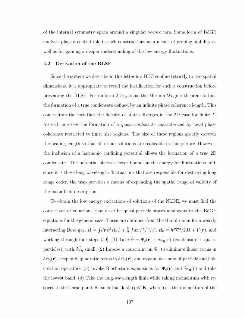
of the internal symmetry space around a singular vortex core. Some form of BdGE

analysis plays a central role in such constructions as a means of probing stability as

well as for gaining a deeper understanding of the low-energy fluctuations.

4.2 Derivation of the RLSE

Since the system we describe in this letter is a BEC confined strictly to two spatial

dimensions, it is appropriate to recall the justification for such a construction before

presenting the RLSE. For uniform 2D systems the Mermin-Wagner theorem forbids

the formation of a true condensate defined by an infinite phase coherence length. This

comes from the fact that the density of states diverges in the 2D case for finite T .

Instead, one sees the formation of a quasi-condensate characterized by local phase

coherence restricted to finite size regions. The size of these regions greatly exceeds

the healing length so that all of our solutions are realizable in this picture. However,

the inclusion of a harmonic confining potential allows the formation of a true 2D

condensate. The potential places a lower bound on the energy for fluctuations and,

since it is these long wavelength fluctuations that are responsible for destroying long

range order, the trap provides a means of expanding the spatial range of validity of

the mean field description.

To obtain the low energy excitations of solutions of the NLDE, we must find the

correct set of equations that describe quasi-particle states analogous to the BdGE

equations for the general case. These are obtained from the Hamiltonian for a weakly

interacting Bose gas, H =∫dr ψ†H0ψ + U

2

∫dr ψ†ψ†ψψ, H0 ≡ ~2∇2/2M + V (r), and

working through four steps [59]. (1) Take ψ = Ψc(r) + δψq(r) (condensate + quasi-

particles), with δψq small. (2) Impose a constraint on Ψc to eliminate linear terms in

δψq(r), keep only quadratic terms in δψq(r), and expand as a sum of particle and hole

creation operators. (3) Invoke Bloch-state expansions for Ψc(r) and δψq(r) and take

the lowest band. (4) Take the long-wavelength limit while taking momentum with re-

spect to the Dirac point K, such that k q K, where q is the momentum of the

107

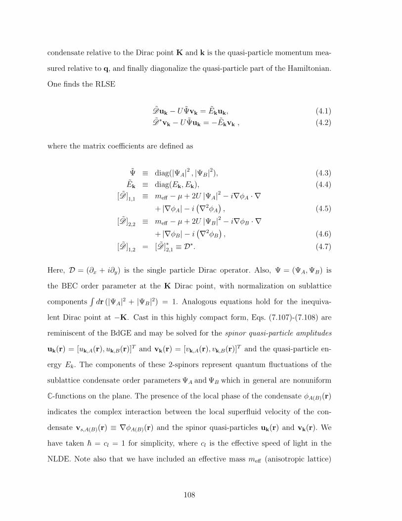
condensate relative to the Dirac point K and k is the quasi-particle momentum mea-

sured relative to q, and finally diagonalize the quasi-particle part of the Hamiltonian.

One finds the RLSE

Duk − UΨvk = Ekuk, (4.1)

D∗vk − UΨuk = −Ekvk , (4.2)

where the matrix coefficients are defined as

Ψ ≡ diag(|ΨA|2 , |ΨB|2), (4.3)

Ek ≡ diag(Ek, Ek), (4.4)

[D ]1,1 ≡ meff − µ+ 2U |ΨA|2 − i∇φA · ∇+ |∇φA| − i

(∇2φA

), (4.5)

[D ]2,2 ≡ meff − µ+ 2U |ΨB|2 − i∇φB · ∇+ |∇φB| − i

(∇2φB

), (4.6)

[D ]1,2 = [D ]∗2,1 ≡ D∗. (4.7)

Here, D = (∂x + i∂y) is the single particle Dirac operator. Also, Ψ = (ΨA,ΨB) is

the BEC order parameter at the K Dirac point, with normalization on sublattice

components∫dr (|ΨA|2 + |ΨB|2) = 1. Analogous equations hold for the inequiva-

lent Dirac point at −K. Cast in this highly compact form, Eqs. (7.107)-(7.108) are

reminiscent of the BdGE and may be solved for the spinor quasi-particle amplitudes

uk(r) = [uk,A(r), uk,B(r)]T and vk(r) = [vk,A(r), vk,B(r)]T and the quasi-particle en-

ergy Ek. The components of these 2-spinors represent quantum fluctuations of the

sublattice condensate order parameters ΨA and ΨB which in general are nonuniform

C-functions on the plane. The presence of the local phase of the condensate φA(B)(r)

indicates the complex interaction between the local superfluid velocity of the con-

densate vs,A(B)(r) ≡ ∇φA(B)(r) and the spinor quasi-particles uk(r) and vk(r). We

have taken ~ = cl = 1 for simplicity, where cl is the effective speed of light in the

NLDE. Note also that we have included an effective mass meff (anisotropic lattice)

108

that competes with the chemical potential µ.

It is important to note that for a moving condensate, the negative-energy modes

cannot be removed and are crucial indicators of Cherenkov radiation. However, in

our case, the Dirac Hamiltonian is not positive-definite since our theory is defined

at zero lattice energy, not the lowest energy Bloch state, so we must respect the

presence of both energy raising and lowering modes. Another important feature is

that the RLSE are reducible to the BdGE when the local lattice potential energy

is the main contributor to the condensate chemical potential and the condensate is

slowly varying (quasi-uniform background), i.e., |µ| >> U , Ej → |µ| ≈ |Σ0|, where

Σ0 = Σ0A(B) ≡ −∫drw∗A(B)H0wA(B) is the local self energy for an arbitrary lattice

site, with wA(B) = w(r− rA(B)) the Wannier functions.

4.3 Physical Parameters and Regimes

We list first the fundamental dimensionful parameters that we use. They are as

follows: the average particle density n0, the chemical potential µ, the lattice spac-

ing a, the s-wave scattering length as, the mass of the constituent bosons M , and

the lattice well depth V0. Several relevant composite quantities may be constructed

from these. These are the effective speed of light cl = tha√

3/2~, the sound speed

cs =√Un0/M , the interaction strength U = 4π~2as/M , the healing length ξ =

tha√

3/2~n0U , and the hopping energy th =∫d2r w∗H0w, where th depends on a and

V0, respectively, through the overlap of Wannier functions and the lattice potential in-

side H0. Two fundamentally important constraints regarding these quantities should

be stated. First, in order to avoid reaching the Landau velocity at the band edge and

creating unwanted excitations we require cl < cs, where cs is the sound speed. Thus

we require tha√

3/2~ <√Un0/M or (tha

√3/2~)(4π~2as n0/M)−1/2 < 1. For 87Rb

with th = ~× 103 Hz , a = 0.5× 10−7 m , as = 5× 10−9 m , n0 = 2× 1012 cm−3, we get

cl/cs . 0.17. Second, in order for our long-wavelength approximation to be correct,

we require the NLDE healing length ξ ≡ tha√

3/2~n0U a; using the same values

109

for the physical parameters, we find ξ ≈ 9.43 a.

Next, we discuss the physical regimes for our theory. In this discussion we take

n0U/th 1. At length scales much larger than the healing length, ξk 1 where k

is a characteristic quasi-particle momentum, excitations are comprised of correlated

particle-hole pairs that propagate with a dispersion given by E ∝ k1/2. This is a Bose

gas of composite particles in the sense that excitations of opposite spin are paired up

(albeit non-locally) to form bosons. In contrast, for ξk 1, excitations are particle-

like which corresponds to the case where spin eigenstates are excited independently.

These states reflect the bipartite structure of the lattice, multi-component with a

Dirac-like dispersion ∝ k, but are local objects and so also reflect the bosonic nature

of the fundamental constituent particles. In this sense, they form a hybrid Dirac-Bose

gas.

4.4 Uniformly Moving Condensate

Now we return to the RLSE and solve them for the simplest case of a uniform

background Ψ(r) ≡ √n0 eiq·r(1, C0)T , where C0 ∈ C contains a relative phase, n0

is the average particle density, and q is the condensate momentum measured with

respect to the Dirac point. In order to obtain the coherence factors and quasi-particle

dispersion, we must then solve a 4 × 4 eigenvalue problem; the RLSE yield: Ek =

c′l~q · k±√

(cl~k)2 + n0Ucl~k. In keeping with the usual Bogoliubov notation found

in the literature, we may write Ek = (c′l/cl) q · ~ε 0k ± E0

k where ~ε 0k ≡ cl~k is the single

quasi-particle energy for zero interaction and E0k =

√(ε0k)

2 + n0Uε 0k is the quasi-

particle energy for a static background. The associated coherence factors can then

be written as |uk,A(B)| = (E0k + cl~k)/

√4E0

kcl~k, |vk,A(B)| = |uk,A(B)|(+ → −). The

full interacting Hamiltonian is given by HRLSE = 14Un2

0A + cl~q −∑′

k(2ε0k + n0U) +∑′

k Ekc†kck , where A is the area of the plane. The first three terms are the mean-

field and quantum corrections to the condensate energy and the last accounts for

the number of quasi-particles present in the system. The constant c′l is defined in

110

terms of the overlap integral between Wannier states at neighboring lattice sites by

c′l =√

3aτ/2~, where τA,B ≡ −∫drw∗A∇wB and τ = |τA,B| 6.

The low energy behavior of the uniform condensate has a rich structure. The

q = 0 case corresponds to a condensate with zero crystal momentum measured from

the Dirac point but with momentum K relative to the lowest Bloch state of the crys-

tal. The idea of a condensate in motion relative to its background has been treated

in both free-space as well as the case of a moving background lattice [64, 70]. Phys-

ically, the lattice potential is moving relative to the stationary condensate (labora-

tory frame). Two-body collisions reduce the momentum of some particles relative

to the lattice (slowing down) and increase the momentum of others (speeding up)

corresponding to a finite depletion of the condensate. In the laboratory frame, a two-

particle collision appears as one particle gaining a component of momentum to the

left and the other a component to the right. This is consistent with the well known

particle-hole symmetry of the Dirac Hamiltonian: negative energy states can be inter-

preted as positive energy states that propagate in the opposite direction. In our theory

these are quasi-particles with momentum K − k (for the K-Dirac point) relative to

the lowest Bloch state.

For q=0 then, we get E(±)k ≡±E0

k = ±√

(ε0k)2 + n0Uε0k. The two energy regimes

evident here are separated by the condition cl~k/n0U ≡ ξk ≈ 1. At short wave-

length, kξ 1 so that E(±)k ≈ ±(cl~k + n0U/2), where the dominant first term

reflects only the presence of the honeycomb lattice, while the second term is a small

mean-field Hartree shift due to the interaction with the background. When kξ 1,

we find E(±)k ≈ ±

√k/ξ. These are collective excitations induced by the particle in-

teractions just above the condensate energy. The presence of negative energy modes

means that the condensate may lower its energy through spontaneous emission of

radiation. This process can be suppressed by introducing an anisotropy in the lat-

6Note that whereas for the effective speed of light we have [cl] = m·s−1, in contrast [c′l] = m2 ·s−1since τA,B is an integral over the gradient operator rather than the Laplacian.

111

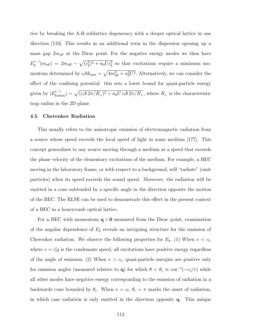
tice by breaking the A-B sublattice degeneracy with a deeper optical lattice in one

direction [133]. This results in an additional term in the dispersion opening up a

mass gap 2meff at the Dirac point. For the negative energy modes we then have

E(−)k (meff) = 2meff −

√(ε0k)

2 + n0Uε0k so that excitations require a minimum mo-

mentum determined by cl~kmin =√

4m2eff + n2

0U2. Alternatively, we can consider the

effect of the confining potential: this sets a lower bound for quasi-particle energy

given by |E(−)k(min)| ∼

√(cl~ 2π/R⊥)2 + n0U cl~ 2π/R⊥, where R⊥ is the characteristic

trap radius in the 2D plane.

4.5 Cherenkov Radiation

This usually refers to the anisotropic emission of electromagnetic radiation from

a source whose speed exceeds the local speed of light in some medium [177]. This

concept generalizes to any source moving through a medium at a speed that exceeds

the phase velocity of the elementary excitations of the medium. For example, a BEC

moving in the laboratory frame, or with respect to a background, will “radiate” (emit

particles) when its speed exceeds the sound speed. Moreover, the radiation will be

emitted in a cone subtended by a specific angle in the direction opposite the motion

of the BEC. The RLSE can be used to demonstrate this effect in the present context

of a BEC in a honeycomb optical lattice.

For a BEC with momentum q> 0 measured from the Dirac point, examination

of the angular dependence of Ek reveals an intriguing structure for the emission of

Cherenkov radiation. We observe the following properties for Ek. (1) When v < cl,

where v = c′lq is the condensate speed, all excitations have positive energy regardless

of the angle of emission. (2) When v > cl, quasi-particle energies are positive only

for emission angles (measured relative to q) for which θ < θc ≡ cos−1(−cl/v) while

all other modes have negative energy corresponding to the emission of radiation in a

backwards cone bounded by θc. When v = cl, θc = π marks the onset of radiation,

in which case radiation is only emitted in the direction opposite q. This unique

112

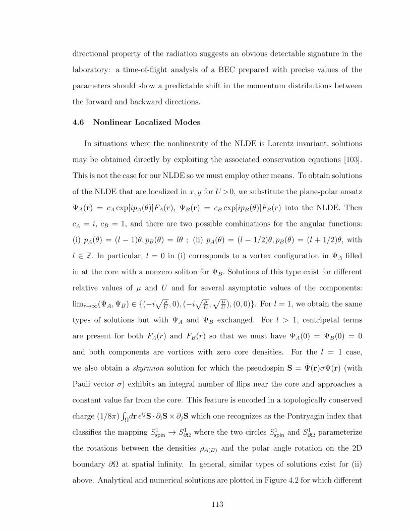
directional property of the radiation suggests an obvious detectable signature in the

laboratory: a time-of-flight analysis of a BEC prepared with precise values of the

parameters should show a predictable shift in the momentum distributions between

the forward and backward directions.

4.6 Nonlinear Localized Modes

In situations where the nonlinearity of the NLDE is Lorentz invariant, solutions

may be obtained directly by exploiting the associated conservation equations [103].

This is not the case for our NLDE so we must employ other means. To obtain solutions

of the NLDE that are localized in x, y for U >0, we substitute the plane-polar ansatz

ΨA(r) = cA exp[ipA(θ)]FA(r), ΨB(r) = cB exp[ipB(θ)]FB(r) into the NLDE. Then

cA = i, cB = 1, and there are two possible combinations for the angular functions:

(i) pA(θ) = (l − 1)θ, pB(θ) = lθ ; (ii) pA(θ) = (l − 1/2)θ, pB(θ) = (l + 1/2)θ, with

l ∈ Z. In particular, l = 0 in (i) corresponds to a vortex configuration in ΨA filled

in at the core with a nonzero soliton for ΨB. Solutions of this type exist for different

relative values of µ and U and for several asymptotic values of the components:

limr→∞(ΨA,ΨB) ∈ (−i√

µU, 0), (−i

√µU,√

µU

), (0, 0). For l = 1, we obtain the same

types of solutions but with ΨA and ΨB exchanged. For l > 1, centripetal terms

are present for both FA(r) and FB(r) so that we must have ΨA(0) = ΨB(0) = 0

and both components are vortices with zero core densities. For the l = 1 case,

we also obtain a skyrmion solution for which the pseudospin S = Ψ(r)σΨ(r) (with

Pauli vector σ) exhibits an integral number of flips near the core and approaches a

constant value far from the core. This feature is encoded in a topologically conserved

charge (1/8π)∫

Ωdr εijS · ∂iS× ∂jS which one recognizes as the Pontryagin index that

classifies the mapping S1spin → S1

∂Ω where the two circles S1spin and S1

∂Ω parameterize

the rotations between the densities ρA(B) and the polar angle rotation on the 2D

boundary ∂Ω at spatial infinity. In general, similar types of solutions exist for (ii)

above. Analytical and numerical solutions are plotted in Figure 4.2 for which different

113

0

0.5

1

|ψA

| , |ψ

B|

(a) (b)

0

0.5

1

|ψA

| , |ψ

B|

(c) (d)

0 50

0.5

1

|ψA

| , |ψ

B|

0 5

(e) r/ξ (f) r/ξ

Figure 4.2: Localized solutions of the NLDE. ΨA (red dashed curves) and ΨB

(blue solid curves), in units of NLDE healing length ξ: (a) vortex/soliton, (b) ring-vortex/soliton, (c) half-quantum vortex, (d) planar skyrmion, (e) line skyrmion,and (f) line-soliton.

114

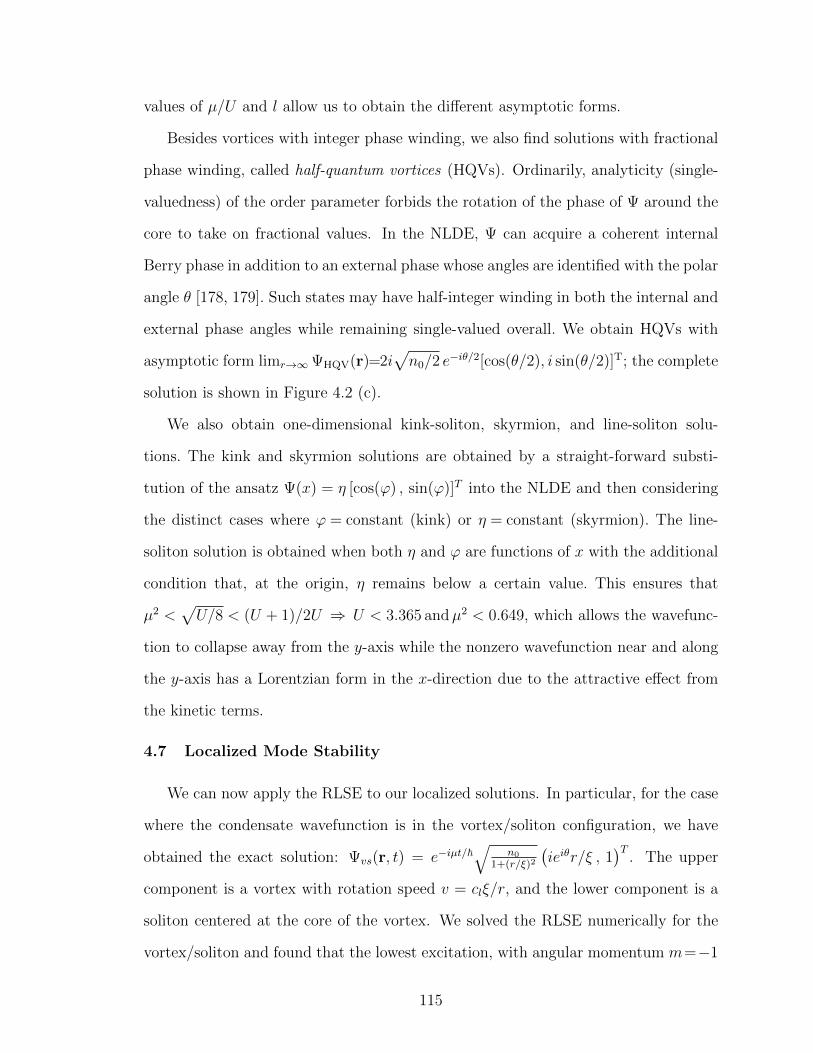
values of µ/U and l allow us to obtain the different asymptotic forms.

Besides vortices with integer phase winding, we also find solutions with fractional

phase winding, called half-quantum vortices (HQVs). Ordinarily, analyticity (single-

valuedness) of the order parameter forbids the rotation of the phase of Ψ around the

core to take on fractional values. In the NLDE, Ψ can acquire a coherent internal

Berry phase in addition to an external phase whose angles are identified with the polar

angle θ [178, 179]. Such states may have half-integer winding in both the internal and

external phase angles while remaining single-valued overall. We obtain HQVs with

asymptotic form limr→∞ΨHQV(r)=2i√n0/2 e

−iθ/2[cos(θ/2), i sin(θ/2)]T; the complete

solution is shown in Figure 4.2 (c).

We also obtain one-dimensional kink-soliton, skyrmion, and line-soliton solu-

tions. The kink and skyrmion solutions are obtained by a straight-forward substi-

tution of the ansatz Ψ(x) = η [cos(ϕ) , sin(ϕ)]T into the NLDE and then considering

the distinct cases where ϕ = constant (kink) or η = constant (skyrmion). The line-

soliton solution is obtained when both η and ϕ are functions of x with the additional

condition that, at the origin, η remains below a certain value. This ensures that

µ2 <√U/8 < (U + 1)/2U ⇒ U < 3.365 andµ2 < 0.649, which allows the wavefunc-

tion to collapse away from the y-axis while the nonzero wavefunction near and along

the y-axis has a Lorentzian form in the x-direction due to the attractive effect from

the kinetic terms.

4.7 Localized Mode Stability

We can now apply the RLSE to our localized solutions. In particular, for the case

where the condensate wavefunction is in the vortex/soliton configuration, we have

obtained the exact solution: Ψvs(r, t) = e−iµt/~√

n0

1+(r/ξ)2

(ieiθr/ξ , 1

)T. The upper

component is a vortex with rotation speed v = clξ/r, and the lower component is a

soliton centered at the core of the vortex. We solved the RLSE numerically for the

vortex/soliton and found that the lowest excitation, with angular momentum m=−1

115

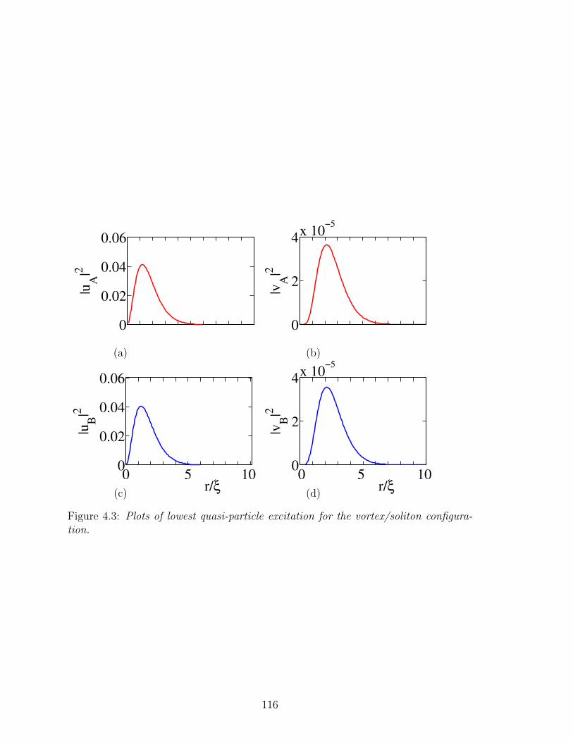
0

0.02

0.04

0.06

|uA

|2

0

2

4x 10

−5

|vA

|2

(a) (b)

0 5 10 0

0.02

0.04

0.06

r/ξ

|uB

|2

0 5 10 0

2

4x 10

−5

r/ξ

|vB

|2

(c) (d)

Figure 4.3: Plots of lowest quasi-particle excitation for the vortex/soliton configura-tion.

116

(relative to the condensate), has the eigenenergy E−1 =−3.9274 + 0.0020 i, in units

of n0U . This excitation, having angular momentum equal in magnitude but opposite

to the vortex rotation, perturbs the vortex by adding a component of the state that

has zero rotation, effectively driving the vortex energy towards the Dirac point. The

corresponding coherence factors are shown in Figure 4.3. They peak in the region

ξ ≤ r ≤ 2ξ with |uA(B),−1|2 ∼ 10−2 and |vA(B),−1|2∼10−5 so that uA(B),−1 >> vA(B),−1,

which results in a positive normalization integral∫d2r (|u−1|2−|v−1|2). This combi-

nation of positive norm and negative energy signals the presence of the anomalous

mode which also occurs for vortices in single-component trapped BECs [180]. To the

left of the peaks, near the core where 0 < r < ξ, excitations are particle-like. There,

the tangential rotation speed of the vortex exceeds the critical velocity for emission

of Cherenkov radiation so that, in the presence of a mechanism for dissipation, par-

ticles are freely radiated out of the condensate. In contrast, for r ≈ 5ξ, we find that

|u−1| ≈ |v−1| so that excitations are roughly equal admixtures of particles and holes

and no radiation is expected.

The anomalous mode has a direct physical interpretation in terms of the preces-

sion of the vortex around the central core. To see this, we first compute the density

fluctuation in the anomalous mode:

δnvs,−1 =∣∣∣〈ψ〉∣∣∣2−|Ψvs|2

=(uT−1Ψ∗vs −ΨT

vsv−1

)e−iE−1t/~ +

(ΨTvsu∗−1 − vT∗−1Ψ∗vs

)eiE−1t/~ . (4.8)

Substituting the expressions for Ψvs, u−1 and v−1 into Eq. (4.8) allows us to obtain

the density fluctuations for the individual components of the condensate. For the

upper component (vortex), we obtain

δnvs,A,−1 = fA(r) e−i(θ−|ReE−1|t/~) eImE−1t/~ + gA(r) ei(θ−|ReE−1|t/~) e−ImE−1t/~ , (4.9)

117

with the radial functions given by fA(r) = n1/20 uA,−1(r) (r/ξ)/

√1 + (r/ξ)2 and gA(r) =

n1/20 vA,−1(r) (r/ξ)/

√1 + (r/ξ)2. Fluctuations are strongest near r ≈ 1.5 ξ with the

main contribution coming from the first term in Eq. (4.9), which describes parti-

cle excitations with only a minimal hole component. For the fluctuations of the

lower component of the condensate (soliton), we obtain an expression similar to

Eq. (4.9) but with the radial functions given by fB(r) = n1/20 uB,−1(r)/

√1 + (r/ξ)2

and gB(r) = n1/20 vB,−1(r)/

√1 + (r/ξ)2. The fluctuations of the soliton contain non-

zero angular terms which is a consequence of the coupling between the vortex and

soliton through the Dirac kinetic terms; in time, through quantum fluctuations, the

soliton will develop a finite rotation. The first term in Eq. (4.9) grows exponentially

and is proportional to exp[i (|ReE−1| t/~− θ )]×exp( ImE−1t/~). The complex factor

describes the precession of the density fluctuation in the anti-clockwise direction. The

additional factor that grows in time does not appear in the analog case for a vortex

in the Gross-Pitaevskii formalism and arises here from the coupling of the spinor

components through the derivative terms in the Dirac Hamiltonian.

We can use Eq. (4.8) to estimate the finite lifetime of the vortex due to this effect.

By requiring that the total number of particles be conserved, we compute the value:

τ = ~ ln2/(2 ImE−1) ≈ 1.88s. We note that this value does not take into account

interactions between the vortex and thermal cloud at finite temperature which would

further reduce the value of τ . Thus, we expect the lifetime for Dirac vortices to be

shorter than vortices in condensates which are stationary with respect to the lattice.

This is expected since the lattice provides a source of friction (dissipation) and bosons

are free to drop to lower energy states. This is of course not the case for fermions

in graphene, for example, due to the presence of the Fermi level which coincides

with the Dirac point. For several of our solutions, we find that the characteristic time

associated with this instability is experimentally reasonable. The lowest quasi-particle

energies for the other localized solutions are: −3.9276 + 0.0019 i; 2.634× 102 + 9.96×

118

104i; −3.9274 + 0.0019 i; 7.8409× 10−3− 9.9993× 102 i; 7.9349× 10−3− 9.9993× 102 i;

for the ring-vortex/soliton, half-quantum vortex, planar skyrmion, line-skyrmion, and

line-soliton respectively, where all quantities are given in units of n0U .

4.8 Conclusion

In conclusion, we have shown that an effective quasi-relativistic system with a

Dirac-like structure may be designed using ordinary cold bosonic atoms as the un-

derlying degrees of freedom. We solved the resulting NLDE for different classes of

nonlinear modes including half-quantum vortices. We derived and solved relativistic

linear stability equations and gave explicit criteria for experimental observation of

Cherenkov radiation, as well as predicting an anomalous mode for the vortex/soliton

solution. Density profiles may be observed by time-of-flight techniques to detect both

massive and massless Dirac fermions in the laboratory [15, 133]; nonlinear modes

involving phase winding can be created by techniques analogous to those used at

JILA [181]; and we anticipate that Bragg scattering can be used to populate the

Dirac cones at both K and K′ points, leading to arbitrary superpositions over our

localized solution types between the two cones, and thereby populating all four com-

ponents of the Dirac spinor.

119

Acknowledgments

We thank Ken O’Hara, Jeff Steinhauer, and Michael Wall for useful discus-

sions. This work was supported by the NSF and the Aspen Center for Physics.

120

CHAPTER 5

ESTABLISHING THE RELATIVISTIC LINEAR STABILITY EQUATIONS:

MICROSCOPIC LATTICE DERIVATION, TRANSITION OF OPERATORS

FROM LATTICE TO CONTINUUM, PROPERTIES OF SPINOR COHERENCE

FACTORS AND INTERACTING GROUND STATE

5.1 Introduction

In this chapter, we provide the complete analysis for the low-energy structure

of BECs in honeycomb lattices to support and build on the material presented in

Chapter 4. This includes a review of the standard Bogoliubov theory for unconfined

BECs with arbitrary spatial profiles, and the complete derivation of the RLSE which

relies heavily on the use of Wannier functions combined with geometry to prove all of

our results, for each step at the microscopic level. We apply the RLSE to a uniform

condensate, for which we provide detailed calculations to obtain the terms describing

interactions of the quasi-particles with the phase of the condensate. This last step

allows us to obtain the prediction of Cherenkov radiation as we have presented in

Chapter 4.

5.2 Standard Theory for a Free Condensate

In this section we reproduce the standard derivation for a nonuniform condensate

as presented in the original article by A. L. Fetter in Ref. [66]. Beginning with

the many-body Hamiltonian for interacting bosons, we first perform the Bogoliubov

transformation, and then specialize the potential to include the lattice; compute the

interacting system first, then turn on the lattice rather than the other way around.

We start again with the Hamiltonian

121

H =

∫d2rψ†H0ψ +

g

2

∫d2rψ†ψ†ψψ , (5.1)

where, H0 ≡ − ~2

2m∇2 + V (~r) , (5.2)

and, V (~r) is the lattice potential and g is the contact interaction coupling strength.

In what follows we proceed in the same manner as in Fetter’s seminal 1972 paper. As

before , we decompose the wavefunction as the sum

ψ(~r) = ζ(~r) a0 + φ(~r), (5.3)

where we have separated out an operator component to the condensate part that

satisfies the bosonic commutation relation:

[a0 , a†0] = 1 . (5.4)

It is clear that the first term on the right hand side of Eq.(5.3) describes the condensate

since it destroys a particle in the mean field ζ which, by itself, is a good approximation

to ψ. The second term destroys a particle in a number of single-particle basis states

of the noninteracting system and describes the part of ψ that deviates from the mean

field. In the Bogoliubov limit a0 → N1/20 but we compute the commutator before

taking this limit to retain the effect of the presence of a macroscopic condensate

field. We can obtain the commutation relations for φ and φ† by starting with the

commutator for ψ and ψ† and using Eqs. (5.3) and (5.4). Starting from

[ψ(~r), ψ†(~r ′)

]= δ(~r − ~r ′) , (5.5)[

ψ(~r), ψ(~r ′)]

= 0 , (5.6)[ψ†(~r), ψ†(~r ′)

]= 0 . (5.7)

We then have

122

[ψ(~r), ψ†(~r ′)

]=

[ζ(~r) a0 + φ(~r) , ζ∗(~r ′) a†0 + φ†(~r ′)

](5.8)

= ζ(~r) ζ∗(~r ′)[a0 , a

†0

]+ ζ(~r)

[a0 , φ

†(~r ′)]

+ ζ∗(~r ′)[φ(~r) , a†0

]+[φ(~r) , φ†(~r ′)

](5.9)

⇒[φ(~r) , φ†(~r ′)

]= δ(~r − ~r ′) − ζ(~r) ζ∗(~r ′) , (5.10)

where we have used Eq. (5.4) and

[a0 , φ

†(~r ′)]

=[φ(~r) , a†0

]= 0 . (5.11)

Also,

[ψ(~r), ψ(~r ′)

]=

[ζ(~r) a0 + φ(~r) , ζ(~r ′) a0 + φ(~r ′)

](5.12)

= ζ(~r) ζ(~r ′) [a0 , a0] + ζ(~r)[a0 , φ(~r ′)

]+ ζ(~r ′)

[φ(~r) , a0

]+[φ(~r) , φ(~r ′)

](5.13)

⇒[φ(~r) , φ(~r ′)

]= 0 . (5.14)

Similarly,

[ψ†(~r), ψ†(~r ′)

]=

[ζ∗(~r) a†0 + φ†(~r) , ζ∗(~r ′) a†0 + φ†(~r ′)

](5.15)

= ζ∗(~r) ζ∗(~r ′)[a†0 , a

†0

]+ ζ∗(~r)

[a†0 , φ

†(~r ′)]

+ ζ∗(~r ′)[φ†(~r) , a†0

]+[φ†(~r) , φ†(~r ′)

](5.16)

⇒[φ†(~r) , φ†(~r ′)

]= 0 . (5.17)

In the Bogoliubov limit the condensate wavefunction has no operator part and ψ may

be written as

123

ψ(~r) = Ψ(~r) + φ(~r) , (5.18)

where the condensate wavefunction has well defined phase and particle density and

so may be written as

Ψ(~r) =

√N0

AeiS(~r)

√ρ(~r) . (5.19)

Here A is the area of the planar system. The radial part is normalized as

A−1

∫d2rρ(~r) = 1. (5.20)

With these definitions the usual bosonic commutation relations become

[φ(~r), φ†(~r ′)

]= eiS(~r) e−iS(~r ′) δ(~r, ~r ′), (5.21)

where, δ(~r, ~r ′) = δ(~r − ~r ′) − A−1√ρ(~r)

√ρ(~r ′) . (5.22)

As before, we transform to the new Hamiltonian

K = H − µN = H − µ

∫d2r ψ† ψ . (5.23)

Now, inserting Eq. (5.3) into Eq. (5.23), expanding through second order in the

operator part and eliminating the linear terms by forcing the condensate wavefunction

to obey the equation

[H0 − µ + g |Ψ|2

]Ψ = 0. (5.24)

These steps are the same as before but now for a single component wavefunction. We

arrive at the Bogoliubov Hamiltonian K = K0 + K2 where

124

K0 =

∫d2r Ψ∗(~r)

[H0 − µ +

g

2|Ψ(~r)|2

]Ψ(~r)

and , K2 =

∫d2r φ†(~r)

[H0 − µ + 2g |Ψ(~r)|2

]φ(~r)

+g

2

∫d2r

[Ψ∗(~r)]2 φ(~r) φ(~r) + φ†(~r) φ†(~r) [Ψ(~r)]2

, (5.25)

where in addition to the kinetic operator we also have an arbitrary external potential

in the first two terms. Eq.(5.25) is quadratic in the field operators and so may be

diagonalized with the appropriate field redefinition. Next, we diagonalize Eq.(5.25)

with the linear transformation

φ(~r) = eiS(~r)

′∑j

[uj(~r) αj − v∗j (~r) α

†j

], (5.26)

φ†(~r) = e−iS(~r)

′∑j

[u∗j(~r) α

†j − vj(~r) αj

]. (5.27)

The prime on the summation sign indicates that we are omitting the condensate from

the sum. The αj’s and α†j’s inherit standard bosonic commutation relations from φ

and φ† and the transformation coefficients obey the completeness relations

′∑j

[uj(~r) u

∗j(~r

′) − v∗j (~r) vj(~r′)]

= δ(~r, ~r ′) (5.28)

′∑j

[uj(~r) v

∗j (~r

′) − v∗j (~r) uj(~r′)]

= 0 (5.29)

′∑j

[u∗j(~r) vj(~r

′) − vj(~r) u∗j(~r

′)]

= 0 . (5.30)

Substituting Eqs. (5.26) and (5.27) into Eq. (5.25) and, after some tedious algebra

as we have previously shown, we arrive at

125

K =

∫d2r Ψ∗(~r)

[H0 − µ +

g

2|Ψ(~r)|2

]Ψ(~r)

+′∑

j,k

∫d2r

αjα

†k

[vjLv∗k −

1

2g |Ψ|2 (ujv

∗k + u∗kvj)

]+ α†jαk

[u∗jLuk −

1

2g |Ψ|2 (v∗juk + vku

∗j)

]− αjαk

[vjLuk −

1

2g |Ψ|2 (ujuk + ujvk)

]− α†jα

†k

[ujLvk −

1

2g |Ψ|2 (u∗ju

∗k + v∗j v

∗k)

], (5.31)

where we have used the condensed notation

L = − ~2

2m[∇ + i ∇S(~r)]2 + V (~r) − µ + 2g |Ψ(~r)|2 . (5.32)

The next step determines the functional form of the transformation coefficients and

further simplifies the Hamiltonian as we continue to work towards diagonalization.

Assume the following coupled eigenvalue equations as constraints

L uj − g |Ψ|2 vj = Ejuj (5.33)

L∗ vj − g |Ψ|2 uj = − Ejvj , (5.34)

so that Eq.(5.31) reduces to

K =

∫d2r Ψ∗(~r)

[H0 − µ +

g

2|Ψ(~r)|2

]Ψ(~r)

+1

2

′∑j,k

∫d2r[(Ej + Ek)(α

†jαku

∗juk − αjα

†kvjv

∗k)

+ (Ej − Ek)(αjαkukvj − α†jα†ku∗jv∗k)]. (5.35)

Multiplying Eq. (5.33) by u∗k and Eq. (5.34) by v∗k and integrating, we get

(Ej − E∗k)

∫d2r(u∗juk − v∗j vk) = 0 , (5.36)

126

which further leads to

∫d2r[u∗j(~r)uk(~r) − v∗j (~r)vk(~r)

]= δj,k . (5.37)

Similarly, multiplying by vk and uk and integrating gives

∫d2r [uj(~r)vk(~r) − uk(~r)vj(~r)] = 0 . (5.38)

Using the results of Eqs.(5.36) - (5.38) , the final diagonal form of the Hamiltonian

is

K =

∫d2r Ψ∗(~r)

[H0 − µ +

g

2|Ψ(~r)|2

]Ψ(~r)

−′∑

j

Ej

∫d2r |vj(~r)|2 +

′∑j

Ejα†jαj . (5.39)

5.3 Bogoliubov Theory for a Condensate at Dirac Point of a HoneycombLattice

So far, what we have presented is simply a review of the main points in the Bogoli-

ubov transformation for a nonuniform Bose gas [66]. Our notation is slightly different

in that we have kept H0 in our equations to allow for a more general single-particle

Hamiltonian which includes an arbitrary external potential. For our particular in-

terest, we would like to know how the structure of the transformation changes as

the lattice strength is turned up from zero to the tight-binding limit. Namely, what

do Eqs.(5.33), (5.34) and (5.39) map to in the presence of a strong, two-dimensional

lattice potential?

In going from the case where the lattice potential is turned off, we can imagine

adiabatically tuning V (~r) so that the order parameter (the average field of the many-

body system) gradually settles into a solution that is well described by a set of Bloch

states. Since Bloch states form a complete orthonormal set there is certainly nothing

preventing us from expressing any well behaved function in terms of such a basis but,

127

only as we increase the depth of the potential wells of the lattice do the individual

states, labeled by wave-number ~k, become stationary states of the system. The first

step then is to make the leap to the tight-binding limit and trust that a straightforward

substitution of Bloch states (or linear combinations of them) into the key equations

will determine the correct structure of the theory in the tight-binding limit.

The first assumption is that, in the tight-binding limit, we can further decompose

the condensate and operator parts of the wavefunction in terms of the individual

sublattices. To compute the commutation relations , Eqs. (5.10), (5.11), (5.14), and

(5.17), corresponding to taking the tight-binding limit, the condensate and quasi-

partcle terms in Eq. (5.3) may be expanded as follows:

ζ(~r) = ζA(~r) + ζB(~r) , (5.40)

φ(~r) = φA(~r) + φB(~r) , (5.41)

with,

ζA(~r) ≡∑A

ei~k·(~r−~rA) wAi

(~r − ~rA) , (5.42)

ζB(~r) ≡∑B

ei~k·(~r−~rB) wBi

(~r − ~rB) , (5.43)

φA(~r) ≡∑A

ai ei~k·(~r−~rA) w(~r − ~rA) (5.44)

φB(~r) ≡∑B

bi ei~k·(~r−~rB)w(~r − ~rB) . (5.45)

Equation (5.3) becomes

ψ(~r ) = a0

∑A

ei~k·(~r−~rA)wAi

(~r − ~rA) + b0

∑B

ei~k·(~r−~rB) wBi

(~r − ~rB)

+∑A

ai ei~k·(~r−~rA)w(~r − ~rA) +

∑B

bi ei~k·(~r−~rB) w(~r − ~rB) . (5.46)

This decomposition also assumes that overlap between any two sites is small enough

so that the field operator algebra, that is continuously parameterized by the points on

128

the two-dimensional manifold, breaks up into a discrete set of algebras parameterized

by each lattice site. The wAiand wBi

are localized at the lattice sites Ai and Bi

respectively but the subscripts indicate that these are generally different for each site.

Note the important difference between the condensate and quasi-partcle parts. The

first and second summations on the right hand side of Eq.(5.46) destroy particles in the

single-particle wavefunction described by the sum over modified Bloch states; these

are states with well-defined density and phase for the A and B sublattice condensates.

Because of this, the condensate is really a two-state system. On the other hand, the

third and fourth summations destroy particles at individual lattice sites creating a

many-body superposition of single-particle states. Computing the lattice counterpart

to Eq.(5.10) using Eq.(5.46), we get

[ψ(~r ) , ψ†(~r ′)

]=

[a0, a

†0

]∑A,A′

e−i~k·(~r ′−~rA′ ) w∗A′i(~r

′ − ~rA′) ei~k·(~r−~rA) wAi(~r − ~rA)

+[b0, b

†0

]∑B,B′

e−i~k·(~r ′−~rB′ ) w∗B′i(~r

′ − ~rB′) ei~k·(~r−~rB) wBi(~r − ~rB)

+∑A

[ai , a

†i

]e−i

~k·(~r ′−~rA) w∗(~r ′ − ~rA) ei~k·(~r−~rA) w(~r − ~rA)

+∑B

[bi , b

†i

]e−i

~k·(~r ′−~rB) w∗(~r ′ − ~rB)ei~k·(~r−~rB) w(~r − ~rB) (5.47)

= δ(~r − ~r ′) (5.48)

=⇒ ∑A

[ai , a

†i

]e−i

~k·(~r ′−~rA) w∗(~r ′ − ~rA) ei~k·(~r−~rA) w(~r − ~rA)

+∑B

[bi , b

†i

]e−i

~k·(~r ′−~rB) w∗(~r ′ − ~rB)ei~k·(~r−~rB) w(~r − ~rB)

= δ(~r − ~r ′)

−∑A,A′

e−i~k·(~r ′−~rA′ ) w∗A′i(~r

′ − ~rA′) ei~k·(~r−~rA) wAi(~r − ~rA)

−∑B,B′

e−i~k·(~r ′−~rB′ ) w∗B′i(~r

′ − ~rB′) ei~k·(~r−~rB) wBi(~r − ~rB) . (5.49)

This can be written in condensed notation

129

∑A

[φAi

(~r ), φ†Ai(~r ′ )

]+∑B

[φBi

(~r ), φ†Bi(~r ′ )

]=

δ(~r − ~r ′) −∑A

ζ∗Ai(~r ′) ζAi

(~r) −∑B

ζ∗Bi(~r ′) ζBi

(~r) . (5.50)

The full Hamiltonian for the system is symmetric in the sublattice labels A and B

which allows us to write

∑A

[φAi

(~r ), φ†Ai(~r ′ )

]=

1

2δ(~r − ~r ′) −

∑A

ζ∗Ai(~r ′) ζAi

(~r) , (5.51)

∑B

[φBi

(~r ), φ†Bi(~r ′ )

]=

1

2δ(~r − ~r ′) −

∑B

ζ∗Bi(~r ′) ζBi

(~r) . (5.52)

These are the lattice analogues of Eq.(5.10). Next, we compute the counterpart to

Eq.(5.11). This is straightforward and needs no detailed calculation since our initial

assumption; that the operators for condensate and non-condensate particles commute;

still holds. We obtain

[a0 , φ

†A(~r ′)

]=[φA(~r ) , a†0

]= 0 , (5.53)[

a0 , φ†B(~r ′)

]=[φB(~r ) , a†0

]= 0 , (5.54)[

b0 , φ†A(~r ′)

]=[φA(~r ) , b†0

]= 0 , (5.55)[

b0 , φ†B(~r ′)

]=[φB(~r ) , b†0

]= 0 . (5.56)

Similarly Eq.(5.14) becomes

[φA(~r ) , φA(~r ′)

]= 0 , (5.57)[

φA(~r ) , φB(~r ′)]

= 0 , (5.58)[φB(~r ) , φB(~r ′)

]= 0 . (5.59)

Eq.(5.17) becomes

130

[φ†A(~r ) , φ†A(~r ′)

]= 0 , (5.60)[

φ†A(~r ) , φ†B(~r ′)]

= 0 , (5.61)[φ†B(~r ) , φ†B(~r ′)

]= 0 . (5.62)

Next, we take the Bogoliubov limit in which the condensate part of the wavefunction

becomes a pure complex number by letting a0 , b0 → N1/20 ,

ψ(~r ) = ΨA(~r ) + ΨB(~r ) + φA(~r ) + φB(~r ) , (5.63)

where the condensate wavefunction is defined as

Ψ(~r ) = ΨA(~r ) + ΨB(~r ) , (5.64)

and,

ΨA(~r ) = ζA(~r )N1/20 (5.65)

ΨB(~r ) = ζB(~r )N1/20 . (5.66)

Expressing the condensate in terms of a local particle number and phase,

ΨA(~r ) =∑A

ei~k·(~r−~rA) wAi

(~r − ~rA) =∑A

ei~k·(~r−~rA)√nAi

eiSAi w(~r − ~rA) , (5.67)

ΨB(~r ) =∑B

ei~k·(~r−~rB) wBi

(~r − ~rB) =∑B

ei~k·(~r−~rB)√nBi

eiSBi w(~r − ~rB) , (5.68)

where we assume the local functions normalized as

∫d2r w∗w = 1 , (5.69)

so that

131

∫d2rΨ∗A(~r ) ΨA(~r ) =

∑A

nAi= N0,A , (5.70)∫

d2rΨ∗B(~r ) ΨB(~r ) =∑B

nBi= N0,B , (5.71)

where the total number of condensate particles is defined in terms of the total in each

sublattice

N0 ≡ N0,A + N0,B . (5.72)

Substituting Eq.(5.64) into Eq.(5.24), we get

[H0 − µ + g |ΨA|2 + gΨ∗AΨB + gΨ∗BΨA + g |ΨB|2

](ΨA + ΨB) = 0 . (5.73)

Next, we substitute Eq.(5.67) and (5.68) into Eq.(5.73) and multiply on the left by

e−i~k·(~r−~rAj

) w∗(~r − ~rAj) , (5.74)

and integrate over the plane. Here the subscript Aj indicates that this quantity is

associated with the jth site of the A sublattice. We restrict to the condition of nearest-

neighbor interactions which greatly simplifies the resulting expression since all A-A

and B-B transitions, except for on-site kinetic and potential terms, are eliminated and

the later may be neglected as an overall self-energy. Then, only integrals involving

neighboring A-B sites remain in the sum. Similarly, in the interactions only on-

site terms are non-negligible, i.e., overlap of functions w belonging to the same site.

Eq.(5.73) then reduces to

−th[√

nBjeiSBj ei

~k·(~rAj−~rBj

) +√nBj−n1

eiSBj−n1 e

i~k·(~rAj−~rBj−n1

)

+√nBj−n2

eiSBj−n2 e

i~k·(~rAj−~rBj−n2

)]− µ√nAj

eiSAj + U∣∣∣√nAj

eiSAj

∣∣∣2 √nAjeiSAj

= 0 . (5.75)

132

The hopping integral and interaction energy are respectively,

th = −∫d2r w∗(~r − ~rAj

)H0w(~r − rBj) (5.76)

and ,

U = g

∫d2r w∗j w

∗j wj wj , (5.77)

where Aj and Bj refer to nearest neighbor sites. In terms of the nearest neighbor

vectors ~δ1, ~δ2, and ~δ3, we get

−th[√

nBjeiSBj ei

~k·~δ3 +√nBj−n1

eiSBj−n1 ei

~k·~δ1 +√nBj−n2

eiSBj−n2 ei

~k·~δ2]

−µ√nAjeiSAj + U

∣∣∣√nAjeiSAj

∣∣∣2 √nAjeiSAj = 0. (5.78)

Next we insert particular values for the nearest-neighbor displacement vectors ~δ and

evaluate ~k at the Brillouin zone corner, defined by ~k = ~K = (0, 4π/3) , ~δ1 = ( 12√

3,−1

2),

~δ2 = ( 12√

3, 1

2), ~δ3 = (− 1√

3, 0), to obtain

−th[√

nBkeiSBk e0 +

√nBk−n1

eiSBk−n1 e−i2π/3 +

√nBk−n2

eiSBk−n2 ei2π/3

]−µ√nAk

eiSAk + U∣∣√nAk

eiSAk

∣∣2 √nAkeiSAk = 0 . (5.79)

Reducing the exponentials gives

−th[√

nBkeiSBk +

√nBk−n1

eiSBk−n1 (−1/2− i

√3/2)

+√nBk−n2

eiSBk−n2 (−1/2 + i

√3/2)

]−µ√nAk

eiSAk + U∣∣√nAk

eiSAk

∣∣2 √nAkeiSAk = 0 . (5.80)

Regrouping terms gives us

−th[(√

nBkeiSBk − √nBk−n1

eiSBk−n1

)(1/2 + i

√3/2)

+(√

nBkeiSBk − √nBk−n2

eiSBk−n2

)(1/2− i

√3/2)

]−µ√nAk

eiSAk + U∣∣√nAk

eiSAk

∣∣2 √nAkeiSAk = 0 . (5.81)

133

Dividing through by the lattice spacing, a, and taking the continuum limit, the first

two terms that contain differences become derivatives of the condensate wavefunction

with respect to the lattice translation vectors. Abusing the notation a bit, we redefine

the components of the condensate wavefunction in terms of the density and phase as

ΨA(~r) ≡√ρA(~r) eiSA(~r) , (5.82)

ΨB(~r) ≡√ρB(~r) eiSB(~r) . (5.83)

Here the density and phase are the continuum limits of those in Eq.(5.81). Eq.(5.81)

becomes

−th[∂ΨB

∂n1

(1/2 + i√

3/2) +∂ΨB

∂n2

(1/2− i√

3/2)

]− µΨA + U |ΨA|2 ΨA = 0 .(5.84)

After transforming to x and y coordinates and working through some algebra, we

arrive at

i th a√

3

2 ~(∂x − i∂y) ΨB − U |ΨA|2 ΨA + µΨA = 0 . (5.85)

The same steps lead to a similar equation for ΨB

i th a√

3

2 ~(∂x + i∂y) ΨA − U |ΨB|2 ΨB + µΨB = 0 . (5.86)

Replacing the constant in front of the derivative terms by the speed of sound in the

condensate, we obtain

i ~cl (∂x + i∂y) ΨA − U |ΨB|2 ΨB + µΨB = 0 , (5.87)

i ~cl (∂x − i∂y) ΨB − U |ΨA|2 ΨA + µΨA = 0 . (5.88)

Eqs. (5.87) and (5.88) comprise the nonlinear Dirac equation for one Dirac point.

134

5.3.1 Transition of Operators Between Lattice and Continuum Limits

We should establish a more rigorous connection between operators at the lattice

scale and those that are defined after taking the long-wavelength limit. In particular,

when working with operator terms in the Hamiltonian in the long-wavelength limit

we may wish to diagonalize certain terms inducing off-diagonal terms elsewhere. We

may ask what the relationship is between the operators used to diagonalize before

taking the long-wavelength and those that diagonalize after taking this limit. On the

lattice scale it is clear that an operator that creates a boson on the A sublattice, say,

and one that creates a boson in some superposition of A and B are related by some

sort of spatial rotation while at long distances the transformation must map to some

unitary operation acting on the pseudospin structure of the wavefunction.

On the lattice scale, the operator that creates a boson in the single-particle state

with momentum ~~k, where a is the lattice spacing, is given by

c†~k =∑A,B

< wAi(Bi)|~k > c†~k,Ai(Bi), (5.89)

where, c†~k,Ai(Bi)creates a boson at some site on the lattice and the projection is defined

as

< wAi(Bi)|~k >≡∫d2re i

~k·~r w∗(~r − ~rAi(Bi)) . (5.90)

The summation is defined over the entire lattice. Because of the isotropy of the system

we may consider states with a given magnitude k = |~k| and also, define a†k,i ≡ c†k,Ai

and b†k,i ≡ c†k,Bi. We are being very loose here with the lattice notation as we are using

the single index i to denote a site which is determined by a two-dimensional lattice

vector. With these definitions, the operator that creates a boson with momentum ~ k

on the A sublattice is

135

a†k ≡∑A

< wAi|k > c†k,Ai

, (5.91)

similarly, for the B sublattice, we have

b†k ≡∑B

< wBi|k > c†k,Bi

. (5.92)

Then, at the lattice scale, a unitary operator that creates a superposition state over

A and B must be

q†k = U∗(L)aq a†k + U∗(L)bq b

†k (5.93)

=∑A,B

(U∗(L)aq < k|wAi

> c†k,Ai+ U∗(L)bq < k|wBi

> c†k,Bi

), (5.94)

with |U(L)aq|2 + |U(L)bq|2 = 1 and the subscript (L) indicates that these operator

is defined at the lattice scale. We can connect a pure state to a superposition state

through a spatial rotation. For example, since we have honeycomb lattice symmetry,

a rotation by an integer multiple of π/3 produces

R(nπ/3)ψA(~r ) = R(nπ/3)∑A

w(~r − ~rA) ei~k·(~r− ~rA)

=∑A

[R(nπ/3)w(~r − ~rA)][R(nπ/3)ei

~k·(~r− ~rA)]

=∑B

w(~r − ~rB) ei~k·(~r− ~rB)

= ψB(~r ) , (5.95)

so that,

Rnπ/3 |0, ..., nA,k = 1, ..., 0 >= |0, ..., nB,k = 1, ..., 0 > , (5.96)

where Rnπ/3 is the action of a rotation by nπ/3 on the many body state with a single

boson in a state with momentum ~p = ~~k on sublattice A, i.e.,

136

|0, ..., nA,k = 1, ..., 0 > ≡ a†k |O > . (5.97)

Note also that the induced transformation possesses the involution property

R2nπ/3 |0, ..., nA,k = 1, ..., 0 > = Rnπ/3 |0, ..., nB,k = 1, ..., 0 >

= |0, ..., nA,k = 1, ..., 0 > (5.98)

⇒ R2nπ/3 = 1 . (5.99)

For a mixed operator acting on the ground state we have

q†k |O > = C∗k,aq |0, ..., nA,k = 1, ..., 0 > +C∗k,bq |0, ..., nB,k = 1, ..., 0 >

= C∗k,aq a†k |O > +C∗k,bq Rnπ/3 a

†k |O > (5.100)

⇒ q†k =(C∗k,aq + C∗k,bq Rnπ/3

)a†k (5.101)

=(1 + ei α Rnπ/3

)a†k , (5.102)

where in the last step we have replaced complex constants by a phase difference in the

second term. To define spatial rotations in two-dimensions we require one generator

but since we are rotating complex functions we must also specify a relative phase

rotation by a phase angle δ embedded in the spatial rotation. For an infinitesimal

spatial rotation ε , continuity in the phase of the wavefunction demands that δ must

also be small so that ei δ/2 = 1 + iδ/2 + h.c.. We obtain

(1 + ei α Rε

)≡ e~ε ·

~Q(L) = 1(L) + ε1 Q(L),1 + ε2 Q(L),2 + h.c. (5.103)

where the bold notation indicates the action on the state space induced by the spatial

and phase rotations in the plane. For a spatial plus phase rotation in two-dimensions

we require the matrices

[1 00 1

],

[0 − e i δ/2

e− i δ/2 0

]. (5.104)

137

For small δ we can expand the second matrix

[0 − e i δ/2

e− i δ/2 0

]≈

[0 − (1 + i δ/2)

(1 − i δ/2) 0

](5.105)

≈[

0 − 11 0

]− i δ/2

[0 11 0

]. (5.106)

Extracting a factor of − i we obtain the Pauli matrices that are relevant to the plane.

With the expansion parameter in Eq.(5.103) defined such that ε1 = ε δ/2 and ε2 = ε

we are now able to make the transition to the continuum limit through the mappings

1(L) →[

1 00 1

]≡ 1(C) , (5.107)

Q(L),1 → − i[

0 11 0

]≡ Q(C),1 , (5.108)

Q(L),2 → − i[

0 − ii 0

]≡ Q(C),2 . (5.109)

The subscripts L and C indicate that the operators are defined at the lattice scale and

continuum limit respectively. It is important to note that this transition is defined

up to a phase factor. This phase allows us to adjust the rotation in the plane of the

lattice to match the correct value for the Berry phase in the continuum limit which

may be determined through geometric considerations. The final step is to identify

Q(C),1 and Q(C),2 as the generators of unitary transformations acting on the internal

pseudospin space of the continuum limit states.

5.3.2 The Tight-Binding Limit Form of Bogoliubov Transformations

Next, we determine the form of the linear transformations in the tight-binding

limit. Eqs. (5.26) and (5.27) define local, point-wise, linear transformations. In the

tight-binding limit the continuous parameters are replaced by a discrete set of on-site

parameters. The lattice versions of Eqs.(5.26) and (5.27) are obtained by replacing

the left hand sides by

138

φ(~r ) = φA(~r ) + φB(~r ) (5.110)

=∑A

ai ei~k·(~r−~rA) w(~r − ~rA) +

∑B

bi ei~k·(~r−~rB)w(~r − ~rB) , (5.111)

and, similarly for the right hand sides, we decompose the uj and vj parameters into

ones labeled by the particular sublattice as well as taking on discrete labels for each

site. Thus, we have

uj(~r ) = uj,A(~r ) + uj,B(~r ) =∑A

uj,Ai(~r − ~rA) +

∑B

uj,Bi(~r − ~rB) . (5.112)

Explicitly, Eq.(5.26) becomes

∑A

ai ei~k·(~r−~rA) w(~r − ~rA) +

∑B

bi ei~k·(~r−~rB) w(~r − ~rB) =

eiS(~r )

′∑j

[∑A

uj,Ai(~r − ~rA) +

∑B

uj,Bi(~r − ~rB)

]αj

−[∑

A

v∗j,Ai(~r − ~rA) +

∑B

v∗j,Bi(~r − ~rB)

]α†j

. (5.113)

Rearanging the summations on the right hand side gives

∑A

ai ei~k·(~r−~rA)w(~r − ~rA) +

∑B

bi ei~k·(~r−~rB) w(~r − ~rB) =

eiS(~r )∑A

′∑j

[uj,Ai

(~r − ~rA) αj − v∗j,Ai(~r − ~rA) α†j

]

+ eiS(~r )∑B

′∑j

[uj,Bi

(~r − ~rB) αj − v∗j,Bi(~r − ~rB) α†j

]. (5.114)

Since the transformation coefficients are well localized around each lattice site, we

can approximate the phase factor by its value at the each lattice site, i.e.,

eiS(~r ) '∑A

δ(~r − ~rA) eiS(~rA) +∑B

δ(~r − ~rB) eiS(~rB)

≡∑A

eiSAi +∑B

eiSBi . (5.115)

139

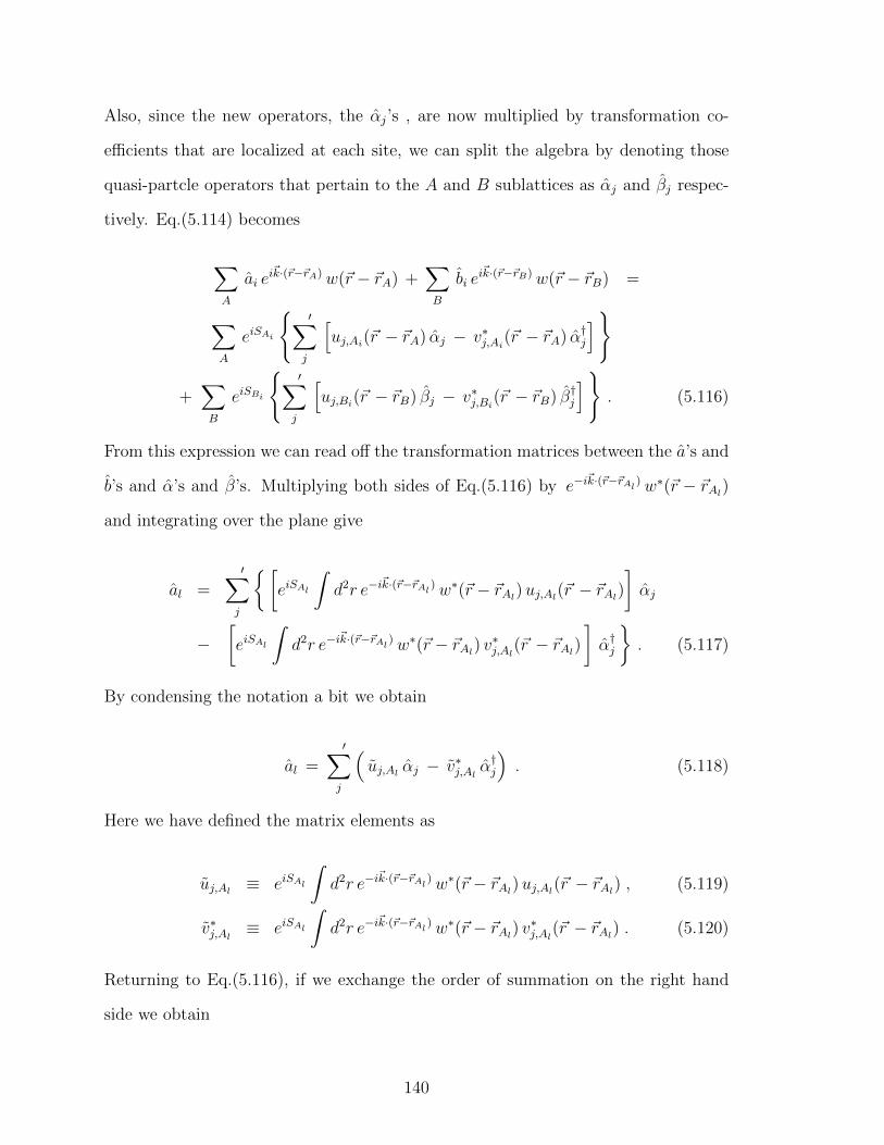
Also, since the new operators, the αj’s , are now multiplied by transformation co-

efficients that are localized at each site, we can split the algebra by denoting those

quasi-partcle operators that pertain to the A and B sublattices as αj and βj respec-

tively. Eq.(5.114) becomes

∑A

ai ei~k·(~r−~rA) w(~r − ~rA) +

∑B

bi ei~k·(~r−~rB) w(~r − ~rB) =

∑A

eiSAi

′∑j

[uj,Ai

(~r − ~rA) αj − v∗j,Ai(~r − ~rA) α†j

]

+∑B

eiSBi

′∑j

[uj,Bi

(~r − ~rB) βj − v∗j,Bi(~r − ~rB) β†j

]. (5.116)

From this expression we can read off the transformation matrices between the a’s and

b’s and α’s and β’s. Multiplying both sides of Eq.(5.116) by e−i~k·(~r−~rAl

) w∗(~r − ~rAl)

and integrating over the plane give

al =′∑j

[eiSAl

∫d2r e−i

~k·(~r−~rAl) w∗(~r − ~rAl

)uj,Al(~r − ~rAl

)

]αj

−[eiSAl

∫d2r e−i

~k·(~r−~rAl) w∗(~r − ~rAl

) v∗j,Al(~r − ~rAl

)

]α†j

. (5.117)

By condensing the notation a bit we obtain

al =′∑j

(uj,Al

αj − v∗j,Alα†j

). (5.118)

Here we have defined the matrix elements as

uj,Al≡ eiSAl

∫d2r e−i

~k·(~r−~rAl) w∗(~r − ~rAl

)uj,Al(~r − ~rAl

) , (5.119)

v∗j,Al≡ eiSAl

∫d2r e−i

~k·(~r−~rAl) w∗(~r − ~rAl

) v∗j,Al(~r − ~rAl

) . (5.120)

Returning to Eq.(5.116), if we exchange the order of summation on the right hand

side we obtain

140

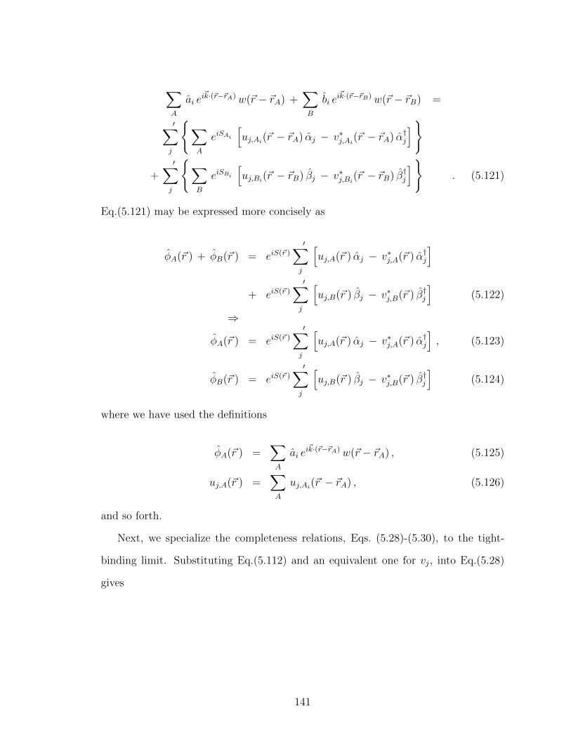
∑A

ai ei~k·(~r−~rA) w(~r − ~rA) +

∑B

bi ei~k·(~r−~rB) w(~r − ~rB) =

′∑j

∑A

eiSAi

[uj,Ai

(~r − ~rA) αj − v∗j,Ai(~r − ~rA) α†j

]

+′∑j

∑B

eiSBi

[uj,Bi

(~r − ~rB) βj − v∗j,Bi(~r − ~rB) β†j

]. (5.121)

Eq.(5.121) may be expressed more concisely as

φA(~r ) + φB(~r ) = eiS(~r )

′∑j

[uj,A(~r ) αj − v∗j,A(~r ) α†j

]+ eiS(~r )

′∑j

[uj,B(~r ) βj − v∗j,B(~r ) β†j

](5.122)

⇒

φA(~r ) = eiS(~r )

′∑j

[uj,A(~r ) αj − v∗j,A(~r ) α†j

], (5.123)

φB(~r ) = eiS(~r )

′∑j

[uj,B(~r ) βj − v∗j,B(~r ) β†j

](5.124)

where we have used the definitions

φA(~r ) =∑A

ai ei~k·(~r−~rA) w(~r − ~rA) , (5.125)

uj,A(~r ) =∑A

uj,Ai(~r − ~rA) , (5.126)

and so forth.

Next, we specialize the completeness relations, Eqs. (5.28)-(5.30), to the tight-

binding limit. Substituting Eq.(5.112) and an equivalent one for vj, into Eq.(5.28)

gives

141

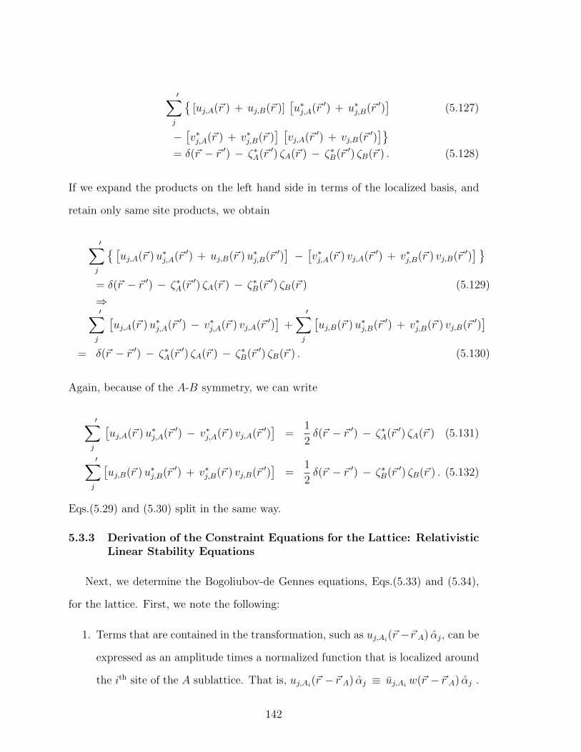
′∑j

[uj,A(~r ) + uj,B(~r )]

[u∗j,A(~r ′) + u∗j,B(~r ′)

](5.127)

−[v∗j,A(~r ) + v∗j,B(~r )

] [vj,A(~r ′) + vj,B(~r ′)

]= δ(~r − ~r ′) − ζ∗A(~r ′) ζA(~r ) − ζ∗B(~r ′) ζB(~r ) . (5.128)

If we expand the products on the left hand side in terms of the localized basis, and

retain only same site products, we obtain

′∑j

[uj,A(~r )u∗j,A(~r ′) + uj,B(~r )u∗j,B(~r ′)

]−[v∗j,A(~r ) vj,A(~r ′) + v∗j,B(~r ) vj,B(~r ′)

] = δ(~r − ~r ′) − ζ∗A(~r ′) ζA(~r ) − ζ∗B(~r ′) ζB(~r ) (5.129)

⇒′∑j

[uj,A(~r )u∗j,A(~r ′) − v∗j,A(~r ) vj,A(~r ′)

]+

′∑j

[uj,B(~r )u∗j,B(~r ′) + v∗j,B(~r ) vj,B(~r ′)

]= δ(~r − ~r ′) − ζ∗A(~r ′) ζA(~r ) − ζ∗B(~r ′) ζB(~r ) . (5.130)

Again, because of the A-B symmetry, we can write

′∑j

[uj,A(~r )u∗j,A(~r ′) − v∗j,A(~r ) vj,A(~r ′)

]=

1

2δ(~r − ~r ′) − ζ∗A(~r ′) ζA(~r ) (5.131)

′∑j

[uj,B(~r )u∗j,B(~r ′) + v∗j,B(~r ) vj,B(~r ′)

]=

1

2δ(~r − ~r ′) − ζ∗B(~r ′) ζB(~r ) . (5.132)

Eqs.(5.29) and (5.30) split in the same way.

5.3.3 Derivation of the Constraint Equations for the Lattice: RelativisticLinear Stability Equations

Next, we determine the Bogoliubov-de Gennes equations, Eqs.(5.33) and (5.34),

for the lattice. First, we note the following:

1. Terms that are contained in the transformation, such as uj,Ai(~r −~r A) αj, can be

expressed as an amplitude times a normalized function that is localized around

the ith site of the A sublattice. That is, uj,Ai(~r − ~r A) αj ≡ uj,Ai

w(~r − ~r A) αj .

142

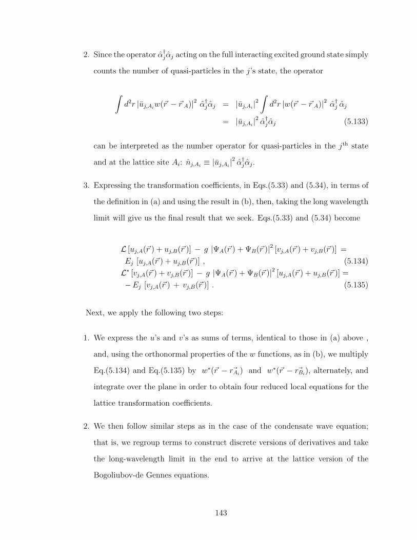
2. Since the operator α†jαj acting on the full interacting excited ground state simply

counts the number of quasi-particles in the j’s state, the operator

∫d2r |uj,Ai

w(~r − ~r A)|2 α†jαj = |uj,Ai|2∫d2r |w(~r − ~r A)|2 α†j αj

= |uj,Ai|2 α†jαj (5.133)

can be interpreted as the number operator for quasi-particles in the jth state

and at the lattice site Ai: nj,Ai≡ |uj,Ai

|2 α†jαj.

3. Expressing the transformation coefficients, in Eqs.(5.33) and (5.34), in terms of

the definition in (a) and using the result in (b), then, taking the long wavelength

limit will give us the final result that we seek. Eqs.(5.33) and (5.34) become

L [uj,A(~r ) + uj,B(~r )] − g |ΨA(~r ) + ΨB(~r )|2 [vj,A(~r ) + vj,B(~r )] =

Ej [uj,A(~r ) + uj,B(~r )] , (5.134)

L∗ [vj,A(~r ) + vj,B(~r )] − g |ΨA(~r ) + ΨB(~r )|2 [uj,A(~r ) + uj,B(~r )] =

−Ej [vj,A(~r ) + vj,B(~r )] . (5.135)

Next, we apply the following two steps:

1. We express the u’s and v’s as sums of terms, identical to those in (a) above ,

and, using the orthonormal properties of the w functions, as in (b), we multiply

Eq.(5.134) and Eq.(5.135) by w∗(~r − ~rAi) and w∗(~r − ~rBi

), alternately, and

integrate over the plane in order to obtain four reduced local equations for the

lattice transformation coefficients.

2. We then follow similar steps as in the case of the condensate wave equation;

that is, we regroup terms to construct discrete versions of derivatives and take

the long-wavelength limit in the end to arrive at the lattice version of the

Bogoliubov-de Gennes equations.

143

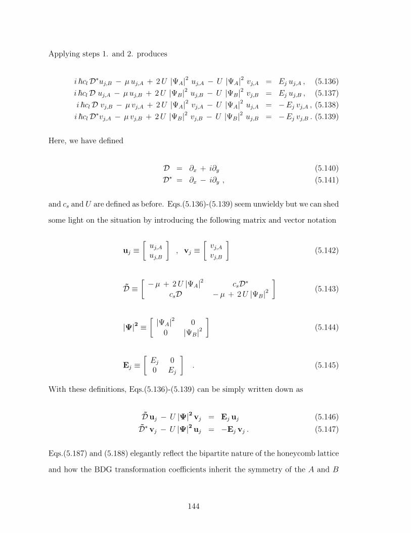
Applying steps 1. and 2. produces

i ~clD∗uj,B − µuj,A + 2U |ΨA|2 uj,A − U |ΨA|2 vj,A = Ej uj,A , (5.136)

i ~clD uj,A − µuj,B + 2U |ΨB|2 uj,B − U |ΨB|2 vj,B = Ej uj,B , (5.137)

i ~clD vj,B − µ vj,A + 2U |ΨA|2 vj,A − U |ΨA|2 uj,A = −Ej vj,A , (5.138)

i ~clD∗vj,A − µ vj,B + 2U |ΨB|2 vj,B − U |ΨB|2 uj,B = −Ej vj,B . (5.139)

Here, we have defined

D = ∂x + i∂y (5.140)

D∗ = ∂x − i∂y , (5.141)

and cs and U are defined as before. Eqs.(5.136)-(5.139) seem unwieldy but we can shed

some light on the situation by introducing the following matrix and vector notation

uj ≡[uj,Auj,B

], vj ≡

[vj,Avj,B

](5.142)

D ≡[−µ + 2U |ΨA|2 csD∗

csD −µ + 2U |ΨB|2]

(5.143)

|Ψ|2 ≡[|ΨA|2 0

0 |ΨB|2]

(5.144)

Ej ≡[Ej 00 Ej

]. (5.145)

With these definitions, Eqs.(5.136)-(5.139) can be simply written down as

D uj − U |Ψ|2 vj = Ej uj (5.146)

D∗ vj − U |Ψ|2 uj = −Ej vj . (5.147)

Eqs.(5.187) and (5.188) elegantly reflect the bipartite nature of the honeycomb lattice

and how the BDG transformation coefficients inherit the symmetry of the A and B

144

sublattice structure. Note also the strong resemblance to the original BDG equations

where the lattice is turned off. It is apparent that the quasi-particles have a spinor-

like structure and that their exact form is determined by substituting a particular

solution for the condensate wavefunction into Eqs.(5.187) and (5.188). As a final

step, we would like to know how the Bogoliubov Hamiltonian, is modified in the

tight-binding limit. We derive the final Hamiltonian by two methods to check the

commutativity of the operations of diagonalizing with respect to the j, k indices

and the α and β indices. The simplest approach is to follow the same steps as the

zero-lattice potential which we have done in the main part of this thesis.

5.4 Calculation of RLSE Eigenvalues and Coherence Factors for a Uni-form Condensate

The wavefunction for a uniform condensate is the single-particle plane wave solu-

tion of the coupled pair of equations

i~cl (∂x + i∂y) ΨA − U |ΨB|2 ΨB + (µ−m)ΨB = 0 (5.148)

i~cl (∂x − i∂y) ΨB − U |ΨA|2 ΨA + (µ−m) ΨA = 0 , (5.149)

where we have included a general mass term m. We can insert the ansatz ΨA(~r ) =

Aei~q·~r and ΨB(~r) = Bei~q·~r, which gives

i~cl (iqx − qy)A− U |B|2B + (µ−m)B = 0 , (5.150)

i~cl (iqx + qy)B − UA3 + (µ−m)A = 0. (5.151)

If we restrict to the uniform density case we can set the spinor amplitudes proportional

to the square root of the average particle density A =√n0 and B = C0

√n0 where

C0 is the phase difference between the upper and lower components. The coupled

equations reduce to

i~cl (iqx − qy)− Un0C0 + (µ − m)C0 = 0 , (5.152)

i~cl (iqx + qy)C0 − U n0 + (µ − m) = 0 . (5.153)

145

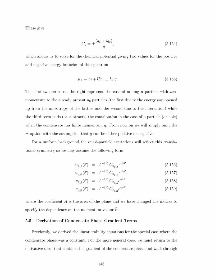
These give

C0 = ±(qx + iqy)

q, (5.154)

which allows us to solve for the chemical potential giving two values for the positive

and negative energy branches of the spectrum

µ± = m+ Un0 ± ~clq. (5.155)

The first two terms on the right represent the cost of adding a particle with zero

momentum to the already present n0 particles (the first due to the energy gap opened

up from the anisotropy of the lattice and the second due to the interaction) while

the third term adds (or subtracts) the contribution in the case of a particle (or hole)

when the condensate has finite momentum q. From now on we will simply omit the

± option with the assumption that q can be either positive or negative.

For a uniform background the quasi-particle excitations will reflect this transla-

tional symmetry so we may assume the following form

u~k,A(~r ) = A−1/2Cu~k,Aei~k·~r, (5.156)

u~k,B(~r ) = A−1/2Cu~k,Bei~k·~r, (5.157)

v~k,A(~r ) = A−1/2Cv~k,Aei~k·~r, (5.158)

v~k,B(~r ) = A−1/2Cv~k,Bei~k·~r, (5.159)

where the coefficient A is the area of the plane and we have changed the indices to

specify the dependence on the momentum vector ~k.

5.5 Derivation of Condensate Phase Gradient Terms

Previously, we derived the linear stability equations for the special case where the

condensate phase was a constant. For the more general case, we must return to the

derivative term that contains the gradient of the condensate phase and walk through

146

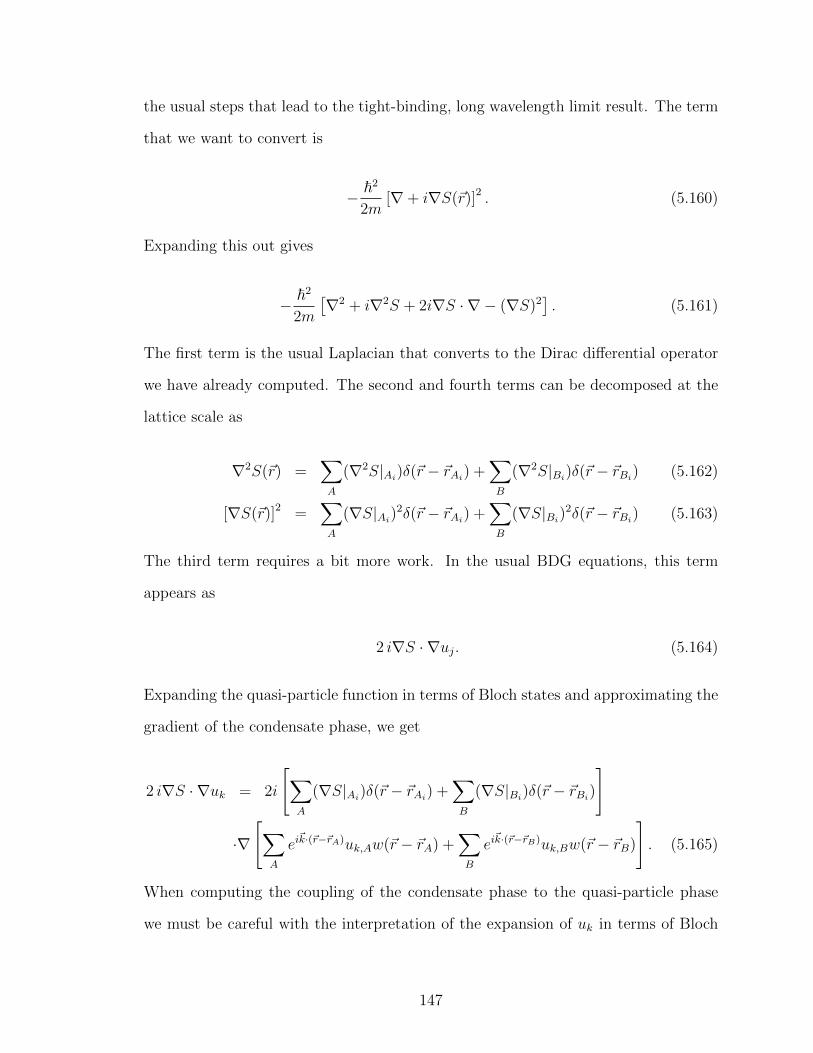
the usual steps that lead to the tight-binding, long wavelength limit result. The term

that we want to convert is

− ~2

2m[∇+ i∇S(~r)]2 . (5.160)

Expanding this out gives

− ~2

2m

[∇2 + i∇2S + 2i∇S · ∇ − (∇S)2

]. (5.161)

The first term is the usual Laplacian that converts to the Dirac differential operator

we have already computed. The second and fourth terms can be decomposed at the

lattice scale as

∇2S(~r) =∑A

(∇2S|Ai)δ(~r − ~rAi

) +∑B

(∇2S|Bi)δ(~r − ~rBi

) (5.162)

[∇S(~r)]2 =∑A

(∇S|Ai)2δ(~r − ~rAi

) +∑B

(∇S|Bi)2δ(~r − ~rBi

) (5.163)

The third term requires a bit more work. In the usual BDG equations, this term

appears as

2 i∇S · ∇uj. (5.164)

Expanding the quasi-particle function in terms of Bloch states and approximating the

gradient of the condensate phase, we get

2 i∇S · ∇uk = 2i

[∑A

(∇S|Ai)δ(~r − ~rAi

) +∑B

(∇S|Bi)δ(~r − ~rBi

)

]

·∇[∑

A

ei~k·(~r−~rA)uk,Aw(~r − ~rA) +

∑B

ei~k·(~r−~rB)uk,Bw(~r − ~rB)

]. (5.165)

When computing the coupling of the condensate phase to the quasi-particle phase

we must be careful with the interpretation of the expansion of uk in terms of Bloch

147

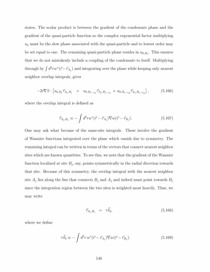
states. The scalar product is between the gradient of the condensate phase and the

gradient of the quasi-particle function so the complex exponential factor multiplying

uk must be the slow phase associated with the quasi-particle and to lowest order may

be set equal to one. The remaining quasi-particle phase resides in uk,Bj. This ensures

that we do not mistakenly include a coupling of the condensate to itself. Multiplying

through by∫d2rw∗(~r−~rAj

) and integrating over the plane while keeping only nearest

neighbor overlap integrals, gives

−2i∇S ·[uk,Bj

~τAj ,Bj+ uk,Bj−n1

~τAj ,Bj−n1+ uk,Bj−n2

~τAj ,Bj−n2

], (5.166)

where the overlap integral is defined as

~τAj ,Bj≡ −

∫d2rw∗(~r − ~rAj

)∇w(~r − ~rBj). (5.167)

One may ask what became of the same-site integrals. These involve the gradient

of Wannier functions integrated over the plane which vanish due to symmetry. The

remaining integral can be written in terms of the vectors that connect nearest neighbor

sites which are known quantities. To see this, we note that the gradient of the Wannier

function localized at site Bj, say, points symmetrically in the radial direction towards

that site. Because of this symmetry, the overlap integral with the nearest neighbor

site Aj lies along the line that connects Bj and Aj and indeed must point towards Bj

since the integration region between the two sites is weighted most heavily. Thus, we

may write

~τAj ,Bj= τ~δ3, (5.168)

where we define

τ~δ3 ≡ −∫d2r w∗(~r − ~rAj

)∇w(~r − ~rBj). (5.169)

148

Similarly,

~τAj ,Bj−n1= τ~δ1 (5.170)

~τAj ,Bj−n2= τ~δ2. (5.171)

We have called the proportionality constant τ and used the same ~δ vectors as before:

~δ1 = ( 12√

3,−1

2) , ~δ2 = ( 1

2√

3, 1

2) , ~δ3 = (− 1√

3, 0) .

Writing this out gives

−2iτ∇S ·(uk,Bj

~δ3 + uk,Bj−n1

~δ1 + uk,Bj−n2

~δ2

). (5.172)

Replacing the on-site quasi-particle c-numbers with the following expressions

uk,Bj= uk,Aj

− ∂~δ3uk,Aj, (5.173)

uk,Bj−n1= uk,Aj

− ∂~δ1uk,Aj, (5.174)

uk,Bj−n2= uk,Aj

− ∂~δ2uk,Aj. (5.175)

We then obtain for Eq. (5.172)

− 2iτ∇S ·[(uk,Aj

− ∂~δ3uk,Aj

)~δ3 +

(uk,Aj

− ∂~δ1uk,Aj

)~δ1 +

(uk,Aj

− ∂~δ2uk,Aj

)~δ2

]= 2iτ∇S ·

(∂~δ3~δ3 + ∂~δ1

~δ1 + ∂~δ2~δ2

)uk,Aj

, (5.176)

where in the second line the uk,Ajterms all vanish due to the symmetry of the δ

vectors. Expressing the partial derivatives in terms of x and y coordinates

∂~δ1 = ~δ1 · ∇ =1

2√

3∂x −

1

2∂y , (5.177)

∂~δ2 = ~δ2 · ∇ =1

2√

3∂x +

1

2∂y , (5.178)

∂~δ3 = ~δ3 · ∇ =−1√

3∂x , (5.179)

149

so that we obtain

2√3iτ∇S ·

[−∂x~δ3 +

(1

2∂x −

√3

2∂y

)~δ1 +

(1

2∂x +

√3

2∂y

)~δ2

]uk,Aj

. (5.180)

Finally, inserting the δ vectors gives

2√3iτ∇S ·

[−∂x

(− 1√

3ex + 0ey

)+

(1

2∂x −

√3

2∂y

)(1

2√

3ex −

1

2ey

)

+

(1

2∂x +

√3

2∂y

)(1

2√

3ex +

1

2ey

)]uk,Aj

=2√3iτ∇S ·

[(1√3∂x +

1

4√

3∂x −

1

4∂y +

1

4√

3∂x +

1

4∂y

)ex

+

(−1

4∂x +

√3

4∂y +

1

4∂x +

√3

4∂y

)ey

]

=2√3iτ∇S ·

(√3

2∂xex +

√3

2∂yey

)= iτ∇S · ∇. (5.181)

The final result returns the gradient but with a factor of τ correction. Next we deter-

mine the transformation of the squared gradient term; the last term in Eq. (5.161).

We must evaluate the expression

(∇S · ∇S)uk,A = (5.182)

(i∇S · i∇S)

[∑A

ei~k·(~r−~rA)uk,Aw(~r − ~rA) +

∑B

ei~k·(~r−~rB)uk,Bw(~r − ~rB)

].

To lowest order we choose to allow one factor of ∇S to vary over a unit cell of the

lattice while approximating the other factor as a constant over one site. As usual

we multiply by the Wannier function for some site and the appropriate exponential

phase factor that contains the lattice momentum. When integrating over the plane,

the dominant terms are ones that are the same-site integrals. We obtain

150

∇S ·∫d2rw∗(~r − ~rA)∇Sw(~r − ~rA) (5.183)

= ∇S ·(τ2∇S|∇S|

)(5.184)

= τ2|∇S|, (5.185)

where, in the second step, we have approximated the integral in that we have written

it proportional to ∇S where τ2 encapsulates the variation of the gradient of S over

the region where the integral has finite support. Eq. (5.161) transforms to

iD∗uk,B +[−i∇SA · ∇+ |∇SA| − i(∇2SA)

]uk,A, (5.186)

where we have omitted dimensionful factors which must, in the end, be compared to

justify the inherent assumption that all terms are of comparable order. The linear

stability equations become

i ~clD∗uj,B +QAuj,A + 2U |ΨA|2 uj,A − U |ΨA|2 vj,A = Ejuj,A , (5.187)

i ~clDuj,A +QBuj,B + 2U |ΨB|2 uj,B − U |ΨB|2 vj,B = Ejuj,B , (5.188)

i ~clD∗vj,B +Q∗Avj,A + 2U |ΨA|2 vj,A − U |ΨA|2 uj,A = −Ejvj,A , (5.189)

i ~clDvj,A +Q∗Bvj,B + 2U |ΨB|2 vj,B − U |ΨB|2 uj,B = −Ejvj,B , (5.190)

where we define

QA(B) =[m− µ− i∇SA(B) · ∇+ |∇SA(B)| − i(∇2SA(B))

]. (5.191)

5.6 Energy Eigenvalues

Substituting for the plane wave condensate and quasi-particle states, Eqs. (5.187)-

(5.190) become

151

(n0U − Ek + ~q · ~k)Cu~k,A − κ∗Cu~k,B − n0UCv~k,A + (0)Cv~k,B = 0 , (5.192)

−κCu~k,A + (n0U − Ek + ~q · ~k)Cu~k,B + (0)Cv~k,A − n0UCv~k,B = 0 , (5.193)

−n0UCu~k,A + (0)Cu~k,B + (n0U + Ek − ~q · ~k)Cv~k,A − κ∗Cv~k,B = 0 , (5.194)

(0)Cu~k,A − n0UCu~k,B − κCv~k,A + (n0U + Ek − ~q · ~k)Cv~k,B = 0 , (5.195)

where for compactness we write κ ≡ (kx+iky). The coefficients of the complex ampli-

tudes Cu~k,A , Cu~k,B , Cv~k,A , and Cv~k,B form a 4x4 matrix whose determinant set equal

to zero yields the four eigenvalues of the system: E(1)k , E

(2)k , E

(3)k , E

(4)k . The possible

presence of complex eigenvalues will determine the stability of the condensate with

decay rates out of the condensate through the various modes being proportional to

the magnitudes of the imaginary parts. We compute the determinant of the coefficient

matrix

det

E− −κ∗ −n0U 0−κ E− 0 −n0U−n0U 0 E+ −κ∗

0 −n0U −κ E+

= 0, , (5.196)

where we have used the short hand notation E± =[n0U ± (Ek − ~q · ~k)

]. Computing

the determinant we obtain

E−[E−(E+2 − κ2)− E+(n0U)2

]+ κ∗

[−κ(E+2 − κ2)− κn0U

]−n0U

[κ2n0U + E−E+n0U − (n0U)3

]= 0 , (5.197)

where we use the notation κ2 ≡ κ∗κ. Multiplying this out gives

E−2E+2 − κ2(E−

2+ E+2

)− 2E−E+(n0U)2 − 2κ2(n0U)2 + κ4 + (n0U)4 = 0 . (5.198)

To further simplify the calculation we define E± = (x±y), then Eq. (5.198) simplifies

to

152

(x2 − y2)2 − 2κ2(x2 + y2)− 2(n0U)2(x2 − y2)− 2κ2(n0U)2 + κ4 + (n0U)4 = 0 . (5.199)

Gathering quadratic and quartic terms in y,

y4 + 2[(n0U)2 − x2 − κ2

]y2

+[x4 − 2κ2x2 − 2(n0U)2x2 − 2κ2(n0U)2 + κ4 + (n0U)4

]= 0 , (5.200)

and solving for y2,

y2 = −[(n0U)2 − x2 − κ2

]±[(n0U)4 + κ4 + x4 − 2κ2(n0U)2 (5.201)

− 2x2(n0U)2 + 2κ2x2 − x4 + 2κ2x2 + 2x2(n0U)2 + 2κ2(n0U)2 − κ4 − (n0U)4]1/2

.

With y = Ek−~q ·~k and x = n0U , and the explicit definition of κ, the eigenvalues are

Ek = ~q · ~k ±√k2 ± 2n0Uk . (5.202)

For reasons that we will discuss later, we will retain only the positive option that

appears under the radical sign. Thus, the energy spectrum is

Ek = ~q · ~k ±√k2 + 2n0Uk . (5.203)

Reinserting the dimensionful physical constants gives

Ek = c′l~~q · ~k ±√

(cl~k)2 + n0Ucl~k , (5.204)

or in keeping with the usual Bogoliubov notation found in the literature, we may

write

Ek = (c′l/cl)~q · ~εk0 ± E0k , (5.205)

E0k =

√(ε0k)

2 + n0gε0k , (5.206)

153

where ε0k = cl~k is the single quasi-particle energy for zero interaction, E0k is the

quasi-particle energy for a static background,

cl =

√3tha

2~, (5.207)

c′l =

√3τa

2~. (5.208)

Recalling that cl has dimensions of velocity while c′l has dimensions of m2 · s−1, since

τ is an integral over the gradient instead of the Laplacian. The form of the energy

changes from a linear dependence on k to a a dependence on k1/2, the two regions

separated by the condition cl~k/n0U ≈ 1. From this we may define the modified

coherence length as

ξ′ =cl~n0U

. (5.209)

5.7 Limits of Quasi-Particle Energy

1. Uniform background q → 0. For the case of zero condensate momentum, q = 0,

we obtain

Ek = ±E0k = ±

√(cl~k)2 + n0Ucl~k , (5.210)

or,

Ek = ±cl~k(

1 +n0U

cl~k

)1/2

. (5.211)

We may examine the two limits: short wavelength, k ξ′−1, and long wave-

length, k ξ′−1. In the short wavelength limit E(±)k = ±cl~k + n0U/2. This

is the expected result for particle like excitations, i.e., lattice potential but no

contact interaction, shifted by a mean-field Hartree term for the interaction

with the background condensate. For these excitations the momentum is too

154

large for the contact interaction to be noticed except in the form of a mean-field

interaction. In the long wavelength limit, the second term dominates so that

we obtain

E(±)k = ±ξ′−1/2k1/2. (5.212)

The first thing we notice is that the energy depends on momentum as k1/2.

These are low-energy collective modes; excitations just above the condensate

energy.

2. Zero-interaction n0U → 0 . If we turn off the interaction, the quasi-particle

energy reduces to

Ek = c′l~~q · ~k ± cl~k . (5.213)

These are excitations of the noninteracting condensate where the first term

describes the anisotropy due to the motion of the condensate and the second

term is the usual linear dispersion for the honeycomb lattice.

3. Zero-limit check of quasi-particle momentum k → 0. If we set k to zero we

should expect Ek to go to zero which is indeed the case.

5.7.1 Directional Behavior of the Energy

The dot product of ~q and ~k that appears in the energy is the counterpart of the

term that appears in the Bogoliubov dispersion for a moving condensate. This term

gives an anisotropic distribution for the energy for a particular direction determined

by ~q and implies a stability critical angle θc. Some of these modes have negative

energy so that the condensate may arbitrarily lower its energy through such emissions

(these are usually called energetic instabilities in the literature.) The energy may be

expressed in terms of the relative angle θ between ~q and ~k

155

Ek = c′l~qk cosθ ±√

(cl~k)2 + n0Ucl~k , (5.214)

where the critical angle may be obtained by setting the energy to zero for fixed ~q and

~k. The energy may be expressed as

Ek = ~k [vcosθ ± s(k)] , (5.215)

where v = ~c′lq is the speed of the condensate and the momentum dependent “speed

of light” is defined as

s(k) = cl

√1 +

n0U

cl~k. (5.216)

From this expression the two regimes are evident. In the “particle” regime (k

n0U/cl~) s reduces to the usual effective speed of light s ≈ cl for a condensate

in a honeycomb lattice. In the “phonon” regime (k n0U/cl~) we have s(k) ≈√cln0U/~k (we have used quotations here since “particle” and “phonon” are more

appropriate for the usual weakly interacting Bose gas where no lattice is present).

For the first case, the energy is approximately

Ek ≈ ~k (vcosθ ± cl) . (5.217)

Assuming a positive velocity for the condensate, we see that the sign of Ek depends

on the direction of quasi-particle emission as well as whether the quasi-particle is a

positive or negative energy excitation. For positive energy modes, the condensate is

stable if

v

clcosθ + 1 ≥ 0. (5.218)

156

If v < cl, positive energy modes are always stable regardless of the angle of emission.

For v ≥ cl, there is a critical angle beyond which all positive modes are unstable

determined by

θc = cos−1(−cl/v), (5.219)

from which we can see that for the limiting case v cl, we have θc ≈ π/2 so that

emission of positive modes in the half sphere in the backwards direction are unstable.

When the condensate speed is equal to the speed of light, v = cl, then we find θc ≈ π.

This marks the onset of instability. Here only emissions in the opposite direction of

~q are unstable.

As one would expect, the situation is quite different in the case of negative energy

excitations. The stability condition reads

v

clcosθ − 1 ≥ 0. (5.220)

First, we see that when v < cl, all negative energy modes are unstable. For the case

v ≥ cl, the energy is stable for certain angles with θc determined by

θc = cos−1(cl/v). (5.221)

This condition is identical to the case of positive excitations except that now θc marks

the onset of instability for a wider range of emission directions. For the limiting case

v cl, we find θc = π/2 where we see that for very large condensate speeds, emissions

of negative energy modes in the forward directions are actually stable. For the case

where v = cl we find that θc = 0. This is marks the point where all negative energy

modes become unstable.

157

5.8 Coherence Factors for Uniform Background

Now we compute the coefficients Cv~k,A and Cv~k,B for the simplest case where ~q = 0

by solving the system of equations

(n0U − Ek)Cu~k,A − κ∗Cu~k,B − n0UCv~k,A + (0)Cv~k,B = 0 , (5.222)

−κCu~k,A + (n0U − Ek)Cu~k,B + (0)Cv~k,A − n0UCv~k,B = 0 , (5.223)

−n0UCu~k,A + (0)Cu~k,B + (n0U + Ek)Cv~k,A − κ∗Cv~k,B = 0 , (5.224)

(0)Cu~k,A − n0U Cu~k,B − κCv~k,A + (n0U + Ek)Cv~k,B = 0 . (5.225)

For a particular choice of the normalization conditions, we have

∫d2r[u∗~j,A(~r)u~k,A(~r)− v∗~j,A(~r)v~k,A(~r)

]= δ~j,~k , (5.226)∫

d2r[u∗~j,B(~r)u~k,B(~r)− v∗~j,B(~r)v~k,B(~r)

]= δ~j,~k . (5.227)

This implies for the coefficients

|Cu~k,A|2 = 1 + |Cv~k,A|

2 , (5.228)

|Cu~k,B |2 = 1 + |Cv~k,B |

2 . (5.229)

In all we have six equations and eight unknowns (four complex coefficients). Writing

the coefficients in terms of amplitude and phase and setting two of the phases to

unity

Cu~k,A = |Cu~k,A| , (5.230)

Cu~k,B = |Cu~k,B |eiφu , (5.231)

Cv~k,A = |Cu~k,A| , (5.232)

Cv~k,B = |Cu~k,B |eiφv . (5.233)

We must solve

158

(n0U − Ek)|Cu~k,A| − κ∗|Cu~k,B |e

iφu − n0U |Cv~k,A|+ (0)|Cv~k,B |eiφv = 0, (5.234)

−κ|Cu~k,A|+ (n0U − Ek)|Cu~k,B |eiφu + (0)|Cv~k,A| − n0U |Cv~k,B |e

iφv = 0, (5.235)

−n0U |Cu~k,A|+ (0)|Cu~k,B |eiφu + (n0U + Ek)|Cv~k,A| − κ

∗|Cv~k,B |eiφv = 0, (5.236)

(0)|Cu~k,A| − n0U |Cu~k,B |eiφu − κ|Cv~k,A|+ (n0U + Ek)|Cv~k,B |e

iφv = 0. (5.237)

Adding Eqs. (5.234) and (5.236) gives

−Ek|Cu~k,A| − κ∗|Cu~k,B |e

iφu + Ek|Cv~k,A| − κ∗|Cv~k,B |e

iφv = 0 . (5.238)

Adding Eqs. (5.235) and (5.237) gives

−κ|Cu~k,A| − Ek|Cu~k,B |eiφu − κ|Cv~k,A|+ Ek|Cv~k,B |e

iφv = 0. (5.239)

Regrouping terms in both equations gives

−κ∗(|Cu~k,B |eiφu + |Cv~k,B |e

iφv) = Ek|Cu~k,A| − Ek|Cv~k,A| , (5.240)

−κ(|Cu~k,A|+ |Cv~k,A|) = Ek|Cu~k,B |eiφu − Ek|Cv~k,B |e

iφv . (5.241)

Multiplying these equations gives

k2(|Cu~k,B |eiφu + |Cv~k,B |e

iφv)(|Cu~k,A|+ |Cv~k,A|) =[Ek|Cu~k,A| − Ek|Cv~k,A|

]×[Ek|Cu~k,B |e

iφu − Ek|Cv~k,B |eiφv]. (5.242)

The kinetic part of the Hamiltonian mixes A and B sublattice components so we are

free to decouple the corresponding coefficients by taking

k(|Cu~k,A|+ |Cv~k,A|) = Ek|Cu~k,A| − Ek |Cv~k,A| , (5.243)

k(|Cu~k,B |eiφu + |Cv~k,B |e

iφv) = Ek|Cu~k,B |eiφu − Ek|Cv~k,B |e

iφv . (5.244)

Combining like terms gives

159

(Ek − k)|Cu~k,A| = (Ek + k)|Cv~k,A| , (5.245)

(Ek − k)|Cu~k,B |ei(φu−φv) = (Ek+, k)|Cv~k,B | . (5.246)

Equating the phases on both sides gives φu = φv ≡ φ. Squaring both sides of each

equation and inserting the normalization constraints, we get

(Ek − k)2(1 + |Cv~k,A|2) = (Ek + k)2|Cv~k,A|

2 (5.247)

(Ek − k)2(1 + |Cv~k,B |2) = (Ek + k)2|Cv~k,B |

2, (5.248)

which yields the solutions

|Cv~k,A| =(Ek − k)

2(Ekk)1/2, (5.249)

|Cu~k,A| = (1 + |Cv~k,A|2)1/2 , (5.250)

=(Ek + k)

2 (Ekk)1/2, (5.251)

with identical solutions for the B sublattice. Inserting the dimensionful constants,

we may label the energy eigenvalues by

E(+)k = +

√(~cl~ k)2 + n0Ucl~k = +E0

k , (5.252)

E(−)k = −

√(~cl~ k)2 + n0Ucl~k = −E0

k , (5.253)

and we define

C(±,±) =(E

(±)k ± cl~k)

2(E(±)k cl~k)1/2

, (5.254)

w =

(1eiφ

). (5.255)

Then the quasi-particle states are

160

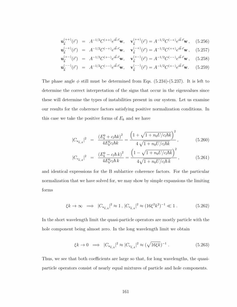
u(++)~k

(~r ) = A−1/2C(++)ei~k·~rw, v

(++)~k

(~r ) = A−1/2C(−+)ei~k·~rw , (5.256)

u(−+)~k

(~r ) = A−1/2C(−+)ei~k·~rw, v

(−+)~k

(~r ) = A−1/2C(++)ei~k·~rw , (5.257)

u(+−)~k

(~r ) = A−1/2C(+−)ei~k·~rw, v

(+−)~k

(~r ) = A−1/2C(−−)ei~k·~rw , (5.258)

u(−−)~k

(~r ) = A−1/2C(−−)ei~k·~rw, v

(−−)~k

(~r ) = A−1/2C(+−)ei~k·~rw. (5.259)

The phase angle φ still must be determined from Eqs. (5.234)-(5.237). It is left to

determine the correct interpretation of the signs that occur in the eigenvalues since

these will determine the types of instabilities present in our system. Let us examine

our results for the coherence factors satisfying positive normalization conditions. In

this case we take the positive forms of Ek and we have

|Cu~k,A|2 =

(E0k + cl~k)

2

4E0kcl~k

=

(1 +

√1 + n0U/cl~k

)2

4√

1 + n0U/cl~k, (5.260)

|Cv~k,A|2 =

(E0k − cl~ k)

2

4E0kcl~ k

=

(1−

√1 + n0U/cl~k

)2

4√

1 + n0U/cl~ k, (5.261)

and identical expressions for the B sublattice coherence factors. For the particular

normalization that we have solved for, we may show by simple expansions the limiting

forms

ξk →∞ =⇒ |Cu~k,A|2 ≈ 1 , |Cv~k,A|

2 ≈ (16ξ2k2)−1 1 . (5.262)

In the short wavelength limit the quasi-particle operators are mostly particle with the

hole component being almost zero. In the long wavelength limit we obtain

ξk → 0 =⇒ |Cu~k,A|2 ≈ |Cv~k,A|

2 ≈ (√

16ξk)−1 . (5.263)

Thus, we see that both coefficients are large so that, for long wavelengths, the quasi-

particle operators consist of nearly equal mixtures of particle and hole components.

161

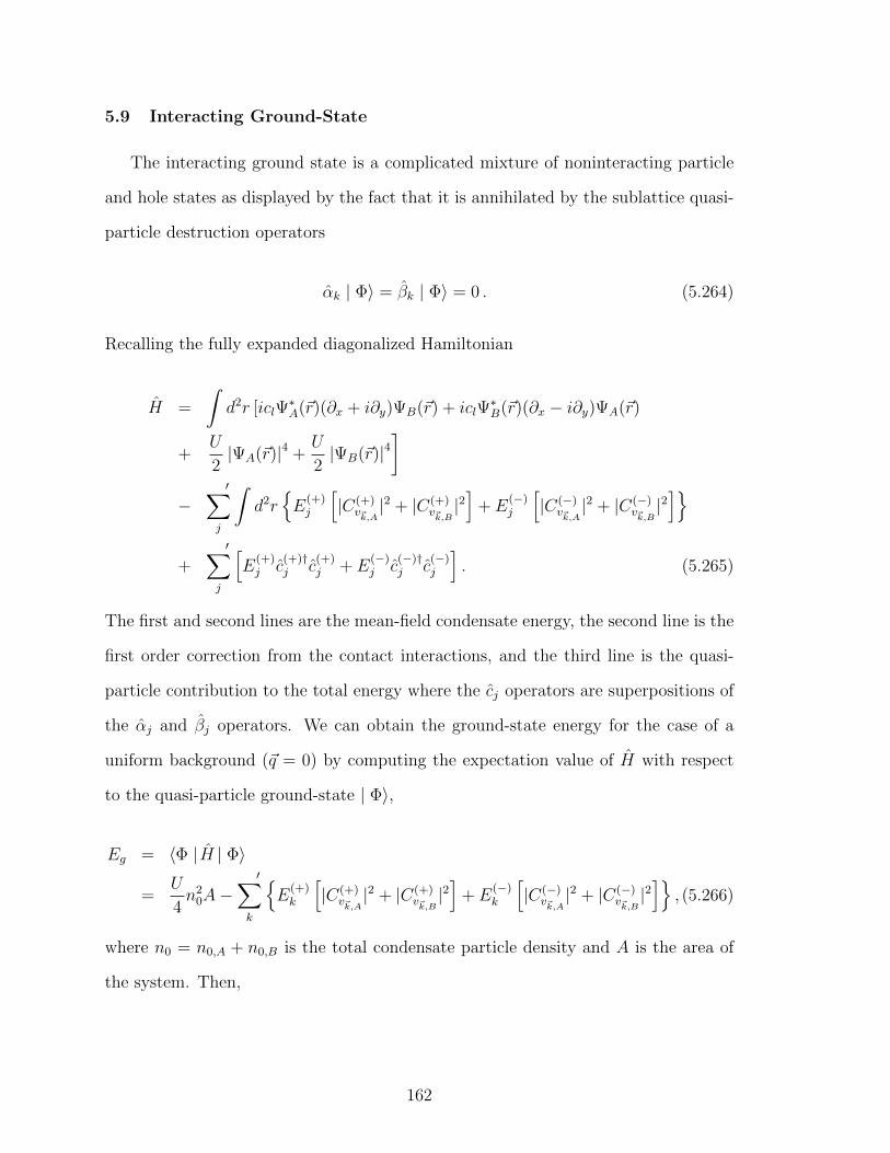
5.9 Interacting Ground-State

The interacting ground state is a complicated mixture of noninteracting particle

and hole states as displayed by the fact that it is annihilated by the sublattice quasi-

particle destruction operators

αk | Φ〉 = βk | Φ〉 = 0 . (5.264)

Recalling the fully expanded diagonalized Hamiltonian

H =

∫d2r [iclΨ

∗A(~r)(∂x + i∂y)ΨB(~r) + iclΨ

∗B(~r)(∂x − i∂y)ΨA(~r)

+U

2|ΨA(~r)|4 +

U

2|ΨB(~r)|4

]−

′∑j

∫d2rE

(+)j

[|C(+)

v~k,A|2 + |C(+)

v~k,B|2]

+ E(−)j

[|C(−)

v~k,A|2 + |C(−)

v~k,B|2]

+′∑

j

[E

(+)j c

(+)†j c

(+)j + E

(−)j c

(−)†j c

(−)j

]. (5.265)

The first and second lines are the mean-field condensate energy, the second line is the

first order correction from the contact interactions, and the third line is the quasi-

particle contribution to the total energy where the cj operators are superpositions of

the αj and βj operators. We can obtain the ground-state energy for the case of a

uniform background (~q = 0) by computing the expectation value of H with respect

to the quasi-particle ground-state | Φ〉,

Eg = 〈Φ |H | Φ〉

=U

4n2

0A−′∑

k

E

(+)k

[|C(+)

v~k,A|2 + |C(+)

v~k,B|2]

+ E(−)k

[|C(−)

v~k,A|2 + |C(−)

v~k,B|2]

, (5.266)

where n0 = n0,A + n0,B is the total condensate particle density and A is the area of

the system. Then,

162

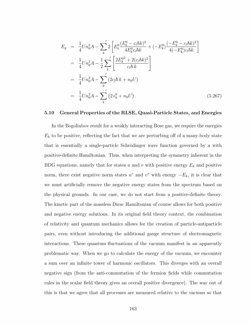
Eg =1

4Un2

0A−′∑

k

2

[E0k

(E0k − cl~k)2

4E0kcl~k

+ (−E0k)

(−E0k − cl~k)2

4(−E0k)cl~k

]

=1

4Un2

0A−1

2

′∑k

[2E0

k2

+ 2(cl~k)2

cl~ k

]

=1

4Un2

0A−′∑

k

(2cl~ k + n0U)

=1

4Un2

0A−′∑

k

(2 ε0k + n0U

). (5.267)

5.10 General Properties of the RLSE, Quasi-Particle States, and Energies

In the Bogoliubov result for a weakly interacting Bose gas, we require the energies

Ek to be positive, reflecting the fact that we are perturbing off of a many-body state

that is essentially a single-particle Schrodinger wave function governed by a with

positive-definite Hamiltonian. Thus, when interpreting the symmetry inherent in the

BDG equations, namely that for states u and v with positive energy Ek and positive

norm, there exist negative norm states u∗ and v∗ with energy −Ek, it is clear that

we must artificially remove the negative energy states from the spectrum based on

the physical grounds. In our case, we do not start from a positive-definite theory.

The kinetic part of the massless Dirac Hamiltonian of course allows for both positive

and negative energy solutions. In its original field theory context, the combination

of relativity and quantum mechanics allows for the creation of particle-antiparticle

pairs, even without introducing the additional gauge structure of electromagnetic

interactions. These quantum fluctuations of the vacuum manifest in an apparently

problematic way. When we go to calculate the energy of the vacuum, we encounter

a sum over an infinite tower of harmonic oscillators. This diverges with an overall

negative sign (from the anti-commutation of the fermion fields while commutation

rules in the scalar field theory gives an overall positive divergence). The way out of

this is that we agree that all processes are measured relative to the vacuum so that

163

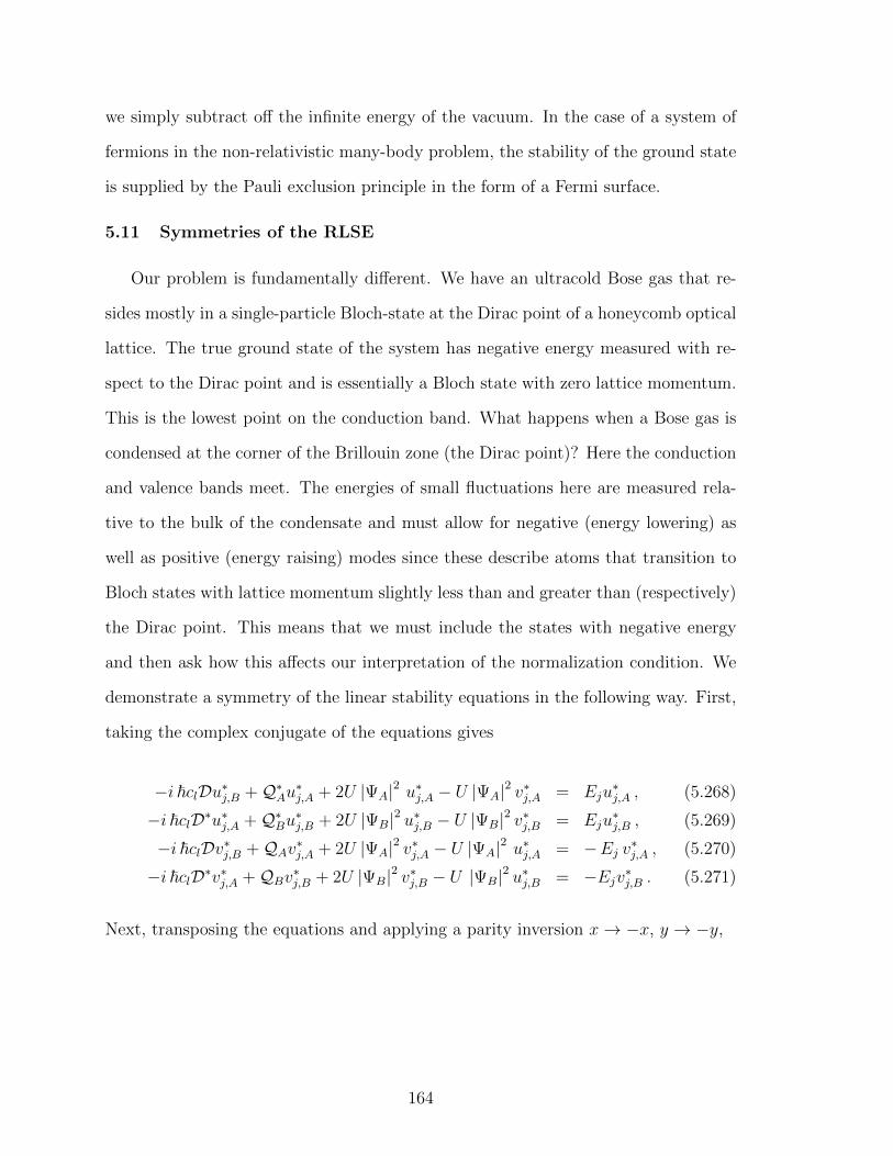
we simply subtract off the infinite energy of the vacuum. In the case of a system of

fermions in the non-relativistic many-body problem, the stability of the ground state

is supplied by the Pauli exclusion principle in the form of a Fermi surface.

5.11 Symmetries of the RLSE

Our problem is fundamentally different. We have an ultracold Bose gas that re-

sides mostly in a single-particle Bloch-state at the Dirac point of a honeycomb optical

lattice. The true ground state of the system has negative energy measured with re-

spect to the Dirac point and is essentially a Bloch state with zero lattice momentum.

This is the lowest point on the conduction band. What happens when a Bose gas is

condensed at the corner of the Brillouin zone (the Dirac point)? Here the conduction

and valence bands meet. The energies of small fluctuations here are measured rela-

tive to the bulk of the condensate and must allow for negative (energy lowering) as

well as positive (energy raising) modes since these describe atoms that transition to

Bloch states with lattice momentum slightly less than and greater than (respectively)

the Dirac point. This means that we must include the states with negative energy

and then ask how this affects our interpretation of the normalization condition. We

demonstrate a symmetry of the linear stability equations in the following way. First,

taking the complex conjugate of the equations gives

−i ~clDu∗j,B +Q∗Au∗j,A + 2U |ΨA|2 u∗j,A − U |ΨA|2 v∗j,A = Eju∗j,A , (5.268)

−i ~clD∗u∗j,A +Q∗Bu∗j,B + 2U |ΨB|2 u∗j,B − U |ΨB|2 v∗j,B = Eju∗j,B , (5.269)

−i ~clDv∗j,B +QAv∗j,A + 2U |ΨA|2 v∗j,A − U |ΨA|2 u∗j,A = −Ej v∗j,A , (5.270)

−i ~clD∗v∗j,A +QBv∗j,B + 2U |ΨB|2 v∗j,B − U |ΨB|2 u∗j,B = −Ejv∗j,B . (5.271)

Next, transposing the equations and applying a parity inversion x→ −x, y → −y,

164

i ~clD∗v∗j,A +QBv∗j,B + 2U |ΨB|2 v∗j,B − U |ΨB|2 u∗j,B = −Ejv∗j,B , (5.272)

i ~clDv∗j,B +QAv∗j,A + 2U |ΨA|2 v∗j,A − U |ΨA|2 u∗j,A = −Ejv∗j,A , (5.273)

i ~clD∗u∗j,A +Q∗Bu∗j,B + 2U |ΨB|2 u∗j,B + U |ΨB|2 v∗j,B = Eju∗j,B , (5.274)

i ~clDu∗j,B +Q∗Au∗j,A + 2U |ΨA|2 u∗j,A − U |ΨA|2 v∗j,A = Eju∗j,A .. (5.275)

Finally, exchanging A and B sublattice labels along with the field redefinitions

u′j,B = v∗j,A , (5.276)

u′j,A = v∗j,B , (5.277)

v′j,B = u∗j,A , (5.278)

v′j,A = u∗j,B , (5.279)

we obtain

i ~clD∗u′j,B +QAu′j,A + 2U |ΨA|2 u′j,A − U |ΨA|2 v′j,A = E ′ju′j,A , (5.280)

i ~clDu′j,A +QBu′j,B + 2U |ΨB|2 u′j,B − U |ΨB|2 v′j,B = E ′juj,B , (5.281)

i ~clD∗v′j,B +Q∗Av′j,A + 2U |ΨA|2 v′j,A − U |ΨA|2 u′j,A = −E ′jv′j,A , (5.282)

i ~clDv′j,A +Q∗Bv′j,B + 2U |ΨB|2 v′j,B − U |ΨB|2 u′j,B = −E ′jv′j,B, (5.283)

where we define the new energy as E ′j ≡ −Ej. These equations are identical to the

original ones except that the sign of the energy is flipped. This is positive/negative

energy symmetry for the space of excitations and (unlike the BDG problem) here must

be respected since we are measuring energy relative to the Dirac point as previously

discussed. For the simple case of a plane wave background, this is the obvious result

that inverting the direction of positive momentum Dirac-like particles (the parity

inversion in the derivative terms) yields the negative energy branch of the spectrum.

5.12 Normalization of Quasi-Particle States

The normalization for the positive and negative energy solutions may be derived

from the linear stability equations. Beginning with Eq. (5.188), we multiply through

165

by u∗k,B,

iu∗k,BDuk,A +QBu∗k,Buj,B + 2U |ΨB|2 u∗k,Buj,B − U |ΨB|2 u∗k,Bvj,B= Eju

∗k,Buj,B. (5.284)

Next, we take the complex conjugate and exchange j and k indices which yields

−iuj,BD∗u∗k,A +Q∗Buj,Bu∗k,B + 2U |ΨB|2 uj,Bu∗k,B − U |ΨB|2 uj,Bv∗k,B= E∗kuj,Bu

∗k,B, (5.285)

where we have allowed the possibility that the energy is complex. Subtracting

Eq. (5.285) from Eq. (5.284) and integrating over the plane gives

i

∫d2r(u∗k,BDuk,A + uj,BD∗u∗k,A

)+ (QB −Q∗B)

∫d2ru∗k,Buj,B

+ U

∫d2r |ΨB|2

(uj,Bv

∗k,B − u∗k,Bvj,B

)= (Ej − E∗k)

∫d2ru∗k,Buj,B. (5.286)

Following the same steps for Eq. (5.190) yields a similar equation

− i

∫d2r(v∗k,BDvk,A + vj,BD∗v∗k,A

)+ (QB −Q∗B)

∫d2rv∗k,Bvj,B

+ U

∫d2r |ΨB|2

(uj,Bv

∗k,B − u∗k,Bvj,B

)= (Ej − E∗k)

∫d2rv∗k,Bvj,B. (5.287)

Subtracting these two results and taking ∇2S = 0, we get

i

∫d2r(u∗k,BDQAuk,A + uj,BD∗Q∗Au∗k,A + v∗k,BDQAvk,A + vj,BD∗Q∗Av∗k,A

)= (Ej − E∗k)

∫d2r(u∗k,Buj,B − v∗k,Bvj,B

). (5.288)

A similar equation is obtained by manipulating Eq. (5.187) and Eq. (5.189)

i

∫d2r(u∗k,AD∗Q∗Buk,B + uj,ADQBu∗k,B + v∗k,AD∗Q∗Bvk,B + vj,ADQBv∗k,B

)= (Ej − E∗k)

∫d2r(u∗k,Auj,A − v∗k,Avj,A

). (5.289)

166

Adding these equations gives

i

∫d2r(u∗k,AD∗Q∗Buk,B + uj,ADQBu∗k,B + v∗k,AD∗Q∗Bvk,B + vj,ADQBv∗k,B

)+ i

∫d2r(u∗k,AD∗Q∗Buk,B + uj,ADQBu∗k,B + v∗k,AD∗Q∗Bvk,B + vj,ADQBv∗k,B

)= (Ej − E∗k)

∫d2r(u∗k,Auj,A − v∗k,Avj,A + u∗k,Buj,B − v∗k,Bvj,B

). (5.290)

By using properties of the derivative terms, the left hand side can be made to vanish

so that we may write

(Ej − E∗k)∫d2r(u∗k,Auj,A − v∗k,Avj,A + u∗k,Buj,B − v∗k,Bvj,B

)= 0. (5.291)

This is the expected normalization condition similar to the BDG case.

5.13 Positive and Negative Energy States: Lattice Versus InteractionEffects

In our problem, the number of possible states is expanded since the normalization

couples A and B states. For nonzero normalization constant, we see that by setting

j = k, the energy must be real and the normalization condition can be expressed as

∫d2r(u∗k,Auj,A − v∗k,Avj,A + u∗k,Buj,B − v∗k,Bvj,B

)= δjk. (5.292)

In order for the quasi-particle operator to obey the usual Bose commutation rela-

tions (as we have already seen), we are allowed positive as well as negative energy

solutions provided the normalization constant for these states is positive and negative

respectively. The presence of negative norm states introduces no physical inconsis-

tency but a minor reinterpretation of the Fourier components is needed. Requiring

Bosonic commutation rules for the quasi-particle part of the wavefunction forces the

condition

(|uj|2 − |vj|2

) [αj, α

†j

]= 1. (5.293)

167

If we take (|uj|2 − |vj|2) = −1, this forces[αj, α

†j

]= −1 or,

[α†j, αj

]= 1 so that

we must interpret α†j and αj as the destruction and creation operators, respectively,

for a Boson (quasi-hole) with momentum −j which are of course the negative energy

states of our theory. Thus, for negative energy states, we require that

∫d2r(u∗k,Auj,A − v∗k,Avj,A + u∗k,Buj,B − v∗k,Bvj,B

)= −δjk. (5.294)

Since excitations of the two sublattices are not normalized independently, as seen in

Eq. (5.292) and Eq. (5.294), there exists the possibility for solutions that appear as

holes in one sublattice and particles in the other while the total energy is fixed positive

or negative. To elaborate on this, the fact that Eq. (5.292) shows that sublattice

amplitudes are not independently normalized, means that the amplitudes u and v for

one of the sublattices, say B, may appear as a hole (negative normalization for that

sublattice)

∫d2r(u∗k,Buj,B − v∗k,Bvj,B

)= −δjk , (5.295)

forcing the other two amplitudes (for the A sublattice) to be positively normalized

but multiplied by a factor of 2:

∫d2r(u∗k,Auj,A − v∗k,Avj,A

)= 2δjk . (5.296)

This means that for positive Ej (quasi-particle propagation), one sublattice may

appear to support two quasi-particles while the other sublattice supporting one quasi-

hole. There also exists the possibility of zero norm states in which case the energy may

be complex. Some representative characteristics of the possible states are summarized

in Table 5.1 and Table 5.2 below.

168

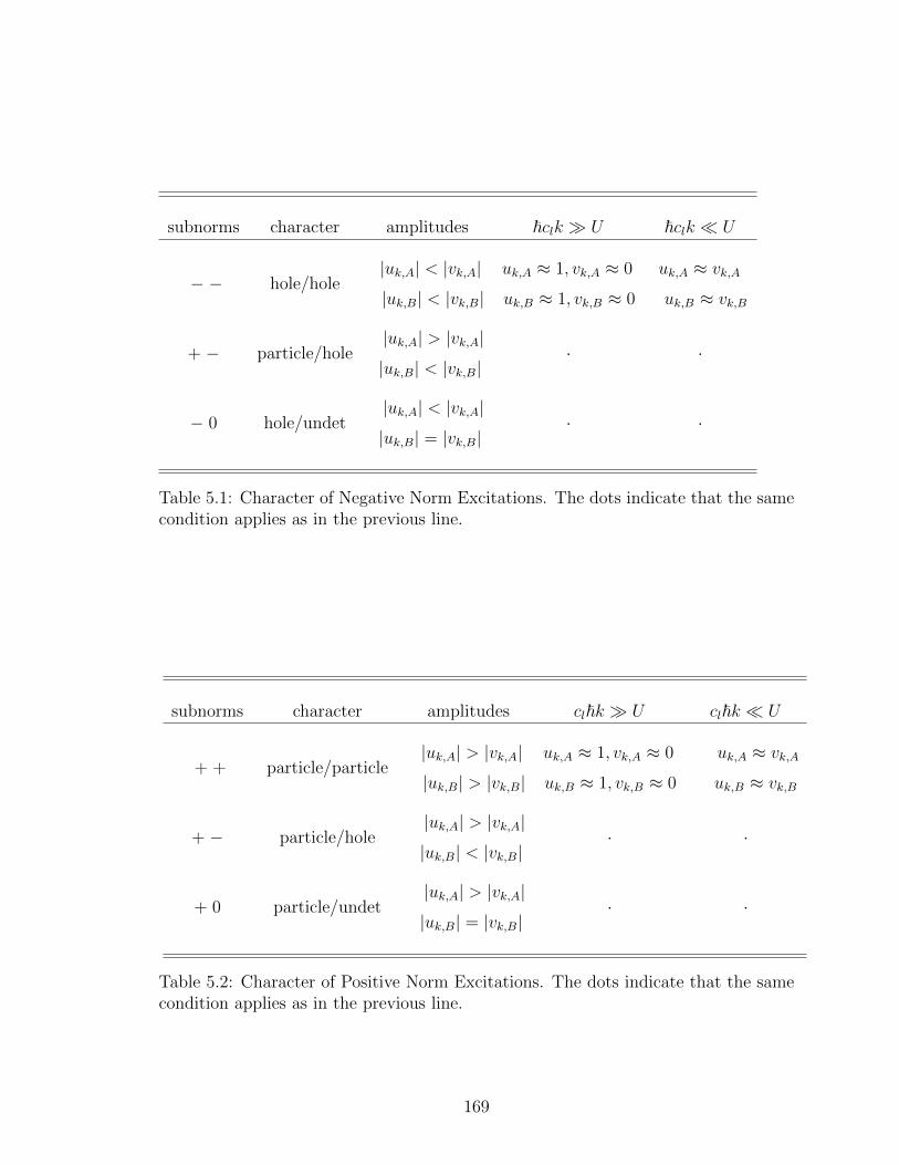
subnorms character amplitudes ~clk U ~clk U

− − hole/hole|uk,A| < |vk,A||uk,B| < |vk,B|

uk,A ≈ 1, vk,A ≈ 0

uk,B ≈ 1, vk,B ≈ 0

uk,A ≈ vk,A

uk,B ≈ vk,B

+ − particle/hole|uk,A| > |vk,A||uk,B| < |vk,B|

· ·

− 0 hole/undet|uk,A| < |vk,A||uk,B| = |vk,B|

· ·

Table 5.1: Character of Negative Norm Excitations. The dots indicate that the samecondition applies as in the previous line.

subnorms character amplitudes cl~k U cl~k U

+ + particle/particle|uk,A| > |vk,A||uk,B| > |vk,B|

uk,A ≈ 1, vk,A ≈ 0

uk,B ≈ 1, vk,B ≈ 0

uk,A ≈ vk,A

uk,B ≈ vk,B

+ − particle/hole|uk,A| > |vk,A||uk,B| < |vk,B|

· ·

+ 0 particle/undet|uk,A| > |vk,A||uk,B| = |vk,B|

· ·

Table 5.2: Character of Positive Norm Excitations. The dots indicate that the samecondition applies as in the previous line.

169

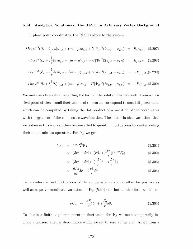
5.14 Analytical Solutions of the RLSE for Arbitrary Vortex Background

In plane polar coordinates, the RLSE reduce to the system

i ~cl e−iθ(∂r − i1

r∂θ)uj,B + (m− µ)uj,A + U |ΨA|2(2uj,A − vj,A) = Ejuj,A , (5.297)

i ~cl eiθ(∂r + i1

r∂θ)uj,A + (m− µ)uj,B + U |Ψb|2(2uj,B − vj,B) = Ejuj,B , (5.298)

i ~cl e−iθ(∂r − i1

r∂θ)vj,B + (m− µ)vj,A + U |ΨA|2(2vj,A − uj,A) = −Ejvj,A ,(5.299)

i ~cl eiθ(∂r + i1

r∂θ)vj,A + (m− µ)vj,B + U |ΨB|2(2vj,B − uj,B) = −Ejvj,B .(5.300)

We make an observation regarding the form of the solution that we seek. From a clas-

sical point of view, small fluctuations of the vortex correspond to small displacements

which can be computed by taking the dot product of a variation of the coordinates

with the gradient of the condensate wavefunction. The small classical variations that

we obtain in this way can then be converted to quantum fluctuations by reinterpreting

their amplitudes as operators. For ΨA we get

δΨA = δ~r · ~∇ΨA (5.301)

∼ (δrr + δθθ) · (r∂r + θ∂θr

)(e−iθF0) (5.302)

∼ (δrr + δθθ) · (dF0

drr − i F0

rθ) (5.303)

∼ dF0

drδr − i F0

rδθ. (5.304)

To reproduce actual fluctuations of the condensate we should allow for positive as

well as negative coordinate variations in Eq. (5.304) so that another form would be

δΨA ∼ dF0

drδr + i

F0

rδθ. (5.305)

To obtain a finite angular momentum fluctuation for ΨB we must temporarily in-

clude a nonzero angular dependence which we set to zero at the end. Apart from a

170

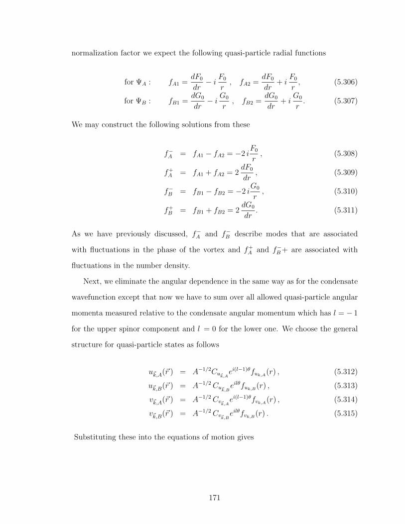
normalization factor we expect the following quasi-particle radial functions

for ΨA : fA1 =dF0

dr− i F0

r, fA2 =

dF0

dr+ i

F0

r, (5.306)

for ΨB : fB1 =dG0

dr− i G0

r, fB2 =

dG0

dr+ i

G0

r. (5.307)

We may construct the following solutions from these

f−A = fA1 − fA2 = −2 iF0

r, (5.308)

f+A = fA1 + fA2 = 2

dF0

dr, (5.309)

f−B = fB1 − fB2 = −2 iG0

r, (5.310)

f+B = fB1 + fB2 = 2

dG0

dr. (5.311)

As we have previously discussed, f−A and f−B describe modes that are associated

with fluctuations in the phase of the vortex and f+A and f−B+ are associated with

fluctuations in the number density.

Next, we eliminate the angular dependence in the same way as for the condensate

wavefunction except that now we have to sum over all allowed quasi-particle angular

momenta measured relative to the condensate angular momentum which has l = − 1

for the upper spinor component and l = 0 for the lower one. We choose the general

structure for quasi-particle states as follows

u~k,A(~r ) = A−1/2Cu~k,Aei(l−1)θfuk,A(r) , (5.312)

u~k,B(~r ) = A−1/2Cu~k,Beilθfuk,B(r) , (5.313)

v~k,A(~r ) = A−1/2Cv~k,Aei(l−1)θfvk,A(r) , (5.314)

v~k,B(~r ) = A−1/2Cv~k,Beilθfvk,B(r) . (5.315)

Substituting these into the equations of motion gives

171

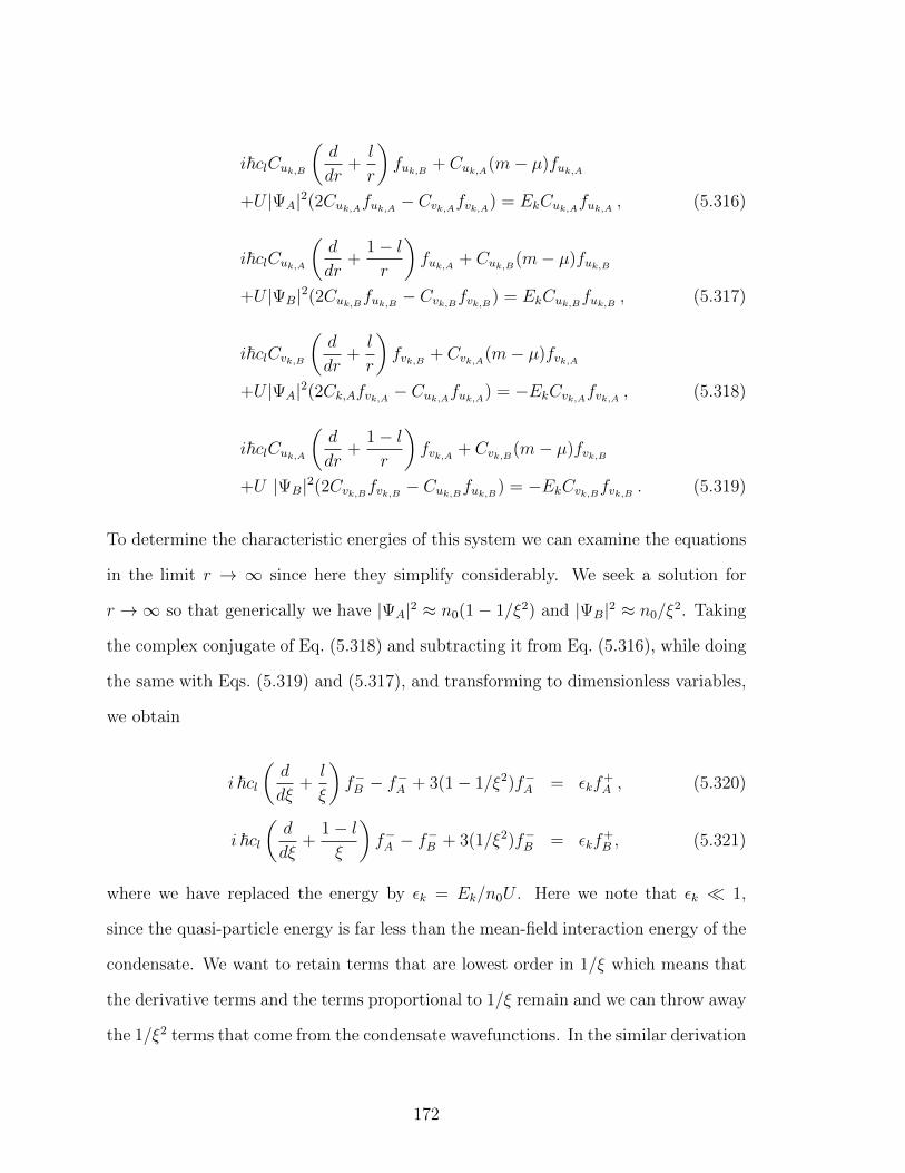
i~clCuk,B

(d

dr+l

r

)fuk,B + Cuk,A(m− µ)fuk,A

+U |ΨA|2(2Cuk,Afuk,A − Cvk,Afvk,A) = EkCuk,Afuk,A , (5.316)

i~clCuk,A

(d

dr+

1− lr

)fuk,A + Cuk,B(m− µ)fuk,B

+U |ΨB|2(2Cuk,Bfuk,B − Cvk,Bfvk,B) = EkCuk,Bfuk,B , (5.317)

i~clCvk,B

(d

dr+l

r

)fvk,B + Cvk,A(m− µ)fvk,A

+U |ΨA|2(2Ck,Afvk,A − Cuk,Afuk,A) = −EkCvk,Afvk,A , (5.318)

i~clCuk,A

(d

dr+

1− lr

)fvk,A + Cvk,B(m− µ)fvk,B

+U |ΨB|2(2Cvk,Bfvk,B − Cuk,Bfuk,B) = −EkCvk,Bfvk,B . (5.319)

To determine the characteristic energies of this system we can examine the equations

in the limit r → ∞ since here they simplify considerably. We seek a solution for

r →∞ so that generically we have |ΨA|2 ≈ n0(1− 1/ξ2) and |ΨB|2 ≈ n0/ξ2. Taking

the complex conjugate of Eq. (5.318) and subtracting it from Eq. (5.316), while doing

the same with Eqs. (5.319) and (5.317), and transforming to dimensionless variables,

we obtain

i ~cl(d

dξ+l

ξ

)f−B − f−A + 3(1− 1/ξ2)f−A = εkf

+A , (5.320)

i ~cl(d

dξ+

1− lξ

)f−A − f−B + 3(1/ξ2)f−B = εkf

+B , (5.321)

where we have replaced the energy by εk = Ek/n0U . Here we note that εk 1,

since the quasi-particle energy is far less than the mean-field interaction energy of the

condensate. We want to retain terms that are lowest order in 1/ξ which means that

the derivative terms and the terms proportional to 1/ξ remain and we can throw away

the 1/ξ2 terms that come from the condensate wavefunctions. In the similar derivation

172

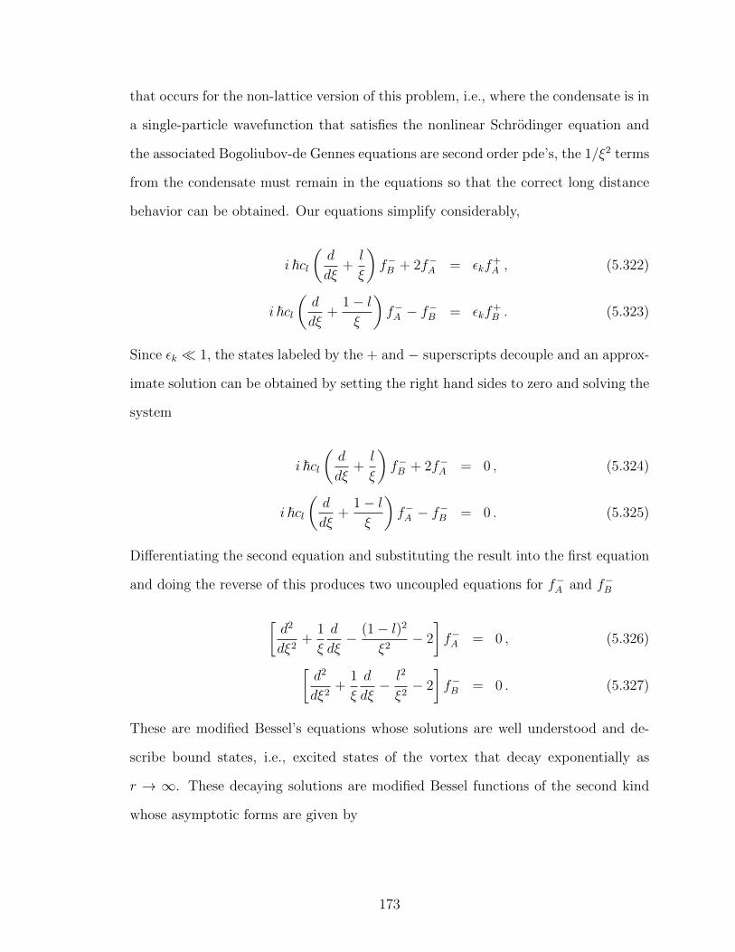
that occurs for the non-lattice version of this problem, i.e., where the condensate is in

a single-particle wavefunction that satisfies the nonlinear Schrodinger equation and

the associated Bogoliubov-de Gennes equations are second order pde’s, the 1/ξ2 terms

from the condensate must remain in the equations so that the correct long distance

behavior can be obtained. Our equations simplify considerably,

i ~cl(d

dξ+l

ξ

)f−B + 2f−A = εkf

+A , (5.322)

i ~cl(d

dξ+

1− lξ

)f−A − f−B = εkf

+B . (5.323)

Since εk 1, the states labeled by the + and − superscripts decouple and an approx-

imate solution can be obtained by setting the right hand sides to zero and solving the

system

i ~cl(d

dξ+l

ξ

)f−B + 2f−A = 0 , (5.324)

i ~cl(d

dξ+

1− lξ

)f−A − f−B = 0 . (5.325)

Differentiating the second equation and substituting the result into the first equation

and doing the reverse of this produces two uncoupled equations for f−A and f−B

[d2

dξ2+

1

ξ

d

dξ− (1− l)2

ξ2− 2

]f−A = 0 , (5.326)[

d2

dξ2+

1

ξ

d

dξ− l2

ξ2− 2

]f−B = 0 . (5.327)

These are modified Bessel’s equations whose solutions are well understood and de-

scribe bound states, i.e., excited states of the vortex that decay exponentially as

r → ∞. These decaying solutions are modified Bessel functions of the second kind

whose asymptotic forms are given by

173

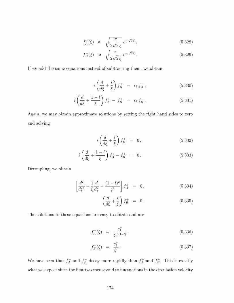
f−A (ξ) ≈√

π

2√

2 ξe−√

2 ξ , (5.328)

f−B (ξ) ≈√

π

2√

2 ξe−√

2 ξ . (5.329)

If we add the same equations instead of subtracting them, we obtain

i

(d

dξ+l

ξ

)f+B = εk f

−A , (5.330)

i

(d

dξ+

1− lξ

)f+A − f+

B = εk f−B . (5.331)

Again, we may obtain approximate solutions by setting the right hand sides to zero

and solving

i

(d

dξ+l

ξ

)f+B = 0 , (5.332)

i

(d

dξ+

1− lξ

)f+A − f+

B = 0 . (5.333)

Decoupling, we obtain

[d2

dξ2+

1

ξ

d

dξ− (1− l)2

ξ2

]f+A = 0 , (5.334)(

d

dξ+l

ξ

)f+B = 0 . (5.335)

The solutions to these equations are easy to obtain and are

f+A (ξ) =

c+1

ξ±(1−l) , (5.336)

f+B (ξ) =

c+2

ξl. (5.337)

We have seen that f−A and f−B decay more rapidly than f+A and f+

B . This is exactly

what we expect since the first two correspond to fluctuations in the circulation velocity

174

potential of the vortex while the last two correspond to fluctuations in the number

density which are expected to fall off more slowly.

5.15 Conclusion

In this chapter, we have derived the RLSE and applied them to the case of a

uniform BEC. and compute the coherence factors for the uniform case to obtain the

coherence factors, energy eigenvalues and studied their limiting forms as a function of

the quasi-partcle momentum relative to the natural parameters of the system, i.e., the

particle interaction, lattice spacing, and hopping energy. Moreover, we have shed light

on the normalization of positive and negative energy quasi-particle states, including

symmetries of the RLSE, and delineated the different types of spinor excitations where

we have seen how the particle-hole picture for ordinary weakly interacting BECs is

another dimensional scale to the Dirac particle-antiparticle paradigm familiar from

studies of graphene. The interacting, metastable, ground state energy was determined

with corrections beyond the mean field result, and has a clear limit to its counterpart

describing non-interacting bosons in the honeycomb lattice. Finally, we have solved,

by approximate analytical methods, the RLSE for the case of vortex, and interpret

our results by analogy with the semiclassical picture that small fluctuations of the

vortex are equivalent to fluctuations in its shape and spatial position, i.e., fluctuations

in the location of the core and the phase angle. We obtain decaying and non-decaying

solutions, where the former correspond to bound state fluctuations of the vortex and

the latter are free-scattering states.

175

CHAPTER 6

THE NONLINEAR DIRAC EQUATION: RELATIVISTIC VORTICES AND

EXPERIMENTAL REALIZATION IN BOSE-EINSTEIN CONDENSATES

L. H. Haddad, K. M. O’Hara, and Lincoln D. Carr, Physical Review

Letters, under review, 2012.

Abstract

We present a detailed experimental procedure for preparing relativistic vortices,

governed by the nonlinear Dirac equation, in a two-dimensional Bose-Einstein con-

densate (BEC) in a honeycomb optical lattice. Our setup contains Dirac points, in

direct analogy to graphene. We determine a range of practical values for all rele-

vant physical parameters needed to realize relativistic vortices in BEC of 87Rb atoms.

Discrete spectra for seven distinct vortices are computed in the presence of a weak

harmonic trap, which include Anderson-Toulouse and Mermin-Ho skyrmion textures,

and half-quantum vortices. We find that most vortices are stable with a lifetime

between 1 and 10 seconds.

177

6.1 Main Text

Multi-component Bose-Einstein condensates (BECs) present an ideal setting for

studying complex vortex structures [44]. Such vortices allow for topologically intrigu-

ing configurations ranging from skyrmions to knots [38, 43, 182]. The usual method

for adding a spinor structure to a BEC relies on hyperfine degrees of freedom or differ-

ent atomic species. Instead, we use the band structure and linear dispersion relation

around the Dirac points at the Brillouin zone edge of a honeycomb optical lattice

to realize a four-component Dirac spinor, in direct analogy to graphene [183]. This

gives us both pseudospin as well as a relativistic structure. To accomplish this, we

propose starting with a BEC of weakly interacting alkali metal atoms in the lowest

Bloch state of a 2D honeycomb optical lattice, then using Bragg scattering to pop-

ulate Bloch states at the two inequivalent Dirac points, followed by the application

of a Laguerre-Gaussian laser beam to deliver a net angular momentum to the BEC

which excites a plethora of vortex structures. The vortices we obtain are solutions

of the nonlinear Dirac equation (NLDE), whose stability is determined by the rela-

tivistic linear stability equations (RLSE) [52, 184]. Our work on the NLDE+RLSE

system opens up the field of relativistic simulations in BECs at velocities ten orders

of magnitude slower than the speed of light.

In this letter we combine the study of Dirac points with superfluid vortices, an

environment reminiscent of particle physics models where relativistic vortices are com-

monplace [185, 186]. Stability of a BEC at the Dirac points presents a challenge, since

Bloch states there have finite crystal momentum and nonzero energy. We handle this

problem by introducing an intermediate asymmetry between the A and B sublattice

potential depths which opens up a mass gap. Using a gap enables us to construct

initial and final Bloch states, ψA,0 and ψA,K (with Dirac point momentum K), as

superpositions of the two degenerate states at the Dirac point with velocities cl and

−cl, respectively. This produces a state with group velocity equal to zero, relative to

178

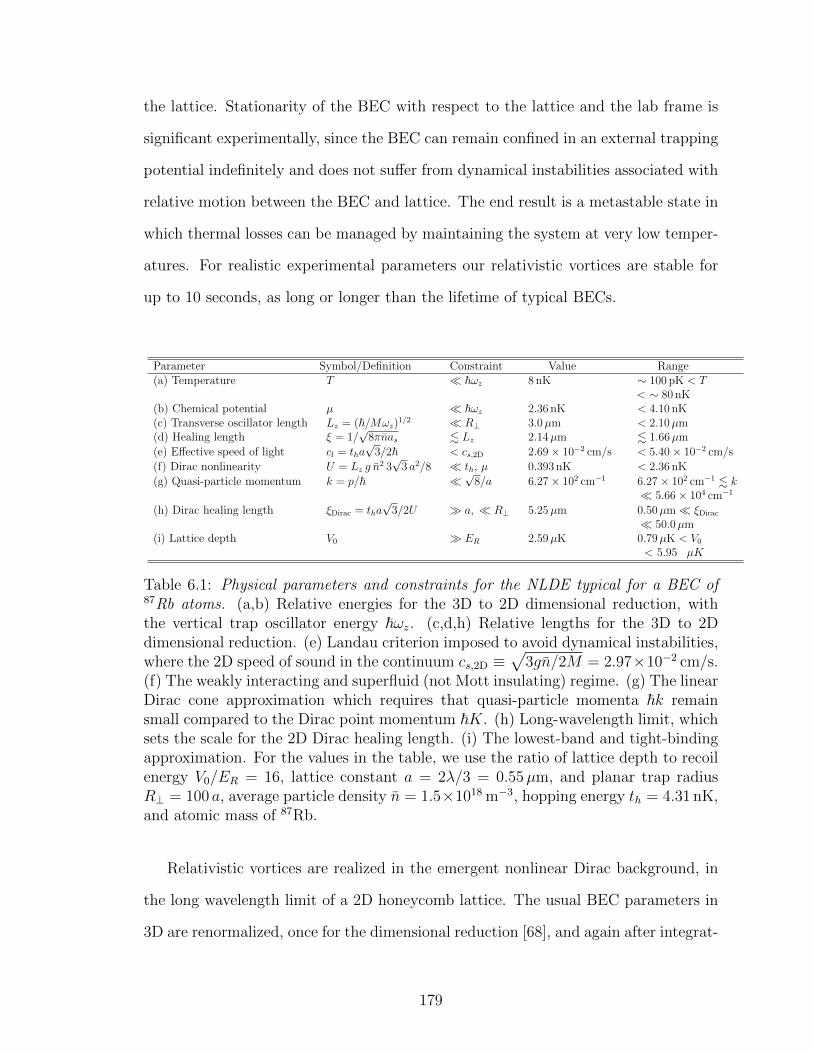
the lattice. Stationarity of the BEC with respect to the lattice and the lab frame is

significant experimentally, since the BEC can remain confined in an external trapping

potential indefinitely and does not suffer from dynamical instabilities associated with

relative motion between the BEC and lattice. The end result is a metastable state in

which thermal losses can be managed by maintaining the system at very low temper-

atures. For realistic experimental parameters our relativistic vortices are stable for

up to 10 seconds, as long or longer than the lifetime of typical BECs.

Parameter Symbol/Definition Constraint Value Range(a) Temperature T ~ωz 8 nK ∼ 100 pK < T

< ∼ 80 nK(b) Chemical potential µ ~ωz 2.36 nK < 4.10 nK(c) Transverse oscillator length Lz = (~/Mωz)

1/2 R⊥ 3.0µm < 2.10µm(d) Healing length ξ = 1/

√8πnas . Lz 2.14µm . 1.66µm

(e) Effective speed of light cl = tha√

3/2~ < cs,2D 2.69× 10−2 cm/s < 5.40× 10−2 cm/s

(f) Dirac nonlinearity U = Lz g n2 3√

3 a2/8 th, µ 0.393 nK < 2.36 nK

(g) Quasi-particle momentum k = p/~ √

8/a 6.27× 102 cm−1 6.27× 102 cm−1 . k 5.66× 104 cm−1

(h) Dirac healing length ξDirac = tha√

3/2U a, R⊥ 5.25µm 0.50µm ξDirac

50.0µm(i) Lattice depth V0 ER 2.59µK 0.79µK < V0

< 5.95 µK

Table 6.1: Physical parameters and constraints for the NLDE typical for a BEC of87Rb atoms. (a,b) Relative energies for the 3D to 2D dimensional reduction, withthe vertical trap oscillator energy ~ωz. (c,d,h) Relative lengths for the 3D to 2Ddimensional reduction. (e) Landau criterion imposed to avoid dynamical instabilities,where the 2D speed of sound in the continuum cs,2D ≡

√3gn/2M = 2.97×10−2 cm/s.

(f) The weakly interacting and superfluid (not Mott insulating) regime. (g) The linearDirac cone approximation which requires that quasi-particle momenta ~k remainsmall compared to the Dirac point momentum ~K. (h) Long-wavelength limit, whichsets the scale for the 2D Dirac healing length. (i) The lowest-band and tight-bindingapproximation. For the values in the table, we use the ratio of lattice depth to recoilenergy V0/ER = 16, lattice constant a = 2λ/3 = 0.55µm, and planar trap radiusR⊥ = 100 a, average particle density n = 1.5×1018 m−3, hopping energy th = 4.31 nK,and atomic mass of 87Rb.

Relativistic vortices are realized in the emergent nonlinear Dirac background, in

the long wavelength limit of a 2D honeycomb lattice. The usual BEC parameters in

3D are renormalized, once for the dimensional reduction [68], and again after integrat-

179

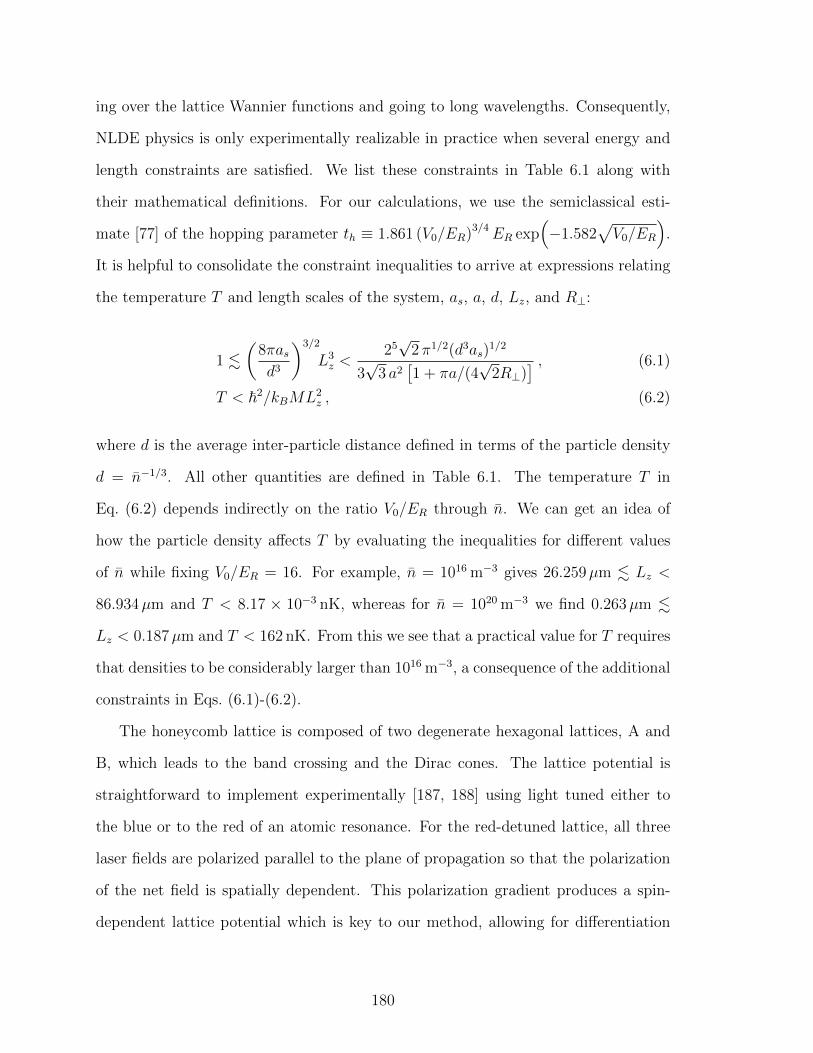
ing over the lattice Wannier functions and going to long wavelengths. Consequently,

NLDE physics is only experimentally realizable in practice when several energy and

length constraints are satisfied. We list these constraints in Table 6.1 along with

their mathematical definitions. For our calculations, we use the semiclassical esti-

mate [77] of the hopping parameter th ≡ 1.861 (V0/ER)3/4ER exp(−1.582

√V0/ER

).

It is helpful to consolidate the constraint inequalities to arrive at expressions relating

the temperature T and length scales of the system, as, a, d, Lz, and R⊥:

1 .

(8πasd3

)3/2

L3z <

25√

2 π1/2(d3as)1/2

3√

3 a2[1 + πa/(4

√2R⊥)

] , (6.1)

T < ~2/kBML2z , (6.2)

where d is the average inter-particle distance defined in terms of the particle density

d = n−1/3. All other quantities are defined in Table 6.1. The temperature T in

Eq. (6.2) depends indirectly on the ratio V0/ER through n. We can get an idea of

how the particle density affects T by evaluating the inequalities for different values

of n while fixing V0/ER = 16. For example, n = 1016 m−3 gives 26.259µm . Lz <

86.934µm and T < 8.17 × 10−3 nK, whereas for n = 1020 m−3 we find 0.263µm .

Lz < 0.187µm and T < 162 nK. From this we see that a practical value for T requires

that densities to be considerably larger than 1016 m−3, a consequence of the additional

constraints in Eqs. (6.1)-(6.2).

The honeycomb lattice is composed of two degenerate hexagonal lattices, A and

B, which leads to the band crossing and the Dirac cones. The lattice potential is

straightforward to implement experimentally [187, 188] using light tuned either to

the blue or to the red of an atomic resonance. For the red-detuned lattice, all three

laser fields are polarized parallel to the plane of propagation so that the polarization

of the net field is spatially dependent. This polarization gradient produces a spin-

dependent lattice potential which is key to our method, allowing for differentiation

180

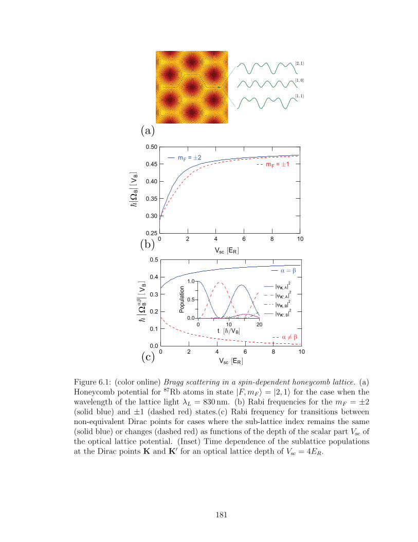
Vsc [ER ]

m = §2

[ VB]

¹h Ω

F

m = §1F

j

j B

j1; 0i

j1; 1i

j2; 1i

Vsc [ER ]

t [¹h=VB]

Population

α = β

α = β

1.0

0.0

0.5

0 10 20

[ VB]

¹h Ωj

j

B

0.5

0.4

0.3

0.2

0.1

0.0

α,β

(a)

(b)

(c)

Figure 6.1: (color online) Bragg scattering in a spin-dependent honeycomb lattice. (a)Honeycomb potential for 87Rb atoms in state |F,mF 〉 = |2, 1〉 for the case when thewavelength of the lattice light λL = 830 nm. (b) Rabi frequencies for the mF = ±2(solid blue) and ±1 (dashed red) states.(c) Rabi frequency for transitions betweennon-equivalent Dirac points for cases where the sub-lattice index remains the same(solid blue) or changes (dashed red) as functions of the depth of the scalar part Vsc ofthe optical lattice potential. (Inset) Time dependence of the sublattice populationsat the Dirac points K and K′ for an optical lattice depth of Vsc = 4ER.

181

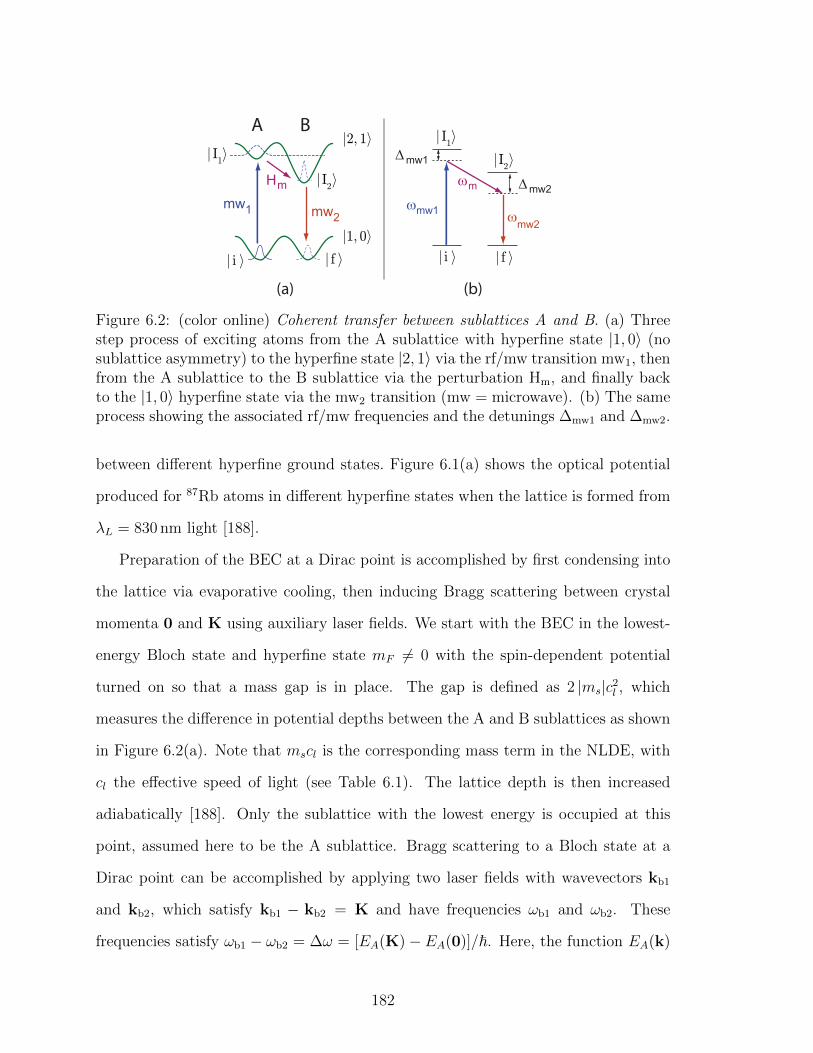
j2; 1iBA

j1; 0i

mw1 mw

2

Hm

ωmw1

ωmw2

ωm

∆mw1

∆mw2

j i i j f i

j I1i

jI2i

j i i j f i

j I1i

jI2i

(a) (b)

Figure 6.2: (color online) Coherent transfer between sublattices A and B. (a) Threestep process of exciting atoms from the A sublattice with hyperfine state |1, 0〉 (nosublattice asymmetry) to the hyperfine state |2, 1〉 via the rf/mw transition mw1, thenfrom the A sublattice to the B sublattice via the perturbation Hm, and finally backto the |1, 0〉 hyperfine state via the mw2 transition (mw = microwave). (b) The sameprocess showing the associated rf/mw frequencies and the detunings ∆mw1 and ∆mw2.

between different hyperfine ground states. Figure 6.1(a) shows the optical potential

produced for 87Rb atoms in different hyperfine states when the lattice is formed from

λL = 830 nm light [188].

Preparation of the BEC at a Dirac point is accomplished by first condensing into

the lattice via evaporative cooling, then inducing Bragg scattering between crystal

momenta 0 and K using auxiliary laser fields. We start with the BEC in the lowest-

energy Bloch state and hyperfine state mF 6= 0 with the spin-dependent potential

turned on so that a mass gap is in place. The gap is defined as 2 |ms|c2l , which

measures the difference in potential depths between the A and B sublattices as shown

in Figure 6.2(a). Note that mscl is the corresponding mass term in the NLDE, with

cl the effective speed of light (see Table 6.1). The lattice depth is then increased

adiabatically [188]. Only the sublattice with the lowest energy is occupied at this

point, assumed here to be the A sublattice. Bragg scattering to a Bloch state at a

Dirac point can be accomplished by applying two laser fields with wavevectors kb1

and kb2, which satisfy kb1 − kb2 = K and have frequencies ωb1 and ωb2. These

frequencies satisfy ωb1 − ωb2 = ∆ω = [EA(K)− EA(0)]/~. Here, the function EA(k)

182

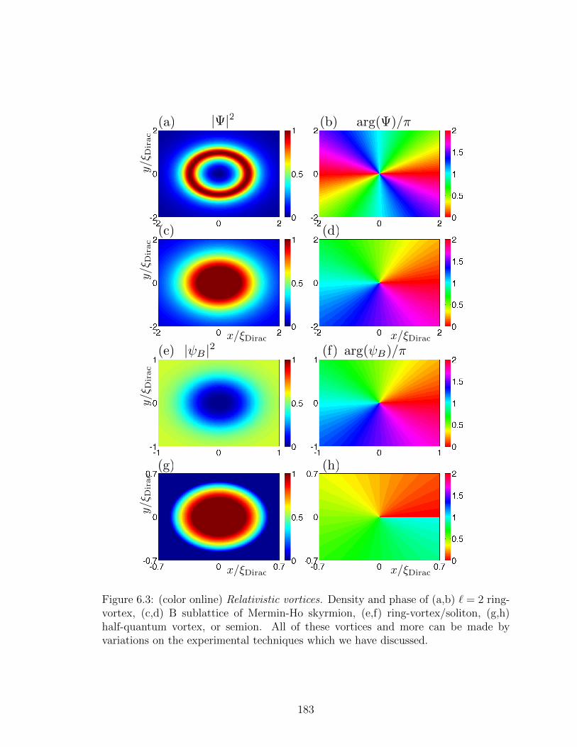
x/ξDiracx/ξDirac

y/ξ

Dirac

y/ξ

Dirac

|Ψ|2 arg(Ψ)/π(a) (b)

x/ξDiracx/ξDirac

y/ξ

Dirac

y/ξ

Dirac

|ψB |2 arg(ψB)/π

(c) (d)

(g) (h)

(e) (f)

Figure 6.3: (color online) Relativistic vortices. Density and phase of (a,b) ` = 2 ring-vortex, (c,d) B sublattice of Mermin-Ho skyrmion, (e,f) ring-vortex/soliton, (g,h)half-quantum vortex, or semion. All of these vortices and more can be made byvariations on the experimental techniques which we have discussed.

183

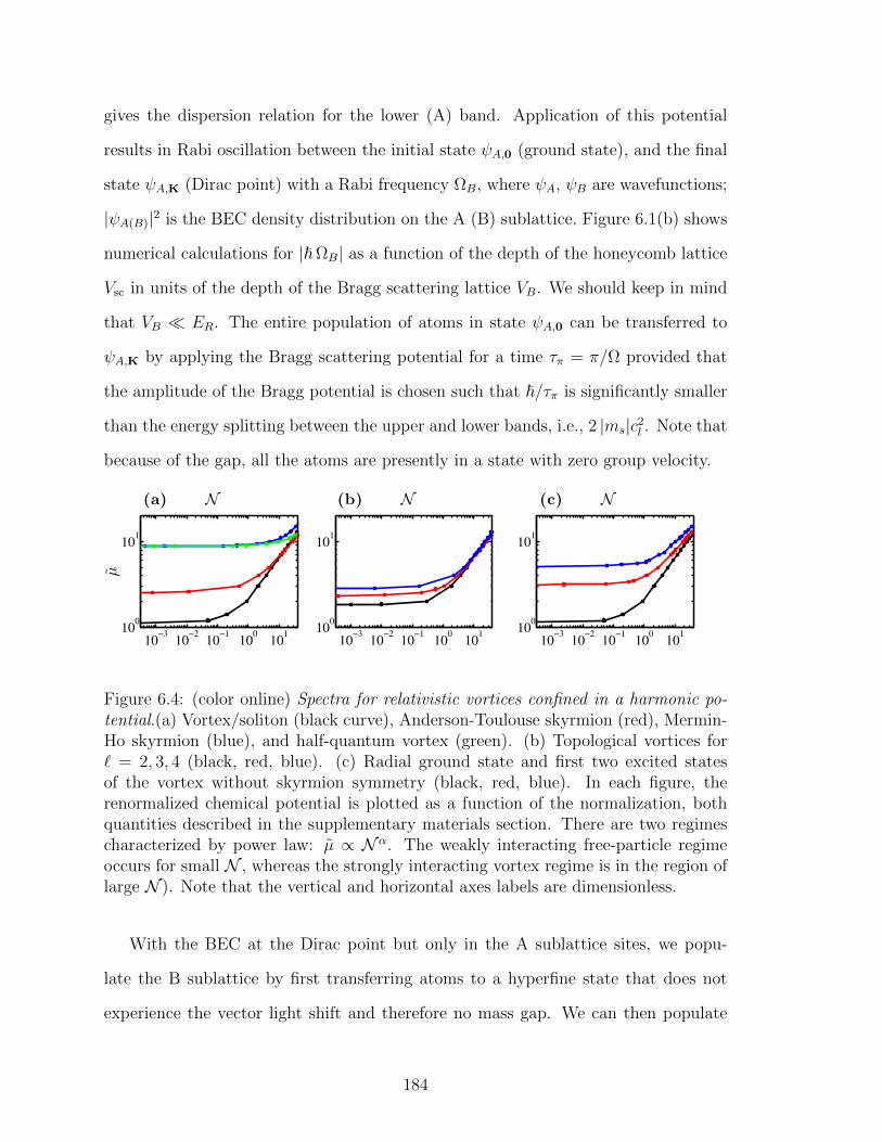
gives the dispersion relation for the lower (A) band. Application of this potential

results in Rabi oscillation between the initial state ψA,0 (ground state), and the final

state ψA,K (Dirac point) with a Rabi frequency ΩB, where ψA, ψB are wavefunctions;

|ψA(B)|2 is the BEC density distribution on the A (B) sublattice. Figure 6.1(b) shows

numerical calculations for |~ΩB| as a function of the depth of the honeycomb lattice

Vsc in units of the depth of the Bragg scattering lattice VB. We should keep in mind

that VB ER. The entire population of atoms in state ψA,0 can be transferred to

ψA,K by applying the Bragg scattering potential for a time τπ = π/Ω provided that

the amplitude of the Bragg potential is chosen such that ~/τπ is significantly smaller

than the energy splitting between the upper and lower bands, i.e., 2 |ms|c2l . Note that

because of the gap, all the atoms are presently in a state with zero group velocity.

10−3

10−2

10−1

100

101

100

101

(a) N

µ

10−3

10−2

10−1

100

101

100

101

(b) N

10−3

10−2

10−1

100

101

100

101

(c) N

Figure 6.4: (color online) Spectra for relativistic vortices confined in a harmonic po-tential.(a) Vortex/soliton (black curve), Anderson-Toulouse skyrmion (red), Mermin-Ho skyrmion (blue), and half-quantum vortex (green). (b) Topological vortices for` = 2, 3, 4 (black, red, blue). (c) Radial ground state and first two excited statesof the vortex without skyrmion symmetry (black, red, blue). In each figure, therenormalized chemical potential is plotted as a function of the normalization, bothquantities described in the supplementary materials section. There are two regimescharacterized by power law: µ ∝ N α. The weakly interacting free-particle regimeoccurs for small N , whereas the strongly interacting vortex regime is in the region oflarge N ). Note that the vertical and horizontal axes labels are dimensionless.

With the BEC at the Dirac point but only in the A sublattice sites, we popu-

late the B sublattice by first transferring atoms to a hyperfine state that does not

experience the vector light shift and therefore no mass gap. We can then populate

184

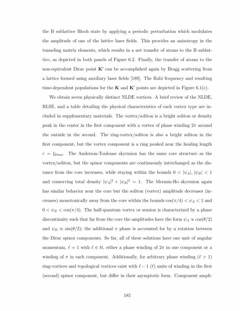
the B sublattice Bloch state by applying a periodic perturbation which modulates

the amplitude of one of the lattice laser fields. This provides an anisotropy in the

tunneling matrix elements, which results in a net transfer of atoms to the B sublat-

tice, as depicted in both panels of Figure 6.2. Finally, the transfer of atoms to the

non-equivalent Dirac point K′ can be accomplished again by Bragg scattering from

a lattice formed using auxiliary laser fields [189]. The Rabi frequency and resulting

time-dependent populations for the K and K′ points are depicted in Figure 6.1(c).

We obtain seven physically distinct NLDE vortices. A brief review of the NLDE,

RLSE, and a table detailing the physical characteristics of each vortex type are in-

cluded in supplementary materials. The vortex/soliton is a bright soliton or density

peak in the center in the first component with a vortex of phase winding 2π around

the outside in the second. The ring-vortex/soliton is also a bright soliton in the

first component, but the vortex component is a ring peaked near the healing length

r = ξDirac. The Anderson-Toulouse skyrmion has the same core structure as the

vortex/soliton, but the spinor components are continuously interchanged as the dis-

tance from the core increases, while staying within the bounds 0 < |ψA|, |ψB| < 1

and conserving total density |ψA|2 + |ψB|2 = 1. The Mermin-Ho skyrmion again

has similar behavior near the core but the soliton (vortex) amplitude decreases (in-

creases) monotonically away from the core within the bounds cos(π/4) < ψA < 1 and

0 < ψB < cos(π/4). The half-quantum vortex or semion is characterized by a phase

discontinuity such that far from the core the amplitudes have the form ψA ∝ cos(θ/2)

and ψB ∝ sin(θ/2); the additional π phase is accounted for by a rotation between

the Dirac spinor components. So far, all of these solutions have one unit of angular

momentum, ` = 1 with ` ∈ N, either a phase winding of 2π in one component or a

winding of π in each component. Additionally, for arbitrary phase winding (` > 1)

ring-vortices and topological vortices exist with `− 1 (`) units of winding in the first

(second) spinor component, but differ in their asymptotic form. Component ampli-

185

tudes for the ring-vortex peak at around one healing length from the core and quickly

decay for large r. On the other hand, topological vortices retain non-zero density far

from the core. Several representative vortices are plotted in Figure 6.3. All of the vor-

tices here can be created using straightforward variations of the transition sequence

depicted in Figure 6.2. In the supplementary materials, we explain how vortices are

realized in practical experiments.

For most of the vortices described in the previous paragraph, we find lifetimes

τ to be long compared to the lifetime of the BEC itself. Using the method which

we present in the supplementary materials section, we obtain the following values

for τ : 9.13 s, 10.43 s, 11.51 s, 1.57×10−7 s, 1.57×10−7 s, 1.25 s, 1.29×10−5 s; for the

vortex/soliton, ring-vortex/soliton, Anderson-Toulouse, Mermin-Ho, half-quantum,

` = 2 ring-vortex, and ` = 2 topological vortex, respectively. To complete our

description, we have computed the discrete spectra pertaining to the case of planar

confinement by a weak harmonic trap. These are plotted in Figure 6.4. Note that

ring-vortices are minimally affected by the presence of a weak trap, since they are

highly localized objects and lie very near the center of the trap.

In conclusion, we have described in detail a method for constructing a stable BEC

at the Dirac points of a honeycomb optical lattice. Our system allows for relativistic

vortex excitations in a macroscopic Dirac spinor wavefunction, providing a means

of studying high energy field theoretic vortices in a condensed matter setting. We

have completely specified the required physical parameters, lifetimes, and spectra for

harmonically bound vortices as a prescription guide for the experimentalist. Varia-

tions on the NLDE have tremendous potential for a host of relativistic simulations in

BECs. Interesting examples include Soler models [190] and the extended Gross-Neveu

model [126]. Our work puts such efforts on a solid experimental footing.

Acknowledgments

186

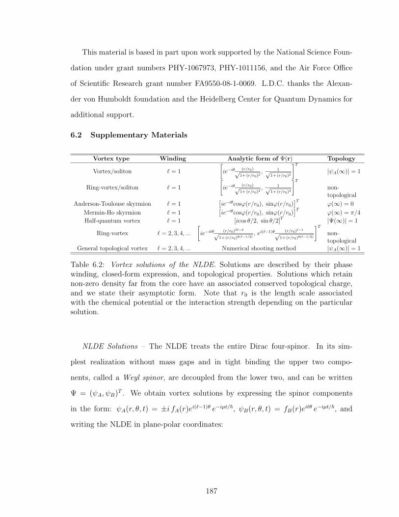
This material is based in part upon work supported by the National Science Foun-

dation under grant numbers PHY-1067973, PHY-1011156, and the Air Force Office

of Scientific Research grant number FA9550-08-1-0069. L.D.C. thanks the Alexan-

der von Humboldt foundation and the Heidelberg Center for Quantum Dynamics for

additional support.

6.2 Supplementary Materials

Vortex type Winding Analytic form of Ψ(r) Topology

Vortex/soliton ` = 1

[ie−iθ (r/r0)√

1+ (r/r0)2, 1√

1+ (r/r0)2

]T|ψA(∞)| = 1

Ring-vortex/soliton ` = 1

[ie−iθ (r/r0)√

1+ (r/r0)4, 1√

1+ (r/r0)4

]Tnon-topological

Anderson-Toulouse skyrmion ` = 1[ie−iθcosϕ(r/r0), sinϕ(r/r0)

]Tϕ(∞) = 0

Mermin-Ho skyrmion ` = 1[ie−iθcosϕ(r/r0), sinϕ(r/r0)

]Tϕ(∞) = π/4

Half-quantum vortex ` = 1 [icos θ/2, sin θ/2]T |Ψ(∞)| = 1

Ring-vortex ` = 2, 3, 4, ...

[ie−i`θ (r/r0)3`−2√

1+ (r/r0)8(`−1/2), ei(`−1)θ (r/r0)`−1√

1+ (r/r0)8(`−1/2)

]Tnon-topological

General topological vortex ` = 2, 3, 4, ... Numerical shooting method |ψA(∞)| = 1

Table 6.2: Vortex solutions of the NLDE. Solutions are described by their phasewinding, closed-form expression, and topological properties. Solutions which retainnon-zero density far from the core have an associated conserved topological charge,and we state their asymptotic form. Note that r0 is the length scale associatedwith the chemical potential or the interaction strength depending on the particularsolution.

NLDE Solutions – The NLDE treats the entire Dirac four-spinor. In its sim-

plest realization without mass gaps and in tight binding the upper two compo-

nents, called a Weyl spinor, are decoupled from the lower two, and can be written

Ψ = (ψA, ψB)T . We obtain vortex solutions by expressing the spinor components

in the form: ψA(r, θ, t) = ±i fA(r)ei(`−1)θ e−iµt/~, ψB(r, θ, t) = fB(r)ei`θ e−iµt/~, and

writing the NLDE in plane-polar coordinates:

187

−~cl(∂r +

`

r

)fB(r) + U |fA(r)|2fA(r) = µfA(r) (6.3)

~cl(∂r +

1−`r

)fA(r) + U |fB(r)|2fB(r) = µfB(r), (6.4)

where ` is the integer phase winding and the other parameters are defined in Ta-

ble 6.1. For the case µ = 0, Eqs. (8.6)-(8.7) give closed form expressions for the

radial amplitudes fA and fB. These are the ring-vortex/soliton (` = 1) and general

ring-vortex (` > 1) solutions. For the case µ 6= 0, closed form solutions exist in some

cases while others are obtained using a numerical shooting method. Solutions of the

NLDE are listed in Table 6.2.

Experimental Realization of Vortices – Relativistic vortices can be excited by

starting with all the atoms in the A sublattice at the Dirac point, then applying

co-propagating Gaussian and Laguerre-Gaussian laser beams, where the Laguerre-

Gaussian beam carries a single unit of orbital angular momentum. The transfer of

angular momentum to the atoms occurs via the stimulated Raman transition [191].

The spatial variation of the beam results in mainly the B sublattice being populated

(the vortex) throughout most of the 2D lattice, except within a small disk which

becomes the core of the vortex. On the other hand, the A sublattice is left depleted

everywhere (the soliton) except near the core of the vortex. This describes excitation

of the vortex/soliton or Anderson-Toulouse skyrmion [184]. The Mermin-Ho vortex

can be obtained by the same process, but by only partially transferring atoms to the

B sublattice. The sublattice amplitudes far from the vortex core are tuned to satisfy

|ψB|2 = |ψA|2 < 1, where |ψA(B)|2 is the density of the BEC in the first (second)

four-spinor component in the NLDE, and vA(B) = ~/M∇φA(B) is the associated rel-

ativistic fluid velocity, with φA(B) = Arg(ψA(B)) the phase, as depicted in Figure 6.3.

The half-quantum vortex or semion can be excited by using a fractional optical vortex

beam in order to provide the required angular phase jump [192, 193]. General topo-

188

logical vortices have phase winding ` > 1, non-zero chemical potential µ, and satisfy

|ψA|, |ψB| 6= 0 far from the center of the trap. These can be created by first rotating

the lattice to excite the desired `−1 state in the A sublattice, then following up with

the Laguerre-Gaussian transition to produce the correct ` versus ` − 1 winding dif-

ferential in the spinor components. We note that there is an alternative approach to

the rotating lattice method. General topological vortex excitations may be induced

by subsequent applications of a two-photon transition with co-propagating Laguerre-

Gaussian/Gaussian beams which transfer the condensate between m = 0 states, i.e.,

from F = 1, m = 0 to F = 2, m = 0 or vice versa. Each two-photon transition would

change the orbital angular momentum of both the A and B sublattices by the orbital

angular momentum carried by the Laguerre-Gaussian beams, while maintaining the

desired winding differential between the A and B sublattices. Finally, ring-vortices

characterized by µ = 0 and |ψA|, |ψB| = 0 far from the center of the trap, can be

obtained from the other vortices by inducing depletion of the BEC from the outer

edge of the trap towards the core. Plots for several vortices are shown in Figure 6.3

with more details regarding solutions of the NLDE discussed in Ref. [184].

RLSE Solutions – The RLSE form a relativistic generalization of the Bogoliubov-

de Gennes equations analogous to the relationship between the NLDE and nonlinear

Schrodinger equation. Thus, in the RLSE the quasi-particle amplitudes u and v are

each vector in form, to match the four-spinor (two-spinor at one Dirac point) they

perturb from. The RLSE can be expressed in 2× 2 matrix-vector form:

Duk − UΨvk = Ekuk, (6.5)

D∗vk − UΨuk = −Ekvk , (6.6)

where D and Ψ are 2× 2 matrices which contain the first-order derivatives (∂x + i∂y)

and the background BEC components ψA, ψB, and Ek is the 2× 2 eigenvalue matrix.

Note that U is the particle interaction. When broken down, Eqs. (7.116)-(7.117) form

189

a 4× 4 eigenvalue problem in the quasi-particle amplitudes uk,A(B) and vk,A(B) (with

momentum k) associated with particle and hole excitations of the A(B) sublattices

at a Dirac point. Vortices possess cylindrical symmetry so we express Eqs. (7.116)-

(7.117) in plane-polar coordinates, factor the quasi-particle amplitudes into radial and

angular parts, then substitute in the particular solution for ψA(B). We then obtain

a set of first-order coupled ODE’s in the radial coordinate to be solved consistently

for the functions uA(B)(r), vA(B)(r) and the associated eigenvalues. We discretize the

derivatives and functions using a forward-backward average finite-difference scheme,

then solve the resulting discrete matrix eigenvalue problem using a standard numerical

diagonalization method.

Vortex Lifetimes – To compute vortex lifetimes, we solve the RLSE to obtain the

quasi-particle spatial functions and eigenvalues. In general, for vortex solutions of the

NLDE certain eigenvalues and eigenmodes key to understanding the physical motion

correspond to Nambu-Goldstone modes, i.e., anomalous with a small imaginary com-

ponent [175]. When thermal losses are small, it is the imaginary part of the linear

eigenvalues which depletes the BEC. We define the vortex lifetime by computing the

time for depletion to reach a significant fraction of the total fixed number of atoms in

the system, and consider only depletion coming from the mode with the largest imag-

inary term in its eigenvalue. The lifetime is then given by τ = [~/Im(E)] ln (R⊥/I),

expressed in terms of the largest linear eigenvalue E and the planar radius of the BEC

R⊥, in units of the lattice constant a (see Table 6.1). Note also that the spatial integral

I here is specific to each vortex type. For the experimental parameters of Table 6.1,

we find the longest lived solutions to be the vortex/soliton and Anderson-Toulouse

vortex with τ = 11.51 s, compared to the typical lifetime of a 87Rb condensate in an

optical lattice of less than a second [194].

Chemical Potential Spectra – In order to have a clear comparative prediction

for energies involved in creating our vortices, we solve the NLDE using a numerical

190

shooting method in the presence of a weak harmonic trap of frequency ω⊥ = 2π ×

0.0387 Hz along the direction of the lattice. This is the frequency associated with

a planar BEC radius equal to 100 times the lattice constant. In this case vortices

come in radially quantized states. For simplicity, we focus mainly on the lowest

radial excitation. Using a generalization of the method in [195], we have obtained

the dimensionless (renormalized) chemical potential µ ≡ µ/~ω⊥ as a function of the

normalization N =√

3 ~ω⊥NU/3t2h for each vortex type, as shown in Figure 6.4.

Here, N is the number of atoms in the system with the other quantities defined

in Table 6.1.

191

CHAPTER 7

THE NONLINEAR DIRAC EQUATION: METASTABLE RELATIVISTIC

VORTICES IN A BOSE-EINSTEIN CONDENSATE

L. H. Haddad, K. M. O’Hara, and Lincoln D. Carr, Physical Review

A, to be submitted, 2012.

Abstract

We present a detailed study of relativistic vortices for bosons within the mean-

field nonlinear Dirac framework of a honeycomb optical lattice. The combined quasi-

relativistic structure of the Dirac point and s-wave scattering for bosons leads to a

large number of combinations of vortex and soliton solutions in the (2+1)-dimensional

spinor amplitudes, most of which we obtain in analytical form. We present a de-

tailed derivation of these solutions which include skyrmions, half-quantum vortices,

Mermin-Ho and Anderson-Toulouse vortices for vortex winding ` = 1. For ` ≥ 2

we obtain topological as well as non-topological vortices in the form of an asymp-

totic Bessel solution, algebraic closed-form solutions, and using standard numerical

shooting methods. We demonstrate the continuous spectral mapping between the

vortex and free particle limits for all of these solutions. A full derivation of the rela-

tivistic linear stability equations (RLSE) is presented by two independent methods.

We prove that the standard Bogoliubov-de Genne equations (BdGE) and nonlinear

Schrodinger equation (NLSE) are nonrelativistic limits of the RLSE and nonlinear

Dirac equation (NLDE), respectively. The RLSE are necessary to determine the sta-

193

bility of generic nonuniform relativistic mean-field backgrounds. We solve the RLSE

for our localized solutions and find anomalous as well as dynamically unstable modes

in the linear spectrum for most solutions. Using parameters for 87Rb for our vortex

backgrounds, we find the imaginary parts of the linear eigenvalues to be two to three

orders of magnitude smaller than the interaction strength and give vortex lifetimes

∼ 10 s. To realize the nonlinear Dirac structure in the laboratory, we propose using

Bragg scattering to obtain a condensate at the K and K′ points of the reciprocal

lattice, and co-propagating Laguerre-Gaussian and Gaussian laser beams to induce

the two-photon Raman transitions in 87Rb needed to create our vortex solutions.

7.1 Introduction

Vortices and solitons appear in physical settings which span a wide range of energy

scales and disciplines. Well known examples are solitary waves in water, quantized

vortices in 4He, and Bogomol’nyi-Prasad-Sommerfield states in supersymmetric field

theories [196]. Vortices are relevant from a technological standpoint in quantum com-

puting for example [197], as well as in more theoretical areas of research such as

galactic halos in Bose-Einstein condensate theories of dark matter [198]. In Bose-

Einstein condensates (BECs), vortices as stable rotating solutions of the nonlinear

Schrodinger equation (NLSE) are ubiquitous [17, 199]. Indeed, the presence of a

persistent quantized rotation may be considered a defining property of superfluid-

ity. Although a variety of types of vortices are possible in atomic condensates [44],

the Laplacian inherent to the Schrodinger Hamiltonian constrains the number of ob-

servable vortex structures in the BEC. For instance, a BEC made up of spin-F bosons

gives rise to a (2F +1)-component order parameter which nevertheless solves a multi-

component NLSE. An alternative method of constructing a multicomponent BEC is

194

to add the internal degrees of freedom by placing a condensate in a two-dimensional

honeycomb optical lattice. Atoms are condensed into the lowest energy Bloch state

then translated to a corner of the Brillouin zone using laser assisted Bragg scattering.

At wavelengths large compared to the lattice constant, the microscopic details of the

lattice manifest as an additional SL(2,C) spin group symmetry, i.e., a Dirac point

structure emerges [52].

Multicomponent solitons in (2 + 1)-dimensions may be classified as topological if

they are associated with a topologically conserved quantity, otherwise they are deemed

nontopological. Topological solitons may be further labeled by the relevant homotopy

group. In the case of a non-trivial first homotopy group, an overall macroscopic phase

wraps around the circular boundary consisting of radial lengths much larger than

the healing length, while the internal spin degrees of freedom remain topologically

unconstrained. These are simply referred to as vortices and are distinguished by a

nonvanishing radial profile at infinity. In contrast to these, when the wrapping around

the circular boundary includes the internal spin degrees of freedom in a nontrivial way,

the second-homotopy group is the relevant group and the order parameter is called a

vortex texture or skyrmion [44, 200].

In this article, we study relativistic quantum vortices in the superfluid phase of

a Bose gas at the Dirac point of a honeycomb optical lattice. We first provide the

experimental steps for creating relativistic vortices. We then focus heavily on explicit

vortex solutions of the NLDE. We begin with a preliminary asymptotic solution us-

ing Bessel functions, which provides a basic insight into the structure of the NLDE.

Algebraic solutions are then obtained by considering the zero-chemical potential case.

These are characterized by the condition that the derivative and repulsive interac-

tions cancel exactly. However, for the general case of a non-zero chemical potential,

analytical solutions are only possible when one unit of winding is considered; we use a

numerical approach to obtain vortices with arbitrarily large winding number. A com-

195

bination of numerical and analytical techniques yields skyrmion and half-quantum

vortices (texture vortices). Having obtained our solutions, we compute their cor-

responding discrete chemical potential spectra in the presence of a weak harmonic

potential. This gives us the low-temperature µ versus U landscape for relativistic

vortices, where µ and U are the chemical potential and lattice renormalized particle

interaction, respectively. For example, for finite chemical potential µ we find that

a series of phase transitions occur as U is tuned from zero upward: we encounter

a Mermin-Ho skyrmion transitioning into a half-quantum vortex, followed by the

Anderson-Toulouse skyrmion, then finally into a vortex/soliton (a bright soliton at

the core of a singly-wound topological vortex). To compute lifetimes of our solutions,

we derive a relativistic generalization of Bogoliubov’s equations and solve these for

each solution type. Predictably, we find that vortices with low winding are more

stable than those with large winding number.

In high energy physics and cosmology, relativistic vortices appear as cosmic super-

strings [201–203], in foundational studies in string theory such as mirror symmetry of

Calabi-Yau manifolds [204, 205], and in various brane world scenarios [206]. In gen-

eral, vortices are endemic to gauge theories where spontaneous symmetry breaking

occurs. This includes both the Abelian [185, 203] (as with Nielsen-Olesen vortices in

the Abelian Higgs model) as well as the non-Abelian case [207] (non-Abelian Yang-

Mills for example). Supersymmetric field theories which exhibit weak-strong duality

rely fundamentally on the presence of solitons and vortices which provide the natural

degrees of freedom in the dual theory [186, 203].

In a previous paper, we derived a BEC version of the nonlinear Dirac equation

for the case of weak interparticle interactions [52]. This has attracted attention from

diverse fields of research [20, 21, 32, 103, 110, 120, 121, 168, 208–224]. In the present

paper, we solve the NLDE by several methods to obtain a large class of vortex and

skyrmion solutions. Solutions of the NLDE are effectively long wavelength limit

196

lattice envelopes, and so can cover a large number of sites. The healing length in our

effectively 2D system is typically about 10 times the lattice constant, and we require

the healing length to be small compared to the size of the cylindrical container. In

typical experiments, the number of lattice sites is on the order of 100 in a linear

direction, thus our solutions may be described accurately. These solution types differ

by asymptotic conditions on the amplitude for r much greater than the healing length

(far from the core) or r much less than the healing length (deep inside the core), use of

the internal degree of freedom in the spinor structure, and with respect to quantization

of rotation: Weyl spinor components always differ by one unit of rotation.

In our work, the question of condensate and vortex stability arises in two ways.

First, for bosons, the Dirac point is not bounded below so that a solution of the

NLDE is connected to a continuum of lower energy scattering states through which

decay may occur. We address this issue by noting that for a uniform condensate

at the Dirac point the linear eigenvalues are real : positive and negative valued for

excitations above and below the Dirac point, respectively. This means that a uni-

form condensate is dynamically stable. Furthermore, the thermodynamic instability

implied by the negative eigenvalues can be controlled by reducing the number of ther-

mal excitations in the system. This is accomplished by taking the system to be at

very low temperatures (T µ), reducing the number of collisions between conden-

sate and thermal atoms. This eliminates the dominant mechanism for dissipation and

justifies a metastable interpretation of the condensate [225].

Second, relativistic vortices are excited states of the (Dirac point) condensate,

and we expect to encounter stability issues beyond those which arise in the uniform

case. In particular, we find an “internal dissipation” which occurs as a transfer of

energy between the two components of a Weyl spinor. For ordinary spinor BECs, a

similar coupling occurs through the interaction terms in the Hamiltonian, whereas

for relativistic vortices, the interaction only couples spinor components to themselves,

197

while intercomponent coupling occurs through the kinetic term. Our linear stability

analysis reveals anomalous frequencies with small imaginary parts for several vortex

solutions. For these solutions, one spinor component always lags behind the other by

one unit of rotation, and it is the anomalous modes which reduce the rotation of one

component, while increasing rotation of the other. Strictly speaking, these complex

eigenvalues preclude metastability except in an approximate sense. Nevertheless, cal-

culation of lifetimes based on complex frequencies gives values that are long compared

to the life of the condensate.

Our results are organized as follows. In Sec. 7.2 we map out a detailed prescription

for constructing a condensate at opposite Dirac points and creating our vortices in

the laboratory. We also include a thorough analysis of the physical parameters and

constraints used throughout our work. In Sec. 7.3 we solve the NLDE presenting

closed form and numerical solutions with density and phase plots depicting each

solution type. In Sec. 7.3.2 we solve the NLDE numerically for radial excited states in

a harmonic trapping potential and obtain the discrete spectra for all of our solutions.

In Sec. 7.5 we motivate and provide a full derivation of the RLSE by two methods.

In Sec. 7.6 we solve the RLSE and obtain lifetimes for all of our vortex solutions. In

Sec. 7.7 we summarize our results.

7.2 Experimental Realization of the NLDE

In the laboratory, the NLDE is realizable within a region of parameter space

precisely delineated by constraints on particle density, energies, length scales, etc. We

will discuss these parameters in this section. It is natural to relate our parameters to

those in other areas of research, such as nonlinear optics, in which Dirac dynamics

plays an important role. Creating vortex solutions of the NLDE requires several steps

which are not standard to the usual methods for ordinary BEC vortices. For example,

transferring a condensate from the lowest Bloch mode to the state at the Dirac point

with zero group velocity and amplitude exclusively in one sublattice requires a lattice

198

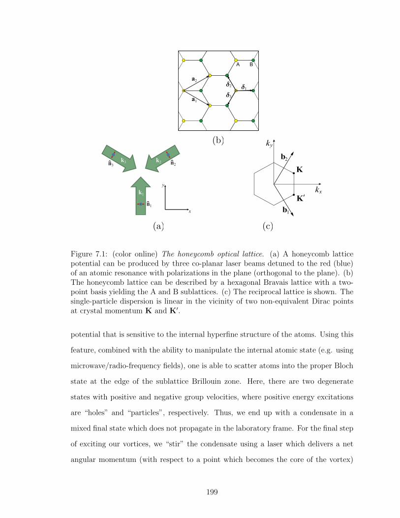
y

x

k2k3

k1

n1

n2n3

b1

b2

K

K‘

kx

ky

(a)

(b)

(c)

a2

a1

A B

2±

3±

1±

Figure 7.1: (color online) The honeycomb optical lattice. (a) A honeycomb latticepotential can be produced by three co-planar laser beams detuned to the red (blue)of an atomic resonance with polarizations in the plane (orthogonal to the plane). (b)The honeycomb lattice can be described by a hexagonal Bravais lattice with a two-point basis yielding the A and B sublattices. (c) The reciprocal lattice is shown. Thesingle-particle dispersion is linear in the vicinity of two non-equivalent Dirac pointsat crystal momentum K and K′.

potential that is sensitive to the internal hyperfine structure of the atoms. Using this

feature, combined with the ability to manipulate the internal atomic state (e.g. using

microwave/radio-frequency fields), one is able to scatter atoms into the proper Bloch

state at the edge of the sublattice Brillouin zone. Here, there are two degenerate

states with positive and negative group velocities, where positive energy excitations

are “holes” and “particles”, respectively. Thus, we end up with a condensate in a

mixed final state which does not propagate in the laboratory frame. For the final step

of exciting our vortices, we “stir” the condensate using a laser which delivers a net

angular momentum (with respect to a point which becomes the core of the vortex)

199

to one or both spinor components.

7.2.1 Renormalized Parameters and Physical Constraints

To obtain the correct renormalized parameters for the NLDE we proceed by two

steps. First, we follow the transformation of the 3D NLSE parameters as we reduce to

the 2D NLSE. Second, we take the long-wavelength limit of the 2D theory at the Dirac

point to get the NLDE, which induces a second renormalization of the parameters.

7.2.2 Transition from 3D to 2D NLSE

A BEC comprised of N atoms of mass M is described by a wavefunction ψ(r, t)

which solves the time-dependent nonlinear Schrodinger equation. The single-particle

density is defined as |ψ(r, t)|2 and the BEC density is defined as ρ(r, t)2 ≡ N |ψ(r, t)|2,

and the phase is φ ≡ arg[ψ(r, t)], with the superfluid velocity given by vs ≡ ∇φ.

The two-particle interaction strength is g = 4π~2as/M and the healing length is

ξ = 1/√

8πnas, where as is the s-wave scattering length for binary collisions between

atoms. We take as > 0 so that g > 0, i.e., we consider only repulsive interactions,

leaving attractive interactions for future studies. Throughout our work, we treat the

case of an axisymmetric system associated with a harmonic trapping potential with

two large dimensions described by a radius R =√x2 + y2, and a small dimension

transverse to the plane described by the length Lz. The average density which appears

in ξ is then defined as n ≡ N/(πR2Lz). Note that ψ(r, t) has dimensions of length−3/2

so that g has dimensions of energy×length3. Another important quantity is the speed

of sound in the condensate, which is defined as cs =√gn/M .

Transforming to the 2D regime requires that as Lz . ξ [73, 226], which ensures

that the condensate remains in the ground state in the transverse direction, and

Lz R, which ensure that excitations along the plane have much lower energy

than those in the transverse direction. The wavefunction can then be separated into

longitudinal and transverse modes, following similar arguments as in Ref. [68],

200

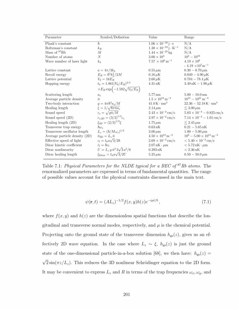
Parameter Symbol/Definition Value Range

Plank’s constant ~ 1.06× 10−34 j · s N/ABoltzman’s constant kB 1.38× 10−23 j ·K−1 N/AMass of 87Rb M 1.44× 10−25 kg N/ANumber of atoms N 3.00× 104 102 − 1010

Wave number of laser light kL 7.57 × 106 m−1 4.19× 106

- 4.19 ×107m−1

Lattice constant a = 4π/3kL 0.55µm 0.30− 0.70µmRecoil energy ER = ~2k2

L/2M 0.16µK 0.049− 4.90µKLattice potential V0 = 16ER 2.60µK 0.784− 78.4µKHopping energy th = 1.861(V0/ER)3/4 4.31 nK 3.49 nK− 1.90µK

×ER exp(−1.582

√V0/ER

)Scattering length as 5.77 nm 5.00− 10.0 nmAverage particle density n 1.5× 1018 m−3 1015 − 1021 m−3

Two-body interaction g = 4π~2as/M 41.0 K · nm3 22.36− 52.18 K · nm3

Healing length ξ = 1/√

8πnas 2.14µm . 3.00µm

Sound speed cs =√gn/M 2.43× 10−2 cm/s 5.83× 10−3 − 0.825 cm/s

Sound speed (2D) cs,2D = (3/2)1/2cs 2.97× 10−2 cm/s 7.14× 10−3 − 1.01 cm/s

Healing length (2D) ξ2D = (2/3)1/2ξ 1.75µm . 2.45µmTransverse trap energy ~ωz 0.63 nK 0.21− 5.65 nKTransverse oscillator length Lz = (~/Mωz)

1/2 3.00µm 1.00− 5.00µmAverage particle density (2D) n2D = Lz n 4.50× 1012 m−2 109 − 5.00× 1015 m−2

Effective speed of light cl = tha√

3/2~ 2.69× 10−2 cm/s < 5.40× 10−2 cm/sDirac kinetic coefficient cl = ~cl 2.07 nK · µm < 5.72 nK · µm

Dirac nonlinearity U = Lz g n2 3√

3 a2/8 0.393 nK < 2.36 nK

Dirac healing length ξDirac = tha√

3/2U 5.25µm 0.50− 50.0µm

Table 7.1: Physical Parameters for the NLDE typical for a BEC of 87Rb atoms. Therenormalized parameters are expressed in terms of fundamental quantities. The rangeof possible values account for the physical constraints discussed in the main text.

ψ(r, t) = (ALz)−1/2f(x, y)h(z)e−iµt/~ , (7.1)

where f(x, y) and h(z) are the dimensionless spatial functions that describe the lon-

gitudinal and transverse normal modes, respectively, and µ is the chemical potential.

Projecting onto the ground state of the transverse dimension hgs(z), gives us an ef-

fectively 2D wave equation. In the case where Lz ∼ ξ, hgs(z) is just the ground

state of the one-dimensional particle-in-a-box solution [68], we then have: hgs(z) =√

2 sin(πz/Lz). This reduces the 3D nonlinear Schrodinger equation to the 2D form.

It may be convenient to express Lz and R in terms of the trap frequencies ωx, ωy, and

201

ωz, in which case we may write: Lz = (~/Mωz)1/2, R =

√~M−1(1/ωx + 1/ωy). The

transformation is then completed by defining the renormalized 2D chemical potential

and interaction as

µ2D ≡ µ+~2π2

2ML2z

, g2D ≡3

2

g

Lz. (7.2)

The 2D renormalized average density can be related to the 3D average density using

the transverse oscillator length or frequency:

n2D ≡N

A= Lz n =

(~

Mωz

)1/2

n . (7.3)

Using this definition and the 2D single-particle wavefunction, ψ(x, y) = A−1/2f(x, y),

we can write the 2D condensate density as ρ2D(x, y) = N |ψ(x, y)|2. The 2D renor-

malized healing length can also be constructed which we find acquires only an extra

numerical factor,

ξ2D ≡(

2

3

)1/21√

8πnas=

(2

3

)1/2

ξ . (7.4)

Similarly, we find the 2D speed of sound to be: cs,2D =√g2Dn2D/M = (3/2)1/2cs. It

is important to keep track of the effect of the reduced dimensionality on the dimen-

sions of the constants: ψ(x, y) now has dimensions of length−1, g2D has dimensions

energy×length2, and n2D has dimensions length−2.

7.2.3 Derivation of NLDE from 2D NLSE.

The derivation of the nonlinear Dirac equation begins with the second quantized

Hamiltonian for a 2D system with the bosonic field operators ψ ≡ ψ(~r, t) = ψ(x, y, t)

obeying bosonic commutation relations in the Heisenberg picture. We then expand

in terms of Bloch states belonging to A or B sites of the honeycomb lattice which

breaks up the bosonic field operator into a sum over the two sublattices. The spatial

202

dependence in this expansion is encapsulated in the exponential Bloch wave and

the Wannier functions w(x, y) which are then integrated out leaving only number-

operator terms in the form of a Dirac-Hubbard Hamiltonian. Finally, the operator

terms are reduced to c-numbers by averaging over on-site coherent states and the

long-wavelength limit is taken. We again recover a continuum theory but with a

Weyl spinor wavefunction Ψ = (ψA, ψB).

7.2.3.1 Normalization Condition.

The key point in discerning the correct normalization (and thus other related quan-

tities) is the contraction of the many-body bosonic operators between localized coher-

ent states. The parameter |ci,j|2 which labels the coherent state at site (i, j), emerges

as the number of atoms at each site, so that ci,j itself becomes the continuous ampli-

tude ψA(r, t) and ψB(r, t) in the long-wavelength limit. Note that the complex moduli

of these amplitudes are pure dimensionless particle numbers, not densities, since they

result from taking the spatial integral over the lattice. With the area per lattice site

given by Al =√

3a2/4, the local time-dependent sublattice densities can be recon-

structed as: ρA(B)(r, t) = |ψA(B)(r, t)|2/Al. Then, the dimensionally correct sublattice

mean-field wavefunctions must be given by ψA(B)(r, t)/√Al = (16/3a4)1/4 ψA(B)(r, t),

where a is the usual lattice spacing. The correct normalization procedure can now be

deduced by writing down the total number of particles in the system

N = (16/3a4)1/2

∫ 2π

0

dφ

∫r dr(|ψA(r, φ; t)|2 + |ψB(r, φ; t)|2), (7.5)

where the upper limit of the radial integral is taken large enough so that the integrand

is negligible. The total number of atoms of the system, N , appears on the right-hand-

side.

203

7.2.3.2 Renormalized Atomic Interaction.

The 3D to 2D reduction and continuum regime result in an effective atomic inter-

action U , a renormalized version of the usual interaction g. We arrive at the explicit

form for U by first approximating the lowest band on-site Wannier functions by the

ground state of the harmonic oscillator potential. Integrating over the area of one

site, we obtain a new local interaction strength:

U ≡ g2D

(√3a2

4

)2

n22D

∫dxdy |wi(x, y)|4

= g2D

(√3a2

4

)2

n22D

(1

2π`2

), (7.6)

where ` is the oscillator length of a lattice potential well. It is often more practical

to express the area of one site in terms of the lattice constant: π`2 =√

3a2/4, and all

other parameters in terms of the corresponding 3D parameters. The interaction then

takes the form

U = Lz g n2 3√

3 a2

8. (7.7)

Note, that U has dimensions of energy.

7.2.3.3 Natural Parameters of the NLDE

We can now identify the main parameters which appear in the NLDE. The di-

mensionful coefficient which multiplies the Dirac kinetic term is the effective speed of

light cl ≈ 0.272 cm/s (compare to the analogous coefficient for relativistic electrons:

c ≈ 3.00×108 m/s). In terms of fundamental constants, we find cl ≡ tha√

3/2~, where

a is the lattice constant and th is the hopping energy. The natural length scale of

the NLDE is the healing length: ξDirac ≡ ~cl/U = tha√

3/2U , which characterizes the

distance over which a disturbance of the condensate will return to its uniform value.

204

We see that ξDirac has the correct dimension of length. To simplify the notation,

for the remainder of our paper we will omit the 2D subscript on all parameters and

assume that these pertain to the 2D NLDE. Finally, the quantity U which appears in

the NLDE determines the strength of the nonlinearity. We have provided a full list

of relevant parameters associated with the NLDE in Table 7.1.

7.2.4 Physical Constraints

The realization of the NLDE in a condensate of 87Rb atoms requires that several

constraints are satisfied which we now list and discuss:

1. Landau Criterion. In order to avoid the instabilities associated with propagation

faster than the sound speed in the condensate, we require that the effective speed

of light is less than the 2D renormalized speed of sound.

2. Long-wavelength Limit. The NLDE describes propagation of the long-wavelength

Bloch envelope of a BEC near the Dirac point. Thus, a necessary condition for

realizing the NLDE in the laboratory is that the healing length (defined in the

effective Dirac theory) must be much larger than the lattice constant.

3. Relative Lengths for 2D Theory. In order to obtain an effectively 2D system,

the vertical oscillator length must be much smaller than the trap size along the

direction of the plane of the condensate.

4. Relative Energies for 2D Theory. Analogous to the previous restriction, this

condition relates to the 2D structure but pertains to the energies of the system.

The key point is that we must avoid excitations vertical to the plane of the

condensate while enabling them along the plane: the chemical potential and

temperature must be less than the lowest transverse excitation energy.

5. Weakly Interacting Regime. The NLDE and RLSE are derived for a weakly

interacting Bose gas. This ensures both the stability of the condensate as well

205

as the effective nonlinear Dirac mean field description. We then require the

interaction energy to be significantly less than the total energy of the system.

6. Dirac Cone Approximation. For a condensate in the regime where the NLDE

description is valid, we require that the linear approximation to the exact dis-

persion remain valid. As in the case of graphene, large deviations from the

Dirac point induce second order curvature corrections to the dispersion. Thus,

we must quantify the parameter restrictions which allow for a quasi-relativistic

interpretation.

7. Lowest Band Approximation. We derive the NLDE and RLSE assuming that

the lowest band is the main contribution to the dispersion.

Having stated each constraint, we can now address each one in detail and explore

the conditions under which each is satisfied. In the following, we consider a BEC

comprised of 87Rb atoms where all numbers used are listed in Table 7.1 and are

experimentally realsitic [227]. Stated mathematically, the Landau criterion requires

that cl/cs,2D < 1. Using the definitions for the effective speed of light and the sound

speed found in the first part of this section, we compute cl/cs,2D = 0.904, which

satisfies the inequality. The long-wavelength limit is defined by ξDirac/a 1, for

which we find: ξDirac/a = 9.48. Next, for an effectively 2D system, the required length

constraint implies the condition Lz R. Taking R ≈ 100 a (a typical condensate

size), and using a realistic value for the vertical oscillator length ( Table 7.1), we

obtain Lz = 5.45 a, which satisfies the constraint. Moreover, we require a healing

length close to or less than the transverse oscillator length. With ξ = 2.14µm and

Lz = 3.00µm, we find that this condition holds. The energy constraints may be

stated as: µ, kBT ~ωz. We can solve the NLDE for the lowest excitation to obtain

an expression for the chemical potential [184]: µ = ~clk + U |Ψ|2. Next, we evaluate

this expression using the lowest excitation in a planar condensate of radius R ≈ 100a,

206

which has wavenumber k ≈ π/2R = 5.57× 104 m−1. The interaction U is computed

using Eq. (7.7) for the binary interaction g and mass M pertaining to a condensate of

87Rb atoms. Finally, for a uniform condensate, we take |Ψ|2 ≈ 1, and the constraint

on the chemical potential becomes: 0.45 nK < 0.63 nK, which is satisfied. For the

temperature, we require: T ~ωz/kB. Using the data in Table 7.1 for the vertical

oscillator frequency, we obtain the upper bound for the temperature: T 48.2 nK.

This is a reasonable requirement given that BEC occurs for T in tens or hundreds

of nanoKelvins or as low as picoKelvins. Next, we check that we are in the weakly

interacting regime, i.e., that U/µ 1. We use the value for the chemical potential

µ, which we have just computed, and compare this to the interaction energy U , we

find: U/µ = 0.62. An essential feature of NLDE is that characteristic fluctuations are

close enough to the Dirac point so that the linear Dirac cone approximation remains

valid. To quantify this, we expand the exact dispersion near the Dirac point to obtain:

µ(k) = U±th(a√

3k/2 + a2k2/8− a3√

3k3/48 + ...), where k is the small momentum

parameter which measures the deviation away from the Dirac point. Notice that

the first term gives the linear dispersion of the Dirac equation while higher order

corrections describe the bending of the band structure as we move away from the

Dirac point. The second order term tells us that the NLDE description is valid as long

as ak/√

8 1, which determines a lower bound on the wavelength for fluctuations

of the condensate away from the Dirac point: λmin (2π/√

8)a. The requirement of

maintaining the linear dispersion then places an additional constraint on the chemical

potential, namely that: |µ| U + 6th ' 26.25 nK. Using the value for the chemical

potential found earlier, we see that µ = 0.45 nK 26.25 nK. Finally, since we are

treating the case of weak short range interactions at very low temperatures, the lowest

band approximation is sufficient to describe the physics of the NLDE.

207

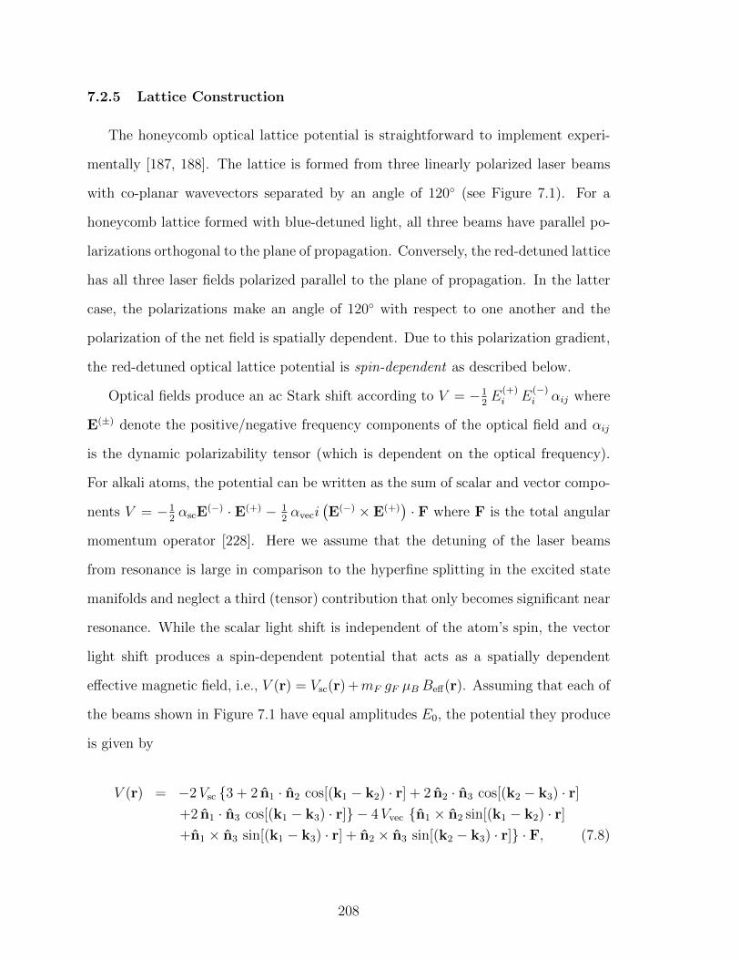
7.2.5 Lattice Construction

The honeycomb optical lattice potential is straightforward to implement experi-

mentally [187, 188]. The lattice is formed from three linearly polarized laser beams

with co-planar wavevectors separated by an angle of 120 (see Figure 7.1). For a

honeycomb lattice formed with blue-detuned light, all three beams have parallel po-

larizations orthogonal to the plane of propagation. Conversely, the red-detuned lattice

has all three laser fields polarized parallel to the plane of propagation. In the latter

case, the polarizations make an angle of 120 with respect to one another and the

polarization of the net field is spatially dependent. Due to this polarization gradient,

the red-detuned optical lattice potential is spin-dependent as described below.

Optical fields produce an ac Stark shift according to V = −12E

(+)i E

(−)i αij where

E(±) denote the positive/negative frequency components of the optical field and αij

is the dynamic polarizability tensor (which is dependent on the optical frequency).

For alkali atoms, the potential can be written as the sum of scalar and vector compo-

nents V = −12αscE

(−) · E(+) − 12αveci

(E(−) × E(+)

)· F where F is the total angular

momentum operator [228]. Here we assume that the detuning of the laser beams

from resonance is large in comparison to the hyperfine splitting in the excited state

manifolds and neglect a third (tensor) contribution that only becomes significant near

resonance. While the scalar light shift is independent of the atom’s spin, the vector

light shift produces a spin-dependent potential that acts as a spatially dependent

effective magnetic field, i.e., V (r) = Vsc(r) +mF gF µB Beff(r). Assuming that each of

the beams shown in Figure 7.1 have equal amplitudes E0, the potential they produce

is given by

V (r) = −2Vsc 3 + 2 n1 · n2 cos[(k1 − k2) · r] + 2 n2 · n3 cos[(k2 − k3) · r]

+2 n1 · n3 cos[(k1 − k3) · r] − 4Vvec n1 × n2 sin[(k1 − k2) · r]

+n1 × n3 sin[(k1 − k3) · r] + n2 × n3 sin[(k2 − k3) · r] · F, (7.8)

208

where ni are unit vectors denoting the polarization of each beam, Vsc = αscE20/8, and

Vvec = αvecE20/8. In Eq. 7.8 we have neglected to include relative phase differences

between the beams which only act to translate the lattice in two-dimensions without

changing its topology 7. The detuning from resonance controls the strength of the

vector light shift relative to that of the scalar light as described in Ref. [188]

The honeycomb lattice produced by the scalar light-shift is described by a hexago-

nal Bravais lattice with a two-point basis as shown in Figure 7.1(b). In a red-detuned

spin-dependent lattice, the depths of the A and B sublattices can be asymmetric,

e.g., |F,mF 〉 = |2, 1〉 or |1, 1〉, or symmetric, e.g., |F,mF 〉 = |1, 0〉, depending on the

internal state of the atom. An A/B sublattice asymmetry produces a mass gap at

the Dirac points.

7.2.6 Preparing a BEC at a Dirac Point

Study of the NLDE will require that the BEC be prepared at a Dirac point, i.e., K

or K′ in Figure 7.1(c). Several experimental methods can potentially accomplish this:

first, loading a BEC into the lowest-energy Bloch state and subsequently applying a

constant acceleration for a fixed duration; second, loading an initially stationary BEC

directly into a Bloch state at a Dirac point K by adiabatically applying a moving

lattice potential which maintains a constant velocity ~K/M ; and third, loading a

BEC into the lowest-energy Bloch state and subsequently populating a Dirac point

by Bragg scattering using auxiliary fields. The first two methods have potential

deficiencies. With regard to the first method, a dynamical instability may exist for

intermediate values of the crystal momenta as it linearly increases from 0 to K [229].

For the second method, the timescale required for adiabaticity is divergent since there

is no gap for crystal momenta along the Brillouin zone boundary in the absence of

a lattice potential. Hence, we consider here the method of populating a Dirac point

7If the relative phases between the beams vary slowly, the atoms will adiabatically follow theoptical lattice potential.

209

by inducing Bragg scattering between crystal momenta 0 and K using auxiliary laser

fields.

It is straightforward to populate the lowest-energy Bloch state of a honeycomb lat-

tice by adiabatically increasing the lattice depth as demonstrated in Ref. [188] where

both the BEC and the lattice are stationary in the lab frame. Here we will assume that

the BEC is in a hyperfine state with mF 6= 0 and a spin-dependent potential is used.

This is so that only the sublattice with the lowest energy, assumed here to be the A

sublattice, becomes occupied [188]. Starting from this initial condition, we can trans-

fer atoms to the Dirac point by Bragg scattering to thr associated Bloch state using

two laser fields with wavevectors kb1 and kb2. These obey the condition kb1−kb2 = K

such that ωb1 and ωb2. Also, we have that ωb1 − ωb2 = ∆ω = [EA(K) − EA(0)]/~.

Here, the function EA gives the dispersion relation for the lower (A) band of a hon-

eycomb lattice with A/B sublattice asymmetry. These fields produce a Stark shift

potential:

VBragg(r) =1

2VB [cos(K · r−∆ω t) + 1] , (7.9)

where VB sets the strength of the potential. This potential couples the Bloch wave-

functions ψA,K(r) = eiK·r uA,K(r) and ψA,0(r) = uA,0(r) where uA,K(r) and uA,0(r)

have the same periodicity as the lattice. Thus, both functions can be written in the

form

uA,K(r) =∑Q

CA,KQ eiQ·r, (7.10)

where the sum over Q includes all vectors in the reciprocal lattice space. The co-

efficients CA,KQ can be calculated for a honeycomb lattice of arbitrary scalar and

vector potential depths, Vsc and Vvec respectively, by numerically computing the band

structure for the potential given in Eq. 7.8 [77]. Application of the Bragg scattering

210

potential then results in Rabi oscillation between ψA,0 and ψA,K with a Rabi frequency

ΩB given by

ΩB =VB2 ~

∑Q

(CA,KQ )∗CA,0

Q . (7.11)

A particularly useful feature of using a honeycomb lattice potential with A/B

sublattice asymmetry for preparation is that both the initial and final Bloch states

(ψA,0 and ψA,K) have a group velocity relative to the lattice equal to zero. This is

because we are transferring atoms to a superposition of the two degenerate states at

the Dirac point: one with velocity cl and the other with velocity −cl. The former

state is continuously connected to “particle” excitations, when the crystal momentum

is increased, while the latter is continuously connected to “holes”. If the lattice is

stationary with respect to the lab frame, the condensate will then also be stationary

both before and after transfer to the Dirac point. This is experimentally convenient

since the condensate does not move out of the field of view and can remain confined

in an external trapping potential at all times. Note that the condensate would not

remain stationary if it were transferred to the Dirac point by Bragg scattering in

a lattice with A/B sublattice symmetry, i.e., no mass gap. In this case, the lower

and upper s-bands are degenerate at the Dirac point and the eigenstates can be

chosen from a two-dimensional subspace of degenerate states spanned by two Bloch

wavefunctions. Application of the VBragg potential breaks this degeneracy and excites

the eigenstate which moves in the same direction as that of the walking standing wave

potential VBragg with a group velocity having a magnitude of cl in the frame of the

lattice. The orthogonal eigenstate has a group velocity with the same magnitude but

in the opposite direction and is not coupled by VBragg to the Bloch state with zero

crystal momentum.

Once the condensate has been prepared at a Dirac point in a lattice with A/B

sublattice asymmetry by Bragg scattering, the atoms can be transferred to a hy-

211

perfine state that does not experience the vector light shift and therefore no mass

gap, e.g., |F,mF 〉 = |1, 1〉 → |1, 0〉, using a radio-frequency (rf) or microwave (mw)

field. For a spatially homogeneous rf/mw field, the transition matrix element is pro-

portional to the spatial overlap of the initial and final spatial wavefunctions which

are not orthogonal since they experience different lattice potentials. A spatially

homogeneous rf/mw field cannot change the crystal momentum which is therefore

conserved in the transition. In the absence of a vector light shift, the A and B

sublattices are symmetric and there is no mass gap, yielding two degenerate Bloch

states at the Dirac point K. Two orthogonal basis states that span the degenerate

subspace of eigenstates can be chosen to be states which have probability current

density j ≡ −i ~2M

(Ψ∗∇Ψ−Ψ∇Ψ∗) = 0 but are respectively localized on either

the A or B sublattice sites. A state prepared at the Dirac point of a lattice with

a mass gap will have significant spatial overlap with one of these basis states and

vanishing overlap with the orthogonal state. For example, for parameters identi-

cal to those realized in [188], i.e., Vsc = 4ER and Vvec/Vsc = 0.065. The mag-

nitude of the inner product between the initial and final states for wavefunctions

localized on the same sublattice is |〈A,K,mF = 1| A,K,mF = 0〉| = 0.995 whereas

|〈A,K,mF = 1| B,K,mF = 0〉| = 0. Thus, by driving a transition between internal

states with a rf/mw field, a condensate which remains stationary can be prepared

at the Dirac point of a honeycomb lattice with no mass gap. The state produced

will only have amplitude in sites of the A sublattice. In the next section we discuss

how the condensate can be coherently transferred between A and B sublattices by

modulating the lattice potential.

7.2.7 Coherent Transfer Between Sublattices

In relativistic quantum field theories, the vacuum state defines the lowest energy

configuration of the system. If massless particles appear in the spectrum, then excita-

tions of the vacuum may occur for arbitrarily small energetic disturbances. However,

212

for general interacting theories, particles may acquire a finite mass through radia-

tive corrections. In this case, we say that the interaction opens a mass gap in the

spectrum. The analogous concept for condensed matter systems is the presence of an

energy or band gap separating the highest filled single-particle states of the many-

body ground state from the lowest excitations of the system. In particular, for general

two-dimensional hexagonal lattices, a large number of possible gap-opening mecha-

nisms exist. For example, for electrons in graphene-like systems there are 36 possible

mass gaps which preserve particle-hole symmetry [155]. For bosons in a honeycomb

optical lattice, one way to open a mass gap is to introduce anisotropic tunneling be-

tween lattice sites. The ground state will then consist of alternating occupied and

unoccupied regions determined by the spatial modulation of the tunneling factors [16];

long-wavelength fluctuations will then be characterized by a finite excitation energy.

As previously discussed, we consider a system with A/B sublattice asymmetry

which has a mass gap 2 |ms| separating the s-bands of the A and B sublattices at

the Dirac point. Note that in the fully covariant NLDE, the mass gap will appear as

a factor of mcl multiplying the spinor wavefunction, where cl is the effective speed

of light. Transitions between Bloch states ψA,K and ψB,K can be driven by applying

a periodic perturbation Hm(r) cosωst where ~ωs = 2 |ms|, and Hm(r) is chosen to

exclusively couple pairs of Wannier states wA and wB localized on adjacent A and B

sites of a given unit cell, e.g., 〈wA(r− rA)|Hm |wB(r− r′A − δ1)〉 = ~Ωm δrA,r′A where

δ1 is the displacement between an A site and one of its three neighboring B sites.

A perturbation which only couples pairs of Wannier states separated by one of the

nearest neighbor displacement vectors, e.g., δ1, conserves the crystal momentum so

that 〈ψA,K+q|Hm |ψB,K+q′〉 = ei(K+q)·δ1 Ωm δq,q′ .

A suitable perturbation Hm can be experimentally realized by modulating the

amplitude of one of the lattice laser fields, which provides an anisotropic modulation

of the tunneling matrix elements that discriminates tunneling in one direction, while

213

simultaneously frequency modulating the other two fields, which periodically shakes

the lattice along the same direction. Amplitude modulation of the field E1 and

frequency modulation of E2 and E3 in Figure 7.1, for example, yields a periodic

perturbation with a spatial dependence given by

Hm(r) = Vm [cos(k1 − k2) · r + cos(k1 − k3) · r

+√

3Vvec

Vsc

mF sin(k1 − k2) · r + sin(k1 − k3) · r − κ δ1 · r], (7.12)

where κ depends on the relative amplitudes of the perturbations. The last term in

the square brackets describes shaking of the lattice along the δ1 direction while the

other terms act to anisotropically modulate the tunneling matrix elements between

nearest neighbors with tunneling in the δ1 direction distinguished from the other two.

The perturbations resulting from amplitude and frequency modulation both anisotrop-

ically couple a Wannier state wA to Wannier states wB localized on the three neigh-

boring sites, but discriminate tunneling in the δ1 direction with different relative

strengths. By adjusting the relative amplitude and phase of the two perturbations,

nearest neighbors in the δ1 direction can be strongly coupled with negligible coupling

to neighboring sites in the other two directions. For the experimental conditions re-

alized in Ref. [188], i.e., Vsc = 3.7ER and α = Vvec/Vsc = 0.065 for |mF | = 1 states of

87Rb atoms with λL = 830 nm, numerical solution [77] of Eq. (7.8) indicates that the

matrix elements 〈wA(r− rA)|Hm |wB(r− r′A − δ1)〉 ' 0.07Vm δrA,r′A are achieved for

κ ' 0.97 kL. The mass gap 2 |ms| = ~ (2π)×9.4 kHz in this case. For Vm = 0.325ER,

the Rabi frequency Ωm = (2π) × 75 Hz and complete sublattice transfer is attained

by applying the perturbation for a time Ωm/π = 7 ms which has sufficient spectral

resolution to resolve transitions to other bands.

To coherently transfer a condensate between sublattices when the condensate is

initially in an internal state withmF = 0, which does not experience an A/B sublattice

asymmetry, an rf/mw transition can be applied to couple to an intermediate internal

214

state with mF 6= 0 that does experience an A/B sublattice asymmetry. Modulation of

the lattice potential with the perturbation Hm(r) cosωmt can then be applied to drive

transitions between the A and B sublattices as described above provided that ~ωm

equals the mass gap for the condensate with mF 6= 0. The atoms can be subsequently

transferred back to the original internal state via an ensuing rf/mw transition.

If the rf/mw and lattice modulation frequencies are detuned from resonance with

the intermediate states, this sequence of transitions behaves as a direct transition

between Bloch states |i〉 = |ψA,K〉 and |f〉 = |ψB,K〉 with an effective Rabi frequency

ΩAB given by

ΩAB =Ωmw1 Ωm Ωmw2

∆mw1 ∆mw2

. (7.13)

The parameters ∆mw1 and ∆mw2 control the detunings from the intermediate states.

The parameters Ωmw1, Ωm, and Ωmw2 are the Rabi frequencies associated with the

transitions out of the initial mF = 0 state, from the A sublattice to the B sublattice,

and finally back to the initial mF = 0 state, respectively.

7.2.8 Creation of Vortices

In this section, we discuss how relativistic vortex solutions of the NLDE can be

excited by modifying the technique for coherent sublattice transfer described in the

previous section. The two-photon Raman transition drives Rabi oscillations between

two hyperfine states in the electronic ground state of an atom by coupling through

intermediate states which are optically excited electronic states. The transition ma-

trix element between hyperfine states is proportional to the product of the two field

amplitudes which drive the two-photon transition. To excite a vortex, the two optical

fields are provided by co-propagating Gaussian and Laguerre-Gaussian laser beams

which have a frequency difference corresponding to the energy splitting between the

initial and final states but are both far-detuned from the intermediate states to reduce

215

spontaneous emission. The Laguerre-Gaussian beam carries a single unit of orbital

angular momentum which is transferred to the atoms in the stimulated Raman transi-

tion [191]. The electric field amplitude of a Laguerre-Gaussian laser beam with radial

mode index p = 0 and charge index ` = 1 is proportional to

Ep=0,`=1LG (r, θ) ∝ r exp

(− r

2

w20

)exp(iθ), (7.14)

where r and θ are respectively the radial and azimuthal coordinates relative to the

optical axis and w0 is the beam waist. The field of the Gaussian laser beam EG(r, θ) ∝

exp(− r2

w20

). Thus, the effective Rabi frequency for the two photon transition Ω2γ ∝

〈f |EG(r)Ep=0,`=1LG (r) |I2〉 where |I2〉 and |f〉 are respectively the intermediate and

final state spatial wavefunctions of the condensate. Due to the azimuthal phase

winding exp(iθ) of the LG field Ep=0,`=1LG , the Raman fields provide the appropriate

spatial dependence to drive a transition to a final state |f〉 which has a single unit of

angular momentum starting from the intermediate state |I2〉 with no orbital angular

momentum.

Starting from a condensate at the Dirac point K with amplitude only in the A

sublattice sites, i.e., the Bloch state ψA,K, the procedure described above would couple

to a vortex/soliton solution of the NLDE which has a vortex in the B sublattice and a

soliton, with no angular momentum, in the A sublattice. This solution of the NLDE

in the continuum limit can be written as a Weyl spinor of the form Ψf = (ψA, ψB) =

(ifA(r), fB(r)eiθ) (see Sect. 7.3 below and Ref. [184]). The initial wavefunction of the

condensate at the Dirac point ψA,K is described by the Weyl spinor Ψi = (ψA, ψB) =

(1, 0). Starting from the state |i〉 = ψmF =0A,K , the transition proceeds to an intermediate

state with mF = 1 at the Dirac point of the A sublattice (i.e. |I1〉 = ψmF =1A,K ), then to

the B sublattice (i.e. |I2〉 = ψmF =1B,K ) by modulation of the lattice potential through

application of Hm cosωmt. Finally, by the two-photon Raman transition, we obtain

the final state |f〉. This is the vortex/soliton state in the internal state with mF = 0.

216

If we assume that w0, ξ a and take the tight binding and continuum limits, the

effective Rabi Raman frequency

Ω2γ ∝ 〈I2|EG(r)Ep=0,`=1LG (r) |f〉 (7.15)

∝ EG,0ELG,0

∫dr fB(r) r2 e−2r2/w2

0 .

The radial dependence of the vortex in the B sublattice fB(r) is calculated below (see

Sect. 7.3). The radial integral is positive definite and for w0 ∼ ξ will give a non-zero

Rabi frequency with an absolute value determined by the amplitudes of the fields

driving the two-photon Raman transition and the dipole transition matrix elements

for the 5S-5P electronic transitions in 87Rb.

7.2.9 Coherent Transfer Between Dirac Points by Bragg Scattering

Once a BEC has been prepared at a Dirac point K, coherent transfer to the non-

equivalent Dirac point K′ can be accomplished by Bragg scattering from a lattice

formed using auxiliary laser fields [189]. In this case, the two additional laser fields

have wavevectors kb1 and kb2 where kb1 − kb2 = K′ − K = −kL y in the frame of

the lattice. The lattice produced by these fields couples a BEC at crystal momentum

K = kL

(√3

2x + 1

2y)

to a BEC with crystal momentum K′ = kL

(√3

2x− 1

2y)

by

Bragg scattering. Since the energies of the two coupled Dirac points are identical,

resonance occurs when the optical frequencies of the auxiliary fields are equal and the

standing wave they form is stationary in the frame of the honeycomb lattice.

In the frame of the lattice, the applied potential is

VBragg(r) =1

2VB [cos(K−K′) · r + 1] . (7.16)

This potential couples the degenerate Bloch wavefunctions ψK(r) and ψK′(r). The

matrix element coupling ψK and ψK′ is then given by

217

Ωα,βB =

VB2 ~

∑Q

(Cα,K′

Q

)∗Cβ,K

Q , (7.17)

where the coefficients Cα,KQ are identical to those defined in Sect. 7.2.6 where the index

α designates the sublattice on which the condensate is localized. These coefficients

can be found by numerically computing the band structure for the potential given in

Eq. (7.8) [77]. Note that there are four degenerate Bloch wavefunctions correspond-

ing to the two possible inequivalent Dirac points (K and K′) and the two possible

sublattices (A and B). In the tight-binding limit, i.e., Vsc ER, the Bragg scattering

lattice only couples Bloch states at the non-equivalent Dirac points that are localized

on the same sublattice. In this limit, application of the Bragg scattering lattice will

induce Rabi oscillations with frequency Ωα,αB between condensates localized on the

same sublattice but at the non-equivalent Dirac points. For shallower depths of the

honeycomb lattice, all four degenerate Bloch states will be coupled and the dynamics

will be more complicated. However, even for a moderate lattice depth Vsc = 4ER, the

coupling between different sublattices is small enough that the dynamics are nearly

identical to those of two coupled Bloch states.

Starting from a BEC initially prepared at a single Dirac point K, application of the

Bragg scattering potential will cause the amplitude to Rabi oscillate between ψK and

ψK′ with a Rabi oscillation frequency ΩBragg = 2 |〈K′ |VBragg|K〉|. The pulse duration

of the auxiliary fields can be controlled to produce an arbitrary superposition of BECs

at K and K′ – with a π2-pulse τπ/2 = π

21

ΩBraggproducing an equal superposition.

7.3 Vortex Solutions of the NLDE

The NLDE describes the dynamics of a four-spinor, Ψ ≡ (Ψ+, Ψ−)T , with the

upper (+) and lower (−) two-spinors relating to opposite K and K′ points of the

honeycomb lattice:

218

iγµ∂µΨ− U4∑i=1

(MiΨ)(Ψ†Mi) Ψ = 0 . (7.18)

The matrices γµ are the usual Dirac matrices and the interaction terms are encapsu-

lated in the summation with the matrices Mi constructed to give the correct cubic

nonlinearites, local to each spinor component [52]. This describes a gapless theory

which corresponds to massless interacting Dirac spinors. Since the interactions do not

couple different spinor components, Eq. (8.3) can be split into two sets of equations

(one for each of the K and K′ points) of the form

i~ ∂tψA = −i~cl (∂x − i∂y)ψB + U |ψA|2 ψA (7.19)

i~ ∂tψB = −i~cl (∂x + i∂y)ψA + U |ψB|2 ψB , (7.20)

with the full solution expressed as a linear combination of solutions from each Dirac

point. Note the presence of the effective speed of light, cl, and interaction strength,

U . We first look for solutions with cylindrical symmetry, i.e., vortex solutions with

arbitrary integer phase winding in addition to bright soliton solutions. We can ob-

tain a dimensionless form of the NLDE by expressing the spinor wavefunctions as:

ψA(r, θ, t) = ±i fA(r)ei(`−1)θ e−iµt/~, ψB(r, θ, t) = fB(r)ei`θ e−iµt/~, where ` is the in-

teger vortex winding and µ is the chemical potential. In plane-polar coordinates,

Eqs. (8.4)-(8.5) become

−~cl(∂r +

`

r

)fB(r) + U |fA(r)|2fA(r) = µfA(r) (7.21)

~cl(∂r +

1−`r

)fA(r) + U |fB(r)|2fB(r) = µfB(r). (7.22)

Localized solutions of the NLDE may be categorized by their asymptotic forms, i.e.,

whether the amplitude has a zero or non-zero limit far from the core. This differ-

ence is significant since it is fundamentally related to the presence (or absence) of

219

an underlying topological structure. Solutions for which one or both spinor compo-

nents are finite far from the core are topological : they may be derived as extrema for

Lagrangians having effective potentials which exhibit at least one (or several) local

minimum (minima) separated from the ground state (or saddle point solution) energy

by a finite barrier in solution space. All other solutions, for which both spinor com-

ponents fall to zero far from the core, do not have an underlying topological structure

and are referred to as non-topological.

7.3.1 Asymptotic Bessel Solutions for Large Phase Winding

For integer winding ` ≥ 2, both fA and fB must vanish at r = 0 due to the

presence of the centrifugal terms, so we will treat the special cases ` = 0, 1 in a

separate section. To obtain vortex solutions, we require spatial derivatives to vanish

at infinity, so that for r → ∞, Eqs. (8.6)-(8.7) yield the possible asymptotic forms:

fA(B)(∞)[|fA(B)(∞)|2 − µ/U

]= 0 or fA(B)(∞) ∼ rα, for 0 < α < 1. The first case

implies∣∣fA(B)(∞)

∣∣ = 0, ±√µ/U . For the case of non-vanishing boundary conditions

and ` ≥ 2, the asymmetry in the angular momentum terms of the NLDE seems

problematic. We recall that the factors ∂r+`/r and ∂r+(1−`)/r act as index raising

and lowering operators for the Bessel functions Jn. This becomes clear when we check

that Bessel functions are exact solutions in the zero interaction or low density limit

given by ~cl/U |Ψ|2 1. In this limit, solutions of Eqs. (8.6)-(8.7) are Bessel functions

of the first kind, Jl and Jl−1, only slightly modified by the weak interaction terms

which describe scattering into other Bessel functions. We then choose the modified

Bessel-Fourier expansion as our ansatz

fA(r) = AF (r) eiQ(r)

[a0 +

∞∑n=1

anJn(r)

](7.23)

fB(r) = (B/A) fA(r) , (7.24)

220

where A and B are normalization constants, Jn(r) is the Bessel function of the first

kind of order n, a0 and an are the expansion coefficients, and Q(r) is the argument of

the integrating factor, which we include to enlarge the parameter space. The series

that we have chosen to use runs over the Bessel index rather than the usual form

where the summation runs over the zeros of one Bessel function with fixed index. Our

choice of expansion is certainly valid but does not offer the convenience of using the

standard orthonormal relations for Bessel functions when computing the coefficients.

Once the ansatz is substituted into the NLDE, we combine the angular momentum

and derivative terms in the series by using the recurrence relations for Bessel functions:

Jn/x=(Jn−1+Jn+1)/2n and J ′n=(Jn−1−Jn+1)/2. Substituting Eqs. (7.23)-(7.24) into

Eqs. (8.6)-(8.7) gives two first-order differential equations for the integrating factor

Q in addition to the recursion relations for the coefficients an. We find that Q must

solve the first order equation

iQ′ = −F′

F− a0`

r± U

~cli|AF |2

∣∣∣∣∣a0+∑n

anJn

∣∣∣∣∣2

∓ i µ~cl

a0 +∑

nC′nanJn

a0 +∑

nanJn, (7.25)

in addition to a similar equation but where ` is replaced by 1 − `. The recursion

relations for the an are

an+1

2

(`+ n+ 1

n+ 1

)+an−1

2

(`− n+ 1

n− 1

)= − µA

~clBCnan

an+1

2

(2− `+ n

n+ 1

)+an−1

2

(2− `− nn− 1

)=

µB

~clACnan.

(7.26)

In Eq. (7.25) we have absorbed a term-dependent fraction Cn ≡ 1 − C ′n, from the

chemical potential terms, into the recursion relations. We can solve the recursion

relations to get

A = ±iB , an =

(± i C µ

U(2`− 1)

)n−1n !

nn−1. (7.27)

221

To obtain a vortex solution, we set a0 = −1/2` which cancels the factor of F (r) in

Eq. (7.25), provided F = r1/2. This effectively allows the solution to vanish at the

origin and also balances the behavior of the Bessel functions at long distances. The

vortex solution is obtained by tuning the parameter C in Eq. (7.27) to some critical

value Cvortex. If we examine the asymptotic region r ξDirac, far from the vortex

core, the Bessel functions decrease at a rate proportional to r−1/2. On the other hand,

near the vortex core where r ξDirac, the Bessel functions have the form Jn ∼ rn,

for n ≥ 1. Using this information, in the regions r ξDirac and r ξDirac, and for

weak interaction U , we obtain the asymptotic integral solution of Eq. (7.25)

iQ ≈ ± i µ~cl

r . (7.28)

The vortex profile is obtained for `2 1 and for the values Cvortex = 2.5 × (2` − 1)

and µ/U = 1. We have plotted this solution in Figure 7.6(a) which has a closed form

given by

fA(r) = A(Ur/~cl)1/2 e±i(Ur/~cl)∞∑n=1

(2.5 i)n−1 n !

nn−1Jn(Ur/~cl) , (7.29)

where the overall constant A is determined by normalizing the wavefunction. Density

and phase plots for the complex Bessel solution are shown in Figure 7.4.

7.3.2 Numerical Shooting Method for Vortices with Arbitrary PhaseWinding and Chemical Potential

The radial profile for a topological vortex with arbitrary winding number ` can

be obtained using a numerical shooting method [230]. The most direct approach is

to express Eqs. (8.6)-(8.7) in terms of the dimensionless radial variable χ ≡ (U/~cl)r.

The functions fA(χ) and fB(χ) are then expanded in power series around χ = 0:

fA(χ) =∞∑j=0

ajχj , fB(χ) =

∞∑j=0

bjχj , (7.30)

222

where the aj and bj are the expansion coefficients. Since we are solving two coupled

first order equations, we require the initial conditions fA(0) and fB(0). Substituting

into Eqs. (8.6)-(8.7) gives us the core behavior

fA(0) ∼ χ`−1 , fB(0) ∼ χ` . (7.31)

These core values indicate that the first nonzero coefficients for a given choice of `

are a`−1 and b`, where a`−1 is sufficient to determine all other coefficients for both

expansions in Eq. (8.41). For a given ` value, a vortex is found by tuning a`−1 towards

a critical value avortex`−1 . As examples, we have found vortices for the three lowest `

values for which both spinor components have nonzero rotation:

avortex1 = 0.571718... , ` = 2 , (7.32)

avortex2 = 0.145291... , ` = 3 , (7.33)

avortex3 = 0.0240267... , ` = 4 . (7.34)

In Figure 7.2 we have plotted both components for the case ` = 2 and illustrated

the convergence to the vortex solution by overlaying an excitation of the vortex (a)

and the free particle Bessel solution (b). The ` = 4 numerical topological vortex

solution density and phase are shown in Figure 7.5 and the radial solution plotted

in Figure 7.6(b).

The same shooting method can be used to obtain the ring-vortex solutions for

the special case of the chemical potential µ = 0. These types of solutions are non-

topological vortices whose tails decay to zero far from core. Although we demonstrate

such solutions by analytical methods in the next section, the numerical approach

allows us to illustrate the transition from the vortex limit (µ U) to Bessel solutions

in the free particle limit (µ U). This transition is illustrated in Figure 7.3 for the

strength of the nonlinearity U fixed to unity and the chemical potential running from

0.001 to 2. In Sec. 7.4, we provide a more thorough discussion of our numerical

223

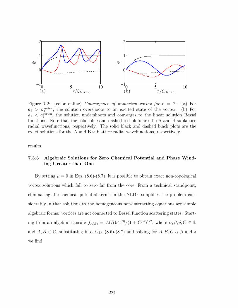
0 5 10−1

0

1

2

(a) r/ξDirac

Ψ

0 5 10−1

0

1

2

(b) r/ξDirac

Ψ

Figure 7.2: (color online) Convergence of numerical vortex for ` = 2. (a) Fora1 > avortex

1 , the solution overshoots to an excited state of the vortex. (b) Fora1 < avortex

1 , the solution undershoots and converges to the linear solution Besselfunctions. Note that the solid blue and dashed red plots are the A and B sublatticeradial wavefunctions, respectively. The solid black and dashed black plots are theexact solutions for the A and B sublattice radial wavefunctions, respectively.

results.

7.3.3 Algebraic Solutions for Zero Chemical Potential and Phase Wind-ing Greater than One

By setting µ = 0 in Eqs. (8.6)-(8.7), it is possible to obtain exact non-topological

vortex solutions which fall to zero far from the core. From a technical standpoint,

eliminating the chemical potential terms in the NLDE simplifies the problem con-

siderably in that solutions to the homogeneous non-interacting equations are simple

algebraic forms: vortices are not connected to Bessel function scattering states. Start-

ing from an algebraic ansatz fA(B) = A(B)rα(β)/(1 + Crδ)1/2, where α, β, δ, C ∈ R

and A,B ∈ C, substituting into Eqs. (8.6)-(8.7) and solving for A,B,C, α, β and δ

we find

224

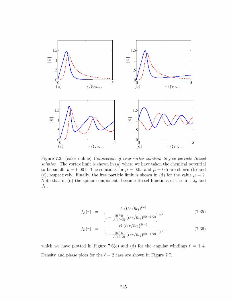
0 50

.5

1

1.5

(a) r/ξDirac

|Ψ|

0 50

.5

1

1.5

(b) r/ξDirac

|Ψ|

0 50

.5

1

1.5

(c) r/ξDirac

|Ψ|

0 50

.5

1

1.5

(d) r/ξDirac

|Ψ|

Figure 7.3: (color online) Connection of ring-vortex solution to free particle Besselsolution. The vortex limit is shown in (a) where we have taken the chemical potentialto be small: µ = 0.001. The solutions for µ = 0.05 and µ = 0.5 are shown (b) and(c), respectively. Finally, the free particle limit is shown in (d) for the value µ = 2.Note that in (d) the spinor components become Bessel functions of the first J0 andJ1 .

fA(r) =A (Ur/~cl)`−1[

1 + |B|2BA(4`−2)

(Ur/~cl)8(`−1/2)]1/2

(7.35)

fB(r) =B (Ur/~cl)3`−2[

1 + |B|2BA(4`−2)

(Ur/~cl)8(`−1/2)]1/2

, (7.36)

which we have plotted in Figure 7.6(c) and (d) for the angular windings ` = 1, 4.

Density and phase plots for the ` = 2 case are shown in Figure 7.7.

225

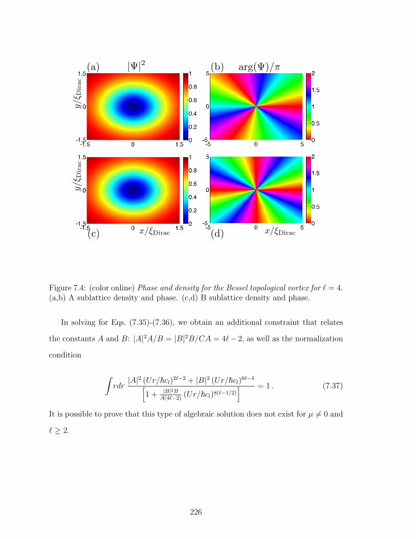
x/ξDiracx/ξDirac

y/ξ D

irac

y/ξ

Dirac

|Ψ|2 arg(Ψ)/π(a) (b)

(c) (d)

Figure 7.4: (color online) Phase and density for the Bessel topological vortex for ` = 4.(a,b) A sublattice density and phase. (c,d) B sublattice density and phase.

In solving for Eqs. (7.35)-(7.36), we obtain an additional constraint that relates

the constants A and B: |A|2A/B = |B|2B/CA = 4`− 2, as well as the normalization

condition

∫rdr|A|2 (Ur/~cl)2`−2 + |B|2 (Ur/~cl)6`−4[

1 + |B|2BA(4`−2)

(Ur/~cl)8(`−1/2)] = 1 . (7.37)

It is possible to prove that this type of algebraic solution does not exist for µ 6= 0 and

` ≥ 2.

226

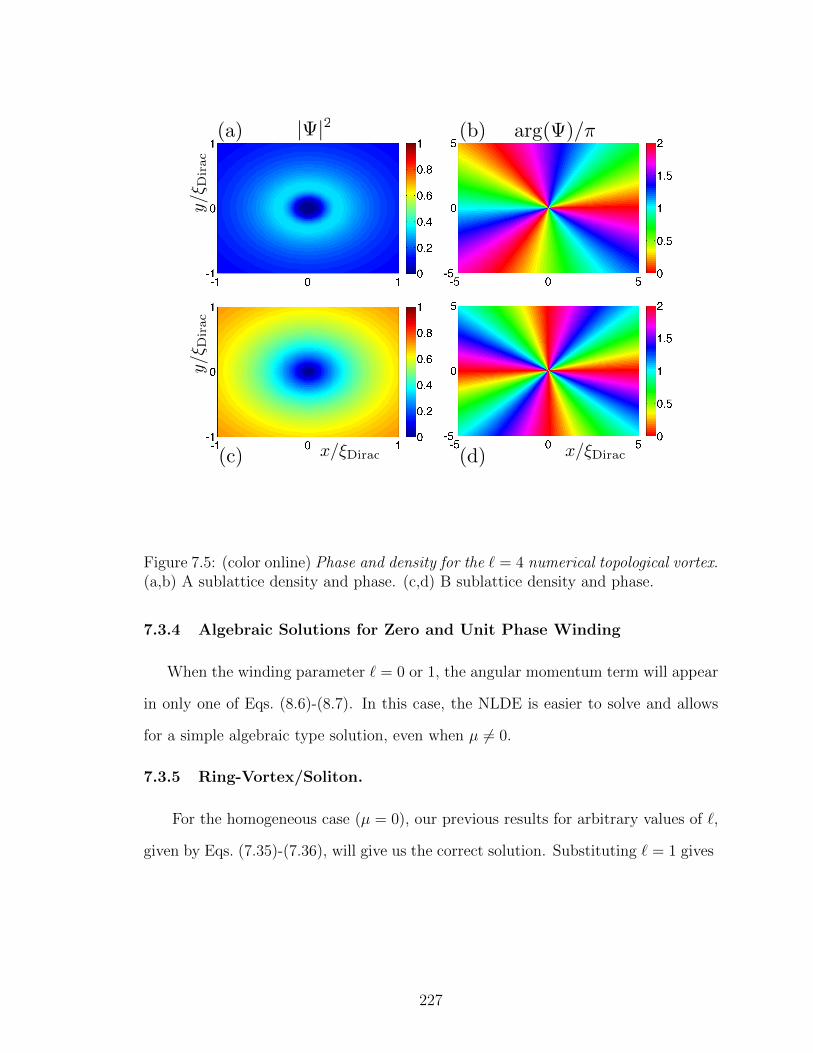
x/ξDiracx/ξDirac

y/ξ D

irac

y/ξ

Dirac

|Ψ|2 arg(Ψ)/π(a) (b)

(c) (d)

Figure 7.5: (color online) Phase and density for the ` = 4 numerical topological vortex.(a,b) A sublattice density and phase. (c,d) B sublattice density and phase.

7.3.4 Algebraic Solutions for Zero and Unit Phase Winding

When the winding parameter ` = 0 or 1, the angular momentum term will appear

in only one of Eqs. (8.6)-(8.7). In this case, the NLDE is easier to solve and allows

for a simple algebraic type solution, even when µ 6= 0.

7.3.5 Ring-Vortex/Soliton.

For the homogeneous case (µ = 0), our previous results for arbitrary values of `,

given by Eqs. (7.35)-(7.36), will give us the correct solution. Substituting ` = 1 gives

227

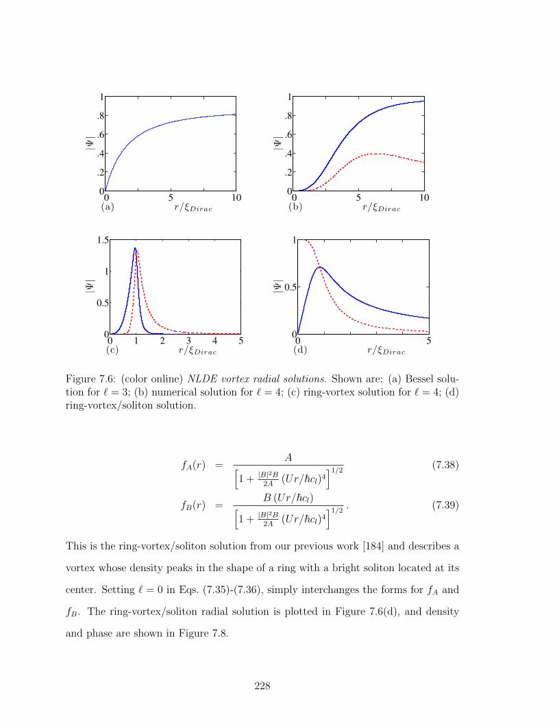
0 5 100

.2

.4

.6

.8

1

(a) r/ξDirac

|Ψ|

0 5 100

.2

.4

.6

.8

1

(b) r/ξDirac

|Ψ|

0 1 2 3 4 50

0.5

1

1.5

(c) r/ξDirac

|Ψ|

0 50

0.5

1

(d) r/ξDirac

|Ψ|

Figure 7.6: (color online) NLDE vortex radial solutions. Shown are: (a) Bessel solu-tion for ` = 3; (b) numerical solution for ` = 4; (c) ring-vortex solution for ` = 4; (d)ring-vortex/soliton solution.

fA(r) =A[

1 + |B|2B2A

(Ur/~cl)4]1/2

(7.38)

fB(r) =B (Ur/~cl)[

1 + |B|2B2A

(Ur/~cl)4]1/2

. (7.39)

This is the ring-vortex/soliton solution from our previous work [184] and describes a

vortex whose density peaks in the shape of a ring with a bright soliton located at its

center. Setting ` = 0 in Eqs. (7.35)-(7.36), simply interchanges the forms for fA and

fB. The ring-vortex/soliton radial solution is plotted in Figure 7.6(d), and density

and phase are shown in Figure 7.8.

228

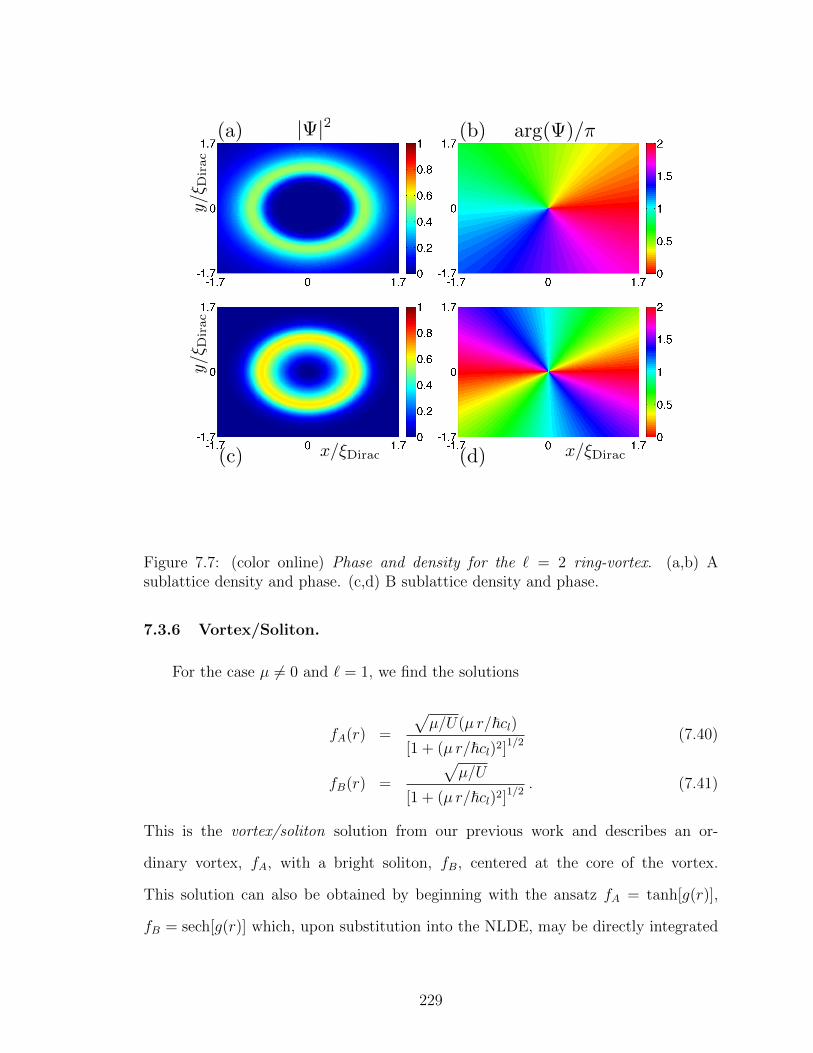
x/ξDiracx/ξDirac

y/ξ D

irac

y/ξ

Dirac

|Ψ|2 arg(Ψ)/π(a) (b)

(c) (d)

Figure 7.7: (color online) Phase and density for the ` = 2 ring-vortex. (a,b) Asublattice density and phase. (c,d) B sublattice density and phase.

7.3.6 Vortex/Soliton.

For the case µ 6= 0 and ` = 1, we find the solutions

fA(r) =

√µ/U(µ r/~cl)

[1 + (µ r/~cl)2]1/2(7.40)

fB(r) =

õ/U

[1 + (µ r/~cl)2]1/2. (7.41)

This is the vortex/soliton solution from our previous work and describes an or-

dinary vortex, fA, with a bright soliton, fB, centered at the core of the vortex.

This solution can also be obtained by beginning with the ansatz fA = tanh[g(r)],

fB = sech[g(r)] which, upon substitution into the NLDE, may be directly integrated

229

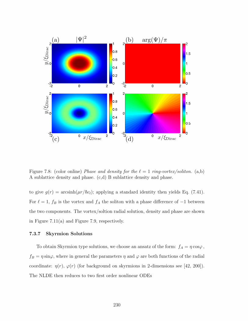
x/ξDiracx/ξDirac

y/ξ D

irac

y/ξ

Dirac

|Ψ|2 arg(Ψ)/π(a) (b)

(c) (d)

Figure 7.8: (color online) Phase and density for the ` = 1 ring-vortex/soliton. (a,b)A sublattice density and phase. (c,d) B sublattice density and phase.

to give g(r) = arcsinh(µr/~cl); applying a standard identity then yields Eq. (7.41).

For ` = 1, fB is the vortex and fA the soliton with a phase difference of −1 between

the two components. The vortex/soltion radial solution, density and phase are shown

in Figure 7.11(a) and Figure 7.9, respectively.

7.3.7 Skyrmion Solutions

To obtain Skyrmion type solutions, we choose an ansatz of the form: fA = η cosϕ ,

fB = η sinϕ, where in general the parameters η and ϕ are both functions of the radial

coordinate: η(r), ϕ(r) (for background on skyrmions in 2-dimensions see [42, 200]).

The NLDE then reduces to two first order nonlinear ODEs

230

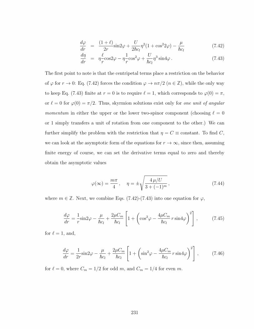
dϕ

dr=

(1 + `)

2rsin2ϕ+

U

2~clη2(1 + cos22ϕ)− µ

~cl(7.42)

dη

dr= η

`

rcos2ϕ− η1

rcos2ϕ+

U

~clη3 sin4ϕ . (7.43)

The first point to note is that the centripetal terms place a restriction on the behavior

of ϕ for r → 0: Eq. (7.42) forces the condition ϕ→ nπ/2 (n ∈ Z), while the only way

to keep Eq. (7.43) finite at r = 0 is to require ` = 1, which corresponds to ϕ(0) = π,

or ` = 0 for ϕ(0) = π/2. Thus, skyrmion solutions exist only for one unit of angular

momentum in either the upper or the lower two-spinor component (choosing ` = 0

or 1 simply transfers a unit of rotation from one component to the other.) We can

further simplify the problem with the restriction that η = C ≡ constant. To find C,

we can look at the asymptotic form of the equations for r →∞, since then, assuming

finite energy of course, we can set the derivative terms equal to zero and thereby

obtain the asymptotic values

ϕ(∞) =mπ

4, η = ±

√4µ/U

3 + (−1)m, (7.44)

where m ∈ Z. Next, we combine Eqs. (7.42)-(7.43) into one equation for ϕ,

dϕ

dr=

1

rsin2ϕ− µ

~cl+

2µCm~cl

[1 +

(cos2ϕ− 4µCm

~clr sin4ϕ

)2], (7.45)

for ` = 1, and,

dϕ

dr=

1

2rsin2ϕ− µ

~cl+

2µCm~cl

[1 +

(sin2ϕ− 4µCm

~clr sin4ϕ

)2], (7.46)

for ` = 0, where Cm = 1/2 for odd m, and Cm = 1/4 for even m.

231

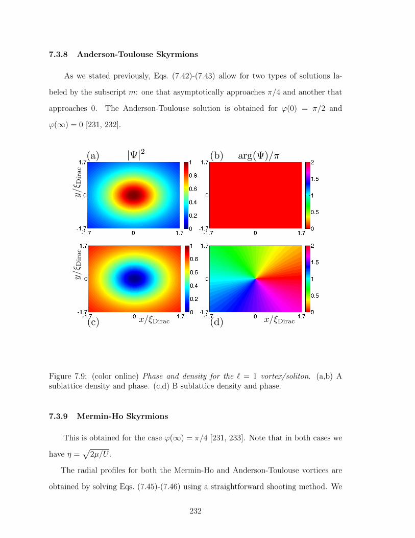
7.3.8 Anderson-Toulouse Skyrmions

As we stated previously, Eqs. (7.42)-(7.43) allow for two types of solutions la-

beled by the subscript m: one that asymptotically approaches π/4 and another that

approaches 0. The Anderson-Toulouse solution is obtained for ϕ(0) = π/2 and

ϕ(∞) = 0 [231, 232].

x/ξDiracx/ξDirac

y/ξ D

irac

y/ξ

Dirac

|Ψ|2 arg(Ψ)/π(a) (b)

(c) (d)

Figure 7.9: (color online) Phase and density for the ` = 1 vortex/soliton. (a,b) Asublattice density and phase. (c,d) B sublattice density and phase.

7.3.9 Mermin-Ho Skyrmions

This is obtained for the case ϕ(∞) = π/4 [231, 233]. Note that in both cases we

have η =√

2µ/U .

The radial profiles for both the Mermin-Ho and Anderson-Toulouse vortices are

obtained by solving Eqs. (7.45)-(7.46) using a straightforward shooting method. We

232

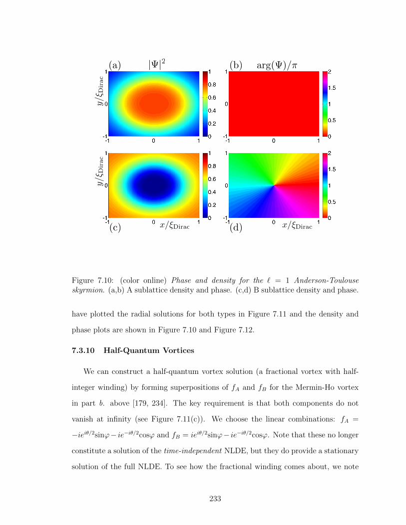
x/ξDiracx/ξDirac

y/ξ D

irac

y/ξ

Dirac

|Ψ|2 arg(Ψ)/π(a) (b)

(c) (d)

Figure 7.10: (color online) Phase and density for the ` = 1 Anderson-Toulouseskyrmion. (a,b) A sublattice density and phase. (c,d) B sublattice density and phase.

have plotted the radial solutions for both types in Figure 7.11 and the density and

phase plots are shown in Figure 7.10 and Figure 7.12.

7.3.10 Half-Quantum Vortices

We can construct a half-quantum vortex solution (a fractional vortex with half-

integer winding) by forming superpositions of fA and fB for the Mermin-Ho vortex

in part b. above [179, 234]. The key requirement is that both components do not

vanish at infinity (see Figure 7.11(c)). We choose the linear combinations: fA =

−ieiθ/2sinϕ− ie−iθ/2cosϕ and fB = ieiθ/2sinϕ− ie−iθ/2cosϕ. Note that these no longer

constitute a solution of the time-independent NLDE, but they do provide a stationary

solution of the full NLDE. To see how the fractional winding comes about, we note

233

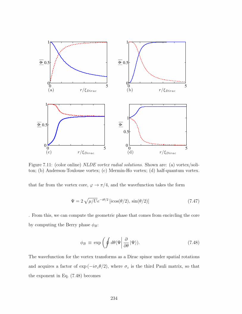
0 50

0.5

1

(a) r/ξDirac

|Ψ|

0 50

0.5

1

(b) r/ξDirac

|Ψ|

0 50

0.5

1

(c) r/ξDirac

|Ψ|

0 50

0.5

1

(d) r/ξDirac

|Ψ|

Figure 7.11: (color online) NLDE vortex radial solutions. Shown are: (a) vortex/soli-ton; (b) Anderson-Toulouse vortex; (c) Mermin-Ho vortex; (d) half-quantum vortex.

that far from the vortex core, ϕ→ π/4, and the wavefunction takes the form

Ψ = 2√µ/Ue−iθ/2 [icos(θ/2), sin(θ/2)] (7.47)

. From this, we can compute the geometric phase that comes from encircling the core

by computing the Berry phase φB:

φB ≡ exp

(∮dθ〈Ψ

∣∣∣∣ ∂∂θ |Ψ〉). (7.48)

The wavefunction for the vortex transforms as a Dirac spinor under spatial rotations

and acquires a factor of exp (−iσzθ/2), where σz is the third Pauli matrix, so that

the exponent in Eq. (7.48) becomes

234

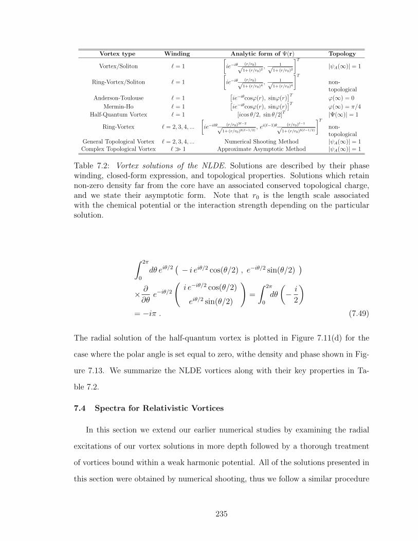
Vortex type Winding Analytic form of Ψ(r) Topology

Vortex/Soliton ` = 1

[ie−iθ (r/r0)√

1+ (r/r0)2, 1√

1+ (r/r0)2

]T|ψA(∞)| = 1

Ring-Vortex/Soliton ` = 1

[ie−iθ (r/r0)√

1+ (r/r0)4, 1√

1+ (r/r0)4

]Tnon-topological

Anderson-Toulouse ` = 1[ie−iθcosϕ(r), sinϕ(r)

]Tϕ(∞) = 0

Mermin-Ho ` = 1[ie−iθcosϕ(r), sinϕ(r)

]Tϕ(∞) = π/4

Half-Quantum Vortex ` = 1 [icos θ/2, sin θ/2]T |Ψ(∞)| = 1

Ring-Vortex ` = 2, 3, 4, ...

[ie−i`θ (r/r0)3`−2√

1+ (r/r0)8(`−1/2), ei(`−1)θ (r/r0)`−1√

1+ (r/r0)8(`−1/2)

]Tnon-topological

General Topological Vortex ` = 2, 3, 4, ... Numerical Shooting Method |ψA(∞)| = 1Complex Topological Vortex ` 1 Approximate Asymptotic Method |ψA(∞)| = 1

Table 7.2: Vortex solutions of the NLDE. Solutions are described by their phasewinding, closed-form expression, and topological properties. Solutions which retainnon-zero density far from the core have an associated conserved topological charge,and we state their asymptotic form. Note that r0 is the length scale associatedwith the chemical potential or the interaction strength depending on the particularsolution.

∫ 2π

0

dθ eiθ/2(− i eiθ/2 cos(θ/2) , e−iθ/2 sin(θ/2)

)× ∂

∂θe−iθ/2

(i e−iθ/2 cos(θ/2)

eiθ/2 sin(θ/2)

)=

∫ 2π

0

dθ

(− i

2

)= −iπ . (7.49)

The radial solution of the half-quantum vortex is plotted in Figure 7.11(d) for the

case where the polar angle is set equal to zero, withe density and phase shown in Fig-

ure 7.13. We summarize the NLDE vortices along with their key properties in Ta-

ble 7.2.

7.4 Spectra for Relativistic Vortices

In this section we extend our earlier numerical studies by examining the radial

excitations of our vortex solutions in more depth followed by a thorough treatment

of vortices bound within a weak harmonic potential. All of the solutions presented in

this section were obtained by numerical shooting, thus we follow a similar procedure

235

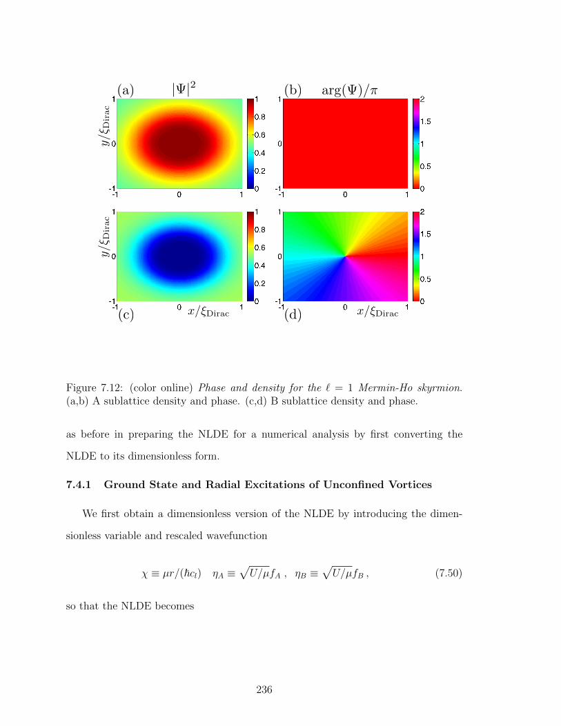
x/ξDiracx/ξDirac

y/ξ D

irac

y/ξ

Dirac

|Ψ|2 arg(Ψ)/π(a) (b)

(c) (d)

Figure 7.12: (color online) Phase and density for the ` = 1 Mermin-Ho skyrmion.(a,b) A sublattice density and phase. (c,d) B sublattice density and phase.

as before in preparing the NLDE for a numerical analysis by first converting the

NLDE to its dimensionless form.

7.4.1 Ground State and Radial Excitations of Unconfined Vortices

We first obtain a dimensionless version of the NLDE by introducing the dimen-

sionless variable and rescaled wavefunction

χ ≡ µr/(~cl) ηA ≡√U/µfA , ηB ≡

√U/µfB , (7.50)

so that the NLDE becomes

236

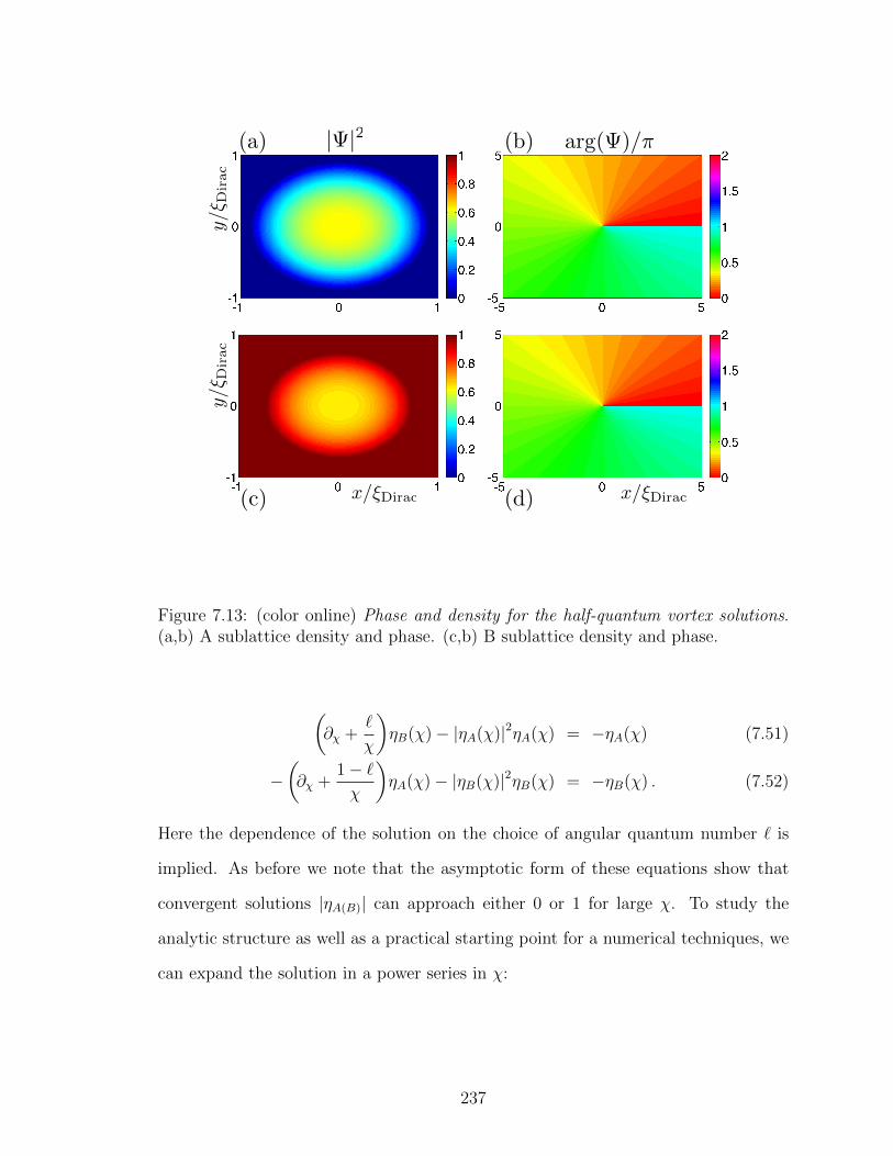
x/ξDiracx/ξDirac

y/ξ

Dirac

y/ξ D

irac

|Ψ|2 arg(Ψ)/π(a) (b)

(c) (d)

Figure 7.13: (color online) Phase and density for the half-quantum vortex solutions.(a,b) A sublattice density and phase. (c,b) B sublattice density and phase.

(∂χ +

`

χ

)ηB(χ)− |ηA(χ)|2ηA(χ) = −ηA(χ) (7.51)

−(∂χ +

1− `χ

)ηA(χ)− |ηB(χ)|2ηB(χ) = −ηB(χ) . (7.52)

Here the dependence of the solution on the choice of angular quantum number ` is

implied. As before we note that the asymptotic form of these equations show that

convergent solutions |ηA(B)| can approach either 0 or 1 for large χ. To study the

analytic structure as well as a practical starting point for a numerical techniques, we

can expand the solution in a power series in χ:

237

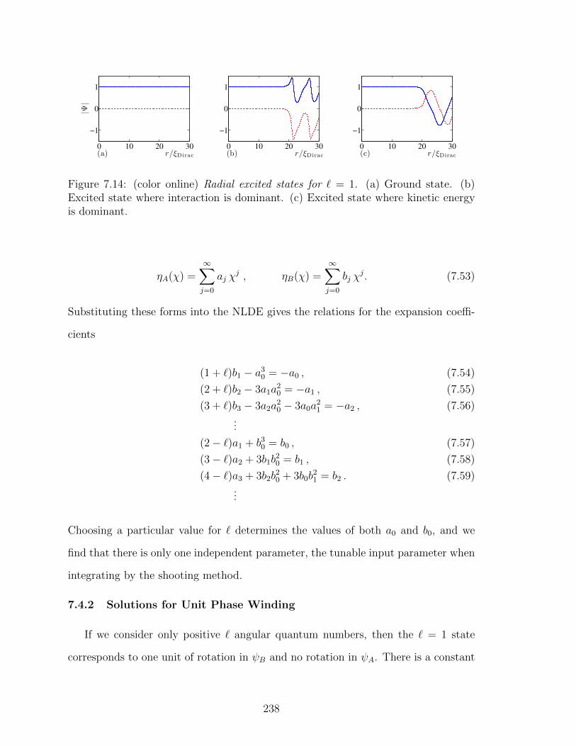
0 10 20 30

−1

0

1

(a) r/ξDirac

|Ψ|

0 10 20 30

−1

0

1

(b) r/ξDirac

0 10 20 30

−1

0

1

(c) r/ξDirac

Figure 7.14: (color online) Radial excited states for ` = 1. (a) Ground state. (b)Excited state where interaction is dominant. (c) Excited state where kinetic energyis dominant.

ηA(χ) =∞∑j=0

aj χj , ηB(χ) =

∞∑j=0

bj χj. (7.53)

Substituting these forms into the NLDE gives the relations for the expansion coeffi-

cients

(1 + `)b1 − a30 = −a0 , (7.54)

(2 + `)b2 − 3a1a20 = −a1 , (7.55)

(3 + `)b3 − 3a2a20 − 3a0a

21 = −a2 , (7.56)

...

(2− `)a1 + b30 = b0 , (7.57)

(3− `)a2 + 3b1b20 = b1 , (7.58)

(4− `)a3 + 3b2b20 + 3b0b

21 = b2 . (7.59)

...

Choosing a particular value for ` determines the values of both a0 and b0, and we

find that there is only one independent parameter, the tunable input parameter when

integrating by the shooting method.

7.4.2 Solutions for Unit Phase Winding

If we consider only positive ` angular quantum numbers, then the ` = 1 state

corresponds to one unit of rotation in ψB and no rotation in ψA. There is a constant

238

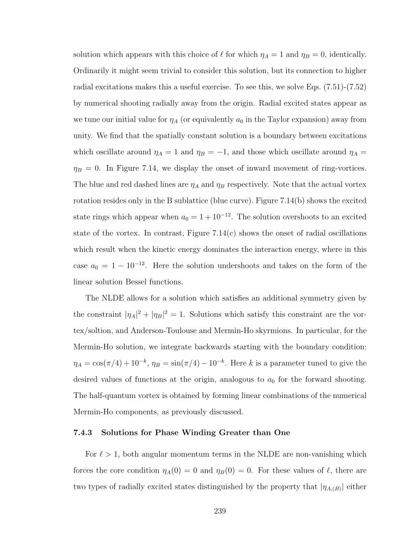
solution which appears with this choice of ` for which ηA = 1 and ηB = 0, identically.

Ordinarily it might seem trivial to consider this solution, but its connection to higher

radial excitations makes this a useful exercise. To see this, we solve Eqs. (7.51)-(7.52)

by numerical shooting radially away from the origin. Radial excited states appear as

we tune our initial value for ηA (or equivalently a0 in the Taylor expansion) away from

unity. We find that the spatially constant solution is a boundary between excitations

which oscillate around ηA = 1 and ηB = −1, and those which oscillate around ηA =

ηB = 0. In Figure 7.14, we display the onset of inward movement of ring-vortices.

The blue and red dashed lines are ηA and ηB respectively. Note that the actual vortex

rotation resides only in the B sublattice (blue curve). Figure 7.14(b) shows the excited

state rings which appear when a0 = 1 + 10−12. The solution overshoots to an excited

state of the vortex. In contrast, Figure 7.14(c) shows the onset of radial oscillations

which result when the kinetic energy dominates the interaction energy, where in this

case a0 = 1 − 10−12. Here the solution undershoots and takes on the form of the

linear solution Bessel functions.

The NLDE allows for a solution which satisfies an additional symmetry given by

the constraint |ηA|2 + |ηB|2 = 1. Solutions which satisfy this constraint are the vor-

tex/soltion, and Anderson-Toulouse and Mermin-Ho skyrmions. In particular, for the

Mermin-Ho solution, we integrate backwards starting with the boundary condition:

ηA = cos(π/4) + 10−k, ηB = sin(π/4)− 10−k. Here k is a parameter tuned to give the

desired values of functions at the origin, analogous to a0 for the forward shooting.

The half-quantum vortex is obtained by forming linear combinations of the numerical

Mermin-Ho components, as previously discussed.

7.4.3 Solutions for Phase Winding Greater than One

For ` > 1, both angular momentum terms in the NLDE are non-vanishing which

forces the core condition ηA(0) = 0 and ηB(0) = 0. For these values of `, there are

two types of radially excited states distinguished by the property that |ηA,(B)| either

239

0 5 10 15 20−1

0

1

2

(a)

|Ψ|

0 5 10 15 20−1

0

1

2

(b)0 5 10 15 20

−1

0

1

2

(c)

0 5 10 15 20−1

0

1

2

(d)

|Ψ|

0 5 10 15 20−1

0

1

2

(e)0 5 10 15 20

−1

0

1

2

(f )

0 5 10 15 20−1

0

1

2

(g) r/ξDirac

|Ψ|

0 5 10 15 20−1

0

1

2

(h) r/ξDirac

0 5 10 15 20−1

0

1

2

(i) r/ξDirac

Figure 7.15: (color online) Radial profiles for ` = 1 flat solution. (a)-(c) Dimensionlesschemical potential µ greater than 1. (d) µ equal to 1. (e)-(i) µ less than 1. In (a)the solution is most like the noninteracting solution µ > U , while the solution in (i)shows the strongly interacting case µ U .

oscillate around 1 or around 0.

7.4.4 Special Case of Zero Chemical Potential: Localized Ring-Vortices

To obtain these solutions we choose a particular rescaling of the NLDE which

allows us to take µ→ 0, so that

χ ≡ U2r/(~clµ), ηA ≡√µ/UfA, ηB ≡

õ/UfB. (7.60)

The resulting dimensionless NLDE is

−(∂χ +

`

χ

)ηB(χ) + |ηA(χ)|2ηA(χ) = µ2 ηA(χ) (7.61)(

∂χ +1− `χ

)ηA(χ) + |ηB(χ)|2ηB(χ) = µ2 ηB(χ) . (7.62)

240

For example, we look at the case ` = 1. We fix a0 = 1 and b0 = 0 in the Taylor

expansions and tune µ from unity toward zero. The progression for µ→ 0 is depicted

in the sequence of plots in Figure 7.15. As µ is reduced towards 1, oscillations about

ηA(B) ∼ 0 are pushed out towards large χ (a)-(c), flattening out the solution at

µ = 1 in (d). As µ is further reduced towards 0, oscillation nodes about ηA(B) ∼ 1

move inward from large χ and finally flatten out leaving only the ring-vortex feature

near χ = 0. An analogous sequence for arbitrary ` can be obtained. The difference

for ` < 1, is that since both components must vanish at the origin, we must take

b0, a0 = 0 but then specify the first derivative of ηA at the origin. We fix a0 = 0.001

in the Taylor expansion then tune µ as before. The vortex solutions with flat non-zero

asymptotic forms mark the point in the chemical potential parameter space where

kinetic and interaction terms of the NLDE are perfectly balanced. These form a

boundary between two solution regimes: one where the kinetic energy is dominant,

and the other where the interaction is dominant. The results also demonstrate how the

ring-vortex solutions smoothly connect to free Besssl solutions, with the topological

solutions as intermediate states.

7.4.5 Discrete Eigenvalue Spectra for Vortices in a Weak Harmonic Trap

Next, we study the same solutions as above but for the case of a highly oblate

harmonic confining potential, which defines the 2D system. In this case, the oscillator

frequencies satisfy ωz ω ≡ ωx, ωy. Since Eqs. (8.6)-(8.7) are already defined for a

2-dimensional system (the z-dependence has been integrated out), we require that the

harmonic potential be dependent only on the planar directions x and y. We then take

V (r) = (1/2)M ω2(x2 +y2)2 = (1/2)M ω2r2. We must choose a dimensional rescaling

of the NLDE appropriate to the harmonic oscillator. We divide through by the

harmonic oscillator energy ~ω and define the dimensionless variable and wavefunction

in terms of this energy scale:

241

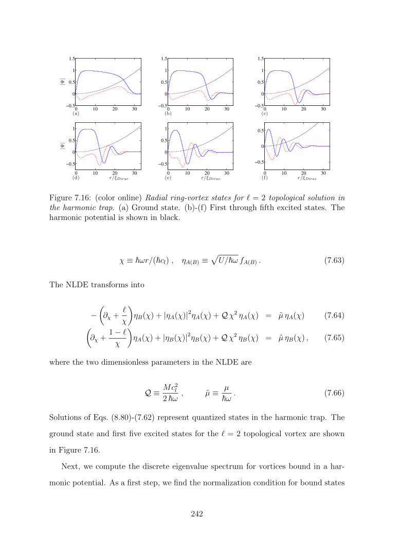
0 10 20 30−0.5

0

0.5

1

1.5

(a)

|Ψ|

0 10 20 30−0.5

0

0.5

1

1.5

(b) 0 10 20 30

−0.5

0

0.5

1

1.5

(c)

0 10 20 30

−0.5

0

0.5

1

(d) r/ξDirac

|Ψ|

0 10 20 30

−0.5

0

0.5

1

(e) r/ξDirac

0 10 20 30

−0.5

0

0.5

(f ) r/ξDirac

Figure 7.16: (color online) Radial ring-vortex states for ` = 2 topological solution inthe harmonic trap. (a) Ground state. (b)-(f) First through fifth excited states. Theharmonic potential is shown in black.

χ ≡ ~ωr/(~cl) , ηA(B) ≡√U/~ω fA(B) . (7.63)

The NLDE transforms into

−(∂χ +

`

χ

)ηB(χ) + |ηA(χ)|2ηA(χ) +Qχ2 ηA(χ) = µ ηA(χ) (7.64)(

∂χ +1− `χ

)ηA(χ) + |ηB(χ)|2ηB(χ) +Qχ2 ηB(χ) = µ ηB(χ) , (7.65)

where the two dimensionless parameters in the NLDE are

Q ≡ Mc2l

2 ~ω, µ ≡ µ

~ω. (7.66)

Solutions of Eqs. (8.80)-(7.62) represent quantized states in the harmonic trap. The

ground state and first five excited states for the ` = 2 topological vortex are shown

in Figure 7.16.

Next, we compute the discrete eigenvalue spectrum for vortices bound in a har-

monic potential. As a first step, we find the normalization condition for bound states

242

to be

∫χdχ(|ηA(χ)|2 + |ηB(χ)|2) = N , (7.67)

where the right hand side is given by

N =

√3 ~ωN U

3 t2h. (7.68)

To compute the spectra, we fixQ (which is the same as fixing ω and thus the oscillator

length) and vary µ, calculating the norm N for each value of µ. This gives the paired

values (N , µ). If in addition, we take the total number of particle N to be fixed, we

obtain an effective relation between the chemical potential µ and the interaction U .

The values for the free parameter in the Taylor expansion, a0, normalization N , and

corresponding chemical potential µ = µ/~ω, are tabulated in Table 7.3 for the radial

ground state of the ` = 2 topological vortex shown in Figure 7.16(a). Plots of this

data along with the spectra for other solutions are shown in Chapter 6. We have

taken Q = 0.001 for all of our calculations.

7.5 Relativistic Linear Stability Equations

Bogoliubov’s method was originally introduced in his 1947 paper [57] (see also [235,

236] for thorough contemporary treatments), and the concept later generalized by

Fetter [66] to accommodate nonuniform condensate profiles. The latter formulation

gives a convenient method for computing quasi-particle states and the associated

eigenvalues by simply substituting the spatial functions for a particular background

condensate into a pair of coupled differential equations, and then solving the resulting

eigenvalue problem. Fetter’s extended method was designed with a vortex profile

in mind, and has been proven successful in determining the stability of vortices in

trapped condensates as well as for gaining a deeper understanding of general vortex

dynamics [28, 29, 175]. The set of equations that we will derive in this section form

243

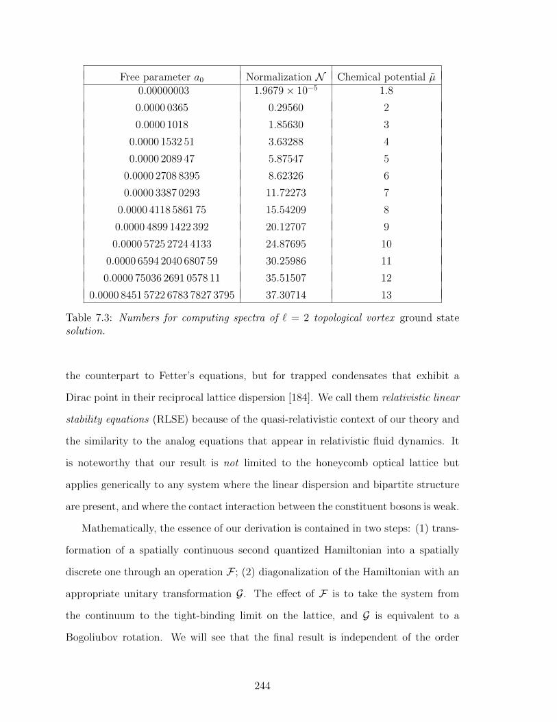
Free parameter a0 Normalization N Chemical potential µ0.00000003 1.9679× 10−5 1.8

0.0000 0365 0.29560 2

0.0000 1018 1.85630 3

0.0000 1532 51 3.63288 4

0.0000 2089 47 5.87547 5

0.0000 2708 8395 8.62326 6

0.0000 3387 0293 11.72273 7

0.0000 4118 5861 75 15.54209 8

0.0000 4899 1422 392 20.12707 9

0.0000 5725 2724 4133 24.87695 10

0.0000 6594 2040 6807 59 30.25986 11

0.0000 75036 2691 0578 11 35.51507 12

0.0000 8451 5722 6783 7827 3795 37.30714 13

Table 7.3: Numbers for computing spectra of ` = 2 topological vortex ground statesolution.

the counterpart to Fetter’s equations, but for trapped condensates that exhibit a

Dirac point in their reciprocal lattice dispersion [184]. We call them relativistic linear

stability equations (RLSE) because of the quasi-relativistic context of our theory and

the similarity to the analog equations that appear in relativistic fluid dynamics. It

is noteworthy that our result is not limited to the honeycomb optical lattice but

applies generically to any system where the linear dispersion and bipartite structure

are present, and where the contact interaction between the constituent bosons is weak.

Mathematically, the essence of our derivation is contained in two steps: (1) trans-

formation of a spatially continuous second quantized Hamiltonian into a spatially

discrete one through an operation F ; (2) diagonalization of the Hamiltonian with an

appropriate unitary transformation G. The effect of F is to take the system from

the continuum to the tight-binding limit on the lattice, and G is equivalent to a

Bogoliubov rotation. We will see that the final result is independent of the order

244

of these operations so that the full procedure can be summarized abstractly by the

commutative diagram

X −→ Y

↓ ↓ gY ′ −→ Z

f (7.69)

where X, Y, Y ′, and Z are the categories made up of the operator algebra A and

Hilbert space H of the theory at each step, e.g., X ≡ A ;H, and f and g are the

morphisms induced by the operations F and G.

7.5.1 Derivation

In deriving the RLSE we have relied fundamentally on Bogoliubov’s method [57] as

the underlying principle, and referred to Fetter’s work [66] for technical considerations

regarding nonuniform condensates. First, we recall the second-quantized many-body

Hamiltonian for weakly interacting bosons

H =

∫d2r ψ†H0ψ +

g

2

∫d2r ψ†ψ†ψψ , (7.70)

where, H0 ≡ − ~2

2m∇2 + V (r) . (7.71)

Here, V (r) is the lattice potential and g is the strength of the contact interaction. The

first step is to decompose the wavefunction as the sum ψ(r) = ζ(r) a0 + φ(r), where

we have split the wavefunction into a part that describes the condensate (first term)

and satisfies the bosonic commutation relation [a0 , a†0] = 1, and a second part that

describes the quasi-particle fluctuations. It is clear that the first term describes the

condensate since it destroys a particle in the mean field ζ, which, by itself, is a good

approximation to ψ. The second term destroys a particle in a number of single parti-

cle basis states of the noninteracting system and describes the part of ψ that deviates

245

from the mean field. Taking the Bogoliubov limit requires a0 → N1/20 , but we choose

to compute the commutator before taking this limit in order to retain the effect of the

presence of a macroscopic condensate field. We can obtain the commutation relations

for φ and φ† by knowing that ψ and ψ† obey commutation rules for bosons. We obtain

the quasi-particle commutation relations:[φ(r) , φ†(r′)

]= δ(r − r′) − ζ(r) ζ∗(r′),[

φ(r) , φ(r′)]

= 0,[φ†(r) , φ†(r′)

]= 0. In the Bogoliubov limit, the condensate wave-

function has no operator part in which case ψ may be written as ψ(r) = Ψ(r) + φ(r).

The condensate wavefunction has well defined phase and particle density and so may

be expressed as: Ψ(r) =√N0/A e

iS(r)√ρ(r), where A is the area covered by the pla-

nar condensate. Note that the radial part is normalized as A−1∫d2r ρ(r) = 1. With

these definitions, the usual bosonic commutation relations become:[φ(~r), φ†(r′)

]=

eiS(r) e−iS(r′) δ(r, r′), where δ(r, r′) = δ(r− r′)− A−1√ρ(r)

√ρ(r′).

Next, we transform to the new Hamiltonian defined by: K = H − µN = H −

µ∫d2r ψ† ψ, and we expand through second order in the operator part, eliminating

the linear terms by forcing the condensate wavefunction to satisfy the constraint:

(H0 − µ + g |Ψ|2)Ψ = 0. We arrive at the Bogoliubov Hamiltonian: K = K0 + K2,

wherein zero-order and second-order operator terms are grouped into K0 and K2

respectively. These are defined as

K0 =

∫d2rΨ∗(r)

[H0 − µ+

g

2|Ψ(r)|2

]Ψ(r) ,

K2 =

∫d2r φ†(r)

[H0 − µ+ 2g |Ψ(r)|2

]φ(r)

+g

2

∫d2r

[Ψ∗(r)]2 φ(r)φ(r) + φ†(r)φ†(r) [Ψ(r)]2

. (7.72)

Note that, in addition to the kinetic operator, we also have an arbitrary external

potential in the first two terms, which in our case will be the periodic potential

of the optical lattice. Eq.(7.72) is quadratic in the field operators and so may be

diagonalized with the appropriate field redefinition. To diagonalize Eq.(7.72), we first

246

apply the linear transformation: φ(r) = eiS(r)∑′

j

[uj(r) αj − v∗j (r) α†j

]and φ†(r) =

e−iS(r)∑′

j

[u∗j(r) α†j − vj(r) αj

], where the prime notation on the summation sign

indicates that we are omitting the condensate from the sum. The αj’s and α†j’s inherit

standard bosonic commutation relations from φ and φ†, and the spatially dependent

transformation coefficients uj(r) and vj(r) obey the completeness relations

′∑j

[uj(r) u∗j(r

′) − v∗j (r) vj(r′)]

= δ(r, r′) , (7.73)

′∑j

[uj(r) v∗j (r

′) − v∗j (r) uj(r′)]

= 0 , (7.74)

′∑j

[u∗j(r) vj(r

′) − vj(r) u∗j(r′)]

= 0 . (7.75)

So far, our discussion has taken place in two continuous spatial dimensions con-

strained only at the boundary by a trapping potential. We now want to translate to a

formalism that fits a two-dimensional periodic optical lattice potential with hexagonal

geometry. This is done by assuming a tight-binding limit at each lattice site. For-

mally, this corresponds to expanding the wavefunction in terms of a Wannier basis:

functions which are localized and centered on each lattice site. The nearest-neighbor

approximation then allows for a decomposition of the condensate and operator parts

in terms of individual sublattices labeled A and B. In this new basis, the spatial

dependence of the condensate and quasi-particle functions follows:

Ψ(r) =∑A

eik·(r−rA)√nAieiSAiw(r− rA)

+∑B

eik·(r−rB)√nBieiSBi w(r− rB), (7.76)

φ(r) = eiS(r)

′∑A,j

[uj,Ai

(r− rA)αj − v∗j,Ai(r− ~rA)α†j

]+eiS(r)

′∑B,j

[uj,Bi

(r− rB) βj − v∗j,Bi(r− rB)β†j

]. (7.77)

247

7.5.2 First Method - Tight-Binding Limit Followed by Diagonalization ofthe Quasi-Particle Hamiltonian

We substitute these expressions into the Hamiltonian then take the long-wavelength

limit, while translating the exponential (crystal) momentum factors to coincide with

the Dirac point. The continuum limit effectively converts the sublattice sums into

integrals. By performing one of the integrations, over the A sublattice, say, while

adhering to nearest neighbor overlaps, we obtain the affective Hamiltonian for the

condensate and quasi-particles: H = K0 + K2, where

K0 = (7.78)∫d2r

[i~cl ψ∗A(r)DψB(r) + i~ clψ∗B(r)D∗ψA(r) +

U

2|ψA(r)|4 +

U

2|ψB(r)|4

],

K2 =′∑

j,k

∫d2rαjβ

†k ~cl vj,AD∗v∗k,B + βjα

†k ~cl vj,B Dv∗k,A + 2U αjα

†k vj,A |ψA|2 v∗k,A

+ 2U βjβ†k vj,B |ψB|2 v∗k,B −

1

2U |ψA|2 αjα†k (uj,A v

∗k,A + u∗k,A vj,A)

− 1

2U |ψB|2 βjβ†k (uj,B v

∗k,B + u∗k,B vj,B) + α†jβk ~cl u∗j,AD∗uk,B

+ β†j αk ~cl u∗j,B Duk,A + 2U α†jαk u∗j,A |ψA|2 uk,A + 2U β†j βk u

∗j,B |ψB|2 uk,B

− 1

2U |ψA|2 α†jαk (v∗j,A uk,A + vk,A u

∗j,A)− 1

2U |ψB|2 β†j βk (v∗j,B uk,B + vk,B u

∗j,B)

− αjβk ~cl vj,AD∗uk,B − βjαk ~cl vj,B Duk,A − 2Uαjαk vj,A |ψA|2 uk,A− 2U βjβk vj,B |ψB|2 uk,B +

1

2U |ψA|2 αjαk(uj,A uk,A + vk,A vj,A)

+1

2U |ψB|2 βjβk (uj,B uk,B + vk,B vj,B) − α†jβ

†k~cl u

∗j,AD∗v∗k,B

− ~cl β†j α†k u∗j,B Dv∗k,A − 2U α†jα

†k u∗j,A |ψA|2 v∗k,A − 2U β†j β

†k u∗j,B |ψB|2 v∗k,B

+1

2U |ψA|2 α†jα†k (u∗j,A u

∗k,A + v∗k,A v

∗j,A)

+1

2U |ψB|2 β†j β†k (u∗j,B u

∗k,B + v∗k,B v

∗j,B)

. (7.79)

Note that we have defined the condensate two-spinor in terms of the A and B sublat-

tice components: Ψ(r) = [ψA(r), ψB(r)]T . Next, we isolate the first six terms (terms

248

with the daggered operator to the right) and write them as a matrix contraction of

two pure operator valued vectors,

(αj , βj

) ( Au,v DA,B

DB,A Bu,v

) (α†kβ†k

), (7.80)

where

Au,v ≡ 2Uvj,A |ψA|2 v∗k,A −1

2U |ψA|2 (uj,Av

∗k,A + u∗k,Avj,A) , (7.81)

Bu,v ≡ 2Uvj,B |ψB|2 v∗k,B −1

2U |ψB|2 (uj,Bv

∗k,B + u∗k,Bvj,B) , (7.82)

DA,B ≡ ~clvj,AD∗v∗k,B , (7.83)

DB,A ≡ ~clvj,BD v∗k,A . (7.84)

The eigenvalues are then obtained by

det

(Au,v − λ DA,B

DB,A Bu,v − λ

)= 0 (7.85)

⇒(Au,v − λ) (Bu,v − λ) − DA,BDB,A = 0 , (7.86)

λ± =(Au,v + Bu,v)

2± 1

2

√(Au,v − Bu,v) + 4DA,BDB,A , (7.87)

and the corresponding eigenvectors follow:

~V± =

(1

DB,A

(λ±−Bu,v)

). (7.88)

The unitary matrix that diagonalizes Eq.(7.80) is

U =1√2

(1 1

DB,A

(λ+−Bu,v)

DB,A

(λ−−Bu,v)

). (7.89)

The first six terms in Eq. (7.79) may be expressed in the new basis as

λ+jk c+,j c†+,k + λ−jk c−,j c

†−,k , (7.90)

249

where we have included the j, k subscripts on the eigenvalues to be fully descriptive.

The new quasi-particle operators can be written in terms of the old ones as

c†±,j =1√2

[α†j +

D∗B,A(λ∗±jk − B∗u,v)

β†j

]. (7.91)

Note that the right hand side is k-dependent which is implied on the left. The

substance of the transformation is contained in the momentum and space-dependent

eigenvalues

λ±jk = Uvj,A |ψA|2 v∗k,A −1

4U |ψA|2 (uj,Av

∗k,A + u∗k,Avj,A) + Uvj,B |ψB|2 v∗k,B

− 1

4U |ψB|2 (uj,Bv

∗k,B + u∗k,Bvj,B)

±[

Uvj,A |ψA|2 v∗k,A −1

4U |ψA|2 (uj,Av

∗k,A + u∗k,Avj,A) (7.92)

−Uvj,B |ψB|2 v∗k,B +1

4U |ψB|2 (uj,Bv

∗k,B + u∗k,Bvj,B)

]2

+ (~cl)2 vj,A(D∗v∗k,B)vj,B(Dv∗k,A)1/2

. (7.93)

The next step is to constrain the quasi-particle amplitudes in Eq. (7.93) (the u’s and

v’s) in order to diagonalize the Hamiltonian with respect to the momentum indices j

and k. First, we let

~clvj,AD∗v∗k,B = 2Uvj,A |ψA|2 v∗k,A −1

2U |ψA|2 (uj,Av

∗k,A + u∗k,Avj,A)

~clvj,B D v∗k,A = 2Uvj,B |ψB|2 v∗k,B −1

2U |ψB|2 (uj,Bv

∗k,B + u∗k,Bvj,B) , (7.94)

and then substitute these into Eq.(7.93), which reduces the two eigenvalues to

250

λ+jk = −µ vj,A v∗k,A + 2U vj,A |ψA|2 v∗k,A−1

2U |ψA|2 (uj,A v

∗k,A + u∗k,A vj,A)

−µ vj,B v∗k,B + 2U vj,B |ψB|2 v∗k,B−1

2U |ψB|2 (uj,B v

∗k,B + u∗k,B vj,B)

and ,

λ−jk = 0 , (7.95)

where we have reinserted the chemical potential terms. It is important that Eqs. (7.94)

depend only on one index so that quasi-particle amplitudes for different eigeneneregies

are not coupled. Dividing Eqs. (7.94) through by vj,A and vj,B, respectively, cancels

all j-index terms except for ones that appear as uj,A/vj,A and uj,B/vj,B. To completely

decouple the j-k modes, we must ensure that uj,A/vj,A = uj,B/vj,B = η(~r ), i.e., the

amplitudes for any given quasi-particle mode have the same relative spatial form. We

can then rewrite λ+jk as

λ+jk =1

2~cl vj,AD∗v∗k,B −

1

2µ vj,A v

∗k,A

+Uvj,A |ψA|2 v∗k,A −1

4U |ψA|2 (uj,Av

∗k,A + u∗k,Avj,A)

+1

2~cl vj,B D v∗k,A −

1

2µ vj,B v

∗k,B

+Uvj,B |ψB|2 v∗k,B −1

4U |ψB|2 (uj,Bv

∗k,B + u∗k,Bvj,B) . (7.96)

Finally, we impose the constraints

− 1

4Ekv

∗k,A =

1

4~clD∗v∗k,B −

1

4µv∗k,A +

1

2U |ψA|2 v∗k,A −

1

4U |ψA|2 u∗k,A (7.97)

−1

4Ejvj,A =

1

4~clD∗vj,B −

1

4µvj,A +

1

2U |ψA|2 vj,A −

1

4U |ψA|2 uj,A . (7.98)

Multiplying Eqs. (7.97) and (7.98) by vj,A and v∗k,A, respectively, and using the prop-

erty that∫d2r vj,B D v∗k,A =

∫d2r(D∗vj,B) v∗k,A , we may separate out 1/2 of each

derivative term in Eq. (7.96), which reduces the non-derivative terms in the first line

251

of Eq. (7.96) to

−1

4(Ek + Ej) v

∗k,A vj,A . (7.99)

We may reduce the second line using the other half of each derivative term, thereby

condensing the eigenvalues down to

λ+jk = −1

4(Ek + Ej) (v∗k,A vj,A + v∗k,B vj,B) . (7.100)

The next six terms in Eq.(7.79) may be diagonalized in a similar way yielding the

eigenvalues

λ+jk = −µu∗j,A uk,A + 2U u∗j,A |ψA|2 uk,A−1

2U |ψA|2 (v∗j,A uk,A + vk,A u

∗j,A)

−µu∗j,B uk,B + 2U u∗j,B |ψB|2 uk,B−1

2U |ψB|2 (v∗j,B uk,B + vk,B u

∗j,B)

and ,

λ−jk = 0 . (7.101)

Following our previous steps, we obtain

λ+jk =1

4(Ek + Ej) (u∗k,A uj,A + u∗k,B uj,B) . (7.102)

Combining Eqs. (7.100) and (7.102), and inserting the quasi-particle operators, re-

duces the first twelve terms in Eq. (7.79) to the expression

1

4

′∑j,k

∫d2r (Ej + Ek)

[c†+,j c+,k (u∗k,A uj,A + u∗k,B uj,B)− c+,j c

†+,k (v∗k,A vj,A + v∗k,B vj,B)

].

(7.103)

For the special case where j = k, we may further combine the terms at the cost of

an extra c-number term to arrive at

252

−1

2

′∑k

∫d2r 2Ek(v

∗k,Avk,A + v∗k,Bvk,B)

+1

4

′∑j,k

∫d2r(Ej + Ek)c

†+,j c+,k(u

∗k,Auj,A − v∗k,Avj,A

+u∗k,Buj,B − v∗k,Bvj,B). (7.104)

Applying the completeness relations∫d2r (u∗k,A uj,A−v∗k,A vj,A) = δi,j and

∫d2r (u∗k,B uj,B−

v∗k,A vj,B) = δi,j, contracts Eq. (7.104) down to

−′∑

k

∫d2r Ek (|vk,A|2 + |vk,B|2) +

′∑k

Ek c†+,kc+,k. (7.105)

Diagonalizing the rest of Eq.(7.79) (terms with no daggered operators and ones

with only daggered operators) by capitalizing on the j-k symmetry of terms such

as∫d2r uk,A vj,A, and anti-symmetry of the (Ej − Ek) factor, we obtain the final form

of the interacting Hamiltonian

H =

∫d2r [i~cl ψ∗A(r)(∂x + i∂y)ψB(r) + i~cl ψ∗B(r)(∂x − i∂y)ψA(r)

+U

2|ψA(r)|4 +

U

2|ψB(r)|4

]−

′∑j

Ej

∫d2r vT∗j vj +

′∑j

Ej c†+, j c+, j , (7.106)

with the resulting constraints on quasi-particle amplitudes given by

i ~clD∗uj,B − µuj,A + 2U |ψA|2 uj,A − U |ψA|2 vj,A = Ejuj,A , (7.107)

i ~clD uj,A − µuj,B + 2U |ψB|2 uj,B − U |ψB|2 vj,B = Ejuj,B , (7.108)

i ~clD vj,B − µvj,A + 2U |ψA|2 vj,A − U |ψA|2 uj,A = −Ejvj,A , (7.109)

i ~clD∗vj,A − µvj,B + 2U |ψB|2 vj,B − U |ψB|2 uj,B = −Ejvj,B . (7.110)

7.5.3 Second Method - Diagonalize the Quasi-Particle Hamiltonian thenImpose Tight-Binding

Although the first method is cumbersome, it is the more rigorous approach and

instills confidence in the final constraint equations. A shorter approach is to first

253

obtain the usual Bogoliubov equations for a condensate not confined in a lattice, and

then apply the tight-binding limit directly. The Bogoliubov Hamiltonian is

H =

∫d2rΨ∗(r)

[H0 − µ+

g

2|Ψ(r)|2

]Ψ(r)

−′∑

j

Ej

∫d2r |vj(~r)|2 +

′∑j

Ejα†jαj , (7.111)

with the constraint equations (BdGE) given by

Luj − g |Ψ|2 vj = Ejuj (7.112)

L∗ vj − g |Ψ|2 uj = −Ejvj . (7.113)

In Eqs. (7.112)-(7.113), L is a differential operator which combines terms that couple

the quasi-particle and condensate velocities. An additional implicit constraint is

that Ψ satisfies the nonlinear Schrodinger equation. To pass to the tight-binding

limit, we express all spatial functions in Eqs. (7.111)-(7.113) in terms of Wannier

functions for the individual sublattices, and evaluate the Bloch plane wave factors at

the Dirac point momemtum. Adhering to nearest-neighbor overlap for on-site Wannier

functions, we integrate out spatial degrees of freedom (which splits the honeycomb

lattice into A and B sublattices), regroup terms into finite differences, and then take

the continuum limit. Eq. (7.111) then transforms to Eq. (7.106), while Eqs. (7.112)-

(7.113) transform to Eqs. (7.107)-(7.110) with several additional derivative terms

contained in L as follows

− ~2

2m

[∇2 + i∇2φ+ 2i∇φ · ∇ − (∇φ)2

]uj , (7.114)

where φ is the condensate phase. After going through the steps that culminate in the

tight-binding continuum limit, these terms transform to

i~clD∗uk,B(A) +[−i~τ1∇φA(B) · ∇+ ~τ2|∇φA(B)| − i~τ3(∇2φA(B))

]uk,A(B) ,(7.115)

254

where the coefficients encapsulate the spatial integrals as follows: τ1∝ |∫drw∗A∇wB|,

τ2∝ |∫drw∗A(∇φ)wA|, τ3∝

∫drw∗A|∇φ|2wA. These extra terms depend on the con-

densate phase φA(B), and so couple the superfluid velocity to the quasi-particle ex-

citations. In particular, the term with coefficient τ1 depends on the direction of

quasi-particle emission relative to the motion of the condensate. The relativistic lin-

ear stability equations, Eqs. (7.107)-(7.110), may be expressed in compact notation

as

Duk − UΨvk = Ekuk, (7.116)

D∗vk − UΨuk = −Ekvk , (7.117)

where

Ψ ≡ diag(|ψA|2 , |ψB|2), (7.118)

Ek ≡ diag(Ek, Ek), (7.119)

[D ]1,1 ≡ −µ+ 2U |ψA|2 − i~τ1∇φA · ∇+~τ2 |∇φA| − i~τ3

(∇2φA

), (7.120)

[D ]2,2 ≡ −µ+ 2U |ψB|2 − i~τ1∇φB · ∇+~τ2 |∇φB| − i~τ3

(∇2φB

), (7.121)

[D ]1,2 = [D ]∗2,1 ≡ i~clD∗. (7.122)

7.5.4 Proof of NLDE Limit to NLSE

The standard Dirac equation has a well defined non-relativistic limit to the Schrodinger

equation. The proof uses the fact that, in the low energy limit, the mass term (the

term multiplied by mc2) is the largest contribution to the energy. One spinor equation

is back-substituted into the remaining equation and the approximation reduces this

down to an expression that has the correct Schrodinger kinetic term. It is natural to

ask if there exists some limit in which our nonlinear Dirac equation reduces to the

nonlinear Schrodinger equation, and, if so, how to tune the parameters in order to

observe this transition in the laboratory. To show that the NLDE can be reduced to

255

the NLSE, we start from the discrete nonlinear Dirac equation for one Dirac point,

which is an intermediate step in deriving the NLDE:

−th(ψBj

eik·δ3 + ψBj−n1eik·δ1 + ψBj−n2

eik·δ2)− t0ψAj

+ U∣∣ψAj

∣∣2 ψAj= 0 ,(7.123)

−th(ψAj

e−ik·δ3 + ψAj+n1e−ik·δ1 + ψAj+n2

e−ik·δ2)− t0ψBj

+ U∣∣ψBj

∣∣2 ψBj= 0 .(7.124)

Physically, th, t0, U , and k are the hopping, same site, and on-site interaction energies

and crystal momentum, respectively. The δ’s, n’s, and 2D vector indices j are the

lattice vectors described in our original derivation [52]. For weak interactions, we

can make the on-site energy much larger than the contact interaction strength by

adjusting the lattice potential so that |t0| U . After inserting the correct values for

the lattice vectors and solving Eq. (7.124) for ψBj, to lowest order in U/t0, we obtain

ψBj=

th−t0

(ψAj

+ ψAj+n1ei2π/3 + ψAj+n2

e−i2π/3). (7.125)

From Eq. (7.125) we may write down the corresponding expressions for neighboring

sites by shifting the indices using the lattice vectors nj:

ψBj−n1=

th−t0

[ψAj−n1

+ ψAjei2π/3 + ψAj+(n2−n1)

e−i2π/3]

(7.126)

ψBj−n2=

th−t0

[ψAj−n2

+ ψAj−(n2−n1)ei2π/3 + ψAj

e−i2π/3]. (7.127)

Substituting Eqs. (7.125)-(7.127) into Eq. (7.123), expanding complex factors and

regrouping the terms to form finite differences, we arrive at the expression

t2h2t0(ψj+n1 − 2ψj + ψj−n1) + (ψj+n2 − 2ψj + ψj−n2)

+(ψj+(n2−n1) − 2ψj + ψj−(n2−n1) )

−i√

3 [(ψj+n1 − ψj) + (ψj − ψj−n1)− (ψj+n2 − ψj)− (ψj − ψj−n2) +

(ψj+(n2−n1) − ψj

)+(ψj − ψj−(n2−n1)

)]− t0ψj + U |ψj|2 ψj = 0 . (7.128)

256

It is somewhat surprising that this is a version of the discrete nonlinear Schrodinger

equation for the honeycomb lattice in the sense that, in the continuum limit, it gives

the usual nonlinear Schrodinger equation with cubic nonlinearity. Substituting the

correct continuum limit forms for the finite differences and then expressing the result

in x− y coordinates:

t2ha2

2t0

[(3

4

∂2

∂x2+

1

4

∂2

∂y2−√

3

2∂x∂y

)ψ +

(3

4

∂2

∂x2+

1

4

∂2

∂y2+

√3

2∂x∂y

)ψ +

∂2ψ

∂y2

−i√

3

a

(√3∂ψ

∂x− ∂ψ

∂y−√

3∂ψ

∂x− ∂ψ

∂y+ 2

∂ψ

∂y

)]− t0ψ + U |ψ|2 ψ = 0 , (7.129)

which finally reduces to

t2h~2a2

2t0

(∂2ψ

∂x2+∂2ψ

∂y2

)− t0 ψ + U |ψ|2 ψ = 0 . (7.130)

This is the time-independent nonlinear Schrodinger equation. Note that we have

reintroduced the correct number of factors of ~ and the lattice constant a. By defining

the effective mass and chemical potential as

Meff = − t0t2ha

2, µ = t0 , (7.131)

we may write Eq. (7.130) in the more familiar form

− ~2

2m∇2ψ − µψ + U |ψ|2 ψ = 0 . (7.132)

7.5.5 Proof of RLSE limit to BdGE

For states with energies that are large measured from the Dirac point (deviations

from the linear theory), we expect the relativistic formalism to no longer be appropri-

ate and expect to recover a non-relativistic Schrodinger framework for quasi-particle

dynamics. Based on our discussion in Sec. 7.3, we expect to find an analogous mapping

between the RLSE and the BdGE. This is indeed possible and easy to demonstrate

257

by writing the RLSE in discrete form similar to the method we used to show the

connection between the NLDE and NLSE, i.e., by manipulating the discrete version

of Eqs. (7.107)-(7.110) followed by taking the continuum limit. Grouping the equa-

tions pairwise, solving Eq. (7.108) for uj,B, and back-substituting into Eq. (7.107),

we arrive at an intermediate form where the Dirac kinetic term D has been converted

to the Schrodinger ∇2 form. To complete the reduction, we require the following

approximation. At each lattice site, the chemical potential µ is made up of contribu-

tions from H0 (kinetic and lattice potential energy) and from the contact interaction

energy U . If the lattice potential is deep and the interaction weak, then the con-

tribution from H0 dominates the chemical potential, and we find µ ≈ −t0 where t0

is a self energy. If we then examine the regime where µ U, ∇φA(B), Ek, we see

that the factor multiplying the ∇2 term appears as −t2h~2a2/2t0, where th, t0, and a

are the hopping energy, self energy, and lattice constant, respectively. We are then

free to read off the effective quasi-particle mass as meff = t0/t2ha

2. Performing the

same algebraic steps with Eqs. (7.109)-7.110), and using the same approximations,

completes the reduction of the RLSE to the BdGE.

7.6 Stability of Vortex Solutions

Having obtained the RLSE by two different methods, and in light of the nat-

ural mapping that we found between these and the BdGE, we are confident that

Eqs. (7.116)-(7.117) give us the correct way to compute the low-energy structure

(quasi-particle states and eigenenergies) for any of the solutions in Sec. 7.3. The

most immediate and pragmatic concern is the combined effect of the honeycomb lat-

tice geometry and the inter-particle interaction on the lifetime of a vortex state. It

should be emphasized that the presence of an infinite tower of negative energy states

below the Dirac point seems to imply that a condensate residing there will eventually

decay provided there is a mechanism for energy dissipation into noncondensate modes

(i.e., secondary interactions with thermal atoms). Generically, negative energy states

258

are present for moving condensates for which excitations subtended by a backward

cone have negative frequencies [66]. Moreover, when a vortex is present, small dis-

placements of the core from the symmetry axis of the trap results in a precession of

the core, which, when combined with dissipation, causes the vortex to spiral to the

edge of the condensate. In the case of zero-lattice potential, this dynamical process

is known to be driven by the anomalous modes in the linear spectrum (modes with

negative energy and positive norm) [175]. The time for a vortex to spiral to the edge

of the trap would then define its lifetime. We note that, in our case, this precessional

motion is most likely canceled by introducing rotation to the trap as in the ordinary

case with no lattice [29, 175].

To undertake a full treatment of the lifetime would mean computing this spiraling

time and then comparing it with the lifetime that we compute here due to the dynam-

ical instability from the complex frequencies. The lifetime of the vortex would then

be the smaller of the two values. Nevertheless, in cases where dissipation is weak and

the vortex is centered on the symmetry axis of the trap, the dominant source of insta-

bility arises from the complex eigenvalues in the solution of the RLSE. We will limit

our analysis to the effect of the latter, and regard the negative, real, part of the eigen-

values from a standpoint of metastability. Physically, the complex eigenvalue gives

rise to fluctuations in the angular rotation of the vortex spinor components [184]. In

the case of the NLDE, this is a result of internal “friction” between the two spinor

components displayed in the complex derivative terms of the Dirac kinetic energy.

This drag force between the two vortex components (or between vortex and soliton)

eventually causes substantial depletion of the condensate. This is the measure that

we will use to compute vortex lifetimes.

7.6.1 Solving the RLSE

To determine stability of our vortex solutions, we expand Eqs. (7.116)-(7.117) and

express them in plane-polar coordinates, factor the quasi-particle amplitudes into ra-

259

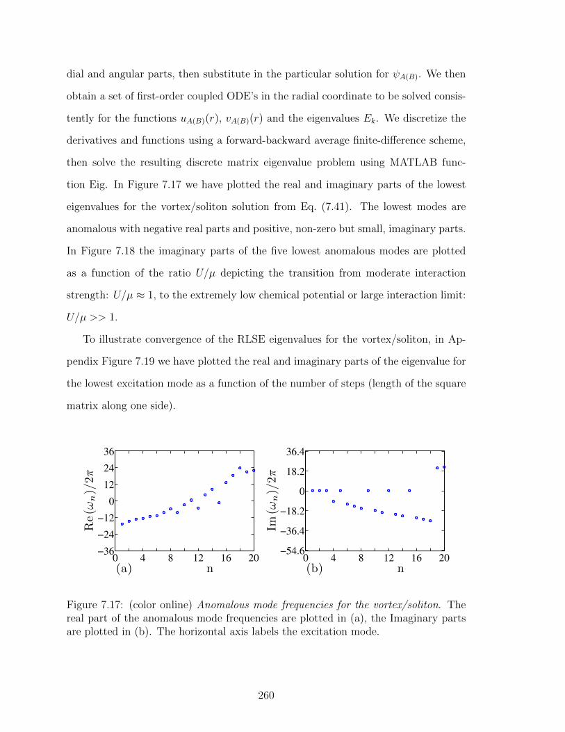
dial and angular parts, then substitute in the particular solution for ψA(B). We then

obtain a set of first-order coupled ODE’s in the radial coordinate to be solved consis-

tently for the functions uA(B)(r), vA(B)(r) and the eigenvalues Ek. We discretize the

derivatives and functions using a forward-backward average finite-difference scheme,

then solve the resulting discrete matrix eigenvalue problem using MATLAB func-

tion Eig. In Figure 7.17 we have plotted the real and imaginary parts of the lowest

eigenvalues for the vortex/soliton solution from Eq. (7.41). The lowest modes are

anomalous with negative real parts and positive, non-zero but small, imaginary parts.

In Figure 7.18 the imaginary parts of the five lowest anomalous modes are plotted

as a function of the ratio U/µ depicting the transition from moderate interaction

strength: U/µ ≈ 1, to the extremely low chemical potential or large interaction limit:

U/µ >> 1.

To illustrate convergence of the RLSE eigenvalues for the vortex/soliton, in Ap-

pendix Figure 7.19 we have plotted the real and imaginary parts of the eigenvalue for

the lowest excitation mode as a function of the number of steps (length of the square

matrix along one side).

0 4 8 12 16 20−36

−24

−12

0

12

24

36

(a) n

Re(ω

n)/2π

0 4 8 12 16 20−54.6

−36.4

−18.2

0

18.2

36.4

(b) n

Im(ω

n)/2π

Figure 7.17: (color online) Anomalous mode frequencies for the vortex/soliton. Thereal part of the anomalous mode frequencies are plotted in (a), the Imaginary partsare plotted in (b). The horizontal axis labels the excitation mode.

260

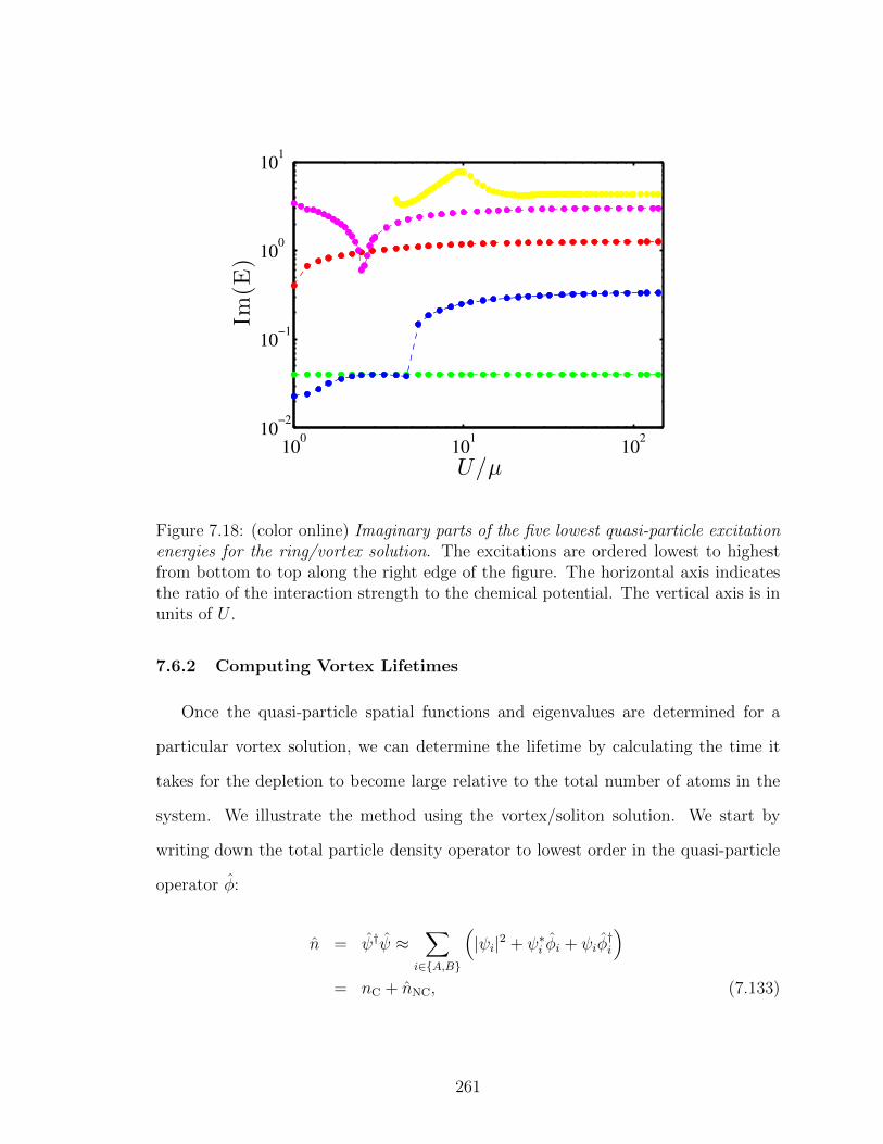
100

101

102

10−2

10−1

100

101

U/µ

Im(E

)

Figure 7.18: (color online) Imaginary parts of the five lowest quasi-particle excitationenergies for the ring/vortex solution. The excitations are ordered lowest to highestfrom bottom to top along the right edge of the figure. The horizontal axis indicatesthe ratio of the interaction strength to the chemical potential. The vertical axis is inunits of U .

7.6.2 Computing Vortex Lifetimes

Once the quasi-particle spatial functions and eigenvalues are determined for a

particular vortex solution, we can determine the lifetime by calculating the time it

takes for the depletion to become large relative to the total number of atoms in the

system. We illustrate the method using the vortex/soliton solution. We start by

writing down the total particle density operator to lowest order in the quasi-particle

operator φ:

n = ψ†ψ ≈∑

i∈A,B

(|ψi|2 + ψ∗i φi + ψiφ

†i

)= nC + nNC, (7.133)

261

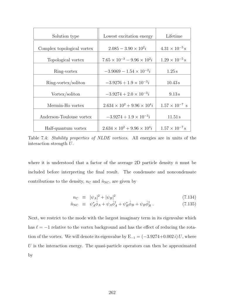
Solution type Lowest excitation energy Lifetime

Complex topological vortex 2.085− 3.90× 102i 4.31× 10−5 s

Topological vortex 7.65× 10−3 − 9.96× 102i 1.29× 10−5 s

Ring-vortex −3.9069− 1.54× 10−2i 1.25 s

Ring-vortex/soliton −3.9276 + 1.9× 10−3i 10.43 s

Vortex/soliton −3.9274 + 2.0× 10−3i 9.13 s

Mermin-Ho vortex 2.634× 102 + 9.96× 104i 1.57× 10−7 s

Anderson-Toulouse vortex −3.9274 + 1.9× 10−3i 11.51 s

Half-quantum vortex 2.634× 102 + 9.96× 104i 1.57× 10−7 s

Table 7.4: Stability properties of NLDE vortices. All energies are in units of theinteraction strength U .

where it is understood that a factor of the average 2D particle density n must be

included before interpreting the final result. The condensate and noncondensate

contributions to the density, nC and nNC, are given by

nC ≡ |ψA|2 + |ψB|2 (7.134)

nNC ≡ ψ∗AφA + ψAφ†A + ψ∗BφB + ψBφ

†B . (7.135)

Next, we restrict to the mode with the largest imaginary term in its eigenvalue which

has ` = −1 relative to the vortex background and has the effect of reducing the rota-

tion of the vortex. We will denote its eigenvalue by E−1 = (−3.9274+0.002 i)U , where

U is the interaction energy. The quasi-particle operators can then be approximated

by

262

φA,−1(r, θ, t) ≈ e−iE−1t/~ uA,−1(r) αj + eiE−1t/~ v∗A,−1(r) α†j (7.136)

φB,−1(r, θ, t) ≈ e−iE−1t/~ uB,−1(r) βj + eiE−1t/~ v∗B,−1(r) β†j . (7.137)

Notice that these expressions do not depend on the polar angle because we are in the

rotating frame of the vortex. We recall that the spatial functions have the properties

uA,−1(r), uB,−1(r) ∼ 10−2 and vA,−1(r), vB,−1(r) ∼ 10−5 [184], where all are peaked

in the “notch” region ξDirac < r < 2ξDirac, and where the absolute values of the slopes

of the soliton and vortex are maximum. In this region, the normalization integrals

(one for each sublattice) are given by

∫d2r

[|uA(B),−1(r)|2 − |vA(B),−1(r)|2

]> 0 . (7.138)

This combination of positive norm and negative Re(E−1) signals the presence of the

anomalous mode. Next, we fix the total number of particles N of the system and take

all N particles to be in the condensate at t = 0. We can then compute the depletion

out of the vortex/soliton state as a function of time,

NNC,vs(t) = n

∫d2r [〈nα||nNC,vs||0〉+ |〈nβ||nNC,vs||0〉] , (7.139)

where |0〉 and |nα(β)〉 are the initial and final A(B) sublattice quasi-particle number

states, respectively. Retaining only the terms which grow exponentially in time, and

using the fact that the vA(B) terms are three orders of magnitude smaller than the

uA(B) terms, Eq. (7.139) reduces to

NNC,vs(t) = eIm(E−1)t/~ 2π n

∫ 10ξDirac

0

rdr[(r/ξDirac)uA,−1(r) + uB,−1(r)]√

1 + (r/ξDirac)2, (7.140)

where we have inserted spatial dependence of the vortex/soliton and taken the size of

the condensate to be equal to ten times the healing length. To compute the lifetime

τvs, we can determine the time it takes for the depletion number to grow to roughly

263

the number of atoms initially in the condensate. Thus, we set Eq. (7.140) equal to∫d2r n for time t equal to the lifetime τvs, which gives

τvs =~

Im(E−1)ln (50/I) =

~(0.002)U

ln (50/I) . (7.141)

The dimensionless integral I contains the overlap of the vortex background with the

quasi-particle functions and measures the nonuniformity of particle being ejected from

the condensate:

I ≡ (π102)−1/2

∫ 10

0

r′dr′ [r′uA,−1(r′) + uB,−1(r′)] /√

1 + r′2 . (7.142)

Note the insertion of the normalization factor for the wavefunction (π102)−1/2. Eval-

uating the integral numerically gives I ≈ 0.0065. Using the values for parameters

in Table 7.1, we find the lifetime of the vortex/soliton state to be: τvs = 9.13 s. We

have computed lifetimes for all of our solutions and listed them in Table 7.4.

7.7 Conclusion

We have found eight different types of vortex solutions to the NLDE using asymp-

totic, numerical, and analytical methods in addition to performing a detailed analysis

of their lifetimes, elucidating the low-energy landscape for these solutions. Vortex

lifetimes were computed based on dynamical instabilities induced by quantum fluc-

tuations: complex eigenvalues appear in the linear spectrum for all vortex types as

a result of the couplings between spinor components through Dirac derivative terms.

Nevertheless, for four of our solutions, the imaginary parts are smaller than the in-

teraction energy by several orders of magnitude resulting in experimentally realistic

lifetimes of about ten seconds.

In the experimental part of our paper, we have provided a clear path towards

realizing relativistic vortices in the laboratory: detailed instructions on lattice con-

struction, condensation of bosons at both K and K′ points, and a method for creating

264

relativistic vortices are explained using established experimental techniques. Impor-

tantly, our proposed method for populating the Dirac points by laser assisted Bragg

scattering provides a dynamically stable approach by maintaining a zero group veloc-

ity for the condensate. We have discussed specific conditions for energy, density, in-

teraction strength, and lattice depth for observing a transition from the NLDE/RLSE

regime to that of the NLSE/BdGE. The density profiles of our solutions should be

observable by the usual time-of-flight techniques used to detect Dirac fermions in the

laboratory [15, 133].

Interesting new problems naturally arise given the interdisciplinary nature of our

work. The following are a few examples. First, the study of nonlinear partial differ-

ential equations provides an extensive array of techniques for probing, solving, and

classifying equations which could be used for a more complete investigation of the

NLDE. Second, by including rotation, one would expect a qualitative change in the

anomalous mode structure as a function of trap rotation speed. In the future, we plan

to generalize our analysis to the case of a rotating trap in analogy to ordinary trapped

BECs in the absence of a lattice. This would provide a more complete understanding

of relativistic vortex stabilities and their relationship to ordinary single and multi-

component vortices. Third, our solutions suggest a possible mapping to vortices in

Chern-Simons theory [237–239]. This seems to indicate a deeper connection between

the NLDE and high energy models which could lead to cold atomic simulations of

more exotic relativistic field theories. Finally, our results should be easily reproduced

within an optics setting by adhering to the momentum space bounds we have pro-

vided, thus contributing to the long-standing mutual exchange between condensed

matter and nonlinear optics.

Acknowledgments

265

This material is based in part upon work supported by the National Science Foun-

dation under grant numbers PHY-1067973, PHY-1011156, and the Air Force Office

of Scientific Research grant number FA9550-08-1-0069. L.D.C. thanks the Alexan-

der von Humboldt foundation and the Heidelberg Center for Quantum Dynamics for

additional support.

7.8 Appendix A: Convergence of Numerical Solutions of the NLDE andRLSE

We show convergence of the numerical solutions of the NLDE by looking at the

l = 2 ring-vortex solution. To obtain the solution, we use a simple forward-difference

scheme to discretize the radial derivatives in Eqs. (8.6)-(8.7) and then integrate out

from the core of the vortex with the following values for the parameters: µ/U =

1, fA(0) = 10−4. The results are plotted in Figure 7.20 for four different values of the

number of steps N . Note also that we have included the exact solution for comparison

(dotted and dashed-dotted curves). Also, we have normalized the exact solution so

that the peaks of the solid curves match.

Convergence of the RLSE can be shown by computing the eigenvalues for a par-

ticular background solution and varying the number of grid points N used in the

4N × 4N matrix problem. In Figure 7.19 we have plotted the real and imaginary

parts of the lowest eigenvalue for the l = 1 vortex/soliton background as a function

of the grid size N .

266

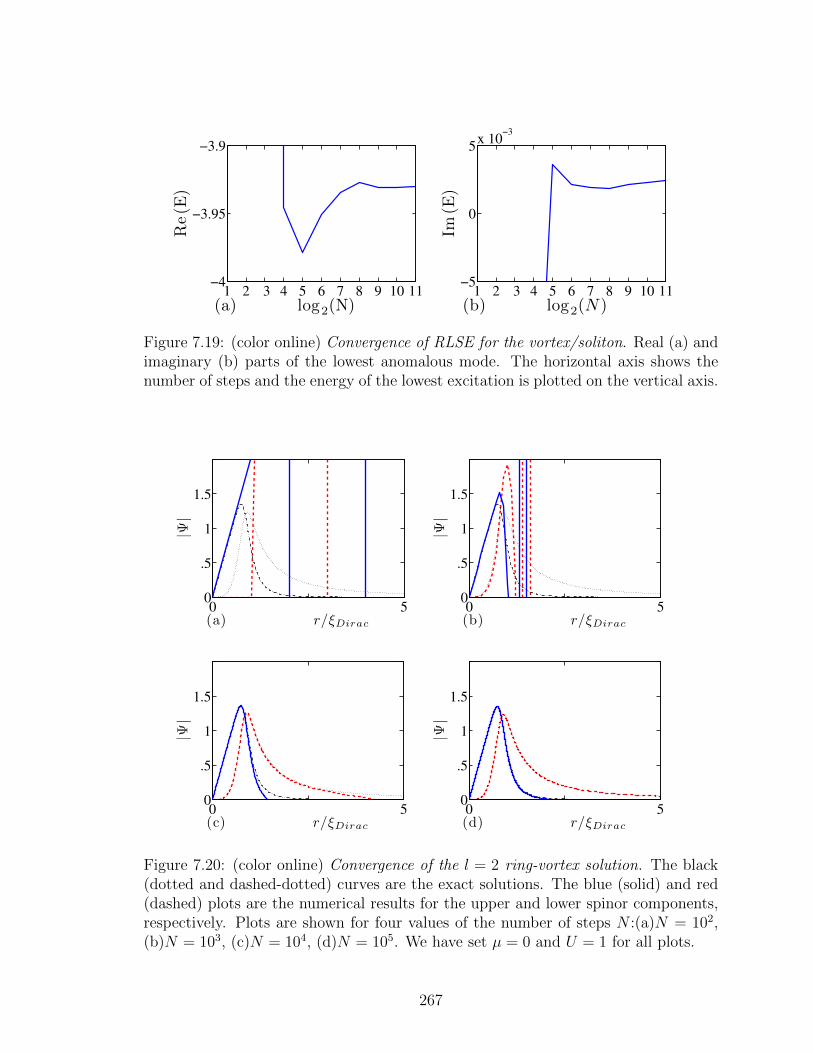
1 2 3 4 5 6 7 8 9 10 11−4

−3.95

−3.9

(a) log2(N)

Re(E

)

1 2 3 4 5 6 7 8 9 10 11−5

0

5x 10

−3

(b) log2(N )

Im(E

)

Figure 7.19: (color online) Convergence of RLSE for the vortex/soliton. Real (a) andimaginary (b) parts of the lowest anomalous mode. The horizontal axis shows thenumber of steps and the energy of the lowest excitation is plotted on the vertical axis.

0 50

.5

1

1.5

(a) r/ξDirac

|Ψ|

0 50

.5

1

1.5

(b) r/ξDirac

|Ψ|

0 50

.5

1

1.5

(c) r/ξDirac

|Ψ|

0 50

.5

1

1.5

(d) r/ξDirac

|Ψ|

Figure 7.20: (color online) Convergence of the l = 2 ring-vortex solution. The black(dotted and dashed-dotted) curves are the exact solutions. The blue (solid) and red(dashed) plots are the numerical results for the upper and lower spinor components,respectively. Plots are shown for four values of the number of steps N :(a)N = 102,(b)N = 103, (c)N = 104, (d)N = 105. We have set µ = 0 and U = 1 for all plots.

267

CHAPTER 8

THE NONLINEAR DIRAC EQUATION: RELATIVISTIC SOLITONS AND

MASS GAPS

L. H. Haddad, C. M. Weaver, and Lincoln D. Carr, Physical Review A,

under review, 2012.

Abstract

We present a thorough analysis of solitons which solve the one-dimensional (1D)

zigzag and armchair nonlinear Dirac equation (NLDE) for a Bose-Einstein condensate

(BEC) in a honeycomb lattice, where the two types of NLDEs correspond to the two

independent directions in analogy to the narrowest of graphene nanoribbons. Analyt-

ical as well as numerical soliton two-component spinor solutions are obtained. These

include analytical spatially infinite arrays of bright two-spinor solitons. In addition,

we find a gray line-soliton and compute its discrete spectra for several spatially quan-

tized states in a harmonic potential. The strong region of the harmonic trap provides

a unique opportunity to study the BEC analog of Klein-tunneling. By solving the

relativistic linear stability equations (RLSE) for a BEC of 87Rb atoms, we find that

most of our solutions are either stable or unstable on times scales longer than the

lifetime of experiments. Nambu-Goldstone modes are detected in the linear spectra

for all of our solutions. We study the effect of various types of mass gaps on the

solution space of the NLDE. In particular, the gap produced by a modulation of the

nearest-neighbor hopping allows for a general mapping of our embedded solitons into

269

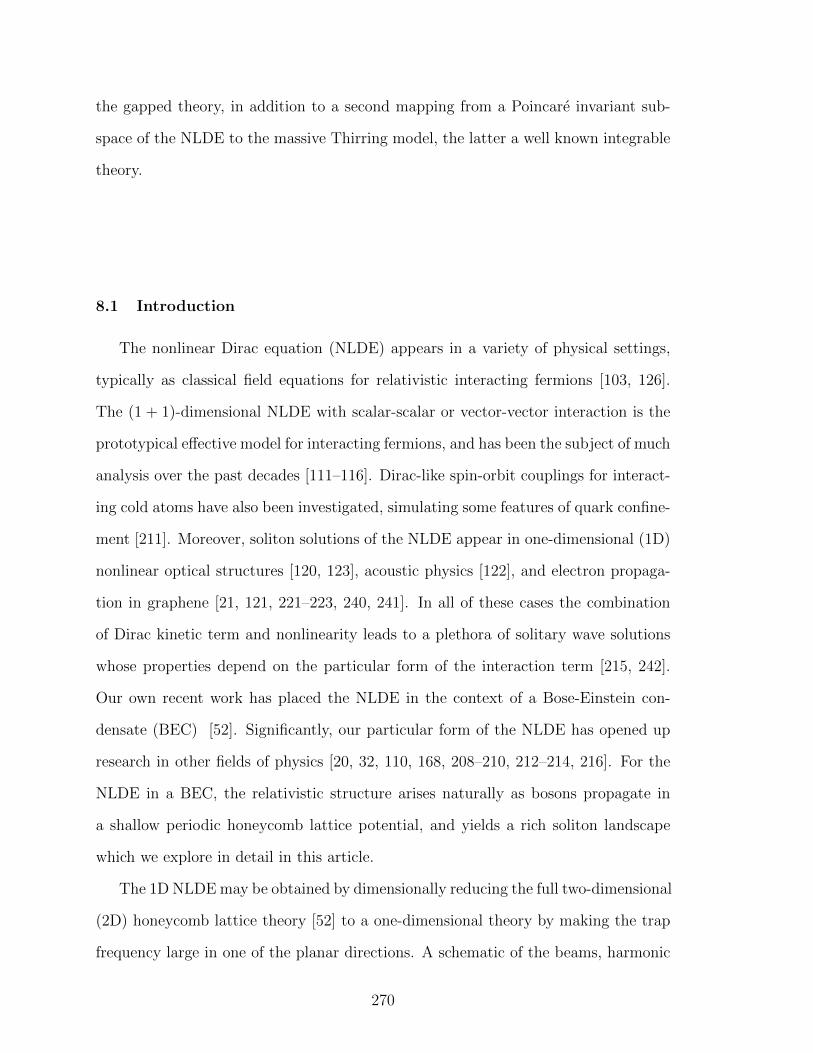
the gapped theory, in addition to a second mapping from a Poincare invariant sub-

space of the NLDE to the massive Thirring model, the latter a well known integrable

theory.

8.1 Introduction

The nonlinear Dirac equation (NLDE) appears in a variety of physical settings,

typically as classical field equations for relativistic interacting fermions [103, 126].

The (1 + 1)-dimensional NLDE with scalar-scalar or vector-vector interaction is the

prototypical effective model for interacting fermions, and has been the subject of much

analysis over the past decades [111–116]. Dirac-like spin-orbit couplings for interact-

ing cold atoms have also been investigated, simulating some features of quark confine-

ment [211]. Moreover, soliton solutions of the NLDE appear in one-dimensional (1D)

nonlinear optical structures [120, 123], acoustic physics [122], and electron propaga-

tion in graphene [21, 121, 221–223, 240, 241]. In all of these cases the combination

of Dirac kinetic term and nonlinearity leads to a plethora of solitary wave solutions

whose properties depend on the particular form of the interaction term [215, 242].

Our own recent work has placed the NLDE in the context of a Bose-Einstein con-

densate (BEC) [52]. Significantly, our particular form of the NLDE has opened up

research in other fields of physics [20, 32, 110, 168, 208–210, 212–214, 216]. For the

NLDE in a BEC, the relativistic structure arises naturally as bosons propagate in

a shallow periodic honeycomb lattice potential, and yields a rich soliton landscape

which we explore in detail in this article.

The 1D NLDE may be obtained by dimensionally reducing the full two-dimensional

(2D) honeycomb lattice theory [52] to a one-dimensional theory by making the trap

frequency large in one of the planar directions. A schematic of the beams, harmonic

270

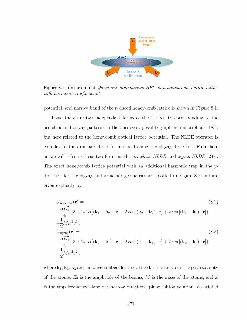
Honeycomb

optical lattice

lasers

BEC

Harmonic

confinement k1 k2

k3

Figure 8.1: (color online) Quasi-one-dimensional BEC in a honeycomb optical latticewith harmonic confinement.

potential, and narrow band of the reduced honeycomb lattice is shown in Figure 8.1.

Thus, there are two independent forms of the 1D NLDE corresponding to the

armchair and zigzag patterns in the narrowest possible graphene nanoribbons [183],

but here related to the honeycomb optical lattice potential. The NLDE operator is

complex in the armchair direction and real along the zigzag direction. From here

on we will refer to these two forms as the armchair NLDE and zigzag NLDE [243].

The exact honeycomb lattice potential with an additional harmonic trap in the y-

direction for the zigzag and armchair geometries are plotted in Figure 8.2 and are

given explicitly by

Uarmchair(r) = (8.1)

−αE20

4(3 + 2 cos [(k1 − k2) · r] + 2 cos [(k2 − k3) · r] + 2 cos [(k1 − k3) · r])

+1

2Mω2y2 ,

Uzigzag(r) = (8.2)

−αE20

4(3 + 2 cos [(k2 − k1) · r] + 2 cos [(k1 − k3) · r] + 2 cos [(k2 − k3) · r])

+1

2Mω2y2 ,

where k1, k2, k3 are the wavenumbers for the lattice laser beams, α is the polarizability

of the atoms, E0 is the amplitude of the beams, M is the mass of the atoms, and ω

is the trap frequency along the narrow direction. pinor soliton solutions associated

271

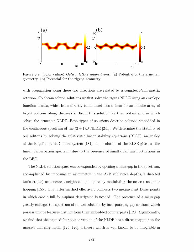
y

x

y

x

(a) (b)

Figure 8.2: (color online) Optical lattice nanoribbons. (a) Potential of the armchairgeometry. (b) Potential for the zigzag geometry.

with propagation along these two directions are related by a complex Pauli matrix

rotation. To obtain soliton solutions we first solve the zigzag NLDE using an envelope

function ansatz, which leads directly to an exact closed form for an infinite array of

bright solitons along the x-axis. From this solution we then obtain a form which

solves the armchair NLDE. Both types of solutions describe solitons embedded in

the continuous spectrum of the (2 + 1)D NLDE [244]. We determine the stability of

our solitons by solving the relativistic linear stability equations (RLSE), an analog

of the Bogoliubov de-Gennes system [184]. The solution of the RLSE gives us the

linear perturbation spectrum due to the presence of small quantum fluctuations in

the BEC.

The NLDE solution space can be expanded by opening a mass gap in the spectrum,

accomplished by imposing an asymmetry in the A/B sublattice depths, a directed

(anisotropic) next-nearest neighbor hopping, or by modulating the nearest neighbor

hopping [155]. The latter method effectively connects two inequivalent Dirac points

in which case a full four-spinor description is needed. The presence of a mass gap

greatly enlarges the spectrum of soliton solutions by incorporating gap solitons, which

possess unique features distinct from their embedded counterparts [120]. Significantly,

we find that the gapped four-spinor version of the NLDE has a direct mapping to the

massive Thirring model [125, 126], a theory which is well known to be integrable in

272

both the quantum and classical sense. At the level of the wavefunction, the real and

imaginary parts of the NLDE spinor components are mapped to the upper and lower

spinor components in the Thirring model, respectively. The Thirring spinors possess

exact relativistic invariance and so are comprised of equal admixtures of positive

and negative energy solutions in the NLDE picture. The fact that our mapping

works for a subspace of NLDE solutions suggests integrability but is certainly not

conclusive. A complete analysis of the problem would require constructing a Lax

pair representation of the NLDE, in addition to using other formal methods such

as general Painleve analysis, singular manifold methods, or Darboux and Backlund

transformations [103, 245–250]. For the latter test, the key question to address is

whether or not our mapping to the Thirring model can be classified as an auto-

Backlund or hetero-Backlund transformation.

8.2 Soliton Solutions of the NLDE

In this section we solve the NLDE without a mass gap. The parameters which

enter directly into the NLDE and will therefore appear in all of our solutions, are the

effective speed of light cl = tha√

3/2~ and the particle interaction U = Lzgn23√

3a2/8,

where U is the 2D optical lattice renormalized version of the usual interaction g =

4π~2as/M . Appearing in these definitions are the average particle density n = N/V ,

the s-wave scattering length as, the vertical oscillator length Lz, the mass M of

the constituent atoms in the BEC, the lattice constant a, and the hopping en-

ergy th. For the hopping energy, we use a semiclassical estimate given by th ≡

1.861 (V0/ER)3/4ER exp(−1.582

√V0/ER

)[77]. A complete discussion of NLDE pa-

rameters and constraints can be found in [cite our NP paper on the axiv]

The NLDE for two inequivalent Dirac points describes the dynamics of a Dirac

four-spinor of the form Ψ ≡ (Ψ+, Ψ−)T , with the upper (+) and lower (−) two-spinors

relating to opposite K and K′ points of the honeycomb lattice. The full NLDE in

this case is

273

i~γµ∂µΨ− U4∑i=1

(MiΨ)(Ψ†Mi) Ψ = 0 . (8.3)

The matrices γµ are the usual Dirac matrices and the interaction terms are encapsu-

lated in the summation with the matrices Mi constructed to give the correct cubic

nonlinearites, local to each spinor component [52]. The interactions do not couple dif-

ferent spinor components so we focus on the equations for a two-spinor in rectangular

coordinates

i~ ∂tψA = −i~cl (∂x − i∂y)ψB + U |ψA|2 ψA (8.4)

i~ ∂tψB = −i~cl (∂x + i∂y)ψA + U |ψB|2 ψB , (8.5)

with the full solution expressed as a linear combination of solutions from each Dirac

point. Note the presence of the effective speed of light, cl, and interaction strength,

U . Eqs. (8.4)-(8.5) allow for one-dimensional (1D) solutions by taking ψA and ψB to

vary in only one direction while remaining constant in the other. We are interested

in stationary states so we take the time-dependence to be the usual exponential

factor with the chemical potential as the frequency. We then write: ψA(x, t) =

exp(−iµt/~)fA(x) and ψB(x, t) = exp(−iµt/~)fB(x), where fA(x) and fB(x) are

taken to be functions of the single variable x and µ is the usual chemical potential.

Note that choosing the y-direction adjusts the relative phase between the spinor

components. Eqs. (8.4)-(8.5) become

µfA(x) = −i~cl ∂xfB(x) + U |fA(x)|2fA(x) (8.6)

µfB(x) = −i~cl ∂xfA(x) + U |fB(x)|2fB(x) . (8.7)

This is the time-independent 1D NLDE for the armchair direction of the honeycomb

lattice. Notice that taking fA → ifA we converts the real zigzag version corresponding

to the y-direction. It is natural to retain the x notation when discussing either form

274

of the NLDE, thus we write the zigzag version as

µfA(x) = −~cl ∂xfB(x) + U |fA(x)|2fA(x) (8.8)

µfB(x) = ~cl ∂xfA(x) + U |fB(x)|2fB(x) . (8.9)

8.3 Bright Soliton Train

An exact real solution of the NLDE may be obtained using the form

Ψ(x) = η(x)

(cosϕ(x)

sinϕ(x)

), (8.10)

where we have assumed only that the wavefunction is real. Substituting Eq. (8.10)

into Eqs. (8.8)-(8.9), multiplying by cosϕ and sinϕ, respectively, then adding the

resulting equations gives

dϕ

dx= − µ

~cl[1− η2 (U/µ)(cos4ϕ+ sin4ϕ)

](8.11)

To obtain a second equation we multiply Eqs. (8.8)-(8.9) by cosϕ and sinϕ, respec-

tively, then subtract the resulting equations which yields

d(lnη)

dx=

U

4~clη2 sin(4ϕ) . (8.12)

Note that we have divided through by η to arrive at Eqs. (8.11)-(8.12). Equa-

tions (8.11)-(8.12) can be combined by back substitution to get

[sin(4ϕ)

cos4ϕ+ sin4ϕ

](ϕ+

µx

~cl

)′= 4 (lnη)′ (8.13)

where the prime notation indicates differentiation with respect to x. From Eq. (8.13),

we may obtain a formal expression for η:

η4 = exp

[∫dx

sin(4ϕ)

cos4ϕ+ sin4ϕ

(ϕ+

µx

~cl

)′]. (8.14)

275

To solve Eq. (8.14), we choose the linear form ϕ(x) = κx, obtain an explicit form

for η(x) which we then substitute into Eq. (8.11) to determine the constant κ and

obtain a relation for the chemical potential µ and the interaction U . Equation (8.14)

becomes

η4 = exp

[(κ+ µ/~cl)

∫dx

sin(4κx)

cos4κx+ sin4κx

]. (8.15)

Integrating gives

η(x) =(cos4κx+ sin4κx

)−(1+µ/κ~cl)/4 . (8.16)

Substituting this result into Eq. (8.11) and using the linear ansatz, gives the expres-

sion

κ = − µ

~cl

[1− U

µ

(cos4κx+ sin4κx

)1−(1+µ/κ~cl)/2]. (8.17)

In order for this expression to be true, it must be that the exponent of the spatial

functions is identically zero. Equation (8.17) then gives the two conditions

1

2− µ

2κ~cl= 0 , (8.18)

− µ

~cl

(1− U

µ

)= κ , (8.19)

which may be solved to give

κ =µ

~cl, (8.20)

µ = 2U . (8.21)

The corresponding solution is then

Ψzigzag(x) =(cos4κx+ sin4κx

)−1/2

(cosκx

sinκx

), (8.22)

276

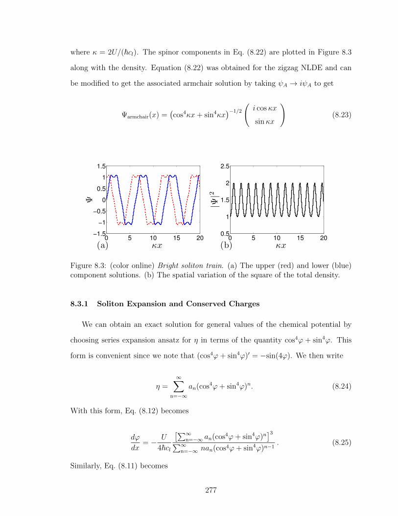
where κ = 2U/(~cl). The spinor components in Eq. (8.22) are plotted in Figure 8.3

along with the density. Equation (8.22) was obtained for the zigzag NLDE and can

be modified to get the associated armchair solution by taking ψA → iψA to get

Ψarmchair(x) =(cos4κx+ sin4κx

)−1/2

(i cosκx

sinκx

)(8.23)

0 5 10 15 20−1.5

−1

−0.5

0

0.5

1

1.5

(a) κx

Ψ

0 5 10 15 200.5

1

1.5

2

2.5

(b) κx

|Ψ|2

Figure 8.3: (color online) Bright soliton train. (a) The upper (red) and lower (blue)component solutions. (b) The spatial variation of the square of the total density.

8.3.1 Soliton Expansion and Conserved Charges

We can obtain an exact solution for general values of the chemical potential by

choosing series expansion ansatz for η in terms of the quantity cos4ϕ + sin4ϕ. This

form is convenient since we note that (cos4ϕ+ sin4ϕ)′ = −sin(4ϕ). We then write

η =∞∑

n=−∞

an(cos4ϕ+ sin4ϕ)n. (8.24)

With this form, Eq. (8.12) becomes

dϕ

dx= − U

4~cl

[∑∞n=−∞ an(cos4ϕ+ sin4ϕ)n

]3∑∞n=−∞ nan(cos4ϕ+ sin4ϕ)n−1

. (8.25)

Similarly, Eq. (8.11) becomes

277

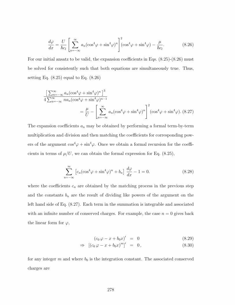
dϕ

dx=

U

~cl

[∞∑

n=−∞

an(cos4ϕ+ sin4ϕ)n

]2

(cos4ϕ+ sin4ϕ)− µ

~cl. (8.26)

For our initial ansatz to be valid, the expansion coefficients in Eqs. (8.25)-(8.26) must

be solved for consistently such that both equations are simultaneously true. Thus,

setting Eq. (8.25) equal to Eq. (8.26)

[∑∞n=−∞ an(cos4ϕ+ sin4ϕ)n

]34∑∞

n=−∞ nan(cos4ϕ+ sin4ϕ)n−1

=µ

U−[∞∑

n=−∞

an(cos4ϕ+ sin4ϕ)n

]2

(cos4ϕ+ sin4ϕ). (8.27)

The expansion coefficients an may be obtained by performing a formal term-by-term

multiplication and division and then matching the coefficients for corresponding pow-

ers of the argument cos4ϕ + sin4ϕ. Once we obtain a formal recursion for the coeffi-

cients in terms of µ/U , we can obtain the formal expression for Eq. (8.25),

∞∑n=−∞

[cn(cos4ϕ+ sin4ϕ)n + bn

] dϕdx− 1 = 0. (8.28)

where the coefficients cn are obtained by the matching process in the previous step

and the constants bn are the result of dividing like powers of the argument on the

left hand side of Eq. (8.27). Each term in the summation is integrable and associated

with an infinite number of conserved charges. For example, the case n = 0 gives back

the linear form for ϕ,

(c0 ϕ− x+ b0x)′ = 0 (8.29)

⇒ [(c0 ϕ− x+ b0x)m]′

= 0 , (8.30)

for any integer m and where b0 is the integration constant. The associated conserved

charges are

278

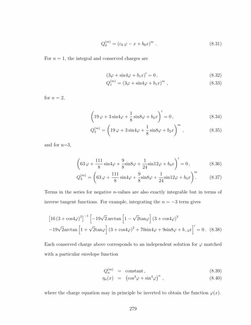
Q(m)0 = (c0 ϕ− x+ b0x)m . (8.31)

For n = 1, the integral and conserved charges are

(3ϕ+ sin4ϕ+ b1x)′ = 0 , (8.32)

Q(m)1 = (3ϕ+ sin4ϕ+ b1x)m , (8.33)

for n = 2,

(19ϕ+ 3 sin4ϕ+

1

8sin8ϕ+ b2x

)′= 0 , (8.34)

Q(m)2 =

(19ϕ+ 3 sin4ϕ+

1

8sin8ϕ+ b2x

)m, (8.35)

and for n=3,

(63ϕ+

111

8sin4ϕ+

9

8sin8ϕ+

1

24sin12ϕ+ b3x

)′= 0 , (8.36)

Q(m)3 =

(63ϕ+

111

8sin4ϕ+

9

8sin8ϕ+

1

24sin12ϕ+ b3x

)m. (8.37)

Terms in the series for negative n-values are also exactly integrable but in terms of

inverse tangent functions. For example, integrating the n = −3 term gives

[16 (3 + cos4ϕ)2]−1

[−19√

2 arctan[1−√

2tanϕ]

(3 + cos4ϕ)2

−19√

2arctan[1 +√

2tanϕ]

(3 + cos4ϕ)2 + 70sin4ϕ+ 9sin8ϕ+ b−3x]′

= 0 . (8.38)

Each conserved charge above corresponds to an independent solution for ϕ matched

with a particular envelope function

Q(m)n = constant , (8.39)

ηn(x) =(cos4ϕ+ sin4ϕ

)n, (8.40)

where the charge equation may in principle be inverted to obtain the function ϕ(x).

279

There is a definite relationship between this formal series approach and the slowly

varying approximate solutions we obtained previously. We point out the fact that

3 + cos4x = (cos4x + sin4x)/4, so that apart from a factor of 4, our earlier solu-

tions correspond to the linear approximation for ϕ in Eq. (8.28) for each term in

Eq. (8.24) but with real, continuous valued exponents. The negative exponent terms

in Eq. (8.24) map to solutions of the type shown in ??, while positive exponent terms

map to those in ??. Thus, our series expansion in principle contains all solitons of

the 1D NLDE, with the higher order terms in Eq. (8.28) representing higher soliton

resonances.

8.3.2 Numerical Solitons

The profile for a topological soliton (µ 6= 0) can be obtained using a numerical

shooting method [230]. The most direct approach is to express Eqs. (8.8)-(8.9) in

terms of the dimensionless spatial variable χ ≡ (U/~cl)x. The functions fA(χ) and

fB(χ) are then expanded in power series around χ = 0

fA(χ) =∞∑j=0

ajχj , fB(χ) =

∞∑j=0

bjχj , (8.41)

where the aj and bj are the expansion coefficients. Since we are solving two coupled

first order equations, we require the initial conditions fA(0) and fB(0). Substituting

into Eqs. (8.8)-(8.9) gives us the behavior of the solution at the origin:

f ′A(0) ∼ 1

~cl[µ− UfB(0)2

]fB(0) (8.42)

f ′B(0) ∼ − 1

~cl[µ− UfA(0)2

]fA(0). (8.43)

The form of the 1D NLDE shows that for any index j ≥ 0, a2j+1 and b2j are related

through a recursion formula, likewise a2j and b2j+1 are also related. To obtain a

soliton solutions using the shooting method, we first fix either a0 or b0 then vary the

280

other until we obtain convergence to a the desired precision. Although it seems that

both a0 and b0 are free parameters, fixing one to a different value before shooting

results in a spatially translated final solution. We take b0 = 0 and solve for the value

a0 = asoliton0 which gives the desired form. Figure 8.4(c) shows our numerical shooting

results for the line soliton. This is obtained for

asoliton0 = 0.94640402384. (8.44)

In Figure 8.4(a) and (b) we show the solution for values of a0 > asoliton0 . At larger

values of a0, the interaction energy becomes more pronounced and we start to pick

up some of the excited soliton states which can be seen in Figure 8.4(a) and (b). For

values a0 < asoliton0 , the effect of the interaction is reduced, Figure 8.4(d) and (e), until

finally we see the free particle sine and cosine forms appearing in Figure 8.4(f).

The solution in Figure 8.4(c) is an example of a gray soliton since the density

of atoms is constant everywhere except near the line where the A and B sublattice

amplitudes meet. A comparison of the gray soliton and bright soliton densities is

shown in Figure 8.5. We can see that the line soliton is at the boundary between two

regimes: the strongly interacting bright soliton regime shown in Figure 8.4(a), and

the weakly interacting free-particle regime in Figure 8.4(f).

8.4 Mass Gaps for the NLDE

The introduction of a mass gap into our system greatly expands its versatil-

ity, allowing for a richer structures in the nonlinear landscape. Masses in general

graphene-like systems with fermions have been studied extensively [155], and provide

a foundation for our analysis of mass gaps within the analog bosonic system. In this

section we define and then discuss the various key types of gaps possible for bosons in

the honeycomb optical lattice, then present the particular features of solitons in the

presence of a gap and discuss how they relate back to our gapless solitons. We provide

281

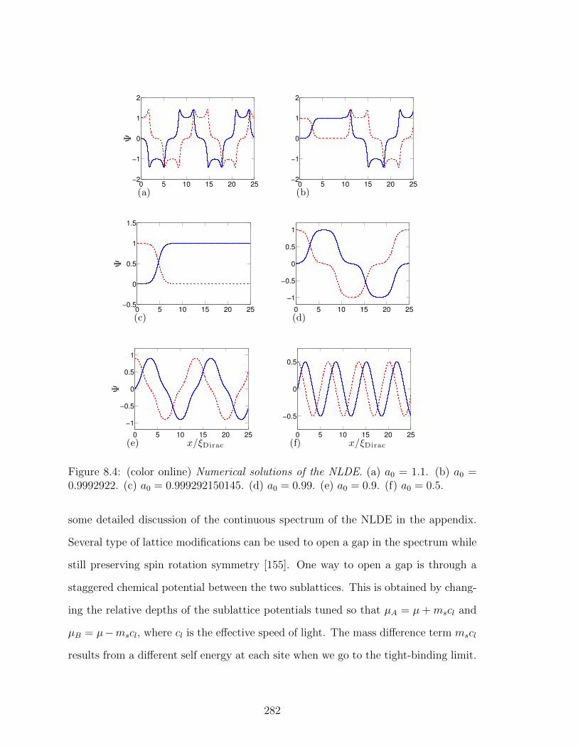
0 5 10 15 20 25−2

−1

0

1

2

(a)

Ψ

0 5 10 15 20 25−2

−1

0

1

2

(b)

0 5 10 15 20 25−0.5

0

0.5

1

1.5

(c)

Ψ

0 5 10 15 20 25

−1

−0.5

0

0.5

1

(d)

0 5 10 15 20 25

−1

−0.5

0

0.5

1

(e) x/ξDirac

Ψ

0 5 10 15 20 25

−0.5

0

0.5

(f) x/ξDirac

Figure 8.4: (color online) Numerical solutions of the NLDE. (a) a0 = 1.1. (b) a0 =0.9992922. (c) a0 = 0.999292150145. (d) a0 = 0.99. (e) a0 = 0.9. (f) a0 = 0.5.

some detailed discussion of the continuous spectrum of the NLDE in the appendix.

Several type of lattice modifications can be used to open a gap in the spectrum while

still preserving spin rotation symmetry [155]. One way to open a gap is through a

staggered chemical potential between the two sublattices. This is obtained by chang-

ing the relative depths of the sublattice potentials tuned so that µA = µ + mscl and

µB = µ−mscl, where cl is the effective speed of light. The mass difference term mscl

results from a different self energy at each site when we go to the tight-binding limit.

282

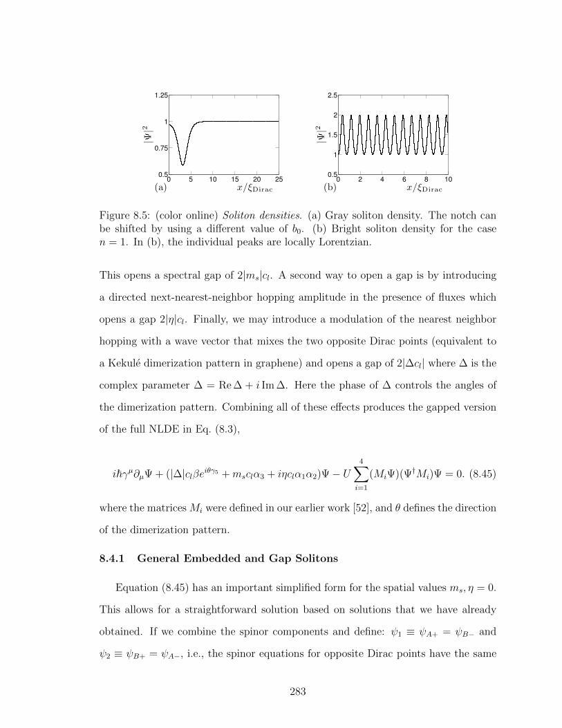
0 5 10 15 20 250.5

0.75

1

1.25

(a) x/ξDirac

|Ψ|2

0 2 4 6 8 100.5

1

1.5

2

2.5

(b) x/ξDirac

|Ψ|2

Figure 8.5: (color online) Soliton densities. (a) Gray soliton density. The notch canbe shifted by using a different value of b0. (b) Bright soliton density for the casen = 1. In (b), the individual peaks are locally Lorentzian.

This opens a spectral gap of 2|ms|cl. A second way to open a gap is by introducing

a directed next-nearest-neighbor hopping amplitude in the presence of fluxes which

opens a gap 2|η|cl. Finally, we may introduce a modulation of the nearest neighbor

hopping with a wave vector that mixes the two opposite Dirac points (equivalent to

a Kekule dimerization pattern in graphene) and opens a gap of 2|∆cl| where ∆ is the

complex parameter ∆ = Re ∆ + i Im ∆. Here the phase of ∆ controls the angles of

the dimerization pattern. Combining all of these effects produces the gapped version

of the full NLDE in Eq. (8.3),

i~γµ∂µΨ + (|∆|clβeiθγ5 +msclα3 + iηclα1α2)Ψ− U4∑i=1

(MiΨ)(Ψ†Mi)Ψ = 0. (8.45)

where the matrices Mi were defined in our earlier work [52], and θ defines the direction

of the dimerization pattern.

8.4.1 General Embedded and Gap Solitons

Equation (8.45) has an important simplified form for the spatial values ms, η = 0.

This allows for a straightforward solution based on solutions that we have already

obtained. If we combine the spinor components and define: ψ1 ≡ ψA+ = ψB− and

ψ2 ≡ ψB+ = ψA−, i.e., the spinor equations for opposite Dirac points have the same

283

form, and we find that ψ1 and ψ2 satisfy the equations

i~ ∂t(ψ1

ψ2

)=

(U |ψ1|2 + |∆|clcosθ −i~clD∗

−i~clD U |ψ2|2 + |∆|clcosθ

)(ψ1

ψ2

), (8.46)

which, for stationary solutions with chemical potential µg (redefined for the gapped

case), reduce to the time-independent NLDE with mass gap:

−i~clD∗ψ2 + U |ψ1|2 ψ1 = (µg + |∆|clcosθ)ψ1

−i~clD∗ψ1 + U |ψ1|2 ψ2 = (µg + |∆|clcosθ)ψ2 , (8.47)

where subscripted µg indicates the chemical potential in the gapped theory. Eq. (8.47)

is exactly the two-spinor NLDE modified by the gap |∆|cosθ along with the identi-

fications ψ1 ≡ ψA, ψ2 = ψB. This means that all of our previous solutions are valid

here, and we can read off the chemical potential µ for the gapless theory with the

identification µg = µ− |∆|clcosθ for the gaped theory. The characteristic features of

the different types of gapped solutions are as follows:

1. For the special case where θ = nπ, solutions with non-zero µ in the gapless

theory map to solitons that are either inside the gap or are embedded in the

continuous spectrum, depending on the phase integer n. For example, a soliton

solution with chemical potential µ = 2U maps to µg = 2U ± |∆|cl. The positive

sign sets the soliton inside the gap when |µg| < |∆|cl, which is satisfied if |∆|cl >

U > |∆|cl/2, for positive µg. The negative sign embeds the soliton within the

continuous spectrum. In this case the chemical potential µg = 2U+|∆|cl. Thus,

the chemical potential of the gapless solution is shifted up by |∆|cl.

2. For zero-chemical potential solutions, we find the condition µg = ±|∆|cl (for

θ = nπ). These correspond to solitons whose components both vanish for

x→∞. Again, these solutions have their chemical potentials shifted by |∆|cl,

reside at the lower (negative sign) and upper (positive sign) edges of the gap.

284

3. By tuning the gap phase angle θ, we can continuously adjust the chemical

potential µg setting it inside or outside the gap.

4. It is important to note that for the general case where ms, η 6= 0, exact solutions

are still likely to be found but further analysis is required, since we cannot use

the same mapping as we have done here.

8.4.2 Mapping to the Integrable Thirring Model

As discussed in the last section, the mass gaps mscl, ηcl, and |∆|cle±iθ are for in-

equivalent lattice depths, next-nearest-neighbor hopping, and modulation of nearest-

neighbor hopping, respectively. Takingms = η = 0 and restricting to the x−direction,

the NLDE for finite-energy stationary solutions can be written compactly as

(µ 1− D) Ψ = 0 , (8.48)

where 1 is the 4× 4 unit matrix and D is defined as

D ≡

U |ψA+|2 −i~cl ddx |∆|eiθ 0

−i~cl ddx U |ψB+|2 0 |∆|eiθ|∆|e−iθ 0 U |ψB−|2 i~cl ddx

0 |∆|e−iθ i~cl ddx U |ψA−|2

, (8.49)

8.4.3 Derivation of the Mapping

Equation (8.49) has a symmetry which allows for a consistent solution of the form

ψA+ = ψB+ ≡ ψ , ψA− = ψB− ≡ ψ∗ . (8.50)

Substituting this ansatz into Eq. (8.49) transforms the lower two equations into the

conjugates of the upper two. The four-spinor wavefunction in Eq. (8.48) becomes

Ψ = (ψ, ψ, ψ∗, ψ∗)T , and D becomes

285

D =

U |ψ|2 −i ~cl ddx |∆|eiθ 0

−i ~cl ddx U |ψ|2 0 |∆|eiθ|∆|e−iθ 0 U |ψ|2 i ~cl ddx

0 |∆|e−iθ i ~cl ddx U |ψ|2

. (8.51)

By inspection we see that Eq. (8.51) is equivalent to the single equation

µψ = −i ~cld

dxψ + |∆|cleiθψ∗ + U |ψ|2ψ . (8.52)

Next, we show that the real and imaginary parts of Eq. (8.52) satisfy the classical

field equations for the massive Thirring model [126]. Splitting ψ(x) into real and

imaginary parts: ψ(x) = u(x) + iv(x), and taking the modulation angle θ = π,

Eq. (8.52) becomes

µ(u+ iv) = −i~cld

dx(u+ iv) + |∆|cl(u− iv) + U(u2 + v2)(u+ iv). (8.53)

Finally, equating real and imaginary parts on both sides yields equations for u and

v:

µu = ~cld

dxv − |∆|clu+ U(u2 + v2)u (8.54)

µv = −~cld

dxu+ |∆|clv + U(u2 + v2)v . (8.55)

If we consider negative energy solutions of the NLDE so that µ = −|µ|, and also take

v → −v, we obtain

~cldu

dx+ (|∆|cl + |µ|)v + U(u2 + v2)v = 0 (8.56)

~cldv

dx+ (|∆|cl − |µ|)u− U(u2 − v2)u = 0 . (8.57)

With the definitions: m ≡ |∆|/~, E ≡ |µ|/~cl, g2 ≡ U/~cl, we obtain

286

du

dx+ (m+ E)v + g2(u2 + v2)v = 0 (8.58)

dv

dx+ (m− E)u− g2(u2 + v2)u = 0 . (8.59)

This is the massive Thirring model for interacting fermions with vector-vector interac-

tion. We note that Eqs. (8.58)-(8.59) form an integrable system: see for example [126]

for early work; [96] for connection to nonlinear optics; and [103] for a generalization

to arbitrary powers of the interaction. Note that the massless Thirring model is

obtained by setting the gap parameter |∆| to zero.

8.4.4 NLDE Gap Solitons from the Thirring Mapping

Equations (8.58)-(8.59) can be derived by minimizing the action for fermions with

vector-vector interaction written in the usual compact form found in the literature

L = Ψ(iγµ∂µ −m)Ψ +g2

2

(ΨγµΨ

)2, (8.60)

where, here one must recall that in 1D the γµ matrices are the usual Pauli matrices and

we have omitted factors of the speed of light c to be consistent with the literature.

It is important to emphasize that the interaction term here is a Lorentz invariant

quantity in contrast to its NLDE counterpart. Soliton solutions can be found using

the parameterization

ψ(x) ≡(u(x)

v(x)

)= R(x)

(cosφ(x)

sinφ(x)

). (8.61)

A first integral of Eqs. (8.58)-(8.59) can be obtained using conservation of the energy-

momentum tensor [103], to arrive at

φ(x) = tan−1(α tanh βx) , (8.62)

287

where

α =

√m− Em+ E

, β =√m2 − E2 , (8.63)

and

R(x) =

√2 β sech βx

g√

(m+ E)(1 + α2 tanh2 βx). (8.64)

It is significant that these solutions are stable for 0 < E < m, i.e., when the energy

is inside the gap, consequently such solutions are usually referred to as gap solitons.

Having obtained our solution, we now map it back to the NLDE four-spinor compo-

nents to arrive at

ψA+(x) =

√2~cl αβ/U sech βx

(1 + α2 tanh2 βx)(1− i α tanh βx) , (8.65)

ψB+(x) =

√2~cl αβ/U sech βx

(1 + α2 tanh2 βx)(1− i α tanh βx) , (8.66)

ψB−(x) =

√2~cl αβ/U sech βx

(1 + α2 tanh2 βx)(1 + i α tanh βx) , (8.67)

ψA−(x) =

√2~cl αβ/U sech βx

(1 + α2 tanh2 βx)(1 + i α tanh βx) , (8.68)

with the parameters mapped to the NLDE parameters by

α =

√|∆| − |µ||∆|+ |µ| , β =

√∆2 − µ2 . (8.69)

The real and imaginary parts of these solutions are plotted in Figure 8.6 for several

values of the parameters α, β, and U .

288

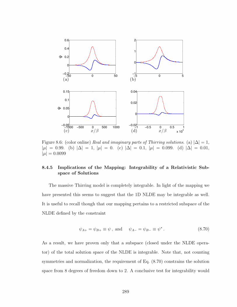
−50 0 50−0.2

0

0.2

0.4

0.6

(a)

Ψ

−5 0 5−1

0

1

2

(b)

−1000 −500 0 500 1000−0.05

0

0.05

0.1

0.15

(c) x/β

Ψ

−1 −0.5 0 0.5 1

x 104

−0.02

0

0.02

0.04

(d) x/β

Figure 8.6: (color online) Real and imaginary parts of Thirring solutions. (a) |∆| = 1,|µ| = 0.99. (b) |∆| = 1, |µ| = 0. (c) |∆| = 0.1, |µ| = 0.099. (d) |∆| = 0.01,|µ| = 0.0099

8.4.5 Implications of the Mapping: Integrability of a Relativistic Sub-space of Solutions

The massive Thirring model is completely integrable. In light of the mapping we

have presented this seems to suggest that the 1D NLDE may be integrable as well.

It is useful to recall though that our mapping pertains to a restricted subspace of the

NLDE defined by the constraint

ψA+ = ψB+ ≡ ψ , and ψA− = ψB− ≡ ψ∗ . (8.70)

As a result, we have proven only that a subspace (closed under the NLDE opera-

tor) of the total solution space of the NLDE is integrable. Note that, not counting

symmetries and normalization, the requirement of Eq. (8.70) constrains the solution

space from 8 degrees of freedom down to 2. A conclusive test for integrability would

289

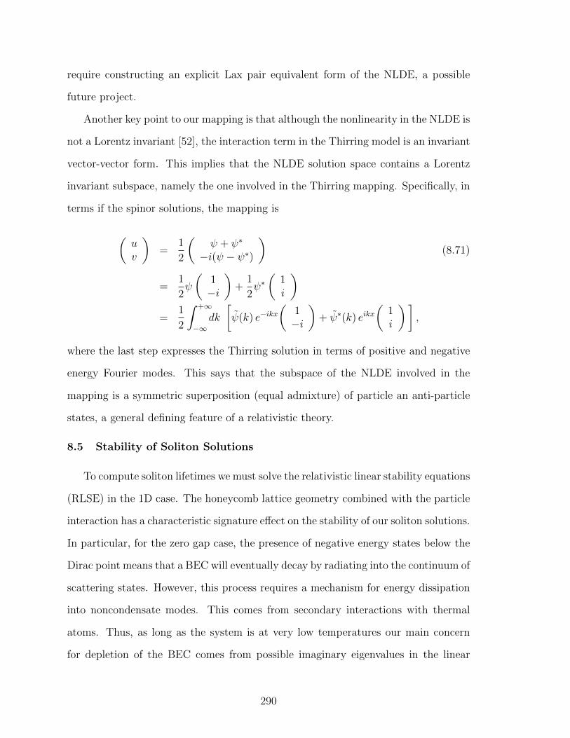
require constructing an explicit Lax pair equivalent form of the NLDE, a possible

future project.

Another key point to our mapping is that although the nonlinearity in the NLDE is

not a Lorentz invariant [52], the interaction term in the Thirring model is an invariant

vector-vector form. This implies that the NLDE solution space contains a Lorentz

invariant subspace, namely the one involved in the Thirring mapping. Specifically, in

terms if the spinor solutions, the mapping is

(uv

)=

1

2

(ψ + ψ∗

−i(ψ − ψ∗)

)(8.71)

=1

2ψ

(1−i

)+

1

2ψ∗(

1i

)=

1

2

∫ +∞

−∞dk

[ψ(k) e−ikx

(1−i

)+ ψ∗(k) eikx

(1i

)],

where the last step expresses the Thirring solution in terms of positive and negative

energy Fourier modes. This says that the subspace of the NLDE involved in the

mapping is a symmetric superposition (equal admixture) of particle an anti-particle

states, a general defining feature of a relativistic theory.

8.5 Stability of Soliton Solutions

To compute soliton lifetimes we must solve the relativistic linear stability equations

(RLSE) in the 1D case. The honeycomb lattice geometry combined with the particle

interaction has a characteristic signature effect on the stability of our soliton solutions.

In particular, for the zero gap case, the presence of negative energy states below the

Dirac point means that a BEC will eventually decay by radiating into the continuum of

scattering states. However, this process requires a mechanism for energy dissipation

into noncondensate modes. This comes from secondary interactions with thermal

atoms. Thus, as long as the system is at very low temperatures our main concern

for depletion of the BEC comes from possible imaginary eigenvalues in the linear

290

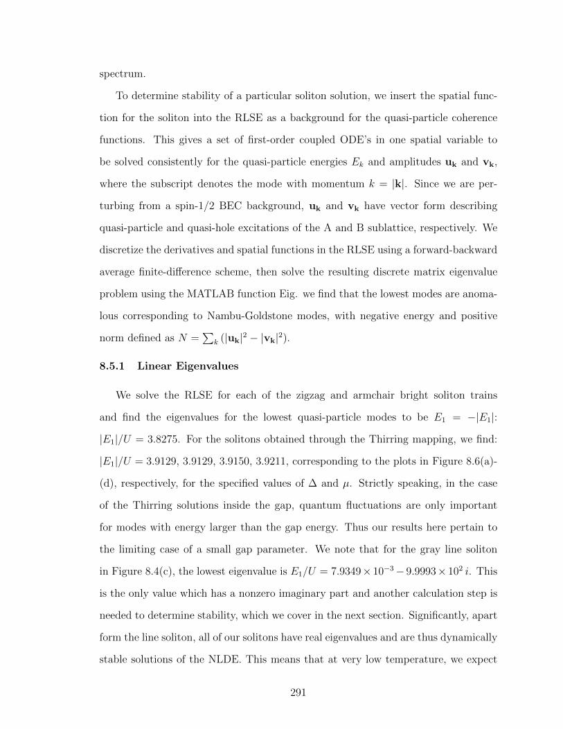
spectrum.

To determine stability of a particular soliton solution, we insert the spatial func-

tion for the soliton into the RLSE as a background for the quasi-particle coherence

functions. This gives a set of first-order coupled ODE’s in one spatial variable to

be solved consistently for the quasi-particle energies Ek and amplitudes uk and vk,

where the subscript denotes the mode with momentum k = |k|. Since we are per-

turbing from a spin-1/2 BEC background, uk and vk have vector form describing

quasi-particle and quasi-hole excitations of the A and B sublattice, respectively. We

discretize the derivatives and spatial functions in the RLSE using a forward-backward

average finite-difference scheme, then solve the resulting discrete matrix eigenvalue

problem using the MATLAB function Eig. we find that the lowest modes are anoma-

lous corresponding to Nambu-Goldstone modes, with negative energy and positive

norm defined as N =∑

k (|uk|2 − |vk|2).

8.5.1 Linear Eigenvalues

We solve the RLSE for each of the zigzag and armchair bright soliton trains

and find the eigenvalues for the lowest quasi-particle modes to be E1 = −|E1|:

|E1|/U = 3.8275. For the solitons obtained through the Thirring mapping, we find:

|E1|/U = 3.9129, 3.9129, 3.9150, 3.9211, corresponding to the plots in Figure 8.6(a)-

(d), respectively, for the specified values of ∆ and µ. Strictly speaking, in the case

of the Thirring solutions inside the gap, quantum fluctuations are only important

for modes with energy larger than the gap energy. Thus our results here pertain to

the limiting case of a small gap parameter. We note that for the gray line soliton

in Figure 8.4(c), the lowest eigenvalue is E1/U = 7.9349× 10−3− 9.9993× 102 i. This

is the only value which has a nonzero imaginary part and another calculation step is

needed to determine stability, which we cover in the next section. Significantly, apart

form the line soliton, all of our solitons have real eigenvalues and are thus dynamically

stable solutions of the NLDE. This means that at very low temperature, we expect

291

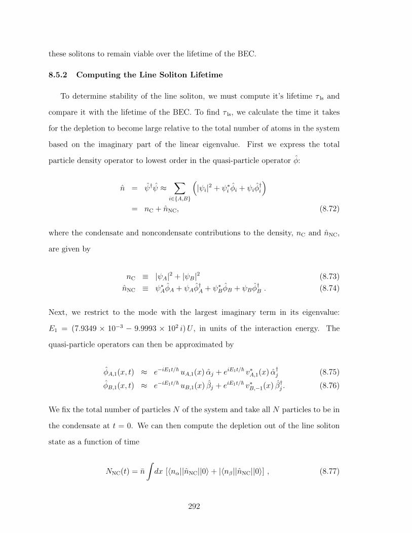
these solitons to remain viable over the lifetime of the BEC.

8.5.2 Computing the Line Soliton Lifetime

To determine stability of the line soliton, we must compute it’s lifetime τ ls and

compare it with the lifetime of the BEC. To find τ ls, we calculate the time it takes

for the depletion to become large relative to the total number of atoms in the system

based on the imaginary part of the linear eigenvalue. First we express the total

particle density operator to lowest order in the quasi-particle operator φ:

n = ψ†ψ ≈∑

i∈A,B

(|ψi|2 + ψ∗i φi + ψiφ

†i

)= nC + nNC, (8.72)

where the condensate and noncondensate contributions to the density, nC and nNC,

are given by

nC ≡ |ψA|2 + |ψB|2 (8.73)

nNC ≡ ψ∗AφA + ψAφ†A + ψ∗BφB + ψBφ

†B . (8.74)

Next, we restrict to the mode with the largest imaginary term in its eigenvalue:

E1 = (7.9349 × 10−3 − 9.9993 × 102 i)U , in units of the interaction energy. The

quasi-particle operators can then be approximated by

φA,1(x, t) ≈ e−iE1t/~ uA,1(x) αj + eiE1t/~ v∗A,1(x) α†j (8.75)

φB,1(x, t) ≈ e−iE1t/~ uB,1(x) βj + eiE1t/~ v∗B,−1(x) β†j . (8.76)

We fix the total number of particles N of the system and take all N particles to be in

the condensate at t = 0. We can then compute the depletion out of the line soliton

state as a function of time

NNC(t) = n

∫dx [〈nα||nNC||0〉+ |〈nβ||nNC||0〉] , (8.77)

292

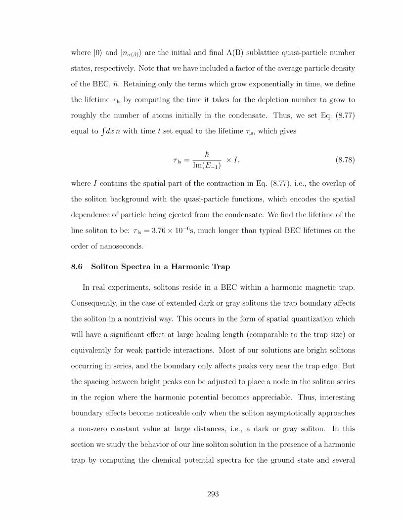
where |0〉 and |nα(β)〉 are the initial and final A(B) sublattice quasi-particle number

states, respectively. Note that we have included a factor of the average particle density

of the BEC, n. Retaining only the terms which grow exponentially in time, we define

the lifetime τ ls by computing the time it takes for the depletion number to grow to

roughly the number of atoms initially in the condensate. Thus, we set Eq. (8.77)

equal to∫dx n with time t set equal to the lifetime τls, which gives

τ ls =~

Im(E−1)× I, (8.78)

where I contains the spatial part of the contraction in Eq. (8.77), i.e., the overlap of

the soliton background with the quasi-particle functions, which encodes the spatial

dependence of particle being ejected from the condensate. We find the lifetime of the

line soliton to be: τ ls = 3.76× 10−6s, much longer than typical BEC lifetimes on the

order of nanoseconds.

8.6 Soliton Spectra in a Harmonic Trap

In real experiments, solitons reside in a BEC within a harmonic magnetic trap.

Consequently, in the case of extended dark or gray solitons the trap boundary affects

the soliton in a nontrivial way. This occurs in the form of spatial quantization which

will have a significant effect at large healing length (comparable to the trap size) or

equivalently for weak particle interactions. Most of our solutions are bright solitons

occurring in series, and the boundary only affects peaks very near the trap edge. But

the spacing between bright peaks can be adjusted to place a node in the soliton series

in the region where the harmonic potential becomes appreciable. Thus, interesting

boundary effects become noticeable only when the soliton asymptotically approaches

a non-zero constant value at large distances, i.e., a dark or gray soliton. In this

section we study the behavior of our line soliton solution in the presence of a harmonic

trap by computing the chemical potential spectra for the ground state and several

293

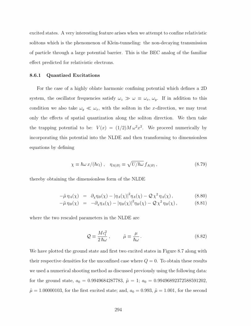
excited states. A very interesting feature arises when we attempt to confine relativistic

solitons which is the phenomenon of Klein-tunneling: the non-decaying transmission

of particle through a large potential barrier. This is the BEC analog of the familiar

effect predicted for relativistic electrons.

8.6.1 Quantized Excitations

For the case of a highly oblate harmonic confining potential which defines a 2D

system, the oscillator frequencies satisfy ωz ω ≡ ωx, ωy. If in addition to this

condition we also take ωy ωx, with the soliton in the x-direction, we may treat

only the effects of spatial quantization along the soliton direction. We then take

the trapping potential to be: V (x) = (1/2)M ω2x2. We proceed numerically by

incorporating this potential into the NLDE and then transforming to dimensionless

equations by defining

χ ≡ ~ω x/(~cl) , ηA(B) ≡√U/~ω fA(B) , (8.79)

thereby obtaining the dimensionless form of the NLDE

−µ ηA(χ) = ∂χηB(χ)− |ηA(χ)|2ηA(χ)−Qχ2 ηA(χ) , (8.80)

−µ ηB(χ) = −∂χηA(χ)− |ηB(χ)|2ηB(χ)−Qχ2 ηB(χ) , (8.81)

where the two rescaled parameters in the NLDE are

Q ≡ Mc2l

2 ~ω, µ ≡ µ

~ω. (8.82)

We have plotted the ground state and first two excited states in Figure 8.7 along with

their respective densities for the unconfined case where Q = 0. To obtain these results

we used a numerical shooting method as discussed previously using the following data:

for the ground state, a0 = 0.9949684287783, µ = 1; a0 = 0.99496892372588591202,

µ = 1.00000103, for the first excited state; and, a0 = 0.993, µ = 1.001, for the second

294

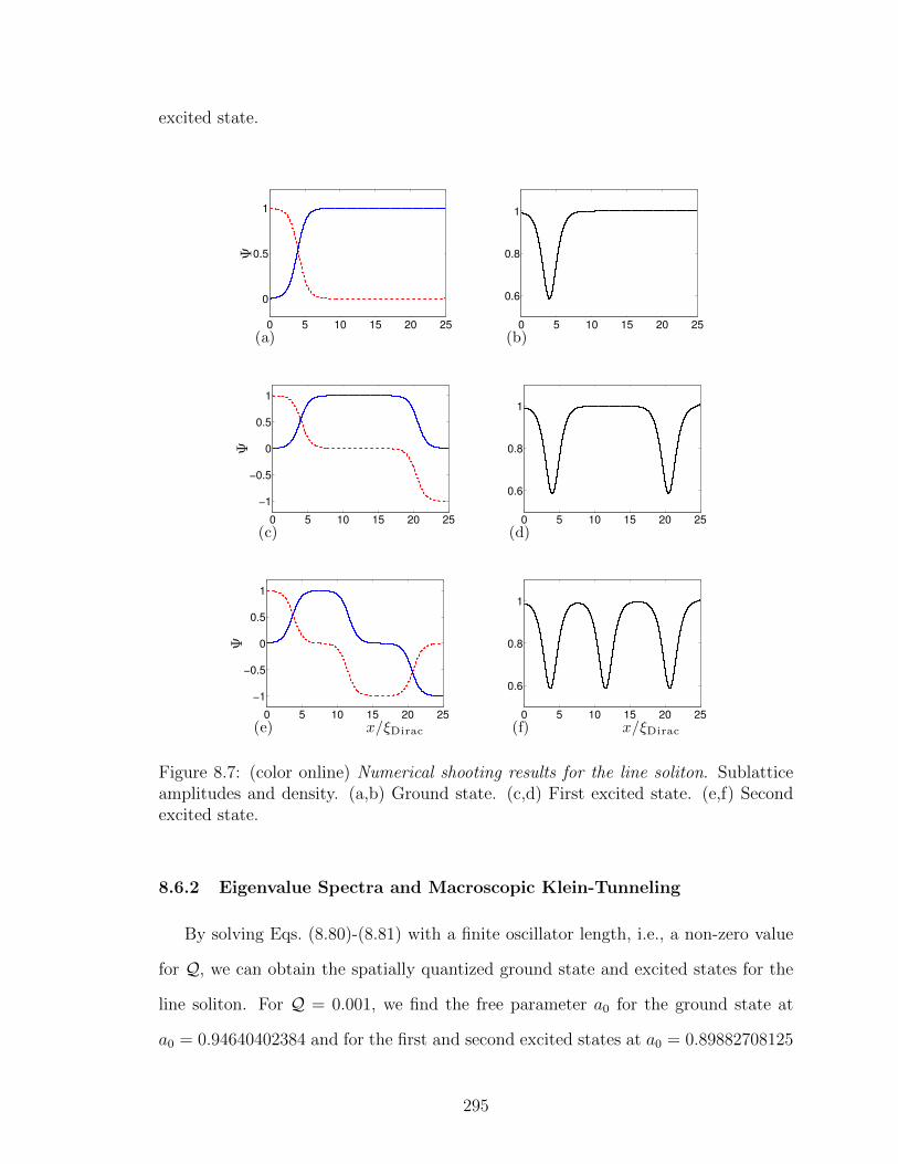
excited state.

0 5 10 15 20 25

0

0.5

1

(a)

Ψ

0 5 10 15 20 25

0.6

0.8

1

(b)

0 5 10 15 20 25

−1

−0.5

0

0.5

1

(c)

Ψ

0 5 10 15 20 25

0.6

0.8

1

(d)

0 5 10 15 20 25

−1

−0.5

0

0.5

1

(e) x/ξDirac

Ψ

0 5 10 15 20 25

0.6

0.8

1

(f) x/ξDirac

Figure 8.7: (color online) Numerical shooting results for the line soliton. Sublatticeamplitudes and density. (a,b) Ground state. (c,d) First excited state. (e,f) Secondexcited state.

8.6.2 Eigenvalue Spectra and Macroscopic Klein-Tunneling

By solving Eqs. (8.80)-(8.81) with a finite oscillator length, i.e., a non-zero value

for Q, we can obtain the spatially quantized ground state and excited states for the

line soliton. For Q = 0.001, we find the free parameter a0 for the ground state at

a0 = 0.94640402384 and for the first and second excited states at a0 = 0.89882708125

295

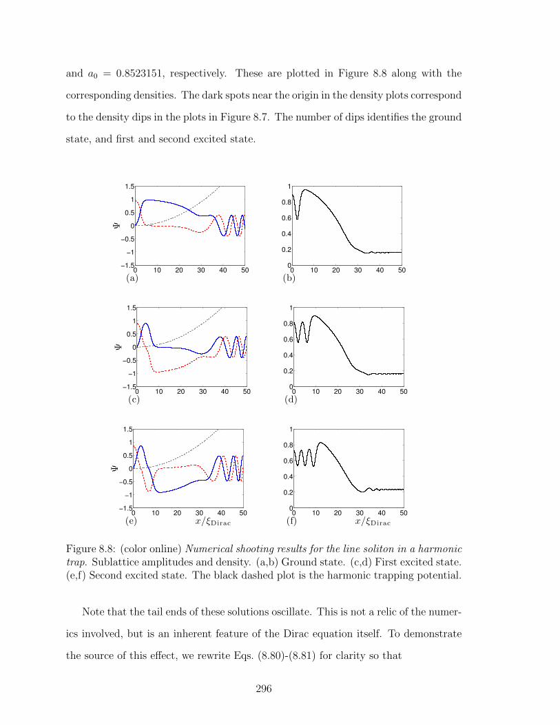
and a0 = 0.8523151, respectively. These are plotted in Figure 8.8 along with the

corresponding densities. The dark spots near the origin in the density plots correspond

to the density dips in the plots in Figure 8.7. The number of dips identifies the ground

state, and first and second excited state.

0 10 20 30 40 50−1.5

−1

−0.5

0

0.5

1

1.5

(a)

Ψ

0 10 20 30 40 500

0.2

0.4

0.6

0.8

1

(b)

0 10 20 30 40 50−1.5

−1

−0.5

0

0.5

1

1.5

(c)

Ψ

0 10 20 30 40 500

0.2

0.4

0.6

0.8

1

(d)

0 10 20 30 40 50−1.5

−1

−0.5

0

0.5

1

1.5

(e) x/ξDirac

Ψ

0 10 20 30 40 500

0.2

0.4

0.6

0.8

1

(f) x/ξDirac

Figure 8.8: (color online) Numerical shooting results for the line soliton in a harmonictrap. Sublattice amplitudes and density. (a,b) Ground state. (c,d) First excited state.(e,f) Second excited state. The black dashed plot is the harmonic trapping potential.

Note that the tail ends of these solutions oscillate. This is not a relic of the numer-

ics involved, but is an inherent feature of the Dirac equation itself. To demonstrate

the source of this effect, we rewrite Eqs. (8.80)-(8.81) for clarity so that

296

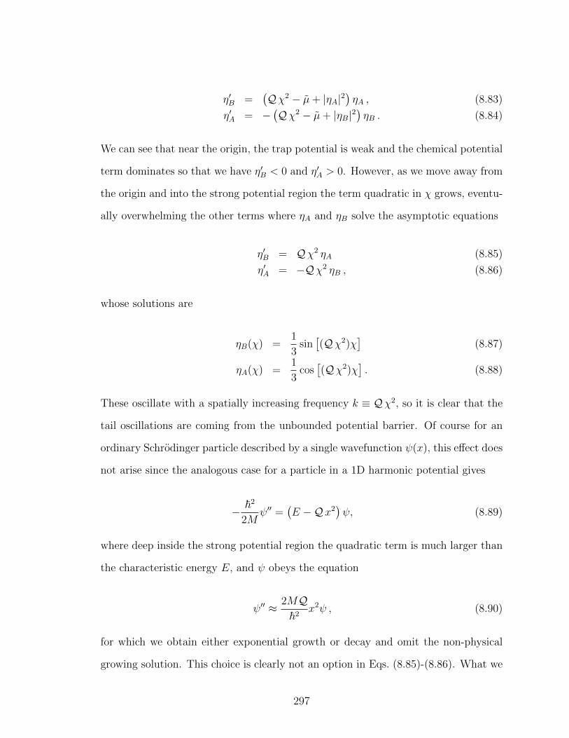
η′B =(Qχ2 − µ+ |ηA|2

)ηA , (8.83)

η′A = −(Qχ2 − µ+ |ηB|2

)ηB . (8.84)

We can see that near the origin, the trap potential is weak and the chemical potential

term dominates so that we have η′B < 0 and η′A > 0. However, as we move away from

the origin and into the strong potential region the term quadratic in χ grows, eventu-

ally overwhelming the other terms where ηA and ηB solve the asymptotic equations

η′B = Qχ2 ηA (8.85)

η′A = −Qχ2 ηB , (8.86)

whose solutions are

ηB(χ) =1

3sin[(Qχ2)χ

](8.87)

ηA(χ) =1

3cos[(Qχ2)χ

]. (8.88)

These oscillate with a spatially increasing frequency k ≡ Qχ2, so it is clear that the

tail oscillations are coming from the unbounded potential barrier. Of course for an

ordinary Schrodinger particle described by a single wavefunction ψ(x), this effect does

not arise since the analogous case for a particle in a 1D harmonic potential gives

− ~2

2Mψ′′ =

(E −Qx2

)ψ, (8.89)

where deep inside the strong potential region the quadratic term is much larger than

the characteristic energy E, and ψ obeys the equation

ψ′′ ≈ 2MQ~2

x2ψ , (8.90)

for which we obtain either exponential growth or decay and omit the non-physical

growing solution. This choice is clearly not an option in Eqs. (8.85)-(8.86). What we

297

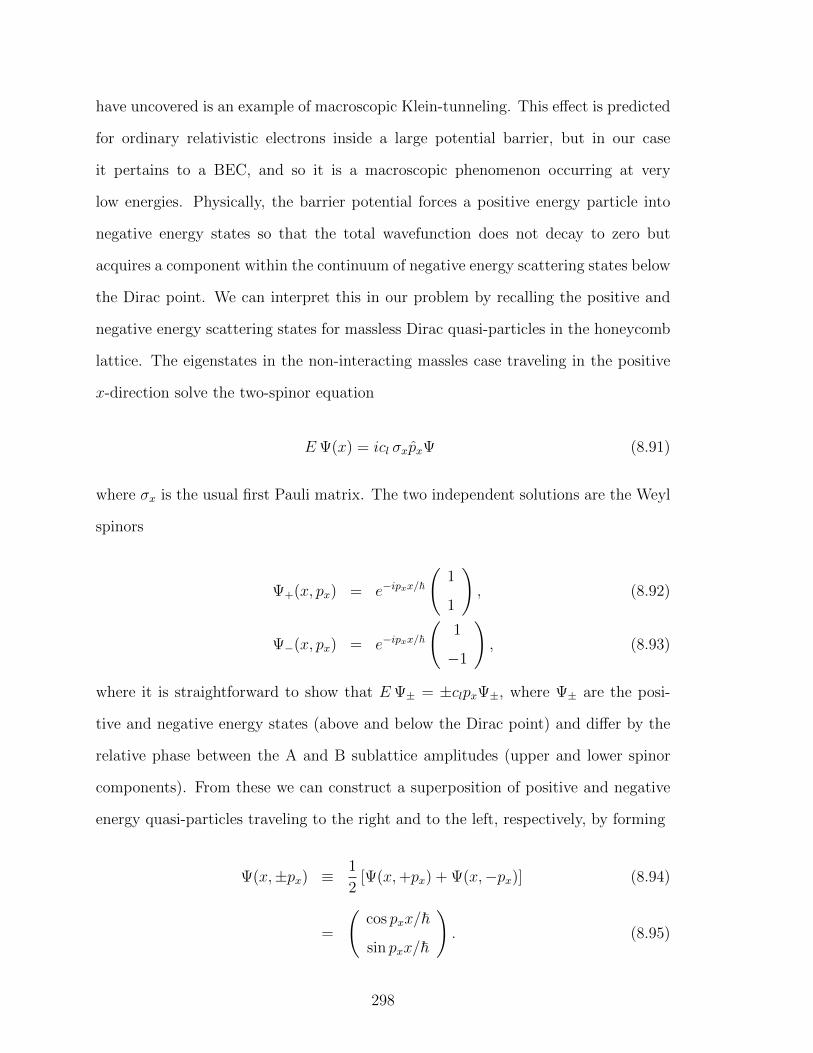
have uncovered is an example of macroscopic Klein-tunneling. This effect is predicted

for ordinary relativistic electrons inside a large potential barrier, but in our case

it pertains to a BEC, and so it is a macroscopic phenomenon occurring at very

low energies. Physically, the barrier potential forces a positive energy particle into

negative energy states so that the total wavefunction does not decay to zero but

acquires a component within the continuum of negative energy scattering states below

the Dirac point. We can interpret this in our problem by recalling the positive and

negative energy scattering states for massless Dirac quasi-particles in the honeycomb

lattice. The eigenstates in the non-interacting massles case traveling in the positive

x-direction solve the two-spinor equation

EΨ(x) = icl σxpxΨ (8.91)

where σx is the usual first Pauli matrix. The two independent solutions are the Weyl

spinors

Ψ+(x, px) = e−ipxx/~

(1

1

), (8.92)

Ψ−(x, px) = e−ipxx/~

(1

−1

), (8.93)

where it is straightforward to show that EΨ± = ±clpxΨ±, where Ψ± are the posi-

tive and negative energy states (above and below the Dirac point) and differ by the

relative phase between the A and B sublattice amplitudes (upper and lower spinor

components). From these we can construct a superposition of positive and negative

energy quasi-particles traveling to the right and to the left, respectively, by forming

Ψ(x,±px) ≡1

2[Ψ(x,+px) + Ψ(x,−px)] (8.94)

=

(cos pxx/~

sin pxx/~

). (8.95)

298

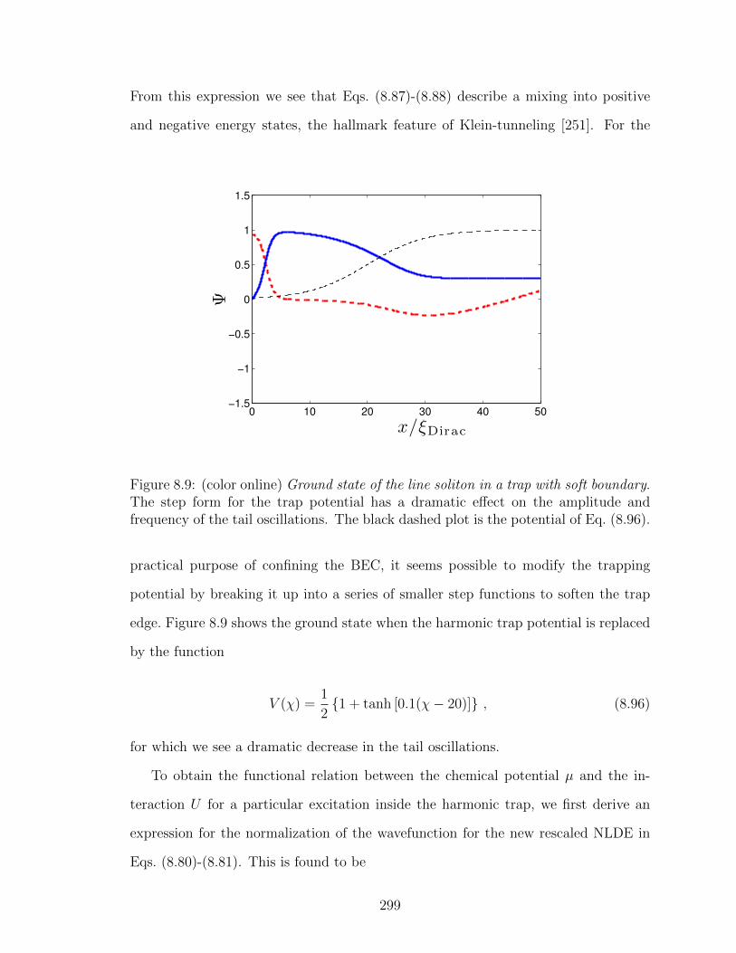
From this expression we see that Eqs. (8.87)-(8.88) describe a mixing into positive

and negative energy states, the hallmark feature of Klein-tunneling [251]. For the

0 10 20 30 40 50−1.5

−1

−0.5

0

0.5

1

1.5

x/ξDirac

Ψ

Figure 8.9: (color online) Ground state of the line soliton in a trap with soft boundary.The step form for the trap potential has a dramatic effect on the amplitude andfrequency of the tail oscillations. The black dashed plot is the potential of Eq. (8.96).

practical purpose of confining the BEC, it seems possible to modify the trapping

potential by breaking it up into a series of smaller step functions to soften the trap

edge. Figure 8.9 shows the ground state when the harmonic trap potential is replaced

by the function

V (χ) =1

21 + tanh [0.1(χ− 20)] , (8.96)

for which we see a dramatic decrease in the tail oscillations.

To obtain the functional relation between the chemical potential µ and the in-

teraction U for a particular excitation inside the harmonic trap, we first derive an

expression for the normalization of the wavefunction for the new rescaled NLDE in

Eqs. (8.80)-(8.81). This is found to be

299

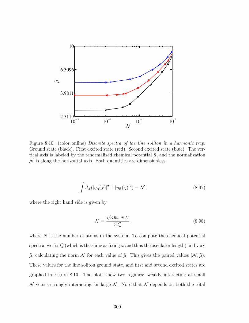
10−3

10−2

10−1

100

2.5119

3.9811

6.3096

10

N

µ

Figure 8.10: (color online) Discrete spectra of the line soliton in a harmonic trap.Ground state (black). First excited state (red). Second excited state (blue). The ver-tical axis is labeled by the renormalized chemical potential µ, and the normalizationN is along the horizontal axis. Both quantities are dimensionless.

∫dχ(|ηA(χ)|2 + |ηB(χ)|2) = N , (8.97)

where the right hand side is given by

N =

√3 ~ωN U

3 t2h, (8.98)

where N is the number of atoms in the system. To compute the chemical potential

spectra, we fixQ (which is the same as fixing ω and thus the oscillator length) and vary

µ, calculating the norm N for each value of µ. This gives the paired values (N , µ).

These values for the line soliton ground state, and first and second excited states are

graphed in Figure 8.10. The plots show two regimes: weakly interacting at small

N versus strongly interacting for large N . Note that N depends on both the total

300

number of atoms and the interaction U , as one would expect. For small N (∼ 10−3),

the solutions correspond to the single-particle bound states of a massless Dirac spinor

trapped inside a harmonic potential. Here the quantization can be seen by noting that

the three states shown in the figure intersect the vertical axis at µ = 2.83, 3.80, 4.88,

or in terms of the oscillator frequency ω: µ = 2.83 ~ω, 3.80 ~ω, 4.88 ~ω, for the ground

state and first two excited states, respectively, which displays approximate integer

multiples n of the energy ~ω: µ ≈ (2.8 + n)~ω. For large N (∼ 1), solutions are

bound gray solitons with spectra characterized by a power law: µ ∝ N α.

8.7 Conclusion

In this article we have presented an exact closed form bright soliton train in

addition to a gray line soliton obtained through a numerical shooting method. We

find a similarity between the analytical bright solitons and those obtained by using

a soliton series expansion technique. Each term in the soliton expansion resembles

the envelope function of the soliton train and suggests the possibility of additional

exact solution. Also, we find that each term in the expansion is an exactly integrable

quantity uniquely associated with a conserved charge, which seems to suggest possible

integrability of the NLDE. A likely fruitful research direction would be a rigorous test

for integrability using a standard analytical method. Solution of the NLDE by inverse

scattering would also lead to a much deeper understanding of its solution space.

By introducing a mass gap into our system we have uncovered a mapping be-

tween the NLDE and the massive Thirring model. The significance of the mapping is

twofold: it allows for a direct incorporation of Thirring solitons into the larger space of

NLDE solutions, while also revealing a completely integrable Poincare invariant sub-

space of the NLDE. From the standpoint of stability, gap solitons are robust objects

due to their isolation from single particle scattering states. In the case of embedded

solitons, we find that all of our bright solitons are stable based on analysis using the

relativistic linear stability equations. However, the line soliton is found to be dynam-

301

ically unstable due to the presence of a complex eigenvalue in its linear spectrum,

with a lifetime of 3.76µs

We have computed the discrete spectra for several bound states of the line soliton

and found two asymptotic regions. One at small interaction where the chemical

potential for excited states differ by a constant multiple of the oscillator energy,

µ ≈ (2.8+n)~ω, and the other limit for large interaction where the chemical potential

obeys a power law: µ ∝ Uα. We have shown that confinement in a harmonic trap leads

to a macroscopic realization of Klein-tunneling and suggests future investigations

extending the full physics of the Klein paradox to the BEC.

Acknowledgments

This material is based in part upon work supported by the National Science Foun-

dation under grant number PHY-1067973. L.D.C. thanks the Alexander von Hum-

boldt foundation and the Heidelberg Center for Quantum Dynamics for additional

support.

8.8 Appendix A: Continuous Spectrum of the NLDE

8.8.1 Four-Spinor Spectrum

Here we present some important details regarding the continuous spectrum of the

nonlinear Dirac operator in the presence of mass gap. The information we present

here provides a context for the solitons described in the main body of this article. We

first consider a BEC that is a macroscopic superposition of excitations at two opposite

Dirac points. In this case, a variety of superpositions of the four-spinor components

are possible. The full NLDE in the chiral representation splits into equations for each

Dirac point:

302

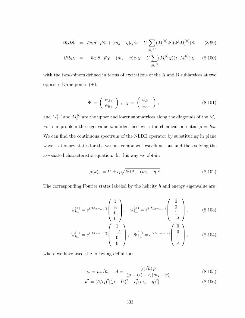
i~ ∂tΦ = ~cl ~σ · ~pΦ + (ms − η)cl Φ− U∑M

(u)i

(M(u)i Φ)(Φ†M

(u)i ) Φ (8.99)

i~ ∂tχ = −~cl ~σ · ~p χ− (ms − η)cl χ− U∑M

(l)i

(M(l)i χ)(χ†M

(l)i )χ , (8.100)

with the two-spinors defined in terms of excitations of the A and B sublattices at two

opposite Dirac points (±),

Φ =

(ψA+

ψB+

), χ =

(ψB−ψA−

), (8.101)

and M(u)i and M

(l)i are the upper and lower submatrices along the diagonals of the Mi.

For our problem the eigenvalue ω is identified with the chemical potential µ = ~ω.

We can find the continuous spectrum of the NLDE operator by substituting in plane

wave stationary states for the various component wavefunctions and then solving the

associated characteristic equation. In this way we obtain

µ(k)± = U ± cl√~2k2 + (ms − η)2 . (8.102)

The corresponding Fourier states labeled by the helicity h and energy eigenvalue are

Ψ(+)h+

= ei (~kx−ω+t)

1A00

, Ψ(+)h−

= ei (~kx−ω+t)

001−A

, (8.103)

Ψ(−)h+

= ei (~kx−ω−t)

1−A00

, Ψ(−)h−

= ei (~kx−ω−t)

001A

, (8.104)

where we have used the following definitions:

ω± = µ±/~, A =(cl/~) p

[(µ− U)− cl(ms − η)], (8.105)

p2 = (~/cl)2[(µ− U)2 − c2l (ms − η)2]. (8.106)

303

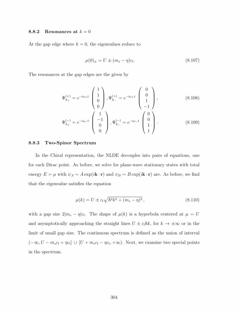
8.8.2 Resonances at k = 0

At the gap edge where k = 0, the eigenvalues reduce to

µ(0)± = U ± (ms − η)cl. (8.107)

The resonances at the gap edges are the given by

Ψ(+)h+

= e−iω+t

1100

,Ψ(+)h−

= e−iω+t

001−1

, (8.108)

Ψ(−)h+

= e−iω−t

1−100

,Ψ(−)h−

= e−iω−t

0011

. (8.109)

8.8.3 Two-Spinor Spectrum

In the Chiral representation, the NLDE decouples into pairs of equations, one

for each Dirac point. As before, we solve for plane-wave stationary states with total

energy E = µ with ψA ∼ A exp(ik · r) and ψB ∼ B exp(ik · r) are. As before, we find

that the eigenvalue satisfies the equation

µ(k) = U ± cl√

~2k2 + (ms − η)2 , (8.110)

with a gap size 2|ms − η|cl. The shape of µ(k) is a hyperbola centered at µ = U

and asymptotically approaching the straight lines U ± cl~k, for k → ±∞ or in the

limit of small gap size. The continuous spectrum is defined as the union of interval

(−∞, U −mscl + ηcl] ∪ [U +mscl − ηcl,+∞). Next, we examine two special points

in the spectrum.

304

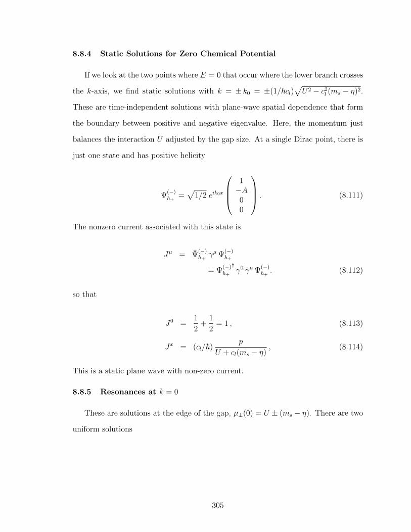
8.8.4 Static Solutions for Zero Chemical Potential

If we look at the two points where E = 0 that occur where the lower branch crosses

the k-axis, we find static solutions with k = ± k0 = ±(1/~cl)√U2 − c2

l (ms − η)2.

These are time-independent solutions with plane-wave spatial dependence that form

the boundary between positive and negative eigenvalue. Here, the momentum just

balances the interaction U adjusted by the gap size. At a single Dirac point, there is

just one state and has positive helicity

Ψ(−)h+

=√

1/2 eik0x

1−A00

. (8.111)

The nonzero current associated with this state is

Jµ = Ψ(−)h+

γµ Ψ(−)h+

= Ψ(−)h+

†γ0 γµ Ψ

(−)h+. (8.112)

so that

J0 =1

2+

1

2= 1 , (8.113)

Jx = (cl/~)p

U + cl(ms − η), (8.114)

This is a static plane wave with non-zero current.

8.8.5 Resonances at k = 0

These are solutions at the edge of the gap, µ±(0) = U ± (ms − η). There are two

uniform solutions

305

Ψ(+)h+

= e−iω+t

1100

, Ψ(−)h+

= e−iω−t

1−100

, (8.115)

where ω± = µ±(0)/~.

306

CHAPTER 9

EFFECTIVE QUANTUM FIELD THEORY FOR BOSONS IN THE

HONEYCOMB LATTICE

L. H. Haddad and Lincoln D. Carr, Physical Review A, to be submitted,

2012.

Abstract

We develop the continuum field theory for bosons near the Dirac points of a

honeycomb lattice and find that the system is described by a relativistic quantum field

theory for Dirac spinors. We derive the effective field theory at the quantum critical

point and find that this is described by a nonlinear Dirac action with additional higher

order terms in the superfluid order parameter and its derivatives. The presence of the

Dirac points result in the characteristic phase differences between the two sublattices

which results in the exact spinor structure for the continuum theory.

307

9.1 Introduction

In the theory of ultracold bosons in a honeycomb lattice, the mean-fields for

bosons defined relative to the Dirac point can be interpreted as quasi-particle fields

propagating on a background which provides an SU(2) Berry phase. Here we use the

Hubbard-Stratonovich formalism to obtain the associated continuum quantum field

theory for bosons. As a preliminary step, we first derive the many-body Hamiltonian

in the lattice by expanding the field operators in terms of Wannier states and focusing

on the geometry of the lattice to arrive at a Hamiltonian for Dirac spinors.

9.2 Microscopic Derivation of the Many-body Hamiltonian for Bosons ina Honeycomb Lattice

9.2.1 First-Order Nearest-Neighbor Hopping

Consider a BEC in a honeycomb optical lattice where we work with characteristic

momentum near the Dirac point. We consider the case of zero particle interactions.

We do this in order to isolate the part of the Hamiltonian which describes low energy

quasi-particle excitations near the Dirac point and show that we arrive at the massless

Dirac Hamiltonian in (2+1)-dimensions. The second quantized Hamiltonian for the

condensate in the lattice is

H =

∫d2rψ†H0ψ, (9.1)

H0 ≡ − ~2

2m∇2 + V (~r) . (9.2)

The field operators ψ = ψ(~r, t) obey bosonic commutation relations in the Heisenberg

picture and V (~r) is the potential of the honeycomb lattice. The goal is to derive the

effective Hamiltonian for quasi-particles interacting with the lattice background. To-

ward this end, we express the many-body wavefunction in terms of a Bloch expansion.

In the tight-binding approximation we can decompose the fields into sums of terms

specific to each lattice site

308

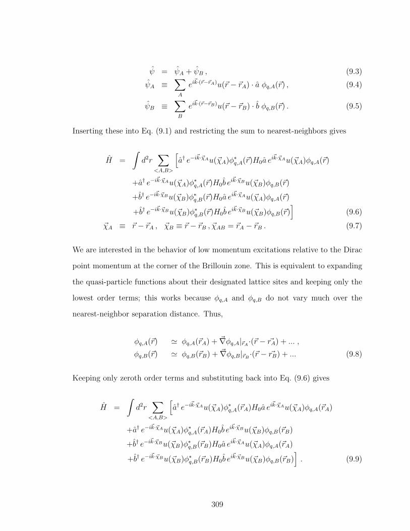
ψ = ψA + ψB , (9.3)

ψA ≡∑A

ei~k·(~r−~rA)u(~r − ~rA) · a φq,A(~r) , (9.4)

ψB ≡∑B

ei~k·(~r−~rB)u(~r − ~rB) · b φq,B(~r) . (9.5)

Inserting these into Eq. (9.1) and restricting the sum to nearest-neighbors gives

H =

∫d2r

∑<A,B>

[a† e−i

~k·~χAu(~χA)φ∗q,A(~r)H0a ei~k·~χAu(~χA)φq,A(~r)

+a† e−i~k·~χAu(~χA)φ∗q,A(~r)H0b e

i~k·~χBu(~χB)φq,B(~r)

+b† e−i~k·~χBu(~χB)φ∗q,B(~r)H0a e

i~k·~χAu(~χA)φq,A(~r)

+b† e−i~k·~χBu(~χB)φ∗q,B(~r)H0b e

i~k·~χBu(~χB)φq,B(~r)]

(9.6)

~χA ≡ ~r − ~rA , ~χB ≡ ~r − ~rB , ~χAB = ~rA − ~rB . (9.7)

We are interested in the behavior of low momentum excitations relative to the Dirac

point momentum at the corner of the Brillouin zone. This is equivalent to expanding

the quasi-particle functions about their designated lattice sites and keeping only the

lowest order terms; this works because φq,A and φq,B do not vary much over the

nearest-neighbor separation distance. Thus,

φq,A(~r) ' φq,A(~rA) + ~∇φq,A|~rA·(~r − ~rA) + ... ,

φq,B(~r) ' φq,B(~rB) + ~∇φq,B|~rB ·(~r − ~rB) + ... (9.8)

Keeping only zeroth order terms and substituting back into Eq. (9.6) gives

H =

∫d2r

∑<A,B>

[a† e−i

~k·~χAu(~χA)φ∗q,A(~rA)H0a ei~k·~χAu(~χA)φq,A(~rA)

+a† e−i~k·~χAu(~χA)φ∗q,A(~rA)H0b e

i~k·~χBu(~χB)φq,B(~rB)

+b† e−i~k·~χBu(~χB)φ∗q,B(~rB)H0a e

i~k·~χAu(~χA)φq,A(~rA)

+b† e−i~k·~χBu(~χB)φ∗q,B(~rB)H0b e

i~k·~χBu(~χB)φq,B(~rB)]. (9.9)

309

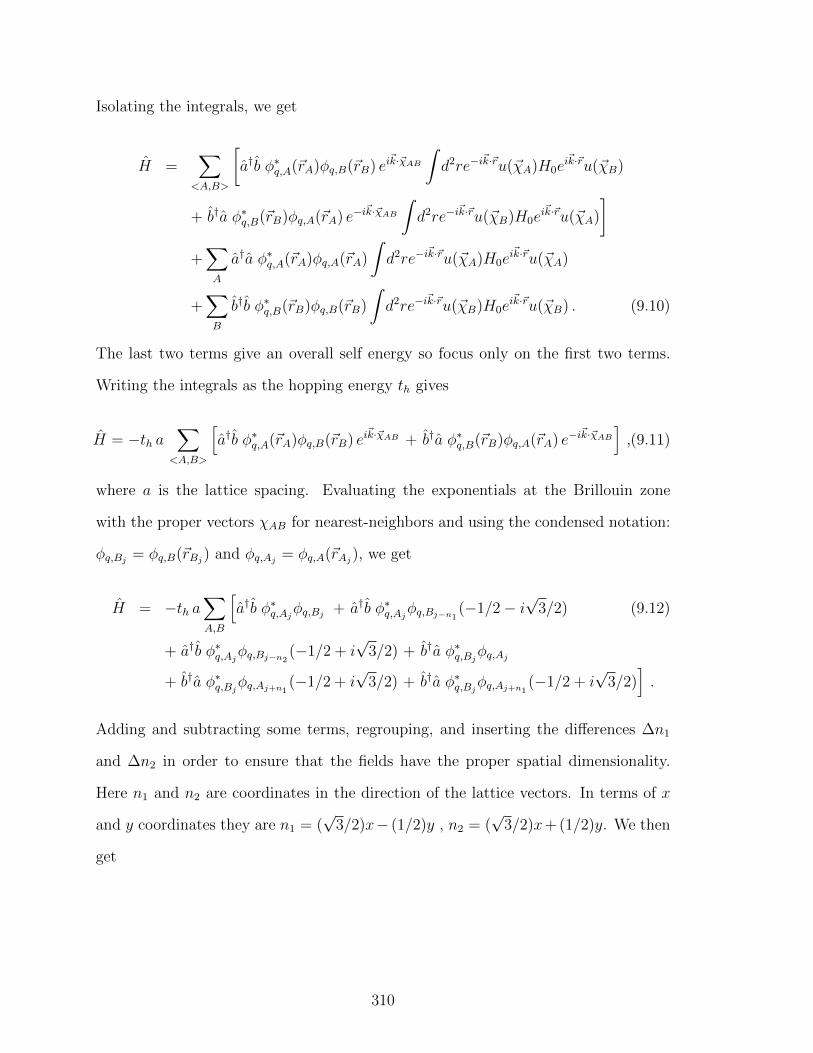
Isolating the integrals, we get

H =∑

<A,B>

[a†b φ∗q,A(~rA)φq,B(~rB) ei

~k·~χAB

∫d2re−i

~k·~ru(~χA)H0ei~k·~ru(~χB)

+ b†a φ∗q,B(~rB)φq,A(~rA) e−i~k·~χAB

∫d2re−i

~k·~ru(~χB)H0ei~k·~ru(~χA)

]+∑A

a†a φ∗q,A(~rA)φq,A(~rA)

∫d2re−i

~k·~ru(~χA)H0ei~k·~ru(~χA)

+∑B

b†b φ∗q,B(~rB)φq,B(~rB)

∫d2re−i

~k·~ru(~χB)H0ei~k·~ru(~χB) . (9.10)

The last two terms give an overall self energy so focus only on the first two terms.

Writing the integrals as the hopping energy th gives

H = −th a∑

<A,B>

[a†b φ∗q,A(~rA)φq,B(~rB) ei

~k·~χAB + b†a φ∗q,B(~rB)φq,A(~rA) e−i~k·~χAB

],(9.11)

where a is the lattice spacing. Evaluating the exponentials at the Brillouin zone

with the proper vectors χAB for nearest-neighbors and using the condensed notation:

φq,Bj= φq,B(~rBj

) and φq,Aj= φq,A(~rAj

), we get

H = −th a∑A,B

[a†b φ∗q,Aj

φq,Bj+ a†b φ∗q,Aj

φq,Bj−n1(−1/2− i

√3/2) (9.12)

+ a†b φ∗q,Ajφq,Bj−n2

(−1/2 + i√

3/2) + b†a φ∗q,Bjφq,Aj

+ b†a φ∗q,Bjφq,Aj+n1

(−1/2 + i√

3/2) + b†a φ∗q,Bjφq,Aj+n1

(−1/2 + i√

3/2)].

Adding and subtracting some terms, regrouping, and inserting the differences ∆n1

and ∆n2 in order to ensure that the fields have the proper spatial dimensionality.

Here n1 and n2 are coordinates in the direction of the lattice vectors. In terms of x

and y coordinates they are n1 = (√

3/2)x− (1/2)y , n2 = (√

3/2)x+ (1/2)y. We then

get

310

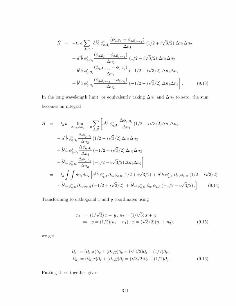
H = −th a∑A,B

[a†b φ∗q,Aj

(φq,Bj− φq,Bj−n1

)

∆n1

(1/2 + i√

3/2) ∆n1∆n2

+ a†b φ∗q,Aj

(φq,Bj− φq,Bj−n2

)

∆n2

(1/2− i√

3/2) ∆n1∆n2

+ b†a φ∗q,Bj

(φq,Aj+n1− φq,Aj

)

∆n1

(−1/2 + i√

3/2) ∆n1∆n2

+ b†a φ∗q,Bj

(φq,Aj+n2− φq,Aj

)

∆n2

(−1/2− i√

3/2) ∆n1∆n2

]. (9.13)

In the long wavelength limit, or equivalently taking ∆n1 and ∆n2 to zero, the sum

becomes an integral

H = −th a lim∆n1,∆n2 → 0

∑A,B

[a†b φ∗q,Aj

∆φq,Bj

∆n1

(1/2 + i√

3/2)∆n1∆n2

+ a†b φ∗q,Aj

∆φq,Bj

∆n2

(1/2− i√

3/2) ∆n1∆n2

+ b†a φ∗q,Bj

∆φq,Aj

∆n1

(−1/2 + i√

3/2) ∆n1∆n2

+ b†a φ∗q,Bj

∆φq,Aj

∆n2

(−1/2− i√

3/2) ∆n1∆n2

]= −th

∫ ∫dn1dn2

[a†b φ∗q,A ∂n1φq,B (1/2 + i

√3/2) + a†b φ∗q,A ∂n2φq,B (1/2− i

√3/2)

+ b†a φ∗q,B ∂n1φq,A (−1/2 + i√

3/2) + b†a φ∗q,B ∂n2φq,A (−1/2− i√

3/2) .]

(9.14)

Transforming to orthogonal x and y coordinates using

n1 = (1/√

3)x− y , n2 = (1/√

3)x+ y

⇒ y = (1/2)(n2 − n1) , x = (√

3/2)(n1 + n2), (9.15)

we get

∂n1 = (∂n1x)∂x + (∂n1y)∂y = (√

3/2)∂x − (1/2)∂y ,

∂n2 = (∂n2x)∂x + (∂n2y)∂y = (√

3/2)∂x + (1/2)∂y . (9.16)

Putting these together gives

311

H = −th a∫ ∫

dx dya†b φ∗q,A [(

√3/2)∂x − (1/2)∂y]φq,B (1/2 + i

√3/2)

+ a†b φ∗q,A [(√

3/2)∂x + (1/2)∂y]φq,B (1/2− i√

3/2)

+ b†a φ∗q,B [(√

3/2)∂x − (1/2)∂y]φq,A (−1/2 + i√

3/2)

+ b†a φ∗q,B [(√

3/2)∂x + (1/2)∂y]φq,A (−1/2− i√

3/2). (9.17)

Finally, after multiplying out and recombining the terms, and rotating the coordinate

system, we obtain the expression

H = −th a(√

3/2)

∫ ∫dx dy

[a†b φ∗q,A (∂xφq,B − i∂yφq,B) + b†a φ∗q,B (∂xφq,A + i∂yφq,A)

]= −th(

√3/2)

∫ ∫dx dy

[ψ†A (∂xψB − i∂yψB) + ψ†B (∂xψA + i∂yψA)

]. (9.18)

This is the second quantized Dirac Hamiltonian for one pseudospin valley of the

honeycomb lattice. By going through the same steps for the opposite corner of the

Brillouin zone we get the usual 4-spinor Hamiltonian for a free massless particle:

H = −i th a(√

3/2)

∫d2r ψ† (γµ∂µ) ψ , (9.19)

where

ψ ≡

a φq,A+

b φq,B+

b φq,B−a φq,A−

. (9.20)

We can see that the inclusion of higher order corrections through Eq. (9.8) will intro-

duce symmetry breaking terms reflecting a greater resolution of the lattice structure.

For example, adding another term would result in a Hamiltonian with an additional

quadratic term in the spatial derivatives which a quadratic correction to the linear

Dirac dispersion.

312

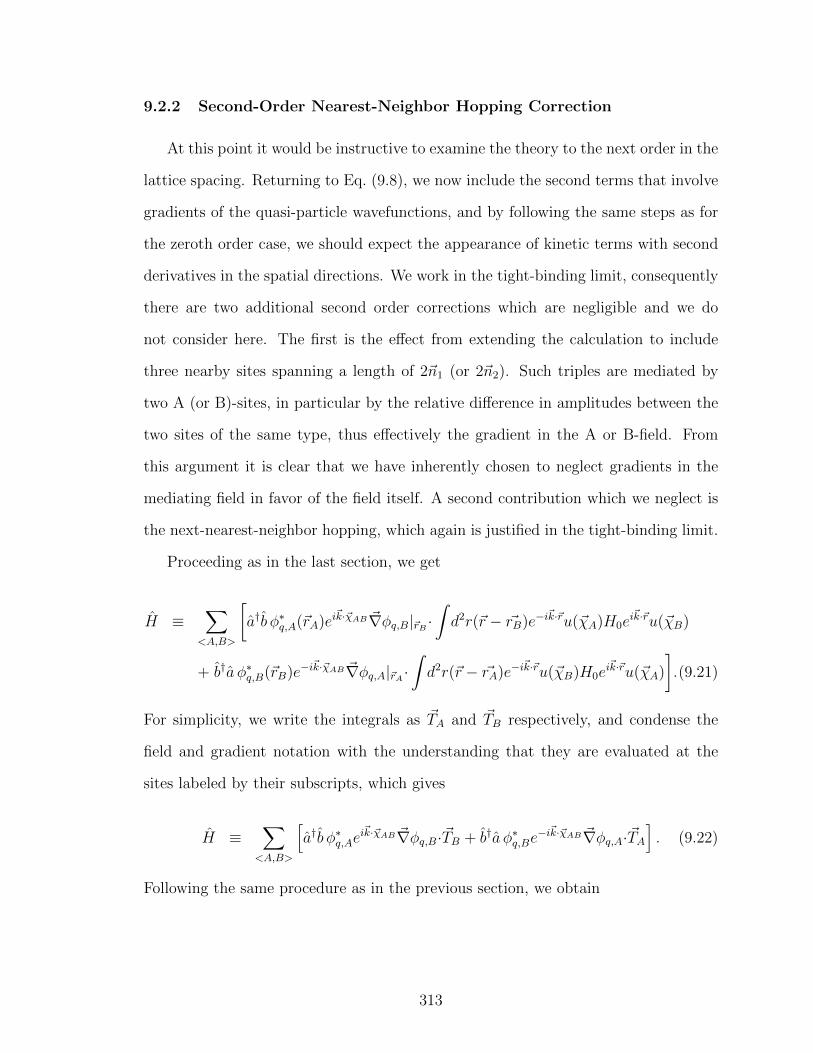
9.2.2 Second-Order Nearest-Neighbor Hopping Correction

At this point it would be instructive to examine the theory to the next order in the

lattice spacing. Returning to Eq. (9.8), we now include the second terms that involve

gradients of the quasi-particle wavefunctions, and by following the same steps as for

the zeroth order case, we should expect the appearance of kinetic terms with second

derivatives in the spatial directions. We work in the tight-binding limit, consequently

there are two additional second order corrections which are negligible and we do

not consider here. The first is the effect from extending the calculation to include

three nearby sites spanning a length of 2~n1 (or 2~n2). Such triples are mediated by

two A (or B)-sites, in particular by the relative difference in amplitudes between the

two sites of the same type, thus effectively the gradient in the A or B-field. From

this argument it is clear that we have inherently chosen to neglect gradients in the

mediating field in favor of the field itself. A second contribution which we neglect is

the next-nearest-neighbor hopping, which again is justified in the tight-binding limit.

Proceeding as in the last section, we get

H ≡∑

<A,B>

[a†b φ∗q,A(~rA)ei

~k·~χAB ~∇φq,B|~rB ·∫d2r(~r − ~rB)e−i

~k·~ru(~χA)H0ei~k·~ru(~χB)

+ b†a φ∗q,B(~rB)e−i~k·~χAB ~∇φq,A|~rA·

∫d2r(~r − ~rA)e−i

~k·~ru(~χB)H0ei~k·~ru(~χA)

].(9.21)

For simplicity, we write the integrals as ~TA and ~TB respectively, and condense the

field and gradient notation with the understanding that they are evaluated at the

sites labeled by their subscripts, which gives

H ≡∑

<A,B>

[a†b φ∗q,Ae

i~k·~χAB ~∇φq,B·~TB + b†a φ∗q,Be−i~k·~χAB ~∇φq,A·~TA

]. (9.22)

Following the same procedure as in the previous section, we obtain

313

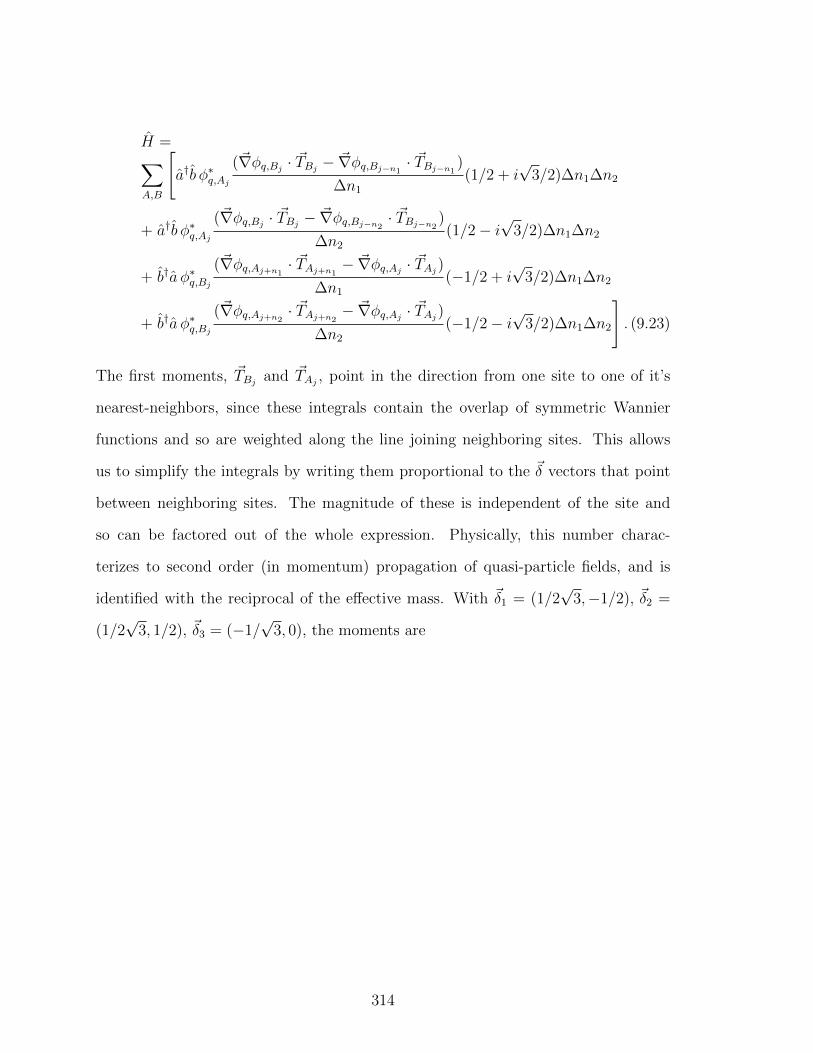
H =∑A,B

[a†b φ∗q,Aj

(~∇φq,Bj· ~TBj

− ~∇φq,Bj−n1· ~TBj−n1

)

∆n1

(1/2 + i√

3/2)∆n1∆n2

+ a†b φ∗q,Aj

(~∇φq,Bj· ~TBj

− ~∇φq,Bj−n2· ~TBj−n2

)

∆n2

(1/2− i√

3/2)∆n1∆n2

+ b†a φ∗q,Bj

(~∇φq,Aj+n1· ~TAj+n1

− ~∇φq,Aj· ~TAj

)

∆n1

(−1/2 + i√

3/2)∆n1∆n2

+ b†a φ∗q,Bj

(~∇φq,Aj+n2· ~TAj+n2

− ~∇φq,Aj· ~TAj

)

∆n2

(−1/2− i√

3/2)∆n1∆n2

]. (9.23)

The first moments, ~TBjand ~TAj

, point in the direction from one site to one of it’s

nearest-neighbors, since these integrals contain the overlap of symmetric Wannier

functions and so are weighted along the line joining neighboring sites. This allows

us to simplify the integrals by writing them proportional to the ~δ vectors that point

between neighboring sites. The magnitude of these is independent of the site and

so can be factored out of the whole expression. Physically, this number charac-

terizes to second order (in momentum) propagation of quasi-particle fields, and is

identified with the reciprocal of the effective mass. With ~δ1 = (1/2√

3,−1/2), ~δ2 =

(1/2√

3, 1/2), ~δ3 = (−1/√

3, 0), the moments are

314

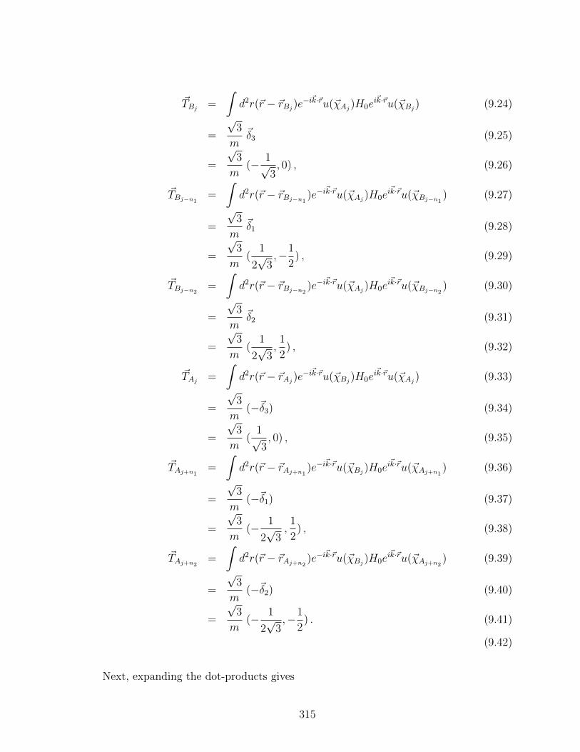
~TBj=

∫d2r(~r − ~rBj

)e−i~k·~ru(~χAj

)H0ei~k·~ru(~χBj

) (9.24)

=

√3

m~δ3 (9.25)

=

√3

m(− 1√

3, 0) , (9.26)

~TBj−n1=

∫d2r(~r − ~rBj−n1

)e−i~k·~ru(~χAj

)H0ei~k·~ru(~χBj−n1

) (9.27)

=

√3

m~δ1 (9.28)

=

√3

m(

1

2√

3,−1

2) , (9.29)

~TBj−n2=

∫d2r(~r − ~rBj−n2

)e−i~k·~ru(~χAj

)H0ei~k·~ru(~χBj−n2

) (9.30)

=

√3

m~δ2 (9.31)

=

√3

m(

1

2√

3,1

2) , (9.32)

~TAj=

∫d2r(~r − ~rAj

)e−i~k·~ru(~χBj

)H0ei~k·~ru(~χAj

) (9.33)

=

√3

m(−~δ3) (9.34)

=

√3

m(

1√3, 0) , (9.35)

~TAj+n1=

∫d2r(~r − ~rAj+n1

)e−i~k·~ru(~χBj

)H0ei~k·~ru(~χAj+n1

) (9.36)

=

√3

m(−~δ1) (9.37)

=

√3

m(− 1

2√

3,1

2) , (9.38)

~TAj+n2=

∫d2r(~r − ~rAj+n2

)e−i~k·~ru(~χBj

)H0ei~k·~ru(~χAj+n2

) (9.39)

=

√3

m(−~δ2) (9.40)

=

√3

m(− 1

2√

3,−1

2) . (9.41)

(9.42)

Next, expanding the dot-products gives

315

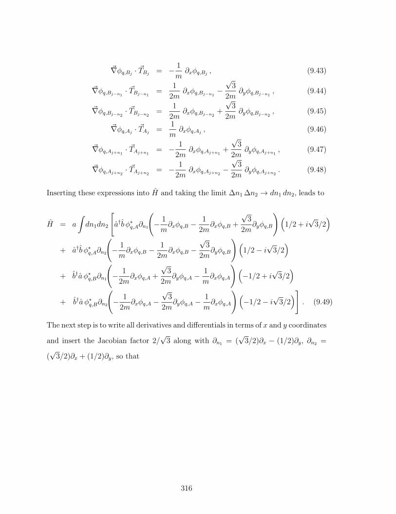
~∇φq,Bj· ~TBj

= − 1

m∂xφq,Bj

, (9.43)

~∇φq,Bj−n1· ~TBj−n1

=1

2m∂xφq,Bj−n1

−√

3

2m∂yφq,Bj−n1

, (9.44)

~∇φq,Bj−n2· ~TBj−n2

=1

2m∂xφq,Bj−n2

+

√3

2m∂yφq,Bj−n2

, (9.45)

~∇φq,Aj· ~TAj

=1

m∂xφq,Aj

, (9.46)

~∇φq,Aj+n1· ~TAj+n1

= − 1

2m∂xφq,Aj+n1

+

√3

2m∂yφq,Aj+n1

, (9.47)

~∇φq,Aj+n2· ~TAj+n2

= − 1

2m∂xφq,Aj+n2

−√

3

2m∂yφq,Aj+n2

. (9.48)

Inserting these expressions into H and taking the limit ∆n1 ∆n2 → dn1 dn2, leads to

H = a

∫dn1dn2

[a†b φ∗q,A∂n1

(− 1

m∂xφq,B −

1

2m∂xφq,B +

√3

2m∂yφq,B

)(1/2 + i

√3/2)

+ a†b φ∗q,A∂n2

(− 1

m∂xφq,B −

1

2m∂xφq,B −

√3

2m∂yφq,B

)(1/2− i

√3/2)

+ b†a φ∗q,B∂n1

(− 1

2m∂xφq,A +

√3

2m∂yφq,A −

1

m∂xφq,A

)(−1/2 + i

√3/2)

+ b†a φ∗q,B∂n2

(− 1

2m∂xφq,A −

√3

2m∂yφq,A −

1

m∂xφq,A

)(−1/2− i

√3/2)]

. (9.49)

The next step is to write all derivatives and differentials in terms of x and y coordinates

and insert the Jacobian factor 2/√

3 along with ∂n1 = (√

3/2)∂x − (1/2)∂y, ∂n2 =

(√

3/2)∂x + (1/2)∂y, so that

316

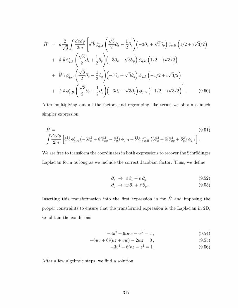
H = a2√3

∫dxdy

2m

[a†b φ∗q,A

(√3

2∂x −

1

2∂y

)(−3∂x +

√3∂y

)φq,B

(1/2 + i

√3/2)

+ a†b φ∗q,A

(√3

2∂x +

1

2∂y

)(−3∂x −

√3∂y

)φq,B

(1/2− i

√3/2)

+ b†a φ∗q,B

(√3

2∂x −

1

2∂y

)(−3∂x +

√3∂y

)φq,A

(−1/2 + i

√3/2)

+ b†a φ∗q,B

(√3

2∂x +

1

2∂y

)(−3∂x −

√3∂y

)φq,A

(−1/2− i

√3/2)]

. (9.50)

After multiplying out all the factors and regrouping like terms we obtain a much

simpler expression

H = (9.51)∫dxdy

2m

[a†b φ∗q,A

(−3∂2

x + 6i∂2xy − ∂2

y

)φq,B + b†a φ∗q,B

(3∂2

x + 6i∂2xy + ∂2

y

)φq,A

].

We are free to transform the coordinates in both expressions to recover the Schrodinger

Laplacian form as long as we include the correct Jacobian factor. Thus, we define

∂x → u ∂x + v ∂y (9.52)

∂y → w ∂x + z ∂y . (9.53)

Inserting this transformation into the first expression in for H and imposing the

proper constraints to ensure that the transformed expression is the Laplacian in 2D,

we obtain the conditions

−3u2 + 6iuw − w2 = 1 , (9.54)

−6uv + 6i(uz + vw)− 2wz = 0 , (9.55)

−3v2 + 6ivz − z2 = 1 . (9.56)

After a few algebraic steps, we find a solution

317

u = i7

3

√3

4, (9.57)

v = −2 , (9.58)

w =

√3

4, (9.59)

z = i , (9.60)

and the Jacobian factor for this transformation is −3√

4/3. The constraints for the

second expression in H are

3u2 + 6iuw + w2 = 1 , (9.61)

6uv + 6i(uz + vw) + 2wz = 0 , (9.62)

3v2 + 6ivz + z2 = 1 , (9.63)

where, after more algebra, we find that

u =7

3

√3

4, (9.64)

v = −2i , (9.65)

w = i

√3

4, (9.66)

z = 1 . (9.67)

The Jacobian factor here is 3√

4/3. Finally, the transformed Hamiltonian is

H =√

3a

∫dxdy

m

(−a†b φ∗q,A~∇2φq,B + b†a φ∗q,B ~∇2φq,A

). (9.68)

For the special mode where φq,B = φq,A, we obtain the form

H =√

3a

∫d2r

[ψ†A

(−~2~∇2

m

)ψB + ψ†B

(~2~∇2

m

)ψA

]. (9.69)

This gives the second order correction to the Hamiltonian for long-wavelength ex-

citations corresponding to the second order expansion of the dispersion relation for

318

the upper and lower branches of the Dirac cone. The many-body Hamiltonian up to

second-order in spatial derivatives can be expressed in condensed notation. Including

the result from the previous gives

H = −i∫d2r ψ†

(~cl σ · p +

√3

mσy p2

)ψ . (9.70)

9.3 Continuum Quantum Field Theory

We can determine the structure of the low energy excitations of the insulating

phase by the usual quantum field theory technique. First we introduce the superfluid

order parameters as before but now we allow it vary in two (continuous) spatial

dimensions as well as time: ψ(r, τ). The path integral form of the Euclidean partition

function near the SF-MI phase transition is

Z =

∫Dci(τ)Dc∗i (τ) exp

(−∫ 1/T

0

dτL), (9.71)

L =∑i

(c∗i~∂τci − µc∗i ci +

1

2Uc∗i c

∗i cici

)− J

∑<i,j>

(c∗i cj + c∗jci

), (9.72)

where the indices i, j are short hand for the ith and jth lattice vectors ri and rj

respectively and c and c∗ are the corresponding bosonic fields. Decoupling the hopping

term as before by the standard Hubbard-Stratanovich transformation by introducing

the auxiliary field ψi(τ) into Z which gives

Z =

∫Dci(τ)Dc∗i (τ)Dψi(τ)Dψ∗i (τ) exp

(−∫ 1/T

0

dτL′), (9.73)

L′ =∑i

(c∗i~∂τci − µc∗i ci +

1

2Uc∗i c

∗i cici − ψic∗i − ψ∗i ci

)+∑<i,j>

ψ∗i J−1ij ψj . (9.74)

Note that the dependence on the Euclidean time τ is implied. The usual process

involves integrating over ci and c∗i and then performing a derivative expansion in the

319

superfluid fields ψi to obtain the low energy, long wavelength, effective action. To

connect to the Dirac theory, we still must translate the action to the edge of the

Brillouin zone before performing the integral over the ci. Resetting the zero-point for

the fields to the Dirac point requires the addition of an extra phase in the hopping

terms which comes from the background. Also, we must make the sublattice structure

explicit in the hopping terms so that L′ becomes

L′ =∑

<r,r′>∈A,B

(c∗r~∂τcr − µc∗rcr +

1

2Uc∗rc

∗rcrcr − eiθrr′ψrJ

−1rr′ c

∗r′ − e−iθr′rψ∗r′J−1

rr′ cr

)

+∑<r,r′>

eiθrr′ψ∗rJ−1rr′ψr′ , (9.75)

where eiθrr′ is the directed background phase between nearest-neighbor sites coming

from the Bloch wave expansion at the Dirac point of the lattice. The notation in the

first summation refers to the A sublattice and B sublattice vector spaces. Next, we

factor the partition function

Z =

∫Dψi(τ)Dψ∗i (τ) exp

[−th

~

∫dτ

∑<r,r′>

eiθrr′ψ∗rψr′

]

×∫Dci(τ)Dc∗i (τ)exp

−th~

∫dτ

∑<r,r′>∈A,B

(−eiθrr′ψrc

∗r′ − e−iθr′rψ∗r′cr

)×exp

−L0[c, c∗]

~

, (9.76)

where we have reduced the nearest-neighbor transition matrix to J−1rr′ = th and the

action composed purely of Mott fields is

L0[c, c∗] =

∫dτ∑

r∈A,B

c∗r

(~∂τ − µ+

1

2Uc∗rcr

)cr . (9.77)

The functional integral over the Mott fields in the second line of Z is just the ex-

pectation value of the exponential containing the cross-terms of Mott and superfluid

320

fields weighted by the exponential of the action S0:

Z =

∫Dψi(τ)Dψ∗i (τ) exp

[−th

~

∫dτ

∑<r,r′>

eiθrr′ψ∗rψr′

]

× 〈exp

−th~

∫dτ

∑<r,r′>∈A,B

(−eiθrr′ψrc

∗r′ − e−iθr′rψ∗r′cr

)〉0. (9.78)

To evaluate this expression, we follow the usual cumulant expansion prescription but,

since the Mott fields do not acquire an expectation value in the ground state, all odd

power correlators vanish which simplifying the expansion

〈exp(M)〉even0 ≈ exp

[1

2〈M2〉0 + 〈M4〉0 −

1

4〈M2〉20 + ...

]. (9.79)

Then the effective action up to second order in the superfluid field ψ and ψ∗ is

Leff[ψ, ψ∗] = −th~∑<r,r′>

∫dτ eiθrr′ψ∗rψr′

+∑<r,r′>

∫dτ

[t2h

2~2〈(eiθrr′ψrc

∗r′ + e−iθr′rψ∗r′cr

)2〉0 +t4h~4〈(eiθrr′ψrc

∗r′ + e−iθr′rψ∗r′cr

)4〉0

− t4h4~4〈(eiθrr′ψrc

∗r′ + e−iθr′rψ∗r′cr

)2〉20]. (9.80)

Next, we note the following properties of the two-point and four-point functions

321

〈cr(τ)c∗r′(τ′)〉0 = δ(r− r′)〈c(τ)c∗(τ ′)〉0 , (9.81)

〈c∗r(τ)c∗r′(τ′)〉0 = 〈cr(τ)cr′(τ

′)〉0 = 0 , (9.82)

〈cr(τ)cr′(τ′)c∗r′′(τ

′′)c∗r′′′(τ′′′)〉0 = (9.83)

δ(r− r′)δ(r′ − r′′)δ(r′′ − r′′′)〈c(τ)c(τ ′)c∗(τ ′′)c∗(τ ′′′)〉0 , (9.84)

〈c∗r(τ)c∗r′(τ′)c∗r′′(τ

′′)c∗r′′′(τ′′′)〉0 = 0 , (9.85)

〈c∗r(τ)c∗r′(τ′)c∗r′′(τ

′′)cr′′′(τ′′′)〉0 = 0 , (9.86)

〈c∗r(τ)cr′(τ′)cr′′(τ

′′)cr′′′(τ′′′)〉0 = 0 , (9.87)

〈cr(τ)cr′(τ′)cr′′(τ

′′)cr′′′(τ′′′)〉0 = 0 . (9.88)

To compute the two-point function we introduce the imaginary time ordering

operator T and express the answer in terms of an operator expression so that we can

connect to our previous work:

〈c(τ)c∗(τ ′)〉0 = 〈T[c(τ)c†(τ ′)

]〉0 (9.89)

= θ(τ − τ ′) 〈c(τ)c†(τ ′)〉0 + θ(τ ′ − τ)〈c†(τ ′)c(τ)〉0 , (9.90)

and in the second line we have expressed the time-ordered result in terms of the

Heavyside functions. These expressions can be computed exactly by using the result

that we found before for the ground state energy:

E(0)g =

1

2Ug (g − 1) − µ g , (9.91)

with g the number of particles in the ground state. The problem reduces to the simple

formula

322

〈 τ ′ , g | c(τ ′) c†(τ) | τ , g 〉

= (g + 1) 〈 0 , g + 1 | exp[(E

(0)g+1 − E(0)

g

)τ ′/~

]· exp

[−(E

(0)g+1 − E(0)

g

)τ/~]| 0 , g + 1 〉

= (g + 1) exp[−(E

(0)g+1 − E(0)

g

)(τ − τ ′)/~

], (9.92)

so that

〈c(τ)c∗(τ ′)〉0 = θ(τ − τ ′) (g + 1) exp[−(E

(0)g+1 − E(0)

g

)(τ − τ ′)/~

]+θ(τ ′ − τ) g exp

[(E

(0)g−1 − E(0)

g

)(τ − τ ′)/~

], (9.93)

keeping in mind that

E(0)g+1 − E(0)

g = g U − µ , (9.94)

E(0)g−1 − E(0)

g = (g − 1)U − µ , (9.95)

then

〈c(τ)c∗(τ ′)〉0 = θ(τ − τ ′)(g + 1) exp [− (gU − µ) (τ − τ ′)/~]

+ θ(τ ′ − τ)gexp [(gU − U − µ) (τ − τ ′)/~] . (9.96)

For the four-point function, we can use Wick’s theorem to reduce it to sums of prod-

ucts of two-point functions and then evaluate these using our previous results:

323

〈T [c(τ)c(τ ′)c∗(τ ′′)c∗(τ ′′′)]〉0 (9.97)

= 〈T [c(τ)c∗(τ ′′′)]〉0 〈T [c(τ ′)c∗(τ ′′)]〉0+〈T [c(τ)c∗(τ ′′)]〉0 〈T [c(τ ′)c∗(τ ′′′)]〉0

= θ(τ − τ ′′′) (g + 1) exp [− (gU − µ) (τ − τ ′′′)/~]

+ θ(τ ′′′ − τ) g exp [− (gU − U − µ) (τ − τ ′′′)/~]×θ(τ ′ − τ ′′) (g + 1) exp [− (gU − µ) (τ ′ − τ ′′)/~]

+ θ(τ ′′ − τ ′) g exp [− (gU − U − µ) (τ ′ − τ ′′)/~]+ θ(τ − τ ′′) (g + 1) exp [− (gU − µ) (τ − τ ′′)/~]

+ θ(τ ′′ − τ) g exp [− (gU − U − µ) (τ − τ ′′)/~]×θ(τ ′ − τ ′′′) (g + 1) exp [− (gU − µ) (τ ′ − τ ′′′)/~]

+ θ(τ ′′′ − τ ′) g exp [− (gU − U − µ) (τ ′ − τ ′′′)/~] . (9.98)

Using these results and forming discrete derivatives in the fist summation of the

effective action, we can then take the continuum limit, also, we note that the phase

difference between nearest-neighbor sites have the property that φ ≡ θrr′ = − θr′rwhere we now call the phase difference φ to avoid confusing it with the Heavyside

step function. We obtain:

Leff[ψ, ψ∗] = −th~

∫dr dτ i [ψ∗A(r, τ)(∂x − i∂y)ψB(r, τ) + ψ∗B(r, τ)(∂x + i∂y)ψA(r, τ)]

+∑

i∈A,B

∫dr dτ

[th2~

∫dτ ′ ei2φ ψi(r, τ)ψ∗i (r, τ

′)〈T [c(τ)c∗(τ ′)]〉0

+t4h~4

∫dτ ′ dτ ′′ dτ ′′′ ei4φ ψ∗i (r, τ

′′)ψ∗i (r, τ′′′)ψi(r, τ

′)ψi(r, τ)

× 〈T [c(τ)c∗(τ ′′′)]〉0 〈T [c(τ ′)c∗(τ ′′)]〉0 + 〈T [c(τ)c∗(τ ′′)]〉0

×〈T [c(τ ′)c∗(τ ′′′)]〉0 −t4h

4~4

∫dτ ′ ei2φ ψi(r, τ)ψ∗i (r, τ

′)〈T [c(τ)c∗(τ ′)]〉02].

(9.99)

Next, we rewrite the integral with respect to τ ′ in the second line above:

324

∫dτ ′ ei2φ ψi(r, τ)ψ∗i (r, τ

′)〈T [c(τ)c∗(τ ′)]〉0

= ei2φψi(r, τ)

∫ τ

0

dτ ′ ψ∗i (r, τ′) (g + 1) exp [− (gU − µ) (τ − τ ′)/~]

+ ei2φψi(r, τ)

∫ ∞τ

dτ ′ ψ∗i (r, τ′) g exp [(gU − U − µ) (τ − τ ′)/~]

= ei2φ[

(g + 1)

(gU − µ)+

g

(gU − U − µ)

]~|ψi(r, τ)|2

− ei2φ[

(g + 1)

(gU − µ)2− g

(gU − U − µ)2

]~2ψ∗i (r, τ)∂τψi(r, τ) +O(~3), (9.100)

where the second equality comes from integrating by parts twice with respect to

τ ′ and dropping an overall constant. Continuing this process produces higher order

derivatives and powers of the superfluid order parameter which, in the low energy and

low momentum approximation, justify the truncation. Computing all other terms and

combining the sublattice fields ψi in spinor form Ψ ≡ (ψA, ψB)T , the effective action

takes the final form

Leff[Ψ, Ψ] = (9.101)

−∫dr dτ

Ψ∂τΨ + icl Ψ (σ · ∇) Ψ +u

2

∑i∈A,B

|ψi|4 + r|Ψ|2 + κ1|∂τΨ|2 + κ2|∇Ψ|2 .

Here we have defined Ψ ≡ (Ψ∗)T . The first three terms comprise the classical action

for the nonlinear Dirac equation, the fourth term is a quadratic chemical potential

where r = 0 gives the condition for the second order superfluid-insulator transition,

and the last two quadratic terms describe second sound for the superfluid. Note

that the final term comes from the next order correction to the gradient describing

departure from linear dispersion at the Dirac point. This is computed in detail in

the next section. Notably, Eq.(9.102) is the Lagrangian that describes the strongly

interacting critical quantum field theory at the Dirac point of the honeycomb lattice.

Notice that in the coefficients of the higher order terms, th occurs as a modified

325

hopping parameter t′h ≡ ei2φth. This has the effect of weighting transitions in the

direction of the lattice momentum K by a factor of (1 + i√

3) and in the opposite

direction of K by a factor of (1−i√

3). The imaginary parts of these weights represent

the effect of the background condensate on the hopping terms that appear at the level

of the Hamiltonian. We can see their effects by noting that the induced transition

amplitude from lattice site i to site j in the direction of K is obtained by taking the

expectation value after exponentiating the imaginary parts of the hopping terms

T (i→ j) = 〈ni − 1, nj + 1|exp[−i(i√

3th)b†jbi(t− t0)/~

]|ni, nj〉 − 1

≈ (t− t0)th√

3n1/2i (nj + 1)1/2/2~ , (9.102)

while for the reverse process we get:

T (j → i) ≈ −(t− t0)th√

3n1/2j (ni + 1)1/2/2~ . (9.103)

As we would expect, the imaginary terms induce gains and losses of particles for tran-

sitions along K and opposite K respectively. Yet, it is crucial to note that the phase

transition depends on |ei2φth|, so that what we have described is just an interpretation

of the phase as a mean-field effect that accounts for higher order interactions with

the background condensate.

9.4 Conclusion

We have obtained the continuum quantum field theory for bosons near the Dirac

point, and found that it has the same form as that of relativistic interacting Dirac

spinors, but with two additional interaction terms corresponding to second sound in

the superfluid, one proportional to the square of the time derivative and the other

proportional the square of the gradient of the field. The equation of motion for the

corresponding single-particle states is the nonlinear Dirac equation, with additional

terms second order in the space-time derivatives. Together, these extra second order

326

terms are identical to the Klein-Gordon momentum terms. This last feature points

to the interesting prospect of a possible redefinition of fields to obtain a relativistic

theory of interacting fermions and bosons. Several modifications to our results offer

the possibility of investigating more elaborate field theories. For example, by including

mass gaps and nearest neighbor interactions, which can be tuned to be attractive or

repulsive, may lead to other interesting field theories near criticality such as Gross-

Neveu, Chern-Simons, Kogut-Susskind, and Yukawa theory, in addition to low energy

supersymmetric theories.

327

CHAPTER 10

CONCLUSIONS AND OUTLOOK

In this thesis we have derived the nonlinear Dirac equation, a new mean-field

theory which describes bosons in a 2D honeycomb lattice analogous to the nonlin-

ear Schrodinger equation for general BECs in 3D. In addition, we have derived the

relativistic linear stability equations (RLSE), the relativistic generalization of the

Bogoliubov-de Gennes equations. We have obtained localized solutions of the NLDE

which include bright and gray solitons, topological and non-topological vortices, half-

quantum vortices, and skyrmion textures. Although similar solutions have been stud-

ied in ordinary BECs confined only by a magnetic trap, our solutions exhibit a Dirac

spinor structure due to the presence of the honeycomb optical lattice. Thus, we ob-

tain solitons, vortices, and textures with a Dirac spinor structure sharing features in

common with both spinor BECs and particle physics models.

From the point of view of experimental realization, we have clearly defined all the

physical parameters of our theory through a systematic reduction from the usual 3D

BEC parameters down to the effective 2D lattice at long-wavelengths. The constraints

are clearly established and a workable range of values is determined for all of our

parameters. We have fully described the necessary steps to construct the lattice and

transfer the BEC to any desired vortex configuration while maintaining the system in

a metastable state. In addition, discrete spectra for relativistic vortices give a global

perspective for vortex energies as functions of the particle interaction. A significant

result of our findings is that most of the soliton solutions are perfectly stable while

most vortex lifetimes are on the order of or greater than the BEC lifetime. Together,

these results provide a formal prescription for realizing relativistic vortices in the

laboratory.

329

On the theory side, we have characterized the low energy quantum fluctuations of

all of our solutions by developing a new theory of relativistic quasi-particles contained

in the RLSE. The RLSE describe propagation of pseudospin-1/2 quasi-particles sim-

ilar to the case of graphene pseudospin valley excitations. However, we go beyond

the standard graphene picture by considering the effect of tuning a bosonic contact

interaction with positive s-wave scattering. By solving for the coherence factors we

find that tuning the interaction U upward gradually changes the character of quasi-

particle excitations from pseudospin-1/2 to pseudospin-0 or 1, i.e., to a singlet or

triplet state. More precisely stated, for U √

3 πtha/R, where th is the hopping

energy, a the lattice constant, and R the condensate radius, quasi-particles are dis-

tinct and uncorrelated pseudospin-1/2 states: the lattice spin-valley structure is only

weakly affected by particle interactions. On the other hand, when U √

3πtha/R,

quasi-particles are highly correlated into pairs with aligned or anti-aligned pseudospin.

When considering a typical vortex solution of the NLDE in the mean- field picture,

quantum fluctuations appear as either bound states (fluctuations of the vortex) or

free scattering states (fluctuations of the ambient background). Bound states are

localized within one or two healing lengths of the vortex core and deplete the vortex

by introducing equal admixtures of particles and holes,

We have analyzed the 1D NLDE, obtained experimentally by making the trap size

small in one of the planar directions, which amounts to setting one spatial derivative

to zero. The 1D case offers an opportunity to focus on the question of integrability,

since the most common integrable systems are 1D models. One approach to prov-

ing integrability of a system is to find a reparametrization, or mapping, to another

known integrable model. By doing so we gain insight into the original system and

possibly new solutions. Using the complete four-spinor NLDE with mass gap as a

starting point, which provides a large parameter space to work with, we have found

a reparametrization which maps the imaginary and real parts of A and B sublat-

330

tice wavefunctions to the two independent spinor functions of the massive Thirring

model. As a consequence, we were able to apply the map in reverse and obtain new

soliton solutions for the massive 1D NLDE. The Thirring parameters are directly

related to the mass gap parameter, chemical potential, and interaction strength in

the NLDE picture. Integrability of the Thirring model is well known and has been

studied extensively, which suggests a direction for further investigations of the 1D

NLDE.

We have found a series solution of the 1D NLDE, when the NLDE spinor is

parametrized by Ψ(x) = η(x) [cosϕ(x), sinϕ(x)]T . Our method expands the envelope

function η(x) in powers of the quantity cosϕ(x)4 + sinϕ(x)4, which appears in the

NLDE after incorporating our ansatz, and we obtain the expansion coefficients by

matching. For the internal parameter function ϕ(x), we arrive at a power series with

each term a differential equation for ϕ(x) containing either a positive or negative

power of cosϕ(x)4 + sinϕ(x)4. Such terms are integrable and lead to an infinite

number of conserved quantities for each term in the series. Interestingly, the terms

in our series expansion match solutions which we have found by another independent

method. This discussion points to symmetries of the 1D NLDE which exist and

warrant deeper investigation. In particular, the conserved charges that we have found

strongly suggest integrability and an underlying Lax-pair structure.

The NLDE allows for a large variety of vortex solutions, which may be classified

according to how the internal degrees of freedom evolve under spatial rotations. Thus

a thorough classification of our solutions into topological classes would provide a

comparison with similar topological vortices in the area of spinor BECs. Spinor

BECs are well established, where topological structures such as skyrmion textures

are commonplace. One advantage of accessing atomic hyperfine degrees of freedom

within the honeycomb lattice setting, is that this would allow for the same freedom as

in the case of spinor BECs, but with the Schrodinger differential operator replaced by

331

the Dirac operator. In principle, the combination of internal and lattice symmetries

would lead to unique nonlinear structures not yet observed in cold atomic gases.

Another possible area to investigate is the use of mixtures of more than one

atomic species. Combined with a spin-dependent lattice, as we have discussed in

Chapters 6 and 7, this approach offers another way to simulate relativistic mean–

field theories. Specifically, the advantage of using this method lies in tuning the

lattice parameters so that one type of atom experiences the lattice potential, while

the other atoms experience only the harmonic trap. The corresponding continuum

mean- field theory would contain Dirac spinors, as we have shown in this thesis,

as well as excitations which behave according to the usual Schrodinger paradigm.

Furthermore, the inclusion of interactions between the different atom types, would

result in a theory of interacting Dirac spinors where interactions are mediated by the

additional bosons, which could simulate a semiclassical electromagnetic field.

In Chapter 9, we established the full many-body continuum field theory for bosons.

We use the Hubbard-Sratonovich method for mean-field decomposition at the insula-

tor/superfluid boundary, and we expect that an analogous technique which includes

nearest neighbor interactions will result in terms which mix the spinor components,

in contrast to the case of on-site interactions. By tuning the relative strengths and

signs of these interactions, we may be able to simulate a large number of relativistic

field theories, since many such theories differ mainly by the specific ways in which the

interactions couple the spinor components. By including in this picture the various

mass gaps, which we have explored in Chapter 8, we obtain a large parameter space

to work with, including four gap parameters and two types of interactions. This offers

an intriguing low-energy scenario: by tuning the relative strengths and signs of mass

gap parameters, on-site interactions, and nearest-neighbor interactions, we expect to

see phase transitions connecting several different nonlinear Dirac theories.

332

Bose-Einstein condensates in honeycomb lattices offer the opportunity for more

detailed investigations into fundamental questions around non-equilibrium BECs. In

this thesis, particularly in Chapters 6 and 7, we have shown that it is possible to

create a BEC at inherently metastable points in the honeycomb lattice, namely at

the Dirac points. Combined with our lifetime and stability analyses, we have set

the ground for questions such as non-equilibrium phase fluctuations, growth of the

condensate fraction, and turbulence in non-equilibrium systems.

333

REFERENCES CITED

[1] M. H. Anderson, J. R. Ensher, M. R. Matthews, C. E. Wieman, and E. A.Cornell. Observation of Bose-Einstein condensation in a dilute atomic vapor.Science, 269:198–201, 1995.

[2] K. B. Davis, M.-O. Mewes, M. R. Andrews, N. J. van Druten, D. S. Durfee,D. M. Kurn, and W. Ketterle. Bose-Einstein condensation in a gas of sodiumatoms. Phys. Rev. Lett., 75:3969–3973, 1995.

[3] C. C. Bradley, C. A. Sackett, J. J. Tollett, and R. G. Hulet. Evidence of Bose-Einstein condensation in an atomic gas with attractive interactions. Phys. Rev.Lett., 75:1687–1690, 1995.

[4] A. J. Leggett. Bose-Einstein condensation in the alkali gases: Some fundamentalconcepts. Rev. Mod. Phys., 73:307–356, 2001.

[5] I. Bloch, J. Dalibard, and W. Zwerger. Many-body physics with ultracold gases.Rev. Mod. Phys., 80:885–964, 2008.

[6] F. Dalfovo, S. Giorgini, L. P. Pitaevskii, and S. Stringari. Theory of Bose-Einstein condensation in trapped gases. Rev. Mod. Phys., 71:463–512, 1999.

[7] C. Pethick and H. Smith. Bose-Einstein Condensation in Dilute Gases. Cam-bridge University Press, 2002.

[8] M. Lewenstein, A. Sanpera, V. Ahufinger, B. Damski, A. Sen De, and U. Sen.Ultracold atomic gases in optical lattices: mimicking condensed matter physicsand beyond. Advances in Physics, 56:243, 2007.

[9] C. J. Myatt, E. A. Burt, R. W. Ghrist, E. A. Cornell, and C. E. Wieman. Pro-duction of two overlapping Bose-Einstein condensates by sympathetic cooling.Phys. Rev. Lett., 78:586–589, 1997.

[10] D. M. Stamper-Kurn, M. R. Andrews, A. P. Chikkatur, S. Inouye, H. J. Miesner,J. Stenger, and W. Ketterle. Optical confinement of a Bose-Einstein condensate.Phys. Rev. Lett., 80:2027–2030, 1998.

[11] A. I. Safonov, S. A. Vasilyev, I. S. Yasnikov, I. I. Lukashevich, and S. Jaakkola.Observation of quasicondensate in two-dimensional atomic hydrogen. Phys.Rev. Lett., 81:4545–4548, 1998.

335

[12] R. Kaiser, C. Westbrook, and F. David, editors. Coherent atomic matter waves.EDP Sciences and Springer-Verlag, Les Ulis, France and Berlin, Germany, 2001.

[13] J. H. Denschlag, J. E. Simsarian, H. Haffner, C. McKenzie, A. Browaeys,D. Cho, K. Helmerson, S. L. Rolston, and W. D. Phillips. A Bose-Einsteincondensate in an optical lattice. J. Phys. B, 35:3095–3110, 2002.

[14] A. Jacob, P. Ohberg, G. Juzeliunas, and L. Santos. Cold atom dynamics innon-Abelian gauge fields. Appl. Phys. B, 89:439–445, 2008.

[15] C. Wu and S. Das Sarma. The px,y-orbital counterpart of graphene: Cold atomsin the honeycomb optical lattice. Phys. Rev. B, 77:235107, 2008.

[16] S. L. Zhu, B. Wang, and L.-M. Duan. Simulation and detection of Dirac fermionswith cold atoms in an optical lattice. Phys. Rev. Lett., 98:260402, 2007.

[17] B. Anderson. Experiments with vortices in superfluid atomic gases. Journal ofLow Temperature Physics, 161:574–602, 2010.

[18] L.-K. Lim, A. Hemmerich, and C. M. Smith. Artificial staggered magnetic fieldfor ultracold atoms in optical lattices. Phys. Rev. A, 2010.

[19] P. G. Kevrekidis, D. J. Frantzeskakis, and R. Carretero-Gonzalez. EmergentNonlinear Phenomena in Bose-Einstein Condensates. Springer-Verlag, Berlin,2008.

[20] M. J. Ablowitz and Y. Zhu. Evolution of bloch-mode envelopes in two-dimensional generalized honeycomb lattices. Phys. Rev. A, 82:013840, 2010.

[21] Z. H. Musslimani, M. Segev, and D. N. Christodoulides. Multicomponent two-dimensional solitons carrying topological charges. Opt. Lett., 25:61–63, 2000.

[22] F. Lederer, G. I. Stegeman, D. N. Christodoulides, G. Assanto, M. Segev, andY. Silberberg. Discrete solitons in optics. Phys. Rep., 463:1–126, 2008.

[23] W. Zhang, C. A. Sackett, and R. G. Hulet. Optical detection of a Bardeen-Cooper-Schrieffer phase transition in a trapped gas of fermionic atoms. Phys.Rev. A, 60:504–507, 1999.

[24] G. M. Bruun and C. W. Clark. Detection of the BCS transition of a trappedFermi gas. J. Phys. B: At. Mol. Opt. Phys., 33:3953, 2000.

[25] D. S. Petrov, C. Salomon, and G. V. Shlyapnikov. Weakly bound dimers offermionic atoms. Phys. Rev. Lett., 93:090404, 2004.

336

[26] P. G. Saffman. Vortex Dynamics. Cambridge University Press, The Pitt Build-ing, Trumpington Street, Cambridge CB2 1RP, 1992.

[27] F. Dalfovo, S. Giorgini, L. P. Pitaevskii, and S. Stringari. Theory of Bose-Einstein condensation in trapped gases. Rev. Mod. Phys., 71:463–512, 1999.

[28] A. L. Fetter and A. A. Svidzinsky. Stability of a vortex in a rotating trappedBose-Einstein condensate. Phys. Rev. Lett., 84:5919–23, 2000.

[29] A. L. Fetter and A. A. Svidzinsky. Vortices in a trapped dilute Bose-Einsteincondensate. J. Phys.: Condens. Matter, 13:R135, 2001.

[30] E. H. Lieb and R. Seiringer. Proof of Bose-Einstein condensation for dilutetrapped gases. Phys. Rev. Lett., 88:170409, 2002.

[31] E. H. Lieb, R. Seiringer, J. P. Solovej, and Jakob Yngvason. The Mathematicsof the Bose Gas and its Condensation. Springer, 2005.

[32] Z. Chen and B. Wu. Bose-Einstein condensate in a honeycomb optical lattice:Fingerprint of superfluidity at the Dirac point. Phys. Rev. Lett., 107:065301,2011.

[33] G.E. Volovick. The Universe in a Helium Droplet. Oxford University Press,Great Clarendon Street, Oxford OX2 6DP, 2003.

[34] W.G. Unruh and R. Schutzhold, editors. Quantum analogues: from phase tran-sitions to black holes and cosmology. Springer-Verlag, 233 Spring Street, NewYork, NY 10013, 2007.

[35] C. Chin, R. Grimm, P. Julienne, and E. Tiesinga. Feshbach resonances inultracold gases. Rev. Mod. Phys., 82:1225–1286, 2010.

[36] M. Greiner, O. Mandel, T. Esslinger, T. W. Hansch, and I. Bloch. Quantumphase transition from a superfluid to a Mott insulator in a gas of ultracoldatoms. Nature, 415:39–44, 2002.

[37] L. Tarruell, D. Greif, T. Uehlinger, G. Jotzu, and T. Esslinger. Creating,moving and merging dirac points with a Fermi gas in a tunable honeycomblattice. Nature, 483:302, 2012.

[38] A. E. Leanhardt, Y. Shin, D. Kielpinski, D. E. Pritchard, and W. Ketterle.Coreless vortex formation in a spinor Bose-Einstein condensate. Phys. Rev.Lett., 90:140403, 2003.

337

[39] M. R. Matthews, B. P. Anderson, P. C. Haljan, D. S. Hall, C. E. Wieman, andE. A. Cornell. Vortices in a Bose-Einstein condensate. Phys. Rev. Lett., 83:2498–2501, 1999.

[40] J. E. Williams and M J. Holland. Preparing topological states of a Bose-Einsteincondensate. Nature, 401:568–572, 1999.

[41] V. Schweikhard, I. Coddington, S. Tung P. Engels, and E. A. Cornell. Vortexlattice dynamics in rotating spinor Bose-Einstein condensates. Phys. Rev. Lett.,2004.

[42] K. Kasamatsu, M. Tsubota, and M. Ueda. Spin textures in rotating two-component Bose-Einstein condensates. Phys. Rev. A, 71:043611, 2005.

[43] Y. Kawaguchi, M. Nitta, and M. Ueda. Knots in a spinor Bose-Einstein con-densate. Phys. Rev. Lett., 100:180403, 2008.

[44] Y. Kawaguchi and M. Ueda. Symmetry classification of spinor Bose-Einsteincondensates. Phys. Rev. A, 84:053616, 2011.

[45] D. Durfee and W. Ketterle. Experimental studies of Bose-Einstein condensation.Opt. Express, 2:299–313, 1998.

[46] S. Inouye, D. M. Stamper-Kurn, H.-J. Miesner, A. P. Chikkatur, and W. Ket-terle. Spin domains in ground-state Bose-Einstein condensates. Nature, 396:345–348, 1998.

[47] T.-L. Ho. Spinor Bose condensates in optical traps. Phys. Rev. Lett., 81:742–745, 1998.

[48] A. K. Geim and K. S. Novoselov. The rise of graphene. Nature Materials, 6:183–191, 2007.

[49] M. Katsnelson and K. S. Novoselov. Graphene: New bridge between condensedmatter physics and quantum electrodynamics. Solid State Commun., 143, 2007.

[50] P. R. Wallace. The band structure of graphite. Phys. Rev., 71:622–634, 1947.

[51] V. Gusynin, S. Sharapov, and J. Carbotte. Ac conductivity of graphene: fromtight-binding model to 2+1-dimensional quantum electrodynamics. Interna-tional Journal of Modern Physics B, 2007.

338

[52] L. H. Haddad and L. D. Carr. The nonlinear Dirac equation in Bose-Einsteincondensates: Foundation and symmetries. Physica D: Nonlinear Phenomena,238:1413–1421, 2009.

[53] J. C. Slonczewski and P. R. Weiss. Band structure of graphite. Phys. Rev., 109:272–279, 1958.

[54] M. I. Katsnelson and K. S. Novoselov. Graphene: New bridge between con-densed matter physics and quantum electrodynamics. Solid State Commun.,143:3–13, 2007.

[55] E. Antonyan, J. A. Harvey, S. Jensen, and D. Kutasov. NJL and QCD fromstring theory. e-print arXiv:hep-th/0604017, 2006.

[56] E. Antonyan, J. A. Harvey, and D. Kutasov. The Gross-Neveu model fromstring theory. e-print arXiv:hep-th/0608149v1, 2006.

[57] N. N. Bogoliubov. On the theory of superfluidity. J. Phys. (USSR), 11:23–32,1947.

[58] E. P. Gross. Structure of a quantized vortex in a Bose system. Nuovo Cimento,20:454, 1961.

[59] L.P. Pitaevskii. Vortex lines in an imperfect Bose gas. Sov. Phys. JETP, 13:451, 1961.

[60] Y. Castin and R. Dum. Low-temperature Bose-Einstein condensates in time-dependent traps: Beyond the U(1) symmetry-breaking approach. Phys. Rev.A, 57:3008–3021, 1998.

[61] N. P. Proukakis and K. Burnett. Generalized mean fields for trapped Bose-Einstein condensates. J. Res. Natl. Inst. Stand. Technol., 101:457, 1996.

[62] G. L. Alfimov, P. G. Kevrekidis, V. V. Konotop, and M. Salerno. Wannier func-tions analysis of the nonlinear Schrodinger equation with a periodic potential.Phys. Rev. E, 66:046608, 2002.

[63] V. M. Perez-Garcia, N. G. Berloff, P. G. Kevrekidis, and V. V. Konotop. Nonlin-ear phenomena in degenerate quantum gases. Physica D: Nonlinear Phenomena,238:1289, 2009.

[64] V. I. Yukalov. Cold bosons in optical lattices. Laser Physics, 19:1, 2009.

339

[65] S. Sachdev. Quantum Phase Transitions. Cambridge University Press, TheEdinburgh Building, Cambridge CB2 8RU, UK, 1999.

[66] A. L. Fetter. Nonuniform states of an imperfect Bose gas. Annals of Physics,70:67–101, 1972.

[67] H. T. C. Stoof, D. B. M. Dickerscheid, and K. Gubbels. Ultracold QuantumFields. Springer, 2009.

[68] L. D. Carr, Charles W. Clark, and W. P Reinhardt. Stationary solutions of theone-dimensional nonlinear Schrodinger equation. I. Case of repulsive nonlinear-ity. Phys. Rev. A, 62:063610, 2000.

[69] L. Salasnich, A. Parola, and L. Reatto. Dimensional reduction in Bose-Einstein-condensed alkali-metal vapors. Phys. Rev. A, 69:045601, 2004.

[70] O. Morch and M. Oberthaler. Dynamics of Bose-Einstein condensates in opticallattices. Rev. Mod. Phys., 78:179–215, 2006.

[71] A. J. Leggett. Superfluidity. Rev. Mod. Phys., 71:318–323, 1999.

[72] N. D. Mermin and H. Wagner. Absence of ferromagnetism or antiferromag-netism in one- or two-dimensional isotropic heisenberg models. Phys. Rev.Lett., 17:1133–1136, 1966.

[73] Z. Hadzibabic and J. Dalibard. Two-dimensional Bose fluids: An atomic physicsperspective. Rivista Del Nuovo Cimento, 34:389, 2011.

[74] Z. Hadzibabic, P. Kruger, M. Cheneau, B. Battelier, and J. Dalibard.Berezinskii-Kosterlitz-Thouless crossover in a trapped atomic gas. Nat Phys,441:1118–1121, 2006.

[75] A. Griffin, T. Nikuni, and E. Zaremba. Bose-Condensed Gases at Finite Tem-peratures. Cambridge University Press, The Edinburgh Building, CambridgeCB2 8RU, UK, 2009.

[76] A. M. Rey, K. Burnett, R. Roth, M. Edwards, C. J. Williams, and C. W. Clark.Bogoliubov approach to superfluidity of atoms in an optical lattice. J. Phys. B:At. Mol. Opt. Phys., 36:825, 2003.

[77] K. L. Lee, B. Gremaud, R. Han, B.-G. Englert, and C. Miniatura. Ultracoldfermions in a graphene-type optical lattice. Phys. Rev. A, 80, 2009.

340

[78] M. P. A. Fisher, P. B. Weichman, G. Grinstein, and D. S. Fisher. Bosonlocalization and the superfluid-insulator transition. Phys. Rev. B, 40:546–570,1989.

[79] W. Zwerger. Mott-Hubbard transition of cold atoms in optical lattices. J. Phys.B: At. Mol. Opt. Phys., 5, 2003.

[80] L. D. Carr, editor. Understanding Quantum Phase Transitions. Taylor & Fran-cis, Boca Raton, Fl., 2010.

[81] V. L. Berezinskii. Destruction of long-range order in one-dimensional and two-dimensional system possessing a continous symmetry group. Sov. Phys. JETP,34:610, 1971.

[82] J. M. Kosterlitz and D. J. Thouless. Ordering, metastability and phase transi-tions in two dimensional systems. J. Phys. C: Solid State Phys., 6:1181, 1973.

[83] D. J. Bishop and J. D. Reppy. Study of the superfluid transition in two-dimensional 4He films. Phys. Rev. Lett., 40:1727–1730, 1978.

[84] D. J. Resnick, J. C. Garland, J. T. Boyd, S. Shoemaker, and R. S. Newrock.Kosterlitz-Thouless transition in proximity-coupled superconducting arrays.Phys. Rev. Lett., 47:1542–1545, 1981.

[85] K. Jensen, A. Karch, D. T. Son, and E. G. Thompson. Holographic Berezinskii-Kosterlitz-Thouless transitions. Phys. Rev. Lett., 105:041601, 2010.

[86] J. D. Bjorken and S. D. Drell. Relativistic Quantum Mechanics. McGraw-Hill,New York, NY., 1964.

[87] H. M. Pilkuhn. Relativistic Quantum Mechanics. Springer-Verlag Berlin Hei-delberg New York, 2005.

[88] M. Nakahara. Geometry, Topology and Physics. Institute of Physics Publishing,1990.

[89] D. D. Ivanenko. Notes to the theory of interaction via particles. Zhurn. Experim.Teoret. Fiz., 8:260–266, 1938.

[90] W. Heisenberg. On quantization of nonlinear equations. Nachr. Acad. Wiss.Gottingen, 8:111–127, 1953.

[91] W. Heisenberg. Doubts and hopes in quantum electrodynamics. Physica, 19:897–908, 1953.

341

[92] R. Finkelstein, R. Le Levier, and M. Ruderman. Nonlinear spinor fields. Phys.Rev., 83:326–329, 1951.

[93] R. Finkelstein, C. Fronsdal, and P. Kaus. Nonlinear spinor field. Phys. Rev.,103:1571–1574, 1956.

[94] F. Gursey. On the conform-invariant spinor wave equations. Nuovo Cim., 3:988–1006, 1956.

[95] W. Fushchych and R. Zhdanov. Symmetries and Exact Solutions of NonlinearDirac Equations. Mathematical Ukraina Publisher, Ukraine, 1997.

[96] N. Akozbek and S. John. Optical solitary waves in two- and three-dimensionalnonlinear photonic band-gap structures. Phys. Rev. E, 57:2287–2319, 1998.

[97] W.-K. Ng and Parwani R. R. Nonlinear Dirac equations. SIGMA, 5:20, 2009.

[98] M. J. Esteban, M. Lewin, and E. Sere. Stationary states of the nonlinear Diracequation: A variational approach. Commun. Math. Phys., 171:323–350, 1995.

[99] K. Takahashi. Soliton solutions of nonlinear Dirac equations. J. Math. Phys.,20:1232–1238, 1979.

[100] S. Machihara, K. Nakanishi, and K Tsugawa. Well-posedness for nonlinearDirac equations in one dimension. Kyoto J. of Math, 50:403–451, 2010.

[101] A. Komech and A. Komech. Global attraction to solitary waves for a nonlinearDirac equation with mean field interaction. SIAM Journal of MathematicalAnalysis, 42:2944–2964, 2010.

[102] T. Candy. Global existence for an L2 critical nonlinear Dirac equation in onedimension. Adv. Differential Equations, 16:643–666, 2011.

[103] F. Cooper, A. Khare, B. Mihaila, and A. Saxena. Solitary waves in the nonlinearDirac equation with arbitrary nonlinearity. Phys. Rev. E, 82:036604, 2010.

[104] M. J. Esteban and E. Sere. An overview on linear and nonlinear Dirac equations.Discrete and Continuous Dynamical Systems, 8:381–397, 2002.

[105] T. Cazenave and L. Vazquez. Existence of localized solutions for a classicalnonlinear Dirac field. Commun. Math. Phys., 105:35–47, 1986.

[106] L. Vazquez. Localised solutions of a non-linear spinor field. J. Phys. A, 10:1361–1368, 1977.

342

[107] J. Bagger and E. Witten. Matter couplings in N = 2 supergravity. Nucl. Phys.B, 222:1–10, 1983.

[108] A. Haydys. Nonlinear Dirac operator and quaternionic analysis. Commun.Math. Phys., 281:251–261, 2008.

[109] P. Soltan-Panahi, J. Struck, P. Hauke, A. Bick, W. Plenkers, G. Meineke,C. Becker, P. Windpassinger, M. Lewenstein, and K. Sengstock. Multi-component quantum gases in spin-dependent hexagonal lattices. Nat Phys,7:434–440, 2010.

[110] J. Kusk Block and N. Nygaard. Honeycomb optical lattices with harmonicconfinement. Phys. Rev. A, 81:053421, 2010.

[111] W. Fushchich and R. Zhdanov. Symmetries and exact solutions of nonlinearDirac equations. Phys. Rep., 172:123, 1989.

[112] F.M. Toyama, Y. Hosono, B. Ilyas, and Y. Nogami. Reduction of the nonlinearDirac equation to a nonlinear Schrodinger equation with a correction term. J.Phys. A, 27:3139–3148, 1994.

[113] L. Hu. U(1) connection, nonlinear Dirac-like equations and Seiberg-Wittenequations. Int. J. Theor. Phys., 37:2115–2125, 2000.

[114] W.-K. Ng and R. R. Parwani. Nonlinear Dirac equations. SIGMA, 5:023, 2009.

[115] T. Cazenave and L. Vazquez. Existence of localized solutions for a nonlinearclassical Dirac field. Commun. Math. Phys., 105:35–47, 1986.

[116] M. J. Esteban and E. Sere. Stationary states of the nonlinear Dirac equation:A variational approach. Commun. Math. Phys., 171:323–350, 1995.

[117] M. J. Esteban and E. Sere. An overview on linear and nonlinear Dirac equations.Discrete and Cont. Dyn. Syst., 8:381–397, 2002.

[118] A. Maccari. Chaos, solitons and fractals in the nonlinear Dirac equation. Phys.Lett. A, 336:117, 2005.

[119] W. Fushchych and R. Zhdanov. Symmetries and exact solutions of nonlinearDirac equations. Mathematical Ukraina Publisher, Kyiv, 1997.

[120] O. Peleg, G. Bartal, B. Freedman, O. Manela, M. Segev, and D. N.Christodoulides. Conical diffraction and gap solitons in honeycomb photoniclattices. Phys. Rev. Lett., 98:103901, 2007.

343

[121] O. Bahat-Treidel, O. Peleg, and M. Segev. Symmetry breaking in honeycombphotonic lattices. Opt. Lett., 33:2251–2253, 2008.

[122] D. Torrent and J. Sanchez-Dehesa. Acoustic analogue of graphene: Observationof Dirac cones in acoustic surface waves. Phys. Rev. Lett., 108:174301, 2012.

[123] M. J. Ablowitz, S. D. Nixon, and Y. Zhu. Conical diffraction in honeycomblattices. Phys. Rev. A, 79:053830, 2009.

[124] R. Gerritsma, G. Kirchmair, F. Zahringer, E. Solano, R. Blatt, and C. F. Roos.Quantum simmulation of the Dirac equation. Nature, 463:68–71, 2010.

[125] W. E. Thirring. A soluble relativistic field theory. Ann. Phys., 3(1):91–112,1958.

[126] S. Y. Lee, T. K. Kuo, and A. Gavrielides. Exact localized solutions of two-dimensional field theories of massive fermions with fermi interactions. Phys.Rev. D, 12:2249, 1975.

[127] K. S. Novoselov, A. K. Geim, S.V. Morozov, D. Jiang, M. I. Katsnelson, I.V.Grigorieva, S.V. Dubonos, and A.A. Firsov. Two-dimensional gas of masslessDirac fermions in graphene. Nature, 438:197–200, 2005.

[128] Y. B. Zhang, Y. W. Tan, H. L. Stormer, and P. Kim. Experimental observationof the quantum Hall effect and Berry’s phase in graphene. Nature, 438:201–204,2005.

[129] Y. Hatsugai, T. Fukui, and H. Aoki. Topological aspects of quantum Hall effectin graphene. Int. J. of Mod. Phys. B, 21:1133–1139, 2007.

[130] C. Wu, D. Bergman, L. Balents, and S. D. Sarma. Flat bands and Wignercrystallization in the honeycomb optical lattice. Phys. Rev. Lett., 99:070401,2007.

[131] L.-M. Duan, E. Demler, and M. D. Lukin. Controlling spin exchange interac-tions of ultracold atoms in optical lattices. Phys. Rev. Lett., 91:090402, 2003.

[132] L. M. Duan. Effective Hamiltonian for fermions in an optical lattice acrossFeshbach resonance. Phys. Rev. Lett., 95:243202, 2005.

[133] S. L. Zhu, B. Wang, and L.-M. Duan. Simulation and detection of Dirac fermionswith cold atoms in an optical lattice. Phys. Rev. Lett., 98:260402, 2007.

344

[134] L. Lih-King, C. Morais Smith, and A. Hemmerich. Staggered-vortex superfluidof ultracold bosons in an optical lattice. Phys. Rev. Lett., 100:130402, 2008.

[135] G. Juzeliunas, J. Ruseckas, M. Lindberg, L. Santos, and P. Ohberg. Quasirela-tivistic behavior of cold atoms in light fields. Phys. Rev. A, 77:011802, 2008.

[136] W. Congjun and S. Das Sarma. The px,y-orbital counterpart of graphene: Coldatoms in the honeycomb optical lattice. Phys. Rev. B, page 235107, 2008.

[137] J. Ruostekoski, J. Javanainen, and G. V. Dunne. Manipulating atoms in an op-tical lattice: Fractional fermion number and its optical quantum measurement.Phys. Rev. A, 77:013603, 2008.

[138] J. Ruostekoski, G. V. Dunne, and J. Javanainen. Particle number fractional-ization of an atomic fermi-dirac gas in an optical lattice. Phys. Rev. Lett., 88:180401, 2002.

[139] R. V. Mishmash and L. D. Carr. Ultracold atoms in 1D optical lattices: Meanfield, quantum field, computation, and soliton formation. Mathematics andComputers in Simulation, 80:732, 2009.

[140] R. V. Mishmash and L. D. Carr. Quantum entangled dark solitons formed byultracold atoms in optical lattices. Phys. Rev. Lett., 103:140403, 2007.

[141] A. Ferrando, H. Michinel, M. Seco, and D. Tommasini. Nonlinear phase shiftfrom photon-photon scattering in vacuum. Phys. Rev. Lett., 99:150404, 2007.

[142] A. M. Rey. Ultracold bosonic atoms in optical lattices. PhD thesis, Universityof Maryland, 2004.

[143] P. B. Blakie and C. W. Clark. Wannier states and Bose-Hubbard parametersfor 2D optical lattices. J. Phys. B, 37:1391, 2004.

[144] E. Taylor and E. Zaremba. Bogoliubov sound speed in periodically modulatedBose-Einstein condensates. Phys. Rev. A, 68:053611, 2003.

[145] B. Wu and J. Shi. Critical velocities for a superfluid in a periodic potential.e-print cond-mat/0607098, 2006.

[146] J. Hladik. Spinors in Physics. Springer-Verlag, 1999.

[147] N. Akozbek and S. John. Optical solitary waves in two- and three-dimensionalnonlinear photonic band-gap structures. Phys. Rev. E, 57:2287–2319, 1998.

345

[148] I. Merhasin and B. Malomed. Four-wave solitons in waveguides with a cross-grating. Phys. Lett. A, 327:296–311, 2004.

[149] I. Merhasin and B. Malomed. Four-wave solitons in bragg cross-gratings. J.Opt. B, 6:S323–S332, 2004.

[150] P. Krekora, Q. Su, and R. Grobe. Relativistic electron localization and the lackof zitterbewegung. Phys. Rev. Lett., 93:043004, 2004.

[151] P. Krekora, Q. Su, and R. Grobe. Klein paradox in spatial and temporal reso-lution. Phys. Rev. Lett., 92:040406, 2002.

[152] P. Krekora, K. Cooley, Q. Su, and R. Grobe. Creation dynamics of bound statesin supercritical fields. Phys. Rev. Lett., 95:070403, 2005.

[153] A. Zee. Quantum Field Theory in a Nutshell. Princeton University Press, 41William Street, Princeton, New Jersey 08540, 2010.

[154] B. Seradjeh and M. Franz. Fractional statistics of topological defects in grapheneand related structures. Phys. Rev. Lett., 101:146401, 2008.

[155] S. Ryu, C. Mudry, C. Hou, and C. Chamon. Masses in graphenelike two-dimensional electronic systems: Topological defects in order parameters andtheir fractional exchange statistics. Phys. Rev. B, 80:205319, 2009.

[156] I. Duck, W. Pauli, and E. C. G. Sudarshan. Pauli and the Spin-Statistics The-orem. World Scientific Publishing Company, Incorporated, 27 Warren Street,Suite 401-402 Hackensack, NJ 07601 USA, January 1998.

[157] W. Pauli. The connection between spin and statistics. Phys. Rev., 58:716, 1940.

[158] J. Schwinger. The theory of quantized fields. I. Phys. Rev., 82:914, 1951.

[159] J. Schwinger. The theory of quantized fields. II. Phys. Rev., 91:713, 1953.

[160] L. J. Garay, J. R. Anglin, J. I. Cirac, and P. Zoller. Sonic analog of gravitationalblack holes in Bose-Einstein condensates. Phys. Rev. Lett., 85:4643, 2000.

[161] A. Rapp, G. Zarand, C. Honerkamp, and W. Hofstetter. Color superfluidity and“baryon” formation in ultracold fermions. Phys. Rev. Lett., 98:160405, 2007.

[162] Y. Yu and K. Yang. Supersymmetry and the goldstino-like mode in Bose-Fermimixtures. Phys. Rev. Lett., 100:090404, 2008.

346

[163] S. A. Hartnoll. Understanding Quantum Phase Transitions. Taylor & Francis,Boca Raton, Fl., 2010.

[164] M. Snoek, S. Vandoren, and H. T. C. Stoof. Theory of ultracold superstrings.Phys. Rev. A, 74:033607, 2009.

[165] M. Merkl, A. Jacob, F. E. Zimmer, P. Ahberg, and L. Santos. Chiral con-finement in quasirelativistic Bose-Einstein condensates. Phys. Rev. Lett., 104:073603, 2010.

[166] L. H. Haddad and L. D. Carr. The nonlinear Dirac equation in Bose-Einsteincondensates: Foundation and symmetries. Physica D: Nonlinear Phenomena,238:1413, 2009.

[167] C. Becker, P. Soltan-Panahi, J. Kronjager, S. Dorscher, K. Bongs, and K. Sen-gstock. Ultracold quantum gases in triangular optical lattices. New J. Phys.,12:065025, 2010.

[168] O. Bahat-Treidel, O. Peleg, M. Segev, and H. Buljan. Breakdown of Diracdynamics in honeycomb lattices due to nonlinear interactions. Phys. Rev. A,82:013830, 2010.

[169] G. W. Semenoff. Condensed-matter simulation of a three-dimensional anomaly.Phys. Rev. Lett., 53:2449, 1984.

[170] F. D. M. Haldane. Model for a quantum hall effect without Landau levels:Condensed-matter realization of the “parity anomaly”. Phys. Rev. Lett., 61:2015, 1988.

[171] A. L. Fetter. Nonuniform states of an imperfect Bose gas. Ann. Phys., 70:67,1972.

[172] L.-K. Lim, A. Lazarides, A. Hemmerich, and C. Morais Smith. Strongly inter-acting two-dimensional Dirac fermions. Europhys. Lett., 88:36001, 2009.

[173] X.-J. Liu, X. Liu, C. Wu, and J. Sinova. Quantum anomalous Hall effect withcold atoms trapped in a square lattice. Phys. Rev. A, 81:033622, 2010.

[174] J. K. Block and N. Nygaard. Honeycomb optical lattices with harmonic con-finement. Phys. Rev. A, 81:053421, 2010.

[175] D. L. Feder, A. A. Svidzinsky, A. L. Fetter, and C. W. Clark. Anomalous modesdrive vortex dynamics in confined Bose-Einstein condensates. Phys. Rev. A, 62:053606, 2000.

347

[176] E. J. Mueller. Spin textures in slowly rotating Bose-Einstein condensates. Phys.Rev. A, 69:033606, 2004.

[177] J. V. Jelley. Cherenkov Radiation and its Applications. Pergamon Press, Lon-don, 1958.

[178] A.-C. Ji, W. M. Liu, J. L. Song, and F. Zhou. Dynamical creation of fraction-alized vortices and vortex lattices. Phys. Rev. Lett., 101:010402, 2008.

[179] K. G. Lagoudakis, T. Ostatnicky, A. V. Kavokin, Y. G. Rubo, R. Andre,and B. Deveaud-Pledran. Observation of half-quantum vortices in an exciton-polariton condensate. Science, 326:974, 2009.

[180] A. L. Fetter. Rotating trapped Bose-Einstein condensates. Rev. Mod. Phys.,81:647, 2009.

[181] M. R. Matthews, B. P. Anderson, P. C. Haljan, D. S. Hall, C. E. Wieman, andE. A. Cornell. Vortices in a Bose-Einstein condensate. Phys. Rev. Lett., 83:2498–2501, 1999.

[182] An-Chun Ji, W. M. Liu, J. L. Song, and F. Zhou. Dynamical creation offractionalized vortices and vortex lattices. Phys. Rev. Lett., 101:010402, 2008.

[183] A. K. Geim and K. S. Novoselov. The rise of graphene. Nature, 6, 2007.

[184] L. H. Haddad and L. D. Carr. Relativistic linear stability equations for the non-linear Dirac equation in Bose-Einstein condensates. EPL (Europhysics Letters),94:56002, 2011.

[185] H. B. Nielsen and P. Olesen. Vortex-line models for dual strings. Nucl. Phys.B, 61:45–61, 1973.

[186] N. Seiberg and E. Witten. Electric-magnetic duality, monopole condensation,and confinement in N=2 supersymmetric Yang-Mills theory. Nuclear PhysicsB, 426:19–52, 1994.

[187] G. Grynberg, B. Lounis, P. Verkerk, J.-Y. Courtois, and C. Salomon. Quan-tized motion of cold cesium atoms in 2-dimensional and 3-dimensional opticalpotentials. Phys. Rev. Lett., 70:2249–2252, 1993.

[188] P. Soltan-Panahi, J. Struck, P. Hauke, A. Bick, W. Plenkers, G. Meineke,C. Becker, P. Windpassinger, M. Lewenstein, and K. Sengstock. Multi-component quantum gases in spin-dependent hexagonal lattices. Nat Phys,7:434–440, 2011.

348

[189] P. T. Ernst, S. Goetze, J. S. Krauser, K. Pyka, D.-S. Luehmann, D. Pfannkuche,and K. Sengstock. Probing superfluids in optical lattices by momentum-resolvedBragg spectroscopy. Nat Phys, 6:56–61, 2010.

[190] A. F. Ranada, M. F. Ranada, M. Soler, and L. Vazquez. Classical electrody-namics of a nonlinear Dirac field with anomalous magnetic moment. Phys. Rev.D, 10:517–525, 1974.

[191] M. F. Andersen, C. Ryu, Pierre Clade, Vasant Natarajan, A. Vaziri, K. Helmer-son, and W. D. Phillips. Quantized rotation of atoms from photons with orbitalangular momentum. Phys. Rev. Lett., 97:170406, 2006.

[192] J. Leach, E. Yao, and M. J. Padgett. Observation of the vortex structure of anon-integer vortex beam. New J. Phys., 6:71, 2004.

[193] I. V. Basistiy, V. A. Pas’ko, V. V. Slyusar, M. S. Soskin, and M. V. Vasnetsov.Synthesis and analysis of optical vortices with fractional topological charges. J.Opt. A, 6:S166, 2004.

[194] S. Trotzky, L. Pollet, F. Gerbier, U. Schnorrberger, I. Bloch, N.V. Prokof’ev,B. Svistunov, and M. Troyer. Suppression of the critical temperature for super-fluidity near the Mott transition. Nat Phys, 6:998–1004, 2010.

[195] L. D. Carr and Charles W. Clark. Vortices and ring solitons in Bose-Einsteincondensates. Phys. Rev. A, 74:043613, 2006.

[196] S. Kawai and S. Sasaki. BPS vortices in nonrelativistic M2-brane Chern-Simons-matter theory. Phys. Rev. D, 80:025007, 2009.

[197] T. Ohmi and M. Nakahara. Quantum computing with p-wave superfluid vor-tices. Journal of the Physical Society of Japan, 79(1):104602, 2010.

[198] B. Kain and H. Y. Ling. Vortices in Bose-Einstein condensate dark matter.Phys. Rev. D, 82:064042, September 2010.

[199] M. Tsubota and K. Kasamatsu. Quantized vortices and quantum turbulence.arXiv:1202.1863v1, 2012.

[200] B. J. Schroer. The spectrum of Bogomol’nyi solitons in gauged linear sigmamodels. Nucl. Phys. B, 475:440, 1996.

[201] J. Polchinski. Cosmic superstrings revisited. Int. J. of Mod. Phys. A, 20:3413,2005.

349

[202] K. Lee. The dual formulation of cosmic strings and vortices. Phys. Rev. D, 48:2493–2498, 1993.

[203] L. G. Aldrovandi and F. A. Schaposnik. Non-Abelian vortices in Chern-Simonstheories and their induced effective theory. Phys. Rev. D, 76:045010, 2007.

[204] D. Rickles. Mirror symmetry and other miracles in superstring theory. Foun-dations of Physics, pages 1–27, 2010.

[205] Trieste lectures on mirror symmetry, number 13, Strada Costiera, 11, I - 34151,Trieste Italy, 2002. ICTP spring school on superstrings and related matters,ICTP.

[206] M. Li. ’t Hooft vortices on D-branes. Journal of High Energy Physics, 9807:3,1998.

[207] R. Auzzi, S. Bolognesi, J. Evslin, K. Konishi, and A. Yung. Non-Abelian su-perconductors: Vortices and confinement in N=2 SQCD. Nucl. Phys. B, 673:187, 2003.

[208] C.-H. Park and S. G. Louie. Making massless Dirac fermions from a patternedtwo-dimensional electron gas. Nano Letters, 9:1793–1797, 2009.

[209] A. Szameit, M. C. Rechtsman, O. Bahat-Treidel, and M. Segev. PT-symmetryin honeycomb photonic lattices. Phys. Rev. A, 84:021806, 2011.

[210] P. J. Dellar, D. Lapitski, S. Palpacelli, and S. Succi. Isotropy of three-dimensional quantum lattice Boltzmann schemes. Phys. Rev. E, 83:046706,2011.

[211] M. Merkl, A. Jacob, F. E. Zimmer, P. Ahberg, and L. Santos. Chiral con-finement in quasirelativistic Bose-Einstein condensates. Phys. Rev. Lett., 104:073603, 2010.

[212] C. Becker, P. Soltan-Panahi, J. Kronjager, S. Dorscher, K. Bongs, and K. Sen-gstock. Ultracold quantum gases in triangular optical lattices. New J. Phys.,12:065025, 2010.

[213] E. Kapit and E. Mueller. Optical-lattice Hamiltonians for relativistic quantumelectrodynamics. Phys. Rev. A, 83(3):033625, 2011.

[214] W. Zhang, P. Zhang, S. Duan, and X. G. Zhao. Quasi-energy spectra of acharged particle in planar honeycomb lattices. New J. Phys., 11:063032, 2009.

350

[215] W. K. Ng and R. R. Parwani. Nonlinear Schrodinger-Pauli equations.arXiv:0807.1877, 2008.

[216] P. D. Gupta, S. Raj, and D. Chaudhuri. Some exact stationary state solu-tions of a nonlinear Dirac equation in 2+1 dimensions. Journal of Physics A:Mathematical and General, page 8, 2010.

[217] W.-K. Ng and R. R. Parwani. Information and particle physics. Modern PhysicsLetters A, 26:681–689, 2011.

[218] L. Fu and C. L. Kane. Topological insulators with inversion symmetry. Phys.Rev. B, 76:045302, 2007.

[219] M. Z. Hasan and C. L. Kane. Colloquium: Topological insulators. Rev. Mod.Phys., 82:3045, 2010.

[220] H. Buljan, G. Bartal, O. Cohen, T. Schwartz, O. Manela, T. Carmon, M. Segev,J. W. Fleischer, and D. N. Christodoulides. Partially coherent waves in nonlin-ear periodic lattices. Studies in Applied Mathematics, 115:173–208, 2005.

[221] N. K. Efremidis, J. Hudock, D. N. Christodoulides, J. W. Fleischer, O. Cohen,and M. Segev. Two-dimensional optical lattice solitons. Phys. Rev. Lett., 91:213906, 2003.

[222] O. Manela, M. Segev, D. N. Christodoulides, and D. Kip. Hofstadter butterfliesin nonlinear Harper lattices, and their optical realizations. New J. Phys., 12:053017, 2010.

[223] D. N. Christodoulides and R. I. Joseph. Vector solitons in birefringent nonlineardispersive media. Opt. Lett., 13:53–55, 1988.

[224] S. Bitner, B. Dietz, M. Miski-Oglu, P. Oria Iriarte, A. Richter, and F. Schaefer.Observation of a Dirac point in microwave experiments with a photonic crystalmodeling graphene. Phys. Rev. B, 82:014301, 2010.

[225] P. O. Fedichev and G. V. Shlyapnikov. Dissipative dynamics of a vortex statein a trapped Bose-condensed gas. Phys. Rev. A, 60:1779–1782, 1999.

[226] D. S. Petrov, M. Holzmann, and G. V. Shlyapnikov. Bose-Einstein condensationin quasi-2D trapped gases. Phys. Rev. Lett., 84:2551–2555, 2000.

[227] C. D. Fertig, K. M. O’Hara, J. H. Huckans, S. L. Rolston, W. D. Phillips, andJ. V. Porto. Strongly inhibited transport of a degenerate 1D Bose gas in alattice. Phys. Rev. Lett., 94:120403, 2005.

351

[228] I. H. Deutsch and P. S. Jessen. Quantum control and measurement of atomicspins in polarization spectroscopy. Opt. Comm., 283:681–694, 2010.

[229] D. M. Stamper-Kurn, A. P. Chikkatur, A. Gorlitz, S. Inouye, S. Gupta, D. E.Pritchard, and W. Ketterle. Excitation of phonons in a Bose-Einstein conden-sate by light scattering. Phys. Rev. Lett., 83:2876–2879, 1999.

[230] L. D. Carr and Charles W. Clark. Vortices in attractive Bose-Einstein conden-sates in two dimensions. Phys. Rev. Lett., 97:010403, 2006.

[231] U. Leonhardt and G. Volovik. How to create an Alice string (half-quantumvortex) in a vector Bose-Einstein condensate. JETP Letters, 72:46–48, 2000.

[232] P. W. Anderson and G. Toulouse. Phase slippage without vortex cores: Vortextextures in superfluid 3He. Phys. Rev. Lett., 38:508–511, 1977.

[233] N. D. Mermin and T.-L. Ho. Circulation and angular momentum in the A phaseof superfluid helium-3. Phys. Rev. Lett., 36:594–597, 1976.

[234] M. M. Salomaa and G. E. Volovik. Half-quantum vortices in superfluid 3He-A.Phys. Rev. Lett., 55:1184–1187, 1985.

[235] V. Zagrebnov. The Bogoliubov model of weakly imperfect Bose gas. Phys. Rep.,350:291–434, 2001.

[236] S. Adams and J. B. Bru. Critical analysis of the Bogoliubov theory of su-perfluidity. Physica A: Statistical Mechanics and its Applications, 332:60–78,2004.

[237] R. Jackiw and Erick J. Weinberg. Self-dual Chern-Simons vortices. Phys. Rev.Lett., 64:2234, 1990.

[238] G. V. Dunne, R. Jackiw, S.-Y. Pi, and C. A. Trugenberger. Self-dual Chern-Simons solitons and two-dimensional nonlinear equations. Phys. Rev. D, 43:1332, 1991.

[239] P. A. Horvathy and P. Zhang. Vortices in (Abelian) Chern-Simons gauge theory.Phys. Rep., 481:88, 2008.

[240] Z. H. Musslimani, M. Segev, and D. N. Christodoulides. Multicomponent two-dimensional solitons carrying topological charges. Opt. Lett., 25:61–63, 2000.

[241] Y. V. Kartashov, B. A. Malomed, and L. Torner. Solitons in nonlinear lattices.Rev. Mod. Phys., 83:247, 2011.

352

[242] K.-Y. Lee R. Jackiw and E. Weinberg. Self-dual Chern-Simons solitons. Phys.Rev. D, 42:3488, 1990.

[243] M. Y. Han, B. Ozyilmaz, Y. Zhang, and P. Kim. Energy band-gap engineeringof graphene nanoribbons. Phys. Rev. Lett., 98:206805, 2007.

[244] J. Yang, B. A. Malomed, and D. J. Kaup. Embedded solitons in second-harmonic-generating systems. Phys. Rev. Lett., 83:1958–1961, 1999.

[245] D. Bartolucci and G. Tarantello. Liouville type equations with singular data andtheir applications to periodic multivortices for the electroweak theory. Commu-nications in Mathematical Physics, 229:3–47, 2002.

[246] A. Sakhnovich. Non-self-adjoint Dirac-type systems and related nonlinear equa-tions: Wave functions, solutions, and explicit formulas. Integral Equations andOperator Theory, 55:127–143, 2006.

[247] S. Ting and Z.-W. Wang. An application of a generalized version of the dressingmethod to integration of a variable-coefficient Dirac system. Chinese PhysicsLetters, 27:090203, 2010.

[248] L. Luo. Darboux transformation and exact solutions for a hierarchy of nonlinearevolution equations. Journal of Physics A: Mathematical and Theoretical, 40:4169, 2007.

[249] X.-Y. Wen and Y.-T. Gao. Darboux transformation and explicit solutions fordiscretized modified Korteweg-de Vries lattice equation. Communications inTheoretical Physics, 53:825, 2010.

[250] J. Wang. Darboux transformation and soliton solutions for the Heisenberghierarchy. Journal of Physics A: Mathematical and General, 38:5217, 2005.

[251] M. I. Katsnelson, K. S. Novoselov, and A. K. Geim. Chiral tunnelling and theKlein paradox in graphene. Nat Phys, 2:1745–2473, 2006.

353