Embed Size (px)
Citation preview
Basel Committee on Banking Supervision
Consultative Document
The non-internal model method for capitalising counterparty credit risk exposures Issued for comment by 27 September 2013
June 2013 (rev. 25 July 2013)
An final version of this report was published in March 2014. http://www.bis.org/publ/bcbs279.htm

This publication is available on the BIS website (www.bis.org).
© Bank for International Settlements 2013. All rights reserved. Brief excerpts may be reproduced or translated provided the source is stated.
ISBN 92-9131-945-7 (print)
ISBN 92-9197-945-7 (online)
An final version of this report was published in March 2014. http://www.bis.org/publ/bcbs279.htm
The non-internal method for capitalising counterparty credit risk exposures iii
Contents
The non-internal model method for capitalising counterparty credit risk exposures ........................................... 1
I. Background ....................................................................................................................................................................... 1
A. Basel III CCR framework ............................................................................................................................................... 1
B. Current non-internal models approaches ............................................................................................................. 1
C. Key objectives in reviewing the non-internal model method ....................................................................... 2
II. Proposed revisions ......................................................................................................................................................... 3
A. Replacement cost and NICA ....................................................................................................................................... 4
B. PFE add-ons ...................................................................................................................................................................... 9
C. Time risk horizon ........................................................................................................................................................... 16
D. Recognition of excess collateral and negative mark-to-market ................................................................ 17
E. Aggregation across asset classes ........................................................................................................................... 18
III. Calibration........................................................................................................................................................................ 18
Overview and summary table of proposed add-ons ............................................................................................... 19
IV. Implication for the IMM shortcut method .......................................................................................................... 21
Annex I: Glossary of terms ........................................................................................................................................................... 22
Annex II: Application of the NIMM to sample portfolios ................................................................................................ 24
Annex III: Flow chart of steps to calculate [interest rate] add-on ................................................................................ 32
An final version of this report was published in March 2014. http://www.bis.org/publ/bcbs279.htm
The non-internal method for capitalising counterparty credit risk exposures 1
The non-internal model method for capitalising counterparty credit risk exposures
I. Background
A. Basel III CCR framework
1. The Basel II counterparty credit risk (CCR) framework for derivatives capitalises against the risk of losses due to counterparties defaulting before meeting all their contractual obligations on bilateral transactions. A two-step process is undertaken to capitalise this risk. First, a bank must calculate the credit exposures arising from bilateral transactions (ie what is likely to be lost when the counterparty defaults), under exposure or Exposure at Default measures (EAD).1 Second, these EAD calculations enter the credit risk regime and are multiplied by the risk weight of the counterparty according to either the Standardised or the internal-ratings based (IRB) approach.
2. The assessment of credit exposures for derivative transactions depends on the bilateral nature of these transactions, fluctuations in their market risk factors (eg prices, volatilities, and correlations) and legal netting sets and collateral agreements. Given these variables, specific and distinct approaches have been designed in the CCR framework to compute the EAD of derivative transactions. Firms can currently choose from three approaches to calculate EAD for derivatives: two non-internal model approaches with different degrees of complexity – the Current Exposure Method (CEM) and the Standardised Method (SM), – and one internal models approach requiring approval from supervisory authorities – the Internal Model Method (IMM). Each of these methods is computed at the netting set level (ie only the derivative transactions with the same counterparty that are subject to a legally enforceable netting arrangement are considered in the calculation of the credit exposures).
B. Current non-internal models approaches
Current Exposure Method (CEM)
3. The CEM is defined in section VII, Annex IV of the Basel II accord. Under the CEM, the EAD is calculated as the sum of the current market value of the instrument and a potential future exposure (PFE) add-on component that reflects the potential change in the instrument’s market value between the computation date and a future date on which the contract is replaced or closed out in the case of a counterparty default.
4. At the trade level, the PFE add-on is calculated by multiplying the instrument’s notional amount by a supervisory add-on factor based on the asset class and remaining maturity of the trade (eg the interest rate derivative add-ons for instruments with maturities less than one year, between one year and five years and more than five years are 0%, 0.5% and 1.5% respectively).
5. At the netting set level, hedging and diversification benefits are recognised through the Net-to-Gross Ratio (NGR). The ”net” PFE add-on of a portfolio is derived from its ”gross” PFE add-on (ie the sum of the individual PFE add-ons for each trade) as adjusted by the NGR, which reflects the current level of hedging and netting benefits.
1 For the purpose of this document, EAD is referring to the exposure for banks under the Standardised approach.
An final version of this report was published in March 2014. http://www.bis.org/publ/bcbs279.htm
2 The non-internal method for capitalising counterparty credit risk exposures
6. The CEM has been criticised for the following limitations:
• It does not differentiate between margined and unmargined transactions;
• The supervisory add-on factors do not sufficiently capture the level of volatilities as observed over the recent stress periods; and
• The recognition of hedging and netting benefits through NGR is too simplistic and does not reflect economically meaningful relationships between the derivative positions.
Standardised method (SM)
7. The SM is defined in section VI, Annex IV of the Basel II accord. Under the SM, EAD is calculated as the sum of the net exposure calculated for each ”hedging set”, which is defined as positions with common market risk factors (eg referencing interest rate in a particular currency or equity issuer). The resulting exposure cannot be less than the current mark-to-market of the netting set.
8. Each leg of a derivative transaction is converted into a ”delta-equivalent notional”, (ie the value of the delta hedge required to offset that position). All of the delta-equivalent notional amounts that belong to the same hedging set (provided that they are also under the same legal netting agreement) are able to offset each other. Each hedging set is considered to be independent of the others (ie there is no hedging or diversification benefit across hedging sets).
9. Then, a supervisory credit conversion factor (CCF) applies to the net risk position to reflect its potential future change between the computation date and the date at which the contract should be able to be replaced or closed out in the case the counterparty defaults.
10. Although more risk-sensitive than the CEM, the SM also has been criticised for significant weaknesses:
• Like the CEM, it does not differentiate between margined and unmargined transactions and the supervisory CCFs do not sufficiently capture the level of volatilities as observed over stress periods within the last five years;
• Its definition of ”hedging set” leads to operational complexity, which could result in firms not being able to implement the SM, or implementing the SM in an inconsistent way;
• The relationship between current exposure and PFE is misrepresented in the SM because only current exposure or PFE is capitalised; and
• The SM does not provide banks that do not have internal model capabilities with an alternative for calculating EAD because the SM uses internal methods for the computation of delta-equivalent for non-linear trades.
C. Key objectives in reviewing the non-internal model method
11. The criticisms of the CEM and SM approaches for calculating counterparty credit risk exposures led the Basel Committee to develop a single non-internal model method (NIMM) that it is considering to replace both the CEM and SM in the Basel risk-based capital framework. The method retains a structure similar to the CEM. Importantly, however, the NIMM is calibrated to a stress period, recognises the benefit of collateral and is more reflective of legal netting arrangements. The Basel Committee has tried to maintain a balance between simplicity and risk sensitivity, while also ensuring that the NIMM is conservatively calibrated to the IMM approach.
12. The NIMM reflects a number of key policy drivers, including a desire by the Basel Committee to devise an approach that:
• Is suitable for a wide variety of derivatives transactions (margined and unmargined, as well as bilateral and cleared), which is comparatively simple and easy to implement;
An final version of this report was published in March 2014. http://www.bis.org/publ/bcbs279.htm
The non-internal method for capitalising counterparty credit risk exposures 3
• Addresses known deficiencies of both the CEM and the SM;
• Draws on prudential approaches already available in the Basel framework;
• Minimises discretion used by national authorities and banks while helping both national authorities and banks to better understand banks’ risk profiles relating to derivatives exposures; and
• Improves significantly the risk sensitivity of the capital framework without creating undue complexity.
13. The Basel Committee intends to perform a quantitative impact study (QIS) in order to inform the final formulation of the NIMM and to assess the difference in exposure and overall capital requirements under the NIMM as compared to the CEM. The Basel Committee is considering replacing the CEM and SM with the NIMM in other areas of the capital framework as well. The additional areas where the NIMM could be used include the leverage ratio, large exposures, and exposures to central counterparties (CCPs).2
Q1. Should the Basel Committee replace the CEM and SM with the NIMM in all areas of the capital framework? What are the benefits and drawbacks of using the NIMM in each of these areas?
The Basel Committee welcomes comments on this consultative document. Comments on the proposals should be submitted by Friday 27 September 2013 by e-mail to: [email protected]. Alternatively, comments may be sent by post to: Secretariat of the Basel Committee on Banking Supervision, Bank for International Settlements, CH-4002 Basel, Switzerland. All comments may be published on the website of the Bank for International Settlements unless a comment contributor explicitly requests confidential treatment.
II. Proposed revisions
14. The exposures under the NIMM consist of two components: replacement cost (RC) and potential future exposure (PFE). Mathematically:
)(* NIMMunder default at Exposure PFERCalphaEAD +==
where alpha equals 1.4, which is carried over from the multiplier set by the Basel Committee under the IMM. The PFE portion consists of a multiplier that allows for the partial recognition of excess collateral and an aggregate add-on, which is derived from add-ons developed for each asset class (similar to the five asset classes used for the CEM, ie interest rate, foreign exchange, credit, equity and commodity).
15. The methodology for calculating the add-ons for each asset class hinges on the key concept of a ”hedging set”. A ”hedging set” under the NIMM is a subset of transactions within an asset class that share common attributes. Depending on the asset class, partial or full offsetting benefits are recognised for long and short positions within a hedging set. The add-on, therefore, will vary based on the number of hedging sets that are available within an asset class. These variations are necessary to account for
2 See the interim framework “Capital requirements for bank exposures to central counterparties” (July 2012), available at
www.bis.org/publ/bcbs227.pdf.
An final version of this report was published in March 2014. http://www.bis.org/publ/bcbs279.htm
4 The non-internal method for capitalising counterparty credit risk exposures
basis risk and differences in correlations within asset classes. The Basel Committee proposes the following methodologies for calculating the add-ons.
• Interest rate derivatives: A hedging set would consist of all derivatives that reference interest rates of the same currency such as USD, EUR, JPY, etc and that fall into the same maturity category. Long and short positions in the same hedging set would be allowed to offset each other within maturity categories. Across maturity categories, the consultative paper considers recognising either partial offset or no offset.
• Foreign exchange derivatives: A hedging set would consist of derivatives that reference the same foreign exchange currency pair such as USD/Yen, Euro/Yen, or USD/Euro. Long and short positions in the same currency pair would be allowed to perfectly offset, but no offset would be recognised across currency pairs.
• Credit derivatives and equity derivatives: A single hedging set would be employed for each asset class, recognising partial offset between two derivatives, a long and a short, that reference different names.3
• Commodity derivatives: Four hedging sets would be employed (one for each of energy, metals, agricultural, and other commodities), with partial offset recognised within a hedging set but no offset recognised between commodities of different hedging sets.
Q2. Is the proposed approach of retaining the general structure of the CEM with respect to replacement cost and the potential future exposure add-on appropriate? Is the division of the broad asset classes appropriate?
Q3. Are there specific product types that are not adequately captured in the outlined categories?
A. Replacement cost and NICA
16. The replacement cost (RC) portion of the NIMM formula has different interpretations for unmargined and margined transactions.
17. For unmargined transactions, the RC intends to capture the loss that would occur if a counterparty were to default and were closed out of its transactions immediately. The PFE add-on represents any potential increase in exposure between the present and up to one year into the future.
18. For margined trades, RC intends to capture the loss that would occur if a counterparty were to default at the present or at a future time, assuming that the closeout and replacement of transactions occur instantaneously. However, closeout of a trade upon a counterparty default may not be instantaneous and there may be a period between closeout and replacement of the trades in the market. The PFE add-on represents the potential change in value of the trades during this time period.
19. In both cases, the haircut of noncash collateral in the replacement cost formulation represents the potential change in value of the collateral during the appropriate time period (one year for unmargined trades and the margin period of risk for margined trades).
20. Replacement cost is calculated at the netting set level, whereas PFE add-ons are calculated for each asset class and aggregated (see section B of this part below). There are two formulations of replacement cost depending on whether the trades with a counterparty are subject to a margin
3 When designing the quantitative impact study to further evaluate the effects of the NIMM, consideration might also be given
to the impact of including multiple hedging sets within the credit and equity asset classes.
An final version of this report was published in March 2014. http://www.bis.org/publ/bcbs279.htm

The non-internal method for capitalising counterparty credit risk exposures 5
agreement. Where a margin agreement exists, the formulation could apply both to bilateral and central clearing relationships. The formulation also addresses the various arrangements that a bank may have to post and/or receive collateral that may be referred to as initial margin.
1. Formulation for unmargined transactions
21. For unmargined transactions, the replacement cost can be defined as the greater of the current market value of the derivative contracts minus net collateral held by the bank (if any), and zero. This is consistent with the use of replacement cost as the measure of current exposure, meaning that when the bank owes the counterparty money it has no exposure to the counterparty if it can instantly replace its trades and sell collateral at current market prices.
22. For transactions not subject to a margining agreement (that is, where variation margin (VM) is not exchanged, but collateral other than VM may be present) replacement cost is the greater of the value of the transactions less collateral held, and zero. Mathematically:
0) ;-max(= CVRC
where V is the value of the derivative transactions in the netting set and C is the haircut value of net collateral held, which includes NICA (as defined in section II.A.2 below). For this purpose, the value of non-cash collateral posted by the bank to its counterparty is increased and the value of the non-cash collateral received by the bank from its counterparty is decreased using supervisory haircuts (which are the same as those that apply to repo-style transactions).
23. In the above formulation, the Basel Committee assumed the replacement cost representing today’s exposure to the counterparty cannot go less than zero. However, banks sometimes hold excess collateral (even in the absence of a margin agreement) or have out-of-the-money trades which can further protect the bank from the increase of the exposure. As discussed in section D, the proposed methodology would allow such over-collateralisation and negative mark-to market value to reduce PFE, but would not affect replacement cost.
2. Formulation for margined transactions
24. The RC formula for margined transactions builds on the RC formula for unmargined transactions. To define replacement cost in the case of margined transactions, the Basel Committee has followed the basic rationale underpinning the Basel III IMM shortcut method (see Annex 4, para 41 as revised by Basel III). The Basel III IMM shortcut method defines the replacement cost as the larger of:
(i) the current exposure minus net collateral held; or
(ii) the largest net exposure including all collateral held or posted under the margin agreement that would (just) not trigger a collateral call. This amount should reflect all applicable thresholds, minimum transfer amounts, independent amounts and initial margin under the margin agreement.
25. Consistent with this approach, the Basel Committee has defined the replacement cost for margined transactions in the NIMM as the greatest exposure that would not trigger a variation margin call for VM, taking into account the mechanics of collateral exchanges in standard margining agreements. Such mechanics include, for example, “Threshold”, “Minimum Transfer Amount” and
An final version of this report was published in March 2014. http://www.bis.org/publ/bcbs279.htm
6 The non-internal method for capitalising counterparty credit risk exposures
“Independent Amount” in the ISDA Master Agreement,4 which are factored into a call for VM.5 Unlike the Basel III IMM shortcut method, an explicit, generic formulation has been created to reflect the variety of margining approaches used and those being considered by supervisors internationally. In this formulation, NICA has been introduced to specifically reflect the effects of collateral posted and received as part of the margin agreement, both with regard to ISDA Independent Amount terminology and independently of the variation margin call (eg initial margin in central clearing).
Incorporating NICA into replacement cost
26. One objective of the NIMM approach is to more fully reflect the effect of margining agreements and the associated exchange of collateral in the calculation of CCR exposures. This section addresses how the Basel Committee proposes to incorporate the exchange of collateral into the proposed approach.
27. To avoid confusion surrounding the use of terms initial margin and independent amount which are used in various contexts and sometimes interchangeably, the Basel Committee proposes to introduce a new term: independent collateral amount (ICA). ICA represents (a) collateral (other than VM) posted by the counterparty that the bank may seize upon default of the counterparty, the amount of which does not change in response to the value of the transactions it secures and (b) the Independent Amount (IA) parameter as defined in ISDA Credit Support Annexes. ICA can change in response to factors such as the value of the collateral or a change in the number of transactions in the netting set.
28. Because both a bank and its counterparty may be required to post ICA, it is necessary to introduce a companion term, net independent collateral amount (NICA), to describe the amount of collateral that a bank may use to offset its exposure on the default of the counterparty. NICA does not include collateral that a bank has posted to a segregated, bankruptcy remote account, which presumably would be returned upon the bankruptcy of the counterparty. That is, NICA represents any collateral (segregated or unsegregated) posted to the bank minus the unsegregated collateral posted by the bank. With respect to IA, NICA takes into account the differential of IA required for the bank minus IA required for the counterparty.
29. The Basel Committee has considered five cases to illustrate the calculation of NICA from the bank’s viewpoint.
(1) The counterparty posts ICA to the bank, but the bank does not post ICA to the counterparty. In this case, NICA = ICA held by the bank. This decreases the bank’s CCR exposure. For example, in the ISDA Master Agreement context, the Independent Amount applicable to the counterparty is €100. The Independent Amount applicable to the bank is €0. NICA in this example would be €100.
(2) The counterparty posts ICA to the bank, and the bank posts ICA to the counterparty where the counterparty does not segregate the collateral. In this case, NICA = ICA held by the bank less ICA posted to the counterparty. This decreases the bank’s CCR exposure to the extent that the resulting amount is a positive number. For example, in the ISDA Master Agreement context, the
4 References to “ISDA Master Agreement” in this consultative paper are to the 1992 (Multicurrency-Cross Border) Master
Agreement and the 2002 Master Agreement published by the International Swaps & Derivatives Association, Inc. (ISDA). The ISDA Master Agreement includes the ISDA CSA: the 1994 Credit Support Annex (Security Interest – New York Law), or, as applicable, the 1995 Credit Support Annex (Transfer – English Law) and the 1995 Credit Support Deed (Security Interest – English Law).
5 In the ISDA Master Agreement, the term “Credit Support Amount”, or the overall amount of collateral that must be delivered between the parties, is defined as the Secured Party’s Exposure plus the aggregate of all Independent Amounts applicable to the Pledgor minus all Independent Amounts applicable to the Secured Party, minus the Pledgor’s Threshold.
An final version of this report was published in March 2014. http://www.bis.org/publ/bcbs279.htm

The non-internal method for capitalising counterparty credit risk exposures 7
Independent Amount applicable to the counterparty is €100. The Independent Amount applicable to the bank is €80, which is posted to an unsegregated account at the counterparty. NICA in this example would be €20.
(3) The counterparty posts ICA to the bank, and the bank posts ICA to the counterparty where the counterparty segregates the collateral in a bankruptcy remote account. In this case, NICA = ICA held by the bank. This also decreases the bank’s CCR exposure. For this example, the facts are the same as in (2), but with the bank’s collateral posted to a segregated account. NICA in this example would be €100.
(4) The counterparty posts no ICA to the bank, and the bank posts segregated ICA to the counterparty. In this case, NICA = 0. There is no increase or decrease in the bank’s CCR exposure. For example, in the ISDA Master Agreement context, the Independent Amount applicable to the counterparty is €0. The Independent Amount applicable to the bank is €80, which is posted to a segregated account. NICA in this case would be €0.
(5) The counterparty posts no ICA to the bank, and the bank posts unsegregated ICA to the counterparty. In this case, NICA is negative and is equal to the amount posted by the bank. This increases the bank’s CCR exposure. For this example, the facts are the same as in (4), but with the bank’s collateral posted to an unsegregated account. NICA in this example would be -€80.
30. For margined trades, the replacement cost is:
0) ; NICA-MTA+TH ;-max(= CVRC
where V and C are defined as in the unmargined formulation, except that C includes the collateral balance due to past VM payments, TH is the positive threshold before the counterparty must send the bank collateral, and MTA is the minimum transfer amount applicable to the counterparty.
31. TH + MTA – NICA represents the largest exposure that would not trigger a variation margin call and it contains levels of collateral that need always to be maintained. For example, without initial margin or IA (as defined in the ISDA Master Agreement), the greatest exposure that would not trigger a variation margin call is the threshold plus any minimum transfer amount. In the adapted formulation, NICA is subtracted from TH + MTA. This makes the calculation more accurate by fully reflecting both the actual level of exposure that would not trigger a margin call and the effect of collateral held and/or posted by a bank. The calculation must be floored at zero since the bank may hold NICA in excess of TH + MTA, which could otherwise result in a negative replacement cost. The proposed adaptation is relatively simple and would result in increased risk sensitivity. It captures the key features that determine the largest exposure that would not trigger a margin call. This represents an improvement over the CEM, which did not consider the effect of margining practices on replacement cost.
Application to standard margin agreements
Bilateral credit support agreement
32. The use of IA is a common form of posting independent collateral amounts. As described in the section on the Treatment of ICA, NICA depends on whether the counterparty posts ICA; and whether the bank posts ICA to the counterparty or the bank posts ICA to a bankruptcy remote account. Here we provide some additional example calculations:
Example 1
33. The bank currently has met all past VM calls so that the value of trades with the counterparty (€80 million) is offset by cumulative VM in the form of cash collateral received. There is a small MTA of €1 million and a €0 threshold. Furthermore, an IA of €10 million is agreed in favour of the bank and none
An final version of this report was published in March 2014. http://www.bis.org/publ/bcbs279.htm
8 The non-internal method for capitalising counterparty credit risk exposures
in favour of the counterpart. This leads to a credit support amount of €90 million, which is assumed to have been fully received as of the reporting date.
34. In this example, the first term in the replacement cost formula (V-C) is zero, since the value of the trades is offset by collateral received; €80 million – €90 million = negative €10. The second term (TH + MTA - NICA) of the replacement cost formula is negative €9 million (€1 million MTA - €0 TH - €10 million ICA held). The last term is always zero, which ensures that replacement cost is always positive. The greatest of the three terms (-€10 million, -€9 million, 0) is zero, so the replacement cost is zero. This is due to the large amount of collateral posted by the counterparty.
Example 26
35. The counterparty has met all VM calls but the bank has some residual exposure due to the MTA of €1 million in its master agreement, and has a €0 threshold. The value of the bank’s trades with the counterparty is €80 million and the bank holds €79.5 million in VM in the form of cash collateral. The bank holds in addition €10 million in ICA (here being an initial margin independent of VM, which is driven by mark-to-market (MtM) changes) from the counterparty and the counterparty holds €10 million in ICA from the bank (which is held by the counterparty in a non-segregated manner).
36. In this case, the first term of the replacement cost (V-C) is €0.5 million (€80 million - €79.5 million - €10 million + €10 million), the second term (TH+MTA-NICA) is €1 million (€0 TH + €1 million MTA - €10 million ICA held + €10 million ICA posted). The third term is zero. The greatest of these three terms (€0.5 million, €1 million, 0) is €1 million, which represents the largest exposure before collateral must be exchanged.
Bank as a clearing member
37. The case of central clearing can be viewed from a number of perspectives. One example where the application of the replacement cost formula can be applied is when the bank is a clearing member and is calculating replacement cost for its own trades with the CCP. In this case, the MTA and TH are generally zero. VM is usually exchanged at least daily and ICA in the form of a performance bond or initial margin is held by the CCP.
Example 3
38. The bank as clearing member has posted VM to the CCP in an amount equal to the value of the trades it has with the CCP. The bank has posted cash as initial margin and the CCP holds the initial margin in a bankruptcy remote fashion. As an example, the value of trades with the CCP are negative €50 million, the bank has posted €50 million in VM and €10 million in IM to the CCP.
39. In this case, the first term (V-C) is €0 (€50 million - €50 million - €0). The second term (TH+MTA-NICA) is €0 (€0-€0-€0) since MTA and TH = €0, and the IM held by the CCP is bankruptcy remote and does not affect NICA. Therefore, the replacement cost is €0.
Example 4
40. Example 4 is the same as the Example 3, except that the IM posted to the CCP is not bankruptcy remote. In this case, the first term (V-C) of the replacement cost is €10 million (€50 million - €50 million – (-€10 million)), the value of the second term (TH+MTA-NICA) is €10 million (€0-€0- (-€10 million)), and
6 While the facts in this example may not be common in current market practice, it is a scenario that is contemplated in the
future regulation of margin requirements for noncleared OTC derivatives. See the second consultative document, “Margin requirements for non-centrally cleared derivatives” (February 2013), available at www.bis.org/publ/bcbs242.pdf.
An final version of this report was published in March 2014. http://www.bis.org/publ/bcbs279.htm
The non-internal method for capitalising counterparty credit risk exposures 9
the third term is zero. The greatest of these three terms (€10 million, €10 million, 0) is €10 million, representing the IM posted to the CCP which would be lost on a CCP default, including bankruptcy.
Example 5
Maintenance Margin Agreement
41. Some margin agreements specify that a counterparty should maintain a level of collateral that is a fixed percentage of the MtM of the transactions in a netting set. For this type of margining agreement, ICA is the percentage of MtM that the counterparty must maintain above the net MtM of the transactions. For example, suppose the agreement states that a counterparty must maintain a collateral balance of at least 140% of the MtM of its transactions. Furthermore, suppose there is no threshold and no MTA. ICA is the amount of collateral that is required to be posted to the bank by the counterparty. The MTM of the derivative transactions is € 50. The counterparty posts € 80 in cash collateral. ICA in this case is the amount that the counterparty is required to post above the MTM (140% * €50 – €50 = €20). Replacement cost is determined by the greater of the MtM minus the collateral (€50 - €80 = -€30), MTA+TH-ICA (€0+€0-€20 = -€20), and zero, thus the replacement cost portion is zero.
Q4. Does the above approach reflect the replacement cost of margined transactions? Are there any other collateral mechanics that the Basel Committee should consider?
B. PFE add-ons
42. The PFE add-on consists of (i) an aggregate add-on component, which consists of add-ons calculated for each asset class and (ii) a multiplier that allows for the recognition of excess collateral or negative mark-to-market value for the transactions. Mathematically:
aggregatenAddmultiplierPFE O*=
where aggregatenAddO is the aggregate add-on component and multiplier is defined as a function of three inputs: CV , and aggregatenAddO , which is described more fully in section D.
43. The introduction to Part II above summarised the approach taken for each asset class with respect to the number of hedging sets employed and offsetting benefits permitted within each hedging set. The sections below describe the inputs that enter into the calculation of the add-on formulas in more detail, and set out the formula for each asset class.
44. The designation of a derivative transaction to an asset class would be made on the basis of its primary risk driver. Therefore, most trades will fall into one of the asset classes described above. For more complex trades that may have more than one risk driver, eg cross-currency swaps, bank supervisors may require trades to be allocated to one or more of these asset classes.
1. General steps for calculating the add-on
45. For each transaction, the primary risk factor needs to be determined and attributed to one of the five asset classes: interest rate, foreign exchange, credit, equity or commodity. The add-ons for each asset class are calculated using asset-class-specific formulas that represent a stylised Effective EPE calculation under the assumption that all trades in the asset class have zero current MtM value (ie they are at-the-money). The at-the money assumption has two benefits: (i) it allows a meaningful aggregation of trade-level add-ons to a portfolio level and (ii) it is conservative, as the at-the-money portfolio of linear instruments has larger PFE than similar out-of-the money or in-the-money portfolios.
An final version of this report was published in March 2014. http://www.bis.org/publ/bcbs279.htm
10 The non-internal method for capitalising counterparty credit risk exposures
46. Although the add-on formulas are asset class-specific, they have a number of features in common. To determine the add-on, transactions in each asset class are subject to adjustment in the following general steps:
• An adjusted notional amount based on maturity or price is calculated at the trade level;
• A supervisory delta adjustment is made to this trade-level adjusted notional amount based on the position (long or short) and linearity or non-linearity of the trade, resulting in an effective notional amount which is aggregated at the hedging set level;
• A supervisory factor is then applied to each effective notional amount to reflect volatility; and
• An aggregation method is applied to aggregate the trade-level add-ons to asset-class level add-ons. For credit, equity and commodity derivatives, this involves the application of a supervisory correlation parameter to capture important basis risks and diversification.
Each input is described, generally and by asset class, in more detail below.
(a) Trade-level adjusted notional (for trade i of asset class a): “ )(aid ”
47. These parameters are defined at the trade level and take into account both the size of a position and its maturity dependency, if any. Specifically, the adjusted notional amounts are calculated as follows:
• For interest rate and credit derivatives, the adjusted notional is the product of the trade notional amount, converted to the domestic currency, and the remaining maturity7 of the trade floored by one year. The linear dependence of the adjusted notional on maturity is a conservative assumption, as Effective EPE for interest rate and credit derivatives is approximately proportional to duration, which is always less than the remaining maturity.
• For foreign exchange derivatives, the adjusted notional is defined as the notional of the foreign currency leg of the contract, converted to the domestic currency. If both legs of a foreign exchange derivative are denominated in currencies other than the domestic currency, the notional amount of each leg is converted to the domestic currency and the leg with the larger domestic currency value is the adjusted notional amount.
• For equity and commodity derivatives, the adjusted notional is defined as the product of the current price of one unit of the stock or commodity (eg a share of equity or barrel of oil) and the number of units referenced by the trade.
(b) Supervisory delta adjustments: “ iδ ”
48. These parameters are also defined at the trade level and are applied to the adjusted notional amounts to reflect the direction of the transaction and its non-linearity. More specifically, the delta adjustments for all derivatives are defined as follows:
7 The term “remaining maturity” is accurate for linear transactions that begin immediately. For forward starting linear
transactions, in which the commencement date is after the trade date, “remaining maturity” means the period between the commencement date and the final payment date of the transactions. In addition, for options, the remaining maturity is determined by the difference between the final maturity date of the underlying transaction (eg a swap) and the earliest exercise date of the option.
An final version of this report was published in March 2014. http://www.bis.org/publ/bcbs279.htm
The non-internal method for capitalising counterparty credit risk exposures 11
• 1+=iδ for linear instruments long8 in the primary risk factor (eg forwards and swaps); or
• 1 - =iδ for linear instruments short9 in the primary risk factor (eg forwards and swaps); or
• 5.0+=iδ for non-linear instruments (other than CDO tranches) long in the primary risk factor (eg options); or
• 5.0 -=iδ for non-linear instruments (other than CDO tranches) short in the primary risk
factor (eg options)10.
• )*14+1(*)*14+1(
15+=
iii DAδ for purchased CDO tranches (long protection) with
attachment point iA and detachment point iD ; or
• )*14+1(*)*14+1(
15 -=
iii DAδ for sold CDO tranches (short protection) with
attachment point iA and detachment point iD .
49. For the interest rate asset class, the sign of the supervisory delta adjustment is determined by applying an upward parallel shift to the entire yield curve.
50. The effective notional amount is the sum of the trade level adjusted notional amounts multiplied by the supervisory delta adjustments for all transactions in a hedging set.
(c) Supervisory factor: “ )(aiSF ”
51. A factor specific to each asset class is used to convert the effective notional amount into Effective EPE based on the measured volatility of the asset class. Each factor has been calibrated to reflect the Effective EPE of a single at-the-money linear trade of unit notional and one-year maturity. This includes the estimate of realised volatilities assumed by supervisors for each underlying asset class.
(d) Supervisory correlation parameters: “ )(aiρ ”
52. These parameters only apply to the PFE add-on calculation for equity, credit and commodity derivatives. For these asset classes, the supervisory correlation parameters are derived from a single-factor model and specify the weight between systematic and idiosyncratic components, which determines the degree of offset between individual trades, recognising that imperfect hedges provide
8 “Long in the primary risk factor” means that the market value of the instrument goes up when the value of the primary risk
factor goes up. 9 “Short in the primary risk factor” means that the market value of the instrument goes down when the value of the primary
risk factor goes up. 10 The Basel Committee chose to set delta to 0.5 for non-linear instruments because (i) this is the mid-point of the spectrum of
all possible deltas from 0 to 1 that strikes a good balance between trades being “free” (delta is 0) and overly effective hedges (delta is 1); (ii) this is the only choice of delta that respects the put-call parity (a combination of a bought call and a sold put of the same strike is equivalent to a forward). In this context, sold call (put) options are treated as bought put (call) options. Although sold options do not present counterparty credit risk on their own, supervisory delta adjustments are included in a hedging set because they affect the mark-to-market value of the entire hedging set.
An final version of this report was published in March 2014. http://www.bis.org/publ/bcbs279.htm

12 The non-internal method for capitalising counterparty credit risk exposures
some, but not perfect, offset. Supervisory correlation parameters do not apply to interest rate and foreign exchange derivatives.
2. Add-on for interest rate derivatives
53. The proposal captures the risk of interest rate derivatives of different maturities being imperfectly correlated. To address this risk, the proposal divides interest rate derivatives into maturity categories (also referred to as “buckets”) based on the remaining maturity of the transactions. The three relevant maturity categories are: less than one year, between one and five years and more than five years. The proposal allows recognition of offsetting positions within maturity categories. Across maturity categories, the Basel Committee is posing two options: either partial recognition of offset or no recognition of offset. (See Example 1 in Annex II.)
54. The add-on for interest rate derivatives is the sum of the add-ons for each hedging set of interest rates derivatives transacted with a counterparty in a netting set. A hedging set consists of all interest rate derivatives in the same currency. The add-on for a hedging set of interest rate derivatives is calculated in two steps.
55. In the first step, the effective notional “ )( IRjkD ” is calculated for time bucket k of hedging set (ie
currency) j according to:
{ }∑
∈
=kj MBCcyi
IRii
IRjk dδD
,
)()( *
where notation { }kj MBCcyi ,∈ refers to trades of currency j that belong to maturity bucket k.
56. In the second step, aggregation across maturity buckets for each hedging set is performed according to one of the two approaches:
Approach 1: Partial offsetting across maturity buckets - 3 maturity buckets
( ) ( ) ( )[ ] 21
)(3
)(1
)(3
)(2
)(2
)(1
2)(3
2)(2
2)(1
)( **6.0**4.1**4.1 IRj
IRj
IRj
IRj
IRj
IRj
IRj
IRj
IRj
IRj DDDDDDDDDotionalEffectiveN +++++=
Approach 2: No recognition offsetting across maturity buckets - 3 maturity buckets
)(3
)(2
)(1
)( IRj
IRj
IRj
IRj DDDotionalEffectiveN ++=
57. The hedging set level add-on is calculated as the product of the absolute value of effective notional and the interest rate supervisory factor:
)()()( * IRj
IRj
IRj otionalEffectiveNSFAddOn =
58. Aggregation across hedging sets is performed via simple summation:
∑=j
IRj
IR AddOnAddOn )()(
59. The Committee will continue considering the treatment of maturity mismatch for interest rate and other asset classes based on the outcome of the consultation and the QIS exercise.
Q5. Of the options under consideration for recognising offset across hedging sets, which treatment is preferred? What number of maturity buckets is appropriate to consider?
An final version of this report was published in March 2014. http://www.bis.org/publ/bcbs279.htm
The non-internal method for capitalising counterparty credit risk exposures 13
3. Add-on for foreign exchange derivatives
60. The add-on formula for foreign exchange derivatives shares many similarities with the add-on formula for interest rates. All foreign exchange derivatives for a currency pair (eg USD/EUR, YEN/EUR, or SEK/EUR) within a netting set constitute a hedging set. Similar to interest rate derivatives, the effective notional of a hedging set is defined as the sum of all the trade level adjusted notional amounts multiplied by their supervisory delta. The add-on for a hedging set is the product of:
• The absolute value of its effective notional amount; and
• The supervisory factor (similar for all hedging sets).
61. In the case of foreign exchange derivatives, the adjusted notional amount is maturity-independent and given by the notional of the foreign currency leg of the contract, converted to the domestic currency.
62. The Basel Committee proposal of treating each foreign currency pair as a hedging set means that there will be very little basis risk that is not captured in foreign exchange transactions.
63. Mathematically:
∑=j
FXHS
FXj
AddOnAddOn )()(
where the sum is taken over all the hedging sets jHS included in the netting set. The add-on
and the effective notional of the hedging set jHS are respectively given by:
)()()( * FXj
FXj
FXHS otionalEffectiveNSFAddOn
j=
∑∈
=j HSi
FXiij dδotionalEffectiveN )(*
where jHSi ∈ refers to trades of hedging set jHS .
4. Add-on for credit derivatives
64. The add-on formula for credit derivatives is significantly different from that for interest rate and foreign exchange derivatives.
65. There are two levels of offsetting benefits for credit derivatives. First, all credit derivatives referencing the same entity (either a single entity or an index) are allowed to offset each other fully to form an entity-level effective notional amount:
∑∈
=kEntityi
Creditiik dδotionalEffectiveN
)(
where kEntityi ∈ refers to trades of entity k.
66. The add-on for all the positions referencing this entity is defined as the product of its effective notional amount and the supervisory factor )(Credit
kSF , ie:
kCredit
kk otionalEffectiveNSFEntityAddOn *)( )(=
67. For single name entities, )(CreditkSF is determined by the reference name’s credit rating. For index
entities, )(CreditkSF is determined by whether the index is investment grade or speculative grade.
An final version of this report was published in March 2014. http://www.bis.org/publ/bcbs279.htm

14 The non-internal method for capitalising counterparty credit risk exposures
68. Second, all the entity-level add-ons are grouped within a single hedging set in which full offsetting between two different entity-level add-ons is not permitted. Instead, a single-factor model11 has been used to allow partial offsetting between the entity-level add-ons by dividing the risk of the credit derivatives asset class into a systematic component and an idiosyncratic component.
69. The entity-level add-ons are allowed to offset each other fully in the systematic component; whereas, there is no offsetting benefit in the idiosyncratic component. These two components are finally weighted by a correlation factor which determines the desired degree of offsetting/hedging benefit within the credit derivatives asset class. The higher the correlation factor, the higher the importance of the systemic component, hence the higher the degree of offsetting benefits. Derivatives referencing credit indices are treated as though they were referencing single names, but with a higher correlation factor applied.
70. Mathematically:
( )( ) ( )
21
22)(
2)()( )(O*1)(O*
−+
= ∑∑
4444444 34444444 2144444 344444 21componentticidiosyncra
kk
Creditk
componentsystematic
kk
Creditk
Credit EntitynAddρEntitynAddρAddOn
where )(Creditkρ is the appropriate correlation factor corresponding to the entity k.
71. It should be noted that a higher or lower correlation does not necessarily mean a higher or lower capital charge. For portfolios consisting of long and short credit positions, a high correlation factor would reduce the charge. For portfolios exclusively consisting of long positions (or short positions), a higher correlation factor would increase the charge. If most of the risk consists of systematic risk, then individual reference entities would be highly correlated and long and short positions should offset each other. If, however, most of the risk is idiosyncratic to a reference entity, then individual long and short positions would not be effective hedges for each other.
72. The use of a single hedging set for credit derivatives implies that credit derivatives from different industries and regions are equally able to offset the systematic component of an exposure, although they would not be able to offset the idiosyncratic portion. This approach is currently taken since it is the most simple to implement and meaningful distinctions between industries and/or regions are difficult for global conglomerates.
5. Add-on for equity derivatives
73. The add-on formula for equity derivatives shares many similarities with the add-on formula for credit derivatives. There is a single hedging set for all equity derivatives. The approach also uses a single factor model to divide the risk into a systematic component and an idiosyncratic component for each reference entity (a single entity or an index). Derivatives referencing equity indices are treated as though they were referencing single entities, but with a higher correlation factor used for the systematic component. Offsetting is allowed only for the systematic components of the entity-level add-ons, while full offsetting of transactions within the same reference is permitted. The entity-level add-ons are proportional to the product of two items: the effective notional amount of the entity (similar to credit derivatives) and the supervisory factor appropriate to the entity.
11 This type of model was used to derive the Basel III standardised CVA volatility charge.
An final version of this report was published in March 2014. http://www.bis.org/publ/bcbs279.htm

The non-internal method for capitalising counterparty credit risk exposures 15
74. The calibration of the supervisory factors for equity derivatives rely on estimates of the market volatility of equity indices with the application of a conservative beta factor12 to translate this estimate into an estimate of individual volatilities. The Basel Committee has taken the view that banks should not be allowed to make any modelling assumptions in the calculation of the PFE add-ons, including estimating individual volatilities or taking publicly available estimates of beta. This is a pragmatic approach to ensure a consistent implementation across jurisdictions but also to keep the add-on calculation relatively simple and prudent. Therefore, only two values of supervisory factors have been defined for equity derivatives, one for single entities and one for indices.
75. In summary, we have:
( )( ) ( )
21
22)(
2)()( )(O*1)(O*
−+
= ∑∑
4444444 34444444 2144444 344444 21componentticidiosyncra
kk
Equityk
componentsystematic
kk
Equityk
Equity EntitynAddρEntitynAddρAddOn
where )(Equitykρ is the appropriate correlation factor corresponding to the entity k. The add-on
for all the positions referencing entity k and its effective notional are given by:
kEquity
kk otionalEffectiveNSFEntityAddOn *)( )(=
and
∑∈
=kEntityi
Equityiik dδotionalEffectiveN
)(
where kEntityi ∈ refers to trades of entity k.
6. Add-on for commodity derivatives
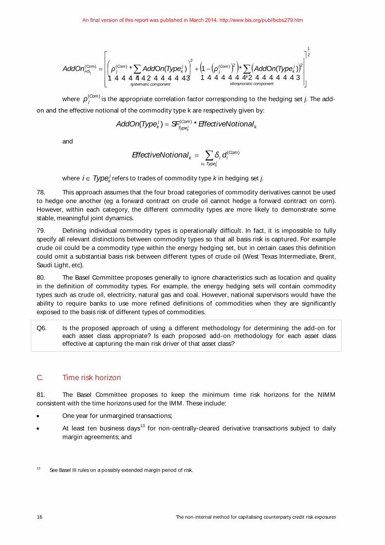
76. The proposed approach for commodity derivatives consists of four hedging sets defined for broad categories of commodity derivatives: energy, metals, agricultural and other commodities. The add-on for the asset class is given by:
∑=j
ComHS
Comj
AddOnAddOn )()(
where the sum is taken over the four hedging sets.
77. Within each hedging set, a single factor model is used to divide the risk of the same type of commodities into a systematic component and an idiosyncratic component, consistent with the approach taken for credit and equity derivatives approaches. Full offsetting/hedging benefits will be allowed between all derivative transactions referencing the same type of commodity, forming a commodity type-level effective notional. Partial offsetting/hedging benefits will be allowed within each hedging set between the same type of commodities (supervisory correlation factors will be defined for each) while no offsetting/hedging benefits will be permitted between hedging sets. In summary, we have:
12 The beta of an individual equity measures the volatility of the stock relative to a broad market index. A value of beta greater
than one means the individual equity is more volatile than the index. The greater the beta is, the more volatile the stock. The beta is calculated by running a linear regression of the stock on the broad index.
An final version of this report was published in March 2014. http://www.bis.org/publ/bcbs279.htm
16 The non-internal method for capitalising counterparty credit risk exposures
( )( ) ( )21
22)(
2)(Com)( )(O*1)(O*
−+
= ∑∑
444444 3444444 2144444 344444 21componentticidiosyncra
k
jk
Comj
componentsystematic
k
jk
ComjHS TypenAddρTypenAddρAddOn
j
where )(Comjρ is the appropriate correlation factor corresponding to the hedging set j. The add-
on and the effective notional of the commodity type k are respectively given by:
kCom
Typej
k otionalEffectiveNSFTypeAddOn jk
*)( )(=
and
∑∈
=j
kTypei
Comiik dδotionalEffectiveN
)(
where jkTypei ∈ refers to trades of commodity type k in hedging set j.
78. This approach assumes that the four broad categories of commodity derivatives cannot be used to hedge one another (eg a forward contract on crude oil cannot hedge a forward contract on corn). However, within each category, the different commodity types are more likely to demonstrate some stable, meaningful joint dynamics.
79. Defining individual commodity types is operationally difficult. In fact, it is impossible to fully specify all relevant distinctions between commodity types so that all basis risk is captured. For example crude oil could be a commodity type within the energy hedging set, but in certain cases this definition could omit a substantial basis risk between different types of crude oil (West Texas Intermediate, Brent, Saudi Light, etc).
80. The Basel Committee proposes generally to ignore characteristics such as location and quality in the definition of commodity types. For example, the energy hedging sets will contain commodity types such as crude oil, electricity, natural gas and coal. However, national supervisors would have the ability to require banks to use more refined definitions of commodities when they are significantly exposed to the basis risk of different types of commodities.
Q6. Is the proposed approach of using a different methodology for determining the add-on for each asset class appropriate? Is each proposed add-on methodology for each asset class effective at capturing the main risk driver of that asset class?
C. Time risk horizon
81. The Basel Committee proposes to keep the minimum time risk horizons for the NIMM consistent with the time horizons used for the IMM. These include:
• One year for unmargined transactions;
• At least ten business days13 for non-centrally-cleared derivative transactions subject to daily margin agreements; and
13 See Basel III rules on a possibly extended margin period of risk.
An final version of this report was published in March 2014. http://www.bis.org/publ/bcbs279.htm
The non-internal method for capitalising counterparty credit risk exposures 17
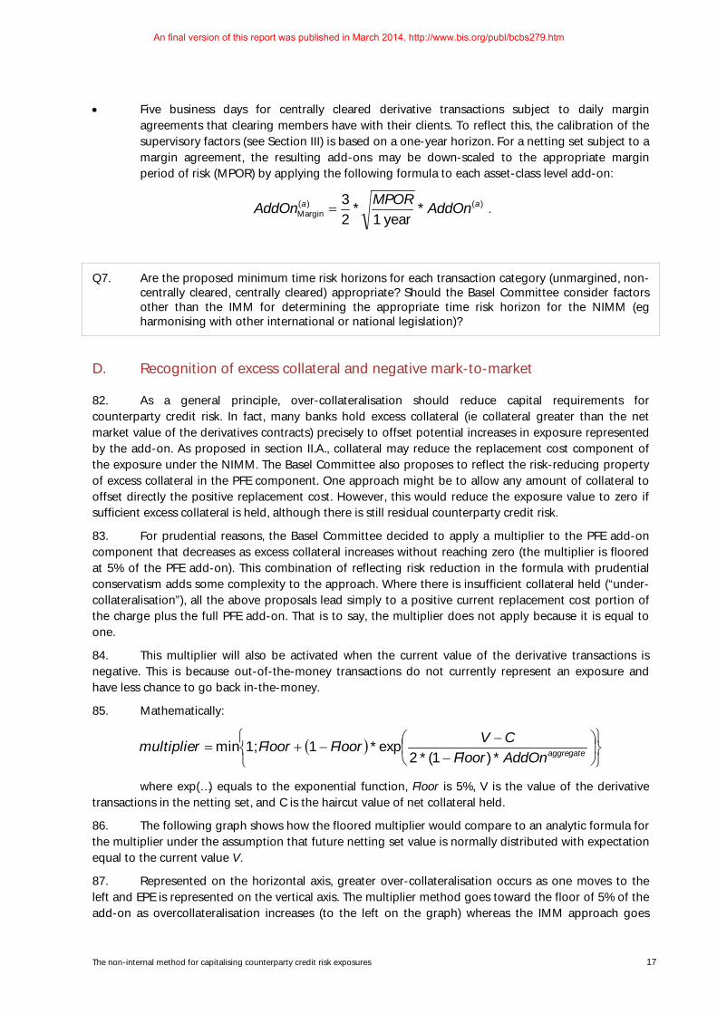
• Five business days for centrally cleared derivative transactions subject to daily margin agreements that clearing members have with their clients. To reflect this, the calibration of the supervisory factors (see Section III) is based on a one-year horizon. For a netting set subject to a margin agreement, the resulting add-ons may be down-scaled to the appropriate margin period of risk (MPOR) by applying the following formula to each asset-class level add-on:
)()(Margin *
year1*
23 aa AddOnMPORAddOn =
.
Q7. Are the proposed minimum time risk horizons for each transaction category (unmargined, non-centrally cleared, centrally cleared) appropriate? Should the Basel Committee consider factors other than the IMM for determining the appropriate time risk horizon for the NIMM (eg harmonising with other international or national legislation)?
D. Recognition of excess collateral and negative mark-to-market
82. As a general principle, over-collateralisation should reduce capital requirements for counterparty credit risk. In fact, many banks hold excess collateral (ie collateral greater than the net market value of the derivatives contracts) precisely to offset potential increases in exposure represented by the add-on. As proposed in section II.A., collateral may reduce the replacement cost component of the exposure under the NIMM. The Basel Committee also proposes to reflect the risk-reducing property of excess collateral in the PFE component. One approach might be to allow any amount of collateral to offset directly the positive replacement cost. However, this would reduce the exposure value to zero if sufficient excess collateral is held, although there is still residual counterparty credit risk.
83. For prudential reasons, the Basel Committee decided to apply a multiplier to the PFE add-on component that decreases as excess collateral increases without reaching zero (the multiplier is floored at 5% of the PFE add-on). This combination of reflecting risk reduction in the formula with prudential conservatism adds some complexity to the approach. Where there is insufficient collateral held (“under-collateralisation”), all the above proposals lead simply to a positive current replacement cost portion of the charge plus the full PFE add-on. That is to say, the multiplier does not apply because it is equal to one.
84. This multiplier will also be activated when the current value of the derivative transactions is negative. This is because out-of-the-money transactions do not currently represent an exposure and have less chance to go back in-the-money.
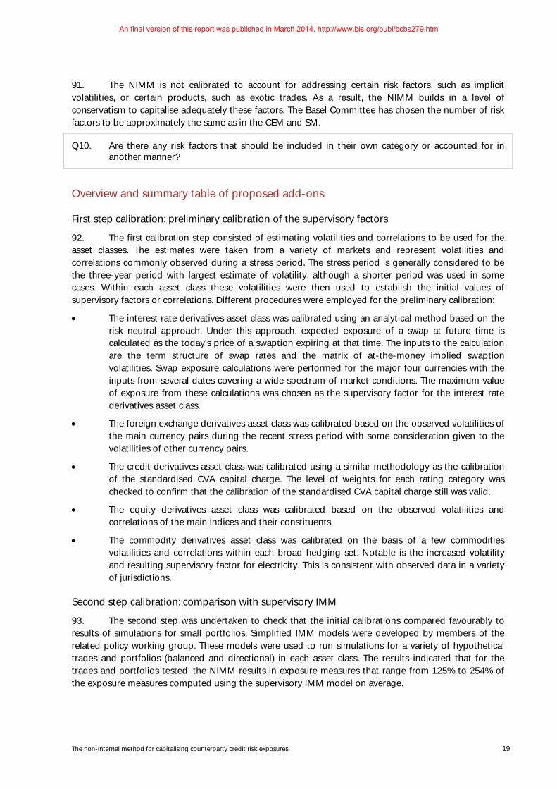
85. Mathematically:
( )
−
−−+= aggregateAddOnFloor
CVFloorFloormultiplier*)1(*2
exp*1;1min
where exp(…) equals to the exponential function, Floor is 5%, V is the value of the derivative transactions in the netting set, and C is the haircut value of net collateral held.
86. The following graph shows how the floored multiplier would compare to an analytic formula for the multiplier under the assumption that future netting set value is normally distributed with expectation equal to the current value V.
87. Represented on the horizontal axis, greater over-collateralisation occurs as one moves to the left and EPE is represented on the vertical axis. The multiplier method goes toward the floor of 5% of the add-on as overcollateralisation increases (to the left on the graph) whereas the IMM approach goes
An final version of this report was published in March 2014. http://www.bis.org/publ/bcbs279.htm

18 The non-internal method for capitalising counterparty credit risk exposures
toward zero. This conservative adjustment does not provide any “cliff effect” and accounts for fat-tailed distributions for changes in exposures.
Q8. Do the suggested formula and 5% floor appropriately recognise the benefits of overcollateralisation?
E. Aggregation across asset classes
88. The Basel Committee proposes not to allow any diversification benefit across asset classes and will therefore simply aggregate the respective add-ons by summation. Mathematically:
∑=a
aaggregate AddOnAddOn )(
where the sum of each asset class is taken.
89. The impact of this assumption in the context of counterparty credit risk exposures has not been fully assessed. The Basel Committee is open to revisiting this treatment based on comments received on the consultative paper and the results of the QIS.
Q9. Is the proposed approach to aggregate across asset classes appropriate?
III. Calibration
90. The NIMM has been calibrated by asset class using a three-step process. First an initial calibration was undertaken to establish the key volatilities and correlations to be used in each asset class. In the second step, the initial calibration was compared to the results of a supervisory CCR model for a variety of portfolios. In the third step, the results of the NIMM were compared to IMM results using some banks’ internal models. The Basel Committee also expects to perform a QIS to assess the impact on banks’ actual portfolios.
An final version of this report was published in March 2014. http://www.bis.org/publ/bcbs279.htm
The non-internal method for capitalising counterparty credit risk exposures 19
91. The NIMM is not calibrated to account for addressing certain risk factors, such as implicit volatilities, or certain products, such as exotic trades. As a result, the NIMM builds in a level of conservatism to capitalise adequately these factors. The Basel Committee has chosen the number of risk factors to be approximately the same as in the CEM and SM.
Q10. Are there any risk factors that should be included in their own category or accounted for in another manner?
Overview and summary table of proposed add-ons
First step calibration: preliminary calibration of the supervisory factors
92. The first calibration step consisted of estimating volatilities and correlations to be used for the asset classes. The estimates were taken from a variety of markets and represent volatilities and correlations commonly observed during a stress period. The stress period is generally considered to be the three-year period with largest estimate of volatility, although a shorter period was used in some cases. Within each asset class these volatilities were then used to establish the initial values of supervisory factors or correlations. Different procedures were employed for the preliminary calibration:
• The interest rate derivatives asset class was calibrated using an analytical method based on the risk neutral approach. Under this approach, expected exposure of a swap at future time is calculated as the today’s price of a swaption expiring at that time. The inputs to the calculation are the term structure of swap rates and the matrix of at-the-money implied swaption volatilities. Swap exposure calculations were performed for the major four currencies with the inputs from several dates covering a wide spectrum of market conditions. The maximum value of exposure from these calculations was chosen as the supervisory factor for the interest rate derivatives asset class.
• The foreign exchange derivatives asset class was calibrated based on the observed volatilities of the main currency pairs during the recent stress period with some consideration given to the volatilities of other currency pairs.
• The credit derivatives asset class was calibrated using a similar methodology as the calibration of the standardised CVA capital charge. The level of weights for each rating category was checked to confirm that the calibration of the standardised CVA capital charge still was valid.
• The equity derivatives asset class was calibrated based on the observed volatilities and correlations of the main indices and their constituents.
• The commodity derivatives asset class was calibrated on the basis of a few commodities volatilities and correlations within each broad hedging set. Notable is the increased volatility and resulting supervisory factor for electricity. This is consistent with observed data in a variety of jurisdictions.
Second step calibration: comparison with supervisory IMM
93. The second step was undertaken to check that the initial calibrations compared favourably to results of simulations for small portfolios. Simplified IMM models were developed by members of the related policy working group. These models were used to run simulations for a variety of hypothetical trades and portfolios (balanced and directional) in each asset class. The results indicated that for the trades and portfolios tested, the NIMM results in exposure measures that range from 125% to 254% of the exposure measures computed using the supervisory IMM model on average.
An final version of this report was published in March 2014. http://www.bis.org/publ/bcbs279.htm
20 The non-internal method for capitalising counterparty credit risk exposures
Third step calibration: IMM benchmarking
94. The third step included a comparison of the NIMM results with banks’ IMM model results for a variety of hypothetical trades and portfolios for each asset class. For these trades and portfolios, IMM benchmark exposures were computed by averaging14 the contributions of a number of participating IMM banks across different jurisdictions. These IMM benchmark exposures were compared to results obtained using NIMM and CEM.
95. The IMM benchmarking was conducted in two separate exercises. The first exercise focused on interest rate derivatives, while the second included a much broader array of asset classes, encompassing additional test portfolios for interest rates, as well as credit, foreign exchange, equities and commodities. A number of trades and portfolios were evaluated, both margined and unmargined, as well as directional and balanced portfolios, stylised hypothetical and portfolios for all five asset classes.
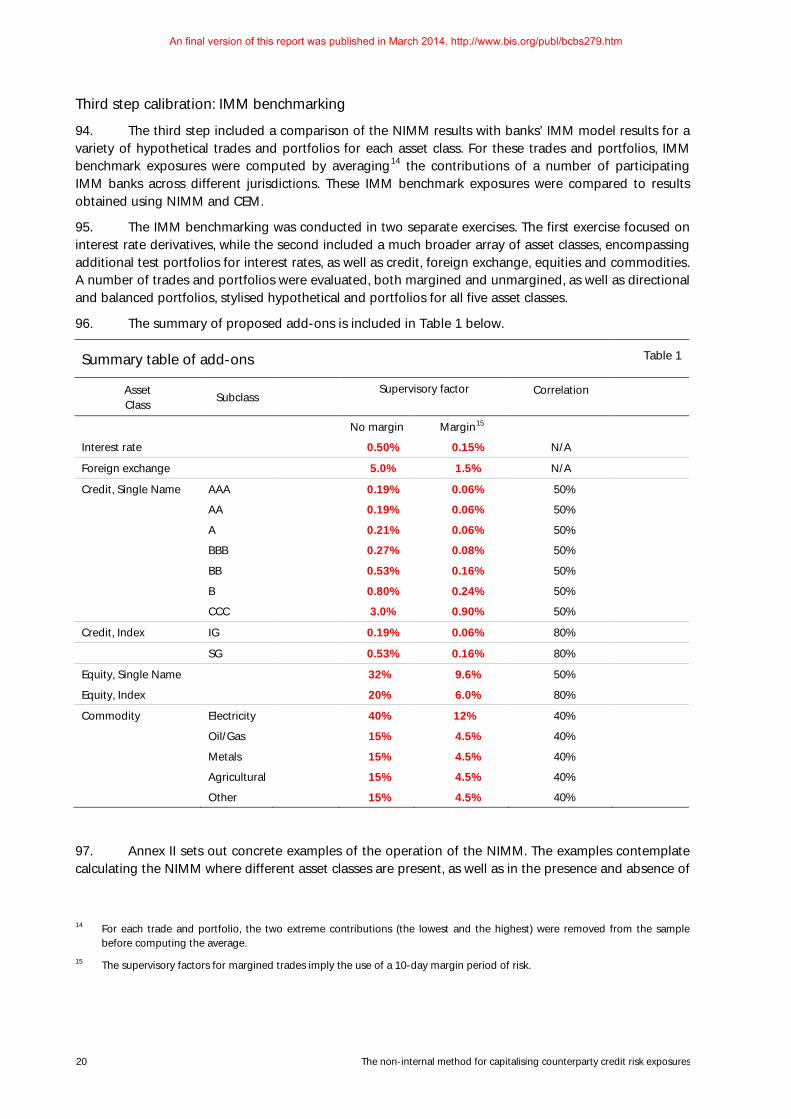
96. The summary of proposed add-ons is included in Table 1 below.
Summary table of add-ons Table 1
Asset Class
Subclass Supervisory factor Correlation
No margin Margin15
Interest rate 0.50% 0.15% N/A
Foreign exchange 5.0% 1.5% N/A
Credit, Single Name AAA 0.19% 0.06% 50%
AA 0.19% 0.06% 50%
A 0.21% 0.06% 50%
BBB 0.27% 0.08% 50%
BB 0.53% 0.16% 50%
B 0.80% 0.24% 50%
CCC 3.0% 0.90% 50%
Credit, Index IG 0.19% 0.06% 80%
SG 0.53% 0.16% 80%
Equity, Single Name 32% 9.6% 50%
Equity, Index 20% 6.0% 80%
Commodity Electricity 40% 12% 40%
Oil/Gas 15% 4.5% 40%
Metals 15% 4.5% 40%
Agricultural 15% 4.5% 40%
Other 15% 4.5% 40%
97. Annex II sets out concrete examples of the operation of the NIMM. The examples contemplate calculating the NIMM where different asset classes are present, as well as in the presence and absence of
14 For each trade and portfolio, the two extreme contributions (the lowest and the highest) were removed from the sample
before computing the average. 15 The supervisory factors for margined trades imply the use of a 10-day margin period of risk.
An final version of this report was published in March 2014. http://www.bis.org/publ/bcbs279.htm
The non-internal method for capitalising counterparty credit risk exposures 21
a margining agreement. Annex III sets out the different steps that need to be taken to calculate the add-ons for interest rate products.
IV. Implication for the IMM shortcut method
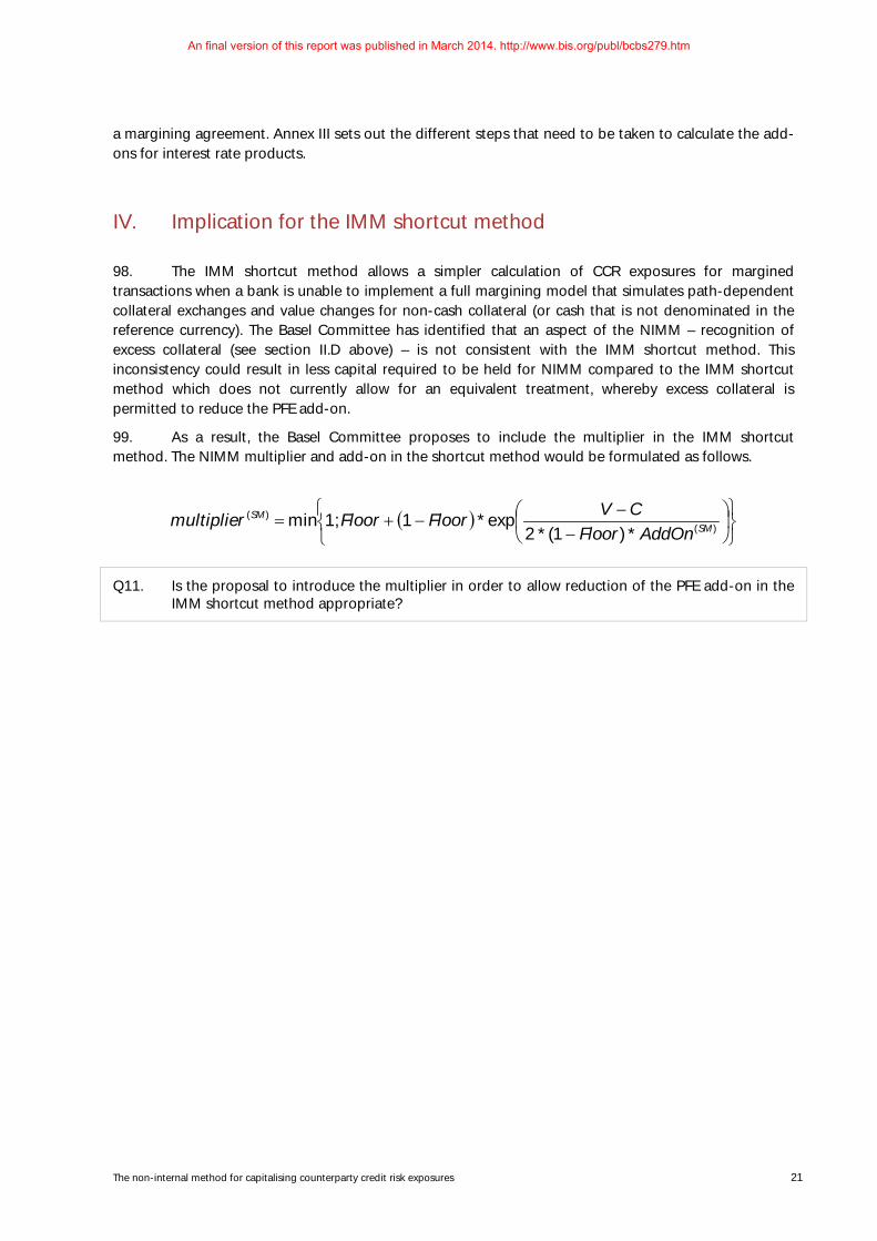
98. The IMM shortcut method allows a simpler calculation of CCR exposures for margined transactions when a bank is unable to implement a full margining model that simulates path-dependent collateral exchanges and value changes for non-cash collateral (or cash that is not denominated in the reference currency). The Basel Committee has identified that an aspect of the NIMM – recognition of excess collateral (see section II.D above) – is not consistent with the IMM shortcut method. This inconsistency could result in less capital required to be held for NIMM compared to the IMM shortcut method which does not currently allow for an equivalent treatment, whereby excess collateral is permitted to reduce the PFE add-on.
99. As a result, the Basel Committee proposes to include the multiplier in the IMM shortcut method. The NIMM multiplier and add-on in the shortcut method would be formulated as follows.
( )
−
−−+= )(
)(
*)1(*2exp*1;1min SM
SM
AddOnFloorCVFloorFloormultiplier
Q11. Is the proposal to introduce the multiplier in order to allow reduction of the PFE add-on in the IMM shortcut method appropriate?
An final version of this report was published in March 2014. http://www.bis.org/publ/bcbs279.htm

22 The non-internal method for capitalising counterparty credit risk exposures
Annex I
Glossary of terms
1. Current replacement cost
Current exposure is the larger of zero, or the market value of a transaction or portfolio of transactions within a netting set with a counterparty that would be lost upon the default of the counterparty, assuming no recovery on the value of those transactions in bankruptcy. Current replacement cost is often also called replacement cost.
2. Future exposure
Estimation of the current exposure at any particular future date. Future exposure is usually expressed in terms of the average of future values at a given time (expected exposure) or as a percentile of future values at a given time (potential future exposure).
3. Risk position
Risk number that is assigned to a transaction under the CCR standardised method using the regulatory algorithm.
4. Delta-equivalent notional value
Measure of the risk position for a non-linear OTC derivative transaction under the CCR standardised method based on an equivalent amount in the underlying main risk factor derived from the sensitivity of this risk factor to the derivative value.
5. Independent collateral amount (ICA)
Represents collateral posted by the counterparty that the bank may seize upon default of the counterparty, the amount of which does not change in response to the value of the transactions it secures plus Independent Amount in the ISDA terminology.
6. Margin period of risk
The time period from the last exchange of collateral covering a netting set of transactions with a defaulting counterpart until that counterpart is closed out and the resulting market risk is re-hedged.
7. Margined transactions
Transactions subject to certain margin agreements where counterparties commit to exchange collateral due to future changes in the market value of derivative transactions to offset any future imbalances.
An final version of this report was published in March 2014. http://www.bis.org/publ/bcbs279.htm
The non-internal method for capitalising counterparty credit risk exposures 23
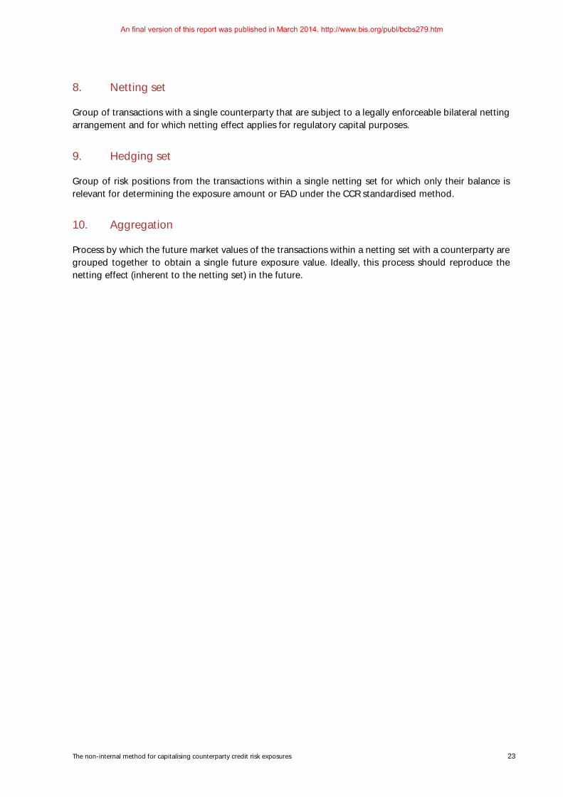
8. Netting set
Group of transactions with a single counterparty that are subject to a legally enforceable bilateral netting arrangement and for which netting effect applies for regulatory capital purposes.
9. Hedging set
Group of risk positions from the transactions within a single netting set for which only their balance is relevant for determining the exposure amount or EAD under the CCR standardised method.
10. Aggregation
Process by which the future market values of the transactions within a netting set with a counterparty are grouped together to obtain a single future exposure value. Ideally, this process should reproduce the netting effect (inherent to the netting set) in the future.
An final version of this report was published in March 2014. http://www.bis.org/publ/bcbs279.htm

24 The non-internal method for capitalising counterparty credit risk exposures
Annex II
Application of the NIMM to sample portfolios
Example 1
Netting set 1 consists of three interest rates derivatives: two fixed vs floating IRS and one purchased European swaption. The table below summarises the relevant contractual terms of the three derivatives.
(*) For the swaption, the legs are those of the underlying swap.
All notional amounts and market values in the table are given in USD.
The netting set is not subject to a margin agreement and there is no exchange of collateral (independent amount/initial margin) at inception. According to the NIMM formula, the EAD for unmargined netting set is given by:
)*(* aggregateAddOnmultiplierRCalphaEAD +=
The replacement cost is calculated at netting set level as a simple algebraic sum (floored at zero) of the derivatives’ market values at the reference date. Thus, using the market values indicated in the table (expressed in thousand):
( ) ( ) 600 ;502030max0 ;max =+−=−= CVRC
Since V-C is positive (equal to V, 60,000), the value of the multiplier is 1, as explained in the consultative paper. The PFE add-on is first calculated at hedging set level and then aggregated across hedging sets inside the netting set. In this example, regardless of the method chosen for treating the maturity mismatch, the netting set is made of two hedging sets, since the trades refer to interest rates denominated in two different currencies (USD and EUR) and each trade belongs to the third maturity bucket (>5 years):
{ }2 ,1 1 tradetradeHS =
{ }3 2 tradeHS =
For each IR trade, the adjusted notional is calculated according to:
( )1 ;max* )(ii
IRi SENotionalTraded −=
where iS and iE are defined as follows:
• Ongoing linear transactions: 0=iS and iE is the latest date when a cash flow is possible
Trade #
Nature Residual maturity
Base currency
Notional (thousand)
Pay Leg (*)
Receive Leg (*)
Market value
(thousand)
1 Interest rate swap 10 years USD 10,000 Fixed Floating 30
2 Interest rate swap 6 years USD 10,000 Floating Fixed -20
3 European swaption 1x10 years EUR 5,000 Floating Fixed 50
An final version of this report was published in March 2014. http://www.bis.org/publ/bcbs279.htm
The non-internal method for capitalising counterparty credit risk exposures 25
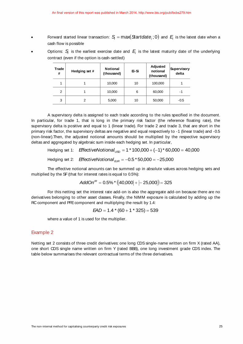
• Forward started linear transaction: ( )0 ;max ii StartdateS = and iE is the latest date when a cash flow is possible
• Options: iS is the earliest exercise date and iE is the latest maturity date of the underlying contract (even if the option is cash-settled)
A supervisory delta is assigned to each trade according to the rules specified in the document. In particular, for trade 1, that is long in the primary risk factor (the reference floating rate), the supervisory delta is positive and equal to 1 (linear trade). For trade 2 and trade 3, that are short in the primary risk factor, the supervisory deltas are negative and equal respectively to -1 (linear trade) and -0.5 (non-linear).Then, the adjusted notional amounts should be multiplied by the respective supervisory deltas and aggregated by algebraic sum inside each hedging set. In particular,
Hedging set 1: 000,40000,60*)1(000,100*1USD =−+=otionalEffectiveN
Hedging set 2: 000,25000,50*5.0 −=−=EURotionalEffectiveN
The effective notional amounts can be summed up in absolute values across hedging sets and multiplied by the SF (that for interest rates is equal to 0.5%):
( ) 325000,25000,40*%5.0 =−+=IRAddOn
For this netting set the interest rate add-on is also the aggregate add-on because there are no derivatives belonging to other asset classes. Finally, the NIMM exposure is calculated by adding up the RC component and PFE component and multiplying the result by 1.4:
539)325*160(*4.1 =+=EAD
where a value of 1 is used for the multiplier.
Example 2
Netting set 2 consists of three credit derivatives: one long CDS single-name written on firm X (rated AA), one short CDS single name written on firm Y (rated BBB), one long investment grade CDS index. The table below summarises the relevant contractual terms of the three derivatives.
Trade #
Hedging set # Notional
(thousand) Ei-Si
Adjusted notional
(thousand)
Supervisory delta
1 1 10,000 10 100,000 1
2 1 10,000 6 60,000 -1
3 2 5,000 10 50,000 -0.5
An final version of this report was published in March 2014. http://www.bis.org/publ/bcbs279.htm
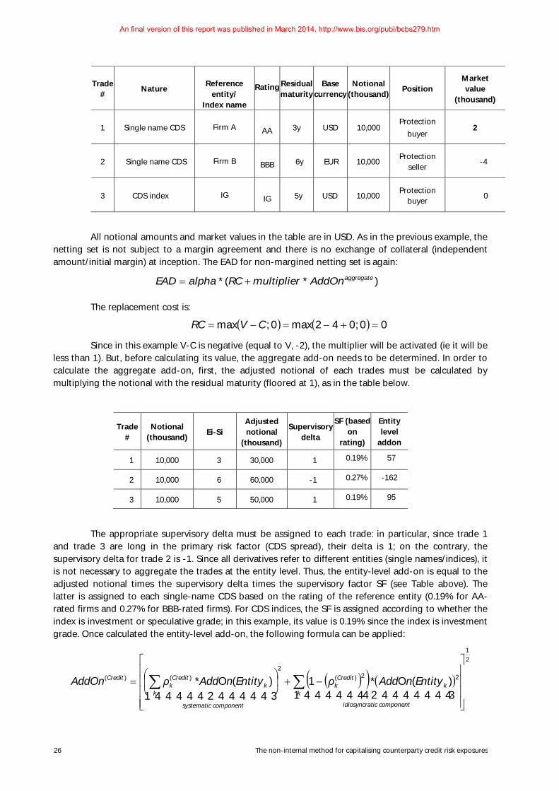
26 The non-internal method for capitalising counterparty credit risk exposures
All notional amounts and market values in the table are in USD. As in the previous example, the netting set is not subject to a margin agreement and there is no exchange of collateral (independent amount/initial margin) at inception. The EAD for non-margined netting set is again:
)*(* aggregateAddOnmultiplierRCalphaEAD +=
The replacement cost is:
( ) ( ) 00 ;042max0 ;max =+−=−= CVRC
Since in this example V-C is negative (equal to V, -2), the multiplier will be activated (ie it will be less than 1). But, before calculating its value, the aggregate add-on needs to be determined. In order to calculate the aggregate add-on, first, the adjusted notional of each trades must be calculated by multiplying the notional with the residual maturity (floored at 1), as in the table below.
The appropriate supervisory delta must be assigned to each trade: in particular, since trade 1 and trade 3 are long in the primary risk factor (CDS spread), their delta is 1; on the contrary, the supervisory delta for trade 2 is -1. Since all derivatives refer to different entities (single names/indices), it is not necessary to aggregate the trades at the entity level. Thus, the entity-level add-on is equal to the adjusted notional times the supervisory delta times the supervisory factor SF (see Table above). The latter is assigned to each single-name CDS based on the rating of the reference entity (0.19% for AA-rated firms and 0.27% for BBB-rated firms). For CDS indices, the SF is assigned according to whether the index is investment or speculative grade; in this example, its value is 0.19% since the index is investment grade. Once calculated the entity-level add-on, the following formula can be applied:
( )( ) ( )
21
22)(
2)()( )(O*1)(O*
−+
= ∑∑
4444444 34444444 2144444 344444 21componentticidiosyncra
kk
Creditk
componentsystematic
kk
Creditk
Credit EntitynAddρEntitynAddρAddOn
Trade #
Nature
Reference
entity/ Index name
Rating Residual
maturity Base
currency Notional
(thousand) Position
Market value
(thousand)
1 Single name CDS
Firm A
AA 3y USD 10,000 Protection
buyer 2
2 Single name CDS
Firm B
BBB 6y EUR 10,000 Protection
seller -4
3 CDS index
IG
IG 5y USD 10,000 Protection
buyer 0
Trade #
Notional (thousand) Ei-Si
Adjusted notional
(thousand)
Supervisory delta
SF (based on
rating)
Entity level
addon
1 10,000 3 30,000 1 0.19% 57
2 10,000 6 60,000 -1 0.27% -162
3 10,000 5 50,000 1 0.19% 95
An final version of this report was published in March 2014. http://www.bis.org/publ/bcbs279.htm
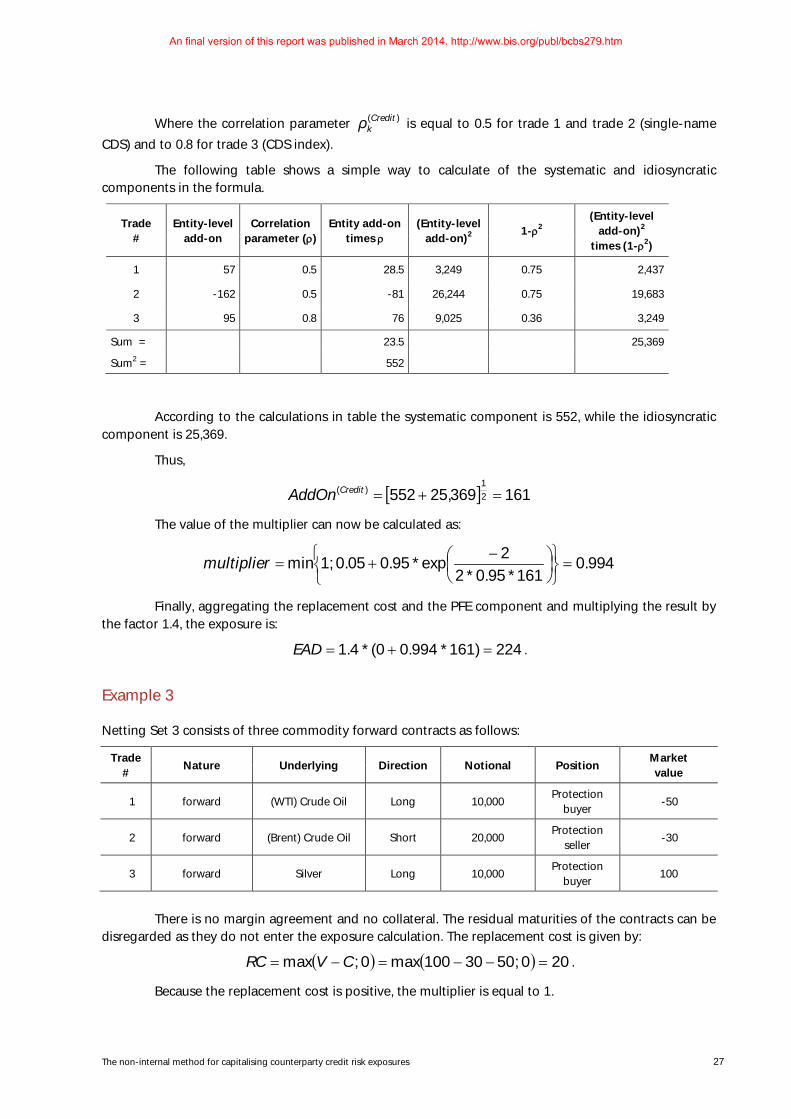
The non-internal method for capitalising counterparty credit risk exposures 27
Where the correlation parameter )(Creditkρ is equal to 0.5 for trade 1 and trade 2 (single-name
CDS) and to 0.8 for trade 3 (CDS index).
The following table shows a simple way to calculate of the systematic and idiosyncratic components in the formula.
According to the calculations in table the systematic component is 552, while the idiosyncratic component is 25,369.
Thus,
[ ] 161369,25552 21
)( =+=CreditAddOn
The value of the multiplier can now be calculated as:
994.0161*95.0*2
2exp*95.005.0 ;1min =
−
+=multiplier
Finally, aggregating the replacement cost and the PFE component and multiplying the result by the factor 1.4, the exposure is:
224)161*994.00(*4.1 =+=EAD .
Example 3
Netting Set 3 consists of three commodity forward contracts as follows:
Trade # Nature Underlying Direction Notional Position
Market value
1 forward (WTI) Crude Oil Long 10,000 Protection
buyer -50
2 forward (Brent) Crude Oil Short 20,000 Protection
seller -30
3 forward Silver Long 10,000 Protection
buyer 100
There is no margin agreement and no collateral. The residual maturities of the contracts can be
disregarded as they do not enter the exposure calculation. The replacement cost is given by:
( ) ( ) 200 ;5030100max0 ;max =−−=−= CVRC .
Because the replacement cost is positive, the multiplier is equal to 1.
Trade #
Entity-level add-on
Correlation parameter (ρ)
Entity add-on times ρ
(Entity-level add-on)2
1-ρ2 (Entity-level
add-on)2 times (1-ρ2)
1 57 0.5 28.5 3,249 0.75 2,437
2 -162 0.5 -81 26,244 0.75 19,683
3 95 0.8 76 9,025 0.36 3,249
Sum = 23.5 25,369
Sum2 = 552
An final version of this report was published in March 2014. http://www.bis.org/publ/bcbs279.htm
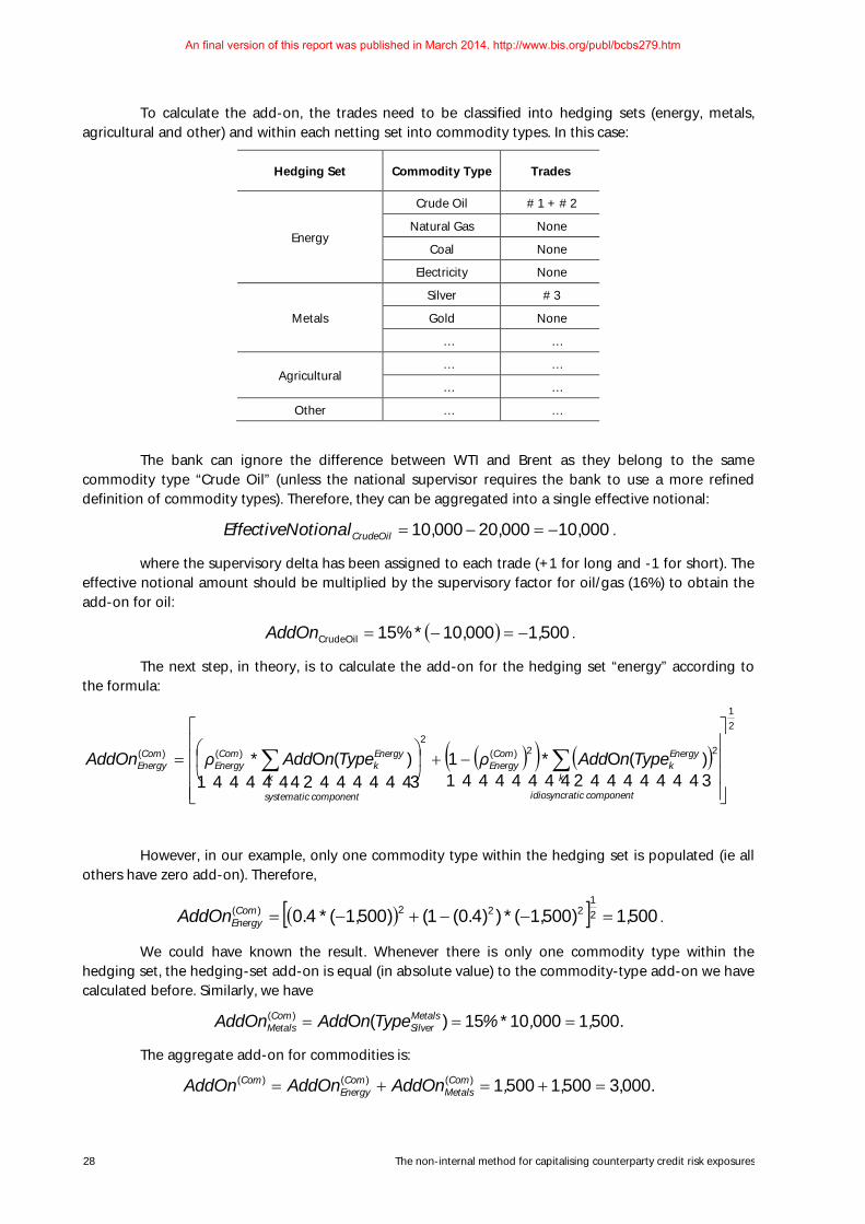
28 The non-internal method for capitalising counterparty credit risk exposures
To calculate the add-on, the trades need to be classified into hedging sets (energy, metals, agricultural and other) and within each netting set into commodity types. In this case:
Hedging Set Commodity Type Trades
Energy
Crude Oil # 1 + # 2
Natural Gas None
Coal None
Electricity None
Metals
Silver # 3
Gold None
… …
Agricultural … …
… …
Other … …
The bank can ignore the difference between WTI and Brent as they belong to the same commodity type “Crude Oil” (unless the national supervisor requires the bank to use a more refined definition of commodity types). Therefore, they can be aggregated into a single effective notional:
000,10000,20000,10 −=−=CrudeOilotionalEffectiveN .
where the supervisory delta has been assigned to each trade (+1 for long and -1 for short). The effective notional amount should be multiplied by the supervisory factor for oil/gas (16%) to obtain the add-on for oil:
( ) 5001000,10*%15CrudeOil ,AddOn −=−= .
The next step, in theory, is to calculate the add-on for the hedging set “energy” according to the formula:
( )( ) ( )21
22)(
2)()( )(O*1)(O*
−+
= ∑∑
4444444 34444444 21444444 3444444 21componentticidiosyncra
k
Energyk
ComEnergy
componentsystematic
k
Energyk
ComEnergy
ComEnergy TypenAddρTypenAddρAddOn
However, in our example, only one commodity type within the hedging set is populated (ie all others have zero add-on). Therefore,
( )[ ] 500,1)500,1(*))4.0(1()500,1(*4.0 21
222)( =−−+−=ComEnergyAddOn .
We could have known the result. Whenever there is only one commodity type within the hedging set, the hedging-set add-on is equal (in absolute value) to the commodity-type add-on we have calculated before. Similarly, we have
.500100010*15)(O)( ,,%TypenAddAddOn MetalsSilver
ComMetals ===
The aggregate add-on for commodities is:
.000,3500,15001)()()( =+=+= ,AddOnAddOnAddOn ComMetals
ComEnergy
Com
An final version of this report was published in March 2014. http://www.bis.org/publ/bcbs279.htm
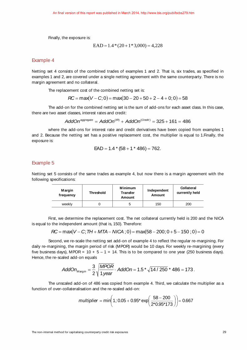
The non-internal method for capitalising counterparty credit risk exposures 29
Finally, the exposure is:
228,4)000,3*120(*4.1EAD =+=
Example 4
Netting set 4 consists of the combined trades of examples 1 and 2. That is, six trades, as specified in examples 1 and 2, are covered under a single netting agreement with the same counterparty. There is no margin agreement and no collateral.
The replacement cost of the combined netting set is:
( ) ( ) 580 ;042502030max0 ;max =+−++−=−= CVRC
The add-on for the combined netting set is the sum of add-ons for each asset class. In this case, there are two asset classes, interest rates and credit:
486161325)()( =+=+= CreditIRaggregate AddOnAddOnAddOn
where the add-ons for interest rate and credit derivatives have been copied from examples 1 and 2. Because the netting set has a positive replacement cost, the multiplier is equal to 1.Finally, the exposure is:
.762)486*158(*4.1EAD =+=
Example 5
Netting set 5 consists of the same trades as example 4, but now there is a margin agreement with the following specifications:
Margin frequency
Threshold Minimum Transfer Amount
Independent Amount
Collateral currently held
weekly 0 5 150 200
First, we determine the replacement cost. The net collateral currently held is 200 and the NICA is equal to the independent amount (that is, 150). Therefore:
( ) ( ) 00 ; 15050 ;20058max0 ; ;max =−+−=−+−= NICAMTATHCVRC
Second, we re-scale the netting set add-on of example 4 to reflect the regular re-margining. For daily re-margining, the margin period of risk (MPOR) would be 10 days. For weekly re-margining (every five business days), MPOR = 10 + 5 – 1 = 14. This is to be compared to one year (250 business days). Hence, the re-scaled add-on equals
173486*250/14*5.112
3arg ==⋅= AddOn
yearMPORAddOn inM .
The unscaled add-on of 486 was copied from example 4. Third, we calculate the multiplier as a function of over-collateralisation and the re-scaled add-on:
66701739502
20058exp950050 1min .*.*
*..;multiplier =
−
+=
An final version of this report was published in March 2014. http://www.bis.org/publ/bcbs279.htm

30 The non-internal method for capitalising counterparty credit risk exposures
Finally, the exposure is:
1621736670041 =+= )*.*(.EAD
Example 6
Netting set 6 is identical to netting set 1, except for the maturity of derivative 2, which in this case is four years. The table below summarises the contractual features of the three derivatives. All notional amounts and market values in the table are given in USD.
Trade #
Nature Residual maturity
Base currency
Notional (thousand)
Pay Leg (*)
Receive Leg (*)
Market value
(thousand) 1 Interest rate swap 10 years USD 10,000 Fixed Floating 30
2 Interest rate swap 4 years USD 10,000 Floating Fixed -20
3 European swaption 1x10 years EUR 5,000 Floating Fixed 50
The netting set is not subject to a margin agreement and there is no exchange of collateral (independent amount/initial margin) at inception.
As in example 1, the replacement cost is 60 and the value of the multiplier is 1. Differently from example 1, the add-on calculation implies the necessity to deal with maturity mismatch inside the USD currency, in consideration of the three maturity buckets proposed in the consultative paper (less than one year, between one and five years and more than five years). The calculation can be done according to one of the two approaches outlined in the consultative paper.
Approach 1: Partial recognition of offsetting between 3 maturity buckets
According to this approach, aggregation of adjusted notionals across time buckets inside the same hedging set is performed on the basis of the following formula:
( ) ( ) ( )[ ] 21
)(3
)(1
)(3
)(2
)(2
)(1
2)(3
2)(2
2)(1
)( **6.0**4.1**4.1 IRj
IRj
IRj
IRj
IRj
IRj
IRj
IRj
IRj
IRj DDDDDDDDDotionalEffectiveN +++++=
Thus, using the supervisory deltas and adjusted notionals of trade 1 and trade 2 calculated in example 1 (modified to take into account the different residual maturity of trade 2), the effective notional amount for the USD hedging set is given by:
[ ] 460,77 000,100*)000,40(*4.1000,100000,40 21
22)( =−++=IRUSDotionalEffectiveN
As in example 1, the effective notional amount for the EUR hedging set is -25,000. Summing up the effective notional amounts in absolute value across currencies and multiplying the result by the interest rate SF (0.5%) we get:
( ) 512000,25460,77*%5.0)( =−+=IRAddOn
Finally, the exposure is the sum of the RC component and PFE component multiplied by 1.4:
801)512*160(*4.1 =+=EAD
Approach 2: No recognition of offsetting between 3 maturity buckets
As explained in the consultative paper, approach 2 does not recognise any offset across time buckets. Applying the formula for the USD hedging set, we get:
An final version of this report was published in March 2014. http://www.bis.org/publ/bcbs279.htm

The non-internal method for capitalising counterparty credit risk exposures 31
000,140000,100000,40)( =+−=IRUSDotionalEffectiveN
Since the effective notional amount for the EUR hedging set is still -25,000, the interest rate add-on is
( ) 825000,25000,140*%5.0 =−+=IRAddOn
And the exposure is:
1239)825*160(*4.1 =+=EAD
An final version of this report was published in March 2014. http://www.bis.org/publ/bcbs279.htm
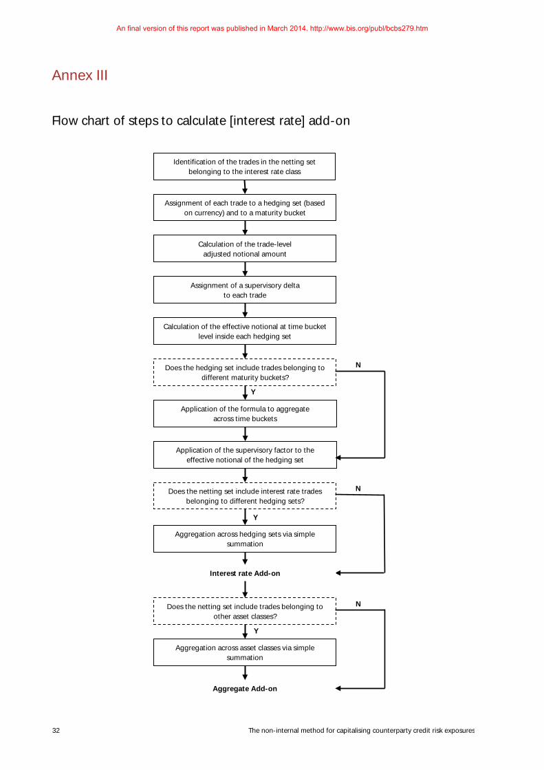
32 The non-internal method for capitalising counterparty credit risk exposures
Annex III
Flow chart of steps to calculate [interest rate] add-on
Y
Y
N
Y
Identification of the trades in the netting set belonging to the interest rate class
Calculation of the trade-level adjusted notional amount
Assignment of a supervisory delta to each trade
Calculation of the effective notional at time bucket level inside each hedging set
Application of the formula to aggregate across time buckets
Does the hedging set include trades belonging to different maturity buckets?
Does the netting set include interest rate trades belonging to different hedging sets?
Aggregation across hedging sets via simple summation
Application of the supervisory factor to the effective notional of the hedging set
Assignment of each trade to a hedging set (based on currency) and to a maturity bucket
N
Interest rate Add-on
Does the netting set include trades belonging to other asset classes?
Aggregation across asset classes via simple summation
Aggregate Add-on
N
An final version of this report was published in March 2014. http://www.bis.org/publ/bcbs279.htm