Embed Size (px)
Citation preview

NewsThe Newsletter of the R Project Volume 6/5, December 2006
Editorialby Wolfgang Huber and Paul Murrell
Welcome to the fifth and final issue of R News for2006, our third special issue of the year, with a fo-cus on the use of R in Bioinformatics. Many thanksto guest editor Wolfgang Huber for doing a fantasticjob in putting this issue together.
Paul MurrellThe University of Auckland, New [email protected]
Biology is going through a revolution. Thegenome sequencing projects that were initiated in the1980’s and undertaken in the 1990’s have providedfor the first time systematic inventories of the com-ponents of biological systems. Technological innova-tion is producing ever more detailed measurementson the functioning of these components and their in-teractions. The Internet has opened possibilities forthe sharing of data and of computational resourcesthat would have been unimaginable only 15 yearsago.
The field of bioinformatics emerged in the 1990’sto deal with the pressing questions that the mas-sive amounts of new sequence data posed: sequence
alignment, similarity and clustering, their phyloge-netic interpretation, genome assembly, sequence an-notation, protein structure. C and Perl were the lan-guages of choice for the first generation of bioinfor-maticians. All of these question remain relevant, yetin addition we now have the big and colourful fieldof functional genomics, which employs all sorts oftechnologies to measure the abundances and activi-ties of biomolecules under different conditions, maptheir interactions, monitor the effect of their pertur-bation on the phenotype of a cell or even a wholeorganism, and eventually to build predictive modelsof biological systems.
R is well suited to many of the scientific and com-putational challenges in functional genomics. Someof the efforts in this field have been pulled togethersince 2001 by the Bioconductor project, and many ofthe papers in this issue report on packages from theproject. But Bioconductor is more than just a CRAN-style repository of biology-related packages. Moti-vated by the particular challenges of genomic data,the project has actively driven a number of tech-nological innovations that have flown back into R,among these, package vignettes, an embracementof S4, the management of extensive package de-pendence hierarchies, and interfaces between R and
Contents of this issue:
Editorial . . . . . . . . . . . . . . . . . . . . . . 1Graphs and Networks: Tools in Bioconductor . 2Modeling Package Dependencies Using Graphs 8Image Analysis for Microscopy Screens . . . . 12beadarray: An R Package to Analyse Illumina
BeadArrays . . . . . . . . . . . . . . . . . . . 17Transcript Mapping with High-Density Tiling
Arrays . . . . . . . . . . . . . . . . . . . . . . 23Analyzing Flow Cytometry Data with Biocon-
ductor . . . . . . . . . . . . . . . . . . . . . . 27Protein Complex Membership Estimation us-
ing apComplex . . . . . . . . . . . . . . . . . 32
SNP Metadata Access and Use with Biocon-ductor . . . . . . . . . . . . . . . . . . . . . . 36
Integrating Biological Data Resources into Rwith biomaRt . . . . . . . . . . . . . . . . . . 40
Identifying Interesting Genes with siggenes . 45Reverse Engineering Genetic Networks using
the GeneNet Package . . . . . . . . . . . . . . 50A Multivariate Approach to Integrating
Datasets using made4 and ade4 . . . . . . . . 54Using amap and ctc Packages for Huge Clus-
tering . . . . . . . . . . . . . . . . . . . . . . . 58Model-based Microarray Image Analysis . . . 60Sample Size Estimation for Microarray Exper-
iments Using the ssize Package . . . . . . . . 64

Vol. 6/5, December 2006 2
other software systems. Biological metadata (for ex-ample, genome annotations) need to be tightly inte-grated with the analysis of primary data, and the Bio-conductor project has invested a lot of effort in theprovision of high quality metadata packages. The ex-perimental data in functional genomics require morestructured formats than the basic data types of R, andone of the main products of the Bioconductor core isthe provision of common data structures that allowthe efficient exchange of data and computational re-sults between different packages. One example is theExpressionSet, an S4 class for the storage of the es-sential data and information on a microarray experi-ment.
The articles in this issue span a wide range of top-ics. Common themes are preprocessing (data import,
quality assessment, standardization, error modelingand summarization), pattern discovery and detection,and higher level statistical models with which weaim to gain insight into the underlying biologicalprocesses. Sometimes, the questions that we en-counter in bioinformatics result in methods that havepotentially a wider applicability; this is true in par-ticular for the first three articles with which we startthis issue.
Wolfgang HuberEuropean Bioinformatics Insitute (EBI)European Molecular Biology Laboratory (EMBL) Cam-bridge, [email protected]
Graphs and Networks: Tools inBioconductorby Li Long and Vince Carey
Introduction
Network structures are fundamental components forscientific modeling in a number of substantive do-mains, including sociology, ecology, and computa-tional biology. The mathematical theory of graphscomes immediately into play when the entities andprocesses being modeled are clearly organized intoobjects (modeled as graph nodes) and relationships(modeled as graph edges).
Graph theory addresses the taxonomy of graphstructures, the measurement of general features ofconnectedness, complexity of traversals, and manyother combinatorial and algebraic concepts. An im-portant generalization of the basic concept of graph(traditionally defined as a set of nodes N and a bi-nary relation E on N defining edges) is the hyper-graph (in which edges are general subsets of thenode set of cardinality at least 2).
The basic architecture of the Bioconductor toolkitfor graphs and networks has the following structure:
• Representation infrastructure: packages graph,hypergraph;
• Algorithms for traversal and measurement:packages RBGL, graphPart
• Algorithms for layout and visualization: pack-age Rgraphviz; RBGL also includes some lay-out algorithms;
• Packages for addressing substantive prob-lems in bioinformatics: packages pathRender,
GraphAT, ScISI, GOstats, ontoTools, and oth-ers.
In this article we survey aspects of working withnetwork structures with some of these Bioconductortools.
The basics: package graph
The graph package provides a variety of S4 classesrepresenting graphs. A virtual class graph definesthe basic structure:
> library(graph)> getClass("graph")Virtual Class
Slots:
Name: edgemode edgeData nodeDataClass: character attrData attrData
Known Subclasses: "graphNEL", "graphAM","graphH", "distGraph", "clusterGraph","generalGraph"
A widely used concrete extension of this class isgraphNEL, denoting the “node and edge list” repre-sentation:
> getClass("graphNEL")
Slots:
Name: nodes edgeL edgemode edgeDataClass: vector list character attrData
R News ISSN 1609-3631

Vol. 6/5, December 2006 3
attrDatanodeData
Extends: "graph"
An example graph is supplied, representing the“integrin mediated cell adhesion” pathway as de-fined in a previous version of KEGG (Kyoto Ency-clopedia of Genes and Genomes, Kanehisa and Goto,2000; the pathway is now called “focal adhesion”).
> data(integrinMediatedCellAdhesion)> IMCAGraphA graphNEL graph with directed edgesNumber of Nodes = 52Number of Edges = 91> nodes(IMCAGraph)[1:5][1] "ITGB" "ITGA" "ILK" "CAV" "SHC"> edges(IMCAGraph)[1:5]$ITGB[1] "ITGA" "ILK" "CAV" "SHC" "ACTN" "TLN"
$ITGA[1] "ITGB"
$ILK[1] "ITGB"
$CAV[1] "ITGB"
$SHC[1] "FYN" "GRB2" "ITGB"
Methods that can be used to work with graph in-stances include:
• The edgemode method returns a character to-ken indicating whether the graph is directed orundirected.
• The nodes method returns information ongraph nodes; in the case of a graphNEL in-stance it returns a vector, intended to repre-sent the (unordered) node set through charac-ter names of entities described by the graph.(Note that there are more general represen-tations available, in which objects other thanstrings can constitute graph nodes, see remarkson nodeData below.)
• The edges method returns a named list. The ithelement of the list bears as its name the nameof the ith node, and contains a vector of nodenames to which the ith node is directly linkedby a graph edge.
> all.equal(names(edges(IMCAGraph)),nodes(IMCAGraph))
[1] TRUE
The network may be visualized using the follow-ing code:
library(Rgraphviz)plot(IMCAGraph,
attrs = IMCAAttrs$defAttrs,nodeAttrs = IMCAAttrs$nodeAttrs,subGList = IMCAAttrs$subGList);
See Figure 1.
Figure 1: Rendering of the IMCA pathway.
We will illustrate aspects of other parts of the sys-tem using this example graph structure.
The Rgraphviz package
Rgraphviz provides an interface to graphviz1,an open source library for graph visualization.Graphviz performs several types of graph layout:
• dot: draws directed graphs in a hierarchicalway
• neato: draws graphs using Kamada-Kawai al-gorithm
• fdp: draws graphs using Fruchterman-Reingold heuristic
• twopi: draws radial layout• circo: draws circular layout
Many aspects of graph rendering are covered,with general programmatic control over colors,fonts, shapes, and line styles employed for variousaspects of the display and annotation of the graph.
The Bioconductor Rgraphviz interface packagelets you choose the layout engine for your graph ob-ject among the options dot (the default), neato andtwopi.
1http://www.graphviz.org
R News ISSN 1609-3631

Vol. 6/5, December 2006 4
We generate a graph and plot it using differentlayout engines:
> library("Rgraphviz")> set.seed(123)> V <- letters[1:10]> M <- 1:4> g1 <- randomGraph(V, M, 0.2)A graphNEL graph with undirected edgesNumber of Nodes = 10Number of Edges = 16
> plot(g1)
a
b
c
d
e
f
g
h
i j
Figure 2: Rendering with dot.
> plot(g1, "neato")
a b
c
d ef
gh
i
j
Figure 3: Rendering with neato.
> plot(g1, "twopi")
a
b
c
d
e
f
gh i
j
Figure 4: Rendering with twopi.
The RBGL package
Researchers study different kinds of biological net-works: protein interaction networks, genetic regu-latory systems, metabolic networks are a few exam-ples. Signaling pathway identification could be mod-eled using shortest paths in a protein interaction net-work. The task of identification of protein complexescan be conducted by finding cohesive subgroups inprotein interaction networks. The protein interactionnetwork under consideration is built from the experi-mental data, which contains incomplete information,false positives and false negatives. Extensible repre-sentations that can manage such complications are ata premium in this process.
RBGL provides a set of graph algorithms to anal-yse the structures and properties of graphs and net-works.
There are three categories of algorithms in thispackage:
• interfaces to graph algorithms from the boost2
graph library (BGL3);
• algorithms built on BGL; and
• other algorithms.
The Boost C++ Library provides peer-reviewedC++ libraries, with the objective of creating highlyportable open source resources for C++ program-ming analogous to the proprietary standard templatelibrary (STL).
The Boost Graph Library (BGL) is one of the Boostlibraries. BGL provides a set of generic data struc-tures to represent graphs, and a collection of C++modules (all defined as templates) constituting algo-rithms on graphs.
Package RBGL provides a direct interface tomany of the graph algorithms available in BGL. Table1 lists the main functionalities currently provided.
In the second category, we implementedminimum-cut algorithm minCut, based on one ofthe maximum-flow algorithms from BGL.
In the third category, we implemented
• highly connected subgraphs (functionhighlyConnSG), a clustering algorithm pro-posed by Hartuv and Shamir (2000).
• a number of algorithms from social networkanalysis: k-cliques (function kCliques), k-cores (function kCores), maximum cliques(function maxClique), lambda-sets (functionLambdaSets), and
• predicate functions: to decide if a graph is tri-angulated (function is.triangulated), to testif a subset of nodes separates two other subsetsof nodes (function separates).
2http://www.boost.org3http://www.boost.org/libs/graph
R News ISSN 1609-3631

Vol. 6/5, December 2006 5
RBGL functions CommentsTraversals
bfs breadth-first searchdfs depth-first search
Shortest pathsdijkstra.sp Single-source, nonnegative weightsbellman.ford.sp Single-source, general weightsdag.sp Single-source, DAGfloyd.warshall.- Returns distance matrix
all.pairs.spjohnson.all.pairs.sp Returns distance matrix
Minimal spanning treesmstree.kruskal Returns edge list and weightsprim.minST As above
ConnectivityconnectedComp Returns list of node-setsstrongComp As abovearticulationPoints As abovebiConnComp As aboveedgeConnectivity Returns index and minimum
disconnecting setinit.incremental.- Special processing forcomponents evolving graphsincremental.componentssame.component Boolean in the incremental setting
Maximum flow algorithmsedmunds.karp.max.flow List of max flow, and edge-push.relabel.max.flow specific flows
Vertex orderingtsort Topological sortcuthill.mckee.ordering Reduces bandwidthsloan.ordering Reduces wavefrontmin.degree.ordering Heuristic
Other functionstransitive.closure Returns from-to matrixisomorphism Booleansequential.vertex.coloring Returns color no for nodesbrandes.betweenness.- Indices and dominance measure
centralitycircle.layout Returns vertex coordinateskamada.kawai.spring.layout Returns vertex coordinates
Table 1: Names of key functions in RBGL. Working examples for all functions are provided in the packagemanual pages.
R News ISSN 1609-3631

Vol. 6/5, December 2006 6
To illustrate an application, we use thesp.between function to determine the shortest pathin the network between the SRC gene and the cellproliferation process:
> sp.between(IMCAGraph, "SRC","cell proliferation")
$‘SRC:cell proliferation‘$‘SRC:cell proliferation‘$path[1] "SRC" "FAK"[3] "MEK" "ERK"[5] "cell proliferation"
$‘SRC:cell proliferation‘$length[1] 4
$‘SRC:cell proliferation‘$pweightsSRC->FAK
1FAK->MEK
1MEK->ERK
1ERK->cell proliferation
1
The resulting list includes a vector encoding theshortest path, its length, and the weights of individ-ual steps through the graph.
Representations and general at-tributes
As noted in the class report for getClass("graph"),a variety of graph representations are available asS4 classes. It is particularly simple to work withgraphAM on the basis of a binary adjacency matrix:
> am = diag(4)> am = cbind(1,am)> am = rbind(am,0)> am[5,3] = am[3,5] = 1> am[1,1] = 0> dimnames(am) = list(letters[1:5],
letters[1:5])> ama b c d e
a 0 1 0 0 0b 1 0 1 0 0c 1 0 0 1 1d 1 0 0 0 1e 0 0 1 0 0> amg = new("graphAM", am,
edgemode="directed")> amgA graphAM graph with directed edgesNumber of Nodes = 5Number of Edges = 9
> nodes(amg)[1] "a" "b" "c" "d" "e"> edges(amg)[2]$b[1] "a" "c"
Other classes can be investigated through examplesin the manual pages.
To illustrate extensibility of graph componentrepresentations, we return to the IMCAGraph exam-ple. As noted above, the node set for a graphNEL in-stance is a character vector. We may wish to have ad-ditional attributes characterizing the nodes. In thisexample, we show how to allow a “long gene name”attribute to be defined on this instance.
First, we establish the name of the node attributeand give its default value for all nodes.
> nodeDataDefaults(IMCAGraph,attr="longname") <- as.character(NA)
Now we take a specific node and assign the new at-tribute value.
> nodeData(IMCAGraph, "SHC",attr="longname" ) =
+ paste("src homology 2 domain","containing transforming protein")
To retrieve the attribute value, the nodeData accessoris used:
> nodeData(IMCAGraph, "SHC")$SHC$SHC$longname[1] "src homology 2 domain containing
transforming protein"
The hypergraph and graphPartpackages
A hypergraph is a generalised graph, where a hyper-edge is defined to represent a subset of nodes (in con-trast to the edge in a basic graph, which is defined bya pair of nodes). This structure can be used to modelone-to-many and many-to-many relationships. Thepackage hypergraph provides an R class to representhypergraphs.
A protein interaction network could be consid-ered as a hypergraph: nodes are proteins, hyper-edges are protein complexes, a node is connectedto a hyperedge when the corresponding protein is amember of the corresponding protein complex.
A k-way partition of a hypergraph assigns thenodes to k disjoint non-empty sets so that a givencost function is minimum. A typical cost function isthe weight sum of hyperedges that span over morethan one such disjoint sets. Computing k-way parti-tions of hypergraphs is NP-hard.
R News ISSN 1609-3631
Vol. 6/5, December 2006 7
There are several libraries available that provideapproximate solutions to the above partition prob-lem. The package graphPart provides interfaces totwo such libraries:
• hMETIS4: a set of algorithms based on the mul-tilevel hypergraph partitioning schemes devel-oped in Karypis Lab at Univ. of Minnesota.These algorithms have shown to produce goodresults and are scalable.
• PaToH5: a multilevel hypergraph partitioningtool developed by U. Catalyurek in Ohio StateUniv. It is fast and stable, and can handle par-titioning with fixed cells and multi-contraints.
Note that these libraries are not open source, andmust be obtained independently of the Bioconductortools described here.
The pathRender package
The Cancer Molecular Analysis Project (cMAP) fromNCICB6 maintains a collection of genes organizedby pathways and by ontology. The pathway inter-action database is assembled from publicly avail-able sources, represented in a formal, ontology-basedmanner. The pathways are modeled as directedgraphs.
The data package cMAP contains annotated datafrom cMAP for use in bioconductor. For a givenpathway, the package pathRender provides a tool torender this pathway as a whole or just a part of it.
pathRender does the following:
• it takes data from the cMAP database via pack-age cMAP;
• it builds a graph where nodes representmolecules/proteins, edges represent interac-tions between them;
• it assigns different properties to the nodes andedges according to what they represent; then
• it uses package Rgraphviz to render such agraph on graphical display.
Outlook
For RBGL, we’re planning to implement additionalalgorithms, such as algorithms for calculating clus-tering coefficient and transitivity of graphs, and com-puting k-cores of hypergraphs. Further experience isneeded to establish more effective use of these algo-rithms in bioinformatic work flows.
Since bipartite graphs and hypergraphs are likelyto play a substantial role, we will also introduce morespecialized algorithms for these structures.
Acknowledgement
L.L. was supported by a grant from Intel Corp. to theVital-IT Center.
Bibliography
E. Hartuv and R. Shamir. A clustering algorithmbased on graph connectivity. Information Process-ing Letters, 76(4–6):175–181, 2000. URL citeseer.ist.psu.edu/hartuv99clustering.html.
M. Kanehisa and S. Goto. KEGG: Kyoto encyclope-dia of genes and genomes. Nucleic Acids Res, 28:27–30, 2000.
Li LongVital-IT CenterSwiss Institute of BioinformaticsCH 1015 [email protected]
Vincent J. CareyChanning LaboratoryBrigham and Women’s HospitalHarvard Medical School181 Longwood Ave.Boston MA 02115, [email protected]
4http://glaros.dtc.umn.edu/gkhome/views/metis5http://bmi.osu.edu/~umit/software.html6http://cmap.nci.nih.gov
R News ISSN 1609-3631

Vol. 6/5, December 2006 8
Modeling Package Dependencies UsingGraphsIntroducing the pkgDepTools Package
by Seth Falcon
Introduction
Dealing with packages that have many dependen-cies, such as those in the Bioconductor repository,can be a frustrating experience for users. At present,there are no tools to list, recursively, all of a pack-age’s dependencies, nor is there a way to estimate thedownload size required to install a given package.
In this article we present the pkgDepTools pack-age which provides tools for inspecting the depen-dency relationships among packages, generating thecomplete list of dependencies of a given package,and estimating the total download size required toinstall a package and its dependencies. The tools arebuilt on top of the graph (Gentleman et al., 2006)package which is used to model the dependenciesamong packages in the BioC and CRAN reposito-ries. Aside from this particular application to pack-age dependencies, the approach taken is instructivefor those interested in modeling and analyzing rela-tionship data using graphs and the graph package.
Deciding how to represent the data in a graphstructure and transforming the available data into agraph object are first steps of any graph-based anal-ysis. We describe in detail the function used to gen-erate a graph representing the dependency relation-ships among R packages as the general approach canbe adapted for other types of data.
We also demonstrate some of the methods avail-able in graph, RBGL (Carey and Long, 2006), andRgraphviz (Gentry, 2006) to analyze and visualizegraphs.
Modeling Package Dependencies
An R package can make use of functions definedin another R package by listing the package inthe Depends field of its ‘DESCRIPTION’ file. Theavailable.packages function returns a matrix ofmeta data for the packages in a specified list of CRAN-style R package repositories. Among the data re-turned are the dependencies of each package.
To illustrate our method, we use data from Bio-conductor’s package repositories as well as the CRANrepository. The Bioconductor project strongly en-courages package contributors to use the depen-dency mechanism and build on top of code in otherpackages. The success of this code reuse policy can
be measured by examining the dependencies of Bio-conductor packages. As we will see, packages inthe Bioconductor software repository have, on aver-age, much richer dependency relationships than thepackages hosted on CRAN.
A graph consists of a set of nodes and a set ofedges representing relationships between pairs ofnodes. The relationships among the nodes of a graphare binary; either there is an edge between a pairof nodes or there is not. To model package depen-dencies using a graph, let the set of packages be thenodes of the graph with directed edges originatingfrom a given package to each of its dependencies.Figure 2 shows a part of the Bioconductor depen-dency graph corresponding to the Category package.Since circular dependencies are not allowed, the re-sulting dependency graph will be a directed acyclicgraph (DAG).
The ‘DESCRIPTION’ file of an R package also con-tains a Suggests field which can be used by packageauthors to specify packages that provide optionalfeatures. The interpretation and use of the Suggestsfield varies, and the graph resulting from using thisrelationship in the Bioconductor repository is not aDAG; cycles are created by packages suggesting eachother.
Building a Dependency Graph
To carry out the analysis, we need the pkgDepToolspackage along with its dependencies: graph andRBGL. We will also make use of Biobase, Rgraphviz,and RCurl. You can install these packages on yoursystem using biocLite as shown below.
> u <- "http://bioconductor.org/biocLite.R"> source(u)> biocLite("pkgDepTools", dependencies=TRUE)
> library("pkgDepTools")
> library("RCurl")
> library("Biobase")
> library("Rgraphviz")
We now describe the makeDepGraph function thatretrieves the meta data for all packages of a specifiedtype (source, win.binary, or mac.binary) from eachrepository in a list of repository URLs and builds agraph instance representing the packages and theirdependency relationships.
The function takes four arguments: 1) repLista character vector of CRAN-style package repositoryURLs; 2) suggests.only a logical value indicating
R News ISSN 1609-3631
Vol. 6/5, December 2006 9
whether the resulting graph should represent rela-tions from the Depends field (FALSE, default) or theSuggests field (TRUE); 3) type a string indicatingthe type of packages to search for, the default is"source"; 4) keep.builtin which will keep pack-ages that come with a standard R install in the de-pendency graph (the default is FALSE).
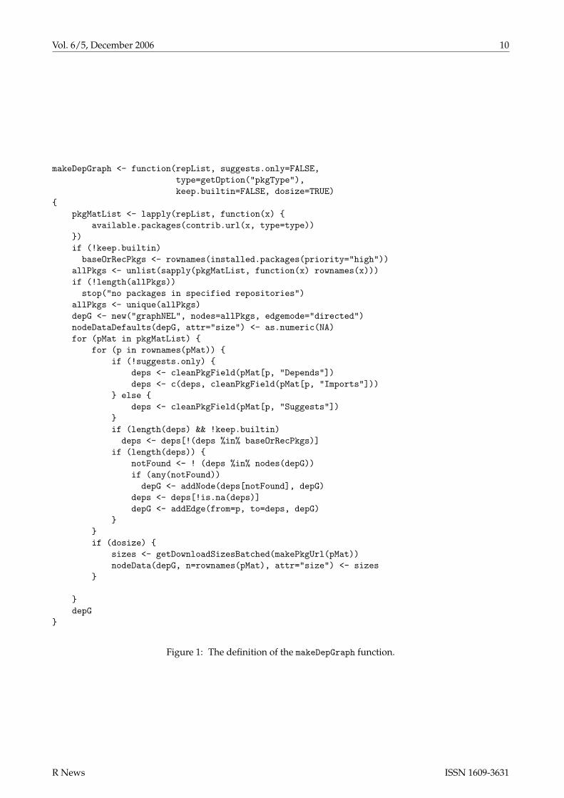
The definition of makeDepGraph is shown inFigure 1. The function obtains a matrix ofpackage meta data from each repository usingavailable.packages. A new graphNEL instance iscreated using new. A node attribute with name “size”is added to the graph with default value NA. Whenkeep.builtin is FALSE (the default), a list of pack-ages that come with a standard R install is retrievedand stored in baseOrRecPkgs.
Iterating through each package’s meta data,the appropriate field (either Depends and Importsor Suggests) is parsed using a helper functioncleanPkgField. If the user has not set keep.builtinto TRUE, the packages that come with R are removedfrom deps, the list of the current package’s depen-dencies. Then for each package in deps, addNode isused to add it to the graph if it is not already present.addEdge is then used to create edges from the pack-age to its dependencies. The size in megabytes ofthe packages in the current repository is retrieved us-ing getDownloadSizesBatched and is then stored asnode attributes using nodeData. Finally, the resultinggraphNEL, depG is returned. A downside of this itera-tive approach to the construction of the graph is thatthe addNode and addEdge methods create a new copyof the entire graph each time they are called. Thiswill be inefficient for very large graphs.
Definitions for the helper functions cleanPkgField,makePkgUrl, and getDownloadSizesBatched are inthe source code of the pkgDepTools package.
Here we use makeDepGraph to build dependencygraphs of the BioC and CRAN packages. Each de-pendency graph is a graphNEL instance. The out-edges of a given node list its direct dependencies(as shown for package annotate). The node attribute“size” gives the size of the package in megabytes.
> biocUrl <- biocReposList()["bioc"]
> cranUrl <- biocReposList()["cran"]
> biocDeps <- makeDepGraph(biocUrl)
> cranDeps <- makeDepGraph(cranUrl)
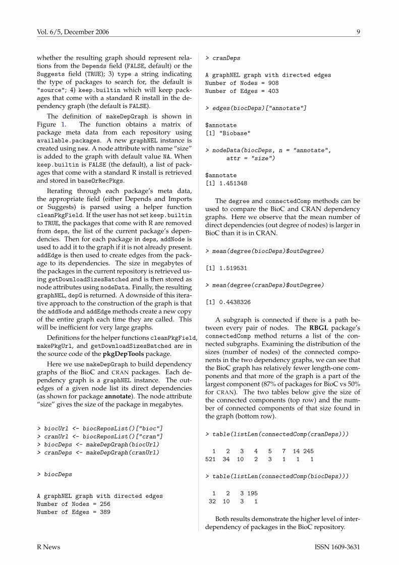
> biocDeps
A graphNEL graph with directed edgesNumber of Nodes = 256Number of Edges = 389
> cranDeps
A graphNEL graph with directed edgesNumber of Nodes = 908Number of Edges = 403
> edges(biocDeps)["annotate"]
$annotate[1] "Biobase"
> nodeData(biocDeps, n = "annotate",
attr = "size")
$annotate[1] 1.451348
The degree and connectedComp methods can beused to compare the BioC and CRAN dependencygraphs. Here we observe that the mean number ofdirect dependencies (out degree of nodes) is larger inBioC than it is in CRAN.
> mean(degree(biocDeps)$outDegree)
[1] 1.519531
> mean(degree(cranDeps)$outDegree)
[1] 0.4438326
A subgraph is connected if there is a path be-tween every pair of nodes. The RBGL package’sconnectedComp method returns a list of the con-nected subgraphs. Examining the distribution of thesizes (number of nodes) of the connected compo-nents in the two dependency graphs, we can see thatthe BioC graph has relatively fewer length-one com-ponents and that more of the graph is a part of thelargest component (87% of packages for BioC vs 50%for CRAN). The two tables below give the size ofthe connected components (top row) and the num-ber of connected components of that size found inthe graph (bottom row).
> table(listLen(connectedComp(cranDeps)))
1 2 3 4 5 7 14 245521 34 10 2 3 1 1 1
> table(listLen(connectedComp(biocDeps)))
1 2 3 19532 10 3 1
Both results demonstrate the higher level of inter-dependency of packages in the BioC repository.
R News ISSN 1609-3631
Vol. 6/5, December 2006 10
makeDepGraph <- function(repList, suggests.only=FALSE,type=getOption("pkgType"),keep.builtin=FALSE, dosize=TRUE)
pkgMatList <- lapply(repList, function(x)
available.packages(contrib.url(x, type=type)))if (!keep.builtin)baseOrRecPkgs <- rownames(installed.packages(priority="high"))
allPkgs <- unlist(sapply(pkgMatList, function(x) rownames(x)))if (!length(allPkgs))stop("no packages in specified repositories")
allPkgs <- unique(allPkgs)depG <- new("graphNEL", nodes=allPkgs, edgemode="directed")nodeDataDefaults(depG, attr="size") <- as.numeric(NA)for (pMat in pkgMatList)
for (p in rownames(pMat)) if (!suggests.only)
deps <- cleanPkgField(pMat[p, "Depends"])deps <- c(deps, cleanPkgField(pMat[p, "Imports"]))
else deps <- cleanPkgField(pMat[p, "Suggests"])
if (length(deps) && !keep.builtin)deps <- deps[!(deps %in% baseOrRecPkgs)]
if (length(deps)) notFound <- ! (deps %in% nodes(depG))if (any(notFound))depG <- addNode(deps[notFound], depG)
deps <- deps[!is.na(deps)]depG <- addEdge(from=p, to=deps, depG)
if (dosize)
sizes <- getDownloadSizesBatched(makePkgUrl(pMat))nodeData(depG, n=rownames(pMat), attr="size") <- sizes
depG
Figure 1: The definition of the makeDepGraph function.
R News ISSN 1609-3631

Vol. 6/5, December 2006 11
Using the Dependency Graph
The dependencies of a given package can be visu-alized using the graph generated by makeDepGraphand the Rgraphviz package. The graph in Figure 2was produced using the code shown below. The accmethod from the graph package returns a vector ofall nodes that are accessible from the given node.Here, it has been used to obtain the complete list ofCategory’s dependencies.
> categoryNodes <- c("Category",
names(acc(biocDeps, "Category")[[1]]))
> categoryGraph <- subGraph(categoryNodes,
biocDeps)
> nn <- makeNodeAttrs(categoryGraph,
shape = "ellipse")
> plot(categoryGraph, nodeAttrs = nn)
Category
Biobase
annotate genefilter graph KEGG GO
Figure 2: The dependency graph for the Categorypackage.
In R , there is no easy to way to preview a givenpackage’s dependencies and estimate the amount ofdata that needs to be downloaded even though theinstall.packages function will search for and in-stall package dependencies if you ask it to by specify-ing dependencies=TRUE. Next we show how to builda function that provides such a “preview” by makinguse of the dependency graph.
Given a plot of a dependency graph like the onefor Category shown in Figure 2, one can devise a sim-ple strategy to determine the install order. Namely,find the packages that have no dependencies, theleaves of the graph, and install those first. Thenrepeat that process on the graph that results fromremoving the leaves from the current graph. Thedownload size is easily computed by retrieving the“size” node attribute for each package in the depen-dency list.
basicInstallOrder <- function(pkg, depG) allPkgs <- c(pkg,
names(acc(depG, pkg)[[1]]))if (length(allPkgs) > 1)
pkgSub <- subGraph(allPkgs, depG)toInst <- tsort(pkgSub)if (!is.character(toInst))stop("depG is not a DAG")
rev(toInst) else
allPkgs
Figure 3: Code listing for the basicInstallOrderfunction.
Figure 3 lists the definition of basicInstallOrder,a function that generates the complete dependen-cies for a given package using the strategy outlinedabove. The tsort function from RBGL performs atopological sort of the directed graph. A topologi-cal sort on a DAG gives an ordering of the nodes inwhich node a comes before b if there is an edge froma to b. Reversing the topological sort yields a validinstall order.
The basicInstallOrder function can be used asthe core of a “preview” function for package installa-tion. The pkgDepTools package provides such a pre-view function called getInstallOrder. This func-tion returns the uninstalled dependencies of a givenpackage in proper install order along with the size,in megabytes, of each package. In addition, the func-tion returns the total expected download size. Belowwe demonstrate the getInstallOrder function.
First, we create a single dependency graph for allCRAN and BioC packages.
> allDeps <- makeDepGraph(biocReposList())
Calling getInstallOrder for package GOstats,we see a listing of only those packages that need tobe installed. Your results will be different based uponyour installed packages.
> getInstallOrder("GOstats", allDeps)
$packages1.45MB 0.22MB 1.2MB
"annotate" "Category" "GOstats"
$total.size[1] 2.87551
When needed.only=FALSE, the complete depen-dency list is returned regardless of what packages arecurrently installed.
> getInstallOrder("GOstats", allDeps,
needed.only = FALSE)
R News ISSN 1609-3631

Vol. 6/5, December 2006 12
$packages0.31MB 17.16MB 1.64MB"graph" "GO" "Biobase"1.45MB 1.29MB 0.23MB
"annotate" "RBGL" "KEGG"0.23MB 0.22MB 1.2MB
"genefilter" "Category" "GOstats"
$total.size[1] 23.739
Wrap Up
We have shown how to generate package depen-dency graphs and preview package installation us-ing the pkgDepTools package. We have described indetail how the underlying code is used and the pro-cess of modeling relationships with the graph pack-age.
These tools can help identify and understand in-terdependencies in packages. A very similar ap-proach can be applied to visualizing class hierarchiesin R such as those implemented using the S4 (Cham-bers, 1998) class system or Bengtsson’s R.oo (Bengts-son, 2006) package.
The graph, RBGL, and Rgraphviz suite of pack-ages provides a very powerful means of manipulat-ing, analyzing, and visualizing relationship data.
Bibliography
H. Bengtsson. R.oo: R object-oriented programmingwith or without references, 2006. URL http://www.braju.com/R/. R package version 1.2.3.
V. Carey and L. Long. RBGL: Interface to boost C++graph lib, 2006. URL http://bioconductor.org. Rpackage version 1.10.0.
J. M. Chambers. Programming with Data: A Guide tothe S Language. Springer-Verlag New York, 1998.
R. Gentleman, E. Whalen, W. Huber, and S. Falcon.graph: A package to handle graph data structures, 2006.R package version 1.12.0.
J. Gentry. Rgraphviz: Provides plotting capabilities for Rgraph objects, 2006. R package version 1.12.0.
E. Hartuv and R. Shamir. A clustering algorithmbased on graph connectivity. Information Process-ing Letters, 76(4–6):175–181, 2000. URL citeseer.ist.psu.edu/hartuv99clustering.html.
M. Kanehisa and S. Goto. KEGG: Kyoto encyclope-dia of genes and genomes. Nucleic Acids Res, 28:27–30, 2000.
Seth FalconProgram in Computational BiologyFred Hutchinson Cancer Research CenterSeattle, WA, [email protected]
Image Analysis for Microscopy ScreensImage analysis and processing with EBImage
by Oleg Sklyar and Wolfgang Huber
The package EBImage provides functionality to per-form image processing and image analysis on large setsof images in a programmatic fashion using the R lan-guage.
We use the term image analysis to describe the ex-traction of numeric features (image descriptors) fromimages and image collections. Image descriptors canthen be used for statistical analysis, such as classifi-cation, clustering and hypothesis testing, using theresources of R and its contributed packages.
Image analysis is not an easy task, and the defi-nition of image descriptors depends on the problem.Analysis algorithms need to be adapted correspond-ingly. We find it desirable to develop and optimizesuch algorithms in conjunction with the subsequentstatistical analysis, rather than as separate tasks. This
is one of our motivations for writing the package.
We use the term image processing for operationsthat turn images into images, with the goals ofenhancing, manipulating, sharpening, denoising orsimilar (Russ, 2002). While some image processingis often needed as a preliminary step for image anal-ysis, image processing is not the primary aim of thepackage. We focus on methods that do not require in-teractive user input, such as selecting image regionswith a pointer etc. Whereas interactive methods canbe extremely effective for small sets of images, theytend to have limited throughput and reproducibility.
EBImage uses the Magick++ interface to theImageMagick (2006) image processing library to im-plement much of its functionality in image process-ing and input/output operations.
R News ISSN 1609-3631

Vol. 6/5, December 2006 13
Cell-based assays
Advances in automated microscopy have made itpossible to conduct large scale cell-based assays withimage-type phenotypic readouts. In such an assay,cells are grown in the wells of a microtitre plate (of-ten a 96- or 384-well format is used) under a condi-tion or stimulus of interest. Each well is treated withone of the reagents from the screening library and theresponse of the cells is monitored, for which in manycases certain proteins of interest are antibody-stainedor labeled with a GFP-tag (Carpenter and Sabatini,2004; Wiemann et al., 2004; Moffat and Sabatini, 2006;Neumann et al., 2006).
The resulting imaging data can be in theform of two-dimensional (2D) still images, three-dimensional (3D) image stacks or image-based timecourses. Such assays can be used to screen com-pound libraries for the effect of potential drugs onthe cellular system of interest. Similarly, RNA inter-ference (RNAi) libraries can be used to screen a setof genes (in many cases the whole genome) for theeffect of their loss of function in a certain biologicalprocess (Boutros et al., 2004).
Importing and handling images
Images are stored in objects of class Image which ex-tends the array class. The colour mode is defined bythe slot rgb in Image; the default mode is grayscale.
New images can be created with the standardconstructor new, or using the wrapper functionImage. The following example code produces a100x100 pixel grayscale image of black and whitevertical stripes:
> im <- Image(0, c(100,100))> im[c(1:20, 40:60, 80:100),,] = 1
By using ImageMagick, the package supportsreading and writing of more than 95 image formatsincluding JPEG, TIFF and PNG. The package canprocess multi-frame images (image stacks, 3D im-ages) or multiple files simultaneously. For example,the following code reads all colour PNG files in theworking directory into a single object of class Image,converts them to grayscale and saves the output as asingle multi-frame TIFF file:
> files <- dir(pattern=".png")> im <- read.image(files, rgb=TRUE)> img <- toGray(im)> write.image(img, "single_multipage.tif")
Besides operations on local files, the package canread from anonymous HTTP and FTP sources, and itcan write to anonymous FTP locations. These proto-cols are supported internally by ImageMagick and donot use R-connections.
The storage mode of grayscale images is double,and all R-functions that work with arrays can be di-rectly applied to grayscale images. This includes thearithmetic functions, subsetting, histograms, Fouriertransformation, (local) regression, etc. For example,the sharpened image in Figure 1c can be obtained bysubtracting the slightly blurred, scaled in colour ver-sion of the original image (Figure 1b) from its sourcein Figure 1a. All pixels that become negative aftersubtraction are then re-set to background. The sourceimage is a subset of the original microscopic image.Hereafter, variables in the code are given the sameliteral names as the corresponding image labels (e.g.data of variable a are shown in Figure 1 a, b – in b,and C – in c, etc).
> orig <- read.image("ch2.png")> a <- orig[150:550, 120:520,]> b <- blur(0.5 * a, 80, 5)> C <- a - b> C[C < 0] = 0> C <- normalize(C)
One can think of this code as of a naive, butfast and effective, version of the unsharp mask fil-ter; a more sophisticated implementation from theImageMagick library is provided by the functionunsharpMask in the package.
Figure 1: Implementation of a simple unsharp maskfilter: (a) source image, (b) blurred colour-scaled im-age, (c) sharpened image after normalization
Some of the image analysis routines assumegrayscale data in the interval [0, 1], but formallythere are no restrictions on the range.
The storage mode of RGB-images is integer, andwe use the three lowest bytes to store red (R), green(G) and blue (B) values, each in the integer-basedrange of [0, 255]. Because of this, arithmetic andother functions are generally meaningless for RGB-images; although they can be useful in some specialcases, as shown in the example code in the followingsection. Support for RGB-images is included to en-hance the display of the analysis results. Most anal-ysis routines require grayscale data though.
Image processing
The ImageMagick library provides a number of imageprocessing routines, so-called filters. Many of thoseare ported to R by the package. The missing ones
R News ISSN 1609-3631

Vol. 6/5, December 2006 14
may be added at a later stage. We have also imple-mented additional image processing routines that wefound useful for work on cell-based assays.
Filters are implemented as functions acting onobjects of class Image and returning a new Image-object of the same or appropriately modified size.One can divide them into four categories: image en-hancement, segmentation, transformation and colour cor-rection. Some examples are listed below.
sharpen, unsharpMask generate sharpened ver-sions of the original image.
gaussFilter applies the Gaussian blur operator tothe image, softening sharp edges and noise.
thresh segments a grayscale image into a binaryblack-and-white image by the adaptive thresh-old algorithm.
mOpen, mClose use erosion and dilation to en-hance edges of objects in binary images and toreduce noise.
distMap performs a Euclidean distance transform ofa binary image, also known as distance map. Ona distance map, values of pixels indicate howfar are they away from the nearest background.Our implementation is adapted from the Scilabimage processing toolbox (SIP Toolbox, 2005)and is based on the algorithm by Lotufo andZampirolli (2001).
normalize shifts and scales colours of grayscale im-ages to a specified range, normally [0, 1].
sample.image proportionally resizes images.
The following code demonstrates how grayscaleimages recorded using three different microscope fil-ters (Figure 2 a, b and c) can be put together intoa single false-colour representation (Figure 2 d), andconversely, how a single false-colour image can bedecomposed into its individual channels.
> files <- c("ch1.png","ch2.png","ch3.png")> orig <- read.image(files, rgb=FALSE)> abc <- orig[150:550, 120:520,]> a <- toGreen(abc[,,1]) # RGB> b <- toRed(abc[,,2]) # RGB> d <- a + b + toBlue(abc[,,3])> C <- getBlue(d) # gray
Figure 2: Composition of a false-colour image (d)from a set of grayscale microscopy images for threedifferent luminescent compounds: (a) – DAPI, (b) –tubulin and (c) – phalloidin
Displaying images
The package defines the method display whichshows images in an interactive X11 window, whereimage stacks can be animated and browsed through.This function does not use R graphics devices andcannot be redirected to any of those. To redi-rect display into an R graphics device, the methodplot.image can be used, which is a wrapper for theimage function from the graphics package. Sinceeach pixel is drawn as a polygon, plot.image ismuch slower compared to display; also, it showsonly the first image of a stack:
> display(abc) # displays all 3> plot.image(abc[,,2]) # can display just 1
Drawables
Pixel values can be set either by using the con-ventional subset assignment syntax for arrays(as in the third code example, C[C < 0] = 0) orby using drawables. EBImage defines the fol-lowing instantiable classes for drawables (de-rived from the virtual Drawable): DrawableCircle,DrawableLine, DrawableRect, DrawableEllipseand DrawableText. The stroke and fill colours, thefill opacity and the stroke width can be set in thecorresponding slots of Drawable. As the opportu-nity arises, we plan to provide drawables for text,poly-lines and polygons. Drawables can be drawnon Images with the method draw; both grayscale andRGB images are supported with all colours automat-ically converted to gray levels on grayscale images.
R News ISSN 1609-3631

Vol. 6/5, December 2006 15
The code below illustrates how drawables can beused to mark the positions and relative sizes of thenuclei detected from the image in Figure 2a. It as-sumes that x1 is the result of the function wsObjects,which uses a watershed-based image segmentationfor object detection. x1 contains matrix objects withobject coordinates (columns 1 and 2) and areas (col-umn 3). The resulting image is shown in Figure 3b.This is just an illustration, we do not assume circularshapes of nuclei. For comparison, the actual segmen-tation boundaries are colour-marked in Figure 3a us-ing the function wsPaint:
> src <- toRGB(abc[,,1])> x <- x1$objects[,1]> y <- x1$objects[,2]> r <- sqrt(x1$objects[,3] / pi)> cx <- DrawableCircle(x, y, r)> b <- draw(src, cx)> a <- wsPaint(x1, src)
Figure 3: Colour-marked nuclei detected with func-tion wsObjects: (a) – as detected, (b) – illustrated byDrawableCircle’s.
Analysing an RNAi screen
Consider an experiment in which images like thosein Figure 2 were recorded for each of ≈ 20,000 genes,using a whole-genome RNAi library to test the ef-fect of gene knock-down on cell viability and appear-ance. Among the image descriptors of interest are thenumber, position, size, shape and the fluorescent in-tensities of cells and nuclei.
The package provides functionality to identifyobjects in images and to extract image descriptors inthe function wsObjects. The function identifies dif-ferent objects in parallel using a modified watershed-based segmentation algorithm and using image dis-tance maps as input. The result is a list of three ma-trix elements objects, pixels (indices of pixels con-stituting the objects) and borders (indices of pixelsconstituting the object boundaries). If the suppliedimage is an image stack, the result is a list of suchlists. Each row in the matrix objects correspondsto a detected object, with different object descriptorsin the columns: x and y coordinates, size, perimeter,number of pixels on the image edge, acircularity, ef-fective radius, perimeter to radius ratio, etc. Objects
on the image edges can be automatically removed ifthe ratio of the detected edge pixels to the perimeteris larger than a given threshold. If the original image,from which the distance map was calculated, is spec-ified in the argument ref, the overall intensity of theobject region is calculated as well.
For every gene, the image analysis workflowlooks, therefore, as follows: load and normalize im-ages, segment, enhance the segmented images bymorphological opening and closing, generate dis-tance maps, identify cells and nuclei, extract imagedescriptors, and, finally, generate image previewswith the identified objects marked.
Object descriptors can then be analysed statisti-cally to cluster genes by their phenotypic effect, gen-erate a list of genes that should be studied further inmore detail (hit list), e.g., genes that have a specificphenotypic effect of interest, etc. The image previewscan be used to verify and audit the performance ofthe algorithm through visual inspection.
A schematic implementation is illustrated in thefollowing example code and in Figure 4. Here weomit the step of nuclei detection (object x1), fromwhere the matrix of nuclei coordinates (object seeds)is retrieved to serve as starting points for the cell de-tection. The nuclei detection is done analogously tothe cell detection without specifying starting points.
> for (X in genes) + files <- dir(pattern=X)+ orig <- read.image(files)+ abc <- normalize(orig, independent=TRUE)+ i1 <- abc[,,1]+ i2 <- abc[,,2]+ i3 <- abc[,,3]+ a <- sqrt(normalize(i1 + i3))+ b <- thresh(a, 300, 300, 0.0, TRUE)+ C <- mOpen(b, 1, mKernel(7))+ C <- mClose(C, 1, mKernel(7))+ d <- distMap(C)+ # x1 <- wsObjects(...) - nuclei detection+ seeds <- x1$objects[,1:2]+ x2 <- wsObjects(d, 30, 10, .2, seeds, i3)+ rgb <- toGreen(i1)+toRed(i2)+ toBlue(i3)+ e <- wsPaint(x2, rgb, col="white",fill=F)+ f <- wsPaint(x2, i3, opac = 0.15)+ f <- wsPaint(x1, f, opac = 0.15)+
Note that here we adopted the record-at-a-time ap-proach: image data, which can be huge, are storedon a mass-storage device and are loaded into RAMin portions of just a few images at a time.
Summary
EBImage brings image processing and image anal-ysis capabilities to R. Its focus is the programmatic
R News ISSN 1609-3631

Vol. 6/5, December 2006 16
(non-interactive) analysis of large sets of similar im-ages, such as those that arise in cell-based assays forgene function via RNAi knock-down. Image descrip-tors can be analysed further using R’s functionalitiesin machine learning (clustering, classification) andhypothesis testing.
Our current work on this package focuses onmore accurate object detection and algorithms forfeature/descriptor extraction. Image registration,alignment and object tracking are of foreseeable in-terest. In addition, one can imagine many otheruseful features, for example, support for moreImageMagick functions, better display options (e.g.,using GTK) or interactivity. Contributions or collab-orations on these or other topics are welcome.
Figure 4: Illustration of the object detection algo-rithm: (a) – sqrt-brightened combined image of nu-clei (DAPI from Figure 2a) and cells (phalloidin fromFigure 2c); (b) – image a after blur and adaptive thresh-olding; (c) – image b after morphological opening fol-lowed by closing; (d) – normalized distance map gen-erated from image c; (e) – outlines of cells detectedusing wsObjects drawn on top of the RGB imagefrom Figure 2d; (f) – colour-mapped cells and nucleias detected with wsObjects (one unique colour perobject)
Installation
The package depends on ImageMagick, which needsto be present on the system to install the package.
Please refer to the ‘INSTALL’ file.
Acknowledgements
We thank F. Fuchs and M. Boutros for providingtheir miscroscopy data and for many stimulatingdiscussions about the technology and the biology,R. Gottardo and F. Swidan for testing the package onMacOS X and the European Bioinformatics Institute(EBI), Cambridge, UK, for financial support.
Bibliography
M. Boutros, A. Kiger, S. Armknecht, et al. Genome-wide RNAi analysis of cell growth and viability inDrosophila. Science, 303:832–835, 2004.
A. E. Carpenter and D.M. Sabatini. Systematicgenome-wide screens of gene function. Nature Re-views Genetics, 5:11–22, 2004.
ImageMagick: software to convert, edit, and com-pose images. Copyright: ImageMagick Studio LLC,1999-2006. URL http://www.imagemagick.org/
R. Lotufo and F. Zampirolli. Fast multidimensionalparallel Euclidean distance transform based onmathematical morphology. SIBGRAPI-2001/Brazil,100–105, 2001.
J. Moffat and D.M. Sabatini. Building mammaliansignalling pathways with RNAi screens. NatureReviews Mol. Cell Biol., 7:177–187, 2006.
B. Neumann, M. Held, U. Liebel, et al. High-throughput RNAi screening by time-lapse imag-ing of live human cells. Nature Mathods, 3(5):385–390, 2006.
J. C. Russ. The image processing handbook – 4th ed.CRC Press, Boca Raton. 732 p., 2002
SIP Toolbox: Scilab image processing toolbox.Sourceforge, 2005. URL http://siptoolbox.sourceforge.net/
S. Wiemann, D. Arlt, W. Huber, et al. From ORFeometo biology: a functional genomics pipeline. GenomeRes. 14(10B):2136–2144, 2004.
Oleg Sklyar and Wolfgang HuberEuropean Bioinformatics InstituteEuropean Molecular Biology LaboratoryWellcome Trust Genome CampusHinxton, CambridgeCB10 1SDUnited [email protected]; [email protected]
R News ISSN 1609-3631

Vol. 6/5, December 2006 17
beadarray: An R Package to AnalyseIllumina BeadArraysby Mark Dunning*, Mike Smith*, Natalie Thorne, andSimon Tavaré
Introduction
Illumina have created an alternative microarray tech-nology based on randomly arranged beads, each ofwhich carries copies of a gene-specific probe (Kuhnet al., 2004). Random sampling from an initial pool ofbeads produces an array containing, on average, 30randomly positioned replicates of each probe type.A series of decoding hybridisations is used to iden-tify each bead on an array (Gunderson et al., 2004).The high degree of replication makes the gene ex-pression levels obtained using BeadArrays more ro-bust. Spatial effects do not have such a detrimentaleffect as they do for conventional arrays that providelittle or no replication of probes over an array. Illu-mina produce two distinct BeadArray technologies;the SAM (Sentrix Array Matrix) and the BeadChip.A SAM is a 96-well plate arrangement containing 96uniquely prepared hexagonal BeadArrays, each con-taining around 1500 bead types. The BeadChip tech-nology comprises a series of rectangular strips on aslide with each strip containing around 24,000 beadtypes. The most commonly used BeadChip is theHumanRef-6 BeadArray. These have 6 pairs of strips,each pair having 24,000 RefSeq genes and 24,000 sup-plemental genes.
Until now, analysis of BeadArray data has beencarried out by using Illumina’s own software pack-age (BeadStudio) and therefore does not utilise thewide range of bioinformatic tools already availablevia Bioconductor (Gentleman et al., 2004), such aslimma (Smyth, 2005) and affy (Gautier et al., 2004).Also, the data output from BeadStudio only gives asingle average for each bead type on an array. Thuspotentially interesting information about the repli-cates is lost. The intention of this project is to createan R package, beadarray, for the analysis of BeadAr-ray data incorporating ideas from existing Biocon-ductor packages. We aim to provide a flexible andextendable means of analysing BeadArray data bothfor our own research purposes and for the benefit ofother users of BeadArrays. The beadarray packageis able to read the full bead level data for both SAMand BeadChip technologies as well as bead summarydata processed by BeadStudio. The package includesan implementation of Illumina’s algorithms for im-age processing, although local background correc-tion and sharpening are optional.
At present, beadarray is a package for the analy-
sis of Illumina expression data only. For the analysisof Illumina SNP data, see the beadarraySNP packagein Bioconductor.
Data Formats
1 TIFF Image + 1 BeadLevel csv file for eacharray
BeadScan software
BeadStudioGUI
Raw Data
QC Data
Sample Sheet
BeadLevelList ExpressionSetIllumina
~30 values perbead typeImage processingoptional
1 value per beadtypePre-Processed data
limma, affy etc,….
beadarray
Figure 1: Diagram showing the interaction be-tween beadarray and Illumina software. Variousfunctions from Bioconductor packages (eg., limmaand affy) may be used for the pre-processingor downstream analysis of BeadLevelList orExpressionSetIllumina objects.
After hybridisation and washing, each SAM orBeadChip is scanned by the BeadScan software toproduce a TIFF image for each array in an experi-ment. The size of each TIFF image is around 6Mb and80Mb for SAM and BeadChip arrays respectively.BeadScan will also provide a text file describing theidentity and position of each bead on the array if re-quested (version 3.1 and above of BeadScan only).We call this the bead level data for an array. Notethat the bead level text file has to be produced whenthe arrays are scanned and cannot be generated lateron. BeadStudio is able to read these raw data andproduce a single intensity value for each bead typeafter outliers are excluded. These values are referredto as bead summary data. The images are processedusing a local background correction and sharpeningtransformation (Dunning et al., 2005). These stepsare not optional within the BeadStudio software. Thebead summary values calculated by BeadStudio canbe output directly with or without normalisation ap-plied or used for further analysis within the appli-cation. The output from BeadStudio also containsinformation about the standard error of each beadtype, the number of beads and a detection score that
1These authors contributed equally to this work.
R News ISSN 1609-3631
Vol. 6/5, December 2006 18
measures the probablity that the bead type is ex-pressed; this uses a model assumed by Illumina. Allanalysis within BeadStudio is done on the unloggedscale and using the bead summary values rather thanfull replicate information for each bead type. Figure1 gives an overview of the interaction between thefile formats and software involved in the analysis ofBeadArray data.
Bead Level Analysis
The readBeadLevelData function is used to readbead level data. A targets object is used in a simi-lar way to limma to define the location of the TIFFimages and text files. Both SAM and BeadChip datacan be read by readBeadLevelData. The default op-tions for the function use the sharpening transforma-tion recommended by Illumina and calculate a lo-cal background value for each bead. The usage ofreadBeadLevelData is:
> BLData = readBeadLevelData(targets,
+ imageManipulation="sharpen")
> slotNames(BLData)
[1] "G" "R" "Rb" "Gb"[5] "GrnY" "GrnX" "ProbeID" "targets"
Even though the size of the TIFF images is ratherlarge, readBeadLevelData uses C code to read theseimages quickly, taking around 2 seconds to processeach SAM array and 1 minute for each BeadChiparray on a 3Ghz Pentium c©IV machine with 3Gbof RAM. An object of type BeadLevelList is re-turned by readBeadLevelData. The design of thisclass is similar to the RGList object used in limma.Note that we store the foreground (G) and back-ground (Gb) intensities of each bead separately sothat local background correction is optional using thebackgroundCorrect function. Each bead on the ar-ray has a ProbeID that defines the bead type for thatbead. We order the rows in the matrix according tothe ProbeID of beads, making searching for beadswith a particular ProbeID more efficient. The GrnXand GrnY matrices give the coordinates of each beadcentre on the original TIFF image. Note that the ran-dom nature of BeadArrays means that the number ofreplicates of a particular bead type will vary betweenarrays and rows in the matrices will not always cor-respond to the same bead type, unlike data objectsfor other microarray technologies.
Typical quality control steps for conventional mi-croarrays involve looking for systematic differencesbetween arrays in the same experiment and also forlarge spatial effects on each array. The boxplot func-tion can be easily applied to the foreground or back-ground values to reveal possible defective arrays. We
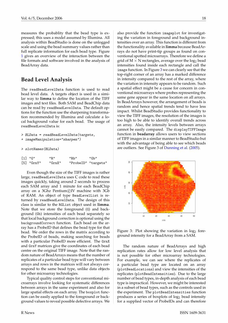
also provide the function imageplot for investigat-ing the variation in foreground and background in-tensities over an array. This function is different fromthe functionality available in limma because BeadAr-rays do not have print-tip groups as found on con-ventional spotted microarrays. Therefore we define agrid of M × N rectangles, average over the log2 beadintensities found inside each rectangle and call theimage function. In Figure 3 we can clearly see that thetop-right corner of an array has a marked differencein intensity compared to the rest of the array, wherethe variation in intensity appears to be random. Sucha spatial effect might be a cause for concern in con-ventional microarrays where probes representing thesame gene appear in the same location on all arrays.In BeadArrays however, the arrangement of beads israndom and hence spatial trends tend to have lessimpact. Whilst BeadStudio provides functionality toview the TIFF images, the resolution of the images istoo high to be able to identify overall trends acrossan array. Also, the intensity levels between arrayscannot be easily compared. The displayTIFFImagefunction in beadarray allows users to view sectionsof TIFF images in a similar manner to BeadStudio butwith the advantage of being able to see which beadsare outliers. See Figure 3 of Dunning et al. (2005).
10 20 30 40 50
1020
3040
50
1:51
1:51
Figure 3: Plot showing the variation in log2 fore-ground intensity for a BeadArray from a SAM.
The random nature of BeadArrays and highreplication rates allow for low level analysis thatis not possible for other microarray technologies.For example, we can see where the replicates ofa particular bead type are located on an array(plotBeadLocations) and view the intensities of thereplicates (plotBeadIntensities). Due to the largenumber of bead types, in-depth analysis of each beadtype is impractical. However, we might be interestedin a subset of bead types, such as the controls used inthe experiment. The plotBeadIntensities functionproduces a series of boxplots of log2 bead intensityfor a supplied vector of ProbeIDs and can therefore
R News ISSN 1609-3631

Vol. 6/5, December 2006 19
Figure 2: beadarray can be used to find spatial effects on arrays. On the left is a representation of the numberof outliers for each array (bright red indicates more outliers) and on the right is the location of outliers for aparticular array. Clicking on a hexagon on the left will change which array is displayed on the right. For thisfigure, the array in the 7th column of the first row of the SAM was chosen.
be a useful diagnostic tool.Another set of beads that are of interest are out-
liers. Illumina exclude outliers for a particular beadtype using a cut-off of 3 MADs from the unloggedmean. This analysis can be repeated for all beadtypes on an array using the findAllOutliers func-tion. Users may specify a different cut-off as a multi-ple of the MAD or use the log2 intensity of beads inthis function. Note that the outliers are not removedfrom the analysis at this point. To find all the outliersfor every bead type on the first array we would use:
> o = findAllOutliers(BLData, array=1)
The result is a vector that indexes the rows of thefirst array in BLData. The plotBeadLocations func-tion can then be used to plot the location of the out-liers on the array.
> plotBeadLocations(BLData, array=1,
BeadIDs=o)
Typically, we find that 5% of beads on arrays areoutliers and this can be used as an ad-hoc criterionfor quality control. Figure 2 shows one of the inter-active features available within beadarray. The leftside of the screen gives an overview of all arrays ona SAM or BeadChip. In this example, each array iscoloured according to the number of outliers and im-mediately we can see which arrays on the SAM havea larger number of outliers (shown in bright red).
By clicking on a particular array in the graphic dis-play, the location of all outliers on that array will bedisplayed on the right of the screen. This exampleshows the same array seen in Figure 3. As one mightexpect, many of the outliers in Figure 2 correspond toareas of higher foreground intensity visible in Figure3.
Alternatively, the foreground or background in-tensities of arrays may be used to colour the ar-rays in the left screen and imageplots such as Fig-ure 3 can be displayed when individual arrays areclicked. This interactive functionality is available forboth SAM and BeadChip bead level data and canbe started by the SAMSummary and BeadChipSummaryfunctions respectively with the BeadLevelList cre-ated by readBeadLevelData passed as a parameter.
The createBeadSummaryData function createsbead summary data for each array by removing out-liers for a particular bead type and then taking an av-erage of the remaining beads. The findAllOutliersfunction is used by default and the result is anExpressionSetIllumina object which can be anal-ysed using different functionality within beadarray.
Reading Pre-Processed Bead Sum-mary Data
Bead Summary data processed by BeadStudiocan be read into beadarray using the functionreadBeadSummaryData. Three separate input files are
R News ISSN 1609-3631

Vol. 6/5, December 2006 20
required by the function, the location of which can bespecified by a targets text file. The first two files areautomatically created by BeadStudio by selecting theGene Analysis option whereas the third file must becreated by the user.
• Raw Data file - This contains the raw, non-normalised bead summary values as output byBeadStudio. Inside the file are several linesof header information followed by a data ma-trix. Each row is a different probe in the ex-periment and the columns give different mea-surements for the probes. For each array,we record the summarised expression level(AVG_Signal), standard error of the bead repli-cates (BEAD_ST_DEV), Number of beads used(Avg_NBEADS) and a Detection score whichestimates the probability of a gene being de-tected above the background. Note that whilstthis data has not been normalised, it has beensubjected to local background correction at thebead level prior to summarising.
• QC Info - Gives the summarised expressionvalues for each of the controls that Illuminaplace on arrays and hence is useful for diagnos-tic purposes. Each row in the file is a differentarray and the columns give average expression,standard error and detection for various con-trols on the array. See Illumina documentationfor descriptions of control types.
• Sample Sheet - Gives a unique identifier toeach array and defines which samples were hy-bridised to each array.
An example Bead Summary data set is includedwith the beadarray package and can be found as azipped folder in the beadarray download. Thesedata were obtained as part of a pilot study intoBeadArray technology and comprises 3 HumanRef-6BeadChips with various tumour and normal sampleshybridised. The following code can be used to readthe example data into R.
> targets <-
readBeadSummaryTargets("targets.txt")
> BSData <- readBeadSummaryData(targets)
> BSData
Instance of ExpressionSetIllumina
assayDataStorage mode: listDimensions:
BeadStDev Detection exprs NoBeadsFeatures 47293 47293 47293 47293Samples 18 18 18 18
phenoData
rowNames: I.1, IC.1,..., Norm.2, (18 total)varLabels and descriptions:
featureDatafeatureNames: GI_10047089-S,...(47293 total)varLabels and descriptions:
Experiment dataExperimenter name:Laboratory:Contact information:Title:URL:PMIDs:No abstract available.
Annotation [1] "Illumina"QC InformationAvailable Slots: Signal StDev DetectionfeatureNames: 1475542110_F,...1475542113_FsampleNames: Biotin, ..negative
The output of readBeadSumamryData is an objectof type ExpressionSetIllumina which is an exten-sion of the ExpressionSet class developed by the Bio-core team used as a container for high-throughputassays. The data from the raw data file has beenwritten to the assayData slot of the object, whereasthe phenoData slot contains information from sam-ple sheet and the QC slot contains the quality con-trol information. For consistency with the definitionof other ExpressionSet objects, we use exprs andse.exprs to access the expression and standard er-ror slots.
Analysis of Bead Summary Data
The quality control information read as part ofreadBeadSummaryData can be retrieved using QCInfoand plotted using plotQC, which gives an overviewof each control type. Plots of particular controls(e.g., negative controls) can be produced usingsingleQCPlot with the usual R plotting argumentsavailable.
Scatter and M (difference) vs. A (average) plotscan be generated for multiple arrays using theplotMAXY function (Figure 4). These can give a vi-sual indicator of the variability between arrays in anexperiment. For replicate arrays, we would expect tosee the majority of points lying on the horizontal forthe MA plots and along the diagonal for the scatterplots. Systematic deviation from these lines may in-dicate a bias between the arrays which requires nor-malising. An MA or scatter plot can also be producedfor just two arrays at a time (plotMA and plotXY re-spectively). An attractive feature of these plots is thatthe location of particular genes (e.g., controls) can behighlighted using the genesToLabel argument.
R News ISSN 1609-3631

Vol. 6/5, December 2006 21
0.6 0.8 1.0 1.2 1.4
−1.
0−
0.5
0.0
0.5
1.0
Index
IH−1
8 10 12 14
8 10 12 14
−2
−1
01
2
68
1012
14
0.6 0.8 1.0 1.2 1.4
−1.
0−
0.5
0.0
0.5
1.0
Index
0 IC−1
−2
−1
01
2
8 10 12 14 16
68
1012
14
8 10 12 14 16 0.6 0.8 1.0 1.2 1.4
−1.
0−
0.5
0.0
0.5
1.0
0 IH−2
Figure 4: The plotMAXY function can be used to compare bead summary data from multiple arrays in the sameexperiment. In this figure we compare three replicates from the example bead summary data provided withbeadarray
R News ISSN 1609-3631
Vol. 6/5, December 2006 22
Since the ExpressionSetIllumina class includesa matrix of expression values, it can be analysed ina similar manner to data obtained from other tech-nologies. In particular, this enables normalisationof BeadArray data to be carried out using the exist-ing methods available in other Bioconductor pack-ages (such as those available within the affy pack-age, using assayDataElementReplace to replace theexprs slot). Illumina recommend normalising databy subtracting the average value of negative controlsfrom each array. This method is implemented in thebackgroundNormalise function and has quite a dra-matic effect at lower intensities, often producing a lotof negative values. Typically, we find that the vari-ability between arrays is low and a quantile or me-dian normalisation (the function medianNormalisein beadarray) is sufficient.
The linear modelling tools within limma (Smyth,2004) can be applied to the log-transformed expres-sion exprs matrix in order to detect genes which aredifferentially expressed between arrays. The Illu-mina custom method is implemented by the functionDiffScore but at present is only able to make pair-wise comparisons between arrays.
Computational Issues and FuturePlans
The vast amounts of data that can be generatedfrom BeadArray experiments present a number ofchallenges for researchers, especially for analysesbased on the bead level data. One has to con-sider that there are 12 80MB TIFF images foreach BeadChip and 96 6MB TIFF Images for aSAM. In the case of a BeadChip experiment, sim-ply reading the data into R for arrays from morethan one BeadChip is problematic. We find thatat least 1 Gb of RAM is required to run thereadBeadLevelData and createBeadSummaryDatafunctions on a BeadLevelList object representingone BeadChip. We hope to implement methods fornormalisation which take the full bead level infor-mation into account but anticipate that this is goingto be a computationally expensive task and may re-quire the package to take advantage of parallel com-puting tools for R. Future versions of the package willalso have better methods for creating bead averageswhich take information from replicate arrays into ac-count.
Another major addition planned for beadarray isto allow sequence annotation information to be im-ported so that Illumina expression data can be com-bined with other microarray technologies such as ar-rayCGH, SNP and DNA methylation arrays. Weplan to include functionality to read Illumina SNPand methylation data into the package.
Useful Illumina Resources
The vignettes supplied with the package give moredetailed examples of how to analyse both bead leveland bead summary data. Our previous paper (Dun-ning et al., 2005) provides descriptions of the imageprocessing steps used by Illumina and some exam-ples of bead level analysis. Readers interested in acomparison between Illumina and Affymetrix tech-nologies are referred to Barnes et al. (2005).
We are keen to hear comments and feedback fromusers of beadarray.
Acknowledgements
We thank Brenda Kahl and Semyon Kruglyak (Illu-mina), Barbara Stranger, Matthew Forrest and Mano-lis Dermitzakis (Wellcome Trust Sanger Institute),and Andrew Lynch and John Marioni (Universityof Cambridge) for many helpful discussions duringthe devlopment of this work. We would also liketo thank Isabelle Camilier (Ecole Polytechnique) forimplementing the Illumina image processing algo-rithms and Roman Sasik (University of California,San Diego) for providing C code for reading TIFF im-ages. The authors were supported by grants fromCancer Research UK (MS, NT & ST) and the Medi-cal Research Council (MD). Simon Tavaré is a RoyalSociety / Wolfson Research Merit Award holder.
Bibliography
MJ Dunning, NP Thorne, I Camilier, et al. Qual-ity control and low-level statistical analysis of Il-lumina BeadArrays. Revstat, 4:1–30, 2006.
RC Gentleman, VJ Carey, DM Bates, et al. Bioconduc-tor: open software development for computationalbiology and bioinformatics. Genome Biol, 5:R80,2004.
KL Gunderson, S Kruglyak, MS Graige, et al. Decod-ing randomly ordered DNA arrays. Genome Res,14:870–877, 2004.
K Kuhn, SC Baker, E Chudin, et al. A novel, high-performance random array platform for quanti-tative gene expression profiling. Genome Res,14:2347–2356, 2004.
L Gautier, L Cope, BM Bolstad, et al. affy–analysisof Affymetrix GeneChip data at the probe level.Bioinformatics, 20(3):307–15, 2004.
GK Smyth. Linear models and empirical Bayes meth-ods for assessing differential expression in mi-croarray experiments. Statistical Applications in Ge-netics and Molecular Biology, 3:113–136, 2004.
R News ISSN 1609-3631

Vol. 6/5, December 2006 23
GK Smyth. Limma: linear models for microarraydata. In R Gentleman, V Carey, W Huber, et al.Bioinformatics and Computational Biology Solutionsusing R and Bioconductor, pages 397–420. Springer,New York, 2005.
M Barnes, J Freudenberg, S Thompson, et al. Ex-perimental comparison and cross-validation of theAffymetrix and Illumina gene expression analysisplatforms. Nucleic Acids Res, 33:5914–5923, 2005.
Mark Dunning, Mike Smith, Natalie Thorne and SimonTavaréComputational Biology GroupHutchison / MRC Research CentreDepartment of OncologyUniversity of CambridgeHills Rd, Cambridge CB2 2XZUnited [email protected]@[email protected]@damtp.cam.ac.uk
Transcript Mapping with High-DensityTiling Arraysby Matthew Ritchie and Wolfgang Huber
Introduction
Oligonucleotide tiling arrays allow the measurementof transcriptional activity and DNA binding eventsat a much higher resolution than traditional microar-rays. Compared to the spotted technology, tiling ar-rays typically contain between 10 and 1000 times asmany probes, which may be ordered or ‘tiled’ alongentire chromosomes, or within specific regions of in-terest, such as promoters.
For RNA analysis, tiling arrays can be used toidentify novel transcripts, splice variants, and anti-sense transcription (Bertone et al., 2004; Stolc et al.,2005). In DNA analysis, this technology can iden-tify DNA binding sites through chromatin immuno-precipitation (ChIP) on chip analysis (Sun et al.,2003; Carroll et al., 2005) or genetic polymorphismsand chromosomal rearrangements via comparativegenome hybridization (arrayCGH).
Due to the wide range of applications of this tech-nology and the custom nature of the probe layout,the analysis of these data is different to that of regu-lar microarrays. In this article, the tilingArray pack-age, which extends the existing Bioconductor toolsetto the problem of measuring transcriptional activityusing Affymetrix high-density tiling arrays, is pre-sented.
Background
The initial processing steps of quality assessmentand normalization which are routinely applied tolower density arrays are also important when ana-lyzing tiling array data. Diagnostic plots of the rawprobe intensity data can highlight systematic biases
or artefacts which may warrant the need for individ-ual arrays or batches of arrays to be repeated. Nor-malization between arrays is necessary when datafrom multiple hybridizations is to be combined in ananalysis. In the tilingArray package, a normaliza-tion method which uses the probe intensities froma DNA hybridization as a reference is implemented(Huber et al., 2006). The next step in the analy-sis is to detect the transcript boundaries. A sim-ple change-point model, which segments the orderedchromosomal intensity data into discrete units hasproven quite useful for whole genome tiling arraydata (David et al., 2006). Other approaches whichuse Hidden Markov Models (Toyoda and Shinozaki,2005; Munch et al., 2006) or moving averages (Schadtet al., 2004) have also been proposed. Displaying thedata with reference to the position along the chro-mosome allows visualization of the segmentation re-sults. These capabilities will be demonstrated in thefollowing sections.
The custom Affymetrix arrays used in this arti-cle were produced for the Stanford Genome Tech-nology Center and tile the complete genome of Sac-charomyces cerevisiae with 25mer probes arranged insteps of 8 bases along both strands of each chro-mosome. The two tiles per chromosome are off-set by 4 bases (see Figure 1). Both perfect match(PM) and mismatch (MM) probes were available.The experimental data we analyze comes from Davidet al. (2006), and includes 5 RNA hybridizations fromyeast cells undergoing exponential growth and 3DNA hybridizations of labelled genomic fragments.This data is publicly available in the davidTilingpackage or from ArrayExpress (accession number E-TABM-14). A cell cycle experiment made up of RNAhybridizations from 24 time-points sampled at 10minute intervals and 3 DNA hybridizations will alsobe used.
R News ISSN 1609-3631

Vol. 6/5, December 2006 24
25mer
8bp
4bp
3’5’
3’ 5’
Watson strand
Crick strand
Figure 1: Probe spacing for Saccharomyces cerevisiaetiling arrays. The 25 mer probes are offset by 8 basesand tile each strand of DNA.
Reading data
We assume that the .CEL files from the davidTilingpackage are unzipped and available in the R work-ing directory. To read in these data, the followingcommands can be used.
> library("tilingArray")
> cels = dir(pattern = ".cel")
> e = readCel2eSet(cels, rotated = TRUE)
The readCel2eSet function is is a wrapper forReadAffy from the affy package. Rotating the .CELfile data through 90 degrees clock-wise by settingrotated=TRUE was necessary for these arrays due toold scanner settings. The data can also be loadedwith
> library("davidTiling")
> data("davidTiling")
> dim(davidTiling)
Features Samples6553600 8
The 8 arrays each contain 6,553,600 probes arrangedin a grid with 2560 rows x 2560 columns. A specialdata structure is necessary for the mapping betweenthe probes on the array and their target regions inthe genome. For the yeast tiling array, we use an en-vironment, named probeAnno, which organizes thisinformation in two ways. Firstly, for each chromoso-mal strand, a vector of probe identifiers, in linear ge-nomic order, and the coordinates and type of matchis stored. In addition, the type of match and identi-fier of its hit region (e.g. YBR275C) are stored in theorder that the probes appear on the array. To load,and find out further details about this environment,type
> data("probeAnno")
> ? probeAnno
To create this environment, the probes were mappedto the yeast genome using the MUMmer program(Delcher et al., 2002). In order to screen out ambigu-ous probes from the analysis, probes with multiplematches to the yeast genome where flagged and dis-carded from the analysis.
Users who wish to apply the tilingArray pack-age to other types of tiling arrays, for example, fromother species, need to produce their own probeAnno-like environment. Currently, there is no support fordoing this. An objective of future work is to makethis process and the genome mapping data struc-tures more generic. We aim to use the infrastructurethat will be provided by the oligo package for thispurpose.
Once the data has been imported, some simplediagnostic plots can be generated with
> qcPlots(davidTiling, probeAnno = probeAnno)
This command generates an HTML report with im-age plots, box plots and density plots of log base 2intensity data in the current working directory.
Normalization
The tilingArray package implements aDNA based normalization strategy in thenormalizeByReference function. Normalization ofthe davidTiling data is carried out with the follow-ing commands
> isDNA = davidTiling$nucleicAcid ==
+ "genomic DNA"
> isRNA = davidTiling$nucleicAcid ==
+ "poly(A) RNA"
> pm = PMindex(probeAnno)
> bg = BGindex(probeAnno)
> yn = normalizeByReference(davidTiling[,
+ isRNA], reference = davidTiling[,
+ isDNA], pm = pm, background = bg)
The logical vectors isDNA and isRNA indicate whicharrays are DNA and RNA hybridizations respec-tively. The intensities measured on the DNA hy-bridizations are used for two purposes. First, theprobes indexed by the bg vector are used to estimatethe background signal. Second, the PM intensities(indexed by the pm vector) provide a reference signalwhich is used to correct for probe specific responsesdue to base content. Once the PM intensities fromthe RNA hybridizations have been adjusted for back-ground signal and probe effects, variance-stabilizingnormalization between arrays using the vsn function(Huber et al., 2002) is applied to the data. For detailsof the method, see Huber et al. (2006).
R News ISSN 1609-3631
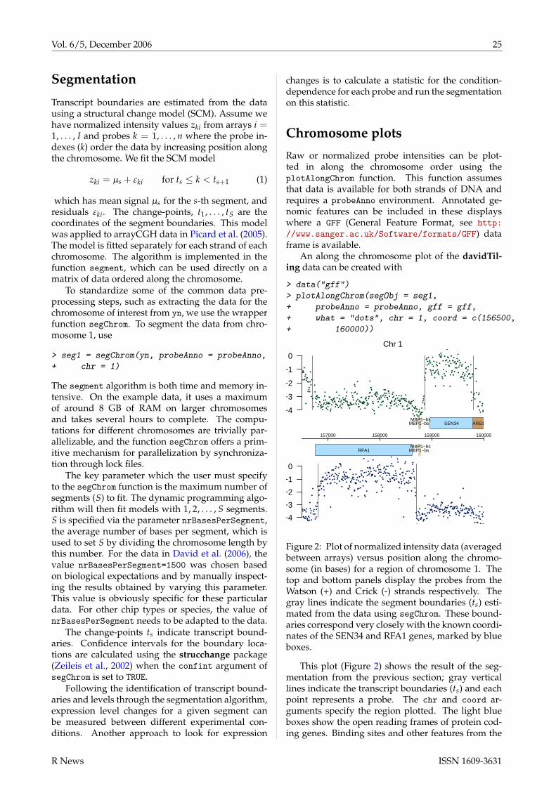
Vol. 6/5, December 2006 25
Segmentation
Transcript boundaries are estimated from the datausing a structural change model (SCM). Assume wehave normalized intensity values zki from arrays i =1, . . . , I and probes k = 1, . . . , n where the probe in-dexes (k) order the data by increasing position alongthe chromosome. We fit the SCM model
zki = µs +εki for ts ≤ k < ts+1 (1)
which has mean signal µs for the s-th segment, andresiduals εki. The change-points, t1, . . . , tS are thecoordinates of the segment boundaries. This modelwas applied to arrayCGH data in Picard et al. (2005).The model is fitted separately for each strand of eachchromosome. The algorithm is implemented in thefunction segment, which can be used directly on amatrix of data ordered along the chromosome.
To standardize some of the common data pre-processing steps, such as extracting the data for thechromosome of interest from yn, we use the wrapperfunction segChrom. To segment the data from chro-mosome 1, use
> seg1 = segChrom(yn, probeAnno = probeAnno,
+ chr = 1)
The segment algorithm is both time and memory in-tensive. On the example data, it uses a maximumof around 8 GB of RAM on larger chromosomesand takes several hours to complete. The compu-tations for different chromosomes are trivially par-allelizable, and the function segChrom offers a prim-itive mechanism for parallelization by synchroniza-tion through lock files.
The key parameter which the user must specifyto the segChrom function is the maximum number ofsegments (S) to fit. The dynamic programming algo-rithm will then fit models with 1, 2, . . . , S segments.S is specified via the parameter nrBasesPerSegment,the average number of bases per segment, which isused to set S by dividing the chromosome length bythis number. For the data in David et al. (2006), thevalue nrBasesPerSegment=1500 was chosen basedon biological expectations and by manually inspect-ing the results obtained by varying this parameter.This value is obviously specific for these particulardata. For other chip types or species, the value ofnrBasesPerSegment needs to be adapted to the data.
The change-points ts indicate transcript bound-aries. Confidence intervals for the boundary loca-tions are calculated using the strucchange package(Zeileis et al., 2002) when the confint argument ofsegChrom is set to TRUE.
Following the identification of transcript bound-aries and levels through the segmentation algorithm,expression level changes for a given segment canbe measured between different experimental con-ditions. Another approach to look for expression
changes is to calculate a statistic for the condition-dependence for each probe and run the segmentationon this statistic.
Chromosome plots
Raw or normalized probe intensities can be plot-ted in along the chromosome order using theplotAlongChrom function. This function assumesthat data is available for both strands of DNA andrequires a probeAnno environment. Annotated ge-nomic features can be included in these displayswhere a GFF (General Feature Format, see http://www.sanger.ac.uk/Software/formats/GFF) dataframe is available.
An along the chromosome plot of the davidTil-ing data can be created with
> data("gff")
> plotAlongChrom(segObj = seg1,
+ probeAnno = probeAnno, gff = gff,
+ what = "dots", chr = 1, coord = c(156500,
+ 160000))
−4
−3
−2
−1
0
MBP1−bsMBP1−bs
SEN34 ARS101
−4
−3
−2
−1
0
RFA1 MBP1−bsMBP1−bs
157000 158000 159000 160000
Chr 1
Figure 2: Plot of normalized intensity data (averagedbetween arrays) versus position along the chromo-some (in bases) for a region of chromosome 1. Thetop and bottom panels display the probes from theWatson (+) and Crick (-) strands respectively. Thegray lines indicate the segment boundaries (ts) esti-mated from the data using segChrom. These bound-aries correspond very closely with the known coordi-nates of the SEN34 and RFA1 genes, marked by blueboxes.
This plot (Figure 2) shows the result of the seg-mentation from the previous section; gray verticallines indicate the transcript boundaries (ts) and eachpoint represents a probe. The chr and coord ar-guments specify the region plotted. The light blueboxes show the open reading frames of protein cod-ing genes. Binding sites and other features from the
R News ISSN 1609-3631

Vol. 6/5, December 2006 26
gff data frame are also marked on the figure in therelevant locations. The absolute level of expressionfor different transcripts can be visualized in this dis-play.
The following commands can be used to generatea heatmap display of the normalized intensities fromthe cell cycle data set (available in the object cycle),for the same region on chromosome 1 as in Figure 2.
> plotAlongChrom(y=cycle,+ probeAnno=probeAnno, gff=gff,+ what="heatmap", chr=1,+ coord=c(156500,160000))
Figure 3 shows the resulting output. The periodic ex-pression patterns for the cell cycle regulated SEN34and RFA1 transcripts are clearly visible in this figure.
020406080
100120140160180200220
MBP1−bsMBP1−bs
SEN34 ARS101
020406080
100120140160180200220
RFA1 MBP1−bsMBP1−bs
157000 158000 159000 160000
Chr 1
Figure 3: Heatmap plot of probe intensities from acell cycle experiment for a region of chromosome1. Each row in the y-direction displays the normal-ized intensities from a different time-point (0 min-utes through to 230 minutes). The x-axis shows theposition along the chromosome (in bases). The color-scheme indicates the intensity level, ranging fromlight yellow for lower intensities, through to darkblue for higher intensities.
Summary
The tilingArray package provides tools for read-ing, normalizing, segmenting and visualizingAffymetrix tiling array data. The core functions arenormalizeByReference and segment, and their un-derlying methodology is described in Huber et al.(2006). These functions should be widely applicableto tiling array data.
There are also some functions and objectsthat have been customized to our specific Sac-charomyces cerevisiae data sets, such as segChrom,plotAlongChrom and probeAnno. These functionscan be used as templates for transferring the meth-ods to other types of arrays and species, but this willrequire some work by the user. In future releases, wehope to use the infrastructure for tiling array datathat will be offered by the oligo package to makethese tools more generic.
Many exciting, open research questions still re-main including a data-driven approach for selectingan optimal number of segments (S) for each chro-mosome (Huber et al., 2006), applying SCMs beyondpiece-wise constant curves and the segmentation ofcondition-dependent transcription patterns.
Acknowledgements
We thank Jörn Tödling and Zhenyu Xu for contribu-tions to the development of the tilingArray package,Lior David, Marina Granovskaia, Sandra Clauder-Münster and Lars Steinmetz for providing the dataused in this article, Eugenio Mancera for Figure 1 andRachel Uren for proof-reading the article.
Bibliography
P. Bertone, V. Stolc, T. E. Royce et al. Global identifica-tion of human transcribed sequences with genometiling arrays. Science, 306(5705):2242–2246, 2004.
J. S. Carroll, X. S. Liu, A. S. Brodsky et al.Chromosome-wide mapping of estrogen receptorbinding reveals long-range regulation requiringthe forkhead protein FoxA1. Cell, 122:33–43, 2005.
L. David, W. Huber, M. Granovskaia et al. Ahigh-resolution map of transcription in the yeastgenome. Proc Natl Acad Sci USA, 103(14):5320–5325, 2006.
A. L. Delcher, A. Phillippy, J. Carlton and S. L.Salzberg. Fast algorithms for large-scale genomealignment and comparison. Nucleic Acids Res, 30(11):2478–2483, 2002.
W. Huber, A. V. Heydebreck, H. Sültmann et al. Vari-ance stabilization applied to microarray data cal-ibration and to the quantification of differentialexpression. Bioinformatics, 18(Suppl 1):S96–S104,2002.
W. Huber, J. Toedling and L. M. Steinmetz. Transcriptmapping with oligonucleotide high-density tilingarrays. Bioinformatics, 22(16):1963–1970, 2006.
K. Munch, P. Gardner, P. Arctander and A. Krogh. Ahidden Markov model approach for determiningexpression from genomic tiling micro arrays. BMCBioinformatics, 7:239, 2006.
R News ISSN 1609-3631

Vol. 6/5, December 2006 27
F. Picard, S. Robin, M. Lavielle et al. A statistical ap-proach for array CGH data analysis. BMC Bioinfor-matics, 6(1):27, 2005.
E. E. Schadt, S. W. Edwards, D. GuhaThakurta et al.A comprehensive transcript index of the humangenome generated using microarrays and compu-tational approaches. Genome Biol, 5(10):R73, 2004.
V. Stolc, M. Samanta, W. Tongprasit et al. Identi-fication of transcribed sequences in Arabidopsisthaliana by using high-resolution genome tiling ar-rays. Proc Natl Acad Sci USA, 102(12):4453–4458,2005.
L. V. Sun, L. Chen, F. Greil et al. Protein-DNA in-teraction mapping using genomic tiling path mi-croarrays in Drosophila. Proc Natl Acad Sci USA,100:9428–9433, 2003.
T. Toyoda and K. Shinozaki. Tiling array-drivenelucidation of transcriptional structures based on
maximum-likelihood and Markov models. Plant J,43(4):611–621, 2005.
A. Zeileis, F. Leisch, K. Hornik and C. Kleiber. struc-change: An R package for testing for structuralchange in linear regression models. Journal of Sta-tistical Software, 7:1–38, 2002.
Matt RitchieEuropean Bioinformatics Insitute (EBI)European Molecular Biology Laboratory (EMBL) Cam-bridge, [email protected]
Wolfgang HuberEuropean Bioinformatics Insitute (EBI)European Molecular Biology Laboratory (EMBL) Cam-bridge, [email protected]
Analyzing Flow Cytometry Data withBioconductorby Nolwenn Le Meur and Florian Hahne
Introduction
In the recent past, flow cytometry (FCM) has becomea high-throughput technique used in both basic andclinical research. Applications range from studies fo-cusing on the immunological status of patients, ther-apeutic approaches involving stem cells up to func-tional screens used to identify specific phenotypes.The technology is capable of measuring multiple flu-orescence as well as some morphological propertiesof individual cells in a cell population on the basisof light emission. FCM experiments can be extremelycomplex to analyze due to the large volume of datathat is typically created in several processing steps.As an example, flow cytometry high content screen-ing (FC-HCS) can process at a single workstation upto a thousand samples per day each containing thou-sands of cells, monitoring up to eighteen parametersper sample. Thus, the amount of information gener-ated by these technologies must be stored and man-aged and finally needs to be summarized in order tomake it accessible to the researcher.
Instrument manufacturers have developed soft-ware to drive the data acquisition process of theircytometers, but these tools are primarily designedfor their proprietary instrument interface and offerfew or no high level data processing functions. Thepackages rflowcyt and prada provide facilities for
importing, storing, assessing and preprocessing datafrom FCM experiments. In this article we demon-strate the use of these packages for some commontasks in flow cytometry data analysis.
FCS format
In order to facilitate data exchange across differ-ent platforms, a data standard has been developedwhich is now widely accepted by the flow cytometrycommunity and also by most instrument manufac-turers. Flow Cytometry Standard (FCS) binary filescontain both raw data and accompanying meta dataof individual cytometry measurements and option-ally the results of prior analyses carried out on theraw data (Seamer et al., 1997). The current versionof the FCS standard is 3.0, but both packages can alsodeal with the old 2.0 standard which is still widelyused. We can import FCS files into R using the func-tion read.fcs.
Data models
Both rflowcyt and prada use their own object modelsto deal with FCM data. While the focus of rflowcytis more on single cytometry measurements, pradaoffers the possibility to combine several individualmeasurements in the confines of a single experiment
R News ISSN 1609-3631

Vol. 6/5, December 2006 28
and to include all the necessary metadata. Its objectmodel tries to stay close to the familiar micro-arraydata structures (expressionSet) making use of al-ready defined generic functions. Both models storethe data corresponding to the different immunoflu-orescence measurements or variables and the meta-data included in the FCS files. The 2 main slots pro-vide:
• a data frame with rows corresponding to thebiological unit (i.e. cells) and columns corre-sponding to the measured variables
• the experimental metadata as a list (rflowcyt)or a named vector (prada)
The argument objectModel to read.fcs can be usedto chose between the two models when importingthe data. In addition, the package rflowcyt providesfunctions for the conversion between objects of bothclasses.
prada data model
Objects of class cytoFrame are the containers for stor-ing individual cytometry measurements in prada.The data slot can be accessed using the func-tion exprs, the metadata slot via the functiondescription. Subsetting of the data is possible us-ing the usual syntax for data frames and matrices.
> library(prada)
> data(cframe)
> cframe
cytoFrame object with 2115 cells and 8 observables:
FSC-H SSC-H FL1-H FL2-H FL3-H FL2-A FL4-H Time
slot ’description’ has 148 elements
> subset <- cframe[1:3, c(1, 2,
+ 3, 7, 8)]
> exprs(subset)
FSC-H SSC-H FL1-H FL4-H Time[1,] 467 532 87 449 2[2,] 437 431 28 478 2[3,] 410 214 0 358 2
> description(cframe)[4:6]
$SYS"Macintosh System Software 9.2.2"
CREATOR"CellQuest Pro 4.0.2"
$TOT"2115"
Collections of several cytometry measurements(whole experiments) can be stored in objects of classcytoSet. The phenoData slot of these objects con-tains all the relevant experiment-wide meta data.Multiple FCS files can be imported along with their
metadata when the first argument to read.fcs is avector of filenames or an object of class phenoData(see the documentation to read.fcs for more de-tails). Subsetting of cytoSets is similar to subsettingof list, i.e., individual cytoFrame objects are returnedwhen subsetting is done with double brackets.
> data(cset)
> cset
cytoSet object with 5 cytoFrames and colnames
FSC-H SSC-H FL1-H FL2-H FL3-H FL2-A FL4-H Time
> subset <- cset[1:2]
> pData(subset)
name ORF2 fas-Bcl2-plate323-04-04.A02 MOCK3 fas-Bcl2-plate323-04-04.A03 YFPbatch
2 13 1
> class(cset[[3]])
[1] "cytoFrame"attr(,"package")[1] "prada"
csApply can be used to apply a function on allitems of a cytoSet. In a simple case this could forinstance be a preprocessing step or a statistical in-ference on the data from each well. In a more com-plex application, the function could summarize dif-ferent features of the data and even produce diag-nostic plots for visualization and quality assesment.Here, we apply a preprocessing function which re-moves artefactual measurements from our datasetbased on the morphological properties of a cell andcomputes the number of cells in each of the wells onthe plate.
> myFun <- function(xraw)
+ fn <- fitNorm2(xraw[, c("FSC-H",
+ "SSC-H")], scale = 2)
+ x <- xraw[fn$sel, ]
+ return(nrow(x))
+
> cellCounts <- csApply(cset,
+ myFun)
Many of the common R methods like plotor length are also available for objects of classcytoFrame and cytoSet.
rflowcyt data model
Objects of class FCS are the containers for storing in-dividual cytometry measurements in rflowcyt. Thedata slot can be accessed using the function fluors,the metadata slot via the function metaData. Subset-ting of the data is possible using:
R News ISSN 1609-3631

Vol. 6/5, December 2006 29
• [i,j] to extract or subset information from thedata (a matrix object) of the FCS R-object
• [[i]] to extract metadata (which is of S4 class FC-Smetadata) of the FCS R-object
> library(rflowcyt)> data(VRCmin)> st.DRT
Original Object of class FCS from:DRT_GAG.fcsObject name: st.DRTDimensions 206149 by 8
> subset <- st.DRT[1:3,1:3]> metaData(subset)
FACSmetadata for non-original FCS object:st.DRT from original file DRT_GAG.fcswith 3 cells and 3 parameters.
> fluors(subset)FSC-Height Side Scatter CD8 FITC
1 640 458 2982 136 294 1023 588 539 265
Multiple cytometry measurements can be im-ported when the filename argument to read.fcs isa vector of file names and are stored as a list of in-dividualFCS objects. These lists may be further pro-cessed using the familiar basic R functions, however,no experiment-wide metadata is provided.
Besides the FCS class, rflowcyt includeFCSmetadata, FCSsummary, and FCSgate classes.FCSmetadata is the class of the metadata slot of anFCS R-object. The FCSsummary class is the class ofthe output of the summary method implemented ona FCS R-object. The FCSgate class contains the FCSclass and extends it to include gating information(for more details, see the following section).
Gating
A common task in the analysis of flow cytome-try data is to perform interactive selections of sub-populations of cells with respect to one or severalmeasurement parameters, a process known as gat-ing. In this respect, a gate is a set of rules thatuniquely identifies a cell to be part of a given sub-population. In the easiest case this can be a sharpcutoff, e.g., all cells with values in one parameter thatare larger than a given threshold. But often muchmore complex selections are necessary like rectangu-lar or elliptic areas in two dimensions or even polyg-onal boundaries. It is sometimes desirable to definea gate on a data set and later on apply this gate to anumber of additional data sets, hence gates should
be independent from the actual raw data. In addi-tion, there may be several different combinations ofgates that can be combined in a logical manner (i.e.,“AND” and “OR”) and in a defined order, thus theconcept of the gate can be extended to collections ofmultiple gates.
The package prada offers the infrastructure toapply gating on cytometry data. Objects of classgate and gateSet model the necessary featuresof individual gates and of collections of multiplegates and can be assigned to the gate slot of ob-jects of class cytoFrame. Gates can either be cre-ated from scratch by specifying the necessary se-lection rules or, much more conveniently, the func-tion drawGate can be used to interactively set gatesbased on two-dimensional scatter plots of the rawdata (Fig. 1). Please see the vignette of packageprada for a more thorough discussion on gating.
Figure 1: Interactive drawing of a polygonal gatebased on a scatterplot of two cytometry parametersusing function drawGate.
Quality control and quality assess-ment of cytometry data
Data quality control and quality assessment are cru-cial steps in processing high throughput FCM data.Quality control efforts have been made in clinical cellanalysis by flow cytometry. For example, guidelineswere defined to monitor the fluorescence measure-ments by computing calibration plots for each flu-orescent parameter. However such procedures arenot yet systematically applied in high throughputFCM and quality assessment of the raw data is oftenneeded to overcome the lack of data quality control.The aim of data quality assessment is to detect sys-tematic and stochastic effects that are not likely to bebiologically motivated. The rationale is that system-atic errors often indicate the need for adjustmentsin sample handling or processing. Further, the aber-
R News ISSN 1609-3631

Vol. 6/5, December 2006 30
rant samples should be identified and potentiallyremoved from any downstream analysis in order toavoid spurious results.
rflowcyt proposes a variety of graphical ex-ploratory data analytic (EDA) tools to explore andsummarize ungated FCM data.
• plotECDF.FCS creates Empirical CumulativeDistribution (ECDF) plots that reveal differ-ences in distributions (Fig. 2);
• boxplot.FCS draws boxplots that display loca-tion and variation of the distributions and facil-itate the comparison of these features betweensamples as they are aligned horizontally;
• plotQA.FCS summarizes the distribution of oneor two parameters by their means, medians,modes or IQR for the diferent samples and dis-plays the values in a scatterplot (Fig. 4). Thedots in the resulting scatterplot can be coloredaccording to the samples position in a 96-wellplate to reveal potential plate effects;
• plotdensity.FCS displays density curves thatreveal the shape of the distributions, especiallymulti-modality and asymmetry;
We illustrate the usefulness of those visualizationtools to assess FCM data quality through examina-tion of a collection of weekly peripheral blood sam-ples obtained from a patient following allogeneicblood and marrow transplant. Samples were takenat various time points before and after transplanta-tion. At each time point, every blood sample wasdivided into eight aliquots. Values for the forwardlight scatter (FSC) which measures a cell’s size andfor the sideward light scatter (SSC, a measure for acell’s granularity) of aliquots from the same sampleshould therefore be comparable.
The plotECDF.FCS function can be used to visual-ize several variables for several samples in the samegraph.
> data(flowcyt.data)
> subset <- flowcyt.data[c(1:24,
+ 41:48, 57:72)]
> stain <- paste("A", 1:8, sep = "")
> timePoint <- c(-8, 0, 5, 27,
+ 39, 46)
> plotECDF.FCS(subset,+ varpos = c(1),+ var.list = c(paste("Day ",+ timePoint)),+ group.list = stain,+ type = "l", xlab = "FSC",+ lwd = 2, cex = 1.5)
For example, Figure 2 shows the FSC parame-ter for the 8 aliquots of a sample per time point.Each panel corresponds to a particular time point,in days before or after transplantation. In Figure 2we expected to see the density curves superimpose.One aliquot significantly deviates from the other.This aliquot should be investigated in more detailand potentially be removed from further analysis.
FSC
Em
piric
al c
umul
ativ
e di
strib
utio
n
0.0
0.2
0.4
0.6
0.8
1.0Day −8
0 200 600 1000
Day 0 Day 5
0 200 600 1000
Day 27 Day 39
0 200 600 1000
0.0
0.2
0.4
0.6
0.8
1.0Day 46
A1A2
A3A4
A5A6
A7A8
Figure 2: ECDF plots of the FSC parameter for 8aliquots of a sample at different time point. Eachpanel corresponds to a particular time point, in daysbefore or after transplantation. In each panel, eachintensity curves represents one of the 8 aliquots.
ECDF plots are not good for visualizing the shapeof the distributions. Instead, you can use the functionplotdensity.FCS (Fig. 3).
0 200 400 600 800 1000
0.00
00.
005
0.01
00.
015
FSC Intensity
Den
sity
Figure 3: Density plots of the FSC parameter for 8aliquots of the same sample.
R News ISSN 1609-3631

Vol. 6/5, December 2006 31
> plotdensity.FCS(subset[41:48],
+ varpos = c(1), ylab = "Density",
+ xlab = "FSC Intensity",
+ col = c(1:8), ylim = c(0,
+ 0.015))
Finally the plotQA.FCS function creates "sum-mary" scatterplots to visualize samples relationshipwithin plates. This representation allows to identifybiological outlier and/or plate biases, such as edgeeffect or within-plate spatial effect. Figure 4 showsthe SSC vs FSC median intensities for all aliquotsstored in one 96-well plate and colored by their col-umn position in the plate. In this figure, if all sam-ples were identical, we expect to see a single clusterof data points. One has to be careful when interpret-ing such plots as each column correspond to differentsamples collected at different time points. However,we note that some columns have widely spread val-ues (light blue and brown) and that one aliquot is anoutlier as it is far away from the rest of its group. Thisaliquot appears to be the same as in Figures 2 and 3.
> idx <- order(names(flowcyt.data))
> flowcyt.data <- flowcyt.data[idx]
> plotQA.FCS(flowcyt.data, varpos = c(1,
+ 2), col = "col", median,
+ labeling = TRUE, xlab = "SSC median",
+ ylab = "FSC median", xlim = c(0,
+ 200), ylim = c(75, 275),
+ pch = "*", asp = 1, cex = 1.5,
+ main = "")
**
**
*
*
**
*
*
*
**
***
*
*
**
*
*
***
***
*
*
**
**
**
**
***
*
**
*
*
***
***
*
*
**
**
**
**
**
*
*
* *
**
**
**
**
*
*
* *
**
**
**
**
*
*
* *
**
**
0 50 100 150 200
100
150
200
250
SSC median
FS
C m
edia
n
a01
a02
a03a04
a05
a06
a07a08
a09
a10
a11
a12
b01
b02
b03b04
b05
b06
b07b08
b09
b10
b11
b12c01
c02
c03c04
c05
c06
c07c08
c09
c10
c11
c12
d01
d02
d03d04
d05
d06
d07d08
d09
d10
d11d12
e01
e02
e03e04
e05
e06
e07e08
e09
e10
e11
e12
f01
f02
f03
f04
f05
f06
f07 f08
f09
f10
f11
f12
g01
g02
g03g04
g05
g06
g07 g08
g09
g10
g11
g12
h01
h02
h03h04
h05
h06
h07 h08
h09
h10
h11
h12
Figure 4: Scatterplot of SSC vs FSC medians intensi-ties for one plate.
prada offers another visualization tool which canbe used to inspect the data from whole experiments.Using the function plotPlate we can display quan-titative as well as qualitative values or even complexgraphs for each well of a microtiter plate retaining its
array format 2. This allows for the identification ofspatial effects and for a consise presentation of im-portant features of an experiment. plotPlate is im-plemented using grid graphic and users are able todefine their own plotting functions, so conceptuallyanything can be plotted in a mircrotiter plate format(see Figure 5).
0.22
0.42
0.61
0.8
1 2 3 4 5 6 7 8 9 10 11 12
A
B
C
D
E
F
G
H
cell number
1 2 3 4 5 6 7 8 9 10 11 12
A
B
C
D
E
F
G
H
relative local density
Figure 5: Two different variations of plate plotsfor 96 well microtiter plates. Top: Quantitative val-ues. The consistently low number of cells aroundthe edges of the plate indicates a technical prob-lem. Bottom: Complex graph. Image maps of two-dimensional local densities of FSC vs SSC values foreach well relative to a standard. Blue areas indicatelow, red areas indicate high local densities. Theseplots help detect morphological changes in a cellpopulation.
Discussion and Conclusion
The application of flow cytometry in modern cell bi-ology is diverse and so are the demands on data anal-ysis. The multitude of packages within R and Bio-conductor already provides for many tools that arealso useful in the analysis of FCM data. The pack-ages rflowcyt and prada try to close the gap betweendata acquisition and data analysis by enabling the re-searches to take their data into the powerful R envi-ronment and to make use of the statistical and graph-ical solutions already available there. In addition,they provide for tools that are commonly used inearly steps of data analysis which in principle are the
R News ISSN 1609-3631

Vol. 6/5, December 2006 32
same for all FCM applications.Currently, in a collaboration of several groups in-
volved in high-throughput FCM together with instru-ment manufacturers and members of the flow cytom-etry standards initiative a flowCore package and anumber of additional FCM utility packages are de-veloped. The aim is to merge both prada and rflow-cyt into one core package which is copmpliant withthe data exchange standards that are currently de-veloped in the community. Visualization as well asquality control will than be part of the utility pack-ages that depend on the data structures defined inthe flowCore package.
Bibliography
L. C. Seamer, C. B. Bagwell, L. Barden et al. Proposednew data file standard for flow cytometry, versionfcs 3.0. Cytometry, 28(2):118–122, Jun 1997.
Nolwenn Le MeurComputational BiologyFred Hutchinson Cancer Research CenterSeattle, WA, [email protected]
Florian HahneMolecular Genome AnalysisGerman Cancer Research CenterHeidelberg, [email protected]
Protein Complex Membership Estimationusing apComplexby Denise Scholtens
Graphs of protein-protein interactions, so called ‘in-teractomes’, are rapidly surfacing in the systems bi-ology literature. In these graphs, nodes representcellular proteins and edges represent interactions be-tween them. Global interactome analyses are oftenundertaken to explore topological features such asnetwork diameter, clustering coefficients, and nodedegree distribution. Local interactome modeling,particularly at the protein complex level, is alsoimportant for identifying distinct functional com-ponents of the cell and studying their interactivity(Hartwell et al., 1999). The apComplex package con-tains functions to locally estimate protein complexmembership as described in Scholtens and Gentle-man (2004) and Scholtens et al. (2005).
Two technologies are generally used to queryprotein-protein relationships. Affinity purification-mass spectrometry (AP-MS) technologies detect pro-tein complex co-membership. In these experimentsa set of proteins are used as baits, and in separatepurifications, each bait identifies all hits with whichit shares protein complex membership. AP-MS baitsand their hits may physically bind to each other, orthey may be joined together in a complex through anintermediary protein or set of proteins. If a bait pro-tein is a member of more than one complex, all ofits hits may not necessarily themselves be complexco-members. These biological realities become essen-tial components of complex membership estimation.
Publicly available AP-MS data sets for Saccharomycescerevisiae include those reported by Gavin et al. (2002,2006), Ho et al. (2002), and Krogan et al. (2004, 2006).
Yeast-two-hybrid (Y2H) technology is anotherbait-hit system that measures direct physical interac-tions. The distinction between AP-MS and Y2H datais subtle, but crucial. Two proteins that are part of thesame complex may not physically interact with eachother. Thus an interaction detected by AP-MS maynot be detected by Y2H. On the other hand, two pro-teins that do physically interact by definition form acomplex so any interaction detected by Y2H shouldalso be detected by AP-MS. Under the same exper-imental conditions, Y2H technology should in factconsist of a subset of the interactions detected by AP-MS technology, the subset consisting of complex co-members that are physically bound to each other. Itoet al. (2001) and Uetz et al. (2000) both offer publiclyavailable Y2H data sets for Saccharomyces cerevisiae.
apComplex deals strictly with data resultingfrom AP-MS experiments. The joint analysis of Y2Hand AP-MS data is an interesting and importantproblem and is in fact an obvious next step aftercomplex membership estimation, but is not currentlydealt with in apComplex.
R News ISSN 1609-3631

Vol. 6/5, December 2006 33
Protein Complex Membership andCo-Membership
apComplex estimates protein complex membershipgiven a set of AP-MS co-membership data. Thedistinction between the complex membership andco-membership ties back to affiliation relationshipsin social networks analyses (Wasserman and Faust,1999). As a simple example to be discussed through-out this article, suppose proteins P1, P2, P4, and P6compose complex C1 and proteins P3, P4, and P5compose complex C2. Then their affiliation matrix,A, is as follows.
C1 C2P1 1 0P2 1 0
A = P3 0 1P4 1 1P5 0 1P6 1 0
A can also be represented as a bipartite graph inwhich one set of nodes represent proteins, anotherset represents complexes, and edges from proteins tocomplexes denote complex membership.
Instead of A, AP-MS technology assays Y = A⊗A′ where ⊗ represents matrix multiplication underthe Boolean algebra 0 + 0 = 0× 0 = 1× 0 = 0× 1 =0 and 1 + 0 = 0 + 1 = 1 + 1 = 1 × 1 = 1. Entriesof 1 in Y represent co-membership of two proteinsin a complex. In this simple example, we have Y asfollows.
P1 P2 P3 P4 P5 P6P1 1 1 0 1 0 1P2 1 1 0 1 0 1
Y = P3 0 0 1 1 1 0P4 1 1 1 1 1 1P5 0 0 1 1 1 0P6 1 1 0 1 0 1
apComplex estimates A using assays of Y.
Observed Data
The entire matrix Y is not tested in AP-MS experi-ments. For this to happen, all cellular proteins wouldneed to be used as baits. Even in small model organ-isms such as Saccharomyces cerevisiae with approxi-mately 6000 cellular proteins, genome-wide testing islogistically prohibitive. Instead, only a subset of therows of Y are tested (letting rows represent baits andcolumns represent hits). In a graph of Y, this is bestdescribed by neighborhood sampling of all edges ex-tending from baits to all other proteins. Recognitionof this sampling scheme is crucial as it draws a very
important distinction between two types of edgesthat are absent from a graph of AP-MS data. Figure 1shows ideal results from a neighborhood sampling ofour simple interactome using P1, P2, and P3 as baits.The edge between P1 and P3 is tested and observed tobe absent, but the edge between P4 and P6 is absentbecause it is never tested. Scholtens and Gentleman(2004) discuss why inference should only be basedon the tested edges, leaving the untested edges to beestimated or tested in further experiments.
P1
P2 P3
P4 P5P6
Figure 1: Co-memberships detected using neighbor-hood sampling scheme with P1, P2, and P3 as baits.
In addition to being incomplete AP-MS data arealso imperfect, including both false positive (FP) andfalse negative (FN) observations. Figure 2 demon-strates hypothetical FP observations from P8 to P3and P3 to P7 and a FN observation from P2 to P4.
P1
P2
P3
P4 P5
P6
P7
P8
Figure 2: Observed data including FPs and FNs.
Penalized Likelihood Approach
Since edges in an AP-MS graph represent complexcomembership, if all proteins were used as baits,then maximal complete subgraphs (or cliques) inthe AP-MS graph would contain entire collectionsof proteins that compose a complex. The maximalcomplete subgraphs could then be used to estimateA (see Scholtens and Gentleman, 2004 and Scholtenset al., 2005 for a more thorough discussion).
Since all proteins are not used as baits, apCom-plex instead searches for maximal BH-complete sub-graphs in the observed AP-MS data. A BH-completesubgraph is defined to be a collection of baits andhits for which all bait-bait edges and all bait-hit-onlyedges exist; a maximal BH-complete subgraph is a BH-complete subgraph that is not contained in any other
R News ISSN 1609-3631

Vol. 6/5, December 2006 34
BH-complete subgraph. In other words, all edges ob-served in the neighborhood sampling scheme mustexist for a subgraph to be BH-complete. The func-tion bhmaxSubgraph can be used to find maximal BH-complete subgraphs in the observed AP-MS data.
In the event of unreciprocated observations be-tween pairs of baits, the edges are estimated to ex-ist when the sensitivity of the AP-MS technologyis less than the specificity. Under a logistic regres-sion model where the parameters represent sensitiv-ity and specificity, this treatment of unreciprocatedbait-bait edges maximizes the likelihood L for thedata (Scholtens and Gentleman, 2004).
For our example, bhmaxSubgraph reports fourmaximal BH-complete subgraphs as shown below.Figure 3 depicts the bipartite graph of the results con-tained in BP1.
> apEXP1 P2 P3 P8 P4 P5 P6 P7
P1 1 1 0 0 1 0 1 0P2 1 1 0 0 0 0 1 0P3 0 0 1 0 1 1 0 1P8 0 0 1 1 0 0 0 0> BP1 <- bhmaxSubgraph(apEX)
bhmax1 bhmax2 bhmax3 bhmax4P1 0 1 1 0P2 0 1 0 0P3 1 0 0 1P8 1 0 0 0P4 0 0 1 1P5 0 0 0 1P6 0 1 1 0P7 0 0 0 1
BHM1 BHM2BHM3BHM4
P1 P2P3 P4P5 P6P7P8
Figure 3: Bipartite graph for the initial estimate of Adetermined by locating maximal BH-complete sub-graphs in the graph of observed AP -MS data.
The initial maximal BH-complete subgraph esti-mate of A does not allow missing edges between baitand hit-only proteins; since AP-MS technology is notperfectly sensitive, it is reasonable to expect a num-
ber of missing edges in the subgraph for each com-plex estimate. mergeComplexes accommodates thisby employing a penalty term with the likelihood. Fora complex ck, let C(ck) represent the product of 1)the binomial probability for the number of observededges in ck given the number of tested edges and thesupposed sensitivity of the technology, and 2) a two-sided p-value from Fisher’s exact test for the distri-bution of missing incoming edges for complex esti-mate ck. Then let C equal the product of C(ck) overall complexes c1, ..., cK. The penalized likelihood P isthe product of L and C, or P = L×C. L is maximizedwith the initial maximal BH-complete subgraphs –the algorithm in mergeComplexes looks to increase Cin favor of small decreases in L.
After the initial estimate of A is made usingbhmaxSubgraph, mergeComplexes proposes pairwiseunions of individual complex estimates. If P in-creases when the complexes are treated as one, thenthe combination is accepted. If more than oneunion increases P, then the union with the largestincrease is accepted. This is a greedy algorithmand mergeComplexes can be sensitive to the order inwhich the columns in the input matrix are specified.Users may want to order the columns putting the ini-tial complex estimates with more bait proteins firstsince these contain proportionately more tested data.
> BP2 <- mergeComplexes(BP1, apEX,sensitivity = 0.7, specificity = 0.75)> BP2
Complex1 Complex2 Complex3P1 0 1 0P2 0 1 0P3 1 0 1P8 1 0 0P4 0 1 1P5 0 0 1P6 0 1 0P7 0 0 1
Figure 4 shows the corresponding bipartite graphfor the estimated A.
C1 C2C3
P1 P2P3 P4P5 P6P7P8
Figure 4: Bipartite graph for new complex estimatesafter using mergeComplexes.
The function findComplexes can be used to runboth steps together. It will automatically reorder
R News ISSN 1609-3631
Vol. 6/5, December 2006 35
the input to mergeComplexes as suggested previ-ously. Note that the user must specify the sensitiv-ity and specificity of the AP-MS technology. Speci-ficity should be considered in light of the dimensionof the data under consideration. In our small exam-ple, a fairly high FP rate (i.e. low specificity) createsa reasonable number of suspected FP interactions. Inlarge dimensional data sets, the number of true neg-ative interactions is quite large. In these cases, verylow FP probabilities (e.g. 0.001 or specificity=0.999)are usually appropriate.
Algorithm Output
apComplex makes three types of complex estimates:multi-bait-mult-edge (MBME) complexes that con-tain multiple baits and multiple edges, single-bait-multi-hit (SBMH) complexes that contain a singlebait and a collection of hit-only proteins, and un-reciprocated bait-bait (UnRBB) complexes that onlycontain two bait proteins connected by one unrecip-rocated edge. MBME complexes are the most reliablesince they contain the most tested data. SBMH com-plexes are useful for proposing future experimentssince the topology among the hit-only proteins isunknown. UnRBB complexes may result from FPobservations since the edges are tested twice, ob-served once, and not confirmed by other subgraphedges. On the other hand, the unreciprocated edgemay also result from a FN observation between thetwo baits. The complex estimates resulting frommergeComplexes or findComplexes can be sortedinto the MBME, SBMH, and UnRBB components us-ing the function sortComplexes.
Results for three publicly available data sets areincluded in apComplex. TAP is an adjacency matrixof the AP-MS data (called ‘TAP’) reported by Gavin,et al. (2002). There were 3420 comemberships re-ported using 455 baits and 909 hit-only proteins. TheTAP data were originally compiled into 232 yTAPcomplexes, available in Supplementary Table 1 ofGavin et al. (2002) at http://www.nature.com andat http://yeast.cellzome.com. These yTAP com-plex estimates, along with the annotations given byGavin, et al. are available in yTAP.
HMSPCI is an adjacency matrix of the AP-MS data(called ‘HMS-PCI’) reported by Ho et al. (2002).There were 3687 comemberships reported using 493baits and 1085 hit-only proteins.
Krogan is an adjacency matrix of the AP-MS datareported by Krogan et al. (2004). There were 1132comemberships reported using 153 baits and 332 hit-only proteins.
These data were analyzed using apComplex,and the results for the TAP and HMS-PCI datasets are described in Scholtens et al. (2005). Com-plex estimates are available for all three data sets- MBMEcTAP, SBMHcTAP, and UnRBBcTAP for the TAP
data, MBMEcHMSPCI, SBMHcHMSPCI, and UnRBBcHMSPCIfor the HMS-PCI data, and MBMEcKrogan for the Kro-gan data.
One example of the detail with which the ap-Complex algorithm can estimate complex member-ship involves the PP2A proteins Tpd3, Cdc55, Rts1,Pph21, and Pph22. These five proteins composefour heterotrimers (Jiang and Broach, 1999). Usingthe TAP data, apComplex accurately predicts thesetrimers as distinct complexes and furthermore notesthe exclusive association of Zds1 and Zds2 with theCdc55/Pph22 trimer. Confirmation of this predictionin the lab may help clarify the cellular function of thisparticular trimer and the reason for its joint activitywith Zds1 and Zds2.
Related Packages
Several other packages based on the apComplex al-gorithm are currently being developed. The ScISIpackage contains an in silico interactome includingapComplex estimates of publicly available AP-MSdata. Given an interactome, simulatorAPMS can beused to simulate the neighborhood sampling schemeand both stochastic and systematic errors charac-teristic of AP-MS experiments for testing the per-formance of complex estimation algorithms, amongother things. To complement the AP-MS data anal-ysis, y2hStat contains algorithms for Y2H data anal-ysis. This effort to better model Y2H observationswill facilitate improved joint modeling of apCom-plex outputs and Y2H data.
Summary
In summary, apComplex can be used to predict com-plex membership using data from AP-MS experi-ments. An accurate catalog of complex member-ship is a fundamental requirement for understand-ing functional modules in the cell. Integration of ap-Complex analyses with other high-throughput data,including Y2H physical interactions, gene expressiondata, and binding domain data are promising av-enues for further systems biology research.
Bibliography
A. C. Gavin et al. Functional organization of the yeastproteome by systematic analysis of protein com-plexes. Nature, 415:141–147, 2002.
A. C. Gavin et al. Proteome survey reveals modular-ity of the yeast cell machinery. Nature, 440:631–636,2006.
L. Hartwell, J. Hopfield, S. Leibler et al. From molec-ular to modular cell biology. Nature, 402:C47, 1999.
R News ISSN 1609-3631

Vol. 6/5, December 2006 36
Y. Ho et al. Systematic identification of protein com-plexes in Saccharomyces cerevisiae by mass spec-trometry. Nature, 415:180–183, 2002.
T. Ito, T. Chiba, R. Ozawa, et al. A comprehensivetwo-hybrid analysis to explore the yeast proteininteractome. Proc. Nat. Acad. Sci. U.S.A., 98:4569–4574, 2001.
Y. Jiang and J. Broach. Tor proteins and protein phos-phatase 2A reciprocally regulate Tap42 in control-ling cell growth in yeast. EMBO J., 18:2782–2792,1999.
N. Krogan et al. High-definition macromolecularcomposition of yeast RNA-processing complexes.Molecular Cell, 13(2):225–239, 2004.
N. Krogan et al. Global landscape of protein com-plexes in the yeast Saccharomyces cerevisiae. Nature,440:637–643, 2006.
D. Scholtens and R. Gentleman. Making sense ofhigh-throughput protein-protein interaction data.Statistical Applications in Genetics and Molecular Bi-ology, 3(1):Article 39, 2004.
D. Scholtens, M. Vidal, and R. Gentleman. Localmodeling of global interactome networks. Bioin-formatics, 21:3548–3557, 2005.
P. Uetz, L. Giot, G. Cagney, et al. A comprehensiveanalysis of protein-protein interactions in Saccha-romyces cerevisiae. Nature, 403:623–627, 2000.
S. Wasserman and K. Faust. Social Network Analysis.Cambridge University Press, New York, 1999.
Denise ScholtensNorthwestern University Medical SchoolChicago, IL, [email protected]
SNP Metadata Access and Use withBioconductorby Vince Carey
Introduction
“Single nucleotide polymorphisms (or SNPs) ... areDNA sequence variations that occur when a singlenucleotide in genomic sequence is altered”1. Con-ventionally, a given variation must be present in atleast one percent of the population in order for thevariant to be regarded as a SNP.
There are many uses of data on SNPs in bioinfor-matics. Two recent contributions which lay out as-pects of the concept of “genetical genomics” are Liand Burmeister (2005) and Cheung et al. (2005). Inthis short contribution I review some functionalityprovided by Bioconductor for investigating analysesrelated to the Cheung et al. paper.
The RSNPper package
The SNPper2 web service of the Children’s Hospital(Boston) Informatics Program provides interactiveaccess to a curated database of metadata on SNPs.Details of the system are provided in Riva and Ko-hane (2005). In addition to the browser-based in-terface, SNPper has an XML-RPC query resolutionsystem. The RSNPper package provides an inter-face to this XML-RPC-based service. The objective of
RSNPper is to provide a convenient high-level inter-face to the SNPper database contents, by providinga small number of high-level query functions withsimple calling sequence, and by translating XML re-sponses to convenient R-language objects for furtheruse.
Getting gene-level information
A geneInfo function takes a string argument with aHUGO gene symbol and returns an object of classSNPperGeneMeta:
> cpm = geneInfo("CPNE1")> cpmSNPper Gene metadata:There are 8 entries.Basic information:GENEID NAME CHROM STRAND PRODUCT NSNPS
1 12431 CPNE1 chr20 - copine I 160TX.START TX.END CODSEQ.START CODSEQ.END
1 33677382 33705245 33677577 33684259LOCUSLINK OMIM UNIGENE SWISSPROT
1 8904 604205 Hs.166887 Q9NTZ6MRNAACC PROTACC REFSEQACC
1 NM_003915 NP_003906 NULLSNPper info:
SOURCE VERSION[1,] "*RPCSERV-NAME*" "$Revision: 1.38 $"
1http://www.ornl.gov/sci/techresources/Human_Genome/faq/snps.shtml2snpper.chip.org
R News ISSN 1609-3631

Vol. 6/5, December 2006 37
GENOME DBSNP[1,] "hg17" "123"
The notion of multiple “entries” mentioned in theshow result concerns the multiplicity of mRNA andprotein accession numbers referenced by annotationof the chosen gene. The allGeneMeta method pro-vides access to such details.
> allGeneMeta(cpm)[,15:16]MRNAACC PROTACC
1 NM_003915 NP_0039062 NM_152925 NP_6909023 NM_152926 NP_6909034 NM_152927 NP_6909045 NM_152928 NP_6909056 NM_152929 NP_6909067 NM_152930 NP_6909078 NM_152931 NP_690908
Note that the show result gives a GENEID field,which is an internal SNPper-based index, whichmust be used for further gene-level queries. AgeneLayout function provides information on the ex-tents of the coding region and exons in a gene.
Getting SNP-level information
The SNPinfo function takes standard dbSNP3 iden-tifiers (deleting the rs prefix) and returns curatedmetadata:
> mysnp = SNPinfo("rs6060535")> mysnpSNPper SNP metadata:
DBSNPID CHROMOSOME POSITION[1,] "rs6060535" "chr20" "33698936"
ALLELES VALIDATED[1,] "C/T" "Y"There are details on 4 populationsand 10 connections to gene featuresSNPper info:
SOURCE VERSION[1,] "*RPCSERV-NAME*" "$Revision: 1.38 $"
GENOME DBSNP[1,] "hg17" "123"
Information on populations in which allele frequen-cies were analyzed is obtained with the popDetailsmethod:
> popDetails(mysnp)PANEL SIZE MAJOR.ALLELE
1 Japanese sanger C2 Han_Chinese sanger C3 Yoruba-30-trios sanger C4 CEPH-30-trios sanger CMINOR.ALLELE majorf minorf
1 T 0.918605 0.08139542 T 0.94186 0.0581395
3 T 0.925 0.0754 T 0.9 0.1
The genes near this SNP are described using thegeneDetails method:
> geneDetails(mysnp)[8:9,]HUGO LOCUSLINK
8 CPNE1 89049 RBM12 10137
NAME MRNA8 copine I NM_1529319 RNA binding motif protein 12 NM_006047
ROLE RELPOS AMINO AMINOPOS8 Exon -14677 <NA> <NA>9 3’ UTR 7722 <NA> <NA>
Broad queries can also be handled by this system.The itemsInRange function allows tabulation of SNPsin specific chromosomal regions:
> itemsInRange("countsnps", "chr20", "36000000","37000000")
total exonic nonsyn3679 145 48
If "genes" is supplied as the first argument, a list ofgenes and counts of SNPs related to those genes isreturned.
The RSNPper interface package also includesuseSNPper, permitting direct communication withthe XML-RPC facility, returning XML to be parsedby the R user.
Exploring a genome-wide associa-tion study
Data representationA marked benefit of Bioconductor architecture foranalysis of datasets arising in high-throughput biol-ogy is the capacity for unifying diverse experimentalresult structures in S4 objects. For this illustration ofinference in genetical genomics, we made an exten-sion of the eSet class in Biobase to house expressionand allele counts along with phenotype data. Thisextension is the racExSet class (rac connoting rareallele count), and an exemplar, chr20GGdem, is sup-plied with the package:
> chr20GGdem
racExSet (SNP rare allele count + expression)
rare allele count assayData:
Storage mode: environment
featureNames: rs4814683, ..., rs6062370,
rs6090120 (117417 total)
Dimensions:
racs
Features 117417
Samples 58
3www.ncbi.nlm.nih.gov/SNP
R News ISSN 1609-3631

Vol. 6/5, December 2006 38
expression assayData
Storage mode: environment
featureNames: 1007_s_at, ... (8793 total)
Dimensions:
exprs
Features 8793
Samples 58
phenoData
rowNames: NA06985, ..., NA12892 (58 total)
varLabels and varMetadata:
sample: arbitrary numbering
...
Information on high-density SNP genotyping(here restricted to SNPs resident on chromosome 20)is accessible with the snps method:
> snps(chr20GGdem)[1:5,1:5]NA06985 NA06993 NA06994
rs4814683 2 0 0rs6076506 0 0 0rs6139074 2 0 0rs1418258 2 0 0rs7274499 0 0 0
NA07000 NA07022rs4814683 2 1rs6076506 0 NArs6139074 2 1rs1418258 2 1rs7274499 0 NA
Entries count the number of copies of the rare allelein each subject’s genotype.
The data noted here were provided by VivianCheung and Richard Spielman in conjunction witha summer course at Cold Spring Harbor Lab. Thisdata will be provided in a Bioconductor experimen-tal data package in the near future.
An association test
Figure 1 illustrates the test for association between aspecific SNP (rs6060535) and expression measuredin a probe set annotated to gene CPNE1. The pvalue reported by Cheung and Spielman for this testwas 8.35×10⁻¹³, in good agreement with the find-ing noted here. Comprehensive computation of such
tests over a chromosome or in a specific region couldbe conducted with a simple iteration. Some opti-mizations of note include the elimination of SNPs forwhich all subjects sampled have identical genotype,and memoization of computations that depend onlyon the frequency distribution of genotypes, and noton their specific connection to outcomes.
Conclusions
Management of high-quality metadata on SNPs is acomplex task. The XML document for dbSNP’s dataon chromosome 20 alone decompresses to 3GB. TheInformatics Program at Children’s Hospital Bostonprovides an extremely useful resource that can bequeried interactively and programatically; RSNPpermakes use of the Omegahat4 XML interface of Dun-can Temple Lang to simplify use of SNPper by the Rcommunity. More work on efficient data representa-tion and algorithm design for genome-wide associa-tion studies is underway.
Bibliography
V. G. Cheung, R. S. Spielman, K. G. Ewens et al. Map-ping determinants of human gene expression byregional and genome-wide association. Nature, 437(7063):1365–9, 2005.
J. Li and M. Burmeister. Genetical genomics: combin-ing genetics with gene expression analysis. HumanMolecular Genetics, 14(R2):R163–R169, 2005.
A. Riva and I. Kohane. A SNP-centric database forthe investigation of the human genome. BMCBioinformatics, 5(33), 2005.
Vincent J. CareyChanning LaboratoryBrigham and Women’s HospitalHarvard Medical School181 Longwood Ave.Boston MA 02115, [email protected]
4www.omegahat.org
R News ISSN 1609-3631

Vol. 6/5, December 2006 39
Call:lm(formula = exprs(chr20GGdem)["206918_s_at", ] ~ snps(chr20GGdem)["rs6060535",
])
Residuals:Min 1Q Median 3Q Max
-0.54749 -0.17590 0.02143 0.17102 0.64717
Coefficients:Estimate Std. Error t value Pr(>|t|)
(Intercept) 7.63381 0.04027 189.57 < 2e-16snps(chr20GGdem)["rs6060535", ] -0.84324 0.08197 -10.29 1.62e-14
(Intercept) ***snps(chr20GGdem)["rs6060535", ] ***---Signif. codes: 0 ’***’ 0.001 ’**’ 0.01 ’*’ 0.05 ’.’ 0.1 ’ ’ 1
Residual standard error: 0.2782 on 56 degrees of freedomMultiple R-Squared: 0.654, Adjusted R-squared: 0.6478F-statistic: 105.8 on 1 and 56 DF, p-value: 1.619e-14
Figure 1: Call and report on a specific fit.
R News ISSN 1609-3631
Vol. 6/5, December 2006 40
Integrating Biological Data Resources intoR with biomaRtby Steffen Durinck
Abstract
Comprehensive analysis of data generated fromhigh-throughput biological experiments, involves in-tegration of a variety of information that can beretrieved from public databases. A simple exam-ple is to annotate a set of features that are founddifferentially expressed in a microarray experimentwith corresponding gene symbols and genomic lo-cations. Most public databases provide access totheir data via web browsers. However, a majorremaining bioinformatics challenge is how to effi-ciently have access to this biological data from withina data analysis environment. BioMart is a generic,query oriented data management system, capable ofintegrating distributed data resources. It is devel-oped at the European Bioinformatics Institute (EBI)and Cold Spring Harbour Laboratory (CSHL). Wefirst describe a number of important public biologi-cal databases, such as Ensembl and Uniprot, that im-plement the BioMart data management system. Andthen describe biomaRt, a software package aimed atintegrating data from BioMart systems into R, en-abling biological data mining.
Biological databases
In recent years, biological databases have becomerepositories containing large amounts of heteroge-neous data. In the next paragraphs we discuss someof these public databases which have a BioMart im-plementation.
The completion of the human genome sequenc-ing project and other sequencing efforts resultedin a surge of available sequence data. Dedicateddatabases and genome browsers have been set upthat make these fully or partially sequenced genomesavailable to the community together with annota-tion information. Ensembl is a software system thatproduces and maintains automatic annotation on se-lected eukaryotic genomes (Birney et al., 2006). Atthe time of writing, Ensembl (http://www.ensembl.org) covers 25 annotated genomes from a wide rangeof organisms such as human, mouse, and dog. Thereare many ways to use meta-data from Ensembl in bi-ological data analysis. Examples are to annotate a va-riety of identifiers with the corresponding gene sym-
bol, a description of the gene and the gene’s chromo-somal coordinates. Alternatively one can extract asubset of identifiers that fulfill a certain requirementset, such as being located on human chromosome 19and having the Gene Ontology (GO) term for imprint-ing associated with it. The ability to calculate and dis-play integrated comparative genomics resources isanother important feature of Ensembl (Birney et al.,2006). This allows one for example to easily go froma set of mouse identifiers to identifiers of correspond-ing homologs in human.
Genomes display natural polymorphisms, whichare variations in the genome sequence. Two humangenomes differ in about 1 base pair per 1000 bases.Most of these variations are Single Nucleotide Poly-morphisms (SNPs), where one nucleotide is changedinto another. Other sources of the variation are at-tributable to deletions and insertions, and copy num-ber polymorphisms.
dbSNP (Sherry et al., 2001) is a database locatedat the NCBI, and stores this variation data. Thisdatabase is also mirrored by Ensembl. A second re-source of variation data has been delivered by theHapMap project of which Phase I was completed inNovember 2005 (The international hapmap consor-tium, 2005). The HapMap project aims to determinecommon patterns in human genome variation bycharacterizing sequence variants and their frequen-cies in human populations. The HapMap database(http://www.hapmap.org) implements the BioMartdata management system and contains more thanone million SNPs. This database provides a uniquedata collection to for example find associations be-tween the reported SNPs and differences in gene ex-pression.
The Vertebrate Genome Annotation database(VEGA1) stores high quality manual annotations offinished vertebrate genomes (Ashurst et al., 2005)and thus differs from Ensembl, which stores com-putationally derived gene predictions on finishedand unfinished genomes. At the time of writing,the VEGA database contained five species: human,mouse, zebrafish, pig and dog. Manually annotatedinformation that is available from VEGA includesgene symbol, gene description, location, OMIM2
identifiers, HUGO3 identifiers, and InterPro4 proteindomains.
The UniProt database (http://www.ebi.uniprot.org, Wu et al., 2006) is the most comprehen-sive catalog of information on proteins. The database
1http://vega.sanger.ac.uk2Online Mendelian Inheritance in Men3Human Genome Organization4InterPro is a database of protein domains.
R News ISSN 1609-3631

Vol. 6/5, December 2006 41
provides a resource for protein sequences as well asfunctional annotation. The annotations provided byUniProt include protein name and function, proteindomains, taxonomy, and post-translational modifi-cations.
Wormbase (http://www.wormbase.org) is adatabase dedicated to the model species Caenorhab-ditis elegans (Schwarz et al., 2006). In addition togene-centric queries, Wormbase supports queryingexpression patterns, RNAi phenotypes, mutant phe-notypes, genome variations, and literature citations.
The Gramene database (http://www.gramene.org) is a resource for comparative genomics ofgrasses (Ware et al., 2002) and currently containsdata on Zea Mays and Oryza Sativa. Additional tothe grasses, Gramene also stores information on theplant model species Arabidopsis. Examples of datapresent in Gramene is Gene Ontology and Plant On-tology associations, genome sequences, Trait Ontol-ogy terms (an ontology describing associated traitsof Quantitative Trait Loci), and phenotypic descrip-tions.
BioMart
BioMart (http://www.biomart.org) is a joint projectbetween the European Bioinformatics Institute (EBI)and Cold Spring Harbor Laboratory (CSHL) andaims to develop a generic, query oriented data man-agement system, capable of integrating distributeddata resources. BioMart systems have a three-tierarchitecture. The first tier consists of one or mul-tiple relational databases. Central to these BioMartdatabases is the concept of the star and the reverse-star schemas, of which the former consist of a singlemain table linked to different dimension tables andthe latter is a variant (Kasprzyk et al., 2004). Theoverall simplicity of these schemas avoids complexjoins and enables fast data retrieval.
The second tier consists of two Application Pro-gramming Interfaces (APIs), one written in Java andthe other in Perl. The third tier consists of queryinterfaces. BioMart comes with web-based queryinterfaces (MartView), a stand-alone query inter-face (MartExplorer) and a command-line interface(MartShell). In addition to this, the BioMart systemcomes with the MartEditor tool to edit the databaseconfiguration. This configuration is stored as XMLwithin the database making meta-data (a descriptionof the database, including the tables and fields) avail-able to third-party applications. Ensembl was one ofthe first databases to deploy a full-featured BioMartimplementation in spring 2005 (Birney et al., 2006;Kasprzyk et al., 2004). Since then, more databaseshave implemented a BioMart data management sys-tem and by now all of the databases described in theprevious section have a BioMart implementation.
biomaRt
With the development of the biomaRt pack-age (Durink et al., 2005) we wanted to take advan-tage of the fast query capabilities in BioMart sys-tems and the growing number of major databasespresent in this uniform system. This way a largecollection of biological data becomes available in R,making it an ideal environment for biological datamining. Queries to the BioMart databases are eitherperformed via web services or by using MySQL.
The biomaRt package depends on the R packagesRCurl and XML, and it is being used on Windows,Linux and OSX. In the sections below we will high-light the functions that are available in the biomaRtpackage.
Selecting a BioMart database and datasetA first step when using biomaRt, is to check whichBioMart web services are available. The functionlistMartswill display all available BioMart web ser-vices. Next we need to select a BioMart database touse, which can be done with the useMart function.In the example we will choose to use the EnsemblBioMart web service.> library(biomaRt)
> listMarts()
name
1 dicty
2 ensembl
3 snp
4 vega
5 uniprot
6 msd
7 wormbase
version
1 DICTYBASE (NORTHWESTERN)
2 ENSEMBL 41 (SANGER)
3 SNP 41 (SANGER)
4 VEGA 41 (SANGER)
5 UNIPROT PROTOTYPE 4-5 (EBI)
6 MSD PROTOTYPE 4 (EBI)
7 WORMBASE CURRENT (CSHL)
> ensmart = useMart("ensembl")
BioMart databases can contain several datasets. Ina next step we look at which datasets are avail-able in the selected BioMart by using the functionlistDatasets.> datasets = listDatasets(ensmart)
> datasets[8:12, ]
dataset
8 hsapiens_gene_ensembl
9 ggallus_gene_ensembl
10 tnigroviridis_gene_ensembl
11 mmulatta_gene_ensembl
12 olatipes_gene_ensembl
version
8 NCBI36
9 WASHUC1
R News ISSN 1609-3631

Vol. 6/5, December 2006 42
10 TETRAODON7
11 MMUL_1
12 MEDAKA1
> ensmart <- useMart("ensembl",
+ dataset = "hsapiens_gene_ensembl")
Simple biomaRt functions
In this section we will discuss a set of simple biomaRtfunctions which are tailored to Ensembl.
Gene annotation
The function getGene uses a vector of query iden-tifiers to look up the symbol, description and chro-mosomal information of the corresponding genes.When using getGene with Affymetrix identifiers, wehave to specify the chip name by using the array ar-gument. When using any other type of identifier thetype should be specified with the type argument (forexample: entrezgene, refseq, unigene,...). The martargument should be used to specify which Mart ob-ject (which we generated above) to use.> affyids = c("202763_at", "209310_s_at",
+ "207500_at")
> gene = getGene(id = affyids,
+ array = "affy_hg_u133_plus_2",
+ mart = ensmart)
> gene[, -3]
ID symbol chromosome
1 202763_at CASP3 4
2 207500_at CASP5 11
3 209310_s_at CASP4 11
band strand chromosome_start
1 q35.1 -1 185785845
2 q22.3 -1 104370180
3 q22.3 -1 104318810
chromosome_end ensembl_gene_id
1 185807623 ENSG00000164305
2 104384909 ENSG00000137757
3 104345373 ENSG00000196954
ensembl_transcript_id
1 ENST00000308394
2 ENST00000260315
3 ENST00000355546
> entrez = c("673", "7157", "837")
> gene2 = getGene(id = entrez,
+ type = "entrezgene", mart = ensmart)
> gene2[, -3]
ID symbol chromosome band
1 673 BRAF 7 q34
2 7157 TP53 17 p13.1
3 837 CASP4 11 q22.3
strand chromosome_start
1 -1 140080754
2 -1 7512464
3 -1 104318810
chromosome_end ensembl_gene_id
1 140271033 ENSG00000157764
2 7531642 ENSG00000141510
3 104345373 ENSG00000196954
ensembl_transcript_id
1 ENST00000288602
2 ENST00000269305
3 ENST00000355546
Note that Ensembl maps all annotation to the tran-script level. As such a query might result in multipleapparantly redundant results which can be distin-guished by the ensembl_transcript_id. Similarlyas the getGene function, there are simple biomaRtfunctions to retrieve GO and InterPro protein do-main information from Ensembl.
Retrieving sequences
Sequences can be retrieved using the getSequencefunction either starting from chromosomal coordi-nates or identifiers. The chromosome name can bespecified using the chromosome argument. The startand end arguments are used to specify start andend positions on the chromosome. The seqType ar-gument enables one to specify which sequence typeshould be retrieved (cdna, 5utr, 3utr or protein).
In the example below, we retrieve the 5’UTR5 se-quences of all genes on chromosome 3 between agiven start and end position
> utr5 = getSequence(chromosome=3,
start=185514033,
end=185535839,
seqType="5utr",
mart=ensmart)
> utr5
V1 V2 V31 ENSG00000114867 3 protein_coding1 CCGGCTGCGCCTGCGGAGAAGCGGTGGCCGCCGAGCGGGATCTGTGCGGGGAGCCGG
AAATGGTTGTGGACTACGTCTGTGCGGCTGCGTGGGGCTCGGCCGCGCGGACT....
Selecting a set of identifiers with a certain locationor GO term association
The getFeature function enables us to select a set offeatures based on chromosomal coordinates or GOidentifiers. We can for example select all Affymetrixidentifiers on the hgu133plus2 chip for genes locatedon chromosome 16 between basepair 1100000 and1250000. getFeature takes the array or type argu-ments if one wants to retrieve Affymetrix identifiersor other identifiers respectively.
> ids = getFeature(array = "affy_hg_u133_plus_2",
+ chromosome = "4", start = "600000",
+ end = "700000", mart = ensmart)
> ids
ensembl_transcript_id
1 ENST00000255622
2 ENST00000389796
3 ENST00000389795
4 ENST00000383023
5 ENST00000383023
5UnTranslated Region
R News ISSN 1609-3631

Vol. 6/5, December 2006 43
6 ENST00000304312
7 ENST00000304312
8 ENST00000360686
9 ENST00000304351
10 ENST00000347950
11 ENST00000322224
12 ENST00000362003
chromosome_name start_position
1 4 609373
2 4 609373
3 4 609373
4 4 656227
5 4 656227
6 4 656227
7 4 656227
8 4 657369
9 4 665618
10 4 665618
11 4 665618
12 4 689573
end_position affy_hg_u133_plus_2
1 653896 210304_at
2 653896 210304_at
3 653896 210304_at
4 658127 207335_x_at
5 658127 209492_x_at
6 658127 207335_x_at
7 658127 209492_x_at
8 665816 205145_s_at
9 673230 214269_at
10 673230 214269_at
11 673230 214269_at
12 754428
Human variation data
This section briefly shows how to retrieve SNP data.After selecting the SNP BioMart database, the getSNPfunction can be used to retrieve SNPs that are presentin a given genomic region.
> snpm = useMart("snp", dataset = "hsapiens_snp")
Checking attributes and filters ... ok
> snp = getSNP(chromosome = 5,
+ start = 327200, end = 327350,
+ mart = snpm)
> snp
tscid refsnp_id allele
1 TSC1701737 rs2864968 C/G
2 TSC1701738 rs2864969 G/A
3 TSC1790560 rs2902896 A/G
4 TSC1701739 rs2864970 G/A
5 TSC1790561 rs2902897 T/C
6 TSC1790562 rs2902898 A/G
7 TSC1701740 rs2864971 A/G
8 TSC1701741 rs2864972 T/C
chrom_start chrom_strand
1 327271 1
2 327274 1
3 327283 1
4 327292 1
5 327317 1
6 327326 1
7 327348 1
8 327349 1
Homology mapping
BioMart takes advantage of the many species presentin Ensembl to do homology mappings. By usingtwo datasets (i.e. two species), we can apply thegetHomolog function to map identifiers from onespecies to the other. In the example below we startfrom an Affymetrix identifier of a human chip andwe want to retrieve the identifiers of the correspond-ing homolog on a mouse chip.
> hs = useMart("ensembl",
dataset = "hsapiens_gene_ensembl")
> mm = useMart("ensembl",
dataset = "mmusculus_gene_ensembl")
> hom = getHomolog( id = "1939_at",
to.array = "affy_mouse430_2",
from.array = "affy_hg_u95av2",
from.mart = hs,
to.mart = mm )
> hom
V1 V2 V3
1 ENSMUSG00000059552 ENSMUST00000005371 1427739_a_at
2 ENSMUSG00000059552 ENSMUST00000005371 1426538_a_at
Generic biomaRt functions
The previous functions were all tailored to Ensembl.In this section we will see biomaRt functions thatcan be used to retrieve every data field that is madeavailable by any BioMart. Three terms have to be in-troduced first: filters, attributes and values. A filterdefines a restriction on the query. For example youwant to restrict the output to all genes located on theX chromosome then the filter chromosome_name canbe used with value ’X’. Attributes define the valueswe are interested in to retrieve. For example we wantto retrieve the gene symbols or chromosomal coordi-nates.
The function listFilters can be used to retrieveall available filters in a dataset.> filters = listFilters(ensmart)
> filters[1:5, ]
name
1 affy_hc_g110
2 affy_hg_focus
3 affy_hg_u133a
4 affy_hg_u133a_2
5 affy_hg_u133b
description
1 Affy hc g 110
2 Affy hg focus ID(s)
3 Affy hg u133a ID(s)
4 Affy hg u133a 2 ID(s)
5 Affy hg u133b ID(s)
The listAttributes function can be used to seewhich attributes are available in the selected dataset.
R News ISSN 1609-3631
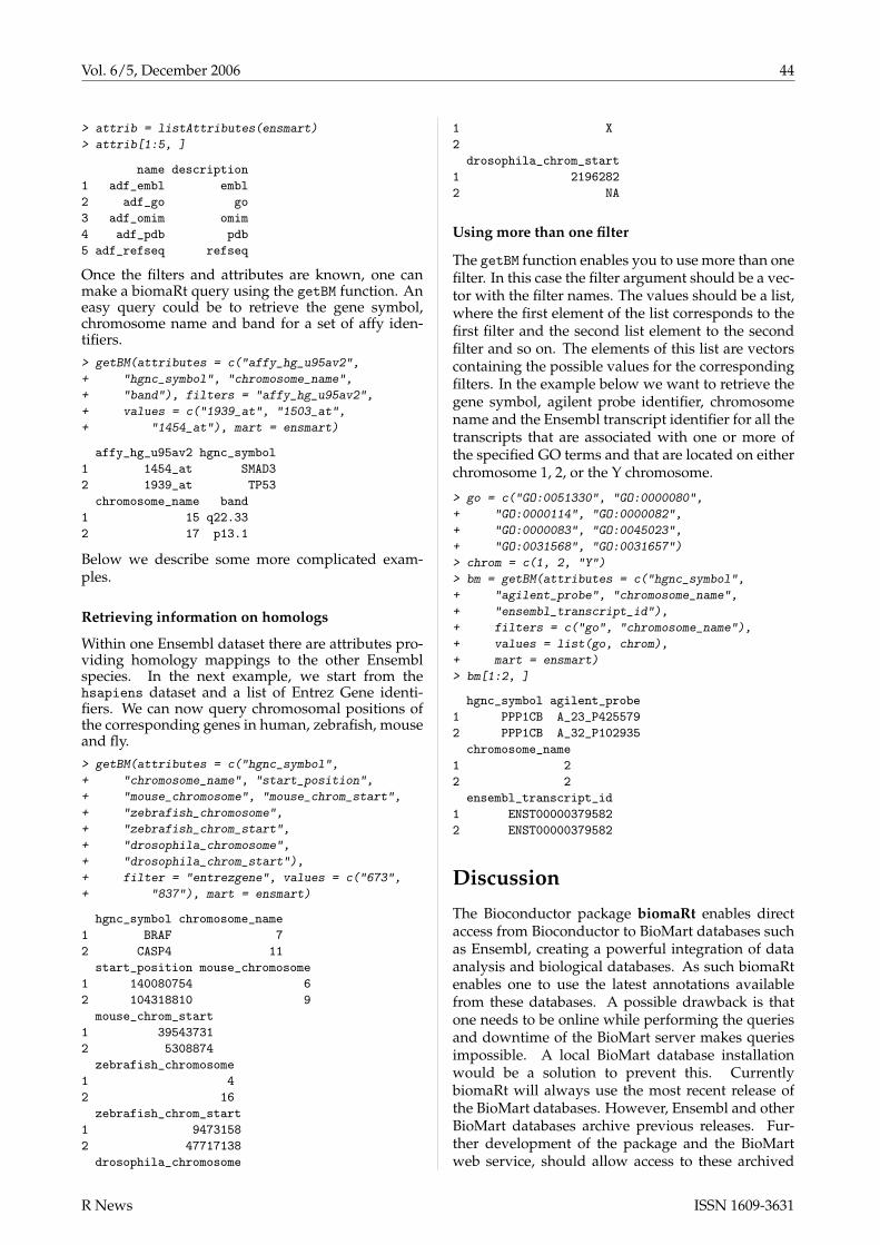
Vol. 6/5, December 2006 44
> attrib = listAttributes(ensmart)
> attrib[1:5, ]
name description
1 adf_embl embl
2 adf_go go
3 adf_omim omim
4 adf_pdb pdb
5 adf_refseq refseq
Once the filters and attributes are known, one canmake a biomaRt query using the getBM function. Aneasy query could be to retrieve the gene symbol,chromosome name and band for a set of affy iden-tifiers.> getBM(attributes = c("affy_hg_u95av2",
+ "hgnc_symbol", "chromosome_name",
+ "band"), filters = "affy_hg_u95av2",
+ values = c("1939_at", "1503_at",
+ "1454_at"), mart = ensmart)
affy_hg_u95av2 hgnc_symbol
1 1454_at SMAD3
2 1939_at TP53
chromosome_name band
1 15 q22.33
2 17 p13.1
Below we describe some more complicated exam-ples.
Retrieving information on homologs
Within one Ensembl dataset there are attributes pro-viding homology mappings to the other Ensemblspecies. In the next example, we start from thehsapiens dataset and a list of Entrez Gene identi-fiers. We can now query chromosomal positions ofthe corresponding genes in human, zebrafish, mouseand fly.> getBM(attributes = c("hgnc_symbol",
+ "chromosome_name", "start_position",
+ "mouse_chromosome", "mouse_chrom_start",
+ "zebrafish_chromosome",
+ "zebrafish_chrom_start",
+ "drosophila_chromosome",
+ "drosophila_chrom_start"),
+ filter = "entrezgene", values = c("673",
+ "837"), mart = ensmart)
hgnc_symbol chromosome_name
1 BRAF 7
2 CASP4 11
start_position mouse_chromosome
1 140080754 6
2 104318810 9
mouse_chrom_start
1 39543731
2 5308874
zebrafish_chromosome
1 4
2 16
zebrafish_chrom_start
1 9473158
2 47717138
drosophila_chromosome
1 X
2
drosophila_chrom_start
1 2196282
2 NA
Using more than one filter
The getBM function enables you to use more than onefilter. In this case the filter argument should be a vec-tor with the filter names. The values should be a list,where the first element of the list corresponds to thefirst filter and the second list element to the secondfilter and so on. The elements of this list are vectorscontaining the possible values for the correspondingfilters. In the example below we want to retrieve thegene symbol, agilent probe identifier, chromosomename and the Ensembl transcript identifier for all thetranscripts that are associated with one or more ofthe specified GO terms and that are located on eitherchromosome 1, 2, or the Y chromosome.
> go = c("GO:0051330", "GO:0000080",
+ "GO:0000114", "GO:0000082",
+ "GO:0000083", "GO:0045023",
+ "GO:0031568", "GO:0031657")
> chrom = c(1, 2, "Y")
> bm = getBM(attributes = c("hgnc_symbol",
+ "agilent_probe", "chromosome_name",
+ "ensembl_transcript_id"),
+ filters = c("go", "chromosome_name"),
+ values = list(go, chrom),
+ mart = ensmart)
> bm[1:2, ]
hgnc_symbol agilent_probe
1 PPP1CB A_23_P425579
2 PPP1CB A_32_P102935
chromosome_name
1 2
2 2
ensembl_transcript_id
1 ENST00000379582
2 ENST00000379582
Discussion
The Bioconductor package biomaRt enables directaccess from Bioconductor to BioMart databases suchas Ensembl, creating a powerful integration of dataanalysis and biological databases. As such biomaRtenables one to use the latest annotations availablefrom these databases. A possible drawback is thatone needs to be online while performing the queriesand downtime of the BioMart server makes queriesimpossible. A local BioMart database installationwould be a solution to prevent this. CurrentlybiomaRt will always use the most recent release ofthe BioMart databases. However, Ensembl and otherBioMart databases archive previous releases. Fur-ther development of the package and the BioMartweb service, should allow access to these archived
R News ISSN 1609-3631

Vol. 6/5, December 2006 45
database releases. The biomaRt package is designedso that new BioMart databases can be automaticallyincluded, once they provide public MySQL access orhave an active BioMart web service. The tight inte-gration of large public databases with data analysisin R makes biomaRt a powerful platform for biolog-ical data integration and data mining.
Bibliography
J. Ashurst, C. Chen, J. Gilbert et al. The VertebrateGenome Annotation (VEGA) database. NucleicAcids Res, 33:D459–465, 2005.
E. Birney, D. Andrews, M. Caccamo et al. Ensembl2006. Nucleic Acids Res, 34:D556–D561, 2006.
S. Durinck, Y. Moreau, A. Kasprzyk et al. Biomart andBioconductor: a powerful link between biologicaldatabases and microarray data analysis. Bioinfor-matics, 21:3439–3440, 2005.
The international hapmap consortium. A haplotypemap of the human genome. Nature, 437:1299–1320,2005.
A. Kasprzyk, D. Keefe, D. Smedley et al. Ensmart: Ageneric system for fast and flexible access to bio-logical data. Genome Res, 14:160–169, 2004.
E. Schwarz, I. Antoshechkin, C. Bastiani et al. Worm-base: better software, richer content. Nucleic AcidsRes, 34:D475–478, 2006.
S. Sherry, M. Ward, M. Kholodov et al. dbSNP: theNCBI database of genetic variation. Nucleic AcidsRes, 29:308–311, 2001.
D. Ware, P. Jaiswal, J. Ni et al. Gramene, a resourcefor comparative grass genomics. Nucleic Acids Res,30(1):103–105, 2002.
C. Wu, R. Apweiler, A. Bairoch et al. The Univer-sal Protein Resource (UniProt): an expanding uni-verse of protein information. Nucleic Acids Res, 34:D187–191, 2006.
Steffen DurinckOncogenomics SectionNIH/NCIGaithersburg MD, [email protected]
Identifying Interesting Genes withsiggenesby Holger Schwender, Andreas Krause and Katja Ickstadt
A common and important task in microarray experi-ments is the identification of genes whose expressionvalues differ substantially between groups or condi-tions. Finding such differentially expressed genes re-quires methods that can deal with multiple testingproblems in which thousands or even tens of thou-sands of hypotheses are tested simultaneously.
Usually, a statistic appropriate for testing if theexpression levels are associated with a covariate ofinterest and the corresponding p-value are computedfor each gene. Afterwards, these raw p-values are ad-justed for multiplicity such that a Type I error rate isstrongly controlled at a pre-specified level of signif-icance. The classical example of such an error rateis the family-wise error rate (FWER), i.e. the proba-bility of at least one false positive. This error rate,however, might be too conservative for a situation inwhich thousands of hypotheses are tested and seve-ral tens of genes should be identified. In the analysisof microarray data, another error rate has hence be-come very popular: The False Discovery Rate (FDR)which is loosely spoken the expected proportion offalse positives among all rejected null hypotheses, i.e.
identified genes.There are, however, other ways to adjust for mul-
tiplicity: For example, QQ plots or the Bayesianframework can be employed for this purpose. If theobserved test statistics are plotted against the valuesof the test statistics that would be expected underthe null hypothesis most of the points will appro-ximately lie on the diagonal. Those points that dif-fer substantially from this line correspond to genesthat are most likely differentially expressed. The Sig-nificance Analysis of Microarrays (SAM) proposedby Tusher et al. (2001) can be used to specify what“differ substantially" means. While Tusher et al.(2001) base their analysis on a moderated t statistic,Schwender et al. (2003) compare this approach witha SAM version based on Wilcoxon rank sums.
Efron et al. (2001) use an empirical Bayes analy-sis (EBAM) to model the distribution of the observedtest statistics as a mixture of two components, onefor the differentially expressed genes and the otherfor the not differentially expressed genes. Follow-ing their analysis, a gene is called differentially ex-pressed if the corresponding posterior probability islarger than 0.9.
Both SAM and EBAM are implemented in the
R News ISSN 1609-3631

Vol. 6/5, December 2006 46
Bioconductor package siggenes. In this article, we,however, will concentrate on SAM. In the following,we briefly describe the SAM procedure, its imple-mentation in siggenes (for more details, see Schwen-der et al., 2003) and the test statistics already avai-lable in this package. Afterwards, we show how youcan write your own function for other testing situa-tions. Finally, we will give an example of how samcan be applied to gene expression data.
Significance Analysis of Microar-rays
In SAM, a statistic d appropriate for testing if thereis an association between the expression levels andthe covariate of interest is computed for each of them genes. These observed test scores are sorted andplotted against the scores expected under the nullhypothesis, where the expected test scores d(i), i =1, . . . , m, are computed as follows: If the null distri-bution is known, then d(i) is the (i− 0.5)/m quantileof this null distribution. Otherwise, d(i) is assessedby
– generating B permutations of the group labels,
– computing the m test statistics and sortingthem for each of the B permutations,
– averaging over the B ith-smallest scores.
Two lines parallel to the diagonal in a distance of ∆
are then drawn into this plot called the SAM plot.Any gene that has a d value
– larger than or equal to the d value of the gene,say dup, that corresponds to the left-most pointon the right side of the origin that lies above theupper ∆ line,
– smaller than or equal to the d value of the gene,say dlow, that corresponds to the right-mostpoint on the left side of the origin that lies be-low the lower ∆ line
is called differentially expressed. Afterwards, theFDR is estimated by
– counting how many of the mB permuted testscores are larger than or equal to dup or smallerthan and equal to dlow, and dividing this num-ber by B,
– dividing this average by the number of identi-fied genes,
– multiplying this ratio by the prior probabilitythat a gene is not differentially expressed (bydefault, sam estimates this probability by theprocedure of Storey and Tibshirani, 2003).
This procedure is repeated for several values of ∆
and the value of ∆ is chosen that provides the bestbalance between the number of identified genes andthe estimated FDR.
The following test statistics can be called in samby setting the argument ‘method’ to
d.stat: Moderated t and F statistics. The “usual” tor F statistics are computed if the fudge factor‘s0’ is set to zero. (The fudge factor is addedto the denominator of the statistics to preventgenes with very low expression levels to be-come differentially expressed. For details, seeTusher et al., 2001).
wilc.stat: Wilcoxon rank sums for one and twoclass analyses.
cat.stat: Pearson’s χ2-statistic for testing categori-cal data such as SNP (Single Nucleotide Poly-morphism) data (Schwender, 2005).
Writing Your Own Test Score Func-tion
It is also possible to write your own function for an-other testing situation and use this function in sam.This function must have as input the two requiredarguments
‘data’: A matrix or data frame containing the data.Each row of this data set should correspond toone of the m variables, i.e. genes, and each col-umn to one of the n observations.
‘cl’: A vector consisting of the class labels of the ob-servations.
The function can also have additional optional argu-ments that can be called in sam.
The output of this function must be a list consi-sting of the following objects
‘d’: A numeric vector containing the test scores of thegenes.
‘d.bar’: A numeric vector of length na.exclude(d)consisting of the sorted test scores expected un-der the null hypothesis.
‘p.value’: A numeric vector of the same length andorder as ‘d’ containing the p-values of thegenes.
‘vec.false’: A numeric vector of the same lengthas ‘d’ consisting of the one-sided numbersof falsely called genes (for more details, seeSchwender et al., 2003, and the help files ofsam).
‘s’: A numeric vector containing the standard errorsof the expression values.
R News ISSN 1609-3631

Vol. 6/5, December 2006 47
‘s0’: A numeric value specifying the fudge factor.
‘mat.samp’: A B× n matrix containing the permutedclass labels.
‘msg’: A character vector containing messages thatare displayed when the SAM specific S4 meth-ods print and summary are called.
‘fold’: A numeric vector containing the foldchanges of the genes. Should be set tonumeric(0) if another analysis than a two-classanalysis is performed.
Assume, e.g., that we would like to perform aSAM analysis with the “usual" t-statistic assumingequal group variances and normality. The code of afunction t.stat for such an analysis is given by
t.stat <- function(data, cl)require(genefilter) ||
stop("genefilter required.")row.out <- rowttests(data, cl)d <- row.out$statisticm <- length(na.exclude(d))d.bar <- qt(((1:m) - 0.5)/m, row.out$df)p.value <- row.out$p.valuevec.false <- m * p.value/2s <- row.out$dm/d# dm: differences in group meansmsg <- paste("SAM Two-Class Analysis",
"Assuming Normality\n\n")list(d=-d, d.bar=d.bar, p.value=p.value,
vec.false=vec.false, s=s, s0=0,mat.samp=matrix(numeric(0)),msg=msg, fold=numeric(0))
Please note that in the output of t.stat ‘d’ is set to-d since in rowttests the mean of group 2 is sub-tracted from the mean of group 1, whereas in sam thedifference is taken the other way around.
Now t.stat can be used in sam by settingmethod=t.stat.
Example: ALL Data
As example we here employ one of the data sets usedin Gentleman et al. (2005). The package ALL contai-ning this data set can be downloaded by
> source("http://www.bioconductor.org/getBioC.R")
> getBioC("ALL")
> library(ALL)> data(ALL)
Even though it is in general not a good idea to fil-ter genes / probe sets prior to a SAM analysis since
SAM assumes that most of the genes are not differen-tially expressed, we here follow the code of Scholtensand von Heydebreck (2005) and filter the genes andselect a subset of the samples.
> library(genefilter)> subALL <- filterALL()
(The code of filterALL can be found in the Ap-pendix.) This leads to an exprSet object containinggene expression data of 2,391 probe sets and 79 sam-ples.
Following Scholtens and von Heydebreck (2005)we would like to identify the probe sets whose ex-pression values differ strongly between the samplesfor which
> mol.biol <- pData(subALL)$mol.biol
is equal to "BCR/ABL" and the samples for whichmol.biol=="NEG". Thus, sam is applied to this dataset by specifying the required arguments ‘data’ and‘cl’, where
‘data’ can either be a matrix, a data frame or anexprSet object containing the gene expressiondata,
‘cl’ is a vector containing the class labels of the sam-ples. If ‘data’ is an exprSet object, then ‘cl’ canalso be a character string naming the column ofpData(data) that contains the class labels.
So
> library(siggenes)> clALL <- ifelse(mol.biol=="BCR/ABL", 0, 1)> dataALL <- exprs(subALL)> out1 <- sam(dataALL, clALL,+ var.equal = TRUE, rand = 123456)
leads to the same results as
> out2 <- sam(subALL, "mol.biol",+ var.equal = TRUE, rand = 123456)
where ‘var.equal’ is set to TRUE since we here wouldlike to assume that the group variances are equal,and ‘rand’ is set to 123456 to make the results of thisanalysis reproducible.
By default, the number of identified genes andthe estimated FDR is computed for ten values of ∆
equidistantly spaced between 0.1 and maxi |d(i) −d(i)|. The output of our SAM analysis is thus givenby
> out1
SAM Analysis for the Two-Class Unpaired CaseAssuming Equal Variances
Delta p0 False Called FDR1 0.1 0.63 1900.61 2075 0.57726
R News ISSN 1609-3631
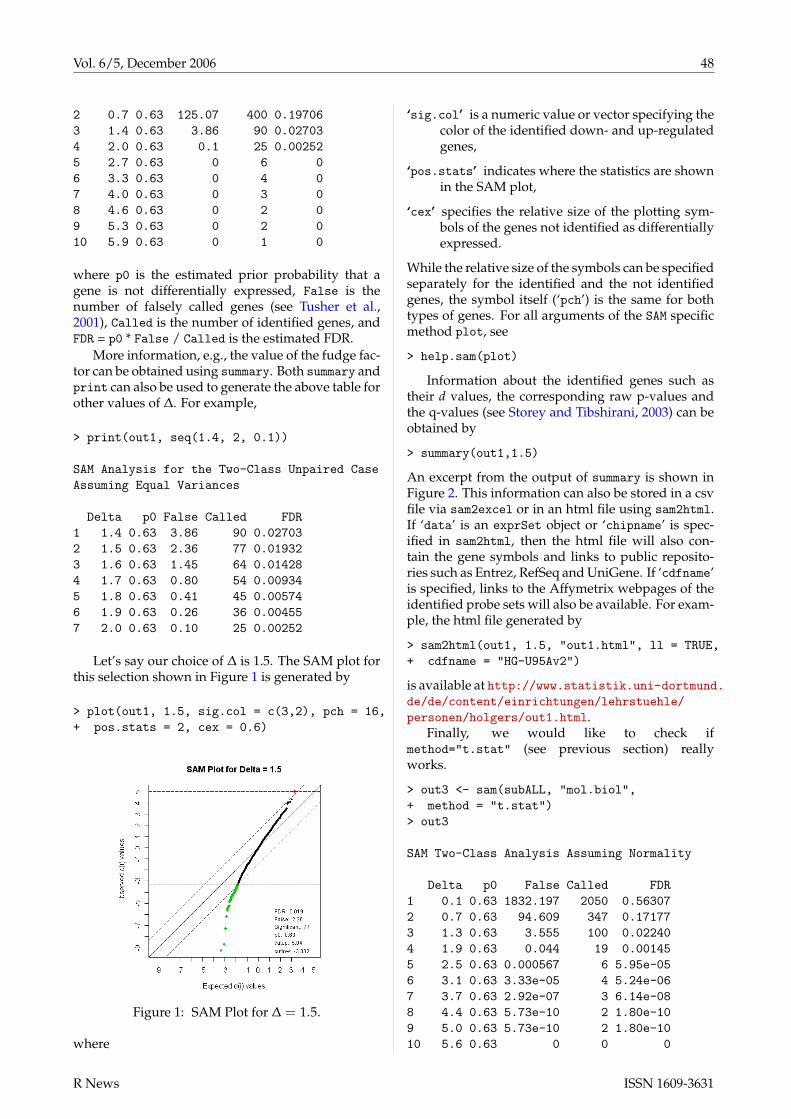
Vol. 6/5, December 2006 48
2 0.7 0.63 125.07 400 0.197063 1.4 0.63 3.86 90 0.027034 2.0 0.63 0.1 25 0.002525 2.7 0.63 0 6 06 3.3 0.63 0 4 07 4.0 0.63 0 3 08 4.6 0.63 0 2 09 5.3 0.63 0 2 010 5.9 0.63 0 1 0
where p0 is the estimated prior probability that agene is not differentially expressed, False is thenumber of falsely called genes (see Tusher et al.,2001), Called is the number of identified genes, andFDR = p0 * False / Called is the estimated FDR.
More information, e.g., the value of the fudge fac-tor can be obtained using summary. Both summary andprint can also be used to generate the above table forother values of ∆. For example,
> print(out1, seq(1.4, 2, 0.1))
SAM Analysis for the Two-Class Unpaired CaseAssuming Equal Variances
Delta p0 False Called FDR1 1.4 0.63 3.86 90 0.027032 1.5 0.63 2.36 77 0.019323 1.6 0.63 1.45 64 0.014284 1.7 0.63 0.80 54 0.009345 1.8 0.63 0.41 45 0.005746 1.9 0.63 0.26 36 0.004557 2.0 0.63 0.10 25 0.00252
Let’s say our choice of ∆ is 1.5. The SAM plot forthis selection shown in Figure 1 is generated by
> plot(out1, 1.5, sig.col = c(3,2), pch = 16,+ pos.stats = 2, cex = 0.6)
Figure 1: SAM Plot for ∆ = 1.5.
where
‘sig.col’ is a numeric value or vector specifying thecolor of the identified down- and up-regulatedgenes,
‘pos.stats’ indicates where the statistics are shownin the SAM plot,
‘cex’ specifies the relative size of the plotting sym-bols of the genes not identified as differentiallyexpressed.
While the relative size of the symbols can be specifiedseparately for the identified and the not identifiedgenes, the symbol itself (‘pch’) is the same for bothtypes of genes. For all arguments of the SAM specificmethod plot, see
> help.sam(plot)
Information about the identified genes such astheir d values, the corresponding raw p-values andthe q-values (see Storey and Tibshirani, 2003) can beobtained by
> summary(out1,1.5)
An excerpt from the output of summary is shown inFigure 2. This information can also be stored in a csvfile via sam2excel or in an html file using sam2html.If ‘data’ is an exprSet object or ‘chipname’ is spec-ified in sam2html, then the html file will also con-tain the gene symbols and links to public reposito-ries such as Entrez, RefSeq and UniGene. If ‘cdfname’is specified, links to the Affymetrix webpages of theidentified probe sets will also be available. For exam-ple, the html file generated by
> sam2html(out1, 1.5, "out1.html", ll = TRUE,+ cdfname = "HG-U95Av2")
is available at http://www.statistik.uni-dortmund.de/de/content/einrichtungen/lehrstuehle/personen/holgers/out1.html.
Finally, we would like to check ifmethod="t.stat" (see previous section) reallyworks.
> out3 <- sam(subALL, "mol.biol",+ method = "t.stat")> out3
SAM Two-Class Analysis Assuming Normality
Delta p0 False Called FDR1 0.1 0.63 1832.197 2050 0.563072 0.7 0.63 94.609 347 0.171773 1.3 0.63 3.555 100 0.022404 1.9 0.63 0.044 19 0.001455 2.5 0.63 0.000567 6 5.95e-056 3.1 0.63 3.33e-05 4 5.24e-067 3.7 0.63 2.92e-07 3 6.14e-088 4.4 0.63 5.73e-10 2 1.80e-109 5.0 0.63 5.73e-10 2 1.80e-1010 5.6 0.63 0 0 0
R News ISSN 1609-3631

Vol. 6/5, December 2006 49
SAM Analysis for the Two-Class Unpaired Case Assuming Equal Variances
s0 = 0
Number of permutations: 100
MEAN number of falsely called genes is computed.
Delta: 1.5
cutlow: -3.332
cutup: 5.04
p0: 0.63
Significant Genes: 77
Falsely Called Genes: 2.36
FDR: 0.0193
Genes called significant (using Delta = 1.5):
Row d.value stdev rawp q.value R.fold Name
1 134 -9.26 0.1188 0 0 0.457 1636_g_at
2 1787 -8.69 0.1327 0 0 0.442 39730_at
3 133 -7.28 0.1652 0 0 0.420 1635_at
4 1890 -6.18 0.2878 0 0 0.429 40202_at
5 1193 -5.65 0.2388 0 0 0.460 37027_at
Figure 2: An excerpt from the output of summary(out1, 1.5).
Since in both analyses we have computed the tstatistic assuming equal group variances, the d va-lues in both analyses should be the same:
> tmp <- sum(round(out1@d, 8) ==+ round(out3@d, 8))> tmp == length(out1@d)[1] TRUE
Summary
The package siggenes contains functions for per-forming both a Significance Analysis of Microarrays(SAM) and an Empirical Bayes Analysis of Microar-rays (EBAM). The function sam provides not only aset of statistics for standard tests such as the t testand F test but also the possibility to use user-writtenfunctions for other testing situations. After identi-fying a list of genes, not only statistics of these genessuch as their test scores and p-values can be obtainedbut also links to public repositories containing bio-logical information about these genes.
The EBAM functions are currently under revi-sion to provide more user-friendly and less memory-consuming versions of these functions having all thefeatures that the SAM functions already have.
This article will be available as vignette insiggenes 1.7.1 and later.
Acknowledgements
The work of Katja Ickstadt and Holger Schwenderhas been supported by the Deutsche Forschungsge-meinschaft, Sonderforschungsbereich 475. The workof Andreas Krause was largely carried out while hewas an employee of Novartis Pharma AG, Basel,Switzerland.
Appendix
filterALL <- function()pdat <- pData(ALL)subset<-intersect(grep("^B",
as.character(pdat$BT)),which(pdat$mol %in% c("BCR/ABL","NEG")))
eset <- ALL[, subset]require(genefilter)f1 <- pOverA(0.25, log2(100))f2 <- function(x) IQR(x) > 0.5selected <- genefilter(eset,
filterfun(f1, f2))esetSub <- eset[selected, ]pdat <- pData(esetSub)esetSub$mol.biol <-
as.character(esetSub$mol.biol)esetSub
R News ISSN 1609-3631

Vol. 6/5, December 2006 50
Bibliography
B. Efron, R. Tibshirani, J. Storey and V. Tusher. Em-pirical Bayes Analysis of a Microarray Experiment.Journal of the American Statistical Association, 96,1151–1160, 2001.
R. Gentleman, V. J. Carey, W. Huber, R. A. Irizarryand S. Dudoit, editors. Bioinformatics and Compu-tational Biology Solutions Using R and Bioconductor.Springer, New York, 2005.
D. Scholtens and A. von Heydebreck. Analysis ofDifferential Gene Expression Studies. In: R. Gen-tleman, V. J. Carey, W. Huber, R. A. Irizarry, S. Du-doit, editors. Bioinformatics and Computational Biol-ogy Solutions Using R and Bioconductor. Springer,New York, 229–248, 2005.
H. Schwender. Modifying Microarray AnalysisMethods for Categorical Data – SAM and PAM forSNPs. In: C. Weihs, W. Gaul, editors. Classification– The Ubiquitous Challenge. Springer, Heidelberg,370–377, 2005.
H. Schwender, A. Krause and K. Ickstadt. Com-parison of the Empirical Bayes and the Signif-
icance Analysis of Microarrays. Technical Re-port, SFB 475, University of Dortmund, Germany,2003. URL http://www.sfb475.uni-dortmund.de/berichte/tr44-03.pdf.
J. D. Storey and R. Tibshirani. Statistical Significancefor Genomewide Studies. Proceedings of the Na-tional Academy of Sciences, 100, 9440–9445, 2003.
V. Tusher, R. Tibshirani and G. Chu. SignificanceAnalysis of Microarrays Applied to the IonizingRadiation Response. Proceedings of the NationalAcademy of Science, 98, 5116–5121, 2001.
Holger Schwender, Katja IckstadtDepartment of Statistics, SFB 475University of Dortmund, [email protected],[email protected]
Andreas KrausePharsight CorporationMountain View, CA, [email protected]
Reverse Engineering Genetic Networksusing the GeneNet Packageby Juliane Schäfer, Rainer Opgen-Rhein, and KorbinianStrimmer
GeneNet is a package for analyzing high-dimensional (time series) data obtained from high-throughput functional genomics assays, such as ex-pression microarrays or metabolic profiling. Specif-ically, GeneNet allows to infer large-scale gene as-sociation networks. These are graphical Gaussianmodels (GGMs) that represent multivariate depen-dencies in biomolecular networks by means of par-tial correlation. Therefore, the output of an analysisconducted by GeneNet is a graph where each genecorresponds to a node and the edges included in thegraph portray direct dependencies between them.
GeneNet implements a specific learning algo-rithm that allows to estimate GGMs from small sam-ple high-dimensional data that is both computation-ally as well as statistically efficient. This approachrelies on analytic shrinkage estimation of covarianceand (partial) correlation matrices and on model se-lection using (local) false discovery rate multiple test-ing. Hence, GeneNet includes a computational algo-rithm that decides which edges are to be included inthe final network, in dependence of the relative val-ues of the pairwise partial correlations.
In a recent comparative survey (Werhli et al.,2006) the GeneNet procedure was found to recoverthe topology of gene regulatory networks with sim-ilar accuracy as computationally much more de-manding methods such as dynamical Bayesian net-works (Friedman, 2004).
We note that the approach implemented inGeneNet should be regarded as an exploratory ap-proach that may help to identify interesting genes(such as “hubs”) or clusters of genes that are func-tionally related or co-regulated, rather than that ityields the precise network of mechanistic interac-tions. Therefore, the resulting network topologiesneed be interpreted and validated in the light of bi-ological background information, ideally accompa-nied by further integrative analysis employing datafrom different levels of the cellular system.
Prerequisites
GeneNet is available from the CRAN repositoryand from the webpage http://strimmerlab.org/software/genenet/. It requires prior installation offour further R packages also found on CRAN: corp-cor, longitudinal, fdrtool, and locfdr (Efron, 2004).
R News ISSN 1609-3631

Vol. 6/5, December 2006 51
For installation of the required packages simplyenter at the R prompt:
> install.packages( c("corpcor","longitudinal", "fdrtool","locfdr", "GeneNet") )
Preparation of Input Data
The input data must be arranged in a matrix wherecolumns correspond to genes and where rows cor-respond to the individual measurements. Note thatthe data must already be properly preprocessed, i.e.in the case of expression data calibrated and normal-ized.
In the following we describe an example for infer-ring the gene association network among 102 genesfrom a microarray data set on the microorganismEscherichia coli with observations at 9 time points(Schmidt-Heck et al., 2004). These example data arepart of GeneNet:
> library("GeneNet")> data(ecoli)> dim(ecoli)[1] 9 102
Shrinkage Estimators of Covari-ance and (Partial) Correlation
The first step in the inference of a graphical Gaussianmodel is the reliable estimation of the partial correla-tion matrix:
> inferred.pcor <- ggm.estimate.pcor(ecoli)> dim(inferred.pcor)[1] 102 102
For this purpose, the function ggm.estimate.pcoroffers an interface to a shrinkage estimator of par-tial correlation implemented in the corpcor pack-age that is statistically efficient and can be used foranalyzing small sample data. By default, the op-tion method="static" is selected, which employs thefunction pcor.shrink. Standard graphical modelingtheory (e.g. Whittaker, 1990) shows that the matrix ofpartial correlations P = (ρi j) is related to the inverseof the covariance matrix Σ. This relationship leads tothe straightforward estimator
ri j = −ωi j/√
ωiiω j j, (1)
whereΩ = (ωi j) = Σ−1. (2)
In Equation 2, it is absolutely crucial that the co-variance is estimated accurately, and that Σ is wellconditioned – otherwise the above formulae will re-sult in a rather poor estimate of partial correlation
(cf. Schäfer and Strimmer, 2005a). For this purpose,the pcor.shrink function uses an analytic shrink-age estimator of the correlation matrix developed inSchäfer and Strimmer (2005b). This linearly com-bines the unrestricted sample correlation with a suit-able correlation target in a weighted average. Se-lecting this target requires some diligence: specifi-cally, we choose to shrink the empirical correlationsR = (ri j) towards the identity matrix, while empir-ical variances are left intact. In this case the analyti-cally determined shrinkage intensity is
λ? =∑i 6= j var(ri j)
∑i 6= j r2i j
. (3)
The resulting shrinkage estimate exhibits a numberof favorable properties. For instance, it is much moreefficient, always positive definite, and well condi-tioned. It is inexpensive to compute and does not re-quire any tuning parameters, as the analytically de-rived optimal shrinkage intensity is estimated fromthe data. Moreover, there are no assumptions aboutthe underlying distributions of the individual esti-mates, except for the existence of the first two mo-ments. These properties carry over to derived quan-tities, such as partial correlations. Furthermore, theresulting estimates are in a form that allows for fastcomputation of their inverse using the Woodburymatrix identity.
Note that the function ggm.estimate.pcor alsoallows the specification of a protect argument, withdefault value protect=0. This imposes limited trans-lation (Efron and Morris, 1972) onto the specifiedfraction of entries of the estimated shrinkage corre-lation matrix, thereby protecting those componentsagainst overshrinkage (see also Opgen-Rhein andStrimmer, 2006c).
Taking Time Series Aspects IntoAccount
Standard Gaussian graphical models assume i.i.d.data whereas in practice many expression data setsresult from time course experiments. One possibilityto generalize the above procedure correspondinglyis to employ dynamic (partial) correlation (Opgen-Rhein and Strimmer, 2006a). This is available in thefunction ggm.estimate.pcor by specifying the op-tion method="dynamic", which in turn relies on thelongitudinal package for computation.
The key difference between dynamical and i.i.d.correlation is that the former takes into account thetime that has elapsed between two subsequent mea-surements. In particular, dynamical correlation al-lows for unequally spaced time points as often en-countered in genomic studies. All small samplelearning procedures (shrinkage) developed for i.i.d.
R News ISSN 1609-3631

Vol. 6/5, December 2006 52
correlation also carry over to dynamical correlation(Opgen-Rhein and Strimmer, 2006b).
Network Search and Model Selec-tion
The second crucial part of gene association networkinference is model selection, i.e. assigning statisticalsignificance to the edges in the GGM network:
> test.results <-ggm.test.edges(inferred.pcor)
> dim(test.results)[1] 5151 6
For this purpose a mixture model,
f (r) = η0 f0(r;κ) + (1− η0) fA(r) , (4)
is fitted to the observed partial correlation coeffi-cients r using the subroutine cor.fit.mixture. f0is the distribution under the null hypothesis of van-ishing partial correlation, η0 is the (unknown) pro-portion of “null edges”, and fA the distribution ofobserved partial correlations assigned to actually ex-isting edges. The latter is assumed to be an arbitrarynonparametric distribution that vanishes for valuesnear zero. This allows for κ, η0, and even fA to bedetermined from the data – see Efron (2004) for analgorithm.
Subsequently, two-sided p-values correspondingto the null hypothesis of zero partial correlation arecomputed for each potential edge using the functioncor0.test. Large-scale simultaneous testing is thenconducted by obtaining q-values via the functionfdr.controlwith the specified value of η0 taken intoaccount. fdr.control uses the algorithms describedin Benjamini and Hochberg (1995) and Storey (2002).An alternative to the q-value approach is to use theempirical Bayes local false discovery rate (fdr) statis-tic (Efron, 2004). This fits naturally with the abovemixture model setup, and in addition takes accountof the dependencies among the estimated partial cor-relation coefficients. The posterior probability that aspecific edge exists given r equals
IP(non-null edge|r) = 1− fdr(r) = 1− η0 f0(r;κ)f (r)
.
(5)Following Efron (2005), we typically consider an
edge to be “significant” if its local fdr is smaller than0.2, or equivalently, if the probability of an edge to be“present” is larger that 0.8:
> signif <- test.results$prob > 0.80> sum(signif)[1] 66> test.results[signif,]
Network Visualization
The network plotting functions in GeneNet rely ex-tensively on the infrastructure offered by the graphand Rgraphviz packages (cf. contribution of SethFalcon in this R News issue).
First, a graph object must be generated containingall significant edges:
> node.labels <- colnames(ecoli)> gr <- ggm.make.graph(
test.results[signif,],node.labels)
> grA graphNEL graph with undirected edgesNumber of Nodes = 102Number of Edges = 66
Subsequently, the resulting object can be inspectedby running the command
> show.edge.weights(gr)
Finally, the gene network topology of the graphicalGaussian model can be visualized using the functionggm.plot.graph:
> ggm.plot.graph(gr,show.edge.labels=FALSE,layoutType="fdp")
The plot resulting from the analysis of the ecoli datais shown in Figure 1. For show.edge.labels=TRUEthe partial correlation coefficients will be printed asedge labels. Note that on some platforms (e.g. Win-dows) the default layoutType="fdp" may not yet beavailable. In this case an alternative variant such as"layoutType=neato" needs to be specified.
Ecoli Gene Association Network
aceB
asnA
atpD
atpG
b1191
b1583
b1963
cchB
cspA
cspG
dnaG
dnaJ
dnaK
eutG fixC
folK
ftsJ
gltA
hupB
ibpB
icdA
lacA
lacY
lacZ
mopB
nmpC
pspA
pspB
sodA
sucA
sucD
tnaA
yaeM
yceP
ycgX
yecO
yedE
yfaD
yfiA
ygcE
yhdM
yheI
yhfV
yjbO
Figure 1: Sparse graphical Gaussian model for 102genes inferred from an E. coli microarray data setwith 9 data points. Full and dotted lines indicate pos-itive and negative partial correlation, respectively.
R News ISSN 1609-3631

Vol. 6/5, December 2006 53
Release History of GeneNet andExample Scripts
The package GeneNet emerged from a reorganiza-tion of the (now obsolete) package GeneTS. Thiswas split into the GeneNet part dealing with genenetwork reconstruction, and the package GeneCyclefor cell cycle and periodicity analysis (Wichert et al.,2004; Ahdesmäki et al., 2005).
On the home page of GeneNet we collect exam-ple scripts in order to guide users of GeneNet whenconducting their own analyses. Currently, this in-cludes the above E. coli data but for instance also anetwork analysis of A. thaliana diurnal cycle genes.We welcome further contributions from the biologi-cal community.
Bibliography
M. Ahdesmäki, H. Lähdesmäki, R. Pearson, H. Hut-tunen, and O. Yli-Harja. Robust detection of peri-odic time series measured from biological systems.BMC Bioinformatics, 6:117, 2005.
Y. Benjamini and Y. Hochberg. Controlling the falsediscovery rate: a practical and powerful approachto multiple testing. J. R. Statist. Soc. B, 57:289–300,1995.
B. Efron. Large-scale simultaneous hypothesis test-ing: the choice of a null hypothesis. J. Am. Statist.Assoc., 99:96–104, 2004.
B. Efron. Local false discovery rates. Preprint, Dept.of Statistics, Stanford University, 2005.
B. Efron and C. N. Morris. Limiting the risk of Bayesand empirical Bayes estimators – part II: The em-pirical Bayes case. J. Am. Statist. Assoc., 67:130–139,1972.
N. Friedman. Inferring cellular networks using prob-abilistic graphical models. Science, 303:799–805,2004.
R. Opgen-Rhein and K. Strimmer. Inferring genedependency networks from genomic longitudinaldata: a functional data approach. REVSTAT, 4:53–65, 2006a.
R. Opgen-Rhein and K. Strimmer. Using regularizeddynamic correlation to infer gene dependency net-works from time-series microarray data. In Pro-ceedings of the 4th International Workshop on Com-putational Systems Biology (WCSB 2006), 12-13 June2006, Tampere, volume 4, pages 73–76, 2006b.
R. Opgen-Rhein and K. Strimmer. Accurate rankingof differentially expressed genes by a distribution-free shrinkage approach. In review.
J. Schäfer and K. Strimmer. An empirical Bayesapproach to inferring large-scale gene associationnetworks. Bioinformatics, 21:754–764, 2005a.
J. Schäfer and K. Strimmer. A shrinkage approach tolarge-scale covariance matrix estimation and im-plications for functional genomics. Statist. Appl.Genet. Mol. Biol., 4(1):Article 32, 2005b.
W. Schmidt-Heck, R. Guthke, S. Toepfer, H. Reis-cher, K. Duerrschmid, and K. Bayer. Reverse en-gineering of the stress response during expressionof a recombinant protein. In Proceedings of the EU-NITE symposium, 10-12 June 2004, Aachen, Germany,pages 407–412, 2004. Verlag Mainz.
J. D. Storey. A direct approach to false discoveryrates. J. R. Statist. Soc. B, 64:479–498, 2002.
A. Werhli, M. Grzegorczyk, and D. Husmeier. Com-parative evaluation of reverse engineering generegulatory networks with relevance networks,graphical Gaussian models and Bayesian net-works. Bioinformatics, 22:2523–2531, 2006.
J. Whittaker. Graphical Models in Applied MultivariateStatistics. Wiley, New York, 1990.
S. Wichert, K. Fokianos, and K. Strimmer. Identify-ing periodically expressed transcripts in microar-ray time series data. Bioinformatics, 20:5–20, 2004.
Juliane Schäfer, ETH Zurich, SwitzerlandRainer Opgen-Rhein, University of Munich, GermanyKorbinian Strimmer, University of Munich, [email protected]@[email protected]
R News ISSN 1609-3631

Vol. 6/5, December 2006 54
A Multivariate Approach to IntegratingDatasets using made4 and ade4by Aedín C. Culhane and Jean Thioulouse
The public microarray repositories, ArrayExpressand the GeneExpression Omnibus (GEO), now con-tain over 100,000 microarray gene expression profiles(Table 1). This is a considerable data resource.
However the average number of arrays perstudy is only between 30 and 40 (Table 1). Giventhat the number of features (genes) on microar-rays now exceeds 50,000, this presents a consid-erable dimensionality problem. Low case to fea-ture ratio is likely to remain an issue, as cost andavailability of biomaterial, such as biopsy tissue,are often limiting. As a result, meta-analysis ormerging data from multiple studies is attractive.
Table 1. Public Microarray Databasesa
Database Arrays StudiesArrayExpressb 44,602 1,487GEOc 87,073 2,353
aStatistics: ArrayExpress (June 2006), GEO (5 July 2006)bhttp://www.ebi.ac.uk/arrayexpress/chttp://www.ncbi.nlm.nih.gov/geo/
Unfortunately, matching of variables (geneprobes) from different microarray technologies ischallenging. Numerous microarray platforms havebeen developed and a number of studies have re-ported disappointingly low correlations betweendifferent technologies. Matching of probes by theirDNA sequence reduces cross-platform inconsis-tency (Carter et al., 2005), and functions to per-form sequence matching are available in the Bio-conductor package matchprobes. EnsEMBL align-ments of DNA probe sequences to the human andother genomes can be retrieved using the pack-age biomaRt. However even the performance ofmatched probes may vary across platforms. Thesedifferences may be due to real biological effectswhere probes on different platforms detect differentsplice variants or homologues of a gene.
A different approach is simply to examine genesor cases with covariant trends across matcheddatasets. We have described the application of co-inertia analysis (CIA) for visualization and analysisof such trends across microarray datasets (Culhaneet al., 2003). Functions to perform these analyses areprovided in the Bioconductor package made4 (Cul-hane et al., 2005). made4 is an extension to ade4(Thioulouse et al., 1997; Chessel et al., 2004), an ex-tensive R package for multivariate analysis of eco-logical data.
Our multivariate approach for cross-platformanalysis of microarray data may be easily applied to
heterogeneous datasets. Increasingly, microarray ex-periments are performed in parallel with proteomics,metabolomics or other high throughput array tech-nologies. Typically the identity of peaks or spotsin proteomics or metabolomics data is unknown.Therefore mapping probes, spots or peaks acrossdatasets is not possible. In analysis of these data, weare simply exploring features (peaks or spots) thathave similar trends across datasets and are correlatedwith a covariate of interest. CIA is suitable for suchan analysis.
We will describe the application of CIA to cross-platform visualization of microarray data and otherfunctions in made4 and ade4 for multivariate analy-sis of biological datasets.
Co-inertia analysis
CIA is a multivariate analysis method that describesthe relationship between two data tables (Dray et al.,2003). It can be used on quantitative, qualitative ordistance matrices. Classical methods, like principalcomponent (PCA) or correspondence analysis (CA),aim at summarizing a table by searching orthogonalaxes on which the projection of the sampling points(cases) have the highest possible variance. This char-acteristic ensures that the associated graphs (factormaps) best represent the initial data (see Figure 1).
To extract information common to two tables,canonical analysis (CANCOR, Gittins, 1985) searchessuccessive pairs of axes (one for each table) with amaximum correlation. The problem is that this anal-ysis may lead to axes with high correlation, but lowpercentages of explained variance. This means that itwill be difficult to give a biological interpretation tothese axes. To overcome this difficulty, CIA searchesfor pairs of axes with maximum covariance (insteadof correlation). This ensures that CIA axes will haveboth a high correlation and also good percentagesof explained variance for each table. Computationsare based on the cross table between the variables ofthe two tables. The importance of each axis is givenby the percentage of total co-inertia, which is similarto the percentage of explained variance for canonicalaxes.
CIA has been successfully applied to visual-ization of cross-platform relationships between mi-croarray datasets (Culhane et al., 2003). CIA is an at-tractive approach as it can be applied to data wherethe number of variables (genes) far exceeds the num-ber of cases, as seen in microarray data. Given datawith such low sample size, CANCOR cannot be used
R News ISSN 1609-3631

Vol. 6/5, December 2006 55
and canonical correspondence analysis (Ter Braak,1986) is reduced to a plain CA (Dray et al., 2003).
Monte-Carlo tests can be used to check the sig-nificance of the relationship between the two tables.The method consists of performing many randompermutation of the cases (arrays), followed by the re-computation of the total co-inertia. By comparing thetotal co-inertia obtained in the normal analysis withthe co-inertias obtained after randomization, one canestimate the probability of the observed relationshipbetween the tables.
PCA or CA of microarray data
PCA and CA are well suited to exploratory analysisof microarray data, and complement popular cluster-ing approaches. While clustering investigates pair-wise distances among objects highlighting fine rela-tionships, PCA and CA examine the variance of thewhole dataset highlighting general trends and gra-dients (reviewed by Brazma and Culhane, 2005). Toperform a PCA or CA on a microarray dataset usingmade4, use the function ord.
To illustrate we apply CA to a microarray geneexpression profiling study of 4 childhood tumors(NB, BL-NHL, EWS, RMS; Khan et al., 2001). A sub-set of these expression data (khan$train, 306 genesx 64 cases), a factor describing the class of each case(khan$train.classes, length=64) and a data frameof gene annotation are available in dataset khan inmade4.
library(made4)data(khan)dataset = khan$trainfac = khan$train.classesgeneSym = khan$annotation$Symbol
results.coa <- ord(dataset, type="coa")par(mfrow= c(1,2))plotarrays(results.coa, classvec=fac)plotgenes(results.coa, genelabels= geneSym)
d = 0.5
EWS
BL−NHL
NB
RMS
Arrays
d = 0.5
LYN
TNNT2 IGF2
AIF1
− MYL4 IGF2
HCLS1 ELF1 HLA−DMA
TNNT1
CDKN3 ISG20 BUB1 MME
COL3A1
PRKAR2B −
FNDC5
MYC
METAP2 GSTM5
TNA CAV1 TLE2
TUBB5
TNFAIP6
MYC
PTPN13
LOXL2
FCGRT OLFM1
GYG2
NFIX FVT1
Genes
Figure 1: CA of a 306 gene subset of Khan dataset(Khan et al., 2001). A) Plot of arrays B) Plot of genes.The further a gene and case are projected in the samedirection from the origin, the stronger association be-tween that gene and case (gene is upregulated in thatarray sample).
Cross-platform analysis using CIA
To perform CIA, objects in the dataset must be"matchable". For example, where multiple studiesare performed on the same samples, CIA can detectco-varying patterns across datasets. If the cases arematched, there is no constraint to match the variables(genes) and the number of variables in each datasetmay differ.
In Example 2, we examine a panel of 60 cell linesfrom the National Cancer Institute (NCI60) that havebeen subjected to gene expression profiling usingAffymetrix (Staunton et al., 2001) and spotted cDNA(Ross et al., 2000) arrays. We apply cia to subsets ofthese 2 datasets which are available in made4.
data(NCI60)names(NCI60)[1] "Ross" "Affy" "classes" "Annot"
fac = NCI60$classes[,2]results.cia = cia(NCI60$Affy, NCI60$Ross)par(mfrow=c(1,2))plotarrays(results.cia, clabel=0)plotarrays(results.cia, clabel=0,
classvec=fac)
In Figure 2, matched cases are joined by a line. Iftwo cases (arrays) have similar profiles, they will beprojected close together. Therefore, the shorter thelength of connecting line the greater the correlation.In Figure 2B, one green case is represented by a longline, indicating a large cross-platform difference be-tween the two expression profiles for this cell line.This may suggest a quality issue in one dataset.
d = 1
60 cases, NCI60 cell lines
d = 1
60 cases, NCI60 cell lines
Figure 2: CIA of NCI60 datasets Affy (closed circles)and Ross (arrows). B). Same as A) but cases are col-ored by class (cancer cell line phenotype). Furtherdetails and interpretation in Culhane (2003).
CIA using "matched" genes
Equally CIA could be performed on variables(genes). Visualization of matched genes across plat-forms is often useful when there is a one:many match
R News ISSN 1609-3631

Vol. 6/5, December 2006 56
of gene probes. On older arrays, a gene was gen-erally only represented by one probe, but on recentmicroarrays a gene maybe represented by 5 or moreprobes (or probesets). In Example 3, we examinemicroarray studies of acute lymphoblastic leukemia(ALL) using older hu6800 (Golub et al., 1999) or morerecent u95av2 (Chiaretti et al., 2004) Affymetrix ar-rays. These datasets are available in Bioconductorpackages golubEsets and ALL.
library(affy)library(ALL)data(ALL)ALL.fac <- substring(ALL$BT,1,1)library(golubEsets)data(Golub_Train)golub <- Golub_Train[,1:27] #ALL datagolub.data <- exprs(golub)#footnote 1golub.data[] <- as.double(golub.data)golub.fac <-golub$T.B.cell
We performed a t-test on the Golub data, usingrowttests in the genefilter package, to select geneswhich were significantly (P<0.001) associated with T-cell or B-cell ALL.
library(genefilter)ttests <- rowttests(golub.data,golub.fac)nsignf <- sum(ttests$p.val < 0.001)topGeneInd <- order(ttests$p.val)[1:nsignf]ttests.signf <-
rownames(golub.data)[topGeneInd]
There were 109 significant gene probes on thehu6800 arrays, which were matched to genes on theu95av2 using biomaRt.
library(biomaRt)mart <- useMart("ensembl", mysql=TRUE)mart <- useDataset("hsapiens_gene_ensembl",
mart)pRef <- getBM(attributes="affy_hg_u95av2",
values=ttests.signf,filters="affy_hugenefl",mart=mart)
anyNA <- function(x) any(is.na(x))pRef <- pRef[!apply(pRef, 1, anyNA), ]dupSet <- function(x, a)
subset(x, a %in% a[duplicated(a)])pMany <- dupSet(pRef, pRef$affy_hugenefl)
Of the 109 hu6800 probesets, 96 mapped to 133u95av2 probesets. Therefore 29 hu6800 probesetsmapped to more than 1 u95av2 probesets. These29:66 "one to many" matches were examined usingcia.
hu6800set <-exprs(golub[pMany$affy_hugenefl, ])
u95av2set <-exprs(ALL[pMany$affy_hg_u95av2, ])
cia.out <- cia(t(hu6800set), t(u95av2set))coordVar1 <- cia.out$coinertia$cocoordVar2 <- cia.out$coinertia$lipar(mfrow=c(2, 2))plotarrays(cia.out, sub="Genes")plotarrays(cia.out, clabel=0,
classvec=pMany$affy_hugenefl)plotarrays(coordVar1, classvec=golub.fac)plotarrays(coordVar2, classvec=ALL.fac)
In Figure 3 we observe that the probesets selectedusing the older hu6800 platform, do appear to dis-criminate B and T cells expression profiles on u95av2arrays. However it appears that only a few geneprobes contribute a significant amount of varianceacross both datasets.
d = 2
Genes
U23852_s_at U23852_s_at.1 U23852_s_at.2
X00437_s_at X00437_s_at.1
U14603_at U14603_at.1
X60992_at X60992_at.1 M26692_s_at M26692_s_at.1 M26692_s_at.2 M13560_s_at
M13560_s_at.1 U18009_at U18009_at.1
U18009_at.2 X95677_at
X95677_at.1 X95677_at.2 X95677_at.3
X73358_s_at
X73358_s_at.1
D11327_s_at D11327_s_at.1 L40386_s_at L40386_s_at.1
X58529_at X58529_at.1
X67098_at X67098_at.1 M13792_at
M13792_at.1 D85131_s_at
D85131_s_at.1
U09578_at
U09578_at.1 U09578_at.2 U18422_at U18422_at.1 S81003_at S81003_at.1
L10717_at L10717_at.1
J03473_at J03473_at.1
U82275_at
U82275_at.1 U79253_at U79253_at.1 U79253_at.2
L01087_at L01087_at.1 X05309_at
X05309_at.1 D13720_s_at D13720_s_at.1
Z30643_at Z30643_at.1
M14676_at M14676_at.1 M14676_at.2
L78833_cds2_at L78833_cds2_at.1
U04241_at
U04241_at.1
Genes, labels hu6800
d = 2
Genes, no labels
d = 0.02
B−cell T−cell
Golub hu6800 arrays
d = 0.05
B−cell T−cell
ALL u95av2 arrays
Figure 3: CIA of a set of genes in golub and ALLdatasets. Projection of probesets A) with and B) with-out hu6800 probe labels, and arrays C),D).
One nice feature of this analysis is that one:manyprobeset matches are clearly visualised. For exam-ple, M13560_s_at, X58529_at, X00437_s_at have 2matches on the hgu95av2 platform. We can see thatonly one M13560_s_at u95av2 probeset matches hasa high loading on the B-cell end of axis 1 (horizontal),indicating that the expression of only one of theseprobesets agrees with the older hu6800 array.
1This processing is only required with golubEset and is not nor-mal processing of ExpressionSet datasets
R News ISSN 1609-3631

Vol. 6/5, December 2006 57
Combining microarray data withgene sequence information
We have also used CIA to integrate microarray datawith counts of motif occurrences in gene promoters,to discover which promoter motifs are most associ-ated with the main patterns of gene expression in adataset (Jeffery et al., 2007). We have also extendedthis approach using between group analysis (Cul-hane et al., 2002), a supervised method where group-ings of arrays or tissues of a-priori interest are con-trasted with the rest. Using between group CIA, weidentify gene motifs (or other gene features) that aremost associated with a gene expression classifier (Jef-fery et al., 2007).
Using ade4 codon usage may be investigated us-ing internal correspondence analysis, a variant ofbetween groups and within groups analyses (Lo-bry and Chessel, 2003). CIA has also been ap-plied to study the relationships between amino-acidphysico-chemical properties and protein composi-tion (Thioulouse and Lobry, 1995). These analysesmaybe facilitated using the seqinr package (Charifet al., 2005). seqinr is an interface between R and theACNUC (Gouy et al., 1985) sequence retrieval sys-tem for nucleotide and protein sequence databasessuch as GenBank, EMBL and SWISS-PROT.
Although we have only described analysis of 2 ta-bles, many other multivariate analysis methods areavailable in ade4, which are easily extended usingthe duality diagram (class dudi) (Chessel et al., 2004).There are several functions for analysis of three-wayor multiple tables (class ktab class, and functionssepan, statis, pta, mcoa, mfa, foucart). Distance ma-trices can be integrated in this framework throughprincipal coordinates analysis (dudi.pco function),and the kdist class in the case of k distance matricesmeasured on the same individuals.
GUIs : ade4TkGUI, Rweb
The made4 package was created to ease the useof multivariate data analysis of microarray gene-expression data. Indeed, it has two main advantages:it is an interface between the ade4 package and Bio-conductor data objects and classes, and it provideswrapper functions to simplify the use of multivari-ate analysis functions implemented in ade4.
Another approach to the simplification is the useof a graphical user interface (GUI). A new package(ade4TkGUI) has been developed using the tcltkpackage to provide a GUI to ade4. This GUI has twospecial features. The first one is a centralized graph-ical display of ade4 dudi objects). The second oneis a dynamic view of factor maps, allowing explo-ration of sample and variable sets by way of zoom-ing, panning, and searching on labels. An Rweb in-terface to seqinr and ade4 multivariate analysis is
also available (http://pbil.univ-lyon1.fr/Rweb/Rweb.general.html).
Summary
The Bioconductor package made4 facilitates multi-variate analysis of microarray data, and builds onextensive experience of multivariate data analysis inecology. Multivariate data analysis methods pro-vide many useful tools to extract meaningful biolog-ical information from these large data sets. Some-times, these methods are overlooked because theyare thought to be complicated and subject to barelymet application hypotheses. This is partly true in theframework of the Gaussian approximation model ofmultivariate analysis. But the geometric model (forexample Le Roux and Rouanet, 2004), and the dual-ity diagram (Holmes, 2006) lift most of these assump-tions.
Bibliography
A. Brazma and A.C. Culhane. Algorithms for geneexpression analysis. In M.J. Dunn, L.B. Jorde, P.F.R.Little, and S. Subramaniam, editors, Encyclopediaof Genetics, Genomics, Proteomics and Bioinformatics.John Wiley and Sons, London, 2005.
S.L. Carter, A.C. Eklund, B.H. Mecham et al. Redefi-nition of affymetrix probe sets by sequence over-lap with cdna microarray probes reduces cross-platform inconsistencies in cancer-associated geneexpression measurements. BMC Bioinformatics, 6:107, 2005.
D. Charif, J. Thioulouse, J.R. Lobry et al. Online syn-onymous codon usage analyses with the ade4 andseqinr packages. Bioinformatics, 21(4):545–7, 2005.
D. Chessel, A. Dufour, and J. Thioulouse. The ADE4package – I: One-table methods. RNews, 4(1):5–10,June 2004.
S. Chiaretti, X. Li, R. Gentleman et al. Gene ex-pression profile of adult T-cell acute lymphocyticleukemia identifies distinct subsets of patientswith different response to therapy and survival.Blood, 103(7):2771–8, 2004.
A.C. Culhane, G. Perrière, E. C. Considine et al.Between-group analysis of microarray data. Bioin-formatics, 18(12):1600–8, 2002.
A.C. Culhane, G. Perrière, and D.G. Higgins. Cross-platform comparison and visualisation of gene ex-pression data using co-inertia analysis. BMC Bioin-formatics, 4:59, 2003.
A.C. Culhane, J. Thioulouse, G. Perrière et al. Made4:an R package for multivariate analysis of gene ex-pression data. Bioinformatics, 21(11):2789–90, 2005.
R News ISSN 1609-3631

Vol. 6/5, December 2006 58
S. Dray, D. Chessel, and J. Thioulouse. Co-inertiaanalysis and the linking of ecological tables. Ecol-ogy, 84:3078–3089, 2003.
R. Gittins. Canonical analysis, a review with applicationsin ecology. Vol.12 of Biomathematics. Springer- Ver-lag, Berlin, 1985.
T.R. Golub, D.K. Slonim, P. Tamayo et al. Molecularclassification of cancer: Class discovery and classprediction by gene expression monitoring. Science,286:531–537, 1999.
M. Gouy, C. Gautier, M. Attimonelli et al. ACNUC–aportable retrieval system for nucleic acid sequencedatabases: logical and physical designs and usage.Comput Appl Biosci, 1(3):167–72, 1985.
S. Holmes. Multivariate analysis: The french way. InD. Nolan and T. Speed, editors, Festschrift for DavidFreedman. IMS, Beachwood, OH, 2006.
I. B. Jeffery, S. F. Madden, P. A. McGettigan et al. In-tegrating transcription factor binding site informa-tion with gene expression datasets. Bioinformatics,23(3):298–305, 2007.
J. Khan, J.S. Wei, M. Ringner et al. Classification anddiagnostic prediction of cancers using gene expres-sion profiling and artificial neural networks. NatMed, 7(6):673–9, 2001.
B. Le Roux and H. Rouanet. Geometric Data Analysis.Kluwer Academic Publishers, Dordrecht, 2004.
J. R. Lobry and D. Chessel. Internal correspondenceanalysis of codon and amino-acid usage in ther-mophilic bacteria. J Appl Genet, 44(2):235–61, 2003.
D.T. Ross, U. Scherf, M.B. Eisen et al. Systematic vari-ation in gene expression patterns in human cancercell lines. Nat Genet, 24(3):227–35, 2000.
J. E. Staunton, D.K. Slonim, H.A. Coller et al.Chemosensitivity prediction by transcriptionalprofiling. Proc Natl Acad Sci USA, 98(19):10787–92,2001.
C. Ter Braak. Canonical correspondence analysis: anew eigenvector technique for multivariate directgradient analysis. Ecology, 69:1167–1179, 1986.
J. Thioulouse and J. Lobry. Co-inertia analysis ofamino-acid physico-chemical properties and pro-tein composition with the ade package. ComputAppl Biosci, 11(3):321–9, 1995.
J. Thioulouse, D. Chessel, S. Dolèdec et al. ADE-4:a multivariate analysis and graphical display soft-ware. Statistics and Computing, 7(1):75–83, 1997.
Aedín C. CulhaneDepartment of Biostatistics and Computational Biology,Dana-Farber Cancer Institute & Department of Biostatis-tics, Harvard School of Public Health, Boston, MA, [email protected]
Jean ThioulouseBiométrie et Biologie Evolutive,CNRS & Université Lyon 1, [email protected]
Using amap and ctc Packages for HugeClusteringby Antoine Lucas and Sylvain Jasson
Introduction
Huge clustering is often required in the field of DNAmicroarray (DeRisi et al., 1997) analysis. A new useof clustering results appears with presentation andexploration software like TreeView (Eisen et al., 1998).
DNA microarray is the most appropriate methodfor high throughput gene studies, allowing expres-sion evaluation of vast gene numbers in differ-ent cells types or conditions. From a technicalpoint of view, microarray analysis first needs im-age processing (for example Imagene (http://www.biodiscovery.com), BZScan (Lopez et al., 2004) orScanAlyze (Eisen et al., 1998)) that gives large tables
of data, followed by statistical processing includingdata normalization.
A main goal of microarray analysis is to detect co-regulated genes presenting similar expression pro-files, which can be achieved by various classificationtechniques. In this area, hierarchical clustering is ofspecial interest as it allows multi-scale cluster visual-ization.
Some R extensions provide efficient clusteringtools (mainly: stats and cluster; Struyf et al., 1997).The packages amap and ctc aim to complete the setof clustering tools for R with:
• Additional features to standard clusteringfunctions.
• A novel PCA method, robust to extreme values.
R News ISSN 1609-3631

Vol. 6/5, December 2006 59
• Fast and optimized and parallelized algo-rithms, which drastically reduce time andmemory requirements so that any computer isable to cluster large data sets.
• The possibility of an external visualization withsoftware such as Treeview (Eisen et al., 1998)and Freeview (http://magix.fri.uni-lj.si/freeview), as shown in Figure 1. This visu-alization software provides convenient clusterexploration and browsing to find relevant in-formation in large cluster trees.
Description
Amap and ctc packages are complementary. Theformer implementa all statistical algorithms and thelatter is used for all interactions with other soft-ware such as the Eisen suite and makes it possi-ble to launch Xcluster (http://genetics.stanford.edu/~sherlock/cluster.html) software within R.
CtcAmapBioconductor
NormalizationAnnotation
R software
Image analyisImageneScanAlyze
Clustering softwareXcluster
Cluster explorationTreeviewFreeview
Bzscan
Figure 1: Amap and ctc usage for microarray analy-sis.
The amap package includes standard hierarchicalclustering and k-means analysis. The novel featuresof amap are a larger selection of distances set likePearson or Spearman (rank-based metric) adapted tomicroarray data and a better hierarchical clusteringimplementation (see the benchmark section).
Clustering can be pre-processed by a principalcomponent analysis, as it projects data into an or-thogonal vector space, which avoids counting corre-lated variables twice. With this analysis, a few ex-treme values may strongly affect the main compo-nents. As the high throughput implies a fully auto-mated data acquisition and therefore outliers gener-ation, we implement robust statistic tools includinga principal component analysis. The main idea ofsuch tools is to minimize the isolated points affectedby lowering their relative weight. This is a recentmethod described by Caussinus et al. (2003).
Figure 2: Results window with Freeview displaying asub-cluster (red part of the tree).
The ctc package has tools to export cluster trees tovisualization software that can explore trees at anyscale to find the suitable magnification dependingon the data specificity and the biological expertise asshown on Figure 2.
The ctc package also makes it convenient to useXcluster software within R. Xcluster performs cluster-ing with a very small memory allocation (it does notcompute the whole distance matrix).
We propose the possibility to import results fromEisen Cluster software to perform post clusteringprocessing with R. Other conversion functions aredesigned to dialog between R and Eisen softwaresuite.
Benchmark
We compare time and memory use with other mainimplementations of standard hierarchical clustering:average link for agglomeration method and Eu-clidean distance (see Figure 3).
It appears that Xcluster has less memory needs(less than 100 MB when others methods use morethan 1.5 GB) since the algorithm used does not com-pute exhaustive distance while agglomerating clus-ters. When using the complete distance matrix,memory use is O(n2) Hierarchical clustering fromamap, stats or cluster packages returns the sametree but cluster includes a post processing that re-works the tree display. The amap implementation ofhcluster or hclusterpar functions are significantlyfaster and allow us to pass the limit of 15000 geneson a recent server in less than half an hour.
R News ISSN 1609-3631

Vol. 6/5, December 2006 60
5000 10000 15000 20000Number of genes
0,01
0,1
1
10
Go
(log
scal
e)
amap/hclusteramap/hclusterpar*ctc/xcluster**cluster/agnesstats/hclust
Memory used
5000 10000 15000 20000Number of genes
0,01
0,10
1,00
10,00
100,00
Hou
rs (l
og sc
ale)
Time used
Figure 3: Benchmark of R package. Sample: simu-lated data, 5000 to 20000 genes under 200 conditions,using average link and Euclidean distance for clus-tering. Computer: dual Xeon processor server, with4 GB RAM and 20 GB swap. System command “time”provides time and memory usage. R version 2.0.1∗ hclusterpar is a parallelized version of hcluster,uses all CPU.∗∗ Xcluster uses a slightly simplified algorithm.
Web application
As many end-users use graphical and intuitive inter-faces, we propose a way to skip the R command lineausterity while using a web interface. We providefiles ‘amap.php’ and ‘ctc.php’ as part of the packages,which produce both form and CGI script, with anystandard apache and php server.
A more sophisticated web application can betested and downloaded at url: http://bioinfo.genopole-toulouse.prd.fr/microarray.
Methods and implementation
The amap core library is implemented in C. Thepackage runs on Linux, Windows, and Mac OS X.Multi-threading and parallelization are disabled onWindows. Both amap and ctc use the free and opensource license GPL.
The amap package is hosted on a source-forge like project manager at http://mulcyber.toulouse.inra.fr/projects/amap by Inra that pro-vides a cvs repository and a bug tracker.
The amap package is also available on CRAN, andthe ctc package is available on Bioconductor.
Acknowledgments
We wish to thank Laurent Gautier and Steffen Möllerfor their contributions.
A. Lucas was supported by the FNS Réseau desGénopôles contract number A1457.
Bibliography
H. Caussinus, M. Fekri, S. Hakam, and A. Ruiz-Gazen. A monitoring display of multivariate out-liers. Computational Statistics & Data Analysis, 44:237–252, October 2003.
J. DeRisi, V. Iyer, and P. Brown. Exploring themetabolic and genetic control of gene expressionon a genomic scale. Science, 278(5338):680–6, 1997.
M. Eisen, P. Spellman, P. Brown, and D. Botstein.Cluster analysis and display of genome-wide ex-pression patterns. Proc. Natl. Acad. Sci. USA, 95:14863–14868, 1998.
F. Lopez, J. Rougemont, B. Loriod et al. Feature ex-traction and signal processing for nylon DNA mi-croarrays. BMC Genomics, 5(1):38, Jun 2004. Eval-uation Studies.
A. Struyf, M. Hubert, and P. Rousseeuw. Integratingrobust clustering techniques in S-PLUS. Compu-tational Statistics and Data Analysis, 26:17–37, Nov1997.
Antoine [email protected]
Sylvain JassonUnité de Biométrie et Intelligence Artificielle, INRA, Cas-tanet Tolosan, [email protected]
Model-based Microarray Image Analysisby Chris Fraley and Adrian E. Raftery
DNA microtechnology has enabled biologists to si-multaneously monitor the expression levels of thou-sands of genes or portions of genes under multi-ple experimental conditions. Many microarray plat-forms exist; what they all have in common is that thegene expression data is obtained via image analysisof the array segments or spots corresponding to the
individual experiments.
A common method for making DNA arrays con-sists of printing the single-stranded DNA represent-ing the genes on a solid substrate using a roboticspotting device. The arrayed DNA spots are thenmixed and hybridized with the cDNA extracted fromthe experimental and control samples. In the two-color array, these samples are treated before hy-bridization with both Cy3 (green) and Cy5 (red)
R News ISSN 1609-3631

Vol. 6/5, December 2006 61
fluorescent dyes. After hybridization, the arraysare scanned at the corresponding wavelengths sepa-rately to obtain the images corresponding to the twochannels. The fluorescence measurements are usedto determine the relative abundance of mRNA orDNA in the samples.
The quantification of the amount of fluorescencefrom the hybridized sample can be affected by a vari-ety of defects that occur during both the manufactur-ing and processing of the arrays, such as perturba-tions of spot positions, irregular spot shapes, holesin spots, unequal distribution of DNA probe withinspots, variable background, and artifacts such asdust and precipitates. Ideally these events should beautomatically recognized in the image analysis, andthe estimated intensities adjusted to take account ofthem.
Li et al. (2005) proposed a method for segmentingmicroarray image blocks, along with a robust model-based method for estimating foreground and back-ground intensities. Peaks and valleys are first locatedin the image signal with a sliding window to auto-matically separate the microarray blocks into regionscontaining the individual spots. Model-based clus-tering (McLachlan and Peel 2000, Fraley and Raftery2002) is then applied to the (univariate) sum of theintensities of the two channels measuring the redand green signals for each spot region to provide aninitial segmentation. Models are fit for up to threegroups (background, foreground, uncertain), and thenumber of groups present is then determined viathe Bayesian Information Criterion (BIC). Wheneverthere is more than one group, the segmentation ispostprocessed in order to remove artifacts. This isdone by reclassifying connected components in thebrightest group that are below a certain threshold insize as unknown. The procedure is described in Fig-ure 1.
1. Automatic gridding.
2. Model-based clustering for ≤ 3 groups.
3. Foreground / background determination:
• If there is more than one group, thresholdconnected components. The foreground istaken to be the group of highest mean in-tensity and the background the group oflowest mean intensity.
• If there is only one group, it is assumedthat no foreground signal is detected.
Figure 1: Basic Procedure for Model-based Segmentationof Microarray Blocks.
This approach combines the strengths ofhistogram-based and spatial methods. It deals effec-
tively with inner holes and artifacts. It also providesa formal inferential basis for deciding when no fore-ground signal is present in a spot. The method hasbeen shown to compare favorably with other meth-ods on experimental microarray data with replicates(Li et al. 2005).
The method is implemented in the Bioconductorpackage spotSegmentation, which consists of twobasic functions:
spotgrid: determines spot locations in blockswithin microarray slides
spotseg: determines foreground and backgroundsignals within individual spots
The spotseg function uses the R package mclust(Fraley and Raftery, 1999, 2003, 2006) for model-based clustering. Other life-sciences applicationsof model-based clustering include grouping coex-pressed genes (Yeung et al. 2001), in vivo MRI of pa-tients with brain tumors (Wehrens et al. 2002), andcontrast-enhanced MRI for breast tumors (Forbeset al. 2004).
The spotSegmentation functions will be illustratedon the first block from the first microarray slideimage from van’t Wout et al. (2003), avail-able as a dataset in Bioconductor under the nameHIVcDNAvantWout03. The encoded image data fromthe two channels for this block are provided asdatasets hiv1raw and hiv2raw, and can be obtainedvia the data command.
> data(hiv1raw)> data(hiv2raw)
The data come from a supplementary websitehttp://ubik.microbiol.washington.edu/HIV/array1/supplemental.htm, where they are encodedfor compact storage. We have chosen to providethese data as given there, so that the following trans-formation is needed in order to extract the intensities:
> dataTrans <- function(x,A=4.7154240E-05)matrix((256*256-1-x)^2*A,nrow=450,ncol=1000)
> hiv1 <- dataTrans(hiv1raw)> hiv2 <- dataTrans(hiv2raw)
Note that this transformation is specific to thisdata; in general stored image data must be con-verted as needed to image intensities. Figure 2shows the image data for the two channels in re-verse gray scale. These plots can be obtained withthe spotSegmentation package using the followingcommands:
> plotBlockImage(sqrt(hiv1))> plotBlockImage(sqrt(hiv2))
R News ISSN 1609-3631

Vol. 6/5, December 2006 62
Figure 2: Reverse gray-scale plots of image intensi-ties from channel 1 (Cy3 green) and channel 2 (Cy5red) of the first block from the first slide of HIV datafrom the Bioconductor dataset HIVcDNAvantWout03.
The function spotgrid can be used to divide themicroarray image block into a grid separating the in-dividual spots.
> hivGrid <- spotgrid( hiv1, hiv2,rows = 12, cols = 32, show = TRUE)
> hivGrid$rowcut
[1] 105 138 163 189 219 244 271 297 326 354379 407 438
$colcut[1] 11 41 66 94 126 163 192 222 250 279
307 338 364 392 419 445 474 501 531 558587 614 641 671 697 727 754 782 808 836862 889 922
Here we have used the knowlege that there are 12rows and 32 columns in a block of the microarrayimage. The show option allows display of the image,shown in the top pannel of Figure 3.The individual spots can now be segmented usingthe function spotseg. The following segments allspots in the block:
hivSeg <- spotseg( hiv1, hiv2,hivGrid$rowcut, hivGrid$colcut)
plot(hivSeg)
The corresponding plot is shown in the bottom pan-nel in Figure 3.
Figure 3: Above: The grid delimiting microar-ray spots determined by function spotgrid, su-perimposed on the sum of the intensities forthe two channels for the Bioconductor datasetHIVcDNAvantWout03. Below: The segmented spotsproduced by spotseg. The color scheme is as fol-lows: black denotes the spots, yellow denotes back-ground, gray denotes pixels of uncertain classifica-tion.
It is possible to process a subset of the regions in thegrid using the arguments R for grid (as opposed topixel) row location of the spot and C for grid columnlocation. The show option in spotseg can be used todisplay details for each spot as it is classified. Whenmore than one spot is processed, the graphics com-mand par(ask = TRUE) should be set so that the dis-plays can be stepped through. The following is anexample of the segmenting and display of an indi-vidual splot.
hivSeg <- spotseg( hiv1, hiv2,hivGrid$rowcut, hivGrid$colcutR = 1, C = 4, show = TRUE)
The resulting display is shown in Figure 4.Mean and median pixel intensities for the fore-ground and background for each channel and eachspot can be recovered through the summary functionapplied to the output of spotseg. For example, thefollowing extracts the summary intensities for thespot shown in Figure 4.
> hivSumry <- summary(hivSeg)
> hivSumry$channel1$foreground$mean[1,4][1] 1475.053
> hivSumry$channel2$background$median[1,4][1] 249.0123
R News ISSN 1609-3631

Vol. 6/5, December 2006 63
Figure 4: spotseg processing of the 1,4 section ofthe gridded HIV image data. Clockwise from topleft: gray-scale image, labeled image after model-based clustering (light yellow: lowest intensity;black: highest intensity), clustered image with con-nected components less than threshold in size la-beled (bright yellow, blue, red denote componentsbelow threshold in size for the light yellow, gray, andblack groups, respectively), final labeling.
Summary
The Bioconductor package spotSegmentation pro-vides functionality for automatic gridding of mi-croarray blocks given the number of rows andcolumns of spots. It also provides functionality fordetermining foreground and background of spots inmicroarray images via model-based clustering. Thisapproach deals effectively with inner holes and arti-facts, as well as providing a formal inferential basisfor deciding when no foreground signal is present ina spot.
Bibliography
F. Forbes, N. Peyrard, C. Fraley, D. Georgian-Smith,D. Goldhaber, and A. Raftery. Model-based region-of-interest selection in dynamic breast MRI. Journalof Computer Assisted Tomography, 30:675–687, 2006.
C. Fraley and A. E. Raftery. MCLUST: Software formodel-based cluster analysis. Journal of Classifica-tion, 16:297–306, 1999.
C. Fraley and A. E. Raftery. Model-based clustering,discriminant analysis and density estimation. Jour-nal of the American Statistical Association, 97:611–631, 2002.
C. Fraley and A. E. Raftery. Enhanced software formodel-based clustering, density estimation, anddiscriminant analysis: MCLUST. Journal of Clas-sification, 20:263–286, 2003.
Q. Li, C. Fraley, R. E. Bumgarner, K. Y. Yeung, andA. E. Raftery. Donuts, scratches, and blanks: Ro-bust model-based segmentation of microarray im-ages. Bioinformatics, 21:2875–2882, 2005.
G. J. McLachlan and D. Peel. Finite Mixture Models.Wiley, 2000.
R. Wehrens, A. W. Simonetti and L. M. .C. Buydens,Mixture modeling of medical magnetic resonancedata. Journal of Chemometrics, 16:274-282, 2002.
A. B. van’t Wout, G. K. Lehrman, S. A. Mikeeva,G. C. O’Keefe, M. G. Katze, R. E. Bumgarner, G. K.Geiss, and J. I. Mullins. Cellular gene expressionupon human immunodeficiency type 1 infection ofCD4(+)-T-cell lines. Journal of Virology, 77(2):1392–1402, January 2003.
K. Y. Yeung, C. Fraley, A. Murua, A. E. Raftery, andW. L. Ruzzo. Model-based clustering and datatransformation for gene expression data. Bioinfor-matics 17, 977–987, 2001.
C. Fraley and A. E. Raftery. MCLUST version 3 for R:Normal mixture modeling and model-based clus-tering. Technical Report No. 504, University ofWashington, September, 2006.
Chris Fraley, Adrian RafteryDepartment of Statistics, Box 354322University of WashingtonSeattle, WA 98195-4322 [email protected]@stat.washington.edu
R News ISSN 1609-3631

Vol. 6/5, December 2006 64
Sample Size Estimation for MicroarrayExperiments Using the ssize Packageby Gregory R. Warnes
Abstract
mRNA Expression Microarray technology is widelyapplied in biomedical and pharmaceutical research.The huge number of mRNA concentrations esti-mated for each sample make it difficult to apply tra-ditional sample size calculation techniques and hasleft most practitioners to rely on rule-of-thumb tech-niques. In this paper, we briefly describe and thendemonstrate a simple method for performing and vi-sualizing sample size calculations for microarray ex-periments as implemented in the ssize R package.
Note
This document is a simplified version of themanuscript
Warnes, G. R., Liu, P. (2006) SampleSize Estimation for Microarray Experi-ments, Technical Report, Department ofBiostatistics and Computational Biology,University of Rochester.
which has been available as a pre-publicationmanuscript since 2004. Please refer to that documentfor a detailed discussion of the sample size estima-tion method and an evaluation of its performance.
Introduction
High-throughput microarray experiments allow themeasurement of expression levels for tens of thou-sands of genes simultaneously. These experimentshave been used in many disciplines of biological re-search, including neuroscience (Mandel et al., 2003),pharmacogenomic research, genetic disease and can-cer diagnosis (Heller, 2002). As a tool for estimat-ing gene expression and single nucleotide polymor-phism (SNP) genotyping, microarrays produce hugeamounts of data which can providing important newinsights.
Microarray experiments are rather costly in termsof materials (RNA sample, reagents, chip, etc), labo-ratory manpower, and data analysis effort. It is crit-ical, therefore, to perform proper experimental de-sign, including sample size estimation, before car-rying out these experiments. Since tens of thou-sands of variables (gene expressions) may be mea-sured on each individual chip, it is essential appro-
priately take into account multiple testing and de-pendency among variables when calculating samplesize.
Method
Overview
Warnes and Liu (2006) provide a simple method forcomputing sample size for microarray experiments,and reports on a series of simulations demonstrat-ing its performance. Surprisingly, despite its sim-plicity, the method performs exceptionally well evenfor data with very high correlation between measure-ments.
The key component of this method is the genera-tion of a cumulative plot of the proportion of genesachieving a desired power as a function of sam-ple size, based on simple gene-by-gene calculations.While this mechanism can be used to select a samplesize numerically based on pre-specified conditions,its real utility is as a visual tool for understanding thetrade off between sample size and power. In our con-sulting work, this latter use as a visual tool has beenexceptionally valuable in helping scientific clients tomake the difficult trade offs between experiment costand statistical power.
Assumptions
In the current implementation, we assume that amicroarray experiment is set up to compare geneexpressions between one treatment group and onecontrol group. We further assume that microarraydata has been normalized and transformed so thatthe data for each gene is sufficiently close to a nor-mal distribution that a standard 2-sample pooled-variance t-test will reliably detect differentially ex-pressed genes. The tested hypothesis for each geneis:
H0 : µT = µC
versusH1 : µT 6= µC
where µT and µC are means of gene expressions fortreatment and control group respectively.
Computations
The proposed procedure to estimate sample size is:
R News ISSN 1609-3631
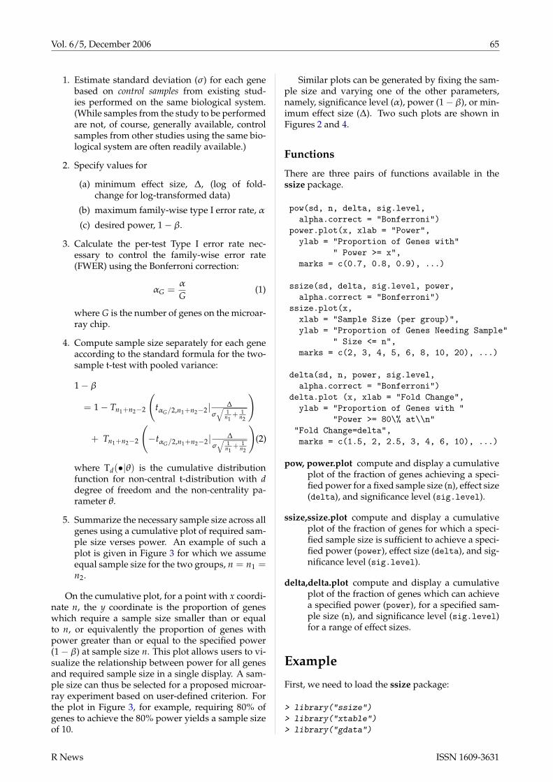
Vol. 6/5, December 2006 65
1. Estimate standard deviation (σ) for each genebased on control samples from existing stud-ies performed on the same biological system.(While samples from the study to be performedare not, of course, generally available, controlsamples from other studies using the same bio-logical system are often readily available.)
2. Specify values for
(a) minimum effect size, ∆, (log of fold-change for log-transformed data)
(b) maximum family-wise type I error rate, α
(c) desired power, 1−β.
3. Calculate the per-test Type I error rate nec-essary to control the family-wise error rate(FWER) using the Bonferroni correction:
αG =α
G(1)
where G is the number of genes on the microar-ray chip.
4. Compute sample size separately for each geneaccording to the standard formula for the two-sample t-test with pooled variance:
1−β
= 1− Tn1+n2−2
(tαG/2,n1+n2−2| ∆
σ√
1n1
+ 1n2
)
+ Tn1+n2−2
(−tαG/2,n1+n2−2| ∆
σ√
1n1
+ 1n2
)(2)
where Td(•|θ) is the cumulative distributionfunction for non-central t-distribution with ddegree of freedom and the non-centrality pa-rameter θ.
5. Summarize the necessary sample size across allgenes using a cumulative plot of required sam-ple size verses power. An example of such aplot is given in Figure 3 for which we assumeequal sample size for the two groups, n = n1 =n2.
On the cumulative plot, for a point with x coordi-nate n, the y coordinate is the proportion of geneswhich require a sample size smaller than or equalto n, or equivalently the proportion of genes withpower greater than or equal to the specified power(1−β) at sample size n. This plot allows users to vi-sualize the relationship between power for all genesand required sample size in a single display. A sam-ple size can thus be selected for a proposed microar-ray experiment based on user-defined criterion. Forthe plot in Figure 3, for example, requiring 80% ofgenes to achieve the 80% power yields a sample sizeof 10.
Similar plots can be generated by fixing the sam-ple size and varying one of the other parameters,namely, significance level (α), power (1−β), or min-imum effect size (∆). Two such plots are shown inFigures 2 and 4.
Functions
There are three pairs of functions available in thessize package.
pow(sd, n, delta, sig.level,alpha.correct = "Bonferroni")
power.plot(x, xlab = "Power",ylab = "Proportion of Genes with"
" Power >= x",marks = c(0.7, 0.8, 0.9), ...)
ssize(sd, delta, sig.level, power,alpha.correct = "Bonferroni")
ssize.plot(x,xlab = "Sample Size (per group)",ylab = "Proportion of Genes Needing Sample"
" Size <= n",marks = c(2, 3, 4, 5, 6, 8, 10, 20), ...)
delta(sd, n, power, sig.level,alpha.correct = "Bonferroni")
delta.plot (x, xlab = "Fold Change",ylab = "Proportion of Genes with "
"Power >= 80\% at\\n""Fold Change=delta",marks = c(1.5, 2, 2.5, 3, 4, 6, 10), ...)
pow, power.plot compute and display a cumulativeplot of the fraction of genes achieving a speci-fied power for a fixed sample size (n), effect size(delta), and significance level (sig.level).
ssize,ssize.plot compute and display a cumulativeplot of the fraction of genes for which a speci-fied sample size is sufficient to achieve a speci-fied power (power), effect size (delta), and sig-nificance level (sig.level).
delta,delta.plot compute and display a cumulativeplot of the fraction of genes which can achievea specified power (power), for a specified sam-ple size (n), and significance level (sig.level)for a range of effect sizes.
Example
First, we need to load the ssize package:
> library("ssize")
> library("xtable")
> library("gdata")
R News ISSN 1609-3631

Vol. 6/5, December 2006 66
The ssize package provides an example data setcontaining gene expression values for smooth mus-cle cells from a control group of untreated healthyvolunteers processed using Affymetrix U95 chipsand normalized per the Robust Multi-array Average(RMA) method of Irizarry et al. (2003).
> data("exp.sd")
> exp.sd <- exp.sd[1:1000]
This data was calculated via:
library("affy")load("probeset_data.Rda")expression.values <- exprs(probeset.data)covariate.data <- pData(probeset.data)controls <- expression.values[,
covariate.data$GROUP=="Control"]exp.sd <- apply(controls, 1, sd)
Let’s see what the distribution looks like:
> par(cex = 2)
> xlab <- c("Standard Deviation",
+ "(for data on the log scale)")
> hist(exp.sd, n = 40, col = "cyan",
+ border = "blue", main = "",
+ xlab = xlab, log = "x")
> dens <- density(exp.sd)
> scaled.y <- dens$y * par("usr")[4]/
+ max(dens$y)
> lines(dens$x, scaled.y,
+ col = "red", lwd = 2)
Standard Deviation(for data on the log scale)
Fre
quen
cy
0.0 0.5 1.0 1.5 2.0
050
100
150
200
250
Figure 1: Standard deviations for of logged exampledata
As is often the case, this distribution is extremelyright skewed, even though the standard deviationswere computed on the log2 scale.
So, now lets see the functions in action. First, de-fine the parameter values we will be investigating:
> n <- 6
> fold.change <- 2
> power <- 0.8
> sig.level <- 0.05
Now, the functions provided by the ssize packagecan be used to address several questions:
1. What is the necessary per-group sample sizefor 80% power when δ = 1.0, and α = 0.05?
> all.size <- ssize(sd = exp.sd,
+ delta = log2(fold.change),
+ sig.level = sig.level,
+ power = power)
> par(cex = 1.3)
> ssize.plot(all.size, lwd = 2,
+ col = "magenta", xlim = c(1,
+ 20))
> xmax <- par("usr")[2] -
+ 1
> ymin <- par("usr")[3] +
+ 0.05
> legend(x = xmax, y = ymin,
+ legend = strsplit(paste("fold change=",
+ fold.change, ",",
+ "alpha=", sig.level,
+ ",", "power=",
+ power, ",", "# genes=",
+ nobs(exp.sd), sep = ""),
+ ",")[[1]], xjust = 1,
+ yjust = 0, cex = 0.9)
> title("Sample Size to Detect 2-Fold Change")
5 10 15 20
Sample Size (per group)
Pro
port
ion
of G
enes
Nee
ding
Sam
ple
Siz
e <
= n
0%
=0
40%
=40
0 8
0%=
800
4
11%=111
5
40%=395
6
60%=602
8
76%=761
10
83%=833
20
95%=946
fold change=2alpha=0.05power=0.8# genes=1000
Sample Size to Detect 2−Fold Change
Figure 2: Sample size required to detect a 2-fold treat-ment effect.
This plot illustrates that a sample size of 10 isrequired to ensure that at least 80% of genes havepower greater than 80%. It also shows that a sample
R News ISSN 1609-3631

Vol. 6/5, December 2006 67
size of 6 is sufficient if only 60% of the genes need toachieve 80% power.
2. What is the power for 6 patients per group withδ = 1.0, and α = 0.05?
> all.power <- pow(sd = exp.sd,
+ n = n, delta = log2(fold.change),
+ sig.level = sig.level)
> power.plot(all.power, lwd = 2,
+ col = "blue")
0.0 0.2 0.4 0.6 0.8 1.0
Power
Pro
port
ion
of G
enes
with
Pow
er >
= x
0%
=0
40%
=40
0 8
0%=
800
0.7
65%=654
0.8
60%=602
0.9
52%=525
n=6fold change=2alpha=0.05# genes=1000
Power to Detect 2−Fold Change
Figure 3: Effect of Sample Size on Power
This plot shows that only 60% of genes achieve at80% power at this sample size and significance level.
3. How large does a fold-change need to be for80% of genes to achieve 80% power for an experi-ment for n = 6 patients per group and α = 0.05?
> all.delta <- delta(sd = exp.sd,
+ power = power, n = n,
+ sig.level = sig.level)
> delta.plot(all.delta, lwd = 2,
+ col = "magenta",
+ xlim = c(1, 10),
+ ylab = paste("Proportion of Genes with ",
+ "Power >= 80% \n",
+ "at Fold Change of delta"))
2 4 6 8 10
Fold Change
Pro
port
ion
of G
enes
with
Pow
er >
= 8
0%
at F
old
Cha
nge
of d
elta
0%
=0
40%
=40
0 8
0%=
800
1.5
16%=156
2
60%=602
2.5
75%=750
3
82%=818
4
90%=897
6
95%=946
10
97%=969
n=6alpha=0.05power=0.8# genes=1000
Fold Change to Achieve 80% Power
Figure 4: Given sample size, this plot allows visual-ization of the fraction of genes achieving the speci-fied power for different fold changes.
This plot shows that for a fold change of 2.0, only60% of genes achieve 80% power, while a fold changeof 3.0 will be detected with 80% power for 80% ofgenes.
Modifications
While the ssize package has been implemented us-ing the simple 2-sample pooled t-test, you can eas-ily modify the code for other circumstances. Simplyreplace the call to power.t.test in each of the func-tions pow,ssize,delta with the appropriate compu-tation for the desired experimental design.
Future Work
Peng Liu is currently developing methods and codefor substituting False Discovery Rate for the Bonfer-roni multiple comparison adjustment.
Contributions
Contributions and discussion are welcome.
Acknowledgment
This work was supported by Pfizer Global Researchand Development.
R News ISSN 1609-3631

Vol. 6/5, December 2006 68
Bibliography
Benjamini, Y. and Hochberg, Y. (1995) Controlling thefalse discovery rate: a practical and powerful ap-proach to multiple testing, Journal of Royal Statisti-cal Society B, 57:1, 289-300.
Dow,G.S. (2003) Effect of sample size and p-valuefiltering techniques on the detection of tran-scriptional changes induced in rat neuroblastoma(NG108) cells by mefloquine, Malaria Journal, 2, 4.
Heller, M. J. (2002) DNA microarray technology: de-vices, systems, and applications, Annual Review inBiomedical Engineering, 4, 129-153.
Hwang,D., Schmitt, W. A., Stephanopoulos, G.,Stephanopoulos, G. (2002) Determination of min-imum sample size and discriminatory expressionpatterns in microarray data, Bioinformatics, 18:9,1184-1193.
Irizarry, R.A., Hobbs, B., Collin, F. et al. (2003) Ex-ploration, normalization, and summaries of highdensity oligonucleotide array probe level data, Bio-statistics, 4:2, 249-264.
Mandel, S., Weinreb, O., Youdim, M. B. H. (2003) Us-ing cDNA microarray to assess Parkinson’s dis-ease models and the effects of neuroprotectivedrugs, TRENDS in Pharmacological Sciences, 24:4,184-191.
Storey, J., (2002) A direct approach to false discoveryrates, Journal of Royal Statistical Society B, 64:3, 479-498.
Warnes, G. R., Liu, P. (2006) Sample Size Estimationfor Microarray Experiments, Technical Report, De-partment of Biostatistics and Computational Biol-ogy, University of Rochester.
Yang, Y. H., Speed, T. Design and analysis of compar-ative microarray experiments, in Statistical analy-sis of gene expression microarray data, Chapman andHall, 51.
Yang, M. C. K., Yang, J. J., McIndoe, R. A., She, J.X. (2003) Microarray experimental design: powerand sample size considerations, Physiological Ge-nomics, 16, 24-28.
Zien, A., Fluck, J., Zimmer, R., Lengauer, T. (2003)Microarrays: how many do you need?, Journal ofComputational Biology, 10:3-4, 653-667.
Gregory WarnesUniversity of RochesterDept. of Biostatistics and Computational BiologyRochester, New York 14642, [email protected]
R News ISSN 1609-3631

Vol. 6/5, December 2006 69
Editor-in-Chief:Paul MurrellDepartment of StatisticsThe University of AucklandPrivate Bag 92019Auckland
Editorial Board:Torsten Hothorn and John Fox.
Editor Programmer’s Niche:Bill Venables
Editor Help Desk:Uwe Ligges
Email of editors and editorial board:firstname.lastname @R-project.org
R News is a publication of the R Foundation for Sta-tistical Computing. Communications regarding thispublication should be addressed to the editors. Allarticles are copyrighted by the respective authors.Please send submissions to regular columns to therespective column editor and all other submissionsto the editor-in-chief or another member of the edi-torial board. More detailed submission instructionscan be found on the R homepage.
R Project Homepage:http://www.R-project.org/
This newsletter is available online athttp://CRAN.R-project.org/doc/Rnews/
R News ISSN 1609-3631