10/2/14  

1  

The Neutral Theory of Molecular Evolution

v Kimura (1968) ²  initially viewed as a challenge to Darwinian

evolution ²  e.g., King & Jukes 1969 Science 164:788-798.

v many genetic polymorphisms have no effect on fitness and are therefore selectively neutral

v neutral polymorphisms are maintained by the combined effects of mutation and drift ² mutations introduce new alleles as others are

lost through drift

Origins of the “Selectionist-Neutralist” Debate

v  the only “mutations” early biologists saw were ones that had phenotypic effects

v  1953 - structure of DNA (Watson & Crick / Franklin) v  1960-70’s - protein electrophoresis

²  revealed allelic diversity for many genes

v  1968 - Motoo Kimura - the neutral theory ²  motivated by allozyme (amino acid) variation

v  discovery of “junk DNA” ²  98.5% of human genome is non-coding

v  DNA sequencing has revealed substantial silent and non-coding variation, suggesting that much genetic variation is selectively neutral (or nearly so!)

10/2/14  

2  

Infinite Alleles/Sites Model

v what is the expected level of genetic diversity (heterozygosity) given mutation and drift in a finite population?

v suppose a gene is 900 base pairs long, coding for 300 amino acids ² there are 4900 = 10542 possible sequences

(sorta…) v thus, we can reasonably assume that each

new mutation generates a unique allele…

Infinite Alleles/Sites Model

v it follows that alleles with the same sequence are identical by descent

v autozygous - a genotype with two alleles that are identical by descent

v allozygous - a genotype with alleles that are not identical by descent (is this possible?) ² arbitrarily declare all alleles unique at t = 0

v autozygous = homozygous under the infinite alleles model ² thus, the level of heterozygosity can be

predicted from the expected level of autozygosity

10/2/14  

3  

Infinite Alleles/Sites Model

v Ft = probability that two randomly chosen alleles are IBD ² same as autozygosity if we randomly choose

alleles to form genotypes

²  in this model, mutations generate new alleles and “erase” IBD

€

Ft =12N"

# $

%

& ' 1−µ( )2 + 1− 1

2N"

# $

%

& ' 1−µ( )2Ft−1

Infinite Alleles Model

v in a random-breeding population of constant size, an equilibrium is reached where the increase in autozygosity (~IBD) due to loss of alleles by drift is exactly countered by the increase in heterozygosity produced by new mutations

v solving for Ft = Ft-1 yields:

€

ˆ F = 11+ 4Nµ

10/2/14  

4  

Infinite Alleles Model

v given the assumption of infinite alleles, any genotype that is not autozygous is heterozygous, so

€

ˆ F = 11+ 4Nµ

=1

1+ 4Neµ=

11+ θ

H =1− F = 4Neµ1+ 4Neµ

=θ1+θ

Neutral Expectations for Genetic Diversity

10/2/14  

5  

v although an ideal population is expected to reach an “equilibrium” value of F, the population is not really at equilibrium, but rather in a “dynamic steady state” because there is a continual turnover of alleles ² the most common allele is periodically

replaced by another, other alleles are lost, and new alleles are produced by mutation

F = 11+ 4Nµ

=11+θ

v DNA sequencing revealed surprisingly high levels of neutral genetic variation

10/2/14  

6  

DNA Sequence-based Measures of Genetic Variation

v S = number of segregating sites v ∏ = average number of pairwise

differences between sequences v ∏ analogous to heterozygosity v can derive theoretical expectations for

both measures for an idealized, random breeding population (and also assuming an “infinite sites” model)…

Segregating sites

v expected number of segregating sites:

v where θ = 4Nµ and k = the number of sequences in the sample

v µ (“mu”) is the per locus mutation rate = mutation rate per site per generation x length of sequence

E S( ) =θ 1+ 12+13+14+...+ 1

k −1"

#$

%

&'

10/2/14  

7  

Coalescent theory often provides “easy” derivations of classical theory

v e.g., number of segregating sites in a sample ²  is a function of the total length (in

generations) of the coalescent tree E(T) times the mutation rate per locus per generation

€

E T( ) = E iTii= 2

k

∑#

$ %

&

' ( = iE Ti( )

i= 2

k

∑ = i 4Ni i −1( )i= 2

k

∑ = 4N 1ii=1

k−1

∑

€

E S( ) = µE T( ) = 4Nµ1ii=1

k−1

∑ = θ1ii=1

k−1

∑

E S( ) = 2 1kk=1

n−1

∑#

$%

&

'(θ2=θ

1kk=1

n−1

∑

Coalescent theory often provides “easy” derivations of classical theory

v e.g., number of segregating sites in a sample ²  is a function of the total length (in

generations) of the coalescent tree E(T) times the mutation rate per locus per generation

E total _ treelength[ ] = kE tk[ ]k=2

n

∑ =2k

k k −1( )k=2

n

∑ = 2 1k −1k=2

n

∑ = 2 1kk=1

n−1

∑

10/2/14  

8  

Average number of pairwise differences

v  in an idealized population, the expected value of ∏ is θ:

v θ can also be estimated from S:

E Π( ) =θ = 4Nµ

θ = E S( ) 1+ 12+13+14+...+ 1

k −1"

#$

%

&'

€

Π =total number of nucleotide mismatchestotal number of pairwise comparisons

θ =16 1+ 12+13+14

!

"#

$

%&= 7.68

E(θ ) =Π =6×6( )+ 4×9( )+ 7×1( )+ 0× 484( )

10#

$%

&

'(= 7.90

10/2/14  

9  

Key point!

v differences in the values for number of segregating sites and average pairwise differences lead to the inference that the gene(s) or the population departs in one or more ways from the ideal “null model” (i.e., constant population size, no selection, etc..)

mtDNA haplotypes for big brown bats (Eptesicus fuscus) east of the Rockies

v θ (∏) = 5.35 v θ (S) = 10.42

10/2/14  

10  

Data versus histories

v generally, the coalescent history of a sample is unknowable

v but, can be crudely approximated by building a gene tree based on DNA sequence data

Rosenberg & Nordborg 2002 Nat Rev Gen

“hanging” mutations on the tree…

10/2/14  

11  

Data versus histories

v generally, the coalescent history of a sample is unknowable

v but, can be crudely approximated by building a gene tree based on DNA sequence data

v genealogical histories estimated with sequence data typically collapse to poorly resolved “networks”

Ornithine decarboxylase intron 6 sequences for mallards, black ducks, and mottled ducks

Harrigan et al. 2008 Mol. Ecol. Resources

10/2/14  

12  

The Ewens Distribution

v beyond F, there is additional “information” available in the number of alleles present and the distribution of allele frequencies ² “allelic configuration” ² or “allele-frequency spectrum”

v Ewens (1972) - expected number of alleles k in a sample of size n, depends on θ

€

E k( ) =1+θ

θ +1+

θθ + 2

+ ...+ θθ + n −1

0

2

4

6

8

10

12

14

16

18

0 5 10 15 20

Exp

ec

ted

num

be

r of u

niq

ue a

llele

s

N (sample size)

0.125

0.25

0.5

1

2

4

8

16

32

€

E k( ) =1+θ

θ +1+

θθ + 2

+ ...+ θθ + n −1

Values of θ = 4Nµ

10/2/14  

13  

The Ewens Sampling Formula

v but there’s more than just k (number of alleles) v the Ewens Distribution specifies the probability

distribution on the set of all partitions of the

integer n ² a.k.a. the “Chinese Restaurant” problem ² broad applicability outside of population

genetics

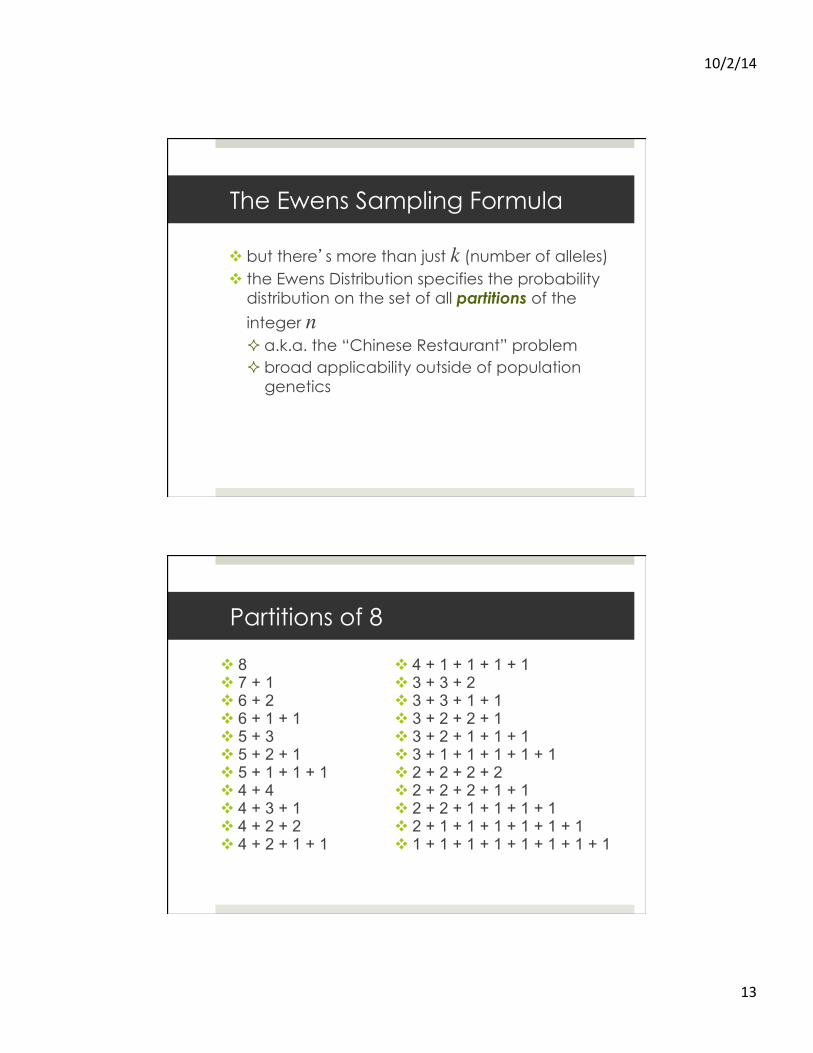
v 8 v 7 + 1 v 6 + 2 v 6 + 1 + 1 v 5 + 3 v 5 + 2 + 1 v 5 + 1 + 1 + 1 v 4 + 4 v 4 + 3 + 1 v 4 + 2 + 2 v 4 + 2 + 1 + 1

Partitions of 8

v 4 + 1 + 1 + 1 + 1 v 3 + 3 + 2 v 3 + 3 + 1 + 1 v 3 + 2 + 2 + 1 v 3 + 2 + 1 + 1 + 1 v 3 + 1 + 1 + 1 + 1 + 1 v 2 + 2 + 2 + 2 v 2 + 2 + 2 + 1 + 1 v 2 + 2 + 1 + 1 + 1 + 1 v 2 + 1 + 1 + 1 + 1 + 1 + 1 v 1 + 1 + 1 + 1 + 1 + 1 + 1 + 1

10/2/14  

14  

Ewens’ Sampling Formula (from Wikipedia!)

v Ewens’ result provided the basis for a formula (Karlin & McGregor, 1972) giving the probability of a given allele frequency configuration (note: this is just one formulation)…

€

Pr a1,...,an{ } =n!

θ θ +1( ) ... θ + n −1( )θ a j

j a j a j!j=1

n

∏

where a1,...,an are counts of the number ofalleles represented one, two,..., n times in

the sample. a1,...,an are nonnegative integers that satisfy : a1 + 2a2 + 3a3 + ...+ nan = n

Karlin & McGregor 1972

€

Pr θ ; n1, n2,..., nk( ) =r!

n1n2 ... nk1

α1!α2!...α p!θ k

Lr θ( )where Lr θ( ) = θ θ +1( ) θ +1( ) ... θ + r −1( )

v this equation works too…

10/2/14  

15  

10/2/14  

16  

Ewens’ Sampling Formula

v key point: the Ewens distribution provides a basis for testing observed data against the neutral model

Ewens’ Sampling Formula

v key point: the Ewens distribution provides a basis for testing observed data against the neutral model

v and if the data fit neutral expectations, they can be used to estimate demographic and historical parameters

10/2/14  

17  

Site Frequency Spectrum

v applicable to DNA sequence data v what is the distribution of frequencies for

individual mutations (SNPs)

v number of derived “singletons” = θ v why?

²  length of “external branches” = 4N generations

²  (note: t = 2 in Nielsen & Slatkin)

v  frequency distribution for derived mutations

E fj!" #$=1/ j

1kk−1

n−1

∑, for j = 1, 2, ... , n-1

Neutral Expectations with…

v  ...constant population size and mutation

E S( ) =θ 1+ 12+13+14+...+ 1

k −1"

#$

%

&'

E Π( ) =θ = 4Nµ

H =θ1+θ

€

E k( ) =1+θ

θ +1+

θθ + 2

+ ...+ θθ + n −1

Pr a1,...,an{ }=n!

θ θ +1( ) ... θ + n−1( )θ aj

jaj aj !j=1

n

∏

nucleotide diversity (infinite sites) # segregating sites (infinite sites) heterozygosity (infinite alleles) # unique alleles (infinite alleles) allele frequency distribution (infinite alleles) site frequency distribution (infinite sites)

E fj!" #$=1/ j

1kk−1

n−1

∑, for j = 1, 2, ... , n-1

10/2/14  

18  

The coalescent with population growth

v coalescent trees are expected to be sparse (few lineages) near the root for populations of constant size

v in a growing or shrinking population, the distribution of coalescence times differs from expectations for the ideal population

v expanding populations have more nodes closer to the root of the tree ² takes longer for alleles to “find each other” in

a growing population

constant

10/2/14  

19  

growing

declining

10/2/14  

20  

constant growing declining

So, what’s the point?

v coalescent modeling ² simulate genealogies under a given set of

population parameters ² “hang” random mutations on those trees in

equal number (or at the same rate) as in the observed data

² evaluate whether the observed data could have been produced by a random coalescent process (the null hypothesis)