The NEURON Simulation Environment · and exploring the operation of brain mechanisms in a ... “wet lab” experiment. ... Using the NEURON Simulation Environment © 10/97 MLH and

Short course: Using the NEURON Simulation Environment © 10/97 MLH and NTC all rights reserved

The NEURON Simulation Environment

M.L. Hines1, 3 and N.T. Carnevale2, 3

Departments of 1Computer Science and 2Psychology

and 3Neuroengineering and Neuroscience Center

Yale University

[email protected]

[email protected]

an extended preprint of

Hines, M.L. and Carnevale, N.T.:

The NEURON Simulation Environment

Neural Computation 9:1179-1209, 1997.

2 The NEURON Simulation Environment


CONTENTS

1. INTRODUCTION ....................................................................................................................................... 31.1 The problem domain..........................................................................................................................................31.2 Experimental advances and quantitative modeling.........................................................................................3

2. OVERVIEW OF NEURON ........................................................................................................................ 4

3. MATHEMATICAL BASIS............................................................................................................................ 43.1 The cable equation .............................................................................................................................................53.2 Spatial discretization in a biological context: sections and segments.............................................................63.3 Integration methods...........................................................................................................................................8

3.3.1 The forward Euler method: simple, unstable, inaccurate .......................................................................83.3.2 Numerical stability......................................................................................................................................93.3.3 The backward Euler method: inaccurate but stable..............................................................................103.3.4 Error ..........................................................................................................................................................113.3.5 Crank-Nicholson Method: stable and more accurate ............................................................................123.3.6 The integration methods used in NEURON............................................................................................133.3.7 Efficiency ...................................................................................................................................................13

4. THE NEURON SIMULATION ENVIRONMENT....................................................................................... 154.1 The hoc interpreter ..........................................................................................................................................154.2 A specific example............................................................................................................................................15

4.2.1 First step: establish model topology .......................................................................................................164.2.2 Second step: assign anatomical and biophysical properties ..................................................................164.2.3 Third step: attach stimulating electrodes................................................................................................174.2.4 Fourth step: control simulation time course ...........................................................................................17

4.3 Section variables ..............................................................................................................................................174.4 Range variables ................................................................................................................................................184.5 Specifying geometry: stylized vs. 3-D .............................................................................................................194.6 Density mechanisms and point processes.......................................................................................................204.7 Graphical interface ..........................................................................................................................................224.8 Object-oriented syntax ....................................................................................................................................22

4.8.1 Neurons......................................................................................................................................................224.8.2 Networks....................................................................................................................................................23

5. SUMMARY............................................................................................................................................... 24

REFERENCES .............................................................................................................................................. 24

APPENDIX 1. LISTING OF hoc CODE FOR THE MODEL IN SECTION 4.2................................................... 26

The NEURON Simulation Environment 3


1. INTRODUCTION

NEURON (Hines 1984; 1989; 1993; 1994)provides a powerful and flexible environment forimplementing biologically realistic models of electricaland chemical signaling in neurons and networks ofneurons. This article describes the concepts andstrategies that have guided the design andimplementation of this simulator, with emphasis onthose features that are particularly relevant to its mostefficient use.

1.1 The problem domain

Information processing in the brain results from thespread and interaction of electrical and chemicalsignals within and among neurons. This involvesnonlinear mechanisms that span a wide range of spatialand temporal scales (Carnevale and Rosenthal 1992)and are constrained to operate within the intricateanatomy of neurons and their interconnections.Consequently the equations that describe brainmechanisms generally do not have analytical solutions,and intuition is not a reliable guide to understanding theworking of the cells and circuits of the brain.Furthermore, these nonlinearities and spatiotemporalcomplexities are quite unlike those that are encounteredin most nonbiological systems, so the utility of manyquantitative and qualitative modeling tools that weredeveloped without taking these features intoconsideration is severely limited.

NEURON is designed to address these problemsby enabling both the convenient creation of biologicallyrealistic quantitative models of brain mechanisms andthe efficient simulation of the operation of thesemechanisms. In this context the term “biologicalrealism” does not mean “infinitely detailed.” Instead itmeans that the choice of which details to include in themodel and which to omit are at the discretion of theinvestigator who constructs the model, and not forcedby the simulation program.

To the experimentalist NEURON offers a tool forcross-validating data, estimating experimentallyinaccessible parameters, and deciding whether knownfacts account for experimental observations. To thetheoretician it is a means for testing hypotheses anddetermining the smallest subset of anatomical andbiophysical properties that is necessary and sufficient toaccount for particular phenomena. To the student in alaboratory course it provides a vehicle for illustratingand exploring the operation of brain mechanisms in a

simplified form that is more robust than the typical“wet lab” experiment. For experimentalist, theoretician,and student alike, a powerful simulation tool such asNEURON can be an indispensable aid to developingthe insight and intuition that are needed if one is todiscover the order hidden within the intricacy ofbiological phenomena, the order that transcends thecomplexity of accident and evolution.

1.2 Experimental advances andquantitative modeling

Experimental advances drive and supportquantitative modeling. Over the past two decades thefield of neuroscience has seen striking developments inexperimental techniques that include• high-quality electrical recording from neurons in

vitro and in vivo using patch clamp• multiple impalements of visually identified cells• simultaneous intracellular recording from paired

pre- and postsynaptic neurons• simultaneous measurement of electrical and

chemical signals• multisite electrical and optical recording• quantitative analysis of anatomical and biophysical

properties from the same neuron• photolesioning of cells• photorelease of caged compounds for spatially

precise chemical stimulation• new drugs such as channel blockers and receptor

agonists and antagonists• genetic engineering of ion channels and receptors• analysis of mRNA and biophysical properties from

the same neuron• “knockout” mutationsThese and other advances are responsible forimpressive progress in the definition of the molecularbiology and biophysics of receptors and channels, theconstruction of libraries of identified neurons andneuronal classes that have been characterizedanatomically, pharmacologically, and biophysically,and the analysis of neuronal circuits involved inperception, learning, and sensorimotor integration.

The result is a data avalanche that catalyzes theformulation of new hypotheses of brain function, whileat the same time serving as the empirical basis for thebiologically realistic quantitative models that must beused to test these hypotheses. Some examples from thelarge list of topics that have been investigated throughthe use of such models include



• the cellular mechanisms that generate and regulatechemical and electrical signals (Destexhe et al.1996; Jaffe et al. 1994)

• drug effects on neuronal function (Lytton andSejnowski 1992)

• presynaptic (Lindgren and Moore 1989) andpostsynaptic (Destexhe and Sejnowski 1995;Traynelis et al. 1993) mechanisms underlyingcommunication between neurons

• integration of synaptic inputs (Bernander et al.1991; Cauller and Connors 1992)

• action potential initiation and conduction (Häusseret al. 1995; Hines and Shrager 1991; Mainen et al.1995)

• cellular mechanisms of learning (Brown et al.1992; Tsai et al. 1994a)

• cellular oscillations (Destexhe et al. 1993a; Lyttonet al. 1996)

• thalamic networks (Destexhe et al. 1993b;Destexhe et al. 1994)

• neural information encoding (Hsu et al. 1993;Mainen and Sejnowski 1995; Softky 1994)

2. OVERVIEW OF NEURONNEURON is intended to be a flexible framework

for handling problems in which membrane propertiesare spatially inhomogeneous and where membranecurrents are complex. Since it was designed specificallyto simulate the equations that describe nerve cells,NEURON has three important advantages over generalpurpose simulation programs. First, the user is notrequired to translate the problem into another domain,but instead is able to deal directly with concepts thatare familiar at the neuroscience level. Second,NEURON contains functions that are tailoredspecifically for controlling the simulation and graphingthe results of real neurophysiological problems. Third,its computational engine is particularly efficientbecause of the use of special methods that takeadvantage of the structure of nerve equations (Hines1984; Mascagni 1989).

However, the general domain of nerve simulationis still too large for any single program to dealoptimally with every problem. In practice, eachprogram has its origin in a focused attempt to solve arestricted class of problems. Both speed of simulationand the ability of the user to maintain conceptualcontrol degrade when any program is applied toproblems outside the class for which it is best suited.

NEURON is computationally most efficient forproblems that range from parts of single cells to smallnumbers of cells in which cable properties play acrucial role. In terms of conceptual control, it is bestsuited to tree-shaped structures in which the membranechannel parameters are approximated by piecewiselinear functions of position. Two classes of problemsfor which it is particularly useful are those in which it isimportant to calculate ionic concentrations, and thosewhere one needs to compute the extracellular potentialjust next to the nerve membrane. It is especiallycapable for investigating new kinds of membranechannels since they are described in a high levellanguage (NMODL (Moore and Hines 1996)) whichallows the expression of models in terms of kineticschemes or sets of simultaneous differential andalgebraic equations. To maintain efficiency, userdefined mechanisms in NMODL are automaticallytranslated into C, compiled, and linked into the rest ofNEURON.

The flexibility of NEURON comes from a built-inobject oriented interpreter which is used to define themorphology and membrane properties of neurons,control the simulation, and establish the appearance ofa graphical interface. The default graphical interface issuitable for exploratory simulations involving thesetting of parameters, control of voltage and currentstimuli, and graphing variables as a function of timeand position.

Simulation speed is excellent since membranevoltage is computed by an implicit integration methodoptimized for branched structures (Hines 1984). Theperformance of NEURON degrades very slowly withincreased complexity of morphology and membranemechanisms, and it has been applied to very largenetwork models (104 cells with 6 compartments each,total of 106 synapses in the net [T. Sejnowski, personalcommunication]).

3. MATHEMATICAL BASIS

Strategies for numerical solution of the equationsthat describe chemical and electrical signaling inneurons have been discussed in many places. Elsewherewe have briefly presented an intuitive rationale for themost commonly used methods (Hines and Carnevale1995). Here we start from this base and proceed toaddress those aspects which are most pertinent to thedesign and application of NEURON.



3.1 The cable equation

The application of cable theory to the study ofelectrical signaling in neurons has a long history, whichis briefly summarized elsewhere (Rall 1989). The basiccomputational task is to numerically solve the cableequation

∂∂

∂∂

V

tI V t

V

x+ =,b g

2

2(1)

which describes the relationship between current andvoltage in a one-dimensional cable. The branchedarchitecture typical of most neurons is incorporated bycombining equations of this form with appropriateboundary conditions.

i a

i a

i m

i ai m

i a

i m

Figure 3.1. The net current entering a region mustequal zero.

Spatial discretization of this partial differentialequation is equivalent to reducing the spatiallydistributed neuron to a set of connected compartments.The earliest example of a multicompartmental approachto the analysis of dendritic electrotonus was providedby Rall (1964).

Spatial discretization produces a family of ordinarydifferential equations of the form

cdv

dti

v v

rjj

ionk j

jkkj

+ =−

∑ (2)

Equation 2 is a statement of Kirchhoff’s current law,which asserts that net transmembrane current leavingthe jth compartment must equal the sum of axialcurrents entering this compartment from all sources(Fig. 3.1). The left hand side of this equation is the totalmembrane current, which is the sum of capacitive andionic components. The capacitive component is

c dv dtj j , where cj is the membrane capacitance of the

compartment. The ionic component iion j includes all

currents through ionic channel conductances. The righthand side of Eq. 2 is the sum of axial currents that enterthis compartment from its adjacent neighbors. Currentsinjected through a microelectrode would be added tothe right hand side. The sign conventions for currentare: outward transmembrane current is positive; axialcurrent flow into a region is positive; positive injectedcurrent drives vj in a positive direction.

Equation 2 involves two approximations. First,axial current is specified in terms of the voltage dropbetween the centers of adjacent compartments. Thesecond approximation is that spatially varyingmembrane current is represented by its value at thecenter of each compartment. This is much less drasticthan the often heard statement that a compartment isassumed to be “isopotential.” It is far better to picturethe approximation in terms of voltage varying linearlybetween the centers of adjacent compartments. Indeed,the linear variation in voltage is implicit in the usualdescription of a cable in terms of discrete electricalequivalent circuits.

If the compartments are of equal size, it is easy touse Taylor's series to show that both of theseapproximations have errors proportional to the squareof compartment length. Thus replacing the secondpartial derivative by its central differenceapproximation introduces errors proportional to ∆x2,and doubling the number of compartments reduces theerror by a factor of four.

It is often not convenient for the size of allcompartments to be equal. Unequal compartment sizemight be expected to yield simulations that are onlyfirst order accurate. However, comparison ofsimulations in which unequal compartments are halvedor quartered in size generally reveals a second-orderreduction of error. A rough rule of thumb is thatsimulation error is proportional to the square of the sizeof the largest compartment.

The first of two special cases of Eq. 2 that we wishto discuss allows us to recover the usual parabolicdifferential form of the cable equation. Consider theinterior of an unbranched cable with constant diameter.The axial current consists of two terms involvingcompartments with the natural indices j–1 and j+1 , i.e.

cdv

dti

v v

r

v v

rjj

ionj j

j j

j j

j jj

+ =−

+−−

−

+

+

1

1

1

1, ,



If the compartments have the same length ∆x anddiameter d, then the capacitance of a compartment isCm π d ∆x and the axial resistance is Ra ∆x / π (d/2)2. Cm

is called the specific capacitance of the membrane,which is generally taken to be 1 µf / cm2. Ra is the axialresistivity, which has different reported values fordifferent cell classes (e.g. 35.4 Ω cm for squid axon).Eq. 2 then becomes

Cdv

dti

d

R

v v v

xm

jj

a

j j j+ =− ++ −

4

21 12∆

where we have replaced the total ionic current iion j

with the current density i j . The right hand term, as

∆x → 0, is just ∂ ∂2 2V x at the location of the nowinfinitesimal compartment j.

The second special case of Eq. 2 allows us torecover the boundary condition. This is an importantexercise since naive discretizations at the ends of thecable have destroyed the second order accuracy ofmany simulations. Nerve boundary conditions are thatno axial current flows at the end of the cable, i.e. theend is sealed. This is implicit in Eq. 2, where the righthand side consists only of the single term

v v rj j j j− −−1 1d i , when compartment j lies at the end of

an unbranched cable.

3.2 Spatial discretization in abiological context: sectionsand segments

Every nerve simulation program solves for thelongitudinal spread of voltage and current byapproximating the cable equation as a series ofcompartments connected by resistors (Fig. 3.4 andEq. 2). The sum of all the compartment areas is thetotal membrane area of the whole nerve. Unfortunately,it is usually not clear at the outset how manycompartments should be used. Both the accuracy of theapproximation and the computation time increase as thenumber of compartments used to represent the cableincreases. When the cable is “short,” a singlecompartment can be made to adequately represent theentire cable. For long cables or highly branchedstructures, it may be necessary to use a large number ofcompartments.

This raises the question of how best to manage allthe parameters that exist within these compartments.

Consider membrane capacitance, which has a differentvalue in each compartment. Rather than specify thecapacitance of each compartment individually, it isbetter to deal in terms of a single specific membranecapacitance which is constant over the entire cell andhave the program compute the values of the individualcapacitances from the areas of the compartments. Otherparameters such as diameter or channel density mayvary widely over short distances, so the graininess oftheir representation may have little to do withnumerically adequate compartmentalization.

Although NEURON is a compartmental modelingprogram, the specification of biological properties(neuron shape and physiology) has been separated fromthe numerical issue of compartment size. What makesthis possible is the notion of a section, which is acontinuous length of unbranched cable. Although eachsection is ultimately discretized into compartments,values that can vary with position along the length of asection are specified in terms of a continuous parameterthat ranges from 0 to 1 (normalized distance). In thisway, section properties are discussed without regard tothe number of segments used to represent it. Thismakes it easy to trade off between accuracy and speed,and enables convenient verification of the numericalcorrectness of simulations.

Sections are connected together to form any kindof branched tree structure. Fig. 3.2 illustrates howsections are used to represent biologically significantanatomical features. The top of this figure is a cartoonof a neuron with a soma that gives rise to a brancheddendritic tree and an axon hillock connected to amyelinated axon. Each biologically significantcomponent of this cell has its counterpart in one of thesections of the NEURON model, as shown in thebottom of Fig. 3.2: the cell body (Soma), axon hillock(AH), myelinated internodes (Ii), nodes of Ranvier (Ni),and dendrites (Di). Sections allow this kind offunctional/anatomical parcellation of the cell to remainforemost in the mind of the person who constructs anduses a NEURON model.

To accommodate requirements for numericalaccuracy, NEURON represents each section by one ormore segments of equal length (Figs. 3.3 and 3.4). Thenumber of segments is specified by the parameternseg, which can have a different value for eachsection.

At the center of each segment is a node, thelocation where the internal voltage of the segment isdefined. The transmembrane currents over the entiresurface area of a segment are associated with its node.



The nodes of adjacent segments are connected byresistors.

Figure 3.2. Top: cartoon of a neuron indicating theapproximate boundaries between biologicallysignificant structures. The left hand side of the cellbody (Soma) is attached to an axon hillock (AH)that drives a myelinated axon (myelinatedinternodes Ii alternating with nodes of Ranvier Ni).From the right hand side of the cell body originatesa branched dendritic tree (Di). Bottom: howsections would be employed in a NEURON modelto represent these structures.

It is crucial to realize that the location of thesecond order correct voltage is not at the edge of asegment but rather at its center, i.e. at its node. This isthe discretization method employed by NEURON. Toallow branching and injection of current at the preciseends of a section while maintaining second ordercorrectness, extra voltage nodes that representcompartments with 0 area are defined at the sectionends. It is possible to achieve second order accuracywith sections whose end nodes have nonzero areacompartments. However, the areas of these terminalcompartments would have to be exactly half that of theinternal compartments, and extra complexity would beimposed on administration of channel density at branchpoints.

Based on the position of the nodes, NEURONcalculates the values of internal model parameters suchas the average diameter, axial resistance, andcompartment area that are assigned to each segment.Figs. 3.3 and 3.4 show how an unbranched portion of aneuron, called a neurite (Fig. 3.3A), is represented by asection with one or more segments. Morphometricanalysis generates a series of diameter measurementswhose centers lie on the midline of the neurite (thinaxial line in Fig. 3.3B). These measurements and the

path lengths between their centers are the dimensions ofthe section, which can be regarded as a chain oftruncated cones or frusta (Fig. 3.3C).

Figure 3.3. A: cartoon of an unbranched neurite(thick lines) that is to be represented by a section ina NEURON model. Computer-assisted morphome-try generates a file that stores successive diametermeasurements (circles) centered at x, y, z coordi-nates (crosses). B: each adjacent pair of diametermeasurements becomes the parallel faces of a trun-cated cone or frustum. A thin centerline passesthrough the central axis of the chain of solids. C:the centerline has been straightened so the faces ofadjacent frusta are flush with each other. The scaleunderneath the figure shows the distance along themidline of the section in terms of the normalizedposition parameter x. The vertical dashed line atx = 0.5 divides the section into two halves of equallength. D: Electrical equivalent circuit of the sectionas represented by a single segment (nseg = 1). Theopen rectangle includes all mechanisms for ionic(non-capacitive) transmembrane currents.

Distance along the length of a section is discussedin terms of the normalized position parameter x. Thatis, one end of the section corresponds to x = 0 and theother end to x = 1. In Fig. 3.3C these locations aredepicted as being on the left and right hand ends of thesection. The locations of the nodes and the boundariesbetween segments are conveniently specified in termsof this normalized position parameter. In general, asection has nseg segments that are demarcated byevenly spaced boundaries at intervals of 1 / nseg. Thenodes at the centers of these segments are located at



x = (2 i – 1) / 2 nseg where i is an integer in the range[1, nseg]. As we shall see later, x is also used inspecifying model parameters or retrieving statevariables that are a function of position along a section(see 4.4 Range variables).

The special importance of x and nseg lies in thefact that they free the user from having to keep track ofthe correspondence between segment number andposition on the nerve. In early versions of NEURON,all nerve properties were stored in vector variableswhere the vector index was the segment number.Changing the number of segments was an error proneand laborious process that demanded a remapping ofthe relationship between the user’s mental image of thebiologically important features of the model, on the onehand, and the implementation of this model in a digitalcomputer, on the other. The use of x and nseginsulates the user from the most inconvenient aspects ofsuch low-level details.

Figure 3.4. How the neurite of Fig. 3.3 would berepresented by a section with two segments(nseg = 2). Now the electrical equivalent circuit(bottom) has two nodes. The membrane propertiesattached to the first and second nodes are based onneurite dimensions and biophysical parameters overthe x intervals [0, 0.5] and [0.5, 1], respectively.The three axial resistances are computed from thecytoplasmic resistivity and neurite dimensions overthe x intervals [0, 0.25], [0.25, 0.75], and [0.75, 1].

When nseg = 1 the entire section is lumped into asingle compartment. This compartment has only onenode, which is located midway along its length, i.e. atx = 0.5 (Fig. 3.3C and D). The integral of the surface

area over the entire length of the section (0 ≤ x ≤ 1) isused to calculate the membrane properties associatedwith this node. The values of the axial resistors aredetermined by integrating the cytoplasmic resistivityalong the paths from the ends of the section to its

midpoint (dashed line in Fig. 3.3C). The left and righthand axial resistances of Fig. 3.3D are evaluated overthe x intervals [0, 0.5] and [0.5, 1], respectively.

Fig. 3.4 shows what happens when nseg = 2.Now NEURON breaks the section into two segments ofequal length that correspond to x intervals [0, 0.5] and[0.5, 1]. The membrane properties over these intervalsare attached to the nodes at 0.25 and 0.75, respectively.The three axial resistors Ri1, Ri2 and Ri3 are determinedby integrating the path resistance over the x intervals[0, 0.25], [0.25, 0.75], and [0.75, 1].

3.3 Integration methods

Spatial discretization reduced the cable equation, apartial differential equation with derivatives in spaceand time, to a set of ordinary differential equations withfirst order derivatives in time. Selection of a method fornumerical integration of these equations is guided byconcerns of stability, accuracy, and efficiency (Hinesand Carnevale 1995). To illustrate these importantconcepts and explain the rationale for the integratorsused in NEURON, we turn first to the simplestapproach for solving such equations numerically:explicit or forward Euler (which is NOT used inNEURON).

3.3.1 The forward Euler method: simple,unstable, inaccurate

Imagine a model of a neuron that has passivemembrane, i.e. membrane conductance is constant andlinear. The techniques that we use to understand andcontrol error are immediately generalizable to thenonlinear case.

Suppose the model has only one compartment, sothere is no axial current and the right hand side of Eq. 2is zero. This equation can then be written as

dV

dtkV+ = 0 (3)

where the constant k is the inverse of the membranetime constant. The analytic solution of Eq. 3 is

V t V e kt( ) ( )= −0 (4)

Let us compare this to the results of our computermethods.

The forward Euler method is based on a simpleapproximation. We know the initial value of the



dependent variable (V(0), given by the initialconditions) and the initial slope of the solution (-kV(0),given by Eq. 3). The approximation is to assume thatthe slope is constant for a short period of time. Then wecan extrapolate from the value of V at time 0 to a newvalue a brief interval into the future.

Figure 3.5. Left: comparison of analytic solution toEq. 3 (solid line) with results of forward Eulermethod (filled squares) for V(0) = 1, k = 1, and ∆t =0.5. Right: absolute error of forward Euler method.

This is illustrated in the left panel of Fig. 3.5,where the initial condition is V(0) = 1, the rateparameter is k = 1, and the time interval over which weextrapolate is ∆t = 0.5. To simulate the behavior ofEq. 3 we march forward by intervals of width ∆t,assuming the current is constant within each interval.The current that is used for a given interval is foundfrom the value of the voltage at the beginning of theinterval (filled squares). This current determines theslope of the line segment that leads to the voltage at thenext time step. The dashed line shows the value of thevoltage after the first time step as a function of ∆t.Corresponding values for the analytic solution (solidline) are indicated by filled circles.

The right panel of Fig. 3.5 shows the absolutedifference between the analytic solution and the resultsof the forward Euler method. The error increases forthe first few time steps, then decreases as the analyticand simulation solutions approach the same steady state(V = 0).

3.3.2 Numerical stability

What would happen if Eq. 3 were subjected to theforward Euler method with a very large time step, e.g.∆t = 3? The simulation would become numericallyunstable, with the first step extrapolating down to V =-2, the second step going to V = –2 + 6 = 4, and each

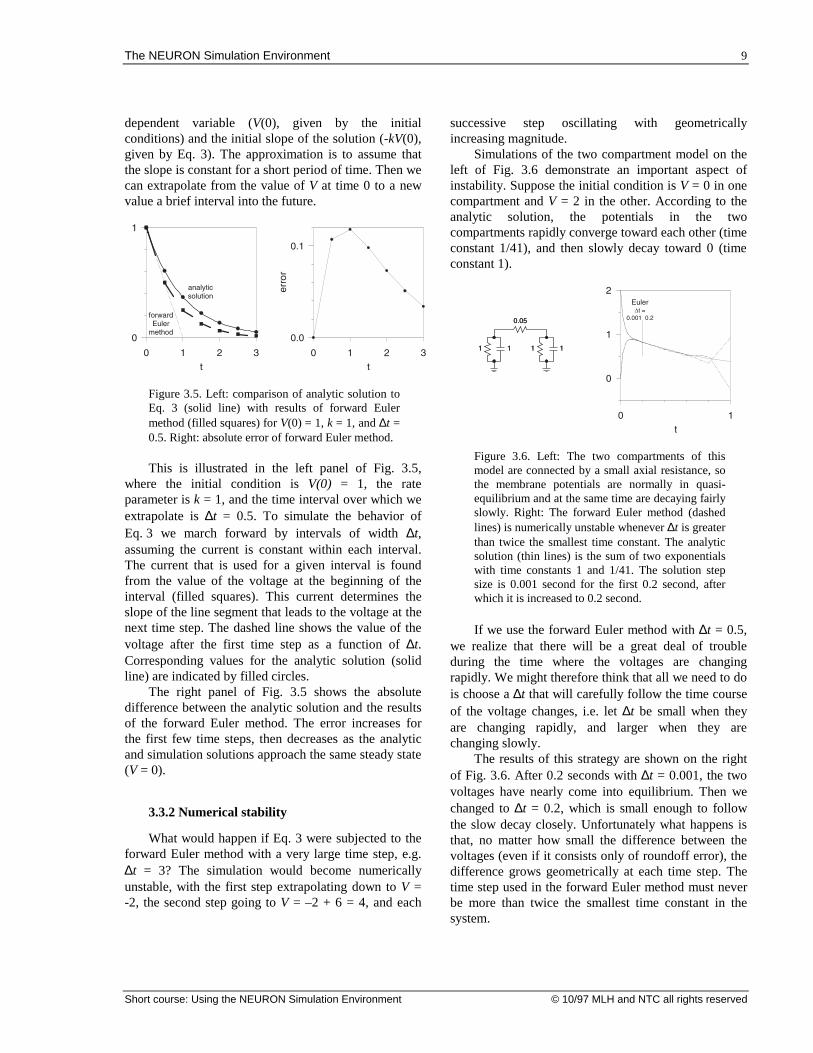
successive step oscillating with geometricallyincreasing magnitude.

Simulations of the two compartment model on theleft of Fig. 3.6 demonstrate an important aspect ofinstability. Suppose the initial condition is V = 0 in onecompartment and V = 2 in the other. According to theanalytic solution, the potentials in the twocompartments rapidly converge toward each other (timeconstant 1/41), and then slowly decay toward 0 (timeconstant 1).

Figure 3.6. Left: The two compartments of thismodel are connected by a small axial resistance, sothe membrane potentials are normally in quasi-equilibrium and at the same time are decaying fairlyslowly. Right: The forward Euler method (dashedlines) is numerically unstable whenever ∆t is greaterthan twice the smallest time constant. The analyticsolution (thin lines) is the sum of two exponentialswith time constants 1 and 1/41. The solution stepsize is 0.001 second for the first 0.2 second, afterwhich it is increased to 0.2 second.

If we use the forward Euler method with ∆t = 0.5,we realize that there will be a great deal of troubleduring the time where the voltages are changingrapidly. We might therefore think that all we need to dois choose a ∆t that will carefully follow the time courseof the voltage changes, i.e. let ∆t be small when theyare changing rapidly, and larger when they arechanging slowly.

The results of this strategy are shown on the rightof Fig. 3.6. After 0.2 seconds with ∆t = 0.001, the twovoltages have nearly come into equilibrium. Then wechanged to ∆t = 0.2, which is small enough to followthe slow decay closely. Unfortunately what happens isthat, no matter how small the difference between thevoltages (even if it consists only of roundoff error), thedifference grows geometrically at each time step. Thetime step used in the forward Euler method must neverbe more than twice the smallest time constant in thesystem.



Linear algebra clarifies the notion of “timeconstant” and its relationship to stability. For a linearsystem with N compartments, there are exactly Nspatial patterns of voltage over all compartments suchthat only the amplitude of the pattern changes withtime, while the shape of the pattern is preserved. Theamplitude of each of these patterns, or eigenvectors, is

given by et iλ , where λi is called the eigenvalue of theith eigenvector. Each eigenvalue is the reciprocal ofone of the time constants of the solutions to thedifferential equations that describe the system. The ithpattern decays exponentially to 0 if the real part of λi isnegative; if the real part is positive, the amplitudegrows catastrophically. If λi has an imaginarycomponent, the pattern oscillates with frequency ωi =Im(λi).

Our two compartment model has two such patterns.In one, the voltages in the two compartments areidentical. This pattern decays with the time course e –t.The other pattern, in which the voltages in the twocompartments are equal but have opposite sign, decayswith the much faster time course e –41t.

The key idea is that a problem involving N coupleddifferential equations can always be transformed into aset of N independent equations, each of which is solvedseparately as in the single compartment of Eq. 3. Whenthe equations that describe such a system are solvednumerically, the time step ∆t must be small enough thatthe solution of each equation is stable. This is thereason why stability criteria that involve ∆t depend onthe smallest time constant.

If the ratio between the slowest and fastest timeconstants is large, the system is said to be stiff.Stiffness is a serious problem because a simulation mayhave to run for a very long time in order to showchanges governed by the slow time constant, yet a small∆t has to be used to follow changes due to the fast timeconstant.

A driving force may alter the time constants thatdescribe a system, thereby changing its stabilityproperties. A current source (perfect current clamp)does not affect stability because it does not change thetime constants. Any other signal source imposes a loadon the compartment to which it is attached, changingthe time constants and their correspondingeigenvectors. The more closely it approximates avoltage source (perfect voltage clamp), the greater thiseffect will be.

3.3.3 The backward Euler method: inaccuratebut stable

The numerical stability problems of the forwardEuler method can be avoided if the equations areevaluated at time t + ∆t, i.e.

V t t V t tf V t t t t+ = + + +∆ ∆ ∆ ∆b g b g b gc h, (5)

Equation 5 can be derived from Taylor’s seriestruncated at the ∆t term but with t + ∆t in place of t.Therefore this approach is called the implicit orbackward Euler method.

For our one-compartment example, the backwardEuler method gives

V t tV t

k t+ =

+∆

∆b g b g

1(6)

Several iterations of Eq. 6 are shown in Fig. 3.7. Eachstep moves to a new point (ti+i, V(ti+1)) such that theslope there points back to the previous point (ti, V(ti)).If ∆t is very large, the solution converges exponentiallytoward the steady state instead of oscillating withgeometrically increasing amplitude.

Figure 3.7. Comparison of analytic solution to Eq. 3with results from backward Euler method (Eq. 6)for V(0) = 1, k = 1, and ∆t = 0.75. At the end ofeach step the slope at the new value points back tothe beginning of the step. The dashed line shows thevoltage after the first time step as a function of ∆t.

Applying the implicit method to the twocompartment model demonstrates its attractive stabilityproperties (Fig. 3.8). Notice that a large ∆t gives areasonable qualitative understanding of the behavior,even if it does not allow us to follow the initial rapidvoltage changes. Furthermore the step size can bechanged according to how quickly the states arechanging, yet the solution remains stable.



Figure 3.8. Two compartments as in Fig. 3.6simulated with backward Euler method. Left: ∆t =0.2 second, much larger than the fast time constant.Right: for the first 0.2 second, ∆t is small enough toaccurately follow the fast time constant. Thereafter,∆t is increased to 0.2 second, yet the simulationremains numerically stable.

The backward Euler method requires the solutionof a set of nonlinear simultaneous equations at eachstep. To compensate for this extra work, the step sizeneeds to be as large as possible while preserving goodquantitative accuracy. The first order implicit method ispractical for initial exploratory simulations becausereasonable values of ∆t produce fast simulations thatare almost always qualitatively correct, and tightlycoupled compartments do not generate large erroroscillations but instead come quickly into equilibriumbecause of its robust stability properties.

3.3.4 Error

The total or global error is a combination of errorsfrom two sources. The local error emerges from theextrapolation process within a time step. For thebackward Euler method this is easily analyzed withTaylor’s theorem truncated at the term proportional to∆t.

V t t V t tV t t

tV t

+ = + ′ +

− ′′

∆ ∆ ∆

∆

b g b g b g

b g2

2*

(7)

where t t t t≤ ≤ +* ∆

Both the forward and backward Euler methodsignore second and higher order terms, so the error ateach step is proportional to ∆t

2. Integrating over a fixedtime interval T requires T/∆t steps, so the error thataccumulates in this interval is on the order of

∆ ∆t T t2 ⋅ , i.e. the net error is proportional to ∆t.Therefore we can always decrease the local error asmuch as we like by reducing ∆t.

The second contribution to the total error comesfrom with the cumulative effect of past errors, whichhave moved the computed solution away from thetrajectory of the analytic solution. Thus, if ourcomputer solution has a nonzero total error at time t1,then even if we were to thereafter solve the equationsexactly using the state values at t1 as our initialcondition, the future solution will be inaccurate becausewe are on a different trajectory.

The total error of the simulation is therefore noteasy to analyze. In the example of Fig. 3.5, alltrajectories end up at the same steady state so totalerror tends to decrease, but not all systems behave inthis manner. Particularly treacherous are systems thatbehave chaotically so that, once the computed solutiondiverges even slightly from the proper trajectory, itsubsequently moves rapidly away from the original andthe time evolution becomes totally different.

The question is not so much how large the error ofa simulation is relative to the analytic solution, butwhether the simulation error leads us to trajectories thatare different from the set of trajectories defined by theerror in our parameters. There may be some benefit intreating the model equations as sacred runes whichmust be solved to an arbitrarily high precision, insofaras removal of any source of error has value.Nevertheless, judgment is required in order todetermine the meaning of a simulation run.

For example, consider the Hodgkin-Huxleymembrane action potentials elicited by two currentstimuli, one brief and strong and the other muchweaker. The left panel of Fig. 3.9 compares the resultsof computing these action potentials by the backwardEuler method using time steps of 25 and 5 µs. As notedabove, shortening the time step decreases thesimulation error. The effect is most noticeable forsimulations involving the weaker stimulus: while thevoltage hovers near threshold, a small error due to ourtime step grows into a large error in the time ofoccurrence of the spike.

However the behavior near threshold is highlysensitive to almost any parameter. This is demonstratedin the right of Fig. 3.9, where the sodium channeldensity is varied by only 1%. Clearly it is crucial toknow the sensitivity of our results to every parameter ofthe model, and the time step is just one more parameterwhich is added as a condition of being able to simulatea model on the computer.



Figure 3.9. Backward Euler method simulations ofHodgkin Huxley membrane action potentialselicited by a current stimulus of duration 0.3 ms andamplitude 0.8 mA/cm2 or 0.22 mA/cm2. Left:Sensitivity to integration time step. The solid anddashed traces were computed with ∆t = 25 and 5 µs,respectively. All action potentials were calculatedwith peak sodium conductance ( gNa ) 0.12siemens/cm2. Right: Sensitivity to gNa . All traces

were computed with ∆t = 5 µs. Peak sodiumconductance was 0.12 siemens/cm2 (solid lines) ±1% (dashed lines). The three simulations thatinvolved the large stimulus are indistinguishable inthis plot.

Using extremely small ∆t might seem to be the bestway to reduce error. However, computers represent realnumbers as floating point numbers with a fixed numberof digits, so if you keep adding 10–20 to 1 you mayalways get a value of 1, even after repeating the process1020 times. Operations that involve the difference ofsimilar numbers, as when differences are substituted forderivatives, are especially prone to such roundoff error.Consequently there is a limit to the accuracyimprovement that can be achieved by decreasing ∆t.

Generally speaking it would be nice to be able touse what might be called “physiological” values of ∆t,i.e. time steps that give a good representation of thestate trajectories without having a numerical accuracythat is many orders of magnitude better than theaccuracy of our physiological measurements.

3.3.5 Crank-Nicholson Method: stable andmore accurate

This motivates us to look into an integrationstrategy that combines the backward and forward Eulermethods. The central difference or Crank-Nicholsonmethod [Crank and Nicholson 1947], which isequivalent to advancing by one half step usingbackward Euler and then advancing by one half step

using forward Euler, has global error proportional tothe square of the step size. Fig. 3.10 illustrates the idea.The value at the end of each step is along a linedetermined by the estimated slope at the midpoint ofthe step.

Generally, for a given ∆t we can expect a largeaccuracy increase with the Crank-Nicholson method. Infact, the simulation using the 0.75 second time step inFig. 3.10 is much more accurate than the 0.5 secondtime step simulation with the forward Euler method(Fig. 3.5).

Figure 3.10. In the Crank-Nicholson method theslope at the midpoint of the step is used todetermine the new value. The analytic and Crank-Nicholson solutions are almost indistinguishable inthis figure. The dashed line shows the voltage afterthe first time step as a function of ∆t.

A most convenient feature of the central differencemethod is that the amount of computational work forthe extra accuracy beyond the backward Euler methodis trivial, since after computing V(t + ∆t/2) we just have

V t t V tt

V t+ = +FHG

IKJ −∆ ∆b g b g2

2(8)

so the extra accuracy does not cost extra computationsof the model functions.

One might well ask what effect the forward Eulerhalf step has on numerical stability. Fig. 3.11 shows thesolution for the two compartment model of Fig. 5computed using this central difference method, inwhich ∆t was much larger than the fast time constant.The sequence of a backward Euler half step followedby a forward Euler half step approximates anexponential decay by

V t t V t

k t

k t+ =

−

+∆

∆

∆b g b g1

2

12

(9)



As ∆t gets very large, the step multiplier approaches –1from above so the solution oscillates with decreasingamplitude.

Figure 3.11. The Crank-Nicholson method can havesignificant error oscillations when there is a largeamplitude component in the simulation that has atime constant much smaller than ∆t. However, theoscillation amplitude decreases at each step, so thesimulation is numerically stable.

Technically speaking the Crank-Nicholson methodis stable because the error oscillations do decay withtime. However, this example shows that it can produceartifactual large amplitude oscillations if the time stepis too large. This can affect simulations of models thatinvolve voltage clamps or in which adjacent segmentsare coupled by very small resistances.

3.3.6 The integration methods used inNEURON

The preceding discussion shows why NEURONoffers the user a choice of two stable implicitintegration methods: backward Euler, and a variant ofCrank-Nicholson. Because of its robust numericalstability properties, backward Euler produces goodqualitative results even with large time steps, and itworks even if some or all of the equations are strictlyalgebraic relations among states. It can be used withextremely large time steps to find the steady-statesolution for a linear (“passive”) system. BackwardEuler is therefore the default integrator used byNEURON.

When the global parameter secondorder is setto 2, a variant of the Crank-Nicholson method is used,which has numerical error proportional to ∆t2 and istherefore more accurate for small time steps.

In implicit integration methods, all current balanceequations must be solved simultaneously. Thebackward Euler algorithm does not resort to iteration to

deal with nonlinearities, since its numerical error isproportional to ∆t anyway. The special feature of theCrank-Nicholson variant is its use of a staggered timestep algorithm to avoid iteration of nonlinear equations(see 3.3.7 Efficiency below). This converts the currentbalance part of the problem to one that requires onlythe solution of simultaneous linear equations.

Although the Crank-Nicholson method is formallystable, it is sometimes plagued by spurious largeamplitude oscillations (Fig. 3.11). This occurs when ∆tis too large, as may occur in models that involve fastvoltage clamps or that have compartments which arecoupled by very small resistances. However, Crank-Nicholson is safe in most situations, and it can be muchmore efficient than backward Euler for a givenaccuracy.

These two methods are almost identical in terms ofcomputational cost per time step (see 3.3.7 Efficiencybelow). Since the current balance equations have thestructure of a tree (there are no current loops), directgaussian elimination is optimal for their solution (Hines1984). This takes exactly the same number of computeroperations as would be required for an unbranchedcable with the same number of compartments.

For any particular problem, the best way todetermine which is the method of choice is to compareboth methods with several values of ∆t to see whichallows the largest ∆t consistent with the desiredaccuracy. In performing such trials, one must rememberthat the stability properties of a simulation depend onthe entire system that is being modeled. Because ofinteractions between “biological” components and any“nonbiological” elements, such as stimulators orvoltage-clamps, the time constants of the entire systemmay be different from those of the biologicalcomponents alone. A current source (perfect currentclamp) does not affect stability because it does notchange the time constants. Any other signal sourceimposes a load on the compartment to which it isattached, changing the time constants and potentiallyrequiring use of a smaller time step to avoid numericaloscillations in the Crank-Nicholson method. The moreclosely a signal source approximates a voltage source(perfect voltage clamp), the greater this effect will be.

3.3.7 Efficiency

Nonlinear equations generally need to be solvediteratively to maintain second order correctness.However, voltage dependent membrane properties,which are typically formulated in analogy to Hodgkin-



Huxley (HH) type channels, allow the cable equation tobe cast in a linear form, still second order correct, thatcan be solved without iterations. A direct solution ofthe voltage equations at each time step t → t + ∆t usingthe linearized membrane current I(V,t) = G · (V – E) issufficient as long as the slope conductance G and theeffective reversal potential E are known to second orderat time t + 0.5 ∆t. HH type channels are easy to solve att + 0.5 ∆t since the conductance is a function of statevariables which can be computed using a separate timestep that is offset by 0.5 ∆t with respect to the voltageequation time step. That is, to integrate a state from t- 0.5 ∆t to t + 0.5 ∆t we only require a second ordercorrect value for the voltage dependent rates at themidpoint time t.

Figure 3.12. The equations shown here arecomputed using the Crank-Nicholson method. Top:x(t + ∆t) and y(t + ∆t) are determined using theirvalues at time t. Bottom: staggered time steps yielddecoupled linear equations. y(t + ∆t/2) isdetermined using x(t), after which x(t + ∆t) isdetermined using y(t + ∆t/2).

Figure 3.12 contrasts this approach with thecommon technique of replacing nonlinear coefficientsby their values at the beginning of a time step. For HHequations in a single compartment, the staggered timegrid approach converts four simultaneous nonlinearequations at each time step to four independent linearequations that have the same order of accuracy at each

time step. Since the voltage dependent rates use thevoltage at the midpoint of the integration step,integration of channel states can be done analytically injust a single addition and multiplication operation andtwo table lookup operations. While this efficientscheme achieves second order accuracy, the tradeoff isthat the tables depend on the value of the time step andmust be recomputed whenever the time step changes.

Neuronal architecture can also be exploited toincrease computational efficiency. Since neuronsgenerally have a branched tree structure with no loops,the number of arithmetic operations required to solvethe cable equation by Gaussian elimination is exactlythe same as for an unbranched cable with the samenumber of compartments. That is, we need only O(N)arithmetic operations for the equations that describe Ncompartments connected in the form of a tree, eventhough standard Gaussian elimination generally takesO(N3) operations to solve N equations in N unknowns.

The tremendous efficiency increase results fromthe fact that, in a tree, one can always find a leafcompartment i that is connected to only one othercompartment j, so that

a V a V bii i ij j i+ = (10a)

a V a V

b

ji i jj j

j

+ +

=

terms from other compartments

(10b)

In other words, the equation for compartment i(Eq. 10a) involves only the voltages in compartments iand j, and the voltage in compartment i appears only inthe equations for compartments i and j (Eq. 10a and b).Using Eq. 10a to eliminate the Vi term from Eq. 10b,which requires O(1) (instead of N) operations, givesEq. 11 and leaves N–1 equations in N–1 unknowns.

′ +

= ′

a V

b

jj j

j

terms from other compartments

(11)

where ′ = −a a a a ajj jj ij ji iid iand ′ = −b b b a aj j i ji iid i

This strategy can be applied until there is only oneequation in one unknown.

Assume that we know the solution to these N–1equations, and in particular that we know Vj. Then wecan find Vi from Eq. 10a with O(1) step. Therefore the



effort to solve these N equations is O(1) plus the effortneeded to solve N–1 equations. The number ofoperations required is independent of the branchingstructure, so a tree of N compartments uses exactly thesame number of arithmetic operations as a one-dimensional cable of N compartments.

Efficient Gaussian elimination requires an orderingthat can be found by a simple algorithm: choose theequation with the current minimum number of terms asthe equation to use in the elimination step. Thisminimum degree ordering algorithm is commonlyemployed in standard sparse matrix solver packages.For example, NEURON’s “Matrix” class uses thematrix library written by Stewart and Leyk (1994). Thisand many other sparse matrix packages are freelyavailable at http://www.netlib.org.

4. THE NEURON SIMULATION

ENVIRONMENT

No matter how powerful and robust itscomputational engine may be, the real utility of anysoftware tool depends largely on its ease of use.Therefore a great deal of effort has been invested in thedesign of the simulation environment provided byNEURON. In this section we first briefly considergeneral aspects of the high-level language used forwriting NEURON programs. Then we turn to anexample of a model of a nerve cell to introduce specificaspects of the user environment, after which we coverthese features more thoroughly.

4.1 The hoc interpreter

NEURON incorporates a programming languagebased on hoc, a floating point calculator with C-likesyntax described by Kernighan and Pike (1984). Thisinterpreter has been extended by the addition of object-oriented syntax (not including polymorphism orinheritance) that can be used to implement abstract datatypes and data encapsulation. Other extensions includefunctions that are specific to the domain of neuralsimulations, and functions that implement a graphicaluser interface (see below).

With hoc one can quickly write short programsthat meet most problem-specific needs. The interpreteris used to execute simulations, customize the userinterface, optimize parameters, analyze experimentaldata, calculate new variables such as impulsepropagation velocity, etc..

NEURON simulations are not subject to theperformance penalty often associated with interpreted(as opposed to compiled) languages becausecomputationally intensive tasks are carried out byhighly efficient precompiled code. Some of these tasksare related to integration of the cable equation andothers are involved in the emulation of biologicalmechanisms that generate and regulate chemical andelectrical signals.

NEURON provides a built-in implementation ofthe microemacs text editor. Since the choice of aprogramming editor is highly personal, NEURON willalso accept hoc code in the form of straight ASCIIfiles created with any other editor.

4.2 A specific example

In the following example we show how NEURONmight be used to model the cell in the top of Fig. 4.1.Comments in the hoc code are preceded by doubleslashes (//), and code blocks are enclosed in curlybrackets (). Because the model is described in apiecewise fashion and many of the code specimensgiven below are meant to illustrate other features ofNEURON, for the sake of clarity a fully commentedand complete listing of the hoc code for this model iscontained in Appendix 1.

Figure 4.1. Top: cartoon of a neuron with a soma,three dendrites, and an unmyelinated axon (not toscale). The soma diameter is 50 µm. Each dendriteis 200 µm long and tapers uniformly along itslength from 10 µm diameter at the soma to 3 µm atits distal end. The unmyelinated cylindrical axon is1000 µm long and has a diameter of 1 µm. Anelectrode (not shown) is inserted into the soma forintracellular injection of a stimulating current.Bottom: topology of a NEURON model thatrepresents this cell.



4.2.1 First step: establish model topology

One very important feature of NEURON is that itallows the user to think about models in terms that arefamiliar to the neurophysiologist, keeping numericalissues (e.g. number of spatial segments) entirelyseparate from the specification of morphology andbiophysical properties. As noted in a previous section(3.2 Spatial discretization . . . ), this separation isachieved through the use of one-dimensional cable“sections” as the basic building block from whichmodel cells are constructed. These sections can beconnected together to form any kind of branched cableand endowed with properties which may vary withposition along their length.

The idealized neuron in Fig. 4.1 has severalanatomical features whose existence and spatialrelationships we want the model to include: a cell body(soma), three dendrites, and an unmyelinated axon. Thefollowing hoc code sets up the basic topology of themodel:

create soma, axon, dendrite[3]connect axon(0), soma(0)for i=0,2 connect dendrite[i](0), soma(1)

The program starts by creating named sections thatcorrespond to the important anatomical features of thecell. These sections are attached to each other usingconnect statements. As noted previously, eachsection has a normalized position parameter x whichranges from 0 at one end to 1 at the other. Because theaxon and dendrites arise from opposite sides of the cellbody, they are connected to the 0 and 1 ends of thesoma section (see bottom of Fig. 4.1). A child sectioncan be attached to any location on the parent, butattachment at locations other than 0 or 1 is generallyemployed only in special cases such as spines ondendrites.

4.2.2 Second step: assign anatomical andbiophysical properties

Next we set the anatomical and biophysicalproperties of each section. Each section has its ownsegmentation, length, and diameter parameters, so it isnecessary to indicate which section is being referenced.There are several ways to declare which is the currentlyaccessed section, but here the most convenient is toprecede blocks of statements with the appropriatesection name.

soma nseg = 1 L = 50 // [µm] length diam = 50 // [µm] diameter insert hh // HH currents gnabar_hh = 0.5*0.120 // [S/cm 2]axon nseg = 20 L = 1000 diam = 1 insert hhfor i=0,2 dendrite[i] nseg = 5 L = 200 diam(0:1) = 10:3 // tapers insert pas // passive current e_pas = -65 // [mv] eq potential g_pas = 0.001 // [S/cm 2]

The fineness of the spatial grid is determined bythe compartmentalization parameter nseg (see3.2 Spatial discretization . . . ). Here the soma islumped into a single compartment (nseg = 1), whilethe axon and each of the dendrites are broken intoseveral subcompartments (nseg = 20 and 5,respectively).

In this example, we specify the geometry of eachsection by assigning values directly to section lengthand diameter. This creates a “stylized model.”Alternatively, one can use the “3-D method,” in whichNEURON computes section length and diameter from alist of (x, y, z, diam) measurements (see 4.5 Specifyinggeometry: stylized vs. 3-D).

Since the axon is a cylinder, the correspondingsection has a fixed diameter along its entire length. Thespherical soma is represented by a cylinder with thesame surface area as the sphere. The dimensions andelectrical properties of the soma are such that itsmembrane will be nearly isopotential, so the cylinderapproximation is not a significant source of error. Ifchemical signals such as intracellular ionconcentrations were important in this model, it wouldbe necessary to approximate not only the surface areabut also the volume of the soma.

Unlike the axon, the dendrites becomeprogressively narrower with distance from the soma.Furthermore, unlike the soma, they are too long to belumped into a single compartment with constantdiameter. The taper of the dendrites is accommodatedby assigning a sequence of decreasing diameters totheir segments. This is done through the use of “rangevariables,” which are discussed below (4.4 Rangevariables).



In this model the soma and axon contain Hodgkin-Huxley (HH) sodium, potassium, and leak channels(Hodgkin and Huxley 1952), while the dendrites haveconstant, linear (“passive”) ionic conductances. Theinsert statement assigns the biophysical mechanismsthat govern electrical signals in each section. Particularvalues are set for the density of sodium channels on thesoma (gnabar_hh) and for the ionic conductance andequilibrium potential of the passive current in thedendrites (g_pas and e_pas). More informationabout membrane mechanisms is presented in a latersection (4.6 Density mechanisms and pointprocesses).

4.2.3 Third step: attach stimulating electrodes

This code emulates the use of an electrode to injecta stimulating current into the soma by placing a currentpulse stimulus in the middle of the soma section. Thestimulus starts at t = 1 ms, lasts for 0.1 ms, and has anamplitude of 60 nA.

objref stim// put stim in middle of somasoma stim = new Iclamp(0.5)stim.del = 1 // [ms] delaystim.dur = 0.1 // [ms] durationstim.amp = 60 // [nA] amplitude

The stimulating electrode is an example of a pointprocess. Point processes are discussed in more detailbelow (4.6 Density mechanisms and point processes).

4.2.4 Fourth step: control simulation timecourse

At this point all model parameters have beenspecified. All that remains is to define the simulationparameters, which govern the time course of thesimulation, and write some code that executes thesimulation.

This is generally done in two procedures. The firstprocedure initializes the membrane potential and thestates of the inserted mechanisms (channel states, ionicconcentrations, extracellular potential next to themembrane). The second procedure repeatedly calls thebuilt-in single step integration function fadvance()and saves, plots, or computes functions of the desiredoutput variables at each step. In this procedure it ispossible to change the values of model parametersduring a run.

The built-in function finitialize() initializestime t to 0, membrane potential v to -65 mvthroughout the model, and the HH state variables m, nand h to their steady state values at v = –65 mv.Initialization can also be performed with a user-writtenroutine if there are special requirements thatfinitialize() cannot accommodate, such asnonuniform membrane potential.

dt = 0.05 // [ms] time steptstop = 5 // [ms]

// initialize membrane potential,// state variables, and timefinitialize(-65)

proc integrate() // show somatic Vm at t=0print t, soma.v(0.5)while (t < tstop)

// advance solution by dtfadvance()// function calls to save// or plot results// would go here// show time and soma Vmprint t, soma.v(0.5)// statements that change// model parameters// would go here

Both the integration time step dt and the solutiontime t are global variables. For this example dt =50 µs. The while() statement repeatedly callsfadvance(), which integrates the model equationsover the interval dt and increments t by dt on eachcall. For this example, the time and somatic membranepotential are displayed at each step. This loop exitswhen t ≥ tstop.

The entire listing of the hoc code for the model isprinted in Appendix 1. When this program is firstprocessed by the NEURON interpreter, the model is setup and initiated but the integrate() procedure isnot executed. When the user enters an integrate()statement in the NEURON interpreter window, thesimulation advances for 5 ms using 50 µs time steps.

4.3 Section variables

Three parameters apply to the section as a whole:cytoplasmic resistivity Ra (Ω cm), the section length L,and the compartmentalization parameter nseg. Thefirst two are “ordinary” in the sense that they do not



affect the structure of the equations that describe themodel. Note that the hoc code specifies values for Lbut not for Ra. This is because each section in a modelis likely to have a different length, whereas thecytoplasm (and therefore Ra) is usually assumed to beuniform throughout the cell. The default value of Ra is35.4 Ω cm, which is appropriate for invertebrateneurons. Like L it can be assigned a new value in anyor all sections (e.g. ~200 Ω cm for mammalianneurons).

The user can change the compartmentalizationparameter nseg without having to modify any of thestatements that set anatomical or biophysical properties.However, if parameters vary with position in a section,care must be taken to ensure that the modelincorporates the spatial detail inherent in the parameterdescription.

4.4 Range variables

Like dendritic diameter in our example, mostcellular properties are functions of the positionparameter x. NEURON has special provisions fordealing with these properties, which are called “rangevariables.” Other examples of range variables includethe membrane potential v, and ionic conductanceparameters such as the maximum HH sodiumconductance gnabar_hh (siemens / cm2).

Range variables enable the user to separateproperty specification from segment number. A rangevariable is assigned a value in one of two ways. Thesimplest and most common is as a constant. Forexample, the statement axon.diam = 10 assertsthat the diameter of the axon is uniform over its entirelength.

Properties that change along the length of a sectionare specified with the syntaxrangevar(xmin:xmax) = e1:e2. The fouritalicized symbols are expressions with e1 and e2being the values of the property at xmin and xmax,respectively. The position expressions must meet theconstraint 0 ≤ xmin ≤ xmax ≤ 1. Linear interpolationis used to assign the values of the property at thesegment centers that lie in the position range [xmin,xmax]. In this manner a continuously varying propertycan be approximated by a piecewise linear function. Ifthe range variable is diameter, neither e1 nor e2should be 0, or the corresponding axial resistance willbe infinite.

In our model neuron, the simple dendritic taper isspecified by diam(0:1) = 10:3 and nseg = 5.

This results in five segments that have centers at x =0.1, 0.3, 0.5, 0.7 and 0.9 and diameters of 9.3, 7.9, 6.5,5.1 and 3.7, respectively.

To underscore the relationship between parameterranges, segment centers, and the values that areassigned to range variables, it may be helpful toconsider a pair of examples. The second column ofTable 4.1 shows the values of x at which segmentcenters would be located for nseg = 1, 2, 3 and 5. Thethird column shows the corresponding diameters ofthese segments for a dendrite with a diameter of 10 µmover the first 60% of its length and 14 µm over theremaining 40% of its length. The diameter that isassigned to each segment depends entirely on whetherthe segment center lies in the x interval thatcorresponds to 10 µm or 14 µm.

nseg

segmentcentersx see Note 1 see Note 2

1 0.5 10 13

20.250.75

1014

10.514

30.1667

0.50.8333

101014

101314

5

0.10.30.50.70.9

1010101414

1011131414

Note 1 diam(0:0.6)=10:10diam(0.6:1)=14:14

Note 2 diam(0:0.2)=10:10diam(0.6:1)=14:14diam(0.2:0.6)=10:14

Table 4.1. Diameter as a range variable: effects ofnseg on segment diameters

The fourth column illustrates interpolation ofsegment diameters. Here the dendrite starts with adiameter of 10 µm over the first 20% of its length, hasa linear flare from 10 to 14 µm over the next 40%, andends with a diameter of 14 µm over the last 40% of itslength. The segments that have centers in the interval[0.2, 0.6] are assigned diameters that are interpolated.

The value of a range variable at the center of asegment can appear in any expression using the syntaxrangevar(x) in which 0 ≤ x ≤ 1. The value returnedis the value at the center of the segment containing x,NOT the linear interpolation of the values stored at the



centers of adjacent segments. If the parentheses areomitted, the position defaults to a value of 0.5 (middleof the section).

A special form of the for statement is available:for (var) stmt. For each value of the normalizedposition parameter x that defines the center of eachsegment in the selected section (along with positions 0and 1), this statement assigns var that value andexecutes the stmt. This hoc code would print themembrane potential as a function of physical position(in µm) along the axon:

axon for (x) print x*L, v(x)

4.5 Specifying geometry: stylized vs.3-D

As noted above (4.2.2 Second step . . . ), there aretwo ways to specify section geometry. Our exampleuses the stylized method, which simply assigns valuesto section length and diameter. This is most appropriatewhen cable length and diameter are authoritative and 3-D shape is irrelevant.

It is best to use the 3-D method if the model isbased on anatomical reconstruction data (quantitativemorphometry), or if 3-D visualization is paramount.This approach keeps the anatomical data in a list of (x,y, z, diam) “points.” The first point is associated withthe end of the section that is connected to the parent(this is not necessarily the 0 end!) and the last point isassociated with the opposite end. There must be at leasttwo points per section, and they should be ordered interms of monotonically increasing arc length. This pt3dlist, which is the authoritative definition of the shape ofthe section, automatically determines the length anddiameter of the section.

When the pt3d list is non-empty, the shape modelused for a section is a sequence of frusta. The pt3dpoints define the locations and diameters of the ends ofthese frusta. The effective area, diameter, andresistance of each segment are computed from thissequence of points by trapezoidal integration along thesegment length. This takes into account the extra areaintroduced by diameter changes; even degenerate conesof 0 length can be specified (i.e. two points with samecoordinates but different diameters), which add area butnot length to the section. No attempt is made to dealwith the effects of centroid curvature on surface area.The number of 3-D points used to describe a shape hasnothing to do with nseg and does not affect simulationspeed.

When diameter varies along the length of a section,the stylized and 3-D approaches to defining sectionstructure can lead to very different modelrepresentations, even when the specifications mightseem to be identical. Imagine a cell whose diametervaries with position x as shown in Fig. 4.2

Figure 4.2. A hypothetical cell whose structure is tobe approximated using the stylized and 3-Dapproaches.

This program contrasts the results of using thestylized and 3-D approaches to emulate the structure ofthis cell. It creates sections stylized_model andthree_d_model, whose geometries are specifiedusing the stylized and 3-D methods, respectively. Foreach segment of these two sections, it prints out the xlocation of the segment center, the segment diameterand surface area, and the axial resistance ri (inmegohms) between the segment center and the centerof the parent segment (i.e. the segment centered at thenext smaller x; see the Ri in Fig. 3.3).

/* diampt3d.hoc */

create stylized_model, three_d_model

// set nseg and L for both modelsforall nseg = 5 L = 1

stylized_model diam(0:0.3) = 0:3 diam(0.3:0.7) = 3:3 diam(0.7:1) = 3:0

three_d_model pt3dadd(0,0,0,0) pt3dadd(0.3,0,0,3) pt3dadd(0.7,0,0,3) pt3dadd(1,0,0,0)

forall print secname() for (x) print x,diam(x),area(x),ri(x)

The output of this program is presented inTable 4.2. The stylized approach creates a section



composed of a series of cylindrical segments whosediameters are interpolated from the range variablespecification of diameter (left panel of Fig. 4.3). Thesurface areas and axial resistances associated with thesecylinders are based entirely on their cylindricaldimensions.

Figure 4.3. Left: The stylized representation of thehypothetical cell shown in Fig. 4.2. Right: In the3-D approach, the diameter, surface area, and axialresistance of each segment are based on theintegrals of these quantities over the correspondinginterval in the original anatomy.

The 3-D approach, however, produces a model thatis quite different. The reported diameter of eachsegment, diam(x), is the average diameter over thecorresponding length of the original anatomy, and thesegment area, area(x), is the integral of the surfacearea. Therefore area(x) is not necessarily equal toπ diam(x) L / nseg. The axial resistances arecomputed by integrating the resistance of the cytoplasmalong the path between the centers of adjacentsegments. Both ri(0) and ri(1) are effectivelyinfinite because the diameter of the volume elementsalong the integration path tapers to 0 at both ends of the3-D data set.

Close examination of Table 4.2 reveals two itemsthat require additional comment. The first item is thatri(0) = 1030 for both models. This is because,regardless of whether the stylized or the 3-D approachis used, the left hand side of the section is a “sealedend” or open circuit.

The second noteworthy item, which at first seemsunexpected, is that even though the diameter isspecified to be 0 at x = 0 and 1, the model generated by

the 3-D approach reports nonzero values for diam(0)and diam(1). This reflects the fact that, except formembrane potential v, accessing the value of a rangevariable at x = 0 or 1 returns the value at the center ofthe first and last segment, respectively (i.e. at x =0.5/nseg and 1 – 0.5/nseg). The technical reason forthis behavior is that diameter is part of a morphologymechanism, and mechanisms exist only in the interiorof a section. As noted in 4.4 Range variables,range_variable(x) returns the value of the rangevariable at the center of the segment that contains x.The only range variable that exists at the 0 and 1locations is v; other range variables are undefined atthese points (area() and ri() are functions, notrange variables). Point processes, which are discussednext, are not accessed as functions of position and canbe placed anywhere in the interval 0 ≤ x ≤ 1.

4.6 Density mechanisms and pointprocesses

The insert statement assigns biophysicalmechanisms, which govern electrical and (if present)chemical signals, to a section. Many sources ofelectrical and chemical signals are distributed over themembrane of the cell. These density mechanisms aredescribed in terms of current per unit area andconductance per unit area; examples include voltage-gated ion channels such as the HH currents.

However, density mechanisms are not the mostappropriate representation of all signal sources.Synapses and electrodes are best described in terms oflocalized absolute current in nanoamperes andconductance in microsiemens. These are called pointprocesses.

An object syntax is used to manage the creation,insertion, attributes, and destruction of point processes.For example, a current clamp (electrode for injecting acurrent) is created by declaring an object variable and

Stylized model 3-D modelx diam(x) area(x) ri(x) diam(x) area(x) ri(x)

0 1 0 1e+30 1 0 1e+300.1 1 0.628318 0.0450727 1 3.20381 4.50727e+140.3 3 1.88495 0.0500808 2.75 4.94723 0.03004850.5 3 1.88495 0.0100162 3 1.88495 0.01001620.7 3 1.88495 0.0100162 2.75 4.94723 0.01001620.9 1 0.628318 0.0500808 1 3.20381 0.03004851.0 1 0 0.0450727 1 0 4.50727e+14

Table 4.2. Diameter as a range variable:differences between models created by stylizedand 3-D methods for specifying section geometry.



assigning it a new instance of the IClamp object class(see 4.2.3 Third step: attach stimulating electrodes).When a point process is no longer referenced by anyobject variable, the point process is removed from thesection and destroyed. In our example, redeclaringstim with the statement objref stim woulddestroy the pulse stimulus, since no other objectvariable is referencing it.

The x position specified for a point process canhave any value in the range [0,1]. If x is specified to beat 0 or 1, it will be located at the corresponding end ofthe section. For specified locations 0 < x < 1, the actualposition used by NEURON will be the center ofwhichever segment contains x. For example, in asection with nseg = 5 the segment centers (internalnodes) are located at x = 0.1, 0.3, 0.5, 0.7 and 0.9.Point processes whose specified locations are 0.04 and0.41 would be assigned by NEURON to the nodes at0.1 and 0.5, respectively. The error introduced by this“shift” can be avoided by explicitly placing pointprocesses at internal nodes, and restricting changes ofnseg to odd multiples. However, this may not bepossible in models that are based closely on realanatomy, because actual synaptic locations are unlikelyto be situated precisely at the centers of segments. Tocompletely avoid nseg-dependent shifts of the xlocations of point processes, one can choose sectionswith lengths such that the point processes are located atthe 0 or 1 ends of sections.

The location of a point process can be changedwith no effect on its other attributes. In our example thestatement dendrite[2] stim.loc(1) wouldmove the current stimulus to the distal end of the thirddendrite.

If a section’s nseg is changed, that section’s pointprocesses are relocated to the centers of the newsegments that contain the centers of the old segments towhich the point processes had been assigned. When asegment is destroyed, as by re-creating the section, allof its point processes lose their attributes, including xlocation and which section they belong to.

Many user-defined density mechanisms and pointprocesses can be simultaneously present in eachcompartment of a neuron. One important differencebetween density mechanisms and point processes is thatany number of the same kind of point process can existat the same location.

User-defined density mechanisms and pointprocesses can be linked into NEURON using the modeldescription language NMODL. This lets the user focuson specifying the equations for a channel or ionicprocess without regard to its interactions with other

mechanisms. The NMODL translator then constructsthe appropriate C program which is compiled andbecomes available for use in NEURON. This programproperly and efficiently computes the total current ofeach ionic species used, as well as the effect of thatcurrent on ionic concentration, reversal potential, andmembrane potential. An extensive discussion ofNMODL is beyond the scope of this article, but itsmajor advantages can be listed succinctly.1. Interface details to NEURON are handled

automatically — and there are a great many suchdetails.• NEURON needs to know that model states are

range variables and which model parameterscan be assigned values and evaluated from theinterpreter.

• Point Processes need to be accessible via theinterpreter object syntax and densitymechanisms need to be added to a sectionwhen the “insert” statement is executed.

• If two or more channels use the same ion atthe same place, the individual currentcontributions need to be added together tocalculate a total ionic current.

2. Consistency of units is ensured.3. Mechanisms described by kinetic schemes are

written with a syntax in which the reactions areclearly apparent. The translator providestremendous leverage by generating a large block ofC code that calculates the analytic Jacobian and thestate fluxes.

4. There is often a great increase in clarity sincestatements are at the model level instead of the Cprogramming level and are independent of thenumerical method. For example, sets of differentialand nonlinear simultaneous equations are writtenusing an expression syntax such as

x’ = f(x, y, t)~ g(x, y) = h(x, y)

where the prime refers to the derivative withrespect to time (multiple primes such as x’’ referto higher derivatives) and the tilde introduces analgebraic equation. The algebraic portion of suchsystems of equations is solved by Newton’smethod, and a variety of methods are available forsolving the differential equations, such as Runge-Kutta or backward Euler.

5. Function tables can be generated automatically forefficient computation of complicated expressions.



6. Default initialization behavior of a channel can bespecified.

4.7 Graphical interface

The user is not limited to operating within thetraditional “code-based command-mode environment.”Among its many extensions to hoc, NEURON includesfunctions for implementing a fully graphical, windowedinterface. Through this interface, and without having towrite any code at all, the user can effortlessly createand arrange displays of menus, parameter value editors,graphs of parameters and state variables, and views ofthe model neuron. Anatomical views, called “spaceplots,” can be explored, revealing what mechanismsand point processes are present and where they arelocated.

The purpose of NEURON’s graphical interface isto promote a match between what the user thinks isinside the computer, and what is actually there. Thesevisualization enhancements are a major aid tomaintaining conceptual control over the simulationbecause they provide immediate answers to questionsabout what is being represented in the computer.

The interface has no provision for constructingneuronal topology, a conscious design choice based onthe strong likelihood that a graphical toolbox forbuilding neuronal topologies would find little use.Small models with simple topology are so easilycreated in hoc that a graphical topology editor isunnecessary. More complex models are toocumbersome to deal with using a graphical editor. It isbest to express the topological specifications ofcomplex stereotyped models through algorithms,written in hoc, that generate the topologyautomatically. Biologically realistic models ofteninvolve hundreds or thousands of sections, whosedimensions and interconnections are contained in largedata tables generated by hours of painstakingquantitative morphometry. These tables are commonlyread by hoc procedures that in turn create and connectthe required sections without operator intervention.

The basic features of the graphical interface andhow to use it to monitor and control simulations arediscussed elsewhere (Moore and Hines 1996).However, several sophisticated analyis and simulationtools that have special utility for nerve simulation areworthy of mention.• The “Function Fitter” optimizes a parameterized

mathematical expression to minimize the least

squared difference between the expression anddata.

• The “Run Fitter” allows one to optimize severalparameters of a complete neuron model toexperimental data. This is most useful in thecontext of voltage clamp data which iscontaminated by incomplete space clamp ormodels that cannot be expressed in closed form,such as kinetic schemes for channel conductance.

• The “Electrotonic Workbench” plots small signalinput and transfer impedance and voltageattenuation as functions of space and frequency(Carnevale et al. 1996). These plots include theneuromorphic (Carnevale et al. 1995) and L vs. x(O'Boyle et al. 1996) renderings of the electrotonictransformation (Brown et al. 1992; Tsai et al.1994b; Zador et al. 1995). By revealing theeffectiveness of signal transfer, the Workbenchquickly provides insight into the “functionalshape” of a neuron.

All interaction with these and other tools takes place inthe graphical interface and no interpreter programmingis needed to use them. However, they are constructedentirely within the interpreter and can be modifiedwhen special needs require.

4.8 Object-oriented syntax

4.8.1 Neurons

It is often convenient to deal with groups ofsections that are related. Therefore NEURON providesa data class called a SectionList that can be used toidentify subsets of sections. Section lists fit nicely withthe “regular expression” method of selecting sections,used in earlier implementations of NEURON, in that1. the section list is easily constructed by using

regular expressions to add and delete sections2. after the list is constructed it is available for reuse3. it is much more efficient to loop over the sections

in a section list than to pick out the sectionsaccepted by a combination of regular expressions

This code

objref alldendalldend = new SectionList()forsec "dend" alldend.append()forsec alldend print secname()

forms a list of all the sections whose names contain thestring “dend” and then iterates over the list, printing thename of each section in it. For the example program



presented in this report, this would generate thefollowing output in the NEURON interpreter window

dendrite[0]dendrite[1]dendrite[2]

although in this very simple example it would clearlyhave been easy enough to loop over the array ofdendrites directly, e.g.

for i = 0,2 dendrite[i] print secname()

4.8.2 Networks

To help the user manage very large simulations,the interpreter syntax has been extended to facilitate theconstruction of hierarchical objects. This is illustratedby the following code fragment, which specifies apattern for a simple stylized neuron consisting of threedendrites connected to one end of a soma and an axonconnected to the other end.

begintemplate Cellx public soma, dendrite, axon create soma, dendrite[3], axon proc init() for i=0,2 connect dendrite[i](0), soma(0) connect axon(0), soma(1) axon insert hh endtemplate Cellx

Whenever a new instance of this pattern is created, theinit() procedure automatically connects the soma,dendrite, and axon sections together. A completepattern would also specify default membrane propertiesas well as the number of segments for each section.

Names that can be referenced outside the patternare listed in the public statement. In this case, sinceinit is not in the list, the user could not re-initializeby calling the init() procedure. Public names arereferenced through a dot notation.

The particular benefit of using templates (“classes”in standard object oriented terminology) is the fact thatthey can be employed to create any number of instancesof a pattern. For example,

objref cell[10][10]for i=0,9

for j=0,9 cell[i][j]=new Cellx()

creates an array of 100 objects of type Cellx that canbe referenced individually via the object variablecell. In this example,

cell[4][5].axon.gnabar_hh(0.5)

is the value of the maximum HH sodium conductancein the middle of the axon of cell[4][5].

As this example implies, templates offer a naturalsyntax for the creation of networks. However it isentirely up to the user to logically organize thetemplates in such a way that they appropriately reflectthe structure of the problem. Generally, any givenstructural organization can be viewed as a hierarchy ofcontainer classes, such as cells, microcircuits, layers, ornetworks. The important issue is how much effort isrequired for the concrete network representation tosupport a range of logical views of the same abstractnetwork. A logical view that organizes the cellsdifferently may not be easy to compute if the network isbuilt as an elaborate hierarchy. This kind of pressuretends to encourage relatively flat organizations thatmake it easier to implement functions that search forspecific information. The bottom line is that networksimulation design remains an ad hoc process thatrequires careful programming judgement.

One very important class of logical views that arenot generally organizable as a hierarchy are those ofsynaptic organization. In connecting cells withsynapses, one is often driven to deal with generalgraphs, which is to say, no structure at all.

In addition to the notions of classes and objects (asynapse is an object with a pre- and a postsynapticlogical connection) the interpreter offers one otherfundamental language feature that can be useful indealing with objects that are collections of otherobjects. This is the notion of “iterators,” taken from theSather programming language (Murer et al. 1996). Thisis a separation of the process of iteration from that of“what is to be done for each item.” If a programmerimplements one or more iterators in a collection class,the user of the class does not need to know how theclass indexes its items. Instead the class will return eachitem in turn for execution in the context of the loopbody. This allows the user to write

for layer2.synapses(syn, type) // Statements that manipulate the // object reference named "syn". // The iterator causes "syn" to refer, // in turn, to each synapse of a // certain type in the layer2 object.



without being aware of the possibly complicatedprocess of picking out these synapses from the layer(that is the responsibility of the author of the class ofwhich layer2 is an instance).

It is to be sadly emphasized that these kinds oflanguage features, though very useful, do not imposeany policy with regard to the design decisions usersmust make in building their networks. Differentprogrammers express very different designs on thesame language base, with the consequence that it ismore often than not infeasible to reconcile slightlydifferent representations of even very similar concepts.

An example of a useful way to deal uniformly withthe issue of synaptic connectivity is the policyimplemented in NEURON by Lytton (1996). Thisimplementation uses the normal NMODL methodologyto define a synaptic conductance model and enclose itwithin a framework that manages network connectivity.

5. SUMMARY

The recent striking expansion in the use ofsimulation tools in the field of neuroscience has beenencouraged by the rapid growth of quantitativeobservations that both stimulate and constrain theformulation of new hypotheses of neuronal function,and enabled by the availability of ever-increasingcomputational power at low cost. These factors havemotivated the design and implementation of NEURON,the goal of which is to provide a powerful and flexibleenvironment for simulations of individual neurons andnetworks of neurons. NEURON has special featuresthat accommodate the complex geometry andnonlinearities of biologically realistic models, withoutinterfering with its ability to handle more speculativemodels that involve a high degree of abstraction.

As we note in this paper, one particularlyadvantageous feature is that the user can specify thephysical properties of a cell without regard for thestrictly computational concern of how manycompartments are employed to represent each of thecable sections. In a future publication we will examinehow the NMODL translator is used to define newmembrane channels and calculate ionic concentrationchanges. Another will describe the Vector class. Inaddition to providing very efficient implementations offrequently needed operations on lists of numbers, thevector class offers a great deal of programmingleverage, especially in the management of networkmodels.

NEURON source code, executables, anddocuments are available at

http://neuron.duke.eduand

http://www.neuron.yale.eduand by ftp from

ftp.neuron.yale.edu.

ACKNOWLEDGMENTS

We wish to thank John Moore, Zach Mainen, BillLytton, David Jaffe, and the many other users ofNEURON for their encouragement, helpfulsuggestions, and other contributions. This work wassupported by NIH grant NS 11613 (“ComputerMethods for Physiological Problems”) to MLH and bythe Yale Neuroengineering and Neuroscience Center(NNC).

REFERENCES

Bernander, O., Douglas, R.J., Martin, K.A.C., and Koch, C.Synaptic background activity influences spatiotemporalintegration in single pyramidal cells. Proc. Nat. Acad. Sci.88:11569-11573, 1991.

Brown, T.H., Zador, A.M., Mainen, Z.F., and Claiborne, B.J.Hebbian computations in hippocampal dendrites andspines. In: Single Neuron Computation, edited by T.McKenna, J. Davis, and S.F. Zornetzer. San Diego:Academic Press, 1992, p. 81-116.

Carnevale, N.T. and Rosenthal, S. Kinetics of diffusion in aspherical cell: I. No solute buffering. J. Neurosci. Meth.41:205-216, 1992.

Carnevale, N.T., Tsai, K.Y., Claiborne, B.J., and Brown,T.H. The electrotonic transformation: a tool for relatingneuronal form to function. In: Advances in NeuralInformation Processing Systems, vol. 7, edited by G.Tesauro, D.S. Touretzky, and T.K. Leen. Cambridge, MA:MIT Press, 1995, p. 69-76.

Carnevale, N.T., Tsai, K.Y., and Hines, M.L. TheElectrotonic Workbench. Society for NeuroscienceAbstracts 22:1741, 1996.

Cauller, L.J. and Connors, B.W. Functions of very distaldendrites: experimental and computational studies of layerI synapses on neocortical pyramidal cells. In: SingleNeuron Computation, edited by T. McKenna, J. Davis, andS.F. Zornetzer. San Diego: Academic Press, 1992, p. 199-229.

Destexhe, A., Babloyantz, A., and Sejnowski, T.J. Ionicmechanisms for intrinsic slow oscillations in thalamic relayneurons. Biophys. J. 65:1538-1552, 1993a.

Destexhe, A., Contreras, D., Sejnowski, T.J., and Steriade,M. A model of spindle rhythmicity in the isolated thalamicreticular nucleus. J. Neurophysiol. 72:803-818, 1994.



Destexhe, A., Contreras, D., Steriade, M., Sejnowski, T.J.,and Huguenard, J.R. In vivo, in vitro and computationalanalysis of dendritic calcium currents in thalamic reticularneurons. J. Neurosci. 16:169-185, 1996.

Destexhe, A., McCormick, D.A., and Sejnowski, T.J. Amodel for 8-10 Hz spindling in interconnected thalamicrelay and reticularis neurons. Biophys. J. 65:2474-2478,1993b.

Destexhe, A. and Sejnowski, T.J. G-protein activationkinetics and spill-over of GABA may account fordifferences between inhibitory responses in thehippocampus and thalamus. Proc. Nat. Acad. Sci.92:9515-9519, 1995.

Häusser, M., Stuart, G., Racca, C., and Sakmann, B. Axonalinitiation and active dendritic propagation of actionpotentials in substantia nigra neurons. Neuron 15:637-647, 1995.

Hines, M. Efficient computation of branched nerveequations. Int. J. Bio-Med. Comput. 15:69-76, 1984.

Hines, M. A program for simulation of nerve equations withbranching geometries. Int. J. Bio-Med. Comput. 24:55-68,1989.

Hines, M. NEURON—-a program for simulation of nerveequations. In: Neural Systems: Analysis and Modeling,edited by F. Eeckman. Norwell, MA: Kluwer, 1993, p.127-136.

Hines, M. The NEURON simulation program. In: NeuralNetwork Simulation Environments, edited by J. Skrzypek.Norwell, MA: Kluwer, 1994, p. 147-163.

Hines, M. and Carnevale, N.T. Computer modeling methodsfor neurons. In: The Handbook of Brain Theory andNeural Networks, edited by M.A. Arbib. Cambridge, MA:MIT Press, 1995, p. 226-230.

Hines, M. and Shrager, P. A computational test of therequirements for conduction in demyelinated axons. J.Restor. Neurol. Neurosci. 3:81-93, 1991.

Hodgkin, A.L. and Huxley, A.F. A quantitative descriptionof membrane current and its application to conduction andexcitation in nerve. J. Physiol. 117:500-544, 1952.

Hsu, H., Huang, E., Yang, X.-C., Karschin, A., Labarca, C.,Figl, A., Ho, B., Davidson, N., and Lester, H.A. Slow andincomplete inactivations of voltage-gated channelsdominate encoding in synthetic neurons. Biophys. J.65:1196-1206, 1993.

Jaffe, D.B., Ross, W.N., Lisman, J.E., Miyakawa, H., Lasser-Ross, N., and Johnston, D. A model of dendritic Ca2+accumulation in hippocampal pyramidal neurons based onfluorescence imaging experiments. J. Neurophysiol.71:1065-1077, 1994.

Kernighan, B.W. and Pike, R. Appendix 2: Hoc manual. In:The UNIX Programming Environment. Englewood Cliffs,NJ: Prentice-Hall, 1984, p. 329-333.

Lindgren, C.A. and Moore, J.W. Identification of ioniccurrents at presynaptic nerve endings of the lizard. J.Physiol. 414:210-222, 1989.

Lytton, W.W. Optimizing synaptic conductance calculationfor network simulations. Neural Computation 8:501-509,1996.

Lytton, W.W., Destexhe, A., and Sejnowski, T.J. Control ofslow oscillations in the thalamocortical neuron: a computermodel. Neurosci. 70:673-684, 1996.

Lytton, W.W. and Sejnowski, T.J. Computer model ofethosuximide's effect on a thalamic neuron. Ann. Neurol.32:131-139, 1992.

Mainen, Z.F., Joerges, J., Huguenard, J., and Sejnowski, T.J.A model of spike initiation in neocortical pyramidalneurons. Neuron 15:1427-1439, 1995.

Mainen, Z.F. and Sejnowski, T.J. Reliability of spike timingin neocortical neurons. Science 268:1503-1506, 1995.

Mascagni, M.V. Numerical methods for neuronal modeling.In: Methods in Neuronal Modeling, edited by C. Koch andI. Segev. Cambridge, MA: MIT Press, 1989, p. 439-484.

Moore, J.W. and Hines, M. Simulations with NEURON 3.1,on-line documentation in html format, available athttp://neuron.duke.edu, 1996.

Murer, S., Omohundro, S.M., Stoutamire, D., and Szyerski,C. Iteration abstraction in Sather. ACM Transactions onProgramming Languages and Systems 18:1-15, 1996.

O'Boyle, M.P., Carnevale, N.T., Claiborne, B.J., and Brown,T.H. A new graphical approach for visualilzing therelationship between anatomical and electrotonic structure.In: Computational Neuroscience: Trends in Research1995, edited by J.M. Bower. San Diego: Academic Press,1996.

Rall, W. Theoretical significance of dendritic tree for input-output relation. In: Neural Theory and Modeling, editedby R.F. Reiss. Stanford: Stanford University Press, 1964,p. 73-97.

Rall, W. Cable theory for dendritic neurons. In: Methods inNeuronal Modeling, edited by C. Koch and I. Segev.Cambridge, MA: MIT Press, 1989, p. 8-62.

Softky, W. Sub-millisecond coincidence detection in activedendritic trees. Neurosci. 58:13-41, 1994.

Stewart, D. and Leyk, Z. Meschach: Matrix Computationsin C. Proceedings of the Centre for Mathematics and itsApplications. Vol. 32. Canberra, Australia: School ofMathematical Sciences, Australian National University,1994.

Traynelis, S.F., Silver, R.A., and Cull-Candy, S.G.Estimated conductance of glutamate receptor channelsactivated during epscs at the cerebellar mossy fiber-granulecell synapse. Neuron 11:279-289, 1993.

Tsai, K.Y., Carnevale, N.T., and Brown, T.H. Hebbianlearning is jointly controlled by electrotonic and inputstructure. Network 5:1-19, 1994a.

Tsai, K.Y., Carnevale, N.T., Claiborne, B.J., and Brown,T.H. Efficient mapping from neuroanatomical toelectrotonic space. Network 5:21-46, 1994b.

Zador, A.M., Agmon-Snir, H., and Segev, I. Themorphoelectrotonic transform: a graphical approach todendritic function. J. Neurosci. 15:1669-1682, 1995.



APPENDIX 1. LISTING OF hoc CODE FOR THE MODEL IN SECTION 4.2

// model topology// declare sectionscreate soma, axon, dendrite[3]// attach sections to each otherconnect axon(0), soma(0) // 0 end of axon to 0 end of somafor i=0,2 // 0 end of dendrite to 1 end of soma

connect dendrite[i](0), soma(1)

// specify anatomical and biophysical propertiessoma

nseg = 1 // compartmentalization parameterL = 50 // [µm] lengthdiam = 50 // [µm] diameterinsert hh // standard Hodgkin-Huxley currentsgnabar_hh = 0.5*0.120 // [S/cm^2]

// max gNa in soma will be half of axonal valueaxon

nseg = 20L = 1000diam = 5insert hh

for i=0,2 dendrite[i]

nseg = 5L = 200diam(0:1) = 10:3 // dendritic diameter tapers along its lengthinsert pas // standard passive currente_pas = -65 // [mv] equilibrium potential for passive currentg_pas = 0.001 // [S/cm 2] conductance for passive current

// stimulating currentobjref stimsoma stim = new IClamp(0.5) // put it in middle of somastim.del = 1 // [ms] delaystim.dur = 0.1 // [ms] durationstim.amp = 60 // [nA] amplitude

// simulation time course// set initial conditionsdt = 0.05 // [ms] integration time steptstop = 5 // [ms]finitialize(-65) // init membrane potential, state variables, and time

// argument specifies how long to integrate// does NOT reset t to 0proc integrate()

print t, soma.v(0.5) // show starting time// and initial somatic membrane potential

while (t < tstop) fadvance() // advance solution by dt// function calls to save or plot results would go hereprint t, soma.v(0.5) // show present time

// and somatic membrane potential// statements that change model parameters would go here

Documents

The NEURON Simulation Environment · and exploring the operation of brain mechanisms in a ... “wet lab” experiment. ... Using the NEURON Simulation Environment © 10/97 MLH and