The nature of the second dimension in 2D NMR

Concepts in Magnetic Resonance 1989, 1, 7-13

The Nature of the Second Dimension in 2D NMR

Daniel D. Traficante

Departments of Chemistry and Medicinal Chemistry and NMR Concepts

University of Rhode Island Kingston, Rhode Island 02881

Received March 8, 1989

A two-dimensional (2D) NMR spectrum is produced from the double Fourier Transform (FT) of two time domains, ft and t2. One of these domains, f2, is identical to the acquisition time used to collect a Free Induction Decay (FID) in one-dimensional (ID) NMR spectroscopy. After performing the FTs of a series of these FIDs, an array of resonance lines is obtained whose amplitudes and phases are a function of tx. The fi domain is then composed of another series of "FIDs" that are related to those collected during f2. In this article, it is shown that in a heteronuclear-J,5 gated-decoupling experiment, the "FIDs" in the f¡ domain produce, after the FT, proton-coupled spectra whose sum is identical to that obtained from a ID carbon FID collected with no proton decoupling.

INTRODUCTION

Two-dimensional (2D) NMR was proposed by Jeener (7) in 1971 and has proven to be one of the most powerful techniques for the elucidation of chemical structures, including organic, inorganic, organometallic and biological molecules. Its usefulness is clearly manifested in the rapid growth in the number of publications related to the development and applications of the technique. For example, seventeen papers were published in 1977, whereas 197 were published in 1985 alone. By the end of 1988, the total was 1308!

This article will attempt to provide a very brief overview of the technique. The fundamental basis and principles of the technique will be described using the simplest of 2D experiments to produce a heteronuclear-J,5 2D spectrum.

GENERAL CONSIDERATIONS

Figure 1 shows a 2D spectrum obtained from one of the earliest types of techniques used (2). The

7

Traficante

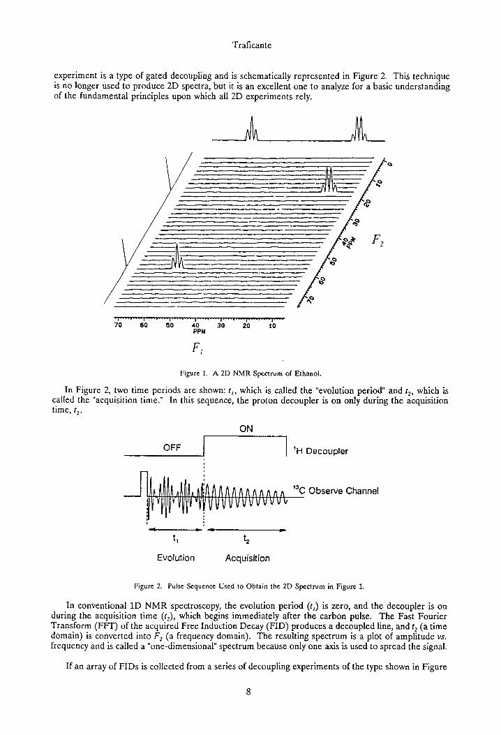
experiment is a type of gated decoupling and is schematically represented in Figure 2. This technique is no longer used to produce 2D spectra, but it is an excellent one to analyze for a basic understanding of the fundamental principles upon which all 2D experiments rely.

Ί 1 1 [ ■ ■ ■ ■ i . . . . | ) [■■. . 70 60 BO 40 30 20 10

PPM

F,

Figure 1. A 2D NMR Spectrum of Ethanol.

In Figure 2, two time periods are shown: t„ which is called the "evolution period" and t2, which is called the "acquisition time." In this sequence, the proton decoupler is on only during the acquisition time, t2.

ON

OFF 'H Decoupler

;.f fwi/wvww "' C Observe Channel

Evolution Acquisition

Figure 2. Pulse Sequence Used to Obtain the 2D Spectrum in Figure 1.

In conventional ID NMR spectroscopy, the evolution period (f;) is zero, and the decoupler is on during the acquisition time (t2), which begins immediately after the carbon pulse. The Fast Fourier Transform (FFT) of the acquired Free Induction Decay (FID) produces a decoupled line, and t2 (a time domain) is converted into F2 (a frequency domain). The resulting spectrum is a plot of amplitude vs. frequency and is called a "one-dimensional" spectrum because only one axis is used to spread the signal.

If an array of FIDs is collected from a series of decoupling experiments of the type shown in Figure

8


2, where t¡ is progressively increased in small steps from zero to a time t, then the FFT of these FIDs will produce a corresponding array of ID spectra. Each of these spectra will be a plot of amplitude (A) vs. F2, and each will be separated from the next by the f, increment used to obtain the individual FIDs. The resulting matrix is a plot of A vs. F2 vs. t¡. If another FFT is performed along t,, point by point along F2, then the t, (a time domain) axis is converted to an F, (a frequency domain) axis, and the final matrix is a plot of A vs. F2 vs. F¡. The result is a two-dimensional spectrum because the signal is then spread along two frequency axes.

In Figure 1, two projections are shown: one onto the F, axis, and one onto the F2 axis. The first projection gives a fully proton-coupled (undecoupled) carbon spectrum, and the second gives a fully proton-decoupled carbon spectrum. Also visible in this 2D spectrum are the multiplicities and carbon-proton coupling constants for each carbon nucleus. These can be obtained from ID "slices" or "cross-sections" that are parallel to F, and taken at the appropriate points along the F2 axis.

A TYPICAL ID SPECTRUM

A more detailed explanation of the production of a 2D spectrum must begin with a complete analysis of a ID experiment. Consider the case of a single carbon nucleus that is coupled to two equivalent protons with a long-range coupling constant of two Hz. Assume that the pulsed transmitter frequency is set to be one Hz lower than the lowest frequency of the triplet. Under these conditions, a ID proton-coupled spectrum will show three lines with intensities 1:2:1 and with frequencies of one, three and five Hz from zero Hz, which is the center of the spectrum when quadrature phase detection is used to acquire the FID. The proton-decoupled spectrum will show a single line located three Hz away from zero Hz, and with a relative intensity of four, neglecting any Nuclear Overhouser Effect (NOE).

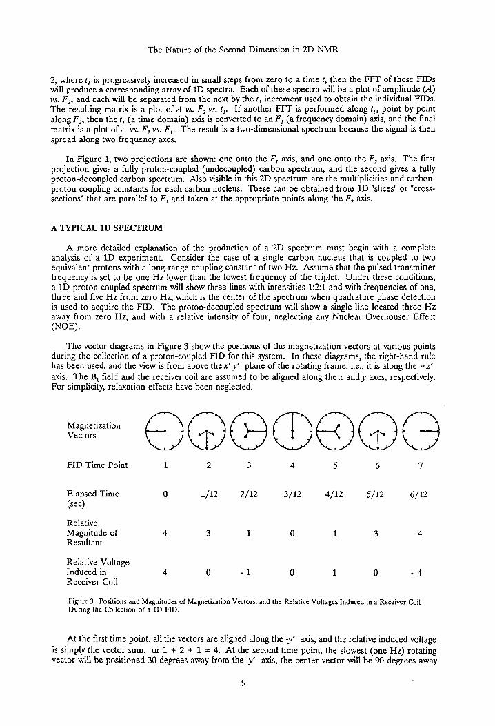
The vector diagrams in Figure 3 show the positions of the magnetization vectors at various points during the collection of a proton-coupled FID for this system. In these diagrams, the right-hand rule has been used, and the view is from above the x' y' plane of the rotating frame, i.e., it is along the +z' axis. The Bj field and the receiver coil are assumed to be aligned along the x and y axes, respectively. For simplicity, relaxation effects have been neglected.

Magnetization Vectors

FID Time Point

Elapsed Time (sec)

Relative Magnitude of Resultant

1/12 2/12 3/12 4/12 5/12 6/12

Relative Voltage Induced in Receiver Coil

- 1 - 4

Figure 3. Positions and Magnitudes of Magnetization Vectors, and the Relative Voltages Induced in a Receiver Coil During the Collection of a ID FID.

At the first time point, all the vectors are aligned Jong the -y' axis, and the relative induced voltage is simply the vector sum, or 1 + 2 + 1 = 4. At the second time point, the slowest (one Hz) rotating vector will be positioned 30 degrees away from the -y' axis, the center vector will be 90 degrees away

9

Traficante

because it rotates at three Hz in the rotating frame, and the fastest (five Hz) vector will be at 150 degrees. The relative voltage induced in the receiver coil is now obtained by first making the vector sum, and then, from this resultant, calculating the component that lies along the y' axis. The same procedure applies to all subsequent time points. The FID produced by these voltages will be similar to the one shown during the t¡ period in Figure 2, and the FFT of this FID will produce a spectrum showing a triplet, with lines at one, three, and five Hz.

The details of how this ID FID is produced are of paramount importance in understanding the second dimension in 2D NMR, and these details will be emphasized again later. The important point to remember is: This FID consists of a sequence of voltages induced by the y' components of the resultants of the three separating vectors.

If this were a ID proton-decoupled experiment, only one vector with a magnitude of four would rotate at a three Hz rate. The relative voltages induced in this case would be 4, 0, -4, 0, 4, 0, -4, at the same time points shown above. The FID produced by these voltages would be similar to the one shown during the t2 period in Figure 2, and the FFT of this FID would produce a spectrum showing a single three Hz line.

THE SECOND DIMENSION IN 2D NMR

The diagrams in Figure 4 show the magnetization vectors, the FIDs, and the resulting real spectra produced at various points in time during the 2D experiment.

Vectors Vectors Vector Sum FID Spectral at Í = 0 í, at f=r, Decoupler On Waveform Lineshupe

Θ JL

1/12

2/12

3/12

^ ^

4/12 L* \ £ _ } ^

5/12

6/12 Θ ^^ Γ\ ΛΓ Figure 4. Positions of Magnetization Vectors, the FIDs, and Real Spectra Obtained During the 2D NMR Experiment Shown in Figure 2.

10


The sequence begins with t¡ = 0 sec, and the t¡ increment is 1/12 second. The first column shows the positions of the net magnetization vectors after the 90-degree pulse. The second column shows the evolution period, t¡, and the third column shows the positions of the individual vectors after the evolution period is complete. Consider now the effect on the system if the decoupler is turned on at time (;. Since we know that only one frequency is collected, the three vectors must not be separating during time t2. If they were separating, three frequencies would be present in the FID, the FFT of which would produce a triplet. It must be remembered that a frequency in an FID is generated from a rotating vector. Hence, three frequencies are generated from three vectors rotating at different rates, and the angles between these vectors will change as time progresses. It follows that if only one frequency is collected during t2, the angles between the three vectors in column 3 must "lock" when the decoupler is turned on, and the entire system must rotate at three Hz, the frequency of the decoupled line. The angles cannot continue to change because this would mean that the vectors are rotating at different rates and would produce more than one frequency in the FID.

Once the system "locks" and rotates at three Hz, it is equivalent to a single vector (i.e., the resultant) rotating at three Hz. The resultants of the vectors shown in column 3 are represented in column 4, and it is these single vectors that produce the FID signals shown in column 5. In this column, only one cycle of the waveform is shown for simplicity.

In column 4, the length (magnitude) and position (phase) of the vector are dependent upon how much the system evolved during t,. Hence, the amplitude and phase, but not the fequency, of the three Hz signal will also depend on the evolution period. The shapes of the resonance lines produced in the real spectra obtained from the FIDs are shown in the last column. The amplitudes and phases of these spectral lines vary in accordance with the lengths and positions of the resultants shown in column 4.

A stacked plot of the spectra in the last column is the matrix described earlier, i.e., a plot of A vs. F2 vs. t,. An example of such a stacked plot is shown in Figure 5, which shows spectra obtained with smaller increments than those shown in Figure 4.

Figure 5. A Stacked Plot of ID Spectra.

11

Traficante

The spectral points at the exact centers of the peaks are also emphasized in this figure. If the magnitudes of these points are plotted as a function of time, specifically, t,, the result will be the same as the FID shown during the t, time in Figure 2.

An explanation for this lies in the fact that columns 3, 4, 5, and 6 in Figure 4 all contain the same information, but presented in different ways. For example, a spectrum in the last column shows that the signal in the frequency domain has the characteristic properties of magnitude, frequency and phase; but, these same three properties are also clearly shown in the time domain signal in column 5, which, in turn, was produced by the rotating vector in column 4. This vector also has a magnitude, phase, and frequency of rotation and is the resultant of the vectors in column 3.

In the discussion of Figure 3, it was explained that the rotating vectors in the first line of that figure gave rise to an FID that produces a triplet after an FFT is performed. At corresponding time points, the vectors in Figure 3 are identical to those in the third column of Figure 4, and if by some method an FFT could be performed on this column, a triplet would also be produced because three vectors are rotating with different frequencies. This can be accomplished by performing the FFT on the center points of the signals in column 6. The magnitudes of these center points are proportional to the y ' components of the resultants of the vectors in column 3. Hence, if the central points of the spectral lines are plotted as a function of the evolution period, t¡, the result would be identical to the FID shown during the t¡ period in Figure 2. That FID was also produced by they' components of the resultants of the three separating vectors. The only difference is that the time domain for the FID in Figure 2 is "real" time, whereas the time domain for the "FID" obtained from the central points of the spectral lines is "virtual" time. This distinction is ignored by the computer while performing an FFT. We, as scientists, think of an FID as a plot of voltage vs. time, but the computer "thinks" of it simply as a one-dimensional array, i.e., unitless magnitude (not voltage) vs. computer word number (not time). Thus, the FFT of the "virtual-time FID" obtained from the central points of the spectral lines would be identical to the one obtained from the "real-time FID" shown in Figure 2; both would be 1:2:1 triplets with a separation of two Hz.

After the FFT is performed along t¡, the resulting 2D matrix is a plot of A vs. F2 vs. F¡ and would have the appearance of Figure 1, except that only one triplet would be visible. For ethanol, two spectral Unes would be visible in column 6 in Figure 4. One of those, the méthylène carbon line, would vary along t, in much the same manner as described above. However, the line from the methyl carbon would vary in a different way because it would be produced from four (instead of three) vectors separating in column 3. Nevertheless, the same general arguments would apply, and an FFT of the central points of this line, as a function t¡, would yield a quartet.

SUMMARY

In a conventional ID experiment involving a coupled-spin system, the instantaneous FID voltage induced in the receiver coil is directly proportional to they' component of the resultant of the rotating magnetization vectors that comprise the transverse components of the system at that instant in time. The FFT of this sequence of voltages collected in "real" time produces a spectrum consisting of a number of lines equal to the number of rotating vectors. In a conventional 2D experiment, a series of ID spectra are obtained as a function of an evolution period, t¡. The magnitude of the central point of a spectral line is directly proportional to the y' component of the resultant of the rotating magnetization vectors at time t¡. Hence, the FFT of this sequence of values obtained in "virtual" time produces a spectrum along the F, axis that consists of a number of lines equal to the number of rotating vectors that give rise to that line. A 2D spectrum is the final result.

ACKNOWLEDGEMENT

The author wishes to acknowledge the efforts of Dr. Michael McGregor, who obtained the spectra for use in this article.

12


REFERENCES

1.) J. Jeener, Ampere International Summer School, Basko Polje, Yugoslavia, 1971.

2.) L. Müller, A. Kumar and R. R. Ernst, 'Two-Dimensional Carbon-13 NMR Spectroscopy,"/. Chem. Phys. 1975, 63, 5490-5491.

13

Documents

The nature of the second dimension in 2D NMR