Embed Size (px)
Citation preview

1st July - 5 thJulyUniversità degli Studi di Milano-Bicocca, Milan, Italy
Logic, Algorithms, ApplicationsThe Nature of Computation
COMPUTABILITYIN EUROPE 2013COMPUTABILITYIN EUROPE 2013
cie2013.disco.unimib.it
Informal Proceedings
2013

Preface
Computability in Europe 2013 (CiE 2013) followed the Turing Centenary Con-ference CiE 2012 in celebrating the enormous influence of Turing’s work on thespecific focus of the CiE conference series: the development of a multi-disciplinaryand modern view of computation and computability. The interest for computa-tion in nature (which was also the motivation for Turing’s work on biologicalpattern formation) as reflected in the title of CiE 2013, The Nature of Com-putation, connects biology and computer science and has given rise to moderndisciplines of research as well as new perspectives on computation.
In particular, CiE 2013 was focused on the unexpected changes that stud-ies on nature have brought to several areas of mathematics, physics, and com-puter science. Two complementary research perspectives pervade the Nature ofComputation theme. One is focused on the understanding of new computationalparadigms, inspired by processes occurring in the biological world and resultingin a deeper and modern understanding of the theory of computation. The otherperspective is on our understanding of how computations really occur in nature,on how we can interact with these computations, and their applications.
CiE 2013 was the ninth meeting in the conference series Computability inEurope organized by the Association CiE. The association promotes the devel-opment of computability-related science, ranging from mathematics, computerscience and applications in various natural and engineering sciences, such asphysics and biology, as well as the promotion of related fields, such as philoso-phy and history of computing. In particular, the conference series successfullybrings together the mathematical, logical and computer sciences communitiesthat are interested in developing computability related topics. This year thisscope was strengthened by the co-location of CiE 2013 with UCNC 2013 (Un-conventional Computation and Natural Computation), with Giancarlo Mauri asthe chair of the programme committee.
The two conferences, CiE 2013 and UCNC 2013, were held at the Universityof Milano-Bicocca in Milan, Italy. They shared one plenary invited talk, givenby Endre Szemeredi (Budapest & Piscataway NJ), winner of the Abel Prize in2012, and two tutorials, one by Grzegorz Rozenberg (Leiden & Boulder CO)and one by Gilles Brassard (Montreal QC). Moreover, some satellite events areorganized around the two conferences.
The eight previous CiE conferences were held in Amsterdam (The Nether-lands) in 2005, Swansea (Wales) in 2006, Siena (Italy) in 2007, Athens (Greece)in 2008, Heidelberg (Germany) in 2009, Ponta Delgada (Portugal) in 2010, Sofia(Bulgaria) in 2011, and Cambridge (England) in 2012. The proceedings of thesemeetings were all published in the Springer series Lecture Notes in ComputerScience. The annual CiE conference has become a major event and is the largestinternational meeting focused on computability theoretic issues. The next meet-ing in 2014 will be held in Budapest (Hungary).
The series is coordinated by the CiE Conference Series Steering Commit-tee consisting of Luıs Antunes (Porto, Secretary), Arnold Beckmann (Swansea),Laurent Bienvenu (Paris), Natasha Jonoska (Tampa FL), Viv Kendon (Leeds),
i

Benedikt Lowe (Amsterdam & Hamburg, chair), Mariya Soskova (Sofia & Berke-ley CA), and Peter van Emde Boas (Amsterdam).
Programme Committee
The Programme Committee of CiE 2013 was responsible for the selection of theinvited speakers, the special session organizers and for running the reviewingprocess of all submitted regular contributions. It consisted of Gerard Alberts(Amsterdam), Luıs Antunes (Porto), Arnold Beckmann (Swansea), Laurent Bi-envenu (Paris), Paola Bonizzoni (Milan, co-chair), Vasco Brattka (Munich &Cape Town, co-chair), Cameron Buckner (Houston TX), Bruno Codenotti (Pisa),Stephen Cook (Toronto ON), Barry Cooper (Leeds), Ann Copestake (Cam-bridge), Erzsebet Csuhaj-Varju (Budapest), Anuj Dawar (Cambridge), GianlucaDella Vedova (Milan), Liesbeth De Mol (Ghent), Jerome Durand-Lose (Orleans),Viv Kendon (Leeds), Bjørn Kjos-Hanssen (Honolulu HI), Antonina Kolokolova(St. John’s NF), Benedikt Lowe (Amsterdam & Hamburg), Giancarlo Mauri(Milan), Rolf Niedermeier (Berlin), Geoffrey Pullum (Providence RI & Edin-burgh), Nicole Schweikardt (Frankfurt), Sonja Smets (Amsterdam), Susan Step-ney (York), S.P. Suresh (Chennai), and Peter van Emde Boas (Amsterdam).
Structure and Programme of the Conference
The programme committee invited six speakers to give plenary lectures: UlleEndriss (Amsterdam), Lance Fortnow (Atlanta GA), Anna Karlin (Seattle WA),Bernard Moret (Lausanne), Mariya Soskova (Sofia & Berkeley CA), and EndreSzemeredi (Budapest & Piscataway NJ; joint invitee of CiE 2013 and UCNC2013).
These plenary speakers were invited to publish abstracts or papers in thisvolume. Karlin’s lecture was the 2013 APAL Lecture funded by Elsevier, Fort-now’s lecture was the 2013 EACSL Lecture funded by the European Associationfor Computer Science Logic, and Szemeredi’s lecture was funded by the Depart-ment of Mathematics and its Applications of the University of Milano-Bicocca.In addition to the plenary lectures, the conference had two tutorials by GillesBrassard (Montreal QC) and Grzegorz Rozenberg (Leiden & Boulder CO).
Springer-Verlag generously funded two awards that were given during the CiE2013 conference. Nicolas de Rugy-Altherre was awarded the Best Student PaperAward for his paper “Determinant versus Permanent: Salvation via Generaliza-tion?” Shankara Narayanan Krishna, Marian Gheorghe, and Ciprian Dragomirwere awarded the Best Paper on Natural Computing Award for their paper “SomeClasses of Generalised Communicating P Systems and Simple Kernel P Sys-tems.”
The conference CiE 2013 had six special sessions: two sessions ComputationalMolecular Biology and Computation in Nature, were devoted to the special fo-cus of CiE 2013. In addition to this, new challenges arising in computationsin the real world were faced in the session on Data Streams and Compression.The remaining three sessions were on Algorithmic Randomness, Computational
ii

Complexity in the Continuous World, and History of Computation. Speakers inthese special sessions were selected by the special session organizers and couldcontribute a paper to this volume.
Algorithmic Randomness.Organizers. Mathieu Hoyrup (Nancy) and Andre Nies (Auckland).Speakers. Johanna Franklin (Storrs CT), Noam Greenberg (Wellington),Joseph S. Miller (Madison WI), Nikolay Vereshchagin (Moscow).
Computational Complexity in the Continuous World.Organizers. Akitoshi Kawamura (Tokyo) and Robert Rettinger (Hagen).Speakers. Mark Braverman (Princeton NJ), Daniel S. Graca (Faro), Jorisvan der Hoeven (Palaiseau), Chee K. Yap (New York NY).
Computational Molecular Biology.Organizers. Alessandra Carbone (Paris) and Jens Stoye (Bielefeld).Speakers. Sebastian Bocker (Jena), Marılia D.V. Braga (Duque de Caxias),Andrea Pagnani (Torino), Laxmi Parida (Yorktown Heights NY).
Computation in Nature.Organizers. Mark Delay (London ON) and Natasha Jonoska (Tampa FL).Speakers. Jerome Durand-Lose (Orleans), Giuditta Franco (Verona), LilaKari (London ON), Darko Stefanovic (Albuquerque NM).
Data Streams and Compression.Organizers. Paolo Ferragina (Pisa) and Andrew McGregor (Amherst MA).Speakers. Graham Cormode (Florham Park NJ), Irene Finocchi (Rome),Andrew McGregor (Amherst MA), Marinella Sciortino (Palermo).
History of Computation.Organizers. Gerard Alberts (Amsterdam) and Liesbeth De Mol (Ghent).Speakers. David Alan Grier (Washington DC), Thomas Haigh (MilwaukeeWI), Ulf Hashagen (Munich), Matti Tedre (Stockholm).
All authors who have contributed to this conference are encouraged to submitsignificantly extended versions of their papers with unpublished research contentto Computability. The Journal of the Association CiE.
Organisation and Acknowledgements.
The conference CiE 2013 was organised by Stefano Beretta (Milan), Paola Boniz-zoni (Milan), Gianluca Della Vedova (Milan), Alberto Dennunzio (Milan), Ric-cardo Dondi (Bergamo), Giancarlo Mauri (Milan), Yuri Pirola (Milan) and Raf-faella Rizzi (Milan).
The Steering Committee of the conference series CiE is concerned about therepresentation of female researchers in the field of computability. In order toincrease female participation, the series started the Women in Computability(WiC) programme in 2007, first funded by the Elsevier Foundation, then takenover by the publisher Elsevier. We were proud to continue this programme withits successful annual WiC workshop and a grant programme for junior femaleresearchers in 2013.
iii

The organizers of CiE 2013 would like to acknowledge and thank the followingentities for their essential financial support (in alphabetic order): the Associa-tion for Symbolic Logic (ASL), the Department of Mathematics and its Appli-cations and the Department of Informatics, Systems and Communication, bothof the University of Milano-Bicocca, Elsevier B.V., the European Associationfor Computer Science Logic (EACSL), the European Association for Theoreti-cal Computer Science (EATCS), IOS Press, Springer-Verlag and the Universityof Milano-Bicocca. We would also like to acknowledge the support of our non-financial sponsors, the Association Computability in Europe (CiE).
June 11, 2013Milano
Paola BonizzoniVasco Brattka
Gianluca Della VedovaBenedikt Lowe
iv

Table of Contents
Efficient Computation of the Gap-Weighted Subsequence Kernel . . . . . . . . 1Slimane Bellaouar, Hadda Cherroun and Djelloul Ziadi
Reaction systems with constrained environment . . . . . . . . . . . . . . . . . . . . . . . 11Paolo Bottoni and Anna Labella
The Nature of Computation and The Development of ComputationalModels . . . . . . . . . . . . . . . . . . . . . . . . . . . . . . . . . . . . . . . . . . . . . . . . . . . . . . . . . . 21
Mark Burgin and Gordana Dodig Crnkovic
Towards a Church-Turing-Thesis for Infinitary Computations . . . . . . . . . . . 30Merlin Carl
The Bottleneck Selected-Internal Steiner Tree Problem: Hardness andApproximation . . . . . . . . . . . . . . . . . . . . . . . . . . . . . . . . . . . . . . . . . . . . . . . . . . . 40
Yen Hung Chen
A History of Autonomous Agents: from Thinking Machines to Machinesfor Thinking . . . . . . . . . . . . . . . . . . . . . . . . . . . . . . . . . . . . . . . . . . . . . . . . . . . . . 50
Stefania Costantini and Federico Gobbo
Brute Force is not Ignorance . . . . . . . . . . . . . . . . . . . . . . . . . . . . . . . . . . . . . . . 60Joseph Davidson and Greg Michaelson
An Extended Fundamental Duality of Partially Ordered Sets and ItsApplications . . . . . . . . . . . . . . . . . . . . . . . . . . . . . . . . . . . . . . . . . . . . . . . . . . . . . . 70
Mustafa Demirci
RNA pseudoknot prediction through stochastic conjunctive grammars . . . 80Mike Domaratzki and Ryan Zier-Vogel
A Kripke Model for Subrecursion. . . . . . . . . . . . . . . . . . . . . . . . . . . . . . . . . . . . 90Joaquın Dıaz Boils and Jose Pedro Ubeda Rives
How to reduce backtracking in propositional intuitionistic logic . . . . . . . . . 100Guido Fiorino
Graphs realised by r.e. equivalence relations . . . . . . . . . . . . . . . . . . . . . . . . . . 110Alexander Gavruskin, Sanjay Jain, Bakhadyr Khoussainov and FrankStephan
A Unifying Approach to Decide Timed Relations for Timed Automataand their Game Characterization . . . . . . . . . . . . . . . . . . . . . . . . . . . . . . . . . . . 120
Shibashis Guha, Krishna S, Chinmay Narayan and S. Arun-Kumar
Vector Addition Systems With Split/Join Transitions: A CoveringTheorem . . . . . . . . . . . . . . . . . . . . . . . . . . . . . . . . . . . . . . . . . . . . . . . . . . . . . . . . . 131
Paulin Jacobe De Naurois
v

Lowness for uniform Kurtz randomness . . . . . . . . . . . . . . . . . . . . . . . . . . . . . . 141Takayuki Kihara and Kenshi Miyabe
A Species Distribution Framework Relying on Membrane Computingwith Boundaries . . . . . . . . . . . . . . . . . . . . . . . . . . . . . . . . . . . . . . . . . . . . . . . . . . 151
Tamas Mihalydeak and Zoltan Erno Csajbok
Undecidability of satisfiability of expansion of FO[<] with a SemilinearNon Regular Predicate over words. . . . . . . . . . . . . . . . . . . . . . . . . . . . . . . . . . . 161
Arthur Milchior
Passive Computation and the Power of Inactivity: How to Get a Brainto Compute without Firing its Neurons . . . . . . . . . . . . . . . . . . . . . . . . . . . . . 171
Bernard Molyneux
Formal Philosophy and Legal Reasoning: The validity of legal inferences . 181Clayton Peterson
A Memetic Algorithm for Solving the Generalized Vehicle RoutingProblem . . . . . . . . . . . . . . . . . . . . . . . . . . . . . . . . . . . . . . . . . . . . . . . . . . . . . . . . . 201
Petrica Pop and Oliviu Matei
A Modal Type System for Error Handling . . . . . . . . . . . . . . . . . . . . . . . . . . . . 211Giuseppe Primiero
The double negation translation in Nonstandard Constructive Analysis . . 221Sam Sanders
Decidability and the multiplicative structure of positive rationalstogether with the ‘greatest common divisor’ . . . . . . . . . . . . . . . . . . . . . . . . . . 236
Alla Sirokofskich
Formal Representations of Pronouns Using Universal Networking Language 245Velislava Stoykova
The d-distance anticoloring Problem . . . . . . . . . . . . . . . . . . . . . . . . . . . . . . . . . 251Shira Zucker
vi

Program Committee
Gerard Alberts University of AmsterdamLuıs Antunes Computer Science Dep., University of PortoArnold Beckmann Swansea UniversityLaurent Bienvenu LIAFAPaola Bonizzoni universit di Milano-BicoccaVasco Brattka University of Cape TownCameron Buckner UHBruno Codenotti CNRStephen Cook University of TorontoS. Barry Cooper University of LeedsAnn Copestake University of CambridgeErzsebet Csuhaj-Varju Computer and Automation Research Institute, Hun-
garian Academy of SciencesAnuj Dawar University of CambridgeLiesbeth De Mol Universiteit GentGianluca Della Vedova Dipartimento di Statistica, Univ. degli Studi Milano-
BicoccaJerome Durand-Lose LIFO - U. D’OrleansViv Kendon School of Physics and Astronomy, University of
LeedsBjoern Kjos-Hanssen University of Hawai’iAntonina Kolokolova Memorial University of NewfoundlandBenedikt Lowe Universiteit van AmsterdamGiancarlo Mauri University of Milano-BicoccaRolf Niedermeier TU BerlinGeoffrey K. Pullum University of EdinburghNicole Schweikardt Univ. FrankfurtSonja Smets Universiteit GroningenSusan Stepney York UniversityS P Suresh Chennai Mathematical InstitutePeter Van Emde Boas ILLC-FNWI-Universiteit van Amsterdam (emeri-
tus)
vii

Additional Reviewers
AAbu Zaid, FariedAizawa, KennethAllo, PatrickAlmeida, MarcoAman, BogdanAnderson, MatthewAndrews, PaulArkhipov, AlexArrighi, PabloBBadillo, LilianaBarmpalias, GeorgeBarr, KatieBauer, AndrejBauwens, BrunoBernardinello, LucaBesozzi, DanielaBlock, AlexanderBonfante, GuillaumeBraverman, MarkBredereck, RobertBrenguier, RomainBridges, DouglasBrijder, RobertBriseid, EyvindBulteau, LaurentBes, AlexisCCalvert, WesleyCaravagna, GiulioCarl, MerlinCarlucci, LorenzoCarton, OlivierCase, JohnChen, JiehuaChivers, HowardColombo, RiccardoCormode, GrahamCorreia, LuisDDahmani, Francois
viii

De Paiva, ValeriaDelhomme, ChristianDennunzio, AlbertoDiener, HannesDondi, RiccardoDorais, FrancoisDowek, GillesDroop, AlastairDyckhoff, RoyEEckert, KaiEguchi, NaohiEscardo, MartinFFerretti, ClaudioFinkel And Christoph Haase, AlainFiorino, GuidoFisseni, BernhardFokina, EkaterinaFranco, GiudittaFranklin, Johanna N.Y.Franks, DanFraser, RobertFreer, CameronFrehse, GoranFriedman, Sy-DavidFroese, VincentGGacs, PeterGagie, TravisGheorghe, MarianGherardi, GuidoGhosh, S.Gierasimczuk, NinaGivors, FabienGoldberg, PaulGoubault-Larrecq, JeanGutierrez-Naranjo, Miguel AGartner, BerndGorecki, PawelHHansen, Jens UlrikHarizanov, ValentinaHartung, SeppHertling, Peter
ix

Heunen, ChrisHickinbotham, SimonHines, PeterHirschfeldt, DenisHoyrup, MathieuHutter And Wen Shao, MarcusHolzl, RupertHuffner, FalkIInamdar, TanmayIvan, SzabolcsKKabanets, ValentineKalimullin, IskanderKari, JarkkoKari, LilaKato, YukiKawamura, AkitoshiKent, TomKihara, TakayukiKishida, KoheiKleijn, JettyKlincewicz, MichalKolde, RaivoKomusiewicz, ChristianKullmann, OliverLLange, KarenLazic, RankoLe Gloannec, BastienLeal, RaulLeporati, AlbertoLi, ZhenhaoLoeb, IrisLovett, NeilMMalcher, AndreasManea, FlorinManzoni, LucaMargenstern, MauriceMarks, AndrewMartiel, SimonMartini, SimoneMaurino, AndreaMichaelson, Greg
x

Miller, RussellMontalban, AntonioMoore, CrisMorozov, AndreiMota, FranciscoMummert, CarlNNguyen, NamNguyen, PaulNichterlein, AndreNies, AndreNobile, MarcoNoessner, JanNordvall Forsberg, FredrikOO’Keefe, SimonOkhotin, AlexanderPPanangaden, PrakashPaun, GheorghePavesi, GiulioPescini, DarioPike, DavidPirola, YuriPorreca, AntonioPoulding, SimonPouly, AmauryPrimiero, GiuseppePuzarenko, VadimRRizzi, RaffaellaRomashchenko, AndreiRothe, JrgRussell, BenjaminRute, JasonSSalomaa, Kai T.Sampson, AdamSan Mauro, LucaSankur, OcanSapir, MarkSavani, RahulSciortino, MarinellaSeisenberger, MonikaSeki, Shinnosuke
xi

Sequoiah-Grayson, SSergioli, GiuseppeSeyfferth, BenjaminShafer, PaulShen, AlexanderShen, SashaShlapentokh, AlexandraSimmons, HaroldSimon, Sunil EasawSimonnet, PierreSkordev, DimiterSolomon, ReedSorbi, AndreaSorge, ManuelSoskova, AlexandraSourabh, SumitSouto, AndreSprevak, MarkStamatiou, YannisStannett, MikeSteffen, BernhardStephan, FrankSuchy, OndraSzymanik, JakubTThierauf, ThomasThomson And Rajeev Gore, JimmyTsigaridas, EliasUUckelman, JoelVvan Bevern, Renevan Den Berg, BennoVatev, StefanVerlan, SergeyVicary, JamieWWareham, ToddWeihrauch, KlausWeller, MathiasYYakoubsohn, Jean-ClaudeYokoyama, KeitaZZandron, Claudio
xii

Ziegler, MartinZoppis, Italo
xiii

Efficient Computation of the Gap-WeightedSubsequence Kernel?
Slimane Bellaouar1, Hadda Cherroun1, and Djelloul Ziadi2
1 Laboratoire LIM, Université Amar Telidji, Laghouat, Algéries.bellaouar,[email protected]
2 Laboratoire LITIS - EA 4108, Université de Rouen, Rouen, [email protected]
Abstract. In this paper, we present a novel approach to compute effi-ciently the gap weighted subsequence kernel (GWSK). We have startedby the construction of a match list L(s, t) = (i, j) : si = tj where s andt are the strings to be compared. Then, we have constructed a layeredrange tree and a list of lists. The whole process takes O(|L| log |L|+ pK)time and O(|L| log |L|+K) space, where |L| is the size of the match list,p is the length of the GWSK and K is the total reported points by rangequeries over all the entries of the match list.
Keywords: string kernel, computational geometry, layered range tree,range query
1 Introduction
Kernel methods [1] were proposed as an alternative solution to the limitation oftraditional machine learning algorithms applied, solely, on linear separable prob-lems. They project the data into a high dimensional feature space where linearlearning machines based on algebra, geometry and statistics can be applied.Hence, non-linear relations can be discovered. Moreover, the kernel methodsenables other types of data (biosequences, images, graphs, . . . ) to be processed.
Strings are considered among the important data types. Therefore, a greateffort of research has been devoted to string kernels that are widely used in thefields of bioinformatics and natural language processing. The philosophy of allstring kernels can be reduced to different ways to count common substrings orsubsequences that occur in the two strings to compare, say s and t.
There are two main approaches to improve the computation of the gap-weighted subsequence kernel (GWSK). The first one is based on dynamic pro-gramming paradigm; Lodhi et al. [2] have applied dynamic programming paradigmto the suffix version of the GWSK. Later, Rousu and Shawe-Taylor [3] have pro-posed an improvement to the dynamic programming approach. They have useda set of match lists combined with a sum range tree. The trie-based approach [4]
? This work is supported by the MESRS - Algeria under Project 8/U03/7015.
1

is based on depth first traversal on an implicit trie data structure. The numberof gaps is restricted, so the computation is approximate.
Motivated by the efficiency of the computation, a key property of the kernelmethods, in this paper, we will focus on improving the GWSK computation. Webegin by the construction of a match list L(s, t) = (i, j) : si = tj that containsonly the required data to the computation. The main idea is that the GWSKcomputation corresponds to 2-dimensional range queries on a layered range tree(a range tree enhanced by the fractional cascading technique). The final datastructure built is a list of lists. The overall time complexity is O(|L| log |L|+pK),where |L| is the size of the match list and K is the total reported points by rangequeries over all the entries of the match list.
The rest of this paper is organized as follows. Section 2 deals with someconcept definitions used in the other sections. In section 3, we recall formallythe GWSK computation. We review three efficient computations of the GWSK,namely, dynamic programming, trie-based and sparse dynamic programmingapproaches. Section 4 is devoted to the presentation of our contribution. Section 5includes conclusions and discussion.
2 Preliminaries
This section deals with required concepts to understand the rest of this paper.Let Σ be an alphabet of a finite set of symbols. The number of symbols in Σis denoted by |Σ|. |s| denotes the length of the string s. Σn denotes the set ofall finite strings of length n, and Σ∗ denotes the set of all strings. The notation[s = t] is a boolean function that returns
1 if s and t are identical;0 otherwise.
The ith element of the word s is denoted by si. The string s(i : j) denotesthe substring sisi+1...sj of s. Accordingly, the string t is a substring of a strings if there are strings u and v such that s = utv (u and v can be empty). Thesubstrings of length n are referred to as n-grams (or n-mers).
The string t is a subsequence of s if there exists an increasing sequence ofindices I = (i1, ..., i|t|) in s, (1 ≤ i1 < ... < i|t| ≤ |s|) such that tj = sij , forj = 1, ..., |t|. In the literature, we use t = s(I) if t is a subsequence of s inthe positions given by I. The empty string ε is indexed by the empty tuple. Thelength of the subsequence t is denoted by |t| = |I| which is the number of indices,while l(I) = i|t| − i1 + 1 refers to the number of characters of s covered by thesubsequence t.
3 Gap-Weighted Subsequence Kernels
The GWSK adopts a new weighting method that reflects the degree of contiguityof a subsequence in the string. In order to measure the distance of non contiguous
2
elements of the subsequence, a gap penalty λ ∈]0, 1] is introduced. Formally, themapping function φp(s) in the feature space F can be defined as follows:
φpu(s) =∑
I:u=s(I)
λl(I), u ∈ Σp.
The associated kernel can be written as:
Kp(s, t) = 〈φp(s), φp(t)〉 =∑
u∈Σp
∑
I:u=s(I)
∑
J:u=t(J)
λl(I)+l(J).
A suffix kernel is defined to assist in the computation of the GWSK. The asso-ciated embedding is given by:
φp,Su (s) =∑
I∈I|s|p :u=s(I)
λl(I), u ∈ Σp,
where Ikp denotes the set of p-tuples of indices I with ip = k (see Section 2).The associated kernel can be defined as follows:
KSp (s, t) = 〈φp,S(s), φp,S(t)〉
=∑
u∈Σp
φp,Su (s).φp,Su (t).
The GWSK can be expressed in terms of its suffix version as follows:
Kp(s, t) =
|s|∑
i=1
|t|∑
j=1
KSp (s(1 : i), t(1 : j)), (1)
with KS1 (s, t) = [s|s| = t|t|] λ2.
3.1 Naive Implementation
The computation of the similarity of two strings (sa and tb) is conditioned bytheir final symbols. In the case where a = b, we have to sum kernels of all prefixesof s and t. Hence, a recursion has to be devised:
KSp (sa, tb) = [a = b]
|s|∑
i=1
|t|∑
j=1
λ2+|s|−i+|t|−jKSp−1(s(1 : i), t(1 : j)). (2)
The computation of equation (2) leads to a complexity of O(p(|s|2|t|2)).
3.2 Efficient Implementations
We will present three methods that compute the GWSK efficiently. The firstis based on a dynamic programming approach [2], the second is the trie-basedmethod [4] and the third is a sparse dynamic programming based approach [3].
3

Dynamic Programming Approach. The starting point of the dynamic pro-gramming approach is the suffix recursion given in equation (2). From this equa-tion, we can consider a separate dynamic programming table DPp for storingthe double sum:
DPp(k, l) =
k∑
i=1
l∑
j=1
λk−i+l−j KSp−1(s(1 : i), t(1 : j)). (3)
It is easy to observe that: KSp (sa, tb) = [a = b]λ2DPp(|s|, |t|)).
Computing ordinary DPp for each (k, l) would be inefficient. So we can devise arecursive version of equation (3) with a simple counting device:
DPp(k, l) = KSp−1(s(1 : k), t(1 : l)) + λDPp(k − 1, l) +
λDPp(k, l − 1)− λ2DPp(k − 1, l − 1).
Consequently, the complexity of the GWSK is O(p |s||t|).
Trie-based Approach. This approach is based on search trees known as tries,introduced by E. Fredkin in 1960. The key idea of the trie-based approach isthat leaves play the role of the feature space indexed by the set Σp. In theliterature, there exists a variant of trie-based gap weighted subsequence kernels.For instance the (p,m)-mismatch string kernel [4] and restricted GWSK [5].
In the present section, we try to describe a trie-based GWSK presented in[3] that slightly differ from the one cited above [5]. Given that each node inthe trie corresponds to a co-occurrence between strings, the algorithm stores allmatches s(I) = u1 · · ·uq, I = i1 · · · iq in such node. In parallel, it will maintaina list of alive matches Ls(u, g) that records the last index iq (g is the numberof gaps in the match). Notice that in the same list we are able to record manyoccurrences with different gaps. Similarly, the algorithm is applied to the stringt. The process will continue until achieving the depth p where the kernel will beevaluated as follows:
Kp(s, t) =∑
u∈Σp
φpu(s)φpu(t) =
∑
u∈Σp
∑
gs,gt
λgs+p|Ls(u, gs)| · λgt+p|Lt(u, gt)|.
Given that, there exists(p+mm
)different entries at leaf nodes, the worst-case time
complexity of the algorithm is O((p+mm
)(|s|+ |t|)).
Sparse Dynamic Programming Approach. This approach is built on thefact that in many cases, most of the entries of the DP matrix are zero anddo not contribute on the result. Rousu and Shawe-Taylor [3] have proposed asolution using two data structures. The first one is a set of match lists insteadof the KS
p matrix. The second one is a range sum tree, which is a B-tree, thatreplaces the DPp matrix. It is used to return the sum of n values within aninterval in O(log n) time. Their algorithm runs in O(p|L| logmin(|s|, |t|)), whereL = (i, j)|si = tj.
4

4 List and Layered Range Tree based Approach
Looking forward to improving the complexity of GWSK, our approach is basedon two observations. The first one concerns the computation of KS
p (s, t) that isrequired only when s|s| = t|t|. Hence, we have kept only a list of index pairs ofthese entries rather than the entire suffix table, L(s, t) = (i, j) : si = tj. If weconsider the example which computes Kp(gatta, cata), the list generated is
L(gatta, cata) = (2, 2), (5, 2), (3, 3), (4, 3), (2, 4), (5, 4).
In the rest of the paper, while measuring the complexity of different compu-tations, we will consider, |L|, the size of the match list L(s, t) as the parameterindicating the size of the input data.
The complexity of the naive implementation of the list version is O(p|L|2),and it seems not obvious to compute KS
p (s, t) efficiently on a list data structure.In order to address this problem, we have made a second observation that thesuffix table can be represented as a two-dimensional space (plane) and the entrieswhere s|i| = t|j| as points in this plane.
At the light of this observation, the computation of KSp (s, t) can be inter-
preted as an orthogonal range query. In the literature, there exist several datastructures that are used in computational geometry. We have examined a spa-tial data structure known as Kd-tree [6, 7, 8]. It records a total time cost ofO(p(|L|
√|L| + K)) for computing the GWSK, where K is the total of the re-
ported points. It is clear that this relative amelioration is not sufficiently satisfac-tory. So we adopted another spatial data structure, called range tree [7, 8, 9, 10],which has better query time for rectangular range queries. We will describe suchdata structure and its relationship with GWSK in the following sub sections.
4.1 Suffix Table Representation
The entries (k, l) in L(s, t) correspond to a set S of points in the plane, wherethe index pairs (k, l) play the role of the point coordinates. The set S is rep-resented by a 2-dimensional range tree, where nodes represent points in theplane. Thereby, representing the suffix table tend to be the construction of a2-dimensional range tree. A range tree, denoted by RT is primarily a balancedbinary search tree (BBST) augmented with an associated data structure. Inorder to build such data structure, first, we consider the set Sx of the first co-ordinate (x-coordinate) values of all the points in S. Thereafter, a BBST calledx-RT is constructed with points of Sx in the leaves. Both internal or leaf nodesv of x-RT are augmented by a 1-dimensional range tree, it can be a BBST ora sorted array, of a canonical subset P (v) on y-coordinates, denoted by y-RT .The subset P (v) is the points stored in the leaves of the sub tree rooted at thenode v. Figure 1 illustrates the construction process of a 2-dimensional rangetree.
In the case where two points have the same x or y-coordinate, we have todefine a total order by using a lexicographic one. It consists to replace the real
5

Fig. 1. Layered range tree RT related to KSp (gatta, cata)
number by a composite-number space [7]. The composite number of two reals xand y is denoted by x|y, so for two points, we have:
(x|y) < (x′|y′)⇔ x < x′ ∨ (x = x′ ∧ y < y′).
In such situation, we have to transform the range query [x1 : x2] × [y1 : y2]related to a set of points in the plane to the range query [(x1| − ∞) : (x2| +∞)]× [(y1| −∞) : (y2|+∞)] related to the composite space.
Based on the algorithm analysis of computational geometry algorithms, our2-dimensional range tree requires O(|L| log |L|) storage and can be constructedin O(|L| log |L|) time. This leads to the following lemma.
Lemma 1. Let s and t be two strings and L(s, t) = (i, j) : si = tj the matchlist associated to the suffix version of the GWSK. A range tree for L(s, t) requiresO(|L| log |L|) storage and takes O(|L| log |L|) construction time.
4.2 Location of Points in a Range
We recall that computing the recursion for the GWSK given by the equation(2) can be interpreted as the evaluation of a 2-dimensional range query appliedto a 2-dimensional range tree. Such evaluation locates all points that lie in thespecified range.
A useful idea, in terms of efficiency, consists on treating a rectangular rangequery as a two nested 1-dimensional queries. In other words, let [x1 : x2]×[y1 : y2]be a 2-dimensional range query, we first ask for the points with x-coordinates inthe given 1-dimensional range query [x1 : x2]. Consequently, we select a collectionof O(log |L|) subtrees. We consider only the canonical subset of the resulted
6

subtrees, which contains, exactly, the points that lies in the x-range [x1 : x2]. Atthe next step, we will only consider the points that fall in the y-range [y1 : y2].The total task of a range query can be performed in O(log2 |L|+ k) time, wherek is the number of points that are in the range. We can improve it by enhancingthe 2-dimensional range tree with the fractional cascading technique which isdescribed in the following subsection.
4.3 Fractional Cascading
The key observation made during the invocation of a rectangular range query isthat we have to search the same range [y1 : y2] in the associated structures y-RT of O(log |L|) nodes found while querying the x-RT by the range query [x1 :x2]. Moreover, there exists an inclusion relationship between these associatedstructures. The goal of the fractional cascading consists on executing the binarysearch only once and use the result to speed up other searches without expandingthe storage by more than a constant factor.
The application of the fractional cascading technique introduced by [11] ona range tree creates a new data structure so called layered range tree. We willillustrate such technique through a simple of GWSK computing in Fig. 1.
Using this technique, the rectangular search query time becomes O(log(|L|+k), where k is the number of reported points. For the computation of KS
p (s, t)we have to consider |L| entries of the match list. The process iterates p times,therefore, we get a time complexity of O(p|L| log |L| + K) for evaluating theGWSK, where K is the total of reported points over all the entries of L(s, t).This result combined to that of Lemma. 1 lead to the following Lemma:
Lemma 2. Let s and t be two strings and L(s, t) = (i, j) : si = tj the matchlist associated to the suffix version of the GWSK. A layered range tree for L(s, t)uses O(|L| log |L|) storage and it can be constructed in O(|L| log |L|) time. Withthis layered range tree, the GWSK of length p can be computed in O(p(|L| log |L|+K)), where K is the total number of reported points over all the entries of L(s, t).
4.4 List of lists Building and GWSK Computation
Another observation leads us to pursue our line of reasoning about the improve-ment of the GWSK computation complexity. It is obvious to state that pointcoordinates, in our case, in the plane remain unchanged during the entire pro-cessing. So instead of invoking the 2-dimensional range query multiple timesaccording to the evolution of the parameter p, it is more beneficial if we do thecomputation only once. Accordingly, in this phase, we extend our match list tobe a list of lists (Fig. 2), where each entry (k, l) points to a list that containsall the points that lie in the corresponding range. Algorithm 1 builds this listof lists. The complexity of the construction of the list of lists is the complexityof invoking the 2-dimensional range query over all the entries of the match list.This leads to O(|L| log |L|+K) time complexity.
7

Algorithm 1 List of Lists CreationRequire: match list L(s, t) and Layered Range Tree RT
for each entry (k, l) ∈ L(s, t) doPreparing the range queryx1 ← 0y1 ← 0x2 ← k − 1y2 ← l − 1relatedpoints ← 2D-RANGE-QUERY(RT , [(x1| −∞) : (x2|+∞)]× [(y1| −∞) :(y2|+∞)]while There exists (i, j) ∈ relatedpoints do
add (i, j) to (k, l)-listend while
end forEnsure: List of Lists LL(s, t): The match list augmented with lists containing reportedpoints
Fig. 2. List of lists inherent to KS1 (gatta,cata).
Once the list of lists constructed, the GWSK computation will sum over allthe reported points stored on it. The process is described in Algorithm 2. Thecost of this computation is O(K). Since we will evaluate the GWSK for p ∈[1..min(|s|, |t|)], this leads to a complexity of O(pK). So the over all complexityis O(|L| log |L| + pK) which include the construction of the list of lists and thecomputation of GWSK in the strict sense. This leads to the following theoremthat summarizes the result for the computation of the GWSK.
Theorem 1. Let s and t be two strings and L(s, t) = (i, j) : si = tj the matchlist associated to the suffix version of the GWSK. A layered range tree and a listof lists for L(s, t) require O(|L| log |L|+K) storage and they can be constructedin O(|L| log |L| + K) time. With these data structures, the GWSK of length p
8

can be computed in O(|L| log |L|+ pK), where K is the total number of reportedpoints over all the entries of L(s, t).
Algorithm 2 GWSK computationRequire: List of Lists LL(s, t), subsequence length p and penalty coefficient λ
for q=1:p doInitializationK(q)← 0KPS(1 : |max|)← 0for each entry (k, l) ∈ LL(s, t) do
for each entry r ∈ (k, l)− list do(i, j)← r.KeyKPS(i,j) ← r.V alueKPS(k, l)← KPS(k, l) + λk−i+l−j KPS(i,j)
end forK(q)← K(q) +KPS(k, l))
end forPreparing LL(s, t) For the next computationfor each entry (k, l) ∈ KPS do
Update LL(k, l) with KPS(k, l)end for
end forEnsure: Kernel values Kq(s, t) = K(q) : q = 1, . . . , p
5 Conclusion
We presented a novel algorithm that efficiently computes the gap weighted sub-sequence kernel (GWSK). Our approach is refined over three phases. We beginby the construction of a match list L(s, t) that contains, only, the informationthat contributes in the result. In order to locate, efficiently, the related positionsfor each entry of the match list, we have constructed a layered range tree. Atlast, we have built a list of lists to compute efficiently the GWSK. The Wholetask takes O(|L| log |L|+ pK) time and O(|L| log |L|+K) space, where p is thelength of the GWSK and K is the total number of reported points.
The reached result gives evidence of an asymptotic complexity improvementcompared to that of a naive implementation of the list version O(p |L|2). On theother hand, our intermediate data structure, the layered range tree is outputsensitive. It means that our computation implies, only, required data. However,this dictates to conduct empirical analysis to compare our contribution to otherapproaches. This will be the subject of a future research.
Nevertheless, based on the asymptotic complexities of the different approachesand the experiments presented in [3], we make some discussions. The dynamicprogramming approach is faster when the DPp table is nearly full. This caseis achieved on short strings and on long strings if the alphabet is small. The
9

trie-based approach is faster on medium-sized alphabets but it suffers from gaplength restriction. Furthermore, recall that our approach and the sparse dynamicprogramming one are proposed in the context where the most of the entries ofthe DPp table are zero. This case occurred for large-sized alphabets. From theasymptotic complexity of the sparse approach, O(p|L| logmin(|s|, |t|)), it is clearthat its efficiency depends on the size of the strings. For our approach it dependsonly on the number of common subsequences. Under these conditions our ap-proach outperforms for long strings. Theses discussions will be validated by afuture empirical study.
A noteworthy advantage is that our approach separates the process of re-quired data location from the strict computation one. This separation limits theimpact of the length of the GWSK on the computation. It have influence, only,on the strict computation process. Moreover, such separation property can befavorable if we assume that the problem is multi-dimensional, e.g. comparingseveral strings in the same time. In terms of complexity, this can have influence,only, on the location process by a logarithmic factor. Indeed, the layered rangetree can report points that lies in a rectangular range query in O(logd−1 |L|+k),in a d-dimensional space. At the implementation level, great programming effortis supported by well-studied and ready to use computational geometry algo-rithms. Hence, the emphasis is shifted to a variant of string kernel computationsthat can be easily adapted.
References[1] Cristianini, N., Shawe-Taylor, J.: An introduction to support Vector Machines:
and other kernel-based learning methods. Cambridge University Press, New York,NY, USA (2000)
[2] Lodhi, H., Saunders, C., Shawe-Taylor, J., Cristianini, N., Watkins, C.: Textclassification using string kernels. J. Mach. Learn. Res. 2 (March 2002) 419–444
[3] Rousu, J., Shawe-Taylor, J.: Efficient computation of gapped substring kernels onlarge alphabets. J. Mach. Learn. Res. 6 (December 2005) 1323–1344
[4] Leslie, C., Eskin, E., Noble, W.: Mismatch String Kernels for SVM Protein Clas-sification. In: Neural Information Processing Systems 15. (2003) 1441–1448
[5] Shawe-Taylor, J., Cristianini, N.: Kernel Methods for Pattern Analysis. Cam-bridge University Press, New York, NY, USA (2004)
[6] Bentley, J.L.: Multidimensional binary search trees used for associative searching.Commun. ACM 18(9) (September 1975) 509–517
[7] Berg, M.d., Cheong, O., Kreveld, M.v., Overmars, M.: Computational Geometry:Algorithms and Applications. 3rd ed. edn. Springer-Verlag TELOS, Santa Clara,CA, USA (2008)
[8] Samet, H.: The design and analysis of spatial data structures. Addison-WesleyLongman Publishing Co., Inc., Boston, MA, USA (1990)
[9] Bentley, J.L.: Decomposable searching problems. Inf. Process. Lett. 8(5) (1979)244–251
[10] Bentley, J.L., Maurer, H.A.: Efficient Worst-Case Data Structures for RangeSearching. Acta Informatica 13 (1980) 155–168
[11] Chazelle, B., Guibas, L.J.: Fractional cascading: I. a data structuring technique.Algorithmica 1(2) (1986) 133–162
10

Reaction systems with constrained environment
Paolo Bottoni1 and Anna Labella1
Universita di Roma “Sapienza” (Italy) (bottoni,labella)@di.uniroma1.it
Abstract. Reaction systems model living organisms as systems sustain-ing themselves through reaction processes and receiving contributionsfrom the environment. In the classical model, the system is completelyopen and the environment is completely unpredictable, contributing tosystem evolution via a set-theoretic union operation. We discuss variantsin which the environment can be modeled as a function or relation involv-ing the state of the system and in which communication occurs throughspecific channels. Moreover, we discuss models of environment contribu-tion via intersection and symmetrical difference, rather than union.
1 Introduction
Reaction systems [6], a novel paradigm of nature-inspired computing, model liv-ing organisms by defining self-sustainable sets of reactions which can take placeinside of them. In particular, a reaction can occur if the system’s current config-uration: (1) contains all the reactants needed for it, and (2) does not contain anyinhibitor preventing it. As a result, the original configuration is replaced withthe products of the reaction. Hence, a reaction does not describe a mechanism ofconsumption and production of individual, distinct resources. Rather, reactionsystems can be considered as defining a type calculus in which some types ofelement are produced only if some types of element, the reactants, are availableand other types, the inhibitors, are absent. The main distinction with respectto traditional resource-based approaches, e.g. multiset rewriting [1, 3, 4, 2, 14], isthat no counting of resources occurs, so that all possible reactions in a configura-tion occur simultaneously without conflicts even if their sets of reactants are notdisjoint, and that unused resources are not maintained between reactions: in areaction system, if a type of element is not produced by one of the reactions oc-curring on a configuration, it will not appear in the next configuration. Althoughcounting is not required in models based on DNA computing [15], as all neces-sary copies are assumed to be present, these models still assume that resourcespersist even if not reproduced, as a system boundaries preserve its identity; areaction system exists as long as it is able to sustain a set of reactions.
Moreover, organisms are modeled as open systems, accepting any contribu-tion from the environment. Hence. in addition to the reaction mechanism, theevolution of a reaction system depends on the injection of other types of elementsfrom the environment, determining the configuration on which the next set ofreactions will occur. In the classical model of reaction systems the environment
11

is completely unpredictable, i.e. there is no relation between the current sys-tem configuration and the contribution provided by the environment. However,it is often the case that the latter presents some form of dependence on thecurrent state of the system. For example in osmotic processes, the concentra-tion of substances at the system boundaries determines the gradient of intakefor those substances. In social systems, adversarial or collaborative interactionsmay develop by having other systems sending input towards the system understudy to orient its evolution. Moreover, in classical reaction systems the systemis completely open, i.e. whatever the environment contributes becomes part ofthe system’s configuration. Again, systems might present filtering mechanismswhich treat input from the environment in a different way, for example as a formof protection, or combine it only with matching or complementary resources.
These considerations motivate us to explore variants which constrain environ-mental contribution in different ways, without modifying the notion of reaction.First, we consider a model in which the environment contribution depends, eitherin a deterministic or a non-deterministic way, on the current configuration. Weobserve that compliance or not with two simple boundary conditions modifiesthe computational power of the model. Second, we consider that only certaintypes of elements can be contributed by the environment, whereas the othershave to be produced by the system itself, and show that this restriction does notextend the computational power of functional environments. Third, we studydifferent ways in which the contribution of the environment can be integrated inthe configuration. While the classical model is based on set-theoretic union, weexplore mechanisms based on intersection and symmetrical difference, discussingthe possibility of forcing the system to perform only some types of evolution.
Paper organisation. After recalling the classical model of reaction systems inSection 2, we explore three types of restrictions on the environment in Section 3,and the use of different set-theoretical operations in Section 4. We discuss relatedwork in Section 5, and conclude the paper and discuss future work in Section 6.
2 Background
We recall here the basic formal notions on reaction systems (see e.g. [6]).Let S be a finite set of elements, called a support. A reaction in S is a triple a
= (Ra, Ia, Pa), with: Ra∪Ia∪Pa ⊆ S, Ra∩Ia = ∅, and none of Ra, Ia, Pa empty1.A reaction a is enabled in a configuration2 D ⊂ S iff Ra ⊆ D and Ia ∩D = ∅.We call Ra the set of reactants, Ia the set of inhibitors and Pa the set of productsfor the reaction a. We consider sets of reactions, denoted by A = a1, . . . , an,where each ai is a reaction in S. Note that any set of reactions can be assumedto act on the same support S, by just taking S =
⋃ai∈ARai ∪ Iai ∪ Pai . Given
a configuration D, we call enA(D) the set of reactions from A enabled in D.A reaction system is a pair A = (S,A). A reaction step on D ⊂ S is defined
as D ⇒ D′ = resA(D), where resA(D) =⋃a∈enA(D) Pa. An evolution step is
1 Having a rule (X,Y, ∅) would be the same as lacking rules with Ra = X, Ia = Y .2 D must be a proper non-empty subset of S for any reaction to be enabled in it.
12

defined as D′ ⇒ W = (D′ ∪ C), where C represents the contribution from theenvironment. By representing the system overall evolution by a sequence of sets,the composition of a reaction and an evolution step give rise to a subsequenceD ·W . In principle, one could consider the distinct sequences D, C and W ofreaction steps, contributions, and evolution steps for a system A, respectively.We indicate with [α] the constant repetition of a subsequence α and call non-terminating a sequence which does not have the form α · [∅].
We denote by CISTS(A) and STS(A) the sets of sequences of evolutionsteps (i.e. of all possible W for A) where C = ∅ at all steps (i.e. the system iscontext-independent) and with arbitrary C at all steps, respectively. We defineSTS(S) (CISTS(S)) as the set of possible sets of sequences of evolution steps(with C = ∅ at all steps) for any possible reaction system on S. Note that even ifthe system produces an empty configuration in a reaction step, the environmentcan sustain it by injecting new entities.
3 Constraints on the environment
We discuss now different ways in which the contribution of the environment canbe constrained. In particular, we consider functional, relational or channelledenvironments, showing the relevance of boundary conditions in determining theoverall sequence of system evolutions. In all these cases, we consider that thecontribution of the environment is merged with the product of a reaction systemin the classical way, i.e. via the union operation.
3.1 Functional environments
We model the environment contribution as a function ψ : ℘(S) → ℘(S) on theresult of a reaction, where ℘(S) denotes the powerset of S, i.e. the set of all itssubsets; hence we have D′ = resA(W ), C = ψ(D′) and W ′ = D′ ∪ C. If ψ issuch that ψ(S) = ψ(∅) = ∅, we say that ψ respects the boundary conditions (ψis BC). Conversely, ψ is non-BC if ψ(W ) 6= ∅ for at least one of W = ∅, S.
We now consider a few examples of reaction systems on a set S of two ele-ments, the minimum cardinality of S for which a reaction system can be defined.Any set of reactions A on S has rules of the form (X,Y, Z), with X ∪Y = S andZ ⊆ S. We obtain the following possible schemes of reaction systems, where Z1
and Z2 are non-empty subsets of S.
1. A = (X,Y, Z1).2. A = (X,Y, Z1), (Y,X,Z2), with Z1 6= Z2.3. A = (X,Y, Z1), (Y,X,Z1).
Example 1. Let ψ be a constant BC function with ψ(W ) = z for W ⊂ S,W 6= ∅, S, z ∈ S, the cases z = ∅ or z = S being trivial. Then we have thefollowing W sequences:
1. For A of type 1, supposing the initial configuration is X, we have
13

– For X = z = Z1, STS(A) = [X].– For Z1 6= z, STS(A) = X · S · [∅].
2. For A of type 2, we have:– For X = z = Z1, STS(A) = [X].– For X = z, Y ∩ Z1 6= ∅, STS(A) = X · S · [∅].– For X 6= z, X ∩ Z1 = ∅, STS(A) = X · Y · Z2 · α. The form of α
depends on whether Z2 is a singleton or not.Analogous results are obtained by exchanging X with Y and Z1 with Z2.
3. For A of type 3, we have:– For X = z, Y ∩ Z1 = ∅, STS(A) = [X].– For X = z, Y ∩ Z1 6= ∅, STS(A) = X · S · [∅].– For X 6= z, X 6⊂ Z1, X = Z2, STS(A) = [X · Y ].
Example 2. Let ψ be a constant non-BC function, so that ψ(W ) = z forW ⊆ S, z ∈ S Then we have the following W sequences:
1. For A of type 1, supposing the initial configuration is X, we have:– For X = z = Z1, STS(A) = [X].– For X = z, Y ∩ Z1 6= ∅, STS(A) = [X · S].
2. For A of type 2, we have:– For X 6= z, X 6⊂ Z1, STS(A) = X · S · [z].
Analogous results are obtained by exchanging X with Y and Z1 with Z2.3. For A of type 3, we have:
– For X = z, Y ∩ Z1 = ∅, STS(A) = [X].– For X = z, Y ∩ Z1 6= ∅, STS(A) = [X · S].– For X 6= z, X 6⊂ Z1, X = Z2 STS(A) = [X · Y · S].
Example 3. Let ψ be the complement function, i.e. ψ(W ) = S \W for W ⊆ S,which is obviously non-BC and models an osmosis process. For any reactionsystem A, starting with X we would have STS(A) = X · [S].
We call FSTSψ(A) the set of sequences for a reaction system A and a func-tional environment ψ, FSTS(A) the set of sequences for A and any functional,non-BC, environment, and FSTS(S) the set of sequences for any reaction sys-tem on S and any functional non-BC, environment. Theorems 1 and 2 formalisethe relevance of boundary conditions.
Theorem 1. Given a reaction system A with functional, BC, environment ψ,there exists a reaction system A′ such that the set of the possible sequences ofcontext-independent evolution steps for A′ is equal to the set of possible sequencesof evolution steps for A and ψ.
Proof. We build the reaction system A′ = (S,A′) such that A′ contains a rulefor each possible evolution of a configuration, except those which would resultin an empty configuration as the result of a reaction step. Since ψ is BC, in thiscase also the contribution from the environment would be empty. Formally, wewrite: ∀W ⊂ S[(W 6= S ∧W 6= ∅ ∧ resA(W ) 6= ∅) =⇒ (W,S \W, resA(W ) ∪ψ(resA(W ))) ∈ A′]. Note that this is a reaction system, as none of W , S \W , resA(W ) ∪ ψ(resA(W )) under the assumptions above can be empty. It isimmediate to see that CISTS(A′) = STS(A).
14

Theorem 2. CISTS(S) ⊂ FSTS(S) ⊂ STS(S).
Proof. The first inclusion derives from the fact that a context-independent envi-ronment can be simulated by a functional non-BC environment equipped withthe identity function ψ, i.e. ψ(W ) = W for W ⊆ S. For strictness, note that nosequence in CISTS(S) can contain a subsequence Y ·X, with Y = ∅ or Y = S,for any X ⊂ (S), X 6= ∅, which is instead possible for a system with functionalenvironment (e.g. for a constant function ψ). That FSTS(S) is a proper subsetof STS(S) derives from the fact that, while all sequences in FSTS(S) are ofcourse within STS(S), the latter, due to the arbitrary nature of the contributionfrom an unconstrained environment, contains also sequences with subsequencesof the form S ·X · α · S · Y , with X,Y ⊂ S, X 6= Y which are not possible for asequence in FSTS(S).
3.2 Relational environments
We model the environment contribution via a relation ρ ⊂ ℘(S)×℘(℘(S)), wherethe first element of each pair represents the result of a reaction, and the secondelement is a subset of entities compatible with the current configuration. Wethen have D′ = resA(W ), C ∈ ρ(D′) and W ′ = D′ ∪ C.
Obviously a functional environment is a particular case of relational environ-ment, where all the second components of ρ are singletons. Moreover, in the casewhere each second component is the whole powerset ℘(S), we have the classicalmodel of reaction systems, while if each second component is the empty set wehave context-independent reaction systems. Interesting effects might be reachedby relations that ensure that some inhibitor for some reaction a is always presentin each second component, which makes it possible to restrict sequences, so thata never occurs. The dual case where the set of reactants for some reaction a isalways provided (and no inhibitor is ever provided) does not necessarily force ato occur, as some inhibitor could be produced by the reaction step anyway.
3.3 Channels
Channels model a situation in which the environment can contribute only sometypes of elements, and not any possible subset of S. An input channel is a subsetχ ⊂ S such that the environment can contribute only subsets of χ. We then haveD′ = resA(W ), C ⊂ χ and W ′ = D′ ∪C. The cases in which the environment isfunctional or relational result accordingly, i.e. C = ψ(D′) ∩ χ or C = C ′ ∩ χ forsome C ′ ∈ ρ(D′). It is easy to note that channels can be simulated by relations,by defining ρ so that for each W ⊆ S and for each χi ⊂ χ, we have (W,χi) ∈ ρ.
In a different perspective, one can define output channels, so that only sometypes of elements can be communicated from the reaction system to the envi-ronment, for it to evaluate its contribution. In this case, let ξ ⊂ S be the outputchannel. The function ψ and the relation ρ will be computed on D′ ∩ ξ. Again,output channels can be directly simulated within the function or the relation.
15

4 Different forms of contribution
In Section 3, we have considered the classical way of defining the environmentcontribution via a union operation. In this case, the contribution is always apositive one, even if it can adversely affect the behaviour of the system, forexample by introducing inhibitors. We now consider other types of operation,which can intervene to remove from the current configuration some element. Weconsider in all cases a functional environment.
4.1 Intersection
An intersecting environment models a synchronisation process, where only ele-ments which are consistently produced by both the system and the environmentare maintained. Again, we model the environment via a function ψ : ℘(S) →℘(S) on the result of a reaction, but now we model the evolution process bydefining D′ = resA(W ) and W ′ = D′ ∩ ψ(D′). We call FSTSI(A) the set ofall possible sequences of evolutions for a reaction system A with functional en-vironment and contribution restricted to intersection.
Let us suppose that CISTS(A) does not contain terminating sequences.Then, all its sequences are of the form S1 = Z · α · [X] (i.e. resA(X) = X) orS1 = Z · α · [X · δ1 · · · · · δn] (i.e. resA(X) = δ1 and resA(δn) = X) for some Xwith X 6= ∅ and X 6= S. For any X ⊆ S, such that X ∩ ψ(X) = ∅, any initialsequence of the form α ·X can only proceed, when using intersection, as α ·X ·[∅].We therefore consider the following cases, for X ′ = ψ(X) and Y = (X ′∩X) 6= ∅.
1. Y = X ′. Then the system will produce sequences of the form S′1 = Z · β ·X ′ ·Y ·γ, for some sequence γ, if there exists an m such that β = β1 · · · · ·βmwith β1 = resA(Z) ∩ ψ(resA(Z)) and resA(βm) ∩ ψ(resA(βm)) = X.
2. Y = X. Then the system will produce sequences of the form S′1 = Z · β · [X]and sequences of the form form S′2 = Z · β ·X · (δ1 ∩ ψ(δ1)) · δ′, for some δ′,under the same conditions for β.
For the case (Y 6= X) and (Y 6= X ′), no particular conclusion can be drawn.We can now prove Theorem 3.
Theorem 3. The following hold:
1. For any X,X ′ ⊂ S with ψ(X) = X ′, FSTSI(A) admits a sequence of theform α · [X ′] iff CISTS(A) admits a sequence of the form [X · β ·X ′].
2. If all the sequences in CISTS(A) are of the form α · [X · β] and ψ(X) ⊃ Xfor all such X, then FSTSI(A) admits non terminating sequences.
One can study the relation between contribution via union and intersectionwith respect to different characteristics of the reaction systems. A duality resultensues for a particular case. For a set X ⊂ S, we denote by X its complementwith respect to S. We say that a reaction system A = (S,A) is autodual if itenjoys the following property: a = (Ra, Ia, Pa) ∈ A⇔ a′ = (Ia, Ra, Pa) ∈ A.
16

Proposition 1 establishes a connection between the autoduality property ofreaction systems and the set-theoretic duality of intersection and union. Wedenote by FSTSψ(A,W ) the set of evolution sequences of a reaction systemA, starting from an initial configuration W and with a functional environmentψ contributing via union. Similarly, we use FSTSψI (A,W ) for the case of afunctional environment contributing via intersection.
Proposition 1. Let A = (S,A) be an autodual reaction system, D a configura-tion of it and ψ a functional environment. Then there exists a functional environ-
ment ψ′ such that D·δ1·· · ··δn ∈ FSTSψ(A, D)⇔ D·δ1·· · ··δn ∈ FSTSψ′
I (A, D).
Proof. We define ψ′ as follows: for each W ⊂ S we have ψ′(W ) = ψ(W ). Thengiven a configuration D, for each a ∈ enA(D) we have: D ∩ Ia = ∅, from whichwe infer D ⊇ Ia = Ra′ . Hence, an evolution step applying exactly a in theconfiguration D and using ψ via union will produce W = Pa ∪ ψ(Pa), while in
the configuration D, using ψ′ and intersection, we will have W ′ = Pa ∩ψ(Pa) =Pa ∩ ψ(Pa) = W for De Morgan’s law. The thesis follows by extension to theunion of the products of all rules in enA(D).
4.2 Symmetrical difference
An environment which contributes via symmetric difference between the resultof a process and the result of the function models a challenging process, where anelement can remain in the system only if it is produced by an identifiable source,the system itself or the environment. We define the operation of symmetricaldifference, denoted by ∆, as X∆Y ≡ X \ Y ∪ Y \X. As before, we model theenvironment through a function ψ : ℘(S)→ ℘(S) but now the evolution processis modeled as D′ = resA(W ), W ′ = D′∆ψ(D′). We call FSTS∆(A) the setof all possible sequences of evolutions for a reaction system A with functionalenvironment and contribution restricted to symmetrical difference.
Note that an osmotic process, modeled in Section 3.1 by the function cal-culating the complement, will produce the same sequences if the contributionof the environment is produced via the union or via the symmetrical differenceoperator. In particular, if ψ calculates the complement, except for the cases de-fined by the boundary conditions, then all sequences have the form Z · [∅]. Weare therefore interested in the case where ψ(X) 6= S \X for all X ⊂ S.
Under this assumption, we study the differences between the three types ofcontribution. As discussed in Section 3.2 for the case of relations, an environmentcontributing with union can add elements to a configuration of a system, sothat a functional environment can systematically forbid a given reaction a in aconfiguration by always introducing at least one inhibitor, as well as ensuringthat the set of reactants for a is always present, but it cannot allow such areaction if at least one inhibitor for a is already present in the configuration, asthe result of a reaction step. On the other hand, an environment contributingwith intersection can exclude some elements from a configuration of a system,so that it can allow a given reaction a in a configuration containing all the
17

necessary reactants by removing any inhibitor already present, and it can forbidan a by removing some of its reactants, i.e. not presenting it for contribution.However, neither union nor intersection can be used to force the system to alwaysapply a certain reaction, i.e. to define a self-sustaining behaviour in presence ofcontributions from the environment.
On the contrary, an environment contributing with symmetrical differencecan remove inhibitors and introduce reactants for a at the same time, thusforcing the execution of a on any configuration. Let a = (Ra, Ia, Pa) be thereaction we want to be forcefully executed. Then, for each W ⊂ S, we define ψso that ψ(W ) = (Ra \W ) ∪ (Ia ∩W ), i.e. ψ provides all the missing reactantsand all and only the inhibitors already present in W . The operator ∆ will thentake care of removing all the inhibitors and add all the needed reactants.
Moreover, the evaluation of the contribution through symmetrical differencecan emulate both the cases of contribution through union or intersection.
In the first case, let ψ be the function defining an environment which con-tributes through union. We define a new function ψ′ such that for each W ⊂ S,ψ′(W ) = ψ(W ) \W . In this case, for each evolution step in FSTSψ(A) there is
an identical evolution step in FSTSψ′
∆ (A). In a similar way, let ψ be the func-tion defining an environment which contributes via intersection. We define a newfunction ψ′ such that for each W ⊂ S, ψ′(W ) = W \ψ(W ). In this case, for each
evolution step in FSTSψI (A) there is an identical evolution step in FSTSψ′
∆ (A).Theorem 4 follows from the arguments above.
Theorem 4. Given a reaction system A, such that no two rules ai, aj ∈ A haveRai ⊆ Raj and Iai = Iaj , we have FSTS(A) ⊆ FSTS∆(A) and FSTSI(A) ⊆FSTS∆(A). If A admits evolution steps where more than one rule can occur,both inclusions are strict.
Proof. We only need to prove strictness of the inclusion. This derives by extend-ing the ability of symmetrical difference to force the execution of a rule to alsoprevent the execution of any other rule. Suppose that A = a1, . . . , an, that wewant to force a1 to execute and that there are configurations of A where morethan one rule, can execute besides a1. By defining ψ(W ) = (Ra \ (W ) ∪ ((Ia ∪⋃i=2,...,n(Rai \Ra1)) ∩W ) only a1 can be executed in any W .
5 Related work
To the best of our knowledge, this is the first paper which discusses differentmodalities of contribution from the environment. As such, a number of notionsfrom the classical model could be adapted to the new model. In particular, thenotion of causality [7] can be extended to account for the contribution from func-tional environments, so that the product influence and the resource dependenceof a set of elements can now consider also the elements that the environmentwill provide, based on the resulting configuration. Due to Theorem 1, this mod-ification is relevant only for the case where the environment is non-BC.
18

Functions have been considered in the framework of reaction systems undertwo respects. On the one hand, the functions computed by reaction systems [12]have been studied. That kind of analysis can be extended to include the com-position with the environmental contribution. On the other hand, measurementfunctions have been defined to annotate configurations with the result of specificmeasures, leading to the introduction of a notion of time in reaction systems [13].In this case, however, functions produce elements in a different domain, withoutdirectly contributing to the configuration.
A notion of structured environment is discussed in [8], where it is used tomodel duration, i.e. the persistence of an element for a certain number of steps,even if it is not sustained by any reaction. This allows the modeling of elementswith a decay time. This mechanism is not directly realisable with our notion offunctional environment, which only depends on the products of the last reactionstep, but would require a stateful environment.
The role of the environment in the determination of system behaviours hasbeen usually approached through assume/guarantee approaches, where one pred-icates properties of the behaviour under certain assumptions on the context.Techniques have been developed in different areas, and recently in the area ofverification of concurrent systems [10].
The notion of channel is analogous to that of filters in networks of evolution-ary processors [9, 11], where only strings which belong to specific languages canbe communicated. From the discussion in Section 3.3, we have observed thatfunctional environments can simulate the use of channels. Similarly, it has beenshown in [5] that the position of filters, whether on edges or inside nodes, isirrelevant with respect to the computational power of such networks.
6 Conclusions and future work
We have presented a number of variants on the classical model of reaction sys-tems, analysing different types of constraints on the environmental contribution.
We have shown that the notion of a functional environment not respectingboundary conditions introduces a new class of families of sequences, intermediatebetween the families of sequences from context-independent systems and thosefrom systems with unconstrained environments. Moreover, the use of symmetri-cal difference to further constrain the contribution from a functional environmentprovides a powerful tool to control the evolution of a system.
The proposed mechanisms are motivated by the need to model situations inwhich a system is immersed in an environment, which is in turn influenced by thesystem state, and can exhibit reactive, collaborative, or adversarial behaviours.
We have not placed any specific restriction on the nature of the functionsmodeling the environment, so that future work will consider them. In particu-lar, we have considered a stateless environment, in which the contribution onlydepends on the system configuration. It might be interesting to study the casewhere the contribution also depends on some environmental state, generalisingthe extension to durations in [8]. This leads naturally to a model where the
19

environment is in turn a network of reaction systems, communicating throughchannels. As hinted at in Section 5, the model could then also place restrictionson both sides of the communication channel.
Similarly, we plan to expand the study of the interplay between specific typesof reaction set and specific types of environment contribution, that has beenrestricted here to the case of autodual systems.
7 Acknowledgements
We thank Grzegorz Rozenberg for invaluable input, pointing out the relevanceof boundary conditions and suggesting to investigate other types of operations.
References
1. J.-M. Andreoli and R. Pareschi. Linear ojects: Logical processes with built-ininheritance. New Generation Computing, 9(3/4):445–474, 1991.
2. J.-P. Banatre, P. Fradet, and D. L. Metayer. GAMMA and the chemical reac-tion model: Fifteen years after. In Multiset Processing, Mathematical, ComputerScience, and Molecular Computing Points of View, volume 2235 of LNCS, pages17–44. Springer, 2000.
3. J.-P. Banatre and D. L. Metayer. The GAMMA model and its discipline of pro-gramming. SCP, 15(1):55–77, 1990.
4. G. Berry and G. Boudol. The Chemical Abstract Machine. TCS, 96(1):217–248,1992.
5. P. Bottoni, A. Labella, F. Manea, V. Mitrana, and J. M. Sempere. Filter positionin networks of evolutionary processors does not matter: A direct proof. In Proc.DNA 15, volume 5877 of LNCS, pages 1–11. Springer, 2009.
6. R. Brijder, A. Ehrenfeucht, M. G. Main, and G. Rozenberg. A tour of reactionsystems. IJFCS, 22(7):1499–1517, 2011.
7. R. Brijder, A. Ehrenfeucht, and G. Rozenberg. A note on causalities in reactionsystems. ECEASST, 30, 2010.
8. R. Brijder, A. Ehrenfeucht, and G. Rozenberg. Reaction systems with duration.In Computation, Cooperation, and Life, volume 6610 of LNCS, pages 191–202.Springer, 2011.
9. J. Castellanos, C. Martın-Vide, V. Mitrana, and J. M. Sempere. Networks ofevolutionary processors. Acta Inf., 39(6-7):517–529, 2003.
10. L. D’Errico and M. Loreti. Assume-guarantee verification of concurrent systems.In Proc. Coordination 2009, volume 5521 of LNCS, pages 288–305. Springer, 2009.
11. C. Dragoi, F. Manea, and V. Mitrana. Accepting networks of evolutionary proces-sors with filtered connections. JUCS, 13(11):1598–1614, 2007.
12. A. Ehrenfeucht, M. G. Main, and G. Rozenberg. Functions defined by reactionsystems. IJFCS, 22(1):167–178, 2011.
13. A. Ehrenfeucht and G. Rozenberg. Introducing time in reaction systems. TCS,410(4-5):310–322, 2009.
14. G. Paun. Membrane computing. In R. A. Meyers, editor, Encyclopedia of Com-plexity and Systems Science, pages 5523–5535. Springer, 2009.
15. G. Paun, G. Rozenberg, and A. Salomaa. DNA computing - new computingparadigms. Texts in theoretical computer science. Springer, 1998.
20

The Nature of Computation and The Development ofComputational Models
Mark Burgin1 and Gordana Dodig-Crnkovic2
1 Department of Mathematics, UCLA, Los Angeles, [email protected],
2 School of Innovation, Design and Engineering, Malardalen University, Vasteras, [email protected]
Abstract. The notion of computation is historically developing just like otherfundamental nations, depending on both the development of related theory and onpractical applications. Instead of providing a definite, once-and-for-all definition,we analyze the notion of computation and argue that we are far from completeunderstanding of what computation is and what it could be developed into. Thispaper presents a study in the nature of contemporary computation, contributingwith computation typologies: essential, spatial, temporal, representational andhierarchy-level based. Drawing parallels with the historical development of theidea of number we argue that the concept of computation must necessarily de-velop. We thus address the development of models of computation, with empha-sis on the development potential of natural/physical/embodied computation andunconventional computing. Our analysis suggests how better understanding ofcomputation both as a model and as the underlying physical processes is neededthan we have today. Finally, we indicate possible directions for future research.
1 Introduction
Many researchers have asked the question ”What is computation?” trying to find a uni-versal definition of computation or, at least, a plausible description of this importanttype of processes (cf. for example [1] [2] [3] [4] [5] [6]).
Some did this in an informal setting based on computational and research prac-tice, as well as on philosophical and methodological considerations. Others strived tobuild exact mathematical models to comprehensively describe computation, and whenthe Turing machine was constructed and accepted as a universal computational model(referring to Church’s endorsement), they imagined achieving the complete and exactdefinition of computation. However, the absolute nature of a Turing machine model as”The model of computation” to which all other possible models are equivalent, was dis-proved and in spite of all efforts, our understanding of computation remains too vagueand ambiguous.
This vagueness of foundations has resulted in a variety of approaches, includingapproaches that contradict each other. For instance,Copeland [3] writes ”to computeis to execute an algorithm.” Active proponents of the Church-Turing Thesis, such as[7] claim computation is bounded by what Turing machines are doing. For them theproblem of defining computation was solved long ago with the Turing machine model.
21

On the other hand, Wegner and Goldin insist that computation is an essentially broaderconcept than an algorithm [8] and propose an interactive view of computing. At thesame time [9] argues that computation is symbol manipulation. Neuroscientists on thecontrary describe sub-symbolic computation in neurons. [10]
Existence of various types and kinds of computation, as well as a variety of ap-proaches to the concept of computation, shows the complexity of understanding ofcomputation. To work out the situation, we analyzed historical developments in sci-ence and mathematics when attempts were made at finding comprehensive definitionsof basic scientific and mathematical ideas.
For instance, mathematicians tried to define a number for millennia. However, allthe time new kinds of numbers were introduced changing the comprehension of whata number is. Looking back we see that at the beginning, numbers came from count-ing and there was only a finite amount of numbers. Then mathematicians found a wayto figure out the infinite set of natural numbers, constructing it with 1 as the buildingblock and using addition as the construction operation. As 1 played a specific role inthis process, for a while, mathematicians excluded 1 from the set of numbers. At thesame time, mathematicians introduced fractions as a kind of numbers. Later they under-stood that fractions are not numbers but only representations of numbers. They calledsuch numbers rational as they represented a rational, that is, mathematical, approach toquantitative depiction of parts of the whole. Then a number zero was discovered. Latermathematicians constructed negative numbers, integer numbers, real numbers, imagi-nary numbers and complex numbers. It looked like as if all kinds of numbers had beenalready found. However, the rigorous representation of complex numbers as vectors ina plane gave birth to diverse number-like mathematical systems and objects, such asquaternions, octanions, etc. Even now only few mathematicians regard these objects asnumbers.
A little bit later, the great mathematician Cantor [11] introduced transfinite num-bers, which included cardinal and ordinal numbers. So, the family of numbers wasaugmented by an essentially new type of numbers and this was not the end. In the 20thcentury, [12] introduced nonstandard numbers, which included hyperreal and hyper-complex numbers. Later [13] founded surreal numbers and [14] established hypernum-bers, which included real and complex hypernumbers. This process shows that it wouldbe inefficient to restrict the concept of a number by the current situation in mathemat-ics. This history helps us also to come to the conclusion that it would be unproductiveto restrict the concept of computation by the current situation in computer science andinformation theory.
In this paper, we present a historical analysis of the concept of computation beforeand after electronic computers were built and computer science emerged, demonstrat-ing that history brings us to the conclusion that efforts in building such definitions bytraditional approaches would be inefficient, while an effective methodology is to findessential features of computation with the goal to explicate its nature and to build ade-quate models for research and technology.
Consequently, we study computation in the historical perspective, demonstratingthe development of this concept on the practical level related to operations performedby people and computing devices, as well as on the theoretical level where computation
22

is represented by abstract (mostly mathematical) models and processes. This allowsus to discover basic structures inherent to computation and to develop a multifacetedtypology of computations.
The paper is organized in the following way. In Section 2, we study the structuralcontext of computation, explicating the Computational Triad and the Shadow Compu-tational Triad. In Section 3, we develop computational typology, which allows us toextract basic characteristics of computation and separate fundamental computationaltypes. The suggested system of classes allows us to reflect a natural structure in theset of computational processes. In Section 4 we present the development of computa-tional models, and particularly natural computing. Finally, we summarize our findingsin Section 5.
2 Structural Context of Computation
The first intrinsic structure, the Computational Dyad was introduced in [15], (Figure 1):
Fig. 1: The Computational Dyad
The Computational Dyad reflects the existing duality between computations andalgorithms. According to [5], in the 1970s Dijkstra defined an algorithm as a static de-scription of computation, which is a dynamic state sequence evoked from a machineby the algorithm. Later a more systemic explication of the duality between computa-tions and algorithms was elaborated. Namely, computation is a process of informationtransformation, which is organized and controlled by an algorithm, while an algorithmis a system of rules for a computation [4]. In this context, an algorithm is a compressedinformational/structural representation of a process.
Note that a computer program is an algorithm written in (represented by) a program-ming language. This shows that an algorithm is an abstract structure and it is possibleto realize one algorithm as different programs (in different programming languages).Moreover, many people think that neural networks perform computations without al-gorithms. However, this is not true because neural networks algorithms have represen-tations that are different from traditional representations of algorithms as systems ofrules/instructions. The neural networks algorithms are represented by neuron weightsand connections between neurons. This is similar to hardware representation/realizationof algorithms in computers (analog computing). However, the Computational Dyad isincomplete because there is always a system that uses algorithms to organizes and con-trols computation. This observation shows that the Computational Dyad has to be ex-tended to the Computational Triad (cf. Figure 2).
Note that the computing device can be either a physical device, such as a computer,or an abstract device, such as a Turing machine, or a programmed (virtual or simulated)device when a program simulates some physical or abstract device. For instance, neu-ral networks and Turing machines are usually simulated by programs in conventional
23

Fig. 2: The Computational Triad
computers. Or Java virtual machine can be run on different operating systems and isprocessor and operating system independent.
Besides, with respect to architecture, it can be an embracing device, in which com-putation is embodied and exists as a process, or an external device, which organizeand control computation as an external process. It is also important to understand thedifference between algorithm and its representation or embodiment. An algorithm isan abstract structure, which can be represented in a multiplicity of ways: as a computerprogram, a control schema, a graph, a system of cell states in the memory of a computer,a mathematical system, such as an abstract finite automaton, etc.
In addition, there are other objects essentially related to computation. Computationalways goes in some environment and within some context. Computation always workswith data, performing data transformations. Besides, it is possible to assume that com-putation performs some function and has some goal (for some agent) even if we don’tknow this goal. The basic function of computation is information processing. Theseconsiderations bring us to the Shadow Computational Triad (cf. Figure 3).
Fig. 3: The Shadow Computational Triad
24

Thus, the Shadow Computational Triad complements the Computational Triad re-flecting that any computation has a goal, goes on in some context, which includes en-vironment, and works with data. In a computation, information is processed by datatransformations.
3 Computational Typology
There are many types and kinds of computations utilized by people and known to peo-ple. The structure of the world [16] implies the following classification.
3.1 Existential/substantial typology of computations
According to the substrate carrying on computation, we distinguish the following types:
– Physical or embodied computations.– Abstract or structural computations.– Mental or impersonalized computations.
In agreement with contemporary science, abstract and mental computations are al-ways based on some embodied computations. The difference is on the level of organiza-tion/level of abstraction. The existential types from this typology have definite subtypes,as follows.
– Physical or embodied computations.1. Biological computations.2. Chemical computations.3. Technological computations.
– Structural/abstract computations.1. Symbolic computations.2. Subsymbolic computations.3. Iconic computations.
There are connections between these types. For instance, as [17] suggests, the prin-ciple of object formation may be an example of the transition from a stream of mas-sively parallel subsymbolic microfunctional events to symbol-type, serial processingthrough subsymbolic integration. In addition to the existential typology, there are othertypologies of computations.
3.2 Spatial typology of computations
According to the spatial aspect, computations can be categorized in the following way.
1. Centralized computations where computation goes controlled by a single algorithm.2. Distributed computations where there are separate algorithms that control compu-
tation in some neighbourhood. Usually a neighbourhood is represented by a nodein the computational network.
25

3. Clustered computations where there are separate algorithms that control computa-tion in clusters of neighbourhoods.
Turing machines, partial recursive functions and limit Turing machines are modelsof centralized computations. Neural networks, Petri nets and cellular automata are mod-els of distributed computations. Grid automata in which some nodes represent networkswith the centralized control [4] and the World Wide Web are systems that perform clus-tered computations.
3.3 Temporal typology of computations
1. Sequential computations, which are performed in linear time.2. Parallel or branching computations, in which separate steps (operations) are syn-
chronized in time.3. Concurrent computations, which do not demand synchronization in time.
Note that while parallel computation is completely synchronized, branching com-putation is not completely synchronized because separate branches acquire their owntime and become synchronized only in interactions.
3.4 Representational or operational typology of computations
1. Discrete computations, which include interval computations.2. Continuous computations, which include fuzzy continuous computations.3. Mixed computations, some include discrete and continuous processes.
Digital computer devices and the majority of computational models, such as finiteautomata, Turing machines, recursive functions, inductive Turing machines, and cel-lular automata, perform discrete computations. Examples of continuous computationsare given by abstract models, such as general dynamical systems [18] and hybrid sys-tems [19], and special computing devices, such as the differential analyzer [20] [21].Mixed computations include piecewise continuous computations, combining both dis-crete computation and continuous computation. Examples of mixed computations aregiven by neural networks [22], finite dimensional machines and general machines of[23].
3.5 Hierarchy of levels of computation
In [6] three generality levels of computations are introduced.
1. On the top and most abstract/general level, computation is perceived as any trans-formation of information and/or information representation.
2. On the middle level, computation is distinguished as a discretized process of trans-formation of information and/or information representation.
3. On the bottom, least general level, computation is recognized as a discretized pro-cess of symbolic transformation of information and/or symbolic information repre-sentation.
26

There are also spatial levels or scales of computations, according to the size ofcomputational devices:
1. The macrolevel includes computations performed by macroscopic systems such aselectromechanical devices, vacuum tubes and/or transistors, as well as mechanicalcalculators.
2. The microlevel includes computations performed by integrated circuits.3. The nanolevel includes computations performed by fundamental parts that are not
bigger than a few nanometers.4. The molecular level includes computations performed by molecules.5. The quantum level includes computations performed by atoms and sub-atomic par-
ticles.
There are no commercially available nanocomputers, molecular or quantum com-puters in existence at present. However, current chips produced by nanolithography areclose to computing nanodevices because their basic elements are less than 100 nanome-ters in scale.
4 Natural Computing
The development of computing, both machinery and its models, continues. We are usedto quick increase of computational power, memory and usability of our computers, butthe limit of miniaturization is approaching as we are getting close to quantum dimen-sions of hardware. One of the ideals of computing ever since time of Turing is intelligentcomputing which would besides mechanical include even intelligent problem solving.Currently, there is a development of cognitive computing aimed towards human abilitiesto process/organize/understand information.
At the same time development of computational modelling of human brain has fora goal to reveal the exact mechanisms of human brain function that will help us under-stand not only how humans actually perform symbol processing when they follow analgorithm, but also how humans in the first place create algorithms or models. Thosenew developments can be seen as a part of the research within the field of natural com-puting, where natural system performing computation is human brain.
However, natural computing has a much broader scope. According to the Handbookof Natural Computing [24] natural computing is ”the field of research that investigatesboth human-designed computing inspired by nature and computing taking place in na-ture.” It addresses both computational models inspired by the natural systems, computa-tion performed by natural materials and computational nature of processes taking placein (living) nature. It includes among others areas of cellular automata and neural com-putation, evolutionary computation, molecular computation and quantum computationand nature-inspired algorithms and alternative models of computation.
An important characteristic of the research in natural computing is that knowledgeis generated bi-directionally, through the interaction between computer science and nat-ural sciences. While the natural sciences are rapidly absorbing ideas, tools and method-ologies of information processing, computer science is broadening the notion of com-putation, recognizing information processing found in nature as natural computation.
27
[25] [26] [27] That development led Denning [28] to argue that computing today is anatural science. We can add that natural sciences today are permeated by computing informs of computational tools, models and conceptualizations.
This new concept of computation with inspiration in natural information processingallows among others learning about non-deterministic complex computational systemswith self-* properties (self-organization, self-configuration, self-optimization, self-healing,self-protection, self-explanation, and self-awareness. Through its layered architectureof computational processes, natural computation provides a basis for a unified under-standing of phenomena of embodied cognition, intelligence and knowledge generation.[29] [30]
In addition to the current developments within natural computing with its emphasison physical computation, there is an important development in the field of unconven-tional algorithms. It is worth to notice the complementarity of axiomatics and construc-tion, as emphasized in [31] for the case of unconventional algorithms, both elementsbeing necessary for the progress in our understanding of computation. Here new pow-erful tools are brought forth by local mathematics, local logics, logical varieties and theaxiomatic theory of algorithms, automata and computation. Further work includes studyof natural computation by unconventional algorithms and constructive approaches.
5 Conclusions and Future Work
In order to bring more structure in the current discussion about the nature of com-putation we give an account of computation typologies: essential, spatial, temporal,representational and hierarchy-level. The historical development of the idea of numbersuggests that the concept of computation as well historically develops and we indicatecurrent directions of development. We find that especially promising steps forward arenatural computing and unconventional computing.
Among the issues for the future research, there are numerous open problems re-lated to the nature of information and computation, as well as to their relationships.How is information dynamics represented in computational systems, in machines, inliving organisms and in the physical world in general? How to relate natural computa-tional processes with information systems, knowledge management and understandingof intelligence?
References
1. Turing, A.M.: On computable numbers, with an application to the entscheidungs problem.Proceedings of the London Mathematical Society 42(42) (1936) 230–265
2. Kolmogorov, A.: On the concept of algorithm. Russian Mathematical Surveys 8(4) (1953)175–176
3. Copeland, B.: What is computation? Synthese 108(3) (1996) 335–3594. Burgin, M.: Super-Recursive Algorithms. Springer New York Inc. (2005)5. Denning, P.: What is computation? Editors introduction. Ubiquity (October) (2010) 1–26. Burgin, M., Dodig-Crnkovic, G. In: Information and Computation - Omnipresent and Per-
vasive. World Scientific Pub Co Inc (2011) vii–xxxii
28

7. Fortnow, L.: The enduring legacy of the Turing machine. The Computer Journal 55(7) (2012)830–831
8. Goldin, D., Smolka, S., Wegner, P.: Interactive Computation: The New Paradigm. Springer(2006)
9. Conery, J.: Computation is symbol manipulation. The Computer Journal 55(7) (2012) 814–816
10. Angelaki, D., Shaikh, A., Green, A., Dickman, J.: Neurons compute internal models of thephysical laws of motion. Nature 430(6999) (2004) 560–564
11. Cantor, G.: ber unendliche lineare Punktmannigfaltigkeiten, 5. Grundlagen einer allge-meinen Mannigfaltigkeitslehre. Ein mathematisch-philosophischer Versuch in der Lehre desUnendlichen. Teubner (1883)
12. Robinson, A.: Non-standard analysis. Indagationes Mathematicae 23 (1961) 432–44013. Conway, J.: On numbers and games. Academic Press (1976)14. Burgin, M.: Hypermeasures and hyperintegration. Notices of the National Academy of
Sciences of Ukraine 6 (1990) 10–1315. Burgin, M., Eberbach, E.: Evolutionary computation and processes of life. Ubiquity (August)
(2012) 1–1316. Burgin, M.: Structural Reality. Nova Science Publishers (2012)17. Bucci, W.: Psychoanalysis and Cognitive Science: A Multiple Code Theory. (1997)18. Bournez, O.: Achilles and the tortoise climbing up the hyper-arithmetical hierarchy. Theo-
retical Computer Science 210 (1977) 210–21119. Gupta, V., Jagadeesan, R., Saraswat, V.: Computing with continuous change. Science of
Computer Programming 30(1-2) (1998) 3–4920. Shannon, C.: Mathematical theory of the differential analyzer. J. Math. Physics 20 (1941)
337–35421. Moore, C.: Recursion theory on the reals and continuous-time computation. Theoretical
Computer Science 162(1) (1996) 23–4422. McCulloch, W.S., Pitts, W.: A logical calculus of the ideas immanent in nervous activity.
1943. Bulletin of Mathematical Biology 52(1-2) (1990) 99–11523. Blum, L., Cucker, F., Shub, M., Smale, S.: Complexity and real computation: A manifesto.
International Journal Of Bifurcation And Chaos 6(1) (1996) 3–2624. Rozenberg, G., Back, T., Kok, J.N.: Handbook of Natural Computing. Springer (2012)25. Rozenberg, G., Kari, L.: The many facets of natural computing. Communications of the
ACM 51 (2008) 72–8326. Stepney, S., Braunstein, S.L., Clark, J.A., Tyrrell, A.M., Adamatzky, A., Smith, R.E., Addis,
T.R., Johnson, C.G., Timmis, J., Welch, P.H., et al.: Journeys in non-classical computationi: A grand challenge for computing research. Int. J. Parallel Emerg. Distr. Syst. 20 (2005)5–19
27. Stepney, S., Braunstein, S.L., Clark, J.A., Tyrrell, A.M., Adamatzky, A., Smith, R.E., Addis,T.R., Johnson, C.G., Timmis, J., Welch, P.H., et al.: Journeys in non-classical computationii: Initial journeys and waypoints. Int. J. Parallel Emerg. Distr. Syst. 21 (2006) 97–125
28. Denning, P.: Computing is a natural science. Communications of the ACM 50(7) (2007)13–18
29. Dodig-Crnkovic, G., Mueller, V. In: A Dialogue Concerning Two World Systems: Info-Computational vs. Mechanistic. Volume 2 of World Scientific Series in Information Studies.Springer (2010) 149–84
30. Wang, Y.: On abstract intelligence: Toward a unifying theory of natural, artificial, machin-able, and computational intelligence. Int. J. of Software Science and Computational Intelli-gence 1(1) (2009) 1–17
31. Dodig-Crnkovic, G., Burgin, M.: Unconventional algorithms: Complementarity of axiomat-ics and construction. Entropy 14(11) (2012) 2066–2080
29

TOWARDS A CHURCH-TURING-THESIS FOR INFINITARYCOMPUTATIONS
MERLIN CARL
Abstract. We consider the question whether there is an infinitary analogueof the Church-Turing-thesis. To this end, we argue that there is an intuitivenotion of transfinite computability and build a canonical model, called Ideal-ized Agent Machines (IAMs) of this which will turn out to be equivalent instrength to the Ordinal Turing Machines defined by P. Koepke.
1. Introduction
Since [ITTM], various generalizations of classical notions of computability tothe transfinite have been given and studied. The Infinite Time Turing Machines(ITTMs) of Hamkins and Lewis generalized classical Turing machines to transfiniteworking time. Ordinal Turing Machines (OTMs) (see [OTM]) and Ordinal RegisterMachines (ORMs) further generalized this by allowing working space of ordinal size.Recently, a transfinite version of λ-calculus was introduced and studied [Sey]. Itwas soon noted (see e.g. [Fi]) that the corresponding notion of computability enjoysa certain stability under changes of the machine model: For example, the sets ofordinals computable by OTMs and ORMs both coincide with the constructiblesets of ordinals.
A similar phenomenon is known from the models of classical computability: Tur-ing machines, register machines, recursive functions, λ calculus etc. all lead to thesame class of computable functions. In the classical case, this is taken as evidencefor what is known as the Church-Turing-Thesis (CTT ), i.e. the claim that thesefunctions are exactly those computable in the ‘intuitive sense’ by a human beingfollowing a rule without providing original input. This thesis plays an importantrole in mathematics: It underlies, for example, the - to our knowledge undisputed1
- view that Matiyasevich’s theorem [Ma] settles Hilbert’s 10th problem or that Tur-ing’s work [Tu1] settles the Entscheidungsproblem. The study of recursive functionsgets a lot of its attraction from this well-grounded belief that they coincide withthis intuitive notion of computability.
It therefore seems natural to ask whether something similar can be said abouttransfinite models of computation, i.e. whether these models are mere ‘ordinaliza-tions’ of the classical models or whether they actually ‘model’ something, whetherthere is an intutive concept of transfinite computability that is captured by thesemodels: Hence, we ask for an infinitary Church-Turing-thesis (ICTT ).There seems to be some evidence that a satisfying ICTT should be obtainable.Beside the stability of the corresponding notion of computability mentioned above,it also became common to describe and communicate the activity of such machinesin rather informal terms: Rather than writing an actual program for e.g. deciding
1It has been remarked that there are challenges to the claim that no physical device could decidesuch questions, see e.g. [Hog] and [NeGe]. However, here we are interested in the capabilites ofidealized computing agents. Whether what such devices do can be considered to be a computationin the intuitive sense rather than the observation of an incomputable process is a question we won’tconsider here.
30

number-theoretical statements with an ITTM , it generally suffices to explain thatthe machine will e.g. ‘search through the naturals for a witness’. It usually soonbecomes clear to someone with a basic familiarity with these models that such amethod can indeed be implemented and will lead to the right results. Indeed, wewill usually find such a ‘process description’ much easier to grasp than an actualimplementation. This indicates that we indeed possess an intuitive understand-ing of what these machines can do which is based on an understanding of infiniteprocesses rather than the formal definition of the machine. We aim at connectinginfinitary models of computation with a natural notion. Here, ‘natural’ means thatthe notion can be obtained and described independently from the models and thatit is in some sense present in normal (mathematical) thinking. Such a notion shouldfurthermore serve as a background thesis explaining the equivalence of the differentmodels, should (in analogy with the classical Church-Turing-thesis) justify the useof informal ’process descriptions’ to prove the existence of formally specified pro-grams and, ideally, allow mathematically fruitful applications, similar to the rolethe classical CTT plays in e.g. Hilbert’s 10th problem.In this work, we offer evidence for the claim that notions of transfinite computationare indeed naturally present in mathematical (and possibly in everyday) thinkingand that these notions are captured by the transfinite machine models we men-tioned.2 This will allow us to formulate an ICTT .
This article is structured as follows: We begin by describing an approach ofmathematical philosophy initiated by P. Kitcher [Ki], where mathematical objectsare modelled as mental constructions of idealized agents. We also indicate that suchidealizations are indeed present in understanding mathematics. After that, we worktowards a formal notion of a computing transfinite agent, obtaining the notion ofan Idealized Agent Machine (IAM). Then, we show that the computational powerof an IAM coincides with that of OTMs and ORMs (which we will summarizeunder the term ‘standard models’ from now on). Finally, we state (a candidate for)an ICTT and discuss whether it meets the above requirements.
2. Idealized Constructions and Idealized Agents in Mathematics
In this section, we briefly describe the view on the philosophy of mathematicsdescribed in [Kitcher]. We use his account as a demonstration that the concept oftransfinite agents can be motivated and has arisen completely independent from ourconsiderations. Furthermore, we want to indicate how these views can be fruitful forinfinitary computations (and vice versa) and bring them into interaction. Finally,his work serves us as a first introduction to the notion of idealized agents. Wewill then demonstrate that this notion seems indeed to be present in mathematicallanguage and understanding.
2.1. Kitcher’s idealized-agents-view of mathematics. In a nutshell, Kitcherattempts to justify an empiricist account of mathematics by describing mathematicsas an idealization of operations with real-world objects like grouping them together,adding an object to a pile of objects etc. These actions in themselves already are akind of primitive mathematics, limited by our practical constraints. What is usuallycalled mathematics is obtained by forming a theory of idealized operations in asimilar way that, say, a theory of idealized gases is formed: We abstract away fromcertain ‘complicating factors’ like e.g. our factual incabability of indefinitely addingobjects to a collection. Mathematics is then the study of idealized operations, or,equivalently, of the operations of idealized agents.
2To be precise, we will argue for this claim in the case of OTMs and ORMs. Whether similarapproaches are available for other models as well is briefly adressed at the end of this paper.
31

Upon reading this, one might wonder how this account is supposed to make senseof the large parts of mathematics which, like axiomatic set theory, deal with actualinfinite objects. Kitcher’s reply to this is simply that this is a mere question of thedegree of idealization:
[Ki], p. 146: I see no bar to the supposition that the sequence ofstages at which sets are formed is highly superdenumerable, thateach of the stages corresponds to an instant in the life of the con-structive subject, and that the subject’s activity is carried out ina medium analogous to time, but far richter than time. (Call it‘supertime’.) ... The view of the ideal subject as an idealizationof ourselves does not lapse when we release the subject from theconstraints of our time.
Comparing Kitcher’s account of axiomatic set theory with his treatment of arith-metic or intuitionistic mathematics, mathematical areas can roughly be character-ized by the degree of idealization, i.e. by considering how remote the underlyingoperations are from our actual capabilities. The agent working in ‘supertime’ men-tioned in the quote above seems to belong to a benchmark of idealization. As thisis the degree of idealization corresponding to set theory in Kitcher’s account, wewill refer to it as the ‘idealized agent of set theory’ from now on.3
Not unexpectedly, several issues with this approach can and have been raised:E.g. about the ontological status of these idealized agents (discussed in [Ho]),whether this degree of idealization still admits an explanation of the applicabilityof mathematics, whether and how certain large cardinals can be accomodated inthis account etc. Nevertheless, the imagination of an idealized agent or an idealizedmental activity seems to be in the background of large parts of mathematical un-derstanding in one way or the other. In fact, there are numerous common figures ofspeech in mathematical textbooks and even more in spoken conversation that pointto such (implicit) notions: For example, in many proofs of the Bolzano-Weierstraß-theorem, ‘we’ are supposed to ‘pick’ a number from a subintervall containing infin-tely many elements of a given sequence. One might find this problematic: In a naivesense, of course, we cannot do this, as in general, we will not know which intervallthat is.4 However, this problem doesn’t seem to come up in understanding thisproof. In fact, agent-based formulations generally seem to increase understandingand make constructions more imaginable rather than leading into conflicts with ourfactual limitations. A similar observation holds for e.g. proofs of the well-orderingprinciple from the axiom of choice, and in general for many uses of transfiniterecursion or transfinite induction. Another example would be the various placesin mathematical logic where constructions are explained by interpreting them astransfinite ‘games’ between two ‘players’.
2.2. Degrees of idealization and the Church-Turing-Thesis. In the Church-Turing-Thesis, recursiveness is stated to capture the intuitive meaning of ‘com-putable’. However, if the intuitive meaning of ‘computable’ is taken as ‘possiblefor a human being working without understanding’, then literally, this is of coursefalse: What we can actually do is very limited: In general, a recursive function isfar away from being computable by ‘a man provided with paper, pencil, and rub-ber, and subject to strict discipline’ ([Tu]). But this fact is quite irrelevant for e.g.
3Similar ideas are mentioned in other accounts on the philosophy of mathematics. For example,in [Wa], S. 182, we find the following: ‘The overviewing of an infinite range of objects presupposesan infinite intuition which is an idealization. Strictly speaking, we can only run through finiteranges (and perhaps ones of rather limited size only).’
4This is the reason why Bolzano-Weierstrass is intuitionistically invalid.
32

Hilbert’s 10th problem, which asks for a ‘finite’ procedure, not a practical one. Inthe CTT , we are hence in fact facing a notion of an idealized computing subject.
Usually, this idealization goes from certain factual bounds to ‘arbitarily large,but finite’. But there seems to be a distinguished intuitive notion of computabilitygoing beyond this: For example, there is little to no trouble with the idea of testingall even numbers for being a sum of at most two primes. In fact, this thoughtexperiment seems to be at least part of the reason the Goldbach conjecture isgenerally assumed to have a definite truth value. On the other hand, no suchintuition supports the idea of e.g. searching through V looking for a bijectionbetween R and ℵ1, not even if one assumes CH to have a definite truth value.5 Theidea of a transfinite systematic procedure for obtaining certain objects or answeringcertain questions hence allows for a clear distinction: Not every formulation thatat the surface looks like a ‘process description’ is eligible as an indication of acomputation of an idealized agent. Our goal is to find an exact characterization ofthose procedures that are.
3. A model for idealized Agents
Even if one accepts that, beyond finiteness, clear degrees of idealization of ouractivity can be concretely captured, the standard models are not as canonical amodel of it as e.g. Turing machines are in the finite case. In the one direction, itdoes indeed seem plausible that the actions of an OTM are available to a transfi-nite idealized agent and that hence everything computable by an OTM should becomputable by such an agent: The aspects of an OTM -computation going beyondclassical computability consist in elementary limit operations like forming the limesinferior of a sequence of 0s and 1s. But the other direction is not as clear: For ex-ample, the limit rule of OTMs seems to be rather arbitrary. The intuition here isthat other reasonable choices of limit rules will not change the class of computableobjects, but it is exactly the intuition leading there that we want to capture here.We see no direct path from idealized agents to the standard models known so far.Our approach is hence to develop a formal notion of a transfinitely computing agentmodelled after our intuition and then see how it relates to the standard models. Itturns out that it does indeed describe the same notion of computability, which weconsider a good piece of evidence for our thesis.
The notion we are about to develop will be called Idealized Agent Machines(IAMs). IAMs are meant to give a very liberal account of the computationalactivity of idealized agents. In fact, one might get the impression that what wemodel as a single step of an IAM is really a series of lengthy sub-computationsand that we are hence far to generous in attributing abilities to our idealized agent.However, we will demonstrate that even this liberal notion is equivalent to thestandard models. Therefore, we don’t need to claim that IAMs are a very accuratemodel for the intuition of transfinite computations: we only need it to be strongenough to include that intuition. We can then argue that if such an intuition isreally present - as we tried to show above, then it is grasped by the standard models,as, in the end, we will arrive at the following implications:
OTM -computable=⇒(1)
computable by the idealized agent of set theory
=⇒(2)
IAM -computable
=⇒(3)
OTM -computable
5Searching through L or its stages, on the other hand, seems again quite reasonable, as L iscanonically well-ordered.
33

Here, implication (3), being a claim about two notions expressable in the languageof set theory, is provable (in ZFC) and implication (1) is very natural (see above).It is step (2) that depends on the plausibility of the analysis and modelling we areabout to give.
An ideal computing agent works as follows: At each time, he has a completememory of his earlier computational activity. Also, he has a working memorywhere he may store information. We assume that the working memory consists ofseparate ‘places’, each containing one symbol from a finite alphabet.6
The agent is working in according with instructions that determine his activity.Certainly, any kind of operation that can be considered an idealization of an activitywe are actually capable of must be describable by finite means. We hence stipulatethat the instructions are given by some finite expressions. Based on the instructions,it must be possible at each time to determine what to do (e.g. which new symbolsto write) on the basis of the computational activity so far. We propose to modelthis in the following way: There should be a first-order formula φ(x, y) such that,if the computational activity so far is given by c and p is a place in the memory,φ(c, p, s) holds iff s is the the symbol that should be written in place p after c.Here, it must be possible to evaluate φ by mere inspection of c. Even if ‘inspection’may be taken in an idealized sense here as well, this should certainly mean that theappearing quantifiers should in some sense be ‘bounded’ by c. We will make thisprecise below.7
This description does not depend on any assumptions on the structure of time. Itis hence sufficiently general to yield a notion of transfinite computability once anappropriate notion of transfinite time is introduced.
3.1. Supertime and Superspace. In the passage quoted in the first paragraph,Kitcher suggests that set theory can be considered as the outcome of the mentalactivity of an idealized agent working in ‘a medium analogous to time, but far richerthan time’. Here, we want to argue that the only sensible choice for such a mediumare ordinals. In his argumentation, it is also implicitely assumed that the agent notonly has a non-standard working time, but also the ability to ‘store’ the outcome ofhis work, e.g., infinite memory or at least infinite writing space. We will argue thatit is natural and harmless to assume that the writing space of an idealized agent isindexed by ordinals.
Certainly, we intend a notion of time as a medium of a deterministic computationto be a linear ordering. But we can say more. The computational activity has tostart at some point. Every other state may depend on this earlier state and hencehas to take place at a moment after the starting point. Hence, the ‘medium ofcomputation’ has to have a unique minimal element.
Whenever the agent has carried out a certain amount of computational activity,he has to know what to do next, i.e. there must be a unique next state for himto assume. This next state has to take place at some point of time. Hence, themedium in which he computes has to contain a unique next element after thosethrough which the activity passed so far. Put differently: For every initial segmentof time, there has to be a unique time point preceeded by all moments in the initialsegment and only by those.
6The finiteness of the alphabet could in fact be dropped without changing the class of com-putable functions we ultimately obtain. However, we consider this a reasonable assumption forthe notion we are about to model and hence decided against taking the effort to demonstrate this.
7The choice of first-order logic might be objectional; we feel that e.g. second-order logic wouldbe inappropriate, for it would require the agent to have access to an external notion of set which isnot determined from his computational activity. However, we are certainly interested in plausiblealternatives and whether they would turn out to lead to an equivalent notion of computability.
34

This leads to the following notion of ‘supertime’: A ‘supertime’ is a linearlyordered set8 (X,≤) with a unique minimal element µ and such that, for every properinitial segment I of X, there is a ≤-minimal xI ∈ X such that ∀t ∈ It < xI . It isnow easy to see that this means that all candidates for supertime are (isomorphicto) ordinals:Proposition 1. Let (X,≤) be a linearly ordered set such that, for every I ( Xwhich is downwards closed (i.e. x < y ∈ I implies x ∈ I), there is a minimal xI ∈ Xsuch that ∀t ∈ It < xI . Then (X,≤) is isomorphic to an ordinal.Proof. Note that ∅ is downwards closed in (X,≤) and let µ := x∅. Obviously, µ isthe unique minimal element of X.Let A ⊆ X. Consider the set Y := x ∈ X|x < A. It is easy to see that Y is aninitial segment of X. We claim that xY is a minimal element of A.To see that xY ∈ A, assume otherwise. As every element smaller than xY is in Yand hence smaller than every element of A, it follows that xY < A. But this impliesxY ∈ Y , so xY < xY , a contradiction. So xY ∈ A and every z < xY satisfies z /∈ A.Thus xY is indeed a minimal element of A. As ≤ is linear, xY is unique with thisproperty.This implies that (X,≤) is a well-ordered set. Hence, it is isomorphic to an ordinal.
However, not all ordinals are suitable as such a medium: For example, if our
medium allows two procedures to be carried out, it should also allow to carry outone after the other. Also, it should be possible to have a procedure as a ‘subroutine’of another to be repeatedly called by the other. Finally, the class of ordinals itselfprovides an attractive unification of appropriate computation times; hence we allowcomputations carried out without fixing a particular ordinal in advance.Appropriate candidates for supertime hence turn out to be ordinals which are closedunder ordinal addition and multiplication and On itself. In the following, we will- for the sake of simplicity - focus on the broadest case where the underlying timeis On. Note that this notion of supertime matches well with the way transfiniteconstructions are commonly communicated and imagined: It is completely normalto relate stages of such a construction by expressions coming from the relation oftime points and state that e.g. ‘earlier on, we made sure that’. In fact, it is hardto talk about transfinite constructions avoiding such expressions.
We imagine our agent to be equipped with a sufficient supply of place for writingsymbols. We assume that this space is partioned into slots and that each slot isuniquely recognizable. There is a canonical well-ordering on the set of used slots:Namely, each slot is at some point of time used for the first time. Via this property,this slot is henceforth identifiable. We may hence assume for our convenience thatthe slots are indexed with ordinals from the very beginning: That is, the workingmemory is at any time a function from some ordinal α into the set S of symbols.9
Finally, even if we allow - as we will - several symbols to be re-written in onestep, an adequate model of computing time and space should also impose somebounds on the space that can be actually used after computing for τ many steps.We model this intuition by the extra condition that, at time τ , only slots with indexin τ may contain written symbols.10
8The outcome might be different if one would allow ‘class time’. We don’t pursue this furtherhere.
9This point could be strengthened by modelling space in a more general way and then prov-ing the resulting notion to be equivalent with the one obtained here. However, this requires acumbersome analysis and the gain in plausibility seems to be too limited to justify it.
10This condition may seem to be too strict compared to the overall very liberal model we setup. However, this choice is technically the least cumbersome; furthermore, we conjecture from
35

3.2. Idealized Agent Machines. We will now describe a formal model for theconcept developed above. The instructions will be given by a first-order statementin an appropriate language, which can be evaluated on the basis of an initial segmentof a computation.
We let Lc be the first-order language with equality, a binary function symbolC(x, y) and a binary relation symbol ≤. The intended meaning of C(x, y) = z isthat, at time x, z is the symbol in the yth place, while ≤ is the ordering relationof ordinals.If A is a finite set (the alphabet) and τ an ordinal, then a τ -state for A is a functionf : α→ A, where α ≤ τ . We denote the class of τ -states for A by SτA.A function F with dom(F ) =: τ ∈ On and F (ι) ∈ SιA for all ι < τ is called an A-τ -precomputation. For F an A-τ -precomputation, an Lc-formula φ, ~s ∈ A<ω, ~α ∈(τ+1)<ω, we define [φ(~α,~s)]Fτ , the truth value of φ(~α,~s) in F , recursively (omittingthe parameters where possible): [C(α, β) = x]Fτ = 1 if α < β or F (α)(β) = x,otherwise [C(α, β) = x]Fτ = 0; [x ≤ y]Fτ = 1 iff x, y ∈ On and x ≤ y, otherwise[x ≤ y]Fτ = 0; [x = y]Fτ = 1 iff x = y, otherwise [x = y]Fτ = 0; [¬φ]Fτ = 1 − [φ]Fτ ;[φ ∧ ψ]Fτ = [φ]Fτ [ψ]Fτ ; and [∃xφ(x)]Fτ = 1 iff there is ι ∈ τ such that [φ(ι)]Fτ = 1,otherwise [∃xφ(x)]Fτ = 0.An Lc-formula φ(x, y, z) is an IAM -program iff, for all τ ∈ On, α ≤ τ and allA-τ -precomputations F , there is exactly one s ∈ A such that [φ(τ, α, s)]Fτ = 1. Ifφ is an IAM -program, A a finite set, τ ∈ On and F an A-τ -precomputation, thenwe define Sφ,τ,F : τ → A, the state of the IAM -computation with φ at time τ afterF , by letting Sφ,τ,F (α) be the unique s ∈ A such that φ(F, α, s) holds for α < τ .Furthermore, we define Iτφ, the τ -th initial segment of the IAM -computation with φat time τ , recursively by letting I0φ := ∅, Iτ+1
φ := (τ,Sφ,τ,Iτφ)∪Iτφ and Iλφ :=⋃ι<λ Iιφ
for λ a limit ordinal.So far, our machines have no notion of halting. We therefore assume that all ourIAMs have a special symbol H in their alphabet. The IAM -computation by φ issaid to have stopped at time τ iff Iφ,τ (τ)(0) = H, i.e. if the first symbol in thememory at time τ is H.An IAM -computation by φ will hence start with an empty tape and then repeatedlyapply the S-operator to obtain the next state, taking unions at limits.It is easy to see from the boundedness of the formula evaluated in each step thatthis notion of computability is absolute insofar IAM -computations are absolutebetween transitive models of ZFC. We can also account for computations with anon-empty input and computations with parameters in these terms by adjustingthe initial memory content.
Definition 2. X ⊆ On is IAM -computable iff there exists an IAM -program φsuch that, for every α ∈ On, there is τ ∈ On such that, if χα is the characteristicfunction of α in On and F = (0, χα), we have Sφ,τ,F (0) = H and Sφ,τ,F (1) = 1 iffα ∈ On.Similarly, f : On → On is IAM -computable iff there is an IAM -program φ suchthat, for every α ∈ On, there is τ ∈ On such that Sφ,τ,F (0) = H, Sφ,τ,F (f(α)+1) = 1and Sφ,τ,F (ι) = 0 for ι /∈ 0, f(α) + 1, where again F = (0, χα) and χα is thecharacteristic function of α in On.We say that a set X ⊆ On or a function f : On → On is IAM -computable fromfinitely many ordinal parameters iff there exists a finite set p ⊂ On, an IAM -program φ using the alphabet A and an a ∈ A such that φ computes X (or f ,
our experience so far that every bound that is reasonably explicit in τ will ultimately lead to thesame class of computable functions.
36

respectively) when the following change is made for all τ < α ∈ On in the definitionof the α-th state Sφ,α,Iαφ : If β ∈ p, then Sφ,α,Iαφ (β) is set to a.
4. Idealized Agent Machines, ordinal computability and the ICTT
Having developed our formal model for infinitary computations, it is now ratherstraightforward to show that, in terms of computability, it is equivalent to the stan-dard models. As the elobarate versions are quite long and cumbersome, we merelysketch the arguments here.
Lemma 3. (a) There is an Lc-formula φlim such that, for any precomputationF with dom(F ) = τ , we have [φ]Fτ = 1 iff τ is a limit ordinal. Furthermore, thestatement α = β + 1 is expressable by an Lc-formulas succ(α, β).(b) Let A ⊂ ω be finite. There is an Lc-formula φliminf (x, y) such that, for anyτ ∈ On, a ∈ On, b ∈ A and any A-τ -precomputation F , [φliminf (a, b)]Fτ holds iffb = lim inf ((F (ι))(a))ι<τ .(c) Let P be an OTM -program, and let σ = (i, α, t) be a triple coding a statein the computation with P , where i is codes the current state of the program, αthe head position and t : τ → 0, 1 the tape content. There are Lc-formulasφPstate(i, α, t, j), φPhead(i, α, t, β) and φPtape(i, α, t, s) such, for any pre-computationF with dom(F ) = γ + 1, [φstate(i, α, t, j)]
Fγ+1 = 1, [φPhead(i, α, t, β)]Fγ+1 = 1 and
[φPtape(i, α, t, s)Fγ+1 = 1 hold iff applying P in the state σ leads into the new state
(j, β, t′), where t′ : τ + 1→ 0, 1 is given by t′(α) = s and t′(ζ) = t′(ζ) for ζ 6= α.
Proof. (a) Take φlim to be ∀x∃y(x ≤ y ∧ ¬(x = y)). First assume that τ is alimit ordinal. Then [φlim]Fτ = 1− [∃x∀y(¬(x ≤ y) ∨ x = y))]Fτ . Now[∃x∀y(¬(x ≤ y)∨x = y))]Fτ = 1 iff there exists x ∈ τ with [∀y(¬(x ≤ y)∨x = y)] =1, which is equivalent to [¬∃y(x ≤ y ∧ x 6= y)]Fτ = 1 ↔ [∃y(x ≤ y ∧ x 6= y)]Fτ = 0,which means that there is no y < τ such that [x ≤ y ∧ x 6= y]Fτ = 1, i.e. such thatx ≤ y ∧ x 6= y holds. But such an x obviously cannot exist if τ is a limit ordinal.The other direction works in the same way, again by simply unfolding the definitionof the truth predicate. The second statement is similarly immediate.
(b) As A = a1, ..., an is finite, we can define ≤ on A by taking a < b to be∨ai≤b ai = a. Now take φ(a, b) to be ∃x∀z(x ≤ z =⇒ b ≤ C(z, a) ∧ ∀x∃z(x ≤
z ∧ C(z, a) = b).(c) The required formulas are immediate from P and the fact that limit ordinals
are Lc-definable. To give an example, if P requires to change from state i to statej1 when the symbol under the reading head (at position α) is currently ι1 and tostate j2 when the symbol is ι2, we can express this through the Lc-formulaφi(α, j) ≡ ∃γ(((¬∃βsucc(γ, β) ∧ ((C(γ, α) = ∧j = j1) ∨ (C(γ, α) = ∧j = j2))).
Theorem 4. Let f : On→ On be OTM -computable. Then f is IAM -computable.
Proof. Let P be an OTM -program for computing f . Suppose wlog that P usess ≥ 3 many states and put A := 0, 1, ..., s. We will represent states of the OTM -computation as sequences (ai|i ∈ α) where a0 ∈ 1, 2, ..., s codes the inner state ofthe machine and the aι code the tape content. Let bi = ai+1 for i ∈ ω and bι = aιotherwise. To express the head position, we put bι = 2 if the ιth cell of the Turingtape contains a 0 and the head is currently at position ι, bι = 3 if the ιth tapecontent is 1 and the head is currently at position ι; otherwise, the bι will just agreewith the tape content.Using lemma 3, one can now construct an Lc-formula φ such that Iαφ represents thestate and tape content of P at time α in the way we described.
37

Theorem 5. Let x ⊂ On be a set of ordinals. Then x is IAM -computable from afinite set of ordinals iff it is OTM -computable from a finite set of ordinals.
Proof. By [Koe], x ⊆ On is OTM -computable from finitely many ordinal param-eters iff x ∈ L. But it is not hard to see by adapting the theorem above thatOTM -computations in finitely many parameters can be simulated by an IAM thathence every OTM -computable x is also IAM -computable. On the other hand,as IAM -computations are definable in L, every x IAM -computable from finitelymany ordinal parameters must be an element of L. Hence the classes of IAM -computable sets of ordinals and OTM -computable sets of ordinals both coincidewith the constructible sets of ordinals and hence with each other. Theorem 6. f : On→ On is IAM -computable iff it is computable by an ordinalTuring machine (OTM) without parameters.
Proof. (Sketch) We saw above that an OTM can be simulated on an IAM .For the other direction, we indicate how to simulate an IAM by an OTM . Let afinite A and an IAM -program φ be given.11 To see how to emulate one computationstep, assume we have safed the sequence s := (sι|ι < τ) of IAM -states up to IAM -computing time τ so far on an extra tape T1, separated by an extra symbol. Thetechniques from [OTM] for evaluating the bounded truth predicate can then beadapted to compute sτ on a second tape, using a third tape as a scratch tape. Forthis, we compute, for each α ≤ τ , [φ(τ, α, s)]sτ for each s ∈ A until we find theunique s with [φ(τ, α, s)]sτ = 1, so that sτ (α) = s. Finally, we copy sτ to the end ofT1 to obtain a representation of (sι|ι < τ + 1).
This shows, up to our analysis in section 3 and the restriction to working timeand space On, that the intuitive concept of transfinite computability coincideswith OTM -computability. Hence, we can finally close this section by stating ourcandidate for an ICTT :Infinitary Church-Turing-Thesis: A function f : On→ On is computable bythe idealized agent of set theory following a deterministic rule iff it is computable
by an OTM .
5. Conclusion and further Work
We have argued that there is an intuitive notion of transfinite computabilityand that rendering it precisely leads us to a notion of transfinite computabilityequivalent with ORM - and OTM -computability. Consequently, the constructiblehierarchy was obtained as the realm of this idealized activity. This suggests thatthese models indeed capture some general intuitive concept and hence that resultsabout these models can be interpreted as results about this notion. Accordingly,one should expect interesting applications to general mathematics: For example,one might consider measuring the complexity of an object or a function by the com-putational ressources necessary to compute it. This would give a precise meaningto the question whether certain objects granted to exist by indirect proofs can be‘concretely constructed’, even if this construction is allowed to be transfinite. Inparticular, it suggests connections of transfinite computability to reverse mathe-matics as exhibited in [KoeWe].
However, our argument has the drawback of being model-dependent: We developa certain notion of computability from the informal idea of an idealized agent,hopefully along plausible lines. It would be preferable to have a formal notion of
11Note that a variant of an OTM working with finitely many symbols σ1, ..., σn can be simu-lated by an OTM using only 0 and 1 by representing si as 0...0︸︷︷︸
n−i
1...1︸︷︷︸i
.
38

transfinite computation not refering to a particular model; this could be obtainedby an appropriate axiomatization of transfinite computations similar to approachesthat have been made in the classical case. (See e.g. [DeGu]. See also [KoeSy].)
Another question is whether a similar approach will work for other models likee.g. ITTMs. This is likely to be more difficult, as our coarse approach of approx-imating the activity of an idealized agent is not available here: As it is shown in[FrWe], there are natural alternative choices for the limit rules that lead to largerclasses of computable functions.
References
[DeGu] N. Dershowitz, Y. Gurevich. A Natural Axiomatization of Computability and Proof ofChurch’s Thesis. Bulletin of Symbolic Logic 14(3): 299-350 (2008)
[Fi] T. Fischbach. The Church-Turing-Thesis for Ordinal Computable Functions. Diploma Thesis.Bonn 2010.
[FrWe] S.-D. Friedman, P. Welch. Hypermachines. J. Symbolic Logic Volume 76, Issue 2 (2011),620-636
[Ho] S. Hoffman. Kitcher, Ideal Agents and Fictionalism. Philosophia Mathematica (3) Vol. 12,pp. 3-17 (2004)
[Hog] M. L. Hogarth. Does General Relativity Allow an Observer to View an Eternity in a FiniteTime? Foundations of Phyics Letters, Vol. 5, No 2, 1992
[ITTM] J.D. Hamkins and A. Lewis. Infinite Time Turing Machines. J. Symbolic Logic, 65(2),567-604 (2000)
[Je] T. Jech. Set Theory. 3rd Millenium edition, revisited and expanded. Springer (2002)[Ki] P. Kitcher. The Nature of Mathematical Knowledge. Oxford University Press (1983)[Koe] P. Koepke. Ordinal computability. In Mathematical Theory and Computational Practice.
K. Ambos-Spies et al, eds., Lecture Notes in Computer Science 5635 (2009), 280-289.[KoeSy] P. Koepke, R. Siders. Minimality considerations for ordinal computers modeling con-
structibility. Theoretical Computer Science 394 (2008), 197-207[KoeWe] P. Koepke, P. Welch. A Generalized Dynamical System, Infinite Time Register Machines,
and Π11 − CA0. In CiE 2011. B. Löwe et al. (eds.), LNCS 6735, 152-159 (2011)
[Ma] Y. Matiyasevich. Hilbert’s 10th problem. MIT Press, Cambridge, Massachusetts (1993)[NeGe] P. Nemeti, G. Szekely. Existence of Faster than Light Signals Implies Hypercomputation
already in Special Relativity. arXiv:1204.1773v1[ORM] P. Koepke, R. Siders. Register computations on ordinals. Archive for Mathematical Logic
47 (2008), 529 − 548.[OTM] P. Koepke. Turing computations on ordinals. Bulletin of Symbolic Logic 11 (2005), 377−
397
[Sey] B. Seyfferth. Three models of ordinal computability. PhD thesis. Bonn 2012[Tu] A. Turing. Intelligent Machinery. National Physical Laboratory Report. In Meltzer, B.,
Michie, D. (eds) 1969. Machine Intelligence 5. Edinburgh: Edinburgh University Press.[Tu1] A. Turing. On Computable Numbers, with an Application to the Entscheidungsproblem.
Proceedings of the London Mathematical Society. 42, S. 230–265 (1937)[Wa] H. Wang. From Mathematics to Philosophy. Routledge & Kegan Paul Ltd (1974)
39

The Bottleneck Selected-Internal Steiner TreeProblem: Hardness and Approximation
Yen Hung Chen
Department of Computer Science, Taipei Municipal University of Education,Taipei 10042, Taiwan, R.O.C.
http://tmue.edu.tw/~yhchen/
Abstract. Given a complete graph G = (V,E), a positive length func-tion on edges, and two subsets R of V and R′ of R, the selected-internalSteiner tree is defined to be an acyclic subgraph of G spanning all verticesin R such that each vertex of R′ does not belong to a leaf of the sub-graph. The bottleneck selected-internal Steiner tree problem is to find aselected-internal Steiner tree T for R and R′ in G such that the length ofthe largest edge in T is minimized. In this paper, we show the bottleneckselected-internal Steiner tree problem is NP-complete. We also show thatthere is no polynomial time approximation algorithm achieving a perfor-mance ratio of (2− ǫ), ǫ > 0, for the bottleneck selected-internal Steinertree problem on metric graphs (i.e., a complete graph and the lengths ofedges satisfy the triangle inequality) unless P = NP . Then, we extendto show that if the instance is not a metric graph (i.e., the lengths ofedges do not satisfy the triangle inequality), there is no polynomial timeapproximation algorithm achieving a performance ratio of (α(|V |) − ǫ),ǫ > 0, for the bottleneck selected-internal Steiner tree problem unlessP = NP , where α(|V |) is any computable function of |V |. Finally, wepresent the first known approximation algorithm with performance ratioof 3 for the bottleneck selected-internal Steiner tree problem on metricgraphs.
Keywords: approximation algorithm, NP-complete, Steiner tree, ter-minal Steiner tree problem, selected-internal Steiner tree problem, bot-tleneck selected-internal Steiner tree problem, sensor network facility al-location, engineering change orders in VLSI design
1 Introduction
The Steiner tree problem (STP) is one of the fundamental problems in networkdesign [7, 11, 12, 22]. Given an arbitrary graph G = (V,E), a subset R ⊆ V ofvertices, and a positive length function on edges, a Steiner tree is used to finda connected and acyclic subgraph of G that spans all vertices in R. The givenvertices R are usually referred to as terminals and other vertices V \R as Steinervertices. The length of a Steiner tree is defined to be the sum of the lengths ofall its edges. The STP is concerned with the determination of a Steiner tree with
40

minimum length in G [7, 11, 12, 22]. The STP was shown to be NP-complete [15]and MAX SNP-hard [2]. Hence, some polynomial-time approximation algorithmswith constant ratios had been proposed [1, 3, 4, 17, 24, 30–33] instead of exactalgorithms for the STP. The STP has many important applications in VLSIdesign, network communication, computational biology etc. [5, 7, 11, 12, 16, 22,23, 25].
Motivated by the (sensor) network facility allocation and engineering changeorders (ECO) in VLSI design, Hsieh and Yang [19] presented a variant of theSTP, called the selected-internal Steiner tree problem (SISTP). Given a completegraph G = (V,E), a positive length function on edges, and two subsets R ⊆ Vand R′ ⊂ R, a Steiner tree for R in G is a selected-internal Steiner tree ifall terminals in R′ are internal vertices of this Steiner tree. The selected-internalSteiner tree problem (SISTP) is concerned with finding a selected-internal Steinertree for R and R′ in G whose total edge length is minimized [19, 26]. Withoutloss of generality, we assume |R \ R′| ≥ 2 for the SISTP, otherwise the solutionof SISTP may not exist. Then Hsieh and Yang [19] showed that the SISTPis NP-complete and MAX SNP-hard. They also presented a 2ρ-approximationalgorithm for the SISTP on metric graphs (i.e., a complete graph and the lengthsof edges satisfy the triangle inequality), where ρ is the best-known performanceratio for the STP (currently ρ = ln 4 + ǫ ≈ 1.39 [4]). Li et al. [26] designed a(ρ + 1)-approximation algorithm which has the current best performance ratiofor the SISTP on metric graphs. A similar problem to the SISTP is the internalSteiner tree problem. The internal Steiner tree problem (ISTP) is assumed thatR′ = R and the purpose is to find a selected-internal Steiner tree for R in Gwith minimum total edge length. Huang et al. [21] gave a (2ρ+1)-approximationalgorithm for the ISTP on metric graphs.
Although the SISTP is defined by a min-sum objective function, some appli-cations of network and VLSI routing are considered in the bottleneck (min-max)objective function [7, 11, 12, 22]. Hence, we propose a variant of the SISTP withbottleneck objective function, called as the bottleneck selected-internal Steinertree problem. Given a complete graph G = (V,E), a positive length function onedges, and two subsets R ⊆ V and R′ ⊂ R, the bottleneck edge of a Steiner treeis an edge with the largest length in the Steiner tree. The bottleneck selected-internal Steiner tree problem (BSISTP) is concerned with the determination of aselected-internal Steiner tree for R and R′ in G with minimum length of the bot-tleneck edge. For other related problems of the BSISTP, the bottleneck Steinertree problem (BSTP) is to find a Steiner tree T in G with minimum length ofthe bottleneck edge [8, 13]. However, the bottleneck Steiner tree problem can besolved exactly in polynomial time [13]. A contrary problem of SISTP is the par-tial terminal Steiner tree problem (PTSTP) which is to find a minimum lengthSteiner tree T for R and R′ in G such that all vertices of R′ must be leaves ofT [18, 20]. For the PTSTP on metric graphs, Hsieh et. al. [18, 20] showed thatthis problem is NP-complete and gave a (2ρ− ( ρ
3ρ−2 ))-approximation algorithm.
A special case of the PTSTP is the terminal Steiner tree problem (TSTP). TheTSTP is assumed that R′ = R and the purpose is to find a minimum total
41

edge length Steiner tree for R in G such that all vertices of R must be leavesof T [3, 11, 22, 27, 28]. Since the TSTP had been shown to be NP-complete [27,28], Chen, Lu and Tang [6], Fuchs [14], Drake and Hougardy [10], proposed 2ρ-approximation algorithms for the TSTP on metric graphs, independently, whereρ is the best-known performance ratio for the STP [4]. Then Martineza, Pinab,and Soares [29] designed a (2ρ− ( ρ
3ρ−2 ))-approximation algorithm which has thecurrent best performance ratio for the TSTP on metric graphs. Chen, Lu andTang [6] also defined a bottleneck version of the TSTP, called as the bottleneckterminal Steiner tree problem (BTSTP). BTSTP is to find a Steiner tree T forR in G with minimum length of the bottleneck edge such that all vertices of Rmust be leaves of T . However, the BTSTP can be solved exactly in polynomialtime [6]. In this paper, we show the BSISTP is NP-complete. We also show thatthere is no polynomial time approximation algorithm achieving a performanceratio of (2− ǫ), ǫ > 0, for the BSISTP on metric graphs unless P = NP . Then,we extend to show that if the instance is not a metric graph (i.e., the lengthsof edges do not satisfy the triangle inequality), there is no polynomial time ap-proximation algorithm achieving a performance ratio of (α(|V |) − ǫ), ǫ > 0, forthe BSISTP unless P = NP , where α(|V |) is any computable function of |V |.Finally, we present the first known approximation algorithm with performanceratio of 3 for the BSISTP on metric graphs.
The rest of this paper is organized as follows. In Section 2, we prove the NP-completeness and hardness of approximation results for the BSISTP. In Section3, we describe our 3-approximation algorithm to solve the BSISTP. Finally, wegive the concluding remarks in Section 4.
2 Hardness Results for the BSISTP
In this section, we show that the BSISTP is NP-complete even when the instanceis a metric graph. This result also implies that the BSISTP cannot be approxi-mated in polynomial time to within a ratio of (2 − ǫ), ǫ > 0, on metric graphsunless P = NP . Then it is easy to extend that unless P = NP , the BSISTP can-not be approximated in polynomial time to within a ratio of (α(|V |)− ǫ), ǫ > 0,for any computable function α(|V |) if the instance is not a metric graph. In orderto show the BSISTP is NP-complete, we define the bottleneck selected-internalSteiner tree decision problem as follows.
Bottleneck Selected-Internal Steiner Tree Decision ProblemInstance: A positive integer m, a complete graph G = (V,E), a positive length
function ℓ on edges, and two subsets R ⊆ V and R′ ⊂ R.Problem: Does there exist a selected-internal Steiner tree for R and R′ in G
such that the length of the bottleneck edge is less than or equal to m?
Now, we show that the bottleneck selected-internal Steiner tree decision prob-lem is NP-complete by the reduction from the Hamiltonian path problem, whichis a common NP-complete problem [9]. We define the Hamiltonian path problemas follows.
42

Hamiltonian Path ProblemInstance: A graph G and two vertices x and y.Problem: Does there exist a path from x to y passing each vertex of G exactly
once?
Theorem 1. The decision version of the bottleneck selected-internal Steiner treeproblem is an NP-complete problem even when the instance is a metric graph .
Proof. First, it is easy to see that the bottleneck selected-internal Steiner treedecision problem is in NP. Then, we show the reduction: the transformation fromthe Hamiltonian path problem to the bottleneck selected-internal Steiner treedecision problem. Let a graph G = (V,E) with two vertices vx and vy be aninstance of the Hamiltonian path problem. Now, we construct an instance ofbottleneck selected-internal Steiner tree decision problem, say a complete graphG = (V , E), a positive length function ℓ on edges, two subsets R ⊆ V andR′ ⊂ R, and a positive integer m, as follows.
m = 1.V = V ∪ va, where va is an auxiliary vertex.R = V and R′ = V \ vx, vy.For each edge (u, v) ∈ E,
ℓ(u, v) =
1, if (u, v) ∈ E2, otherwise.
(1)
Clearly, the lengths of edges satisfy the triangle inequality. Now, we show thatthere is a Hamiltonian path of G from vx to vy if and only if there is a bottleneck
selected-internal Steiner tree for R and R′ in G such that the length of thebottleneck edge is m.
(Only if) Assume that there is a Hamiltonian path of G from vx to vy. It isclear this Hamiltonian path is a bottleneck selected-internal Steiner tree T forR and R′ in G and the length of each edge of T is 1.
(If) there is a bottleneck selected-internal Steiner tree T = (VT , ET ) for Rand R′ in G such that the length of the bottleneck edge is 1. Clearly, all incidentedges of va cannot be contained in ET since the lengths of these edges are largerthan 1. Hence, the vertex va does not belong to VT . However, for all possiblebottleneck selected-internal Steiner trees for R and R′ in G, only at most threevertices vx, vy, va can be leaves. Hence, the bottleneck selected-internal Steinertree T is a Hamiltonian path of G from vx to vy. ⊓⊔
The next theorems show hardness of approximation results for the BSISTP.For convenience, we let lenb(T ) denote the length of the bottleneck edge in anyselected-internal Steiner tree T .
Theorem 2. Assuming P 6= NP , there is no polynomial time approximationalgorithm achieving a ratio of (2− ǫ), ǫ > 0, for the BSISTP on metric graphs.
43

Proof. By the reduction of Theorem 1, let T denote the optimal solution in Gfor the BSISTP (i.e., a selected-internal Steiner tree for R and R′ in G withminimum length of the bottleneck edge). By Theorem 1, the graph G has a
Hamiltonian path iff lenb(T ) = 1 in G for the BSISTP. In other words, thegraph G has no Hamiltonian path iff each selected-internal Steiner tree in G haslength of the bottleneck edge larger than 1. Assume that there exists a (2− ǫ)-approximation algorithm, denoted by A2−ǫ, for the BSISTP in polynomial time.Note that running the algorithm A2−ǫ in G outputs all possible solutions of which
the lengths of the bottleneck edges are either 1 or 2. Hence, if the lenb(T ) = 1in G for the BSISTP, running Algorithm A2−ǫ in G products a selected-internalSteiner tree T with the lenb(T ) = 1. By Theorem 1, there exists a Hamiltonian
path in graph G. If the lenb(T ) = 2 in G for the BSISTP, running AlgorithmA2−ǫ in G produces a selected-internal Steiner tree T with the lenb(T ) = 2 thatimplies the graph G has no a Hamiltonian path. ⊓⊔
Theorem 3. Assuming P 6= NP , there is no polynomial time approximationalgorithm achieving a ratio of (α(|V |)− ǫ), ǫ > 0, for the BSISTP, where α(|V |)is any computable function of |V |.
Proof. The Proof is similar to the Theorem 2. Let a graph G = (V,E) with twovertices vx and vy be an instance of the Hamiltonian path problem. Now, weconstruct an instance of BSISTP, say a complete graph G = (V , E), a positivelength function ℓ on edges, and two subsets R ⊆ V and R′ ⊂ R.
V = V ∪ va, where va is an auxiliary vertex.
R = V and R′ = V \ vx, vy.For each edge (u, v) ∈ E,
ℓ(u, v) =
1, if (u, v) ∈ Eα(|V |), otherwise. (2)
Clearly, the lengths of edges do not satisfy the triangle inequality. We letT denote the optimal solution in G for the BSISTP. We also let Aα(|V |)−ǫ bethe (α(|V |) − ǫ)-approximation algorithm for the BSISTP in polynomial time.
Clearly, the graph G has a Hamiltonian path iff lenb(T ) = 1 in G for the BSISTPby Theorem 1. In other words, the graph G has no Hamiltonian path iff eachselected-internal Steiner tree in G has length of the bottleneck edge larger than1. Note that running algorithm Aα(|V |)−ǫ in G outputs all possible solutions ofwhich the lengths of the bottleneck edges are either 1 or α(|V |). Hence, if thelenb(T ) = 1 in G for the BSISTP, running Algorithm Aα(|V |)−ǫ in G producesa selected-internal Steiner tree T with the lenb(T ) = 1. Hence, there exists a
Hamiltonian path in graph G. If the lenb(T ) = α(|V |) in G for the BSISTP,running Algorithm Aα(|V |)−ǫ in G products a selected-internal Steiner tree Twith the lenb(T ) = α(|V |) that implies the graph G has no a Hamiltonian path.
⊓⊔
44

3 A 3-Approximation Algorithm for the BSISTP
BSISTP (Bottleneck Selected-Internal Steiner Tree Problem)Instance: A complete graph G = (V,E) with a positive length function ℓ on
edges, and two subsets R ⊆ V and R′ ⊂ R, where the length function ℓ ismetric.
Problem: Find a selected-internal Steiner Tree for R and R′ in G such that thelength of the bottleneck edge is minimized.
In this section, we will present a 3-approximation algorithm to solve theabove BSISTP, whose length function is metric, in polynomial time. For anyarbitrary selected-internal Steiner tree T , we let lenb(T ) denote the length ofthe bottleneck edge in T . First, we use the exact algorithm for the BSTP [13] toconstruct a Steiner tree S = (VS , ES) for R in G whose length of the bottleneckedge in S is minimized. Then, select any two vertices va, vb in R\R′ (Note that|R \ R′| ≥ 2) and recursively visit all vertices in VS from va to vb exactly onceby taking a full walk of the tree S and skipping vertices, but without skippingmore than three consecutive intermediate edges in S. For the Steiner tree S, wecan easily convert S into a rooted tree with the root va. Hence, without loss ofgenerality, let va be the root of S and let P = (p1 = va, p2, p3, . . . , ph = vb) bethe path between the two vertices va and vb in S. Let Tr be a tree rooted atr, we use a recursive procedure Traversal(Tr, f lag) to determine the traversalorder for a tree Tr and flag ∈ 0, 1 is to determine the order of root visited.Now, we use Algorithm 1 to transform S into a selected-internal Steiner treeT = (VT , ET ) (i.e., visiting each the vertex in VS from va to vb exactly once toform a Hamiltonian path in an induced subgraph G′ = (VS , E
′) of G).
Algorithm 1: transforming S into a selected-internal Steiner tree T1. Let VT = VS and a global variable γ = φ be a vertex which is the last visited
vertex before each recursive call the Traversal(Tr, f lag).2. call Traversal(Tp1
,1).3. For i = 2 to h do
call Traversal(Tpi,0). end For
We describe the recursive procedure Traversal(Tr, f lag) as follows.
Procedure Traversal(Tr, f lag)1. If flag = 1 then
1.1 Visit the root r.1.2 If the root r of Tr is not va then add an edge (γ,r) to ET . endif1.3 Let γ = r.endif
2. For each child β of the root except the vertex in P dorecursively call Traversal(Tβ ,1-flag). end For
3. If flag = 0 then3.1 Visit the root r.3.2 If the root r of Tr is not va then add an edge (γ,r) to ET . endif
45

3.3 Let γ = r.endif
Lemma 1. Algorithm 1 returns a selected-internal Steiner tree T for R and R′
in G with lenb(T ) ≤ 3 ∗ lenb(S).
Proof. Clearly, after running Algorithm 1, T is a selected-internal Steiner treefor R and R′ in G since the tree T only has two leaves va, vb in R \R′. Noticethat procedure Traversal visit the root frst if flag is 1, and last if flag is 0. Forthe procedure Traversal, we add an edge to ET only in step 1.2 and 3.2. Withoutloss of generality, we visit each subtree of the tree Tpi
from left subtree to rightsubtree for 1 ≤ i ≤ h except the subtree Tpi+1
. For each edge (u, v) in ET ,we let the vertex v be the next visited vertex after procedure Traversal visitingthe vertex u. For each vertex u, we distinguish between the following two cases(i) flag=1(ii) flag=0. For the former case (i), Fig. 1 shows all possible cases ofthe next visited vertex v after visiting the vertex u according to the procedureTraversal. There are four cases of the vertex v: (1) v is a grandchild of u andflag = 1. (2) v is a sibling of u and flag = 1. (3) v is father of u and flag = 0(4) v is a child (also, leaf of S) of u and flag = 0. For the case (1) and (2), it caneasily be checked that the edge (u,v) in ET is skipping 2 consecutive edges of thetree S. For the case (3) and (4), the the edge (u,v) in ET is also an edge in ES .For the later case (ii), Fig. 2 shows all possible cases of the next visited vertex vafter visiting the vertex u according to the procedure Traversal. There are alsofour cases of the vertex v: (1) v is the child of sibling of u and flag = 1. (2) v is asibling of father of u and flag = 1. (3) v is grandfather of u and flag = 0 (4) v isa sibling (also, leaf of S) of u and flag = 0. For the case (1) and (2), it can easilybe checked that the edge (u,v) in ET is skipping 3 consecutive edges of the treeS. For the case (3) and (4), it can easily be checked that the edge (u,v) in ETis skipping 2 consecutive edges of the tree S. Then Fig. 3 shows the four casesof connecting the last visited vertex of tree Tp1
to the first visited vertex of treeTp2
which is at most skipping 3 consecutive edges of the tree S . For 2 ≤ i ≤ h,Fig. 4 shows the two cases of connecting the last visited vertex of tree Tpi
to thefirst visited vertex of tree Tpi+1
which is at at most skipping 2 consecutive edgesof the tree S. By triangle inequality, we have lenb(T ) ≤ 3 ∗ lenb(S). ⊓⊔
Now, for clarification, we describe the approximation algorithm for BSISTPas follows.
Algorithm APXInput: A complete graph G = (V,E) with a positive length function ℓ on edges,
and two sets R ⊂ V of terminals and R′ ⊂ R of internal vertices, where thelength function is metric.
Output: A selected-internal Steiner tree T for R and R′ in G.1. Use exact algorithm for the BSTP [13] to find a Steiner tree S in G.2. If S is not a selected-internal Steiner tree for R and R′ in G then
Use Algorithm 1 to transform S into a selected-internal Steiner tree T .
The result of this section is summarized in the following theorem.
46

Fig. 1. Four cases of the edge (u, v) in ET when flag of vertex u is one, where thevertex v is the next visited vertex after visiting the vertex u. The bold dashed line ineach case is an edge in ET .
Fig. 2. Four cases of the edge (u, v) in ET when flag of vertex u is zero, where thevertex v is the next visited vertex after visiting the vertex u. The bold dashed line ineach case is an edge in ET .
Fig. 3. Four cases of connecting the last visited vertex of tree Tp1 to the first visitedvertex of tree Tp2 . The bold dashed line in each case is an edge in ET .
Fig. 4. Two cases of connecting the last visited vertex of tree Tpi to the first visitedvertex of tree Tpi+1 . The bold dashed line in each case is an edge in ET .
47

Theorem 4. There is an algorithm finding a 3-approximation solution of theBSISTP of a metric graph in O(|E|) time.
Proof. Visiting each vertex in the Steiner tree S for Algorithm 1 takes O(|VS |)time. Hence, the time-complexity of Algorithm APX is dominated by the costof the step 1 for running the exact algorithm for the BSTP (currently, the time
complexity is O(|E|) [13]). Let T and S be the optimal solutions for the BSISTP
and BSTP for R and R′ in G, respectively. Since T is also a Steiner tree forR in G, we have lenb(S) ≤ lenb(T ). By Lemma 1, Algorithm APX returns a3-approximation solution for the BSISTP. Therefore, the theorem is proved. ⊓⊔
4 Conclusion
In this paper, we have investigated the BSISTP and shown that the BSISTP isNP-complete on metric graphs. We have also shown that unless P = NP , theBSISTP cannot be approximated in polynomial time to within a ratio of (2− ǫ)and (α(|V |) − ǫ), ǫ > 0, on metric and non-metric graphs, respectively. Finally,we have proposed the first known approximation algorithm with performanceratio of 3 for the BSISTP on metric graphs. For future research, improving theapproximation ratio for the BSISTP is an immediate direction. Another directionfor future research is whether the BSISTP is also NP-complete when the size ofvertex sets R or R′ is constant.
References
1. Berman, P., Ramaiyer, V.: Improved Approximations for the Steiner Tree Problem.Journal of Algorithms 17, 381–408 (1994)
2. Bern, M., Plassmann, P.: The Steiner Tree Problem with Edge Lengths 1 and 2.Information Processing Letters 32, 171–176 (1989)
3. Borchers, A., Du, D.Z.: The k-Steiner Ratio in Graphs. SIAM Journal on Computing26, 857–869 (1997)
4. Byrka, J., Grandoni, F., Rothvos, T., Sanita, L.: An Improved LP-Based Approxi-mation for Steiner Tree. In: Proceedings of the 42nd ACM Symposium on Theoryof Computing (STOC 2010), pp. 583–592. ACM, Cambridge (2010)
5. Caldwell, A., Kahng, A., Mantik, S., Markov, I., Zelikovsky, A.: On WirelengthEstimations for Row-Based Placement. In: Proceedings of the 1998 InternationalSymposium on Physical Design (ISPD 1998), pp. 4–11. ACM, Monterey (1998)
6. Chen, Y.H., Lu, C.L., Tang, C.Y.: On the Full and Bottleneck Full Steiner TreeProblems. In: Warnow, T., Zhu, B. (eds.) COCOON 2003. Lecture Notes in Com-puter Science, vol. 2697, pp. 122–129. Springer Heidelberg (2003)
7. Cheng, X., Du, D.Z.: Steiner Tree in Industry. Kluwer Academic Publishers, Dor-drecht, Netherlands (2001)
8. Chiang, C., Sarrafzadeh, M., Wong, C.K.: Global Router based on Steiner Min-maxTrees. IEEE Transaction on Computer-Aided Design 9 1318–1325 (1990)
9. Cormen, T.H., Leiserson, C.E., Rivest R.L., Stein, C.: Introduction to Algorithms.Third edition, MIT Press, Cambridge (2009)
48

10. Drake, D.E., Hougardy, S.: On Approximation Algorithms for the Terminal SteinerTree Problem. Information Processing Letters 89, 15–18 (2004)
11. Du, D.Z., Smith, J.M., Rubinstein, J.H.: Advances in Steiner Tree. Kluwer Aca-demic Publishers, Dordrecht, Netherlands (2000)
12. Du, D.Z., Hu, X.: Steiner Tree Problems in Computer Communication Networks.World Scientific Publishing Company (2008)
13. Duin, C.W., Volgenant, A.: The Partial Sum Criterion for Steiner Trees in Graphsand Shortest Paths. European Journal of Operations Research 97, 172–182 (1997)
14. Fuchs, B.: A Note on the Terminal Steiner Tree Problem. Information ProcessingLetters 87, 219–220 (2003)
15. Garey, M.R., Graham, R.L., Johnson, D.S.: The Complexity of Computing SteinerMinimal Trees. SIAM Journal of Applied Mathematics 32, 835–859 (1997)
16. Graur, D., Li, W.H.: Fundamentals of Molecular Evolution (Second Edition). Sin-auer Publishers, Sunderland, Massachusetts (2000)
17. Hougardy, S., Prommel, H.J.: A 1.598 Approximation Algorithm for the SteinerProblem in Graphs. In: Proceedings of the 10th Annual ACM-SIAM Symposium onDiscrete Algorithms (SODA 1999), pp. 448–453. ACM/SIGACT-SIAM, Baltimore(1999)
18. Hsieh, S.Y., Gao, H.M.: On the Partial Terminal Steiner Tree Problem. The Journalof Supercomputing 41, 41–52 (2007)
19. Hsieh, S.Y., Yang, S.C.: Approximating the Selected-Internal Steiner Tree. Theo-retical Computer Science 381, 288–291 (2007)
20. Hsieh, S.Y., Pi, W.H.: On the Partial-Terminal Steiner Tree Problem. In: Proceed-ings of 9th International Symposium on Parallel Architectures, Algorithms, andNetworks (ISPAN 2008), pp. 173–177. Sydney, NSW, Australia (2008)
21. Huang, C.W., Lee, C.W., Gao, H.M., Hsieh, S.Y.: The Internal Steiner Tree Prob-lem: Hardness and Approximations. Journal of Complexity 29, 27–43 (2013)
22. Hwang, F.K., Richards, D.S., Winter, P.: The Steiner Tree Problem (Annuals ofDiscrete Mathematics 53). North-Holland: Elsevier, Amsterdam (1992)
23. Kahng, A.B., Robins, G.: On Optimal Interconnections for VLSI. Kluwer AcademicPublishers, Boston (1995)
24. Karpinski, M., Zelikovsky, A.: New Approximation Algorithms for the Steiner TreeProblems. Journal of Combinatorial Optimization 1, 47–65 (1997)
25. Kim, J., Warnow, T.: Tutorial on Phylogenetic Tree Estimation. Manuscript, De-partment of Ecology and Evolutionary Biology, Yale University (1999)
26. Li, X., Zou, F., Huang, Y., Kim, D. Wu, W.: A Better Constant-Factor Approxima-tion for Selected-Internal Steiner Minimum Tree. Algorithmica 56, 333–341 (2010)
27. Lin, G.H., Xue, G.L.: On the Terminal Steiner Tree Problem. Information Pro-cessing Letters 84, 103–107 (2002)
28. Lu, C.L., Tang, C.Y., Lee, R.C.T.: The Full Steiner Tree Problem. TheoreticalComputer Science 306, 55–67 (2003)
29. Martineza, F.V., Pinab, J.C.D., Soares, J.: Algorithm for Terminal Steiner Trees.Theoretical Computer Science 389, 133–142 (2007)
30. Prommel, H.J., Steger, A.: A New Approximation Algorithm for the Steiner TreeProblem with Performance Ratio 5/3. Journal of Algorithms 36, 89–101 (2000)
31. Robins, G., Zelikovsky, A.: Tighter Bounds for Graph Steiner Tree Approximation.SIAM Journal on Discrete Mathematics 19, 122–134 (2005)
32. Zelikovsky, A.: An 11/6-Approximation Algorithm for the Network Steiner Prob-lem. Algorithmica 9, 463–470 (1993)
33. Zelikovsky, A.: A Faster Approximation Algorithm for the Steiner Tree Problemin Graphs. Information Processing Letters 46, 79–83 (1993)
49
A History of Autonomous Agents: fromThinking Machines to Machines for Thinking
Stefania Costantini and Federico Gobbo1
DISIM – Dep. of Inf. Eng., Comp. Science, and Math.,University of L’Aquila
via Vetoio, IT-67100 L’Aquila, Italy
Abstract. This paper analyses autonomous agents – one of the most im-portant areas of Artificial Intelligence – under a historical perspective,in order to highlight how computational paradigms behave differentlytoward their conception, modeling and implementation. The main the-sis is that autonomous agents, initially conceived as a useful metaphorto explore unexpected ways of the theory and practice of computation,eventually became an instrument to understand both the world of Natureand the virtual worlds created by humans through computing machines,which is particularly apt to describe the pervasive process of digitisationof information happening nowadays. To sustain this thesis, a special at-tention will be given to contemporary applications of multi-agent systems– such as gaming, swarm intelligence or social network simulation.
Keywords: Computational paradigms, Autonomous Agents, Multi-AgentSystems, History of Computing
1 Introduction
In this paper, we explore the world of autonomous agents, which represent one ofthe last frontiers of Artificial Intelligence (A.I.) and at the same time a long tra-dition of research in the field of applied computability, with unexpected resultswhich could not be foreseen in the early days, in particular in its recent areasof application. In fact, the computing landscape drastically changed in the lastdecades: from a focus on standalone computer systems to a situation character-ized by distributed, open and dynamic heterogeneous systems that must interact,and must operate effectively within rapidly changing circumstances and with in-creasing quantities of available information. In this context, agents constitutea suitable design metaphor, that provides designers and developers with a wayof structuring an application around autonomous, communicative and flexibleelements [28]. However, as observed by Nwana, there is a lack of agreement ofwhat agents are, for at least two reasons:
Firstly, agent researchers do not own this term in the same way as fuzzylogicians/AI researchers own the term fuzzy logic – it is one that isused widely in everyday parlance as in travel agents, estate agents, etc.
50

Secondly, even within the software fraternity, the word agent is reallyan umbrella term for a heterogeneous body of research and development[30].
It is feasible to consider as the underlying assumption of the ‘software fra-ternity’ that ‘agents’ are pieces of software. The ‘intelligence’ of these agents isthe capability to be autonomous in the environment, which can be summarisedin this way: the ability to be reactive responding in a timely fashion to changesthat occur around; the instinct to exhibit a goal-directed behaviour by takingthe initiative; the wish to interact with other entities through a common lan-guage, the skill of choosing a plan to reach one or more goals, preferably throughthe learning from past experience. In the sequel, we will use the expression Au-tonomous Agents (A.A.) to indicate this particular family of softwares, whilethe term ‘agent’ alone would indicate both entities based on biology (e.g. humanbeings, other animals) or Turing machines (i.e., robots in the physical world;softbots in wide computer networks; taskbots embedded in specific hardware,etc.). Here, we follow Wooldridge and Jennings, who define an agent – valid ingeneral – as ‘one who, or which, exerts power or produces an effect’ [38], whilethis effect is exercised through actions in a given environment, that can influencethe behaviour of an agent, which is dynamically responsive. However, they goalong with the definition of software-based agents where the first property isrightly autonomy, i.e., the ability to operate without the direct intervention ofhumans or others, while having some kind of control over their own actions andinternal state. Moreover, A.A. usually show reactivity (to the environment, andthis implies some kind of perception), proactivity (opportunistic, goal-directedbehaviour, taking the initiative where appropriate) and social abilities (i.e., ap-propriate interaction with other agents).
The paper is structured as follows. In section 2, the birth of A.A. will be re-called as a novel programming paradigm, and how this paradigm was interpretedby the different communities of computer scientists, according to the schools theybelong. Then, section 3 will explore what happens when autonomous agents areput together, forming coherent Multi-Agent Systems (MAS). Finally, the con-crete applications of MAS will be discussed in section 4, in order to show how themain areas of application of MAS influenced backwards the modelling of MASthemselves and eventually the very concept of A.A. In the conclusion (section 5),an evaluation of A.A. as a paradigm of computation apt to interpret the currenttrends of the computational turn, i.e., after year 2000.
2 Autonomous Agents as a Programming Paradigm
Paraphrasing Roland Barthes, the Agenthood Degree Zero is the seminal paperby Shoham published in 1990, where A.A. were proposed as a specific program-ming paradigm [36]. It is worth noticing, that in that year we were in the middleof the so-called ‘second winter’ of A.I.: according to Russell and Norvig, thatperiod started in 1988, after the fall of the A.I. industry and the failure of the
51

‘Fifth Generation’ project [35]. Already in 1984, McCarthy – the inventor of theexpression A.I. itself in 1956, and since then a leading figure in the community– had expressed dissatisfaction for the results of expert systems of the time,advocating for a movement back to the original goals – i.e., to general, flexible,autonomous systems – on a new basis [29]. From the other side, in 1990 Brookslaunched his program of a nouvelle A.I., no more purely based on software, andhence disincarnate, but rather embodied in robots [5].
The novelty brought by Shoham is simple: instead of programming objects,which pass messages in response to methods, in principle without constraintsin terms of parameters (state of basic unit) or types (messages), it is moreeffective to constrain the object as an A.A., with constraints on methods, forinstance ‘honesty, consistency’ and on parameters, like ‘beliefs, commitments,capabilities, choices’ [36]. Therefore, agent oriented programming is proposed asa specialisation of object oriented programming. The success of A.A. was greatand rapid: only five years later, Russell and Norvig will publish the first editionof the most important textbook of A.I. ever in 1995, where they state explicitelyand undoubtedly that ‘A.I. is the study of agents’ [35].
However, a relevant part of the A.I. community of that period (but not only)was not keen to think – and hence program – in terms of object-orientation,whose relation with A.I. passes through the concept of Marvin Minsky’s frame,but it is extraneous to the symbolic approaches of A.I. (see [6] for details onthe history of the object-oriented paradigm). According to Wooldridge and Jen-nings, it is not by chance that soon the instruments of Computational Logic(CL) were advocated to model agenthood, starting from Daniel Dennet’s con-cept of intentional system: according to him, the behaviour of an agent (and anA.A. in particular) can be predicted by the method of attributing belief, desiresand rational acumen [38]. In particular, in 1991 Rao and Georgeff proposed anabstract architecture called BDI (Belief, Desire, Intention) in order to face theproblem of continuous and non deterministic evolution of the environment [32].BDI is formally define in terms of modal logic, where Belief, Desire, Intentionare understood as modalities. In the first place, it is necessary that a componentin the system state represent the world information and update appropriatelythis information after each sensing action. This component, called belief, maybe implemented as a variable, a database, a set of logical expressions or someother data structure. Beliefs are essential because the world is dynamic (pastevents need therefore to be remembered), and the system only has a local viewof the world. In A.I. terms, beliefs represent knowledge of the world. However, incomputational terms, beliefs are just some way of representing the world state,be it the value of a variable, a relational database, or symbolic expressions inpredicate calculus.
Moreover, as the system is resource bounded, it is desirable to cache im-portant information rather than recompute it from base perceptual data. Butan agent must have information also about the objectives to be accomplished.Desires – within the BDI architecture, or, more commonly though somewhatloosely, “goals” – form another essential component of system state. The rep-
52

resentation of desires implies the modellisation of the information about theobjectives to be accomplished, the priorities and payoffs associated with thevarious objectives. Thus, desires can be thought as representing the “motiva-tional” component of an agent. In order to define the process of choice of actualagent’s course of actions, the definition of the selection function is crucial, whichdetermines which desires will be actually pursued. The selection function in-volves means-end analysis, and the weighting of competing alternatives. Also, ina changing environment the possibility of reconsideration in presence of new cir-cumstances must be foreseen. The selection function generates intentions, whichare desires that the agent has committed to achieve. Thus, intentions capturethe “deliberative” component of an agent. Intentions are stronger than desires:
My desire to play basketball this afternoon is merely a potential influ-encer of my conduct this afternoon. It must vie with my other relevantdesires [. . . ] before it is settled what I will do. In contrast, once I intendto play basketball this afternoon, the matter is settled: I normally neednot continue to weigh the pros and cons. When the afternoon arrives, Iwill normally just proceed to execute my intention. [4]
Formally, an intention is a feasible desire, i.e., a desire which can be satisfiedin practice, as the agent is able to devise and execute a plan to achieve it. Com-putationally, intentions may simply be a set of executing threads that can beappropriately interrupted upon receiving feedback from the possibly changingworld. Rather than try to recreate every new plan from first principles, practicalBDI architecture [33] includes a support structure to manage the planning pro-cess of an agent. This structure that works as a cache, contains parameterized“plans” for use in future situations. Semantically, these plans can be viewed asa special kind of belief. It is important to notice that, according to Bratman[4], agents should persist with their intentions (as long as they are satisfiable),i.e., they should be committed to those intentions. Commitment is an impor-tant property that, if implemented, creates a safer scenario for the other agents,including the user: in fact, they are able to expect that an agent will not arbi-trarily modify its behaviour, as discussed also by Cohen and Levesque [8], thatprovided one of the best-known and most influential contributions to the studyof intentions and commitments and in general to the theory of “rational agents”.
The BDI approach has been realized (though in a simplified form) in theAgentSpeak programming language [33, 34], that has several implementationsand extensions. Among the existing BDI virtual machines, we shall mention atleast Jason1 and JACK2. However, Kowalski pointed out that BDI agent-basedsystems, though formally defined in terms of modal logics, only have implemen-tations (like those mentioned above) defined in procedural languages, which arebased on the mathematical model of computation originally proposed by EmilPost; such implementations are normally considered out of the computational
1 See the official web page for details: http://jason.sourceforge.net/wp/.2 See the official web page for details http://www.agent-software.com.au/
products/jack.
53

Logic tradition [25] – however, Martin Davis has argued that the uniform al-gorithm by Robinson on which is based for example the Prolog programminglanguage is nothing more than the L.C.M. process by Post, hence there is a smallpoint of contact between the two traditions (see [15] for details).
The Abductive Logic Programming (ALP) agent model defined by Kowalskiand Sadri in 1999 uses logic both at a level of specification and implementa-tion [26], overcoming the limits of the implementations of BDI. The ALP agentmodel shows how logic can support every capability of A.A., maintaining both aclose connection with the environment and the power of reasoning offered by asymbolic approach. However, abductive reasoning should be extended by otherknown techniques in CL, i.e., temporal reasoning, constraint logic programming,and preference reasoning based on logic programming with priorities. Therefore,the KGP (Knowledge, Goals and Plans) agent model [23, 2] was proposed. Theformulation of the KGP architecture, even if takes BDI model as a starting point,uses CL in an innovative manner in order to specify the individual state of anagent, its reasoning capabilities, state transitions and control. Through thesecapabilities, KGP agents are able to live in open and dynamic environments.The authors emphasize that CL allows an agent to maintain a view of the en-vironment, decide what its goals should be depending on the current circum-stances, plan (incrementally) for these chosen goals and interleave this with planincremental execution, react to environment received information, re-evaluateprevious decisions in the light of the new information and adapt as necessaryby changing or augmenting its goals and plan. For a full treatment of the CLfoundations of KGP agents, see [24].
Many other approaches to defining agent architectures in computational logicexist, among which one has to mention at least MetateM [16] (based on modaltemporal logic), 3APL [22] (which facilitates specification of cognitive agentbehaviour using actions, beliefs, goals, plans, and rules), Impact [37] (whichprovides techniques and tools to build agents, also on top of existing legacycode), and DALI [9, 11, 12] (a prolog-like logic programming language, where thereactive, proactive and social behaviour of DALI agents is triggered by severalkinds of events: external, internal, present and past events). For a recent surveyon computational logic agents, the reader may refer to [17].
Despite the differences among the different approaches, a logical agent isin general based upon an “agent program” which consists of a knowledge baseand of a set of rules aimed at providing the entity with the needed capabilities.Rules may include object-level rules and meta-(meta-. . .)rules that determinethe agent behaviour. The knowledge base may itself include rules, which eitherdefine knowledge (and meta-knowledge) in an abstract way or constitute part ofthe agent knowledge. The knowledge base constitutes in fact the agent “mem-ory” while rules define the agent behaviour. An underlying inference engine,or more generally a control mechanism, puts an agent at work. Agents evolvein time, as a result of both their interaction with the environment and theirown self-modifications. In summary, all logical agent-oriented architectures andlanguages, or “agent models”, exhibit at least the following basic features (for
54

a general discussion about logical agent models the reader may see, e.g., [17]and [14], and for a general logical semantics for evolving agents [13]): a logicalcore, that for instance in both KGP and DALI is a logic program; reactivity,i.e., the capability of managing external stimuli; proactivity, i.e., the capabilityof devising, managing and pursuing internal “initiatives”; the capability of per-forming actions and executing plans; the capability of recording and elaborating“experiences” related to what has happened and has been done in the past; thecapability of communicating with other agents; a basic cycle that interleaves theapplication of formerly specified capabilities; e.g., in DALI the basic cycle is inte-grated within the logical core via an extended resolution, while in KGP the basiccycle has a meta-level definition; in both cases, this cycle can be customized bythe programmer under various respects.
The above features allow logical agents to be intelligent, so as to face changingsituations by modifying their behaviour, or their goals, or the way to achieve theirgoals. This in fact requires agents to be able to perform, interleave and combinevarious forms of commonsense reasoning, possibly based upon different kinds ofrepresentation.
3 Autonomous Agents put together
Agents are social entities and this is a relevant property: they exist in an en-vironment containing other agents, with which they will generally be expectedto interact in some way. In fact, application domains are so often large, sophis-ticated and unpredictable that the only solution is to develop a considerablenumber of specialized entities, each one with a reduced point of view of theworld. In 2001, Adams observes that not only a MAS is more complex than asingle agent system, but further issues should be considered, such as the ‘com-munication mechanisms, environmental and world knowledge maintenance aswell as communication, and societal issues such as which agent is assigned toa particular task’ [1]. In a MAS there is no global system control, data are de-centralized and computation is asynchronous. As observed by Wooldridge andJennings, the classic “divide and conquer” methodology of traditional softwareengineering is not apt for a MAS, as ‘agents must be able to interact in a flexible,context dependent manner (hence the need for social abilities, responsiveness,and proactiveness) rather than through some fixed and predetermined set ofinterface functions. Also, the unpredictability of the domain means that theagents must be both responsive to change and proactive.’ [38] Moreover, in-teraction is one of the most important features. When multiple entities sharean environment, it is not trivial to control their behaviours and to synchronizetheir activities: individual needs can determine overall system goals failure. Inorder to solve common problems coherently, agents must communicate amongstthemselves and coordinate their activities. In fact, no agent possesses a globalview of the entire agency to which it belongs, as this is simply not feasible inany community of reasonable complexity. Consequently, agents have only localviews, goals and knowledge that may interfere with rather than support other
55

agents’ actions. Coordination is vital to prevent chaos during conflicts. Generally,communities of agents are used to solve a problem collectively, but sometimesagents have egoistic interests that pursue the detriment of others. These twogeneral strategies have generated two modalities of interaction: cooperation andcompetition. The basic premise of this coordination form is that an agent cannotsolve an assigned problem using local resources/expertise. Thus it will decom-pose the problem into sub-problems and try to find other willing agents with thenecessary resources/expertise to solve these sub-problems. The assignment ofthe sub-problems is solved by a contracting mechanism. It consists of a manageragent contract announcement, submission of contracting agents bids in responseto the announcement, and the evaluation of the manager submitted bids, whichleads to awarding a sub-problem contract to the contractor(s) with the mostappropriate bid(s). The study of how groups of agents work is a central issue inMAS, and results from game theory are applied accordingly to cope with it: e.g.,multi-modal logics were recently proposed to formalise teamwork in MAS [10].
The comparison with real-world, human societies is immediate and striking:the natural consequence is to consider MAS as a reasonable – although rathersimplified – model of Nature and human societies.
4 Multi-Agent Systems in action
Complex real-world problems require to cope with complexity, meaning both ata level of computability and of domain modelling. The joint behaviour of agents– dealing with cooperation and competition – has proven to be a good way tocope with complexity in a lot of areas in recent years. In 2005, a survey of thestate-of-the-art on cooperative MAS by Panait and Luke states that:
Much of the multi-agent learning literature has sprung from historicallysomewhat separate communities – notably reinforcement learning anddynamic programming, robotics, evolutionary comutation, and complexsystem. . . We think that there are two features of multi-agent learningwhich merit its study as a field separate from ordinary machine learning.First, because multi-agent learning deals with problem domains involvingmultiple agents, the search space involved can be unusually large [. . . ]Second, multi-agent learning may involve multiple learners, each learningand adapting in the context of others. [31]
The interesting fact is, that MAS are more and more considered a field ofresearch per se, with its own unique features and open problems – such as themachine learning issue. Another important trend is given by the interactionbetween A.A. and biological agents in hybrid environments. On one hand, thedecrease in the costs of robots at the end of the 20th century let researchers toapply MAS in real-world environments: one of the most popular examples is theRoboCup competition, founded in 1997, where robots play football matches.3 On
3 For details, see the official web page: http://www.robocup.org/, retrived in Januarythe 13th, 2013.
56

the other hand, ‘serious gaming’ – a field of research where computer games areused for serious purposes, i.e., besides entertainment, typically education, butalso economic simulation – permits to observe A. A. play with human agentsin the same virtual environment. Hybrid environments (both in the real or vir-tual worlds) raise again the A.I. issue of emotion, applied to A.A. For instance,Bates describe A.A. not only in terms of reactivity and goals, but also in termsof emotions and social behaviour [3]. In this emotional architecture, happinessand sadness occur when the agent’s goals succeed or fail. Pride, shame, reproachand admiration arise when an action is either approved or not. These judgmentsare made according to the agent’s standards, which represent moral beliefs andpersonal standards of performance. Foner proceeds beyond Bates, in describingwhat an agent must be by studying a software agent named Julia, which inter-acts with people in MUDs (Multi-User Dungeons), a hybrid environment wherepeople chat and get together with A.A. in rooms, originally text-based, thenwith avatars – the most famous being Second Life, see [27] for a critique. Thiscase study includes issues of personality, anthropomorphism, expectations andother human attributes [18].
5 Conclusion
Despite the apocalyptic alarms of the intelligent machines conquering our realworld and so putting humanity in enslavement, facts show a different real-ity: nowadays, humans more and more interact through the ‘internet galaxy’(Castells) eventually reshaping their social (and political), at least since year2000 [7]. According to Floridi, the digitisation of the infosphere (i.e., the globalcomplex system made of processes, services and relations between informationalorganisms) was made in three steps: first, formal and natural language data,then multimedia documents (sounds, images and motions), became digitised;second, user interfaces passed from punched cards to visualisation (WIMP sys-tems, i.e., Windows, Icon, Manu, Pointer) and then manipulation (3D graphicinterfaces, immersive environment with avatars); third, convergence and integra-tion of the digitised data through the connection of environment via computernetworks [20]. The result is that the underlying concept that unifies every typeof agents is information: informational organisms (inforgs) are defined as bio-logical agents acting in a environment through engineered artefacts, producinginformation [19]. After the digitisation of the infosphere, a new class of compu-tational inforgs is become more and more important, where at least part of theengineered artefacts are based on a Von Neumann machine, with specific traits[21]. According to this line, A. A. can be seen as a special case of computationalinforgs, where the engineered artifact shows a degree of autonomy in dealingwith the human counterpart. Therefore, MAS can be an exceptional promisingfield of research in order to explain and shape the hybrid environments whichconstitute the infosphere in which agents of all kind live together.
57

References
1. Adams, J. A.: Multiagent Systems: A Modern Approach to Distributed ArtificialIntelligence: A Review. AI Magazine, 22(2).
2. Bracciali, A., Demetriou, N., Endriss, U., Kakas, A., Lu, W., Mancarella, P., Sadri,F., Stathis, K., Terreni, G., Toni, F.: The KGP model of agency: Computationalmodel and prototype implementation. In: Global Computing: IST/FET Interna-tional Workshop, Revised Selected Papers. LNAI 3267, 340–367. Springer-Verlag,Berlin (2005)
3. Bates, J.: The role of emotion in believable agents. Commun. of the ACM, 37(7),122–125 (1994)
4. Bratman, M. E.: What is intention?. In Cohen, P. R., Morgan, J. L., and Pol-lack, M. E. (editors), Intentions in Communication, pages 15-32. The MIT Press:Cambridge, MA (1990).
5. Brooks, R. A.: Elephants don’t play chess. Robot. Auton. Syst, 6(1–2), 3–15 (1990)6. Capretz, L. F.: A brief history of the object-oriented approach. SIGSOFT Softw.
Eng. Notes, 28(2), 1–10 (2003)7. Castells, M.: The Internet Galaxy. Oxford University Press (2001)8. Cohen, P. R. and Levesque, H. J.: Intention is choice with commitment. Artificial
Intelligence, 42:213-261 (1990).9. Costantini, S.: Towards Active Logic Programming. In: A. Brogi and P.M. Hill
(editors), Proc. of 2nd International Works. on Component-based Software Devel-opment in Computational Logic (COCL99), PLI99, Indexed by CiteSeerX (1999).
10. Dunin-Kc.plicz, B. and Verbrugge, R. A logical view on teamwork. In: J. van Eijckand R. Verbrugge (eds.), Games, Actions and Social Software: MultidisciplinaryAspects, Texts in Logic and Games, FoLLI subseries of Springer Lecture Notes inComputer Science, volume 7010, Springer Verlag, Berlin, 2012, pp. 184-212.
11. Costantini, S., Tocchio, A.: A logic programming language for multi-agent systems.In: Logics in Artificial Intelligence, Proc. of the 8th Europ. Conf.,JELIA 2002.LNAI 2424, Springer-Verlag, Berlin (2002)
12. Costantini, S., Tocchio, A.: The DALI logic programming agent-oriented language.In: Logics in Artificial Intelligence, Proc. of the 9th European Conference, Jelia2004. LNAI 3229, Springer-Verlag, Berlin (2004)
13. Costantini, S., Tocchio, A.: About declarative semantics of logic-based agent lan-guages. In Baldoni, M., Torroni, P. (editors), Declarative Agent Languages andTechnologies. LNAI 3904, 106–123, Springer (2006).
14. Costantini, S., Tocchio, A., Toni, F., Tsintza, P.: A multi-layered general agentmodel. In: AI*IA 2007: Artificial Intelligence and Human-Oriented Computing,10th Congress of the Italian Association for Artificial Intelligence. LNCS 4733,Springer-Verlag, Berlin (2007).
15. De Mol, L.: Formalism. The success(es) of a failure. In: Moktefi, A., Moretti, A.,Schang, F. (eds). Let’s be logical, College publications, (to appear)
16. Fisher, M.: Metatem: The story so far. In: Bordini, R.H., Dastani, M., Dix, J.,Fallah-Seghrouchni, A.E. (editors), PROMAS. Lecture Notes in Computer Science3862 of , 3–22, Springer (2005).
17. Fisher, M., Bordini, R.H., Hirsch, B., Torroni, P.: Computational logics and agents:a road map of current technologies and future trends. Computational IntelligenceJournal 23(1), 61–91 (2007)
18. Foner, L.: Entertaining Agents: A Sociological Case Study. Proc. of the 1st Interna-tional Conference on Autonomous Agents. In: Mauldin, Chatterbots, Tiny-muds,and the Turing Test. In: Moktefi, A., Moretti, A., Schang, F. (eds).
58

19. Floridi, L.: The Philosophy of Information. Oxford University Press (2011)20. Floridi, L.: Philosophy and Computing. Oxford University Press (1999)21. Gobbo, F., Benini, M.: The Minimal Level of Abstraction in the History of Modern
Computing. Philos. Technol., special issue (2013)22. Hindriks, K.V., de Boer, F., van der Hoek, W., Meyer, J.C.: Agent programming
in 3APL. Autonomous Agents and Multi-Agent Systems 2(4) (1999)23. Kakas, A.C., Mancarella, P., Sadri, F., Stathis, K., Toni, F.: The KGP model of
agency. In: Proc. ECAI-2004. (2004)24. Kakas, A., Mancarella, P., Sadri, F., Stathis, K., Toni, F.: Computational Logic
Foundations of KGP Agents. Journal of Artificial Intelligence Research, 33, 285–348 (2008)
25. Kowalski, R.: Reasoning with Conditionals in Artificial Intelligence. Draft. Revisionof December 2009, (2009)
26. Kowalski, R., Sadri, F.: From Logic Programming towards Multi-agent Systems.Annals of Mathematics and Artificial Intelligence, 25, 391–419 (1999)
27. Lanzarone, G. A.: In Search of a New Agenda. APA Newsletter Computing andPhilosophy, 7(1), 18–21 (2007)
28. Luck, M., McBurney, P., Preist, C.: A manifesto for agent technology: Towardsnext generation computing. Autonomous Agents and Multi-Agent Sytems 9, 203–252 (2004)
29. McCarthy, J.: Some expert systems need common-sense. In: Pagels, H. (ed). Proc.of a symposium on Computer Culture: The Scientific, Intellectual and Social Im-pact of the Computer. Annals of the New York Academy of Sciences (1984)
30. Nwana, H., S.: Software Agents: An Overview. Knowledge Eng. Review, 11(3),1–40 (1996)
31. Panait, L., Luke, S.: Cooperative Multi-Agent Learning: The State of the Art.Autonomous Agents and Multi-Agent Systems, 11(3), 387–434.
32. Rao, A. S., Georgeff, M.: Modeling rational agents within a BDI-architecture. In:Allen, J., Fikes, R., Sandewall, E. (eds). Proc. of the Second International Confer-ence on Principles of Knowledge Representation and Reasoning (KR’91), 473–484(1991).
33. Rao, A. S. & Georgeff, M.: BDI agents: from theory to practice. In: Victor R.Lesser and Les Gasser (editors), Proceedings of the First International Conferenceon Multiagent Systems, 312–319, The MIT Press, (1995).
34. Rao, A. S.: AgentSpeak(L): BDI agents speak out in a logical computable language.In: Walter Van de Velde and John W. Perram (editors), Agents Breaking Away, 7thEuropean Workshop on Modelling Autonomous Agents in a Multi-Agent World,Lecture Notes in Computer Science 1038, 42–55, Springer (1996).
35. Russell, S., Norvig, P.: Artificial Intelligence: A Modern Approach. Prentiche-Hall(1995)
36. Shoham, Y.: Agent Oriented Programming. Technical Report STAN-CS-90-1335,Computer Science Department, Stanford University (1990)
37. Subrahmanian, V.S., Bonatti, P., Dix, J., Eiter, T., Kraus, S., Ozcan, F., Ross, R.:Heterogeneous Agent Systems. MIT Press/AAAI Press, Cambridge, MA, USA(2000)
38. Wooldridge, M. J., Jennings, N. R.: Agent Theories, Architectures, and Languages:a Survey. In: Wooldridge, M. J., Jennings, N. R. Intelligent Agents. Lecture Notesin Computer Science, Volume 890, Berlin: Springer-Verlag. 1–39 (1995)
59

Brute Force is not Ignorance
Joseph Davidson and Greg Michaelson
School of Mathematical and Computer SciencesHeriot-Watt University, Edinburgh, Scotland
jrd5/[email protected]
Abstract. Chaitin’s notion of program elegance, that is of the smallestprogram to satisfy some specification, does not explicitly take accountof the balance between a formal notation’s expressive power and therichness of its semantics. To explore this wider space of elegance, we areinvestigating realisations of the Busy Beaver game (BBG) which involvesfinding programs of given size that produce maximal outputs.Like elegance, BBG is undecidable. Canonically, BBG is represented us-ing Turing machines, but there has been very little investigation intoalternative formulations. Thus, we are exploring BBG in a number ofclassic models of computability, using empirical and analytic heuristicsto find optimal BBG instances. Such experiments will be used as a basisfor drawing comparisons between the expressive power of Turing ma-chines and other models of computation with a view to gaining a deeperunderstanding of the expressive power of computer languages.In this paper, we re-introduce the Random Access Stored Program ma-chine (RASP) and build an analogue of the BBG for these machines.Though the BBG for any fixed precision RASP model is trivially com-putable, the expressivity of the model renders exhaustive search infeasi-ble as we increase the size of our machine. Thus, we explore the space ofBBG RASP machines using both brute force and genetic search methods.
Keywords: Elegance, Busy Beaver, Computability, Genetic Algorithms, Brute Force,
RASP Machine
1 Motivation
Chaitin has extensively investigated the concept of elegant programs [3]. A pro-gram P , calculating a function f is said to be elegant if there is no other programwhich both calculates f and is smaller (by source code characters) than P .
Using Lisp, Chaitin has produced a contradictory program elegantF inderwhich is combined with the rules to some formal axiomatic system (FAS) FAS.Say we wish to find the shortest expression F for a function f . We invokeelegantF inder and FAS such that they enumerate all programs in size orderand test them each to see if they calculate f and are therefore F .
Once elegantF inder has found F , it runs F in order to obtain its valueand returns it. In doing this, we can see that elegantF inder also calculates f .
60

This becomes paradoxical when we consider the relative sizes of the programsinvolved. If F is smaller (in number of characters) than |elegantF inder|+|FAS|,then our elegant program is F . However, if F is larger (possibly calculating avery complex f), then because elegantF inder runs F once it has been found, itturns out that elegantF inder is actually our elegant program for f !
The problem of finding a our elegant program F is quite convincingly un-computable, however it also raises some related questions about the expressivepower of languages. Taking the size of interpreters/compilers into account, isa function in a high-level language like Lisp any smaller than in a lower levellanguage like C, or even an Assembly-like language? Intuitively, we can see thatlower level languages or models require simpler ‘back end’ infrastructure to beexecuted by the commonplace Von Neumann architecture, but is there a sweetspot in the ratio of program complexity to interpreter complexity where we candevelop short programs and have them execute/compile quickly? And if thereis, can we deduce or prove where that spot is and develop an ‘elegant language’to take advantage?
Elegance is undecidable. However, we hypothesise that by realising the samecomputations in different models of computation, we can obtain heuristic infor-mation that allows us to draw useful comparisons of elegance. Thus, this paperdiscusses the implementation of the Busy Beaver game (BBG) in the RandomAccess Stored Program (RASP) architecture – which is similar to the RAMmachine – and considers the size of the resulting search space and attempts tonavigate it. The BBG itself is a problem in which every solution is elegant (wecan phrase it as looking for the smallest machine to output a given integer), soproducing this problem in both representations will help give us the experimentaldata that we need.
2 The Busy Beaver Game
The ‘Busy beaver game’, was formulated by Rado [8] in order to show an exampleof a simple undecidable problem. It is the problem of defining an instance of aTuring machine such that, when started on a blank tape it produces as muchoutput as possible before halting. The Turing machine is the canonical modelfor exploring the busy beavers and it is what the majority of the hunters use dueto its well defined operations and the relative simplicity of instance generation.When we limit our machines to a particular size of states – and symbols whenBrady extended his machine in 1988 [1] – we create a competition betweenmachine designers to find the ‘champion machine’ for that size. The ‘championmachine’ for a class is defined as the machine which either produces the mostoutput or performs the highest number of shifts before halting, compared toother machines of that class.
Rado formalises his game using n ‘state’ Turing machines and uses this asa method of classifying the machines. He defines a valid entry into the BB-nclassification as a pair (M, s) where M is the Turing machine of n states and sis the exact number of steps that M has run for before halting.
61

There are two competitions in the BBG: The greatest number of shifts, andthe greatest number of non blank symbols left on the tape. We characterise theshift number for a given machine as s, and the maximum shifts for a class as S.Likewise, the non-blank symbols for an individual machine is σ and for a class,we use Σ.
This method gives us an easy way to validate and score an entry, we simplyrun M for s steps and – if the machine has halted – record the number of nonblank symbols on the tape. If the output is larger than the previous record, wecall M our new champion.
After Brady extended the game to machines with more than two symbols [7],a new metric for classifying machines was used. Instead of Rados original BB-nclassification, we now classify a BBG entrant as a machine BB(n, k) which is aTuring machine with n states and k symbols.
Present Landscape. At the time of writing, 4 classes of busy beaver machineshave had confirmed S and Σ scores with machines to match: BB(1,2), BB(2,2)BB(3,2) and BB(4,2). Marxen and Buntrock [6] have established lower boundsfor BB(5,2) at S(5, 2) ≥ 47, 176, 870 and Σ(5, 2) ≥ 4098.
The father and son team of Terry and Shawn Ligocki have made progress inexploring the space of machines with more than 2 symbols by using simulatedannealing techniques to obtain high scoring machines. They currently hold therecord for many of these classes.
Table 1, compiled by Pascal Michel [7] shows the current records for a few ofthe classes as of June 2012.
Table 1. Currently known lower bounds of the explored classes.
Date Discoverer(s) Bounds
1963 Rado, Lin S(2, 2) = 6, Σ(2, 2) = 4S(3, 2) = 21, Σ(3, 2) = 6
1964 Brady S(4, 2) = 107, Σ(4, 2) = 13
February 1990 Marxen, Buntrock S(5, 2) ≥ 47, 176, 870, Σ(5, 2) ≥ 4098
February 2005 T. and S. Ligocki S(2, 4) ≥ 40, 737, Σ(2, 4) ≥ 3, 932, 964
November 2007 T. and S. Ligocki S(3, 3) ≥ 119, 112, 334, 170, 342, 540, Σ(3, 3) ≥ 374, 676, 383S(2, 5) > 1.9× 10704 ,Σ(2, 5) > 1.7× 10352
December 2007 T. and S. Ligocki S(3, 4) > 5.2× 1013036, Σ(3, 4) > 3.7× 106518
January 2008 T. and S. Ligocki S(4, 3) > 1× 1014072, Σ(4, 3) > 1.3× 107936
S(2, 6) > 2.4× 109866, Σ(2, 6) > 1.9× 104933
June 2010 Kropitz S(6, 2) > 7.4× 1036534, Σ(6, 2) > 3.4× 1018267
3 The Random Access Stored Program Model
The Random Access Stored Program (RASP) machine model from Elgot andRobinson [4], is a computational model similar to the Random Access Memory
62

(RAM) machine but with the distinction that the internal variables of the statemachine, as well as the program itself, is stored in memory along with the data.
This idea that the machine only has a single block of memory means that aprogram can potentially read and write to any address in the memory – whichallows for programs which modify themselves while they are being executed. The
A RASP machine is arranged as an array M of size l, where each location(or register) in M can hold a single natural number and each register is referredto by a natural number address. The state machine uses the first 3 registers forspecific tasks – although that doesn’t prevent any external read/write operationto take place. The top 3 registers of M are defined to be: the program counter(PC), the instruction register (IR), and the accumulator (ACC). The PC containsthe memory address of the current instruction, the IR is used for decoding theinstruction, and the ACC is the register which the numerical instructions modifyand which is tested by the conditional instruction.
We can define the RASP machine to be either bounded or unbounded depend-ing on how concrete we desire the instance of the model to be. An unboundedRASP machine is of an arbitrary size and each register can hold a natural num-ber of unbounded size. The bounded RASP is specified in n bits, the size of themachine is set as 2n registers numbered 0 to 2n − 1, each register can also holda natural number x in the range 0 ≤ x < 2n.
An equivalent definition is as a pair (N,K), where N is the number of regis-ters in the machine and K is the maximum integer that can be expressed. Thisallows us to easily define RASP machines with unbounded registers which canhold finite integers (∞,K), or finite registers which themselves are unbounded(N,∞). For the rest of this paper – unless otherwise stated – RASP “n-bitmachines” will be of the form (2n, 2n − 1)
In the bounded RASP, over and underflow of a register is not treated as aspecial case. For example, when the machine executes the final instruction in thememory, the next increment of the PC (currently set to 2n − 1) will overflow itto 0 and the running of the machine continues as normal.
RASP Instructions and Programs. A RASP machine program is a sequenceof natural numbers of length ≤ 2n − 3. When the machine is instantiated, thetop 3 registers are set to (3 0 0), which is a zeroed IR and ACC and the PC ispointing to the first line of the program.
The execution of instructions by the machine follows the standard fetch-decode-execute cycle:
1. Copy into the IR, the instruction contained in the memory location pointedto by the contents of the PC.
2. Read the IR and decode which instruction the contents refer to.(a) If the instruction is not recognised – halt.(b) If the instruction takes a parameter – increment the PC and repeat step
1 to obtain it.3. Execute the instruction.4. Increment the PC, if the PC becomes equal to K – overflow to 0.
63

The instructions that can be executed by the machine are listed below.
– HALT – Halt execution.– INC – Increment the accumulator.– DEC – Decrement the accumulator.– LOAD c – Load the value c into the accumulator.– STO m – Store the value of the accumulator in register m.– JGZ m – Set the PC to the value m if the accumulator is greater than zero.– OUT – print the character ‘1’.– CPY m – Copy the contents of register m into the accumulator.
LOAD, STO, JGZ, and CPY also require an operand which is assumed tobe located in the proceeding memory location. In the case of these instructions,another fetch is performed in order to retrieve the operand. If the RASP machineattempts to interpret an integer which isn’t an instruction, it halts as if it hasexecuted the HALT instruction.
The state machine for the RASP machine uses a map to match an opcodeto one of the above instructions. This allows us to produce arbitrary injectivemappings between instructions and the natural numbers. The instruction setmapping is defined as a map M : N 7→ INS whereINS = HALT, INC,DEC,LOAD,STO,OUTJGZ,CPY .
4 RASP as a Busy Beaver
In a RASP machine, the command ‘OUT’ can be thought of as printing a symbolto an attached screen, or writing to a write-only output tape. This idea invitesus to draw comparisons between the σ and s functions for RASP and TMs. Witha RASP machine R, we define σ(R) to be the number of times ‘OUT’ has beenexecuted and s(R) as the number of fetch-decode-execute cycles that have beenperformed in total. In addition to this, the number of bits we specify for thebounded RASP machine defines natural classes of machines for the competition.
We define an entry into the BBG RASP (BB-R(n)) competition, as a pair(P, IS) where P is the program of size n and IS is the instruction set mapping.
Observations on RASP Machines. In using this model to play the BBG, wecan make some observances on the nature of the machines which provide someinsight into how easy searching for the champion machines in a class will be.
Theorem 1. The halting problem for the bounded RASP machine is decidable.
Proof. Consider a bounded n-bit RASP machine M . We define the state of M tobe the entire memory at a particular time, and each fetch-decode-execute cycleas a transition from one state to another. Since there is only a finite range ofvalues for a finite number of memory locations, we can calculate the maximumnumber of possible states for any given machine numStates(n) = NN .
64

Because each fetch-decode-execute cycle performs a transition between statesS → S′ we can run the machine for numStates(n) cycles before concluding thatfor some state X which is entered during execution of the machine, there existsa transitive closure over a relation R such that XR+X. From which we canconclude that M will never halt. ⊓⊔
In practice, we rarely need to run a machine for numStates(n) steps beforewe can work out if it halts or not. It suffices to store each visited state as it isencountered and check the store for the new state after every state transition,if we encounter the same state twice, a loop has occurred. Different instructionset mappings behave differently; because RASP programs are simultaneouslyprograms and data – the machine can attempt to execute any part of the memoryas if it were all instructions, and it can read/write to any part of the memory asif it were all data.
This means that the magnitude of the value which represents certain instruc-tions can affect the s or σ value of the machines. As an example, consider tables2 and 3.
The program in table 2 is the best program that can be found for the specifiedinstruction set. It has scores of S(3) ≥ 33 and Σ(3) ≥ 16. Table 3 is the championmachine for BB − R(3) which was found through brute force searching of theentire space of program/instruction set combinations and it presents with scoresof S(3) = 82 and Σ(3) = 47.Table 2. The best 3-bit machine with the instruction set 0 7→ HALT, 1 7→ INC, 2 7→DEC, 3 7→ LOAD, 4 7→ STO, 5 7→ OUT, 6 7→ JGZ, 7 7→ CPY
Memory Ad-dress(es)
Integer Instruction Label
0 3 :PC1 0 :IR2 0 :ACC
3 1 INC :start4 5 OUT5 5 OUT6 6 JGZ7 3 LOAD
The number of individual machines arising from these program/instructionset combinations grows very quickly. The number of unique instruction sets fora given n-bit machine is
∏
N−8<i≤N
i (1)
To calculate the number of programs, we recognise that the IR and ACC areinitialised to 0 and that the PC points to the first command in the program inmemory address 3. Since these are constant in the initial state of every program,we need to calculate the number of possible base N numbers of length N − 3.
If we consider each register to contain a digit of the base N number, thenumber of possible machines with a starting state of (3 0 0) comes to (2n)2
n−3.
65

Table 3. The best 3-bit machine with the instruction set 0 7→ OUT, 1 7→ LOAD, 2 7→DEC, 3 7→ INC, 4 7→ CPY, 5 7→ STO, 6 7→ HALT, 7 7→ JGZ
Memory Ad-dress(es)
Integer Instruction Label
0 3 :PC1 0 :IR2 0 :ACC
3 3 INC :start4 3 INC5 0 OUT6 0 OUT7 3 INC
Like the number of possible instruction sets, this number grows quickly. In-deed, the space of machines becomes rapidly intractable for all but the smallestmachines (n < 4). Combining these two values demonstrates the intractabilityof brute forcing a result. As an example, for 4 bit machines
(24)24−3 ×
∏
8<i≤16
i = 4, 503, 599, 627, 370, 496× 518, 918, 400
= 2, 337, 000, 712, 875, 693, 991, 526, 400 (2)
5 Searching for the Best
A parallelised version of the brute force algorithm was implemented to find thechampion machine for 3-bit machines which is shown in table 3. The brute forcealgorithm generates all the possible instruction sets and dispatches even chunksof these to the workers. Once a worker has determined their best machine, itis returned to the master which determines the very best and returns it. Thisworks for finding the best 3-bit machine however is hopelessly inadequate intackling the sheer volume of cases which arises from using more than 3 bits. Agenetic algorithm (GA) [5] approach was therefore employed so that we can usean informed search to explore the space of machines.
There are a myriad of methods with which to explore the space, howeverwe have observed that the search space tends to be very volatile. A neighboursolution which differs by a single instruction or a slight change to the instructionset mappings can produce very different results. As such (meta)heuristic methodsof searching the space – for instance, local search – were though to be too sensitiveto these changes. A more global search method was decided upon as geneticalgorithms. Simulated annealing – as employed by the Ligockis – would alsohave been an acceptable alternative and experimentation with that method .
Overview of the Algorithm. The algorithm initialises a random pool of n-bitmachines fitting the constraints for RASP machines set out above and proceeds
66

to determine their fitness. The fitness function is the number of OUT commandsexecuted, but if the machine is shown not to halt (by using the loop detectionstrategy mentioned after the above decidability proof) then the fitness of themachine is defined to be 0.
Once the machines have all been executed, roulette selection [5] is performedto select a group of machines to populate the next generation. The machinesnot selected are removed from the pool, and the selected ones are preserved andrandomly crossed in order to produce new machines to fill the pool.
Crossing involves first picking two parents, then a method of reproduction –crossing program only, instruction set only, or both. In the case of not crossingboth, a ‘dominant’ parent is randomly selected which is used to fill in the non-crossed attribute of the machine by directly copying it into the machine.
The crossing itself is done by picking a point on the program or instruction set– which are our chromosomes represented as a vector in memory – and combiningthe left side of the chromosome from parent A (which is arbitrarily chosen) withthe right side of the chromosome from parent B. In the case of the instructionset, if there is a duplicate entry such that the map is no longer injective thensubstitute integers are randomly generated for the duplicates until the map isinjective again.
There is also a random chance of mutation to the instruction set or programwhich will pick two values in the program or instruction set of the child machineand swap their positions.
Parallelisation of the algorithm was through means of an ‘isolated island’[5] approach where each processor in the computation has their own pool andreturns their best found machine to the master processor which sorts them andreturns the overall best of the computation.
For the 4 and 5 bit machines, the generation of high scoring machines washelped along by seeding the pool with a previously found high scoring machineat the pool initialisation stage. It became a good strategy to seed the currentchampion so that the algorithm can attempt to improve on it.
Current Results. The parallel brute force algorithm calculating the best 3-bitmachine was benchmarked on a lightly loaded dual Intel Xeon E5506 machinerunning at 2.13GHz. This setup provides 8 cores which were apportioned as 7worker processors and a master.
The times (seconds) taken across 3 runs were 1740, 1743, and 1678 for anaverage runtime of 1719 seconds. Each of these machines were executed for anaverage of 5 fetch-execute cycles each. This is due to the loop detection system.It appears that most RASP machines either halt or enter an infinite loop early –which is similar to the findings of [2] whereby most programs either halt quicklyor loop forever. From a random sampling of 8,402,100,000 4 bit-machines, ouraverage number of fetch execution cycles is 1.8 which translates into around305,045 machines per second.
This is a very rough approximation as the sample size is tiny compared tothe space. Given our calculated number of 4 bit machines in (2), we can see that
67

this would take a long time - assuming 256 workers, it will take approximately948 million years - which underlines our need for informed search methods.
Table 4. Current records for numbers of shifts and outputs.
Bits Instruction Set Results Comments
3 6,3,2,1,5,0,7,4 S(3) = 82, Σ(3) = 47 Exact values found through bruteforce searching.
4 2,6,7,5,1,3,4,0 S(4) ≥ 2668, Σ(4) ≥ 1483 Genetic, Pool: 100000, Generations:1000, Islands: 32
5 7,1,0,2,4,3,6,5 S(5) ≥ 7540865, Σ(5) ≥ 5242881 Genetic, Pool: 100000, Generations:500, Islands: 32
5 4,7,1,3,5,2,6,0 S(5) ≥ 235652, Σ(5) ≥ 163846 This machine was constructed byhand using 3 nested loops.
The experiment confirms that the number of machines grows very rapidlywith the size of the machine word The experiment also confirms that the largestBBG solution found grows very rapidly with the size of machine word.
The best 5 bit RASP found by the GA (5,242,881) is 50 times better thana good seed machine with 3 nested loops constructed by hand (163,846). Frominspection, the evolved machine makes considerable use of self-modification, withprogramming constructs which are very hard to characterise succinctly.
6 Conclusions, Reflections and Further Work
We have introduced our RASP model variant and ported the BBG over to it.From the current champions, we can see that they heavily leverage the ability ofRASP machines to self-modify in order to produce high shift and output counts.
The halting problem for the bounded RASP machine has been shown tobe decidable, but since both the size of the machine and the range of naturalnumbers expressible by the machine double with each successive class; the spaceof possible champions explodes. This renders exhaustive searching of all thecandidates too time consuming to consider so we produced a genetic algorithmto perform an informed search for the champions.
The resulting GA has found and improved on candidates for the championmachines in the 4 and 5 bit classes. However the current GA tends to be weakwith respect to the diversity of the gene pool. Thus, the current best machinetends to dominate the pool within a few generations which leads to the GA onlyattempting variations of this machine and mostly finding highly local optima.
Adapting the reproduction and mutation mechanics can allow for more diver-sity (i.e. reproduction eliminates breeding parents after replenishing the pool).The isolated island approach also unduly constrained the search procedure. Us-ing a ‘true’ island approach, diversity can be introduced through migration of afew best scoring machines to a limited number of adjacent processes.
68

Aside from improvements to the GA, finding optimal BBG solutions forRASP machines can benefit from methods of classifying high scoring or non-halting machines. There may be distinguishing patterns of machines which canaugment a brute force approach by allowing us to discount large numbers of ma-chines as being suboptimal or non-halting. The observation that a large numberof non-halting machines are shown to quickly enter loops implies there is a pat-tern which we can discern and use to our advantage.
We now have BBG expressed in TMs and RASP machines, and parallel GAmachinery to explore both spaces. We have also implemented a Universal TMand a RASP interpreter as both TMs and RASP machines. We next plan toconstruct compilers from TM to RASP and from RASP to TM in both TMand RASP. This will enable us to explore the comparative elegance of TM andRASP programs, and Chaitin’s LISP programs, taking into account all layers oflanguage realisation down to the formal semantics in a common notation.
We would also like to use GA techniques to look for paradigmatic program-ming patterns in high scoring RASP machines.
Acknowledgements. We would like to thank our colleague Phil Trinder forhis constructive reflections on this research, and to the 4 anonymous reviewerswhose comments have improved the quality of this paper.
Joe Davidson is pleased to acknowledge the support of the School of Mathe-matical and Computer Science, Heriot-Watt University for his PhD study.
References
1. Allen H. Brady. The busy beaver game and the meaning of life. In Rolf Herken,editor, The universal Turing machine (2nd ed.), pages 237–254. Springer-VerlagNew York, Inc., Secaucus, NJ, USA, 1995.
2. Cristian S. Calude and Michael Stay. Most programs stop quickly or never halt.CoRR, abs/cs/0610153, 2006.
3. Gregory J. Chaitin. The Limits of Mathematics : A Course on Information Theoryand the Limits of Formal Reasoning (Discrete Mathematics and Theoretical Com-puter Science). Springer, October 2002.
4. Calvin C. Elgot and Abraham Robinson. Random-access stored-program machines,an approach to programming languages. J. ACM, 11(4):365–399, 1964.
5. David E. Goldberg. Genetic Algorithms in Search, Optimization and MachineLearning. Addison-Wesley Longman Publishing Co., Inc., Boston, MA, USA, 1stedition, 1989.
6. H. Marxen and J. Buntrock. Attacking Busy Beaver 5. Bulletin of the EuropeanAssociation for Theoretical Computer Science, 40, 1990.
7. Pascal Michel. The busy beaver competition: a historical survey, 2012.8. T. Rado. On non-computable functions. The Bell System Technical Journal,
41(3):877–884, 1962.
69

An Extended Fundamental Duality of PartiallyOrdered Sets and Its Applications
Mustafa Demirci
Akdeniz University, Faculty of Sciences,Department of Mathematics, 07058 Antalya, Turkey
Abstract. For a fixed augmented partially ordered set A, it is shown inthis paper that there exists a dual equivalence between the category ofA-spatial augmented partially ordered sets and the category of A-soberA-valued spaces. Then, as its application, for a fixed (Z1,Z2)-completepartially ordered set L, we have established a dual equivalence betweenthe category of L-spatial (Z1,Z2)-complete partially ordered sets andthe category of L-sober L-valued Q-spaces. Furthermore, some concreteapplications of the results to many familiar categories are given.
Key words: Poset, Subset system, Augmented poset, Poset-valued set,(Z1,Z2)-complete poset, Poset-valued space
1 Introduction
The classification of partially ordered sets referring to certain specified joins andmeets has been a major issue in various fields of order theory [6, 8, 10, 11, 19],algebra [3, 17], computer science [1, 16, 21] and topology [7–10, 12]. There aretwo main approaches to this classification. The first one involves the notion ofsubset selection [6, 8–10], that is, a rule Z assigning to each partially ordered set(poset for short) P a subset Z(P ) of the power set P(P ) of P , and is unifiedunder the framework of (Z1,Z2)-complete posets in [5]. Here the subset selectiongeneralizes the subset system, originally introduced by Wright et. al. [21]. Fora quadruple Q = (Z1,Z2,Z3,Z4) of subset selections Z1, Z2 and subset sys-tems Z3, Z4, (Z1,Z2)-complete posets form a category QP of (Z1,Z2)-completeposets. The second one, which is less popular than the first one, is proposedby Banaschewski and Bruns [4]. Augmented posets play a key role in their ap-proach, and constitute a category P. The adjunction T a Ψ : Pop →S betweenthe opposite Pop of P and the category S of spaces is one of the significant con-tributions in [4], while the dual equivalence between the full subcategory SpaPof P of all spatial objects and the full subcategory SobS of S of all sober objectsis another one. As a topological counterpart of QP, Q-spaces and their categoryQS have been introduced in [5]. Furthermore, by establishing two full embed-dings GQ : QP→P and HQ : QS →S, it is demonstrated in [5] that the latter iscategory-theoretically more general approach than the former, while the former
70

yields feasible results in applications. Despite the fact that both approaches pro-vide useful and powerful tools to unify various kinds of generalized topologicalspaces under the same framework, they are inadequate to handle the problemsrelated with the poset-valued analogous of generalized topological spaces whichresult from the essence of fuzzy logic [15]. Representations of posets by poset-valued base spaces, of complete lattices by lattice-valued closure spaces and ofdirected-complete posets by lattice-valued algebraic closure spaces are exam-ples of such problems. To overcome this shortcoming, we introduce poset-valuedspaces and poset-valued Q-spaces, and extend all central results of [4, 5] to thepresent approach. More specifically, referring to a fixed augmented poset A anda fixed (Z1,Z2)-complete poset L, we extend S and QS to the category A-Sof A-valued spaces and the category L-QS of L-valued Q-spaces, respectively.As a generalization of T a Ψ : Pop →S, the adjunction AT a AΨ : Pop → A-S is proven in Theorem 1. The dual equivalence between the full subcategoryof P of all A-spatial augmented posets and the full subcategory of A-S of allA-sober A-spaces, given in Corollary 1, extends the dual equivalence betweenSpaP and SobS to the A-valued spaces. The main result of [5] ([5, Theorem2]) is re-formulated for L-valued Q-spaces in Theorem 3 consisting of a dual ad-junction between the full subcategory L-QPs of QP of all L-Q-spatial objectsand L-QS, (Z1,Z2,Z1,Z2)P and L-(Z1,Z2,Z1,Z2)S and a dual equivalence be-tween L-QPs and the full subcategory of L-QS of all L-Q-sober objects undersome reasonable assumptions on Z1, Z2 and Q. In order to show the useful-ness of the presented results, we give their direct applications to some familiarorder-theoretic categories in Corollary 3.
2 Classification of Posets
2.1 Augmented Posets
An augmented poset is a triple A = (|A| , JA,MA), consisting of a poset |A|,a subset JA of P(|A|) in which each member has the join in |A| and a subsetMA of P(|A|) in which each member has the meet in |A|. Augmented posetstogether with structure preserving maps constitute a category P [4]. A structurepreserving map h : A→ B between the augmented posets A and B here means amonotone map h : |A| → |B| such that h (S) ∈ JB and h (
∨S) =
∨h (S) for all
S ∈ JA, and h (R) ∈MB and h (∧R) =
∧h (R) for all R ∈MA [4]. For each set
X and an augmented poset A, the X-th power of A is the augmented poset AX
such that∣∣AX
∣∣ = |A|X , JAX is the set of subsets S ⊆ |A|X with the property
that the image of S under the x-th projection map πx : |A|X → |A| belongsto JA for all x ∈ X, and analogously for MAX [4]. Due to the terminology of
Goguen [14], the elements of |A|X are called |A|-sets, generalizing fuzzy sets [22].
2.2 (Z1,Z2)-complete Posets
A subset selection Z [6, 8–10] is, by definition, a class-theoretic function sendingeach poset P to a set Z (P ) of subsets of P whose elements are the so-called
71
Z-sets of P . A subset selection Z is called a subset system [17, 21] if for eachmonotone map f : P → Q, M ∈ Z (P ) implies f (M) ∈ Z (Q). It is said thata subset selection Z preserves surjectivity if for each surjective monotone mapf : P → Q and for each M ∈ Z (Q), there exists at least one N ∈ Z (P ) suchthat M = f (N). Throughout this paper, Z and Zi (i = 1, ..., 4) always stand forsubset selections if further assumptions are not made explicitly. In this paper,as examples for the subset selections that are subset systems at the same time,we only consider Z = V, F , D, Cn, P, where Z-sets of each poset P are nosubset of P , finite subsets of P , directed subsets of P , countable subsets of Pand all subsets of P , respectively. Note that all of them except D are surjectivity-preserving.
A poset P is called Z-∨
(∧
)-complete iff each M ∈ Z (P ) has a join (meet)in P [3, 8, 9, 17, 21]. A (Z1,Z2)-complete poset is defined to be a Z1-
∨-complete
and Z2-∧
-complete poset [5]. If we associate two subset selections Zsup and Z inf
to Z such that M ∈ Zsup(inf)(P ) iff M ∈ Z(P ) with∨M (
∧M) in P , then P
is (Z1,Z2)-complete iff Z1(P ) = Zsup1 (P ) and Z2(P ) = Z inf
2 (P ).A monotone function f : P → Q is Z-
∨-continuous iff for each M ∈ Zsup (P ),∨
f (M) = f (∨M), and is Z-
∧-continuous iff for eachM ∈ Z inf (P ),
∧f (M) =
f (∧M). A function, which is Z1-
∨-continuous and Z2-
∧-continuous simulta-
neously, is called (Z1,Z2)-continuous. Whenever Z3 and Z4 are taken as subsetsystems, (Z1,Z2)-complete posets and (Z3,Z4)-continuous maps constitute acategory QP, where Q = (Z1,Z2,Z3,Z4) [5]. For the sake of shortness, anyoccurrence of Q = (Z1,Z2,Z1,Z2) will be replaced by the pair (Z1,Z2) in thispaper, e.g. (Z1,Z2,Z1,Z2)P will be shortly written as (Z1,Z2)P. It is shown in[5] that most of the familiar order-theoretic constructs can be expressed in theform of QP. Now we give a few examples of QP that will be used subsequently,and refer reader to [5] for many other examples and details.
Example 1. For Q = (V,V,V,V) (Q = (F ,F ,F ,F), Q = (P,F ,P,F), Q =(V,P, V, P), Q = (F ,P,F ,P), Q = (D,P,D,P), Q = (P,P,P,P), Q =(Cn,F , Cn, F), Q = (D,F ,D,F)), QP is known as the category Pos of posets andmonotone maps [2] (the category Blatt of bounded lattices and maps preservingfinite joins and and finite meets [4], the category SUP∧ of complete lattices andmaps preserving arbitrary joins and finite meets [13], the category MCPos ofcomplete lattices and maps preserving arbitrary meets [2], the category INF∨
of complete lattices and maps preserving arbitrary meets and finite joins [5], thecategory INF↑ of complete lattices and maps preserving arbitrary meets anddirected joins [13], the category CLat of complete lattices and maps preservingarbitrary meets and arbitrary joins [2], the category σComLat of σ-completelattices and maps preserving countable joins and finite meets [5], the categoryQF of quasiframes and Scott-continuous functions preserving finite meets [11],resp.).
Since the functor GQ : QP→P, defined by GQ (P ) =(P,Zsup
3 (P ) ,Z inf4 (P )
)
and GQ(f) = f , is a full embedding [5], P can be interpreted as a category largerthan QP. Thus, the notion of augmented poset forms a more general approach
72

than the notion of (Z1,Z2)-complete poset for the classification of posets viatheir existing joins and existing meets.
3 Duality Between Augmented Posets and Poset-ValuedSpaces
3.1 Category of Poset-Valued Spaces
In the formulation of the categories of spaces [4] and of poset-valued spaces, fora given function f : X → Y between the sets X and Y , and for a subset U (V )of X (Y ), we denote by f→ (U) (f←(V )) the image (preimage)) of U (V ) underf .
Proposition 1. Let A be an augmented poset. Each function f : X → Y inducesa P-morphism f←A : AY → AX , defined by f←A (µ) = µ f for each µ ∈ |A|Y .
A space is a quadruple W = (|W | ,O(W ), Σ(W ), ∆(W )), where |W | is a set,O(W ) is a subset of P (|W |), Σ(W ) is a subset of U ⊆ O(W ) | ⋃U ∈ O(W )and ∆(W ) is a subset of V ⊆ O(W ) | ⋂V ∈ O(W ). Spaces form a categoryS [4] whose morphisms f : W1 → W2 are functions f : |W1| → |W2| satisfyingthe conditions that (f←)
→(O(W2)) ⊆ O(W1), (f←)
→(U) ∈ Σ(W1) for each
U ∈ Σ(W2), and (f←)→
(V) ∈ ∆(W1) for each V ∈ ∆(W2).In the following considerations, we fix an augmented poset A, and extend the
category of spaces to the category of A-valued spaces.
Definition 1. The category A-S consists of the following information: Objectsare A-valued spaces (A-spaces for short), i.e. quadruples Z =(|Z|, OA(Z), ΣA(Z),
∆A(Z)), where |Z| is a set, OA(Z) is a subset of |A||Z|, ΣA(Z) is a set of sub-sets U ⊆ OA(Z) such that U ∈ JA|Z| and
∨U ∈ OA(Z), and ∆A(Z) is a set
of subsets V ⊆ OA(Z) such that V ∈ MA|Z| and∧V ∈ OA(Z), while mor-
phisms f : Z1 → Z2 are functions f : |Z1| → |Z2| satisfying the properties that(f←A )
→(OA(Z2)) ⊆ OA(Z1), (f←A )
→(U) ∈ ΣA(Z1) for each U ∈ ΣA(Z2), and
(f←A )→
(V) ∈ ∆A(Z1) for each V ∈ ∆A(Z2).
Remark 1. The category A-S can also be equivalently defined by means of thecategory P of augmented posets as follows.
(i) A quadruple Z = (|Z| ,OA(Z), ΣA(Z), ∆A(Z)), consisting of a set |Z|, a
subset OA(Z) of |A||Z|, subsets ΣA(Z) and ∆A(Z) of P( |A||Z|), is an A-spaceiff AT (Z) = (OA(Z), ΣA(Z), ∆A(Z)) is an augmented poset and the inclusionmap iAT (Z) : AT (Z) → A|Z| is a P-morphism.
(ii) For two A-spaces Z1, Z2 and a map f : |Z1| → |Z2|, f : Z1 → Z2 isan A-S-morphism iff the restriction of the P-morphism f←A : A|Z2| → A|Z1| toAT (Z2) yields a P-morphism (f←A )|AT (Z2)
: AT (Z2)→ AT (Z1).
The following proposition shows that S is a special case of A-S.
Proposition 2. For 2P = (2,P (2) ,P (2)), 2P-S is isomorphic to S.
73

Proof. Given a set X, U ⊆ P (X) and Φ ⊆ P(P (X)), let Uc denote the set ofcharacteristic functions χV : X → 2 of all V ∈ U, and Φ∗ = Uc | U ∈Φ. Then,the functor F : S → 2P-S, defined by F (W ) = (|W | ,O(W )c, Σ(W )∗, ∆(W )∗)for each W ∈ Ob (S), and F (f) = f for each f ∈ Mor(S), is an isomorphism,proving the claim.
3.2 Relations Between A-S and Pop
In this subsection, our aim is to extend the adjunction T a Ψ : Pop →S to anadjunction AT a AΨ : Pop → A-S, and then to refine the latter adjunction toan equivalence, involving the notions of A-spatiality and A-sobriety.
Proposition 3. The map AT : A-S →Pop, sending each A-S-morphism f :Z1 → Z1 to (f←A )
op|AT (Z2)
: AT (Z1)→ AT (Z2), is a functor.
Proof. The assertion can be easily seen from Remark 1.
Lemma 1. Let B be an augmented poset. For each a ∈ |B|, let us define themap Ψa : P(B,A) → |A|, h 7→ h(a). Then, AΨ(B), where |AΨ(B)| =P(B,A),OA(AΨ(B)) = Ψa | a ∈ |B|, ΣA(AΨ(B)) and ∆A(AΨ(B)) are the sets of allsets Ψa | a ∈ S such that S ∈ JB, respectively S ∈MB, is an A-space.
Proof. It is clear that OA(AΨ(B)) ⊆ |A|P(B,A). For each U ∈ ΣA(AΨ(B)),
there exists S ∈ JB such that U = Ψa | a ∈ S. By considering the defi-nitions of JAP(B,A) and Ψa, one can easily observe that U ∈ JAP(B,A) and∨U =
∨a∈S
Ψa = Ψ∨S ∈ OA(AΨ(B)); therefore ΣA(AΨ(B)) is a subset of
U ⊆ OA(AΨ(B)) | U ∈ JA|AΨ(B)| and
∨U ∈ OA(AΨ(B))
, and analogously for
∆A(AΨ(B)). Thus, AΨ(B)) is an A-space.
Proposition 4. The map AΨ : Pop → A-S, defined by
AΨ(B1
u→ B2
)= AΨ(B1)
AΨ(u)→ AΨ(B2),
where [AΨ(u)] (h) = h uop for all h ∈ |AΨ(B1)|, is a functor.
Proof. Lemma 1 shows that AΨ defines a function from Ob(Pop) to Ob(A-
S). Given each Pop-morphism B1u→ B2, one can easily prove that AΨ(u) :
AΨ(B1) → AΨ(B2) is an A-S-morphism. AΨ obviously preserves compositionand the identities. Hence, AΨ is a functor.
Theorem 1. AT a AΨ : Pop → A-S.
Proof. For each A-space W , define the map ηW : |W | →P(AT (W ), A) by[ηW (x)] (h) = h(x) for all x ∈ |W |, h ∈ |AT (W )|. Then, it is easy to see thatηW : W → AΨ(AT (W )) is an A-S-morphism. Moreover, ηW is the W -th compo-nent of a natural transformation η : idA-S → AΨAT . On the other hand, we may
74

also consider another natural transformation ε : ATAΨ → idPop whose each B-th component is the opposite of the P-morphism εopB : B → AT (AΨ(B)), definedby εopB (a) = Ψa for each a ∈ |B|. It is not difficult to verify that the followingadjunction identities hold for each B ∈ Ob(P) and W ∈ Ob(A-S):
AΨ(εB) ηAΨ(B) = idAΨ(B) and εAT (W ) AT (ηW ) = idAT (W ).
Thus, (η, ε) : AT a AΨ : Pop → A-S is an adjoint situation, and so the assertionfollows.
Definition 2. (i) An augmented poset B is A-spatial iff the P-morphism εopB :B → AT (AΨ(B)), defined in Theorem 1, is an isomorphism in P.
(ii) An A-space W is A-sober iff the A-S-morphism ηW : W → AΨ(AT (W )),defined in Theorem 1, is an isomorphism in A-S.
Corollary 1. Let A-SpaP be the full subcategory of P of all A-spatial aug-mented posets, and A-SobS be the full subcategory of A-S of all A-sober A-spaces. Then, the restrictions of AΨ and AT to A-SpaPop and A-SobS induceequivalences AΨs : A-SpaPop → A-SobS and ATs : A-SobS → A-SpaPop.
Proof. The equivalences in question follow from Theorem 1 and [4, Lemma 1].
Without going into detail, it is worthwhile to mention here that 2P-SpaP isthe same as the full subcategory SpaP of P of all spatial augmented posets in[4], whereas 2P-SobS coincides with the full subcategory SobS of S of all soberspaces in [4]. Thus, the dual equivalences between SpaP and SobS proven in[4, Proposition 2] are instances of Corollary 1. We conclude this section with thefinal remark that the co-domain of AT lies in A-SpaPop, while the co-domainof AΨ lies in A-SobS.
4 Poset-Valued Q-spaces
Definition 3. [5] The category QS consists of the following data: Objects areQ-spaces (X, τ), that is, X is a set and τ is a subset of P (X) with the propertythat τ is a (Z1,Z2)-complete poset ordered by set inclusion, and the inclusionmap iτ : τ → P (X) is (Z3,Z4)-continuous. Morphisms f : (X, τ) → (Y, ν) arefunctions f : X → Y such that (f←)
→(ν) ⊆ τ .
As a natural poset-valued extension of QS, we introduce, for an arbitrarilyfixed (Z1,Z2)-complete poset L, the category L-QS of L-valued Q-spaces, andpoint out in this section that L-QS can be fully embedded into GQ(L)-S. For thispurpose, all components of Q are from now on assumed to be subset systems.Another important fact is that each function f : X → Y gives rise to a QP-morphism f←L : LY → LX , defined by f←L (µ) = µ f for each µ ∈ LY .
Definition 4. The category L-QS comprises the following items: Objects are L-valued Q-spaces, or shortly L-Q-spaces (X, τ), i.e. X is a set and τ is a subsetof LX such that τ is a (Z1,Z2)-complete poset equipped with the order inheritedfrom LX , and the inclusion map iτ : τ → LX is (Z3,Z4)-continuous. Morphismsf : (X, τ)→ (Y, ν) are functions f : X → Y such that (f←L )
→(ν) ⊆ τ .
75

In a similar way to Proposition 2, one can easily observe that 2-QS is iso-morphic to QS. The category L-QS enables us to formulate the categories ofposet-valued extensions of various notions of spaces:
Example 2. (1) For a poset L and Q = (V,V,V,V), L-QS, denoted by L-BS, isan extension of the category BS of base spaces, extensively studied in [10].
(2) For a bounded lattice L (i.e. L is a lattice with the top and bottomelements) and Q = (F ,F ,F ,F), L-QS, denoted by L-BlatBS, is an extensionof the full subcategory BlatBS of BS in [5].
(3) For a complete lattice L and Q = (P,F ,P,F), L-QS, denoted by L-Top,is an extension of the category Top of topological spaces [2], and is also knownas the category of L-topological spaces [20].
(4) For a complete lattice L and Q = (V,P,V,P), L-QS, denoted by L-CSp,is an extension of the category CSp of closure spaces [12].
(5) For a complete lattice L and Q = (F ,P,F ,P), L-QS, denoted by L-TCSp, is an extension of the category TCSp of topological closure spaces [12].
(6) For a complete lattice L and Q = (D,P,D,P), L-QS, denoted by L-ACSp, is an extension of the category ACSp of algebraic closure spaces [12].
(7) For a complete lattice L and Q = (P,P,P,P), L-QS, denoted by L-ATSp, is an extension of the category ATSp of Alexandroff-discrete spaces[12].
(8) For a σ-complete lattice L (i.e. L is a poset with countable joins and finitemeets) and Q = (Cn,F , Cn,F), L-QS, denoted by L-Alex, is an extension ofthe category Alex of Alexandroff spaces [4, 5].
(9) For a quasiframe L [11] (i.e. L is a poset with directed joins and finitemeets ) and Q = (D,F ,D,F), L-QS, denoted by L-PreTop, is an extension ofthe category PreTop of pretopological spaces [11].
The functor HQ : QS →S, defined by
HQ (X, τ) =(X, τ,Zsup
3 (τ) ,Z inf4 (τ)
)and HQ(f) = f ,
is a full embedding [5]. We now extend this result to L-Q-spaces.
Lemma 2. Let X be a set, and let τ be a subset of LX such that τ is a (Z1,Z2)-complete poset equipped with the order inherited from LX . Then, (X, τ) is anL-Q-space iff LHQ (X, τ) =
(X, τ,Zsup
3 (τ) ,Z inf4 (τ)
)is a GQ(L)-space.
Proof. Let (X, τ) be an L-Q-space. GQ(L)T (LHQ (X, τ)) is obviously an aug-mented poset. On the other hand, since iτ : τ → LX is a QP-morphism,GQ (iτ ) : GQ (τ) → GQ
(LX)
is a P-morphism. Furthermore, we easily see
that the identity map idLX on LX is a P-morphism GQ(LX)→ GQ (L)
X. Thus
iτ = idLX GQ (iτ ) : GQ(τ)→ GQ (L)X
is a P-morphism. Then it follows fromRemark 1 (i) that LHQ (X, τ) is a GQ(L)-space. Conversely, suppose LHQ (X, τ)
is a GQ(L)-space. Then, iτ : GQ(τ) → GQ (L)X
is a P-morphism by Remark1 (i). To see that (X, τ) is an L-Q-space, it is enough to confirm that the in-clusion map iτ : τ → LX is (Z3,Z4)-continuous. For each M ∈ Zsup
3 (τ), since
76

iτ : GQ(τ) → GQ (L)X
is a P-morphism, we have iτ (∨M) =
∨iτ (M), i.e. iτ
is Z3-∨
-continuous. Z4-∧
-continuity of iτ is similar.
Theorem 2. The functor LHQ : L-QS → GQ(L)-S, defined by
LHQ(
(X, τ)f→ (Y, ν)
)= LHQ (X, τ)
f→ LHQ (Y, ν) ,
is a full embedding.
Proof. We have from Lemma 2 that LHQ sends each L-QS-object to a GQ(L)-
S-object. Furthermore, each L-QS-morphism (X, τ)f→ (Y, ν) yields a GQ(L)-
S-morphism LHQ (X, τ)f→ LHQ (Y, ν). Because LHQ clearly preserves compo-
sition and the identities, LHQ : L-QS → GQ(L)-S will be, indeed, a functor.The property of LHQ being a full embedding is easily seen from the definitionof LHQ.
5 Relations Between L-QS and QPop
In this section, with regard to the adjunction AT a AΨ : Pop → A-S, we willestablish an adjunction between L-QS and QPop, and then restrict it to anequivalence by introducing suitable definitions of spatiality in QP and sobrietyin L-QS. We begin with some preliminaries.
Proposition 5. [5] For categories A, B, a full subcategory A′ of A and a fullsubcategory B′ of B, if F a G : A → B is an adjoint pair of functors with theproperty that for all X ∈ Ob (A′) and for all Y ∈ Ob (B′),
G(X) ∈ Ob (B′) and F (Y ) ∈ Ob (A′) (1)
then the restriction F ′ of F to B′and the restriction G′ of G to A′ form anadjoint pair of functors F ′ a G′ : A′ → B′.
Corollary 2. [5] Under the considerations in Proposition 5, if G : A → B andF :B→A are equivalences inverse to each other and satisfy (1), then G′ : A′ →B′ and F ′ :B′ →A′ are equivalences inverse to each other.
Lemma 3. Let P(Q) and S(L,Q) stand for the image of QP under GQ and theimage of L-QS under LHQ, respectively. Then, the functor GQ(L)T : GQ(L)-S→Pop assigns to each S(L,Q)-object a P(Q)-object.
Proof. Since each S(L,Q)-object W possesses the property that OGQ(L)(W ) isa (Z1,Z2)-complete poset and GQ(L)T (W ) = GQ(OGQ(L)(W )), it is clear fromthe definition of P(Q) that GQ(L)T (W ) is a P(Q)-object.
Lemma 4. Let Z1 and Z2 preserve surjectivity. Then, the functor G(Z1,Z2)(L)Ψmaps each P(Z1,Z2)-object to an S(L,Z1,Z2)-object.
77

Proof. The proof can be done by using analogous arguments to those in theproof of [5, Lemma 6], so it is omitted here.
Lemma 5. Let P(L,Q)s denote the full subcategory of P(Q) of all GQ(L)-spatial objects. Then GQ(L)Ψ maps each P(L,Q)s-object to an S(L,Q)-object.
Proof. The required result can be verified in a similar fashion to [5, Lemma 8].
Definition 5. Let P be a (Z1,Z2)-complete poset, and (X, τ) an L-Q-space.(i) P is L-Q-spatial iff GQ(P ) is GQ(L)-spatial.(ii) (X, τ) is L-Q-sober iff LHQ(X, τ) is GQ(L)-sober.
Theorem 3. Let L-QPs be the full subcategory of QP of all L-Q-spatial objects,and L-QSs be the full subcategory of L-QS of all L-Q-sober objects. Then thefollowing statements are true:
(i) There is a pair of adjoint functors LTQ a LΨQ : L-QPops → L-QS.
(ii) L-QPs is dually equivalent to L-QSs.(iii) If Z1 and Z2 are surjectivity-preserving, then there is a pair of adjoint
functors LT(Z1,Z2) a LΨ(Z1,Z2) : (Z1,Z2)Pop → L-(Z1,Z2)S.
Proof. (i) To prove the assertion, we apply Proposition 5, and choose F a G :A → B therein as GQ(L)T a GQ(L)Ψ : Pop → GQ(L)-S. By considering thefact that the co-domain of GQ(L)T lies in P(L,Q)ops , and using Lemma 3 andLemma 5, we observe that the condition (1) in Proposition 5 is satisfied forA′ =P(L,Q)ops and B′ =S(L,Q). Thus the adjunction in question follows fromProposition 5 and the fact that P(L,Q)s and S(L,Q) are, respectively, isomor-phic to L-QPs and L-QS.
(ii) is an application of Corollary 2 to the equivalences GQ(L)Ψs : GQ(L)-SpaPop → GQ(L)-SobS and GQ(L)Ts : GQ(L)-SobS→ GQ(L)-SpaPop. Bymaking use of the isomorphism between P(L,Q)s and L-QPs, the full subcate-gory of S(L,Q) of all GQ(L)-sober spaces and L-QSs, the required equivalencefollows from Lemma 3 and Lemma 5.
(iii) Firstly, pick F a G : A → B as G(Z1,Z2)(L)T a G(Z1,Z2)(L)Ψ : Pop →G(Z1,Z2)(L)-S, A′ =P(Z1,Z2)op and B′ =S(L,Z1,Z2) in Proposition 5. Then,since (Z1,Z2)P and L-(Z1,Z2)S are, respectively, isomorphic to P(Z1,Z2) andS(L,Z1,Z2), we obtain the questioned pair of adjoint functors from Proposition5 by making use of Lemma 3 and Lemma 4.
Theorem 3 is an extension of the main result of [5] ([5, Theorem 2]) to theposet-valued Q-spaces, and has direct applications to many familiar categoriesof ordered-structures. We gather some (but not all) of them in the following finalresult.
Corollary 3. Let L be an object of Pos (Blatt, SUP∧, MCPos, INF∨,INF↑, CLat, σComLat and QF). Then, there are dual adjunctions betweenPos and L-BS, Blatt and L-BlatBS, SUP∧ and L-Top, MCPos and L-CSp,INF∨ and L-TCSp, L-INF↑s and L-ACSp, CLat and L-ATSp, σComLatand L-Alex, L-QFs and L-PreTop. Furthermore, there are dual equivalences
78

between L-Poss and L-BSs, L-Blatts and L-BlatBSs, L-SUP∧s and L-Tops,L-MCPoss and L-CSps, L-INF∨s and L-TCSps, L-INF↑s and L-ACSps, L-CLats and L-ATSps, L-σComLats and L-Alexs, L-QFs and L-PreTops.
References
1. Abramsky, S., Jung, A.: Domain theory. In: Abramsky, S., Gabbay, D., Maibaum,T.S.E. (eds.) Handbook of logic in computer science. vol. 3. , pp. 1–168. TheClarendon Press, Oxford University Press, New York (1994)
2. Adamek, J., Herrlich, H., Strecker, G.E.: Abstract and Concrete Categories. Wiley,New York (1990)
3. Adamek, J., Nelson, E., Reiterman, J.: Continuous algebras revisited. J. Comput.Syst. Sci. 51, 460-471 (1995)
4. Banaschewski, B., Bruns, G.: The fundamental duality of partially ordered sets.Order 5, 61-74 (1988)
5. Demirci, M: (Z1,Z2)-complete partially ordered sets and their representations byQ-spaces. Appl. Categ. Struc. doi: 10.1007/s10485-012-9277-4.
6. Erne, M: Bigeneration in complete lattices and principle separation in posets. Order8, 197-221 (1991)
7. Erne, M: The ABC of order and topology. In: Herrlich, H., Porst, H. E. (eds.)Category Theory at Work, pp.57-83. Heldermann, Berlin, Germany (1991)
8. Erne, M: Algebraic ordered sets and their generalizations. In: Rosenberg, I.,Sabidussi, G. (eds.) Algebras and Orders, Proc. Montreal, 1992, pp. 113-192,Kluwer Academic Publishers, Amsterdam, Netherlands (1993)
9. Erne, M: Z-continuous posets and their topological manifestation, Appl. Categ.Structures 7, 31-70 (1999)
10. Erne, M: General Stone duality. Topology and its Applications 137, 125-158 (2004)11. Erne, M.: Choiceless, pointless, but not useless: dualities for preframes. Appl.
Categ. Structures 15, 541-572 (2007)12. Erne, M.: Closure. In : Mynard, F., et al. (eds.) Beyond topology. Contemporary
Mathematics 486, pp. 163-238. American Mathematical Society, Providence (2009)13. Gierz, G., Hofmann, K.H., Keimel K., Lawson, J.D., Mislove, M., Scott, D.S.:
Continuous Lattices and Domains. Cambridge University Press, Cambridge (2003)14. Goguen, J. A.: Categories of V -sets. Bull. Amer. Math. Soc. 75, 622-624 (1969)15. Hajek, P.: Metamathematics of Fuzzy Logic. Kluwer Academic Publishers, Dor-
drecht, Boston, London (1998)16. Markowsky, G.: Categories of chain-complete posets. Theor. Comput. Sci. 4, 125-
135 (1977)17. Nelson, E.: Z-continuous algebras. In : Banaschewski, B., Hoffmann, R.E. (eds.)
Continuous Lattices. Proc. Conf., Bremen 1979. Lect. Notes Math. 871, pp. 315-334. Springer-Verlag, Berlin (1981)
18. Novak, D.: Generalization of continuous posets. Trans. Amer. Math. Soc. 272, 645-667 (1982)
19. Powers, R.C., Riedel, T.: Z-Semicontinuous posets. Order 20, 365-371 (2003)20. Rodabaugh, S. E.: Point-set lattice-theoretic topology. Fuzzy Sets and Systems 40,
297–345 (1991)21. Wright, J. B., Wagner, E. G., Thatcher, J. W.: A uniform approach to inductive
posets and inductive closure. Theoret. Comput. Sci. 7, 57-77 (1978)22. Zadeh, L.A.: Fuzzy sets. Inform. and Control 8, 338-353 (1965)
79

RNA pseudoknot prediction through stochastic conjunctivegrammars
Ryan Zier-Vogel1 and Michael Domaratzki2?
1 Department of Computer ScienceMemorial University of Newfoundland
St. John’s, NL A1B 3X5 [email protected]
2 Department of Computer ScienceUniversity of Manitoba
Winnipeg, MB R3T 2N2 [email protected]
Abstract. We present an extension of conjunctive grammars to allow stochastic parsing. By extendingthe CYK parsing algorithm and applying labelled training data, we use these stochastic conjunctivegrammars to predict RNA secondary structures that include pseudoknots. We design specific grammarsto predict H-type pseudoknots and obtain 74 % sensitivity and 89 % specificity with a grammar with133 non-terminals and 552 productions in binary normal form.
1 Introduction
The secondary structure of a single strand of RNA is formed when the nucleotides in the strand bind togetherand form base pairs, which causes the RNA strand to fold on itself. This folded structure is referred to asthe secondary structure of the RNA strand. An example of RNA secondary structure is seen in Figure 1.The secondary structure of RNA is important for several types of RNA strands, including ribosomal RNAand RNA viruses [3, 20].
Fig. 1: This structure is known as a hairpin. The thick black line is the backbone of the RNA and the dottedlines are the bonds in the secondary structure.
In this paper, we are interested in the prediction of secondary structure of RNA which includes pseu-doknots. A pseudoknot is a non-nested secondary structure, where bonds form between bases in positions iand k, as well as between positions j and `, where i < j < k < `. See Figure 2 for an example of a type of
? Research supported in part by a grant from NSERC.
80

pseudoknot. Predicting RNA secondary structure, given only the linear sequence of nucleotides of the strand,is a well-studied problem in bioinformatics. Prediction of RNA secondary structure including pseudoknotshas been shown to be NP-hard [1]. However, by restricting allowable solutions to secondary structures thatdo not contain pseudoknots, the computational complexity of RNA secondary structure prediction can beaccomplished in cubic time [12, 24].
Fig. 2: This pseudoknotted structure is known as a kissing hairpin. This structure represents a pseudoknotas the bonds between the two loops form a non-nested structure.
In this paper, we use grammars to predict the pseudoknotted secondary structure of RNA. Grammarswork by rewriting non-terminals symbols using a set of productions. By assigning probabilities to each pro-duction, stochastic grammars can be trained to predict the most probable structure for an RNA sequence.We develop and train stochastic grammars to solve the problem, which is a form of machine learning [2]previously used for prediction of RNA secondary structure without pseudoknots and other problems in bioin-formatics [7, 18, 4, 19, 9]. We also note that different grammatical models have been pursued for pseudoknotRNA secondary structure prediction [22, 17, 5, 13, 11, 10, 16]. Some of these models are more complex thanwhat we propose here, while others lack a stochastic element which allows them to be employed as machinelearning tools.
The grammars we develop in this paper are stochastic versions of conjunctive grammars [14, 15]. Weobtain fast, accurate results for our grammars, including a 133 non-terminal, 552 production stochasticconjunctive grammar able to predict H-type pseudoknots with 74 % sensitivity and 89 % specificity. TheH-type pseudoknot is the most common type of pseudoknot and is made up of a combination of two hairpinsas seen in Figure 3.
2 Stochastic Conjunctive Grammars
While stochastic context-free grammars have been successfully employed to predict pseudoknot-free sec-ondary structure [18, 6], a more powerful grammar is needed to predict pseudoknotted secondary structure.We introduce a class of grammars called Stochastic Conjunctive Grammars (SCGs). A SCG G is a five-tupleG = (Σ,N,P, Φ, S) where
– Σ is the set of terminal symbols.– N is the set of non-terminal symbols.– P is the set of productions for the grammar. The productions are written as A→ α1 & . . . & αn wheren ≥ 1 and αi ∈ (Σ ∪N)
∗,
– Φ : P → [0, 1]. Φ associates a probability to each production. For each A ∈ N , let PA ⊆ P be the set ofall productions with A on the left-hand side; then Φ must satisfy
∑r∈PA
Φ(r) = 1 for all A ∈ N .– S ∈ N is the start symbol.
81

Suffix
Stem
PreFix
Prefix
Suffix
Stem
110
20
30
1
10
20
30
11
0
20
30
Ro
un
d
Bra
cket
s
Squ
are
Bra
cket
s
Loo
p
Loo
p
110
20
30
1
10
20
30
11
0
20
30
Full
Stru
ctu
re
Fig. 3: An example of how a H-type pseudoknot is a combination of two hairpins.
SCGs are an extension of conjunctive grammars (CGs), introduced by Okhotin [14]. For a recent surveyof conjunctive grammars and the related class of Boolean grammars, see Okhotin [15]. Esik and Kuich [8]previously considered fuzzy conjunctive and Boolean grammars, which are similar to the stochastic versionof conjunctive grammars. The work of Brown and Wilson [4], which considers intersections of stochasticcontext-free grammars, is a particular case of our work. We note that the current formulation allows forrecursive definitions involving conjunction, which is not possible with a finite intersection of context-freegrammars.
The & symbol denotes conjunction or intersection which is a unique component of CGs and SCGs. InSCGs, A→ α1&. . .&αn means A is rewritten by (α1&. . .&αn) and that all derivations by αi must lead to thesame terminal word or the entire derivation is unsuccessful. If at any point two conjuncts being intersectedare not the same sequence of terminal symbols then the whole derivation is invalid; see Okhotin [15] for moredetails. In addition to the derivation process, in an SCG, the probability associated with a production mustbe used to calculate the current probability of the entire derivation.
Consider the following SCG.
– Σ = b, c– N = S, A, B, C– S ∈ N is the start symbol.
The productions of the SCG, along with the probability associated with each, are
S → A&BC (p = 1)A→ cA (p = .45)A→ bA (p = .45)A→ ε (p = .1)B → bB (p = .75)B → ε (p = .25)C → cB (p = .75)C → ε (p = .25)
(1)
82

Consider a derivation with this grammar. The current probability of the sentential form is specified aftereach step of the derivation.
S⇒ A&BC (p = 1)⇒ bA&BC (p = .45)⇒ bbA&BC (p = .2025)⇒ bbbA&BC (p = .091125)⇒ bbbcA&BC (p = .04100625)⇒ bbbccA&BC (p = .01845281)⇒ bbbcc&BC (p = .00184528)⇒ bbbcc&bBC (p = .00138396)⇒ bbbcc&bbBC (p = .00103797)⇒ bbbcc&bbbBC (p = .00077848)⇒ bbbcc&bbbC (p = .00019462)⇒ bbbcc&bbbcC (p = .00014596)⇒ bbbcc&bbbccC (p = .00010947)⇒ bbbcc&bbbcc (p = .00002737)⇒ bbbcc (p = .00002737)
(2)
Whenever a non-terminal is rewritten, the probability of the derivation is multiplied by the probabilityof the new production being used. Since a probability is assigned to the whole production, when simplifyingthe & symbol the probability is not affected (i.e., when going from the second last to last step the probabilityremains at .00002737). The final sequence is bbbcc and the probability of the generating this sequence with thisderivation is .00002737. Note that other derivations of this same sequence may also have nonzero probabilities.To deal with the issue of multiplying probabilities, which can lead to underflow, log odds are used: thelogarithms of the probabilities are used and are summed instead of being multiplied. Log odds are negativenumbers, where a lower value corresponds to a smaller probability.
b bb c cS
A
A
A
A
A
ɛ
B
ɛ
B
B
C
C
ɛ
A
CB
Fig. 4: This parse tree is a representation of the derivation in Equation 2, with probabilities omitted. Thechildren of the diamond shaped node will each represent a different conjunct.
83

Parse trees can be used to represent CG or SCG derivations (an example of a CG parse tree is seen inFigure 4). The only difference between a stochastic parse tree and a non-stochastic parse tree is that thereis a probability assigned to the tree once the parse is finished. For a CG parse tree there are some additionalrules that are added so that the parse trees can handle more than one conjunct. It is important when thereis more than one conjunct that the leaf nodes are used in the same order for each conjunct. If the leaf nodesare not used in the same order it would be a representation of an invalid derivation.
2.1 Parsing Algorithm
We give a version of the standard CYK algorithm for SCGs. Previously, Okhotin [14] has given a versionof the CYK algorithm for conjunctive grammars. As usual, the version of the CYK algorithm for SCGswill only work on grammars that are in binary normal form; a grammar is in binary normal form if allproductions have the form of A→ B1C1&B2C2& . . .&BmCm or A→ a. All CGs are able to be transformedinto binary normal form as shown by Okhotin [14]. Since the productions of SCGs are the same as CGs, thetransformation will work for SCGs.
We have adapted the CYK algorithm for conjunctive grammars [14] to SCGs. Let x1 · · ·xn be the inputsequence. Equation (3) gives the recurrence for γ(i, j, v), which is the most likely probability of any parse ofv ⇒∗ xi · · ·xj . Equation (4) gives the set required information to trace the most probable parse. For moreinformation on the CYK algorithm derived from these recurrences, see Zier-Vogel [23]. As we have designedour grammars by hand, without probabilities, we are not required to convert SCGs to a binary normal form;training will then assign probabilities to these productions.
γ(i, j, v) = maxv→α∈Pv
∑
v→BC∈αmax
1≤k≤j−1γ(i, k, B) + γ(k + 1, j, C) + Φ(v → BC) (3)
τ(i, j, v) =
⋃
v→BC∈α(B,C, k)|γ(i, j, v) =
∑
v→BC∈αmax
1≤k≤j−1γ(i, k, B) + γ(k + 1, j, C) + Φ(v → BC)
(4)
3 Training Method
We tested our grammars using all the RNA pseudoknotted sequences in the pseudoBase++ database [21].The database has 304 pseudoknotted RNA sequences with known secondary structures. However, we focusedon predicting H-type pseudoknots, the most common type of pseudoknot, with 236 out of 304 RNA sequencesin pseudoBase++ having only this type of pseudoknot. These grammars were designed based on statisticsabout 235 of the 236 H-type pseudoknots (one sequence was excluded because it did not fit the standardpattern for a H-type pseudoknot). The statistics that were gathered were parts of a hairpin structure. Wecalled these parts prefix, stem, loop and suffix (an example can be seen in Figure 3). These grammars yieldedmuch better results than a general grammar to predict RNA pseudoknotted secondary structure.
All pseudoknot-prediction SCGs were trained to assign probabilities to the individual productions. For allproductions with a nonterminal A on the left-hand side, the probability assigned to a particular productionA→ α1& · · ·&αn is the count of the number of times that this production is used in any training data dividedby the total number of times that productions with A on the left-hand side are used in any training data. Tocalculate when a production is used, labelled training data was required, which gives a sequence-structurepair. An example of labelled training data can be seen in Figure 5.
The algorithms for training will take a sequence and its structure and split it into two parts (an exampleis seen in Figure 6). The importance of splitting the sequence and structure into both the round and squarebrackets representing the non-nested pseudoknot structure is due to the grammars predicting the square andround brackets independently through separate conjuncts in the SCG. For more information on training ofprobabilities in the SCG, please see Zier-Vogel [23].
84

UAGGGGGGUCAGGGUCAGGAGCCCCCCCCUGAACCCAGGAUAACCCUCACUGUCGGGGGGCA
:::::::::::((((((((:[[[[[[[)))):))))::::::::::::::::::]]]]]]]:
Fig. 5: Sample of labelled training data, from the pseudoBase++ database [21], sequence id PKB78. Thetop sequence is the RNA strand and the sequence at the bottom represents its structure. A pair of bracketsrepresents a base pair in the structure. Different types of brackets are needed to denote non-nested structures.The colons represent unpaired nucleotides.
UAGGGGGGUCAGGGUCAGGAGCCCCCCCCUGAACCCAGGAUAACCCUCACUGUCGGGGGGCA
:::::::::::((((((((::::::::)))):))))::::::::::::::::::::::::::
UAGGGGGGUCAGGGUCAGGAGCCCCCCCCUGAACCCAGGAUAACCCUCACUGUCGGGGGGCA
::::::::::::::::::::[[[[[[[:::::::::::::::::::::::::::]]]]]]]:
Fig. 6: The RNA sequence in Figure 5, split into two. The top two lines are the sequence and structure onlyfor the round brackets and the other uses the square brackets.
4 Grammars
We considered three distinct grammars for RNA secondary structure prediction with pseudoknots. Eachof these grammars was designed based on our desired structures: the productions were given to reflect theidealized secondary structure, and then converted to binary normal form. Training then assigned probabilitiesto the productions.
4.1 Secondary Structure Prediction with Grammars
An example of a CG parse tree for RNA secondary structure can be seen in Figure 7. We associate thesecondary structure of a parsed RNA strand as follows: for any production of the form X → a1Y a2, wherea1, a2 are nucleotides, we consider a1 and a2 bonded in the secondary structure. Note how the top tree inFigure 7 only generates stems on the round brackets and the bottom tree generates the square brackets.When both of these structures are combined it will generate an H-type pseudoknot. Since the structure ispseudoknotted it will have non-nested brackets; these non-nested brackets will be represented by differentbracket types, either a round bracket or a square bracket. Note how the two trees in Figure 7 generate stemsin distinct spots.
In order to predict the secondary structure of a sequence, it is provided as input to the CYK algorithmfor SCGs. The most likely parse structure is then interpreted as a secondary structure, as above.
4.2 General pseudoknot grammar
The first grammar that we developed was designed to predict any type of pseudoknots in a strand. Thegrammar was designed with productions for separately predicting two distinct nested structures, which werethen interleaved (through conjunction) to give a non-nested pseudoknot structure.
The sensitivity of this grammar was on average 0.248 and specificity was 0.8. The structures oftenpredicted by this grammar would have the round and square brackets in the same position, which is countedas a misprediction, leading to the low sensitivity. The specificity was high because the positions with thedouble bracket prediction did align with either a square or round bracket, which means the grammar rarelypredicted a bracket where there was not one. As seen in Figure 8 both set of brackets are aligned with thesquare brackets in the actual structure.
85

.A.
(U.
(U.
(U.
(A.
(A.
(A.
.A.
.U.
.C.
.U[
.U[
.U[
.C.
.U.
)U.
)U.
)U.
)A.
)A.
)A.
.G.
.C.
.A.
.A.
.A]
.A]
.G]
.C.
S
Fig. 7: This parse tree will start at S. The tree above and below the sequence will generate distinct nestedstructures. Internal nodes have labels, corresponding to nonterminals, which have been removed for clarity.
Sequence GGGGUGCGACUCCCCCGUCUAUCCUGAACGUCAUCAGGACCA
Actual ...............(((...[[[[[[)))...]]]]]]...
Predicted round :::::::::::::::::::::((((((::::::)))))):::
Predicted square :::::::::::::::::::::[[[[[[::::::]]]]]]:::
Misses xxx xxxxxxxxx xxxxxx
Fig. 8: Sample of output of a prediction by the first grammar, sequence id PKB13 on pseudoBase++. Thetop sequence is the RNA strand, the next sequence is to the actual structure of the pseudoknot. The thirdsequence is how the algorithm predicted the round brackets and the last sequence is the algorithm’s predictionof the square brackets.
86
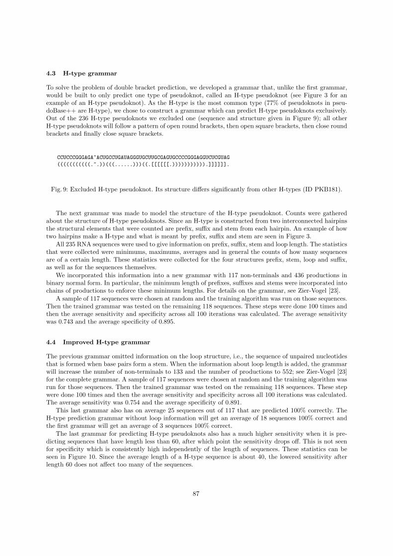
4.3 H-type grammar
To solve the problem of double bracket prediction, we developed a grammar that, unlike the first grammar,would be built to only predict one type of pseudoknot, called an H-type pseudoknot (see Figure 3 for anexample of an H-type pseudoknot). As the H-type is the most common type (77% of pseudoknots in pseu-doBase++ are H-type), we chose to construct a grammar which can predict H-type pseudoknots exclusively.Out of the 236 H-type pseudoknots we excluded one (sequence and structure given in Figure 9); all otherH-type pseudoknots will follow a pattern of open round brackets, then open square brackets, then close roundbrackets and finally close square brackets.
CCUCCCGGGAGA~ACUGCCUGAUAGGGUGCUUGCGAGUGCCCCGGGAGGUCUCGUAG
(((((((((((.~.))(((......)))((.[[[[[[.))))))))))).]]]]]].
Fig. 9: Excluded H-type pseudoknot. Its structure differs significantly from other H-types (ID PKB181).
The next grammar was made to model the structure of the H-type pseudoknot. Counts were gatheredabout the structure of H-type pseudoknots. Since an H-type is constructed from two interconnected hairpinsthe structural elements that were counted are prefix, suffix and stem from each hairpin. An example of howtwo hairpins make a H-type and what is meant by prefix, suffix and stem are seen in Figure 3.
All 235 RNA sequences were used to give information on prefix, suffix, stem and loop length. The statisticsthat were collected were minimums, maximums, averages and in general the counts of how many sequencesare of a certain length. These statistics were collected for the four structures prefix, stem, loop and suffix,as well as for the sequences themselves.
We incorporated this information into a new grammar with 117 non-terminals and 436 productions inbinary normal form. In particular, the minimum length of prefixes, suffixes and stems were incorporated intochains of productions to enforce these minimum lengths. For details on the grammar, see Zier-Vogel [23].
A sample of 117 sequences were chosen at random and the training algorithm was run on those sequences.Then the trained grammar was tested on the remaining 118 sequences. These steps were done 100 times andthen the average sensitivity and specificity across all 100 iterations was calculated. The average sensitivitywas 0.743 and the average specificity of 0.895.
4.4 Improved H-type grammar
The previous grammar omitted information on the loop structure, i.e., the sequence of unpaired nucleotidesthat is formed when base pairs form a stem. When the information about loop length is added, the grammarwill increase the number of non-terminals to 133 and the number of productions to 552; see Zier-Vogel [23]for the complete grammar. A sample of 117 sequences were chosen at random and the training algorithm wasrun for those sequences. Then the trained grammar was tested on the remaining 118 sequences. These stepwere done 100 times and then the average sensitivity and specificity across all 100 iterations was calculated.The average sensitivity was 0.754 and the average specificity of 0.891.
This last grammar also has on average 25 sequences out of 117 that are predicted 100% correctly. TheH-type prediction grammar without loop information will get an average of 18 sequences 100% correct andthe first grammar will get an average of 3 sequences 100% correct.
The last grammar for predicting H-type pseudoknots also has a much higher sensitivity when it is pre-dicting sequences that have length less than 60, after which point the sensitivity drops off. This is not seenfor specificity which is consistently high independently of the length of sequences. These statistics can beseen in Figure 10. Since the average length of a H-type sequence is about 40, the lowered sensitivity afterlength 60 does not affect too many of the sequences.
87

(a) Sensitivity (b) Specificity
Fig. 10: (a) A break down of average sensitivity for 100 tests based on various length sequences. (b) A breakdown of an average specificity for 100 tests based on various length sequences.
5 Discussion
Our prediction algorithm relies on the CYK algorithm, which has a time complexity of O(n3m) and spacecomplexity of O(n2m) where n is the length of a sequence and m is the number of non-terminals in thegrammar. Previous grammar based predictors, for example, the pair stochastic tree adjoining grammardesigned by [13], had more intensive run-times. For instance, the pair stochastic tree adjoining algorithmhas a running time of O(n5).
Even though the model of Matsui et al. [13] has a higher sensitivity, our algorithm performs our predictionsfaster. Also, the model of Matsui et al. [13] does not have the versatility of being able to predict all H-typessequences but can only make predictions based on phylogenetic family.
6 Conclusions and Future Work
In this paper we extended the class of CGs to SCGs. This extension allows SCGs to be used for machinelearning in bioinformatics. We also provided a generalized CYK algorithm for SCGs.
We also designed grammars that were able to predict RNA pseudoknotted secondary structure. We wereunable to build a grammar that was able to predict all types of pseudoknots successfully. However, whenwe focused the predictions to only H-type pseudoknots, the grammars were very successful with an averagesensitivity of over 75% and an average specificity of over 89%. It may be difficult to extend our grammarto other pseudoknot types as there are few training examples. Currently, pseudoBase++ lists just over 70non-H-type pseudoknotted sequences.
As well, it would be interesting to find other kinds of problems that this class of grammars can be appliedto in bioinformatics, including possibly RNA-RNA interaction prediction, which was previously consideredby Kato et al. [10].
References
1. T. Akutsu. Dynamic programming algorithms for RNA secondary structure prediction with pseudoknots. DiscreteApplied Mathematics, 104(1–3):45–62, 2000.
2. P. Bildi and S. Brunak. Bioinformatics: The Machine Learning Approach. The MIT Press, 2001.3. Ian Brierley, Simon Pennell, and Robert J. C. Gilbert. Viral RNA pseudoknots: versatile motifs in gene expression
and replication. Nature Reviews Microbiology, 5:598–610, August 2007.4. M. Brown and C. Wilson. RNA pseudoknot modeling using intersections of stochastic context free grammars
with applications to database search. In Pacific Symposium on Biocomputing, pages 109–125. 1996.
88

5. L. Cai, R. Malmberg, and Y. Wu. Stochastic model of RNA pseudoknotted structures: a grammatical approach.Bioinformatics, 19(1):66–73, 2003.
6. R. Durbin, S. Eddy, A. Krogh, and G. Mitchison. Biological sequence analysis. Cambridge University Press, 1998.7. S. Eddy and R. Durbin. RNA sequence analysis using covariance models. Nucleic Acids Research, 22(11):2079–
2088, 1994.8. Z. Esik and W. Kuich. Boolean fuzzy sets. International Journal of Foundations of Computer Science, 18(6):1197–
1207, 2007.9. X.-Y. Fang, Z.-G. Luo, and Z.-H. Wang. Predicting RNA secondary structure using profile stochastic context-free
grammars and phylogenic analysis. Journal of Computer Science and Technology, 23(4):582–589, 2008.10. Y. Kato, T. Akutsu, and H. Seki. A grammatical approach to RNA–RNA interaction prediction. Pattern
Recognition, 42(4):531–538, 2006.11. Y. Kato, H. Seki, and T. Kasami. RNA pseudoknotted structure prediction using stochastic multiple context-free
grammar. IPSJ Digital Courier, 2:655–664, 2006.12. D. Mathews, S. Schroeder, D. Turner, and M. Zuker. Predicting RNA secondary structure. In R. Gesteland,
T. Cech, and J. Atkins, editors, The RNA World. Cold Spring Harbor Laboratory Press, 2006.13. H. Matsui, K. Sato, and Y. Sakakibara. Pair stochastic tree adjoining grammars for aligning and predicting
pseudoknot RNA structures. Bioinformatics, 21(11):2611–2617, 2005.14. A. Okhotin. Conjunctive grammars. Journal of Automata, Languages and Combinatorics, 6(4):519–535, 2001.15. A. Okhotin. Conjunctive and Boolean grammars: the true general case of the context-free grammars. Preprint
available at http://users.utu.fi/aleokh/papers/boolean_survey.pdf, 2012.16. Sanguthevar Rajasekaran, Sahar Al Seesi, and Reda A. Ammar. Improved algorithms for parsing ESLTAGs:
A grammatical model suitable for RNA pseudoknots. IEEE/ACM Transactions on Computational Biology andBioinformatics, 7(4):619–627, 2010.
17. E. Rivas and S. Eddy. The language of RNA: a formal grammar that includes pseudoknots. Bioinformatics,16(4):334–340, 2000.
18. Y. Sakakibara, M. Brown, R. Underwood, I. Mian, and D. Haussler. Stochastic context-free grammars formodeling RNA. Proceedings of the Twenty-Seventh Annual Hawaii International Conference on System Sciences:Biotechnology Computing, 5:284–293, 1994.
19. Yasubumi Sakakibara. Grammatical inference in bioinformatics. IEEE Transactions on Pattern Analysis andMachine Intelligence, 27(7):1051–1062, 2005.
20. D. Staple and S. Butcher. Pseudoknots: RNA structures with diverse functions. PLoS Biology, 3:e213, 2005.21. M. Taufer, A. Licon, R. Araiza, D. Mireles, F. H. D. van Batenburg, A. Gultyaev, and M.-Y. Leung. Pseu-
dobase++: an extension of pseudobase for easy searching, formatting and visualization of pseudoknots. NucleicAcids Research, 37:D127–D134, 2009.
22. Yasuo Uemura, Aki Hasegawa, Satoshi Kobayashi, and Takashi Yokomori. Tree adjoining grammars for RNAstructure prediction. Theoretical Computer Science, 210:277–303, 1999.
23. R. Zier-Vogel. Predicting RNA secondary structure using a stochastic conjunctive grammar. Master’s thesis,University of Manitoba, http://hdl.handle.net/1993/8453, 2012.
24. M. Zuker and P. Stiegler. Optimal computer folding of large RNA sequences using thermodynamics and auxiliaryinformation. Nucleic Acids Res., 9:133–148, 1981.
89

A Kripke model for subrecursion
Joaquın Dıaz Boils1 and Jose P. Ubeda2
1 Departament de MatematiquesUniversitat Jaume I de Castello
[email protected] Departament de Logica y Filosofia de la Ciencia
Universitat de [email protected]
Abstract. A new point of view of Symmetric Monoidal Comprehen-sions is introduced to give an analogous interpretation about how somesubrecursive function classes can be categorically constructed. It is given,in particular, a general setting to perform subrecursive hierarchies likethe known as Grzegorzcyk Hierarchy. That is done by constructing acategory intended to emulate safe recursion and composition.
Keywords: Symmetric monoidal Comprehension, Grzegorzcyk Hierar-chy, Safe recursion, Applicative structure, Kripke model.
1 Introduction
J. Otto in [10] suggests a close relation between Kripke structures and com-position of functions in the sense of S. J. Bellantoni and J. Cook [1]. He givesa characterization of the first three levels of Grzegorzcyk Hierarchy by usingsymmetric monoidal 2- and 3-Comprehensions.
Based on results of M. Wirz [11] and S. J. Bellantoni and S.J. Niggl [2]and generalizing concepts of J. Otto, we give in [4] a categorical counterpart ofgeneralized safe composition and safe recursion. A new categorical setting wasdefined in order to characterize the subrecursive classes belonging to (the whole)Grzegorzcyk Hierarchy. This was achieved by means of coercion functors overa symmetric monoidal category endowed with certain recursion schemes thatimitate the known as bounded recursion scheme.
We summarize those concepts in Section 2 and remite the reader to [4] for de-tails. In that section a diferent point of view of subrecursion, and of GrzegorzcykHierarchy in particular, is given. By considering Kripke applicative structures weintroduce in Section 3 a general setting for subrecursion which is specialized (asa Kripke model) to the Grzegorzcyk Hierarchy in Section 4. It can be of interestbecause of the fact that Kripke models are more readable for non experts inCategory Theory and because they have been developed more extensively thancategorical comprehensions. In section 5 we show how a cartesian category thatcontains a general instance of safe recursion and safe composition in categorical
90

terms can be defined. It is called in that section a safe semantic category. Sec-tion 6 exposes briefly a summary of the results presented and future researchdirections starting from it.
2 Categorical characterization of Grzegorzcyk hierarchy
Definition 1. We denote by n the (symmetric monoidal) category whose set ofobjects is n = 0, 1, . . . , n− 1 and whose arrows, denoted by mi,j with 0 ≤ i ≤j < n, are those unique mi,j : i −→ j.
Definition 2. Let be for 0 ≤ k < n− 1 functors id : n −→ n, Tk : n −→ n andGk : n −→ n such that for all j ∈ n:
id(j) = j Tk(j) =
j + 1 if j = kj if j 6= k
Gk(j) =
j − 1 if j = k + 1j if j 6= k + 1
We will refer to Tk and Gk as coercion functors.
Definition 3. Let εk : Gk =⇒ id and ηk : id =⇒ Tk (0 ≤ k ≤ n − 2) be suchthat
εk(i) =
mi,i if i 6= k + 1mi−1,i if i = k + 1
ηk(i) =
mi,i if i 6= kmi,i+1 if i = k
for i = 0, ..., n− 1.
We say that, given a symmetric monoidal category (SM category in thesequel3) C = (C,⊗,>, a, l, σ), a tuple (C,
⟨T Ck⟩,⟨GCk⟩,⟨ηCk⟩,⟨εCk⟩) is a model of
(n, 〈Tk〉 , 〈Gk〉 , 〈ηk〉 , 〈εk〉) if T Ck , GCk , ηCk and εCk satisfy the same commutativediagrams than Tk, Gk, ηk and εk (0 ≤ k < n− 1).
Definition 4. A SM n-Comprehension is a tuple (C,⟨T Ck⟩,⟨GCk⟩,⟨ηCk⟩,⟨εCk⟩)
(0 ≤ k < n− 1) where
1. C is a SM category;
2. for every k such that 0 ≤ k < n − 1 the functors T Ck , GCk : C −→ C are SM
functors;
3. for every k such that 0 ≤ k < n−1 the natural transformations ηCk : id =⇒ T Ckand εCk : GCk =⇒ id are SM transformations;
4. (C,⟨T Ck⟩,⟨GCk⟩,⟨ηCk⟩,⟨εCk⟩) is a model of (n, 〈Tk〉 , 〈Gk〉 , 〈ηk〉 , 〈εk〉).
Definition 5. We define doctrines An as those whose objects are SM n-Compre-hensions (C, 〈Tk〉 , 〈Gk〉 , 〈ηk〉 , 〈εk〉) with 0 ≤ k ≤ n− 2
3 Concepts are taken from [6] and [10].
91

– endowed with a diagram (named initial diagram) > 0−→ N0s−→ N0 in C
such thatT0(> 0−→ N0
s−→ N0) = > 1>−→ > 1>−→ >where, if we define recursively for each i = 1, 2, ..., n− 2 the objects Ni by
N1 = G0N0 Ni+1 = GiNi
we have for each i = 0, 1, ..., n− 2 and j = 0, 1, ..., n− 1
TiNj =
> if i = j = 0
Ni−1 if i = j 6= 0
Nj other
GiNj =
Ni+1 if i = j
Nj other
– closed under• flat recursion: for all g : X −→ Y and h : N0⊗X −→ Y where T0X andT0Y are isomorphic to > there exists a unique morphism f : N0⊗X −→Y in C such that the following diagram commutes
>⊗X 0⊗X //
gl((RRRRRRRRRRRRRRR N0 ⊗Xf
N0 ⊗X
huulllllllllllllll
s⊗Xoo
Y
• safe ramified recursion on each level k: for all k = 0, 1, ..., n − 2 andfor all morphisms g : X −→ Y and h : Y −→ Y where Tk+1...T0Y isisomorphic to > there exists a unique f : Nk+1 ⊗ X −→ Y in C suchthat the following diagram commutes
>⊗X 0⊗X //
l
Nk+1 ⊗X s⊗X //
f
Nk+1 ⊗Xf
X g
// Yh
// Y
– for all cartesian object4 in n-Comprehensions (C,⟨T Ck⟩,⟨GCk⟩,⟨ηCk⟩,⟨εCk⟩)
it is also closed under safe dependent recursion in each level k: for all k =0, 1, ..., n− 2 and all morphisms g : X −→ Y and h : (Nk+1⊗X)⊗Y −→ Ywhere Tk...T0Y is isomorphic to > and X and Y are cartesian objects thereexists a unique f : Nk+1 ⊗ X −→ Y in C such that the following diagramcommutes
>⊗X0k+1⊗X //
(0k+1⊗X),gl ))TTTTTTTTTTTTTTT Nk+1 ⊗Xsk+1⊗X //
id,f
Nk+1 ⊗Xf
(Nk+1 ⊗X)⊗ Y
h// Y
4 We call cartesian objects in An the objects in the formn−1⊗i=0
Nαii .
92

Example 1. We consider Set as a SM category (actually a cartesian SM withthe tensor product given by (×, 1)).
– let be the sets Nk = (k, n)/n ∈ N with k = 0, 1, ..., n− 1;– we denote every pair (k, n) by nk;– let be sk(nk) = (n + 1)k for k = 0, ..., n − 2 and nk ∈ Nk the successor
function in Nk;– let Tk be the endofunctor in Set defined by
TkX =
∅ if k = 0 and X = (0, n) with n ∈ N1 if k = 0 and X = N0
(k − 1, n) if k 6= 0 and X = (k, n) with n ∈ NNk−1 if k 6= 0 and X = NkTkY ⊗ TkZ if X = Y ⊗ ZX other
– analogously we can define an endofunctor Gk by
GkX =
(k + 1, n) if X = (k, n) with n ∈ NNk+1 if X = NkGkY ⊗GkZ if X = Y ⊗ ZX other
– let ηk : Gk ⇒ id and εk : id⇒ Tk be natural transformations;
– an initial diagram in Set given by 10−→ N0
s−→ N0;
According to the Definition 5 we have all the equations making
(Set, 〈Tk〉 , 〈Gk〉 , 〈ηk〉 , 〈εk〉)
a SM n-Comprehension.
Proposition 1. The An doctrine is endowed with an initial SM n-Comprehen-sion
(J n, 〈Tk〉 , 〈Gk〉 , 〈ηk〉 , 〈εk〉).We abbreviate it as J n.
Definition 6. Let Γ : J n −→ Set be defined by ΓX = J n(>, X) and Γf =f −.5
Proposition 2. The image of the objects Nk by the functor Γ are sets whoseelements have the form ΓNk = stdkn/n ∈ N where stdk : N −→ ΓNk isdefined by the scheme
stdk0 = 0k
stdk(sn) = sk(stdkn)with k = 0, 1, ..., n− 1
5 This is a special case of the know as global sections functor.
93

Corollary 1. ΓNk = Nk for all k = 0, 1, ..., n− 1.
Definition 7. The binary functions sequence Fj for j ∈ N is recursively definedas:
F0(x, y) = y + 1F1(x, y) = x+ y
F2(x, y) = (x+ 1)(y + 1)
and the scheme
Fn+1(0, y) = Fn(y + 1, y + 1)Fn+1(x+ 1, y) = Fn+1(x, Fn+ 1(x, y))
for n > 1. ([5, p. 28])
Definition 8. We will say that a function class X is closed respect to the oper-ation of bounded recursion if, given three functions g, h, j ∈ X, every functionf satisfying the three following conditions
f(u, 0) = g(u)f(u, x+ 1) = h(u, x, f(u, x))f(u, x) ≤ j(u, x)
belongs to X. ([5, p. 14])
Definition 9. The Grzegorzcyk Hierarchy is the sequence of classes En of nu-meric functions, where En is the smallest class such that:
1. it includes successor, first and second projections and Fn(x, y) as initial func-tions and
2. is closed under the operations of substitution and bounded recursion. ([5, p.29])
We denote by Kn the initial doctrine J n with the difference that we don’t allowany action of a functor Tk over a morphism of it. We also denote by Gn thefunctions set Γf : Nαn−1 −→ Nn−1/α ∈ N, f ∈ Kn.
The following Theorem is the main result of [4, p. 97].
Theorem 1. [Categorical Characterization of Grzegorzcyk Hierarchy]
En = Gn for all n ≥ 3
3 Kripke structures for Grzegorzcyk Hierarchy
The Kripke applicative structures defined by J. Mitchell and E. Moggi [9] gen-eralize the structures defined by S. Kripke in [7] for the intuitionistic logic.
Definition 10. A Kripke applicative structure A is a tuple⟨(W,≤), Aσw, Appσ,τw , iσw,w′
⟩
where
94

– (W,≤) is a partially ordered set of possible worlds;6
– Aσw is a family of sets indexed by types and worlds w ∈W ;– Appσ,τw is a family of application functions Appσ,τw : Aσ→τw × Aσw −→ Aτw
indexed by pairs of types σ and τ and worlds w ∈W ;– iσw,w′ is a family of transition functions iσw,w′ : Aσw −→ Aσw′ indexed by
types σ and worlds w ≤ w′.Under the following conditions:
1. the transition function iσw,w : Aσw −→ Aσw is the identity;2. transition functions compose in the following way iσw′,w′′ iσw,w′ = iσw,w′′ for
each worlds w ≤ w′ ≤ w′′;73. application and transition functions commute in the following sense
iτw,w′(Appσ,τw (f, a)) = Appσ,τw′ ((iσ→τw,w′f), (iσw,w′a))
for each f ∈ Aσ→τw and for each a ∈ Aσw what can be expressed by thefollowing commutative diagram
Aσ→τw′ ×Aσw′Appσ,τ
w′ // Aτw′
Aσ→τw ×AσwAppσ,τw
//
iσ→τw,w′×i
σ
OO
Aτw
iτw,w′
OO
An analogous definition of a Kripke applicative structure could be given bytaking directly a cartesian category where sets Aσw are the (indexed) objectsover a partial ordered set seen itself as a category with a unique arrow betweenevery pair of objects expressing the partial order. In that case, which we don’tdevelope here, App would be (indexed) arrows of the former category. Relatedto the indexing point of view we have the following concepts.
From a Kripke applicative structure A we can define for all type σ a functor
φσ : W −→ Set
given by φσ(w) = Aσw and φσ(lw,w′) = iσw,w′ for each lw,w′ : w −→ w′ such thatw ≤ w′. The conditions making a functor out of φσ for each type σ are satisfiedby conditions 1. and 2. in the definition of Kripke applicative structure.
Definition 11. A global element a of type σ in a Kripke applicative structureA is an assignation w 7→ aw from worlds to elements such that aw ∈ Aσw andwhen w ≤ w′ then iσw,w′aw = aw′ .
6 It can be seen as a category whose objects are the elements of W and its morphismslw,w′ for all w,w′ ∈W such that w ≤ w′.
7 From this we know that there is exactly one transition function from Aσw to Aσw′ forall w ≤ w′.
95

Proposition 3. Every global element a of type σ → τ induces a natural trans-formation from φσ to φτ given by Appσ,τw (aw, ·).Definition 12. We will say that a Kripke applicative structure is extensionalif for every f, g ∈ Aσ→τw such that (iσ→τw,w′f)(a) = (iσ→τw,w′g)(a) with w′ ≥ w anda ∈ Aσw we have f = g.
Definition 13. A Kripke applicative structure is a Kripke model if it is exten-sional and there are no empty types.
4 The Grzegorzcyk Hierarchy by a Kripke model
From the doctrine structure An given in Definition 5 it can be observed thatwhat we are actually constructing is a Kripke (model) structure. It is developedin the following.
The type system we will make use of, and that we will denote as ST becauseof its similarity with known as Simple Type Theory, is specified as follows:
Definition 14. Let be a type system consisting of:
1. natural numbers α as 1-types where(a) if α = 0 we have N0
k = >;(b) if α = 1 we have sets N1
k = Nk;
(c) if α = j + 1 we have sets N j+1k = Nk ⊗N j
k , para 0 < j.2. function types are those in the form α→ β where α and β are 1-types giving
rise to an object Nα→βk subset of (Nβ
k )Nαk .
We are now going to give our main exemple of the functions a Kripke ap-plicative structure like ours can give rise to. If we take W = n as defined above,we can construct a Kripke applicative structure.
⟨n, Nα
k , Appα,βk , iαk,j⟩
which we will denote by RECn.We now give a description of some elements belonging to the (set-theoretic
point of view of) Kn have an interpretation in our Kripke applicative structureRECn:
objects: objects are Nαk with 1-type α and world k where worlds correspond tothe different levels;8
functional objects: objects in the form Nα→βk where α and β are 1-types giving
rise to a subset of (Nβk)Nαk , el conjunto of the morfisms f : Nαk −→ Nβk in Kn;
transition functions: transition functions i1m,j : Nm −→ Nj are the compositefunctors Gj−1...Gm in the SM n-Comprehension (J n, 〈Tk〉 , 〈Gk〉 , 〈ηk〉 , 〈εk〉)for worlds m ≤ j ≤ n − 1. We then also have for α a 1-type, iαm,j as the
functor i1m,j applied to Nαm, remember that functors Gk preserve ⊗;
8 Those defined in [4] as levels of some object N , relating to the work of D. Leivantin [8], to an arbitrary tensor power α; they correspond to the Definition 5.
96

1-type global elements: a 1-type global element α in RECn is an assignationφα from n to RECn such that φα(0) is a vector with α components belongingto Nα0 and for 0 < k < n− 1 we have9
φα(k + 1) = iαk,k+1(φα(k));
functional global elements: a function type global element α → β in RECnis an assignation φα→β from n to RECn such that φα→β(0) is a function in
the set (Nβ0 )Nα0 and for 0 < k < n− 1 we have10
φα→β(k + 1) = iα→βk,k+1(φα→β(k));
general transitions: functors iα→βk,j with k ≤ j in (J n, 〈Tk〉 , 〈Gk〉 , 〈ηk〉 , 〈εk〉)send functions in the form fk : Nαk −→ Nβk to functions in the form11
fj : Nαj −→ Nβj ;
extensionality: RECn is extensional since for all f, g ∈ Nα→βk such that
(iα→βk,j f)(n) = (iα→βk,j g)(n)
with n − 1 ≥ j ≥ k and n ∈ Nαk we have necessarily f = g. This is be-
cause what we get in Nαj are copies of the functions in Nαk making grow theargument levels as it is explained in [4];
recursive operator: every Nα→βk+1 with α and β 1-types contains, for every X =
Nαk+1, Y = Nβk+1, g ∈ Nα→βk and h ∈ N(α+β+1)→β
k , a unique f ∈ N1+α→βk+1
such that the following diagram commutes
>⊗X0k+1⊗X //
(0k+1⊗X),g′l ))TTTTTTTTTTTTTTT Nk+1 ⊗Xsk+1⊗X //
id,f
Nk+1 ⊗Xf
(Nk+1 ⊗X)⊗ Y
h′// Y
where g′ = iα→βk,k+1(g) and h′ = i(α+β+1)→βk,k+1 (h).
It is important to note here that the chosen of the type theory from whichwe build up the applicative structure is crucial for the kind of functions we get.For exemple, consider that the above recursive diagram for RECn could not bedefined from the types available in ST .
We see that RECn contains all functions belonging to E0, . . . , En−1 in theGrzegorzcyk Hierarchy and moreover
⋃n∈NRECn will then contain all primitive
recursive functions.9 In our case, and considering the initial SM n-Comprehension, each vector in Nα
0
gives rise to a global element.10 Functions belonging to the first Grzegorzcyk Hierarchy class E0 are function type
global elements and they also live in all successive En for n > 0.11 fj is obtained by appliying the functor i1k,j to the function fk.
97

Proposition 4. RECn is a Kripke model for every n ∈ N.
Definition 15. Let φα : n −→ Set be the functor given by φα(k) = Nαk andφα(mk,j) = iαk,j for every mk,j : k −→ j such that k, j ∈ n with k ≤ j.
5 Safe semantic categories
Instead of J. Mitchell and E. Moggi [9] given two types α and β such that α 6= β
we can ensure that the sets in RECn in the form Nαk and Nβ
k with k ∈ n belong-ing to the initial SM n-Comprehension J n are different (although isomorphic).In this way the cartesian closed category generated by the Kripke applicativestructure RECn, that we will denote by CRECn in the following definition, canbe constructed from its presheaves and not uniquely from its types (see [9, page15]).
Definition 16. Let CRECn be the category whose objects are functors φα in Setn
from Definition 15 for each α ∈ N and whose morphisms are natural transfor-mations between those functors.
In this way we are considering a subcategory of Setn where the objects inCRECn generate all sets in RECn. Natural transformations in the form φα −→ φβare generated from every arrow mk,j : k −→ j in n by commutative squares
φα(k) //
φα(mk,j)
φβ(k)
φβ(mk,j)
φα(j) // φβ(j)
(1)
As pointed out in [9], CRECn is cartesian if RECn has products and a terminalobject and for every natural number α there exists a unique functor ϕα in CRECn .
Particularly, and looking beyond J n, in CRECn it is formalized a way toperform safe recursion and safe composition: its objects are copies of powers ofN, it can be endowed with a certain safe recursive operator as the one given inSection 4 and it is endowed with coercion functors ϕα(mk,j).
From Proposition 3 we observe that every global element f of type α → βinduces a natural transformation in the form
Appα,β(f, ·) : φα −→ φβ
giving Appα,βk (f,Nαk ) for a set Nα
k in RECn where we supose k to be the domainand codomain world of f . That is, by fixing the first variable in App we areproducing assignations in the form Nα
k −→ Nβk for every world k in n and f
having functional type α→ β in the world k. Natural components of Appα,β(f, ·)are then arrows in Set in the form
Appα,βk (f,Nαk ) : φα(k) −→ φβ(k)
98

and therefore arrows Nαk −→ Nβk .
The naturality condition for Appα,βk (f, ·) expresses safe composition. That is
due to the fact that in it an expression of every morphism f ∈ Nα→βj in RECn
is obtained in terms of other morphisms where the variables belong to the worldj. An output belonging to a world j, in general, does not depend on inputsbelonging to worlds lower than j.
That is, elements and concepts in CRECn gather the semantics of safety andtherefore it can be viewed as a safe semantic category for a certain Kripkeapplicative structures.
6 Conclusion and future work
The content of this talk is the initial point of a further study to get a fulldescription of subrecursive function classes from Kripke models. For that purposeone could get rid of comprehension structures as defined here to work just witha Kripke applicative structure endowed with certain recursion schemes. It wouldmake extensive use of the categorical concept of presheaf. This line is currentlybeing developed.
References
1. Bellantoni, S. J., Cook, S.: New Recursion-Theoretic Characterization of the Poly-time Functions. Comput. Complexity 2, 97–110 (1992)
2. Bellantoni, S. J., Niggl, K.: Ranking Primitive Recursions: the Low GrzegorczykClasses Revisited. SIAM J. Comput. 29(2), 401–415 (1999)
3. Clote, P.: Computation models and function algebras. In: Griffor, E.R. (ed) Hand-book of Computability Theory, pp. 589-681. Elsevier Science B.V. (1999).
4. Dıaz Boils, J.: Comprensiones Categoriales y Subrecursion. PhD Thesis. Universitatde Valencia (2012) Available at: http://roderic.uv.es/handle/10550/24423
5. Grzegorczyk, A.: Some classes of recursive functions. Rozprawy matematyczne 4,1–45, (1953)
6. Kelly, G. M.: Basic Concepts of Enriched Category Theory. Reprints in Theory andApplications of Categories 10, (2005)
7. Kripke, S.: Semantical Analysis of Intuitionistic Logic I. In: Dummett, M., J. N.Crossley, J. N. (eds) Formal Systems and Recursive Functions, pp. 92–129. NorthHolland (1965)
8. Leivant, D.: Ramified recurrence and computational complexity I: Word algebrasand polytime. In: Clote, P., Remmel, J. (eds.) Feasible Mathematics II, pp. 320–343.Birkhause (1994)
9. Mitchell, J., Moggi, E.: Kripke-style models for typed lambda calculus. Journal ofPure and Applied Algebra 51, 99–124 (1991) Available at: www.disi.unige.it/
person/MoggiE/ftp/kripke.pdf
10. Otto, J.: Complexity Doctrines. Ph.D. thesis, McGill University (1995)11. Wirz, M.: Characterizing the Grzegorczyk hierarchy by safe recursion. CiteSeer,
(1999) http://citeseerx.ist.psu.edu/viewdoc/summary?doi=10.1.1.42.3374.
99

How to reduce backtracking in propositionalIntuitionistic logic
Guido Fiorino
Dipartimento di Informatica Sistemistica e Comunicazione, Universita degli Studi diMilano-Bicocca, P.zza dell’Ateneo Nuovo 1, 20126 Milano, Italy
Abstract. We discuss a technique to reduce search space in proposi-tional Intuitionistic logic. Our technique is a syntactical criterion basedon the sign property and can be used by any kind of calculus.
1 Introduction
In this paper we continue our investigations to speed-up proof search in propo-sitional Intuitionistic logic (Int). In [3] we have introduced a calculus that ad-vances the well-known calculus of [8], in [5] we have identified conditions allowingone to replace propositional variables with logical constants and an implementa-tion of these achievements is the prover fCube [4]. In the cited papers the focusis on the rules or on the logical apparatus as a whole and the strategy using thecalculus is not considered. In this note we introduce a criterion applicable to anystrategy to reduce the non-determinism in Int proof search. To sake of concrete-ness, we present our results applied to a specific tableau calculus. However, itwill be clear that our results can be applied to any tableau or sequent calculus.
Every step of a deduction has multiple choices and if the proof search fails,then every step is a point where to backtrack because the order of application ofthe rules is relevant, that is, not permutable. However, there is a special kind ofrules that does not require to backtrack, because if a rule of this kind is used anda proof is not found, then no proof exists. This kind of rules is called invertible:the lack of a proof for the conclusion of an invertible rule implies the lack of aproof for the premise. The order of application of invertible rules is irrelevant:different permutations of their application always brings to the same result. Onthe other hand, the non-invertible rules require to backtrack: the lack of a prooffor the conclusion of a non-invertible rule does not imply the lack of a proof forthe premise. The application of non-invertible rules is not permutable, becausedifferent permutations of their applications produce different results. Thus, if ina step of a deduction a non-invertible rule R is applied and subsequenty to thisstep no proof is not found, then a different application of R or the application ofa different rule could bring to find a proof. Note that such application is uselessif we already know that it does not bring to find a proof.
Thus, it is useful to find strategies to reduce as much as possible the appli-cation of non-invertible rules, because this shrinks the search space for a proof.The aim of this paper is to present a criterion to get this goal. This work can be
100

∆,T(A ∧ B)
∆,TA,TBT∧
∆,T(A ∨ B)
∆,TA | ∆,TBT∨
∆,TA,T(A → B)
∆,TA,TBMP
∆,T((A ∧ B) → C)
∆,T(A → (B → C))T→∧
∆,T((A ∨ B) → C)
∆,T(A → C),T(B → C)T→∨
∆,F(A1 ∨ A2)
∆,FAi
F∨i, i ∈ 1, 2
∆,F(A ∧ B)
∆,FA | ∆,FBF∧
∆,F(A → B)
∆,TA,FBF→
∆,T((A → B) → C)
∆T,TA,FB,T(B → C) |∆,TCT→→ where ∆T = TA | TA ∈ ∆
Fig. 1. The calculus
seen as an extension of [2] where the syntax of sequent calculus LJQ gives rise toa strategy allowing to avoid some backtracking steps. The criterion we presentis strictly related to our previous investigations in [5]. For this reason, after thepreliminaries, we first describe a logical rule that generalizes the permanencerules of [5]. The application of our rule is subjected to a syntactical conditionwhich subsumes the syntactical condition for the permanence rules of [5]. Weuse this syntactical condition to design a decision procedure that under somesyntactical conditions avoids the application of non-invertible rules. The mainwork is to prove that the decision procedure is complete, a result that we showby exploiting the model theoretic characterization of Int by means of Kripkemodels.
2 Preliminaries
We consider the propositional language L based on a denumerable set of propo-sitional variables PV, the logical connectives ∧, ∨,→ and the logical constants >and ⊥. We refer to [1,6,7] for details about Int and tableau systems. For sake ofconcreteness we consider the terminating calculus in Figure 1 whose rules handlesigned formulas, namely formulas of L prefixed with one of the well-known signsT or F. The satisfiability of a signed formula H in a world α of a Kripke modelK is defined as follows: α realizes H in K (K,αH) iff: (i) H ≡ TA and α A;(ii) H ≡ FA and α 1 A. A model K realizes H (K H) iff K,αH for someα ∈ P ; a formula H is realizable iff K H for some Kripke model K .When possible, in the following sections we will omit notation and we write:α H and α ∆ in place of K ,α H and K ,α ∆ when it is clear from thecontext to which model the realizability relation refers to.
The tableau calculus of Figure 1 is adapted from the calculus presented in [9].Our aim is to consider a simple tableau calculus to decide Int, whose deductionsare always finite. Thus, differently from [9], calculus in Figure 1 does not handlenegation and only employs the signs T and F. Calculus of Figure 1 has alsosimilarities with Fitting’s tableau calculus [6]. In the rules of the calculus wedistinguish the premise, the set of formulas above the line and the consequence,the set(s) of formulas below the line that we call conclusion(s), separated by avertical line when the consequence of the rule contains two conclusions. In thepremise, the main formula of the premise is the formula whose connectives are inevidence, the other formulas are the minor formulas of the premise. The formulas
101

in evidence in a conclusion are the main formulas of the conclusion. We say thata rule applies to a set of formulas Γ , if the premise of the rule can be instantiatedwith Γ . We implicitly always consider duplication-free instantiations, that is afterthe instantiation of the premise of a rule, the main formula premise does notoccur in ∆ (that is, it does not occur as minor formula premise). Given a non-atomic signed formula H, we denote with Rule(H) the name of the rule whosemain formula premise can be instantiated with H. A set Γ of signed formulas isinconsistent if TA,FA ∈ Γ or T⊥ ∈ Γ and Γ is consistent in the other cases.A tableau for a formula A is a tree obtained from the root FA by subsequentlyinstantiating the premise of a rule with consistent leaves. If all the leaves of atableau are inconsistent, then we say that the tableau is closed, the tableau is aproof for A and A is provable.The rules in Figure 1 are sound: the realizability of the premise implies thatthere exists a conclusion which is realizable. It is easy to prove that calculusin Figure 1 is also complete for Int: for every formula A, A is provable iff FAis not realizable. To decide the provability of A it is sufficient to search for aclosed tableau. An obvious algorithm tries to build a proof for A by applying therules in all possible ways. This simple method can be improved by noticing thatsome rules are invertible: the realizability of one of the sets in the conclusionimplies the realizability of the premise. Thus backtracking is not required whenan invertible rule is applied. This is a well-known strategy, also employed in [6,9].We remark that such a strategy based on the calculi in Figure 1 and in [9] isterminating. In the following sections we aim to show that further restrictionsto the search space of proofs are possible. Thus it should be possible to reducethe backtrack and preserve the completeness.Our first result is a generalization of the permanence rules introduced in [5]to reduce the search space. When a propositional variable p fulfills a syntacticconstraint, the permanence rules allow to deduce a set where all the occurrencesof p are replaced with a logical constant. The syntactic constraint is definedin terms of positive and negative occurrence of a propositional variable p in asigned formula H by the relations p+H (p positively occurs in H) and p−H(p negatively occurs in H). Hereafter we use S to denote either T or F. Thedefinition of plH, with l ∈ +,−, is by induction on the structure of H:(i) p−Fp and p+ Tp; (ii) pl S> and pl S⊥; (iii) pl Sq, where q is anypropositional variable such that q 6= p; (iv) pl S(AB) iff pl SA and pl SB,where ∈ ∧,∨; (v) pl F(A→ B) iff plTA and pl FB; (v) plT(A→ B)iff pl FA and plTB. Given a set ∆ of signed formulas, pl∆ iff for everyH ∈ ∆, plH. In paper [5] it is proved that permanence rules given in thefollowing are invertible:
∆
∆[>/p]T-perm, provided p+∆
∆
∆[⊥/p]T→ ⊥-perm, provided p−∆,
where ∆[A/B] is the result of replacing in ∆ every occurrence of B with A.Intuitively, these rules state that, given a set ∆, if the syntactical constraintp+∆ (resp. p−∆) is fulfilled, then it is correct to replace every occurrenceof p in ∆ with the logical constant > (resp. ⊥).
102

3 An extension of the permanence rules
Now we aim to study a weaker condition for the correct application of rulesT-perm and T→ ⊥-perm. By exploiting such a weaker condition, in next sec-tion we introduce a decision procedure allowing to reduce the search space inproof search for Int. The procedure we describe does not need to employ thepermanence rules as further rules of the logical apparatus. This means that theresults we show are not tied neither to the calculus given in Figure 1 nor to theproof system: a decision procedure based on new tableau calculus or a sequentcalculus can use our results to reduce the search space for a proof.
As first step, let us go back over the side conditions on the applicability ofthe permanence rules. To this aim we introduce a new notion of replacement. LetH be a signed formula and let p a propositional variable. We define replacementin a formula H of all positive occurrences of a propositional variable p with >,the formula denoted with HJ>/pK, obtained from H as follows:
– if H = Tp, then HJ>/pK = T>;– if H = Tq, with q ∈ PV \ p, then HJ>/pK = H;– if H = Fq, then HJ>/pK = H, q ∈ PV;– if H = S(A1 A2), then HJ>/pK = S(A′1 A′2), with SA′i = SAiJ>/pK, fori = 1, 2, S ∈ T,F and ∈ ∧,∨;
– if H = F(A → B), then HJ>/pK = F(A′ → B′), where TA′ = TAJ>/pKand FB′ = FBJ>/pK;
– if H = T(A → B), then HJ>/pK = T(A′ → B′), where FA′ = FAJ>/pKand TB′ = TBJ>/pK.
The following are examples of replacement of q and p respectively:F(p→ (q ∨ q → ⊥))J>/qK = F(p→ (q ∨ > → ⊥));F((p ∨ p→ ⊥)→ q)J>/pK = F((> ∨ p→ ⊥)→ q).
Analogously, we define replacement in a formula H of all negative occurrencesof a propositional variable p with ⊥, the formula denoted with HJ⊥/pK obtainedfrom H as follows:
– if H = Tq, then HJ⊥/pK = H, if q ∈ PV;– if H = Fp, then HJ⊥/pK = F⊥;– if H = Fq, with q ∈ PV \ p, then HJ⊥/pK = H;– if H = S(A1 A2), then HJ⊥/pK = S(A′1 A′2), with SA′i = SAiJ⊥/pK,i ∈ 1, 2, S ∈ T,F and ∈ ∧,∨;
– if H = F(A → B), then HJ⊥/pK = F(A′ → B′), where TA′ = TAJ⊥/pKand FB′ = FBJ⊥/pK;
– if H = T(A → B), then HJ⊥/pK = T(A′ → B′), where FA′ = FAJ⊥/pKand TB′ = TBJ⊥/pK.
The result of HJ>/pK (resp. HJ⊥/pK) is a formula having the same sign of Hand containing zero or more occurrences of the logical constant >(resp. ⊥).Hereafter we use JK-replacement to refer to both kind of replacements definedabove. We extend JK-replacement to sets of signed formulas in the obvious way. If
103

p+∆ (resp. p−∆), then ∆J>/pK (resp. ∆J⊥/pK) coincides with ∆[>/p] (resp.∆[⊥/p]). Given a signed formula H and a set of signed formulas ∆, we writeHJK (resp. ∆JK) to refer both formula HJ>/pK and HJ⊥/pK (resp. set ∆J>/pKand ∆J⊥/pK). Let A be a formula, eval (A) denotes the formula obtained byapplying to A the usual boolean reductions based on the meaning of the logicalconstants. Given a signed formula SA, where S ∈ T,F, the evaluation of asigned formula SA, denoted as eval(SA), is the signed formula Seval(A). Thefollowing is the evaluation of the formulas obtained from the previous example:eval(F(p→ (q ∨ q → ⊥))J>/qK) = eval(F(p→ (q ∨ > → ⊥))) = F(p→ q);eval(F((p ∨ p→ ⊥)→ q)J>/pK) = eval(F((> ∨ p→ ⊥)→ q)) = Fq.The invertibility of the boolean simplification rules implies that HJ∇/pK is re-alizable iff eval(HJ∇/pK) is realizable, with ∇ ∈ >,⊥. The following Propo-sitions 1 and 2 aim to give the whole picture of the relationship between therealizability of H and eval(HJ∇/pK). We start with a technical lemma:
Lemma 1. Let H be a formula such that eval(H) = H, H 6= > and H 6= ⊥ andlet p be a propositional variable. The following holds: 1. eval(THJ∇/pK) 6= T⊥,with ∇ ∈ >,⊥; 2. eval(FHJ∇/pK) 6= F>, with ∇ ∈ >,⊥.The following proposition introduces the condition under which JK-replacementpreserves the realizability. Thus the proposition is a result about the correctnessof JK-replacement:
Proposition 1. Let K = 〈P,≤,ρ, 〉 be a Kripke model, let α ∈ P , let H be asigned formula and let p be a propositional variable: 1. if αH and p does notoccur in eval(HJ>/pK), then αeval(HJ>/pK); 2. if αH and p does not occurin eval(HJ⊥/pK), then α eval(HJ⊥/pK).Let K = 〈P,≤, ρ, 〉 be a Kripke model and p a propositional variable. Follow-ing [5], we define the models K+
p and K−p as follows: K+p = 〈P,≤, ρ, ′〉, where
′ = ∪(α, p) | α ∈ P; K−p = 〈P,≤, ρ, ′〉, where ′ = \(α, p) | α ∈ P.Note that, for every α ∈ P , K+
p , α Tp and K−p , α T(p → ⊥). In followingwe prove that JK-replacement preserves the completeness:
Proposition 2. Let K = 〈P,≤,ρ, 〉 be a Kripke model, α ∈ P , H a signedformula and p be a propositional variable. 1. Let us assume that p does not occurin eval(HJ>/pK). If K,α eval(HJ>/pK), then K+
p , α H; 2. Let us assume
that p does not occur in eval(HJ⊥/pK). If K,αeval(HJ⊥/pK), then K−p , αH.
Now, let us consider the following independence rules:∆
∆[>/p]+-indep, provided p 6∈ PV(eval(∆J>/pK))
∆
∆[⊥/p]−-indep, provided p 6∈ PV(eval(∆J⊥/pK))
By Propositions 1 and 2 we get:
Theorem 1. The rules +-indep and −-indep are invertible.
The notion of JK-replacement can be extended to the replacement of two or morepropositional variables. Let p = p1, . . . , pn and q = q1, . . . , qm be two setsof propositional variables. We define
104

HJ>/p1, . . . ,>/pn,⊥/q1, . . . ,⊥/qmK = HJ>/p,⊥/qK, where p ∩ q = ∅,as follows:
– if H = Tv, then HJ>/p,⊥/qK =
T> if v ∈ pH otherwise
– if H = Fv, then HJ>/p,⊥/qK =
F⊥ if v ∈ qH otherwise
– if H = S(A1 A2), then HJ>/p,⊥/qK = S(A′1 A′2),with SA′i = SAiJ>/p,⊥/qK, for i = 1, 2, S ∈ T,F and ∈ ∧,∨;
– if H = F(A → B), then HJ>/p,⊥/qK = F(A′ → B′), where TA′ =TAJ>/p,⊥/qK and FB′ = FBJ>/p,⊥/qK;
– if H = T(A → B), then HJ>/p,⊥/qK = T(A′ → B′), where FA′ =FAJ>/p,⊥/qK and TB′ = TBJ>/p,⊥/qK.
In a similar way we can define the meaning of H[>/p,⊥/q]. The extension ofthese notions to sets of formulas is obvious. The rule
∆
∆[>/p,⊥/q]±-indep, provided (p ∪ q) ∩ PV(eval(∆J>/p,⊥/qK)) = ∅ and p ∩ q = ∅
generalizes +-indep and −-indep and is invertible. When (p∪q)∩PV(eval(∆J>/p,⊥/qK)) = ∅ holds we say that the set of variables p ∪ q is independent in ∆. Weremark that the intuitively obvious request p ∩ q = ∅ is necessary to prove theinvertibility of ±-indep, the analogous of Proposition 2. As a matter of fact, ifv ∈ p ∩ q we should build a Kripke model behaving as K+
v and K−v , which isobviously impossible.
Rule ±-indep is a consequence of the definition of JK-replacement and itrepresents a generalization of the permanence rules: under the syntactical condi-tions stated for rule ±-indep, it is possible to replace in a set ∆ the occurrencesof a propositional variable p with a logical constant and such a replacement iscorrect also if neither p+∆ nor p−∆ holds. Since variables are replaced byconstants, rule ±-indep is a mechanism to reduce the search space. Rule ±-indepcan be inserted in a procedure for deciding Int and since permanence rules aresubsumed by ±-indep, they can be removed from the deductive system withoutany loss. To apply ±-indep one has to find an independent set of propositionalvariables fulfilling the side condition for ±-indep. This could be a computation-ally expansive task. We are not interested to use the rule in this way. To boundthe backtracking in Int proof search, the decision procedure we provide checks ifa given set of propositional variables is independent in a set. When the conditionis fulfilled, then rule ±-indep is applicable, but the important point is that inthis case some backtracking steps are avoidable. Summarizing, the independenceof a set of propositional variables in a set of formulas is the key point we use toavoid the backtracking.
4 Reducing backtracking in Int
Now we want to exploit JK-replacement and Propositions 1 and 2 to avoid uselessapplications of non-invertible rules. Since we are going to avoid some rule appli-
105

cations, the question is to prove the decision procedure we provide is complete.To this aim we need to prove the following theorem:
Theorem 2. Let ∆ be a set of T-signed formulas and let K = 〈P,≤,ρ, 〉 be amodel such that ρ∆ and ρ p iff Tp ∈ ∆. Let
Γ = ∆ ∪ Tp1, . . . ,Tpn,Fq1, . . . ,Fqm,T(h1 → H1), . . . ,T(hl → Hl)be a consistent set with p ∩ h = ∅, where p = p1, . . . , pn and h = h1, . . . , hl.If (p ∪ h) ∩ PV(eval(∆J>/p,⊥/hK)) = ∅ holds, then: 1. Γ is realizable by theKripke model M = 〈P,≤, ρ,
M〉 such that
M= ( ∪(P × p)) \ (P × h); 2.
if K, ρ F(A → B) and (p ∪ h) ∩ PV(eval(F(A → B)J>/p,⊥/hK)) = ∅, thenM,ρ F(A→ B).
Roughly speaking, the idea to avoid backtracking as applied in followingFunction Bb, can be explained as follows: let S and S′ be two sets of formulasand M = 〈P,≤,ρ, 〉 a Kripke model such that M,ρ S. We are investigatingunder which syntactical conditions of S and S′ we can change the forcing in M toget a model M ′ = 〈P,≤, ρ, ′〉 such that M ′, ρS′. More precisely, we are askingunder which syntactical conditions the realizability of S implies the realizabilityof S′. This is of interest because, if an attempt to find a proof starting from Sfails, then another attempt starting from another set has possibly to be done. Thefailed attempts witnesses that some sets are realizable by a Kripke model. Thuswe wonder if the failed attempt implies that some other attempts we are goingto try, for example starting from S′, will fail. If we found a general criterion,computationally not expensive, to check if this case, then we can reduce thesearch space and speed-up the procedure: such a criterion is the side conditionstated for rule ±-indep. Function Bb works by locking sets of T-signed formulas.Locked formulas are not at disposal of the backtracking steps in the sense thatFunction Bb does not use locked formulas as main formulas. The idea behindthe locking is to mark a set a formulas having a model. This avoids the uselessbacktracking generated by taking the marked formulas as main formula premiseof the non-invertible rule T →→. To decide a formula A, the call Bb(FA, )is performed, where emphasizes that the second parameter is irrelevant. Rulesare applied according to a priority which is standard: T→→ and F∨i are rulesof the lowest priority because if a proof is not found, they require to backtrack.Function Bb returns a proof or a structure that in completeness theorem isproved to be a Kripke model K = 〈P,≤,ρ, 〉 such that ρ∆. In the following,we call α-rules T∧, T→ ∧, T→ ∨, F→ and β-rules T∨, F∧.
Function Bb(∆,M)1. If ∆ is an inconsistent set, then return the proof ∆;2. If the premise of MP can be instantiated with ∆, where TA and T(A→ B) can belocked or unlocked, then let ∆1 be the conclusion and let π = Bb(∆1,M), where TB
is unlocked in ∆1. If π is a proof, then return the proof∆π
MP, otherwise return π.
3. If the premise of an α-rule can be instantiated with ∆, then let H be the mainformula premise, ∆1 the conclusion and π = Bb(∆1,M). If π is a proof, then return∆π
Rule(H), otherwise return π.
4. If the premise of a β-rule can be instantiated with ∆, then let H be the main premise,∆1 and ∆2 the conclusions and, for i = 1, 2 let πi = Bb(∆i,M). If πi is a structure,
106

with i ∈ 1, 2, then return πi, otherwise return the proof∆
π1|π2
Rule(H).
5. (i) (only backtracking on F∨-formula is required). If ∆T is not empty and all theformulas in ∆T are locked and F(A1 ∨ A2) ∈ ∆, then let ∆i = ∆T ∪ FAi andπi = Bb(∆i,M), for i = 1, 2. If πi is a proof, with i ∈ 1, 2, then return the proof∆πi
F∨i; otherwise, let M = 〈PM ,≤M ,ρM , M 〉 and πi = 〈Pi,≤i, ρi, i〉, for i = 1, 2.
Return the structure K = 〈P,≤,ρ, 〉 defined as follows:P = PM ∪ P1 ∪ P2; ≤ = ≤M ∪ ≤1 ∪ ≤2 ∪(ρ, α)|α ∈ P1 ∪ P2;ρ = ρM ; = M ∪ 1 ∪ 2.
(ii) (Full standard backtracking is required) If ∆T contains an unlocked formula of thekind T((A → B) → C) or, all formulas in ∆T are unlocked and F(A ∨ B) ∈ ∆, thenreturn BackT(∆,M).
(iii) If ∆T contains both locked and unlocked formulas (note that the unlocked formulasare atomic or of the kind T(p→ B)), then let Φ = F(A→ B)|T((A→ B)→ C) ∈ ∆,let ∆U = TA ∈ ∆|TA is unlocked , p = p|Tp ∈ ∆U, q = q|T(q → H) ∈ ∆Uand let K = 〈P,≤,ρ, 〉 be the structure defined as follows:
P = PM ; ρ = ρM ; ≤ = ≤M ; = ( M \(P × q)) ∪ (P × p).(A) If F(A1 ∨A2) 6∈ ∆ and (p ∪ q) 6∈ PV(eval(∆J>/p,⊥/qK)), then return K .
(B) If F(A1 ∨ A2) ∈ ∆ and (p ∪ q) 6∈ PV(eval((∆ ∪ Φ)J>/p,⊥/qK)), then for i = 1, 2,let πi = Bb(∆T∪FAi,K ), where in the recursive call all formulas in ∆T are locked.
If there exists i ∈ 1, 2 such that πi is a proof, then return the proof∆πi
F∨i, else let
πi = 〈Pi,≤i, ρi, i〉; return the structure 〈P ′,≤′, ρ, ′〉 defined as follows:P ′ = P ∪ P1 ∪ P2; ≤′ = ≤ ∪ ≤1 ∪ ≤2 ∪(ρ, α)|α ∈ Pi; ′ = ∪ 1 ∪ 2.
(C) Unlock the formulas in ∆ and return Bb(∆, ).
6. (if we are here F(A ∨B) 6∈ ∆). If all the formulas in ∆T are locked, then (i) returnM , else (ii) return 〈 ρ , (ρ, ρ) , ρ, (ρ, p) |Tp ∈ ∆ 〉.End Function Bb.
Function BackT (∆,M)Let T((Ai → Bi)→ Ci)1≤i≤n = T((A→ B)→ C) ∈ ∆;for i = 1, . . . , n
- let φi = Bb((∆ \ T((Ai → Bi)→ Ci)) ∪ TCi,M), where in the recursive callTCi is not locked and the locking of the other formulas is left unchanged;
- if φi is a structure, then return φi.
Unlock all the formulas in ∆;for i = 1, . . . , n
- let πi = Bb((∆T \ T((Ai → Bi)→ Ci)) ∪ TAi,FBi,T(Bi → Ci), );
- if πi is a proof, then return the proof∆
πi|φi
T→→.
Given the structures πi = 〈Pi,≤i, ρi, i〉, with i = 1, . . . , n, define K = 〈P,≤,ρ, 〉 asfollows:P = ρ ∪n
i=1 Pi; ≤ = ∪ni=1 ≤i ∪(ρ, α)|α ∈ P; = ∪n
i=1 i ∪(ρ, p)|Tp ∈ ∆.If F(A1 ∨A2) 6∈ ∆, then return K .
For i = 1, 2- let πn+i = Bb(∆T ∪ FAi,K ), where in the recursive call all the formulas in ∆T
are locked; if πn+i is a proof, then return the proof∆πn+i
F∨i.
107

Return the structure 〈P,≤,ρ, 〉 defined as follows:
P = ρ ∪n+2i=1 Pi; ≤ = ∪n
i=1 ≤i ∪(ρ, α)|α ∈ P; = ∪n+2i=1 i ∪(ρ, p)|Tp ∈ ∆.
End Function BackT.
Function Bb locks the T-formulas after the application of rule F∨i. When thisstage is reached, the realizability of ∆T has been proved by backtracking stepsinvolving the non-invertible conclusion of the rule T →→ and M is the modelrealizing ∆T. The formulas in ∆T will be unlocked when a new T→→-formulais introduced. If a set Γ only containing locked formulas, signed atomic formulasand T(p → H)-formulas, with Tp 6∈ Γ , is gotten, then, by Theorem 2, wecan decide if the realizability of ∆T implies the realizability of Γ . This check isperformed in Step 5(iii)(A). By construction ∆T ⊆ Γ and ∆T coincides with theformulas of Γ that are locked. Function Bb contains a call to Function BackT.Function BackT implements the backtracking mechanism necessary to handleformulas of the kind T((A → B) → C) and F(A ∨ B). This is a standardphase, necessary to guarantee the completeness of the decision procedure. If afterall possible instantiations of the premise of T →→ with ∆ no proof is found,then the structure K is a Kripke model whose root realizes ∆T ∪ F(A →B)|T((A → B) → C) ∈ ∆. At this point, Bb instantiates, if possible, thepremise of F∨1 and F∨2 with ∆. In the subsequent applications the formulasin ∆T are locked, thus T →→-formulas are not used as main formulas. Thisis also the strategy employed by sequent calculus LJQ [2]. The strategy of Bbdiverges from LJQ by the fact that after an application of F →, LJQ unlocksthe formulas, whereas Bb keeps them locked until the only applicable rules areT →→ or F∨. This corresponds to reach Step 5(ii) or 5(iii). If a new T →→formula appears, then Step 5(ii) is performed and BackT is called. In BackT,when the invertible conclusion of rule T→→ is handled, the locking of the minorpremises is left unchanged. When the non-invertible conclusion of T→→ is usedthe locked formulas of ∆ become unlocked, thus Bb behaves as LJQ. If Step 5(iii)is reached, then it means that subsequently to the locking of the formulas, newT-formulas have been added, but they are atomic or of the kind T(p→ A) only.In Steps 5(iii)(A) and 5(iii)(B) function Bb attempts to avoid backtracking steps.Bb performs a purely syntactic check involving JK-replacement. In practice, Bbchecks if the side condition on the applicability of rule ±-indep is fulfilled. Ithas to be noted that the check in Step 5(iii)(A) is different from the check inStep 5(iii)(B). To prove the completeness for the case of Step 5(iii)(B) we neededto know that the model K obtained from M fulfills the property that for everyT((A → B) → C) ∈ ∆, the root of K realizes F(A → B). Since by hypothesisthe given model M fulfills such a property, the check in Step 5(iii)(B) aims toprove that for every T((A → B) → C) ∈ ∆, the realizability F(A → B) isindependent of the forcing of the propositional variables p1, . . . , pn, q1, . . . , qm.Finally we notice that the check in Step 5(iii)(A) and Step 5(iii)(B) is only basedon the locking and the formulas in the set ∆ at hand.
Let ∆ be a set of formulas. In the next theorem we show that (1) if ∆ doesnot contain locked formulas and Bb(∆, ) returns a structure K , then K is aKripke model such K ∆ and Bb does not require any further information;
108

(2) if ∆ contains some locked formula, M is a Kripke model that realizes ∆T
and Bb(∆,M) returns a structure K , then K ∆ and K is possibly built onthe Kripke model M :
Theorem 3 (Completeness). Let ∆ be a set of formulas. 1. If ∆T does notcontain locked formulas and Bb(∆,M) returns a structure K , then K∆ and Kis defined independently of M ; 2. if ∆T contains a subset Γ of locked formulasand M = 〈PM ,≤M ,ρM , M 〉 is a Kripke model such that M Γ , for everyT((A→ B)→ C) ∈ Γ , there exists α ∈ PM such that ρM 6= α and αTA,FBand ρM p iff Tp ∈ Γ , then Bb(∆,M) returns a structure K such that K ∆.
5 Conclusions and Future Works
We have presented a new optimization rule called ±-indep that generalizes thepermanence rules given in [5]. By using a general result on the correctness for±-indep, we have introduced a criterion to bound the non-determinism in Intproof search. Our results do not depend on a particular tableau calculus or proofsystem and do not modify the logical apparatus a decision procedure is basedon. As an example, our results can also be used by decision procedures based onproof systems obeying the subformula property.
We are working on more advanced decision procedures based on the resultspresented here, where the backtracking is bounded in more cases, also usinginformation external to the set at hand and returned by the recursive calls.Moreover, apart the extension to other propositional intermediate logics, we areinterested to investigate the application of these ideas to logics that requirebacktracking to be decided, such as some modal and temporal logics.
References
1. A. Chagrov and M. Zakharyaschev. Modal Logic. Oxford University Press, 1997.2. R. Dyckhoff and S. Lengrand. LJQ: A strongly focused calculus for Intuitionistic
logic. In A. Beckmann, U. Berger, B. Lowe, and J. V. Tucker, editors, CiE, vol.3988 of LNCS, pages 173–185. Springer, 2006.
3. M. Ferrari, C. Fiorentini, and G. Fiorino. A tableau calculus for propositional Intu-itionistic logic with a refined treatment of nested implications. JANCL, 19(2):149–166, 2009.
4. M. Ferrari, C. Fiorentini, and G. Fiorino. FCube: An efficient prover for Intuition-istic propositional logic. In C. G. Fermuller and A. Voronkov, editors, LPAR, vol.6397 of LNCS, pages 294–301. Springer, 2010.
5. M. Ferrari, C. Fiorentini, and G. Fiorino. Simplification rules for Intuitionisticpropositional tableaux. TOCL, 13(2):14, 2012.
6. M.C. Fitting. Intuitionistic Logic, Model Theory and Forcing. North-Holland, 1969.7. R. Hahnle. Tableaux and related methods. In J.A.Robinson and A.Voronkov, edi-
tors, Handbook of Automated Reasoning. Elsevier and MIT Press, 2001.8. J. Hudelmaier. An O(n logn)-space decision procedure for Intuitionistic proposi-
tional logic. JLC, 3(1):63–75, 1993.9. P. Miglioli, U. Moscato, and M. Ornaghi. Avoiding duplications in tableau systems
for Intuitionistic logic and Kuroda logic. IGPL, 5(1):145–167, 1997.
109

Graphs realised by r.e. equivalence relations?
Alexander Gavruskin1, Sanjay Jain2,Bakhadyr Khoussainov1 and Frank Stephan3
1 Department of Computer Science, The University of Auckland, New [email protected] and [email protected] School of Computing, National University of Singapore
Singapore 117417, Republic of [email protected]
3 Department of Mathematics, National University of Singapore10 Lower Kent Ridge Road, Singapore 119076, Republic of Singapore
Abstract. We investigate dependence of recursively enumerable graphson the equality relation which is fixed to a specific r.e. equivalence rela-tion on ω. In particular we compare r.e. equivalence relations in termsof graphs they permit to represent. This defines a partial order thatdepends on classes of graphs under consideration. We show that for var-ious classes of graphs, there are minimal and maximal elements in thecorresponding ordering of r.e. equivalence relations.
1 Introduction
Recursively enumerable (r.e.) structures are given by a domain, recursive func-tions representing basic operators in the structure, and some recursively enumer-able predicates, among which there is a predicate E representing the equalityrelation in the structure. When E is fixed, various algebraic properties of r.e.structures with the equality relation E depend heavily on the equivalence relationE. Furthermore, various computability-theoretic properties of E depend on al-gebraic properties of structures in which the equality relation is E. For example,Novikov constructed a finitely generated group with undecidable word-problem;in other words, there is a group which can be represented using an r.e. nonrecur-sive equivalence relation E (as equality of the group) but not using a recursiveequivalence relation E. On the other hand, for Noetherian rings [18], Baur [2]showed that every r.e. Noetherian ring is a recursive ring, implying that the
? A. Gavruskin is supported by the FRDF grant of the University of Auckland and bythe Federal Target Program “Research and Training Specialists in Innovative Russia,2009–2013”, Contract No 16.740.11.0567; S. Jain is supported in part by NUS grantsC252-000-087-001 and R252-000-420-112; B. Khoussainov is partially supported byMarsden Fund of the Royal Society of New Zealand and he did part of this work whileon Sabbatical Leave to the School of Computing, National University of Singapore;F. Stephan is supported in part by NUS grant R252-000-420-112.
110

underlying equality E is always a recursive relation. So only recursive equalityrelations E can be used to represent Noetherian rings.
Our aim is to investigate recursively enumerable graphs emphasising the roleof the equivalence relation E representing the equality. In the paper [14] we ini-tiated this program and studied general properties of r.e. structures, particularlyvarious classes of algebras and linear orders. In this paper, we study recursivelyenumerable graphs, their properties, and their dependence on the equality rela-tion. Later we will define various classes of graphs, but for the meantime for thereader by graph we mean a set of vertices together with a set of edges betweenthe vertices where self-loops are allowed.
In this paper, we always assume that our equivalence relations E are r.e.equivalence relations on the set of natural numbers ω. We note that Ershov [7],and following him Odifreddi [19], call r.e. equivalence relations positive equiva-lence relations.
Let E be an r.e. equivalence relation on ω. We say that an n-ary relation R onω respects E if for all x1, y1, x2, y2, . . . , xn, yn ∈ ω such that (x1, y1), . . . , (xn, yn) ∈E we have R(x1, . . . , xn) if and only if R(y1, . . . , yn). Note that if n = 1, then Ris simply a unary relation of ω, and R respects E if and only if R is a union ofE-equivalence classes.
Since we consider graphs, our relations R will be binary and we denotethem by Edge. Thus, an r.e. binary relation Edge ⊆ ω2 respects E if for allx1, y1, x2, y2 ∈ ω such that (x1, y1) ∈ E and (x2, y2) ∈ E we have Edge(x1, x2)if and only if Edge(y1, y2). If Edge ⊆ ω2 respects E then Edge induces a binaryrelation on the quotient ω/E. We abuse notation in this paper and denote theinduced binary relation on ω/E by Edge itself.
Definition 1. Let E be an r.e. equivalence relation.
1. An E-graph is a structure of the form (ω/E;Edge), where Edge is a sym-metric, irreflexive and r.e. binary relation respecting E.
2. An E-pseudograph is a structure of the form (ω/E;Edge), where Edge is asymmetric and r.e. binary relation respecting E.
We say that a graph (pseudograph) is recursively enumerable if it is an E-graph(pseudograph) for some r.e. equivalence relation E.
For graphs and pseudographs, we sometimes use u, v to represent the edge(u, v) in the graph (since there is no sense of direction on the edges). For anequivalence relation E, we write [x]E or E(x) to denote the equivalence class of x.Sometimes we omit the index E. Similarly, if Edge is the edge relation in a graphG = (V,Edge), then by Edge(v) we denote the set v′ ∈ V | Edge(v, v′). ForE-graphs (ω/E;Edge), when there is no confusion, we interchange our notationand might write Edge(x, y) instead of Edge([x]E , [y]E) or vice versa.
Let C be a class of graphs (pseudographs), where we identify graphs up toisomorphism. Given an r.e. equivalence relation E we would like to single outthose graphs in the class C that are isomorphic to E-graphs, as given in thefollowing definition.
111

Definition 2. Given an r.e. equivalence relation E and a graph (pseudograph)G, we say that E realises G iff there is an r.e. relation Edge such that Edgerespects E and G is isomorphic to (ω/E;Edge). If E does not realise G, thenwe say that E omits G. We let KC(E) denote all those graphs from C which arerealised by E.
1.1 Examples
Example 3. If ω/E is finite, then a graph G = (V ;Edge) belongs to KGraph(E)if and only if the cardinality of V equals the cardinality of ω/E.
From now on, all our graphs will be infinite graphs, that is, graphs whose set ofvertices is an infinite set. Thus, we often assume (without explicitly stating it)that all E considered in this paper are infinite (that is, ω/E is infinite).
Example 4. Let E be the identity relation idω on ω. Then the class KGraph(E)consists of all graphs (ω;Edge) where Edge is an r.e. set of unordered pairs. Inparticular, this class contains all recursive graphs.
Example 5. Let X ⊆ ω be a r.e. set. Consider the following relation E(X):
E(X) = (x, y) | x = y ∪ (x, y) | x, y ∈ X.
Each equivalence class of E(X) is either a singleton i where i 6∈ X or is theset X itself.
Example 6. A complete graph is a graph that has edges between all pairs x, yof its vertices, where x 6= y. We call a pseudograph G an n-complete pseudographif G has exactly n vertices with self-loops and has edges between all pairs x, y ofits vertices, where x 6= y. Call G a fully complete pseudograph if there exists anedge between any pair of elements of G. We observe the following:
1. Every r.e. equivalence relation realises a fully complete pseudograph;2. For each n ∈ ω there exists an equivalence relation E such that E realises ak-complete pseudograph if and only if n 6 k.
Example 7. If an infinite graph G has finitely many edges then every r.e. equiv-alence relation E realises G.
The example above shows that for every E the class KGraph(E) is not empty.
Definition 8. The transversal of a recursively enumerable equivalence relationE, denoted by tr(E), is the set n | ∀x [x < n→ (x, n) 6∈ E].
Thus, the transversal tr(E) is the set of all minimal elements taken from theequivalence classes of E. It is easy to see that E is Turing equivalent to tr(E).
Recall that a set X of natural numbers is hyperimmune if there does notexist a recursive function g such that g(i) > xi for all i, where x0 < x1 <x2 < . . . and X = x0, x1, . . .. We also say that a set X is hypersimple if X is
112

recursively enumerable and its complement is hyperimmune [20]. We call a graphG = (V,Edge) locally finite if the set Edge(v) is finite for all v ∈ V . A locallyfinite E-graph G = (ω/E,Edge) is strongly locally finite if there exists a recursivefunction, which we call a witness function, that given an n ∈ ω produces a tuplem1, . . . ,mk such that the following properties hold:
1. Edge([n], [mi]) is true for i = 1, . . . , k,2. For every y such that Edge([n], [y]) there exists an mi for which (y,mi) ∈ E.
A graph G = (V,Edge) is called absolutely locally finite iff every connected setof vertices is finite.
1.2 Reducibilities
The definition of the class KC(E) depends on two parameters: the class C ofgraphs (pseudographs) and the equivalence relation E. When we fix an r.e. equiv-alence relation E, the class KC(E) calls for a description of those graphs from Cthat can be realised over E. From this point of view the class KC(E) representsa graph-theoretic content of the universe ω/E. When we fix a class C of graphs,one considers those equivalence relations E that realise graphs from C. The col-lection of these equivalence relations can be viewed as computability-theoreticcontent of the class C. These observations call for the investigation of the rela-tionship between r.e. equivalence relations in terms of graphs (from the class C)they realise. Formally, this is explained through the following definitions (also,see [14]).
Definition 9. Let C be a class of graphs (pseudographs) and let E1 and E2 ber.e. equivalence relations. We say E1 is C-reducible to E2, written E1 6C E2, iffevery graph in C realised by E1 is also realised by E2. In particular, we have thefollowing reductions when C is the classes of pseudographs and graphs.
1. E1 6Pgraph E2 iff all pseudographs realised by E1 are realised by E2;2. E1 6Graph E2 iff all graphs realised by E1 are realised by E2.
Sometimes we use a terminology borrowed from recursion theory. For instance,similar to m-degrees or Turing degrees, we say that E1 and E2 have the sameC-degree, written E1 ≡C E2, iff E1 6C E2 ∧ E2 6C E1. The reducibility 6Cnaturally induces the partial order on the set of all C-degrees. Without muchconfusion we use the same symbol 6C to denote this partial order on C-degrees.Thus, there are two lines of investigation. One is to study basic properties ofthe partial order 6C on the set of all C-degrees. The other is to investigate thegraphs from KC(E) by selecting various classes C of graphs. In this paper weinitiate the study in both directions.
Most reducibilities (if not all) on equivalence relations and sets that havebeen studied aim to capture recursion-theoretic and set-theoretic complexitiesbetween equivalence relations. Typically a reduction from E to E′ tells us thatE′ is a harder problem to solve than E. For instance, Turing reducibility from
113

E to E′ implies that by having an oracle with access to E′ we can design analgorithm that decides E. In contrast, our reducibilities given in Definition 9 aimto compare equivalence relations E and E′ in terms of their algebraic content,– namely the classes KC(E) and KC(E′) that they represent.
1.3 Connections to related work
The paper [14] initiated the study of E-structures in general setting. In partic-ular, it investigated an important class L of pseudographs, namely the class oflinearly ordered sets (where (x, y) ∈ Edge ⇔ x 6 y). It obtained some basicresults about the partial order 6L and built certain equivalence relations E forwhich the classes KL(E) can easily be described. For instance, it constructedequivalence relations E that realise only n many linear orders, where n is fixed[14]. It also characterised some classes of linear orders that can be realised byequivalence relations of type E(X). The paper [14] also studied the C-reducibilityin the case when C consists of universal algebras or some of its sub-classes. Otherexamples of work on r.e. equivalence relations are the recent papers of Fokina,Friedman and Tornquist [12]. We also mention Bernardi and Sorbi [3,4] as wellas Ershov [7,8] who studied various reducibilities between equivalence relations.Some of the reducibilities have been revisited due to the work of Fokina andFriedman [9,10,11,12] and, later, one such reducibility became known as FF -reducibility. This reducibility is roughly a many-one reducibility between r.e.equivalence relations. Below we mention the definition of FF -reducibility in or-der to relate it to this paper. Friedman and Fokina defined their reducibility ina more general context; however, in the context of this paper we need a specialcase when the two equivalence relations compared have the domain ω.
Now we recall FF -reducibility. For recursively enumerable equivalence rela-tions E1, E2 on ω, we say that E1 is FF -reducible to E2, written E1 6FF E2, iffthere exists a recursive function f such that for all x, y ∈ ω we have [xE1 y ⇔f(x)E2 f(y)]. This naturally induces the equivalence relation ≡FF between E1
and E2 given as E1 6FF E2 ∧E2 6FF E1. In this case it is said that E1 and E2
have the same FF -degree. It is not hard to see that 6FF has the largest elementamong all the FF -degrees [1,12,13].
One can also consider the following equivalence relation ∼FF between equiv-alence classes. We say that E1 and E2 are ∼FF -equivalent, written E1 ∼FF E2,iff there exists a recursive function f witnessing E1 6FF E2 such that all equiv-alence classes of E2 appear in the range of f . Note that ∼FF is an equivalencerelation that implies 6FF . When comparing ∼FF with ≡FF , it turns out that∼FF is a more restrictive condition than ≡FF , namely ≡FF does not alwaysimply ∼FF . This stands in contrast to one-one reducibility between r.e. subsetsof ω [20]. We also note that if X1, X2 are two infinite r.e. sets then for the equiv-alence relations E(X1) and E(X2) (defined in Example 5) we have the following:E(X1) 6FF E(X2) iff X1 61 X2 [6,8,17]. Hence, FF -reducibility is nearer toone-one reducibility than to many-one reducibility between r.e. subsets of ω.Coskey, Hamkins and Miller [5,6] and Gao and Gerdes [13] also contributed tothe study of r.e. equivalence relations and FF -reducibility. Finally, we mention
114

a recent paper by Andrews, Lempp, Miller, Ng, San Mauro and Sorbi [1] thatpresents a comprehensive study of FF -reducibility between r.e. equivalence re-lations, in particular, answering several questions posed in the work of Gao andGerdes [13].
2 Isles
Let C be a class of pseudographs (graphs). Intuitively, there is not much con-nection between 6C-reducibility and FF -reducibility on r.e. equivalence rela-tions. In fact, we observe that the definitions of 6FF and 6C imply that FF -reducibility is an arithmetic definition while 6C-reducibility is a Σ1
1 -definition.However, in this section we show that for some natural classes of pseudographs,one might find connections between these two reducibilities. In this section weintroduce such a class. We call pseudographs from this class isles. Here is thedefinition of isles.
Definition 10. An isle or an island graph is a pseudograph which has infinitelymany isolated vertices. Formally, an isle is a pseudograph (V,Edge) with a count-able vertex set V such that there are infinitely many vertices x ∈ V satisfying(x, y) /∈ Edge for all y ∈ V . Denote the class of all isles by Isle.
Now we can recast Definition 9 for the class Isle of all isles. Namely, we say thatE 6Isle E′ iff every isle realised by E is also realised by E′. As we mentionedabove, the importance of this class of pseudographs stems from the fact that Isle-reducibility can, in some ways, be related to the FF -reducibility. Furthermore,we give a characterisation of all the isles that can be realised by all infinite r.e.equivalence relations; the characterisation involves a graph-theoretic concept ofclique graphs. In addition, we construct natural examples of r.e. equivalencerelations which only realise these isles. We will also prove that there are theleast and the greatest Isle-degrees.
In recursion theory, often for the partially ordered set (P ;6) given by somereducibility 6, the greatest element is called universal. Intuitively, universal de-grees represent the hardest problems to which other problems can be reduced.For instance, the FF -reducibility has a universal degree.
Theorem 11. If E 6FF E′ then E 6Isle E′. Moreover, E′ is Isle-universal ifand only if E′ is FF -universal.
We now show that Isle-reducibility has the least element. We also construct anexample of an infinite chain in the set of Isle-degrees. We start with the followingdefinition that singles out those isles for which the set of edges is finite.
Definition 12. We call an isle finitary iff there are only finitely many verticeswhich are connected to other vertices or themselves. That is, a graph (V,Edge)is a finitary isle iff the set x ∈ V | ∃y ∈ V [(x, y) ∈ Edge] is finite and the setV is infinite. If an isle is not finitary then we call it an infinitary isle.
115

Note that every recursively enumerable equivalence relation E realises all fini-tary isles. The next result shows that the least element with respect to Isle-reducibility is determined by the class of all finitary isles. To prove this, werecall cohesive sets. Namely, an infinite set Z is cohesive if no r.e. set X existsthat splits Z into two infinite subsets, that is, no r.e. X exists such that bothZ∩X and Z∩ (ω−X) are infinite. Maximal sets are recursively enumerable setswhose complements are cohesive. Maximal sets are a well-known topic studiedin recursion theory [19,20].
Theorem 13. If the transversal tr(E) of an equivalence relation E is a cohesiveset then the equivalence relation E realises only finitary isles. In particular, forevery maximal set X, the equivalence relation E(X) is the least element withrespect to Isle-reducibility.
Note that the Isle-least element contains infinitely many FF -degrees. The reasonis that if X and Y are maximal sets of different Turing degrees then E(X) andE(Y ) are FF -incomparable yet E(X) and E(Y ) are Isle-equivalent. Hence,recursion-theoretically, two equivalence relations realising the same isles mightbe quite different.
Proposition 14. The set of all Isle-degrees contains an infinite chain.
We now characterise equivalence relations that realise infinitary isles in termsof clique which is adapted to the concept of isles.
Definition 15. A clique-isle is an isle for which there is a set C such that (x, y)is an edge of the isle iff x, y ∈ C and x 6= y. A full-clique-isle is an isle for whichthere is a set C such that (x, y) is an edge of the isle iff x, y ∈ C.
Note that both clique-isles and full-clique-isles (over a graph with countablymany vertices) are uniquely determined by the cardinality of C and their firstorder theories are ℵ0-categorical. It turns out, as we prove in the theorem below,those equivalence relations that realise infinitary clique isles can be characterisedin terms of FF -reducibility.
Theorem 16. An equivalence relation E realises an infinitary clique-isle iffidω 6FF E.
Proposition 17. There exists an r.e. equivalence relation E that realises aninfinitary full-clique isle but omits an infinitary clique isle.
Theorem 18. For every r.e. equivalence relation E, the following statementsare equivalent:
(a) E realises an infinitary isle;(b) E realises the infinitary full-clique-isle;(c) There is an r.e. set X respecting E such that X contains infinitely many
E-equivalence classes and leaves out infinitely many E-equivalence classes.
116

In Theorem 13 we proved that the partial order of the Isle-degrees has the leastelement. Our next theorem shows that there is an atom in this partial order.Recall that an atom in a partially ordered set (X,6) with the least element z isa member a of X such that a 6= z and no x exists strictly between z and a. Notethat the theorem proves even more. Namely, not only the Isle-degrees have anatom, but also this atom is a lower bound of all non-zero Isle-degrees, whichimplies that the atom is unique. This in particular shows that the Isle-degreesare not dense.
Theorem 19. There exists an r.e. equivalence relation E such that E realisesan infinitary isle and for every r.e. equivalence relation E′, if E′ realises aninfinitary isle then E 6isle E′.
3 Partition graphs
In this section we consider another class of graphs that we call partition graphs.We denote this class by Part. As for isles we provide several characterisa-tion results and examples. An importance of this class of graphs is that thePart-reducibility induced by Part behaves somewhat orthogonally to the Isle-reducibility induced by isles.
Definition 20. A graph G = (V,Edge) is called a partition graph if and only ifthere is a (finite or infinite) partition A0, A1, . . . of the set of vertices such thatx, y ∈ Edge iff there is no k for which x, y ∈ Ak.
In the definition above, for the partition graph G, the sets A0, A1, . . . stated arecalled the anti-clique components of G. We denote the class of partition graphswith Part; this induces the Part-reducibility on r.e. equivalence relations.
The graph (V,Edge) in which all nodes are completely isolated, that isEdge = ∅, is clearly a partition graph. The anti-clique component of this graphis V itself. An infinite complete graph is also an example of a partition graph.The anti-clique components of the complete graph are singletons. These are twoexamples of trivial partition graphs. However, these two trivial partition graphsare complete opposites of each other in terms of equivalence relations that realisethem.
Theorem 21. The following statements are true:
1. Every equivalence relation E realises the trivial partition graph in which allvertices are completely isolated;
2. An equivalence relation E realises an infinite complete graph if and only ifE is recursive.
In the study of r.e. equivalence relations, Maltsev [16] introduced the concept ofprecomplete equivalence relation and studied their properties. An r.e. equivalencerelation E is precomplete iff for every partial-recursive function ψ : ω → ω thereis a total-recursive function f such that for all n ∈ dom(ψ), we have ψ(n)E f(n).
117

Lachlan [15] showed that all precomplete universal equivalence relations form one∼FF degree. The result below relates precomplete equivalence relations withpartition graphs. We use the fact that no two distinct equivalence classes ofprecomplete equivalence relations are recursively separable [16]. Also, recall thatwe follow the convention that our equivalence relations have infinitely manyequivalence classes.
Theorem 22. Every precomplete equivalence relation realises only the trivialpartition graph and is Part-reducible to all other r.e. equivalence relations.
We would like to observe the way precomplete equivalence relations behave withrespect to various reducibilities. From a recursion-theoretic point of view theprecomplete relations are the most complex. From an algebraic point of view,however, precomplete equivalence relations behave quite unexpectedly. For in-stance, as we have already proven, for the class Isle of isles all FF -universalequivalence relations (including the precomplete ones) form the largest Isle-degree. In contrast, for the class of partition graphs the precomplete relationsbelong to the least Part-degree. This also stands in contrast to the situationwhen we consider linear orders [14]; namely, no linear order can be realised overFF -universal equivalence relations.
Here we investigate equivalence relations that realise partition graphs withinfinite components. For instance, we show that some FF -universal equivalencerelations are more powerful than precomplete ones in terms of partition graphsthey realise. We also show some connections between FF -reducibility and Part-reducibility.
Theorem 23. A partition graph G = (V,Edge) is realised by some FF -univer-sal equivalence relation iff one of the anti-clique components of G is infinite.
Theorem 24. The identity equivalence relation idω constitutes the universalPart-degree.
4 Graphs in general
In this section we want to state the main results which holds for the Graph-reducibility based on the class of all graphs and its degrees. Given two r.e.equivalence relations E,E′, the definition of Graph-reducibility is that E 6GraphE′ iff every graph realised by E is also realised by E′.
Theorem 25. (a) There are infinitely many maximal Graph-degrees.(b) There is a least Graph-degree.(c) There are atoms in the Graph-degrees and exactly two of the atoms realise
graphs which are not locally finite.(d) There is an ascending chain of type ω which is an initial segment of the
graph degrees.
It is currently open whether in item (c) there are further atoms besides the twowhich realise graphs which are not locally finite.
118

References
1. Uri Andrews, Steffen Lempp, Joseph S. Miller, Keng Meng Ng, Luca SanMauro and Andrea Sorbi. Universal computably enumerable equivalence relations.Manuscript, 2012.
2. Walter Baur. Rekursive Algebren mit Kettenbedingungen. Zeitschrift fur mathe-matische Logik und Grundlagen der Mathematik, 20:37–46, 1974.
3. Claudio Bernardi. On the relation provable equivalence and on partitions in effec-tively inseparable sets. Studia Logica, 40:29–37, 1981.
4. Claudio Bernardi and Andrea Sorbi. Classifying positive equivalence relations. TheJournal of Symbolic Logic, 48(3):529–538, 1983.
5. Sam Coskey and Joel David Hamkins. Infinite time computable equivalence rela-tions. Notre Dame Journal of Formal Logic, 52(2):203–228, 2011.
6. Sam Coskey, Joel David Hamkins and Russell Miller. The hierarchy of e-quivalence relations on the natural numbers under computable reducibility.http://www.arxiv.org/ Report number 1109.3375, 2012.
7. Yuri L. Ershov. Positive equivalence. Algebra and Logic, 10(6):378–394, 1974.8. Yuri L. Ershov. Theory of numberings. Nauka, Moscow, 1977 (in Russian).9. Ekaterina B. Fokina and Sy-David Friedman. Equivalence relations on classes of
computable structures. Fifth Conference on Computability in Europe, SpringerLNCS 5635:198-207, 2009.
10. Ekaterina B. Fokina and Sy-David Friedman. On Σ11 equivalence relations over the
natural numbers. Mathematical Logic Quarterly, 58(1-2):113-124, 2012.11. Ekaterina B. Fokina, Sy-David Friedman, Valentina S. Harizanov, Julia F. Knight,
Charles F. D. McCoy and Antonio Montalban: Isomorphism relations on com-putable structures. The Journal of Symbolic Logic, 77(1):122–132, 2012.
12. Ekaterina B. Fokina, Sy-David Friedman and Asger Tornquist. The effective theoryof Borel equivalence relations. Annals of Pure Applied Logic, 161(7):837–850, 2010.
13. Su Gao and Peter Gerdes. Computably enumerable equivalence relations. StudiaLogica, 67(1):27–59, 2001.
14. Alexander Gavruskin, Bakhadyr Khoussainov and Frank Stephan. Reducibili-ties among equivalence relations induced by recursively enumerable structures.Manuscript, 2012.
15. Alistair H. Lachlan. A note on positive equivalence relations. Zeitschrift fur Math-ematische Logik und Grundlagen der Mathematik, 33:43–46, 1987.
16. Anatoly I. Maltsev. Towards a theory of computable families of objects. Algebra iLogika, 3(4):5–31, 1963.
17. Luca San Mauro. Forma e complessita. Uno studio dei gradi delle relazioni diequivalenza ricorsivamente enumerabili. Master’s thesis, University of Siena, 2011.
18. Emmy Noether. Idealtheorie in Ringbereichen. Mathematische Annalen, 83:24–66,1921.
19. Piergiorgio Odifreddi. Classical Recursion Theory. North-Holland, 1989.20. Robert I. Soare. Recursively Enumerable Sets and Degrees. Springer Verlag, Berlin–
New York, 1987.
119

A Unifying Approach to Decide Timed Relationsfor Timed Automata and their Game
Characterization
Shibashis Guha 1, Shankara Narayanan Krishna 2, Chinmay Narayan 1,S. Arun-Kumar 1
1Indian Institute of Technology Delhi2Indian Institute of Technology Bombay
Abstract. In this paper we present a unifying approach for decidingvarious bisimulation and simulation equivalences between two timed au-tomata states. We propose a zone based method for deciding these rela-tions in which we eliminate an explicit product construction of the regiongraphs or the zone graphs as in the classical methods. Our method is alsogeneric and can be used to decide several timed relations. We also presenta game characterization for these timed relations and show that the gamehierarchy reflects the hierarchy of the timed relations. One can obtainan infinite game hierarchy and thus the game characterization furtherindicates the possibility of defining new timed relations which have notbeen studied yet.
1 Introduction
Bisimulation [11] is a widely used relation to assert equivalence of two processes.The relation has been extended for timed systems as well. It is known thattimed language equivalence is undecidable for timed automata [2]. Hence fortimed automata, bisimulation equivalences are of significant importance sincethey are known to be decidable [3][1][10][15]. Decidability for timed bisimula-tion was proved in [3] where a product construction technique on region graphhas been used. In [15], the product construction has been applied on zones. Wewill see that the decidability of time abstracted bisimulation is inherent in theconstruction of the zone graph we use. We define corner point bisimulation andshow how checking corner point bisimulation can be used to decide timed bisim-ulation. In [13], equivalences even weaker than time abstracted bisimulation havebeen defined. Our zone graph approach can be used to decide these relations aswell. Corresponding to every bisimulation relation, a simulation equivalence canbe considered. In this paper, we present a unifying approach to decide several ofthese relations. We also present a game semantics corresponding to these timedrelations which is similar to Stirling’s bisimulation game for discrete time re-lations [12]. The game theoretic formulations of these relations seem to free usfrom the more tedious operational reasoning that is sometimes required to definethe relationships between various relations. This generalized game semantics has
120

certain parameters which on being assigned different values produces a hierarchyof timed games that also reflects the hierarchy of the timed relations. Since itis possible to construct an infinite game hierarchy, it also throws light on thepossibility of defining several new timed relations.
Thus the main contribution of this work includes presenting a unifying ap-proach to decide various timed relations and defining the game characterizationsimilar to Stirling’s bisimulation games for the timed relations.
In section 2, we give a brief introduction to timed automata, introduce severaldefinitions required in the paper and describe the way we construct the zonegraph, which is termed a zone valuation graph [8]. Section 3 describes the varioustimed and time abstracted relations considered in this work. In section 4, wepresent the methods for deciding various timed relations. The game semantics isgiven in section 5. Finally, we conclude in section 6 with the emphasis that zonevaluation graph can be used as a common framework to decide several kinds oftimed relations.
2 Timed Automata
Timed automata [2] is an approach to modelling time critical systems wherethe system is modeled with clocks that track elapsed time. It is a finite-statestructure that can manipulate real-valued clock variables. Corresponding to ev-ery transition, a subset of the clocks can be specified that can be reset to zero.Clock constraints also specify the condition for actions being enabled. If theconstraints are not satisfied, the actions will be disabled. The clock constraintsB(C) over a set of clocks C is given by the grammar g ::= x ^ c | g ∧ g, wherec ∈ N and x ∈ C and ^ ∈ ≤, <,=, >,≥. A timed automaton over a finiteset of clocks C and a finite set of actions Act is a quadruple (L, l0, E, C) whereL is a finite set of locations, ranged over by l, l0 ∈ L is the initial location,E ⊆ L × B(C) × Act × 2C × L is a finite set of edges.
2.1 Semantics
The semantics of a timed automaton can be described with a timed labeledtransition system(TLTS)[1]. Let A = (L, l0, E, C) be a timed automaton overa set of clocks C and a set of visible actions Act. The timed transition systemT (A) generated by A can be defined as T (A) = (Proc, Lab, α−→ |α ∈ Lab),where Proc = (l, v) | (l, v) ∈ L × (C → R≥0), i.e. states are of the form (l, v),where l is a location of the timed automaton and v is a valuation assigned tothe clocks of A. Lab = Act∪R≥0 is the set of labels; and the transition relation
is defined by (l, v)a−→ (l′, v′) if for an edge (l
g,a,r−→ l′) ∈ E, v |= g, v′ = v[r←0],
where the edge (lg,a,r−→ l′) denotes that l is the source location, g is the guard,
a is the action, r is the set of clocks to be reset and l′ is the target location.
(l, v)d−→ (l, v + d) for d ∈ R≥0 and v + d is the valuation in which every clock
value is incremented by d. Let v0 denote the valuation such that v0(x) = 0 forall x ∈ C. (l0, v0) is the initial state of T (A).
121

We now define various concepts that will be used in the paper.
Definition 1. sort: For a timed automata state p, sort(p) denotes the set ofvisible actions that can be performed by p. So sort(p) ⊆ Act.
Definition 2. Timed trace: If p′ is a timed state that is reachable from theinitial state p, then p′ can be reached from p by a sequence of delays and actions
as follows: pd1−→ p1
a1−→ p′1d1−→ p2
a1−→ p′2 · · ·dn−→ pn
an−−→ p′, where this sequenceof delays and actions to reach p′ is termed as a timed trace.
Definition 3. zone: A zone z is a set of valuations defined by a conjunctionof two kinds of clock constraints: for x, y ∈ C, the set of clocks of a timedautomaton, x ^ c or x− y ^ c, where c ∈ Z.
In a zone graph, a node is a tuple of location and a zone and the edges are thetransition relations between these nodes defined as follows. (l, z)
a→ (l′, z′), where
a ∈ Act, if for every v satisfying z, ∃v′ satisfying z′ such that (l, v)a→ (l′, v′). If
the zones corresponding to (l, v) and (l, v′) be z and z′ respectively and there is a
transition in T (A) such that (l, v)d−→ (l, v′), then we have an edge (l, z)
ε−→ (l, z′)in the zone graph. Every node has an ε transition to itself and the ε transitionsare also transitive in nature. For both a and ε transitions, if z is a zone then z′
is also a zone. We denote a node of the zone graph with s. A zone graph can beformally defined using the quadruple (S, s0, Lep,→), where S is the set of nodesof the zone graph, s0 is the initial node, Lep = Act∪ ε and → denotes the setof transitions.
Definition 4. Pre-stability: A zone z1 is forward stable or pre-stable with respect
to another zone z2 if z1 ⊆ preds(z2) or z1 ∩ preds(z2) = ∅ where preds(z)def=
v ∈ V |∃v′ |= z such that vα−→ v′ where α ∈ Act ∪ R≥0, V being the possible
set of clock valuations.
A zone valuation graph Z(A,p) corresponds to a particular state p of the timedautomaton A. The clock valuation of p is same as the initial clock valuationcorresponding to which the zone valuation graph is created. For a state q ∈ T (A),N (q) represents the node of the zone valuation graph with the same location asthat of q and whose clock valuation range includes the valuation of q. For twozone valuation graphs, Z(A1,p) = (S1, sp, Lep,→1), Z(A2,q) = (S2, sq, Lep,→2)and a relation R ⊆ S1×S2, Z(A1,p)RZ(A2,q) iff (sp, sq) ∈ R. While checking R,ε is considered visible similar to an action in Act. An ε action represents a delayd ∈ R≥0, where d ≥ 0. The detailed algorithm for creating zone valuation graphhas been described in algorithm 1 and consists of forward analysis of the timedautomaton. The set of valuations for every location is initially split into zonesbased on the canonical decomposition of its outgoing transition as discussedin [13]. The forward analysis may cause a zone graph to become infinite [6].Several kinds of abstractions have been proposed in the literature [5][6][7]. Weuse location dependent maximal constants abstraction [6] to be used for creatingthe finite zone valuation graph. The algorithm has a splitting phase (phase 1)
122

Algorithm 1 Construction of Zone Valuation GraphInput: Timed automaton AOutput: Zone valuation graph corresponding to A
1: Calculate maxlx for each location l ∈ L and each clock x ∈ C. This is required forabstraction to ensure finite number of zones in the zone graph.
2: Initialize Q to an empty queue.3: Enqueue(Q,< l0, ∅ >). /* Every element is a tuple of a location and its parent */4: successors added = false.5: while Q not empty do6: < l, lp >= dequeue(Q)7: if lp 6= ∅ then,
8: For the edge lpg,a,X′−−−−→ l in A, for each existing zone zlp of lp, create the
zone z = (zlp ↑ ∩g[X′←0]) ↑ of l, when z 6= ∅.9: Abstract each of the newly created zones if necessary and for any newly
created zone z, for location l, if ∃z1 of same location such that z ∩ z1 6= ∅, thenmerge z and z1.
10: Update edges from zones of lp to zones of l appropriately.11: If a new zone of l is added or an existing zone of l is modified, then for all
successors lj of l, enqueue < lj , l > to Q.12: successors added = true.13: end if14: Find the canonical decomposition of constraint based on the guards of the
outgoing transitions of l.15: Split the existing zones of l further based on this canonical decomposition men-
tioned above. Note that the zones created from this split are convex.16: Abstract each of the newly created zones if necessary.17: Update edges appropriately.18: if any new zones of l are created or any existing zones of l are modified due
to the canonical decomposition of the outgoing edges of l and successors added =false then
19: for all the successor locations lj of l to Q, enqueue < lj , l > to Q.20: end if21: end while22:23: /* Phase 2 : In this phase, pre stability is enforced */24: new zone = 125: while new zone = 1 do26: new zone = 0
27: for all edges lig,a,X′−−−−→ lj do
28: for all pairs of zones zlik, zljm such that zlika−→ zljm is an edge in the zone
graph do29: if !(zlik 6⊆ [zljm↓
[X′←0]−1 ∩ g] ↓) then
30: Split zlik into [zljm↓[X′←0]−1 ∩ g] ↓ and zlik − [zljm↓
[X′←0]−1 ∩ g] ↓ /*
Note that this split still maintains convexity of zlik since the zone is split entirelyalong an axis that is parallel to the diagonal in the n-dimensional space. */
31: new zone = 132: Update the edges33: end if34: end for35: end for36: end while
123

followed by a phase 2 in which pre-stability is ensured for every transition. Pre-stability implies that for some state (l, v) in a node (l, z) such that for a v |= z,
for a timed trace tr, if (l, v)tr−→ (l′′, v′′), where (l′′, v′′) is a state of node (l′′, z′′),
then ∀v′ |= z, ∃tr′.(l, v′) tr′−−→ (l′′, v), such that tr′
= tr and v |= z′′ and hence(l′′, v) belongs to the zone (l′′, z′′). Here tr represents the sequence of visibleactions in tr. According to the construction given in algorithm 1 , for a givenlocation of the timed automaton, the zones corresponding to any two nodes aredisjoint.
3 Equivalences for Timed Systems
In this section, we define the timed and the time abstracted relations consideredin this work. We only consider the strong form of these relations here. We enu-merate a few clauses first using which we define p1R p2 where p1 and p2 are twotimed automata states and R is a timed or a time abstracted relation.
1. ∀a ∈ Act ∧ ∀p′1, p1a→ p′1 ⇒ [ ∃p′2 : p2
a→ p′2 ∧ p′1Rp′2 ]
2. ∀a ∈ Act ∧ ∀p′1, p1a→ p′1 ⇒ [ ∃p′2 ∃d′ ∈ R≥0 : p2
d′→ a→ p′2 ∧ p′1Rp′2 ]
3. ∀a ∈ Act ∧ ∀p′1, p1a→ p′1 ⇒ [ ∃p′2 ∃d1, d2 ∈ R≥0 : p2
d1→ a→d2→ p′2 ∧ p′1Rp′2 ]
4. ∀d ∈ R≥0 ∧ ∀p′1, p1d→ p′1 ⇒ [ ∃p′2 : p2
d→ p′2 ∧ p′1Rp′2 ]
5. ∀d ∈ R≥0 ∧ ∀p′1, p1d→ p′1 ⇒ [ ∃p′2 ∃d′ ∈ R≥0 : p2
d′→ p′2 ∧ p′1Rp′2 ]
p2 time simulates p1 if the clauses 1 and 4 hold. R is a timed simulation equiv-alence if p1 time simulates p2 and p2 time simulates p1. A symmetric timedsimulation is a timed bisimulation relation. A symmetric relation that satisfiesclauses 1 and 5 is a time abstracted bisimulation. A relation that is symmetricand satisfies clauses 2 and 5 is a time abstracted delay bisimulation relation. Asymmetric relation satisfying clauses 3 and 5 is a time abstracted observationalbisimulation.
The corresponding largest bisimulation relations are called bisimilarity re-lations and they are timed bisimilarity (∼t), time abstracted bisimilarity (∼u),time abstracted delay bisimilarity (∼y), time abstracted observational bisimilar-ity (∼o). It is easy to see from the definitions that strong timed bisimulationimplies strong time-abstracted bisimulation whereas the converse is not true.Besides, the definitions imply ∼u⊆∼y⊆∼o. Also the existence of a bisimulationrelation between two states implies the existence of the corresponding simulationequivalence. Hence we have ∼t⊆∼u⊆∼y⊆∼o and similar containment relationsalso exist among the corresponding simulation equivalences.
4 Deciding relations for Timed Automata
In this section, we present a unifying approach to decide several relations fortimed automata using zone valuation graph.
124

4.1 Deciding Timed Bisimulation
In timed bisimulation, the delay made by one state has to be matched exactly bythe other state. Timed bisimulation has been proved to be decidable for timedautomata in [3] where a product construction technique on the region graphshas been used. In [15], product construction is applied on zone graph instead ofregion graph for deciding timed bisimulation. In order to decide this relation,we define corner point bisimulation relation and argue that corner point bisim-ulation relation is decidable for timed automata. Then we prove that the cornerpoint bisimulation actually coincides with timed bisimulation. Our method elimi-nates the product construction required on zone graphs. Timed bisimulation hasinfinitely many equivalent classes. However, we show that instead of checkingall possible delays, timed bisimulation for timed automata can be decided bychecking delays of the form n, n + δ or n − δ, where n ∈ 0, 1, . . . , C, whereC = max(CA, CB), CA and CB being the maximum constants with which anyof the clocks has been compared in timed automata A and B respectively. Wedefine corner point bisimulation formally below.
Definition 5. Corner point simulation (cp-simulation): A relation R is a cor-ner point simulation relation, if for two timed automata states p and q, (p, q) ∈R, i.e. q simulates p and the following conditions hold.For every visible action a ∈ Act, if p
a−→ p′, then ∃q′ such that qa−→ q′ and p′Rq′
If p is in node Np, consider the maximum possible delay d from p such that
pd−→ p′ and p′ is in node Np, ∃q′ such that q
d−→ q′ and p′Rq′For every node Np′ 6= Np such that Np ε−→ Np′ , consider the minimum delay d
from p such that pd−→ p′ and p′ is in node Np′ , ∃q′ such that q
d−→ q′ and p′Rq′
A symmetric corner point simulation relation is a corner point bisimulation (cp-bisimulation).
Definition 6. Corner point trace: Consider a pair of states (p′, q′) appearing ina corner point bisimulation relation. A timed trace from the state p to the cornerpoint p′ following the delays and actions specified in definition 5 is termed acorner point trace.
Lemma 1. For the timed automata states p and q, there are only finitely manypairs of states in R where R is a corner point simulation or bisimulation relation.
Theorem 1. Corner point simulation and corner point bisimulation relationsare decidable.
Lemma 2. For two timed automata initial states p and q, p ∼t q ⇒ pRq.
We will now prove that corner point bisimulation between two timed au-tomata states implies that they are timed bisimilar.
Fact 1 If p and q are not timed bisimilar, then one of the following conditionshold true.
125

– There exists a timed trace tr such that ptr−→ p′ and ∀q′ such that q
tr−→ q′
and sort(p′) 6= sort(q′).
– There exists a timed trace tr such that qtr−→ q′ and ∀p′ such that p
tr−→ p′
and sort(q′) 6= sort(p′).
Taking contrapositive of the above fact, if for every timed trace tr from p, such
that ptr−→ p′, ∃q′ such that q
tr−→ q′ and sort(p′) = sort(q′) and similarly for every
timed trace tr from q, such that qtr−→ q′, there exists a p′ such that p
tr−→ p′ andsort(q′) = sort(p′), then p and q are timed bisimilar.
We prove that if p and q are cp-bisimilar, then the above condition holds. Westate this formally below. In the statement of the lemma, we abuse the notationp1 + d1 to denote a state where all clock valuations of p1 have been increased byd1.
Lemma 3. If p1 and q1 are cp-bisimilar, then the following conditions hold truefor all n ∈ N.
– For all delays d1, d2, . . . , dn ∈ R≥0 and ∀a1 ∈ sort(p1 + d1), ∀a2 ∈ sort(p2 +
d2), . . . , ∀an ∈ sort(pn + dn) such that p1d1−→ a1−→ p2
d2−→ a2−→ · · · pn dn−→ an−−→pn+1, ∃a1 ∈ sort(q1+d1), ∃a2 ∈ sort(q2+d2), . . . , ∃an ∈ sort(qn+dn), such
that q1d1−→ a1−→ q2
d2−→ a2−→ · · · qn dn−→ an−−→ qn+1 and pn+1 and qn+1 can performthe same set of actions after same delay dn+1 ∈ R≥0, i.e. sort(pn+1+dn+1) =sort(qn+1 + dn+1).
– For all delays d1, d2, . . . , dn ∈ R≥0 and ∀a1 ∈ sort(q1 + d1), ∀a2 ∈ sort(q2 +
d2), . . . , ∀an ∈ sort(qn + dn) such that q1d1−→ a1−→ q2
d2−→ a2−→ · · · qn dn−→ an−−→qn+1, ∃a1 ∈ sort(p1+d1), ∃a2 ∈ sort(p2+d2), . . . , ∃an ∈ sort(pn+dn), such
that p1d1−→ a1−→ p2
d2−→ a2−→ · · · pn dn−→ an−−→ pn+1 and pn+1 and qn+1 can performthe same set of actions after same delay dn+1 ∈ R≥0, i.e. sort(pn+1+dn+1) =sort(qn+1 + dn+1).
– If ptr−→ p′ and q
tr−→ q′ where Np′ and N q′ are the nodes containing timedstates p′ and q′ respectively, then there exists at least one corner point trace
tri such that tr = ˆtri and ptri−−→ p and q
tri−−→ q such that p is a state in thenode Np′ and q is a state in the node Nq′ .
Lemma 4. For two timed automata initial states p and q, pRq ⇒ p ∼t q, whereR is a corner point bisimulation relation.
We state here the main theorem of the paper for deciding timed bisimulationby deciding cp-bisimulation by combining the lemma 2 and 4.
Theorem 2. For two timed automata states p and q, p and q are timed bisimilarif and only if p and q are cp-bisimilar.
126

4.2 Deciding Time Abstracted Bisimulation
Time abstracted bisimulation has been shown to be decidable [1][10] using regiongraph [2]. For the two given timed states, their region graphs are constructed. Ifthe region graphs are strongly bisimilar, then the two states are time abstractedbisimilar. We use zone valuation graph instead of region graph. The size of zonevaluation graph, is independent of the constants with which the clocks are com-pared in the timed automaton guards. Let Z(A1,p) be the zone graph for timedstate p of timed automaton A1. If there are two valuations (l, v) and (l, v′) suchthat they belong to the same node, then by construction of Z(A1,p), (l, v) and(l, v′) are time abstracted bisimilar. Thus in the zone graph, it is the case that astate (l, v) in the TLTS of A is time abstracted bisimilar to the zone z in the zonegraph Z(A1,p). The same holds for a timed state (l2, v2) of the TLTS correspond-ing to another timed automaton A2. Thus checking whether two states (l1, v1)and (l2, v2) of two timed automata A1 and A2 are time abstracted bisimilar in-volves checking whether their corresponding nodes in the two timed automataare strongly bisimilar. The following theorems show how time abstracted de-lay bisimulation and time abstracted observational bisimulation [13] too can bedecided along with strong time abstracted bisimulation using zone valuationgraph.
Theorem 3. Let R ⊆ S1×S2 be a symmetric relation. Two nodes (s1, s2) ∈ Rif and only if ∀a ∈ Act,∀s′1[s1
a→ s′1 ⇒ ∃s′2 . s2β→ s′2 and (s′1, s
′2) ∈ R] and
∀s′1, [s1ε→ s′1 ⇒ ∃s′2 . s2
ε→ s′2 and (s′1, s′2) ∈ R]
Two states p and q are strong timed bisimilar iff ZA1,p R ZA2,q and β is thetransition a, they are time abstracted delay bisimilar if β is the sequence oftransitions
ε→ a→ whereas p and q are time abstracted observational bisimilar if βis
ε→ a→ ε→.
4.3 Complexity of Deciding Bisimulation Relations
In our work, we decide the timed and the time abstracted relations using a zonegraph approach. For a given location, the zones in the zone graph are disjoint.Thus the size of the zone graph is limited by the size of the region graph and itis thus exponential in the number of clocks of the timed automaton. However,in most cases, the size of the zone graph is smaller than the size of the regiongraph. Besides, for checking timed bisimulation, a product construction on theregion graphs characterizes the common behaviour of the two timed automataand one still needs to store the original region graphs as well in order to checkfor timed simulation relation or timed bisimulation. The same argument holdsfor the product construction on the zone graphs as well used in [3]. Thus sincewe do not use a product construction on the zones and use the individual zonevaluation graphs of the two timed automata directly for deciding the relations,our algorithm uses less space. Deciding timed bisimulation and timed simulationis known to be EXPTIME-complete [9]. Thus our algorithm is not asymptoticallybetter than existing approaches, however it has better running time and useslesser space than existing approaches.
127

5 Game Characterization
Bisimulation games were defined in [12] for discrete processes. In [4], bisimulationgame has been extended for the Van Glabbeek’s spectrum [14]. We present heregame characterizations for timed relations that is similar to bisimulation gamesand define the game semantics using zone valuation graph. As in the bisimula-tion game, the game is played in rounds on two graphs. The game may be playedbetween the nodes of the zone valuation graph (game for time abstracted rela-tions) or between the timed states appearing in some node of the zone valuationgraph (game for timed relations). In each round, the challenger chooses a graphand the defender tries to make a corresponding move on the other graph wherethe correspondence of the moves is defined in the following subsection in termsof the ordered tuple α. If the defender can always make a move in response to thechallenger’s move, then it has a winning strategy implying that the two statesare related through the relation that corresponds to the game. Otherwise it loseswhich implies that the two states are not related in which case the challenger issaid to have a winning strategy. If the challenger changes the graph between twoconsecutive rounds, it is known as an alternation. Alternations are not allowedin simulation preorder and simulation equivalence games. A game always termi-nates due to the finiteness of the zone valuation graph. In the games describedin this section, the moves denote a visible action or a delay action or a sequenceof actions belonging to the set Act ∪ ε.
5.1 Game Template
A timed game proposed in this work can be described as n− Γαk . Each game ischaracterized by the following parameters:
– n : number of alternations. If not mentioned, then there is no restriction onthe number of alternations.
– k ∈ N ∪∞ : number of rounds; n ≤ k − 1 when k 6=∞.– α : an ordered tuple 〈α1, α2〉. α1 denotes the move chosen by the challenger.
Depending on the game for the timed relation, either α1 ∈ Lep or α1 ∈Act ∪ R≥0 whereas α2 denotes the move chosen by the defender and maybe the same as α1 or may be a sequence of the form ε.α1 or ε.α1.ε, e.g. forthe pair 〈a/ε, ε.a/ε〉 where a ∈ Act, the challenger makes a move a whereasthe defender’s move consists of ε followed by an a. Particularly, in the timedbisimulation game, α is assigned 〈a/d, a/d〉, which denotes that a visibleaction by the challenger has to be matched by the defender and a delayaction d by the challenger has to be matched with an exact delay d move bythe defender.
5.2 Hierarchy of Games
A hierarchy among the timed relations discussed in this paper is captured infigure 1(a). We show here several lemmata which capture this hierarchy through
128

Timed Bisimulation
ttiiiiiiiiii
Timed SimulationEquivalence
Time AbstractedBisimulation
vvmmmmmmmmmm
Time AbstractedSimulation Equivalence
Time AbstractedDelay
Bisimulation
wwnnnnnnn
Time AbstractedDelay Simulation
Equivalence
Time AbstractedObservationalBisimulation
wwoooooooo
Time AbstractedObservational
Simulation Equivalence
(a)
Γ 〈a/d,a/d〉∞
0−Γ 〈a/d,a/d〉
∞
Γ 〈a/ε,a/ε〉∞
xxrrrrrrrrrrrr
0−Γ 〈a/ε,a/ε〉∞
Γ 〈a/ε,ε.a/ε〉∞
xxrrrrrrrrrrrr
0−Γ 〈a/ε,ε.a/ε〉∞
Γ 〈a/ε,ε.a.ε/ε〉∞
xxrrrrrrrrrrrr
0−Γ 〈a/ε,ε.a.ε/ε〉∞
(b)
Fig. 1. (a) presents the spectrum of timed relations and (b) shows timed games corresponding tothese relations
the game semantics. These lemmata also help us build an infinite game hierarchywhich also suggests defining several new timed relations that do not exist in theliterature. The arrow from a game Γ1 to a game Γ2 denotes that if the defenderhas a winning strategy for Γ1, then it also has a winning strategy for Γ2. Besidesin each of the following lemmas, for each pair of games, if Γ1 −→ Γ2, thenΓ2 6−→ Γ1. Figure 1(b) shows the games corresponding to the relations shown infigure 1(a). The game hierarchy reflects the hierarchy of the timed relations.
Lemma 5. Γα∞ −→ n−Γα∞ −→ (n−1)−Γα∞, for all n > 0Γαk −→ n−Γαk −→ (n−1)−Γαk , for all k > 0, n < k
Other parameters remaining the same, if the defender has a winning strategywhen the challenger is allowed more alternations, then the defender will also winthe game where the challenger is allowed lesser number of alternations.
Lemma 6. Γα∞ −→ Γαk −→ Γαk−1, for all k > 0n−Γα∞ −→ n−Γαk −→ n−Γαk−1, for all k > 0, n < k
Other parameters remaining the same, if the defender wins the game with morenumber of rounds, then it also wins the game which has lesser number of roundsin the game.
Lemma 7. n − Γ〈a/d,a/d〉k −→ n − Γ
〈a/ε,a/ε〉k −→ n − Γ
〈a/ε,ε.a/ε〉k −→ n −
Γ〈a/ε,ε.a.ε/ε〉k
If the defender can match a delay action exactly as in the corner point bisimu-lation, then it can match an epsilon move of the challenger. Also if the defendercan reply to a visible action of the challenger, then it can reply with an ε.a oran ε.a.ε move since ε may represent a zero delay.
129

6 Conclusion
In this paper, we present a unified zone based approach to decide various timedrelations between two timed automata states. In our method, we do not needexplicit product construction of regions or zones for deciding these relations asused in [3] or [15]. We also provide a game semantics for deciding these timedrelations and show that the hierarchy among the games reflects the hierarchyamong the timed relations. The advantage of a game-theoretic formulation is thatit allows fairly general relationships between the parameters on Γ to define thehierarchy. The fine-tuning and variations of these parameters allow formulationsof many more equivalences and preorders than the ones present in the literaturerelated to behavioural equivalences involving real time which otherwise may notbe easily captured through operational definitions and reasoning.
References
1. L. Aceto, A. Ingolfsdottir, K.G. Larsen, and J. Srba. Reactive Systems: Modelling,Specification and Verification. Cambridge University Press, 2007.
2. R. Alur and D.L. Dill. A theory of timed automata. Theoretical Computer Science,126:183–235, 1994.
3. K. Cerans. Decidability of bisimulation equivalences for parallel timer processes.In Proceedings of CAV, volume 663, pages 302–315. Springer-Verlag, 1992.
4. X. Chen and Y. Deng. Game characterizations of process equivalences. In Pro-ceedings of APLAS, pages 107–121, 2008.
5. C. Daws and S. Tripakis. Model checking of real-time reachability properties usingabstractions. In Proceedings of TACAS, pages 313–329. Springer-Verlag, 1998.
6. E. Fleury G. Behrmann, P. Bouyer and K. G. Larsen. Static guard analysis in timedautomata verification. In Proceedings of TACAS, pages 254–270. Springer-Verlag,2003.
7. K. G. Larsen G. Behrmann, P. Bouyer and R. Pelanek. Lower and upper boundsin zone-based abstractions of timed automata. International Journal on SoftwareTools for Technology Transfer, 8:204–215, 2006.
8. S. Guha, C. Narayan, and S. Arun-Kumar. On decidability of prebisimulation fortimed automata. In Proceedings of CAV, pages 444–461. Springer-Verlag, 2012.
9. F. Laroussinie and Ph. Schnoebelen. The state explosion problem from trace tobisimulation equivalence. In Proceedings of FoSSaCS, pages 192–207. Springer-Verlag, 2000.
10. K. G. Larsen and W. Yi. Time abstracted bisimulation: implicit specifications anddecidability. In Proceedings of MFPS, volume 802, pages 160–176. Springer-Verlag,1994.
11. R. Milner. Communication and Concurrency. Prentice Hall, 1989.12. C. Stirling. Local model checking games. In Proceedings of CONCUR, pages 1–11,
1995.13. S. Tripakis and S. Yovine. Analysis of timed systems using time-abstracting bisim-
ulations. Formal Methods in System Design, 18:25–68, 2001.14. Rob J. van Glabbeek. The linear time-branching time spectrum (extended ab-
stract). In Proceedings of CONCUR, pages 278–297, 1990.15. C. Weise and D. Lenzkes. Efficient scaling-invariant checking of timed bisimulation.
In Proceedings of STACS, volume 1200, pages 177–188. Springer, Berlin, 1997.
130

Vector Addition Systems With Split/JoinTransitions: A Covering Theorem
Paulin Jacobe de Naurois
CNRS, UMR 7030, Laboratoire d’Informatique de Paris-Nord (LIPN), UniversiteParis 13, Sorbonne Paris Cite, F-93430, Villetaneuse, France.
Abstract. We introduce Vector Addition Systems with Split/Join tran-sitions (VASS-SJ), a symmetric extension of Branching VASS. We intro-duce a suitable notion of covering tree (Karp and Miller Tree) for themodel, and prove its finiteness and effective constructibility. We use thiscovering tree to obtain a coverability result, a key step-stone towards areachability algorithm.
Introduction
Petri Nets (PNs), and equivalent models of computation such as Vector AdditionSystems (VAS) and Vector Addition Systems with States (VASS) are a natu-ral resource sensitive model of computation, for which reachability (for PNs) or,equivalently, positive reachability (for VASs and VASSs), among other key prop-erties, has been proven decidable [Kos82,May84,May81,Lam92,Reu88]. Severalnatural extensions of this model have been studied (e.g colored, hierarchical, pri-oritized, recursive PNs ) for which reachability has been proven either decidableor undecidable.Another natural extension of PNs are Vector Addition Tree Automata (VATA),introduced by de Groote, Guillaume and Salvati [dGGS04], who prove the equiv-alence between reachability in the VATA model and provability in MultiplicativeExponential Linear Logic (MELL), a problem whose decidability status is stillunknown today. VATA behave like Petri nets enriched with a ”join” transition,where two distinct markings are merged together in a new one. The reachabilityproblem for VATA is then whether a given set of initial markings can yield agiven final marking by a finite sequence of transition firings.Independently to the former authors, Verma and Goubault-Larrecq [VGL05] in-troduced a branching extension of VASS, called BVASS, for which they proposeda notion of Karp and Miller Tree that allows one to establish the decidabilityof properties such as finiteness, boundedness and emptiness of their model. Yet,they do not obtain the decidability or undecidability of the reachability problem.It turns out that the BVASS model is actually equivalent to the VATA modelof de Groote, Guillaume and Salvati, and the positive reachability of the formeris equivalent to the reachability of the latter. Further work on the complexity ofdecision problems for the BVASS model has been done by Demri et al. [DJLL09]and by Lazic [Laz10].
131

A careful reading of the reachability algorithm of Kosaraju and Mayr [Kos82],[May84,May81] for PNs or for VASS positive reachability reveals a feature of themodel that is central in the construction of the algorithm: PNs, as well as itsequivalent models, VAS and VASS, are symmetric, in the sense that the model isstable by an inversion of the arrows. This feature is not present in the VATA orin the BVASS model, hence it seems unlikely that one can adapt the algorithmof Kobayashi and Mayr to the setting of VATA or BVASS.Our contribution to this line of research consists in the symmetrization of theBVASS model, that we call Vector Addition Systems with States and Split/Jointransitions (VASS-SJ). VASS-SJs are not functional rewriting systems, and, assuch, are not subject to the study of Finkel and Goubault-Larrecq [FG12]. As afirst step towards a reachability result for VASS-SJ, we also introduce a suitableextension of the classical notion of Karp and Miller Tree for VASS to this newmodel of VASS-SJ. This extension is a pair of two elements: a directed, acyclicgraph, and a partition of its set of vertices that quotients it to a tree. We prove itsfiniteness and effective constructibility, and prove its use for coverability results:we prove that the generalized configurations of the Karp and Miller tree capturein a synthetic way all unbounded configurations that are positively reachable.This result, Theorem 3, can be seen as a key step-stone towards a generalizationof the classical reachability algorithm for PNs to PN-SJ.The first section is devoted to the definition of the model, and a first reacha-bility result, the decidability of its Z-reachability. The Karp and Miller tree isintroduced in Section 2, where its finiteness and constructibility is stated. ThisKarp and Miller tree is used in Section 3 for a first N-coverability result. Theproofs, too long for a short presentation, are postponed to a later publication.
1 VASS-SJ
1.1 Definitions
Definition 1. VASS-SJ.A Vector Addition Systems with States and Split/Join transitions (VASS-SJ) isa 4-tuple S = (G,T,m, v), where:
– G = (Q,A) is a finite directed graph, whose vertices are called states,– T ⊆ A ∪A2 is a set of transitions,– m ≥ 1 is a natural number,– v : T → Zm ∪ s ∪ j is a value function, such that
regular transition: v(t) ∈ Zm if and only if t ∈ A,split transition: v(t) = s if and only if t = (a1, a2) and a1 and a2 share
the same origin,join transition: v(t) = j if and only if t = (a1, a2) and a1 and a2 share
the same destination.
Definition 2. Configuration of a VASS-SJ.Let S = (G,T,m, v) be a VASS-SJ. A single configuration of G is a 2-tuple
132

c = (q, x), where q ∈ Q is a state and x ∈ Zm is a value. A single configurationc is positive if and only if no coordinate of its value is negative. A configurationof S is a multiset C of single configurations of S. A configuration is positive ifand only if all its single configurations are positive.
1.2 Execution Semantics of a VASS-SJ
Definition 3. Firing of a Transition.Let S = (G,T,m, v) be a VASS-SJ, and C be a configuration of S. Let t be atransition of S. The firing of t in (S, C) is the relation (S, C)→t (S, C′), where
if t is regular: t = (q0, q1), there exists c = (q0, x0) ∈ C, and C′ = C \ c ](q1, x0 + v(t)).
if t is split: t = ((q0, q1), (q0, q′1)), there exists c0 = (q0, x0) ∈ C, and C′ =
C \ c0 ] (q1, x1) ] (q′1, x′1), with x0 = x1 + x′1.if t is join: t = ((q0, q1), (q′0, q1)), there exist c0 = (q0, x0) ∈ C and c′0 =
(q′0, x′0) ∈ C, and C′ = C \ c0 \ c′0 ] (q1, x0 + x′0).
Definition 4. Z and N-Reachability Problem.Let S be a VASS-SJ, C0, C1 be two configurations on S. The Z-reachability prob-lem (respectively N-reachability problem) for S, C0, C1 is the following:Does there exist a finite sequence of transitions t0, · · · , tk of S such that (S, C0)→t0
· · · →tk (S, C1)? (resp. such that (S, C0) →t0 · · · →tk (S, C1), with only positiveconfigurations?)
Theorem 1. The Z-reachability problem for VASS-SJ is decidable.
1.3 Generalized Configurations and Transition Trees
We extend the three types of transitions of a VASS-SJ with a new idle (id)transition type. We use this new transition type as a tool to sequentialize theexecution semantics of VASS-SJ in a graph theoretic way.
Definition 5. Generalized configurations.For m ≥ 1, we consider the usual product order ≤ on (N∪∞)m. Given a VASS-SJ S = (G,T,m, v), with G = (Q,A), a generalized single configuration of S isa 2-tuple g = (q, x), where q ∈ Q is a state and x ∈ (N ∪ ∞)m is a general-ized value. For two generalized single configurations g and g′, we write g ≤ g′
if and only if g = (q, x), g′ = (q, x′) and x ≤ x′. A generalized configuration isa 2-tuple (G,MG), where G is a finite set of generalized single configurations ofS, and MG : G → N ∪ ∞ is a multiplicity function. In other words, a general-ized configuration is a finite multiset whose elements may have finite or infinitemultiplicity. Abusing notations, , we will often write a generalized configurationwith a set notation G = ck11 , · · · , cknn , where the ki are the multiplicities. Thefiring of a transition t of S is naturally extended over generalized configurations:Let G and G′ be two generalized configurations of S. The firing of t in (S,G) isthe relation (S,G)→t (S,G′), where
133

if t is regular: t = (q0, q1), there exists c = (q0, x0) ∈ G, and G′ = G \ c ](q1, x0 + v(t)).
if t is split: t = ((q0, q1), (q0, q′1)), there exists c0 = (q0, x0) ∈ G, and G′ =
G\c](q1, x1)](q′1, x′1), with x0 = x1+x′1 if x0 ∈ N, x0 = x1 = x2 =∞otherwise.
if t is join: t = ((q0, q1), (q′0, q1)), there exist c0 = (q0, x0) ∈ G and c′0 =(q′0, x
′0) ∈ G, and G′ = G \ c0 \ c′0 ] (q1, x0 + x′0).
if t is (id): G = G′.
Definition 6. Base of a generalized configurationLet S = (G,T,m, v) be a VASS-SJ, and G be a generalized configuration of S.A Base of G is a finite set BG of vertices, each vertex being labelled with somegk, where g ∈ G and k ∈ 1,∞, such that:
– for every generalized single configuration g ∈ G, MG(g) is the sum of themultiplicities of labels of vertices in BG labelled with gk, for any k,
– for every vertex v in BG labelled with gk, the corresponding g is in G, and– for every generalized single configuration g ∈ G with ∞ multiplicity, exactly
one vertex v in BG is labelled with g∞.
BG is in normal form if, for any g ∈ G with ∞ multiplicity, no vertex is labelledwith g1. The firing of a transition t of S over generalized configurations is ex-tended over their bases: if (S,G)→t (S,G′), and B and B′ are bases of G and G′respectively, we define (S,B)→t (S,B′) as a bipartite graph (B ]B′, E), where,
– all edges but one (if t is regular) or two (if t is join or split) are (id) edges,from v ∈ B labelled with gk to w ∈ B′ labelled with the same gk,
– all vertices of B labelled with g1 are source of exactly one edge, all verticesof B′ labelled with g1 are target of exactly one edge,
– all vertices of B labelled with g∞ are source of an (id) edge, all vertices ofB′ labelled with g∞ are target of an (id) edge,
– if t is regular, there exists one edge (v, w), where v ∈ G is labelled with gk,w ∈ G′ is labelled with hl, and (S, g1)→t (S, h1),
– if t is join, there exist two edges (v1, w) and (v2, w), where v1 ∈ G is la-belled with g1
k1 , v2 ∈ G is labelled with g2k2 , w ∈ G′ is labelled with hl and
(S, g11 ] g21)→t (S, h1), and,– if t is split, there exist two edges (v, w1) and (v, w2), where v ∈ G is labelled
with gk, w ∈ G′ is labelled with h1l1 , w′ ∈ G′ is labelled with h2
l2 and(S, g1)→t (S, h11 ] h21).
Definition 7. order relation, welding graphs.Let S = (G,T,m, v) be a VASS-SJ, G and G′ be two generalized configurations ofS with bases BG and BG′ . Then, BG BG′ if and only if there exists a directedgraph GBGBG′ = (V,E), called welding graph, such that:
– V = BG ]BG′ ,– E ⊆ BG ×BG′ ,
134

– (v, v′) ∈ E only if v ∈ BG is labelled with gk, v′ ∈ BG′ is labelled with g′k′,
and g ≤ g′,– for all v ∈ BG labelled with g∞, there exists at least one v′ ∈ BG′ with
(v, v′) ∈ E labelled with g′∞, and– for all v ∈ BG labelled with g1, there exists exactly one v′ ∈ BG′ with (v, v′) ∈E, and v′ is labelled with g′1.
Note that a given relation BG BG′ may have different welding graphs. If,moreover, for any edge (v1, v0) ∈ GBGBG′ , with v1 labelled with gk11 and v0
labelled with gk00 , each coordinate in (g0−g1) is either 0 or∞, we write g1 ≤∞ g0and BG ∞ BG′ respectively.
Definition 8. Quotient graph, quotient tree.Let G = (V,E) be a finite directed graph. A partitioning of G is a division of itsvertices into disjoint subsets B = B1, · · · , Bk. The quotient graph induced bythe partitioning, written, G/B, is the graph G′ = (B,E′) where (Bi, Bj) ∈ E′ ifand only if there exists vi ∈ Bi and vj ∈ Bj such that (vi, vj) ∈ E. If G/B is atree we call it the quotient tree of G induced by B.
Definition 9. pairing relation.Let G = (V,E) be a directed graph. A pairing relation on E is an symmetricrelation on E such that:
– only one edge can be paired with any given edge, and– (v1, w1) and (v2, w2) are paired only if either v1 = v2, or w1 = w2.
Definition 10. Generalized Transition Tree (GTT)Let S = (G,T,m, v), with G = (Q,A) be a VASS-SJ. A Generalized transitiontree (GTT) (G,B) on S is a labelled acyclic directed finite graph G = (V,E),together with a pairing relation on E, and a partitioning B = B1, · · · , Bk) of Vsuch that:
– each vertex of V is labelled with a generalized single configuration g on S,together with a multiplicity 1 or ∞,
– each edge of E is labelled with a transition t of S, or with (id),– G/B is a quotient tree, and– for any edge (Bi, Bj) of G/B,
1. all edges from Bi to Bj but at most one (labelled with a regular t) or two(labelled with a join or split t) are labelled with (id), and
2. there exists a base B′j such that Bi →t B′j, and Bj can be obtained from
B′j by replacing finite coordinates or finite multiplicities with ∞ ones.
Moreover, (G,B) is in normal form if all bases in B are in normal form. Thenormal form of (G,B) is the GTT obtained from (G,B) by merging together allvertices of the same base Bi in B labelled with g∞ or g1 for the same g, aslong as there exists one vertex labelled with g∞. When G/B is a sequence, G isrefereed as a Generalized transition sequence (GTS). When moreover all basesof B are bases of (positive) configurations, G is refereed as a (positive) transitionsequence.
135

Remark 1. Without loss of generality, the Z (respectively N) Reachability Prob-lem can be formulated as follows: Let S be a VASS-SJ, C0, C1 be two configu-rations on S of base B0 and B1. Does there exists a transition sequence (resp.positive transition sequence) (G,B) from B0 to B1 in S?
2 Karp and Miller Tree
2.1 Definitions
We present in this section some natural extensions of classical notions used forPNs and VASS to our setting of VASS-SJ. We do not only introduce ∞ valuesin single configurations, as in the classical case, but also ∞ multiplicities ofsingle configurations, to denote the fact that, from some point, a value or amultiplicity can be raised to an arbitrary high level. We present now the liftingoperation, which allows us to replace a finite value or multiplicity by an ∞ onewhen applicable.
Definition 11. Single Liftings.Let S be a VASS-SJ. Let (G,B) be a GTT on S. Let Bi, Bn ∈ B, where Bnis a leaf of the quotient tree G/B. We write Bi Bn if and only if Bi Bnand there exists a path from Bi to Bn in G/B. Similarly we write Bi ∞ Bn ifand only if Bi ∞ Bn and there exists a path from Bi to Bn in G/B. AssumeBi Bn and let GBiBn
= (Bi]Bn, E) be the corresponding welding graph. Thesingle lifting of (Bn, Bi) in (G,B), denoted as #(Bn, Bi)
GBiBn is the followingoperation.
– ∀(v, v′) ∈ E, v labelled with (q, x)k, v′ labelled with (q, x′)k, ∀1 ≤ j ≤ m, ifxj < x′j, replace x′j with ∞,
– for any point v ∈ Bn isolated in GBiBn , labelled with g1, make v′ a copy ofv, and label v′ with g∞.
Note that different choices choices for the welding graph GBiBnyield actually
different results: a point isolated in one welding graph may not be isolated inanother one. In such a case, making a copy of the isolated point, and modifyingthe label of the copy only ensures that two such single liftings commute. Notealso that the number of possible choices is clearly exponentially bounded in thesize of the bases.
Definition 12. Liftings.Let S be a VASS-SJ. Let (G,B) be a GTT on S. Let Bn ∈ B be a leaf of thequotient tree G/B. Let B′1, · · · , B′k be the finite (possibly empty) sequence of basesin B, in order increasing from the root of (G/B) to Bn, such that, for any B′i inthe sequence, B′i Bn in (G,B). If the sequence B′1, · · · , B′k is not empty, thelifting transition sequence of Bn is the GTS = (G′, E), with E = E0, · · · , Ei,inductively defined as follows
1. Bn = E0 is the (finite) set of vertices of G′ of in-degree 0, with the samelabels as in (G,B).
136

2. For i = 1, · · · , k, let Ei−1 ∈ E be the leaf of G′/E, of depth i − 1. Extend(G′, E′) with a GTS from Ei−1 to a copy Ei of Ei−1, (with only (id) edges).Then, For all welding graphs GB′iEi
corresponding to B′i Ei, perform the
single lifting #(E′i, B′j)GB′
iEi .
If the sequence B′1, · · · , B′k is empty, the lifting transition sequence of Bn isrestricted to Bn. Now, the lifting of Bn in (G,B), denoted as #(Bn), is the resultof extending (G,B) with the lifting transition sequence of Bn, and normalizing.
Now, we introduce our construction of a Karp and Miller Tree.
Definition 13. Karp and Miller Tree.Let S be a VASS-SJ and B be a base of a configuration C of S. The Karpand Miller tree T = (V,E,B) on (S,B) is a GTT (G,B), where G = (V,E),constructed inductively as follows.
1. B1 ∈ B is B.
2. Let Bj ∈ B base of Gj in G. If there exists Bi ∈ B base of the same Gj in G,and a path from Bi to Bj in G/B, the vertices of Bj have out-degree 0 in G(hence Bj has out-degree 0 in G/B). Otherwise,
3. assume there exists a transition t and a generalized configuration Gk withbase Bk in normal form, such that Bj →t Bk. Then, extend T with the GTS(Bj →t Bk, Bj ]Bk), and perform the lifting #(Bk) in T.
This inductive construction halts when no new base can be added with these rules.
The definition above induces the following property: Bi Bn ⇒ Bi ∞ Bn.
2.2 Constructibility of the Karp and Miller Tree
Lemma 1. The following statements are true:
1. Let un ∈ (N ] ∞)m, n ∈ N, be an infinite sequence of m-tuples for somem ∈ N. Then, there exists an infinite sub-sequence u′n, n ∈ N of un that isincreasing for the order relation ≤.
2. Let S be a VASS-SJ. Let (G,B) be an infinite GTS on S, with B = (Bn),n ∈ N. Then, there exists an infinite sub-sequence (B′n), n ∈ N of (Bn) thatis increasing for the order relation in (G,B).
Proof. The proof is based on well quasi-orders and Higman’s Lemma [Hig52].
Theorem 2. Let S be a VASS-SJ and B be a base of a configuration C of S.The Karp and Miller tree T on (S,B) is finite, and can be effectively constructed.
Proof. The proof is based on Lemma 1 and Koenig’s Lemma.
137
3 Towards N-reachability
3.1 Relating Transition Sequences and GTS
Definition 14. Expansion and Composition of GTSsLet S be a VASS-SJ. Let (G2,B2) with B2 = B1
2 , · · · , Bg2 be a GTS with initial
base B12 and final base Bg2 . Let Bf1 be a base of a generalized configuration of S,
such that B12 Bf1 with welding graph GB1
2Bf1
. An expansion of (G2,B2) with
respect to the welding graph GB12∞B
f1
, is a GTS (H,D), with D = D1, · · · , Df ,
where, for all i = 1, · · · , f , Bi2 Di with welding graph GBi2Di
, such that, forall i = 1, · · · , f − 1:
– for any vertex wi ∈ Di isolated in the welding graph GBi2Di
, there existsa vertex wi+1 ∈ Di+1 isolated in the welding graph GBi+1
2 Di+1and an (id)
edge (wi, wi+1) in H.– for any vertices vi ∈ Bi2, vi+1 ∈ Bi+1
2 , such that there exists an edge (vi, vi+1)labelled with a transition t (respectively labelled with (id), j, s) in G, thereexist two vertices wi ∈ Di and wi+1 ∈ Di+1, two edges (vi, wi) ∈ GBi
2Di
and (vi+1, wi+1) ∈ GBi+12 Di+1
, and an edge (wi, wi+1) labelled with the same
transition t (respectively labelled with (id), j, s) in H.
When, B12 ∞ Bf1 , this expansion is unique and, for all i = 1, · · · , f , Bi2 ∞
Di. Let now (G1,B1), with B1 = B11 , · · · , Bf1 be a GTS. The composition of
(G1,B1) and (G2,B2) with respect to the welding graph GB12B
f1
, denoted as
(G1,B1).GB1
2Bf1
(G2,B2), or simply as (G1,B1).(G2,B2) when the welding graph
GB12B
f1
is clear from context, is obtained by extending (G1,B1) with the normal
form of an expansion of (G2,B2) with respect to the welding graph GB12B
f1
.
When B12 ∞ Bf1 , this composition is uniquely defined.
Definition 15. Path in the Karp and Miller TreeLet S be a VASS-SJ and C be a configuration of S with base B. Let T =(V,E,B) be the Karp and Miller tree on (S,B). A path P in T is a sequence(B1, G1), · · · , (Bk, Gk) of bases and graphs, such that for all i = 1, · · · , k − 1,one of the following holds:
1. (Bi, Bi+1) is an edge in T/B, and Gi is the empty graph, or2. there exists B′i ∞ Bi in T, such that (B′i, Bi+1) is an edge in T/B, and Gi
is a welding graph GB′i∞Bi. If moreover B′i 6= Bi, we also require that Bi
is below Bi+1 in T/B (i.e. in the same branch of the tree).
When only (1) holds, for all i = 1, · · · , k − 1, P is said to be simple. From thepath P , we also define inductively the following GTSs:
– (H,D)1 is the restriction of T to B1 ]B2, and– for i = 1, · · · , k−1, (H,D)i+1 is the composition of (H,D)i with the restric-
tion of T to Bi]Bi+1 when (Bi, Bi+1) is an edge in T/B, or the compositionof (H,D)i with the restriction of T to B′i ]Bi+1 with respect to the weldinggraph Gi when (B′i, Bi+1) is an edge in T/B and B′i Bi in T.
138

Then, (H,D)k is uniquely defined, and is the GTS associated to P in T.
Definition 16. Transition sequence compatible with a GTS.Let S be a VASS-SJ. Let (G,B), with B = B1, · · · , Bf , be a GTS on S, withinitial base B1 and final base Bf . Let C1 and Cf be two configurations of Swith bases D1 and Df , and (P,D) be a transition sequence on S, with initialbase D1 and final base Df , where D = D1, · · · , Df . D1, · · · , Df are compatiblewith B1, · · · , Bf if and only if there exist functions fDi→Bi
: Di → Bi, fori = 1, · · · , f , called compatibility functions, such that, for all i = 1, · · · , f
1. ∀v ∈ Vi labelled with (q, x1, · · · , xm), fDi→Bi(v) is labelled with hl with h =(q, y1, · · · , ym) and, for j = 1, · · · ,m:– yj =∞⇒ xj ≥ 1, and– yj 6=∞⇒ xj = yj, and
2. for all w ∈ Bi labelled with h1, |f−1Di→Bi(w)| = 1,
3. for all w ∈ Bi labelled with h∞, |f−1Di→Bi(w)| ≥ 1,
(P,D) is compatible with (G,B) if and only if D1, · · · , Df are compatible withB1, · · · , Bf , and the normal form of (G,B) can be obtained from (P,D) by re-placing some finite coordinates or multiplicities in P with infinite ones, andnormalizing.
3.2 Positive Transition Sequences and the Karp and Miller Tree
The two results below show how the Karp and Miller tree captures effectively in asynthetic way all N-reachable positive configurations, bounded or not-bounded.Unbounded configurations appear in the construction if (Proposition 1) andonly if (Theorem 3) a path to this configuration in the Karp and Miller tree,and positive transition sequence compatible with this path, exist.
Proposition 1. Let S be a VASS-SJ and C1 be a configuration of S with baseB1. Let T = (V,E,B) be the Karp and Miller tree on (S,B1). Let (H,D) be apositive transition sequence of S, where D = D1, · · · , Dk with D1 = B1. Then,there exists a path P in T of length k, such that (H,D) is compatible with theGTS associated to P .
Proof. The proof is by induction on k, and by construction of T.
Theorem 3. Let S be a VASS-SJ and C be a configuration of S, of base B1.Let T = (V,E,B) be the Karp and Miller tree on (S,B1). Let Bi ∈ B. Then,for any N ∈ N, there exist a path PN from B1 to Bi in T, a positive transitionsequence (PNi ,DNi ) of S with initial base D1 = B1 and final base Dl, compatiblewith the GTS associated to PN , and a compatibility function fDl→Bi
: Dl → Bisuch that:
1. ∀v ∈ Dl labelled with (q, x1, · · · , xm), fDl→Bi(v) is labelled with ht withh = (q, y1, · · · , ym) and, for i = 1, · · · ,m:– yi =∞⇒ xi ≥ N , and
139

– yi 6=∞⇒ xi = yi, and2. for all w ∈ Bi labelled with h1, |f−1Dl→Bi
(w)| = 1,
3. for all w ∈ Bi labelled with h∞, |f−1Dl→Bi(w)| ≥ N .
Proof. The proof is by induction on the depth of Bi in T/B.
Now, in order to obtain a N-reachability algorithm for a VASS-SJ S from a baseBi to a base Bf , the idea would be, following [Reu88], to obtain two positivetransition sequences, from Bi to a base Dl in S, and symmetrically from Bf to abase D′m in S−1, with values and multiplicities large enough so that one may beable to transform a transition sequence from Bf to Dl in S into a positive one.The composition of three such sequences would then provide a positive transitionsequence from Bi to Bf in S.
References
[dGGS04] Philippe de Groote, Bruno Guillaume, and Sylvain Salvati. Vector additiontree automata. In LICS, pages 64–73. IEEE Computer Society, 2004.
[DJLL09] Stephane Demri, Marcin Jurdzinski, Oded Lachish, and Ranko Lazic. Thecovering and boundedness problems for branching vector addition systems.In Ravi Kannan and K. Narayan Kumar, editors, FSTTCS, volume 4 ofLIPIcs, pages 181–192. Schloss Dagstuhl - Leibniz-Zentrum fuer Informatik,2009.
[dNM10] Paulin Jacobe de Naurois and Virgile Mogbil. Rewriting systems for reach-ability in vector addition systems with pairs. In Antonın Kucera and IgorPotapov, editors, RP, volume 6227 of Lecture Notes in Computer Science,pages 133–145. Springer, 2010.
[FG12] Alain Finkel and Jean Goubault-Larrecq. Forward analysis for WSTS,part II: Complete WSTS. Logical Methods in Computer Science, 8(3:28),September 2012.
[Hig52] Graham Higman. Ordering by divisibility in abstract algebras. Proceedingsof the London Mathematical Society, (3), 2(7):326–336, september 1952.
[Kos82] S. Rao Kosaraju. Decidability of reachability in vector addition systems(preliminary version). In STOC, pages 267–281. ACM, 1982.
[Lam92] Jean-Luc Lambert. A structure to decide reachability in petri nets. Theo-retical Computer Science, 99:79–104, 1992.
[Laz10] Ranko Lazic. The reachability problem for branching vector addition systemsrequires doubly-exponential space. Inf. Process. Lett., 110(17):740–745, 2010.
[May81] Ernst W. Mayr. An algorithm for the general petri net reachability problem.In STOC, pages 238–246. ACM, 1981.
[May84] Ernst W. Mayr. An algorithm for the general petri net reachability problem.SIAM J. Comput., 13(3):441–460, 1984.
[Reu88] Christophe Reutenauer. The Mathematics of Petri Nets. Masson, 1988.[VGL05] Kumar Neeraj Verma and Jean Goubault-Larrecq. Karp-miller trees for a
branching extension of vass. Discrete Mathematics & Theoretical ComputerScience, 7(1):217–230, 2005.
140

Lowness for uniform Kurtz randomness
Takayuki Kihara1 and Kenshi Miyabe2
1 Japan Advanced Institute of Science and Technology, [email protected]
2 Research Institute for Mathematical Sciences, Kyoto University, [email protected]
Abstract. We propose studying uniform Kurtz randomness, which isthe uniform relativization of Kurtz randomness. One advantage of thisnotion is that lowness for uniform Kurtz randomness has many character-izations, such as those via complexity, martingales, Kurtz tt-traceability,and Kurtz dimensional measure.
Keywords: algorithmic randomness, lowness for randomness, effectivedimension
1 Introduction
One of the major topics in algorithmic randomness is “lowness”. For a givenrandomness notion R, A is said to be low for R if every R-random set is R-random relative to A, that is, A does not have enough computational powerto derandomize a random set. For instance, lowness for ML-randomness hasmany characterization such as K-triviality, lowness for K and being a base forML-randomness [16, 11].
Lowness for Schnorr randomness has previously been studied in the litera-ture. Some studies, however, have suggested that uniform Schnorr randomness(the uniform relativization of Schnorr randomness) is the proper relativizationbecause it satisfies van Lambalgen’s theorem [14, 15] and has natural lownessproperties [9, 14, 13]. Similar phenomena have been found for other notions ofrandomness [1, 2, 5]. In particular, the second author and Rute [15] have claimedthat uniform relativization is the correct relativization for all randomness no-tions.
In this paper we study a version of Kurtz randomness. There are already someknown results on lowness for Kurtz randomness [8, 18, 10]. Again, however, vanLambalgen’s theorem does not hold for Kurtz randomness [9], and it seems thatuniform Kurtz randomness (the uniform relativization of Kurtz randomness) isa more natural notion. (We will show in another paper that van Lambalgen’stheorem holds for uniform Kurtz randomness in a weaker sense, hence Kurtzrandomness and uniform Kurtz randomness are different.) In this paper, weshow that lowness for uniform Kurtz randomness has many characterizations,which advocates for its naturalness.
141

The overview of this paper is as follows. In Section 3 we introduce uniformKurtz randomness defined by tests and characterize it via complexity and mar-tingales. In Section 4 we introduce the notion of Kurtz h-dimensional measurezero where h is an order, and give characterizations via complexity and martin-gales. In Section 5 we characterize lowness for uniform Kurtz randomness viaKurtz h-dimensional measure zero and Kurtz tt-traceability. To prove this, wemake use of the svelte tree introduced in Greenberg-Miller [10].
2 Preliminaries
We say that n > 0 is the index of a finite set x1, · · · , xr of natural numbersif n = 2x1 + 2x2 + · · · + 2xr , while 0 is the index of ∅. In the following weoften identify a finite set with its index. We also often identify σ ∈ 2<ω withthe natural number n represented by 1σ in binary representation. An order is anondecreasing unbounded function from ω to ω. We denote the empty string byε.
We recall some results on Kurtz randomness. The reader may refer to [7,17] for details. Let µ be the uniform measure on the Cantor space 2ω. A setA ∈ 2ω is weakly 1-random, or Kurtz random, if it is contained in every c.e.open set with measure 1 [12]. A Kurtz null test is a sequence [[f(n)]] such thatf : ω → (2<ω)<ω is a computable function and µ([[f(n)]]) ≤ 2−n. A set is Kurtzrandom if and only if it passes all Kurtz null tests [19]. A computable measuremachine is a prefix-free machine M such that µ([[domM ]]) is computable [6].
3 Uniform Kurtz randomness
The definition of uniform relativization [15] requires some definitions in com-putable analysis [20, 4, 3, 21]. Let τ be the class of open sets on 2ω. A partialfunction f :⊆ 2ω → τ is computable if there is a partial computable functionψ :⊆ 2ω × ω → (2<ω)<ω such that f(Z) =
⋃n∈ω[[ψ(Z, n)]] for each Z. If such a
function ψ is total, then f is also called total.
Definition 1. A uniform Kurtz test is a total computable function f : 2ω → τsuch that µ(f(Z)) = 1 for all Z ∈ 2ω. A set B ∈ 2ω is Kurtz random uniformlyrelative to A ∈ 2ω if B ∈ f(A) for each uniform Kurtz test f .
Definition 2. A uniform Kurtz null test is a computable function f : 2ω×ω →(2<ω)<ω such that, for each Z ∈ 2ω and n ∈ ω, µ([[f(Z, n)]]) ≤ 2−n. For a fixedset X, we also say that [[f(X,n)]]n∈ω is a Kurtz null test uniformly relative toX.
We give characterizations of uniform Kurtz randomness via machines andmartingales. Recall the following characterization of Kurtz randomness: A setX is not Kurtz random if and only if there is a computable measure machine Mand a computable function f such that, for all n, KM (X f(n)) < f(n)−n [8] ifand only if there are a computable martingale d and a computable order h suchthat d(X n) > h(n) for all n [19, 8].
142

Proposition 1. The following are equivalent for sets A and B.
(i) A is not Kurtz random uniformly relative to B.(ii) There are an oracle prefix-free machine M and a computable function h
such that Z 7→ µ(domMZ) is a computable function and KMB (A h(n)) <h(n)− n for all n ∈ ω.
(iii) There are a Q-valued martingale d ≤tt B and a computable order h suchthat d(An) > h(n) for all n ∈ ω.
Proof. The proof of (i)⇐⇒ (ii) is a straightforward modification of the unrela-tivized version in [8].
(i)⇒(iii): Suppose that A is not Kurtz random uniformly relative to B. Thenthere is a uniform Kurtz null test f such that A ∈ ⋂n[[f(B,n)]]. Since f is atotal computable function, we can assume the existence of a strictly increasingcomputable function g such that g(0) = 0 and σ ∈ f(Z, n) ⇒ |σ| = g(n). Letk be a computable order such that k(0) = 0 and k(n) ≥ g(k(n − 1)) + 1 for alln ≥ 1.
We construct a Q-valued martingale dZ as follows. Let dZ(ε) = 2. At stagen ≥ 1, we define d(σ) for σ ∈ 2<ω such that g(k(n − 1)) < |σ| ≤ g(k(n)). Notethat g(k(0)) = 0. For each τ ∈ f(Z, k(n− 1)), let a(τ) be the number of stringsρ ∈ f(Z, k(n)) such that τ ≺ ρ. For each τ 6∈ f(Z, k(n− 1)), let a(τ) = 0. Notethat a is computable from Z. We assume that, for each ρ ∈ f(Z, n), there isτ ∈ f(Z, n − 1) such that τ ≺ ρ, whence
∑τ∈f(Z,k(n−1)) a(τ) = #f(Z, k(n)) ≤
2g(k(n))−k(n) where the last inequality follows from µ([[f(Z, k(n))]]) ≤ 2−k(n).Let σ ∈ 2<ω be such that g(k(n − 1)) < |σ| ≤ g(k(n)). We define a Q-valuedmartingale dZ(σ) by
dZ(σ) =
dZ(σ g(k(n− 1))) if a(σ g(k(n− 1))) = 0
eZ(σ) if there is τ ∈ f(Z, k(n)) such that σ τdZ(σg(k(n−1)))
2 otherwise,
where
eZ(σ) = dZ(σ g(k(n− 1)))
(1
2+
2|σ|−g(k(n−1))
2 · a(σ g(k(n)))
).
Clearly, d = dB ≤tt B.First we show that d(A g(k(n))) >
(32
)nfor all n ∈ ω. If n = 0, d(ε) = 2 >
1 =(32
)0. By assuming that d(Ag(k(n− 1))) >
(32
)n−1, we have
d(Ag(k(n))) = eB(Ag(k(n))) ≥d(Ag(k(n− 1)))
(1
2+
2g(k(n))−g(k(n−1))
2g(k(n))−k(n)+1
)
≥3
2d(Ag(k(n− 1))) >
(3
2
)n.
We define a computable order h by
h(m) =
⌊1
2·(
3
2
)n−1⌋where g(k(n− 1)) ≤ m < g(k(n)),
143

where bxc denotes the largest integer not greater than x. If m = 0, then d(A m) = d(ε) = 2 > 1 = h(0) = h(m). If m satisfies g(k(n − 1)) < m ≤ g(k(n)),then
d(Am) ≥ d(Ag(k(n− 1)))
2>
1
2·(
3
2
)n−1≥ h(m).
(iii)⇒(i): Assume that d ≤tt B. Then there is a truth-table functional Ψsuch that ΨZ is a Q-valued martingale for each Z ∈ 2ω and d = ΨB . Let f be acomputable order such that h(f(n)) ≥ 2n for all n ∈ ω. Consider the followingclopen set: CZn = σ ∈ 2f(n) : ΨZ(σ) ≥ 2n. Then µ(CZn ) ≤ 2−n for all n ∈ ωand Z ∈ 2ω. Since ΨB(A f(n)) = d(A f(n)) > h(f(n)) ≥ 2n for each n, wehave A ∈ ⋂n CBn . ut
4 Kurtz Dimensional Measure
The effectivization of concepts from fractal geometry such as Hausdorff dimen-sion is playing a greater role in algorithmic randomness theory (see [7, Section13]). In this section, we introduce and give some characterizations of the notionof effective Hausdorff-like dimension, which we call Kurtz h-dimensional measurezero.
Definition 3. For an order h : ω → ω, a set E ⊆ 2ω is Kurtz h-dimensionalmeasure zero if there is a computable sequence Cnn∈ω of finite sets of stringssuch that
E ⊆ [[Cn]] and∑
σ∈Cn
2−h(|σ|) ≤ 2−n for all n ∈ ω.
We also say that A ∈ 2ω is Kurtz h-dimensional measure zero if A is Kurtzh-dimensional measure zero.
Theorem 1. Let h be any computable order. Then the following are equivalentfor a set A.
(i) A is Kurtz h-dimensional measure zero.(ii) There are a computable martingale d and a computable order g such that
(∀n ∈ ω)(∃k ∈ [g(n), g(n+ 1))) d(Ak) ≥ 2n · 2k−h(k).(iii) There are a computable measure machine M and a computable order g such
that(∀n ∈ ω)(∃k ∈ [g(n), g(n+ 1))) KM (Ak) ≤ h(k)− n.
Proof. (i)⇒(ii): Suppose that A is Kurtz h-dimensional measure zero via a se-quence Cnn∈ω. Find t(n + 1) ≥ 2(n + 1) + 1 such that all strings containedin Ct(n+1) are longer than any strings of Ct(n). Here t(n) ≥ 2n+ 1 implies that∑σ∈Ct(n)
2−h(|σ|) ≤ 2−2n−1. For each σ, let Bσ be a martingale defined by
Bσ(τ) =
2|τ |−h(|σ|) if τ σ2|σ|−h(|σ|) if σ ≺ τ0 otherwise.
144

Then d =∑n
∑σ∈Ct(n)
2nBσ is a computable martingale with the initial capital
∑
n
∑
σ∈Ct(n)
2n−h(|σ|) =∑
n
2n · 2−2n−1 ≤∑
n
2−n−1 = 1.
Define g to be a computable order such that the length of every string in Ct(n)is contained in [g(n), g(n+1)). Then, for all n ∈ ω, there is a k ∈ [g(n), g(n+1))such that Ak ∈ Ct(n), that is,
d(Ak) ≥ 2nBAk(Ak) = 2n · 2k−h(k).
(ii)⇒(iii): By our assumption, for every n ∈ ω, there is k ∈ [g(n), g(n + 1))such that d(Ak) ≥ 2n2k−h(k). Without loss of generality, we may assume thatd(ε) = 1. Consider the following clopen set:
Cn = σ ∈ 2<ω : |σ| ∈ [g(2n), g(2n+ 1)), and d(σ) ≥ 22n2|σ|−h(|σ|).
Let Dn be an antichain generating Cn. Then
∑
σ∈Dn
2n−h(|σ|) ≤∑
σ∈Dn
2n−h(|σ|)2−2nd(σ)
2|σ|−h(|σ|)= 2−n
∑
σ∈Dn
2−|σ|d(σ) ≤ 2−n.
Here, the last inequality follows from Kolmogorov’s inequality (see [7, Theo-rem 6.3.3] with our assumption d(ε) = 1. Thus, by the KC theorem [7, Theorem3.6.1], we can construct a computable measure machine M such that, for eachn ∈ ω, KM (σ) ≤ h(|σ|) − n for each σ ∈ Dn. In particular, for all n ∈ ω, thereis k ∈ [g(2n), g(2n+ 1)) such that KM (Ak) ≤ h(k)− n.
(iii)⇒(i): Assume that KM (A k) ≤ h(k) − n for some k ∈ [g(n), g(n + 1)).Consider the sequence Cnn∈ω of clopen sets defined by
Cn = σ ∈ 2<ω : |σ| ∈ [g(n), g(n+ 1)), and KM (σ) ≤ h(|σ|)− n.
Then A ∈ ⋂n Cn, and
∑
σ∈Cn
2−h(|σ|) ≤ 2−n∑
σ∈Cn
2−KM (σ) ≤ 2−n.
Hence, A is Kurtz h-dimensional measure zero. ut
5 Lowness for Uniform Kurtz Randomness
In this section, we give characterizations of lowness for uniform Kurtz random-ness. A set A ∈ 2ω is said to be low for uniform Kurtz randomness if X ∈ 2ω isuniform Kurtz random relative to A whenever X is Kurtz random. A set A ∈ 2ω
is said to be low for uniform Kurtz tests if f(A) includes a Kurtz test for everyuniform Kurtz test f . For a given order p, a computable trace with bound p is
145

a computable sequence Dnn∈ω of finite sets of strings such that #Dn ≤ p(n)for each n ∈ ω. A computable trace Dnn∈ω Kurtz-traces a function f : ω → ωif there is a strictly increasing computable sequence lnn∈ω of natural numberssuch that
(∀k ∈ ω)(∃n ∈ [lk, lk+1)) f(n) ∈ Dn.
A set A ∈ 2ω is said to be Kurtz tt-traceable if there is a computable orderp such that, for every f ≤tt A, there is a computable trace with bound p thatKurtz-traces f .
Theorem 2. The following are equivalent for a set A.
(i) A is Kurtz h-dimensional measure zero for every computable order h.(ii) A is low for uniform Kurtz tests.(iii) A is low for uniform Kurtz randomness.(iv) A tt-computes no infinite subset of a Kurtz random set.(v) A is Kurtz tt-traceable.
Proof. (i)⇒(ii): Let CAn n∈ω be a Kurtz null test uniformly relative to A, thatis, there is a truth table functional Ψ such that [[ΨA(n)]] = CAn , and µ(CAn ) ≤2−n. Then there is a computable order u such that, for all Z ∈ 2ω and alln ∈ ω, the value ΨZu(n)(n) is determined. In particular, [[ΨAu(n)(n)]] = CAn . Leth be a computable order fulfilling 2−h(u(n)) ≥ 1/(n + 1) for all n ∈ ω. Assumethat A is Kurtz h-dimensional measure zero. By our assumption, we have acomputable sequence Dnn∈ω of finite sets of strings such that A ∈ [[Dn]] and∑σ∈Dn
2−h(|σ|) < 1/(n+ 1) for all n ∈ ω. Thus, each σ ∈ Dn has length greaterthan u(n), and moreover Dn contains at most k strings of length ≤ u(n + k),since, otherwise,
∑
σ∈Dn
2−h(|σ|) ≥ (k + 1)2−h(u(n+k)) ≥ k + 1
n+ k + 1≥ 1
n+ 1.
Hence, Dn can be viewed as a finite sequence σnk k<|Dn| of strings such thatthe length of each σnk is greater than or equal to u(n+k). Thus, there is k < |Dn|such that A u(n+ k) = σnk u(n+ k). Inductively define a computable order r
by r(0) = 0 and r(n+ 1) = r(n) + |Dr(n)|. Now ρ(k) is defined by σr(n)k−r(n) u(k)
for each k ∈ [r(n), r(n+ 1)). Then
(∀n ∈ ω)(∃k ∈ [r(n), r(n+ 1))) Au(k) = ρ(k).
For all n ∈ ω and k ∈ [r(n), r(n+ 1)), define Ek ⊆ 2ω by
Ek =
[[Ψρ(k)(k)]], if µ([[Φρ(k)(k)]]) ≤ 2−k,
∅, otherwise.
Note that |ρ(k)| = u(k) implies that Ψρ(k)(k) is defined for all k ∈ ω by ourassumption for u. Therefore, Ekk∈ω is a computable sequence of clopen sets,
146

and we have
CAn ⊆r(n+1)−1⋃
k=r(n)
Ek, and µ
r(n+1)−1⋃
k=r(n)
Ek
≤ 2−r(n)+1 ≤ 2−n+1.
Consequently, for Bn =⋃r(n−1)<t≤r(n)Et, the sequence Bnn∈ω is a Kurtz
null test such that⋂n C
An ⊆
⋂nBn. In other words, A is low for uniform Kurtz
null tests.(ii)⇒(iii): Obvious.(iii)⇒(iv): Let I ⊆ ω≤ω be the set of (finite or infinite) strings σ ∈ ω≤ω
which are strictly increasing, that is, σ(n) < σ(n+ 1) for each n ∈ ω. Let rng(σ)denote the range of σ ∈ I, so that rng(σ) = σ(n) : n < |σ|. From now on, wethink of each B ⊆ ω as a strictly increasing string B? ∈ I, where B?(n) is then-th least element contained in B. For any σ ∈ I, we denote by Pσ all supersetsof the subset of ω obtained from σ, that is,
Pσ = X ∈ 2ω : rng(σ) ⊆ X.
Lemma 1. A set A tt-computes an infinite subset of a Kurtz random set if andonly if there exists an infinite set B ≤tt A such that the class PB
?
contains aKurtz random set. Moreover, if a set A tt-computes an infinite set B ⊆ ω, thenPB
?
is a Kurtz null test uniformly relative to A.
Proof. The first equivalence clearly holds. Assume that there is a truth-tablefunctional Ψ such that ΨA = B. Inductively define a truth-table functionalΦZ(n) by ΦZ(0) = ΨZ(0), and ΦZ(n+ 1) = maxΨZ(n+ 1), ΦZ(n) + 1 for eachn ∈ ω. Then, ΦZ defines an infinite set B(Z), for every Z ∈ 2ω. Moreover, ifB(Z) is infinite, then PB(Z)? is null. Therefore, Z 7→ PB(Z)? is a uniform Kurtznull test. Hence, PB
?
= PB(A)? is a Kurtz null test uniformly relative to A. ut
Now, assume that A is low for uniform Kurtz randomness. By Lemma 1, theclass PB
?
is a Kurtz null test uniformly relative to A for every B ≤tt A. Bylowness, PB
?
contains no Kurtz random set. Again by Lemma 1, A tt-computesno infinite subset of a Kurtz random set.
(iv)⇒(v): We again use the notation P f for f ∈ I. As in the proof of Lemma1, for each increasing total function f ∈ I ∩ ωω we can see that f ≤tt A if andonly if rng(f) ≤tt A. We first recall the following property of P f .
Lemma 2 (See Greenberg-Miller [10, Theorem 5.2]). Let f : ω → ω be astrictly increasing function. Then, no Kurtz null test includes P f if and only ifP f contains a Kurtz random set.
Proof. Obviously, if P f contains a Kurtz random set, then there is no Kurtztest including P f . Conversely, as mentioned in Greenberg-Miller [10, Theorem5.2], if some nonempty clopen subclass P f ∩ [ρ] is covered by a Kurtz test, thenso is all of P f . Assume that P f is covered by no Kurtz test. Let Qnn∈ω be a
147

(non-effective) list of all Kurtz tests. We construct an element X = limn ξn ∈ P fwhich is contained in no Kurtz test. Let ξ0 be the empty string. Assume thatξn has been already defined, and it is extendible in P f . Then, P f ∩ [ξn] is notcovered by a Kurtz test, as mentioned before. Hence, we can find some ξn+1
extending ξn in the class (P f ∩ [ξn]) \Qn. Then, X = limn ξn is Kurtz random,which is contained in P f . ut
The key notion we will use is that of the svelte tree introduced by Greenberg-Miller [10]. A finite antichain A ⊆ ω<ω is k-svelte via a sequence Snn∈ω offinite sets if
Sm ⊆ ωk+m, #Sm ≤ 2m, and [[A]] ⊆⋃
m∈ω[[Sm]].
Lemma 3 (See Greenberg-Miller [10, Theorem 3.3]). For a finite an-tichain A ⊆ ω<ω and a natural number k ∈ ω, if µ(
⋃f∈[[A]] P
f ) ≤ 2−(k+1) holds,then one can find a sequence confirming that A is k-svelte, effectively in A andk. ut
Given a closed set Q ⊆ 2ω, let NQ ⊆ ωω be the set f ∈ ωω ∩ I : P f ⊆ Q.
Lemma 4 (See Greenberg-Miller [10, Lemma 4.3 and Remark 4.4]). IfQ ⊆ 2ω is clopen, then we can effectively find a finite antichain AQ ⊆ ω<ω suchthat NQ = [[AQ]]. ut
We restrict our attention to a bounded subset of NQ for a given closed set Q.For each order u, we denote by Nu
Q the set of all f ∈ NQ such that |f(n)| = u(n)for each n ∈ ω, where we think of each f ∈ NQ as a function from ω into 2<ω.
Lemma 5. Assume that Q is a Kurtz null test. Then, for each order u, thereare a computable trace Dnn∈ω with bound n 7→ 2n and Dn ⊆ ωn for eachn ∈ ω and a computable sequence lkk∈ω of natural numbers such that
NuQ ⊆
lk+1−1⋃
n=lk
[[Dn]], for every k ∈ ω.
Proof. Assume that a Kurtz null test Cnn∈ω with µ(Cn) ≤ 2−n and Q =⋂n Cn is given. By Lemma 4, we can effectively find a sequence An of finite
antichains generating NCn. By the definition of NCn
, we have⋃g∈[[An]]
P g ⊆Cn. Hence, µ(
⋃g∈[[An]]
P g) ≤ 2−n. Therefore, by Lemma 3, we can effectively
find a sequence Snmm∈ω confirming that An+1 is n-svelte, uniformly in n. Inother words,
Snm ⊆ ωn+m, #Snm ≤ 2m, and NCn+1 = [[An+1]] ⊆⋃
m∈ω[[Snm]].
For each computable order u, because NuCn+1
is compact, it is covered by⋃m<c(n) S
nm for some c(n) ∈ ω. Note that we can effectively find such a c(n),
148

since NuCn+1
and⋃m S
nm are computable. Inductively define l0 = 0, and ln+1 =
ln + c(ln) for each n ∈ ω. For each k ∈ ω and each n ∈ [lk, lk+1), we defineDn = Slkn−lk ⊆ ωn, where #Dn ≤ 2n−lk ≤ 2n. We now have
NuQ ⊆ Nu
Clk+1⊆
⋃
m<c(lk)
[[Slkm ]] =
lk+1−1⋃
n=lk
[[Dn]]
for every k ∈ ω, as desired. utNow, we assume that A tt-computes no infinite subset of a Kurtz random
set. For each g ≤tt A, we claim the existence of a computable trace with boundn 7→ 2n+1 that Kurtz-traces g. Let Ψ be a truth-table functional such thatΨ(A) = g, and find a computable order u such that Ψ(Z u(n), n) is defined forall n ∈ ω. Then, in particular, Ψ(A u(n), n) = g(n). Define f(n) = A u(n) foreach n ∈ ω. By Lemmas 1 and 2, for every order u and every strictly increasingfunction f ≤tt A with |f(n)| = u(n) for each n ∈ ω, there is a Kurtz null testQ ⊆ 2ω such that P f ⊆ Q holds. Note that P f ⊆ Q if and only if f ∈ Nu
Q. SinceQ is a Kurtz null test, we have two sequences Dnn∈ω and lkk∈ω in Lemma5. Thus, every h ∈ Nu
Q is Kurtz traced by Dnn∈ω and lkk∈ω. For each stringσ ∈ (2<ω)<ω, let σ∗ denote the last value of σ, that is, σ∗ = σ(|σ|−1). Note thatσ ∈ Dn+1 ⊆ (2<ω)n+1 implies that Ψ(σ∗, n) is defined, since σ∗ is of length u(n).For En = Ψ(σ, n) : σ ∈ Dn+1, the trace Enn∈ω Kurtz-traces n 7→ Ψ(h(n), n)for all h ∈ Nu
Q. In particular, g : n 7→ Ψ(f(n), n) is Kurtz-traced.
(v)⇒(i): Assume that A is Kurtz tt-traceable via a computable order n 7→2p(n). Given a computable order h, we can find a computable order u : ω → ωsuch that h(u(n)) ≥ p(n) + n + 1 for each n ∈ ω. By our assumption, wehave a computable trace Dnn∈ω with #Dn ≤ 2p(n) and a strictly increasingcomputable sequence lkk∈ω of natural numbers, where, for every k ∈ ω, thereis n ∈ [lk, lk+1) such that A u(n) ∈ Dn. Without loss of generality, we mayassume that Dn ⊆ 2u(n). Then, define Ck =
⋃n∈[lk,lk+1)
Dn, for each k ∈ ω.
Note that A ∈ [[Ck]] for all k ∈ ω. To estimate the weight of Ck, we note thefollowing inequality:
∑
σ∈Ck
2−h(|σ|) =
lk+1−1∑
n=lk
#Dn · 2−h(u(n))
≤lk+1−1∑
n=lk
2p(n)−h(u(n)) ≤lk+1−1∑
n=lk
2−n−1 ≤ 2−lk ≤ 2−k.
Hence, A is Kurtz h-dimensional measure zero. ut
Acknowledgement
The first author was supported by a Grant-in-Aid for JSPS fellows. The sec-ond author was supported by GCOE, Kyoto University and JSPS KAKENHI23740072.
149
References
1. Barmpalias, G., Miller, J.S., Nies, A.: Randomness notions and partial relativiza-tion. Israel Journal of Mathematics pp. 1–26 (2011)
2. Bienvenu, L., Downey, R., Greenberg, N., Nies, A., Turetsky, D.: Characterizinglowness for Demuth randomness, submitted
3. Brattka, V., Hertling, P., Weihrauch, K.: A tutorial on computable analysis. NewComputational Paradigms pp. 425–491 (2008)
4. Brattka, V.: Computability over topological structures. In: Cooper, S.B., Gon-charov, S.S. (eds.) Computability and Models, pp. 93–136. Kluwer Academic Pub-lishers, New York (2003)
5. Diamondstone, D., Greenberg, N., Turetsky, D.: A van Lambalgen theorem forDemuth randomness, submitted.
6. Downey, R., Griffiths, E.: Schnorr randomness. Journal of Symbolic Logic 69(2),533–554 (2004)
7. Downey, R., Hirschfeldt, D.R.: Algorithmic Randomness and Complexity. Springer,Berlin (2010)
8. Downey, R.G., Griffiths, E.J., Reid, S.: On Kurtz randomness. Theoretical Com-puter Science 321, 249–270 (2004)
9. Franklin, J.N.Y., Stephan, F.: Schnorr trivial sets and truth-table reducibility.Journal of Symbolic Logic 75(2), 501–521 (2010)
10. Greenberg, N., Miller, J.S.: Lowness for Kurtz randomness. The Journal of Sym-bolic Logic 74, 665–678 (2009)
11. Hirschfeldt, D., Nies, A., Stephan, F.: Using random sets as oracles. Journal of theLondon Mathematical Society 75, 610–622 (2007)
12. Kurtz, S.A.: Randomness and Genericity in the Degrees of Unsolvability. Ph.D.thesis, University of Illinois at Urbana-Champaign (1981)
13. Miyabe, K.: Schnorr trivial and its equivalent notions, submitted14. Miyabe, K.: Truth-table Schnorr randomness and truth-table reducible random-
ness. Mathematical Logic Quarterly 57(3), 323–338 (2011)15. Miyabe, K., Rute, J.: Van Lambalgen’s Theorem for uniformly relative Schnorr
and computable randomness, to appear in Proceedings of the Twelfth Asian LogicConference
16. Nies, A.: Lowness properties and randomness. Advances in Mathematics 197, 274–305 (2005)
17. Nies, A.: Computability and Randomness. Oxford University Press, USA (2009)18. Stephan, F., Yu, L.: Lowness for weakly 1-generic and Kurtz-random. Lecture
Notes in Computer Science 3959, 756–764 (2006)19. Wang, Y.: Randomness and Complexity. Ph.D. thesis, University of Heidelberg
(1996)20. Weihrauch, K.: Computable Analysis: an introduction. Springer, Berlin (2000)21. Weihrauch, K., Grubba, T.: Elementary Computable Topology. Journal of Univer-
sal Computer Science 15(6), 1381–1422 (2009)
150

A Species Distribution Framework Relying onMembrane Computing with Boundaries
Tamas Mihalydeak1 and Zoltan Erno Csajbok2
1 Department of Computer Science, Faculty of Informatics, University of DebrecenKassai ut 26, H-4028 Debrecen, Hungary
[email protected] Department of Health Informatics, Faculty of Health, University of Debrecen,
Sostoi ut 2-4, H-4400 Nyıregyhaza, [email protected]
Abstract. Recently, modeling of species distributions has emerged intonotice. In this paper we propose a twofold integrated and dynamic speciesdistributions framework which simultaneously models geographical spaceand abstract ecological space. The former corresponds to a P system,while the latter induces a multiset approximation space in the system ofmultisets attached to P system. Evolution rules model biological eventstaking place in habitats. Communication rules describe spread of speciesliving in habitats from inside to outwards and/or from outside to inwards.Since biotic interactions act at short distances, execution of communica-tion rules are restricted to membrane boundary zones generated in themultiset approximation space.
Keywords: Species distribution, ecological niche, ecological niche modeling,membrane computing, multiset approximation, membrane boundaries
1 Introduction
Human–caused global environmental change has radically altered the geograph-ical ranges of species widely throughout the world [31, 32]. One of the majorcomponent of this phenomenon is the biological invasion. Invasive species arecharacterized by rapid colonization and uncontrolled spread [27, 30, 10]. Recently,modeling of species distributions has emerged into notice [10]. However, build-ing an integrated species distributions framework which is able to take all theremarkable circumstances and meaningful factors into account dynamically isa difficult task. A brief survey of the modeling techniques of this type can befound, e.g. in [10] and the references therein.
Species distributions can be investigated in geographical and abstract envi-ronmental spaces [21, 14]. The unit of geographical space is the habitat wherethe species and their related organisms subsist. The unit of environmental spaceis the ecological niche which was originated by Grinnell [12] and Elton [8]. Then,we follow the Grinnellian niche concept which covers the concept that “the en-vironmental requirements needed for a species to subsist without immigration”([14], p. 1373).
151

In [15], Hutchinson formalized the niche concept as a hypervolume in multi-dimensional environmental space whose axes represent measurable environmen-tal variables potentially important for species persistence.3 These variables areboth abiotic and biotic [21]. According to the Grinnellian niche concept andits Hutchinson’s formalization, a habitat can be thought of as a heap of emptyniches which are waiting to be filled [9, 28].
Hutchinson differentiates between the abstract fundamental (theoretical) andthe realized (actual) niche. The former is the full spectrum of environmentalfactors that can potentially be occupied by a species, whereas the latter is asubset of the fundamental niche which a species actually occupies.4
Niches overlap each other which make way for the coexistence of species.Coexistent species interact, and their biotic interactions may radically affecttheir niches. However, in fact,“biotic interactions act at short distances” ([14],p. 1374). Niches are not stable but dynamic, e.g. their position may be shiftedwithin environmental space [11, 21, 14]. After all, overlapping of niches triggerstheir differentiation which may result in a stable niche partitioning. Changes ofabiotic environmental varibles may affect the niches as well.
Our proposed ecological framework has a twofold structure. Geographicalspace corresponds to a P system, while abstract environmental space induces amultiset approximation space in geographical space which joins that P system.
As it is well known, in a P system membranes delimit regions separating “in-side” from “outside” [22, 23, 25]. Regions are arranged in a hierarchical structureand are represented by multisets or msets for short [1, 2, 5]. They are endowedwith a set of rules providing the functioning of the whole system. There aretwo types of rules, the evolution and the communication rules. Evolution rulesregulate the events taking place in the regions and act on the objects which be-long to the region where the actual rules reside. Communication rules prescribemovements and/or exchanges of objects through membranes.
Since biotic interactions act at short distances, in real processes an objectactually has to be close enough to a membrane, not necessarily in a spatialsense, in order to be able to pass through it. To model boundary zones aroundmembranes, rough set theory [18, 19] and its generalization, the partial approx-imation of sets [6, 7] should be a plausible opportunity. However, they work onthe bases of the traditional set theory. Thus, to apply their ideas we have to useits improved version worked out for multisets in [17].
The rest of the paper is organized as follows. Section 2 briefly summarizes ba-sic notions of mset approximation spaces. Section 3 defines membrane boundariesin P systems with the help of mset approximation spaces. Section 4 presents theproposed species distribution framework relying on membrane computing withboundaries in detail.
3 For a detailed review of the historical development and applications of ecologicalniche modeling, see e.g. [13, 9].
4 There is a view that “the realized niche is often larger than the fundamental niche”([26], p. 351).
152
2 General Multiset Approximation Spaces
2.1 Basic Notations of Multisets
Let U be a finite nonempty set.5
Definition 1. A multiset M , or mset M for short, over U is a mappingM : U → N, where N is the set of natural numbers.
A set M of msets over U is called a macroset M over U .6
Definition 2. Let M be an mset over U .
1. M∗ = a ∈ U |M(a) 6= 0 is called the carrier (set) or support of M .2. The mset M is simple, if the cardinality of its support is equal to 1.3. M is the empty mset, if M∗ = ∅, and denoted by ∅.
First, we define the equality (=) and the inclusion (v) relations for msets.
Definition 3. Let M1, M2, M , M∗ be msets over U .
1. M1 = M2, if M1(a) = M2(a) for all a ∈ U ;2. M1 vM2, if M1(a) ≤M2(a) for all a ∈ U .
Next definitions give the basic multiplicity relations and operations for msets.
Definition 4. Let M be an mset over U .
1. Multiplicity relation for the mset M is:a ∈M (a ∈ U), if M(a) > 0;
2. n-multiplicity relation for the mset M is:a ∈n M (a ∈ U), if M(a) = n ∈ N;
Definition 5. Let M1 and M2 be two msets over U .
1. (M1 uM2)(a) = minM1(a),M2(a) for all a ∈ U ( intersection of M1,M2).2. For a macroset M, (uM)(a) = minM(a) |M ∈M for all a ∈ U .3. (M1 t M2)(a) = max M1(a),M2(a) for all a ∈ U ( set–type union of
M1,M2).4. For a macroset M, (
⊔M)(a) = maxM(a) |M ∈M for all a ∈ U .By definition,
⊔ ∅ = ∅.5. (M1 ⊕M2)(a) = M1(a) +M2(a) for all a ∈ U ( sum of M1,M2).6. n-successive sum of M is ⊕nM (n ∈ N) where ⊕nM is given by the following
inductive definition:(a) ⊕0M = ∅;(b) ⊕1M = M ;(c) ⊕n+1M = ⊕nM ⊕M .
7. (M1 M2)(a) = max M1(a)−M2(a), 0 for all a ∈ U ( subtraction M2
from M1).
By the n-successive sum, we define the n-successive inclusion relation formsets as follows.
Definition 6. M1 vn M2, if ⊕nM1 vM2 but ⊕n+1M1 6vM2.
5 Due to our real–life application, it is sufficient to assume that U is finite, however,it is not necessary from the theoretical point of view.
6 [16], p. 124.
153

2.2 Mset Approximation Spaces
Definition 7. Let U be a nonempty set.The ordered tuple MAS(U) = 〈M,B,DB, l, u〉 is a general mset approxima-
tion space over U , if
1. B is a nonempty macroset, and if B ∈ B, then B 6= ∅; members of B iscalled base msets, or B-msets for short.
2. DB is a macroset, and it is an extension of B satisfying the following min-imal requirements:
– ∅ ∈ DB;– if B ∈ B, then ⊕nB ∈ DB (n = 1, 2, . . . ).
3. M is a macroset over U in such a way that DB ⊆M.4. The maps l, u with domain M form an approximation pair 〈l, u〉, if
(a) l(M), u(M) ⊆ DB ( definability of l and u);7
(b) l and u are monotone, that is for all M1,M2 ∈ M if M1 v M2 thenl(M1) v l(M2) and u(M1) v u(M2) ( monotonicity of l and u);
(c) u(∅) = ∅ ( normality of u);(d) if M ∈ DB, then l(M) = M ( granularity of DB);(e) if M ∈M, then l(M) v u(M) ( weak approximation property).
Maps l and u are called the lower and upper approximation, respectively.
In Definition 7 each condition in 4 (a)–(e) is independent of the other four.Next proposition summarizes the most basic consequences of Definition 7.
Proposition 1. Let MAS(U) be a general mset approximation space over U .
1. l(∅) = ∅ ( normality of l).2. ∀M ∈M (l(l(M)) = l(M)) ( idempotency of l).3. M ∈ DB if and only if l(M) = M .4. u(M) ⊆ l(M) = DB.
Definable and crisp msets can be given as usual in rough set theory.
Definition 8. Let MAS(U) be a general mset approximation space over U . Anmset M over U is definable in MAS(U), if M ∈ DB, and crisp in MAS(U), ifl(M) = u(M).
If an mset M ∈M is crisp, then l(M) = u(M) = M by the weak approxima-tion property. Thus, owing to Proposition 1 (3), it is definable as well. However,unlike classic rough set theory, definable msets are not necessarily crisp, becausebeside l(M) = M , it also possible that l(M) 6= u(M).
Definition 9. Let MAS(U) be a general mset approximation space over U .
– MAS(U) is a set–type union mset approximation space, if ⊕nB1 t ⊕kB2 ∈DB for all B1, B2 ∈ B and n, k (n, k = 1, 2, . . . );
7 As usual, l(M) and u(M) denote the range of l and u, respectively.
154

– MAS(U) is a strict set–type union mset approximation space, if DB is givenby the following inductive definition:
1. ∅ ∈ DB;
2. B ⊆ DB;
3. if B⊕ = ⊕nB | B ∈ B n = 1, 2, . . . and B′ ⊆ B⊕ , then⊔
B′ ∈ DB;
Definition 10. In a strict set–type union mset approximation space MAS(U),〈l, u〉 pair is a generalized Pawlakian approximation pair, if for any mset M ∈M
1. l(M) =⊔⊕nB | B ∈ B and B vn M;
2. b(M) =⊔⊕nB | B ∈ B, BuM 6= ∅, B 6vM and BuM vn M ( boundary
of mset M);
3. u(M) = (l(M)⊕ b(M)) (l(M) u b(M)).
3 P Systems with Membrane Boundaries
3.1 On the P Systems
We briefly summarize the most important notations concerning P systems.
Definition 11. A membrane structure µ of degree m (m ≥ 1) is a rooted treewith m nodes identified with the integers 1, . . . ,m.
Later on, in the proposed framework we will work with a membrane structureof degree 2, thus the P system Π in our framework will be of the form as follows.
Definition 12. Let µ be a membrane structure with 2 nodes and U be a non-empty finite set. The tuple Π = 〈U, µ,w1, w2, R1, R2〉 is a P system, if
1. w1, w2 : U → N are msets over U ;
2. R1, R2 are finite sets of evolution and communication rules in such a waythat the mset wi is associated with the set of rules Ri (i = 1, 2).
Following [24], we define formally the macroset of finite multisets of rulesapplicable to wi in the maximally parallel mode as follows:
Applmax(Ri, wi) = R | R ∈ Appl(Ri, wi), and
there is no R′ ∈ Appl(Ri, wi) with R′ % R,
where Appl(Ri, wi) denotes a macroset whose members are all multisets of rulesfrom Ri which are applicable to wi (i = 1, 2).
From Applmax(R1, w1) and Applmax(R2, w2) any maximal multisets of rulescan be chosen in order to perform a maximally parallel transition step. Differentmaximal multisets of rules assign different msets to the same region. Hence, afterall, the evolution of the P system Π ramifies in a non-deterministic manner.
155

3.2 P Systems with Membrane Boundaries
The set–theoretic representations of regions are msets, thus boundaries of regionsdelimited by membranes can be formed in mset approximation spaces. In short,they are also called boundaries of membranes or simply membrane boundaries.Then, we can say that an object is close enough to a membrane if it is a memberof its boundary. Moreover, inside and outside boundaries of membranes, in otherwords the closeness to membranes from inside and outside can also be specified.For a more detailed discussion of membrane boundaries we refer to [17].
Remark 1. B-msets do not comprise a membrane structure because they do notform a hierarchical structure in general.
In the following let Π0 = 〈U, µ,w01, w
02, R1, R2〉 be an initial P system and
MAS(Π0) = 〈M,B,DB, l, u〉 with w01, w
02 ∈M be a strict set–union type initial
mset approximation space with generalized Pawlakian approximation pair.
Definition 13. Let Π0 and MAS(Π0) a P system and its joint mset approxi-mation space as above. If B ∈ B, let
N(B, 1) = n, if B u w01 vn w0
1;
N(B, 2) =
0, if B u w0
2 = ∅ or B v w02;
mink, n | B u w02 vk w0
2, B w02 vn w0
1, otherwise.
Then, for i = 1, 2
1. bnd(w0i ) =
⊔⊕N(B,i)B | B ∈ B, B u w0i 6= ∅, B 6v w0
i — boundary ofmembrane w0
i ;2. bndout(w0
i ) = bnd(w0i ) w0
i — outside boundary of membrane w0i ;
3. bndin(w0i ) = bnd(w0
i ) bndout(w0i ) — inside boundary of membrane w0
i .
Informally, N(B, 1) = n means how many times the B-mset B appears inthe boundary of w0
1. In particular, N(B, 1) = 0 means that B is not in thatboundary. N(B, 2) = 0, if B is not in the boundary of w0
2; otherwise N(B, 2)gives the exact number of how many times B appears in the boundary of w0
2.
Remark 2. By Definition 13, bnd(w0i ) =
⊔⊕N(B,i)B | N(B, i) > 0 (i = 1, 2).
Since MAS(Π0) is a strict set–union type mset approximation space, theboundary of w0
i is definable, i.e. bnd(w0i ) ∈ DB (i = 1, 2).
Remark 3. With the Pawlakian boundary map b, b(w01) = bnd(w0
1), but b(w02) 6=
bnd(w02) in general. In the latter case, the Pawlakian boundary of w0
2 is confinedwithin the region w0
1. In the former case, however, w01 is a skin region, thus any
confinement is unnecessary.
Let us investigate the boundary zone of w02 in more detailed. Having formed
the membrane boundary of w02, we constrain the communication rules residing
in w02 for its boundary zone bnd(w0
2). In order to be in this way, let the executionof a rule R ∈ R2 define in the following form:
156

– if a symport rule has the form 〈u, in〉, it is executed only in the case whenu v bndout(w0
2);– if a symport rule has the form 〈u, out〉, it is executed only in the case whenu v bndin(w0
2);– if an antiport rule has the form 〈u, in; v, out〉, it is executed only in the case
when u v bndout(w02) and v v bndin(w0
2).
4 The Species Distribution Framework
Geographical space in which natural vegetation lives corresponds to a P systemΠ of degree 2. The skin region models a larger area (w0
1), and the lower neighborincluded in the skin membrane models a smaller area (w0
2).We basically investigate the dynamic behavior of the lower neighbor w0
2.Biological laws of species living in w0
2 are represented by evolution rules fromR2. For instance, they regulate the competition and coexistence of species ortheir direct interactions with each other.
Spreading of species is modeled by communication rules from R2. However,biotic interactions act at short distances. Thus we are able to give an accountof dynamic exchanges taking place along the boundary of w0
2. It can be accom-plished within mset approximation spaces.
Formally, let U = s1, s2, . . . , sk be the set of different species living in thegeographical area which is represented by the P system Π. k is the number ofdifferent species in the vegetation and embodies diversity, the variety of species,in w0
2. w02(si) ≥ 1 (i = 1, . . . , k) is the population size or abundance of the species
si at a particular moment of time, i.e., it is the number of the specimens of theith species which are actually present in w0
2 at that time. Ecological studiesrequire the empirical determination or estimation of population size of plantsand/or animals for a defined site and time. There are many various methods ofthem depending on the features of the investigated species, the habitat, and theavailable technical means and time [20, 3, 4, 29].
In the Hutchinsonian environmental space, there are numerous theoreticalniches which form a connected hypervolume in the multidimensional space re-spectively. However, they overlap each other in general. Note that the number ofecological niches can be interpreted as the complexity, the variety of ecologicalprocesses within a biological community.
It is assumed that there is a one-to-one correspondence between the speciessi’s and the fundamental niches in the abstract Hutchinsonian space. Everyfundamental niche, in turn, has a realization in the geographical space. Determi-nation or estimation of population size usually concern the number of individualsper a suitable unit of area, e.g., 1 m2, 1 ha, etc. (of course, it may be a suitableunit of volume, e.g., in hydrobiological research). Let us choose the B-mset Bi asa simple multiset which contains the species si with the empirically determinedor estimated multiplicity Bi(si) ≥ 1 per a suitable unit of area.
Every fundamental niche in the abstract Hutchinsonian space is a connectedhypervolume whose realization in the geographical space usually consists of dif-
157

ferent unconnected patches. Different patches, however, may differ in popula-tion density. To make the model more realistic, we may choose different B-msets Bi1 , Bi2 , . . . , , Bil for a species si, if its population densities differ in dif-ferent patches. Hence, any patch of a realized niche can be represented as ann-successive sum ⊕nBim with a suitable n(≥ 1) ∈ N. All Bim and ⊕nBim aredefinable msets, i.e., Bim , ⊕nBim ∈ DB.
As we mentioned above, overlapping of niches triggers the differentiation ofthem. These triggers can be linked on to the base msets in a natural way. Afterall, the differentiation of niches may result in a stable niche partitioning.
The computation process of the proposed twofold species distribution frame-work follows the general algorithm presented in [17].
It has two inputs as defined above:
– an initial P system Π0 = 〈U, µ,w01, w
02, R1, R2〉 — an observed geographical
area with its natural vegetation, and its narrower or wider environment;
– an initial mset approximation space MAS(Π0) — based on the realized nicheswhich are connected to the species living in the observed area.
The computation process consists of membrane computations in consecutiveP systems and trigger activities in consecutive mset approximation spaces. Eachiteration is composed of two phases which are completed with additional steps:
1. In the initialization phase, the membrane boundary bnd(w02) is formed within
the mset approximation space MAS(Π0). Then, the scope of communicationrules is constrained for the base msets which belong to bnd(w0
2).
2. In the computation phase, first, the evolution rules in w02 and communica-
tion rules in the base msets belonging to bnd(w02) are executed in a nonde-
terministic and maximally parallel manner. Evolution rules reflect biolog-ical events taking place within w0
2, while communication rules model thedynamic exchanges of species’ specimens along the boundary zone of w0
2
between bndin(w02) and bndout(w0
2).
After the membrane computation halts, a new P system Π ′ of degree 2emerges, but the mset approximation space MAS(Π0) is unchanged.
However, bnd(w02) could have changed because, e.g., a base mset may entirely
become a part of or get out of w02. If so, bnd(w0
2) must be redefined (go toStep 1).
Otherwise, the dynamic exchanges of species’ specimens between bndin(w02)
and bndout(w02) start up trigger activities in the base msets belonging to
bnd(w02), which activities spread further throughout the space. Triggers fire
in a nondeterministic and a maximally parallel manner.
If there were some trigger activities, a new mset approximation spaceMAS(Π ′) emerges in which bnd(w0
2) must be redefined (go to Step 1).
If there were no any trigger activities, the whole computational process stops.It may happen when the differentiation of overlapped niches results in astable niche partitioning.
158

5 Conclusion and Future Work
In this paper we have presented a concise formal framework for describing speciesdistribution. In order to demonstrate our model and clarify its subtle details,biological studies need to be accomplished by interdisciplinary teams.
Acknowledgments
The publication was supported by the TAMOP–4.2.2.C-11/1/KONV–2012–0001project. The project has been supported by the European Union, co–financedby the European Social Fund.
The authors are thankful to Ferenc Horvath and the anonymous referees forvaluable suggestions.
References
1. Blizard, W.D.: Multiset theory. Notre Dame Journal of Formal Logic 30(1), 36–66(1989)
2. Blizard, W.D.: The development of multiset theory. Modern Logic 1, 319–352(1991)
3. Buckland, S., Anderson, D., Burnham, K., Laake, J., Borchers, D., Thomas, L.:Introduction to distance sampling: estimating abundance of biological populations.Oxford University Press, Oxford (2001)
4. Buckland, S., Anderson, D., Burnham, K., Laake, J., Borchers, D., Thomas, L.:Advanced distance sampling. Oxford University Press, Oxford (2004)
5. Calude, C., Paun, G., Rozenberg, G., Salomaa, A. (eds.): Multiset Processing:Mathematical, Computer Science, and Molecular Computing Points of View. Work-shop on Multiset Processing, WMP 2000, Curtea de Arges, Romania, August 21-25,2000, LNCS, vol. 2235. Springer-Verlag, Berlin Heidelberg (2001)
6. Csajbok, Z.: Approximation of sets based on partial covering. Theoretical Com-puter Science. Special Issue on Rough Sets and Fuzzy Sets in Natural Computing412(42), 5820–5833 (2011)
7. Csajbok, Z., Mihalydeak, T.: Partial approximative set theory: A generalization ofthe rough set theory. International Journal of Computer Information Systems andIndustrial Management Applications 4, 437–444 (2012)
8. Elton, C.S.: Animal ecology. The Macmillan Company, New York (1927)9. Fodor, E.: Ecological niche of plant pathogens. Annals of Forest Research 54(1),
3–21 (2011)10. Gallien, L., Munkemuller, T., Albert, C.H., Boulangeat, I., Thuiller, W.: Predicting
potential distributions of invasive species: where to go from here? Diversity andDistributions 16(3), 331–342 (2010)
11. Gause, G.F.: The struggle for existence. Baltimore,The Williams & Wilkins com-pany, (1934)
12. Grinnell, J.: Field tests of theories concerning distributional control. The AmericanNaturalist 51(602), 115–128 (1917)
13. Guisan, A., Thuiller, W.: Predicting species distribution: Offering more than simplehabitat models. Ecology Letters 8(9), 993–1009 (2005)
159

14. Hirzel, A.H., Lay, G.L.: Habitat suitability modelling and niche theory. Journal ofApplied Ecology 45(5), 1372–1381 (2008)
15. Hutchinson, G.E.: Concluding Remarks. Cold Spring Harbor Symposia on Quan-titative Biology 22, 415–427 (1957)
16. Kudlek, M., Martın-Vide, C., Paun, G.: Toward a formal macroset theory. In:Calude, C., Paun, G., Rozenberg, G., Salomaa, A. (eds.) WMP. Lecture Notes inComputer Science, vol. 2235, pp. 123–134. Springer (2000)
17. Mihalydeak, T., Csajbok, Z.E.: Membranes with boundaries. In: Csuhaj-Varju, E.,Gheorghe, M., Rozenberg, G., Salomaa, A., Vaszil, G. (eds.) Membrane Comput-ing. 13th International Conference, CMC 2012, Budapest, Hungary, August 28-31,2012, Revised Selected Papers. LNCS, vol. 7762, pp. 277–294. Springer-Verlag,Berlin Heidelberg (2013)
18. Pawlak, Z.: Rough sets. International Journal of Computer and Information Sci-ences 11(5), 341–356 (1982)
19. Pawlak, Z.: Rough Sets: Theoretical Aspects of Reasoning about Data. KluwerAcademic Publishers, Dordrecht (1991)
20. Petrusewicz, K., Macfadyen, A.: Productivity of Terrestrial Animals Principlesand Methods. International Biological Programme Handbook No. 13, BlackwellScientific Publications, Oxford and Edinburgh (1970)
21. Polechova, J., Storch, D.: Ecological niche. In: Jørgensen, S.E., Fath, B.D. (eds.)Encyclopedia of Ecology. vol. 2, pp. 1088–1097. Elsevier, Oxford (2008)
22. Paun, G.: Computing with membranes. Journal of Computer and System Sciences61(1), 108–143 (2000)
23. Paun, G.: Membrane Computing. An Introduction. Springer-Verlag, Berlin (2002)24. Paun, G., Rozenberg, G.: An introduction to and an overview of membrane com-
puting. In: Paun et al. [25], pp. 1–2725. Paun, G., Rozenberg, G., Salomaa, A. (eds.): The Oxford Handbook of Membrane
Computing. Oxford Handbooks, Oxford University Press, Inc., New York, NY,USA (2010)
26. Pulliam, H.R.: On the relationship between niche and distribution. Ecology Letters3(4), 349–361 (2000)
27. Pysek, P., Richardson, D.M.: Invasive species, environmental change and man-agement, and health. Annual Review of Environment and Resources 35(1), 25–55(2010)
28. Reich, P., Wright, I., Cavender-Bares, J., Craine, J., Oleksyn, J., Westoby, M., Wal-ters, M.: The evolution of plant functional variation: traits, spectra and strategies.International Journal of Plant Sciences 164(3 Suppl.), S143–S164 (2003)
29. Thomas, L., Buckland, S.T., Rexstad, E.A., Laake, J.L., Strindberg, S., Hedley,S.L., Bishop, J.R., Marques, T.A., Burnham, K.P.: Distance software: design andanalysis of distance sampling surveys for estimating population size. Journal ofApplied Ecology 47, 5–14 (2010)
30. Thompson, G.D., Robertson, M.P., Webber, B.L., Richardson, D.M., Roux, J.J.L.,Wilson, J.R.U.: Predicting the subspecific identity of invasive species using dis-tribution models: Acacia saligna as an example. Diversity and Distributions 17,1001–1014 (2011)
31. Vitousek, P.M., D’Antonio, C.M., Loope, L.L., M. Rejmanek, M., Westbrooks, R.:Introduced species: a significant component of human-caused global change. NewZealand Journal of Ecology 21(1), 1–16 (1997)
32. Walther, G.R., Roques, A., Hulme, P.E., et al.: Alien species in a warmer world:risks and opportunities. Trends in Ecology and Evolution 24(12), 686–693 (2009)
160

Undecidability of satisfiability of expansions of FO[<]with a Semilinear Non Regular Predicate over words.
Arthur Milchior
LIAFA, Université Paris 7 - Denis diderot, France.LACL, UPEC, Créteil, France
Abstract. This paper gives two new characterizations of regular numerical pred-icates, i.e. sets of integers definable in FO[<,mod], and proves that satisfiabilityof first-order logic over words with an order predicate and a semilinear predicate(i.e. a numerical predicate definable in FO[+]) that is not regular, is undecidable.
1 Introduction
Let mod be the set of modular predicates. Over words, FO[<,mod] defines a sub-class of the regular languages [1], hence for a given formula we can decide if there existsa word that satisfies it. On the other hand, [2, Lemma 6.3] proved that satisfiability ofFO[+] over words is undecidable. Similarly, [3] prove that MSO[<, f ] is undecidableon N as soon as f in an increasing function whose image is co-infinite.
In this paper we intend to show that the boundary between decidability and unde-cidability in FO[+] is exactly at FO[<,mod], and to do this we will need to prove thatthe theorem of [3] is true even for first-order logic over finite words.
In section 3, Theo. 4 will prove that FO[<, f ] is undecidable as soon as f is some kindof increasing function, and Theo. 5 does the same for FO[<,R] where R is definable inFO[+] but not in FO[<,mod].
For this, in section 2, we will give two new characterizations of relations definable inFO[<,mod], the so-called regular sets, similar to Muchnik’s and Michaux-Villemaire’scharacterizations of FO[+][4,5], the so-called semilinear sets. Those characterizationsmay be of independent interest.
The first one, Theo. 1, proves that a set R is definable in FO[<,mod k] if and onlyif
1. All sections and diagonals, i.e. hyperplanes defined by xi = c or xi = xj + c, of Rare definable in FO[<,mod k] and
2. R can be translated of −k in every direction.
Furthermore by Theo. 1 there is a FO[<,R] formula that is true over N if and only if Ris definable in FO[<,mod k].
The second characterization, Theo. 2, states that a semilinear set R is regular if andonly if every unary function definable in FO[<,R] is definable in FO[<,mod].
161

In this paper, we will explain how to construct formulas, but we will not write themexplicitly due to lack of space.
1.1 Notation
In this paper, we will represent the r-tuple (c1, . . . , cr) by c. If k is in integer, kr
isthe r-tuple composed of r times k. Addition of tuples is defined componentwise, i.e.e = c+ d if and only if ei = ci + di for 1 ≤ i ≤ r.
We use standard notation for first order logic with predicate over words, see [6] forexample. An alphabet α is a finite set of letters. If X is a set of predicates, FO[X] overthe words of alphabet α is the set of formulas containing every predicate of X appliedto variables, an unary predicate Pa(x) for a ∈ α stating that the xth letter is an a,closed by conjunction, disjunction, negation and by universal and existential first-orderquantification. ∃MSO[X] is the set of formulas beginning by existential second ordermonadic quantification, followed by a formula of FO[X]. The truth of formula overwords is defined the usual way.
We will use the following predicates: “mod” stands for the set of predicates ≡k a |0 ≤ a < k, a, k ∈ N where ≡k a is the predicate that is true for integers equal to amodulo k. The binary relation ×c for c ∈ Q+ is true over tuples (x, y) ∈ N2 such thatx× c = y, and of course + is defined over N3 as (a, b, c) | a+ b = c.
For example, let α = a, b, the following formula is true over words with a at evenpositions and b at odd positions.
∀x, y.[(x+ 1 = y)⇒ (Pa(x)⇔ Pb(y))] ∧ [(∀z.z ≥ x)⇒ Pa(x)] (1)
2 First-Order Logic and Arithmetic
2.1 Relation with finite models
In this section, we will work with N as the universe. In particular we will study the setof tuples of integers that verify a given formula.
t ∼ t′ is used to speak of a predicate of the form t = t′, t < t′ or t > t′. We will useconstants and consequently we will always be able to use the predicates xi ∼ xj + cfor every c ∈ N.
In section 3 we will speak of finite models. Hence we will need to define the notionof convergence to state that properties of the formulas over N can also be used on finitemodels.
Definition 1 (Function convergence). Let ϕ be a formula such that its graph over thecanonical model of size n (resp. on N) is a function fn (resp. f ), then we say that ϕ isconverging if the sequence of functions (fn)n∈N converges pointwise to f .
This means that for all c ∈ N, there exists m ∈ N such that for all n ≥ m,fn(c) = f(c).
In this paper we will often speak about subsets with a specific form.We introduce some definitions and notation which deal with R ⊆ Nr.
162
Definition 2 (Section, diagonal and subspace).If R ⊆ Nr then Rxi=c = x ∈ Nr−1 | (x1, . . . , xi−1, c, xi, . . . , xr is called the
ith section of R in c and Rxi=xj+c = x ∈ Nr | (x1, . . . , xi−1, xj + c, xi, · · ·xr) iscalled the diagonal (i, j, c).
A straight (resp. semi-straight) subspace is either R, or a section of (resp. a sectionor a diagonal of) a straight (resp.semi-straight) subspace of R.
This means that a straight (resp. semi-straight) subspace of dimension s ≤ r of R isdefined by r− s equations of the form xi = c (resp. xi = c or xi = xj + c) with c ∈ N.
We will care about the tuples such that all components are big enough, thus weintroduce the following notation.
Definition 3 (l-inside). Let l ∈ N, the l-inside of R is R≥l .= x − lr ∈ Nr | x ∈
R, xi ≥ l. This means that R≥l is the set R moved by −l in every direction, removingthe tuples with a coordinate less than l.
We will also have to assume that the tuples are ordered, hence we will need this newnotation.
Definition 4 (Fixed order). LetEr be the set of permutations of [1, r]. For all (a1, . . . , ar) ∈Er we define Ra1,...,ar as the restriction of R to r-tuples (x1, . . . , xr) such that xai <xai+1 for 1 ≤ i < r. That is
Ra1,...,ar.= R ∩ x | xa1 ≤ xa2 ≤ · · · ≤ xar (2)
Since R =⋃a∈Er
Ra, we will be able to work separately on each Ra.
2.2 Semilinear, Regular and modk-Regular set
The relations R ⊆ Nr definable in FO[+] are called semilinear sets [7] and the onesdefinable in FO[<,mod] are called regular sets [6]. Let FO[<,mod k] be the restrictionof FO[<, mod ] where only predicate modulo k are used. If R is definable in FO[<,mod k] we will call it modk-regular. Beware that it is different from k-regular sets asdefined in [5], which are sets definable in FO[+, Vk] where Vk(x) is the biggest powerof k dividing x, and which are not used in this paper.
Proposition 1 ( [7,8]). Let f be a semilinear unary function. There exist constantsl,m, a0, b0, . . . , am−1, bm−1 ∈ Q such that f(x) = ajx + bj for all x > l congru-ent to j modulo m.
An easy adaptation of the proofs of [8] shows that an unary modk-regular function issuch that m = k and for 0 ≤ j < k, aj ∈ 0, 1. In particular for an unary semilinearfunction f that is not regular there exists j < k such that aj ∈ Q+/0, 1.
163

Presburger proved that for every first-order formula of FO[+, <,mod] there is anequivalent quantifier free formula [9]. Another algorithm was given by Cooper [10]. Ifthere is only one free variable, it is even an FO[<,mod k] formula for some k ∈ N.The terms used in this formula are sum of variables – where a variable can appear manytimes in the same term – plus a constant.
A careful observation of [10]’s quantifier elimination algorithm shows that if theoriginal formula is in FO[<,mod k] then all terms of the quantifier-free formula are avariable plus an integer constant, and the only modular predicate is mod k. Hence wecan also assume that every formula in FO[<,mod k] is equivalent to a quantifier-freeformula of FO[<,mod k, <aa≥0] where <a= (x, y) ∈ N | x < y + a.
We will now give a new characterization of modk-regular relations. We say that a setR ⊆ Nr is k
r-periodic if for all (c1, . . . , cr) ∈ Nr, c ∈ R if and only if c+ k
r ∈ R.
Theorem 1. Let R ∈ Nr, and k ∈ N. The three statements are equivalent.
1. R is modk-regular.2. (a) There exists l ∈ N such that R≥l is k
r-periodic and
(b) All sections and diagonals of R are modk-regular.3. For every integer s ≤ r and every semi-straight subspace H of R of dimension s,
there exists l such that H>l is ks-periodic.
Proof. We will show by induction on r ∈ N that for every R ⊆ Nr, properties (1), (2)and (3) are equivalent.
If r = 1 then properties (2) and (3) are equivalent, and the equivalence with (1) iswell-known thanks to quantifier elimination [6]. Let r > 1, and we will assume that theequivalences are true for every integer in [1, r − 1].
(1)⇒ (3) LetR be a relation defined by ψ ∈ FO[<,mod k]. It is clear that the straightsubspaces H of dimension s defined by
∧sj=1 xij = cj
∧tj=1 xkj = xk′j + dj are still
modk-regular by replacing in ψ every variables xi by the constant cj and every xkj byxk′j + dj .
The restriction of ψ on H , i.e. the formula ψ where the xij are replaced by cij , is aboolean combination of formulas of the form xi − xj ∼ c, xi ∼ c with ∼∈ <,=, >and xi ≡k a for 0 ≤ a < k. Let l = maxc | xi ∼ c ∈ ψ.
Then let x ∈ (N>l))r, it is clear that x + kr ∈ N>l. Furthermore every equation
xi ≡k a is equivalent to xi+ k ≡k a, equation xi−xj ∼ c to (xi+ k)− (xj + k) ∼ c,and xi ∼ c to xi + k ∼ c since if ∼ is < or = then by definition of l those equationsare false and otherwise if∼ is > then the first equation is true, hence the second too. Soψ(x)⇔ ψ(x+ k
r), and so H>l is k
speriodic.
(3) ⇒ (2) R is a straight subspace of R hence there exists l such that R≥l is kr-
periodic. Its sections and diagonals S satisfy property (3), hence by induction hypothe-sis there exists lS such that S>lS is modk-regular.
164

(2) ⇒ (1) Let R be a relation such that all sections of R are modk-regular and thereexists l such that R≥l is k
rperiodic. Let v be a r-tuple of variables. We will create a
formula in FO[<,mod k] that is true on v if and only if v ∈ R. It will be the disjunctionof two formulas, ϕ1 that will consider the tuples having a component smaller than l,and ϕ2 the tuples x ∈ (N>l)r.
In the first case, let v ∈ Nr, there exists 1 ≤ i ≤ r such that vi < l. Then v is inR if and only if (v1, . . . , vi−1, vi+1, . . . , vr) is in the section Rxi=vi , and by inductionhypothesis, this can be stated with a quantifier-free FO[<,mod k] formula.
In the second case, we will create a formula to state v ∈ R≥l. If l > 0 we canreplace every instance of xi by xi + l in ϕ2, for i ∈ [1, r] and make a conjunction toverify that all of the xi are greater than l. Then we can work on x | x + l
r ∈ R andso assume that l = 0.
For every tuple v there exists (a1, . . . , ar) ∈ Er such that va1 ≤ va2 ≤ · · · ≤ var .We will define ϕa1,...,ar the formula that will define Ra1,...,ar = R ∩ x | xa1 ≤ · · · ≤xar. Our formula for R will be the disjunction of all of those formulas.
Without loss of generality we can assume that v1 ≤ v2 ≤ · · · ≤ vr. Let d = bv1/kc,and y = v − dkr, then v ∈ R if and only if y ∈ R, and furthermore we can see that0 ≤ y1 < k.
By property (2), for a ∈ N, the section Rx1=a is modk-regular, so by induc-tion hypothesis there exists l(Rx1=a) such that R≥l(R
x1=a) is kr−1
-periodic. Let λ =maxl(Rx1=a) | 0 ≤ a < k. The formula ϕ1,...,r will be cut in two parts ψ1 forv1 + λ < v2, and ψ2 for v1 + λ ≥ v2.
We assume that y1 + λ > y2, and let a = y2 − y1. We have y ∈ R if and only if(y2, . . . , yr) ∈ Rx2=x1+a, and by property (2) this diagonal is modk-regular.
Otherwise let us assume that y1+λ ≤ y2. Then y ∈ R is equivalent to (y2, . . . , yr) ∈Rx1=y1 , hence to (y2 + dk, . . . , yr + dk) ∈ Rx1=a, but (y2 + dk, . . . , yr + dk) =(v2, . . . , vr), hence v ∈ R if and only if (y1, v2, v3, . . . , vr) ∈ R where y1 is the onlyinteger equal to v1 modulo k and less than k, which can be stated in FO[<,mod k].
IfR is modk-regular then we define lk(R), and call the lag ofR, the smallest integersuch that R≥lk(R) is k
rperiodic.
Corollary 1. For all r, k ∈ N there is a formula in FO[<,R] that does not depends ofR that is true if and only if R is modk-regular.
Proof. Our formula will state the third equivalence of theorem 1. We make a conjunc-tion for every 0 ≤ s ≤ r, and every subsetE of [1, r] with s elements. Since the numberof possible sets is finite, the conjunction is finite. Then we universally quantify the vari-ables xi for i ∈ E. By fixing those variables we have a straight subspace H . We haveto check that there exists a l such that H>l is k
r−s-periodic. We do it by existentially
quantifying this l, then by universally quantifying the r − s-tuples x such that bxc ≥ l.Finally we check that x is in H if and only if x+ k
sis also in H .
Corollary 1 looks like theorem 2 of [4] for ϕ ∈ FO[<,mod k], with < and mod kinstead of +. The main difference is that [4] has to guess a set of periods while we knowthat if such a set exists, it must be kr.
165

2.3 Unary function
The paper [5] proves that R ⊆ Nr is not semilinear if and only if there is a set S ⊆N, definable in FO[+, R] that is not semilinear. In this section, we will prove similartheorems but for semilinear sets R that are not regular and for unary function insteadof set of integers. Indeed, if R is semilinear we already know that every set of integersdefinable in FO[<,R] is semilinear, hence regular.
Theorem 2. Let R ⊆ Nr be a semilinear set that is not regular. There exists a unaryfunction definable in FO[<,R] that is not regular.
Lemma 1. Let R ⊆ Nr be a semilinear set. There exists an integer k(R) such thatevery semi-straight subspace S ⊆ N of R is modk-regular.
Proof. Let ψ ∈ FO[+, <,mod] be a quantifier-free definition of R.Let I be a non-empty subset of [1, r], and let c ∈ Nr. Let di be x+ ci for i ∈ I , and
di be ci otherwise. Then the set SI,c = x | d ∈ R is defined by the formula obtainedfrom ψ by replacing xi by di. We can see that the modular predicates used depend onlyon I and not on c, hence this set is modkI -regular for some kI .
Let k(R) be the least common multiple of the kI , then every set of integers that is asemi-straight subspace of R is modk(R)-regular.
Proof (of theorem 2). Assume that R ⊆ Nr is semilinear and not regular. Let ψ be thequantifier-free definition of R in FO[+], and let k = k(R).
Let s ≤ r be the smallest integer such that R has a semi-straight subspace S ofdimension s that is not modk-regular. By definition of k and Lemma 1, we have s > 1.There is (a1, . . . , as) ∈ Es such that S(a1,...,as) is not modk-regular. Without loss ofgenerality let us assume that it is (1, . . . , s).
By hypothesis every subspace Sx1=c is modk-regular. Let l(c) be the unary functiondefined as lk(Sx1=c). By Theo. 1 it is definable in FO[R,<]. We will prove that l is notregular by contradiction. Let us assume that l is regular and let us create a formulaϕR ∈ FO[<,mod] defining R.
Since l is regular, there is a q such that l is defined in ψ ∈ FO[<,mod q]. Thefunction l′(c) = maxl(b) | 0 ≤ b ≤ c is definable in FO[<, l] hence in FO[<,mod q].
By Prop. 1, there exists c0, . . . , cq−1, d ∈ N and b0, . . . , bq−1 ∈ 0, 1 such that forevery a > d we have l′(a) = bea+ ce whenever a ≡q e.
First, we assume that there exists an i ∈ [0, k − 1] such that bi equals 0. Since l′ isincreasing, we have bi = 0 for every i ∈ [0, k − 1], but by hypothesis on x1 ≤ x2 wesee that R is included in a finite number of sections of equation x1 = bi, hence R isregular since the union of a finite number of regular sections is regular. Now we assumethat for all i we have bi = 1.
We will make a few modifications to R by removing some semi-straight hyper-planes. We can do it since by hypothesis they are modk-regular, and by translating R -while respecting every constraint that we stated before - so that R become more easy towork with.
166

By induction hypothesis, hyperplanes of equations x1 = b with 0 ≤ b ≤ d are modk-regular. We only have to show that S = R≥l is modk-regular. By working on R≥l wecan assume that d = 0.
Let c = maxcj | 0 ≤ j < q. The hyperplanes Sx1+b=x2 with 0 ≤ b ≤ c aremodk-regular. We only have to show that T = x | x1 + c < x2 ∩ S is modk-regular.By translating S by (0,−c, . . . ,−c) we can work on T and assume that c = 0.
Since 0 ≤ f < k the hyperplanes T x1+f=x2 are modk-regular so there existsmf such that T x1+f=x2
>mfis k
r−1-periodic. Let m = maxmf | 0 ≤ f < k. The
hyperplanes T x1=b for 0 ≤ b < m are modk-regular, so we only have to show thatU = T ∩ x | x1 ≥ m is modk-regular. By translating T by −mr we can work on Uand assume that mf = m = 0.
We will prove that with those conditions U is kr-periodic, which will imply that U
is modk-regular. Let c ∈ Nr, if c 6∈ N(1,...,r) then c 6∈ U by hypothesis, and similarly c+kr 6∈ N(1,...,r) so c+k
r 6∈ U , so we only have to prove the periodicity for c ∈ N(1,...,r).Let u = bc1/kc, t = c1 mod k and let y = c−u(0, k . . . , k). By hypothesis Ux1=c1,>c1
is kr−1
-periodic so (c ∈ U) ⇔ (y ∈ U). Let z = y + kr. Since t ∈ [0, k − 1], the
diagonal of equation x1+t = x2 is kr−1
-periodic, hence we have (y ∈ U)⇔ (z ∈ U).Since Ux1=c1+k,>c1 is also k
r−1-periodic we have (z ∈ U) ⇔ (c + k
r ∈ U), bytransitivity (c ∈ U)⇔ (c+ k
r ∈ U).So U is k
r-periodic, and by theorem 1, U is modk-regular.
In Theo. 2, we needed R to be semilinear because the construction required for everysection to be modk-regular for the same value k. To the best of our knowledge, it is anopen question to know if such a function can be created for any non semilinear R.
The definition of the function is not uniform in R because we need to look at everydiagonal, and in FO[<,mod k] we can only define a finite number of them.
We also want to state the following theorem. It is similar to [5, Theo. 5.1], but aboutmodk-regular and not about semilinear sets. Since this theorem is not needed in the restof the paper we will not write the proof, but it is similar to the last one.
Theorem 3. Let R ⊆ Nr, R is modk-regular if and only if for all S ⊆ N definable inFO[<,R], S is modk-regular.
3 About Satisfiability of Some Class of Formulas Over Words
If ϕ is a formula without free variable, then we state that ϕ is finitely satisfiable if thereexists a finite model A such that A |= ϕ. If ϕ is over the vocabulary of words, then itmeans that models of ϕ must be words.
We say that the finite satisfiability of a class of a formula is decidable if there existsan algorithm that decides if a formula of this class is finitely satisfiable. In this section,we will look at what we can tell about satisfiability of formulas over the vocabulary X .
Lemma 2. Let X be a vocabulary, then FO[X]’s satisfiability is undecidable on wordsif and only if ∃MSO[X]’s satisfiability is undecidable.
167

Proof. Let α be an alphabet and ϕ ∈ FO[X] be a formula over words of α∗, let ϕ′ .=∃a∈αPaϕ ∈ ∃MSO[X] is a formula that is satisfiable if and only if ϕ is satisfiable.
Letψ = ∃Pa1 , . . . , Pan [∀x∨ni=1(Pai(x)∧
∧nj=1,j 6=i ¬Paj (x))]ξ with ξ ∈ FO[(Pai)1≤i≤n, X ,
let α = ai | 1 ≤ i ≤ n then ξ is a FO[X] formula over the words of alphabet α, andξ is satisfiable over words if and only if ψ is satisfiable.
Lemma 3. LetX be a vocabulary, FO[X]’s satisfiability over words is decidable if andonly if FO[X,mod]’s finite satisfiability is.
Proof. Let ϕ ∈ FO[X,mod k] be a formula over alphabet α. Let ϕ′ .= ϕ ∧ 0 ≡k
0 ∧ ∀x 6= 0.(∨
0≤i<k x− 1 ≡k i ∧ x ≡k i+ 1). Let α′ = α× [0, k − 1] and let ϕ′′ be
ϕ′ where Pa(x) is replaced by∨k−1i=0 Pa,i(x) and x = c mod k by
∨a∈α Pa,c(x). It is
a formula over alphabet α′ that is satisfiable if and only if ϕ is satisfiable.
3.1 Counter Automaton
Let us define k counter automata for k ≥ 2. The paper [11] proves that their haltingproblem is undecidable. We will be able to prove the undecidability of the satisfiabilityof FO[<, f ] where f is some kind of increasing function by writing a formula thataccepts models that code an halting computation.
Note that [2, Lemma 6.3] reduces the emptiness problem for deterministic linearbounded automaton, which is undecidable, to the satisfiability problem for FO[+], butthey need the full power of the addition to compare the size of two segments, while wecan not use the addition.
Given k ≤ 2, a k-counter automaton is a list of J instructions, and k counters whosevalue is in N, and initialized at 0. The instructions are "incr(i)" to increment the counteri, "decr(i)" to decrement it, "jmp(m)" to jump at instruction m, "jz(i,m)" to jump atinstruction m if the ith counter’s value is 0, with 1 ≤ i ≤ k, 0 ≤ m < J and "Halt"to stop the computation. The notation I(m) means the mth instruction. without loss ofgenerality we assume that the only Halt instruction is in position J − 1 and that webegin with instruction 0.
LetM be a k-counter automaton, a configuration ofM is a (k+1)-tuple of integers(m, c1, . . . , ck) where m is the index of the next instruction of the automaton and cj isthe value of the jth counter.
A simulation of M is a list, finite or infinite, of successive configurations of M . Wewrite m[l], ci[l] for the lth instruction and the value of the ith counter at time l.
3.2 Undecidability of FO[f,<] For Some Function f
Definition 5 (Increasing enough function). LetN be an infinite subset of N, f : N →N be a strictly increasing function such that there exists a sequence of integers (vi)i∈Nwith vi+1 = f(vi) and for all i, ([vi, vi+1] ∩ N)’s cardinality is strictly greater than([vi, vi−1] ∩N)’s cardinality.
Then f is called Increasing enough function on N . The set N may be implicit.
168

Theorem 4. Let N ⊂ N be definable in FO[<,mod], R be a relation such that f :N → N is an increasing enough function definable in FO[<,mod, R]. The satisfiabilityof FO[<,R] over words is undecidable.
Proof. We will encode a k-counter automaton M with a formula in FO[<, f ]. By lem-mas 2 and 3 it is equivalent to work on ∃MSO[<, f,mod], so we will use monadicsecond order variables, V for the vi’s, E for the state and Ci for the ith counter. Wemust state that those variables are subsets of N . Let us call [vn, vn+1 − 1] ∩N the nthsegment. We can check the constraints of V thanks to f .
We encode the nth configuration in the nth segment. We associate with the config-uration (e, c1, . . . , cn) a segment S such that the cardinality of (Ci ∩ S) is ci and thecardinality of (E ∩ S) is e. The formula ϕ(M) will state that there exists a word thatencode a halting computation. Because, even if we can not count, since f is an injec-tion, we can use it to send the nth segment to the n+1th, hence to check that a counterhad not changed, had increased or had decreased. We will check that for every x of thenth segment such that Ci(x) is true,then Ci(f(x)) is also true, except for the first suchx if the ith counter was decremented. We will also check that for each y in the (n+1)thsegment such that Ci(y) is true, there exists x such that Ci(x) is true and f(x) = y,except maybe for the first position such that there are no such x if the ith counter isincremented.
We see that for v, v′ and v′′ such that [v, v′−1] and [v′, v′′−1] are two consecutivesegments, we can use f to assert that the number of times a predicate is true in segment[v, v′[ is equal (less or minus 1) to the number of times it is true in [v′, v′′[, and clearlywe can also assert that this number is equal to a constant. Hence, we only have to seethat this is enough to write formulas that state that the transition between two segmentsis correct, that the first and last segment encode an initial state and an accepting state,respectively.
Corollary 2. FO[<,×c] for c ∈ Q+/0, 1 and FO[+] are undecidable.
3.3 Undecidability of FO[R,<] for R Semilinear Not RegularTheorem 5. Let R be a semilinear relation, then either R is definable in FO[<,mod],or the satisfiability of FO[R,<] is undecidable over words.
Proof. If R is definable in FO[mod k,<] then the satifisfiability of ∃MSO(mod k,<,R) is decidable, since we can replace R by its definition, and apply the algorithm todecide satisfiability of ∃MSO(mod k,<) [1].
Let us assume that R is not regular. By Theo. 2 we can define a semilinear converg-ing function f ∈ FO[<,R] that is not regular. Hence by Theo. 4 there is a d such thatfor all n ∈ N there is m(n), k and a < k such as x ≡k a and d ≤ x ≤ m(n) we havef(x) = bx+ c with b ∈ Q+/0, 1. If b < 1 we can use the inverse of this function.
We then have an increasing function, hence by Theo. 4 ∃MSO[<,R] is undecidable.So the satisfiability of FO[<,R] is undecidable.
The condition of semilinearity is mandatory, it is used in the proof to construct theincreasing enough function in Theo. 2. Indeed let T = 2k | k ∈ N, T is clearlynot semilinear but [12] proved that MSO[+, T ] is decidable. Similarly [13] proved thatMSO[<, dsin(x)e] is decidable while the graph of dsin(x)e is not semilinear.
169

4 Conclusion
We have proved that the satisfiability of FO[<,R] is undecidable on words for everysemilinear relation R that is not regular. Let Πi be the set of first-order formulas withi − 1 alternation of quantifiers, beginning with universal ones. A careful study of theformula – not here by lack of space – allows to prove that undecidability already holdsfor Π2[<,+1, R] and Π3[<,R].
We see many directions for further research. We may want to minimize the numberof alternations of quantifiers needed to have undecidability, and conversely to find analgorithm to decide those logics with one or two alternations. We plan to study theexpressive power of FO[+1, f ] where f is an uninterpreted function.
We also intend to extend Theo. 4 to use +1 instead of < – the proof is a little bitmore complex –, we also want to have less restrictive conditions on f , to accept strictlyincreasing function with an infinity of n such that f(n+1) > f(n)+ 1, as in [3], or anf such that there is an infinite number of integers n such that f−1(n) is infinite.
I would like to thanks the referees for providing useful corrections to the first versionof the paper. I also thank Alexis Bes, who was my advisor during the internship when Idid this research.
References1. Büchi: Weak second-order arithmetic and finite automata. Zeitschrift für Mathematische
Logik und Grudlagen der Mathematik 6 (1960) 66–922. Lange, K.J.: Some results on majority quantifiers over words. In: IEEE Conference on
Computational Complexity, IEEE Computer Society (2004) 123–1293. Thomas, W.: A note on undecidable extensions of monadic second order successor arith-
metic. Archiv für mathematische Logik und Grundlagenforschung 17 (1975) 43–444. Muchnik, A.A.: The definable criterion for definability in presburger arithmetic and its ap-
plications. Theor. Comput. Sci. 290(3) (2003) 1433–14445. Michaux, C., Villemaire, R.: Presburger arithmetic and recognizability of sets of natural
numbers by automata: New proofs of cobham’s and semenov’s theorems. Ann. Pure Appl.Logic 77(3) (1996) 251–277
6. Straubing, H.: Finite Automata, Formal Logic, and Circuit Complexity. (1994)7. Ginsburg, S., Spanier, E.H.: Semigroups, presburger formulas, and languages. Pacific Journal
of Mathematics 16 (1966) 285–2968. Finkel, A., Leroux, J.: Presburger functions are piecewise linear. Research Report LSV-08-
08, Laboratoire Spécification et Vérification, ENS Cachan, France (March 2008) 9 pages.9. Presburger, M.: On the Completeness of a Certain System of Arithmetic of Integers in which
Addition is the Only Operation. (1929)10. Cooper, D.C.: Theorem proving in arithmetic without multiplication. Machine Intelligence
7 (1972) 91–9911. Minsky, M., Laboratory, L.: Recursive Unsolvability of Post’s Problem of "tag": And Other
Topics in Theory of Truing Machines. Group report. Massachusetts Institute of Technology,Lincoln Laboratory (1960)
12. Elgot, C.C., Rabin, M.O.: Decidability and undecidability of extensions of second (first)order theory of (generalized) successor. J. Symb. Log. 31(2) (1966) 169–181
13. Semenov, A.L.: Logical theories of one-place functions on the set of natural numbers. Math-ematics of the USSR - Izvestia 22 (1984) 587–618
170

PASSIVE COMPUTATION AND THEPOWER OF INACTIVITY
HOW TO GET A BRAIN TO COMPUTE WITHOUTFIRING ITS NEURONS
Bernard Molyneux
The University of California at Davis
Abstract. Passive computation is neural computation that is imple-mented using timely non-activations at key junctures. Consider e.g. an‘inverted granny neuron’ that fires all the time except when granny isaround, whose sudden non-firing signifies granny’s presence. In this pa-per, I explore the limits of passive computation by showing how anyneural net could be transformed into one that, for an arbitrary input,processes using only passive computation, i.e. without firing any neu-rons. I suggest that this undermines the assumption, dominant in themind sciences, that activity is required for consciousness.
1 Introduction
David Chalmers ([CE4], p.298) asks “an interesting question”, namely:
... whether active causation is required for experience. Could a ther-mostat have experience when it is sitting in a constant state (in a sense“causing” an output, but without really doing anything)? Or does ithave experience only when in a state of flux?... I do not know the answerto this question, but there is an intuition that some sort of activity isrequired for experience.
The claim is usually presented more strongly: That not only is activity needed,but, specifically, that neural or brain activity is required. Hence we have Antony([CE1], p. 109) claiming that ‘the state of one’s unused brain parts at a time is nomore relevant to the character of one’s experience at that time than is the stateof the moon’; and Maudlin ([CE7], p. 409) insisting that, since conscious experi-ences occur at particular times, the ‘nearly inescapable’ conclusion is that ‘one’sphenomenal state at a time is determined entirely by one’s brain activity at thattime’. Neuroscientists almost universally agree with the philosophers in makingthese assumptions. For Crick and Koch ([CE5], p. 475), for example, the ‘keyquestion... [is] how do the neural activities that correspond to consciousness...differ from somewhat similar brain activities that are unconscious?’ (my italicsin this and all of the following). For Melloni et al ([CE8], p. 2858) it is to dis-cover ‘which signatures of neural activity critically differentiate conscious from
171

unconscious processing ’. And according to Dehaene and Naccache ([CE6], p. 3),it is to determine ‘whether there is a systematic form of information process-ing and a reproducible class of neuronal activation patterns that systematicallydistinguish mental states that subjects label as ‘conscious’ from other states.’
I claim, though, that human-like mentality, including consciousness, canemerge from a neural system that is entirely inactive. I won’t have room topresent the entirety of my case, but I can provide the foundational argument inwhich I show that, for any sequence S of stimuli lasting as long as you like, itis possible to transform any neural net N that would react to S into one that(i) reacts to S, and to all other stimuli, just as N does but which (ii) exhibitsno internal neural activity in processing S. The key insight is that neural netsare capable of what I call passive computation – that is, computation that isperformed by sets of neurons not firing at appropriate times. If this neural net,which could be as complex as the human brain, were in control of a body, itwould control it the way a regular brain would even while none of the internalneurons were firing.
2 A Functionally Equivalent But Inactive Brain
2.1 Passive Processing
Let’s warm up with a thought experiment:
Example 1. The Passive Signaling System. Settlers living at the center of anisland construct an advance warning system to tell them when raiders approachtheir coasts. Sentinels flash a coastal beacon on the quarter-hour if the horizonis clear, but do nothing if enemies approach (or if they are slain). Each interme-diary beacon, between the coast and the settlement, flashes just when a moreperipheral beacon is lit, transmitting a signal inland. When all is well, the set-tlers see lights from every direction upon the quarter-hour. But when there isdanger a signal absence indicates that their enemies approach, and from whichdirection. If that happens, the settlers ready themselves for battle.
The story encodes several lessons. Firstly, that there is such a thing as pas-sive representation, for the non-lighting signifies or encodes the approach ofenemies. Secondly, that passivity can cascade. For when some sentinel fails toflash, this results in a series of resultant non-flashings heading inland. Thirdly,it even points the way towards passive computation: Suppose an inland sentinelcan see two coastal beacons, and he stays dark upon the quarter-hour if andonly if both the beacons he sees stay dark. He therefore implements a passiveAND-gate, silently communicating the approach of enemies from two directions.Another sentinel might function as a passive OR-gate, similarly; and anothermight perform a passive NOT operation, staying dark if and only if he sees aflash.
In principle a similar passive representation and computation system couldbe implemented in an organic system. A pain signal, for example, could consist,
172

not in a sudden burst of activation against a backdrop of inactivity, but in thesudden absence of an otherwise constant message to the effect that everythingis fine.
2.2 Neural Nets
Fig. 1 shows the basic idea behind a neural net. Each node, at a given time, takesone of two possible values; 0 or 1. It will take value 1 if the totality of incomingstimulation exceeds its ‘threshold’. If it takes value 1, it is said to ‘activate’ or‘fire’. 0 corresponds, similarly, to inactivity.
Fig. 1. A typical neural net. The shaded nodes implement input and output.
When a node ‘fires’, it activates ‘outgoing’ connections (which, in the dia-gram, point away from it; ‘incoming’ connections point towards it). Those con-nections implement a linear function wy + x, where w is the ‘weight’ of theconnection, y is the value (either 0 or 1) of the connection’s ‘source’ node (thenode to which its tail connects) and x is the ‘baseline’ activity of the connection.The connections will, in turn, stimulate the nodes downstream.
The input to the net consists of the values in the ‘input nodes’ (shaded nodeswithout incoming arrows), which correspond to what would be sensory receptorsin an organic net. The output of the net consists of the values in the output nodes(the shaded nodes without outgoing arrows) which, in an animal, would controlmuscle contractions. We refer to all other nodes – that are not input or outputnodes – as ‘internal nodes’.
To claim that all the nodes can be made to take value zero while retainingfunctional equivalence would be to ignore the fact that functional equivalencerequires the same inputs (in the input nodes) to be mapped to the same outputs(in the output nodes). Hence the input and output nodes must retain their old(nonzero) values. The claim may only be that any net can be changed so that,for a special input, it processes that input without anything activating betweeninput and output.
173

2.3 Nullification
A neural net is ‘nullified’ with respect to a stream S of stimuli if it is replacedby a functionally equivalent net that processes S without activating any internalneurons or connections. Surprisingly, any neural net can be nullified with respectto any one stream S of stimuli. We will first show this for just those nets that donot use any neuron twice in the processing of S, generalizing to other nets later.We proceed in two passes, first silencing the connections and then the nodes:
Phase 1: Take any internal node n in the net. Let ‘vi’ denote the activity ofthe ith input connection ci on S. Take the function wy + x that ci implementsand replace it with wy+x− vi. It will now transmit vi less in all situations, andhence transmit 0 on S. After doing this to all connections feeding into n, reducethe threshold of n by V , where V is the sum over the vi. The total effect of allthese changes is that n will receive V less stimulation in all circumstances, butwill require V less stimulation in order to fire. Functionally speaking, we haveperformed a total-of-nothing operation, yet we have succeeded in making theconnections that feed into n transmit no activation for stimulus S.
Note that when we ‘zero’, in this way, the connections heading into a noden, but compensate by changing n’s threshold, all other nodes are unaffected. Itfollows, then, that we can perform the same procedure on another node, andanother, without undoing our earlier work. Each time we do it, we produce anew, functionally equivalent, net, but one where fewer connections activate inprocessing stimulus stream S. After performing the operation on all the neuronsin the net, the net as a whole, though functionally equivalent to the original net,is such that none of its connections fire when S is processed.
Phase 2: Now take any internal node in the (modified) net. Check whetherit activates when the net as a whole is exposed to S. If not, leave it be. But ifso, ‘invert’ it, so that instead of firing when the sum of its inputs is greater thanits threshold θ, it fires when the total stimulation is less than or equal to θ. Tofunctionally compensate, replace the linear function on each outgoing connectionfrom wy + x to −wy + x + w (i.e. replace the weight w with −w and replacethe baseline +x with +x + w).1 To see how this cancels out the changes madeto the node itself, suppose that the original neuron was a ‘granny neuron’ thatfired when and only when granny was around, so that:
Before the change, when granny was around, the former neuron wouldfire, hence y would equal 1, and so an arbitrary connection exiting theoriginal granny neuron would transmit z = 1w+x – i.e. w+x. After thechange, when granny is around, the inverted neuron receives the sameinput as before. But this now causes it not to fire. Hence y equals 0. Butsince the arbitrary outgoing connection has been altered to implement
1 This may require some signals to be negative in value. A negative signal is simplyone that has inhibitory force. One way to implement such things is to have signalswith wavelengths, and to have the phase angle between stimulatory and inhibitorysignals be equal to π radians.
174

the function −wy+x+w, the inverted neuron transmits z = −w0+x+wwhich equals w + x. The same as before.
Before the change, when granny was not around, the former neuronwould not fire, hence y would equal 0, and so an arbitrary connectionexiting the original granny neuron would transmit z = 0w + x whichequals x. After the change, when granny is not around, the invertedneuron fires, hence y equals 1, hence the (altered) arbitrary connectiontransmits z = −1w + x+ w which equals x. The same.
The operation just described satisfies the following two conditions: (i) If n isthe node upon which we are operating then, after the operation, n is disposedto take value 0 when the net as a whole is exposed to S (as just shown). (ii)For all η, where η is some other node or a connection in the net, if, before theoperation, η was disposed to take value 0 when the net as a whole was exposedto S then, after the operation, η remains disposed to take value 0 when the netas a whole is exposed to S.
In other words, the operation deactivates one node while preserving the de-activation of all other internal nodes and connections in the net. To see that theoperation has property (ii), divide the entities in the net into two groups:
I: The connections that immediately exit n.II: All other internal nodes and connections.The elements of group I were specifically altered so as to always transmit
the same activation after the operation that they did beforehand. Hence, if theytransmitted 0 in response to S before, they will transmit 0 afterwards. Withrespect to all other nodes, we simply note that nothing has changed. In moredetail, an arbitrary node or connection η in group II can change its activationonly by either changing its function or by receiving different input. But it doesnot calculate a different function, since the operation on n altered η in no way.And we specifically ensured that the changes to n made no difference to itsoutputs, so they can’t have made any difference to the inputs received by η.
Since the zeroing of each node preserves the earlier zeroings, we can zeronode after node while preserving our work. When we perform this operation onall the internal nodes in the net, they will all take value 0 for stimulus S.
2.4 Causation
It’s puzzling to see how an inactive brain could cause any behavior in the bodyor vehicle it is assigned to control. Inactivity, intuitively, ought to beget moreinactivity, and hence an inactive net ought to cause no movement in the corre-sponding body. It’s tempting to think that this nixes the notion that an inactivebrain could maintain functionally equivalence. Yet, unless we have made a mis-take, functional equivalence has been established. So how is the same behaviorcaused when the inactive brain can’t cause anything?
To see how, let the output nodes be neuromuscular junctions that causecontractions or twitches in a muscle sheet when they take nonzero activation.Now take an arbitrary neuromuscular junction ‘o’ (for ‘output’). Initially, the
175

net for which o is an output node is one that activates throughout in responseto S, passing activation onto o in the regular fashion. We will show that theactivity value of o is preserved, in all conditions including S, as we nullify thenet for S.
To see how, note that, at each step in the nullification, one of three thingshappens:
(i) o itself is modified. Or...(ii) the connections leading directly to o are modified. Or...(iii) some other connection or node is modified.Proceeding in reverse: In case (iii), where some connection or node k other
than o or its incoming connections is modified, this makes no difference to o. kwas changed, after all, in such a way that it had the same effect on the rest ofthe net.
What about case (ii), where some connection c leading to o is modified? Thathappens in one of two conditions: The first is when c’s source node is zeroed andc has to compensate. But when c is made to compensate, it is ipso facto madeto send the exact same value it used to. So no change to o results. The otheroccasion is when, along with all of o’s other incoming connections, c is zeroed.When that happens, o itself is modified to compensate. But in that case, o ismodified in such a way as to ensure that it takes the same value as before.Specifically, it has its threshold lowered so that, if the connections now feed itV less input in all circumstances, it requires V less activation to fire. And thusit continues to take the same values that it did before any change.2
Situation (i), then, is already taken care of. For we only modify o itself whenwe are compensating for the changes in its incoming connections. And as we justsaw, this results in o taking the same value it always did.
Thus the nullification of the net leaves o’s activity levels, across all possiblecircumstances, unchanged. Which means that if o activated before, and hencecaused a twitch in the muscle sheet, then it activates afterwards likewise.
2.5 More Complex Nets
We have been assuming that the net-to-be-nullified only grants each node andconnection in the net one opportunity to fire during the processing of S. Butwhat if a net has connections that feed back into earlier layers? Or if the stimulusstream is temporally extended? Then the same neuron might fire twice in theprocessing of S.
In such cases, we cannot straightforwardly apply the techniques outlinedabove. For if a node has more than one opportunity to activate, then it mighttake different values on each. Inverting it, in that case, would simply switch oneactivation for another, not silence it for the whole of input S. Similarly, loweringthe activation of a connection by a single quantity v across all circumstances
2 Indeed, the short answer to how it is that o can activate when it receives input zerois that it has had its threshold lowered so that it requires zero stimulation to fire. Itfires now by default, unless it is inhibited.
176

might not nullify the connection tout court, since it might take different valuesv and v′ on different occasions. Since there is no single shift in absolute valuesthat will transform both v and v′ into 0 for input stream S, this net cannot benullified for the input stream S. At least, we cannot nullify it by merely usingthe techniques above.
How, then, might we extend our techniques? Essentially, we must (i) trans-form the net into one that only grants each node and connection one opportunityto fire for the duration of the stimulus S and then (ii) use the procedures above.Hence the transformation occurs in two passes:
(i) Expansion: We replace each internal neuron n by a set of special turn-taking neurons f1(n), f2(n), f3(n), etc, each of which is disposed to remaininactive until it is its turn to play the role of n. So f1(n) plays the role of nfor the first time-step, f2(n), plays that role for the second, and so on. Thecollection is not infinite, so ultimately f1(n) will take over again, and the cyclewill reinitiate. We expand the brain until the collection of turn-taking neuronsis so large that no node, and no connection between them, fires twice in theprocessing of S. See fig. 2.
output
outputOUTPUT
OUTPUT
Fig. 2. Each node in the simple net on the left is replaced with a looping track ofturn-taking nodes on the right. In the net on the left, if the shaded neuron fires at timetn, it will cause the unshaded node to fire at time tn+1. Equivalently, in the net on theright, the shaded node whose turn it is at time tn will, if it fires at time tn, cause theunshaded node whose turn it is at tn+1 to fire at tn+1.
(ii) Nullification: After expansion, each turn-taking node can fire a maximumof one time in the processing of S. We now nullify for S using the proceduresabove.3
3 It’s not correct to say that an inverted turn-taking neuron fires until it is switchedoff, for a turn-taking neuron keeps quiet until its turn. Rather, it activates by defaultwhen its turn comes unless it is subject to inhibition.
177
3 Functional Equivalence
The net at the end of this procedure is, to all appearances, very different fromthe net we started out with. In fact, though, the resultant net is functionallyequivalent to the original net at the level of individual neural firings. To see why,forget pass (ii), nullification, for the moment and just consider the expandednet E(N) we get from the original net N after pass (i), expansion. For anyarbitrary stimulus stream S, each firing at an arbitrary node n at time t inthe simpler net N corresponds to a firing with the exact same value, causingthe exact same output in its efferent connections and causing identical valuedfiring events downstream, at node ft(n) in the more complex net E(N). And viceversa. Hence there is two-way functional equivalence between the two nets at thelevel of firing events. The only reason the more complex net looks architecturallydifferent is because it has been ‘unfolded’ with respect to time, with a set of turn-taking neurons in the latter net replacing a single neuron in the former. But thisdifference is a difference in the identity of the pieces that are arranged to playthe implemented roles, not a difference in the implemented roles themselves, andhence not a functional difference.
All that changes when we nullify this net is that the corresponding valuesbetween n at t and ft(n) are not always identical values. Indeed, sometimesft(n) uses a 0 to accomplish what n at t did with a nonzero value. Still, whatis important is that the new encoding is functionally equivalent to the old, andwe know that it is from the fact that, when we nullified the net, we ensuredthat each neuron, and each value taken by each node or connection, played thesame local (and hence global) role. Nullification, after all, was a process thatproceeded locally, node by node, with the functional integrity of each neuron,connection and value being preserved at every step.
What we can now see is that any brain can, with respect to any sequence ofstimuli S no matter how long or complex, be reengineered so that it processesS passively. We could, to work with a memorable example, create a brain thatpassively computes the stimuli that Lee Harvey Oswald encountered when in-terrogated by the Dallas police, and which passively maps those inputs to theexact behavioral responses that Oswald himself exhibited. Of course, it wouldonly passively compute that input if it were arrested for assassinating the USPresident and asked those exact questions in that exact order, in a room of theexact right color etc, and that is vanishingly unlikely. But the point is one of prin-ciple: That if it were put in that situation it would exhibit the same behaviorsexhibited by Oswald, but without any of its neurons firing.
Oswald’s actual interrogation ran to several hours. To get the system to pas-sively compute for that long, we must simply loop together sufficiently manyOswald-nets (in the manner of figure 2) so that no node or connection activatestwice for that period, then nullify the resulting net. Such a network would obvi-ously be gargantuan, too large for a human head, and so we might have to putit on the moon and have it radio-control its body. But these are, again, practicalproblems, distinct from the fundamental points of principle.
178

Could the creature be conscious even while its brain remains inactive? Is thepassively produced behavior perforce unintelligent? Many philosophical consid-erations intrude upon our answering these questions, too many to contemplatefully here. Still, we can make a brief and broad case to the effect that the inactivebrain is mindful. Two separate arguments can be brought to bear:
(A) Recall that the system is functionally equivalent to the original system atthe level of neuron firings. Since functionalists generally believe that the interest-ing functional facts are implemented by the neurofunctional facts they ought tobelieve that, in reproducing the neurofunctionality, we thereby produce a systemwith similar mental states. Non-functionalists, meanwhile, may add additionalrequirements - e.g. that the brain be made of the right stuff (e.g. flesh, not copperwires and silicon). Block [CE3], for example, persuasively deploys the “ChineseNation“ thought experiment to argue that getting the functionality right isn’tenough. Ironically, though, since the point we have made is functional, there isno obvious reason we should not be able to meet any additional requirementsthat people like Block might add, on an ad-hoc basis if need be. For example,we can build our silly net out of organic tissue, if that is required.
(B) That the system behaves just like a regular, intelligent human, evenwhen its brain is deactivated. If one maintains that it does this despite havingno (conscious) mental states, then one appear to admit that (conscious) mentalstates play no fundamental role in the production of regular, intelligent, behavior.Holding such a position, though, has historically proved problematic.
4 Possible Worries
I have little space to respond fully to all possible worries. But there follows someprominent concerns with some sketched answers.
The idea that inactivity can encode something interesting is not an entirelynew idea. If the temporal coding view of neural information is correct then spiketrains are to be thought of as sequences of 0s and 1s, with the 0s implementedby non-firings. One might still think, however, that 0s get their informationalrelevance by punctuating sequences of 1s – in other words, inactivity becomes in-formational by interrupting streams of activity. What the current project shows,in contrast, is that inactivity has content even when there is no activity for itto punctuate. For it is the embedding of the inactivity against a backdrop ofcounterfactual, not temporal, activity that renders the inactivity informational.
One might suppose that nullification merely produces a system that codesthe null response as the correct response to one particular input (and mapsthe null response, in turn, to an appropriate bodily response). But this wouldbe neither new nor distinctive to connectionists nets. However, we could havedone things a lot more easily if that were all we were after. We could haveimagined a stimulus-stream S that switches the brain off and a correspondingpre-program in the muscles that reacts as-if-to-S when the brain switches off.But what would correspond, on this arrangement, to the inverted granny neuron,passively representing granny’s presence by not firing? Presumably, nothing.
179
Yet without such representation we have no concrete reason to believe that theinactive net is conscious. In contrast, because we showed that the nullified netis equivalent to the original net at the level of neural firing opportunities, weknow that the new granny node (or track of nodes) continues to play the samefunctional role. It merely does so passively. So granny-representation is still goingon in our nullified net. And granny consciousness with it.
Alternatively, one might worry that gargantuan systems are able to fakeintelligence (and perhaps other mental attributes) – e.g. by using giant look-up tables consisting of every conversation that is (say) less than an hour long[CE2]. Is our gargantuan, expanded, nullified net a gargantuan cheat in thesame way? To check, note how such intelligence-faking systems are excluded bycompactness criteria such as that offered by Shieber [CE9], according to which asystem counts as intelligent by having a competence for passing Turing tests oflength logarithmic to its storage capacity. So if the storage space of the systemis large, the length of the Turing test it can pass must be correspondingly large(though ‘large’ is relative. In fact, a conversation-memorizer could be unmaskedby a Turing test lasting about a minute, according to Shieber’s estimates, evenif its storage capacity were equal to the whole universe.) This foils the possibilityof giant look-up tables by ensuring that the test we give the system will be longerthan any pre-canned conversation it could have in memory. Does it also countour expanded nullified net as being an intelligence faker? No. For it is perfectlyfunctionally equivalent to the human brain with which we started, so it musthave the same competence for conversation that the human has. In other words,it can continue indefinitely.
References
[CE1] Antony, M.: Against Functionalist Theories of Consciousness. Mind and Lan-guage 9 (2) (1994)105-23.
[CE2] Block, N. Psychologism and Behaviorism. Philosophical Review XC (1) (1981)5-43.
[CE3] Block, N. Troubles with Functionalism. Minnesota Studies in the Philosophyof Science 9 (1978) 261-325
[CE4] Chalmers, D.: The Conscious Mind. Oxford University Press (1982) 315–333.[CE5] Crick, F. Koch, C.: What are the neural correlates of consciousness? in Prob-
lems in Systems Neuroscience, eds. Jan Leonard Hemmen, Terrence JosephSejnowski, Oxford University Press US (2006) .
[CE6] Dehaene, S. Naccache, L.: Towards a cognitive neuroscience of consciousness:basic evidence and a workspace framework. Cognition 79 (2001) 1-37.
[CE7] Maudlin, T.: Computation and Consciousness. Journal of Philosophy 86 8(1989) 407-432.
[CE8] Melloni, L., Molina, C., Pena, M., Torres,D., Singer, W., Rodriguez, E.: Cogni-tive Synchronization of Neural Activity across Cortical Areas Correlates withConscious Perception. The Journal of Neuroscience, March 14, 27(11) (2007)2858 2865.
[CE9] Shieber, S.: The Turing Test as Interactive Proof. Nous, 41 (4) (2007) 686 -713
180

Formal Philosophy and Legal Reasoning:The validity of legal inferences
Clayton Peterson?
Department of Philosophy, Universite de Montreal, [email protected]
Abstract. The aim of the present paper is to introduce a formal logicthat can help to test the validity of legal inferences. We begin by pre-senting the rationale of our method and then we expose the philosoph-ical foundations of our analysis. If formal philosophy is to be of helpto the legal discourse, then it must first reflect upon the law’s funda-mental characteristics that should be taken into account. Our analysisshows that the (Canadian) legal discourse possesses three fundamentalcharacteristics which ought to be considered if one wants to representthe formal structure of legal arguments. These characteristics are thepresupposed consistency of the legal discourse, the fact that there is ahierarchy between norms and obligations to preserve this consistency andthe fact that legal inferences are subjected to the principle of deontic con-sequences. We present a formal deontic logic which is built according tothese characteristics and provide the completeness results.
Key wordsLegal obligations, Legal discourse, Normative consistency, Deontic
consequence, Non krikpean semantics
1 Introduction
Deontic logic began with the work of von Wright [34] and has since been inter-preted in many different ways. Although the approaches that we find nowadayswithin the literature vary significantly, most all share a common feature: the useof possible world semantics and the interpretation of deontic logic as a modallogic.1 Among these approaches the reader will find monadic, dyadic, tempo-ral, non-monotonic, first-order, dynamic and stit deontic logics (see [23] for anoverview).2 The modal interpretations are usually characterized by the fact that
? The author would like to thank Jean-Pierre Marquis for his valuable comments on aprevious draft of this paper and for his continuous support. This paper was supportedby the Social Sciences and Humanities Research Council of Canada.
1 Note that there are some approaches that do not use possible world semantics, asfor instance the input-output logic of [19].
2 See for example [4] for an introduction to monadic and dyadic deontic logic, [30] foran overview of dyadic deontic logic, [31, 32] for temporal deontic logic and [22] fornon monotonic deontic logic. See [14] for an introduction to stit logics and [37] for asketch of possible world semantics in deontic logic.
181

the truth value of a normative proposition depends upon the truth value ofthe descriptive proposition in the scope of the deontic operator. These inter-pretations are of the Ougth-to-Be type, meaning that a deontic proposition Oϕexpresses that a specific description ϕ of the world ought to be the case, or thatthe world ought to be in a specific state. However, one can nonetheless find somemodal interpretations of the Ought-to-Do type, which are characterized by thefact that the proposition in the scope of a deontic operator is instead interpretedas the name of an action. This kind of interpretation can be found notably withinthe dynamic approach to deontic logic3, where an action is forbidden when itsperformance implies that the world is in a state within which there is a violationV . It can also be found in deontic logics based upon a boolean algebra4.
The present paper does not aim at criticizing these approaches but ratheraims at providing a new one, based on different philosophical foundations. Theidea is to propose an interpretation of deontic logic which is based upon theanalysis of (Canadian) legal norms and the fundamental principles that guidetheir interpretation. Our goal is not to provide an analysis of how we use the‘ordinary deontic language’ or how the ‘ordinary deontic reasonings’ work, asCastaneda [9, p.38] would say, but is rather to show how a normative reasoningshould work. The objective is to establish some basic properties that govern a‘correct’ use of a (legal) normative inference. In section 2, we expose the rationalebehind our framework and present the philosophical foundations of our system.The formal deontic logic is presented in section 3. We conclude in section 4 bypresenting the limitations of our approach. Completeness results are providedwithin Appendix I together with a semi-formal method which can be used toanalyze the validity of legal inferences in Appendix II.
2 Philosophical assumptions
Contra the modal interpretation of deontic logic, we do not consider deonticpropositions as being of the Ought-to-Be type. Following Solt [29, p.350], thetruth value of a normative proposition Oϕ for the actual world does not dependupon the truth value of ϕ at any ‘deontic alternative’. The truth value of adeontic proposition Oϕ does not rely on the performance value of ϕ in everyaccessible ‘deontically perfect world’. The fact that ϕ is obligatory depends uponthe existence of a norm, which is established by some authority [1, pp.97,102]and aims to guide one’s actions [36, p.134]. This is consistent with the legaladage nullum crimen sine lege: there is no crime without law, nor any obligationwithout a norm. Therefore, the truth value of a normative proposition Oϕ doesnot depend upon the truth value of the descriptive proposition ϕ in the scope ofthe deontic operator but depends upon the fact that there is a norm which makesϕ obligatory. By the same reasoning, the truth value of a deontic proposition
3 See [20, 21] for the introduction of dynamic deontic logic and, among others, see[25], [6], [15], [27], [3], [12], [28] or [24].
4 See for instance [26].
182

does not depend upon the fact that there is a ‘violation’ in every state wherethe action is performed.
We do not wish to analyze legal obligations within the framework of modallogics since the operator Oi does not behave as a normal K modality of type 2i.Although Oi marks the property of an action, this operator is not interpreted as apredicate since it can be applied to combinations of actions, which are expressedby molecular compound of descriptive formulas. But Oi is not interpreted as amodality of type 2i since we do not wish to obtain formulas such as Oi(A∨¬A)or OiA ⊃ Oi(B ∨ ¬B), which are dubious from a legal point of view.
It is noteworthy that we are not considering the legal discourse as a normativesystem, that is a “set of agents (human or artificial) whose interactions canfruitfully be regarded as norm-governed [7, p.265]”. This point is important: weare not trying to describe how agents interact within a normative system. Rather,we wish to define a semantical consequence relation for the validity of normativeinferences. Our approach is normative rather than descriptive. It concerns theanalysis of legal reasoning from a critical point of view. This is mainly why wewill not use stit or dynamic logic: we are not focusing on the notion of agency.Rather, we are analyzing the semantical consequence relation within a legalargument.
According to the semantical dichotomy between facts and norms [cf. 18],descriptive and normative propositions are not true in the same conditions. Whilea descriptive proposition is true or false in regards to the world it describes,the truth of a normative propositions (which says how the world should beor how people should act, rather than how the world is) depends upon theexistence of a norm, which is established by some authority. We distinguishbetween a norm and a normative proposition: the former is neither true norfalse while the latter can be true or false (the truth value of the normativeproposition depending upon the existence of a norm). A normative propositionexpresses that an action (either a specific action or a class of specific actions)possesses a deontic property. For example, from the Canadian Criminal Codewe can conclude that the action ‘stealing a red bicycle’ possesses the propriety‘forbidden’ or, equivalently, that the negation action ‘not stealing a red bicycle’possesses the property ‘obligatory’. Assuming that an action possesses a deonticproperty, we want to develop a basic logic that can represent how this propertycan be transmitted from an action to another.
One property of a legal discourse is that there are no obligations withoutnorms. Following Chellas [10, p.24], we want to be able to represent situationswhere there are no obligations, and thus our system must not include ‘absolute’or ‘unconditional’ obligations. Likewise, following Jones and Porn [16, p.279], itis always possible for someone to act against one’s obligations, hence tautologiesare not obligations unless there is a norm that makes it so. Formally, we do notwant our system to validate theorems of the form ` Oi> or ` A ⊃ Oi> (with >a tautology). Also, since the meaning of a deontic operator changes when it isiterated [16, p.286], it follows that, according to Castaneda [9, p.66], it must notbe possible to iterate the same deontic operator. For now, our system will concen-
183

trate on propositions within which there is only one type of deontic operator (oneauthority) which cannot be iterated. Finally, we will not be considering mixedpropositions (i.e., propositions composed with both descriptive and normativeatoms). Indeed, it is unclear that a material conditional is sufficient to representthe transmission of truth value between descriptive and normative propositionssince the truth value assignment for a descriptive proposition differs from thetruth value assignment of a normative one. The connective ‘⊃’ does not preservetruth from a descriptive proposition to a normative one. For example, it is possi-ble to have a situation where p ⊃ Piq is true but (p∧p′) ⊃ Piq is false. Therefore,we will not be considering mixed formulas for now and will concentrate only onnormative ones.5
The deontic logic we propose is based upon an analysis of the Canadian legaldiscourse and the fundamental principles that guide its interpretation. Sincelegal norms are meant to guide one’s actions, it follows that norms must beconsistent since it would be impossible to act accordingly with an inconsistentset of norms. Thus, we assume the criteria of normative consistency : obligationsare supposed to be consistent (at least after interpretation) since the legislator ispresupposed to be rational, meaning that he is presupposed to think rationallyand logically [11, p.387]. The set of norms created by the legislator is thereforepresupposed to be consistent, and thus legal obligations must not be interpretedas contradictory. Consistency is a rational criteria that ensures the accessibility,the authority and the equity of the law [11, p.387]. The Canadian legal discourseis considered as forming a ‘logical system’ where there is horizontal and verticalconsistency, meaning that obligations from a same set of norms are consistentand that the different sets of norms are consistent with each other [11, p.388]. Inother words, the set of all legal laws is presupposed to form a consistent whole[11, p.433]. Consistency is a rational criterion that enables one to judge the valueof a set of norms, which can be examined through the consistency of the set ofobligations that it generates.
The relation of hierarchy between norms is meant to preserve the legal sys-tem’s consistency. On the one hand, hierarchy is necessary to insure the verticaland horizontal consistency. Since there can be (a priori) contradictions betweendifferent sets of laws or different laws within a set of norms, hierarchy enablesus to preserve the consistency of the whole system in resolving potential con-flicts of obligations.6 On the other hand, laws are constructed in an hierarchicalmanner. For example, in Canada, no legislation can go against the CanadianConstitution. The fact is that there are sets of laws that are superior to oth-ers by construction, although these relations of hierarchy can also be explicitlymentioned in the law itself [11, p.45 and p.450].
5 For a more detailed analysis of these points, see [23].6 It is noteworthy that introducing a relation of hierarchy between norms and obli-
gations to solve a conflict might create another. In this case, the system will haveto interpreted in a way that preserves its consistency, perhaps by introducing otherhierarchies.
184

A legal reasoning is characterized by the fact that it is hypothetical: a legalconclusion cannot be drawn without a legal premise. This is consistent withthe semantical dichotomy. A valid legal inference implies that there is a setof hypothetical norms (or obligations) from which legal conclusions are drawn.Thus, an obligation is conditional to a set of norms (or principles), which isestablished by some authority. The fact that obligations are derived from norms(which are stated by certain authorities) implies that normative inferences areruled by a specific criteria of validity. Since there is a finite number of norms,it would seem that there is also a finite number of obligations that will derivedirectly from these norms. For example, we can derive from the law that it isforbidden to steal. However, norms are often formulated in order to be applied toa class of specific actions. The obligation that derives directly from the law is tonot steal, but clearly it is meant to be applied to a class of actions: not stealinga car, not stealing money, not stealing Paul’s money, not stealing Peter’s car,not stealing Paul’s car and Peter’s bicycle, etc. In other words, there is a muchgreater number of obligations that can be derived from a specific norm. But howdo we legitimately conclude them since they are not explicitly mentioned by thenorms?
To answer this question, we follow Alchourron and Bulygin [1, p.102] anddistinguish between fixed and derived obligations. A fixed obligation stems froma norm and can be general in order to be applied to a class of specific actions.Thus, there will be a finite number of fixed obligation, according to the normswhich entails them. A derived obligation can be inferred from a fixed one. Fromit is forbidden to steal we can derive Paul has the obligation to not steal Peter’smoney. The rule which governs this type of inference is the principle of deonticconsequences [8, p.13]7: if A is an obligation and A implies B, then B is alsoan obligation. The mere formulation of the law implies that there are derivedobligations. In French Civil Law it is obvious since the law is formulated in ageneral way and applies implicitly to each particular case that falls within itsscope.8 Even though it seems to be the contrary in Common Law, where thelaw is constructed upon each particular judgment, the same principle appliesnonetheless since a judgment applies to a class of particular actions. Even if ajudgment comes from a particular action, the case law applies to other similarcases. Put differently, there are actions that are obligatory (or forbidden) eventhough they are not mentioned explicitly by the law (or the case law). The lawis not an enumeration of all possible cases. The law says that it is forbiddento steal. What it means is that it is forbidden to do any action that impliesstealing.9 Normative consistency implies that legal obligations are subjected tothe principle of deontic consequences since it is possible to deduce from the law
7 See also [33, p.421].8 Quebec’s legislation is composed of both French Civil Law and Common Law.9 We are not pretending that logic can resolve the problem of interpreting the law.
We only say that laws are formulated in order to include different kinds of actions,which has nothing to do with deciding whether the action falls within the scope ofthe law or not.
185

certain things that logically follow, assuming that the legislator is rational [11,p.422]. The aim of the present paper is to define this consequence relation.
To sum up, the analysis of the Canadian legal discourse brought to light threefundamental characteristics, namely its presupposed consistency, the fact thathierarchy is meant to preserve that consistency and the validity of the principleof deontic consequences, which enables one to infer derived obligations fromfixed ones. If one is to apply formal philosophy to law, then one must take thesecharacteristics into account.
3 The logic of legal obligations
According to these characteristics, the logic we propose relies upon a consequencerelation which is defined in function of normative consistency and deontic conse-quences. For now, we do not need to include hierarchy within the formal defini-tion since we are only considering one type of deontic operator which cannot beiterated. However, as we will see, hierarchy will play a role for the analysis of thesoundness of an argument (see Appendix II). The basic idea of our approach is todefine a consequence relation which can represent how the property ‘obligatory’can be transmitted from an action (or a combination of actions) to another. Wefollow Castaneda [9, p.46] and assume a distinction between different types ofobligations, where the type of an obligation depends upon the set of norms fromwhich it can be derived [1, p.120].
3.1 Syntax
The formulas of OL are built from L and have the form OiA, where Oi is asingle type of obligation and A is a proposition that refers to an action or acombination of actions.
L = (, ), P rop,¬,⊃, OiProp = p1, . . . , pn, . . . is a denumerable set of propositional descriptive atoms.Descriptive propositions are understood as descriptions of actions, hence not asany description. The other logical connectives ∧, ∨, ≡, Fi and Pi are definedas usual, with
FiA =def Oi¬A (Interdiction)
PiA =def ¬Oi¬A (Weak permission)
We use A,B and C as meta-variables. Well-formed formulas of L (WFFL) aredefined recursively by:
pi ∈WFFPL for all pi ∈ Prop (1)
if A,B ∈WFFPL, then ¬A, A ⊃ B ∈WFFPL (2)
if A ∈WFFPL, then OiA ∈WFFOL (3)
if A,B ∈WFFOL, then ¬A, A ⊃ B ∈WFFOL (4)
if A ∈WFFPL or A ∈WFFOL, then A ∈WFFL (5)
186

PL stands for propositional logic and OL for the logic of legal obligations. Thusdefined, WFFL does not contain any mixed formulas or any formula where thereis an iteration of a deontic operator. This language incorporates the dichotomybetween the descriptive and the normative. The axiom schema for normativeconsistency is represented by (A1), which is propositionally equivalent to theaxiom (D) of standard deontic logic.
¬(OiA ∧Oi¬A) (A1)
The principle of deontic consequences is represented by the rule of inference(R1) and its use is restricted by two conditions.
1...
2 OiA1 ∧ · · · ∧OiAn3 (A1 ∧ · · · ∧An) ⊃ B4 OiB R1 l.2,3
(R1)
First, A1, . . . , An cannot be the empty set (n ≥ 1), otherwise B would bea theorem of PL and there would be a set of absolute obligations. Since everyobligation is conditional to a norm, it follows that B must be a consequence thatdepends upon A1, . . . , An. Hence, B must not be a tautology. Secondly, theconditional
(A1 ∧ · · · ∧An) ⊃ Bmust be either a theorem of PL or an hypothesis. As a result, (R1) cannot beapplied to any material conditional but can only be applied to a conditionalwhich is either a theorem of PL or a hypothesis. Let us note that since (R1)can be applied to an hypothesis, it follows that this rule is invalid in a standardsystem such as KD. We introduce OL in a natural deduction system. We saythat A is a theorem of OL, written `OL A, when there is a proof of A withoutthe use of any hypothesis. In addition to (R1), we assume the rules of PL [cf.13, p.35], that is
1. hypothesis (H);2. reiteration (Reit);3. detachment (⊃ out);4. conditional proof (⊃ in);5. double negation (DN).
Although OL contains only normative propositions, the proofs of the the-orems are done in L. Thus constructed, OL (and moreover L) behaves at thepropositional level according to the rules of PL. We write ‘PL’ as a justificationin a proof when the formula is a theorem of PL.10
10 One the one hand, it should be noted that our syntactical system is similar to thatof [34] (see the axiomatization in [35]). However, the two are not equivalent, since
187
3.2 Semantics
Let Act = ΓA : ΓA is a positive action be a denumerable set of positive actions(e.g. walking, talking, stealing, ...), where ΓA stands for the action described bythe proposition A, and Act = ΓA : ΓA is a negative action a denumerableset of negative actions (e.g. not walking, not talking, not stealing, ...). The setA = Act∪Act is thus the denumerable set of all possible actions (actions in Actdo not need to be atomic). Each action in A can be described by a propositionof WFFPL. Let the sequence sα =< sα1 , ..., s
αn, ... > be an arbitrary enumeration
of Act and the sequence sα =< sα1 , ..., sαn, ... > an enumeration of Act, where
sαi refers to the negation of the action sαi . A propositional variable pi (or amolecular compound Ai) refers to an action sαi member of an arbitrary sequencesα, while ¬pi (or ¬Ai) refers to sαi . If Ai refers to sαi , then sαi is the action ΓAi
(described by Ai), that is the ith member of sα. An arbitrary sequence sα (andits counterpart sα) is an interpretation of the language L. It assigns a descriptiveproposition of WFFPL to each object of the domain (i.e., each action).
In order to formalize semantically the principle of deontic consequences, weassume that the set A is pre-ordered by ‘v’. For example, if we suppose that
p1 = Peter steals a red bicycle
p2 = Peter steals a bicycle
p3 = Peter steals
then we have Γp1 v Γp2 v Γp3. This allows us to give a semantical account of therelation of implication between actions. If an action ΓA implies another actionΓB , then ΓA v ΓB . Thus, if we assume that ‘stealing implies not violating thelaw’ is true in some (descriptive) interpretation, then we assume that ‘stealing’v ‘not violating the law’ in some normative model. LetM by a standard modelof PL. In oder words, if |=M p1 ⊃ p2 (i.e., p1 ⊃ p2 is assumed to be true inM), then Γp1 v Γp2 holds in the normative interpretation. (We do not assumethe converse because it would lead us to ideality. It is not because an entailmentbetween actions is assumed in a normative interpretation that it is necessarilytrue in the descriptive one. For instance, one can assume that ‘it is obligatorythat if one is in a public place, then one is not naked ’ holds in a normative modelwhile the conditional in the scope of the operator is false in a descriptive one.)
Let N = 〈W,A,v, a〉 be a normative model, where W 6= ∅ is the universe ofdiscourse and contains normative propositions (which are members of WFFOL),A is a denumerable set of actions pre-ordered by ‘v’ and a : W −→ >,⊥ afunction which assigns truth values to propositions in W . Let O be a propersubset of A (O ( A). Informally, O is a set of actions which have the property‘obligatory’, meaning that O is the extension of the concept ‘obligatory’ within
0OL Oi(A ⊃ A) ⊃ Oi(A ∨ ¬A). On the other hand, even if (R1) may look like theRule 0 in [2], they differ from the important fact that A1, ..., An cannot be theempty set. Also, his syntactical system is equivalent to KD, which is not equivalentto OL since (R1) is invalid in the standard system.
188

a normative interpretation. The set has to satisfy three conditions:
If ΓA ∈ O, then ΓA /∈ O (C1)
If ΓA ∈ O, then ΓB ∈ O for any ΓA v ΓB (C2)
such that 6|=PL B
If ΓA ∈ O and ΓA v ΓB⊃C , then ΓB v ΓC (C3)
The first condition assures the consistency of O (i.e., normative consistency)and the second implies that O is closed ‘upwards’ when B is not a tautology ofthe (classical) propositional calculus. The third condition says that if the actiondescribed by A is semantically linked to the action described by B ⊃ C, then theaction described by B is semantically linked to the action described by C insofaras the action described by A is obligatory. C2 and C3 allow us to represent theprinciple of deontic consequences. For a normative interpretation N , aN (A) = >if and only if there is a sequence sα =< sα1 , ..., s
αn, ... > which satisfies A. We
now define satisfaction recursively.
Definition 1. For any A, sα satisfies A if and only if
1. If A is OiB, then
(a) If B is pi, then sα satisfies A iff sα satisfies pi iff sαi ∈ O (i.e. the ith
member of sα is a member of O).(b) If B is ¬C, then sα satisfies A iff sα satisfies C.
i. sα satisfies pi iff sαi ∈ Oii. sα satisfies ¬D iff s
α= sα satisfies D
iii. sα satisfies D ⊃ E iff sα satisfies D and sα satisfies E
(c) If B is C ⊃ D, then sα satisfies A iff either
i. sα satisfies Γm = C ⊃ D (i.e. sαm ∈ O) orii. sα satisfies D (provided that ΓC is not ΓD).11
2. If A is ¬B, then sα satisfies A iff sα does not satisfy B.3. If A is B ⊃ C, then sα satisfies A iff sα does not satisfy B or sα satisfies
C.12
We say that a normative proposition A is valid when it is true for any nor-mative interpretation, i.e., |= A ⇔ ∀N , |=N A. This system is proven to besound and complete (see proof in Appendix I). The reader may note that thededuction theorem does not need to be proven in a natural deduction systemsince it follows immediately from the conditional proof rule. See Appendix II fora graphical representation of the system and how it can be applied to analyzelegal inferences.
11 Informally, the first condition means that the conditional represents a fixed obligationwhile the second represents a derived obligation.
12 Let us note that it would be incorrect to infer from the fact that sα satisfies pi thatit also satisfies A ⊃ pi from condition 1(c). Rather, if sα satisfies pi, then sα satisfies¬pi, and thus sα satisfies A ⊃ ¬pi.
189

4 Closing remarks
This paper contributes to the literature insofar as it provides a simple languagethat covers a portion of the intuitive validity of legal inferences which was notcovered by other frameworks in the literature. To sum up, we introduced a formaldeontic logic which can be applied to analyze the validity of legal reasoning. Itis our view that if formal philosophy is to be of help to the legal discourse, thenit must first reflect upon the law’s fundamental characteristics that should betaken into account. We provided the reader with a brief analysis of the Canadianlegal discourse and we exposed three fundamental characteristics which ought tobe considered if one wants to represent the formal structure of legal arguments.These characteristics are the presupposed consistency of the legal discourse, thefact that there is a hierarchy between norms and obligations to preserve this con-sistency and the fact that legal inferences are subjected to the principle of deonticconsequences. The formal logic that was built according these characteristics isrestricted to normative inferences in which there is only one type of obligation,no iteration of deontic operator and no mixed formulas. This is both a strengthand a weakness of our approach. It is a strength insofar as the paradoxes whichuse these properties cannot be formulated in our framework. However, it is aweakness since we cannot formulate conditional obligations, which are of centralimportance in legal reasoning. The main contribution of this paper is that ourmethod covers a portion of the intuitive validity of legal inferences which was notcovered by other monadic frameworks in the literature. For instance, the princi-ple of deontic consequences is not valid in standard deontic logic. Although theprinciple of deontic consequences can be formulated (and validated) in multi-modal deontic logics which include a minimal necessity operator 2, our aim wasto develop a system which can easily be applied to test the validity of some basiclegal inferences, which can be done with the help of graphical representations ofarguments. Moreover, our intention was to introduce an alternative to the modallogic K, which is usually used as a building block for the construction of deonticlogics. It is our view that our framework is better suited than K to formalizethe transmission of the property of ‘legally obligatory’ between actions.
For future research, we intend to extend this method to arguments in whichthere are different types of obligations which can be iterated and are linked by arelation of hierarchy to prevent conflicts of obligations. We will also work on therepresentation of mixed formulas and conditional obligations. Another avenuewill be to explore how this system can incorporate (or be incorporated in) theframeworks of dynamic and stit logics.
190
Bibliography
[1] C. Alchourron and E. Bulygin. The expressive conception of norms. InR. Hilpinen, editor, New Studies in Deontic Logic, pages 95–124. D. ReidelPublishing Company, Dordrecht, 1981.
[2] C. Alchourron. Logic without truth. Ratio juris, 3(1):46–67, 1990.[3] A. J. J. Anglberger. Alternative Reductions for Dynamic Deontic Logics.
In A. Hieke and H. Leitgeb, editors, Reduction-Abstraction-Analysis, vol-ume 11, pages 179–191. Ontos Verlag, Frankfurt, 2009.
[4] L. Aqvist. Deontic logic. In D. M. G. e. F. Guenthner, editor, Handbook ofphilosophical logic, volume 8, pages 605–714. Kluwer Academic Publishers,Boston, 2e edition, 2001.
[5] G. Boella and L. van der Torre. A logical architecture of a normative sys-tem. In L. Goble and J.-J. C. Meyer, editors, Deontic Logic and ArtificialNormative Systems, 8th International Workshop on Deontic Logic in Com-puter Science, DEON 2006, Utrecht, The Netherlands, July 12-14, 2006,Proceedings, volume 4048 of Lecture Notes in Computer Science, pages 24–35. Springer, 2006.
[6] J. Broersen. Action Negation and Alternative Reductions for Dynamic De-ontic Logics. Journal of Applied Logic, pages 153–168, 2004.
[7] J. Carmo and A. J. Jones. Deontic Logic and Contrary-to-Duties. In D. M.G. e. F. Guenthner, editor, Handbook of philosophical logic, volume 8, pages265–343. Kluwer Academic Publishers, Boston, 2e edition, 2001.
[8] H.-N. Castaneda. Acts, the logic of obligation, and deontic calculi. Philo-sophical Studies, 19:13–26, 1968.
[9] H.-N. Castaneda. The paradoxes of deontic logic. In R. Hilpinen, editor,New Studies in Deontic Logic, pages 37–85. D. Reidel Publishing Company,Dordrecht, 1981.
[10] B. F. Chellas. Conditional obligation. In S. Stenlund, editor, Logical the-ory and semantic analysis, pages 23–33. D. Reidel Publishing Company,Dordrecht, 1974.
[11] P.-A. Cote. Interpretation des lois. Les Editions Themis, Montreal, 3eedition, 2006.
[12] R. Demolombe. Obligations with deadlines: a formalization in dynamicdeontic logic. Journal of Logic and Computation, 2012.
[13] J. Garson. Modal logic for philosophers. Cambridge University Press, Cam-bridge, 2006.
[14] J. Horty. Agency and Deontic Logic. Oxford University Press, 2001.[15] J. Hughes and L. Royakkers. Don’t ever do that!: Long-term duties in
PDeL. Studia logica, 89(1):59, 2008.[16] A. J. I. Jones and I. Porn. Ideality, sub-ideality and deontic logic. Synthese,
65:275–290, 1985.[17] A. J. I. Jones and M. J. Sergot. A formal characterisation of institutionalised
power. Logic Journal of the IGPL, 4(3):427–443, 1996.
191

[18] J. Jørgensen. Imperatives and logic. Erkenntnis, 7(1):288–296, 1937.[19] D. Makinson and L. van der Torre. Input/Output Logics. Journal of Philo-
sophical Logic, 29(4):383–408, 2000.[20] J.-J. C. Meyer. A simple solution to the “deepest” paradox in deontic logic.
Logique et Analyse, 117-118:81–90, 1987.[21] J.-J. C. Meyer. A different approach to Deontic Logic: Deontic Logic Viewed
as a Variant of Dynamic Logic. Notre Dame Journal of Formal Logic,29:109–136, 1988.
[22] D. Nute, editor. Defeasible deontic logic. Kluwer Academic Publishers,Dordrecht, 1997.
[23] C. Peterson. La logique deontique: Une application de la logique a l’ethiqueet au discours juridique. Memoire de maıtrise, Universite de Montreal, 2011.
[24] C. Prisacariu and G. Schneider. A dynamic deontic logic for complex con-tracts. Journal of Logic and Algebraic Programming, 81(4):458–490, 2012.
[25] L. Royakkers. Extending Deontic Logic for the Formalization of Legal Rules.In Law and Philosophy Library 36. Dordrecht: Kluwer Academic Publishers,1998.
[26] K. Segerberg. A deontic logic of action. Studia logica, 41:269–282, 1982.[27] K. Segerberg. Blueprint for a dynamic deontic logic. Journal of Applied
Logic, (7):388–402, 2009.[28] K. Segerberg. D∆L: a dynamic deontic logic. Synthese, 185(S1):1–17, 2012.[29] K. Solt. Deontic Alternative Worlds and the Truth-Value of ’OA’. Logique
et analyse, 27:349–351, 1984.[30] J. E. Tomberlin. Contrary-to-duty imperatives and conditional obligations.
Nous, 15:357–376, 1981.[31] J. van Eck. A system of temporally relative modal and deontic predicate
logic and it’s philosophical applications. Logique et analyse, 25:249–290,1982.
[32] J. van Eck. A system of temporally relative modal and deontic predicatelogic and it’s philosophical applications (2). Logique et analyse, 25:339–381,1982.
[33] B. C. van Fraassen. The logic of conditional obligation. Journal of Philo-sophical Logic, 1:417–438, 1972.
[34] G. H. von Wright. Deontic logic. Mind, 60:1–15, 1951.[35] G. H. von Wright. Deontic logics. American philosophical quarterly, 4:136–
143, 1967.[36] O. Weinberger. A philosophical approach to norm logic. Ratio juris,
14(1):130–141, 2001.[37] J. Wolenski. Deontic logic and possible world semantics: A historical sketch.
Studia logica, pages 273–282, 1990.
192

Appendix I
5 Completeness
The following lemmas will be useful. As a notational convention, we will write sαAto refer to the action ΓA (i.e., the action described by the descriptive propositionA), and which is the mth member of sα. We also write sα¬A instead of sαA.
Lemma 1. If sα satisfies OiA, then sαA ∈ O.
Proof. We proceed inductively on the length of the formula. Suppose that sα
satisfies OiA but that sαA /∈ O. (The inductive step (HI) is that if the propertyholds for l = n, then it also holds for l = n+ 1.)
1. A is pi, thus sα satisfies pi and sαpi ∈ O.2. A is ¬B, thus sα satisfies B.
(a) B is pi, thus sα satisfies pi and sα¬pi ∈ O.(b) B is ¬C, thus sα satisfies ¬C, meaning that sα satisfies C and by (HI)
sαC ∈ O, and thus sᬬC ∈ O by C2 since |=PL C ⊃ ¬¬C and ΓC v Γ¬¬C .(c) B is C ⊃ D, thus sα satisfies C ⊃ D, meaning that sα satisfies C and
sα satisfies D. But by (HI) sαC ∈ O and sα¬D ∈ O, and since |=PL C ⊃(¬D ⊃ ¬(C ⊃ D)), we have sαC v sα¬D⊃¬(C⊃D), thus by C3 we havesα¬D v sα¬(C⊃D), and by C2 we obtain sα¬(C⊃D) ∈ O since sα¬D ∈ O.
3. A is B ⊃ C, thus either
(a) sα satisfies Γm = B ⊃ C and thus sαB⊃C ∈ O(b) sα satisfies C (ΓB 6= ΓC) and by (HI) sαC ∈ O and by C2 sαB⊃C ∈ O
since |=PL C ⊃ (B ⊃ C) and thus ΓC v ΓB⊃C .
Lemma 2. If sαA ∈ O, then sα satisfies OiA.
Proof. We proceed inductively on the length of the formula. Suppose that sαA ∈ Obut that sα does not satisfy OiA.
1. A is pi, thus sαpi ∈ O and so sα satisfies pi.2. A is ¬B, thus sα does not satisfy B.
(a) B is pi, thus sα¬pi ∈ O and so sα satisfies pi(b) B is ¬C, thus sα does not satisfy ¬C, meaning that sα does not satisfy
C. Since |=PL ¬¬C ⊃ C, we obtain sᬬC v sαC and by C2 we havesαC ∈ O, and by (HI) sα satisfies C.
(c) B is C ⊃ D, thus sα does not satisfy C ⊃ D, meaning that either sα
does not satisfy C or sα does not satisfy D. By hypothesis, we havesα¬(C⊃D) ∈ O, and by PL we obtain sα¬(C⊃D) v sαC and sα¬(C⊃D) v sα¬Dsince |=PL ¬(C ⊃ D) ⊃ C and |=PL ¬(C ⊃ D) ⊃ ¬D. Therefore, by C2we obtain sαC ∈ O and sα¬D ∈ O, which by (HI) implies that sα satisfiesC and sα satisfies D.
193

3. A is B ⊃ C, thus sα does not satisfy Γm = B ⊃ C and either sα does notsatisfy C or sαB = sαC . However, by definition if sα does not satisfy Γm, itimplies that sαm /∈ O, that is sαB⊃C /∈ O.
Lemma 3. If ΓA v ΓB, 6|=PL B and sα satisfies OiA, then sα satisfies OiB.
Proof. Assume ΓA v ΓB, 6|=PL B and sα satisfies OiA but sα does not satisfyOiB. By lemma 1 we have sαA ∈ O, thus by C2 sαB ∈ O and by lemma 2 sα
satisfies OiB.
Lemma 4. (A1) preserves validity.
Proof. Suppose that (A1) does not preserve validity. Thus, we have `OL ¬(OiA∧Oi¬A) and 6|=N ¬(OiA ∧ Oi¬A). However, if 6|=N ¬(OiA ∧ Oi¬A), then |=NOiA∧Oi¬A. It follows that sα satisfies OiA and Oi¬A, meaning that sα satisfiesA and it satisfies ¬A. By lemma 1, it implies that both sαA ∈ O and sα¬A ∈ O,which contradicts C1.
Lemma 5. (R1) preserves validity.
Proof. Assume that (R1) does not preserve validity. This means that we have asituation where OiA `OL OiB is obtained by the use of (R1) but OiA 6|=N OiB,that is |=N OiA and 6|=N OiB, and so sα satisfies OiA but does not satisfy OiB.By the use of (R1), we know that A ⊃ B is true by hypothesis and that 6|=PL B,and moreover that ΓA v ΓB. Therefore, by lemma 3 sα satisfies OiB.
Theorem 1 (Adequacy). If `OL A, then |= A.
Proof. Since OL is based upon PL, it suffices to show that (A1) and (R1) pre-serve validity, which follows from lemmas 4 and 5.
Lemma 6 (Lindenbaum’s lemma). OL has a maximally consistent exten-sion.
Suppose K =⋃∞
0 Ki, with K0 = OL the smallest set of wffs of L closed underthe rules of PL, (A1) and (R1). Let A1, . . . , An, . . . be an arbitrary enumerationof OL’s wffs. If `Kn−1
¬An, then Kn = Kn−1, else Kn = Kn−1 ∪ An. Thisway, we have Ki extension of OL for all i ≥ 0. It is obvious that K is maximalsince by construction either Ai ∈ K or ¬Ai ∈ K for all i. We now show that Kis consistent.
Proof. Assume K ` ⊥. Thus, there is a finite proof of ⊥ from a finite subsetof K, meaning that there is Kn such that Kn ⊂ K and Kn ` ⊥. If Kn isinconsistent, it implies that by construction the proposition An added to Kn−1broke Kn’s consistency. However, such a situation is impossible. Indeed, thismeans that Kn ` An ∧ ¬An, with Kn = Kn−1 ∪ An and Kn−1 ` ¬An. Butif Kn−1 ` ¬An, then Kn = Kn−1, thus Kn 0 ⊥. And if Kn−1 0 ¬An, thenKn = Kn−1 ∪ An, thus Kn 0 ⊥ since Kn 0 ¬An. Therefore, K is consistent.
194

Lemma 7. N is a model of K.
Proof. Assume that N is not a model of some maximally consistent extensionK. It follows that there is a proposition A such that `K A and K 6|=N A. But if`K A, it means that there is a finite proof of A from a finite subset of K, thus`Kn
A and Kn 6|=N A. However, since every subset of K is an extension of OL,it implies that Kn `OL A. By theorem 1, if Kn `OL A, then Kn |=N A, whichcontradicts our first hypothesis. Therefore, N is a model of K.
Theorem 2 (Completeness). If H |= C, then H `OL C.
Proof. Assume that there is a maximally consistent extension of OL where H |=NC and H 0K C. Since K is maximally consistent, it follows that H `K ¬C, andsince N is a model of K it implies that H |=N ¬C. However, if H |=N C, thenH 6|=N ¬C, which contradicts our first hypothesis. Therefore, if H |=N C, thenH `K C for any N .
195

Appendix II
6 Validity of legal reasoning
6.1 Graphical representation
The idea that lies behind this approach is that, according to the semanticaldichotomy, a scenario w is divided in two parts : one descriptive (D) and theother normative (N), which contains a set of obligations O. A scenario w isinconsistent if either D or N is. An argument’s validity can be tested througha counterexample: assume a scenario w in which the premises are true but theconclusion is false and see if it is inconsistent. If it is, then the argument is valid. Ifit is not inconsistent (i.e., it is consistent), then it is invalid, meaning that there isa truth value assignment where the premises are true but the conclusion is false.The propositional rules (figure 1) representing schematically truth conditions forcomplex propositions are quite straightforward [cf. 13, p.91].
¬(A ⊃ B)
A¬B
A ⊃ B
¬A B
¬¬A
A
A ∨B
A B
¬(A ∨B)
¬A¬B
¬(A ∧B)
¬A ¬BA ∧B
AB
Fig. 1. Propositional rules
The semantical dichotomy implies that normative and descriptive proposi-tions are not true in the same conditions. While the truth of a descriptive propo-sition can be represented by the fact that it belongs to the descriptive part of ascenario, the truth of a normative proposition depends upon a norm establishedby some authority: A is obligatory if and only if there is a norm which makes theaction described by A (i.e., ΓA) an obligation. From a propositional standpoint,complex normative formulas behaves schematically as complex descriptive for-mulas since both are composed of the same logical connectives (figure 1). Thedifference of truth conditions between normative and descriptive propositionscan be seen through the representation of normative atoms. If OiA is true forw, then
1. there is a norm (established by authority i) which makes ΓA obligatory;2. the action described by A pertains to a set of obligations.
Since logical connectives can (classically) be reduced to composition of ¬ and⊃, we will only represent schematically truth conditions for Oip, Oi¬A andOi(A ⊃ B) (figure 2). These rules, combined with conditions C1, C2 and C3,allow us to verify the validity of a normative inference.
196
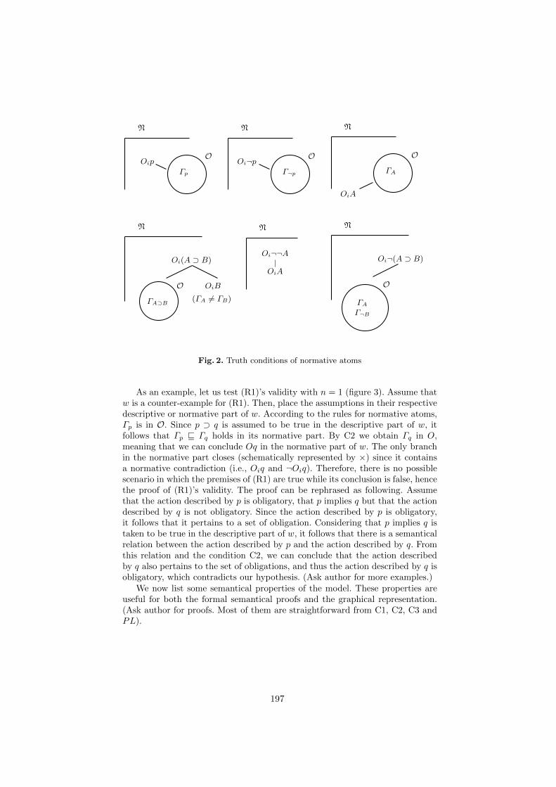
OΓp
N
OipO
Γ¬p
N
Oi¬pO
ΓA
N
OiA
O
ΓAΓ¬B
N
Oi¬(A ⊃ B)
OΓA⊃B
N
Oi(A ⊃ B)
OiB
(ΓA 6= ΓB)
N
Oi¬¬A
OiA
Fig. 2. Truth conditions of normative atoms
As an example, let us test (R1)’s validity with n = 1 (figure 3). Assume thatw is a counter-example for (R1). Then, place the assumptions in their respectivedescriptive or normative part of w. According to the rules for normative atoms,Γp is in O. Since p ⊃ q is assumed to be true in the descriptive part of w, itfollows that Γp v Γq holds in its normative part. By C2 we obtain Γq in O,meaning that we can conclude Oq in the normative part of w. The only branchin the normative part closes (schematically represented by ×) since it containsa normative contradiction (i.e., Oiq and ¬Oiq). Therefore, there is no possiblescenario in which the premises of (R1) are true while its conclusion is false, hencethe proof of (R1)’s validity. The proof can be rephrased as following. Assumethat the action described by p is obligatory, that p implies q but that the actiondescribed by q is not obligatory. Since the action described by p is obligatory,it follows that it pertains to a set of obligation. Considering that p implies q istaken to be true in the descriptive part of w, it follows that there is a semanticalrelation between the action described by p and the action described by q. Fromthis relation and the condition C2, we can conclude that the action describedby q also pertains to the set of obligations, and thus the action described by q isobligatory, which contradicts our hypothesis. (Ask author for more examples.)
We now list some semantical properties of the model. These properties areuseful for both the formal semantical proofs and the graphical representation.(Ask author for proofs. Most of them are straightforward from C1, C2, C3 andPL).
197

w
O
D N
Oipp ⊃ q¬Oiq
Oip¬Oiq
p ⊃ q
¬p q Γp
Γq
Oiq×
Fig. 3. Test of (R1)’s validity
Lemma 8. If ΓA ∈ O, then ΓB⊃A ∈ O for any B.
Lemma 9. If ΓA ∈ O and ΓB ∈ O, then ΓA∧B ∈ O.
Lemma 10. If ΓA∧B ∈ O, then ΓA ∈ O.
Lemma 11. If ΓA ∈ O and ΓA⊃B ∈ O, then ΓB ∈ O.
Lemma 12 (De Morgan). ΓA∧B ∈ O if and only if Γ¬(¬A∨¬B) ∈ O.
Lemma 13. The next lemmas are consequences of (De Morgan) and lemma 8.
If ΓA ∈ O, then ΓA∨B ∈ O (6)
If ΓA ∈ O, then Γ¬(¬A∧¬B) ∈ O (7)
If Γ¬A ∈ O, then Γ¬A∨¬B ∈ O (8)
If Γ¬A ∈ O, then Γ¬(A∧B) ∈ O (9)
If Γ¬(A∨B) ∈ O, then Γ¬A ∈ O (10)
If Γ¬(¬A∨¬B) ∈ O, then ΓA ∈ O (11)
6.2 Soundness of legal inference
In addition to the formal method developed so far, one might want some hintsto test the soundness of a legal inference. Without pretending to be exhaustive,
198

we only give some philosophical insights regarding relevant questions one mighttry to answer. A sound inference is valid and has true (or acceptable) premises.The second question (after the validity test) is thus are the premises true? Thetruth of a normative proposition depends upon the fact that there is an authoritywhich establishes that norm. Hence, one must first contextualize the normativeproposition to a legal authority: is it true according to the Constitution? theCivil Code? the Criminal Code? the Canadian Charter of Rights and Freedom?It is noteworthy that some inferences can be fallacious when the meaning of‘ought’ is not the same throughout the argument.
The context of the argument is also relevant. Consider the premise ‘Paulought to tell the truth’. Assume that ‘ought’ is understood legally. While one isnot legally obliged to tell the truth in one’s day to day life, one is however legallyobliged to tell the truth in a court of justice. It might also be useful to analyze thedescriptive propositions used in conjunction with (R1). The conditional must beanalyzed in terms of necessity and sufficiency. Is the conditional representing asemantical relation of entailment between two actions? Is the action described bythe consequent necessarily entailed by the action described by the antecedent?
Furthermore, one must contextualize the descriptive propositions accordingto the normative authority. For instance, the meaning of the proposition ‘Paulrespects his neighbor’ will vary according to the legal authority. Indeed, themeaning of ‘Paul must respect his neighbor’ will vary depending whether thelegal authority is the Civil Code or the Criminal Code (or the Canadian Charterof Rights and Freedom). When this is done, the question that must be answeredis what legally counts as a lack of respect from the Civil Code’s point of view?In other words, one must answer the question ‘what action counts as A from theauthority’s standpoint?’.13
Now, consider the following argument and assume a context in which premisesP2 and P3 are acceptable. Assume that P1 ‘Paul ought to rescue Peter fromdrowning’, P2 ‘If Paul rescues Peter, then Paul calls 911’ and P3 ‘If Paul calls911, then Paul breaks into Sam’s house’. Therefore, we can conclude that ‘Paulought to break into Sam’s house’. Assuming that breaking and entering is legallyforbidden, this argument leads to a conflict of obligations, hence to a contradic-tion into our current framework. The contradiction can be obtained with theaddition of the premise P0 ‘ Paul ought to not break into Sam’s house’. Butalthough valid, this argument is not sound: either P0 or P1 must be rejected.The conflict of obligations can be overruled with the help of the relation of hi-erarchy since it allows one to prioritize P1 over P0. It is not only likely thatbreaking into Sam’s house to call 911 and save Peter from drowning would notcount as breaking and entering per se, but it is also likely that preserving theintegrity of one’s life would overrule preserving the integrity of one’s property.Hence, premise P0 can be rejected and the conflict of obligations is solved.
A final clue is to consider the principle ought implies can. Replace P2 and P3
in the aforementioned example by P4 ‘If Paul rescues Peter from drowning, thenPaul jumps in the water to retrieve Peter’. From P1 and P4 one can conclude
13 For an analysis of ‘count as’, see [17] and [5].
199

that ‘Paul ought to jump in the water to retrieve Peter’. However, if Paul cannotswim (e.g. if Paul has two broken arms) then the action described by ‘rescuingPeter from drowning’ does not entail the action described by ‘jumping in thewater to retrieve Peter’. Thus, in this context, one could reject premise P2 onthe ground that it is a violation of the ought imply can principle.
200

A Memetic Algorithm for Solving theGeneralized Vehicle Routing Problem
P.C. Pop1, O. Matei2
1 Dept. of Mathematics and Informatics, Technical Univ. of Cluj-Napoca, [email protected]
2 Dept. of Electrical Engineering, Technical University of Cluj-Napoca, [email protected]
Abstract. The generalized vehicle routing problem (GVRP) is one ofthe challenging combinatorial optimization problems that finds a lot ofpractical applications especially in the field of distribution, collectionand logistics. The GVRP is a natural extension of the classical vehiclerouting problem (VRP), obtained by replacing the nodes of a graph withsets of nodes (clusters) and looking for the minimum-cost collection ofroutes subject to capacity restrictions, from a given depot to a number ofpredefined clusters passing through exactly one node from each cluster.This paper describes an efficient memetic algorithm (MA) for solving theGVRP obtained by combining a genetic algorithm (GA) with a powerfullocal search (LS) procedure. The preliminary experiments on benchmarkinstances show that the proposed algorithm compares favorably to allprevious methods.
Keywords: generalized vehicle routing problem, memetic algorithms,genetic algorithms, local search.
1 Introduction
The generalized vehicle routing problem (GVRP) is a natural extension of theclassical vehicle routing problem (VRP) and it was introduced by Ghiani andImprota [3]. The GVRP consists in finding the minimum-cost delivery or collec-tion of routes, subject to capacity restrictions, from a given depot to a numberof predefined clusters passing through one node from each cluster. The problemcan be viewed as a particular type of location-routing problem.
The GVRP has several real world applications mainly in network design.Some applications of the GTSP can be extended naturally to GVRP and severalother situations can be modeled as a GVRP: the post-box collection problem,routing vessels in maritime transportation, health care logistics, the design oftandem configurations for automated guided vehicles, urban waste collectionproblem, survivable telecommunication network design, etc. For a more detaileddescription of the GVRP applications we refer to [1, 2].
The existing literature on the GVRP is rather scarce: Ghiani and Improta[3] showed that the problem can be transformed into a capacitated arc routing
201

problem (CARP) and Baldacci et al. [1] proved that the reverse transformationis valid. Integer programming formulations for the GVRP have been proposedby Bektas et al. [2] and Pop et al. [7].
The difficulty of obtaining optimal solutions for the GVRP has led to thedevelopment of heuristics and metaheuristics: the first such algorithms were theant colony algorithm of Pop et al. [9], the genetic algorithm of Pop et al. [8] andmore recently a branch-and-cut algorithm and an adaptive large neighborhoodsearch proposed by Bektas et al. [2] and an incremental tabu search heuristicdescribed by Moccia et al. [5].
The aim of this paper is to develop an efficient memetic algorithm (MA), ob-tained by combining a genetic algorithm with a powerful local search procedure,for solving the GVRP.
The remainder of the paper is organized as follows. Section 2 formally statesthe GVRP and introduces the corresponding notations. Section 3 recalls the MAmethodology and describes how the GVRP based on the MA framework can besolved. Section 4 presents and analyses the results of the computational exper-iments. The obtained results are compared with the state-of-the-art algorithmsfor solving the GVRP: the branch-and-cut algorithm [2] and the tabu search(TS) heuristic [5]. Finally, the last section concludes the paper.
2 Problem description
Formally, the GVRP is defined on a directed graph G = (V,A) with V =0, 1, 2, ...., n as the set of nodes and the set of arcs A. The set of nodes con-sists of vertex v = 0 which represents the depot and the vertices v = 1, ..., nwhich represent the customers and it is partitioned into k+1 mutually exclusivenonempty subsets, called clusters, V0, V1, ..., Vk (i.e. V = V0 ∪ V1 ∪ ... ∪ Vk andVl ∩ Vp = ∅ for all l, p ∈ 0, 1, ..., k and l 6= p). The cluster V0 is a singletonconsisting of the depot vertex v = 0. The set of arcs is defined by arcs connectingvertices belonging to different clusters called intra-cluster arcs. Inter-cluster arcsdo not exist. A distance dij is associated to each arc (i, j) ∈ A and it representsthe travel cost between vertices i and j. Each customer has a certain amountof demand and the total demand of each cluster can be satisfied via any of itsnodes. There exists m identical vehicles, each with a given capacity Q.
The generalized vehicle routing problem (GVRP) consists in finding the mi-nimum total cost collection of routes starting and ending at the depot, such thateach cluster should be visited exactly once, the entering and leaving nodes ofeach cluster is the same and the sum of all the demands of any route does notexceed the capacity of the vehicle Q.
Therefore the GVRP involves the following two related decisions:
– choosing a node subset S ⊆ V , such that |S ∩ Vi| = 1, for all i = 1, ..., k.
– finding a minimum cost collection of routes in the subgraph of G induced byS, fulfilling the capacity constraints.
202

We will call such a route (i.e. a route visiting exactly one node from a num-ber of clusters and fulfilling the capacity constraints) a generalized route. Anillustrative scheme of the GVRP and a feasible collection of routes is shown inthe next figure.
32
1
4
5
6
7
8
0
9
1011
12
13
route 1
route 3
V1
V2
V3
V4
V5
V6
Figure 1: An example of a feasible solution of the generalized vehicle routingproblem (GVRP)
The GVRP reduces to the classical Vehicle Routing Problem (VRP) when allthe clusters are singletons and to the Generalized Traveling Salesman Problem(GTSP) when Q = ∞.
Concerning the complexity, the GVRP is an NP -hard optimization problembecause it includes the generalized traveling salesman problem as a special case.
3 A memetic algorithm for solving the GVRP
Memetic algorithms have been introduced by Mascato [6] to denote a familyof metaheuristic algorithms that emphasis on the used of a population-basedapproach with separate individual learning or local improvement procedures forproblem search. Therefore a memetic algorithm is a genetic algorithm (GA)hybridized with a local search procedure to intensify the search space.
Genetic algorithms are not well suited for fine-tuning structures which areclose to optimal solutions. Therefore, incorporating of local improvement op-erators into the recombination step of a GA is essential in order to obtain acompetitive GA.
Our effective heuristic algorithm for solving the GVRP is a memetic algo-rithm, which combines the power of genetic algorithm with that of local search.The general scheme of our heuristic is:
203

randomly generatedInitial population
Optimized first
population
duplicate solutions
are eliminated
Population
genetic operators
Non-optimized
population
Optimized
population
local search procedure
local search procedure
duplicate solutions
are eliminated
Surv
ivor
sele
ctio
n
Figure 2: Generic form of our memetic algorithm
3.1 The genetic algorithm
We used a natural, compact and efficient encoding of solutions of GVRP similarto that described by Pop et al. [8]. Specifically, 0 represents the depot and eachcustomer is tagged with a non-duplicated natural number from 1 to n. We repre-sent a chromosome by a variable length array so that the gene values correspondto the nodes selected to form the collection of routes which are delimited by 0representing the depot.
The corresponding chromosome representation of the feasible solution of theGVRP presented in figure 1 is: (3 5 0 6 7 11 0 13), where the values 1, ..., 13represent the customers while the depot denoted by 0 is the route splitter. Route1 begins at the depot then visits customers 3 and 5 belonging to the clusters V1,respectively V2 and returns to the depot. Route 2 starts at the depot and visitsthe customers 6-7-11 belonging to the clusters V3 − V4 − V5. Finally, in route 3only customer 13 from the cluster V6 is visited.
The first step of any genetic algorithm is to generate a set of possible solutionsas an initial generation or population to the problem. Although it seems simple,the convergence, the performance and the ability of the GA are critically affectedby the initial generation.
In the case of the GVRP we carried out experiments with the initial popula-tion generated randomly and with an initial population of structured solutions.The initial population generated randomly has the advantage that is represen-tative from any area of the search space. In order to generate the population ofstructured solutions we used a Monte Carlo based method. Based on computa-tional experiments we observed that this method assures an initial populationwith a average fitness with 20% better than a population generated entirely ran-domly, but the major drawback was that such a population lacks the diversityneeded to obtain near-optimal solutions.
204

Analyzing the advantages and disadvantages of these ways to generate theinitial population and based on computational experiments we decided to choosethe initial population randomly.
In order for genetic algorithms to work effectively, it is necessary to be able toevaluate how ”good” a potential solution is relative to other potential solutions.In our case, the fitness value of a feasible solution, i.e. collection of routes, isgiven by the sum of the costs of the arcs selected in the routes. The aim is tofind the minimum cost collection of routes.
The crossover operator requires some strategy to select two parents fromprevious generation. We used in our algorithm an elitist approach: the parents arechosen randomly between the best 40% (parameter chosen based on preliminaryexperiments) of all the solutions in the previous generation. We select randomlytwo chromosomes from the best 40% of the all the solutions of the previousgeneration, assign the cheapest (w.r.t. cost minimization) to parent 1 and repeatthe procedure to select parent 2.
Offspring are produced from two parents using the following 2-point orderstandard crossover procedure: it creates offspring which preserve the order andposition of symbols in a subsequence of one parent while preserving the relativeorder of the remaining symbols from the other parent. It is implemented byselecting two random cut points which define the boundaries for a series ofcopying operations. First, the symbols between the cut points are copied fromthe first parent into the offspring. Then, starting just after the second cut-point,the symbols are copied from the second parent into the offspring, omitting anysymbols that were copied from the first parent. When the end of the secondparent sequence is reached, this process continues with the first symbol of thesecond parent until all the symbols have been copied into the offspring. Thesecond offspring is produced by swapping round the parents and then using thesame procedure.
Next we present the application of the proposed 2-point order crossover in thecase of the problem presented in fig. 1. We assume two well-structured parentschosen randomly, with the cutting points between nodes 2 and 3, respectively 5and 6:
P1 = (13 0 | 3 5 0 | 11 7 6) P2 = (4 2 | 13 0 11 | 10 6)
Note that the length of each individual differs according to the number ofroutes. According to figure 1, the cluster representation of the parents is asfollows:
C1 = (6 0 | 1 2 0 | 5 4 3) C2 = (2 1 | 6 0 5 | 4 3)
The sequences between the two cutting-points are copied into the two off-spring:
O1 = (x x | 3 5 0 | x x x) O2 = (x x | 13 0 11 | x x)
The nodes of the parent P1 are copied into the offspring O2 if O2 does notcontain already nodes in the same clusters as the nodes of P1. The sequenceof the nodes of P1 is 13 − 0 − 3 − 5 − 0 − 11 − 7 − 6, and the clusters are
205

6 − 0 − 1 − 2 − 0 − 5 − 4 − 3. Note that the cluster 6 is already representedin O2 by the node 13 and the cluster 5 by the node 11. The depot (0) is keptany way as it is a splitter. Therefore the remaining sequence of nodes in P1 is0−3−5−0−7−6. Therefore the offspring O2 is: O2 = (0 3 | 13 0 11 | 5 0 7 6).
Then the nodes of the parent P2 are copied into the offspring O1 in thesame manner. The nodes of the clusters not present in O1 are copied into theremaining positions: O1 = (13 0 | 3 5 0 | 11 10 6).
Mutation is a genetic operator that alters one ore more gene values in achromosome from its initial state. This can result in entirely new gene valuesbeing added to the gene pool. With these new gene values, the genetic algorithmmay be able to arrive at better solution than was previously possible.
We use in our GA two random mutation operators: the first one (intra-routemutation) selects randomly a cluster to be modified and replaces its currentnode by another one randomly selected from the same cluster and the secondone (inter-route mutation) is a swap operator, it picks two random locations inthe solution vector and swaps their values. The new chromosome is accepteddirectly if it results in a feasible GVRP, otherwise the route that exceeds thevehicle capacity is decomposed into several ones as describe before.
The selection process is deterministic. In our algorithm we use the (µ + λ)selection, where µ parents produce λ offspring. The new population of (µ + λ)is reduced again to µ individuals by a selection based of the ”survival of thefittest” principle. In other words, parents survive until they are suppressed bybetter offspring. It might be possible for very well adapted individuals to surviveforever.
The genetic parameters are very important for the success of a GA, equallyimportant as the other aspects, such as the representation of the individuals, theinitial population and the genetic operators. The most important parametersare: the population size µ has been set to 2 times the number of the clusters,the intermediate population size λ was chosen twice the size of the population:λ = 2 · µ and the mutation probability was set at 10%.
The loop of chromosome generations is terminated when certain conditionsare met. When the termination criteria are met, the elite chromosome is returnedas the best solution found so far. In our algorithm we used the terminationcondition based on the number of generations, namely 104 generations seemsnecessary to sufficiently explore the solution space.
3.2 Local improvement procedure
Classical GAs are not aggressive enough for some combinatorial optimizationproblems. One possibility to obtain more competitive heuristics is to combinethe GAs with local search procedures.
For each solution belonging to the current generation we use a local improve-ment procedure that runs several local search heuristics sequentially. Once animprovement move is found, it is immediately executed. In our algorithm weused the following local search heuristics:
206

– 2-opt intra-route moves: consist of eliminating any two non-adjacent edgesin each of the routes of the solution and reconnect the two resulting pathsin a different way to obtain a different route. An improvement is obtainedif the cost of the new collection of routes is less than the cost of the initialcollection of routes. The heuristic applies all the improvements found.
– Cluster route optimization (CO): uses the shortest path algorithm to findthe best node from each cluster when the order of visiting the clusters isgiven.Given a collection of r global routes of form (V0, Vk1
, ..., Vkp) in which the
clusters are visited, we show that the best feasible route R∗ (w.r.t cost min-imization), i.e. a collection of r generalized routes visiting the clusters ac-cording to the given sequence can be done in polynomial time, by solvingthe following r shortest path problems.For each sequence of visiting the clusters (V0, Vk1
, ..., Vkp), the best gener-
alized route visiting the clusters according to the given sequence can bedetermined in polynomial time by constructing a layered network (LN) withp+ 2 layers corresponding to the clusters V0, Vk1
, ..., Vkpand in addition we
duplicate the cluster V0. The layered network contains all the nodes of theclusters V0, Vk1
, ..., Vkpplus an extra nodes 0′ ∈ V0.
V0
V
V Vk
Vk
k
V0
1
2
p
...
Fig. 3: Example showing a route visiting the clusters V0, Vk1, ..., Vkp
in theconstructed layered network LN
We consider paths from 0 to 0′, 0′ ∈ V0, that visits exactly one node fromeach cluster Vk1
, ..., Vkp, hence it gives a feasible generalized route. Con-
versely, every generalized route visiting the clusters according to the sequence(V0, Vk1
, ..., Vkp) corresponds to a path in the layered network from 0 ∈ V0
to 0′ ∈ V0.Therefore, it follows that the best (w.r.t cost minimization) collection ofroutes R∗ can be found by determining r shortest paths from 0 ∈ V0 to thecorresponding 0′ ∈ V0 with the property that visits exactly one node fromeach of the clusters (Vk1
, ..., Vkp).
– Neighborhood cross (NC): this neighborhood includes all feasible solutionsobtained by the replacement of two arc by other two. Given two differentroutes r1 and r2, an arc is deleted from each of them dividing the routes intotwo components that are combined such that a new route is made of thefirst component of r1 and the second of r2 and another new route is madeof the first component of r2 and the second component of r1.
207

V0V0
Vp
Vq
Vi
Vj
Vj
Vi
Vp
Vq
Fig. 4. An example of a possible string cross
– Neighborhood exchange (NE): two strings of at most k vertices are exchangedbetween two routes. A new solution is obtained from the current one byselecting k vertices from one route and exchanging them with k verticesbelonging to another route. The exchange is acceptable only if it produces afeasible solution.
V0V0
Vp
Vq
Vi
Vj
Vq
Vp
Vi
Vj
Figure 5: An example of a possible string exchange for k = 1
– Neighborhood relocation (NR): a string of at most k vertices is moved fromone route to another (k = 1 or k = 2). This neighborhood includes all feasiblesolutions obtained by deleting one or two vertices from their route r1 andinserting them into a route r2.
V0V0
Figure 6: An example of a possible string relocation
Our improvement procedure applies all the described local search heuristicscyclically.
4 Computational results
In order to asses the performance of our proposed memetic algorithm for solv-ing the GVRP, we conducted our experiments on a set of instances generated
208

through an adaptation of the existing instances in the CVRP-library availableat http://branchandcut.org/VRP/data/. The naming of the generated instancesfollows the general convention of the CVRP instances available online, and fol-lows the general format X − nY − kZ −CΩ − V Φ, where X corresponds to thetype of the instance, Y refers to the number of vertices, Z corresponds to thenumber of vehicles in the original CVRP instance, Ω is the number of clustersand Φ is the number of vehicles in the GVRP instance. These instances were usedby Bektas et al. [2] and Moccia et al. [5] in their computational experiments.
We considered for our instances as in [2, 5] two clustering procedures one withθ = 2 and the other one with θ = 3. However, the solution approach proposedin this paper is able to handle any cluster structure.
The testing machine was an Intel Dual-Core 1,6 GHz and 1 GB RAM. Theoperating system was Windows XP Professional. The algorithm was developedin Java, JDK 1.6.
In Tables 1 and 2, we summarize the results of all methods on a set of 30 testsmall to medium instances with θ = 2 and θ = 3. The first column in the tablesgive the name of the instances, the second column provides the values of the bestlower bounds in the branch-and-cut tree [2]. Next three columns contains the val-ues of the best solutions obtained using the adaptive large neighborhood search(ALNS) [2], the incremental tabu search (ITS) [5] and our memetic algorithm.
Table 1. Computational results on smalland medium instances with θ = 2
Instance LB [2] ALNS [2] ITS [5] MA
A-n32-k5-C16-V2 519 519 519 519A-n34-k5-C17-V3 489 489 489 489A-n38-k5-C19-V3 476 476 476 476A-n45-k6-C23-V4 613 613 613 613A-n63-k9-C32-V5 900.3 912 912 908
B-n31-k5-C16-V3 441 441 441 441B-n34-k5-C17-V3 472 472 472 472B-n38-k6-C19-V3 451 451 451 451B-n45-k5-C23-V3 497 497 497 497B-n63-k10-C32-V5 816 816 816 816
P-n16-k8-C8-V5 239 239 239 239P-n20-k2-C10-V2 154 154 154 154P-n21-k2-C11-V2 160 160 160 160P-n22-k2-C11-V2 162 162 162 162P-n55-k15-C28-V8 545.3 555 565 558
Table 2. Computational results on smalland medium instances with θ = 3
Instance LB [2] ALNS [2] ITS [5] MA
A-n32-k5-C11-V2 386 386 386 386A-n33-k5-C11-V2 315 318 315 315A-n34-k5-C12-V2 419 419 419 419A-n38-k5-C13-V2 367 367 367 367A-n63-k9-C21-V3 625.6 642 643 642
B-n31-k5-C11-V2 356 356 356 356B-n34-k5-C12-V2 369 369 369 369B-n35-k5-C12-V2 501 501 501 501B-n45-k5-C15-V2 410 422 410 410B-n50-k7-C17-V3 393 393 393 393
P-n16-k8-C6-V4 170 170 170 170P-n19-k2-C7-V1 111 111 111 111P-n20-k2-C7-V1 117 117 117 117P-n40-k5-C14-V2 213 213 213 213
P-n50-k10-C17-V4 292 292 292 292
From the summary Tables 1 and 2, we can observe that our memetic algo-rithm performs slightly better in comparison to all other approaches for solvingthe considered both small and medium size instances. In one instance P-n55-k15-C28-V8 the solution returned by our algorithm exhibits a gap of 0.01 %with the best known solution provided by the ALNS and for the rest of the in-stances for which the optimal solution is known we solved them optimally withour algorithm.
Regarding the computational times, it is difficult to make a fair comparisonbetween algorithms, because they have been evaluated on different computersand they are implemented in different languages. The running time of our MAis proportional with the number of generations. From the computational exper-
209

iments, it seems that 104 generations are enough to explore the solution spaceof the GVRP. Our proposed heuristic algorithm seems to be slower than ALNSand comparable with ITS. Therefore we can conclude that our approach will beappropriate when the execution speed is not critical.
5 Conclusions
In this paper, we developed a memetic algorithm for solving the GVRP. The pro-posed heuristic integrates a number of original features: we combine a geneticprogramming with a powerful local search procedure, our local search proce-dure consists of five local search heuristics, their diversity and power being animportant factor for solving successfully the GVRP.
The preliminary experimental results show that our algorithm is robust andcompares favorably with all known heuristic approaches to the problem in termsof solution quality. In the future, we plan to asses the the generality and scala-bility of the proposed hybrid heuristic by testing it on more instances.
Acknowledgments. This work was supported by a grant of the RomanianNational Authority for Scientific Research, CNCS - UEFISCDI, project numberPN-II-RU-TE-2011-3-0113.
References
1. Baldacci, R., Bartolini, E., Laporte, G.: Some applications of the generalized vehiclerouting problem. Journal of the Operational Research Society, 61 (7), 1072-1077(2010)
2. Bektas, T., Erdogan, G., Ropke, S.: Formulations and Branch-and-Cut Algorithmsfor the Generalized Vehicle Routing Problem. Transportation Science, 45(3), 299-316 (2011)
3. Ghiani, G., Improta, G.: An efficient transformation of the generalized vehicle rout-ing problem. European Journal of Operational Research, 122, 11-17 (2000)
4. Fischetti, M., Salazar, J.J, Toth, P.: A branch-and-cut algorithm for the symmetricgeneralized traveling salesman problem. Operations Research, 45, 378-394 (1997)
5. Moccia, L., Cordeau, J-F., Laporte, G.: An incremental neighborhood tabu searchheuristic for the generalized vehicle routing problem with time windows. Journal ofthe Operational Research Society, 63(2), 232-244 (2012)
6. Moscato, P.: On Evolution, Search, Optimization, Genetic Algorithms and MartialArts: Towards Memetic Algorithms. Caltech Concurrent Computation Program,Report 826 (1989)
7. Pop, P.C., Kara, I., Horvat Marc, A.: New Mathematical Models of the GeneralizedVehicle Routing Problem and Extensions, Applied Mathematical Modelling, 36(1),97-107 (2012)
8. Pop, P.C., Matei, O., Pop Sitar, C., Chira, C.: A genetic algorithm for solving thegeneralized vehicle routing problem. Lecture Notes in Artificial Intelligence, 6077,119-126 (2010)
9. Pop, P.C., Pintea, C., Zelina, I., Dumitrescu, D.: Solving the Generalized VehicleRouting Problem with an ACS-based Algorithm. American Institute of Physics,1117, 157-162 (2009)
210
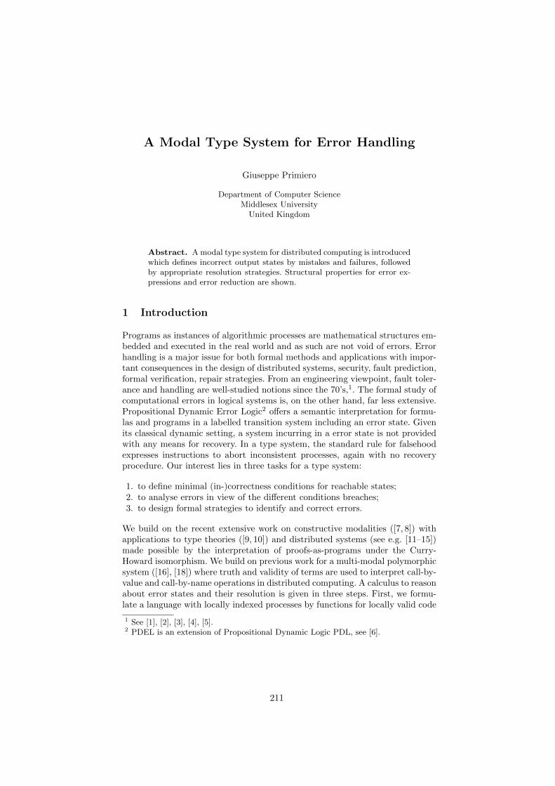
A Modal Type System for Error Handling
Giuseppe Primiero
Department of Computer ScienceMiddlesex University
United Kingdom
Abstract. A modal type system for distributed computing is introducedwhich defines incorrect output states by mistakes and failures, followedby appropriate resolution strategies. Structural properties for error ex-pressions and error reduction are shown.
1 Introduction
Programs as instances of algorithmic processes are mathematical structures em-bedded and executed in the real world and as such are not void of errors. Errorhandling is a major issue for both formal methods and applications with impor-tant consequences in the design of distributed systems, security, fault prediction,formal verification, repair strategies. From an engineering viewpoint, fault toler-ance and handling are well-studied notions since the 70’s,1. The formal study ofcomputational errors in logical systems is, on the other hand, far less extensive.Propositional Dynamic Error Logic2 offers a semantic interpretation for formu-las and programs in a labelled transition system including an error state. Givenits classical dynamic setting, a system incurring in a error state is not providedwith any means for recovery. In a type system, the standard rule for falsehoodexpresses instructions to abort inconsistent processes, again with no recoveryprocedure. Our interest lies in three tasks for a type system:
1. to define minimal (in-)correctness conditions for reachable states;2. to analyse errors in view of the different conditions breaches;3. to design formal strategies to identify and correct errors.
We build on the recent extensive work on constructive modalities ([7, 8]) withapplications to type theories ([9, 10]) and distributed systems (see e.g. [11–15])made possible by the interpretation of proofs-as-programs under the Curry-Howard isomorphism. We build on previous work for a multi-modal polymorphicsystem ([16], [18]) where truth and validity of terms are used to interpret call-by-value and call-by-name operations in distributed computing. A calculus to reasonabout error states and their resolution is given in three steps. First, we formu-late a language with locally indexed processes by functions for locally valid code
1 See [1], [2], [3], [4], [5].2 PDEL is an extension of Propositional Dynamic Logic PDL, see [6].
211

and global values: errors can arise in executing them at locations where they arenot valid. Second, we enrich the language with the means for mobility of termsand code via modal-style functions, for global and local validation from and toaddresses: then errors can arise in fetching and sending data at wrong locations.Finally, we internalize these two main kinds of errors: functions for mistakes asconceptual, semantic or syntactic errors; and functions for failures as procedural,mobility-related errors.3
2 ML♦err: A Type System with Error States
ML♦err is a modal type system for mobile distributed programming with errorstates and handling procedures, inspired by an extension of a standard Martin-Lof type theory with judgemental modalities, avoiding dependent types.
Definition 1 (Syntax). The syntax of ML♦err is defined by the following al-phabet:
Programs Π := xi | ai, for i ∈ I
Specifications Σ := α | ⊥ | α× β | α+ β | α→ β | α ⊃ βLocations I := 1 < · · · < nOperations Φ := exec(α) | runi(α) | runi∪j(α · β) | runi∩j(α · β)| synchroj(β(exec(α))), where · ∈ +,×Error Functions H := fail@i(τ) | mistake(τ)Concurrency Functions C := access@i(t :τ \ ⊥) | φ(τ)WITH(Π ∪ I ∪ Γ ),φ ∈ ΦData Stacks (Contexts) := Γi, ∆i | iΓ, ∈ ,♦Remote Operations := GLOB(i∪jΓ, α) | BROAD(♦i∩jΓ, α)Portable Code := RET (Γi∪j , α) | SEND(Γi∩j , α)
Program terms (Π) include variables (xi) to refer to local code and constants(ai) to refer to globally safe values. Indices (I) collect strictly ordered locationsfor execution of programs in a network. Types of programs (Σ) are output val-ues defined recursively from the atomic type α using ‘connectives’ as functions.Local codes and global values define the two main operations in Φ by rule con-structions: exec(α) is the output value generated by constant construction, isglobally valid and can be called by name; runi(α) is the local output value ati generated by variable construction, is locally bounded and can only be calledby value. Compound code execution at ordered intersection of locations i ∩ jis given by ×; at union of locations i ∪ j by +; code functional composition(⊃) composes the outputs of two derivable run to their intersection at loca-tions; values composition (→) transforms a local run and a global exec intoeach other; synchro associates a value of a run with an exec function. Contextsexpress data stacks for program execution with valid code (true assumptions)Γi := runi(α), . . . , runi(ν) | x1 : α, . . . , yi : ν and safe values (valid assump-tions) ∆i := exec(α), . . . , exec(ν) | a1 : α, . . . , ni : ν. Modal contexts express
3 This formal treatment is based on the taxonomy of errors for information systemswith procedural semantics introduced in [17].
212

the occurrence of run and exec functions: iΓ = exec(α) | for all ai :α ∈ Γ isobtained from a stack of safe values only, and iΓ ` α declares code correctnessof value α with complete instructional informations at run-time in Γ , all availablefrom i but valid at any other location accessible from i; ♦iΓ = i(α) | ∈ Φis inferred from a stack of valid code so that ` runi(α) for at least one xi :α ∈ Γ ,and ♦iΓ ` α declares code correctness of value α with complete instructionalinformations at run-time in Γ , accessible only locally at i. Mobility rules areadded in the form of introduction and elimination rules for transmission opera-tors that allow to express at which reachable locations in a network a programexecutes and terminates. GLOB works as a remote procedure call for safe valueswith RET as the corresponding declaration of portable value; BROAD is theremote procedure call for valid code, with SEND the corresponding portablerule. Concurrency functions C include: access as a command for program (t ∈ Π)accessibility at a location; and function execution (φ ∈ Φ) on values (τ ∈ Σ) with(WITH) an indexed, eventually compound program. Error functions H includefailures for syntax errors on local processes and mistakes for semantic errorsglobal on a specification.
Definition 2 (Typing Rules). The set of typing rules for execution and mo-bility of code and values is:
Global∆i, ai :α ` exec(α)
∆i, ai :α ` exec(α)@I
∆i ` access@i(a :α)
∆i;Γi ` access@i(a :α)@E
∆i;Γi, xi :α ` runi(α)
∆i;Γi ` φ(α)WITH-I
∆i ` φ(α)WITH(t, Γ )
∆i ` φ(α)WITH(t, Γ ) ∆i;Γ ` t :αWITH-E
∆i;Γ, t :α ` φ(α)
ai :α ` exec(α) bj :β ` exec(β)I×
` runi∩j(α× β)
` runi∩j(α× β)E1×
` exec(α)` runi∩j(α× β)
E2×` exec(β)
ai :α ` exec(α)I + (l)
` runi(α+ β)
bj :β ` exec(β)I + (r)
runj(α+ β)
` runi∪j(α+ β) runi(α) ` ck :γ runj(β) ` ck :γE+
` runi∩j∩k(γ)
` runi(α) xi :α ` runj(β)I ⊃
runi∩j(α ⊃ β)` runi∩j(α ⊃ β) xi :α
E ⊃xi :α ` runj(β)
` exec(α) ai :α ` exec(β)I →` runi∪j(α→ β)
` runi∪j(α→ β) ai :αE →
exec(α) ` exec(β)
` runi∩j(α ⊃ β) ai :αSynchro
` synchroj(β(exec(α)))
213

Γi, xj :α ` runj(α) iΓ, xj(aj) : α ` exec(α)RPC1
GLOB(i∪jΓ, α)
Γi, xj :α ` runj(α) ♦iΓ ` runj(α)RPC2
BROAD(♦i∩jΓ, α)
iΓ, aj :α ` exec(α) GLOB(i∪jΓ, α)PORT1
RET (Γi∪j , α)
iΓ, xj :α ` runi∩j(α) BROAD(♦i∩jΓ, α)PORT2
SEND(Γi∩j , α)
Global generates an output value under valid assumptions or safe values.The @-operator tells how to access and run locally code for which safe value isavailable. The other concurrency function WITH simply associate the run orexec function on value with the required program term and stack. Connectives+,× work as expected with values and codes. An instance of I⊃ with runi(α)and xi(α) ` runj(α), allows to move from runi to runi∩j . To move from runi toruni∪j , one needs the intermediate step of obtaining an exec(α) from runi(α),thus inducing runi∪j(α→ α). RPC1 says that if all valid code for the executionof a program of type α is available, then α is globally valid with the relevant stack.The corresponding elimination PORT1 starts from a similarly derived value todecompose its valid locations. RPC2 says that if execution at i of a program forα requires code bounded to address j, then resources at the intersection of i, jare needed for any execution. The corresponding elimination PORT2 starts froma similarly derived valid code to infer its variable constructor for local validityof α. Error states are obtained either by a syntax error at execution of a validprogram; or by a semantic error related to the (possibly correct) execution of aprogram. Both induce an invalid 〈ti, τ〉 | t ∈ Π; i ∈ I; τ ∈ Σ pair. Error functionshave the following intended meaning:
– fail@i(τ) is the state of the system where a program t :τ \⊥ induces a failurewhen accessed at index i;
– mistake(τ) is the state of the system where reference to specification τinduces an error.
Because φ does not range over H in WITH, the mistake function will not iterate.Similarly, in access@, the term t cannot be typed in ⊥. This is required to obtainerror reducibility formulated by Theorem 4.
2.1 Mistakes
Mistakes are semantic errors caused by missing resources for a given pair 〈ti, τ〉.In the following, we consider two formulations, with respectively φ := (exec) andφ := (runi). In the first case, the system refers to a τ ∈ Σ for which no runningt ∈ Π has been defined. This is for example the case of a program that includesin its specification design a sub-process for which no routine has been defined.Consequently, any further specification υ depending on τ will induce an errorstate.
214

∆i;Γi ` runi(τ → ⊥) ∆i; xi :τ ` runi(υ)Mistake1
Γi;∆i ` mistake(exec(υ)WITH(τ))
In the second case, given a τ ∈ Σ, the corresponding t ∈ Π is not reducible toany other valid one in the system. This is the case where a routine for the calledspecification exists, but is ill-defined. Correspondingly, matching any υ with anyrunning t is ill-defined.
∆i;Γi ` runi(t ⊃ ⊥) Γi, xi :τ ` runi(υ)Mistake2
Γi;∆i ` mistake(runi(υ)WITH(ti))
2.2 Failures
Failures are syntax errors related to the use, accessibility and retrieval of physicalresources. To reason about them we use the access@i function and generatefailure of mobility rules. The first case of failure is given by a program accessingwrong resources (possibly at the right location). An example would be the choiceof inappropriate procedural steps, like rules in a logical derivation. In this casewe consider mobility rules for overall safe code that do not call upon the requiredresources. The operation involved is PORT1:
iΓ, tj :τ ` exec(υ) GLOB(i∪jΓ, τ)FailPort1iΓ, access@j(t
′ : τ ′) ` fail@i∪j(υ) (t′ 6= t; τ ′ 6= τ)
The first premise declares the required resources, the second the allowed mobility,while the conclusion states failure in view of renamed resources. Computation-ally, this rule is very expensive: to be complete it requires declaration for everyt′ : τ ′ that does not reduce to tj :τ .
The other case of failure is caused by programs accessing (possibly correct)data at wrong locations. It satisfies cases of failing calls on local resources. Werefer here to program execution where code mobility is not overall safe in remoteprocedure calls and code portability. The rule involved is RPC2:
iΓ ; xj :τ ` runi∩j(υ) BROAD(♦i∩jΓ, τ)FailPort2♦iΓ, access@k>j(t :τ) ` fail@i∩j(υ)
The first premise declares the required local resources, the second the allowedmobility, while the conclusion states failure in view of non-accessible locations.
3 Error Handling Mechanisms
For each error and failure function rule, we define an appropriate handling mech-anism.
Γi ` mistake(exec(υ)WITH(τ)) Γi, tj :τ′ ` exec(τ ′)
HandleMistake1Γi ` synchroj(υ(exec([τ/τ ′])))
Γi ` mistake(runi(υ)WITH(ti)) Γi, [ti/xj ] :τ ` runi(υ)HandleMistake2
Γi ` runj∩i(τ ⊃ υ)
215
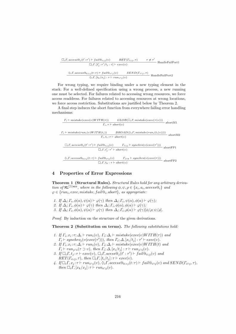
iΓ, access@j(t′ :τ ′) ` fail@i∪j(υ) RET (Γi∪j , τ) τ 6= τ ′
HandleFailPort1iΓ, [t′j :τ′/tj : τ ] ` exec(υ)
♦iΓ, access@k>j(t :τ) ` fail@i∩j(υ) SEND(Γi∩j , τ)HandleFailPort2♦iΓ, [tk/xj ] : τ ` runi∩j(υ)
For wrong typing, we require binding under a new typing element in thestack. For a well-defined specification using a wrong process, a new runningone must be selected. For failures related to accessing wrong resources, we forceaccess readdress. For failures related to accessing resources at wrong locations,we force access restriction. Substitutions are justified below by Theorem 2.
A final step induces the abort function from everywhere failing error handlingmechanisms:
Γi ` mistake(exec(υ)WITH(τ)) GLOB(iΓ,mistake(exec(τ(υ)))abortM1
Γi, τ ` abort(υ)
Γi ` mistake(runi(υ)WITH(ti)) BROAD(♦iΓ,mistake(runi(ti(υ))))abortM2
Γi, ti :τ ` abort(υ)
iΓ, access@j(t′ :τ ′) ` fail@i∪j(υ) Γi∪j ` synchro(υ(exec(τ ′)))
abortFP1iΓ, t′j :τ′ ` abort(υ)
♦iΓ, access@k>j(t :τ) ` fail@i∩j(υ) Γi∩k ` synchro(υ(exec(τ)))abortFP2iΓ, tk : τ ` abort(υ)
4 Properties of Error Expressions
Theorem 1 (Structural Rules). Structural Rules hold for any arbitrary deriva-tion of ML♦err, where in the following φ, ψ, ρ ∈ xi, ai, access@i andϕ ∈ runi, exec,mistake, fail@i, abort, as appropriate:
1. If ∆i;Γi, φ(α), ψ(α) ` ϕ(γ) then ∆i;Γi, ψ(α), φ(α) ` ϕ(γ);2. If ∆i;Γi, φ(α) ` ϕ(γ) then ∆i;Γi, φ(α), φ(α) ` ϕ(γ);3. If ∆i;Γi, φ(α), ψ(α) ` ϕ(γ) then ∆i;Γi, ρ(α) ` ϕ(γ)[φ/ρ;ψ/ρ].
Proof. By induction on the structure of the given derivations.
Theorem 2 (Substitution on terms). The following substitutions hold:
1. If Γi, xi :τ ;∆i ` runi(υ), Γi;∆i ` mistake(exec(υ)WITH(τ)) andΓi ` synchroj(υ(exec(τ ′))), then Γi;∆, [xi/tj ] : τ ′ ` exec(υ).
2. If Γi, xi :τ ;∆i ` runi(υ), Γi;∆i ` mistake(exec(υ)WITH(t) andΓi ` runj∩i(τ ⊃ υ), then Γi;∆, [xi/tj ] : τ ` runj∩i(υ).
3. If iΓ, tj :τ ` exec(υ), iΓ, acess@j(t′ : τ ′) ` fail@i∪j(υ) and
RET (Γi∪j , τ), then iΓ, [ti/tj ] :τ ` exec(υ).4. If iΓ, xj :τ ` runi∩j(υ), ♦iΓ, access@k>j(t :τ) ` fail@i∩j(υ) and SEND(Γi∩j , τ),
then iΓ, [xk/xj ] :τ ` runi∩j(υ).
216

Proof. By induction on the relevant derivation, using the structure of the mistakeor failure rule.
Error functions and their handling rules can be seen as respectively intro-duction and elimination rules for fail and mistake. To show that these aremeaningful in a logical sense, detours obtained by the error introduction and itshandling should generate a valid expression which would hold without errors.This proves local soundness.
∆i; xi :τ ` runi(τ) exec(τ) ` ⊥→-I
∆i ` runi(τ → ⊥) ∆i, xi :τ ` runi(υ)M1
∆i;Γi ` mistake(exec(υ)WITH(τ) Γi, tj :τ′ ` exec(τ ′)
HM1Γi;∆i ` synchroj(υ(exec(τ ′)))
Γi, xj :τ′ ` runi∩j(τ
′ ⊃ υ) ∆i ` tj :τ ′Synchro
Γi;∆i ` synchroj(υ(exec(τ ′)))
Γi; xi :τ ` runi(τ) runi(τ) ` ⊥ ⊃-IΓi ` runi(τ ⊃ ⊥) Γi, xi :τ ` runi(υ)
M2Γi ` mistake(runi(υ)WITH(ti) Γi, xj :τ ` runi(υ)
H2Γi ` runj∩i(τ ⊃ υ)
Γi ` runj(τ) Γi, xj :τ ` runi(υ)I⊃
Γi ` runj∩i(τ ⊃ υ)
Γi ` access@i(t :τ)@E
Γi, xi :τ ` runi(τ) iΓ, xi/ti :τ ` exec(τ)RPC1
GLOB(i∪jΓ, τ)FP1iΓ, access@i(t
′ : τ ′) ` fail@i∪j(τ) RET (Γi∪j , τ)HFP1iΓ, ti :τ ` exec(τ)
Γi ` ti :τGlobaliΓ, ti :τ ` exec(τ)
∆i, ti :τ ` exec(τ)@I
∆i ` access@i(τ) ∆i, xi :τ ` runi(τ)RPC2
BROAD(♦i∩jΓ, τ)FP2♦iΓ, access@j>i(t : τ) ` fail@i∩j(τ) SEND(Γi∪j , τ)
HFP2♦iΓ, xj :τ ` runi∩j(τ)
Γi ` runi(τ) xi :α ` runj(τ)I⊃♦iΓ, xi :τ ` runi∩j(τ)
217

Definition 3 (βerr). The following resolve reductions hold in view of local sound-ness shown above:
1. ∆i;Γi ` mistake(exec(υ)WITH(τ)) and Γi, tj : τ ′ ` exec(τ ′) βerr
−−→ ∆i;Γi `synchro(υ(exec([τ/τ ′])));
2. Γi ` mistake(runi(υ)WITH(ti) and Γi, xj :τ ` runi(υ)βerr
−−→ Γi ` runj∩i([ti/tj ] :τ ⊃ υ);
3. iΓ, access@i(t′ : τ ′) ` fail@i∪j(τ) and RET (Γi∪j , τ)
βerr
−−→ iΓ, [t′i/ti] `exec(τ);
4. ♦iΓ, access@j>i(t :τ) ` fail@i∩j(t :τ) and SEND(Γi∪j , τ)βerr
−−→ ♦iΓ, [ti/xi] :τ ` runi∩j(τ).
The appropriate counterparts are expansions obtained by eliminations fol-lowed the relevant introductions, to show that handle-rules are not too weak.This proves local completeness.
GLOBΓi, tj :τ
′ ` exec(τ ′) Γi ` mistake(exec(υ)WITH(τ)HM1
Γi ` synchroj(υ(exec(τ ′)))@I
Γi ` access@j(τ′)
@E∆i;Γi, xj :τ
′ ` runj(τ′) ∆i;Γi ` runi(τ → ⊥)
M1∆i;Γi ` mistake(exec(υ)WITH(τ))
Γi ` access@i(t :τ)@E
Γi, xj :τ ` runi(τ′) Γi ` mistake(runi(υ)WITH(ti)
HM2Γi ` runj∩i(τ ⊃ υ) ⊃ EΓi, xj :τ ` runi(υ) Γi ` runi(t→ ⊥)
M2∆i;Γi ` mistake(runi(υ)WITH(ti))
PORT1RET (Γi∪j , τ) iΓ, access@j(t
′ :τ) ` fail@i∪j(υ)HFP1iΓ, tj :τ ` exec(υ) GLOB(i∪jΓ, υ)
FP1iΓ, access@j(t′ :τ ′) ` fail@i∪j(υ)
PORT2SEND(Γi∩j , τ) ♦iΓ, access@k>j(t :τ) ` fail@i∩j(υ)
HFP2iΓ, xj :τ ` runi∩j(u :υ) BROAD(♦i∩jΓ, υ)FP2♦iΓ, access@j>i(t :τ) ` fail@i∩j(υ)
Definition 4 (ηerr). The following error expansions hold in view of the localcompleteness shown above:
1. ∆i, run(τ → ⊥) ` runi(υ)ηerr−−→ ∆i;Γi ` mistake(exec(υ)WITH(τ);
2. Γi, runi(t ⊃ ⊥) ` runi(υ)ηerr−−→ ∆i;Γi ` mistake(runi(υ)WITH(ti);
218

3. iΓ,GLOB(i∪jΓ, τ) ` runi∪j(υ)ηerr−−→ iΓ, access@j(t
′ :τ ′) ` fail@i∪j(u :υ);
4. iΓ,BROAD(♦i∩jτ) ` runi∩j(υ)ηerr−−→ ♦iΓ, access@k>j(t : τ) ` faili∩j(u :
υ).
In the following, we use respectively ERR for an expression obtained byM1,M2, FP1 or FP2; and RES for one obtained by HM1, HM2, HFP1 orHFP2:
Theorem 3 (Error Reduction and Expansion). Subject reduction and ex-pansion for error expressions hold as follows:
– If ∆i;Γi ` ERR and ERRβerr
−−→ RES, then ∆i;Γi ` RES.
– If ∆i;Γi ` ERR and ERRηerr−−→ ERR′, then ∆i;Γi ` ERR′.
Proof. Forβerr
−−→, use substitution properties on the relevant expression of RES.
Forηerr−−→, reconstruct the derivation of ERR′.
β-reduction reduces ERR-expressions to RES-expressions, possibly after a finite
number ofηerr−−→ operations, until it cannot be longer reduced to a sub-expression
of error-type. This is called an irreducible resolution expression, which can stillcontain a traditional redex of a non-error type.
Theorem 4 (Irreducible RES-expression). If ∆i;Γi ` ERR and ERRβerr
−−→RES and there is no RES′ such that RES
βerr
−−→ RES′, then RES is an irre-ducible resolution expression.
Proof. The proof proceeds by error reduction. By inversion, consider the lastinference step (error rule) in the derivation. Because RES has no further errorreduction available, it will be obtained by one of HM1, HM2, HFP1, HFP2and because iteration of error functions is not allowed, this term will have nosubterm which is introduced by M1,M2, FP1, FP2. Hence it is an irreducibleRES-expression.
Acknowledgements
This research was conducted while the author was Post-Doctoral Fellow of theResearch Foundation Flanders (FWO) at the Centre for Logic and Philosophyof Science, Ghent University Belgium. He gratefully acknowledges the financialsupport.
219

References
1. Goodenough, J.: Exception handling: issues and a proposed notation. Commun.ACM 8 (1975) 683–696
2. Cristian, F.: Exception handling and software fault-tolerance. IEEE Transactionson Computers C-31 (1982) 531–540
3. Rennels, D.: Fault-tolerant computing - concepts and examples. IEEE Transactionson Computers C-33 (1984) 1116–1129
4. Cristian, F.: A rigorous approach to fault-tolerant programming. IEEE Transac-tions on Software Engineering SE-11 (1985) 23–31
5. Cristian, F.: Understanding fault-tolerant systems. Commun. ACM 34 (1991)56–78
6. Harel, D., Kozen, D., Tiuryn, J.: Dynamic Logic. MIT Press, Cambridge, MA(2000)
7. Bierman, G., de Paiva, V.: On an intuitionistic modal logic. Studia Logica (65)(2000) 383–416
8. Alechina, N., Mendler, M., de Paiva, V., Ritter, E.: Categorical and Kripke Se-mantics for Constructive S4 Modal Logic. In: Proceedings of the 15th InternationalWorkshop on Computer Science Logic. Volume 2142 of Lecture Notes In ComputerScience. (2001) 292 – 307
9. Pfenning, F., Davies, R.: A judgemental reconstruction of modal logic. Mathe-matical Structures in Computer Science 11 (2001) 511–540
10. Nanevski, A., Pfenning, F., Pientka, B.: Contextual modal type theory. ACMTransactions on Computational Logic 9(3) (2008) 1–48
11. Moody, J.: Modal logic as a basis for distributed computation. Technical Re-port CMU-CS-03-194, School of Computer Science, Carnegie-Mellon University,Pittsburgh, PA, USA (2003)
12. Davies, R., Pfenning, F.: A modal analysis of staged computation. Journal of theACM 48(3) (2001) 555–604
13. Murphy, T.: Modal Types for Mobile Code. PhD thesis, School of ComputerScience, Carnegie Mellon University (2008) CMU-CS-08-126.
14. Murphy, T., Crary, K., Harper, R. In: Type-Safe Distributed Programming withML5. Volume 4912 of Lectures Notes in Computer Science. Springer Verlag (2008)108–123
15. Jia, L., Walker, D.: Modal Proofs as Distributed Programs. In: ProgrammingLanguages and Systems, ESOP2004. Volume 2986 of Lectures Notes in ComputerScience., Springer Verlag (2004)
16. Primiero, G.: A multi-modal type system and its procedural semantics for safe dis-tributed programming. In: Intuitionistic Modal Logic and Applications Workshop(IMLA11), Nancy (2011)
17. Primiero, G.: A taxonomy of errors for information systems. Minds & Machines(2013)
18. Primiero, G.: A contextual type theory with judgemental modalities for reasoningfrom open assumptions. Logique & Analyse 220 (2012) 579–600
220

The double negation translation in Nonstandardand Constructive Analysis
Sam Sanders
1 Department of Mathematics, Ghent University2 Munich Center for Mathematical Pilosophy, Ludwig-Maximilian-Universitat
Abstract. We present a natural interpretation B of Errett Bishop’sConstructive Analysis ([2]) inside classical Nonstandard Analysis ([10–14])in the spirit of the ‘reuniting the antipodes’ program ([15]). The twofundamental notions proof and algorithm of Constructive Analysis areinterpreted by B as Transfer and Ω-invariance. Intuitively, an object isΩ-invariant if it is independent of the choice of infinitesimal used in itsdefinition. As the latter is the way infinitesimals are used in e.g. physicsand engineering, Ω-invariance constitutes an alternative ‘natural’ modelof computation directly inspired by these disciplines. Furthermore, wediscuss the connection between B and the well-known double negationtranslation ([5, Chapter V]). In particular, we show that this translationis compatible with B, and the results in this paper provide additionalevidence for the faithfulness or naturalness of B. Finally, we suggest analternative version of the double negation translation based on B.
1 Introduction
1.1 Interpreting Constructive Analysis inside Nonstandard Analysis
In [10,12], the author introduces an interpretation of Errett Bishop’s Construc-tive Analysis (or BISH, [2, 3]) inside a system NSA of Nonstandard Analysis.This interpretation, called B, is ‘natural’ and ‘faithful’ in the following sense:
(i) Non-constructive principles (LPO, LLPO, MP, etc) are interpreted by B asinstances of the Transfer Principle from Nonstandard Analysis not availablein NSA. This even seems to hold for the semi-constructive WMP and BD-N.
(ii) Non-constructive principles still satisfy the well-known equivalences and im-plications of Constructive Reverse Mathematics ([8, 9]) under B.
(iii) Due to the absence of Markov’s principle, the primitive notion of algorihm onN is weaker than that of recursive function in BISH, i.e. not all ∆0
1-formulasare decidable. This property is preserved by B.
The central notions of Constructive Analysis, i.e. proof and algorithm, are in-terpreted by B as Transfer (T) and Ω-invariance. The latter are natural andelegant notions inspired by Mathematics and Physics; We sketch them now.
221

The Brouwer-Heyting-Kolmogorov interpretation used in BISH ([4]) is lim-ited to formulas that come with proofs. Similarly and intuitively, we only considerformulas A in NSA which satisfy A ↔ ∗A, where ‘∗’ is the star morphism fromNonstandard Analysis. The formula ‘A ↔ ∗A’, abbreviated as ‘A ∈ T’, is thegeneral form of the Transfer Principle of Nonstandard Analysis. As NSA is aweak system, the Transfer Principle is not available. We also read ‘A ∈ T’ as ‘Asatisfies Transfer’.
The notion of Ω-invariance is defined as follows. The set of infinite or non-standard numbers Ω is ∗N \N, where N is the set of standard or finite numbersand ∗N is its nonstandard extension.
Definition 1 (Ω-invariance) Let ψ(n,m) be ∆0 and fix ω ∈ Ω.The formula ψ(n, ω) is Ω-invariant if
(∀n ∈ N)(∀ω, ω′ ∈ Ω)(ψ(n, ω)↔ ψ(n, ω′)). (1)
The generalization of Ω-invariance to formulas ψ(x, ω) is immediate. Note thatan Ω-invariant object does not depend on the choice of the infinite numberused in its definition. This is exactly the way infinitesimals are used in practice(Physics, Engineering, Applied Mathematics).
Initial results towards B can be found in [11–14]. In Section 2, we introduceB and NSA in detail. Clearly, the above items (i)-(iii) suggest that NSA capturesBISH quite well, albeit indirectly. In Section 3, we show that B is compatiblewith the Godel-Gentzen double negation translation, introduced next. In par-ticular, the results in this paper suggest a tight correspondence between BISHand NSA. We also introduce M, an alternative version of the double negationtranslation which exploits the nonstandard nature of NSA. Finally, the studyof the double negation translation leads to a number of small (but necessary)technical improvements to our interpretation B, as discussed in Appendix B.
1.2 The Double Negation Translation
The Godel-Gentzen double negation translation is the syntactical operation Ndefined in Definition 2 (See [5, Chapter V]). The translation N connects prov-ability in intuitionistic and classic logic, as is clear from Theorem 3 below.
Definition 2 [Double negation translation]
1. If A is atomic, then AN is ¬¬A, and (¬A)N is ¬(AN ).2. (A ∧B)N is AN ∧BN , and (A→ B)N is AN → BN .3. (A ∨B)N is ¬¬(AN ∨BN ) ≡ ¬(¬(AN ) ∧ ¬(BN )).
4.[(∀x)A(x)
]Nis (∀x)
[A(x)
]N.
5.[(∃x)A(x)
]Nis ¬
[(∀x)¬[A(x)]N
]𠪪
[(∃x)[A(x)]N
].
Various versions of the following theorem can be found in [1, Chapter D.5] and[16, Section 3.8]. Here, ‘intuitionistic logic’ refers to the well-known Brouwer-Heyting-Kolmogorov (BHK) interpretation of the logical connectives ([4, 5]).
222

Theorem 3 The formula A is provable in a system T using classical logic ifand only if the formula AN is provable in a system TN using intuitionistic logic
In light of (i)-(iii) in Section 1.1, the essential features of BISH are captured byNSA under the interpretation B. Given this similarity, and as BISH is based onintuitionistic logic, we expect the following to hold:
NSA + LPO ` A if and only if NSA ` AN , (2)
where LPO is B(LPO). In particular, for a non-constructive principle X impliedby LPO, we expect that NSA can prove XN , where X is B(X). We investigatethis claim in Section 3.
2 The interpretation B of BISH in NSA
The system NSA is defined in Appendix A. Essentially, it is a nonstandardextension of RCA0 with recursive comprehension replaced by comprehensionfor Ω-invariant formulas, called Ω-CA in Definitions 18 and 19. Also, there isan intermediate nonstandard extension N between N and ∗N providing thefollowing additional structure: The numbers in N \ N are called ‘small infinite’and the numbers in ∗N \ N are called ‘large infinite’, while elements of N arealso called ‘-standard’ or ‘-finite’. These ‘levels of infinity’ are essential for B,as discussed in Remark 7.
The system NSA is rather weak, given its role as a base theory described inSection 1.1. Furthermore, Constructive Reverse Mathematics is mostly limited toobjects of low type and this is reflected in the language of NSA. Extending NSAwith more induction or higher types is straightforward, as long as the TransferPrinciple remains unprovable, as is clear from (i) and (ii) in Section 1.1.
The interpretation B from BISH to NSA takes a formula C in the languageof BISH as input and produces a formula B(C) in the language of NSA. The newsymbols ‘V’, ‘V’, and ‘∼’ from Definition 5 are called ‘hyperconnectives’ and arethe nonstandard counterparts of the constructive connectives.
Definition 4 [B] Let A,B be formulas in the language of BISH.
1. For A ∈ ∆0, we have B(A) ≡ A.2. For formulas A,B, we have B(A ∨B) ≡ [B(A) V B(B)].3. For formulas A,B, we have B(A ∧B) ≡ [B(A) ∧ B(B)].4. For formulas A,B, we have B(A→ B) ≡ [B(A) V B(B)].5. For a formula A, we have B(¬A) ≡ [∼B(A)].6. For a formula A, we have3 B
((∃x)A(x)
)≡ [(∃x)B(A(x))]
7. For a formula A, we have B((∀x)A(x)
)≡ [(∀x)B(A(x))]
3 By Definition 6, the BHK-existential quantifier is not interpreted as the classicalexistential quantifier, although one may get this impression from the definition of B.
223

The following definition is part of classical Nonstandard Analysis. Hence, theconnectives ‘→’, ‘∧’, etc. have their usual classical meaning. The exact definitionof ‘A ∈ T’ is given in Definition 6 below. Intuitively, ‘A ∈ T’ denotes an instanceinvolving A of the Transfer Principle of Nonstandard Analysis.
Definition 5 [Hyperconnectives] Let A,B be formulas in the language4 of NSA.
1. The formula AV B is defined as [A ∧A ∈ T]→ [B ∧B ∈ T].2. The formula AVB is defined5
ψ(x, ω)→ [A(x) ∧A(x) ∈ T] ∧ ¬ψ(x, ω)→ [B(x) ∧B(x) ∈ T], (3)
for formulas A(x), B(x) involving standard parameters x.3. The formula ∼A is defined as AV 0 = 1.
On a technical note, to make sure A V B is similar to the BHK-implicationA → B, the system NSA includes a standard part principle (or comprehensionprinciple) for Ω-invariant formulas. Indeed, A ∧ A ∈ T, i.e. the antecedent ofA V B, allows us to define new6 Ω-invariant formulas involving A and Ω-CAconverts these into standard objects used to show B ∧B ∈ T.
It is clear that our interpretation B from BISH to NSA hinges on the notation‘A ∈ T’. We now define the latter in NSA. It should be noted that there is anasymmetry in T between the existential and universal quantifier, involving N.As explained in Remark 7, this is essential to obtain an interpretation of BISH.
The following formulas are called ‘trivial for T’: ∆0-formulas, (∃n ∈ N)ϕ(n),(∃n ∈ N)ϕ(n), (∀n ∈ ∗N)ϕ(n), (∃n ∈ N)(∀m ∈ ∗N)ϕ(n,m), and (∃n ∈N)(∀m ∈ ∗N)ϕ(n,m) for ϕ ∈ ∆0, and formulas unsuitable for Transfer, like(∀n ∈ N)(n 6∈ Ω). Finally, define ‘u is v-standard’ as ‘if v is standard (resp.-standard), then u is standard (resp. -standard).
Definition 6 [T] For formulas A, we define A ∈ T as follows, where ϕ ∈ ∆0.
A A ∈ T
A is trivial for T 0 = 0(∀n ∈ N)ϕ(n) (∀n ∈ N)ϕ(n)→ (∀n ∈ ∗N)ϕ(n)(∀n ∈ N)ϕ(n) (∀n ∈ N)ϕ(n)→ (∀n ∈ ∗N)ϕ(n)(∃n ∈ ∗N)ϕ(n) (∃n ∈ ∗N)ϕ(n)→ (∃n ∈ N)ϕ(n)
(∃n ∈ ∗N)(∀m ∈ ∗N)ϕ(n,m) (∃n ∈ ∗N)(∀m ∈ ∗N)ϕ(n,m)→ (∃n ∈ N)(∀m ∈ ∗N)ϕ(n,m)(∃n ∈ N)(∀m ∈ N)ϕ(n,m) (∃n ∈ N)(∀m ∈ N)ϕ(n,m)→ (∃n ∈ N)(∀m ∈ ∗N)ϕ(n,m)(∃n ∈ N)(∀m ∈ N)ϕ(n,m) (∃n ∈ N)(∀m ∈ N)ϕ(n,m)→ (∃n ∈ N)(∀m ∈ ∗N)ϕ(n,m)
4 The language of NSA is introduced in Appendix A. It is a nonstandard version ofL2, the language of second-order arithmetic.
5 For general formulas involving A(x) VB(x), see Definition 21.6 For instance, if A ∈ Π0
1 is (∀n ∈ N)ϕ(n) and we have A∧A ∈ T, then (∀n ≤ ω)ϕ(n)is Ω-invariant.
224

For ϕ(n, z) ∈ ∆0 and A as (∀n ∈ N)(∃z ∈ Z)ϕ(n, z), the formula A ∈ T is
(∀n ∈ N)(∃z ∈ Z)ϕ(n, z)→ (∀n ∈ ∗N)(∃z ∈ ∗Z)[z is n-standard ∧ ϕ(n, z)]. (4)
For A given as (∀n ∈ N)(∃m ∈ N)(∃k ∈ N)ϕ(n,m) ∈ Π3, the formula A ∈ T is
A→ (∀n ∈ ∗N)(∃m ∈ ∗N)(∀k ∈ ∗N)[m is n-standard ∧ ϕ(n,m, k)]. (5)
A ‘mixed’ formula like (∀n ∈ N)(∀m ∈ N)ϕ(n,m) is treated as (∀n ∈ N)(∀m ∈N)ϕ(n,m). If A fits several of the above categories, then we chose the one withthe lowest number of quantifier alternations to define A ∈ T. If the number ofalternations is the same but one category is ‘trivial for Transfer’, choose theother category. Otherwise, choose the existential version of A to define A ∈ T.
Finally, A ∈ T where A is (∃α ∈ 2N)A(α) is defined as follows.
A ∈ VT ∧ (∃α ∈ 2N)A(α)→ (∃α ∈ 2N)[A(α) ∧A(α) ∈ T
], (6)
where ‘A ∈ VT’ is called ‘Disjunctive Transfer’ and defined7 as
(∀α, β ∈ 2N)[A(α) ∨A(β) V A(α) VA(β)]. (7)
Disjunctive Transfer expresses that if one of two formulas A(α) and A(β) satisfiesTransfer, we can decide which one does. Thus, (6) tells us what the ‘constructive’notion of existence means in NSA: There is a classical witness and given twopotential witnesses, we can pick out the right one, thanks to VT. Note that thisnotion of existence is ‘external’ in the same way that Ω-invariance is an external,i.e. from the outside, notion of algorithm.
Remark 7 In intuitionistic logic, the following asymmetry between the univer-sal and existential quantifier is present: We have ¬[(∃x)A(x)] ↔ (∀x)¬A(x),but only ¬[(∀x)A(x)] ← (∃x)¬A(x) in general. In other words, ¬[(∀x)A(x)] isweaker than (∃x)¬A(x). Thanks to the introduction of N and T, we have forA ∈ ∆0 that ∼[(∃n ∈ N)A(n)] WV (∀n ∈ N)∼A(x), but ∼(∀n ∈ N)A(n) WV (∃n ∈ N)∼A(n), which is weaker than (∃n ∈ N)∼A(n), as N ( N. Thus,the asymmetry in T between the existential and universal quantifier involvingN is needed to obtain intuitionistic logic, in particular the asymmetry betweenexistential and universal quantification.
With the above definition of T, it is possible to prove (i)-(iii) from Section 1.1.In particular, the numerous CRM-equivalences from Ishihara’s overview paper([8]) are proved with NSA as a base theory in [10,12]. We now list two insightfulexamples of these results. For a non-constructive principle X rejected in BISHlike LPO, LLPO, MP etc, we denote B(X) by X.
Theorem 8 In NSA, the following are equivalent.
1. Π1-TRANS, For all ϕ ∈ ∆0, (∀n ∈ N)ϕ(n)→ (∀n ∈ ∗N)ϕ(n).
7 For cosmetic reasons, we require that α 6= β in (7).
225

2. LPO, For all P ∈ Σ1, P V∼P .3. LPR, (∀x ∈ R)(x > 0 V∼(x > 0)).4. MCT, The monotone convergence theorem.
In NSA, the following are equivalent.
1. LLPO, For P,Q ∈ Σ1, ∼(P ∧Q) V ∼P V∼Q.2. LLPR, (∀x ∈ R)(x ≥ 0 Vx ≤ 0).3. WKL, (∀n ∈ N)(∃α ∈ 2N)(αn ∈ T ) V (∃α ∈ 2N)(∀n ∈ N)(αn ∈ T ).4. NIL, (∀x, y ∈ R)(xy = 0 V x = 0 V y = 0).
Note that a real number x is defined (in BISH and NSA alike) as a sequence ofrationals (qn)n∈N satisfying (∀n,m ∈ N)(|qn − qn+m| < 1
2n )
3 The double negation translation in NSA
3.1 Introduction
In this section, we provide the main results of this paper, namely that NSAproves B(X)N for non-constructive principles X like LPO, LLPO, MP, et cetera.By items (i) and (ii), NSA cannot prove B(X), as the latter imply TransferPrinciples not available in NSA. Thus, the results in this section suggest that Bis compatible with N , and furthermore provide additional evidence for the tightcorrespondence between BISH and NSA in light of Theorem 3. Finally, we alsodiscuss the possibility of an alternative version of the double negation translationwhich exploits the nonstandard nature of NSA. We will use the following (obviousin light of B) version of the double negation translation in NSA.
Definition 9
1. If A is atomic, then AN is ∼∼A.2. (A ∧B)N is AN ∧BN .3. (AVB)N is ∼∼(AN VBN ) WV ∼(∼(AN ) ∧ ∼(BN )).4. (AV B)N is AN V BN .5. (∼A)N is ∼(AN ).
6.[(∀x)A(x)
]Nis (∀x)
[A(x)
]N.
7.[(∃x)A(x)
]Nis ∼
[(∀x)∼[A(x)]N
]WV ∼∼
[(∃x)[A(x)]N
].
The hyperequivalences in items 3 and 7 of this definition are proved in Ap-pendix B. We first discuss the definition of T in this context.
The idea behind the definition of T is clear from Definition 6: The formulaA ∈ T is that instance of the Transfer Principle where the universal (resp.existential) quantifier is transferred maximally (resp. until N). As the doublenegation translation introduces a large number of negations, we will encounterformulas A for which A ∈ T is not explicitly defined by Definition 6, as BISH isintended as a ‘negation-free’ development of Mathematics ([2, p. 21]). Therefore,we list the following definition and Definition 20 below, implicit in Definition 6.
226

Definition 10 [T] If A is (∀n ∈ N)(∃m ∈ ∗N)ϕ(n,m), then A ∈ T is
A→ (∀n ∈ ∗N)(∃m ∈ ∗N)[m is max, n-standard ∧ ϕ(n,m)],
where maxu, v is the maximum level of standardardness of u and v.
If A is ‘(∃n ∈ ∗N)(∀m ∈ ∗N)[m is max, n-standard→ ϕ(n,m)]’, A ∈ T is
A→ (∃n ∈ ∗N)(∀m ∈ ∗N)[m is max∗, n-standard→ ϕ(n,m)].
The previous formula is the first instance of ‘Stratified Transfer’ (See [6, 7]) inthe context of NSA. It would appear that the latter kind of Transfer Principle isessential to the study of the ‘double negation shift’ principle.
3.2 Non-constructive principles and NWe first treat LPO, the limited principle of omniscience, which is essentially thelaw of excluded middle limited to Σ1 formulas.
Theorem 11 The system NSA proves LPON .
Proof. By definition, LPO is P V∼P (P ∈ Σ1). Then (LPO)N is (P V∼P )N and
(P V∼P )N ≡ ∼[∼(PN ) ∧ ∼(∼P )N ] ≡ ∼
[∼(∼∼P ) ∧ ∼∼(∼∼P )
]. (8)
Assuming P is (∃n ∈ N)ϕ(n,x), it is easy to see that ∼P is (∀n ∈ N)¬ϕ(n,x)and that ∼∼P is (∃n ∈ ∗N)ϕ(n,x). Thus, (8) becomes
(∀x ∈ Nk)∼[∼(∃n ∈ ∗N)ϕ(n,x) ∧ ∼∼(∃n ∈ ∗N)ϕ(n,x)
], (9)
and given that∼(∃n ∈ ∗N)ϕ(n,x) is (∀n ∈ N)¬ϕ(n,x) and∼(∀n ∈ N)¬ϕ(n,x)is (∃n ∈ ∗N)ϕ(n,x), then (9) becomes the following:
(∀x ∈ Nk)∼[(∀n ∈ N)¬ϕ(n,x) ∧ (∃n ∈ ∗N)ϕ(n,x)
], (10)
which is
(∀x ∈ Nk)[[
(∀n ∈ N)¬ϕ(n,x) ∧ (∃n ∈ ∗N)ϕ(n,x)]V 0 = 1
], (11)
The formula in the small square brackets can be brought in existential or uni-versal form. In the former, it is not suitable for Transfer, and in the latter it is.Hence, (∀n ∈ N)¬ϕ(n,x) ∧ (∃n ∈ ∗N)ϕ(n,x) becomes
(∀n ∈ N)(∃m ∈ ∗N)[¬ϕ(n,x) ∧ ϕ(m,x)], (12)
Now (12) and the fact that this formula is in T yields, by Definition 10, that
(∀n ∈ ∗N)(∃m ∈ ∗N)[m is max, n-standard ∧ ¬ϕ(n,x) ∧ ϕ(m,x)],
Thus, (11) becomes that for all x ∈ Nk, we have
(∃n ∈ ∗N)(∀m ∈ ∗N)[m is max, n-standard→ ϕ(n,x) ∨ ¬ϕ(m,x)] (13)
Now if (∃n0 ∈ N)ϕ(n0,x0), then (13) holds for x = x0. Now if (∀n0 ∈N)¬ϕ(n0,x0), then (13) also holds for x = x0 by putting n = 0 in (13). ut
227

Hence, (LPO)N is a tautology in NSA. In particular, it follows from P ∨¬P , theinstance of LEM in NSA for N.
A weaker version of LPO is WLPO, which is ¬¬P ∨¬P for P ∈ Σ1. We nowshow that NSA proves WLPON , whereas (∼WLPO)N is a contradiction. This isnot surprising, given that ∼WLPO is equivalent to a certain continuity principle(See [8, 10]) and that ∼WLPO contradicts LPO.
Theorem 12 The system NSA proves WLPON and disproves (∼WLPO)N .
Proof. By definition, (WLPO)N is (∼∼P V∼P )N where P ∈ Σ1, implying
(∼∼P V∼P )N ≡ ∼[∼((∼∼P )N ) ∧ ∼(∼P )N ] ≡ ∼
[∼(∼∼∼∼P ) ∧ ∼∼(∼∼P )
].
(14)Assuming P is (∃n ∈ N)ϕ(n,x), ∼∼P is (∃n ∈ ∗N)ϕ(n,x) and it is easy to seethat the latter is also ∼∼∼∼P . Thus, (14) becomes (10), given that ∼(∃n ∈∗N)ϕ(n,x) is (∀n ∈ N)¬ϕ(n,x) and the first part of the theorem follows fromTheorem 11. Furthermore, by definition, (∼WLPO)N is
∼(WLPON ) ≡ [WLPON V 0 = 1] ≡ ¬(WLPON ) ∨ ¬[WLPON ∈ T]. (15)
By (13), WLPON is a tautology and the first disjunct in (15) cannot hold. Fur-thermore, ‘WLPON ∈ T’ is the formula that, for all standard x, (13) implies
(∃n ∈ ∗N)(∀m ∈ ∗N)[m is max∗, n-standard→ ϕ(n,x) ∨ ¬ϕ(m,x)]. (16)
Thus, ¬[WLPO ∈ T] amounts to ‘(13) ∧ ¬(16)’. We now show that (16) is a tau-tology in NSA, implying that (∼ [WLPO])N is false. Now if (∃n0 ∈ ∗N)ϕ(n0,x0),then (16) holds for x = x0. Also, if (∀n0 ∈ ∗N)¬ϕ(n0,x0), then (16) also holdsfor x = x0 by fixing n as any n1 ∈ ∗N in (16). ut
We now consider LLPO, i.e. De Morgan’s law ¬(P ∧Q)→ ¬P ∨¬Q (P,Q ∈ Σ1).
Theorem 13 The system NSA proves LLPON and NILN .
Proof. By definition, LLPO is ∼(P ∧Q) V ∼P V∼Q for P,Q ∈ Σ1. Hence, theantecedent of LLPON is
[∼(P ∧Q)
]N ≡ ∼(PN ∧QN ) ≡ ∼(∼∼P ∧ ∼∼Q),
whereas the consequent is
[∼P V∼Q
]N ≡ ∼(∼(∼P )N ∧ ∼(∼Q)N
)≡ ∼(∼∼∼∼P ∧ ∼∼∼∼Q).
By the above ∼∼R and ∼∼∼∼R are identical for R ∈ Σ1 and the first caseis done. For NILN , the antecedent expresses that xy = 0 with N replaced with∗N. This implies that x = 0 or y = 0 with N replaced by ∗N. However, theconsequent of NILN , i.e. ∼(∼(x = 0) ∧ ∼(y = 0)) exactly expresses that x = 0or y = 0 with N replaced by ∗N; Hence we are done. ut
228

Next, we consider Markov’s principle MP, which is essentially double negationelimination, i.e. ¬¬P → P , (P ∈ Σ1). A weak version of MP is MP∨, i.e.¬(¬P ∧ ¬Q) → ¬¬P ∨ ¬¬Q. Finally, Weak Markov’s principle WMP is (∀x ∈R)[(∀y ∈ R)(¬¬(y > 0) ∨ ¬¬(y < x))→ x > 0
].
Theorem 14 The system NSA can prove MPN , WMPN and (MP∨)N .
Proof. Given the absence of disjunction, ∼∼P V P (P ∈ Σ1) is quite easy totranslate. Indeed, we have
[∼∼P V P
]N ≡ (∼∼P )N V PN ≡ ∼∼∼∼P V ∼∼P. (17)
Assuming P is (∃n ∈ N)ϕ(n,x), it is easy to see that ∼∼P is (∃n ∈ ∗N)ϕ(n,x).Furthermore, ∼∼(∃n ∈ ∗N)ϕ(n,x) is (∃n ∈ ∗N)ϕ(n,x), and (17) becomes
(∃n ∈ ∗N)ϕ(n,x) V (∃n ∈ ∗N)ϕ(n,x) ≡ (∃n ∈ N)ϕ(n,x)→ (∃n ∈ N)ϕ(n,x),
which is another tautology regarding N.
For WMPN , we consider its antecedent
[∼∼(0 < y) V∼∼(y < x)]N ≡ ∼[∼∼∼(0 < y)N ∧ ∼∼∼(y < x)N
],
where the latter is ∼[∼∼∼∼∼(0 < y) ∧ ∼∼∼∼∼(y < x)]. Then WMPN is
(∀x ∈ R)([
(∀y ∈ R)∼[∼∼∼∼∼(0 < y) ∧ ∼∼∼∼∼(y < x)]]V ∼∼(x > 0)
).
Applying the antecedent for y = 0, we obtain (∃n ∈ ∗N)(qn > 12n ), if x is
(qn)n∈N. But this is the consequent ∼∼(x > 0) and this case is done.
For (MP∨)N , the antecedent is[∼(∼P∧∼Q)
]N, which is ∼(∼∼∼P∧∼∼∼Q),
by definition. Similarly, the antecedent is
[∼∼P V∼∼Q
]N ≡ ∼[∼(∼∼PN ) ∧ ∼(∼∼QN ) ≡ ∼(∼∼∼∼∼P ∧ ∼∼∼∼∼Q).
Hence we are done, as ∼∼∼R and ∼∼∼∼∼R are identical for R ∈ Σ1. ut
Remark 15 The above results suggest thatN produces statements about prop-erties of N in NSA. Furthermore, it is easy verify that, FANN (resp. WKLN ) isessentially FAN (resp. WKL), but with each instance of u-standard replaced bymax, u-standard, i.e. FANN is FAN relative to N. This suggests that NSAshould be expanded, perhaps via the law of non-contradiction, with axioms re-garding N to make N work fully.
3.3 An alternative to the double negation translation NIn this section, we discuss M, an alternative to N which makes use of thenonstandard nature of NSA. In the BHK-interpretation, the meaning of ∨ and ∃is much stronger than the ‘classical’ meaning. From Definition 2, it is clear that
229

N replaces these ‘essentially constructive’ objects with a weaker version. Exactlythe same thing happens for V and ∃ for N in NSA, as is clear from Definition 9.However, there are alternative extremely obvious weakenings of V and ∃ in NSAalready, namely ∨ for V and (∃x ∈ X) for (∃x ∈ X). Thus, define M in thesame way as N in Definition 9, but with the following8 changes:
(AVB)M ≡ AM ∨BM and[(∃x ∈ X)A(x)
]M ≡ (∃x ∈ X)[A(x)]M. (18)
The interpretationM is motivated by Remark 15 and the reader can verify thatN cannot be replaced by ∗N in (18). We now briefly study the behavior of Mon non-constructive principles.
Theorem 16 The system NSA proves LPOM, WLPOM, NILM, and LLPOM.
Proof. For LPOM, assume P ∈ Σ1 is (∃n ∈ N)ϕ(n,x) and consider the following:
(P V∼ P )M ≡ PM ∨ ∼(PM) ≡ (∃n ∈ N)ϕ(n,x) ∨ ∼[(∃n ∈ N)ϕ(n,x)
].
As ∼[(∃n ∈ N)ϕ(n,x)] is (∀n ∈ N)¬ϕ(n,x), the first case is done. For thesecond case, i.e. for WLPOM, consider the following:
(∼∼P V∼ P )M ≡ ∼∼PM∨∼(PM) ≡ ∼∼(∃n ∈ N)ϕ(n,x)∨[(∀n ∈ N)¬ϕ(n,x)
].
As ∼∼[(∃n ∈ N)ϕ(n,x)] is (∃n ∈ ∗N)ϕ(n,x), the second case is also trivial.
For LLPOM, it is easy to verify that both the consequent and antecedent are(∀n1 ∈ ∗N)¬ϕ1(n2,x) ∨ (∀n2 ∈ ∗N)¬ϕ2(n2,x) after resolving the hyperimplica-tion, where P,Q are (∃ni ∈ ∗N)ϕi(ni,x) for i = 1, 2. For NILM, the antecedentexpresses that xy = 0 with N replaced with ∗N. This implies that x = 0 or y = 0with N replaced by ∗N. However, the consequent of NILM, i.e. x = 0 ∨ y = 0and the fact that this formula is in T exactly expresses that x = 0 or y = 0 withN replaced by ∗N; Hence we are done. ut
Theorem 17 The system NSA proves MPM, WMPM, and (MP∨)M.
Proof. For MPM, assume P ∈ Σ1 is (∃n ∈ N)ϕ(n,x) and consider the following:
(∼∼P V P )M ≡ ∼∼PM V PM ≡ ∼∼(∃n ∈ N)ϕ(n,x) V (∃n ∈ N)ϕ(n,x).
Now ∼∼(∃n ∈ N)ϕ(n,x) is (∃n ∈ ∗N)ϕ(n,x) and resolving the hyperimpli-cation in the pervious formula yields a triviality, proving the first case. Forthe second case, the antecedent of WMPM is ∼∼(y > 0)M ∨ ∼∼(x > y)M,for all y ∈ R. In particular, for y = 0, we have ∼∼(x > 0)M. Now if x is(qn)n∈N, then (x > 0)M is (∃n ∈ N)(qn > 1
2n ) and ∼∼(x > 0)M is thus
(∃n ∈ ∗N)(qn > 12n ). Thus, in the same way as for MPM, we observe that
WMPM is provable in NSA. Analogously, for (MP∨)M, both the antecedent andconsequent are (∃n1 ∈ ∗N)ϕ1(n2,x) ∨ (∃n2 ∈ ∗N)ϕ2(n2,x), where P,Q are(∃ni ∈ ∗N)ϕi(ni,x) for i = 1, 2. ut8 For the second case, it may be necessary to add to the universal formulas in A.
230

4 Bibliography
[1] Handbook of mathematical logic, North-Holland Publishing Co., Amsterdam, 1977.Edited by Jon Barwise; With the cooperation of H. J. Keisler, K. Kunen, Y.N. Moschovakis and A. S. Troelstra; Studies in Logic and the Foundations ofMathematics, Vol. 90.
[2] Errett Bishop, Foundations of constructive analysis, McGraw-Hill Book Co., NewYork, 1967.
[3] , Foundations of constructive analysis, Ishi Press International, Tokyo,2012. Reprint of [2] with a new foreword by Michael Beeson.
[4] Douglas S. Bridges, Constructive mathematics: a foundation for computable anal-ysis, Theoret. Comput. Sci. 219 (1999), no. 1-2, 95–109.
[5] Samuel R. Buss, An introduction to proof theory, Handbook of proof theory, Stud.Logic Found. Math., vol. 137, North-Holland, Amsterdam, 1998, pp. 1–78.
[6] Karel Hrbacek, Relative Set Theory: Internal View, J. Log. Anal. 1 (2009), Paper8, pp. 108.
[7] , Relative Set Theory: Some external issues, J. Log. Anal. 2 (2010), Paper8, pp. 37.
[8] Hajime Ishihara, Reverse mathematics in Bishop’s constructive mathematics,Philosophia Scientiae (Cahier Special) 6 (2006), 43-59.
[9] , Constructive reverse mathematics: compactness properties, From sets andtypes to topology and analysis, Oxford Logic Guides, vol. 48, 2005.
[10] Sam Sanders, Reuniting the antipodes: Bringing together Nonstandard Analysisand Constructive Analysis, Submitted (2012), pp. 49.
[11] , Reverse engineering Constructive Reverse Mathematics, Submitted(2012).
[12] , Algorithm and Proof as Ω-invariance and Transfer: A new model of com-putation in Nonstandard Analysis, Electronic Proceedings in Computer Science,DCM (2012), In Press.
[13] , On the connection between Nonstandard Analysis and Constructive Anal-ysis, To appear in Logique et Analyse (2013), pp. 19.
[14] , On algorithm and robustness in a Non-standard sense (Hanne Andersen,Dennis Dieks, Wenceslao Gonzalez, Thomas Ubel, and Gregory Wheeler, eds.),The Philosophy of Science in a European Perspective, Springer, 2013.
[15] Peter Schuster, Ulrich Berger, and Horst Osswald (eds.), Reuniting the antipodes:constructive and nonstandard views of the continuum, Synthese Library, vol. 306,Kluwer, 2001.
[16] Anne Sjerp Troelstra, Metamathematical investigation of intuitionistic arithmeticand analysis, Springer Berlin, 1973. Lecture Notes in Mathematics, Vol. 344.
[17] Keita Yokoyama, Standard and non-standard analysis in second order arithmetic,Tohoku Mathematical Publications, vol. 34, Sendai, 2009. PhD Thesis, TohokuUniversity, 2007.
[18] , Formalizing non-standard arguments in second-order arithmetic, J. Sym-bolic Logic 75 (2010), no. 4, 1199–1210.
A Appendix: The system NSA
In this section, we introduce the system NSA. We adopt Keita Yokoyama’s ap-proach to Nonstandard Analysis from [17,18].
231

The language L2 of second-order arithmetic has two sorts of variables: num-ber variables x, y, z, etc, and set variables X,Y, Z, etc. The language L∗2 of non-standard second-order arithmetic has four sorts of variables: standard numbervariables xs, ys, zs, etc, standard set variables Xs, Y s, Zs, etc, nonstandard num-ber variables x∗, y∗, z∗, etc, and nonstandard set variables X∗, Y ∗, Z∗, etc. Therange of these variables is V s = (Ms, Ss) and V ∗ = (M∗, S∗), where the first(resp. second) entry is for number (resp. set) variables. The usual symbols 0, 1,=, +, ×, < and ∈ are present (for both the standard and nonstandard language),plus a new symbol ‘
√’ which serves as an embedding of the standard into the
nonstandard universe.
With regard to notation, we abbreviate√xs and
√Xs as xs and Xs. For
a sentence Φ ∈ L2, Φs (resp. Φ∗) is obtained by appending ‘s’ (resp. ‘∗’) to allvariables in Φ. Furthermore, we will denote the usual symbols 0, 1, =, +, ×, <and ∈, without such suffixes, as it will always be clear whether the context is the(non)standard universe. Finally, if we have (∀ys)(ys < x∗), we write ‘x∗ ∈ Ω’and say that ‘x∗ is infinite’. A number is ‘finite’ if it is not infinite.
We now define s-NSA, a nonstandard version of RCA0 where recursive com-prehension is replaced by Ω-CA, i.e. comprehension for Ω-invariant formulas.
Definition 18 (s-NSA)
1. Induction: IΣs1 and IΣ∗1 .
2. Nonstandard Universe: “√
: V s → V ∗ is an injective homomorphism”.3. End extension:
(∀x∗, ys)[(x∗ < ys)→ (∃zs)(x∗ = zs)
].
4. Transfer: For any ϕ ∈ ∆0, we have
(∀xs, Xs)[ϕ(xs, Xs)s ↔ ϕ(xs, Xs)∗
].
5. Ω-CA: For all ϕ ∈ ∆0, we have
(∀xs)(∀y∗, z∗ ∈ Ω)[ϕ(xs, y∗)∗ ↔ ϕ(xs, z∗)∗
]
→ (∃Zs)(∀ws)(∀v∗ ∈ Ω)(ws ∈ Zs ↔ ϕ(zs, v∗)∗
).
It is not difficult to show that s-NSA + Π1-TRANS is a conservative extensionof ACA0 using the results from [18]. In a forthcoming paper, we also showthat s-NSA is a conservative extension of RCA0. Thus, Turing computabilitycorresponds to Ω-invariance. Hence, s-NSA cannot capture BISH properly. Forthis reason, we extend the language L∗2 with two more sorts: x, y, z, etc. andX, Y , Z, etc; The domain for these variables being V = (M, S). Two newsymbols 1
√and 2
√will replace the original embedding
√from s-NSA. For a
formula Φ ∈ L2, define Φ as in the same way as Φs and Φ∗. We abbreviate 1√xs
and 1√Xs as xs and Xs, 2
√x and 2
√X as x and X, and 2
√1√xs and 2
√1√Xs
232

as ˆxs andˆXs. The set Ω is defined as above. Intuitively, V is an ‘intermediate’
nonstandard universe between V s and V ∗, and the Transfer principle of NSAtransfers suitable bounded formulas between these universes.
Secondly, to accommodate statements of the form ‘There exists a discon-tinuous function f : 2N → N’, we need sets of sets. Thus, let Xs,Ys,Zs, etcdenote variables of a new sort called standard sets of sets, and extend V s to(Ms, Ss, Us), where Us is the range of the new variables. We assume that V
and V ∗ are extended analogously. Finally, we assume that functions are definedfrom sets as usual.
Definition 19 (NSA)
1. Induction: IΣs1 , IΣ1 and IΣ∗1 .
2. Nonstandard Universe: “The mapping√
1: V s → V is an injective
homomorphism”.3. Nonstandard Universe∗: “The mapping
√2
: V → V ∗ is an injectivehomomorphism”.
4. End extension: M is an end extension of Ms.5. End extension∗: M∗ is an end extension of M.6. Transfer: For any ϕ ∈ ∆0, we have
(∀xs, Xs)[ϕ(xs, Xs)s ↔ ϕ(xs, Xs) ↔ ϕ(ˆxs,
ˆXs)∗
].
7. Transfer∗: For any ϕ ∈ ∆0, we have
(∀x, X)[ϕ(x, X) ↔ ϕ(x, X)∗
].
8. Ω-CA: For all Fs : Ms × Ss ×Ms →Ms, we have
(∀xs, Xs)(∀y∗, z∗ ∈ Ω)[ˆFs(ˆxs,
ˆXs, y∗)∗ =
ˆFs(ˆxs,
ˆXs, z∗)∗
]
→ (∃Gs : Ms × Ss →Ms)(∀ws,W s)(∀v∗ ∈ Ω)(ˆGs(ws,W s) =
ˆFs( ˆws, ,
ˆW s, v∗)∗).
9. Countable Choice: For all decidable ϕ
(∀n ∈ N)(∃x ∈ X)ϕ(n, x) V (∃h ∈ NX)(∀n ∈ N)ϕ(n, h(n)).
10. Transfer Rule For A ∈ Π01 , we have A
A∧(A∈T) .
B Appendix: Technical Results
In this section, we prove the items 3 and 7 of Definition 9. We did not considerthese statements in [10,12], as BISH is intended to be a ‘negation-free’ (or ‘pos-itive’ or ‘affirmative’) part of Mathematics by [2, p. 21]. To this end, we requiresome small refinements to B, starting with the following extension of T.
Definition 20 [T]
233

1. If A ∨B is unsuitable for Transfer, (A ∨B) ∈ T is defined as
A ∨B →[(A ∧A ∈ T) ∨ (B ∧B ∈ T)
]. (19)
2. The formula ‘(A ∈ VT) ∈ T’ is ‘0 = 0’ and ‘[¬(A ∈ VT)] ∈ T’ is ‘0 = 1’.
The motivation behind the first item is as follows: Even if A∨B is unsuitable forTransfer, it is possible that one of the formulas A or B is suitable for Transfer.For instance, if A is suitable for Transfer, but B and A∨B are not, then (19) is
A ∨B →[(A ∧A ∈ T) ∨B
], (20)
as B ∈ T is 0 = 0. Together with A ∨ B, (20) becomes (A ∧ A ∈ T) ∨ B, asone intuitively expects to derive from (A ∨ B) ∧ [(A ∨ B) ∈ T], in this case.Furthermore, if A and B are both unsuitable for Transfer, then (19) is trivial.
The motivation behind the second item is as follows: By Theorem 8,Π1-TRANSis equivalent to LPO. Now it is not difficult to show that LPO ∈ T is trivial inNSA, and the same holds for instances of LPO. However, if Φ is an instance of¬LPO, then Φ ∈ T is false in NSA. By analogy, (A ∈ VT) ∈ T should be trivialand [¬(A ∈ VT)] ∈ T should be false.
Clearly, the first item of Definition 20 expresses that ‘T should be maximal’,while the second item expresses that we cannot learn more from A ∈ VT viaTransfer. As A ∈ VT is an instance of Disjunctive Transfer, this not surprising.
Furthermore, in Theorem 9, AVB occurs negatively, i.e. in the scope of ahypernegation, a situation not usually encountered in Constructive Analysis. Inline with Definition 5, we have the following definition.
Definition 21 [Hyperdisjunction] If A(x) VB(x) occurs positively in (∀x ∈Nk)Φ(x), then the latter9 is (∃ψ ∈ ∆0)
[ψ(x, ω) is Ω-invariant ∧(∀x ∈ Nk)Φ(x)
],
where Φ(x) is Φ(x) with A(x) VB(x) replaced by (3).
If A(x) VB(x) occurs negatively in (∀x ∈ Nk)Φ(x), the latter is (∀ψ ∈∆0)
[ψ(x, ω) is Ω-invariant → (∀x ∈ Nk)Φ(x). If occurrences are in both cate-
gories, the extra quantifiers involving ψ yield an additional Σ2-prefix.
Theorem 22 In NSA, formulas A,B satisfy
∼(AVB) WV ∼A ∧ ∼B and (∀x)∼A(x) WV ∼[(∃x)A(x)
]. (21)
Proof. We first prove the first claim. Let A(x) and B(x) be as stated with allstandard free variables x as shown. We need to prove that
(∀x ∈ Nk)[∼(A(x) VB(x)) WV (∼A(x) ∧ ∼B(x))
]. (22)
9 Note that the formula ‘ψ(x, ω) is Ω-invariant’ has no free variables x.
234

The right-hand side of (22) is ¬[A(x) ∧ A(x) ∈ T] ∧ ¬[B(x)B(x) ∈ T] andthe left-hand side of (22) can be brought in the following form, in both casesdistinguished by Definition 21, using only the classical logic of NSA.
(∀ψ ∈ ∆0)(ψ(x, ω) is Ω-invariant→∼([ψ(x, ω)→ [A(x) ∧A(x) ∈ T]] ∧ [¬ψ(x, ω)→ [B(x) ∧B(x) ∈ T]]
)).
As the formula inside the hypernegation is not suitable for Transfer, the hyper-negation reduces to negation, yielding
(∀ψ ∈ ∆0)(ψ(x, ω) is Ω-invariant→
[ψ(x, ω) ∧ ¬[A(x) ∧A(x) ∈ T]] ∨ [¬ψ(x, ω) ∧ ¬[B(x) ∧B(x) ∈ T]]). (23)
Applying the previous formula for a true and a false instance of Ω-invariantψ(x, ω), we obtain that ¬[A(x)∧A(x) ∈ T] and ¬[B(x)∧B(x) ∈ T], i.e.∼A∧∼B.Similarly, if the latter formula holds, then (23) is true by classical logic.
For the second claim, note that (∀x)∼A(x) is (∀x)[A(x) V 0 = 1], yielding
(∀x)[(A(x) ∧A(x) ∈ T)→ 0 = 1
]≡ (∀x)¬[A(x) ∧A(x) ∈ T].
Now ∼[(∃x)A(x)
]is (∃x)A(x) V 0 = 1, implying
[(∃x)A(x)∧[(∃x)A(x)] ∈ T
]→ 0 = 1, which is ¬
[A ∈ VT∧(∃x)[A(x)∧A(x) ∈ T]
],
by Definition 6. The previous formula yields ¬(A ∈ VT)∨(∀x)¬[A(x)∧A(x) ∈ T],which is ¬(A ∈ VT) ∨ (∀x)∼A(x). Thus, we immediately obtain (∀x)∼A(x) V∼[(∃x)A(x)
], by Definition 20, i.e. the forward direction in the second item of
(21). For the other direction, i.e. ∼[(∃x)A(x)
]V (∀x)∼A(x), note that the
antecedent of the latter is
[¬(A ∈ VT) ∨ (∀x)∼A(x)
]∧[[¬(A ∈ VT) ∨ (∀x)∼A(x)
]∈ T].
Now the second part of this conjunction is the implication C → D, where C is¬(A ∈ VT) ∨ (∀x)∼A(x) and where D is
[¬(A ∈ VT) ∧ [¬(A ∈ VT)] ∈ T
]∨[(∀x)∼A(x) ∧
([(∀x)∼A(x)] ∈ T
)]
Again by Definition 20, the left-hand side of this disjunction is false. Thus,we must have the right-hand side of the previous formula, which means that∼[(∃x)A(x)
]V (∀x)∼A(x) is immediate. ut
235
Decidability and the multiplicative structure of positiverationals together with the ‘greatest common divisor’
Alla Sirokofskich∗
1 Department of MathematicsUniversity of Crete, 714 09 Heraklion, Greece
[email protected] School of Mathematics
University of Leeds, Leeds, [email protected]
Abstract. We consider the ring Z∞ of integer sequences, under component-wise addition, or,equivalently, the multiplicative group Q+ of positive rationals, with the extra structure, which,in Q+, corresponds to the ‘greatest common divisor’. We show that an extension of this structurehas a decidable theory.
1 Introduction
In what follows Z is the ring of integers. By Z∞ we denote the set of all functions from Z to Z withfinite support; that is, we consider only the functions x : Z→ Z for which the set i ∈ Z : x(i) 6= 0 isfinite. We use the notation (x)i = x(i). We regard the elements of Z∞ as infinite sequences, (infinite inboth directions), with only a finite set of non-zero coordinates. It is worth mentioning that we couldas well consider the set of all functions from N to Z since this will not affect the results of this paper.By N we denote the set of positive integers. By N0 we denote the set of non-negative integers.
Observe that the additive group (Z∞,+) is isomorphic to the multiplicative group (Q+,×), whereQ+ is the set of positive rationals. Indeed, let the sequence (pi)i∈N be the natural enumeration of theset of primes. Then the element n =
∏pmii of Q+ corresponds to the element x ∈ Z∞ with (x)i = mi
for i ∈ Z. We can define a notion of divisibility | in Q+ as follows: let n1 =∏pmii and n2 =
∏pkii ,
thenn1|n2 ⇐⇒ ∀i(mi ≤ ki).
Thus the restriction of the min function of the structureA on the set A+ = x ∈ Z∞ : ∀i ∈ Z[(x)i ≥ 0]is interpreted as the greatest common divisor (gcd) in the substructure (Z+,×,=) of (Q+,×,=), where,with the notation as above,
gcd(n1, n2) =∏
pminmi,kii .
We extend this definition for n1, n2 in Q+. It is easy to see that the gcd is definable from | in thesubstructure (Z+, |,=) of (Q+, |,=). Indeed, for x, y ∈ Z we have that
d = gcd(x, y) if and only if (d|x) ∧ (d|y) ∧ ∀w[w|x ∧ w|y → w|d]. (1)
Note that | is existentially definable in (Z+,×,=) by
x|y if and only if ∃z[x× z = y]. (2)
∗The research project is implemented within the framework of the Action Supporting Postdoctoral Re-searchers of the Operational Program ”Education and Lifelong Learning” (Actions Beneficiary: General Sec-retariat for Research and Technology), and is co-financed by the European Social Fund (ESF) and the GreekState.
236

The relation (2) does not extend to the multiplicative rationals. Moreover, the ‘gcd’ is not definable in(Q+,×,=), because of the following argument: Any module over a fixed ring has stable theory in thelanguage of modules, (see [4]). On the other hand, the notion of ’gcd’ implies some kind of ordering,namely the formula ϕ(x, y) : ‘gcd’(x, y) = x is unstable. For details see Section 5.
We work within first-order logic with equality. Let L be the language +; min; C; |nn; δcc,where + and min are function symbols of arity 2, C is an infinitely countable set of constant symbols,|nn and δcc are infinitely countable sets of relation symbols of arity 1. We investigate the theoryof the structure
A = (Z∞; +; min; C; |nn∈N; δcc∈Z∞),
wherex+ y = z ⇐⇒ (x)i + (y)i = (z)i, for all i ∈ Z,
min(x, y) = z ⇐⇒ min((x)i, (y)i) = (z)i, for all i ∈ Z,C is a set of constants, exactly one for each element of Z∞,
|n(x) if and only if n divides (x)i, for all i ∈ Z,
δc(x) ⇐⇒ for all i ∈ Z if (c)i 6= 0 then (c)i divides (x)i.
In Section 2 we give an effective reduction of the problem of truth of existential formulae in A tothat of solvability of systems of equations and inequations in Presburger Arithmetic. As a result weobtain the following
Theorem 1. The existential theory of A is decidable.
An (unknown to us) referee has pointed out the following: The structure A can be effectivelyinterpreted in the structure B = (Q+,×, N,<P ), where N is a 1-place predicate standing for naturalnumbers, and <P is a 2-place predicate standing for usual order relation in Q+ restricted on primes.F. Maurin in [6] proved that the first order theory of (N,×, <P ) is decidable. One can show that thedecidability of Th(B) follows from [6]. We describe this interpretation in Section 3. So we deduce
Theorem 2. The theory of A is decidable.
Since Theorem 1 follows from Theorem 2, we say few words about complexity of algorithm givenin proof of Theorem 1 and the complexity for the translation of the existential fragment of A into B.In [11] has been proved the following fact on complexity of Presburger Arithmetic:
Theorem 3. There exists a Q.E. procedure assigning to any prenex formula ϕ (in the language ofPresburger Arithmetic) an equivalent quantifier free formula ϕ′. If ϕ has at most a quantifier-blocks
each of length at most b, then the algorithm runs in time and space bounded by 2c·length(ϕ)(4b)a
for somepositive constant c.
Combining the following facts: Theorem 3 with a=1 and that the reduction of the existential theoryof A to existential theory of Presburger Arithmetic is in time O(2n), where n is the length of input
(i.e., of the existential sentence), we obtain the time complexity for our algorithm to be O(22length(ϕ)4b
).
On the other hand, the translation of any existential L-sentence ϕ into a ×, N,<P -sentence ϕ′
gives us that ϕ′ is of depth 3. Using the complexity bounds given in [6] for sentences of depth 3, we
obtain time complexity of the algorithm deciding ϕ′ be O(222length(ϕ
′)).
Therefore the complexity of our algorithm for the existential fragment of A seems to be lower incomparison to that obtained by translating existential theory of A into the structure B.
In Section 4 we consider the following extension ofA: let G be a finite abelian group and a : Z∞ → Ga recursive epimorphism of groups. For each g ∈ G we consider the predicate Pg, of arity 1 and interpretPg(x) as a(x) = g. We augment the structure A by the set Pg : g ∈ G to Aa. We show
237

Theorem 4. The existential theory of Aa is decidable.
In Section 5 we note that
Theorem 5. Th(A) satisfies the independence property (IP), and is therefore unstable.
For more decidability results concerning Skolem Arithmetic and extensions of Skolem arithmeticsee [10], [5], [3] and [1].
2 Existential theory of the structure AIn this section we describe a simple algorithm which decides whether given existential sentence is trueor not in A by solving a concrete (natural) number of systems in Presburger Arithmetic.
Remarks and notations.
– (i) Subtraction is definable, by x−y = z ⇐⇒ x = y+z, therefore we use the symbol of subtractionwhenever it is required.
– (ii) Some properties of Z are inherited by Z∞. We list some of them, which are going to be usedlater.
• (ii-a) Let x, y, z, w ∈ Z∞, then min(x, y) = z ⇐⇒ min(x+ w, y + w) = z + w.• (ii-b) Let x, y ∈ Z∞, with min(x, y) = y, then (y)i ≤ (x)i, for all i ∈ Z.• (ii-c) A consequence of (ii-b) is that non-negative sequence x is defined by min(x,0) = 0,
where 0 is a constant sequence with all co-ordinals equal to 0.
– (iii) Every quantifier-free formula in L, with variables x = (x1, ..., xn), is equivalent to a booleancombination of formulae of the form
min(π1(x), π2(x)) = π3(x) , π(x) = 0 , δc(π(x)) , |n(π(x))
where π, π1, π2, and π3 are polynomials over Z∞ of degree one and c is a constant.– (iv) We call a formula sentence if no variable that occurs in it is free.– (v) Let x ∈ Z∞. We denote by Supp(x) the support of the sequence x, i.e., Supp(x) = i ∈ Z :
(x)i 6= 0.Lemma 1. Every existential sentence σ of L is equivalent to a finite disjunction of formulae of theform:
σ0 ∧ ∃x [σ1 ∧ σ2 ∧ σ3 ∧ σ4 ∧ σ5] (3)
where σ0 is a quantifier-free formula,
σ1(x) :∧
i
fi(x) = 0 , (4)
σ2(x) :∧
j
f ′j(x) 6= 0 , (5)
σ3(x) :∧
ρ
min(πρ(x), π′ρ(x)) = 0 , (6)
σ4(x) :∧
v
δcv (hv(x)) , (7)
σ5(x) :∧
ξ
|nξ(gξ(x)) ∧∧
ξ′
6 |n′ξ′
(g′ξ′(x)) , (8)
whereeach index among i, j, ρ, v, ξ, ξ′ ranges over a finite set, each of fi, f
′j , πρ, π
′ρ, hv, gξ, g
′ξ′ is a degree-one
polynomial of the indicated variables over Z.
238
Proof. Given an existential sentence ϕ = ∃xψ(x), the quantifier-free formula ψ(x) can be written indisjunction-normal form with literals as mentioned in the remark (iii). The form of σ3, i.e., where only0 appears on the right-hand side of each relation min, is justified by the remark (ii-a). Note that somenegations can be eliminated:
– min(x, y) 6= z is equivalent to ∃w(w = min(x, y)∧w−z 6= 0). Observe that we define the negationof min by existential formula. That means that we increase the number of quantifiers by one, butthis is not affecting the result.
– Let c ∈ Z∞. Consider the following set:
Cc = c′ ∈ Z∞ : c′ 6= 0 and for all i ∈ Z, 0 ≤ (c′)i < |(c)i|,
where by |(c)i|we denote the usual absolute value in Z. Therefore ¬δc(x) is equivalent to∨c′∈Cc δc(x+
c′).
This do not work for 6 |n(x), when x is a variable, because we do not know a priori the support ofx.
Lemma 2. With notation as in the conclusion of Lemma 1, the formula σ1(x) can be omitted.
Proof. Without loss of generality, we assume that x1 occurs (non-trivially) in first equation of σ1. Thenby multiplying by suitable integers (non-zero) we obtain x1 to have the same coefficient in each of itsoccurrence in σ1 ∧ · · · ∧ σ5. Let the first equation of σ1 be a1x1 + · · · + anxn + c = 0, with a1 ∈ Zand a1 6= 0. We substitute every occurrence of a1x1 in σ1 ∧ · · · ∧ σ5 by −a2x2 − · · · − anxn − c. Thenreplace σ5 with σ5 ∧ |a1(−a2x2 − · · · − anxn − c).
We continue by induction on the number of equalities.
Consider an open formula ψ(x) of the form σ2 ∧ · · · ∧ σ5, with notation given in Lemma 1. Let Kbe the set of all constants that occur in ψ(x). Define Supp(K) :=
⋃c∈K Supp(c). Obviously K is a
finite set. We denote the cardinality of K with |K|.Let a1x1 + . . . anxn + c be a polynomial with ai ∈ Z, c ∈ Z∞ and variables x1, . . . , xn. Then it is easyto check that for all κ ∈ Z
(a1x1 + · · ·+ anxn + c)κ = a1(x1)κ + · · ·+ an(xn)κ + (c)κ. (9)
Therefore it makes sense to define the following:
– For each n-tuple x of variables x1, . . . , xn and κ ∈ Z we define (x)κ = ((x1)κ, . . . , (xn)κ).– For each κ ∈ Z we define ϕκ((x)κ) to be the formula:
∧
v
(cv)κ|(hv(x))κ ∧∧
ξ
nξ|(gξ(x))κ∧
∧∧
ρ
[[(πρ(x))κ = 0 ∧ (π′ρ(x))κ ≥ 0 ] ∨ [(πρ(x))κ ≥ 0 ∧ (π′ρ(x))κ = 0 ]].
Lemma 3. For all κ 6∈ Supp(K) the formulae ϕκ are the same formula.
Proof. For every κ 6∈ Supp(K) we have that (c)κ = 0, for every constant c that occurs in σ. Leti : 1 ≤ i ≤ n, then observe that due to (9) we have that the corresponding coefficients of (xi)κ are thesame for all κ ∈ Z. This is enough to obtain that all ϕκ, for κ 6∈ Supp(K), are equal.
239

Let Σ5 be the set of 6 |n′ξ′
which occur in σ5. Let Σ2 be the set of inequalities in σ2. A partition of
Σ2 ∪Σ5 of length λ is a set of λ non-empty subsets of Σ2 ∪Σ5, say D1, . . . , Dλ such that⋃λi=1Di =
Σ2 ∪ Σ5 and Di ∩Dj = ∅ for every i 6= j. Consider D to be the set of all partitions of any length ofthe set Σ2 ∪Σ5. The set of all partitions of length λ of the set Σ2 ∪Σ5 we will denote with D(λ).
Fix λ ∈ 1, . . . , |Σ2∪Σ5|. Let K ′ be any finite extension of K such that |K ′|− |K| ≥ |Σ2∪Σ5|+1and fix κ1, . . . , κλ ∈ K ′. We define the formula ψκ1,...,κλ((y)κ1
, . . . , (y)κλ) in n · λ variables as follows:
(∨
D1,...,Dλ∈D(λ)
)[λ∧
i=1
(∧
t∈Dit((y)κi))].
Lemma 4. Using the notation of Lemma 1 and of the discussion above, the following are equivalent:(a) ∃x = (x1, . . . , xn) ∈ (Z∞)n[σ2(x) ∧ · · · ∧ σ5(x)],
(b) (∃(y)j ∈ Zn)j∈K′[(∧
κ∈K′ ϕκ((y)k
)∧(∨|Σ2∪Σ5|
λ=1 [∨
(κ1,...,κλ)ψκ1,...,κλ((y)κ1 , . . . , (y)κλ)]
)].
Proof. (a)⇒ (b) Let t1, . . . , t|Σ2∪Σ5| be a list of the elements of Σ2 ∪Σ5.Assume that there are some x1, . . . , xn ∈ Z∞ for which σ2 ∧ · · · ∧ σ5 holds. Let K ′ as we definedpreviously. Consider the following cases:
Case 1: Assume that⋃ni=1 Supp(xi) ⊆ K ′. For every ti ∈ Σ2 ∪ Σ5 define µi = mink ∈ K ′ :
ti((x)k) holds. Let µ1, . . . , µ|Σ2∪Σ5| be the produced sequence. Then we define by induction a partitionof Σ2 ∪Σ5 as follows:
D1 = tj ∈ Σ2 ∪Σ5 : tj((x)µ1) holds,
Di+1 = tj ∈ Σ2 ∪Σ5 : tj((x)µi+1) holds \Di.
Let λ be such that Dλ 6= ∅ and Dλ+1 = ∅. It easy to see that D1, . . . , Dλ is a partition of Σ2∪Σ5, µi ∈K ′ and that ψµ1,...,µλ((x)µ1
, . . . , (x)µλ) holds. Also for every κ ∈ Z we have that ϕκ((x1)κ, . . . , (xn)κ)holds true. Therefore ϕκ((x1)κ, . . . , (xn)κ) holds for every κ ∈ K ′.
Case 2: Assume that⋃ni=1 Supp(xi) 6⊆ K ′. Let M =
⋃ni=1 Supp(xi). For every ti ∈ Σ2 ∪Σ5 define
µi = mink ∈ K ∪M : ti((x)k) holds. Let µ1, . . . , µ|Σ2∪Σ5| be the produced sequence. Then we defineby induction a partition of Σ2 ∪Σ5 as follows:
D1 = tj ∈ Σ2 ∪Σ5 : tj((x)µ1) holds,
Di+1 = tj ∈ Σ2 ∪Σ5 : tj((x)µi+1) holds \Di.
Let λ be such that Dλ 6= ∅ and Dλ+1 = ∅. Similarly to the first case, D1, . . . , Dλ is a partition of Σ2∪Σ5. Note that λ ≤ |Σ2∪Σ5|, i.e., there is a correspondence of µ1, . . . , µλ with some µ1, . . . , µλ ⊂ K ′such that for all i ∈ 1, . . . , λ if µi ∈ K then µi = µi. Consider y1, . . . , yn ∈ Z∞ defined as follows:
(yi)j =
(xi)µρ , if j = µρ 6∈ K, for some ρ ∈ 1, . . . , λ(xi)j , else,
(10)
We have that ϕκ((x)κ) holds true for every κ ∈ Z . Therefore ϕκ((y)κ) holds for every κ ∈Z. Consequently, ϕκ((y1)κ, . . . , (yn)κ) holds for every κ ∈ K ′. For the partition D1, . . . , Dλ andµ1, . . . , µλ ∈ K ′ as given above, we have that ψµ1,...,µλ((y)µ1
, . . . , (y)µλ) holds.
(b) ⇒ (a) Assume that for j ∈ K ′ there are (y)j ∈ Zn such that∧κ∈K′ ϕκ((y)k) and there is a
partition D1, . . . , Dλ of Σ2∪Σ5 and some κ1, . . . , κλ ∈ K ′ such that ψκ1,...,κλ((y)κ1, . . . , (y)κλ) holds
true.For i = 1, ..., n we define the following elements of Z∞:
(xi)j =
(yi)j , if j ∈ K ′,0, else,
(11)
We show that for these x1, . . . , xn the formula σ2 ∧ · · · ∧ σ5 holds true.
240

(F1) For every κ 6∈ K ′ we have that (c)κ = 0, for every constant c that occurs in σ. The same holdsfor each (xi)κ by definition of xi, i.e., πρ, π
′ρ, hv, gξ (as given in Lemma 1) are all equal to 0.
Therefore [(σ3(x))κ] ∧ [(σ4(x))κ] ∧ [∧ξ nξ|(gξ(x))κ], for every κ 6∈ K ′. Combining this latter fact
with hypothesis for ϕκ((y1)κ, . . . , (yn)κ) for every κ ∈ K ′ together with definition of xi for κ ∈ K ′we obtain that
(σ3(x))κ ∧ (σ4(x))κ ∧∧
ξ
nξ|(gξ(x))κ, for every κ ∈ Z.
(F2) Let ti ∈ Σ2 ∪Σ5, with i ∈ 1, . . . , |Σ2 ∪Σ5|. Then there is j ∈ 1, . . . , λ such that ti ∈ Dj . Thenby hypothesis we have that
∧τ∈Dj (τ(y))κj . Thus (ti(y))κj . Observe that ti is a atomic formula
containing (exactly) one negation, i.e.,
∀y ∈ (Z∞)n[ ti(y) ⇐⇒ (ti(y))κ for some κ ∈ Z .]
Combining the latter together with the definition of xi we obtain that
(σ2(x)) ∧∧
ξ′
6 |n′ξ′
(g′ξ′(x)) ,
By (F1), (F2) we obtain the required, i.e., σ2(x) ∧ · · · ∧ σ5(x)
Theorem 6. The existential theory of A is decidable.
Proof. Observe that due to Lemmas 1, 2 and 4, it is enough to give a decision-algorithm for anyexistential sentence in L. The complexity of the reduction is exponential because of the use of partition.Also exponential time is needed for solving the corresponding problem over Z.
3 The theory of AF. Maurin proved in [6] that the first order theory of (N,×, <P ), where <P is a 2-place predicatestanding for the usual order relation in N restricted on primes, is decidable. Consider the structureB = (Q+,×, N,<P ), where N is a 1-place predicate standing for the set of natural numbers. Thedecidability of Th(B) follows from the decidability of (N,×, <P ).
We will interpret the structure A into B. To do this we interpret each element of Z∞ as a rationalnumber, as in the Introduction (for details see below). Towards this task we define in B the constant1, the predicate Prime(x) (which stands for “x is a prime”), SP (x, y) (which stands for “y is the nextprime, greater than the prime x”) and the predicate Pi(x) (which stands for “x is the i-th prime”).• x = 1 ⇐⇒ N(x) ∧ ∀y(x× y = y × x = y).• Prime(x) ⇐⇒ N(x) ∧ ∀y, z(x = y × z → (y = 1 ∨ z = 1)).• SP (x, y) ⇐⇒ Prime(x) ∧ Prime(y) ∧ ∀z(Prime(z)→ ¬(x <P z ∧ z <P y)).• P0(x) ⇐⇒ Prime(x) ∧ ∀y(Prime(y)→ (x <p y ∨ x = y)).• Pi+1(x) ⇐⇒ ∃y1, ..., yi(
∧j Prime(yj) ∧ Prime0(y0) ∧ yi = x ∧∧j SP (yj , yj+1)).
As we mentioned in the Introduction, the function ‘gcd’(x, y) is not definable from | (divisibility)when x, y ∈ Q+, but for x, y ∈ N• d = gcd(x, y) ⇐⇒
N(x)∧N(y)∧∃z1(d×z1 = x)∧∃z2(d×z2 = y)∧∀w[∃z3(d×z3 = x)∧∃z3(d×z3 = y → ∃z4(w×z4 = d))].
Similarly we define lcm(x, y) for x, y ∈ N, i.e.,• e = lcm(x, y) ⇐⇒
N(x)∧N(y)∧∃z1(x×z1 = e)∧∃z2(y×z2 = e)∧∀w[∃z3(x×z3 = e)∧∃z3(y×z3 = e→ ∃z4(e×z4 = w))].
Finally for every x ∈ Q+, with x = yz and (y, z) = 1 we define the denominator z of x, den(x):
• den(x) = z ⇐⇒ N(z) ∧N(x× z) ∧ ∀w1[N(w) ∧N(w1 × x)→ ∃w2(w2 × z = w1)].
241

The structure A is definable in B as follows:
• d =‘gcd’(x, y) is interpreted by gcd(lcm(den(x),den(y))×x, lcm(den(x),den(y))×y)lcm(den(x),den(y)) .
• For each constant c of A with support i1, ..., in we have x = c is interpreted by
∃y1, ..., yn(∧j Pj(yj) ∧ x = y
(c)i11 × ...× y(c)inn ).
• |n(x) is interpreted by ∃y(yn = x).
According to [6] we obtain:
Theorem 7. The full theory of A is decidable.
4 The existential theory of the structure Aa
Let G be a finite abelian group, and a : Z∞ → G a recursive epimorphism of groups. Consider La tobe the language +; min; C; |nn∈N; Pgg∈G, δcc∈Z∞), where +, min, C, δc and |n are as givenin section 1. Each Pg is a unary predicate. We are interested in the existential theory of the structure
Aa = (Z∞; +; min; C; |nn∈N; Pgg∈G, δcc∈Z∞),
where +, min, C, δc and |n are interpreted as in section 1 and
Pg(x) ⇐⇒ a(x) = g.
Since |G : Ker(a)| = |Im(a)|, we have that the kernel of a has a finite index in G.
Lemma 5. Let H be a subgroup of Z∞ of finite index. Then there are i1, ..., ik ∈ Z and ni1 , ..., nik ∈ Nsuch that:
H = x ∈ Z : (x)ij ∈ nijZ.Proof. Since Z∞ is an abelian group, we can define the corresponding quotient group Z∞/H which isfinite (and abelian) of order [Z∞ : H] = m. On the other hand, H as a subgroup of direct sum is ofa form
⊕i∈Z niZ (since any subgroup of Z is of the form nZ for some n ∈ Z). Let IH be the set of
all i such that ni 6= 1 in the direct sum of H. Consider ai ∈ Z∞ such that (ai)i = 1 and (ai)j = 0 forall integers j 6= i. Then ai +H are distinct cosets for all i ∈ IH . Since H is of finite index in Z∞, wehave only finitely many distinct cosets of H in Z∞. Thus IH is a bounded set, i.e., IH = i1, ..., ik.Therefore, for the corresponding ni1 , ..., nik ∈ N we have• ∏j nij = m,• Z∞/H ∼= Zni1 ⊕ · · · ⊕ Znik and• H = x ∈ Z : (x)ij ∈ nijZ.
Theorem 8. The existential theory of Aa is decidable.
Proof. First observe that it is enough to have in La only one predicate of the form Pg, and concretelyPe, where e is the identity element of G. Next we show that the predicate Pe is definable in L by an openformula. Indeed, by repeating the arguments in Section 2 we can determine IH as defined in Lemma 5.Next consider the constant cH which corresponds to the element in Z∞ satisfying (cAa)ij = nij forevery ij ∈ IH and 0 everywhere else. Then
Pe(x) ⇐⇒ |cHx.Thus we deduce the decidability of the existential theory of Aa from Theorem 7.
Using Lemma 5 and similar arguments as in Theorem 8 we can extend the decidability result inthe following sense: let F be the set of all subgroups H of Z∞ of finite index in Z∞ and let F ′ ⊆ F .Consider the structure AF ′ = (Z∞; +; min; C; |nn∈N; PHH∈F ′), where +, min, C and |n areinterpreted as usual and PH(x) ⇐⇒ x ∈ H.Corollary 1. The existential theory of AF ′ is decidable.
242

5 Properties of AWe would like to say few words on some properties of A from the model theoretical point of view. Westart with the following theorem of Shelah (see [2]).
Theorem 9. Let T be a complete theory. Then T is unstable if and only if there is a model M ofT , with universe M , an infinite X ⊂ Mn and a formula ϕ(x, y) (x = (x1, ..., xn), y = (y1, ..., yn))defining total ordering on X.
By its nature, the function min induces an ordering. Therefore we obtain
Proposition 1. Let T be a theory of any structure S of the form (Z∞,min, S1, S2, S3), where S1 is aset of relations, S2 a set of functions and S3 a set of constants (some Si might be an empty set). ThenT is unstable.
Proof. Consider ϕ(x, y) to be min(x, y) = x. Let M be the given structure (Z∞,min, S1, S2, S3) anddefine X = ai : i ∈ N, where ai ∈ Z∞ such that (ai)0 = i and for all j 6= 0 (ai)j = 0. Then it is easyto check that X is infinite subset of Z∞ and that ϕ defines a total ordering on X.
Corollary 2. Th(A) is unstable.
Another notion that is worth to consider is the independence property. Namely,
Definition 1. Let T be a complete theory. We say that a formula ϕ(x, y) (x = (x1, ..., xm)) satisfiesIP (independence property) in T if and only if in every model M of T there is for each n ∈ N a familyb0, ...bn−1 such that, for all subsets X of 0, ..., n− 1 there is (a) ∈ |M |m
M |= ϕ(a, bi) ⇐⇒ i ∈ X.T is said to satisfy IP if there is a formula which satisfies IP in T.
Proposition 2. Let T be a complete theory as given in the statement of Proposition 1. Then T satisfiesIP.
Proof. We start by giving an equivalent definition of IP which can be found in [9]. Fix a formula ϕ(x, y)and denote the power set of n = 0, ..., n− 1 by P(n). Let In be the axiom
(∃xi)i∈n, (∃yW )W∈P(n)[∧
i∈Wϕ(xi, yW ) ∧
∧
i 6∈W¬ϕ(xi, yW )].
In order to prove that T satisfies IP, it is enough to prove for some ϕ(x, y) that T ∪ In : n ∈ N isconsistent. Consider ϕ(x, y) be a formula just in two variables, i.e., x = x, y = y, with
ϕ(x, y) : min(x, y) = x.
We claim that the structure S, as given in the statement of Proposition 1, is a model of T∪In : n ∈ N.Indeed, fix n ∈ N and for every i ∈ n and W ∈ P(n), define• ai ∈ Z∞ such that (ai)i = 1 and (ai)j = 0 for all integers j 6= i,• bW ∈ Z∞ such that bW =
∑i∈W ai.
Observe that if i ∈W then (min(ai, bW ))i = 1 = (ai)i and for all j 6= i (min(ai, bW ))j = 0 = (ai)j .While if i 6∈W then (min(ai, bW ))i = 0 6= (ai)i. Thus
S |=∧
i∈Wϕ(ai, bW ) ∧
∧
i 6∈W¬ϕ(ai, bW )
Corollary 3. Th(A) satisfies IP.
Thus another proof of Corollary 2 can be obtained by combining Corollary 3 and the following
Proposition 3. ([8]) Let T be a complete theory. Then if T satisfies IP, T is unstable.
Lemma 6. Let B any structure with universe Z∞ and let the language of B contain the function (orthe graph of the function) min with interpretation given in section 1. Then the theory of B satisfiesIP, therefore it is unstable.
243

6 Acknowledgment
The author would like to thank Th. Pheidas, D. Macpherson and A. Pillay for the enlightening dis-cussions concerning this work and the referee for pointing out the definability of A in B.
References
1. A. Bes, A Survey of Arithmetical Definability, a tribute to Maurice Boffa, pages 1-54. Soc. Math. Belgique,(2002).
2. C.C. Chang, H.J. Keisler Model Theory, Studies in Logic and the Foundations of Mathematics, (1990).3. S. Feferman and R.L. Vaught, The first order properties of products of algebraic systems, Fundamenta
Mathematicae, 47, (1959), 57-103.4. E.R. Fisher, Powers of saturated modules, J. Symbolic Logic, 37(4) (1972), 777.5. J.A. Makowsky, Algorithmic uses of the FefermanVaught Theorem , Annals of Pure and Applied Logic,
Volume 126, Issues 1-3, (2004), 159 -213.6. F. Maurin, The theory of integer multiplication with order restricted to primes is decidable, J. Symbolic
Logic 62 (1), (1997), 123-130 .7. A. Mostowski, On Direct Products of Theories, J. Symbolic Logic Volume 17 (3), (1952), 203-204.8. A. Pillay, An Introduction to Stability Theory, Dover Publications, (2008).9. Poizat, A Course in Model Theory: An Introduction to Contemporary Mathematical Logic, Springer, (2000).
10. T. Skolem, Uber gewisse Satzfunktionen in der Arithmetik, Skr. Norske Videnskaps-Akademie i Oslo, 7 ,(1930).
11. V. Weispfenning The complexity of almost linear diophantine problems, J. Symbolic Computation, 10 (5),(1990), 395-403.
244

Formal Representations of Pronouns Using UniversalNetworking Language
Velislava Stoykova
Institute for Bulgarian Language, Bulgarian Academy of Sciences,52, Shipchensky proh. str., bl. 17, 1113 Sofia, Bulgaria
email: [email protected]
Abstract. The paper analyzes the use of semantic networks for representation ofpronominal information for machine translation purposes. It discuss semantics,grammar features and some general principles and related problems for formalrepresentations of pronouns in semantic networks. The formal representations ofpronouns for two languages in the frameworks of Universal Networking Lan-guage (UNL) are analyzed with respect to linguistic motivation used for encod-ings. Finally, more general conclusions about formal representations of pronom-inal information for multilingual applications are drawn.Keywords: Natural Language Processing, Computational Linguistics, Knowl-edge Representation, Semantic Networks, Machine Translation.
1 Introduction
Pronouns exist in all European languages and they share similar semantics and grammarfeatures. As a knowledge representation task, they have been represented using mostlysyntactic formal theories. At the same time, the semantic networks were successfullyused to represent both lexical and grammar information withmultilingual applicationSome of them like DATR language for lexical knowledge representation [4], WordNet[5] and Universal Networking Language (UNL) [11] have multilingual applications.
As for example DATR, there are programming applications made for lots of lan-guages [3, 7, 8] which suggest various approaches and techniques that can be success-fully used for multilingual application in machine translation. Further, we are going toanalyze semantic and grammar features of pronouns and to userelated approaches forUNL formal multilingual representations.
2 The semantics and grammar features of pronouns
Pronouns are usually analyzed with respect to their semantics, grammar features, func-tions and usage. The semantics of pronouns is connected to their roles to substitute,determine, relate and agree both with other words in the sentence or within the wholetext. Formally, pronouns are usually represented with syntactic theories (as for Englishlanguage). However, for some other languages the roles are realized by using subse-quent grammar features of person, number, and gender (for some languages also case,definiteness, etc.). The related grammar features can be used for formal representationsof pronouns by offering morpho-syntactic formal interpretation.
245
Moreover, the related grammar features are universal for all types of pronouns andare used for successful multilingual machine translation applications. In suggested ap-proach they are used to present both grammar and lexical information by means ofspecial linking hierarchical mechanism.
3 The Universal Networking Language
In the UNL approach, information conveyed by natural language is represented as ahypergraph composed of a set of directed binary labeled links (referred to as ”relations”)between nodes or hypernodes (the ”Universal Words”(UWs)), which stand for concepts.UWs can also be annotated with ”attributes” representing context information [11].
Universal Words (UWs) represent universal concepts and correspond to the nodesto be interlinked by ”relations” or modified by ”attributes”in a UNL graph. They canbe associated to natural language open lexical categories (noun, verb, adjective and ad-verb). Additionally, UWs are organized in a hierarchy (the UNL Ontology), are definedin the UNL Knowledge Base and exemplified in the UNL Example Base, which are thelexical databases for UNL. As language-independent semantic units, UWs are equiva-lent to the sets of synonyms of a given language, approachingthe concept of ”synset”used by the WordNet.
Attributes are arcs linking a node onto itself. In opposition to relations, they cor-respond to one-place predicates, i.e., function that take asingle argument. In UNL,attributes have been normally used to represent information conveyed by natural lan-guage grammatical categories (such as tense, mood, aspect,number, etc). Attributes areannotations made to nodes or hypernodes of a UNL hypergraph.They denote the cir-cumstances under which these nodes (or hypernodes) are used. Attributes may conveythree different kinds of information: (i) The information on the role of the node in theUNL graph, (ii) The information conveyed by bound morphemesand closed classes,such as affixes (gender, number, tense, aspect, mood, voice,etc), determiners (articlesand demonstratives), etc., (iii) The information on the (external) context of the utter-ance. Attributes represent information that cannot be conveyed by UWs and relations.
Relations, are labeled arcs connecting a node to another node in a UNL graph.They correspond to two-place semantic predicates holding between two UWs. In UNL,relations have been normally used to represent semantic cases or thematic roles (suchas agent, object, instrument, etc.) between UWs.
UNL-NL Grammars are sets of rules for translating UNL expressions into nat-ural language (NL) sentences and vice-versa. They are normally unidirectional, i.e.,the enconversion grammar (NL-to-UNL) or deconversion grammar (UNL-to-NL), eventhough they share the same basic syntax.
In the UNL Grammar there are two basic types of rules: (i) Transformation rules- used to generate natural language sentences out of UNL graphs and vice-versa and(ii) Disambiguation rules - used to improve the performanceof transformation rules byconstraining their applicability.
The UNL offers universal language-independent and open-source platform for mul-tilingual applications [2]. The UNL application for English language is available butsome applications for other languages like Russian [1] and Bulgarian [9, 6] are avail-able as well.
246

3.1 Representing pronouns in UNL
The UNL offers various approaches to lexical knowledge representation including for-mal grammar rules, presentation of pronouns grammar features of person, number andgender, development of inflectional features (like for caseand definiteness for somelanguages), etc.
Thus, UNL lexical knowledge representation scheme allows two types of transfor-mation inflectional rules: (i) A-rules (affixation rules) apply over isolated word forms(as to generate possible inflections) and (ii) L-rules (linear rules) apply over lists ofword forms (as to provide transformations in the surface structure). Affixation rules areused for adding morphemes to a given base form. They are used for generating inflec-tions or derivations. There are two types of A-rules: (i) simple A-rules involve a singleaction (such as prefixation, suffixation, infixation and replacement), and (ii) complexA-rules involve more than one action (such as circumfixation).
There are four types of simple A-rules: (i) prefixation, for adding morphemes atthe beginning of a base form, (ii) suffixation, for adding morphemes at the end of abase form, (iii) infixation, for adding morphemes to the middle of the base form, (iv)replacement, for changing the base form.
Further, we are going to analyze pronuns representation in the lexical database orUNL dictionary for English and Bulgarian by comparing examples mostly of personal,possessive, and reflexive pronouns.
The English pronouns formal representation uses mostly rules for syntactic trans-formations. Thus, the UNL dictionary uses grammar feature of person to link differenttypes of pronouns by means of synonymic hierarchical lexical relations. It relates per-sonal pronoun (for subject)I to personal pronoun (for object)me and to possessiveadjectivemy and to possessive pronounmine and reflexive pronounmyself .
Fig. 1. The English possessive pronounmine in UNL representation.
Fig. 1 shows UNL dictionary entry for possessive pronounmine which uses hi-erarchical synonymic definition by relating grammar information like type of pronounand grammar feature of person. It presents syntactic information through LEX=R andPOS=SPR which are used by transformation grammar rules.
247

Fig. 2 presents UNL dictionary entry for reflexive pronounmyself which includessame types of information structured the same way.
Fig. 2. The English reflexive pronounmyself in UNL representation.
At the same time, there are languages like Bulgarian which present syntactic infor-mation for definiteness by using inflection. For that, pronouns are presented additionallyby applying inflectional rules.
The formal representation of Bulgarian pronouns is a part ofinflectional morphol-ogy application [9, 10] aimed to develop UNL grammar and lexical resources for sev-eral European languages. Thus, it uses some universal principles and offers interpreta-tion of inflectional morphology which uses A-rules. Fig. 3 shows UNL dictionary entryfor Bulgarian possessive pronounmoj.
Fig. 3. The Bulgarian possessive pronounmoj in UNL representation.
It presents both lexical and grammar information. The grammar information is givenby both syntactic and inflectional rules. The inflectional rules allow generation of allpronominal inflected forms and offer a sound alternations account mostly by the use
248

of A-rules. They are defined without the use of hierarchical inflectional representation.The transformation syntactic rules use specification POS=SPR to relate Bulgarian andEnglish lexical entries for the same pronoun.
The sound alternations and the irregularity are interpreted within the definition ofthe main inflectional rule. The information about inflectionis given through the specifierPAR=M165 which assign related inflectional type consistingof inflectional grammarrules (given at the Appendix).
The UNL application, also, represents a web-based intelligent information and knowl-edge management system which allows different types of semantic search with respectto various search criteria.
4 Conclusion
The formal UNL representations of English and Bulgarian pronouns use common for-mal framework based on interpretation of both lexical (synonymic hierarchical repre-sentation) and grammar features (like person, gender or definiteness) to relate pronounsfor both languages. Additionally, they relate syntactic information by using commonspecifiers (like POS=SPR) to relate transformation syntactic rules through linking. Theapplication is open for further improvement and development by introducing additionalgrammar rules and enlarging database.
References
1. Boguslavsky, I.: Some lexical issues of unl. In: J. Cardeosa, A.Gelbukh, E. Tovar (Eds.) Uni-versal Network Language: Advances in Theory and Applications. Research on ComputingScience. vol. 12, pp. 101–108 (2005)
2. Boitet, C., Boguslavskij, I., Cardenosa, J.: An evaluation of unl usability for high quality mul-tilingualization and projections for a future unl++ language. In: In A. Gelbukh ed. Proceed-ings of CICLing, Lecture Notes in Computer Sciences. vol. 4394, pp. 361–373. Springer-Verlag (2007)
3. Corbett, G., Fraser, N.: Network morphology: a datr account of russian nominal inflection.Journal of Linguistics 29, 113–142 (1993)
4. Evans, R., Gazdar, G.: Datr: A language for lexical knowledge representation. ComputationalLinguistics 22(2), 167–216 (1996)
5. Fellbaum, C.: WordNet: An Electronic Lexical Database. MIT Press (1998)6. Noncheva, V., Stancheva, Y., Stoykova, V.: The little prince project - encoding of bulgarian
grammar. Tech. rep., www.undl.org, UNDL Foundation (2011)7. Stoykova, V.: The definite article of bulgarian adjectives and numerals in datr. In: C. Bussler
and D. Fensel, eds. Artificial Intelligence: Methodology, Systems, and Applications. LNAI3192. pp. 256–266. Springer-Verlag (2004)
8. Stoykova, V.: Representing nominal inflectional morphology for slavonic languages in datr.In: H. Ganchev, B. Lowe, D. Norman, I. Soskov and M. Soskova, eds. Computability inEurope 2011. Models of Computation in Context. Abstract and Handout Booklet. pp. 201–209. St. Kliment Ohridsky University Press (2011)
9. Stoykova, V.: Bulgarian inflectional morphology in universal networking language. In: M.Kay and C. Boitet, eds. Proceedings of 24th International Conferenceon ComputationalLinguistics (COLING 2012): Demonstration Papers. pp. 423–430. ACLAnthology (2012)
249

10. Stoykova, V.: The inflectional morphology of bulgarian possessive and reflexive- possessivepronouns in universal networking language. In: Procedia Technology. vol. 1, pp. 400–406.Elsevier (2012)
11. Uchida, H., Zhu, M., Senta, T.D.: Universal Networking Language. UNDL Foundation(2005)
APPENDIX
Fig. 4. The inflectional rules definitions for Bulgarian possessive pronounmoj.
250

The d-distance anticoloring Problem
S. Zucker
Department of Computer Science, Sapir Academic College, Israel
Abstract. Given an edge weighted graphG and positive integers x,y and d,the d-distance anticoloring problem asks about the existence of a partialvertex-coloring of G, with x vertices colored black and y white, such thateach path between a black and a white vertex has cost at least d. We sug-gest a polynomial algorithm for solving this problem on weighted trees.We also present a sketch of an algorithm for solving this problem onchordal graphs.
1 Introduction
The d-distance anticoloring problem is a new problem, defined as follows. Givenan undirected graph G with a cost function C : E(G) → 1, 2, 3, . . ., positiveintegers x, y and d > 1, determine whether there exists a partial vertex-coloringofG such that x vertices are colored black and y vertices in white (with all othervertices left uncolored), such that there is no path P , with |P | < d, between anyblack and white vertex. Recall that |P | = ∑
e∈P C(e).This problem is in fact a generalization of the black-and-white coloring prob-
lem [10], in which d = 2. The NP-completeness of the d-distance anticoloringproblem is derived from that of the black-and-white coloring problem, provedby Hansen et al. [8].
Prison safety can be considered as a motivation for this problem. A givenprison detains prisoners from two different mafias. It is essentially importantto keep the different prisoners in distanced cells from each other. When prison-ers inhabit cells too close to each other riots break out. Obviously, prison cellscorrespond to nodes of the graph, and the two mafias to the two colors.
Hansen et al. [8] presented a polynomial algorithm for the original anticol-oring problem in the case where G is a tree. In [10], there is an algorithm forthat problem in the case where G is a chordal graph.
In this paper, we give an O(n3)-algorithm for the d-distance anticoloringproblem on trees. We also present a sketch of an algorithm for the case where Gis chordal.
Section 2 presents formally the problem and states the main theorems. Sec-tion 3 gives a reduction which helps us solve the main problem. The rest of thatsection presents the algorithm of the new problem. Section 4 describes briefly asolution for the problem on chordal graphs.
251

2 Main Results
Let T be a tree with n vertices and let d be an integer. The attributes of a d-distance anticoloring of T are given by a pair (x, y), in which x is the numberof black vertices and y the number of white vertices, with x and y satisfyingthe requirements of the problem. Thus, by having an array containing the max-imal y for each value of x, we identify the attributes of all possible d-distanceanticolorings. Such a pair is non-dominated if there exists no feasible d-distanceanticoloring with x black and y′ > y white vertices. Our algorithm solves si-multaneously the d-distance anticoloring problem for all pairs (x, y).
Problem 1.Input: A rooted n-vertex tree T with a cost function C : E(T )→ 1, 2, 3, . . .
and an integer d > 1.Output: An array dSOL which, for each 0 ≤ x ≤ n, gives the maximal y
such that there exists a d−distance anticoloring of T , with x black and y whitevertices.
Theorem 1. Problem 1 is solved in time O(n3).
Note that this theorem gives a solution for all possible d-distance anticol-orings. In fact, in order to find if there exists a d-distance anticoloring for agiven (x, y), simply check if the algorithm returns a pair (x′, y′) with x′ ≥ x andy′ ≥ y.
Problem 2.Input: A rooted n-vertex chordal graph G and an integer d > 1.Output: An array dSOL which, for each 0 ≤ x ≤ n, gives the maximal y
such that there exists a d−distance anticoloring of G, with x black and y whitevertices.
Theorem 2. Problem 2 can be solved in polynomial time.
3 Proof of Theorem 1
3.1 A reduction of the Problem
We assume that the input tree T is rooted. For each vertex v, denote by Tv thesubtree rooted at v.
To each vertex v of T we attach two arrays v.B and v.W and a three di-mensional array v.U – corresponding to feasible d-distance anticolorings of Tvin which v is black, white or uncolored, respectively. Thus, v.B (v.W , respec-tively) contains for each value x the maximal possible y, assuming that v is col-ored black (white, respectively). Considering the array v.U , we need to recordsome more data. We define v.U [1] to contain for each value x the maximal pos-sible y, assuming that v is uncolored. The minimal distance of v from a black
252

(white, respectively) vertex v ∈ Tv is save in v.U [2] (v.U [3], respectively). Notethat there is no need to record such data in v.B and v.W . For convenience, weassume in the following that these three arrays are saved in a common variable,named v.BWU.
We now show how an instance of Problem 1 can be reduced to an instance ofthe following Problem 3. For a given tree T = (V,E), we create a new tree T ′ =(V ′, E′), with V ′ = V ∪ Ve and E′ = E ∪ Ee, where Ve = v′1, v′2, . . . , v′c−1|e =(u, v) ∈ E(T ), C(e) = c > 1, and Ee = (u′, v′1), (v′1, v′2), . . . , (v′c−1, v′)|e =(u, v) ∈ E(T ), C(e) = c > 1. Meaning, for each edge (u, v) ∈ E(T ) withC(u, v) = c > 1, we add in T ′ new vertices v′1, v′2, . . . , v′c−1 and connect themwith c unweighted edges (u′, v′1), (v
′1, v′2), . . . , (v
′c−1, v
′). Obviously, T ′ is a treeand for each (u, v) ∈ E(T ) and (u′, v′) ∈ E(T ′) we have that C(u, v) is equal tothe cost of the path between u′ and v′. We define each of the new vertices to beleft uncolored in T ′, i.e., if Φ is the coloring function, then Φ(vi) = uncoloredfor each 1 ≤ i ≤ c − 1. Note that by definition, if (u, v) = e ∈ E(T ) suchthat C(u, v) = c and Φ(u′) = black (white, respectively), where u′ ∈ V (T ′),then all the vertices v′1, v′2, . . . , v′c−1, v ∈ V (T ′) cannot be colored white (black,respectively).
Therefore, we can replace Problem 1 by the following
Problem 3.Input: A rooted n-vertex tree T ′ = (V ′, E′), an integer d > 1 and a partial
function Φ : X → black,white,uncolored, where X ⊂ V ′Output: .The table root(T ′).BWU which, for each α ∈ black,white,
uncolored and 0 ≤ x ≤ n, provides the maximal y such that there exists ad-distance anticoloring of T ′ with root(T ′) colored α, each v ∈ X colored Φ(v)and with x black and y white vertices.
Theorem 3. Problem 3 is solved in time O(n3).
The correctness of Theorem 1 is derived from the above reduction and from thecorrectness of Theorem 3.
3.2 The Algorithm
The complete proof of Theorem 3 is omitted from this paper. We only give herethe algorithm itself with some explanation.
The algorithm implements some dynamic programming techniques. We be-gin with initializing the lists BWU for each leaf. Then we call a recursive algo-rithm to find these lists for the internal vertices of the tree (see Algorithm 1).Eventually, we combine the pairs (x, y) of the three arrays root(T ).B, root(T ).Wand root(T ).U to a single list, and use a simple procedure, named contract,to delete all dominated pairs (as well as repeated occurrences of pairs). Thisprocedure gets a list and uses the bucket-sort algorithm (cf. [4]) to delete fromit the dominated pairs, such that eventually we have that each list contains
253

at most n pairs. The algorithm returns the table dSOL, containing all non-dominated pairs for the root, for which there exists a d-distance anticoloringof the tree.
Algorithm 1 below separates the tree into smaller parts and works recur-sively on each of them. In fact, the recursion is used only in order to force thecalculation to be performed from the leaves to the root of the tree. We deal withthe subtrees rooted at each child of a vertex separately and finally merge theirresults. In general, after the tables for the roots of two subtrees T and T ′, witha common root but otherwise disjoint sets of vertices, have been generated, thealgorithm needs to generate the arrays for T ′′ = T ∪ T ′. This is done by Algo-rithm 3.
recAlg(T, r)Input: A tree T with a root rOutput: r.BWU
if r is a leafreturn r.BWU
r1, r2, . . . , rδ ← all children of rfor i← 1 to δri.BWU ← recAlg(T, ri)listi← extension(T, ri.BWU,r) // list for the subtree Tri , adding r as root
for i← 2 to δ // find the lists for the tree rooted at rBWU1 ←merge(T ,BWU1,BWUi)
r.BWU← BWU1
return r.BWU
Algorithm 1: Generate List for the root of a tree
Algorithm 2 makes the lists for the subtree T ′, created from the subtree T byadding the only outer edge of T ’s root. The calculation of the array root(T ′).BWUis divided into three parts, depending on the color of r′ =root(T ′). Recall thatthe list r′.B contains the pairs of the solution of the problem for the case r′ isblack. Therefore, in order to compute such a pair, we have to make sure that thedistance from a white vertex is at least d. This check is performed for each pairin r.U . The same occurs for r′.W . In the third case, where r′ =root(T ′) is uncol-ored, we have to record in r′.U [2] and r′.U [3] the minimal distance from a blackand a white vertex, respectively. Recall that the maximal distance we record isd. We use the procedure increaseDistance(d′) to increase a distance d′ incase d′ < d. Otherwise, it is not changed. Note that the computation of r′.U isalso divided into three parts, depending on the color of r.
Two subtrees T, T ′ of an n-vertex tree, having the same root, are merged byAlgorithm 3. This algorithm gets two lists of pairs, each of size at most n, andoutputs the pairwise sums of the pairs in the lists (and sometimes subtracts 1
254

extension(T, r.BWU,r′)Input: A tree T , the lists r.BWU, where r = root(T ), and the
vertex r′ =father(r)Output: r′.BWU – the lists for r′ = root(T ′), where T ′ is composed of T
and a new root r′, whose only child is r
initialize r′.B, r′.W and r′.U to empty lists(xbi , y
bi )← r.B[i] // the i-th pair of r.B
(xwi , ywi )← r.W [i] // the i-th pair of r.W
(xui , yui )← r.U [1][i] // the i-th pair of r.U [1]
r′.B ← (xbi + 1, ybi )|1 ≤ i ≤ n ∪ (xui + 1, yui ) : r.U [3][i] ≥ d− 1, 1 ≤ i ≤ n// check that the distance from a white vertex is at least d
r′.W ← (xwi , ywi + 1)|1 ≤ i ≤ n ∪ (xui , yui + 1) : r.U [2][i] ≥ d− 1, 1 ≤ i ≤ nk ← 1for i = 1 to n // compute r′.Ur′.U [1][k]← (xbi , y
bi )
r′.U [2][k]← 1//distance from a black vertex is 1, since r is blackr′.U [3][k]← d//distance from a white vertex must be at least dk ← k + 1r′.U [1][k]← (xwi , y
wi )
r′.U [2][k]← d//distance from a black vertex is at least dr′.U [3][k]← 1//distance from a white vertex must be 1 since r is whitek ← k + 1r′.U [1][k]← (xui , y
ui )
r′.U [2][k]←increaseDistance(r.U [2][i])//distance from a black vertexr′.U [3][k]← increaseDistance(r.U [3][i])//distance from a white vertexk ← k + 1
return r′.BWU //the three calculated arrays
Algorithm 2: Add a new root to a given subtree
from the result). The algorithm computes separately the lists root(T ′′).B, root(T ′′).Wand root(T ′′).U . When computing the distance of root(T ′′) from a black anda white vertex in T ′′, we take the minimum distance saved for root(T ) androot(T ′).
3.3 Time Complexity
Obviously, time for the extension algorithm is linear. The time of Algorithm 3takes O(n2). This is performed for each vertex of the tree, leading to O(n3)runtime.
255

merge(T ′′, r.BWU,r′.BWU)Input: A tree T ′′, the lists r.BWU and r′.BWU, where r = root(T ),
r′ = root(T ′), r′′ = root(T ′′) and T ′′ = T ∪ T ′Output: r′′.BWU – the lists for r′′ = root(T ′′)
k ← 1for i = 1 to n //compute r′′.B
for j = 1 to n(x, y)← r.B[i] //the i-th pair in r.B(x′, y′)← r′.B[j]r′′.B[k]← (x+ x′ − 1, y + y′)k ← k + 1
for i = 1 to n //compute r′′.Wfor j = 1 to n
(x, y)← r.W [i] //the i-th pair in r.W(x′, y′)← r′.W [j]r′′.W [k]← (x+ x′, y + y′ − 1)k ← k + 1
for i = 1 to n //compute r′′.Ufor j = 1 to n
(x, y)← r.U [1][i] //the i-th pair in r.U [1](x′, y′)← r′.U [1][j]r′′.U [1][k]← (x+ x′, y + y′)r′′.U [2][k]←minr.U [2][i], r′.U [2][j]//compute minimal distancesr′′.U [3][k]←minr.U [3][i], r′.U [3][j]k ← k + 1
return r′′.BWU
Algorithm 3: Add a new root to a given subtree
256

4 Proof of Theorem 2
In this section we describe briefly an algorithm which is given a chordal graphG(here the graph has no weight on its edges), and finds all pairs (x, y) such thatthere exists a d-distance anticoloring of G with x black and y white vertices.
4.1 Main Idea
Let G be a chordal graph and T a clique tree of G, constructed as in [2]. Notethat there is a correspondence between subtrees of T and certain subgraphsof G, whereby for each subtree T ′ there exists a corresponding subgraph G′,induced by K1 ∪ . . . ∪Kt, where V (T ′) = K1,K2, . . . ,Kt.
Before describing the algorithm, let us first present
Definition 4 [2] Let G = (V,E) be a chordal graph. The clique graph of G isdenoted by C(G) = (VC , EC , µ), with µ : EC → N, and given by:
1. Its vertex set VC is the set K1,K2, . . . ,Km of all maximal cliques in G.2. EC = (Ki,Kj) : Ki,Kj ∈ VC , Ki ∩ Kj 6= ∅.3. µ(Ki,Kj) = |Ki ∩Kj |, (Ki,Kj) ∈ EC .
Recall that, by [6], a chordal graph contains at most |V | maximal cliques,and therefore |VC | ≤ |V |.
Definition 5 LetG = (V,E) be a chordal graph andC(G) its clique graph. A cliquetree of G is a maximum weighted spanning tree of C(G).
Blair et al. [2] present a linear time algorithm for finding a clique tree of achordal graph.
In general, an algorithm which solves the d-distance anticoloring problemon chordal graphs should perform the following steps: First, take a chordalgraph G and compute its clique tree T (see Definition 5). Then, perform a sim-ilar algorithm to that of the algorithm from Section 3.2 on the clique tree T(described bellow).
Each solution of a clique tree T implies a corresponding d-distance anticol-oring for the corresponding chordal graph G. Meaning, each pair (x, y) we findfor the clique tree T , implies a d-distance anticoloring of G with x black and ywhite vertices.
Note that the coloring of the clique tree T need not satisfy the d-distanceanticoloring properties, but only that of the 2-distance anticoloring. We allowthis since the coloring of T is performed only in order to find the solution forthe original graph G.
Similarly to Section 3, in our algorithm each vertex of the tree is attachedwith three lists, depending on its color, black, white or uncolored. Each list ofeach vertex contains pairs (x, y) saying that, the graph corresponding to thesubtree rooted at that vertex, has a d-distance anticoloring with x black and y
257

white vertices. Here we use the same definitions for the lists of a vertex v as inSection 3, v.B, v.W, v.U [1], v.U [2] and v.U [3]. Similarly to Section 3, these listsare computed in a post-order form, from the leaves of the tree to its root, usingtwo aid procedures: merge and extension.
4.2 A sketch of the Algorithm
Similarly to [10], note that the clique tree T is both vertex- and edge-weighted,where the weight functions ν : V (T )→ N and µ : E(T )→ N are given by
ν(K) = |K| , K ∈ V (T ),µ(K1,K2) = |K1 ∩K2| , (K1,K2) ∈ E(T ).
(1)
As in Section 3, our main algorithm uses a dynamic programming tech-niques to computes the lists for the vertices of the clique tree, from the leaves tothe root of the tree. The main algorithm, which is very similar to the algorithmfor trees, and is omitted from this paper, invokes Algorithm 4 and 5, whichcomes instead of Algorithms 2 and 3, respectively. These algorithms need tomaintain three lists for each vertex K, named K.B,K.W and K.U , where foreach pair in K.U [1], we record in K.U [2] (K.U [3], respectively) the distance ofK in the coloring represented by K.U [1] from a black (white, respectively) ver-tex.
Algorithm 4 is similar to Algorithm 2. It is given a clique tree T and the listsfor r =root(T ), and finds the corresponding lists for a new root r′, for r′ =father(r).
In contrast to Algorithm 2, it records for each pair (x, y) belonging to the listsof a vertex K, the furthest colored vertex. This data is saved in lastColored,which helps us track the distance we have from a black and a white vertices.These distances are saved in r.U [2] and r.U [3], respectively.
Thus, in case where r is uncolored, it depends on the distance r.U [2] (r.U [3],respectively) whether the new root r′ can be colored black (white, respectively).
If r′ is also left uncolored, we need to update its distances.Recall that a clique tree is a maximal spanning tree of the clique graph of G,
called C(G). Therefore, there might be some edges in C(G) which are not in T .By the definition of the clique graph [2], there is an edge (r′,K) in the cliquegraph if and only if r′ ∩K 6= ∅. In case where there is an edge between r′ andthe last colored vertex K in the clique graph C(G), the distance of r′ from K isequal to the distance of r from K (see [1],[2],[6],[9]).
Algorithm 5 below is given lists for two subtrees having a common root,and finds the lists for the root of the subtree obtained by merging these twosubtrees. For example, for each (x1, y1) ∈ r1.B and (x2, y2) ∈ r2.B, the algo-rithm appends to r.B the new pair (x1 + x2 − size, y1, y2), where size is thenumber of colored vertices in the unified root. Obviously, the colored verticesof r ⊆ G are exactly the colored vertices of r1 ∩ r2 ⊆ G. This data needs to besaved in order to find the coloring for G (finding the coloring itself is omittedfrom this paper).
Similarly to Algorithm 4, we record here the data for the lastColoredvariable. For each (x1, y1) ∈ r1.U and (x2, y2) ∈ r2.U , the algorithm appends to
258

CTextension(T, r.BWU,r′)Input: A clique tree T , the lists r.BWU, where r = root(T ), and r′ =father(r)Output: r′.BWU – the lists for r′ = root(T ′), where T ′ = T ∪ r′
initialize r′.B, r′.W and r′.U to empty listsfor each (x, y) ∈ r.B
(x′, y′)← (x+ ν(r′)− µ(r, r′), y))(x′, y′).lastColored← r′ and append(r′.B, (x′, y′)) // add a new pair to r′.B(x′, y′)← (x− µ(r, r′), y − µ(r, r′)) // find a pair for r′.U(x′, y′).lastColored← r and append(r′.U [1], (x′, y′)) // add a new pair to r′.Ur′.U [2]← 1 // distance from a black vertex is 1
for each (x, y) ∈ r.W(x′, y′)← (x, y + ν(r′)− µ(r, r′))(x′, y′).lastColored← r′ and append(r′.W, (x′, y′)) // add a new pair to r′.W(x′, y′)← (x− µ(r, r′), y − µ(r, r′)) // find a pair for r′.U(x′, y′).lastColored← r and append(r′.U [1], (x′, y′)) // add a new pair to r′.Ur′.U [3]← 1 // distance from a white vertex is 1
for each (x, y) ∈ r.U // first check if r′ can be coloredif r.U [2] ≥ d− 1 // distance from a black vertex
(x′, y′)← (x− µ(r, r′), y + ν(r′)− µ(r, r′))(x′, y′).lastColored← r′ and append(r′.W, (x′, y′))
if r.U [3] ≥ d− 1 // distance from a white vertex(x′, y′)← (x+ ν(r′)− µ(r, r′), y − µ(r, r′))(x′, y′).lastColored← r′ and append(r′.B, (x′, y′))
(x′, y′)← (x− µ(r, r′), y − µ(r, r′)) // find a pair for r′.U(x′, y′).lastColored← (x, y).lastColoredappend(r′.U [1], (x′, y′)if the clique graph C(G) contains an edge between r′ and (x, y).lastColoredr′.U [2]← r.U [2] and r′.U [3]← r.U [3] // distances are not increased
else //no edge means the distances are increasedr′.U [2]← r.U [2] + 1 and r′.U [3]← r.U [3] + 1
contract(r′.B), contract(r′.W ) and contract(r′.U)return r′.BWU //the three calculated arrays
Algorithm 4: Add a new root to a given subtree
r.U the new pair (x1 + x2, y1 + y2). Here we need to update the distances r.U [1]and r.U [2]. We simply choose the minimal distance between the two given ones.The value of lastColored will also be the value of the closest colored vertexbetween the two merged subtrees.
The reduction from a chordal graph to its clique tree and the full algorithmare to be detailed in the full version of the paper.
259

CTmerge(G, r1.B, r2.B, r1.W, r2.W )Input: ri.B, ri.W – the lists for the roots ri, i = 1, 2, of the two subtreesOutput: r.B, r.W – The lists for the unified root r
r.B, r.W, r.U ← empty listsfor each (x1, y1) ∈ r1.B
for each (x2, y2) ∈ r2.Bsize← |(x1, y1).colored ∪ (x2, y2).colored| // number of colored vertices(x′, y′)← (x1 + x2 − size, y1 + y2)(x′, y′). lastColored← rappend(r.B, (x′, y′))r.B.tail.colored← (x1, y1).colored∩(x2, y2).colored
for each (x1, y1) ∈ r1.Wfor each (x2, y2) ∈ r2.Wsize← |(x1, y1).colored ∪ (x2, y2).colored|(x′, y′)← (x1 + x2, y1 + y2 − size)(x′, y′). lastColored← rappend(r.W, (x′, y′))r.W.tail.colored← (x1, y1).colored∩(x2, y2).colored
for each (x1, y1) ∈ r1.U [1]for each (x2, y2) ∈ r2.U [1]
(x′, y′)← (x1 + x2, y1 + y2)r.U [1]←min r1.U [1], r2.U [1] // minimal distance from a black vertexr.U [2]←min r1.U [2], r2.U [2] // minimal distance from a white vertex(x′, y′).lastColored← the closest colored vertexappend(r.W, (x′, y′))
contract(r.B), contract(r.W ) and contract(r.U ) // delete dominated pairsreturn r.B, r.W, r.U
Algorithm 5: Merge two subtrees with a common root.
4.3 Runtime of the Algorithm
The construction of a clique graph takes linear time (cf. [2]). Finding a cliquetree is done by Prim’s algorithm for finding a minimal spanning tree of a graphin O(|EC | lg |VC |) time, where GC = (VC , EC) is the clique graph. The proce-dure contract has a linear runtime.
The algorithm calls Algorithm 4 exactly once for each vertex, and Algo-rithm 5 exactly d times for each vertex with d children in the clique tree. Thus,it calls both algorithms O(n) times.
Obviously, the runtime of Algorithm 4 is O(n2).Each of the double loops in Algorithm 5 is performed over O(n2) indexes.
Each computation of size in the loops takes O(n) time. Therefore, the totalruntime of Algorithm 5 is O(n3).
Thus, the total running time of our algorithm is O(n4).
260

References
1. P. A. Bernstein and N. Goodman, Power of natural semijoins, SIAM J. Comput.10:751–771, 1981.
2. J. R. S. Blair and B. W. Peyton, An introduction to chordal graphs and clique trees,Graph Theory and Sparse Matrix Computations, 56/1-30, Springer Verlag, 1993.
3. N. Bray, from MathWorld–A Wolfram web resource, created by E. W. Weisstein. url:mathworld.wolfram.com/GraphStrongProduct.html
4. T. H. Cormen, C. E. Leiserson and R. L. Rivest, Introduction to Algorithms, MITPress and McGraw-Hill, 1990.
5. P. Galinier, M. Habib and C. Paul, Chordal graphs and their clique graphs, Graph-Theoretic Concepts in Computer Science, WG’95, volume 1017 of LNCS, 358–371, 1995
6. F. Gavril, The intersection graphs of subtrees in trees are exactly the chordal graphs,J. of Comb. Theory, B/16:47-56, 1974.
7. J. R. Gilbert, D. J. Rose and A. Edenbrandt, A separator theorem for chordal graphs,SIAM J. Alg. Disc. Meth. 5 306–313, 1984.
8. P. Hansen, A. Hertz and N. Quinodoz, Splitting trees, Disc. Math., 165/6:403–419,1997.
9. M. E. Lundquist, Zero patterns, chordal graphs and matrix completions, PhD thesis,Clemson University, 1990.
10. S. Zucker, The Black-and-White Coloring Problem on Chordal Graphs, Journal ofGraph Algorithms and Applications, 16/2:261–281, 2012.
261

Author Index
AArun-Kumar, S. 120BBellaouar, Slimane 1Bottoni, Paolo 11Burgin, Mark 21CCarl, Merlin 30Chen, Yen Hung 40Cherroun, Hadda 1Costantini, Stefania 50Csajbok, Zoltan Erno 151DDavidson, Joseph 60Demirci, Mustafa 70Dodig Crnkovic, Gordana 21Domaratzki, Mike 80Dıaz Boils, Joaquın 90FFiorino, Guido 100GGavruskin, Alexander 110Gobbo, Federico 50Guha, Shibashis 120JJacobe De Naurois, Paulin 131Jain, Sanjay 110KKhoussainov, Bakhadyr 110Kihara, Takayuki 141LLabella, Anna 11MMatei, Oliviu 201Michaelson, Greg 60Mihalydeak, Tamas 151Milchior, Arthur 161Miyabe, Kenshi 141Molyneux, Bernard 171NNarayan, Chinmay 120
262

PPeterson, Clayton 181Pop, Petrica 201Primiero, Giuseppe 211SS, Krishna 120Sanders, Sam 221Sirokofskich, Alla 236Stephan, Frank 110Stoykova, Velislava 245UUbeda Rives, Jose Pedro 90ZZiadi, Djelloul 1Zier-Vogel, Ryan 80Zucker, Shira 251
263