Embed Size (px)
Citation preview

Munich Personal RePEc Archive
The Nature and Determinants of
Volatility in Agricultural Prices
Balcombe, Kelvin
Reading University
2009
Online at https://mpra.ub.uni-muenchen.de/24819/
MPRA Paper No. 24819, posted 07 Sep 2010 18:43 UTC

Kelvin Balcombe, University of Reading
The Nature and Determinants of
Volatility in Agricultural Prices1
An Empirical Study from 1962-2008
The volatility of 19 agricultural commodity prices are examined at monthly and annual
frequencies. All of the price series are found to exhibit persistent volatility (periods of relatively
high and low volatility). There is also strong evidence of transmission of volatilities across prices.
Volatility in oil prices is found to be a significant determinant of volatilities in the majority of series
and, likewise, exchange rate volatility is found to be a predictor of volatility in over half the series.
There is also strong evidence that stock levels and yields are influencing price volatility. Most
series exhibit significant evidence of trends in their volatility. However, these are in a downward
direction for some series and in an upward direction for other series. Thus, there is no general
finding of long term increases in volatility across most agricultural prices 1 This work was funded by FAO. All views expressed are the authors.

The Nature and Determinants of Volatility in Agricultural Prices
2
1. Introduction
There is now considerable empirical evidence that the volatility in agricultural prices has changed
over the recent decade (FAO, 2008). Increasing volatility is a concern for agricultural producers and
for other agents along the food chain. Price volatility can have a long run impact on the incomes of
many producers and the trading positions of countries, and can make planning production more
difficult. Arguably, higher volatility results in an overall welfare loss (Aizeman and Pinto, 2005)2,
though there may be some who benefit from higher volatility. Moreover, adequate mechanisms to
reduce or manage risk to producers do not exist in many markets and/or countries. Therefore, an
understanding the nature of volatility is therefore required in order to mitigate its effects,
particularly in developing countries, and further empirical work is needed to enhance our current
understanding. In view of this need, the work described in this report, seeks to study the volatility of
a wide range of agricultural prices.
Importantly, when studying volatility, the primary aim is not to describe the trajectory of the series
itself, or to describe the determinants of directional movements of the series, but rather to describe
the determinants of the absolute or squared changes in the agricultural prices3. We approach this
problem from two directions: First, by directly taking a measure of the volatility of the series and
regressing it against a set of variables such as stocks, or past volatility etc.; Second, by modelling the
behaviour of the series4, while examining whether the variances of the shocks that drive the
evolution of prices can be explained by past volatility and other key variables.
More specifically, we employ two econometric methods to explore the nature and causes of
volatility in agricultural price commodities over time. The first decomposes each of the price series
into components. Volatility for each of these components is then examined. Using this approach we
ask whether volatility in each price series is predictable, and whether the volatility of a given price is
dependent on stocks, yields, export concentration and the volatility of other prices including oil
prices, exchange rates and interest rates. This first approach will be used to analyse monthly prices5.
The second approach uses a panel regression approach where volatility is explained by a number of
key variables. This second approach will be used for annual data, since the available annual series
are relatively short.
On a methodological level, the work here differs from previous work in this area due to its treatment
of the variation in the volatility of both trends and cyclical components (should a series contain both)
of the series. Previous work has either tended to focus on either one or the other. Alternatively,
work that has used a decomposed approach has not employed the same decomposition as the one
employed here. Importantly, in contrast to many other approaches, the framework used to analyse
the monthly data requires no prior decision about whether the series contain trends.
2 For a coverage of the literature relating the relationship between welfare, growth and volatility, readers are
again referred the Aizeman and Pinto, 2005, page 14 for a number of classic references on this topic. 3 In order to model volatility, it may be necessary to model the trajectory of the series. However, this is a
necessary step rather than an aim in itself. 4 This is done using a ‘state space form’ which is outlined in a technical appendix
5 Data of varying frequencies is not used for theoretical reasons, but due to the data availability. These were
provided by FAO.

The Nature and Determinants of Volatility in Agricultural Prices
3
The report proceeds as follows. Section 2 gives a quick review of some background issues regarding
volatility. This report does not discuss the consequences of volatility. Its aim is limited to
conducting an empirical study into the nature and causes of volatility, and to explore whether these
have evolved over the past few decades. To this purpose, Section 3 outlines the theoretical models
that are used for the analysis. Section 4 outlines the estimation methodology, and Section 5 presents
the empirical results, with tables being attached in Appendix A. Section 6 concludes. Mathematical
and statistical details are left to a technical appendix (Appendix B).
2. Background
2.1. Defining volatility
While the volatility of a time series may seem a rather obvious concept, there may be several
different potential measures of the volatility of a series. For example, if a price series has a mean6,
then the volatility of the series may be interpreted as its tendency to have values very far from this
mean. Alternatively, the volatility of the series may be interpreted as its tendency to have large
changes in its values from period to period. A high volatility according to the first measure need not
imply a high volatility according to the second. Another commonly used notion is that volatility is
defined in terms of the degree of forecast error. A series may have large period to period changes,
or large variations away from its mean, but if the conditional mean of the series is able to explain
most of the variance then a series may not be considered volatile7. Thus, a universal measure of
what seems to be a simple concept is elusive. Where series contain trends, an appropriate measure
of volatility can be even harder to define. This is because the mean and variance (and other
moments) of the data generating process does not technically exist. Methods that rely on sample
measures can therefore be misleading.
Shifts in volatility can come in at least two forms: First, an overall permanent change (whether this is
a gradual shift or a break) in the volatility of the series; and, second in a ‘periodic’ or ‘conditional’ form whereby the series appears to have periods of relative calm and others where it is highly
volatile. The existence of the periodic form of volatility is now well established empirically for many
economic series. Speculative behaviour is sometimes seen as a primary source of changeable
volatility in financial series. The vast majority of the evidence for periodic changes in volatility are in
markets where there is a high degree of speculation. This behaviour is particularly evident in stocks,
bonds, options and futures prices. For example, booms and crashes in stock markets are almost
certainly exacerbated by temporary increases in volatility.
While there is less empirical evidence that changes in volatility are exhibited in markets for
agricultural commodities, there is still some strong empirical evidence that this is the case.
Moreover, there are good a priori reasons to think that changes in volatility might exist. For
example, Deaton and Laroque (1992) present models based on the theories of competitive storage
that suggest, inter alia, that variations in the volatility of prices should exist. Moreover, market
6 That is, the underlying data generating process has a mean, not just the data in the sample.
7 This definition is embodied in the notion of ‘implied volatility’, whereby futures or options prices relative to
spot prices are used to measure volatility.

The Nature and Determinants of Volatility in Agricultural Prices
4
traders are to some extent acting in a similar way to the agents that determine financial series. They
are required to buy and sell according to conditions that are changeable, and there is money to be
made by buying and selling at the right time. However, agricultural commodities prices are different
from most financial series since the levels of production of these commodities along with the levels
of stocks are likely to be an important factor in the determination of their prices (and the volatility of
these prices) at a given time. The connectedness of agricultural markets with other markets (such as
energy) that may also be experiencing variations in volatility may influence the volatility of
agricultural commodities.
For a series that has a stable mean value over time (mean reverting8), the variance of that series
would seem to be obvious statistic that describes the ex ante (forward looking) volatility of a given
series9. More generally, if a series can be decomposed into components such as trend and cycle, the
variance of each of these components can describe the volatility of the series. The use of the words
ex ante requires emphasis, because clearly a price series can have relatively large and small
deviations from its mean without implying that there is a shift in its overall variability. It is important
to distinguishing between ex post (historical or backward looking) volatility and ex ante (forward
looking) volatility. One might believe that comparatively high levels of historical volatility are likely to
lead to higher future volatility, but this need not be the case.10
However, the variance of the series
(or component of the series) may be systematic and predictable given its past behaviour. Thus, there
will be a link between changes in ex ante and ex post volatility. Where such a link exists, the series
are more likely to behave in a way where there are periods of substantial instability. It is for this
reason that we are primarily interested in ex ante volatility, and whether we can predict changes in
ex ante volatility using historical data.
A wide range of models that deal with systematic volatility have been developed since the seminal
proposed by Engle (1982)11
. Since then, the vast majority of volatility work has often focused on
series that where the trajectory of the series cannot be predicted from its past. Financial and stock
prices behave in this way. Simply focusing on the variability of the differenced series is sufficient in
this case. However, for many other series (such as agricultural prices) this may not really be
appropriate, as there is evidence that these series are cyclical, sometimes with, or without, trends
that require modelling within a flexible and unified framework. Deaton and Laroque (1992), citing
earlier papers, note that many commodity prices also behave in a manner that is similar to stock
prices (the so called random walk model). However, they also present evidence that is inconsistent
with this hypothesis. They note that within the random walk model, all shocks are permanent, and
that this is implausible with regard to agricultural commodities (i.e. weather shocks would generally
be considered transitory). In view of the mixed evidence about the behaviour of agricultural prices,
we would emphasis the importance of adopting a framework that can allow the series to have either
trends or cycles or a combination of both. Importantly, there may be alterations in the variances
that drive both these components. Therefore, the approach adopted within this report allows for
8 A mean reverting series obviously implies that an unconditional mean for the series exists, and that the series
has a tendency to return to this mean. This is less strong than assuming a condition called stationarity, which
would assume that the other moments of the series are also constant. 9 If the series has a distribution with ‘fat tails’, even the variance may give an inaccurate picture of the overall
volatility of a series. 10
For this reason, some writers make the distinction between the realised and the implied volatility of a series. 11
For a number of papers on this topic, see Engle R. (1995) and the Survey article in Oxley et al. (2005)

The Nature and Determinants of Volatility in Agricultural Prices
5
changes in the volatilities of both components should they exist, but does not require that both
components exist.
From the point of view of this study, it is not just volatility in the forecast error that is important.
Even if food producers were able to accurately forecast prices a week, month or even year before,
they may be unable to adapt accordingly. Aligned with this point, it may be unrealistic to believe that
agricultural producers would have access to such forecasts, even if accurate forecasts could be
made. Thus, we take the view that volatility can be a problem, even if large changes could have been
anticipated given past information. This viewpoint underpins the definitions of volatility employed
within this study.
The definitions of volatility employed within this study are also influenced by the frequencies of the
available data (the data is discussed in Section 5). Since we have price data at the monthly frequency
for the majority of series, but a number of explanatory variables at the annual frequency, we need to
create a measure of annual volatility using the monthly price data. ‘Annual volatility’ should not just
be defined by the difference between the price at the beginning of the year and the end. Any
measure should take account of the variability within the year. Therefore, to create the annual
volatility measures we take yearly volatility to be the log of the square root of the sum of the
squared percentage changes in the monthly series. Admittedly, this measure is one possible
measure among many. However, it is a convenient summary statistic that is approximately normally
distributed, and therefore usable within a panel regression framework. This statistic is an ex-post
measure of volatility. Changes in this statistic, year to year, do not imply that there is a change in the
underlying variance of the shocks that are driving this series. However, any shift in the variability of
the shocks that drive prices are likely to be reflected in this measure.
When focusing on the higher frequency data, this study then defines volatility as a function of the
variance of the random shocks that drive the series, along with the serial correlation in the series.
This volatility is then decomposed into components: ‘cyclical’; and ‘level’. Within this approach,
volatility is not just defined in terms of ex-post changes in the series, but in the underlying variance
of the shocks governing the volatility of series. The influence of other variables on these variances
can be estimated using this method. Our approach is outlined at a general level in Section 3 (the
decomposition approach), and at a more mathematical level in a technical appendix.
Before proceeding, it is also worth noting that there are some further aspects of price behaviour that
are not directly explored within this report. Other ‘stylised facts’ relating to commodity prices are that commodity price distributions may have the properties of ‘skew’ and ‘kurtosis’. The former (skew) suggests that prices can reach occasional high levels, that are not symmetrically matched by
corresponding lows, with prices spending longer in the ‘doldrums’ than at higher levels (Deaton and Laroque, 1992). The latter (kurtosis) suggest that extreme values can occur occasionally.
Measurements of skew and kurtosis of price distributions can be extremely difficult to establish
when the prices contain cycles and/or trends, and have time varying volatility. Some of the previous
empirical work that supports the existence of the skew and kurtosis has been extremely restrictive in
the way that it has modelled the series (e.g. such as assuming that the series are mean reverting).
Moreover, kurtosis in unconditional price distributions can be the by product of conditional volatility
and by conditioning the volatility of prices on the levels of stocks we may be able to account for the
The Nature and Determinants of Volatility in Agricultural Prices
6
apparent skew in the distributions of prices. Thus, some of the other ‘stylised facts’ may in reality be a by product of systematic variations in volatility.
2.2 Potential factors influencing volatility
It has been argued that agricultural commodity prices are volatile because the short run supply (and
perhaps demand) elasticities are low (Den et al., in Aizeman and Pinto, Chapter 4, 2005 ). If indeed
this a major reason for volatility then we should see a change in the degree of volatility as the
production and consumption conditions evolve.
Regardless of the definition of volatility, there is ample empirical evidence that the volatility of many
time series do not stay constant over time. For financial series, the literature is vast. For agricultural
prices the literature is smaller. However, changes in volatility are evident in simple plots of the
absolute changes in prices from period to period. These demonstrate a shift in the average volatility
of many agricultural prices, and this is further supported by evidence on implied volatility (FAO
2008). This is against the backdrop of a general shift towards market liberalisation and global
markets, along with dramatic changes in the energy sector with an increasing production of biofuels.
We consider the factors listed below, each with a short justification. Due to data constraints, we are
unable to include all factors in the same models over the whole period. Therefore, a subset of these
factors enter each of the models, depending the frequency of the data used in estimation.
Past Volatility: The principles underlying autoregressive conditional heteroscedasticity (ARCH) and
its generalised forms (e.g. GARCH) posit that there are periods of relatively high and low volatility,
though the underlying unconditional volatility remains unchanged. Evidence of ARCH and GARCH is
widespread in series that are partly driven by speculative forces. Accordingly, these may also be
present the behaviour of agricultural prices.
Trends: There may be long run increases or decreases in the volatility of the series. These will be
accounted for by including a time trend in the variables that explain volatility. An alternative is that
volatility has a stochastic trend (i.e. a trend that cannot be described by a deterministic function of
time). This possibility is not investigated here.
Stock levels: As the stocks of commodities fall, it is expected that the volatility in the prices would
increase. If stocks are low, then the dependence on current production in order to meet short term
consumption demands would be likely to rise. Any further shocks to yields could therefore have a
more dramatic effect on prices. As noted earlier, the storage models of Deaton and Laroque (1992)
have played an important role in theories of commodity price distributions. Their theory explicitly
suggests that time varying volatility will result from variations in stocks.
Yields: The yield for a given crop may obviously drive the price for a given commodity up or down. A
particularly large yield (relative to expectations) may drive prices down, and a particularly low yield
may drive prices up. However, in this report we are concerned not with the direction of change but
on the impact on the absolute magnitude of these changes. If prices respond symmetrically to yields
then we might expect no impact on the volatility of the series. However, if a large yield has a bigger
impact on prices and a low yield, then we might expect that volatilities are positively related to
yields, and conversely if a low yield has a bigger impact on prices that a high yield then volatilities

The Nature and Determinants of Volatility in Agricultural Prices
7
are negatively related to yields. A priori, it is difficult to say in which direction yields are likely to
push volatility, if they influence the level of volatility at all. For example, a high yield may have a
dramatic downward pressure on price (downwards, increasing volatility). However, this higher yield
may lead to larger stocks in the next year (decreasing volatility in a subsequent period).
Transmission across prices: A positive transmission of volatility of prices is expected across
commodities. International markets experience global shocks that are likely to influence global
demand for agricultural prices, and these markets may also adjust to movements in policy (trade
agreements etc.) that may impact on a number of commodities simultaneously. Additionally,
volatility in one market may directly impact on the volatility of another where stocks are being held
speculatively.
Exchange Rate Volatility: The prices that producers receive once they are deflated into the currency
of domestic producers may have a big impact on the prices at which they are prepared to sell. This
also extends to holders of stocks. Volatile exchange rates increase the riskiness of returns, and thus
it is expected that there may be a positive transmission of exchange rate volatility to the volatility of
agricultural prices.
Oil Price Volatility: Perhaps one of the biggest shifts in agricultural production in the past few years,
and one that is likely to continue, is the move towards the production of biofuels. Recent empirical
work has suggested a transmission of prices between oil and sugar prices (Balcombe and
Rapsomanikis, 2005). There is also likely to be a strong link between input costs and output prices.
Fertiliser prices, mechanised agriculture and freight costs are all dependent on oil prices, and will
feed through into the prices of agricultural commodities. In view of the fact that the oil price has
shown unprecedented realised volatility over the past few years, there is clearly the potential for
this volatility to spill over into the volatility of commodity prices.
Export Concentration: Fewer countries exporting could expose international markets to variability
in their exportable supplies, weather shocks and domestic events such as policy changes. Lower
Herfindahl (the index used here) concentration would lead to higher potential volatility and vice
versa.
Interest Rate Volatility: Interest rates are an important macroeconomic factor that can have a direct
effect on the price of commodities, since they represent a cost to holding of stocks. However, they
are also an important indicator of economic conditions. Volatility of interest rates may therefore
indicate uncertain economic conditions and subsequent demand for commodities.
The Nature and Determinants of Volatility in Agricultural Prices
8
3 Models
This section will outline at a general level the main elements of the models used for analysis. The
mathematical details behind the models outlined in this section are contained in an appendix. As
outlined in the preceding sections, there are two main methods of analysis used within this report.
Each is dealt with below.
3.1 The decomposition approach
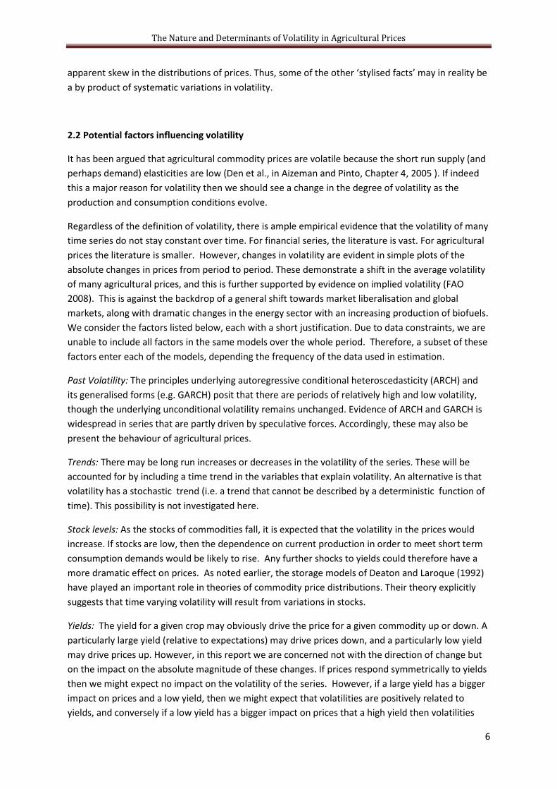
At the heart of this approach is the decomposition for the logged price 𝑦𝑡 at time t as in equation (3)
below.
𝑦𝑡 = 𝐿𝑒𝑣𝑒𝑙𝑡 + 𝑆𝑒𝑎𝑠𝑜𝑛𝑎𝑙𝑡 + 𝐶𝑦𝑐𝑙𝑒𝑡 3
The level component may either represent the mean of the series (if it is mean reverting) or may
trend upwards or downwards. The cyclical component, by definition, has a mean of zero and no
trend. However, the level components are driven by a set of shocks (𝑣𝑡), and the cyclical
components are driven by shocks (𝑒𝑡). Each of these are assumed to be random shocks, governed by
a time varying variances ℎ𝑣𝑡 and ℎ𝑒𝑡 respectively. Either one of these variances may be zero for a
given price, but both cannot be zero since this would imply that the series had no random variation.
For the level component, a variance of zero would imply a constant mean for the series, and
therefore all shocks are transitory. If the cyclical variance was zero, this would imply that all shocks
to prices were permanent.
The seasonal component is deterministic (does not depend on random shocks). Two different
methods of modelling the seasonality were explored. First ‘seasonal dummies’ were employed, whereby the series is allowed a seasonal component in each month. Alternatively, the seasonal
frequency approach from Harvey (1989 p.41) was employed. Here, there are potentially 11 seasonal
frequencies that can enter the model, the first of which is the ‘fundamental frequency’. The results
were largely invariant to the methods employed. However, the results that are presented in the
empirical section use the first seasonal frequency only.
The Level and Cyclical components have variance, which we label as follows: 𝑉𝑎𝑟 𝛥𝐿𝑒𝑣𝑒𝑙𝑡 : 𝑣𝑜𝑙𝑎𝑡𝑖𝑙𝑖𝑡𝑦 𝑖𝑛 𝑚𝑒𝑎𝑛
𝑉𝑎𝑟 𝐶𝑦𝑐𝑙𝑒 : 𝑣𝑜𝑙𝑎𝑡𝑖𝑙𝑖𝑡𝑦 𝑖𝑛 𝑐𝑦𝑐𝑙𝑒
Each of these are governed by an underlying volatility of a shock specific to each component, and
can (within the models outlined in the appendix) shown to be
𝑉𝑎𝑟 𝛥𝐿𝑒𝑣𝑒𝑙𝑡 = 𝐶𝑜𝑛𝑠𝑡𝑎𝑛𝑡𝐿 × ℎ𝑣,𝑡 𝑉𝑎𝑟 𝐶𝑦𝑐𝑙𝑒𝑡 = 𝐶𝑜𝑛𝑠𝑡𝑎𝑛𝑡𝐶 × ℎ𝑒 ,𝑡

The Nature and Determinants of Volatility in Agricultural Prices
9
Having made this decomposition, then we can make ℎ𝑣𝑡 and ℎ𝑒𝑡 depend on explanatory variables.
Within this report we consider the following explanatory variables for the volatilities, which we have
discussed earlier in Section 2:
i) a measure of the past realised volatility of the series ;
ii) realised oil price volatility;
iii) a measure of the average realised volatility in the other agricultural prices within the
data;
iv) stocks levels;
v) realised exchange rate volatility;
vi) realised interest rate volatility; and,
vii) a time trend;
In each case where we use the term ‘realised’ volatility, the measure will is the square of the
monthly change in the relevant series, as distinct from the ex ante measures ℎ𝑣𝑡 and
ℎ𝑒𝑡 respectively.
Using the approach above, we then produce:
i) measures in volatility (mean and cycle) for each of the agricultural price series through
time;
ii) tests for the persistence in the changes in volatility for these series;
iii) tests for the transmission of volatility across price series; and;
iv) tests for the transmission of volatility from oil prices, stocks etc to agricultural prices.
3.2 The panel approach
In order complement the approach above, use of annual data is also made. A panel approach is
used due to the relatively short series available (overlapping across all the variables) at the annual
frequency. The following approach is employed12
: 𝑙𝑛𝑉𝑖𝑡 = 𝛽0𝑖 + 𝛽1𝑖𝑡 + 𝜆𝑣𝑙𝑛𝑉𝑖 𝑡−1 + 𝜆′𝑧𝑖𝑡 + 𝑒𝑖𝑡 4
Where 𝑉𝑖𝑡 is a (realised) measure of volatility of the ith commodity at time t, 𝑧𝑖𝑡 is a vector of factors
that could explain volatility, and 𝑒𝑖𝑡 is assumed be normal with a variance that is potentially
different across the commodities, serially independent, but with a covariance across i
(commodities). We additionally estimate the model imposing 𝛽1𝑖 = 𝛽1 (a common time trend)
across the models. Thus this model is one with fixed effects (intercept and trend) across the
commodities13
.
12
The distribution of the volatilities was examined prior to estimation, and the logged volatilities had a
distribution that was reasonably consistent with being normal. Therefore, estimation was conducted in logged
form. 13
The issues of trends, stochastic trends and panel cointegration are not considered in this report. The
volatilities are unlikely to be I(1) processes, and certainly reject the hypothesis that they contain unit roots.

The Nature and Determinants of Volatility in Agricultural Prices
10
Within 𝑧𝑖𝑡 we consider the following:
i) realised oil price volatility;
ii) stocks;
iii) yields;
iv) realised exchange rate volatility; and,
v) realised export concentration (the Herfindhal index);
Where the price data is monthly, the realised annual volatility is defined herein as:
𝑉𝑖𝑡 = (𝛥12𝑗=1 ln 𝑝𝑖 .𝑗 .𝑡 )2
12 5
Where 𝑝𝑖.𝑗 .𝑡 is the price of the ith commodity in the jth
month of the 𝑡𝑡ℎ year. As noted earlier, there
are a number of other potential measures of annual volatility. However, the statistic above usefully
summarises intra year volatility into an annual measure. Alternative transformations (such as the
mean absolute deviation of price changes) are very similar when plotted against each other, and are
therefore likely to give similar results within a regression framework. The logged measure of
volatility (as defined in 5) is approximately normally distributed for the annual series used in this
report, which it attractive from an estimation point of view.
4 Estimation and interpretation
4.1 Estimation
The work in this study employs a Baeysian approach to estimation. The reason for using a Bayesian
framework is that it is a more robust method of estimation in the current context. The estimation of
the random parameter models can be performed using the Kalman Filter (Harvey 1989). The Kalman
Filter enables the likelihood of the models to be computed, and may be embedded within Monte
Carlo Markov Chain (MCMC) sampler that estimates the distributions of the parameters of interest.
A full description of the estimation procedures are beyond the scope of this report as while many of
the methods are now standard within Bayesian econometrics, a full description would run into many
pages. Good starting references include Chib and Greenberg (1995) and Koop (2003). A brief
coverage of the estimation procedures is given in the technical appendix (B2).
4.2 Interpretation of the parameter estimates and standard deviations
In interpreting the estimates produced in this report, readers may essentially adopt a classical
approach (the statistical approach with which most readers are more likely to be familiar). Strictly
speaking, the Bayesian approach requires some subtle differences in thinking. However, there are
theoretical results (see Train, 2003) establishing that using the mean of the posterior (the Bayesian
Stochastic trends could exist in the stocks, yield and export concentration data, and we recognise therefore
these could have an influence on the results.

The Nature and Determinants of Volatility in Agricultural Prices
11
estimate of a parameter) is equivalent to the ‘maximum likelihood’ estimate (one of the most
commonly used classical estimate), sharing the property of asymptotic efficiency. As the sample size
increases and the posterior distribution normalises, the Bayesian estimate is asymptotically
equivalent to the maximum likelihood estimator and the variance of the posterior identical to the
sampling variance of the maximum likelihood estimator (Train 2003). Therefore, we will continue to
talk in terms of ‘significance’ of parameters, even though strictly speaking p-values are not delivered
within the Bayesian methodology (and for this reason are not produced within the results section).
Broadly speaking, if the estimate is twice as large as its standard deviation then this is roughly
consistent with that estimate being statistically significant at the 5% level.
5 Empirical Results
5.1 Data
The data for this study were provided by FAO. A summary of the length and frequency of the data is
provided in Table 1. The models discussed in the previous section will be estimated using this data.
The first set of models outlined in section 3 will be run on the monthly series, and the panel
approach will be used for the annual data. The annual price volatilities were calculated from the
monthly data. There are 19 commodities listed in the tables.
Because some of the variables are recorded over a shorter period that others, the models will be run
using a subset of the data for longer periods and all of the variables for longer periods. Where stocks
are used in the models, at a monthly frequency, they were interpolated from the quarterly data, but
the models were estimated at the shorter frequency.14
5.2 Results
5.2.1 Monthly results.
We begin with the results for the monthly data run over the longest possible period for each
commodity. In the first instance exchange rates were not included, since these were available only
from 1973 onwards (see Table 1). The models using monthly data were then re-estimated including
exchange rates (over the shorter period). When running the models, we imposed positivity
restrictions on the coefficients of some of the explanatory variables. Without these restrictions, a
minority of commodities had perverse signs on some of the coefficients, though in nearly all cases
these were insignificant. The monthly results are presented in Tables 2 to 21. In each case the results
for the model with and without exchange rates are presented for each commodity. Importantly, the
time period over which the two sets of results are obtained differs for the case where exchange
rates are included, since exchange rates were only available from 1973 onwards. The difference in
the parameter values will therefore differ due to this as well as the inclusion of exchange rates.
Table 21 presents the monthly results for the three series for which stocks data are available.
14
Weekly prices also exist for a few commodities only. We did analyse this data, but the results were rather
inconclusive. Our analysis of this data are not included in this report but are available.

The Nature and Determinants of Volatility in Agricultural Prices
12
In Tables 2 through 24, the error variance refers to the square root estimate of the intercept for ℎ𝑒
as defined in Section 3. The Random intercept variance is the square root of intercept estimate of ℎ𝑣. The rest of the parameter estimates are the lambda parameters in equations b10 and b11 (in
Appendix B) where these are the coefficients of the variables listed in the first column of each table.
The last four coefficients in each table are: the intercept; estimates of the autoregressive
coefficients; and, the seasonal coefficient (the first fundamental frequency) .
The estimates within the table are the means and standard deviations of the posterior distributions
of the parameters. In each case the significance of a variable is signified by the estimate being in
bold italics indicating that the standard deviation is less than 1.64 of the absolute mean of the
posterior distribution. As noted in Section 4.2, this roughly corresponds to a variable being
significant at the 5% level (one tailed).
While the focus of our analysis is mainly on the determinants of the volatility of the series, it is worth
nothing that the autoregressive representation of order two is sufficient to capture the serial
correlation in the series. The first lag is significant for most of the commodities. In only a few cases
is the second order coefficient significant. However having said this, the majority of the series have
negative second order coefficients suggesting that the majority of the series contain cyclical
behaviour. The seasonal components of the series are insignificant for nearly all commodities.15
While the second order coefficient and seasonal components could be removed, an exploratory
analysis suggested that inclusion of these components had not substantive impact on the results.
Therefore, for consistency, these explanatory variables are included for all the series.
Table 23 summarises the results for the monthly data, from Tables 2 through 21. Each series has
two sets of results in tables 2 through 20. The first is where the model is run on the longest possible
period, excluding exchange rate volatility. The second is on the shorter series where exchange rate
volatility is included. Therefore, the two sets of results will differ because an additional variable is
included and they are run over different periods. The stocks data was available for only 3 of the
series (Wheat, Maize and Soyabean). Therefore, there is another table (21) which utilises the stocks
data. Again, this is run over a shorter period than for all the previous results, since the stocks data is
only available from the periods listed in Table 1. The rest of the column in in Table 1 is blacked out
for the other commodities for which stocks data is unavailable. A tick (√) in a given cell indicates that the variable listed in the column heading is significant in influencing the volatility of the series for
one of models in Tables 2 through 20. Two ticks in a cell indicate that the variable was significant for
both the models (i.e. with and without exchange rates).
Broadly, the results in Table 23 (and Tables 2 through 21) can be summarised as follows:
i) Nearly all the commodities have significant stochastic trends (as the variance in the
random intercept is significant). Pigmeat is the exception.
ii) Most of the commodities have cylcial components with the exception of palm oIl.
15
This finding was supported when the series were estimated with higher seasonal frequencies and seasonal
dummies.

The Nature and Determinants of Volatility in Agricultural Prices
13
iii) Past volatility is a significant predictor of current volatility for nearly all variables run
over both periods (with and without exchange rate volatility). We therefore
conclude that there is persistent volatility in commodity prices. That is, we would
expect to see periods of relatively high volatility in agricultural commodities and
periods of relatively low volatility.
iv) There is evidence that there is transmission of volatility across agricultural
commodities for nearly all commodities (except pigmeat). The aggregate past
volatility is a predictor of volatility in most commodities. This is indicative of a
situation where markets are experience common shocks that impact on many
markets rather than being isolated to one commodity or market.
v) Oil price volatility a significant predictor of volatility in agricultural commodities in
the majority series. With the growth of the biofuel sector, commodity prices and oil
prices may become more connected, so there is reason to believe that the role of oil
prices in determining volatility may even be stronger in the future.
vi) As with oil prices, exchange Rate volatility impacts on the volatility of commodity
prices for 10 out of the 19 series.
vii) Stock levels have a significant (downward) impact on the volatility for each of the
three series for which we have data on stocks. This is consistent with our
expectations that as stocks become lower, the markets become more volatile.
viii) A number of commodity prices have significant trends. However, these trends are
positive for some series and negative for others. Recent high levels of volatility
should not lead us to believe that agricultural markets are necessarily becoming
more volatile in the long run.
5.2.2 Annual results
The annual results were produced using the panel approach outlined in Section 3.2 and are
presented in Table 22. Four sets of results are presented within that table. First, results are produced
with and without the inclusion of stocks. This is because the stocks data was for a shorter period
than for the commodity price data. Next, we allowed for the trends in the panel regression to be
restricted to be the same across each of the commodities, and in another model they were allowed
to vary, giving four sets of results overall.
Where stocks are included, stocks are significant for the model in which the trend is restricted, but
becomes insignificant when the trends in volatility are allowed to vary for each of the commodities.
Notably, the estimated trends are generally negative, and the restriction of common trends across
the commodities seems reasonable. Thus, the results do suggest (as with the higher frequency data)
that as stocks rise the level of volatility in the prices decreases.
As with the higher frequency data, there is strong evidence that there is persistence in volatility. This
finding is robust to the specification of the model since lagged volatility is significant in all four
specifications. Yields also appear to be a significant determinant of volatility. In each of the four
specifications higher yields lead to larger volatility in the series. As argued in Section 2.3, there is no
clear case for expecting yields to have a positive or negative influence on volatility in the first
instance. Obviously, we would expect high yields to drive prices down, and low yields to drive prices

The Nature and Determinants of Volatility in Agricultural Prices
14
up. However, this does not imply the volatility of the series should go up or down. Our results
suggest that high yields have a tendency to drive prices downwards to a greater extent than low
yields tend to drive prices up. While we do not investigate this further here, it is also possible that
the response to yields is dependent on the level of stocks.
Finally, unlike the higher frequency data, there is only weak evidence that oil price volatility and
exchange rate volatility have an impact on the volatility of commodity prices.
6 Conclusions
Several important findings emerge from our empirical study. First, there is strong evidence that
there is persistent volatility in agricultural series. In nearly all of the series examined, there was
evidence that the variance of the series was a function of the past volatility of the series, and this
finding was robust to the choice of model and frequency of the data. Next, there was convincing
evidence that there was some degree of transmission of volatility across commodities in the monthly
data. Where stocks and yield data were available, these also appeared to be significant determinants
of the volatility of agricultural commodity prices.
There is also convincing evidence that many of the candidate variables have an impact on volatility.
In monthly series, oil price volatility had a positive impact on commodity price volatility. Thus, from
the evidence available, the recent coincidental high volatility in oil and commodity prices is
symptomatic of a connection between commodity price volatility and oil price volatility. As discussed
earlier. the link between oil prices and agricultural commodity prices is likely to arise through the
impact of energy prices on the costs of production, along with the alternative use of some crops for
biofuel production. Therefore, we would expect the link between oil price volatility and agricultural
prices to continue or strengthen as the biofuels sector grows. Likewise, exchange rate volatility was
found to influence the volatility of agricultural prices. Thus, perhaps unsurprisingly, if the global
economy is experiencing high levels of volatility these will also be reflected in agricultural prices.
Although, in this study we could not identify any significant link between export concentration (as
measured by the Herfindahl index) and oil price volatility.
Finally, the evidence produced in this report also suggested volatility of agricultural prices contained
trends that were independent of the variables used to explain volatility in this report. However, the
evidence is mixed with regard to the direction of these changes. In the monthly data, these trends
were positive for some commodities and negative for others. For the annual data, the evidence was
that the trends were, having accounted for oil price volatility and other factors, negative. Thus,
overall the results here do not suggest that there will be increasing volatility in agricultural markets
unless there is increasing volatility in the variables that are determining that volatility. On the other
hand, if factors such as oil prices continue to be volatile, then agricultural prices may continue to be
volatile or become increasingly volatile.
The Nature and Determinants of Volatility in Agricultural Prices
15
References
J Aizeman and B Pinto (2005) Managing Economic Volatility and Crisis, A practitioners Guide,
Cambridge University Press. New York. World Bank (2005).
Balcombe K. and Rapsomanikis G (2008). Bayesian Estimation and Selection of Non‐Linear Vector Error Correction Models: The Case of the Sugar‐Ethanol‐Oil Nexus in Brazil. American Journal of
Agricultural Economics, 90 (2) 658-668.
Chib C. and E. Greenberg, (1995). Understanding the Metropolis-Hastings Algorithm. The American
Statistician, November, 1995, 49. No 4.: 327-335
Deaton A and Laroque G. (1992) On the behaviour of Commodity Prices. Review of Economic
Studies, 59, 1-23.
Engle R.F. (1982). Autoregressive Conditional Heteroscedasticity of the Variance of United Kingdom
Inflation. Econometrica. 50,4 987-1006.
Engle R.F (1995) . ARCH, Selected Readings. Advanced Texts in Econometrics. Oxford University
Press.
FAO (2008), Food Outloook, Global Market Analysis. June,
http://www.fao.org/docrep/010/ai466e/ai466e00.HTM
Harvey A.C. (1989). Forecasting structural time series models and the Kalman filter. Cambridge
University Press. Cambridge.
Lex Oxley, Donald A. R., Colin J., Stuart Sayer (1994) Surveys in Econometrics. Wiley Blackwell.
Kenneth Train (2003). Discrete Choice Methods with Simulation. Cambridge University Press, 2003
Koop G. (2003) Bayesian Econometrics, Wiley, Sussex, England.

The Nature and Determinants of Volatility in Agricultural Prices
16
Appendix A: Tables
Table 1. Data Series Summary
Frequency Annual Annual Annnual Monthly Quarterly
Series Stocks Yeild Herfindel Price Stocks
Commodity
Wheat 1
1962-
2007
1962-
2007
1961-
2006
Jan 57-
Mar09 June:1977-Dec2008
Maize 2
1962-
2007
1962-
2007
1961-
2006
Jan 57-
Mar09 June1975:June2008
Rice, Milled 3
1962-
2007
1962-
2007
1961-
2006
Jan 57-
Mar09
Oilseed,
Soybean 4
1962-
2007
1962-
2007
1961-
2006
Jan 57-
Jan09 Dec1990:Dec:2008
Oil, Soybean 5
1962-
2007
1961-
2006
Jan 57-
Jan09
Oil, Rapeseed 6
1962-
2007
1962-
2007
1961-
2006
Jan70-
Jan09
Oil, Palm 7
1962-
2007
1962-
2007
1961-
2006
Jan60-
Jan09
Poultry, Meat,
Broiler 8
1962-
2007
1961-
2006
Feb80-
Nov08
Meat, Swine 9
1962-
2007
1961-
2006
Feb80-
Nov08
Meat, Beef
and Veal 10
1962-
2007
1961-
2006
Jan57-
Oct08
Dairy, Butter 11
1962-
2007
1961-
2006
Jan57-
Jan09
Dairy, Milk,
Nonfat Dry 12
1962-
2007
1961-
2006
Jan90-
Jan09
Dairy, Dry
Whole Milk
Powder 13
1962-
2007
1961-
2006
Jan90-
Jan09
Dairy, Cheese 14
1962-
2007
1961-
2006
Jan90-
Jan09
Cocoa 15
1962-
2007
1961-
2006
Jan57-
Nov08
Coffee, Green 16
1962-
2007
1962-
2007
1961-
2006
Jan57-
Nov08
Tea 17
1962-
2007
1961-
2006
Jan57-
Nov08
Sugar 18
1962-
2007
1962-
2007
1961-
2006
Jan57-
Nov08
Cotton 19
1962-
2007
1962-
2007
1961-
2006
Jan57-
Nov08
Other Data
Frequency
Monthly
Oil Prices
Jan 57-
Mar09
Exchange Rates
1973-2007
Interest Rates (US 6 month Treasury Bill)

The Nature and Determinants of Volatility in Agricultural Prices
17
Tables: Monthly Data
Table 2. Wheat (Monthly) Table 3. Maize (Monthly)
Parameter Mean Stdv Mean Stdv Parameter Mean Stdv Mean Stdv
Error Variance 0.02 0.007 0.029 0.01 Error Variance 0.035 0.009 0.04 0.015
Random intercept variance 0.037 0.005 0.035 0.011 Random intercept
variance
0.016 0.011 0.021 0.018
Lagged Own Volatility 0.268 0.046 0.097 0.042 Lagged Own Volatility 0.128 0.071 0.051 0.035
Lagged AggVolatility 0.24 0.095 0.351 0.092 Lagged AggVolatility 0.3 0.041 0.155 0.049
Oil Volatility 0.054 0.037 0.196 0.076 Oil Volatility 0.163 0.054 0.163 0.057
Trend 0.3 0.078 0.06 0.064 Trend 0.431 0.059 0.068 0.041
Ex Rate Volatility 0.043 0.03 Ex Rate Volatility 0.112 0.062
Mean Intercept 3.178 1.537 2.982 1.576 Mean Intercept 1.932 1.144 1.958 1.148
y(-1) 0.514 0.28 0.563 0.283 y(-1) 0.765 0.246 0.728 0.255
y(-2) -0.099 0.255 -0.111 0.269 y(-2) -0.145 0.242 -0.114 0.254
Seasonal 0.012 0.022 0.009 0.028 Seasonal 0.009 0.017 0.011 0.024
Table 4. Rice (Monthly) Table 5. Soyabean (Monthly)
Parameter Mean Stdv Mean Stdv Parameter Mean Stdv Mean Stdv
Error Variance 0.025 0.007 0.026 0.009 Error Variance 0.032 0.006 0.035 0.009
Random intercept variance 0.039 0.007 0.038 0.009 Random intercept
variance
0.03 0.008 0.035 0.01
Lagged Own Volatility 0.293 0.037 0.311 0.07 Lagged Own Volatility 0.199 0.032 0.232 0.073
Lagged AggVolatility 0.079 0.025 0.118 0.071 Lagged AggVolatility 0.369 0.105 0.189 0.055
Oil Volatility 0.095 0.037 0.301 0.071 Oil Volatility 0.033 0.03 0.086 0.081
Trend 0.064 0.043 0.053 0.056 Trend 0.1 0.062 -0.236 0.057
Ex Rate Volatility 0.078 0.055 Ex Rate Volatility 0.201 0.104
Mean Intercept 3.247 1.588 2.975 1.79 Mean Intercept 2.938 1.496 3.098 1.602
y(-1) 0.589 0.257 0.677 0.299 y(-1) 0.627 0.271 0.614 0.289
y(-2) -0.099 0.236 -0.144 0.277 y(-2) -0.129 0.255 -0.142 0.272
Seasonal -0.004 0.023 0.005 0.027 Seasonal 0.006 0.021 0.005 0.027
Table 6. Soya Oil (Monthly) Table 7. Rape (Monthly)
Parameter Mean Stdv Mean Stdv Parameter Mean Stdv Mean Stdv
Error Variance 0.02 0.01 0.012 0.008 Error Variance 0.018 0.011 0.018 0.011
Random intercept variance 0.05 0.007 0.057 0.005 Random intercept
variance
0.055 0.008 0.052 0.007
Lagged Own Volatility 0.226 0.033 0.134 0.069 Lagged Own Volatility 0.107 0.039 0.111 0.052
Lagged AggVolatility 0.169 0.047 0.139 0.068 Lagged AggVolatility 0.263 0.083 0.244 0.023
Oil Volatility 0.104 0.042 0.19 0.108 Oil Volatility 0.039 0.023 0.098 0.074
Trend -0.076 0.057 -0.338 0.104 Trend -0.296 0.075 -0.4 0.079
Ex Rate Volatility 0.358 0.113 Ex Rate Volatility 0.16 0.12
Mean Intercept 3.936 1.592 4.621 1.78 Mean Intercept 4.428 1.75 4.412 1.844
y(-1) 0.521 0.229 0.469 0.244 y(-1) 0.522 0.242 0.528 0.256
y(-2) -0.119 0.208 -0.168 0.223 y(-2) -0.183 0.226 -0.187 0.239
Seasonal -0.001 0.025 -0.009 0.031 Seasonal 0.003 0.028 0.002 0.03
Table 8. Palm (Monthly) Table 9. Poultry (Monthly)
Parameter Mean Stdv Mean Stdv Parameter Mean Stdv Mean Stdv
Error Variance 0.012 0.008 0.011 0.009 Error Variance 0.005 0.003 0.005 0.003
Random intercept variance 0.069 0.004 0.069 0.005 Random intercept
variance
0.02 0.002 0.02 0.002
Lagged Own Volatility 0.266 0.044 0.209 0.068 Lagged Own Volatility 0.217 0.038 0.095 0.069
Lagged AggVolatility 0.207 0.044 0.186 0.064 Lagged AggVolatility 0.115 0.034 0.037 0.025
Oil Volatility 0.164 0.06 0.154 0.066 Oil Volatility 0.031 0.015 0.037 0.018
Trend -0.212 0.065 -0.298 0.069 Trend -0.188 0.08 -0.149 0.111
Ex Rate Volatility 0.259 0.084 Ex Rate Volatility 0.13 0.048
Mean Intercept 4.616 1.553 4.67 1.541 Mean Intercept 2.863 1.975 2.799 1.91
y(-1) 0.433 0.228 0.437 0.225 y(-1) 0.475 0.421 0.484 0.409
y(-2) -0.172 0.2 -0.184 0.199 y(-2) -0.118 0.387 -0.113 0.387
Seasonal 0.017 0.032 0.016 0.033 Seasonal -0.012 0.022 -0.013 0.023

The Nature and Determinants of Volatility in Agricultural Prices
18
Table 10. Pigmeat (Monthly) Table 11. Beef (Monthly)
Parameter Mean Stdv Mean Stdv Parameter Mean Stdv Mean Stdv
Error Variance 0.097 0.002 0.098 0.002 Error Variance 0.019 0.009 0.021 0.008
Random intercept variance 0.004 0.003 0.004 0.003 Random intercept
variance
0.022 0.009 0.029 0.007
Lagged Own Volatility 0.124 0.068 0.087 0.029 Lagged Own Volatility 0.197 0.049 0.259 0.098
Lagged AggVolatility 0.059 0.036 0.062 0.029 Lagged AggVolatility 0.055 0.041 0.123 0.034
Oil Volatility 0.094 0.045 0.302 0.046 Oil Volatility 0.028 0.023 0.035 0.026
Trend -0.141 0.096 -0.154 0.047 Trend 0.273 0.107 -0.176 0.058
Ex Rate Volatility 0.06 0.036 Ex Rate Volatility 0.050 0.041
Mean Intercept 0.887 0.541 0.895 0.54 Mean Intercept 3.261 1.949 3.166 1.656
y(-1) 0.868 0.189 0.862 0.18 y(-1) 0.534 0.365 0.587 0.322
y(-2) -0.083 0.195 -0.078 0.186 y(-2) -0.150 0.346 -0.184 0.300
Seasonal 0.025 0.027 0.025 0.026 Seasonal -0.003 0.024 0.004 0.024
Table 12. Butter (Monthly) Table 13. SMP (Monthly)
Parameter Mean Stdv Mean Stdv Parameter Mean Stdv Mean Stdv
Error Variance 0.056 0.009 0.064 0.01 Error Variance 0.037 0.015 0.033 0.009
Random intercept variance 0.059 0.011 0.058 0.012 Random intercept
variance
0.05 0.012 0.038 0.009
Lagged Own Volatility 0.397 0.107 0.326 0.108 Lagged Own Volatility 0.518 0.146 0.529 0.098
Lagged AggVolatility 0.126 0.053 0.062 0.048 Lagged AggVolatility 0.234 0.092 0.12 0.07
Oil Volatility 0.181 0.104 0.155 0.062 Oil Volatility 0.377 0.129 0.283 0.097
Trend 0.032 0.068 -0.288 0.097 Trend -0.703 0.273 -0.477 0.147
Ex Rate Volatility 0.16 0.077 Ex Rate Volatility 0.216 0.061
Mean Intercept 4.601 1.39 4.466 1.517 Mean Intercept 2.232 2.532 2.256 2.676
y(-1) 0.057 0.218 0.056 0.236 y(-1) 0.62 0.389 0.609 0.414
y(-2) 0.052 0.198 0.038 0.22 y(-2) 0.077 0.36 0.085 0.386
Seasonal 0.01 0.029 0.003 0.035 Seasonal -0.001 0.029 0 0.031
Table 14. WMP (Monthly) Table 15. Cheese (Monthly)
Parameter Mean Stdv Mean Stdv Parameter Mean Stdv Mean Stdv
Error Variance 0.013 0.007 0.013 0.008 Error Variance 0.014 0.006 0.016 0.007
Random intercept variance 0.033 0.005 0.035 0.006 Random intercept
variance
0.027 0.005 0.026 0.006
Lagged Own Volatility 0.507 0.1 0.46 0.174 Lagged Own Volatility 0.351 0.062 0.478 0.134
Lagged AggVolatility 0.077 0.037 0.156 0.084 Lagged AggVolatility 0.163 0.052 0.068 0.045
Oil Volatility 0.18 0.067 0.076 0.032 Oil Volatility 0.18 0.026 0.226 0.037
Trend -0.148 0.097 -0.084 0.145 Trend -0.044 0.058 -0.068 0.105
Ex Rate Volatility 0.337 0.213 Ex Rate Volatility 0.125 0.075
Mean Intercept 2.682 3.261 2.883 3.289 Mean Intercept 3.171 3.661 3.103 3.746
y(-1) 0.588 0.45 0.566 0.444 y(-1) 0.433 0.475 0.448 0.495
y(-2) 0.051 0.401 0.047 0.394 y(-2) 0.165 0.434 0.159 0.449
Seasonal 0.002 0.034 0.003 0.034 Seasonal 0.002 0.031 0.002 0.03
Table 16. Cocoa (Monthly) Table 17. Coffee (Monthly)
Parameter Mean Stdv Mean Stdv Parameter Mean Stdv Mean Stdv
Error Variance 0.031 0.013 0.03 0.014 Error Variance 0.025 0.007 0.033 0.012
Random intercept variance 0.041 0.012 0.046 0.014 Random intercept
variance
0.051 0.007 0.07 0.01
Lagged Own Volatility 0.2 0.109 0.206 0.099 Lagged Own Volatility 0.496 0.1 0.492 0.077
Lagged AggVolatility 0.088 0.048 0.037 0.032 Lagged AggVolatility 0.181 0.066 0.038 0.029
Oil Volatility 0.311 0.22 0.089 0.06 Oil Volatility 0.106 0.061 0.108 0.056
Trend 0.082 0.14 -0.195 0.08 Trend 0.858 0.109 0.102 0.063
Ex Rate Volatility 0.083 0.059 Ex Rate Volatility 0.076 0.057
Mean Intercept 4.633 2.945 4.499 1.984 Mean Intercept 2.025 1.645 2.487 1.318
y(-1) 0.436 0.36 0.527 0.254 y(-1) 0.468 0.266 0.393 0.262
y(-2) -0.044 0.346 -0.116 0.242 y(-2) 0.088 0.235 0.065 0.228
Seasonal -0.002 0.04 0 0.03 Seasonal 0.011 0.021 0.027 0.036

The Nature and Determinants of Volatility in Agricultural Prices
19
Table 18. Tea (Monthly) Table 19. Sugar (Monthly)
Parameter Mean Stdv Mean Stdv Parameter Mean Stdv Mean Stdv
Error Variance 0.046 0.006 0.037 0.008 Error Variance 0.056 0.014 0.047 0.02
Random intercept variance 0.044 0.008 0.055 0.008 Random intercept
variance
0.06 0.015 0.064 0.019
Lagged Own Volatility 0.375 0.06 0.385 0.1 Lagged Own Volatility 0.251 0.043 0.253 0.08
Lagged AggVolatility 0.085 0.045 0.161 0.066 Lagged AggVolatility 0.099 0.048 0.088 0.061
Oil Volatility 0.035 0.028 0.046 0.036 Oil Volatility 0.102 0.067 0.141 0.072
Trend -0.098 0.031 0.03 0.08 Trend -0.234 0.047 -0.38 0.081
Ex Rate Volatility 0.028 0.025 Ex Rate Volatility 0.306 0.111
Mean Intercept 3.935 1.292 3.982 1.648 Mean Intercept 1.147 0.513 1.22 0.654
y(-1) 0.568 0.22 0.503 0.267 y(-1) 0.629 0.183 0.584 0.219
y(-2) -0.277 0.206 -0.222 0.243 y(-2) -0.093 0.172 -0.078 0.205
Seasonal 0.015 0.027 0.022 0.035 Seasonal 0.013 0.029 0.006 0.035
Table 20. Cotton (Monthly)
Parameter Mean Stdv Mean Stdv
Error Variance 0.017 0.007 0.039 0.004
Random intercept variance 0.023 0.008 0.004 0.006
Lagged Own Volatility 0.253 0.12 0.181 0.043
Lagged AggVolatility 0.203 0.085 0.119 0.097
Oil Volatility 0.133 0.048 0.219 0.11
Trend 0.364 0.134 0.004 0.047
Ex Rate Volatility 0.071 0.037
Mean Intercept 1.523 1.205 0.741 0.606
y(-1) 0.813 0.288 1.156 0.254
y(-2) -0.198 0.272 -0.338 0.254
Seasonal 0.005 0.017 0.007 0.016
Table 21. (Monthly with Stocks)
Wheat Maize Soyabean
Parameter Mean Stdv Mean Stdv Mean Stdv
Error variance 0.019 0.011 0.04 0.01 0.016 0.008
Random intercept
variance 0.037 0.01 0.017 0.013 0.043 0.006
Lagged Own Volatility 0.1 0.071 0.064 0.039 0.076 0.066
Lagged Aggregate
Volatility0.02 0.017 0.109 0.07 0.101 0.054
Stocks -0.11 0.031 -0.128 0.073 -0.324 0.111
Trend 0.338 0.164 0.441 0.164 0.045 0.035
Exchange Rate Vol 0.238 0.124 0.34 0.124 0.059 0.049
Oil Price Vol 0.1 0.071 0.064 0.039 0.076 0.066
mean intercept 3.274 1.773 1.538 1.569 4.009 1.86
y(-1) 0.459 0.293 0.712 0.365 0.488 0.287
y(-2) -0.059 0.278 -0.02 0.366 -0.109 0.272
Seasonal -0.014 0.03 0.015 0.031 -0.006 0.029

The Nature and Determinants of Volatility in Agricultural Prices
20
Table 22. Panel Results
Stocks Included (9 Commodities) Stocks Not Included
(9 Commodities) (11 Commodities)
Estimate Stdv Estimate Stdv
Lagged price volatility 0.392 0.064 0.392 0.063
Stock levels -0.103 0.055
Export concentration -0.07 0.104 -0.008 0.099
Yeilds 0.414 0.233 0.487 0.219
Exchange rate 0.301 0.283 0.297 0.278
Oil Price Volatility 0.081 0.054 0.077 0.055
Intercepts
Wheat -0.834 0.064 -0.833 0.07
Maize -0.764 0.057 -0.763 0.061
Rice -0.85 0.091 -0.852 0.093
Soybeans -0.793 0.074 -0.794 0.08
Rapeseed -0.647 0.076 -0.649 0.086
Palm Oil -0.454 0.076 -0.457 0.086
Cocoa -0.549 0.076
Coffee -0.363 0.102 -0.362 0.108
Tea -0.458 0.095
Sugar -0.148 0.068 -0.148 0.07
Cotton -0.845 0.078 -0.845 0.08
Pooled Trend -0.083 0.042 -0.116 0.041
Trends varying across
Volatility
Lagged price volatility 0.357 0.066 0.344 0.065
Stock levels -0.075 0.054
Export concentration -0.01 0.136 0.042 0.125
Yeilds 0.521 0.366 0.672 0.337
Exchange rate 0.298 0.28 0.296 0.276
Oil Price Volatility 0.074 0.052 0.07 0.052
Intercepts
Wheat -0.833 0.067 -0.833 0.072
Maize -0.765 0.06 -0.763 0.062
Rice -0.853 0.093 -0.854 0.094
Soybeans -0.794 0.075 -0.793 0.081
Rapeseed -0.647 0.076 -0.647 0.082
Palm Oil -0.455 0.077 -0.455 0.083
Cocoa -0.548 0.075
Coffee -0.361 0.101 -0.364 0.107
Tea -0.458 0.093
Sugar -0.148 0.068 -0.148 0.07
Cotton -0.843 0.08 -0.844 0.084
Trends
Wheat -0.094 0.107 -0.122 0.105
Maize -0.122 0.093 -0.165 0.089
Rice -0.14 0.117 -0.195 0.111
Soybeans -0.129 0.112 -0.192 0.102
Rapeseed -0.231 0.123 -0.313 0.114
Palm Oil -0.22 0.14 -0.324 0.125
Cocoa -0.232 0.091
Coffee 0.027 0.115 0.012 0.117
Tea -0.081 0.117
Sugar -0.164 0.076 -0.196 0.075
Cotton -0.098 0.103 -0.146 0.101

The Nature and Determinants of Volatility in Agricultural Prices
21
Table 23
Summary
of
Monthly
Data
Summary
of
Monthly
Data
Error
Variance
Random
Intercept
Variance
Past Own
Volil ity
Lag
Aggregate
Volatity
Oil
Volatil ity Trend Exrate Vol Stocks
2 Wheat √√ √√ √√ √√ √(+)√(+) √
3 Maize √√ √ √ √√ √√ √(+)√(+) √ √
4 Rice √√ √√ √√ √√ √√
5 Soyabean √√ √√ √√ √√ √(‐) √ √
6 Soya Oil √ √√ √√ √√ √√ √(‐) √
7 Rape √√ √ √√ √√ √ √(‐)√(‐)
8 Palm √√ √√ √√ √√ √(‐)√(‐) √
9 Poultry √√ √√ √ √ √ √( ‐) √
10 Pigmeat √√ √√ √√ √( ‐) √
11 Beef √√ √√ √√ √ √(+)√(‐)
12 Butter √√ √√ √√ √ √√ √( ‐) √
13 SMP √√ √√ √√ √√ √√ √(‐)√(‐) √
14 WMP √ √√ √√ √√ √√
15 Cheese √√ √√ √√ √ √√ √(‐) √
16 Cocoa √√ √√ √√ √√
17 Coffee √√ √√ √√ √ √√
18 Tea √√ √√ √√ √√ √(‐)
19 Sugar √√ √√ √√ √ √ √(‐)√(‐)
20 Cotton √√ √ √√ √ √√ √(+) √

The Nature and Determinants of Volatility in Agricultural Prices
22
Appendix B: Technical Appendix
B1 Random Parameter Models with Time Varying Volatility
For a given price series 𝑦𝑡 (or logged series which will be used throughout this report) where
t=1.....T, it is proposed that the following autoregressive model with a random walk intercept is
used: 𝜃 𝐿 𝑦𝑡 = 𝛼𝑡 + 𝛿 ′𝑑𝑡 + 𝑒𝑡 (𝑏1)
Where 𝜃 𝐿 = 𝜃𝑖𝐿𝑖 𝑘𝑖=0 (a lag operator of finite length) and: 𝛼𝑡 = 𝛼𝑡−1 + 𝑣𝑡 𝑏2 where 𝑑𝑡 is a vector of deterministic variables
16 that are able to capture the seasonality and 𝑒𝑡 and 𝑣𝑡 are assumed to be independently normally distributed. The series can then be decomposed into
its components: 𝑦𝑡 = 𝐿𝑒𝑣𝑒𝑙𝑡 + 𝑆𝑒𝑎𝑠𝑜𝑛𝑎𝑙𝑡 + 𝐶𝑦𝑐𝑙𝑒𝑡 𝑏3 𝐿𝑒𝑣𝑒𝑙: 𝜇𝑡 = 𝜃 𝐿 −1 1− 𝐿 −1𝑣𝑡 (𝑏4) 𝑆𝑒𝑎𝑠𝑜𝑛𝑎𝑙 ∶ 𝑠𝑡 = 𝛿 ′𝜃 𝐿 −1𝑑𝑡 (𝑏5) 𝐶𝑦𝑐𝑙𝑒 ∶ 𝑦𝑡 − 𝜇𝑡 − 𝑠𝑡 = 𝜃 𝐿 −1𝑒𝑡 𝑏6 Therefore, this allows the separate analysis of the non-stationary component 𝜇𝑡 and the stationary
component 𝑦𝑡 − 𝜇𝑡 . The overall volatility of the series are governed by the two variances. ℎ = ℎ𝑣 ,ℎ𝑒 along with the autoregressive parameters. The observed volatility are produced by the
errors 𝑒𝑡 ,𝑣𝑡 (which are assumed to be iid normal).
The inverted lag operator has the representation: 𝜃(𝐿)⁻¹ = 𝛾𝑖𝐿𝑖 (𝑏7)
∞𝑖=0
In the absence of stochastic volatility, the volatility in each of the series is governed by:
𝑉𝑎𝑟 𝛥𝜇𝑡 = 𝛾𝑗2∞
𝑗=0
ℎ𝑣 (𝑏8)
𝑉𝑎𝑟 𝑦𝑡 − 𝜇𝑡 − 𝑠𝑡 = 𝛾𝑗2∞𝑗=0
ℎ𝑒 𝑏9 16
In this case we examined both standard seasonal dummies along with the seasonal effects variables in
Harvey (1989, p.41). In virtually variables we found little evidence of seasonality. For the results presented in
this report, we continue to include the first fundamental frequency. However, in nearly all cases this was not
significant. We continue to include it for consistency across models. However, removing the seasonal dummies
would make little difference to the results presented here.

The Nature and Determinants of Volatility in Agricultural Prices
23
For a stationary series ℎ𝑣 = 0, in which case only 𝑉𝑎𝑟 𝑦𝑡 − 𝜇 is of interest. The proposed
framework is able to cope with stationary or non-stationary series, since there is no requirement
that ℎ𝑣 > 0 within the model. For the purposes of this study, the distinction between two volatilities
will be made as follows:
𝑉𝑎𝑟(𝛥𝜇𝑡): 𝑣𝑜𝑙𝑎𝑡𝑖𝑙𝑖𝑡𝑦 𝑖𝑛 𝑚𝑒𝑎𝑛
𝑉𝑎𝑟 𝑦𝑡 − 𝜇𝑡 − 𝑠𝑡 : 𝑣𝑜𝑙𝑎𝑡𝑖𝑙𝑖𝑡𝑦 𝑖𝑛 𝑐𝑦𝑐𝑙𝑒
The model can be extended by conditioning the variances on a set of explanatory variables in the
following way: 𝑙𝑛ℎ𝑣,𝑡 = ln ℎ𝑣 + 𝜆𝑣 ’ 𝑧𝑡 (𝑏10) 𝑙𝑛ℎ𝑒 ,𝑡 = ln ℎ𝑒 + 𝜆𝑒 ’ 𝑧𝑡 (𝑏11)
Where 𝑧𝑡 is a vector of variables as outlined in the main text in Section 3.1.
The two measures of volatility at a particular time then become: 𝑉𝑎𝑟 𝛥𝜇𝑡 = 𝛾𝑗2∞𝑗=0
ℎ𝑣,𝑡 𝑏12 𝑉𝑎𝑟 𝑦𝑡 − 𝜇𝑡 − 𝑠𝑡 = 𝛾𝑗2∞
𝑗=0
ℎ𝑒 ,𝑡 (𝑏13)
(where these can be aggregated to overall measure of volatility).
Restrictions and Identification
In the framework outlined above, equations b12 and b13 imply that the underlying volatility is
governed by : ℎ𝑣,𝑡 = ℎ𝑣 exp 𝜆𝑣 ’ 𝑧𝑡 (𝑏14)
ℎ𝑒 ,𝑡 = ℎ𝑒 exp 𝜆𝑒 ’ 𝑧𝑡 (𝑏15)
If 𝜆𝑣 or 𝜆𝑒 are equal to zero then the volatility in the long or short run component are constants.
However, in the situation where ℎ𝑣 or ℎ𝑒 are zero then the associated parameters 𝜆𝑣 𝑜𝑟 𝜆𝑒 become
unidentified. This does not in itself preclude estimation within in a Bayesian framework. However,
unless the posterior densities of ℎ𝑣 and ℎ𝑒 are both heavily concentrated away from zero, then the
standard error of the lambda coefficients will be very large. If a series can be modelled in a way
where the variance could be attributed either to stationary or non-stationary shocks, then the
associated standard deviation in the estimates of the lambda coefficients will be large, and
determining whether the shocks in the variable in question are significant will be very difficult. In
this work we avoid this problem by assuming 𝜆𝑣 = 𝜆𝑒 = 𝜆. This implies that the long run and short
run variances are proportional, but these variances can vary across in t. Since the values of ℎ𝑣 and ℎ𝑒

The Nature and Determinants of Volatility in Agricultural Prices
24
will not be close to zero simultaneously (since the all the series have variation) the standard errors in
the lambda coefficients will be smaller. This is obviously at a cost. If the shocks to volatility ( 𝑧𝑡 ) impacted differently on the long and short run components, then clearly there would be bias in the
results. However, arguably, it is reasonable to assume that shocks in volatility are likely to co-vary
across both the permanent and transitory components (should they both exist). Thus, while this
assumption is essentially required for identification, it is highly plausible from an economic point of
view.
B2 Estimation
Denoting the parameters that are to be estimated as Ω, the data to be explained as Y and the explanatory data as X, the likelihood function can be viewed as the probability density of Y
conditional on X and Ω. Therefore, the likelihood function can be denoted as𝑓(𝑌|Ω, X) . For prior
distributions on Ω, 𝑓(Ω), the posterior distribution is denoted as 𝑓(Ω|Y, X) and obeys: 𝑓 Ω Y, X ∝ 𝑓 𝑌 Ω, X 𝑓 Ω (𝑏16)
Where ∝ denotes proportionality. For the random parameter models, the parameters of interest
are: Ω∗ = 𝜃𝑗 ,𝜆𝑣 ,𝜆𝑒 ,ℎ𝑣 ,ℎ𝑒 (𝑏17)
Normal priors are adopted for the parameters 𝜃𝑗 , 𝜆𝑣 , 𝜆𝑒 where the mean is zero, with a large
variance so as to reflect diffuse prior knowledge.17
For the parameters ℎ𝑣 𝑎𝑛𝑑 ℎ𝑒 inverse gamma
priors can be used, as is standard in Bayesian analysis.
For any values of Ω = (𝜆𝑣 ,𝜆𝑒 ,ℎ𝑣 ,ℎ𝑒) the Kalman Filter can produce optimal estimates of 𝜃𝑗 , and
standard errors for these parameters, along with the value of the likelihood function. Thus, in effect 𝜃𝑗 are ignored in the estimation of since they are viewed as latent variables that are generated
for any given values of but are not required for the likelihood function. Estimation of the posterior
distributions are then obtained using a random walk Metropolis-Hastings algorithm (see Koop, 2003,
p97) to simulate the posterior distribution. The estimates of (Ω ) that are then produced are the
mean of the simulated parameters and the standard deviations for the simulated values can likewise
be obtained. The estimates for 𝜃𝑗 along with the standard errors are then obtained using the
values Ω within the Kalman Filter18
.
For the Panel Data a Bayesian approach to estimation is also used. In this case we use Gibbs
Sampling 19
. The parameters are simply, Ω = 𝛽𝑜𝑖 , 𝛽1𝑖 , 𝜆𝑣 ,𝜆,𝛴 (𝑏18)
Where 𝛴 is the variance covariance matrix associated with the errors in equation (4) within the main
text.
17
Note that the priors for the autoregressive coefficients are set within the Kalman Filter. 18
Note that these point estimates are therefore conditional on the plug in estimates and strictly speaking do
not reflect the mean and variance of these parameters from a Bayesian perspective. 19
A good coverage of Gibbs Sampling is given in many textbooks. The estimation procedure of this panel can
be viewed as a seemingly unrelated regression with cross equation restrictions. The details of how to estimate
this model are in Koop (2003) Chapter 6.