Embed Size (px)
Citation preview
The motion of point particles in curved spacetime
Eric Poisson, Adam Pound, and Ian VegaDepartment of Physics, University of Guelph, Guelph, Ontario, Canada N1G 2W1
Major update of Living Reviews article, with final revisions (September 25, 2011)
Abstract
This review is concerned with the motion of a point scalar charge, a point electric charge, and apoint mass in a specified background spacetime. In each of the three cases the particle produces a fieldthat behaves as outgoing radiation in the wave zone, and therefore removes energy from the particle.In the near zone the field acts on the particle and gives rise to a self-force that prevents the particlefrom moving on a geodesic of the background spacetime. The self-force contains both conservative anddissipative terms, and the latter are responsible for the radiation reaction. The work done by the self-forcematches the energy radiated away by the particle.
The field’s action on the particle is difficult to calculate because of its singular nature: the fielddiverges at the position of the particle. But it is possible to isolate the field’s singular part and show thatit exerts no force on the particle — its only effect is to contribute to the particle’s inertia. What remainsafter subtraction is a regular field that is fully responsible for the self-force. Because this field satisfiesa homogeneous wave equation, it can be thought of as a free field that interacts with the particle; it isthis interaction that gives rise to the self-force.
The mathematical tools required to derive the equations of motion of a point scalar charge, a pointelectric charge, and a point mass in a specified background spacetime are developed here from scratch.The review begins with a discussion of the basic theory of bitensors (part I). It then applies the theoryto the construction of convenient coordinate systems to chart a neighbourhood of the particle’s word line(part II). It continues with a thorough discussion of Green’s functions in curved spacetime (part III). Thereview presents a detailed derivation of each of the three equations of motion (part IV). Because the notionof a point mass is problematic in general relativity, the review concludes (part V) with an alternativederivation of the equations of motion that applies to a small body of arbitrary internal structure.
Contents
1 Introduction and summary 51.1 Invitation . . . . . . . . . . . . . . . . . . . . . . . . . . . . . . . . . . . . . . . . . . . . . . . 51.2 Radiation reaction in flat spacetime . . . . . . . . . . . . . . . . . . . . . . . . . . . . . . . . 51.3 Green’s functions in flat spacetime . . . . . . . . . . . . . . . . . . . . . . . . . . . . . . . . . 71.4 Green’s functions in curved spacetime . . . . . . . . . . . . . . . . . . . . . . . . . . . . . . . 81.5 World line and retarded coordinates . . . . . . . . . . . . . . . . . . . . . . . . . . . . . . . . 101.6 Retarded, singular, and regular electromagnetic fields of a point electric charge . . . . . . . . 121.7 Motion of an electric charge in curved spacetime . . . . . . . . . . . . . . . . . . . . . . . . . 131.8 Motion of a scalar charge in curved spacetime . . . . . . . . . . . . . . . . . . . . . . . . . . . 141.9 Motion of a point mass, or a small body, in a background spacetime . . . . . . . . . . . . . . 151.10 Case study: static electric charge in Schwarzschild spacetime . . . . . . . . . . . . . . . . . . 171.11 Organization of this review . . . . . . . . . . . . . . . . . . . . . . . . . . . . . . . . . . . . . 191.12 Changes relative to the 2004 edition . . . . . . . . . . . . . . . . . . . . . . . . . . . . . . . . 20
2 Computing the self-force: a 2010 literature survey 212.1 Early work: DeWitt and DeWitt; Smith and Will . . . . . . . . . . . . . . . . . . . . . . . . . 212.2 Mode-sum method . . . . . . . . . . . . . . . . . . . . . . . . . . . . . . . . . . . . . . . . . . 222.3 Effective-source method . . . . . . . . . . . . . . . . . . . . . . . . . . . . . . . . . . . . . . . 272.4 Quasilocal approach with “matched expansions” . . . . . . . . . . . . . . . . . . . . . . . . . 292.5 Adiabatic approximations . . . . . . . . . . . . . . . . . . . . . . . . . . . . . . . . . . . . . . 302.6 Physical consequences of the self-force . . . . . . . . . . . . . . . . . . . . . . . . . . . . . . . 31
arX
iv:1
102.
0529
v3 [
gr-q
c] 2
6 Se
p 20
11
Contents 2
I General theory of bitensors 34
3 Synge’s world function 343.1 Definition . . . . . . . . . . . . . . . . . . . . . . . . . . . . . . . . . . . . . . . . . . . . . . . 343.2 Differentiation of the world function . . . . . . . . . . . . . . . . . . . . . . . . . . . . . . . . 353.3 Evaluation of first derivatives . . . . . . . . . . . . . . . . . . . . . . . . . . . . . . . . . . . . 353.4 Congruence of geodesics emanating from x′ . . . . . . . . . . . . . . . . . . . . . . . . . . . . 36
4 Coincidence limits 374.1 Computation of coincidence limits . . . . . . . . . . . . . . . . . . . . . . . . . . . . . . . . . 374.2 Derivation of Synge’s rule . . . . . . . . . . . . . . . . . . . . . . . . . . . . . . . . . . . . . . 38
5 Parallel propagator 395.1 Tetrad on β . . . . . . . . . . . . . . . . . . . . . . . . . . . . . . . . . . . . . . . . . . . . . . 395.2 Definition and properties of the parallel propagator . . . . . . . . . . . . . . . . . . . . . . . . 395.3 Coincidence limits . . . . . . . . . . . . . . . . . . . . . . . . . . . . . . . . . . . . . . . . . . 40
6 Expansion of bitensors near coincidence 406.1 General method . . . . . . . . . . . . . . . . . . . . . . . . . . . . . . . . . . . . . . . . . . . . 406.2 Special cases . . . . . . . . . . . . . . . . . . . . . . . . . . . . . . . . . . . . . . . . . . . . . 416.3 Expansion of tensors . . . . . . . . . . . . . . . . . . . . . . . . . . . . . . . . . . . . . . . . . 42
7 van Vleck determinant 427.1 Definition and properties . . . . . . . . . . . . . . . . . . . . . . . . . . . . . . . . . . . . . . . 427.2 Derivations . . . . . . . . . . . . . . . . . . . . . . . . . . . . . . . . . . . . . . . . . . . . . . 43
II Coordinate systems 45
8 Riemann normal coordinates 458.1 Definition and coordinate transformation . . . . . . . . . . . . . . . . . . . . . . . . . . . . . 458.2 Metric near x′ . . . . . . . . . . . . . . . . . . . . . . . . . . . . . . . . . . . . . . . . . . . . . 45
9 Fermi normal coordinates 469.1 Fermi-Walker transport . . . . . . . . . . . . . . . . . . . . . . . . . . . . . . . . . . . . . . . 469.2 Tetrad and dual tetrad on γ . . . . . . . . . . . . . . . . . . . . . . . . . . . . . . . . . . . . . 479.3 Fermi normal coordinates . . . . . . . . . . . . . . . . . . . . . . . . . . . . . . . . . . . . . . 479.4 Coordinate displacements near γ . . . . . . . . . . . . . . . . . . . . . . . . . . . . . . . . . . 479.5 Metric near γ . . . . . . . . . . . . . . . . . . . . . . . . . . . . . . . . . . . . . . . . . . . . . 489.6 Thorne-Hartle-Zhang coordinates . . . . . . . . . . . . . . . . . . . . . . . . . . . . . . . . . . 49
10 Retarded coordinates 5010.1 Geometrical elements . . . . . . . . . . . . . . . . . . . . . . . . . . . . . . . . . . . . . . . . . 5010.2 Definition of the retarded coordinates . . . . . . . . . . . . . . . . . . . . . . . . . . . . . . . 5110.3 The scalar field r(x) and the vector field kα(x) . . . . . . . . . . . . . . . . . . . . . . . . . . 5110.4 Frame components of tensor fields on the world line . . . . . . . . . . . . . . . . . . . . . . . 5310.5 Coordinate displacements near γ . . . . . . . . . . . . . . . . . . . . . . . . . . . . . . . . . . 5410.6 Metric near γ . . . . . . . . . . . . . . . . . . . . . . . . . . . . . . . . . . . . . . . . . . . . . 5410.7 Transformation to angular coordinates . . . . . . . . . . . . . . . . . . . . . . . . . . . . . . . 5510.8 Specialization to aµ = 0 = Rµν . . . . . . . . . . . . . . . . . . . . . . . . . . . . . . . . . . . 56
Contents 3
11 Transformation between Fermi and retarded coordinates; advanced point 5711.1 From retarded to Fermi coordinates . . . . . . . . . . . . . . . . . . . . . . . . . . . . . . . . 5811.2 From Fermi to retarded coordinates . . . . . . . . . . . . . . . . . . . . . . . . . . . . . . . . 6011.3 Transformation of the tetrads at x . . . . . . . . . . . . . . . . . . . . . . . . . . . . . . . . . 6111.4 Advanced point . . . . . . . . . . . . . . . . . . . . . . . . . . . . . . . . . . . . . . . . . . . . 63
III Green’s functions 64
12 Scalar Green’s functions in flat spacetime 6412.1 Green’s equation for a massive scalar field . . . . . . . . . . . . . . . . . . . . . . . . . . . . . 6412.2 Integration over the source . . . . . . . . . . . . . . . . . . . . . . . . . . . . . . . . . . . . . 6412.3 Singular part of g(σ) . . . . . . . . . . . . . . . . . . . . . . . . . . . . . . . . . . . . . . . . . 6512.4 Smooth part of g(σ) . . . . . . . . . . . . . . . . . . . . . . . . . . . . . . . . . . . . . . . . . 6612.5 Advanced distributional methods . . . . . . . . . . . . . . . . . . . . . . . . . . . . . . . . . . 6612.6 Alternative computation of the Green’s functions . . . . . . . . . . . . . . . . . . . . . . . . . 68
13 Distributions in curved spacetime 6913.1 Invariant Dirac distribution . . . . . . . . . . . . . . . . . . . . . . . . . . . . . . . . . . . . . 6913.2 Light-cone distributions . . . . . . . . . . . . . . . . . . . . . . . . . . . . . . . . . . . . . . . 69
14 Scalar Green’s functions in curved spacetime 7014.1 Green’s equation for a massless scalar field in curved spacetime . . . . . . . . . . . . . . . . . 7014.2 Hadamard construction of the Green’s functions . . . . . . . . . . . . . . . . . . . . . . . . . 7114.3 Reciprocity . . . . . . . . . . . . . . . . . . . . . . . . . . . . . . . . . . . . . . . . . . . . . . 7214.4 Kirchhoff representation . . . . . . . . . . . . . . . . . . . . . . . . . . . . . . . . . . . . . . . 7314.5 Singular and regular Green’s functions . . . . . . . . . . . . . . . . . . . . . . . . . . . . . . . 7414.6 Example: Cosmological Green’s functions . . . . . . . . . . . . . . . . . . . . . . . . . . . . . 76
15 Electromagnetic Green’s functions 7815.1 Equations of electromagnetism . . . . . . . . . . . . . . . . . . . . . . . . . . . . . . . . . . . 7815.2 Hadamard construction of the Green’s functions . . . . . . . . . . . . . . . . . . . . . . . . . 7915.3 Reciprocity and Kirchhoff representation . . . . . . . . . . . . . . . . . . . . . . . . . . . . . . 8015.4 Relation with scalar Green’s functions . . . . . . . . . . . . . . . . . . . . . . . . . . . . . . . 8115.5 Singular and regular Green’s functions . . . . . . . . . . . . . . . . . . . . . . . . . . . . . . . 81
16 Gravitational Green’s functions 8216.1 Equations of linearized gravity . . . . . . . . . . . . . . . . . . . . . . . . . . . . . . . . . . . 8216.2 Hadamard construction of the Green’s functions . . . . . . . . . . . . . . . . . . . . . . . . . 8316.3 Reciprocity and Kirchhoff representation . . . . . . . . . . . . . . . . . . . . . . . . . . . . . . 8416.4 Relation with electromagnetic and scalar Green’s functions . . . . . . . . . . . . . . . . . . . 8516.5 Singular and regular Green’s functions . . . . . . . . . . . . . . . . . . . . . . . . . . . . . . . 85
IV Motion of point particles 87
17 Motion of a scalar charge 8717.1 Dynamics of a point scalar charge . . . . . . . . . . . . . . . . . . . . . . . . . . . . . . . . . . 8717.2 Retarded potential near the world line . . . . . . . . . . . . . . . . . . . . . . . . . . . . . . . 8817.3 Field of a scalar charge in retarded coordinates . . . . . . . . . . . . . . . . . . . . . . . . . . 8917.4 Field of a scalar charge in Fermi normal coordinates . . . . . . . . . . . . . . . . . . . . . . . 9017.5 Singular and regular fields . . . . . . . . . . . . . . . . . . . . . . . . . . . . . . . . . . . . . . 9217.6 Equations of motion . . . . . . . . . . . . . . . . . . . . . . . . . . . . . . . . . . . . . . . . . 94

Contents 4
18 Motion of an electric charge 9618.1 Dynamics of a point electric charge . . . . . . . . . . . . . . . . . . . . . . . . . . . . . . . . . 9618.2 Retarded potential near the world line . . . . . . . . . . . . . . . . . . . . . . . . . . . . . . . 9718.3 Electromagnetic field in retarded coordinates . . . . . . . . . . . . . . . . . . . . . . . . . . . 9818.4 Electromagnetic field in Fermi normal coordinates . . . . . . . . . . . . . . . . . . . . . . . . 9918.5 Singular and regular fields . . . . . . . . . . . . . . . . . . . . . . . . . . . . . . . . . . . . . . 10018.6 Equations of motion . . . . . . . . . . . . . . . . . . . . . . . . . . . . . . . . . . . . . . . . . 103
19 Motion of a point mass 10419.1 Dynamics of a point mass . . . . . . . . . . . . . . . . . . . . . . . . . . . . . . . . . . . . . . 10419.2 Retarded potentials near the world line . . . . . . . . . . . . . . . . . . . . . . . . . . . . . . 11019.3 Gravitational field in retarded coordinates . . . . . . . . . . . . . . . . . . . . . . . . . . . . . 11119.4 Gravitational field in Fermi normal coordinates . . . . . . . . . . . . . . . . . . . . . . . . . . 11219.5 Singular and regular fields . . . . . . . . . . . . . . . . . . . . . . . . . . . . . . . . . . . . . . 11319.6 Equations of motion . . . . . . . . . . . . . . . . . . . . . . . . . . . . . . . . . . . . . . . . . 115
V Motion of a small body 117
20 Point-particle limits and matched asymptotic expansions 117
21 Self-consistent expansion 11921.1 Introduction . . . . . . . . . . . . . . . . . . . . . . . . . . . . . . . . . . . . . . . . . . . . . . 11921.2 Field equations in outer expansion . . . . . . . . . . . . . . . . . . . . . . . . . . . . . . . . . 12021.3 Field equations in inner expansion . . . . . . . . . . . . . . . . . . . . . . . . . . . . . . . . . 123
22 General expansion in the buffer region 12422.1 Metric expansions . . . . . . . . . . . . . . . . . . . . . . . . . . . . . . . . . . . . . . . . . . 12422.2 The form of the expansion . . . . . . . . . . . . . . . . . . . . . . . . . . . . . . . . . . . . . . 12522.3 First-order solution in the buffer region . . . . . . . . . . . . . . . . . . . . . . . . . . . . . . 12722.4 Second-order solution in the buffer region . . . . . . . . . . . . . . . . . . . . . . . . . . . . . 13022.5 The equation of motion . . . . . . . . . . . . . . . . . . . . . . . . . . . . . . . . . . . . . . . 13522.6 The effect of a gauge transformation on the force . . . . . . . . . . . . . . . . . . . . . . . . . 138
23 Global solution in the external spacetime 13923.1 Integral representation . . . . . . . . . . . . . . . . . . . . . . . . . . . . . . . . . . . . . . . . 13923.2 Metric perturbation in Fermi coordinates . . . . . . . . . . . . . . . . . . . . . . . . . . . . . 14023.3 Equation of motion . . . . . . . . . . . . . . . . . . . . . . . . . . . . . . . . . . . . . . . . . . 143
24 Concluding remarks 14324.1 The motion of a point particle . . . . . . . . . . . . . . . . . . . . . . . . . . . . . . . . . . . . 14324.2 The motion of a small body . . . . . . . . . . . . . . . . . . . . . . . . . . . . . . . . . . . . . 14524.3 Beyond first order . . . . . . . . . . . . . . . . . . . . . . . . . . . . . . . . . . . . . . . . . . 148
A Second-order expansions of the Ricci tensor 149
B STF multipole decompositions 151

1 Introduction and summary 5
1 Introduction and summary
1.1 Invitation
The motion of a point electric charge in flat spacetime was the subject of active investigation since the earlywork of Lorentz, Abrahams, Poincare, and Dirac [1], until Gralla, Harte, and Wald produced a definitivederivation of the equations of motion [2] with all the rigour that one should demand, without recourse topostulates and renormalization procedures. (The field’s early history is well related in Ref. [3].) In 1960DeWitt and Brehme [4] generalized Dirac’s result to curved spacetimes, and their calculation was correctedby Hobbs [5] several years later. In 1997 the motion of a point mass in a curved background spacetimewas investigated by Mino, Sasaki, and Tanaka [6], who derived an expression for the particle’s acceleration(which is not zero unless the particle is a test mass); the same equations of motion were later obtained byQuinn and Wald [7] using an axiomatic approach. The case of a point scalar charge was finally consideredby Quinn in 2000 [8], and this led to the realization that the mass of a scalar particle is not necessarily aconstant of the motion.
This article reviews the achievements described in the preceding paragraph; it is concerned with themotion of a point scalar charge q, a point electric charge e, and a point mass m in a specified backgroundspacetime with metric gαβ . These particles carry with them fields that behave as outgoing radiation in thewave zone. The radiation removes energy and angular momentum from the particle, which then undergoes aradiation reaction — its world line cannot be simply a geodesic of the background spacetime. The particle’smotion is affected by the near-zone field which acts directly on the particle and produces a self-force. In curvedspacetime the self-force contains a radiation-reaction component that is directly associated with dissipativeeffects, but it contains also a conservative component that is not associated with energy or angular-momentumtransport. The self-force is proportional to q2 in the case of a scalar charge, proportional to e2 in the caseof an electric charge, and proportional to m2 in the case of a point mass.
In this review we derive the equations that govern the motion of a point particle in a curved backgroundspacetime. The presentation is entirely self-contained, and all relevant materials are developed ab initio.The reader, however, is assumed to have a solid grasp of differential geometry and a deep understanding ofgeneral relativity. The reader is also assumed to have unlimited stamina, for the road to the equations ofmotion is a long one. One must first assimilate the basic theory of bitensors (part I), then apply the theoryto construct convenient coordinate systems to chart a neighbourhood of the particle’s world line (part II).One must next formulate a theory of Green’s functions in curved spacetimes (part III), and finally calculatethe scalar, electromagnetic, and gravitational fields near the world line and figure out how they should acton the particle (part IV). A dedicated reader, correctly skeptical that sense can be made of a point mass ingeneral relativity, will also want to work through the last portion of the review (part V), which provides aderivation of the equations of motion for a small, but physically extended, body; this reader will be reassuredto find that the extended body follows the same motion as the point mass. The review is very long, but thesatisfaction derived, we hope, will be commensurate.
In this introductory section we set the stage and present an impressionistic survey of what the reviewcontains. This should help the reader get oriented and acquainted with some of the ideas and some of thenotation. Enjoy!
1.2 Radiation reaction in flat spacetime
Let us first consider the relatively simple and well-understood case of a point electric charge e moving inflat spacetime [3,9,10]. The charge produces an electromagnetic vector potential Aα that satisfies the waveequation
Aα = −4πjα (1.1)
together with the Lorenz gauge condition ∂αAα = 0. (On page 294 Jackson [9] explains why the term
“Lorenz gauge” is preferable to “Lorentz gauge”.) The vector jα is the charge’s current density, which isformally written in terms of a four-dimensional Dirac functional supported on the charge’s world line: thedensity is zero everywhere, except at the particle’s position where it is infinite. For concreteness we willimagine that the particle moves around a centre (perhaps another charge, which is taken to be fixed) andthat it emits outgoing radiation. We expect that the charge will undergo a radiation reaction and that it

1 Introduction and summary 6
will spiral down toward the centre. This effect must be accounted for by the equations of motion, and thesemust therefore include the action of the charge’s own field, which is the only available agent that could beresponsible for the radiation reaction. We seek to determine this self-force acting on the particle.
An immediate difficulty presents itself: the vector potential, and also the electromagnetic field tensor,diverge on the particle’s world line, because the field of a point charge is necessarily infinite at the charge’sposition. This behaviour makes it most difficult to decide how the field is supposed to act on the particle.
Difficult but not impossible. To find a way around this problem we note first that the situation consideredhere, in which the radiation is propagating outward and the charge is spiraling inward, breaks the time-reversalinvariance of Maxwell’s theory. A specific time direction was adopted when, among all possible solutions tothe wave equation, we chose Aαret, the retarded solution, as the physically relevant solution. Choosing insteadthe advanced solution Aαadv would produce a time-reversed picture in which the radiation is propagatinginward and the charge is spiraling outward. Alternatively, choosing the linear superposition
AαS =1
2
(Aαret +Aαadv
)(1.2)
would restore time-reversal invariance: outgoing and incoming radiation would be present in equal amounts,there would be no net loss nor gain of energy by the system, and the charge would undergo no radiationreaction. In Eq. (1.2) the subscript ‘S’ stands for ‘symmetric’, as the vector potential depends symmetricallyupon future and past.
Our second key observation is that while the potential of Eq. (1.2) does not exert a force on the chargedparticle, it is just as singular as the retarded potential in the vicinity of the world line. This follows fromthe fact that Aαret, A
αadv, and AαS all satisfy Eq. (1.1), whose source term is infinite on the world line. So
while the wave-zone behaviours of these solutions are very different (with the retarded solution describingoutgoing waves, the advanced solution describing incoming waves, and the symmetric solution describingstanding waves), the three vector potentials share the same singular behaviour near the world line — all threeelectromagnetic fields are dominated by the particle’s Coulomb field and the different asymptotic conditionsmake no difference close to the particle. This observation gives us an alternative interpretation for thesubscript ‘S’: it stands for ‘singular’ as well as ‘symmetric’.
Because AαS is just as singular as Aαret, removing it from the retarded solution gives rise to a potential thatis well behaved in a neighbourhood of the world line. And because AαS is known not to affect the motion ofthe charged particle, this new potential must be entirely responsible for the radiation reaction. We thereforeintroduce the new potential
AαR = Aαret −AαS =1
2
(Aαret −Aαadv
)(1.3)
and postulate that it, and it alone, exerts a force on the particle. The subscript ‘R’ stands for ‘regular’,because AαR is nonsingular on the world line. This property can be directly inferred from the fact that theregular potential satisfies the homogeneous version of Eq. (1.1), AαR = 0; there is no singular source toproduce a singular behaviour on the world line. Since AαR satisfies the homogeneous wave equation, it canbe thought of as a free radiation field, and the subscript ‘R’ could also stand for ‘radiative’.
The self-action of the charge’s own field is now clarified: a singular potential AαS can be removed fromthe retarded potential and shown not to affect the motion of the particle. What remains is a well-behavedpotential AαR that must be solely responsible for the radiation reaction. From the regular potential we forman electromagnetic field tensor FR
αβ = ∂αARβ − ∂βAR
α and we take the particle’s equations of motion to be
maµ = f extµ + eFR
µνuν , (1.4)
where uµ = dzµ/dτ is the charge’s four-velocity [zµ(τ) gives the description of the world line and τ is propertime], aµ = duµ/dτ its acceleration, m its (renormalized) mass, and fµext an external force also acting on theparticle. Calculation of the regular field yields the more concrete expression
maµ = fµext +2e2
3m
(δµν + uµuν
)dfνext
dτ, (1.5)
in which the second term is the self-force that is responsible for the radiation reaction. We observe that theself-force is proportional to e2, it is orthogonal to the four-velocity, and it depends on the rate of change
1 Introduction and summary 7
of the external force. This is the result that was first derived by Dirac [1]. (Dirac’s original expressionactually involved the rate of change of the acceleration vector on the right-hand side. The resulting equationgives rise to the well-known problem of runaway solutions. To avoid such unphysical behaviour we havesubmitted Dirac’s equation to a reduction-of-order procedure whereby daν/dτ is replaced with m−1dfνext/dτ .This procedure is explained and justified, for example, in Refs. [11, 12], and further discussed in Sec. 24below.)
To establish that the singular field exerts no force on the particle requires a careful analysis that ispresented in the bulk of the paper. What really happens is that, because the particle is a monopole sourcefor the electromagnetic field, the singular field is locally isotropic around the particle; it therefore exerts noforce, but contributes to the particle’s inertia and renormalizes its mass. In fact, one could do without adecomposition of the field into singular and regular solutions, and instead construct the force by using theretarded field and averaging it over a small sphere around the particle, as was done by Quinn and Wald [7].In the body of this review we will use both methods and emphasize the equivalence of the results. We will,however, give some emphasis to the decomposition because it provides a compelling physical interpretationof the self-force as an interaction with a free electromagnetic field.
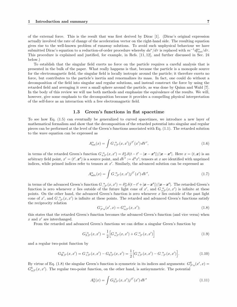
1.3 Green’s functions in flat spacetime
To see how Eq. (1.5) can eventually be generalized to curved spacetimes, we introduce a new layer ofmathematical formalism and show that the decomposition of the retarded potential into singular and regularpieces can be performed at the level of the Green’s functions associated with Eq. (1.1). The retarded solutionto the wave equation can be expressed as
Aαret(x) =
∫G α
+β′(x, x′)jβ
′(x′) dV ′, (1.6)
in terms of the retarded Green’s function G α+β′(x, x
′) = δαβ′δ(t− t′ − |x−x′|)/|x−x′|. Here x = (t,x) is an
arbitrary field point, x′ = (t′,x′) is a source point, and dV ′ := d4x′; tensors at x are identified with unprimedindices, while primed indices refer to tensors at x′. Similarly, the advanced solution can be expressed as
Aαadv(x) =
∫G α−β′(x, x
′)jβ′(x′) dV ′, (1.7)
in terms of the advanced Green’s function G α−β′(x, x
′) = δαβ′δ(t− t′+ |x−x′|)/|x−x′|. The retarded Green’sfunction is zero whenever x lies outside of the future light cone of x′, and G α
+β′(x, x′) is infinite at these
points. On the other hand, the advanced Green’s function is zero whenever x lies outside of the past lightcone of x′, and G α
−β′(x, x′) is infinite at these points. The retarded and advanced Green’s functions satisfy
the reciprocity relationG−β′α(x′, x) = G+
αβ′(x, x′); (1.8)
this states that the retarded Green’s function becomes the advanced Green’s function (and vice versa) whenx and x′ are interchanged.
From the retarded and advanced Green’s functions we can define a singular Green’s function by
G αS β′(x, x
′) =1
2
[G α
+β′(x, x′) +G α
−β′(x, x′)]
(1.9)
and a regular two-point function by
G αR β′(x, x
′) = G α+β′(x, x
′)−G αS β′(x, x
′) =1
2
[G α
+β′(x, x′)−G α
−β′(x, x′)]. (1.10)
By virtue of Eq. (1.8) the singular Green’s function is symmetric in its indices and arguments: GSβ′α(x′, x) =
GSαβ′(x, x
′). The regular two-point function, on the other hand, is antisymmetric. The potential
AαS (x) =
∫G α
S β′(x, x′)jβ
′(x′) dV ′ (1.11)

1 Introduction and summary 8
x
z(u)
retarded
x
z(v)
advanced
Figure 1: In flat spacetime, the retarded potential at x depends on the particle’s state of motion at theretarded point z(u) on the world line; the advanced potential depends on the state of motion at the advancedpoint z(v).
satisfies the wave equation of Eq. (1.1) and is singular on the world line, while
AαR(x) =
∫G α
R β′(x, x′)jβ
′(x′) dV ′ (1.12)
satisfies the homogeneous equation Aα = 0 and is well behaved on the world line.Equation (1.6) implies that the retarded potential at x is generated by a single event in spacetime: the
intersection of the world line and x’s past light cone (see Fig. 1). We shall call this the retarded pointassociated with x and denote it z(u); u is the retarded time, the value of the proper-time parameter at theretarded point. Similarly we find that the advanced potential of Eq. (1.7) is generated by the intersection ofthe world line and the future light cone of the field point x. We shall call this the advanced point associatedwith x and denote it z(v); v is the advanced time, the value of the proper-time parameter at the advancedpoint.
1.4 Green’s functions in curved spacetime
In a curved spacetime with metric gαβ the wave equation for the vector potential becomes
Aα −RαβAβ = −4πjα, (1.13)
where = gαβ∇α∇β is the covariant wave operator and Rαβ is the spacetime’s Ricci tensor; the Lorenzgauge conditions becomes ∇αAα = 0, and ∇α denotes covariant differentiation. Retarded and advancedGreen’s functions can be defined for this equation, and solutions to Eq. (1.13) take the same form as inEqs. (1.6) and (1.7), except that dV ′ now stands for
√−g(x′) d4x′.
The causal structure of the Green’s functions is richer in curved spacetime: While in flat spacetime theretarded Green’s function has support only on the future light cone of x′, in curved spacetime its supportextends inside the light cone as well; G α
+β′(x, x′) is therefore nonzero when x ∈ I+(x′), which denotes the
chronological future of x′. This property reflects the fact that in curved spacetime, electromagnetic wavespropagate not just at the speed of light, but at all speeds smaller than or equal to the speed of light; the delayis caused by an interaction between the radiation and the spacetime curvature. A direct implication of thisproperty is that the retarded potential at x is now generated by the point charge during its entire historyprior to the retarded time u associated with x: the potential depends on the particle’s state of motion forall times τ ≤ u (see Fig. 2).
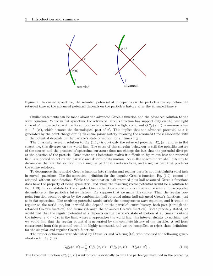
1 Introduction and summary 9
x
z(u)
retarded
z(v)
x
advanced
Figure 2: In curved spacetime, the retarded potential at x depends on the particle’s history before theretarded time u; the advanced potential depends on the particle’s history after the advanced time v.
Similar statements can be made about the advanced Green’s function and the advanced solution to thewave equation. While in flat spacetime the advanced Green’s function has support only on the past lightcone of x′, in curved spacetime its support extends inside the light cone, and G α
−β′(x, x′) is nonzero when
x ∈ I−(x′), which denotes the chronological past of x′. This implies that the advanced potential at x isgenerated by the point charge during its entire future history following the advanced time v associated withx: the potential depends on the particle’s state of motion for all times τ ≥ v.
The physically relevant solution to Eq. (1.13) is obviously the retarded potential Aαret(x), and as in flatspacetime, this diverges on the world line. The cause of this singular behaviour is still the pointlike natureof the source, and the presence of spacetime curvature does not change the fact that the potential divergesat the position of the particle. Once more this behaviour makes it difficult to figure out how the retardedfield is supposed to act on the particle and determine its motion. As in flat spacetime we shall attempt todecompose the retarded solution into a singular part that exerts no force, and a regular part that producesthe entire self-force.
To decompose the retarded Green’s function into singular and regular parts is not a straightforward taskin curved spacetime. The flat-spacetime definition for the singular Green’s function, Eq. (1.9), cannot beadopted without modification: While the combination half-retarded plus half-advanced Green’s functionsdoes have the property of being symmetric, and while the resulting vector potential would be a solution toEq. (1.13), this candidate for the singular Green’s function would produce a self-force with an unacceptabledependence on the particle’s future history. For suppose that we made this choice. Then the regular two-point function would be given by the combination half-retarded minus half-advanced Green’s functions, justas in flat spacetime. The resulting potential would satisfy the homogeneous wave equation, and it would beregular on the world line, but it would also depend on the particle’s entire history, both past (through theretarded Green’s function) and future (through the advanced Green’s function). More precisely stated, wewould find that the regular potential at x depends on the particle’s state of motion at all times τ outsidethe interval u < τ < v; in the limit where x approaches the world line, this interval shrinks to nothing, andwe would find that the regular potential is generated by the complete history of the particle. A self-forceconstructed from this potential would be highly noncausal, and we are compelled to reject these definitionsfor the singular and regular Green’s functions.
The proper definitions were identified by Detweiler and Whiting [13], who proposed the following gener-alization to Eq. (1.9):
G αS β′(x, x
′) =1
2
[G α
+β′(x, x′) +G α
−β′(x, x′)−Hα
β′(x, x′)]. (1.14)
The two-point function Hαβ′(x, x
′) is introduced specifically to cure the pathology described in the preceding

1 Introduction and summary 10
x
z(u)
singular
x
z(v)
regular
Figure 3: In curved spacetime, the singular potential at x depends on the particle’s history during theinterval u ≤ τ ≤ v; for the regular potential the relevant interval is −∞ < τ ≤ v.
paragraph. It is symmetric in its indices and arguments, so that GSαβ′(x, x
′) will be also (since the retardedand advanced Green’s functions are still linked by a reciprocity relation); and it is a solution to the homo-geneous wave equation, Hα
β′(x, x′) − Rαγ(x)Hγ
β′(x, x′) = 0, so that the singular, retarded, and advanced
Green’s functions will all satisfy the same wave equation. Furthermore, and this is its key property, thetwo-point function is defined to agree with the advanced Green’s function when x is in the chronological pastof x′: Hα
β′(x, x′) = G α
−β′(x, x′) when x ∈ I−(x′). This ensures that G α
S β′(x, x′) vanishes when x is in the
chronological past of x′. In fact, reciprocity implies that Hαβ′(x, x
′) will also agree with the retarded Green’sfunction when x is in the chronological future of x′, and it follows that the symmetric Green’s functionvanishes also when x is in the chronological future of x′.
The potential AαS (x) constructed from the singular Green’s function can now be seen to depend on theparticle’s state of motion at times τ restricted to the interval u ≤ τ ≤ v (see Fig. 3). Because this potentialsatisfies Eq. (1.13), it is just as singular as the retarded potential in the vicinity of the world line. Andbecause the singular Green’s function is symmetric in its arguments, the singular potential can be shown toexert no force on the charged particle. (This requires a lengthy analysis that will be presented in the bulkof the paper.)
The Detweiler-Whiting [13] definition for the regular two-point function is then
G αR β′(x, x
′) = G α+β′(x, x
′)−G αS β′(x, x
′) =1
2
[G α
+β′(x, x′)−G α
−β′(x, x′) +Hα
β′(x, x′)]. (1.15)
The potential AαR(x) constructed from this depends on the particle’s state of motion at all times τ priorto the advanced time v: τ ≤ v. Because this potential satisfies the homogeneous wave equation, it is wellbehaved on the world line and its action on the point charge is well defined. And because the singularpotential AαS (x) can be shown to exert no force on the particle, we conclude that AαR(x) alone is responsiblefor the self-force.
From the regular potential we form an electromagnetic field tensor FRαβ = ∇αAR
β − ∇βARα and the
curved-spacetime generalization to Eq. (1.4) is
maµ = f extµ + eFR
µνuν , (1.16)
where uµ = dzµ/dτ is again the charge’s four-velocity, but aµ = Duµ/dτ is now its covariant acceleration.
1.5 World line and retarded coordinates
To flesh out the ideas contained in the preceding subsection we add yet another layer of mathematicalformalism and construct a convenient coordinate system to chart a neighbourhood of the particle’s world

1 Introduction and summary 11
line. In the next subsection we will display explicit expressions for the retarded, singular, and regular fieldsof a point electric charge.
Let γ be the world line of a point particle in a curved spacetime. It is described by parametric relationszµ(τ) in which τ is proper time. Its tangent vector is uµ = dzµ/dτ and its acceleration is aµ = Duµ/dτ ; weshall also encounter aµ := Daµ/dτ .
On γ we erect an orthonormal basis that consists of the four-velocity uµ and three spatial vectors eµalabelled by a frame index a = (1, 2, 3). These vectors satisfy the relations gµνu
µuν = −1, gµνuµeνa = 0, and
gµνeµaeνb = δab. We take the spatial vectors to be Fermi-Walker transported on the world line: Deµa/dτ =
aauµ, where
aa(τ) = aµeµa (1.17)
are frame components of the acceleration vector; it is easy to show that Fermi-Walker transport preservesthe orthonormality of the basis vectors. We shall use the tetrad to decompose various tensors evaluated onthe world line. An example was already given in Eq. (1.17) but we shall also encounter frame componentsof the Riemann tensor,
Ra0b0(τ) = Rµλνρeµau
λeνbuρ, Ra0bc(τ) = Rµλνρe
µau
λeνb eρc , Rabcd(τ) = Rµλνρe
µaeλb eνc eρd, (1.18)
as well as frame components of the Ricci tensor,
R00(τ) = Rµνuµuν , Ra0(τ) = Rµνe
µau
ν , Rab(τ) = Rµνeµaeνb . (1.19)
We shall use δab = diag(1, 1, 1) and its inverse δab = diag(1, 1, 1) to lower and raise frame indices, respectively.Consider a point x in a neighbourhood of the world line γ. We assume that x is sufficiently close to the
world line that a unique geodesic links x to any neighbouring point z on γ. The two-point function σ(x, z),known as Synge’s world function [14], is numerically equal to half the squared geodesic distance betweenz and x; it is positive if x and z are spacelike related, negative if they are timelike related, and σ(x, z) iszero if x and z are linked by a null geodesic. We denote its gradient ∂σ/∂zµ by σµ(x, z), and −σµ gives ameaningful notion of a separation vector (pointing from z to x).
To construct a coordinate system in this neighbourhood we locate the unique point x′ := z(u) on γ whichis linked to x by a future-directed null geodesic (this geodesic is directed from x′ to x); we shall refer to x′ asthe retarded point associated with x, and u will be called the retarded time. To tensors at x′ we assign indicesα′, β′, . . . ; this will distinguish them from tensors at a generic point z(τ) on the world line, to which wehave assigned indices µ, ν, . . . . We have σ(x, x′) = 0 and −σα′(x, x′) is a null vector that can be interpretedas the separation between x′ and x.
The retarded coordinates of the point x are (u, xa), where xa = −eaα′σα′
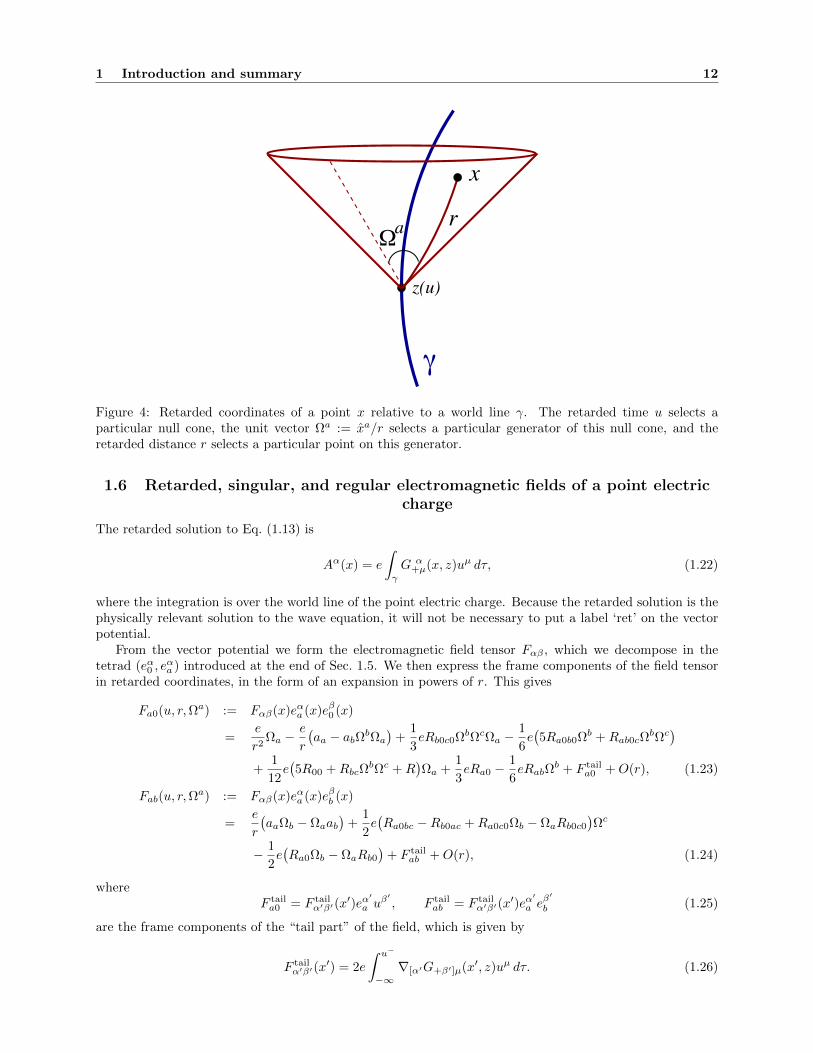
are the frame components of theseparation vector. They come with a straightforward interpretation (see Fig. 4). The invariant quantity
r :=√δabxaxb = uα′σ
α′ (1.20)
is an affine parameter on the null geodesic that links x to x′; it can be loosely interpreted as the time delaybetween x and x′ as measured by an observer moving with the particle. This therefore gives a meaningfulnotion of distance between x and the retarded point, and we shall call r the retarded distance between x andthe world line. The unit vector
Ωa = xa/r (1.21)
is constant on the null geodesic that links x to x′. Because Ωa is a different constant on each null geodesicthat emanates from x′, keeping u fixed and varying Ωa produces a congruence of null geodesics that generatethe future light cone of the point x′ (the congruence is hypersurface orthogonal). Each light cone can thusbe labelled by its retarded time u, each generator on a given light cone can be labelled by its direction vectorΩa, and each point on a given generator can be labelled by its retarded distance r. We therefore have a goodcoordinate system in a neighbourhood of γ.
To tensors at x we assign indices α, β, . . . . These tensors will be decomposed in a tetrad (eα0 , eαa ) that is
constructed as follows: Given x we locate its associated retarded point x′ on the world line, as well as thenull geodesic that links these two points; we then take the tetrad (uα
′, eα
′
a ) at x′ and parallel transport it tox along the null geodesic to obtain (eα0 , e
αa ).
1 Introduction and summary 12
a r
x
z(u)
Figure 4: Retarded coordinates of a point x relative to a world line γ. The retarded time u selects aparticular null cone, the unit vector Ωa := xa/r selects a particular generator of this null cone, and theretarded distance r selects a particular point on this generator.
1.6 Retarded, singular, and regular electromagnetic fields of a point electriccharge
The retarded solution to Eq. (1.13) is
Aα(x) = e
∫γ
G α+µ(x, z)uµ dτ, (1.22)
where the integration is over the world line of the point electric charge. Because the retarded solution is thephysically relevant solution to the wave equation, it will not be necessary to put a label ‘ret’ on the vectorpotential.
From the vector potential we form the electromagnetic field tensor Fαβ , which we decompose in thetetrad (eα0 , e
αa ) introduced at the end of Sec. 1.5. We then express the frame components of the field tensor
in retarded coordinates, in the form of an expansion in powers of r. This gives
Fa0(u, r,Ωa) := Fαβ(x)eαa (x)eβ0 (x)
=e
r2Ωa −
e
r
(aa − abΩbΩa
)+
1
3eRb0c0ΩbΩcΩa −
1
6e(5Ra0b0Ωb +Rab0cΩ
bΩc)
+1
12e(5R00 +RbcΩ
bΩc +R)Ωa +
1
3eRa0 −
1
6eRabΩ
b + F taila0 +O(r), (1.23)
Fab(u, r,Ωa) := Fαβ(x)eαa (x)eβb (x)
=e
r
(aaΩb − Ωaab
)+
1
2e(Ra0bc −Rb0ac +Ra0c0Ωb − ΩaRb0c0
)Ωc
− 1
2e(Ra0Ωb − ΩaRb0
)+ F tail
ab +O(r), (1.24)
whereF taila0 = F tail
α′β′(x′)eα
′
a uβ′ , F tail
ab = F tailα′β′(x
′)eα′
a eβ′
b (1.25)
are the frame components of the “tail part” of the field, which is given by
F tailα′β′(x
′) = 2e
∫ u−
−∞∇[α′G+β′]µ(x′, z)uµ dτ. (1.26)
1 Introduction and summary 13
In these expressions, all tensors (or their frame components) are evaluated at the retarded point x′ := z(u)associated with x; for example, aa := aa(u) := aα′e
α′
a . The tail part of the electromagnetic field tensor iswritten as an integral over the portion of the world line that corresponds to the interval −∞ < τ ≤ u− :=u− 0+; this represents the past history of the particle. The integral is cut short at u− to avoid the singularbehaviour of the retarded Green’s function when z(τ) coincides with x′; the portion of the Green’s functioninvolved in the tail integral is smooth, and the singularity at coincidence is completely accounted for by theother terms in Eqs. (1.23) and (1.24).
The expansion of Fαβ(x) near the world line does indeed reveal many singular terms. We first recognizeterms that diverge when r → 0; for example the Coulomb field Fa0 diverges as r−2 when we approach theworld line. But there are also terms that, though they stay bounded in the limit, possess a directionalambiguity at r = 0; for example Fab contains a term proportional to Ra0bcΩ
c whose limit depends on thedirection of approach.
This singularity structure is perfectly reproduced by the singular field F Sαβ obtained from the potential
AαS (x) = e
∫γ
G αSµ(x, z)uµ dτ, (1.27)
where G αSµ(x, z) is the singular Green’s function of Eq. (1.14). Near the world line the singular field is given
by
F Sa0(u, r,Ωa) := F S
αβ(x)eαa (x)eβ0 (x)
=e
r2Ωa −
e
r
(aa − abΩbΩa
)− 2
3eaa +
1
3eRb0c0ΩbΩcΩa −
1
6e(5Ra0b0Ωb +Rab0cΩ
bΩc)
+1
12e(5R00 +RbcΩ
bΩc +R)Ωa −
1
6eRabΩ
b +O(r), (1.28)
F Sab(u, r,Ω
a) := F Sαβ(x)eαa (x)eβb (x)
=e
r
(aaΩb − Ωaab
)+
1
2e(Ra0bc −Rb0ac +Ra0c0Ωb − ΩaRb0c0
)Ωc
− 1
2e(Ra0Ωb − ΩaRb0
)+O(r). (1.29)
Comparison of these expressions with Eqs. (1.23) and (1.24) does indeed reveal that all singular terms areshared by both fields.
The difference between the retarded and singular fields defines the regular field FRαβ(x). Its frame com-
ponents are
FRa0 =
2
3eaa +
1
3eRa0 + F tail
a0 +O(r), (1.30)
FRab = F tail
ab +O(r), (1.31)
and at x′ the regular field becomes
FRα′β′ = 2eu[α′
(gβ′]γ′ + uβ′]uγ′
)(2
3aγ′+
1
3Rγ′
δ′uδ′)
+ F tailα′β′ , (1.32)
where aγ′
= Daγ′/dτ is the rate of change of the acceleration vector, and where the tail term was given by
Eq. (1.26). We see that FRαβ(x) is a regular tensor field, even on the world line.
1.7 Motion of an electric charge in curved spacetime
We have argued in Sec. 1.4 that the self-force acting on a point electric charge is produced by the regularfield, and that the charge’s equations of motion should take the form of maµ = f ext
µ + eFRµνu
ν , where f extµ is
an external force also acting on the particle. Substituting Eq. (1.32) gives
maµ = fµext + e2(δµν + uµuν
)( 2
3m
Dfνext
dτ+
1
3Rνλu
λ
)+ 2e2uν
∫ τ−
−∞∇[µG
ν]+λ′
(z(τ), z(τ ′)
)uλ′dτ ′, (1.33)

1 Introduction and summary 14
in which all tensors are evaluated at z(τ), the current position of the particle on the world line. The primedindices in the tail integral refer to a point z(τ ′) which represents a prior position; the integration is cut shortat τ ′ = τ− := τ − 0+ to avoid the singular behaviour of the retarded Green’s function at coincidence. Toget Eq. (1.33) we have reduced the order of the differential equation by replacing aν with m−1fνext on theright-hand side; this procedure was explained at the end of Sec. 1.2.
Equation (1.33) is the result that was first derived by DeWitt and Brehme [4] and later corrected byHobbs [5]. (The original version of the equation did not include the Ricci-tensor term.) In flat spacetime theRicci tensor is zero, the tail integral disappears (because the Green’s function vanishes everywhere withinthe domain of integration), and Eq. (1.33) reduces to Dirac’s result of Eq. (1.5). In curved spacetime theself-force does not vanish even when the electric charge is moving freely, in the absence of an external force:it is then given by the tail integral, which represents radiation emitted earlier and coming back to the particleafter interacting with the spacetime curvature. This delayed action implies that in general, the self-force isnonlocal in time: it depends not only on the current state of motion of the particle, but also on its pasthistory. Lest this behaviour should seem mysterious, it may help to keep in mind that the physical processthat leads to Eq. (1.33) is simply an interaction between the charge and a free electromagnetic field FR
αβ ; itis this field that carries the information about the charge’s past.
1.8 Motion of a scalar charge in curved spacetime
The dynamics of a point scalar charge can be formulated in a way that stays fairly close to the electromagnetictheory. The particle’s charge q produces a scalar field Φ(x) which satisfies a wave equation(
− ξR)Φ = −4πµ (1.34)
that is very similar to Eq. (1.13). Here, R is the spacetime’s Ricci scalar, and ξ is an arbitrary couplingconstant; the scalar charge density µ(x) is given by a four-dimensional Dirac functional supported on theparticle’s world line γ. The retarded solution to the wave equation is
Φ(x) = q
∫γ
G+(x, z) dτ, (1.35)
where G+(x, z) is the retarded Green’s function associated with Eq. (1.34). The field exerts a force on theparticle, whose equations of motion are
maµ = q(gµν + uµuν
)∇νΦ, (1.36)
where m is the particle’s mass; this equation is very similar to the Lorentz-force law. But the dynamicsof a scalar charge comes with a twist: If Eqs. (1.34) and (1.36) are to follow from a variational principle,the particle’s mass should not be expected to be a constant of the motion. It is found instead to satisfy thedifferential equation
dm
dτ= −quµ∇µΦ, (1.37)
and in general m will vary with proper time. This phenomenon is linked to the fact that a scalar field haszero spin: the particle can radiate monopole waves and the radiated energy can come at the expense of therest mass.
The scalar field of Eq. (1.35) diverges on the world line and its singular part ΦS(x) must be removedbefore Eqs. (1.36) and (1.37) can be evaluated. This procedure produces the regular field ΦR(x), and it isthis field (which satisfies the homogeneous wave equation) that gives rise to a self-force. The gradient of theregular field takes the form of
∇µΦR = − 1
12(1− 6ξ)qRuµ + q
(gµν + uµuν
)(1
3aν +
1
6Rνλu
λ
)+ Φtail
µ (1.38)
when it is evaluated on the world line. The last term is the tail integral
Φtailµ = q
∫ τ−
−∞∇µG+
(z(τ), z(τ ′)
)dτ ′, (1.39)

1 Introduction and summary 15
and this brings the dependence on the particle’s past.Substitution of Eq. (1.38) into Eqs. (1.36) and (1.37) gives the equations of motion of a point scalar
charge. (At this stage we introduce an external force fµext and reduce the order of the differential equation.)The acceleration is given by
maµ = fµext + q2(δµν + uµuν
)[ 1
3m
Dfνext
dτ+
1
6Rνλu
λ +
∫ τ−
−∞∇νG+
(z(τ), z(τ ′)
)dτ ′
](1.40)
and the mass changes according to
dm
dτ= − 1
12(1− 6ξ)q2R− q2uµ
∫ τ−
−∞∇µG+
(z(τ), z(τ ′)
)dτ ′. (1.41)
These equations were first derived by Quinn [8]. (His analysis was restricted to a minimally coupled scalarfield, so that ξ = 0 in his expressions. We extended Quinn’s results to an arbitrary coupling counstant forthis review.)
In flat spacetime the Ricci-tensor term and the tail integral disappear and Eq. (1.40) takes the form ofEq. (1.5) with q2/(3m) replacing the factor of 2e2/(3m). In this simple case Eq. (1.41) reduces to dm/dτ = 0and the mass is in fact a constant. This property remains true in a conformally flat spacetime when the waveequation is conformally invariant (ξ = 1/6): in this case the Green’s function possesses only a light-conepart and the right-hand side of Eq. (1.41) vanishes. In generic situations the mass of a point scalar chargewill vary with proper time.
1.9 Motion of a point mass, or a small body, in a background spacetime
The case of a point mass moving in a specified background spacetime presents itself with a serious conceptualchallenge, as the fundamental equations of the theory are nonlinear and the very notion of a “point mass”is somewhat misguided. Nevertheless, to the extent that the perturbation hαβ(x) created by the point masscan be considered to be “small”, the problem can be formulated in close analogy with what was presentedbefore.
We take the metric gαβ of the background spacetime to be a solution of the Einstein field equations invacuum. (We impose this condition globally.) We describe the gravitational perturbation produced by apoint particle of mass m in terms of trace-reversed potentials γαβ defined by
γαβ = hαβ −1
2
(gγδhγδ
)gαβ , (1.42)
where hαβ is the difference between gαβ , the actual metric of the perturbed spacetime, and gαβ . Thepotentials satisfy the wave equation
γαβ + 2R α βγ δ γ
γδ = −16πTαβ +O(m2) (1.43)
together with the Lorenz gauge condition γαβ;β = 0. Here and below, covariant differentiation refers to
a connection that is compatible with the background metric, = gαβ∇α∇β is the wave operator for thebackground spacetime, and Tαβ is the energy-momentum tensor of the point mass; this is given by a Diracdistribution supported on the particle’s world line γ. The retarded solution is
γαβ(x) = 4m
∫γ
G αβ+ µν(x, z)uµuν dτ +O(m2), (1.44)
where G αβ+ µν(x, z) is the retarded Green’s function associated with Eq. (1.43). The perturbation hαβ(x) can
be recovered by inverting Eq. (1.42).Equations of motion for the point mass can be obtained by formally demanding that the motion be
geodesic in the perturbed spacetime with metric gαβ = gαβ + hαβ . After a mapping to the backgroundspacetime, the equations of motion take the form of
aµ = −1
2
(gµν + uµuν
)(2hνλ;ρ − hλρ;ν
)uλuρ +O(m2). (1.45)

1 Introduction and summary 16
The acceleration is thus proportional to m; in the test-mass limit the world line of the particle is a geodesicof the background spacetime.
We now remove hSαβ(x) from the retarded perturbation and postulate that it is the regular field hR
αβ(x)
that should act on the particle. (Note that γSαβ satisfies the same wave equation as the retarded potentials,
but that γRαβ is a free gravitational field that satisfies the homogeneous wave equation.) On the world line
we havehRµν;λ = −4m
(u(µRν)ρλξ +Rµρνξuλ
)uρuξ + htail
µνλ, (1.46)
where the tail term is given by
htailµνλ = 4m
∫ τ−
−∞∇λ(G+µνµ′ν′ −
1
2gµνG
ρ+ ρµ′ν′
)(z(τ), z(τ ′)
)uµ′uν′dτ ′. (1.47)
When Eq. (1.46) is substituted into Eq. (1.45) we find that the terms that involve the Riemann tensor cancelout, and we are left with
aµ = −1
2
(gµν + uµuν
)(2htail
νλρ − htailλρν
)uλuρ +O(m2). (1.48)
Only the tail integral appears in the final form of the equations of motion. It involves the current position z(τ)of the particle, at which all tensors with unprimed indices are evaluated, as well as all prior positions z(τ ′),at which tensors with primed indices are evaluated. As before the integral is cut short at τ ′ = τ− := τ − 0+
to avoid the singular behaviour of the retarded Green’s function at coincidence.The equations of motion of Eq. (1.48) were first derived by Mino, Sasaki, and Tanaka [6], and then
reproduced with a different analysis by Quinn and Wald [7]. They are now known as the MiSaTaQuWaequations of motion. As noted by these authors, the MiSaTaQuWa equation has the appearance of thegeodesic equation in a metric gαβ + htail
αβ . Detweiler and Whiting [13] have contributed the more compelling
interpretation that the motion is actually geodesic in a spacetime with metric gαβ + hRαβ . The distinction is
important: Unlike the first version of the metric, the Detweiler-Whiting metric is regular on the world lineand satisfies the Einstein field equations in vacuum; and because it is a solution to the field equations, it canbe viewed as a physical metric — specifically, the metric of the background spacetime perturbed by a freefield produced by the particle at an earlier stage of its history.
While Eq. (1.48) does indeed give the correct equations of motion for a small mass m moving in abackground spacetime with metric gαβ , the derivation outlined here leaves much to be desired — to whatextent should we trust an analysis based on the existence of a point mass? As a partial answer to this question,Mino, Sasaki, and Tanaka [6] produced an alternative derivation of their result, which involved a smallnonrotating black hole instead of a point mass. In this alternative derivation, the metric of the black holeperturbed by the tidal gravitational field of the external universe is matched to the metric of the backgroundspacetime perturbed by the moving black hole. Demanding that this metric be a solution to the vacuum fieldequations determines the motion of the black hole: it must move according to Eq. (1.48). This alternativederivation (which was given a different implementation in Ref. [15]) is entirely free of singularities (exceptdeep within the black hole), and it suggests that the MiSaTaQuWa equations can be trusted to describe themotion of any gravitating body in a curved background spacetime (so long as the body’s internal structurecan be ignored). This derivation, however, was limited to the case of a non-rotating black hole, and it reliedon a number of unjustified and sometimes unstated assumptions [16–18]. The conclusion was made firmby the more rigorous analysis of Gralla and Wald [16] (as extended by Pound [17]), who showed that theMiSaTaQuWa equations apply to any sufficiently compact body of arbitrary internal structure.
It is important to understand that unlike Eqs. (1.33) and (1.40), which are true tensorial equations,Eq. (1.48) reflects a specific choice of coordinate system and its form would not be preserved under acoordinate transformation. In other words, the MiSaTaQuWa equations are not gauge invariant, and theydepend upon the Lorenz gauge condition γαβ;β = O(m2). Barack and Ori [19] have shown that under acoordinate transformation of the form xα → xα + ξα, where xα are the coordinates of the backgroundspacetime and ξα is a smooth vector field of order m, the particle’s acceleration changes according toaµ → aµ + a[ξ]µ, where
a[ξ]µ =(δµν + uµuν
)(D2ξν
dτ2+Rνρωλu
ρξωuλ)
(1.49)
1 Introduction and summary 17
is the “gauge acceleration”; D2ξν/dτ2 = (ξν;µuµ);ρu
ρ is the second covariant derivative of ξν in the directionof the world line. This implies that the particle’s acceleration can be altered at will by a gauge transformation;ξα could even be chosen so as to produce aµ = 0, making the motion geodesic after all. This observationprovides a dramatic illustration of the following point: The MiSaTaQuWa equations of motion are not gaugeinvariant and they cannot by themselves produce a meaningful answer to a well-posed physical question; toobtain such answers it is necessary to combine the equations of motion with the metric perturbation hαβ soas to form gauge-invariant quantities that will correspond to direct observables. This point is very importantand cannot be over-emphasized.
The gravitational self-force possesses a physical significance that is not shared by its scalar and electro-magnetic analogues, because the motion of a small body in the strong gravitational field of a much largerbody is a problem of direct relevance to gravitational-wave astronomy. Indeed, extreme-mass-ratio inspirals,involving solar-mass compact objects moving around massive black holes of the sort found in galactic cores,have been identified as promising sources of low-frequency gravitational waves for space-based interferomet-ric detectors such as the proposed Laser Interferometer Space Antenna (LISA [20]). These systems involvehighly eccentric, nonequatorial, and relativistic orbits around rapidly rotating black holes, and the wavesproduced by such orbital motions are rich in information concerning the strongest gravitational fields inthe Universe. This information will be extractable from the LISA data stream, but the extraction dependson sophisticated data-analysis strategies that require a detailed and accurate modeling of the source. Thismodeling involves formulating the equations of motion for the small body in the field of the rotating blackhole, as well as a consistent incorporation of the motion into a wave-generation formalism. In short, theextraction of this wealth of information relies on a successful evaluation of the gravitational self-force.
The finite-mass corrections to the orbital motion are important. For concreteness, let us assume that theorbiting body is a black hole of mass m = 10 M and that the central black hole has a mass M = 106 M.Let us also assume that the small black hole is in the deep field of the large hole, near the innermost stablecircular orbit, so that its orbital period P is of the order of minutes. The gravitational waves produced bythe orbital motion have frequencies f of the order of the mHz, which is well within LISA’s frequency band.The radiative losses drive the orbital motion toward a final plunge into the large black hole; this occursover a radiation-reaction timescale (M/m)P of the order of a year, during which the system will go througha number of wave cycles of the order of M/m = 105. The role of the gravitational self-force is preciselyto describe this orbital evolution toward the final plunge. While at any given time the self-force providesfractional corrections of order m/M = 10−5 to the motion of the small black hole, these build up over anumber of orbital cycles of order M/m = 105 to produce a large cumulative effect. As will be discussed insome detail in Sec. 2.6, the gravitational self-force is important, because it drives large secular changes inthe orbital motion of an extreme-mass-ratio binary.
1.10 Case study: static electric charge in Schwarzschild spacetime
One of the first self-force calculations ever performed for a curved spacetime was presented by Smith andWill [21]. They considered an electric charge e held in place at position r = r0 outside a Schwarzschildblack hole of mass M . Such a static particle must be maintained in position with an external force thatcompensates for the black hole’s attraction. For a particle without electric charge this force is directedoutward, and its radial component in Schwarzschild coordinates is given by frext = 1
2mf′, where m is the
particle’s mass, f := 1− 2M/r0 is the usual metric factor, and a prime indicates differentiation with respectto r0, so that f ′ = 2M/r2
0. Smith and Will found that for a particle of charge e, the external force is giveninstead by frext = 1
2mf′ − e2Mf1/2/r3
0. The second term is contributed by the electromagnetic self-force,and implies that the external force is smaller for a charged particle. This means that the electromagneticself-force acting on the particle is directed outward and given by
frself =e2M
r30
f1/2. (1.50)
This is a repulsive force. It was shown by Zel’nikov and Frolov [22] that the same expression applies to astatic charge outside a Reissner-Nordstrom black hole of mass M and charge Q, provided that f is replacedby the more general expression f = 1− 2M/r0 +Q2/r2
0.
1 Introduction and summary 18
The repulsive nature of the electromagnetic self-force acting on a static charge outside a black hole isunexpected. In an attempt to gain some intuition about this result, it is useful to recall that a black-holehorizon always acts as perfect conductor, because the electrostatic potential ϕ := −At is necessarily uniformacross its surface. It is then tempting to imagine that the self-force should result from a fictitious distributionof induced charge on the horizon, and that it could be estimated on the basis of an elementary model involvinga spherical conductor. Let us, therefore, calculate the electric field produced by a point charge e situatedoutside a spherical conductor of radius R. The charge is placed at a distance r0 from the centre of theconductor, which is taken at first to be grounded. The electrostatic potential produced by the charge caneasily be obtained with the method of images. It is found that an image charge e′ = −eR/r0 is situated ata distance r′0 = R2/r0 from the centre of the conductor, and the potential is given by ϕ = e/s+ e′/s′, wheres is the distance to the charge, while s′ is the distance to the image charge. The first term can be identifiedwith the singular potential ϕS, and the associated electric field exerts no force on the point charge. Thesecond term is the regular potential ϕR, and the associated field is entirely responsible for the self-force. Theregular electric field is ErR = −∂rϕR, and the self-force is frself = eErR. A simple computation returns
frself = − e2R
r30(1−R2/r2
0). (1.51)
This is an attractive self-force, because the total induced charge on the conducting surface is equal to e′,which is opposite in sign to e. With R identified with M up to a numerical factor, we find that our intuitionhas produced the expected factor of e2M/r3
0, but that it gives rise to the wrong sign for the self-force. Anattempt to refine this computation by removing the net charge e′ on the conductor (to mimic more closelythe black-hole horizon, which cannot support a net charge) produces a wrong dependence on r0 in additionto the same wrong sign. In this case the conductor is maintained at a constant potential φ0 = −e′/R, andthe situation involves a second image charge −e′ situated at r = 0. It is easy to see that in this case,
frself = − e2R3
r50(1−R2/r2
0). (1.52)
This is still an attractive force, which is weaker than the force of Eq. (1.51) by a factor of (R/r0)2; the forceis now exerted by an image dipole instead of a single image charge.
The computation of the self-force in the black-hole case is almost as straightforward. The exact solutionto Maxwell’s equations that describes a point charge e situated r = r0 and θ = 0 in the Schwarzschildspacetime is given by
ϕ = ϕS + ϕR, (1.53)
where
ϕS =e
r0r
(r −M)(r0 −M)−M2 cos θ[(r −M)2 − 2(r −M)(r0 −M) cos θ + (r0 −M)2 −M2 sin2 θ
]1/2 , (1.54)
is the solution first discovered by Copson in 1928 [23], while
ϕR =eM/r0
r(1.55)
is the monopole field that was added by Linet [24] to obtain the correct asymptotic behaviour ϕ ∼ e/rwhen r is much larger than r0. It is easy to see that Copson’s potential behaves as e(1−M/r0)/r at largedistances, which reveals that in addition to e, ϕS comes with an additional (and unphysical) charge −eM/r0
situated at r = 0. This charge must be removed by adding to ϕS a potential that (i) is a solution to thevacuum Maxwell equations, (ii) is regular everywhere except at r = 0, and (iii) carries the opposite charge+eM/r0; this potential must be a pure monopole, because higher multipoles would produce a singularity onthe horizon, and it is given uniquely by ϕR. The Copson solution was generalized to Reissner-Nordstromspacetime by Leaute and Linet [25], who also showed that the regular potential of Eq. (1.55) requires nomodification.
The identification of Copson’s potential with the singular potential ϕS is motivated by the fact that itsassociated electric field F S
tr = ∂rϕS is isotropic around the charge e and therefore exerts no force. The

1 Introduction and summary 19
self-force comes entirely from the monopole potential, which describes a (fictitious) charge +eM/r0 situatedat r = 0. Because this charge is of the same sign as the original charge e, the self-force is repulsive. Moreprecisely stated, we find that the regular piece of the electric field is given by
FRtr = −eM/r0
r2, (1.56)
and that it produces the self-force of Eq. (1.50). The simple picture described here, in which the electromag-netic self-force is produced by a fictitious charge eM/r0 situated at the centre of the black hole, is not easilyextracted from the derivation presented originally by Smith and Will [21]. To the best of our knowledge, themonopolar origin of the self-force was first noticed by Alan Wiseman [26]. (In his paper, Wiseman computedthe scalar self-force acting on a static particle in Schwarzschild spacetime, and found a zero answer. In thiscase, the analogue of the Copson solution for the scalar potential happens to satisfy the correct asymptoticconditions, and there is no need to add another solution to it. Because the scalar potential is precisely equalto the singular potential, the self-force vanishes.)
We should remark that the identification of ϕS and ϕR with the Detweiler-Whiting singular and reg-ular fields, respectively, is a matter of conjecture. Although ϕS and ϕR satisfy the essential properties ofthe Detweiler-Whiting decomposition — being, respectively, a regular homogenous solution and a singu-lar solution sourced by the particle — one should accept the possibility that they may not be the actualDetweiler-Whiting fields. It is a topic for future research to investigate the precise relation between theCopson field and the Detweiler-Whiting singular field.
It is instructive to compare the electromagnetic self-force produced by the presence of a grounded con-ductor to the self-force produced by the presence of a black hole. In the case of a conductor, the total inducedcharge on the conducting surface is e′ = −eR/r0, and it is this charge that is responsible for the attractiveself-force; the induced charge is supplied by the electrodes that keep the conductor grounded. In the case ofa black hole, there is no external apparatus that can supply such a charge, and the total induced charge onthe horizon necessarily vanishes. The origin of the self-force is therefore very different in this case. As wehave seen, the self-force is produced by a fictitious charge eM/r0 situated at the centre of black hole; andbecause this charge is positive, the self-force is repulsive.
1.11 Organization of this review
After a detailed review of the literature in Sec. 2, the main body of the review begins in Part I (Secs. 3to 7) with a description of the general theory of bitensors, the name designating tensorial functions of twopoints in spacetime. We introduce Synge’s world function σ(x, x′) and its derivatives in Sec. 3, the parallelpropagator gαα′(x, x
′) in Sec. 5, and the van Vleck determinant ∆(x, x′) in Sec. 7. An important portion ofthe theory (covered in Secs. 4 and 6) is concerned with the expansion of bitensors when x is very close to x′;expansions such as those displayed in Eqs. (1.23) and (1.24) are based on these techniques. The presentationin Part I borrows heavily from Synge’s book [14] and the article by DeWitt and Brehme [4]. These twosources use different conventions for the Riemann tensor, and we have adopted Synge’s conventions (whichagree with those of Misner, Thorne, and Wheeler [27]). The reader is therefore warned that formulae derivedin Part I may look superficially different from those found in DeWitt and Brehme.
In Part II (Secs. 8 to 11) we introduce a number of coordinate systems that play an important role inlater parts of the review. As a warmup exercise we first construct (in Sec. 8) Riemann normal coordinatesin a neighbourhood of a reference point x′. We then move on (in Sec. 9) to Fermi normal coordinates [28],which are defined in a neighbourhood of a world line γ. The retarded coordinates, which are also basedat a world line and which were briefly introduced in Sec. 1.5, are covered systematically in Sec. 10. Therelationship between Fermi and retarded coordinates is worked out in Sec. 11, which also locates the advancedpoint z(v) associated with a field point x. The presentation in Part II borrows heavily from Synge’s book[14]. In fact, we are much indebted to Synge for initiating the construction of retarded coordinates in aneighbourhood of a world line. We have implemented his program quite differently (Synge was interestedin a large neighbourhood of the world line in a weakly curved spacetime, while we are interested in a smallneighbourhood in a strongly curved spacetime), but the idea is originally his.
In Part III (Secs. 12 to 16) we review the theory of Green’s functions for (scalar, vectorial, and tensorial)wave equations in curved spacetime. We begin in Sec. 12 with a pedagogical introduction to the retarded

1 Introduction and summary 20
and advanced Green’s functions for a massive scalar field in flat spacetime; in this simple context the all-important Hadamard decomposition [29] of the Green’s function into “light-cone” and “tail” parts can bedisplayed explicitly. The invariant Dirac functional is defined in Sec. 13 along with its restrictions on thepast and future null cones of a reference point x′. The retarded, advanced, singular, and regular Green’sfunctions for the scalar wave equation are introduced in Sec. 14. In Secs. 15 and 16 we cover the vectorialand tensorial wave equations, respectively. The presentation in Part III is based partly on the paper byDeWitt and Brehme [4], but it is inspired mostly by Friedlander’s book [30]. The reader should be warnedthat in one important aspect, our notation differs from the notation of DeWitt and Brehme: While theydenote the tail part of the Green’s function by −v(x, x′), we have taken the liberty of eliminating the sillyminus sign and call it instead +V (x, x′). The reader should also note that all our Green’s functions arenormalized in the same way, with a factor of −4π multiplying a four-dimensional Dirac functional of theright-hand side of the wave equation. (The gravitational Green’s function is sometimes normalized with a−16π on the right-hand side.)
In Part IV (Secs. 17 to 19) we compute the retarded, singular, and regular fields associated with a pointscalar charge (Sec. 17), a point electric charge (Sec. 18), and a point mass (Sec. 19). We provide two differentderivations for each of the equations of motion. The first type of derivation was outlined previously: Wefollow Detweiler and Whiting [13] and postulate that only the regular field exerts a force on the particle.In the second type of derivation we take guidance from Quinn and Wald [7] and postulate that the netforce exerted on a point particle is given by an average of the retarded field over a surface of constantproper distance orthogonal to the world line — this rest-frame average is easily carried out in Fermi normalcoordinates. The averaged field is still infinite on the world line, but the divergence points in the directionof the acceleration vector and it can thus be removed by mass renormalization. Such calculations show thatwhile the singular field does not affect the motion of the particle, it nonetheless contributes to its inertia.
In Part V (Secs. 20 to 23), we show that at linear order in the body’s mass m, an extended body behavesjust as a point mass, and except for the effects of the body’s spin, the world line representing its meanmotion is governed by the MiSaTaQuWa equation. At this order, therefore, the picture of a point particleinteracting with its own field, and the results obtained from this picture, is justified. Our derivation utilizesthe method of matched asymptotic expansions, with an inner expansion accurate near the body and an outerexpansion accurate everywhere else. The equation of motion of the body’s world line, suitably defined, iscalculated by solving the Einstein equation in a buffer region around the body, where both expansions areaccurate.
Concluding remarks are presented in Sec. 24, and technical developments that are required in Part Vare relegated to Appendices. Throughout this review we use geometrized units and adopt the notations andconventions of Misner, Thorne, and Wheeler [27].
1.12 Changes relative to the 2004 edition
This 2010 version of the review is a major update of the original article published in 2004. Two additionalauthors, Adam Pound and Ian Vega, have joined the article’s original author, and each one has contributeda major piece of the update. The literature survey presented in Sec. 2 was contributed by Ian Vega, andPart V (Secs. 20 to 23) was contributed by Adam Pound. Part V replaces a section of the 2004 article inwhich the motion of a small black hole was derived by the method of matched asymptotic expansions; thismaterial can still be found in Ref. [15], but Pound’s work provides a much more satisfactory foundation forthe gravitational self-force. The case study of Sec. 1.10 is new, and the “exact” formulation of the dynamicsof a point mass in Sec. 19.1 is a major improvement from the original article. The concluding remarks ofSec. 24, contributed mostly by Adam Pound, are also updated from the 2004 article.
Acknowledgments
Our understanding of the work presented in this review was shaped by a series of annual meetings named afterthe movie director Frank Capra. The first of these meetings took place in 1998 and was held at Capra’s ranchin Southern California; the ranch now belongs to Caltech, Capra’s alma mater. Subsequent meetings wereheld in Dublin (1999), Pasadena (2000), Potsdam (2001), State College PA (2002), Kyoto (2003), Brownsville(2004), Oxford (2005), Milwaukee (2006), Hunstville (2007), Orleans (2008), Bloomington (2009), and Wa-
2 Computing the self-force: a 2010 literature survey 21
terloo (2010). At these meetings and elsewhere we have enjoyed many instructive conversations with PaulAnderson, Warren Anderson, Patrick Brady, Claude Barrabes, Leor Barack, Luc Blanchet, Lior Burko,Manuella Campanelli, Marc Casals, Peter Diener, Steve Detweiler, Sam Dolan, Steve Drasco, Scott Field,Eanna Flanagan, John Friedman, Ryuichi Fujita, Chad Galley, Darren Golbourn, Sam Gralla, Roland Haas,Abraham Harte, Wataru Hikida, Tanja Hinderer, Scott Hughes, Werner Israel, Toby Keidl, Dong-hoon Kim,Alexandre Le Tiec, Carlos Lousto, Eirini Messaritaki, Yasushi Mino, Hiroyuki Nakano, Amos Ori, LarryPrice, Eran Rosenthal, Norichika Sago, Misao Sasaki, Abhay Shah, Carlos Sopuerta, Alessandro Spallicci,Hideyuki Tagoshi, Takahiro Tanaka, Jonathan Thornburg, Bill Unruh, Bob Wald, Niels Warburton, BarryWardell, Alan Wiseman, and Bernard Whiting. This work was supported by the Natural Sciences andEngineering Research Council of Canada.
2 Computing the self-force: a 2010 literature survey
Much progress has been achieved in the development of practical methods for computing the self-force. Webriefly summarize these efforts in this section, with the goal of introducing the main ideas and some key issues.A more detailed coverage of the various implementations can be found in Barack’s excellent review [31]. The2005 collection of reviews published in Classical and Quantum Gravity [32] is also recommended for anintroduction to the various aspects of self-force theory and numerics. Among our favourites in this collectionare the reviews by Detweiler [33] and Whiting [34].
An important point to bear in mind is that all the methods covered here mainly compute the self-forceon a particle moving on a fixed world line of the background spacetime. A few numerical codes based on theradiative approximation have allowed orbits to evolve according to energy and angular-momentum balance.As will be emphasized below, however, these calculations miss out on important conservative effects that areonly accounted for by the full self-force. Work is currently underway to develop methods to let the self-forcealter the motion of the particle in a self-consistent manner.
2.1 Early work: DeWitt and DeWitt; Smith and Will
The first evaluation of the electromagnetic self-force in curved spacetime was carried out by DeWitt andDeWitt [35] for a charge moving freely in a weakly curved spacetime characterized by a Newtonian potentialΦ 1. In this context the right-hand side of Eq. (1.33) reduces to the tail integral, because the particlemoves in a vacuum region of the spacetime, and there is no external force acting on the charge. They foundthat the spatial components of the self-force are given by
fem = e2M
r3r +
2
3e2 dg
dt, (2.1)
where M is the total mass contained in the spacetime, r = |x| is the distance from the centre of mass,r = x/r, and g = −∇Φ is the Newtonian gravitational field. (In these expressions the bold-faced symbolsrepresent vectors in three-dimensional flat space.) The first term on the right-hand side of Eq. (2.1) is aconservative correction to the Newtonian force mg. The second term is the standard radiation-reaction force;although it comes from the tail integral, this is the same result that would be obtained in flat spacetime ifan external force mg were acting on the particle. This agreement is necessary, but remarkable!
A similar expression was obtained by Pfenning and Poisson [36] for the case of a scalar charge. Here
fscalar = 2ξq2M
r3r +
1
3q2 dg
dt, (2.2)
where ξ is the coupling of the scalar field to the spacetime curvature; the conservative term disappears whenthe field is minimally coupled. Pfenning and Poisson also computed the gravitational self-force acting on apoint mass moving in a weakly curved spacetime. The expression they obtained is in complete agreement(within its domain of validity) with the standard post-Newtonian equations of motion.
The force required to hold an electric charge in place in a Schwarzschild spacetime was computed, withoutapproximations, by Smith and Will [21]. As we reviewed previously in Sec. 1.10, the self-force contributionto the total force is given by
frself = e2M
r3f1/2, (2.3)
2 Computing the self-force: a 2010 literature survey 22
where M is the black-hole mass, r the position of the charge (in Schwarzschild coordinates), and f :=1 − 2M/r. When r M , this expression agrees with the conservative term in Eq. (2.1). This result wasgeneralized to Reissner-Nordstrom spacetime by Zel’nikov and Frolov [22]. Wiseman [26] calculated theself-force acting on a static scalar charge in Schwarzschild spacetime. He found that in this case the self-force vanishes. This result is not incompatible with Eq. (2.2), even for nonminimal coupling, because thecomputation of the weak-field self-force requires the presence of matter, while Wiseman’s scalar charge livesin a purely vacuum spacetime.
2.2 Mode-sum method
Self-force calculations involving a sum over modes were pioneered by Barack and Ori [37,38], and the methodwas further developed by Barack, Ori, Mino, Nakano, and Sasaki [39–44]; a somewhat related approach wasalso considered by Lousto [45]. It has now emerged as the method of choice for self-force calculations inspacetimes such as Schwarzschild and Kerr. Our understanding of the method was greatly improved by theDetweiler-Whiting decomposition [13] of the retarded field into singular and regular pieces, as outlined inSecs. 1.4 and 1.8, and subsequent work by Detweiler, Whiting, and their collaborators [46].
Detweiler-Whiting decomposition; mode decomposition; regularization parameters
For simplicity we consider the problem of computing the self-force acting on a particle with a scalar chargeq moving on a world line γ. (The electromagnetic and gravitational problems are conceptually similar, andthey will be discussed below.) The potential Φ produced by the particle satisfies Eq. (1.34), which we rewriteschematically as
Φ = qδ(x, z), (2.4)
where is the wave operator in curved spacetime, and δ(x, z) represents a distributional source that dependson the world line γ through its coordinate representation z(τ). From the perspective of the Detweiler-Whitingdecomposition, the scalar self-force is given by
Fα = q∇αΦR := q(∇αΦ−∇αΦS
), (2.5)
where Φ, ΦS, and ΦR are the retarded, singular, and regular potentials, respectively. To evaluate theself-force, then, is to compute the gradient of the regular potential.
From the point of view of Eq (2.5), the task of computing the self-force appears conceptually straight-forward: Either (i) compute the retarded and singular potentials, subtract them, and take a gradient ofthe difference; or (ii) compute the gradients of the retarded and singular potentials, and then subtract thegradients. Indeed, this is the basic idea for most methods of self-force computations. However, the apparentsimplicity of this sequence of steps is complicated by the following facts: (i) except for a very limited numberof cases, the retarded potential of a point particle cannot be computed analytically and must therefore beobtained by numerical means; and (ii) both the retarded and singular potential diverge at the particle’sposition. Thus, any sort of subtraction will generally have to be performed numerically, and for this tobe possible, one requires representations of the retarded and singular potentials (and/or their gradients) interms of finite quantities.
In a mode-sum method, these difficulties are overcome with a decomposition of the potential in spherical-harmonic functions:
Φ =∑lm
Φlm(t, r)Y lm(θ, φ). (2.6)
When the background spacetime is spherically symmetric, Eq. (2.4) gives rise to a fully decoupled set ofreduced wave equations for the mode coefficients Φlm(t, r), and these are easily integrated with simplenumerical methods. The dimensional reduction of the wave equation implies that each Φlm(t, r) is finiteand continuous (though nondifferentiable) at the position of the particle. There is, therefore, no obstacle toevaluating each l-mode of the field, defined by
(∇αΦ)l := limx→z
l∑m=−l
∇α[Φlm(t, r)Y lm(θ, φ)]. (2.7)

2 Computing the self-force: a 2010 literature survey 23
The sum over modes, however, must reproduce the singular field evaluated at the particle’s position, andthis is infinite; the mode sum, therefore, does not converge.
Fortunately, there is a piece of each l-mode that does not contribute to the self-force, and that can besubtracted out; this piece is the corresponding l-mode of the singular field ∇αΦS. Because the retarded andsingular fields share the same singularity structure near the particle’s world line (as described in Sec. 1.6),the subtraction produces a mode decomposition of the regular field ∇αΦR. And because this field is regularat the particle’s position, the sum over all modes q(∇αΦR)l is guaranteed to converge to the correct valuefor the self-force. The key to the mode-sum method, therefore, is the ability to express the singular field asa mode decomposition.
This can be done because the singular field, unlike the retarded field, can always be expressed as a localexpansion in powers of the distance to the particle; such an expansion was displayed in Eqs. (1.28) and (1.29).(In a few special cases the singular field is actually known exactly [23, 24, 47–49].) This local expansion canthen be turned into a multipole decomposition. Barack and Ori [31,39,41–43], and then Mino, Nakano, andSasaki [44], were the first to show that this produces the following generic structure:
(∇αΦS)l = (l + 12 )Aα +Bα +
Cα
l + 12
+Dα
(l − 12 )(l + 3
2 )+
Eα
(l − 32 )(l − 1
2 )(l + 32 )(l + 5
2 )+ · · · , (2.8)
where Aα, Bα, Cα, and so on are l-independent functions that depend on the choice of field (i.e. scalar,electromagnetic, or gravitational), the choice of spacetime, and the particle’s state of motion. These so-calledregularization parameters are now ubiquitous in the self-force literature, and they can all be determined fromthe local expansion for the singular field. The number of regularization parameters that can be obtaineddepends on the accuracy of the expansion. For example, expansions accurate through order r0 such asEqs. (1.28) and (1.29) permit the determination of Aα, Bα, and Cα; to obtain Dα one requires the terms oforder r, and to get Eα the expansion must be carried out through order r2. The particular polynomials inl that accompany the regularization parameters were first identified by Detweiler and his collaborators [46].Because the Dα term is generated by terms of order r in the local expansion of the singular field, the sumof [(l − 1
2 )(l + 32 )]−1 from l = 0 to l = ∞ evaluates to zero. The sum of the polynomial in front of Eα also
evaluates to zero, and this property is shared by all remaining terms in Eq. (2.8).
Mode sum
With these elements in place, the self-force is finally computed by implementing the mode-sum formula
Fα = q
L∑l=0
[(∇αΦ)l − (l + 1
2 )Aα −Bα −Cα
l + 12
− Dα
(l − 12 )(l + 3
2 )
− Eα
(l − 32 )(l − 1
2 )(l + 32 )(l + 5
2 )− · · ·
]+ remainder, (2.9)
where the infinite sum over l is truncated to a maximum mode number L. (This truncation is necessaryin practice, because in general the modes must be determined numerically.) The remainder consists of theremaining terms in the sum, from l = L + 1 to l = ∞; it is easy to see that since the next regularizationterm would scale as l−6 for large l, the remainder scales as L−5, and can be made negligible by summingto a suitably large value of l. This observation motivates the inclusion of the Dα and Eα terms within themode sum, even though their complete sums evaluate to zero. These terms are useful because the sum mustnecessarily be truncated, and they permit a more rapid convergence of the mode sum. For example, exclusionof the Dα and Eα terms in Eq. (2.9) would produce a remainder that scales as L−1 instead of L−5; whilethis is sufficient for convergence, the rate of convergence is too slow to permit high-accuracy computations.Rapid convergence therefore relies on a knowledge of as many regularization parameters as possible, butunfortunately these parameters are not easy to calculate. To date, only Aα, Bα, Cα, and Dα have beencalculated for general orbits in Schwarzschild spacetime [46,50], and only Aα, Bα, Cα have been calculated fororbits in Kerr spacetime [43]. It is possible, however, to estimate a few additional regularization parametersby fitting numerical results to the structure of Eq. (2.8); this clever trick was first exploited by Detweiler andhis collaborators [46] to achieve extremely high numerical accuracies. This trick is now applied routinely inmode-sum computations of the self-force.

2 Computing the self-force: a 2010 literature survey 24
Case study: static electric charge in extreme Reissner-Nordstrom spacetime
The practical use of the mode-sum method can be illustrated with the help of a specific example that canbe worked out fully and exactly. We consider, as in Sec. 1.10, an electric charge e held in place at positionr = r0 in the spacetime of an extreme Reissner-Nordstrom black hole of mass M and charge Q = M . Thereason for selecting this spacetime resides in the resulting simplicity of the spherical-harmonic modes for theelectromagnetic field.
The metric of the extreme Reissner-Nordstrom spacetime is given by
ds2 = −f dt2 + f−1dr2 + r2dΩ2, (2.10)
where f = (1−M/r)2. The only nonzero component of the electromagnetic field tensor is Ftr = −Er, andthis is decomposed as
Ftr =∑lm
F lmtr (r)Y lm(θ, φ). (2.11)
This field diverges at r = r0, but the modes F lmtr (r) are finite, though discontinuous. The multipole coeffi-cients of the field are defined to be
(Ftr)l = lim
l∑m=−l
F lmtr Ylm, (2.12)
where the limit is taken in the direction of the particle’s position. The charge can be placed on the axisθ = 0, and this choice produces an axisymmetric field with contributions from m = 0 only. BecauseY l0 = [(2l + 1)/4π]1/2Pl(cos θ) and Pl(1) = 1, we have
(Ftr)l =
√2l + 1
4πlim
∆→0F l0tr (r0 + ∆). (2.13)
The sign of ∆ is arbitrary, and (Ftr)l depends on the direction in which r0 is approached.The charge density of a static particle can also be decomposed in spherical harmonics, and the mode
coefficients are given by
r2jl0t = e
√2l + 1
4πf0δ(r − r0), (2.14)
where f0 = (1−M/r0)2. If we letΦl := −r2F l0tr , (2.15)
then Gauss’s law in the extreme Reissner-Nordstrom spacetime can be shown to reduce to
(fΦ′)′ − l(l + 1)
r2Φ = 4πe
√2l + 1
4πf0δ′(r − r0), (2.16)
in which a prime indicates differentiation with respect to r, and the index l on Φ is omitted to simplify theexpressions. The solution to Eq. (2.16) can be expressed as Φ(r) = Φ>(r)Θ(r− r0) + Φ<(r)Θ(r0− r), whereΦ> and Φ< are each required to satisfy the homogeneous equation (fΦ′)′ − l(l + 1)Φ/r2 = 0, as well as thejunction conditions
[Φ] = 4πe
√2l + 1
4π, [Φ′] = 0, (2.17)
with [Φ] := Φ>(r0)− Φ<(r0) denoting the jump across r = r0.For l = 0 the general solution to the homogeneous equation is c1r
∗ + c2, where c1 and c2 are constantsand r∗ =
∫f−1 dr. The solution for r < r0 must be regular at r = M , and we select Φ< = constant. The
solution for r > r0 must produce a field that decays as r−2 at large r, and we again select Φ> = constant.Since each constant is proportional to the total charge enclosed within a sphere of radius r, we arrive at
Φ< = 0, Φ> =√
4πe, (l = 0). (2.18)

2 Computing the self-force: a 2010 literature survey 25
For l 6= 0 the solutions to the homogeneous equation are
Φ< = c1e
(r −Mr0 −M
)l(lr +M
)(2.19)
and
Φ> = c2e
(r0 −Mr −M
)l+1[(l + 1)r −M
]. (2.20)
The constants c1 and c2 are determined by the junction conditions, and we get
c1 = −√
4π
2l + 1
1
r0, c2 =
√4π
2l + 1
1
r0. (2.21)
The modes of the electromagnetic field are now completely determined.According to the foregoing results, and recalling the definition of Eq. (2.13), the multipole coefficients of
the electromagnetic field at r = r0 + 0+ are given by
(F>tr)
0= − e
r20
,(F>tr)l
= e(l + 1
2
)(− 1
r20
)− e
2r30
(r0 − 2M). (2.22)
For r = r0 + 0− we have instead(F<tr)
0= 0,
(F<tr)l
= e(l + 1
2
)(+
1
r20
)− e
2r30
(r0 − 2M). (2.23)
We observe that the multipole coefficients lead to a diverging mode sum. We also observe, however, that themultipole structure is identical to the decomposition of the singular field displayed in Eq. (2.8). Comparisonof the two expressions allows us to determine the regularization parameters for the given situation, and weobtain
A = ∓ e
r20
, B = − e
2r30
(r0 − 2M), C = D = E = · · · = 0. (2.24)
Regularization of the mode sum via Eq. (2.9) reveals that the modes l 6= 0 give rise to the singular field,while the regular field comes entirely from the mode l = 0. In this case, therefore, we can state that theexact expression for the regular field evaluated at the position of the particle is FR
tr = (Ftr)0 − 12A − B,
or FRtr(r0) = −eM/r3
0. Because the regular field must be a solution to the vacuum Maxwell equations, itsmonopole structure guarantees that its value at any position is given by
FRtr(r) = −eM/r0
r2. (2.25)
This is the field of an image charge e′ = +eM/r0 situated at the centre of the black hole.The self-force acting on the static charge is then
fr = −e√f0F
Rtr(r0) =
e2M
r30
√f0 =
e2M
r30
(1−M/r0). (2.26)
This expression agrees with the Smith-Will force of Eq. (1.50). The interpretation of the result in terms ofan interaction between e and the image charge e′ was elaborated in Sec. 1.10.
Computations in Schwarzschild spacetime
The mode-sum method was successfully implemented in Schwarzschild spacetime to compute the scalar andelectromagnetic self-forces on a static particle [51, 52] . It was used to calculate the scalar self-force on aparticle moving on a radial trajectory [53], circular orbit [46, 50, 54, 55], and a generic bound orbit [56].It was also developed to compute the electromagnetic self-force on a particle moving on a generic boundorbit [57], as well as the gravitational self-force on a point mass moving on circular [58, 59] and eccentricorbits [60]. The mode-sum method was also used to compute unambiguous physical effects associated with the
2 Computing the self-force: a 2010 literature survey 26
gravitational self-force [61–63], and these results were involved in detailed comparisons with post-Newtoniantheory [61,63–66]. These achievements will be described in more detail in Sec. 2.6.
An issue that arises in computations of the electromagnetic and gravitational self-forces is the choice ofgauge. While the self-force formalism is solidly grounded in the Lorenz gauge (which allows the formulationof a wave equation for the potentials, the decomposition of the retarded field into singular and regularpieces, and the computation of regularization parameters), it is often convenient to carry out the numericalcomputations in other gauges, such as the popular Regge-Wheeler gauge and the Chrzanowski radiationgauge described below. Compatibility of calculations carried out in different gauges has been debated inthe literature. It is clear that the singular field is gauge invariant when the transformation between theLorenz gauge and the adopted gauge is smooth on the particle’s world line; in such cases the regularizationparameters also are gauge invariant [19], the transformation affects the regular field only, and the self-forcechanges according to Eq. (1.49). The transformations between the Lorenz gauge and the Regge-Wheelerand radiation gauges are not regular on the world line, however, and in such cases the regularization of theretarded field must be handled with extreme care.
Computations in Kerr spacetime; metric reconstruction
The reliance of the mode-sum method on a spherical-harmonic decomposition makes it generally impracticalto apply to self-force computations in Kerr spacetime. Wave equations in this spacetime are better analyzedin terms of a spheroidal -harmonic decomposition, which simultaneously requires a Fourier decompositionof the field’s time dependence. (The eigenvalue equation for the angular functions depends on the mode’sfrequency.) For a static particle, however, the situation simplifies, and Burko and Liu [67] were able to applythe method to calculate the self-force on a static scalar charge in Kerr spacetime.
More recently, Warburton and Barack [68] carried out mode-sum calculations of the scalar self-force ona particle moving on equatorial orbits of a Kerr black hole. They first solve for the spheroidal multipolesof the retarded potential, and then re-express them in terms of spherical-harmonic multipoles. Fortunately,they find that a spheroidal multipole is well represented by summing over a limited number of sphericalmultipoles. The Warburton-Barack work represents the first successful computations of the self-force inKerr spacetime, and it reveals the interesting effect of the black hole’s spin on the behaviour of the self-force.
The analysis of the scalar wave equation in terms of spheroidal functions and a Fourier decompositionpermits a complete separation of the variables. For decoupling and separation to occur in the case of agravitational perturbation, it is necessary to formulate the perturbation equations in terms of Newman-Penrose (NP) quantities [69], and to work with the Teukolsky equation that governs their behaviour. Severalcomputer codes are now available that are capable of integrating the Teukolsky equation when the sourceis a point mass moving on an arbitrary geodesic of the Kerr spacetime. (A survey of these codes is givenbelow.) Once a solution to the Teukolsky equation is at hand, however, there still remains the additionaltask of recovering the metric perturbation from this solution, a problem referred to as metric reconstruction.
Reconstruction of the metric perturbation from solutions to the Teukolsky equation was tackled in the pastin the pioneering efforts of Chrzanowski [70], Cohen and Kegeles [71,72], Stewart [73], and Wald [74]. Theseworks have established a procedure, typically attributed to Chrzanowski, that returns the metric perturbationin a so-called radiation gauge. An important limitation of this method, however, is that it applies only tovacuum solutions to the Teukolsky equation. This makes the standard Chrzanowski procedure inapplicablein the self-force context, because a point particle must necessarily act as a source of the perturbation.Some methods were devised to extend the Chrzanowski procedure to accomodate point sources in specificcircumstances [75, 76], but these were not developed sufficiently to permit the computation of a self-force.See Ref. [77] for a review of metric reconstruction from the perspective of self-force calculations.
A remarkable breakthrough in the application of metric-reconstruction methods in self-force calculationswas achieved by Keidl, Wiseman, and Friedman [78–80], who were able to compute a self-force starting froma Teukolsky equation sourced by a point particle. They did it first for the case of an electric charge anda point mass held at a fixed position in a Schwarzschild spacetime [78], and then for the case of a pointmass moving on a circular orbit around a Schwarzschild black hole [80]. The key conceptual advance is therealization that, according to the Detweiler-Whiting perspective, the self-force is produced by a regularizedfield that satisfies vacuum field equations in a neighbourhood of the particle. The regular field can thereforebe submitted to the Chrzanowski procedure and reconstructed from a source-free solution to the Teukolsky

2 Computing the self-force: a 2010 literature survey 27
equation.More concretely, suppose that we have access to the Weyl scalar ψ0 produced by a point mass moving
on a geodesic of a Kerr spacetime. To compute the self-force from this, one first calculates the singularWeyl scalar ψS
0 from the Detweiler-Whiting singular field hSαβ , and subtracts it from ψ0. The result is a
regularized Weyl scalar ψR0 , which is a solution to the homogeneous Teukolsky equation. This sets the stage
for the metric-reconstruction procedure, which returns (a piece of) the regular field hRαβ in the radiation
gauge selected by Chrzanowski. The computation must be completed by adding the pieces of the metricperturbation that are not contained in ψ0; these are referred to either as the nonradiative degrees of freedom(since ψ0 is purely radiative), or as the l = 0 and l = 1 field multipoles (because the sum over multipolesthat make up ψ0 begins at l = 2). A method to complete the Chrzanowski reconstruction of hR
αβ was devisedby Keidl et al. [78, 80], and the end result leads directly to the gravitational self-force. The relevance of thel = 0 and l = 1 modes to the gravitational self-force was emphasized by Detweiler and Poisson [81].
Time-domain versus frequency-domain methods
When calculating the spherical-harmonic components Φlm(t, r) of the retarded potential Φ — refer back toEq. (2.6) — one can choose to work either directly in the time domain, or perform a Fourier decompositionof the time dependence and work instead in the frequency domain. While the time-domain method requiresthe integration of a partial differential equation in t and r, the frequency-domain method gives rise to setof ordinary differential equations in r, one for each frequency ω. For particles moving on circular or slightlyeccentric orbits in Schwarzschild spacetime, the frequency spectrum is limited to a small number of discretefrequencies, and a frequency-domain method is easy to implement and yields highly accurate results. Asthe orbital eccentricity increases, however, the frequency spectrum broadens, and the computational burdenof summing over all frequency components becomes more significant. Frequency-domain methods are lessefficient for large eccentricities, the case of most relevance for extreme-mass-ratio inspirals, and it becomesadvantageous to replace them with time-domain methods. (See Ref. [82] for a quantitative study of thisclaim.) This observation has motivated the development of accurate evolution codes for wave equations in1 + 1 dimensions.
Such codes must be able to accomodate point-particle sources, and various strategies have been pursued torepresent a Dirac distribution on a numerical grid, including the use of very narrow Gaussian pulses [83–85]and of “finite impulse representations” [86]. These methods do a good job with waveform and radiativeflux calculations far away from the particle, but are of very limited accuracy when computing the potentialin a neighborhood of the particle. A numerical method designed to provide an exact representation of aDirac distribution in a time-domain computation was devised by Lousto and Price [87] (see also Ref. [88]).It was implemented by Haas [56, 57] for the specific purpose of evaluating Φlm(t, r) at the position ofparticle and computing the self-force. Similar codes were developed by other workers for scalar [89] andgravitational [58,60] self-force calculations.
Most extant time-domain codes are based on finite-difference techniques, but codes based on pseudo-spectral methods have also been developed [55, 90–92]. Spectral codes are a powerful alternative to finite-difference codes, especially when dealing with smooth functions, because they produce much faster conver-gence. The fact that self-force calculations deal with point sources and field modes that are not differentiablemight suggest that spectral convergence should not be expected in this case. This objection can be coun-tered, however, by placing the particle at the boundary between two spectral domains. Functions are thensmooth in each domain, and discontinuities are handled by formulating appropriate boundary conditions;spectral convergence is thereby achieved.
2.3 Effective-source method
The mode-sum methods reviewed in the preceding subsection have been developed and applied extensively,but they do not exhaust the range of approaches that may be exploited to compute a self-force. Another setof methods, devised by Barack and his collaborators [93–95] as well as Vega and his collaborators [89,96,97],begin by recognizing that an approximation to the exact singular potential can be used to regularize thedelta-function source term of the original field equation. We shall explain this idea in the simple context ofa scalar potential Φ.

2 Computing the self-force: a 2010 literature survey 28
We continue to write the wave equation for the retarded potential Φ in the schematic form
Φ = qδ(x, z), (2.27)
where is the wave operator in curved spacetime, and δ(x, z) is a distributional source term that dependson the particle’s world line γ through its coordinate representation z(τ). By construction, the exact singularpotential ΦS satisfies the same equation, and an approximation to the singular potential, denoted ΦS, willgenerally satisfy an equation of the form
ΦS = qδ(x, x0) +O(rn) (2.28)
for some integer n > 0, where r is a measure of distance to the world line. A “better” approximation tothe singular potential is one with a higher value of n. From the approximated singular potential we form anapproximation to the regular potential by writing
ΦR := Φ−W ΦS, (2.29)
where W is a window function whose properties will be specified below. The approximated regular potentialis governed by the wave equation
ΦR = qδ(x, z)−(W ΦS
):= S(x, z), (2.30)
and the right-hand side of this equation defines the effective source term S(x, z). This equation is muchless singular than Eq. (2.27), and it can be integrated using numerical methods designed to handle smoothfunctions.
To see this, we write the effective source more specifically as
S(x, z) = −ΦSW − 2∇αW∇αΦS −WΦS + qδ(x, z). (2.31)
With the window function W designed to approach unity as x → z, we find that the delta function thatarises from the third term on the right-hand side precisely cancels out the fourth term. To keep the otherterms in S well behaved on the world line, we further restrict the window function to satisfy ∇αW = O(rp)with p ≥ 2; this ensures that multiplication by ∇αΦS = O(r−2) leaves behind a bounded quantity. Inaddition, we demand that W = O(rq) with q ≥ 1, so that multiplication by ΦS = O(r−1) again produces abounded quantity. It is also useful to require that W (x) have compact (spatial) support, to ensure that theeffective source term S(x, z) does not extend beyond a reasonably small neighbourhood of the world line; thisproperty also has the virtue of making ΦR precisely equal to the retarded potential Φ outside the support ofthe window function. This implies, in particular, that ΦR can be used directly to compute radiative fluxes atinfinity. Another considerable virtue of these specifications for the window function is that they guaranteethat the gradient of ΦR is directly tied to the self-force. We indeed see that
limx→z∇αΦR = lim
x→z
(∇αΦ−W∇αΦS
)− limx→z
ΦS∇αW
= limx→z
(∇αΦ−∇αΦS
)= q−1Fα, (2.32)
with the second line following by virtue of the imposed conditions on W , and the third line from the propertiesof the approximated singular field.
The effective-source method therefore consists of integrating the wave equation
ΦR = S(x, z), (2.33)
for the approximated regular potential ΦR, with a source term S(x, z) that has become a regular function (oflimited differentiability) of the spacetime coordinates x. The method is also known as a “puncture approach,”in reference to a similar regularization strategy employed in numerical relativity. It is well suited to a 3 + 1integration of the wave equation, which can be implemented on mature codes already in circulation withinthe numerical-relativity community. An important advantage of a 3 + 1 implementation is that it is largely
2 Computing the self-force: a 2010 literature survey 29
indifferent to the choice of background spacetime, and largely insensitive to the symmetries possessed by thisspacetime; a self-force in Kerr spacetime is in principle just as easy to obtain as a self-force in Schwarzschildspacetime.
The method is also well suited to a self-consistent implementation of the self-force, in which the motion ofthe particle is not fixed in advance, but determined by the action of the computed self-force. This amountsto combining Eq. (2.33) with the self-force equation
mDuµ
dτ= q(gµν + uµuν
)∇νΦR, (2.34)
in which the field is evaluated on the dynamically determined world line. The system of equations isintegrated jointly, and self-consistently. The 3 + 1 version of the effective-source approach presents a uniqueopportunity for the numerical-relativity community to get involved in self-force computations, with only aminimal amount of infrastructure development. This was advocated by Vega and Detweiler [89], who firstdemonstrated the viability of the approach with a 1 + 1 time-domain code for a scalar charge on a circularorbit around a Schwarzschild black hole. An implementation with two separate 3 + 1 codes imported fromnumerical relativity was also accomplished [96].
The work of Barack and collaborators [93, 94] is a particular implementation of the effective-sourceapproach in a 2+1 numerical calculation of the scalar self-force in Kerr spacetime. (See also the independentimplementation by Lousto and Nakano [98].) Instead of starting with Eq. (2.27), they first decompose Φaccording to
Φ(x) =∑m
Φm(t, r, θ) exp(imφ) (2.35)
and formulate reduced wave equations for the Fourier coefficients Φm. Each coefficient is then regularizedwith an appropriate singular field ΦmS , which eliminates the delta-funtion from Eq. (2.27). This gives rise toregularized source terms for the reduced wave equations, which can then be integrated with a 2+1 evolutioncode. In the final stage of the computation, the self-force is recovered by summing over the regularizedFourier coefficients. This strategy, known as the m-mode regularization scheme, is currently under activedevelopment. Recently it was successfully applied by Dolan and Barack [95] to compute the self-force on ascalar charge in circular orbit around a Schwarzschild black hole.
2.4 Quasilocal approach with “matched expansions”
As was seen in Eqs. (1.33), (1.40), and (1.47), the self-force can be expressed as an integral over the pastworld line of the particle, the integrand involving the Green’s function for the appropriate wave equation.Attempts have been made to compute the Green’s function directly [35, 36, 47, 48], and to evaluate theworld-line integral. The quasilocal approach, first introduced by Anderson and his collaborators [99–102], isbased on the expectation that the world-line integral might be dominated by the particle’s recent past, sothat the Green’s function can be represented by its Hadamard expansion, which is restricted to the normalconvex neighbourhood of the particle’s current position. To help with this enterprise, Ottewill and hiscollaborators [103–106] have pushed the Hadamard expansion to a very high order of accuracy, building onearlier work by Decanini and Folacci [107].
The weak-field calculations performed by DeWitt and DeWitt [35] and Pfenning and Poisson [36] suggestthat the world-line integral is not, in fact, dominated by the recent past. Instead, most of the self-force isproduced by signals that leave the particle at some time in the past, scatter off the central mass, and reconnectwith the particle at the current time; such signals mark the boundary of the normal convex neighbourhood.The quasilocal evaluation of the world-line integral must therefore be supplemented with contributions fromthe distant past, and this requires a representation of the Green’s function that is not limited to the normalconvex neighbourhood. In some spacetimes it is possible to express the Green’s function as an expansion inquasi-normal modes, as was demonstrated by Casals and his collaborators for a static scalar charge in theNariai spacetime [108]. Their study provided significant insights into the geometrical structure of Green’sfunctions in curved spacetime, and increased our understanding of the non-local character of the self-force.

2 Computing the self-force: a 2010 literature survey 30
2.5 Adiabatic approximations
The accurate computation of long-term waveforms from extreme-mass-ratio inspirals (EMRIs) involves alengthy sequence of calculations that include the calculation of the self-force. One can already imagine thedifficulty of numerically integrating the coupled linearized Einstein equation for durations much longer thanhas ever been attempted by existing numerical codes. While doing so, the code would also have to evaluatethe self-force reasonably often (if not at each time step) in order to remain close to the true dynamics of thepoint mass. Moreover, gravitational-wave data analysis via matched filtering require full evolutions of thesort just described for a large sample of systems parameters. All these considerations underlie the desire forsimplified approximations to fully self-consistent self-force EMRI models.
The adiabatic approximation refers to one such class of potentially useful approximations. The basicassumption is that the secular effects of the self-force occur on a timescale that is much longer than theorbital period. In an extreme-mass-ratio binary, this assumption is valid during the early stage of inspiral;it breaks down in the final moments, when the orbit transitions to a quasi-radial infall called the plunge.From the adiabaticity assumption, numerous approximations have been formulated: For example, (i) sincethe particle’s orbit deviates only slowly from geodesic motion, the self-force can be calculated from a fieldsourced by a geodesic; (ii) since the radiation-reaction timescale trr, over which a significant shrinking of theorbit occurs due to the self-force, is much longer than the orbital period, periodic effects of the self-force canbe neglected; and (iii) conservative effects of the self-force can be neglected (the radiative approximation).
A seminal example of an adiabatic approximation is the Peters-Mathews formalism [109, 110], whichdetermines the long-term evolution of a binary orbit by equating the time-averaged rate of change of theorbital energy E and angular momentum L to, respectively, the flux of gravitational-wave energy and angularmomentum at infinity. This formalism was used to successfully predict the decreasing orbital period of theHulse-Taylor pulsar, before more sophisticated methods, based on post-Newtonian equations of motionexpanded to 2.5pn order, were incorporated in times-of-arrival formulae.
In the hope of achieving similar success in the context of the self-force, considerable work has been done toformulate a similar approximation for the case of an extreme-mass-ratio inspiral [111–121]. Bound geodesicsin Kerr spacetime are specified by three constants of motion — the energy E, angular momentum L, andCarter constant C. If one could easily calculate the rates of change of these quantities, using a methodanalogous to the Peters-Mathews formalism, then one could determine an approximation to the long-termorbital evolution of the small body in an EMRI, avoiding the lengthy process of regularization involved inthe direct integration of the self-forced equation of motion. In the early 1980s, Gal’tsov [122] showed thatthe average rates of change of E and L, as calculated from balance equations that assume geodesic sourcemotion, agree with the averaged rates of change induced by a self-force constructed from a radiative Green’sfunction defined as Grad := 1
2 (G− − G+). As discussed in Sec. 1.4, this is equal to the regular two-pointfunction GR in flat spacetime, but Grad 6= GR in curved spacetime; because of its time-asymmetry, it ispurely dissipative. Mino [111], building on the work of Gal’tsov, was able to show that the true self-forceand the dissipative force constructed from Grad cause the same averaged rates of change of all three constantsof motion, lending credence to the radiative approximation. Since then, the radiative Green’s function wasused to derive explicit expressions for the rates of change of E, L, and C in terms of the particle’s orbit andwave amplitudes at infinity [117–119], and radiative approximations based on such expressions have beenconcretely implemented by Drasco, Hughes and their collaborators [115,116,123].
The relevance of the conservative part of the self-force — the part left out when using Grad — wasanalyzed in numerous recent publications [121, 124–128]. As was shown by Pound et al. [125–127], neglectof the conservative effects of the self-force generically leads to long-term errors in the phase of an orbit andthe gravitational wave it produces. These phasing errors are due to orbital precession and a direct shift inorbital frequency. This shift can be understood by considering a conservative force acting on a circular orbit:the force is radial, it alters the centripetal acceleration, and the frequency associated with a given orbitalradius is affected. Despite these errors, a radiative approximation may still suffice for gravitational-wavedetection [121]; for circular orbits, which have minimal conservative effects, radiative approximations maysuffice even for parameter-estimation [128]. However, at this point in time, these analyses remain inconclusivebecause they all rely on extrapolations from post-Newtonian results for the conservative part of the self-force.For a more comprehensive discussion of these issues, the reader is referred to Ref. [121,129].
Hinderer and Flanagan performed the most comprehensive study of these issues [130], utilizing a two-
2 Computing the self-force: a 2010 literature survey 31
timescale expansion [18, 131] of the field equations and self-forced equations of motion in an EMRI. In thismethod, all dynamical variables are written in terms of two time coordinates: a fast time t and a slowtime t := (m/M)t. In the case of an EMRI, the dynamical variables are the metric and the phase-spacevariables of the world line. The fast-time dependence captures evolution on the orbital timescale ∼M , whilethe slow-time dependence captures evolution on the radiation-reaction timescale ∼ M2/m. One obtains asequence of fast-time and slow-time equations by expanding the full equations in the limit of small m whiletreating the two time coordinates as independent. Solving the leading-order fast-time equation, in which tis held fixed, yields a metric perturbation sourced by a geodesic, as one would expect from the linearizedfield equations for a point particle. The leading-order effects of the self-force are incorporated by solving theslow-time equation and letting t vary. (Solving the next-higher-order slow-time equation determines similareffects, but also the backreaction that causes the parameters of the large black hole to change slowly.)
Using this method, Hinderer and Flanagan identified the effects of the various pieces of the self-force. Todescribe this we write the self-force as
fµ =m
M
(fµ(1)rr + fµ(1)c
)+m2
M2
(fµ(2)rr + fµ(2)c
)+ · · · , (2.36)
where ‘rr’ denotes a radiation-reaction, or dissipative, piece of the force, and ‘c’ denotes a conservative piece.Hinderer and Flanagan’s principal result is a formula for the orbital phase (which directly determines thephase of the emitted gravitational waves) in terms of these quantities:
φ =M2
m
(φ(0)(t) +
m
Mφ(1)(t) + · · ·
), (2.37)
where φ(0) depends on an averaged piece of fµ(1)rr, while φ(1) depends on fµ(1)c, the oscillatory piece of fµ(1)rr,
and the averaged piece of fµ(2)rr. From this result, we see that the radiative approximation yields the leading-
order phase, but fails to determine the first subleading correction. We also see that the approximations(i)–(iii) mentioned above are consistent (so long as the parameters of the ‘geodesic’ source are allowed tovary slowly) at leading order in the two-timescale expansion, but diverge from one another beyond thatorder. Hence, we see that an adiabatic approximation is generically insufficient to extract parameters froma waveform, since doing so requires a description of the inspiral accurate up to small (i.e., smaller thanorder-1) errors. But we also see that an adiabatic approximation based on the radiative Green’s functionmay be an excellent approximation for other purposes, such as detection.
To understand this result, consider the following naive analysis of a quasicircular EMRI — that is, anorbit that would be circular were it not for the action of the self-force, and which is slowly spiraling into the
large central body. We write the orbital frequency as ω(0)(E) + (m/M)ω(1)1 (E) + · · · , where ω(0)(E) is the
frequency as a function of energy on a circular geodesic, and (m/M)ω(1)1 (E) is the correction to this due to
the conservative part of the first-order self-force (part of the correction also arises due to oscillatory zeroth-order effects combining with oscillatory first-order effects, but for simplicity we ignore this contribution).Neglecting oscillatory effects, we write the energy in terms only of its slow-time dependence: E = E(0)(t) +(m/M)E(1)(t) + · · · . The leading-order term E(0) is determined by the dissipative part of first-order self-force, while E(1) is determined by both the dissipative part of the second-order force and a combination ofconservative and dissipative parts of the first-order force. Substituting this into the frequency, we arrive at
ω = ω(0)(E(0)) +m
M
[ω
(1)1 (E(0)) + ω
(1)2 (E(0), E(1))
]+ · · · , (2.38)
where ω(1)2 = E(1)∂ω(0)/∂E, in which the partial derivative is evaluated at E = E(0). Integrating this over
a radiation-reaction time, we arrive at the orbital phase of Eq. (2.37). (In a complete description, E(t) willhave oscillatory pieces, which are functions of t rather than t, and one must know these in order to correctlydetermine φ(1).) Such a result remains valid even for generic orbits, where, for example, orbital precession
due to the conservative force contributes to the analogue of ω(1)1 .
2.6 Physical consequences of the self-force
To be of relevance to gravitational-wave astronomy, the paramount goal of the self-force community remainsthe computation of waveforms that properly encode the long-term dynamical evolution of an extreme-mass-ratio binary. This requires a fully consistent orbital evolution fed to a wave-generation formalism, and

2 Computing the self-force: a 2010 literature survey 32
to this day the completion of this program remains as a future challenge. In the meantime, a somewhatless ambitious, though no less compelling, undertaking is that of probing the physical consequences of theself-force on the motion of point particles.
Scalar charge in cosmological spacetimes
The intriguing phenomenon of a scalar charge changing its rest mass because of an interaction with itsself-field was studied by Burko, Harte, and Poisson [47] and Haas and Poisson [48] in the simple contextof a particle at rest in an expanding universe. The scalar Green’s function could be computed explicitlyfor a wide class of cosmological spacetimes, and the action of the field on the particle determined withoutapproximations. It is found that for certain cosmological models, the mass decreases and then increases backto its original value. For other models, the mass is restored only to a fraction of its original value. For deSitter spacetime, the particle radiates all of its rest mass into monopole scalar waves.
Physical consequences of the gravitational self-force
The earliest calculation of a gravitational self-force was performed by Barack and Lousto for the case ofa point mass plunging radially into a Schwarzschild black hole [132]. The calculation, however, dependedon a specific choice of gauge and did not identify unambiguous physical consequences of the self-force. Toobtain such consequences, it is necessary to combine the self-force (computed in whatever gauge) with themetric perturbation (computed in the same gauge) in the calculation of a well-defined observable that couldin principle be measured. For example, the conservative pieces of the self-force and metric perturbation canbe combined to calculate the shifts in orbital frequencies that originate from the gravitational effects of thesmall body; an application of such a calculation would be to determine the shift (as measured by frequency)in the innermost stable circular orbit of an extreme-mass-ratio binary, or the shift in the rate of periastronadvance for eccentric orbits. Such calculations, however, must exclude all dissipative aspects of the self-force,because these introduce an inherent ambiguity in the determination of orbital frequencies.
A calculation of this kind was recently achieved by Barack and Sago [60, 133], who computed the shiftin the innermost stable circular orbit of a Schwarzschild black hole caused by the conservative piece of thegravitational self-force. The shift in orbital radius is gauge dependent (and was reported in the Lorenz gaugeby Barack and Sago), but the shift in orbital frequency is measurable and therefore gauge invariant. Theirmain result — a genuine milestone in self-force computations — is that the fractional shift in frequencyis equal to 0.4870m/M ; the frequency is driven upward by the gravitational self-force. Barack and Sagocompare this shift to the ambiguity created by the dissipative piece of the self-force, which was previouslyinvestigated by Ori and Thorne [134] and Sundararajan [135]; they find that the conservative shift is verysmall compared with the dissipative ambiguity. In a follow-up analysis, Barack, Damour, and Sago [63]computed the conservative shift in the rate of periastron advance of slightly eccentric orbits in Schwarzschildspacetime.
Conservative shifts in the innermost stable circular orbit of a Schwarzschild black hole were first obtainedin the context of the scalar self-force by Diaz-Rivera et al. [136]; in this case they obtain a fractional shift of0.0291657q2/(mM), and here also the frequency is driven upward.
Detweiler’s redshift factor
In another effort to extract physical consequences from the gravitational self-force on a particle in circularmotion in Schwarzschild spacetime, Detweiler discovered [61] that ut, the time component of the velocityvector in Schwarzschild coordinates, is invariant with respect to a class of gauge transformations that preservethe helical symmetry of the perturbed spacetime. Detweiler further showed that 1/ut is an observable: itis the redshift that a photon suffers when it propagates from the orbiting body to an observer situatedat a large distance on the orbital axis. This gauge-invariant quantity can be calculated together with theorbital frequency Ω, which is a second gauge-invariant quantity that can be constructed for circular orbitsin Schwarzschild spacetime. Both ut and Ω acquire corrections of fractional order m/M from the self-forceand the metric perturbation. While the functions ut(r) and Ω(r) are still gauge dependent, because of thedependence on the radial coordinate r, elimination of r from these relations permits the construction of

2 Computing the self-force: a 2010 literature survey 33
ut(Ω), which is gauge invariant. A plot of ut as a function of Ω therefore contains physically unambiguousinformation about the gravitational self-force.
The computation of the gauge-invariant relation ut(Ω) opened the door to a detailed comparison betweenthe predictions of the self-force formalism to those of post-Newtonian theory. This was first pursued byDetweiler [61], who compared ut(Ω) as determined accurately through second post-Newtonian order, toself-force results obtained numerically; he reported full consistency at the expected level of accuracy. Thiscomparison was pushed to the third post-Newtonian order [63–66]. Agreement is remarkable, and it conveysa rather deep point about the methods of calculation. The computation of ut(Ω), in the context of boththe self-force and post-Newtonian theory, requires regularization of the metric perturbation created by thepoint mass. In the self-force calculation, removal of the singular field is achieved with the Detweiler-Whitingprescription, while in post-Newtonian theory it is performed with a very different prescription based ondimensional regularization. Each prescription could have returned a different regularized field, and thereforea different expression for ut(Ω). This, remarkably, does not happen; the singular fields are “physically thesame” in the self-force and post-Newtonian calculations.
A generalization of Detweiler’s redshift invariant to eccentric orbits was recently proposed and computedby Barack and Sago [137], who report consistency with corresponding post-Newtonian results in the weak-field regime. They also computed the influence of the conservative gravitational self-force on the periastronadvance of slightly eccentric orbits, and compared their results with full numerical relativity simulations formodest mass-ratio binaries. Thus, in spite of the unavailability of self-consistent waveforms, it is becomingclear that self-force calculations are already proving to be of value: they inform post-Newtonian calculationsand serve as benchmarks for numerical relativity.
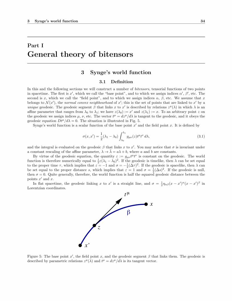
3 Synge’s world function 34
Part I
General theory of bitensors
3 Synge’s world function
3.1 Definition
In this and the following sections we will construct a number of bitensors, tensorial functions of two pointsin spacetime. The first is x′, which we call the “base point”, and to which we assign indices α′, β′, etc. Thesecond is x, which we call the “field point”, and to which we assign indices α, β, etc. We assume that xbelongs to N (x′), the normal convex neighbourhood of x′; this is the set of points that are linked to x′ by aunique geodesic. The geodesic segment β that links x to x′ is described by relations zµ(λ) in which λ is anaffine parameter that ranges from λ0 to λ1; we have z(λ0) := x′ and z(λ1) := x. To an arbitrary point z onthe geodesic we assign indices µ, ν, etc. The vector tµ = dzµ/dλ is tangent to the geodesic, and it obeys thegeodesic equation Dtµ/dλ = 0. The situation is illustrated in Fig. 5.
Synge’s world function is a scalar function of the base point x′ and the field point x. It is defined by
σ(x, x′) =1
2(λ1 − λ0)
∫ λ1
λ0
gµν(z)tµtν dλ, (3.1)
and the integral is evaluated on the geodesic β that links x to x′. You may notice that σ is invariant undera constant rescaling of the affine parameter, λ→ λ = aλ+ b, where a and b are constants.
By virtue of the geodesic equation, the quantity ε := gµνtµtν is constant on the geodesic. The world
function is therefore numerically equal to 12ε(λ1 − λ0)2. If the geodesic is timelike, then λ can be set equal
to the proper time τ , which implies that ε = −1 and σ = − 12 (∆τ)2. If the geodesic is spacelike, then λ can
be set equal to the proper distance s, which implies that ε = 1 and σ = 12 (∆s)2. If the geodesic is null,
then σ = 0. Quite generally, therefore, the world function is half the squared geodesic distance between thepoints x′ and x.
In flat spacetime, the geodesic linking x to x′ is a straight line, and σ = 12ηαβ(x − x′)α(x − x′)β in
Lorentzian coordinates.
z
tµ
x
x’
Figure 5: The base point x′, the field point x, and the geodesic segment β that links them. The geodesic isdescribed by parametric relations zµ(λ) and tµ = dzµ/dλ is its tangent vector.

3 Synge’s world function 35
3.2 Differentiation of the world function
The world function σ(x, x′) can be differentiated with respect to either argument. We let σα = ∂σ/∂xα beits partial derivative with respect to x, and σα′ = ∂σ/∂xα
′its partial derivative with respect to x′. It is
clear that σα behaves as a dual vector with respect to tensorial operations carried out at x, but as a scalarwith respect to operations carried out x′. Similarly, σα′ is a scalar at x but a dual vector at x′.
We let σαβ := ∇βσα be the covariant derivative of σα with respect to x; this is a rank-2 tensor at x anda scalar at x′. Because σ is a scalar at x, we have that this tensor is symmetric: σβα = σαβ . Similarly, we
let σαβ′ := ∂β′σα = ∂2σ/∂xβ′∂xα be the partial derivative of σα with respect to x′; this is a dual vector
both at x and x′. We can also define σα′β := ∂βσα′ = ∂2σ/∂xβ∂xα′
to be the partial derivative of σα′ withrespect to x. Because partial derivatives commute, these bitensors are equal: σβ′α = σαβ′ . Finally, we letσα′β′ := ∇β′σα′ be the covariant derivative of σα′ with respect to x′; this is a symmetric rank-2 tensor at x′
and a scalar at x.The notation is easily extended to any number of derivatives. For example, we let σαβγδ′ := ∇δ′∇γ∇β∇ασ,
which is a rank-3 tensor at x and a dual vector at x′. This bitensor is symmetric in the pair of indices αand β, but not in the pairs α and γ, nor β and γ. Because ∇δ′ is here an ordinary partial derivative withrespect to x′, the bitensor is symmetric in any pair of indices involving δ′. The ordering of the primed indexrelative to the unprimed indices is therefore irrelevant: the same bitensor can be written as σδ′αβγ or σαδ′βγor σαβδ′γ , making sure that the ordering of the unprimed indices is not altered.
More generally, we can show that derivatives of any bitensor Ω···(x, x′) satisfy the property
Ω··· ;βα′··· = Ω··· ;α′β···, (3.2)
in which “· · · ” stands for any combination of primed and unprimed indices. We start by establishing thesymmetry of Ω··· ;αβ′ with respect to the pair α and β′. This is most easily done by adopting Fermi normalcoordinates (see Sec. 9) adapted to the geodesic β and setting the connection to zero both at x and x′.In these coordinates, the bitensor Ω··· ;α is the partial derivative of Ω··· with respect to xα, and Ω··· ;αβ′ is
obtained by taking an additional partial derivative with respect to xβ′. These two operations commute, and
Ω··· ;β′α = Ω··· ;αβ′ follows as a bitensorial identity. Equation (3.2) then follows by further differentiation withrespect to either x or x′.
The message of Eq. (3.2), when applied to derivatives of the world function, is that while the orderingof the primed and unprimed indices relative to themselves is important, their ordering with respect to eachother is arbitrary. For example, σα′β′γδ′ε = σα′β′δ′γε = σγεα′β′δ′ .
3.3 Evaluation of first derivatives
We can compute σα by examining how σ varies when the field point x moves. We let the new field point bex+ δx, and δσ := σ(x+ δx, x′)−σ(x, x′) is the corresponding variation of the world function. We let β+ δβbe the unique geodesic segment that links x+ δx to x′; it is described by relations zµ(λ) + δzµ(λ), in whichthe affine parameter is scaled in such a way that it runs from λ0 to λ1 also on the new geodesic. We notethat δz(λ0) = δx′ = 0 and δz(λ1) = δx.
Working to first order in the variations, Eq. (3.1) implies
δσ = ∆λ
∫ λ1
λ0
(gµν z
µ δzν +1
2gµν,λz
µzν δzλ)dλ,
where ∆λ = λ1−λ0, an overdot indicates differentiation with respect to λ, and the metric and its derivativesare evaluated on β. Integrating the first term by parts gives
δσ = ∆λ[gµν z
µ δzν]λ1
λ0
−∆λ
∫ λ1
λ0
(gµν z
ν + Γµνλzν zλ)δzµ dλ.
The integral vanishes because zµ(λ) satisfies the geodesic equation. The boundary term at λ0 is zero becausethe variation δzµ vanishes there. We are left with δσ = ∆λgαβt
αδxβ , or
σα(x, x′) = (λ1 − λ0) gαβtβ , (3.3)

3 Synge’s world function 36
in which the metric and the tangent vector are both evaluated at x. Apart from a factor ∆λ, we see thatσα(x, x′) is equal to the geodesic’s tangent vector at x. If in Eq. (3.3) we replace x by a generic point z(λ)on β, and if we correspondingly replace λ1 by λ, we obtain σµ(z, x′) = (λ − λ0)tµ; we therefore see thatσµ(z, x′) is a rescaled tangent vector on the geodesic.
A virtually identical calculation reveals how σ varies under a change of base point x′. Here the variationof the geodesic is such that δz(λ0) = δx′ and δz(λ1) = δx = 0, and we obtain δσ = −∆λgα′β′t
α′δxβ′. This
shows thatσα′(x, x
′) = −(λ1 − λ0) gα′β′tβ′ , (3.4)
in which the metric and the tangent vector are both evaluated at x′. Apart from a factor ∆λ, we see thatσα′(x, x′) is minus the geodesic’s tangent vector at x′.It is interesting to compute the norm of σα. According to Eq. (3.3) we have gαβσ
ασβ = (∆λ)2gαβtαtβ =
(∆λ)2ε. According to Eq. (3.1), this is equal to 2σ. We have obtained
gαβσασβ = 2σ, (3.5)
and similarly,gα′β′σα′σβ′ = 2σ. (3.6)
These important relations will be the starting point of many computations to be described below.We note that in flat spacetime, σα = ηαβ(x − x′)β and σα′ = −ηαβ(x − x′)β in Lorentzian coordinates.
From this it follows that σαβ = σα′β′ = −σαβ′ = −σα′β = ηαβ , and finally, gαβσαβ = 4 = gα′β′σα′β′ .
3.4 Congruence of geodesics emanating from x′
If the base point x′ is kept fixed, σ can be considered to be an ordinary scalar function of x. According toEq. (3.5), this function is a solution to the nonlinear differential equation 1
2gαβσασβ = σ. Suppose that we
are presented with such a scalar field. What can we say about it?An additional differentiation of the defining equation reveals that the vector σα := σ;α satisfies
σα;βσβ = σα, (3.7)
which is the geodesic equation in a non-affine parameterization. The vector field is therefore tangent to acongruence of geodesics. The geodesics are timelike where σ < 0, they are spacelike where σ > 0, and theyare null where σ = 0. Here, for concreteness, we shall consider only the timelike subset of the congruence.
The vector
uα =σα
|2σ|1/2 (3.8)
is a normalized tangent vector that satisfies the geodesic equation in affine-parameter form: uα;βuβ = 0. The
parameter λ is then proper time τ . If λ∗ denotes the original parameterization of the geodesics, we havethat dλ∗/dτ = |2σ|−1/2, and we see that the original parameterization is singular at σ = 0.
In the affine parameterization, the expansion of the congruence is calculated to be
θ =θ∗
|2σ|1/2 , θ∗ := σα;α − 1, (3.9)
where θ∗ = (δV )−1(d/dλ∗)(δV ) is the expansion in the original parameterization (δV is the congruence’scross-sectional volume). While θ∗ is well behaved in the limit σ → 0 (we shall see below that θ∗ → 3), wehave that θ →∞. This means that the point x′ at which σ = 0 is a caustic of the congruence: all geodesicsemanate from this point.
These considerations, which all follow from a postulated relation 12gαβσασβ = σ, are clearly compatible
with our preceding explicit construction of the world function.
4 Coincidence limits 37
4 Coincidence limits
It is useful to determine the limiting behaviour of the bitensors σ··· as x approaches x′. We introduce thenotation [
Ω···]
= limx→x′
Ω···(x, x′) = a tensor at x′
to designate the limit of any bitensor Ω···(x, x′) as x approaches x′; this is called the coincidence limit of
the bitensor. We assume that the coincidence limit is a unique tensorial function of the base point x′,independent of the direction in which the limit is taken. In other words, if the limit is computed by lettingλ→ λ0 after evaluating Ω···(z, x
′) as a function of λ on a specified geodesic β, it is assumed that the answerdoes not depend on the choice of geodesic.
4.1 Computation of coincidence limits
From Eqs. (3.1), (3.3), and (3.4) we already have[σ]
= 0,[σα]
=[σα′]
= 0. (4.1)
Additional results are obtained by repeated differentiation of the relations (3.5) and (3.6). For example,Eq. (3.5) implies σγ = gαβσασβγ = σβσβγ , or (gβγ − σβγ)tβ = 0 after using Eq. (3.3). From the assumptionstated in the preceding paragraph, σβγ becomes independent of tβ in the limit x → x′, and we arrive at[σαβ ] = gα′β′ . By very similar calculations we obtain all other coincidence limits for the second derivativesof the world function. The results are[
σαβ]
=[σα′β′
]= gα′β′ ,
[σαβ′
]=[σα′β
]= −gα′β′ . (4.2)
From these relations we infer that [σαα] = 4, so that [θ∗] = 3, where θ∗ was defined in Eq. (3.9).To generate coincidence limits of bitensors involving primed indices, it is efficient to invoke Synge’s rule,[
σ···α′]
=[σ···];α′−[σ···α
], (4.3)
in which “· · · ” designates any combination of primed and unprimed indices; this rule will be establishedbelow. For example, according to Synge’s rule we have [σαβ′ ] = [σα];β′ − [σαβ ], and since the coincidencelimit of σα is zero, this gives us [σαβ′ ] = −[σαβ ] = −gα′β′ , as was stated in Eq. (4.2). Similarly, [σα′β′ ] =[σα′ ];β′ − [σα′β ] = −[σβα′ ] = gα′β′ . The results of Eq. (4.2) can thus all be generated from the known resultfor [σαβ ].
The coincidence limits of Eq. (4.2) were derived from the relation σα = σδασδ. We now differentiate thistwice more and obtain σαβγ = σδαβγσδ + σδαβσδγ + σδαγσδβ + σδασδβγ . At coincidence we have[
σαβγ]
=[σδαβ
]gδ′γ′ +
[σδαγ
]gδ′β′ + δδ
′
α′[σδβγ
],
or [σγαβ ] + [σβαγ ] = 0 if we recognize that the operations of raising or lowering indices and taking the limitx→ x′ commute. Noting the symmetries of σαβ , this gives us [σαγβ ]+[σαβγ ] = 0, or 2[σαβγ ]− [Rδαβγσδ] = 0,
or 2[σαβγ ] = Rδ′
α′β′γ′ [σδ′ ]. Since the last factor is zero, we arrive at[σαβγ
]=[σαβγ′
]=[σαβ′γ′
]=[σα′β′γ′
]= 0. (4.4)
The last three results were derived from [σαβγ ] = 0 by employing Synge’s rule.We now differentiate the relation σα = σδασδ three times and obtain
σαβγδ = σεαβγδσε + σεαβγσεδ + σεαβδσεγ + σεαγδσεβ + σεαβσεγδ + σεαγσεβδ + σεαδσεβγ + σεασεβγδ.
At coincidence this reduces to [σαβγδ] + [σαδβγ ] + [σαγβδ] = 0. To simplify the third term we differentiateRicci’s identity σαγβ = σαβγ −Rεαβγσε with respect to xδ and then take the coincidence limit. This gives us[σαγβδ] = [σαβγδ] +Rα′δ′β′γ′ . The same manipulations on the second term give [σαδβγ ] = [σαβδγ ] +Rα′γ′β′δ′ .Using the identity σαβδγ = σαβγδ−Rεαγδσεβ−Rεβγδσαε and the symmetries of the Riemann tensor, it is theneasy to show that [σαβδγ ] = [σαβγδ]. Gathering the results, we obtain 3[σαβγδ] + Rα′γ′β′δ′ + Rα′δ′β′γ′ = 0,

4 Coincidence limits 38
and Synge’s rule allows us to generalize this to any combination of primed and unprimed indices. Our finalresults are [
σαβγδ]
= −1
3
(Rα′γ′β′δ′ +Rα′δ′β′γ′
),
[σαβγδ′
]=
1
3
(Rα′γ′β′δ′ +Rα′δ′β′γ′
),[
σαβγ′δ′]
= −1
3
(Rα′γ′β′δ′ +Rα′δ′β′γ′
),
[σαβ′γ′δ′
]= −1
3
(Rα′β′γ′δ′ +Rα′γ′β′δ′
),[
σα′β′γ′δ′]
= −1
3
(Rα′γ′β′δ′ +Rα′δ′β′γ′
). (4.5)
4.2 Derivation of Synge’s rule
We begin with any bitensor ΩAB′(x, x′) in which A = α · · ·β is a multi-index that represents any number
of unprimed indices, and B′ = γ′ · · · δ′ a multi-index that represents any number of primed indices. (It doesnot matter whether the primed and unprimed indices are segregated or mixed.) On the geodesic β that linksx to x′ we introduce an ordinary tensor PM (z) where M is a multi-index that contains the same number ofindices as A. This tensor is arbitrary, but we assume that it is parallel transported on β; this means that itsatisfies PA;αt
α = 0 at x. Similarly, we introduce an ordinary tensor QN (z) in which N contains the samenumber of indices as B′. This tensor is arbitrary, but we assume that it is parallel transported on β; at x′
it satisfies QB′
;α′tα′ = 0. With Ω, P , and Q we form a biscalar H(x, x′) defined by
H(x, x′) = ΩAB′(x, x′)PA(x)QB
′(x′).
Having specified the geodesic that links x to x′, we can consider H to be a function of λ0 and λ1. If λ1 isnot much larger than λ0 (so that x is not far from x′), we can express H(λ1, λ0) as
H(λ1, λ0) = H(λ0, λ0) + (λ1 − λ0)∂H
∂λ1
∣∣∣∣λ1=λ0
+ · · · .
Alternatively,
H(λ1, λ0) = H(λ1, λ1)− (λ1 − λ0)∂H
∂λ0
∣∣∣∣λ0=λ1
+ · · · ,
and these two expressions give
d
dλ0H(λ0, λ0) =
∂H
∂λ0
∣∣∣∣λ0=λ1
+∂H
∂λ1
∣∣∣∣λ1=λ0
,
because the left-hand side is the limit of [H(λ1, λ1)−H(λ0, λ0)]/(λ1−λ0) when λ1 → λ0. The partial deriva-tive of H with respect to λ0 is equal to ΩAB′;α′t
α′PAQB′, and in the limit this becomes [ΩAB′;α′ ]t
α′PA′QB
′.
Similarly, the partial derivative of H with respect to λ1 is ΩAB′;αtαPAQB
′, and in the limit λ1 → λ0 this
becomes [ΩAB′;α]tα′PA
′QB
′. Finally, H(λ0, λ0) = [ΩAB′ ]P
A′QB′, and its derivative with respect to λ0 is
[ΩAB′ ];α′tα′PA
′QB
′. Gathering the results we find that[
ΩAB′];α′−[ΩAB′;α′
]−[ΩAB′;α
]tα′PA
′QB
′= 0,
and the final statement of Synge’s rule,[ΩAB′
];α′
=[ΩAB′;α′
]+[ΩAB′;α
], (4.6)
follows from the fact that the tensors PM and QN , and the direction of the selected geodesic β, are allarbitrary. Equation (4.6) reduces to Eq. (4.3) when σ··· is substituted in place of ΩAB′ .

5 Parallel propagator 39
5 Parallel propagator
5.1 Tetrad on β
On the geodesic segment β that links x to x′ we introduce an orthonormal basis eµa (z) that is paralleltransported on the geodesic. The frame indices a, b, . . . , run from 0 to 3 and the basis vectors satisfy
gµν eµa eνb = ηab,
Deµadλ
= 0, (5.1)
where ηab = diag(−1, 1, 1, 1) is the Minkowski metric (which we shall use to raise and lower frame indices).We have the completeness relations
gµν = ηab eµa eνb , (5.2)
and we define a dual tetrad eaµ(z) by
eaµ := ηabgµν eνb ; (5.3)
this is also parallel transported on β. In terms of the dual tetrad the completeness relations take the form
gµν = ηab eaµe
bν , (5.4)
and it is easy to show that the tetrad and its dual satisfy eaµeµb = δab and eaνe
µa = δµν . Equations (5.1)–(5.4)
hold everywhere on β. In particular, with an appropriate change of notation they hold at x′ and x; forexample, gαβ = ηab e
aαe
bβ is the metric at x.
(You will have noticed that we use sans-serif symbols for the frame indices. This is to distinguish themfrom another set of frame indices that will appear below. The frame indices introduced here run from 0 to3; those to be introduced later will run from 1 to 3.)
5.2 Definition and properties of the parallel propagator
Any vector field Aµ(z) on β can be decomposed in the basis eµa : Aµ = Aa eµa , and the vector’s framecomponents are given by Aa = Aµ eaµ. If Aµ is parallel transported on the geodesic, then the coefficients Aa
are constants. The vector at x can then be expressed as Aα = (Aα′eaα′)e
αa , or
Aα(x) = gαα′(x, x′)Aα
′(x′), gαα′(x, x
′) := eαa (x) eaα′(x′). (5.5)
The object gαα′ = eαa eaα′ is the parallel propagator: it takes a vector at x′ and parallel-transports it to x along
the unique geodesic that links these points.Similarly, we find that
Aα′(x′) = gα
′
α(x′, x)Aα(x), gα′
α(x′, x) := eα′
a (x′) eaα(x), (5.6)
and we see that gα′
α = eα′
a eaα performs the inverse operation: it takes a vector at x and parallel-transports it
back to x′. Clearly,gαα′g
α′
β = δαβ , gα′
αgαβ′ = δα
′
β′ , (5.7)
and these relations formally express the fact that gα′
α is the inverse of gαα′ .
The relation gαα′ = eαa eaα′ can also be expressed as g α′
α = eaαeα′
a , and this reveals that
g α′
α (x, x′) = gα′
α(x′, x), g αα′ (x
′, x) = gαα′(x, x′). (5.8)
The ordering of the indices, and the ordering of the arguments, are arbitrary.The action of the parallel propagator on tensors of arbitrary rank is easy to figure out. For example,
suppose that the dual vector pµ = pa eaµ is parallel transported on β. Then the frame components pa = pµ e
µa
are constants, and the dual vector at x can be expressed as pα = (pα′eα′
a )eαa , or
pα(x) = gα′
α(x′, x) pα′(x′). (5.9)
6 Expansion of bitensors near coincidence 40
It is therefore the inverse propagator gα′
α that takes a dual vector at x′ and parallel-transports it to x. Asanother example, it is easy to show that a tensor Aαβ at x obtained by parallel transport from x′ must begiven by
Aαβ(x) = gαα′(x, x′)gββ′(x, x
′)Aα′β′(x′). (5.10)
Here we need two occurrences of the parallel propagator, one for each tensorial index. Because the metrictensor is covariantly constant, it is automatically parallel transported on β, and a special case of Eq. (5.10)
is gαβ = gα′
αgβ′
β gα′β′ .
Because the basis vectors are parallel transported on β, they satisfy eαa;βσβ = 0 at x and eα
′
a;β′σβ′ = 0 at
x′. This immediately implies that the parallel propagators must satisfy
gαα′;βσβ = gαα′;β′σ
β′ = 0, gα′
α;βσβ = gα
′
α;β′σβ′ = 0. (5.11)
Another useful property of the parallel propagator follows from the fact that if tµ = dzµ/dλ is tangent tothe geodesic connecting x to x′, then tα = gαα′t
α′ . Using Eqs. (3.3) and (3.4), this observation gives us therelations
σα = −gα′ασα′ , σα′ = −gαα′σα. (5.12)
5.3 Coincidence limits
Equation (5.5) and the completeness relations of Eqs. (5.2) or (5.4) imply that[gαβ′
]= δα
′
β′ . (5.13)
Other coincidence limits are obtained by differentiation of Eqs. (5.11). For example, the relation gαβ′;γσγ = 0
implies gαβ′;γδσγ + gαβ′;γσ
γδ = 0, and at coincidence we have[
gαβ′;γ]
=[gαβ′;γ′
]= 0; (5.14)
the second result was obtained by applying Synge’s rule on the first result. Further differentiation gives
gαβ′;γδεσγ + gαβ′;γδσ
γε + gαβ′;γεσ
γδ + gαβ′;γσ
γδε = 0,
and at coincidence we have [gαβ′;γδ] + [gαβ′;δγ ] = 0, or 2[gαβ′;γδ] + Rα′
β′γ′δ′ = 0. The coincidence limit forgαβ′;γδ′ = gαβ′;δ′γ can then be obtained from Synge’s rule, and an additional application of the rule gives[gαβ′;γ′δ′ ]. Our results are
[gαβ′;γδ
]= −1
2Rα′
β′γ′δ′ ,[gαβ′;γδ′
]=
1
2Rα′
β′γ′δ′ ,
(5.15)[gαβ′;γ′δ
]= −1
2Rα′
β′γ′δ′ ,[gαβ′;γ′δ′
]=
1
2Rα′
β′γ′δ′ .
6 Expansion of bitensors near coincidence
6.1 General method
We would like to express a bitensor Ωα′β′(x, x′) near coincidence as an expansion in powers of −σα′(x, x′),
the closest analogue in curved spacetime to the flat-spacetime quantity (x− x′)α. For concreteness we shallconsider the case of rank-2 bitensor, and for the moment we will assume that the tensorial indices all referto the base point x′.
The expansion we seek is of the form
Ωα′β′(x, x′) = Aα′β′ +Aα′β′γ′ σ
γ′ +1
2Aα′β′γ′δ′ σ
γ′σδ′+O(ε3), (6.1)

6 Expansion of bitensors near coincidence 41
in which the “expansion coefficients” Aα′β′ , Aα′β′γ′ , and Aα′β′γ′δ′ are all ordinary tensors at x′; this last
tensor is symmetric in the pair of indices γ′ and δ′, and ε measures the size of a typical component of σα′.
To find the expansion coefficients we differentiate Eq. (6.1) repeatedly and take coincidence limits. Equa-tion (6.1) immediately implies [Ωα′β′ ] = Aα′β′ . After one differentiation we obtain Ωα′β′;γ′ = Aα′β′;γ′ +
Aα′β′ε′;γ′σε′ + Aα′β′ε′σ
ε′
γ′ + 12 Aα′β′ε′ι′;γ′σ
ε′σι′+ Aα′β′ε′ι′σ
ε′σι′
γ′ + O(ε2), and at coincidence this reduces to[Ωα′β′;γ′ ] = Aα′β′;γ′ + Aα′β′γ′ . Taking the coincidence limit after two differentiations yields [Ωα′β′;γ′δ′ ] =Aα′β′;γ′δ′ +Aα′β′γ′;δ′ +Aα′β′δ′;γ′ +Aα′β′γ′δ′ . The expansion coefficients are therefore
Aα′β′ =[Ωα′β′
],
Aα′β′γ′ =[Ωα′β′;γ′
]−Aα′β′;γ′ ,
Aα′β′γ′δ′ =[Ωα′β′;γ′δ′
]−Aα′β′;γ′δ′ −Aα′β′γ′;δ′ −Aα′β′δ′;γ′ . (6.2)
These results are to be substituted into Eq. (6.1), and this gives us Ωα′β′(x, x′) to second order in ε.
Suppose now that the bitensor is Ωα′β , with one index referring to x′ and the other to x. The previous
procedure can be applied directly if we introduce an auxiliary bitensor Ωα′β′ := gββ′Ωα′β whose indices all
refer to the point x′. Then Ωα′β′ can be expanded as in Eq. (6.1), and the original bitensor is reconstructed
as Ωα′β = gβ′
βΩα′β′ , or
Ωα′β(x, x′) = gβ′
β
(Bα′β′ +Bα′β′γ′ σ
γ′ +1
2Bα′β′γ′δ′ σ
γ′σδ′)
+O(ε3). (6.3)
The expansion coefficients can be obtained from the coincidence limits of Ωα′β′ and its derivatives. It isconvenient, however, to express them directly in terms of the original bitensor Ωα′β by substituting the
relation Ωα′β′ = gββ′Ωα′β and its derivatives. After using the results of Eq. (5.13)–(5.15) we find
Bα′β′ =[Ωα′β
],
Bα′β′γ′ =[Ωα′β;γ′
]−Bα′β′;γ′ ,
Bα′β′γ′δ′ =[Ωα′β;γ′δ′
]+
1
2Bα′ε′R
ε′
β′γ′δ′ −Bα′β′;γ′δ′ −Bα′β′γ′;δ′ −Bα′β′δ′;γ′ . (6.4)
The only difference with respect to Eq. (6.3) is the presence of a Riemann-tensor term in Bα′β′γ′δ′ .Suppose finally that the bitensor to be expanded is Ωαβ , whose indices all refer to x. Much as we did
before, we introduce an auxiliary bitensor Ωα′β′ = gαα′gββ′Ωαβ whose indices all refer to x′, we expand Ωα′β′
as in Eq. (6.1), and we then reconstruct the original bitensor. This gives us
Ωαβ(x, x′) = gα′
αgβ′
β
(Cα′β′ + Cα′β′γ′ σ
γ′ +1
2Cα′β′γ′δ′ σ
γ′σδ′)
+O(ε3), (6.5)
and the expansion coefficients are now
Cα′β′ =[Ωαβ
],
Cα′β′γ′ =[Ωαβ;γ′
]− Cα′β′;γ′ ,
Cα′β′γ′δ′ =[Ωαβ;γ′δ′
]+
1
2Cα′ε′R
ε′
β′γ′δ′ +1
2Cε′β′R
ε′
α′γ′δ′ − Cα′β′;γ′δ′ − Cα′β′γ′;δ′ − Cα′β′δ′;γ′ . (6.6)
This differs from Eq. (6.4) by the presence of an additional Riemann-tensor term in Cα′β′γ′δ′ .
6.2 Special cases
We now apply the general expansion method developed in the preceding subsection to the bitensors σα′β′ ,σα′β , and σαβ . In the first instance we have Aα′β′ = gα′β′ , Aα′β′γ′ = 0, and Aα′β′γ′δ′ = − 1
3 (Rα′γ′β′δ′ +Rα′δ′β′γ′). In the second instance we have Bα′β′ = −gα′β′ , Bα′β′γ′ = 0, and Bα′β′γ′δ′ = − 1
3 (Rβ′α′γ′δ′ +

7 van Vleck determinant 42
Rβ′γ′α′δ′)− 12Rα′β′γ′δ′ = − 1
3Rα′δ′β′γ′ − 16Rα′β′γ′δ′ . In the third instance we have Cα′β′ = gα′β′ , Cα′β′γ′ = 0,
and Cα′β′γ′δ′ = − 13 (Rα′γ′β′δ′ +Rα′δ′β′γ′). This gives us the expansions
σα′β′ = gα′β′ −1
3Rα′γ′β′δ′ σ
γ′σδ′+O(ε3), (6.7)
σα′β = −gβ′
β
(gα′β′ +
1
6Rα′γ′β′δ′ σ
γ′σδ′)
+O(ε3), (6.8)
σαβ = gα′
αgβ′
β′
(gα′β′ −
1
3Rα′γ′β′δ′ σ
γ′σδ′)
+O(ε3). (6.9)
Taking the trace of the last equation returns σαα = 4− 13Rγ′δ′ σ
γ′σδ′+O(ε3), or
θ∗ = 3− 1
3Rα′β′ σ
α′σβ′+O(ε3), (6.10)
where θ∗ := σαα − 1 was shown in Sec. 3.4 to describe the expansion of the congruence of geodesics thatemanate from x′. Equation (6.10) reveals that timelike geodesics are focused if the Ricci tensor is nonzeroand the strong energy condition holds: when Rα′β′ σ
α′σβ′> 0 we see that θ∗ is smaller than 3, the value it
would take in flat spacetime.The expansion method can easily be extended to bitensors of other tensorial ranks. In particular, it can
be adapted to give expansions of the first derivatives of the parallel propagator. The expansions
gαβ′;γ′ =1
2gαα′R
α′
β′γ′δ′ σδ′ +O(ε2), gαβ′;γ =
1
2gαα′g
γ′
γRα′
β′γ′δ′ σδ′ +O(ε2) (6.11)
and thus easy to establish, and they will be needed in part III of this review.
6.3 Expansion of tensors
The expansion method can also be applied to ordinary tensor fields. For concreteness, suppose that we wishto express a rank-2 tensor Aαβ at a point x in terms of its values (and that of its covariant derivatives) at a
neighbouring point x′. The tensor can be written as an expansion in powers of −σα′(x, x′) and in this casewe have
Aαβ(x) = gα′
αgβ′
β
(Aα′β′ −Aα′β′;γ′ σγ
′+
1
2Aα′β′;γ′δ′ σ
γ′σδ′)
+O(ε3). (6.12)
If the tensor field is parallel transported on the geodesic β that links x to x′, then Eq. (6.12) reduces toEq. (5.10). The extension of this formula to tensors of other ranks is obvious.
To derive this result we express Aµν(z), the restriction of the tensor field on β, in terms of its tetrad com-ponents Aab(λ) = Aµνe
µa eνb . Recall from Sec. 5.1 that eµa is an orthonormal basis that is parallel transported
on β; recall also that the affine parameter λ ranges from λ0 (its value at x′) to λ1 (its value at x). We haveAα′β′(x
′) = Aab(λ0)eaα′ebβ′ , Aαβ(x) = Aab(λ1)eaαe
bβ , and Aab(λ1) can be expressed in terms of quantities at
λ = λ0 by straightforward Taylor expansion. Since, for example,
(λ1 − λ0)dAab
dλ
∣∣∣∣λ0
= (λ1 − λ0)(Aµνe
µa eνb
);λtλ∣∣∣λ0
= (λ1 − λ0)Aµν;λeµa eνb tλ∣∣∣λ0
= −Aα′β′;γ′eα′
a eβ′
b σγ′ ,
where we have used Eq. (3.4), we arrive at Eq. (6.12) after involving Eq. (5.6).
7 van Vleck determinant
7.1 Definition and properties
The van Vleck biscalar ∆(x, x′) is defined by
∆(x, x′) := det[∆α′
β′(x, x′)], ∆α′
β′(x, x′) := −gα′α(x′, x)σαβ′(x, x
′). (7.1)

7 van Vleck determinant 43
As we shall show below, it can also be expressed as
∆(x, x′) = −det[−σαβ′(x, x′)
]√−g√−g′ , (7.2)
where g is the metric determinant at x and g′ the metric determinant at x′.Equations (4.2) and (5.13) imply that at coincidence, [∆α′
β′ ] = δα′
β′ and [∆] = 1. Equation (6.8), on theother hand, implies that near coincidence,
∆α′
β′ = δα′
β′ +1
6Rα′
γ′β′δ′ σγ′σδ
′+O(ε3), (7.3)
so that
∆ = 1 +1
6Rα′β′ σ
α′σβ′+O(ε3). (7.4)
This last result follows from the fact that for a “small” matrix a, det(1 + a) = 1 + tr(a) +O(a2).We shall prove below that the van Vleck determinant satisfies the differential equation
1
∆
(∆σα
);α
= 4, (7.5)
which can also be written as (ln ∆),ασα = 4− σαα, or
d
dλ∗(ln ∆) = 3− θ∗ (7.6)
in the notation introduced in Sec. 3.4. Equation (7.6) reveals that the behaviour of the van Vleck determinantis governed by the expansion of the congruence of geodesics that emanate from x′. If θ∗ < 3, then thecongruence expands less rapidly than it would in flat spacetime, and ∆ increases along the geodesics. If, onthe other hand, θ∗ > 3, then the congruence expands more rapidly than it would in flat spacetime, and ∆decreases along the geodesics. Thus, ∆ > 1 indicates that the geodesics are undergoing focusing, while ∆ < 1indicates that the geodesics are undergoing defocusing. The connection between the van Vleck determinantand the strong energy condition is well illustrated by Eq. (7.4): the sign of ∆− 1 near x′ is determined bythe sign of Rα′β′ σ
α′σβ′.
7.2 Derivations
To show that Eq. (7.2) follows from Eq. (7.1) we rewrite the completeness relations at x, gαβ = ηabeαa eβb ,
in the matrix form g−1 = EηET , where E denotes the 4 × 4 matrix whose entries correspond to eαa . (Inthis translation we put tensor and frame indices on an equal footing.) With e denoting the determinantof this matrix, we have 1/g = −e2, or e = 1/
√−g. Similarly, we rewrite the completeness relations at x′,
gα′β′ = ηabeα
′
a eβ′
b , in the matrix form g′−1 = E′ηE′T , where E′ is the matrix corresponding to eα′
a . Withe′ denoting its determinant, we have 1/g′ = −e′2, or e′ = 1/
√−g′. Now, the parallel propagator is defined
by gαα′ = ηabgα′β′eαa eβ′
b , and the matrix form of this equation is g = EηE′Tg′T . The determinant of theparallel propagator is therefore g = −ee′g′ =
√−g′/√−g. So we have
det[gαα′
]=
√−g′√−g , det[gα′
α
]=
√−g√−g′ , (7.7)
and Eq. (7.2) follows from the fact that the matrix form of Eq. (7.1) is ∆ = −g−1g−1σ, where σ is thematrix corresponding to σαβ′ .
To establish Eq. (7.5) we differentiate the relation σ = 12σ
γσγ twice and obtain σαβ′ = σγασγβ′+σγσγαβ′ .
If we replace the last factor by σαβ′γ and multiply both sides by −gα′α we find
∆α′
β′ = −gα′α(σγασγβ′ + σγσαβ′γ
).

7 van Vleck determinant 44
In this expression we make the substitution σαβ′ = −gαα′∆α′
β′ , which follows directly from Eq. (7.1). Thisgives us
∆α′
β′ = gα′
αgγγ′σ
αγ∆γ′
β′ + ∆α′
β′;γσγ , (7.8)
where we have used Eq. (5.11). At this stage we introduce an inverse (∆−1)α′
β′ to the van Vleck bitensor,
defined by ∆α′
β′(∆−1)β
′
γ′ = δα′
γ′ . After multiplying both sides of Eq. (7.8) by (∆−1)β′
γ′ we find
δα′
β′ = gα′
αgββ′σ
αβ + (∆−1)γ
′
β′∆α′
γ′;γσγ ,
and taking the trace of this equation yields
4 = σαα + (∆−1)β′
α′∆α′
β′;γσγ .
We now recall the identity δ ln detM = Tr(M−1δM), which relates the variation of a determinant to the
variation of the matrix elements. It implies, in particular, that (∆−1)β′
α′∆α′
β′;γ = (ln ∆),γ , and we finallyobtain
4 = σαα + (ln ∆),ασα, (7.9)
which is equivalent to Eq. (7.5) or Eq. (7.6).

8 Riemann normal coordinates 45
Part II
Coordinate systems
8 Riemann normal coordinates
8.1 Definition and coordinate transformation
Given a fixed base point x′ and a tetrad eα′
a (x′), we assign to a neighbouring point x the four coordinates
xa = −eaα′(x′)σα′(x, x′), (8.1)
where eaα′ = ηabgα′β′eβ′
b is the dual tetrad attached to x′. The new coordinates xa are called Riemann normal
coordinates (RNC), and they are such that ηabxaxb = ηabe
aα′e
bβ′σ
α′σβ′
= gα′β′σα′σβ
′, or
ηabxaxb = 2σ(x, x′). (8.2)
Thus, ηabxaxb is the squared geodesic distance between x and the base point x′. It is obvious that x′ is at
the origin of the RNC, where xa = 0.If we move the point x to x + δx, the new coordinates change to xa + δxa = −eaα′σα
′(x + δx, x′) =
xa − eaα′σα′
β δxβ , so that
dxa = −eaα′σα′
β dxβ . (8.3)
The coordinate transformation is therefore determined by ∂xa/∂xβ = −eaα′σα′
β , and at coincidence we have[∂xa
∂xα
]= eaα′ ,
[∂xα
∂xa
]= eα
′
a ; (8.4)
the second result follows from the identities eaα′eα′
b = δab and eα′
a eaβ′ = δα
′
β′ .
It is interesting to note that the Jacobian of the transformation of Eq. (8.3), J := det(∂xa/∂xβ), is givenby J =
√−g∆(x, x′), where g is the determinant of the metric in the original coordinates, and ∆(x, x′) isthe Van Vleck determinant of Eq. (7.2). This result follows simply by writing the coordinate transformationin the form ∂xa/∂xβ = −ηabeα′b σα′β and computing the product of the determinants. It allows us to deducethat in RNC, the determinant of the metric is given by√
−g(RNC) =1
∆(x, x′). (8.5)
It is easy to show that the geodesics emanating from x′ are straight coordinate lines in RNC. The propervolume of a small comoving region is then equal to dV = ∆−1 d4x, and this is smaller than the flat-spacetimevalue of d4x if ∆ > 1, that is, if the geodesics are focused by the spacetime curvature.
8.2 Metric near x′
We now would like to invert Eq. (8.3) in order to express the line element ds2 = gαβ dxαdxβ in terms of the
displacements dxa. We shall do this approximately, by working in a small neighbourhood of x′. We recallthe expansion of Eq. (6.8),
σα′
β = −gβ′
β
(δα′
β′ +1
6Rα′
γ′β′δ′σγ′σδ
′)
+O(ε3),
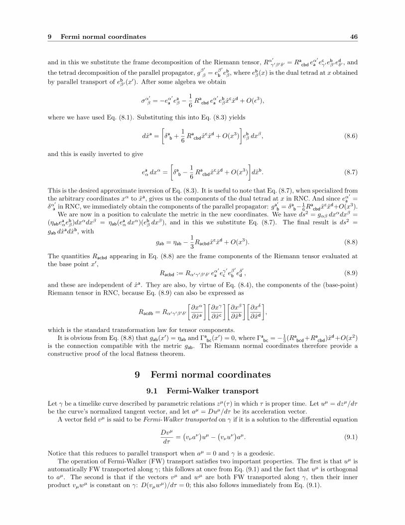
9 Fermi normal coordinates 46
and in this we substitute the frame decomposition of the Riemann tensor, Rα′
γ′β′δ′ = Racbd e
α′
a ecγ′e
bβ′e
dδ′ , and
the tetrad decomposition of the parallel propagator, gβ′
β = eβ′
b ebβ , where ebβ(x) is the dual tetrad at x obtained
by parallel transport of ebβ′(x′). After some algebra we obtain
σα′
β = −eα′a eaβ −1
6Ra
cbd eα′
a ebβ x
cxd +O(ε3),
where we have used Eq. (8.1). Substituting this into Eq. (8.3) yields
dxa =
[δab +
1
6Ra
cbdxcxd +O(x3)
]ebβ dx
β , (8.6)
and this is easily inverted to give
eaα dxα =
[δab −
1
6Ra
cbdxcxd +O(x3)
]dxb. (8.7)
This is the desired approximate inversion of Eq. (8.3). It is useful to note that Eq. (8.7), when specialized fromthe arbitrary coordinates xα to xa, gives us the components of the dual tetrad at x in RNC. And since eα
′
a =δα′
a in RNC, we immediately obtain the components of the parallel propagator: ga′
b = δab− 16R
acbdx
cxd+O(x3).We are now in a position to calculate the metric in the new coordinates. We have ds2 = gαβ dx
αdxβ =(ηabe
aαe
bβ)dxαdxβ = ηab(e
aα dx
α)(ebβ dxβ), and in this we substitute Eq. (8.7). The final result is ds2 =
gab dxadxb, with
gab = ηab −1
3Racbdx
cxd +O(x3). (8.8)
The quantities Racbd appearing in Eq. (8.8) are the frame components of the Riemann tensor evaluated atthe base point x′,
Racbd := Rα′γ′β′δ′ eα′
a eγ′
c eβ′
b eδ′
d , (8.9)
and these are independent of xa. They are also, by virtue of Eq. (8.4), the components of the (base-point)Riemann tensor in RNC, because Eq. (8.9) can also be expressed as
Racdb = Rα′γ′β′δ′
[∂xα
∂xa
][∂xγ
∂xc
][∂xβ
∂xb
][∂xδ
∂xd
],
which is the standard transformation law for tensor components.It is obvious from Eq. (8.8) that gab(x
′) = ηab and Γabc(x
′) = 0, where Γabc = − 1
3 (Rabcd+Ra
cbd)xd+O(x2)
is the connection compatible with the metric gab. The Riemann normal coordinates therefore provide aconstructive proof of the local flatness theorem.
9 Fermi normal coordinates
9.1 Fermi-Walker transport
Let γ be a timelike curve described by parametric relations zµ(τ) in which τ is proper time. Let uµ = dzµ/dτbe the curve’s normalized tangent vector, and let aµ = Duµ/dτ be its acceleration vector.
A vector field vµ is said to be Fermi-Walker transported on γ if it is a solution to the differential equation
Dvµ
dτ=(vνa
ν)uµ −
(vνu
ν)aµ. (9.1)
Notice that this reduces to parallel transport when aµ = 0 and γ is a geodesic.The operation of Fermi-Walker (FW) transport satisfies two important properties. The first is that uµ is
automatically FW transported along γ; this follows at once from Eq. (9.1) and the fact that uµ is orthogonalto aµ. The second is that if the vectors vµ and wµ are both FW transported along γ, then their innerproduct vµw
µ is constant on γ: D(vµwµ)/dτ = 0; this also follows immediately from Eq. (9.1).
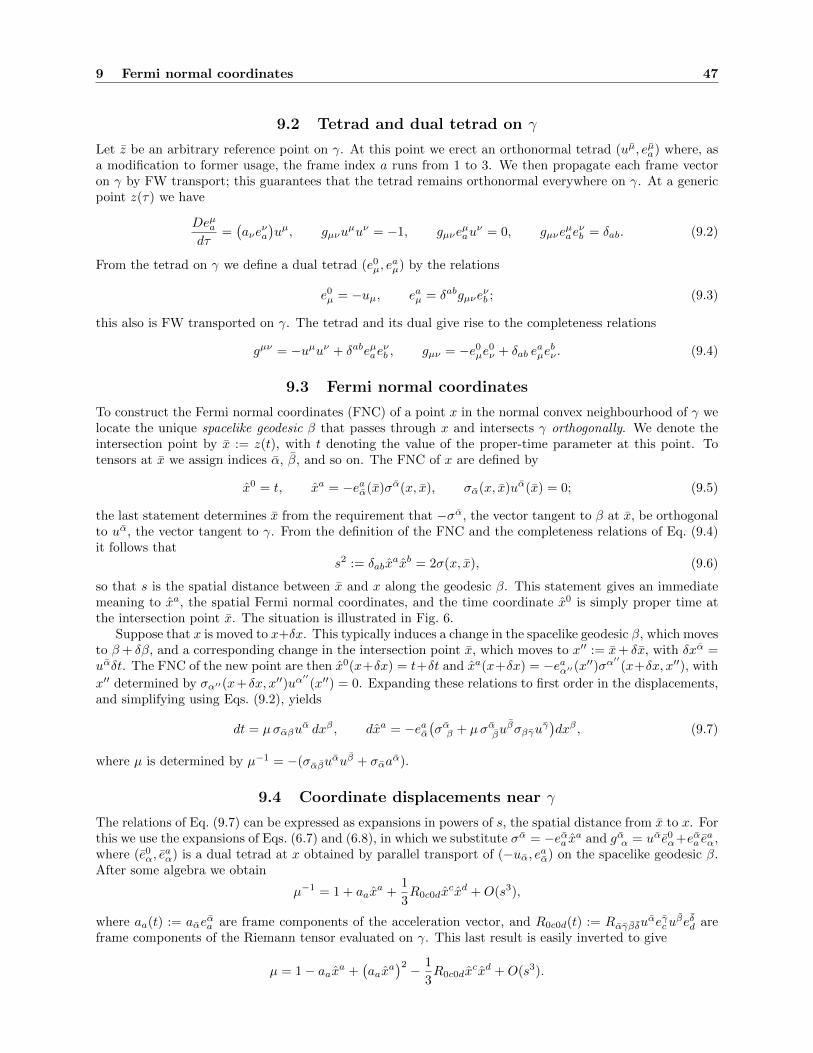
9 Fermi normal coordinates 47
9.2 Tetrad and dual tetrad on γ
Let z be an arbitrary reference point on γ. At this point we erect an orthonormal tetrad (uµ, eµa) where, asa modification to former usage, the frame index a runs from 1 to 3. We then propagate each frame vectoron γ by FW transport; this guarantees that the tetrad remains orthonormal everywhere on γ. At a genericpoint z(τ) we have
Deµadτ
=(aνe
νa
)uµ, gµνu
µuν = −1, gµνeµau
ν = 0, gµνeµaeνb = δab. (9.2)
From the tetrad on γ we define a dual tetrad (e0µ, e
aµ) by the relations
e0µ = −uµ, eaµ = δabgµνe
νb ; (9.3)
this also is FW transported on γ. The tetrad and its dual give rise to the completeness relations
gµν = −uµuν + δabeµaeνb , gµν = −e0
µe0ν + δab e
aµebν . (9.4)
9.3 Fermi normal coordinates
To construct the Fermi normal coordinates (FNC) of a point x in the normal convex neighbourhood of γ welocate the unique spacelike geodesic β that passes through x and intersects γ orthogonally. We denote theintersection point by x := z(t), with t denoting the value of the proper-time parameter at this point. Totensors at x we assign indices α, β, and so on. The FNC of x are defined by
x0 = t, xa = −eaα(x)σα(x, x), σα(x, x)uα(x) = 0; (9.5)
the last statement determines x from the requirement that −σα, the vector tangent to β at x, be orthogonalto uα, the vector tangent to γ. From the definition of the FNC and the completeness relations of Eq. (9.4)it follows that
s2 := δabxaxb = 2σ(x, x), (9.6)
so that s is the spatial distance between x and x along the geodesic β. This statement gives an immediatemeaning to xa, the spatial Fermi normal coordinates, and the time coordinate x0 is simply proper time atthe intersection point x. The situation is illustrated in Fig. 6.
Suppose that x is moved to x+δx. This typically induces a change in the spacelike geodesic β, which movesto β+ δβ, and a corresponding change in the intersection point x, which moves to x′′ := x+ δx, with δxα =uαδt. The FNC of the new point are then x0(x+δx) = t+δt and xa(x+δx) = −eaα′′(x′′)σα
′′(x+δx, x′′), with
x′′ determined by σα′′(x+ δx, x′′)uα′′(x′′) = 0. Expanding these relations to first order in the displacements,
and simplifying using Eqs. (9.2), yields
dt = µσαβuα dxβ , dxa = −eaα
(σαβ + µσαβu
βσβγuγ)dxβ , (9.7)
where µ is determined by µ−1 = −(σαβuαuβ + σαa
α).
9.4 Coordinate displacements near γ
The relations of Eq. (9.7) can be expressed as expansions in powers of s, the spatial distance from x to x. Forthis we use the expansions of Eqs. (6.7) and (6.8), in which we substitute σα = −eαa xa and gαα = uαe0
α+eαa eaα,
where (e0α, e
aα) is a dual tetrad at x obtained by parallel transport of (−uα, eaα) on the spacelike geodesic β.
After some algebra we obtain
µ−1 = 1 + aaxa +
1
3R0c0dx
cxd +O(s3),
where aa(t) := aαeαa are frame components of the acceleration vector, and R0c0d(t) := Rαγβδu
αeγcuβeδd are
frame components of the Riemann tensor evaluated on γ. This last result is easily inverted to give
µ = 1− aaxa +(aax
a)2 − 1
3R0c0dx
cxd +O(s3).
9 Fermi normal coordinates 48
a
xsz(t)
Figure 6: Fermi normal coordinates of a point x relative to a world line γ. The time coordinate t selectsa particular point on the word line, and the disk represents the set of spacelike geodesics that intersect γorthogonally at z(t). The unit vector ωa := xa/s selects a particular geodesic among this set, and the spatialdistance s selects a particular point on this geodesic.
Proceeding similarly for the other relations of Eq. (9.7), we obtain
dt =
[1− aaxa +
(aax
a)2 − 1
2R0c0dx
cxd +O(s3)
](e0βdx
β)
+
[−1
6R0cbdx
cxd +O(s3)
](ebβdx
β)
(9.8)
and
dxa =
[1
2Rac0dx
cxd +O(s3)
](e0βdx
β)
+
[δab +
1
6Racbdx
cxd +O(s3)
](ebβdx
β), (9.9)
where Rac0d(t) := Rαγβδeαaeγcu
βeδd and Racbd(t) := Rαγβδeαaeγc eβb eδd are additional frame components of the
Riemann tensor evaluated on γ. (Note that frame indices are raised with δab.)As a special case of Eqs. (9.8) and (9.9) we find that
∂t
∂xα
∣∣∣∣γ
= −uα,∂xa
∂xα
∣∣∣∣γ
= eaα, (9.10)
because in the limit x → x, the dual tetrad (e0α, e
aα) at x coincides with the dual tetrad (−uα, eaα) at x. It
follows that on γ, the transformation matrix between the original coordinates xα and the FNC (t, xa) isformed by the Fermi-Walker transported tetrad:
∂xα
∂t
∣∣∣∣γ
= uα,∂xα
∂xa
∣∣∣∣γ
= eαa . (9.11)
This implies that the frame components of the acceleration vector, aa(t), are also the components of theacceleration vector in FNC; orthogonality between uα and aα means that a0 = 0. Similarly, R0c0d(t), R0cbd(t),and Racbd(t) are the components of the Riemann tensor (evaluated on γ) in Fermi normal coordinates.
9.5 Metric near γ
Inversion of Eqs. (9.8) and (9.9) gives
e0αdx
α =
[1 + aax
a +1
2R0c0dx
cxd +O(s3)
]dt+
[1
6R0cbdx
cxd +O(s3)
]dxb (9.12)

9 Fermi normal coordinates 49
and
eaαdxα =
[δab −
1
6Racbdx
cxd +O(s3)
]dxb +
[−1
2Rac0dx
cxd +O(s3)
]dt. (9.13)
These relations, when specialized to the FNC, give the components of the dual tetrad at x. They can alsobe used to compute the metric at x, after invoking the completeness relations gαβ = −e0
αe0β + δabe
aαebβ . This
gives
gtt = −[1 + 2aax
a +(aax
a)2
+R0c0dxcxd +O(s3)
], (9.14)
gta = −2
3R0cadx
cxd +O(s3), (9.15)
gab = δab −1
3Racbdx
cxd +O(s3). (9.16)
This is the metric near γ in the Fermi normal coordinates. Recall that aa(t) are the components of theacceleration vector of γ — the timelike curve described by xa = 0 — while R0c0d(t), R0cbd(t), and Racbd(t)are the components of the Riemann tensor evaluated on γ.
Notice that on γ, the metric of Eqs. (9.14)–(9.16) reduces to gtt = −1 and gab = δab. On the other hand,the nonvanishing Christoffel symbols (on γ) are Γtta = Γatt = aa; these are zero (and the FNC enforce localflatness on the entire curve) when γ is a geodesic.
9.6 Thorne-Hartle-Zhang coordinates
The form of the metric can be simplified when the Ricci tensor vanishes on the world line:
Rµν(z) = 0. (9.17)
In such circumstances, a transformation from the Fermi normal coordinates (t, xa) to the Thorne-Hartle-Zhang (THZ) coordinates (t, ya) brings the metric to the form
gtt = −[1 + 2aay
a +(aay
a)2
+R0c0dycyd +O(s3)
], (9.18)
gta = −2
3R0cady
cyd +O(s3), (9.19)
gab = δab(1−R0c0dy
cyd)
+O(s3). (9.20)
We see that the transformation leaves gtt and gta unchanged, but that it diagonalizes gab. This metric wasfirst displayed in Ref. [138] and the coordinate transformation was later produced by Zhang [139].
The key to the simplification comes from Eq. (9.17), which dramatically reduces the number of inde-pendent components of the Riemann tensor. In particular, Eq. (9.17) implies that the frame componentsRacbd of the Riemann tensor are completely determined by Eab := R0a0b, which in this special case is asymmetric-tracefree tensor. To prove this we invoke the completeness relations of Eq. (9.4) and take framecomponents of Eq. (9.17). This produces the three independent equations
δcdRacbd = Eab, δcdR0cad = 0, δcdEcd = 0,
the last of which stating that Eab has a vanishing trace. Taking the trace of the first equation givesδabδcdRacbd = 0, and this implies that Racbd has five independent components. Since this is also the numberof independent components of Eab, we see that the first equation can be inverted — Racbd can be expressedin terms of Eab. A complete listing of the relevant relations is R1212 = E11 + E22 = −E33, R1213 = E23,R1223 = −E13, R1313 = E11 +E33 = −E22, R1323 = E12, and R2323 = E22 +E33 = −E11. These are summarizedby
Racbd = δabEcd + δcdEab − δadEbc − δbcEad, (9.21)
and Eab := R0a0b satisfies δabEab = 0.We may also note that the relation δcdR0cad = 0, together with the usual symmetries of the Riemann
tensor, imply that R0cad too possesses five independent components. These may thus be related to another

10 Retarded coordinates 50
symmetric-tracefree tensor Bab. We take the independent components to be R0112 := −B13, R0113 := B12,R0123 := −B11, R0212 := −B23, and R0213 := B22, and it is easy to see that all other components can beexpressed in terms of these. For example, R0223 = −R0113 = −B12, R0312 = −R0123 +R0213 = B11 + B22 =−B33, R0313 = −R0212 = B23, and R0323 = R0112 = −B13. These relations are summarized by
R0abc = −εbcdBda, (9.22)
where εabc is the three-dimensional permutation symbol. The inverse relation is Bab = − 12εacdR0bcd.
Substitution of Eq. (9.21) into Eq. (9.16) gives
gab = δab
(1− 1
3Ecdxcxd
)− 1
3
(xcx
c)Eab +
1
3xaEbcxc +
1
3xbEacxc +O(s3),
and we have not yet achieved the simple form of Eq. (9.20). The missing step is the transformation fromthe FNC xa to the THZ coordinates ya. This is given by
ya = xa + ξa, ξa = −1
6
(xcx
c)Eabxb +
1
3xaEbcxbxc +O(s4). (9.23)
It is easy to see that this transformation does not affect gtt nor gta at orders s and s2. The remainingcomponents of the metric, however, transform according to gab(THZ) = gab(FNC)− ξa;b − ξb;a, where
ξa;b =1
3δabEcdxcxd −
1
6
(xcx
c)Eab −
1
3Eacxcxb +
2
3xaEbcxc +O(s3).
It follows that gTHZab = δab(1− Ecdycyd) +O(y3), which is just the same statement as in Eq. (9.20).
Alternative expressions for the components of the THZ metric are
gtt = −[1 + 2aay
a +(aay
a)2
+ Eabyayb +O(s3)], (9.24)
gta = −2
3εabcBbdycyd +O(s3), (9.25)
gab = δab(1− Ecdycyd
)+O(s3). (9.26)
10 Retarded coordinates
10.1 Geometrical elements
We introduce the same geometrical elements as in Sec. 9: we have a timelike curve γ described by relationszµ(τ), its normalized tangent vector uµ = dzµ/dτ , and its acceleration vector aµ = Duµ/dτ . We also havean orthonormal triad eµa that is FW transported on the world line according to
Deµadτ
= aauµ, (10.1)
where aa(τ) = aµeµa are the frame components of the acceleration vector. Finally, we have a dual tetrad
(e0µ, e
aµ), with e0
µ = −uµ and eaµ = δabgµνeνb . The tetrad and its dual give rise to the completeness relations
gµν = −uµuν + δabeµaeνb , gµν = −e0
µe0ν + δab e
aµebν , (10.2)
which are the same as in Eq. (9.4).The Fermi normal coordinates of Sec. 9 were constructed on the basis of a spacelike geodesic connecting
a field point x to the world line. The retarded coordinates are based instead on a null geodesic going fromthe world line to the field point. We thus let x be within the normal convex neighbourhood of γ, β be theunique future-directed null geodesic that goes from the world line to x, and x′ := z(u) be the point at whichβ intersects the world line, with u denoting the value of the proper-time parameter at this point.

10 Retarded coordinates 51
From the tetrad at x′ we obtain another tetrad (eα0 , eαa ) at x by parallel transport on β. By raising
the frame index and lowering the vectorial index we also obtain a dual tetrad at x: e0α = −gαβeβ0 and
eaα = δabgαβeβb . The metric at x can be then be expressed as
gαβ = −e0αe
0β + δabe
aαebβ , (10.3)
and the parallel propagator from x′ to x is given by
gαα′(x, x′) = −eα0uα′ + eαae
aα′ , gα
′
α(x′, x) = uα′e0α + eα
′
a eaα. (10.4)
10.2 Definition of the retarded coordinates
The quasi-Cartesian version of the retarded coordinates are defined by
x0 = u, xa = −eaα′(x′)σα′(x, x′), σ(x, x′) = 0; (10.5)
the last statement indicates that x′ and x are linked by a null geodesic. From the fact that σα′
is a nullvector we obtain
r := (δabxaxb)1/2 = uα′σ
α′ , (10.6)
and r is a positive quantity by virtue of the fact that β is a future-directed null geodesic — this makes σα′
past-directed. In flat spacetime, σα′
= −(x − x′)α, and in a Lorentz frame that is momentarily comovingwith the world line, r = t − t′ > 0; with the speed of light set equal to unity, r is also the spatial distancebetween x′ and x as measured in this frame. In curved spacetime, the quantity r = uα′σ
α′ can still be calledthe retarded distance between the point x and the world line. Another consequence of Eq. (10.5) is that
σα′
= −r(uα′+ Ωaeα
′
a
), (10.7)
where Ωa := xa/r is a unit spatial vector that satisfies δabΩaΩb = 1.
A straightforward calculation reveals that under a displacement of the point x, the retarded coordinateschange according to
du = −kα dxα, dxa = −(raa − ωabxb + eaα′σ
α′
β′uβ′)du− eaα′σα
′
β dxβ , (10.8)
where kα = σα/r is a future-directed null vector at x that is tangent to the geodesic β. To obtain theseresults we must keep in mind that a displacement of x typically induces a simultaneous displacement ofx′ because the new points x + δx and x′ + δx′ must also be linked by a null geodesic. We therefore have0 = σ(x+ δx, x′ + δx′) = σα δx
α + σα′ δxα′ , and the first relation of Eq. (10.8) follows from the fact that a
displacement along the world line is described by δxα′
= uα′δu.
10.3 The scalar field r(x) and the vector field kα(x)
If we keep x′ linked to x by the relation σ(x, x′) = 0, then the quantity
r(x) = σα′(x, x′)uα
′(x′) (10.9)
can be viewed as an ordinary scalar field defined in a neighbourhood of γ. We can compute the gradient of rby finding how r changes under a displacement of x (which again induces a displacement of x′). The resultis
∂βr = −(σα′a
α′ + σα′β′uα′uβ
′)kβ + σα′βu
α′ . (10.10)
Similarly, we can view
kα(x) =σα(x, x′)
r(x)(10.11)
as an ordinary vector field, which is tangent to the congruence of null geodesics that emanate from x′. It iseasy to check that this vector satisfies the identities
σαβkβ = kα, σα′βk
β =σα′
r, (10.12)
10 Retarded coordinates 52
from which we also obtain σα′βuα′kβ = 1. From this last result and Eq. (10.10) we deduce the important
relationkα∂αr = 1. (10.13)
In addition, combining the general statement σα = −gαα′σα′
— cf. Eq. (5.12) — with Eq. (10.7) gives
kα = gαα′(uα′+ Ωaeα
′
a
); (10.14)
the vector at x is therefore obtained by parallel transport of uα′+ Ωaeα
′
a on β. From this and Eq. (10.4) weget the alternative expression
kα = eα0 + Ωaeαa , (10.15)
which confirms that kα is a future-directed null vector field (recall that Ωa = xa/r is a unit vector).The covariant derivative of kα can be computed by finding how the vector changes under a displacement
of x. (It is in fact easier to calculate first how rkα changes, and then substitute our previous expression for∂βr.) The result is
rkα;β = σαβ − kασβγ′uγ′ − kβσαγ′uγ
′+(σα′a
α′ + σα′β′uα′uβ
′)kαkβ . (10.16)
From this we infer that kα satisfies the geodesic equation in affine-parameter form, kα;βkβ = 0, and Eq. (10.13)
informs us that the affine parameter is in fact r. A displacement along a member of the congruence istherefore given by dxα = kα dr. Specializing to retarded coordinates, and using Eqs. (10.8) and (10.12),we find that this statement becomes du = 0 and dxa = (xa/r) dr, which integrate to u = constant andxa = rΩa, respectively, with Ωa still denoting a constant unit vector. We have found that the congruence ofnull geodesics emanating from x′ is described by
u = constant, xa = rΩa(θA) (10.17)
in the retarded coordinates. Here, the two angles θA (A = 1, 2) serve to parameterize the unit vector Ωa,which is independent of r.
Equation (10.16) also implies that the expansion of the congruence is given by
θ = kα;α =σαα − 2
r. (10.18)
Using Eq. (6.10), we find that this becomes rθ = 2− 13Rα′β′σ
α′σβ′+O(r3), or
rθ = 2− 1
3r2(R00 + 2R0aΩa +RabΩ
aΩb)
+O(r3) (10.19)
after using Eq. (10.7). Here, R00 = Rα′β′uα′uβ
′, R0a = Rα′β′u
α′eβ′
a , and Rab = Rα′β′eα′
a eβ′
b are the framecomponents of the Ricci tensor evaluated at x′. This result confirms that the congruence is singular at r = 0,because θ diverges as 2/r in this limit; the caustic coincides with the point x′.
Finally, we infer from Eq. (10.16) that kα is hypersurface orthogonal. This, together with the propertythat kα satisfies the geodesic equation in affine-parameter form, implies that there exists a scalar field u(x)such that
kα = −∂αu. (10.20)
This scalar field was already identified in Eq. (10.8): it is numerically equal to the proper-time parameterof the world line at x′. We conclude that the geodesics to which kα is tangent are the generators of thenull cone u = constant. As Eq. (10.17) indicates, a specific generator is selected by choosing a directionΩa (which can be parameterized by two angles θA), and r is an affine parameter on each generator. Thegeometrical meaning of the retarded coordinates is now completely clear; it is illustrated in Fig. 7.

10 Retarded coordinates 53
a r
x
z(u)
Figure 7: Retarded coordinates of a point x relative to a world line γ. The retarded time u selects aparticular null cone, the unit vector Ωa := xa/r selects a particular generator of this null cone, and theretarded distance r selects a particular point on this generator. This figure is identical to Fig. 4.
10.4 Frame components of tensor fields on the world line
The metric at x in the retarded coordinates will be expressed in terms of frame components of vectors andtensors evaluated on the world line γ. For example, if aα
′is the acceleration vector at x′, then as we have
seen,aa(u) = aα′ e
α′
a (10.21)
are the frame components of the acceleration at proper time u.Similarly,
Ra0b0(u) = Rα′γ′β′δ′ eα′
a uγ′eβ
′
b uδ′ , Ra0bd(u) = Rα′γ′β′δ′ e
α′
a uγ′eβ
′
b eδ′
d , Racbd(u) = Rα′γ′β′δ′ eα′
a eγ′
c eβ′
b eδ′
d
(10.22)are the frame components of the Riemann tensor evaluated on γ. From these we form the useful combinations
Sab(u, θA) = Ra0b0 +Ra0bcΩ
c +Rb0acΩc +RacbdΩ
cΩd = Sba, (10.23)
Sa(u, θA) = SabΩb = Ra0b0Ωb −Rab0cΩbΩc, (10.24)
S(u, θA) = SaΩa = Ra0b0ΩaΩb, (10.25)
in which the quantities Ωa := xa/r depend on the angles θA only — they are independent of u and r.We have previously introduced the frame components of the Ricci tensor in Eq. (10.19). The identity
R00 + 2R0aΩa +RabΩaΩb = δabSab − S (10.26)
follows easily from Eqs. (10.23)–(10.25) and the definition of the Ricci tensor.In Sec. 9 we saw that the frame components of a given tensor were also the components of this tensor
(evaluated on the world line) in the Fermi normal coordinates. We should not expect this property to be truealso in the case of the retarded coordinates: the frame components of a tensor are not to be identified with thecomponents of this tensor in the retarded coordinates. The reason is that the retarded coordinates are in factsingular on the world line. As we shall see, they give rise to a metric that possesses a directional ambiguityat r = 0. (This can easily be seen in Minkowski spacetime by performing the coordinate transformation
u = t −√x2 + y2 + z2.) Components of tensors are therefore not defined on the world line, although they
are perfectly well defined for r 6= 0. Frame components, on the other hand, are well defined both off andon the world line, and working with them will eliminate any difficulty associated with the singular nature ofthe retarded coordinates.
10 Retarded coordinates 54
10.5 Coordinate displacements near γ
The changes in the quasi-Cartesian retarded coordinates under a displacement of x are given by Eq. (10.8).In these we substitute the standard expansions for σα′β′ and σα′β , as given by Eqs. (6.7) and (6.8), as wellas Eqs. (10.7) and (10.14). After a straightforward (but fairly lengthy) calculation, we obtain the followingexpressions for the coordinate displacements:
du =(e0α dx
α)− Ωa
(ebα dx
α), (10.27)
dxa = −[raa +
1
2r2Sa +O(r3)
](e0α dx
α)
+[δab +
(raa +
1
3r2Sa
)Ωb +
1
6r2Sab +O(r3)
](ebα dx
α). (10.28)
Notice that the result for du is exact, but that dxa is expressed as an expansion in powers of r.These results can also be expressed in the form of gradients of the retarded coordinates:
∂αu = e0α − Ωae
aα, (10.29)
∂αxa = −
[raa +
1
2r2Sa +O(r3)
]e0α
+[δab +
(raa +
1
3r2Sa
)Ωb +
1
6r2Sab +O(r3)
]ebα. (10.30)
Notice that Eq. (10.29) follows immediately from Eqs. (10.15) and (10.20). From Eq. (10.30) and the identity∂αr = Ωa∂αx
a we also infer
∂αr = −[raaΩa +
1
2r2S +O(r3)
]e0α +
[(1 + rabΩ
b +1
3r2S
)Ωa +
1
6r2Sa +O(r3)
]eaα, (10.31)
where we have used the facts that Sa = SabΩb and S = SaΩa; these last results were derived in Eqs. (10.24)
and (10.25). It may be checked that Eq. (10.31) agrees with Eq. (10.10).
10.6 Metric near γ
It is straightforward (but fairly tedious) to invert the relations of Eqs. (10.27) and (10.28) and solve fore0α dx
α and eaα dxα. The results are
e0α dx
α =[1 + raaΩa +
1
2r2S +O(r3)
]du+
[(1 +
1
6r2S
)Ωa −
1
6r2Sa +O(r3)
]dxa, (10.32)
eaα dxα =
[raa +
1
2r2Sa +O(r3)
]du+
[δab −
1
6r2Sab +
1
6r2SaΩb +O(r3)
]dxb. (10.33)
These relations, when specialized to the retarded coordinates, give us the components of the dual tetrad(e0α, e
aα) at x. The metric is then computed by using the completeness relations of Eq. (10.3). We find
guu = −(1 + raaΩa
)2+ r2a2 − r2S +O(r3), (10.34)
gua = −(
1 + rabΩb +
2
3r2S
)Ωa + raa +
2
3r2Sa +O(r3), (10.35)
gab = δab −(
1 +1
3r2S
)ΩaΩb −
1
3r2Sab +
1
3r2(SaΩb + ΩaSb
)+O(r3), (10.36)
where a2 := δabaaab. We see (as was pointed out in Sec. 10.4) that the metric possesses a directional
ambiguity on the world line: the metric at r = 0 still depends on the vector Ωa = xa/r that specifiesthe direction to the point x. The retarded coordinates are therefore singular on the world line, and tensorcomponents cannot be defined on γ.
By setting Sab = Sa = S = 0 in Eqs. (10.34)–(10.36) we obtain the metric of flat spacetime in theretarded coordinates. This we express as
ηuu = −(1 + raaΩa
)2+ r2a2,
ηua = −(1 + rabΩ
b)Ωa + raa, (10.37)
ηab = δab − ΩaΩb.
10 Retarded coordinates 55
In spite of the directional ambiguity, the metric of flat spacetime has a unit determinant everywhere, and itis easily inverted:
ηuu = 0, ηua = −Ωa, ηab = δab + r(aaΩb + Ωaab
). (10.38)
The inverse metric also is ambiguous on the world line.To invert the curved-spacetime metric of Eqs. (10.34)–(10.36) we express it as gαβ = ηαβ + hαβ +O(r3)
and treat hαβ = O(r2) as a perturbation. The inverse metric is then gαβ = ηαβ − ηαγηβδhγδ +O(r3), or
guu = 0, (10.39)
gua = −Ωa, (10.40)
gab = δab + r(aaΩb + Ωaab
)+
1
3r2Sab +
1
3r2(SaΩb + ΩaSb
)+O(r3). (10.41)
The results for guu and gua are exact, and they follow from the general relations gαβ(∂αu)(∂βu) = 0 andgαβ(∂αu)(∂βr) = −1 that are derived from Eqs. (10.13) and (10.20).
The metric determinant is computed from√−g = 1 + 1
2ηαβhαβ +O(r3), which gives
√−g = 1− 1
6r2(δabSab − S
)+O(r3) = 1− 1
6r2(R00 + 2R0aΩa +RabΩ
aΩb)
+O(r3), (10.42)
where we have substituted the identity of Eq. (10.26). Comparison with Eq. (10.19) gives us the interestingrelation
√−g = 12rθ +O(r3), where θ is the expansion of the generators of the null cones u = constant.
10.7 Transformation to angular coordinates
Because the vector Ωa = xa/r satisfies δabΩaΩb = 1, it can be parameterized by two angles θA. A canonical
choice for the parameterization is Ωa = (sin θ cosφ, sin θ sinφ, cos θ). It is then convenient to perform acoordinate transformation from xa to (r, θA), using the relations xa = rΩa(θA). (Recall from Sec. 10.3that the angles θA are constant on the generators of the null cones u = constant, and that r is an affineparameter on these generators. The relations xa = rΩa therefore describe the behaviour of the generators.)The differential form of the coordinate transformation is
dxa = Ωa dr + rΩaA dθA, (10.43)
where the transformation matrix
ΩaA :=∂Ωa
∂θA(10.44)
satisfies the identity ΩaΩaA = 0.We introduce the quantities
ΩAB := δabΩaAΩbB , (10.45)
which act as a (nonphysical) metric in the subspace spanned by the angular coordinates. In the canonicalparameterization, ΩAB = diag(1, sin2 θ). We use the inverse of ΩAB , denoted ΩAB , to raise upper-case latinindices. We then define the new object
ΩAa := δabΩABΩbB (10.46)
which satisfies the identitiesΩAa ΩaB = δAB , ΩaAΩAb = δab − ΩaΩb. (10.47)
The second result follows from the fact that both sides are simultaneously symmetric in a and b, orthogonalto Ωa and Ωb, and have the same trace.
From the preceding results we establish that the transformation from xa to (r, θA) is accomplished by
∂xa
∂r= Ωa,
∂xa
∂θA= rΩaA, (10.48)
while the transformation from (r, θA) to xa is accomplished by
∂r
∂xa= Ωa,
∂θA
∂xa=
1
rΩAa . (10.49)
10 Retarded coordinates 56
With these transformation rules it is easy to show that in the angular coordinates, the metric is given by
guu = −(1 + raaΩa
)2+ r2a2 − r2S +O(r3), (10.50)
gur = −1, (10.51)
guA = r[raa +
2
3r2Sa +O(r3)
]ΩaA, (10.52)
gAB = r2[ΩAB −
1
3r2SabΩ
aAΩbB +O(r3)
]. (10.53)
The results gru = −1, grr = 0, and grA = 0 are exact, and they follow from the fact that in the retardedcoordinates, kα dx
α = −du and kα∂α = ∂r.The nonvanishing components of the inverse metric are
gur = −1, (10.54)
grr = 1 + 2raaΩa + r2S +O(r3), (10.55)
grA =1
r
[raa +
2
3r2Sa +O(r3)
]ΩAa , (10.56)
gAB =1
r2
[ΩAB +
1
3r2SabΩAa ΩBb +O(r3)
]. (10.57)
The results guu = 0, gur = −1, and guA = 0 are exact, and they follow from the same reasoning as before.Finally, we note that in the angular coordinates, the metric determinant is given by
√−g = r2√
Ω[1− 1
6r2(R00 + 2R0aΩa +RabΩ
aΩb)
+O(r3)], (10.58)
where Ω is the determinant of ΩAB ; in the canonical parameterization,√
Ω = sin θ.
10.8 Specialization to aµ = 0 = Rµν
In this subsection we specialize our previous results to a situation where γ is a geodesic on which the Riccitensor vanishes. We therefore set aµ = 0 = Rµν everywhere on γ.
We have seen in Sec. 9.6 that when the Ricci tensor vanishes on γ, all frame components of the Riemanntensor can be expressed in terms of the symmetric-tracefree tensors Eab(u) and Bab(u). The relations areRa0b0 = Eab, Ra0bc = εbcdBda, and Racbd = δabEcd + δcdEab − δadEbc − δbcEad. These can be substituted intoEqs. (10.23)–(10.25) to give
Sab(u, θA) = 2Eab − ΩaEbcΩc − ΩbEacΩc + δabEbcΩcΩd + εacdΩ
cBdb + εbcdΩcBda, (10.59)
Sa(u, θA) = EabΩb + εabcΩbBcdΩd, (10.60)
S(u, θA) = EabΩaΩb. (10.61)
In these expressions the dependence on retarded time u is contained in Eab and Bab, while the angulardependence is encoded in the unit vector Ωa.
It is convenient to introduce the irreducible quantities
E∗ := EabΩaΩb, (10.62)
E∗a :=(δ ba − ΩaΩb
)EbcΩc, (10.63)
E∗ab := 2Eab − 2ΩaEbcΩc − 2ΩbEacΩc + (δab + ΩaΩb)E∗, (10.64)
B∗a := εabcΩbBcdΩd, (10.65)
B∗ab := εacdΩcBde
(δeb − ΩeΩb
)+ εbcdΩ
cBde(δea − ΩeΩa
). (10.66)
These are all orthogonal to Ωa: E∗aΩa = B∗aΩa = 0 and E∗abΩb = B∗abΩb = 0. In terms of these Eqs. (10.59)–(10.61) become
Sab = E∗ab + ΩaE∗b + E∗aΩb + ΩaΩbE∗ + B∗ab + ΩaB∗b + B∗aΩb, (10.67)
Sa = E∗a + ΩaE∗ + B∗a, (10.68)
S = E∗. (10.69)
11 Transformation between Fermi and retarded coordinates; advanced point 57
When Eqs. (10.67)–(10.69) are substituted into the metric tensor of Eqs. (10.34)–(10.36) — in which aais set equal to zero — we obtain the compact expressions
guu = −1− r2E∗ +O(r3), (10.70)
gua = −Ωa +2
3r2(E∗a + B∗a
)+O(r3), (10.71)
gab = δab − ΩaΩb −1
3r2(E∗ab + B∗ab
)+O(r3). (10.72)
The metric becomes
guu = −1− r2E∗ +O(r3), (10.73)
gur = −1, (10.74)
guA =2
3r3(E∗A + B∗A
)+O(r4), (10.75)
gAB = r2ΩAB −1
3r4(E∗AB + B∗AB
)+O(r5) (10.76)
after transforming to angular coordinates using the rules of Eq. (10.48). Here we have introduced theprojections
E∗A := E∗aΩaA = EabΩaAΩb, (10.77)
E∗AB := E∗abΩaAΩbB = 2EabΩaAΩbB + E∗ΩAB , (10.78)
B∗A := B∗aΩaA = εabcΩaAΩbBcdΩd, (10.79)
B∗AB := B∗abΩaAΩbB = 2εacdΩcBdbΩa(AΩbB). (10.80)
It may be noted that the inverse relations are E∗a = E∗AΩAa , B∗a = B∗AΩAa , E∗ab = E∗ABΩAa ΩBb , and B∗ab =B∗ABΩAa ΩBb , where ΩAa was introduced in Eq. (10.46).
11 Transformation between Fermi and retarded coordinates;advanced point
A point x in the normal convex neighbourhood of a world line γ can be assigned a set of Fermi normalcoordinates (as in Sec. 9), or it can be assigned a set of retarded coordinates (Sec. 10). These coordinatesystems can obviously be related to one another, and our first task in this section (which will occupy usin Secs. 11.1–11.3) will be to derive the transformation rules. We begin by refining our notation so as toeliminate any danger of ambiguity.
The Fermi normal coordinates of x refer to a point x := z(t) on γ that is related to x by a spacelikegeodesic that intersects γ orthogonally; see Fig. 8. We refer to this point as x’s simultaneous point, and totensors at x we assign indices α, β, etc. We let (t, sωa) be the Fermi normal coordinates of x, with t denotingthe value of γ’s proper-time parameter at x, s =
√2σ(x, x) representing the proper distance from x to x
along the spacelike geodesic, and ωa denoting a unit vector (δabωaωb = 1) that determines the direction of
the geodesic. The Fermi normal coordinates are defined by sωa = −eaασα and σαuα = 0. Finally, we denote
by (eα0 , eαa ) the tetrad at x that is obtained by parallel transport of (uα, eαa ) on the spacelike geodesic.
The retarded coordinates of x refer to a point x′ := z(u) on γ that is linked to x by a future-directednull geodesic; see Fig. 8. We refer to this point as x’s retarded point, and to tensors at x′ we assign indicesα′, β′, etc. We let (u, rΩa) be the retarded coordinates of x, with u denoting the value of γ’s proper-timeparameter at x′, r = σα′u
α′ representing the affine-parameter distance from x′ to x along the null geodesic,and Ωa denoting a unit vector (δabΩ
aΩb = 1) that determines the direction of the geodesic. The retardedcoordinates are defined by rΩa = −eaα′σα
′and σ(x, x′) = 0. Finally, we denote by (eα0 , e
αa ) the tetrad at x
that is obtained by parallel transport of (uα′, eα
′
a ) on the null geodesic.The reader who does not wish to follow the details of this discussion can be informed that: (i) our results
concerning the transformation from the retarded coordinates (u, r,Ωa) to the Fermi normal coordinates

11 Transformation between Fermi and retarded coordinates; advanced point 58
x
x’’ = z(v)
x’ = z(u)
x = z(t)_
Figure 8: The retarded, simultaneous, and advanced points on a world line γ. The retarded point x′ := z(u)is linked to x by a future-directed null geodesic. The simultaneous point x := z(t) is linked to x by a spacelikegeodesic that intersects γ orthogonally. The advanced point x′′ := z(v) is linked to x by a past-directed nullgeodesic.
(t, s, ωa) are contained in Eqs. (11.1)–(11.3) below; (ii) our results concerning the transformation from theFermi normal coordinates (t, s, ωa) to the retarded coordinates (u, r,Ωa) are contained in Eqs. (11.4)–(11.6);(iii) the decomposition of each member of (eα0 , e
αa ) in the tetrad (eα0 , e
αa ) is given in retarded coordinates by
Eqs. (11.7) and (11.8); and (iv) the decomposition of each member of (eα0 , eαa ) in the tetrad (eα0 , e
αa ) is given
in Fermi normal coordinates by Eqs. (11.9) and (11.10).Our final task will be to define, along with the retarded and simultaneous points, an advanced point x′′
on the world line γ; see Fig. 8. This is taken on in Sec. 11.4.
11.1 From retarded to Fermi coordinates
Quantities at x := z(t) can be related to quantities at x′ := z(u) by Taylor expansion along the world lineγ. To implement this strategy we must first find an expression for ∆ := t − u. (Although we use the samenotation, this should not be confused with the van Vleck determinant introduced in Sec. 7.)
Consider the function p(τ) of the proper-time parameter τ defined by
p(τ) = σµ(x, z(τ)
)uµ(τ),
in which x is kept fixed and in which z(τ) is an arbitrary point on the world line. We have that p(u) = rand p(t) = 0, and ∆ can ultimately be obtained by expressing p(t) as p(u+ ∆) and expanding in powers of∆. Formally,
p(t) = p(u) + p(u)∆ +1
2p(u)∆2 +
1
6p(3)(u)∆3 +O(∆4),
where overdots (or a number within brackets) indicate repeated differentiation with respect to τ . We have
p(u) = σα′β′uα′uβ
′+ σα′a
α′ ,
p(u) = σα′β′γ′uα′uβ
′uγ′+ 3σα′β′u
α′aβ′+ σα′ a
α′ ,
p(3)(u) = σα′β′γ′δ′uα′uβ
′uγ′uδ′+ σα′β′γ′
(5aα
′uβ′uγ′+ uα
′uβ′aγ′)
+ σα′β′(3aα
′aβ′+ 4uα
′aβ′)
+ σα′ aα′ ,
where aµ = Duµ/dτ , aµ = Daµ/dτ , and aµ = Daµ/dτ .

11 Transformation between Fermi and retarded coordinates; advanced point 59
We now express all of this in retarded coordinates by invoking the expansion of Eq. (6.7) for σα′β′ (as wellas additional expansions for the higher derivatives of the world function, obtained by further differentiationof this result) and the relation σα
′= −r(uα′ + Ωaeα
′
a ) first derived in Eq. (10.7). With a degree of accuracysufficient for our purposes we obtain
p(u) = −[1 + raaΩa +
1
3r2S +O(r3)
],
p(u) = −r(a0 + aaΩa
)+O(r2),
p(3)(u) = a0 +O(r),
where S = Ra0b0ΩaΩb was first introduced in Eq. (10.25), and where a0 := aα′uα′ , aa := aα′e
α′
a are the framecomponents of the covariant derivative of the acceleration vector. To arrive at these results we made use ofthe identity aα′a
α′ + aα′uα′ = 0 that follows from the fact that aµ is orthogonal to uµ. Notice that there is
no distinction between the two possible interpretations aa := daa/dτ and aa := aµeµa for the quantity aa(τ);
their equality follows at once from the substitution of Deµa/dτ = aauµ (which states that the basis vectors
are Fermi-Walker transported on the world line) into the identity daa/dτ = D(aνeνa)/dτ .
Collecting our results we obtain
r =[1 + raaΩa +
1
3r2S +O(r3)
]∆ +
1
2r[a0 + aaΩa +O(r)
]∆2 − 1
6
[a0 +O(r)
]∆3 +O(∆4),
which can readily be solved for ∆ := t− u expressed as an expansion in powers of r. The final result is
t = u+ r
1− raa(u)Ωa + r2
[aa(u)Ωa
]2 − 1
3r2a0(u)− 1
2r2aa(u)Ωa − 1
3r2Ra0b0(u)ΩaΩb +O(r3)
, (11.1)
where we show explicitly that all frame components are evaluated at the retarded point z(u).To obtain relations between the spatial coordinates we consider the functions
pa(τ) = −σµ(x, z(τ)
)eµa(τ),
in which x is fixed and z(τ) is an arbitrary point on γ. We have that the retarded coordinates are given byrΩa = pa(u), while the Fermi coordinates are given instead by sωa = pa(t) = pa(u+∆). This last expressioncan be expanded in powers of ∆, producing
sωa = pa(u) + pa(u)∆ +1
2pa(u)∆2 +
1
6pa(3)(u)∆3 +O(∆4)
with
pa(u) = −σα′β′eα′
a uβ′ −
(σα′u
α′)(aβ′e
β′
a
)= −raa −
1
3r2Sa +O(r3),
pa(u) = −σα′β′γ′eα′
a uβ′uγ
′ −(2σα′β′u
α′uβ′+ σα′a
α′)(aγ′e
γ′
a
)− σα′β′eα
′
a aβ′ −
(σα′u
α′)(aβ′e
β′
a
)=
(1 + rabΩ
b)aa − raa +
1
3rRa0b0Ωb +O(r2),
p(3)a (u) = −σα′β′γ′δ′eα
′
a uβ′uγ
′uδ′ −(3σα′β′γ′u
α′uβ′uγ′+ 6σα′β′u
α′aβ′+ σα′ a
α′ + σα′uα′ aβ′u
β′)(aδ′e
δ′
a
)− σα′β′γ′eα
′
a
(2aβ
′uγ′+ uβ
′aγ′)− (3σα′β′uα′uβ′ + 2σα′a
α′)(aγ′e
γ′
a
)− σα′β′eα
′
a aβ′
−(σα′u
α′)(aβ′e
β′
a
)= 2aa +O(r).
To arrive at these results we have used the same expansions as before and re-introduced Sa = Ra0b0Ωb −Rab0cΩ
bΩc, as it was first defined in Eq. (10.24).Collecting our results we obtain
sωa = rΩa − r[aa +
1
3rSa +O(r2)
]∆ +
1
2
[(1 + rabΩ
b)aa − raa +
1
3rRa0b0Ωb +O(r2)
]∆2
+1
3
[aa +O(r)
]∆3 +O(∆4),

11 Transformation between Fermi and retarded coordinates; advanced point 60
which becomes
sωa = r
Ωa − 1
2r[1− rab(u)Ωb
]aa(u)− 1
6r2aa(u)− 1
6r2Ra0b0(u)Ωb +
1
3r2Rab0c(u)ΩbΩc +O(r3)
(11.2)
after substituting Eq. (11.1) for ∆ := t − u. From squaring Eq. (11.2) and using the identity δabωaωb = 1
we can also deduce
s = r
1− 1
2raa(u)Ωa +
3
8r2[aa(u)Ωa
]2 − 1
8r2a0(u)− 1
6r2aa(u)Ωa − 1
6r2Ra0b0(u)ΩaΩb +O(r3)
(11.3)
for the spatial distance between x and z(t).
11.2 From Fermi to retarded coordinates
The techniques developed in the preceding subsection can easily be adapted to the task of relating theretarded coordinates of x to its Fermi normal coordinates. Here we use x := z(t) as the reference point andexpress all quantities at x′ := z(u) as Taylor expansions about τ = t.
We begin by considering the function
σ(τ) = σ(x, z(τ)
)of the proper-time parameter τ on γ. We have that σ(t) = 1
2s2 and σ(u) = 0, and ∆ := t−u is now obtained
by expressing σ(u) as σ(t−∆) and expanding in powers of ∆. Using the fact that σ(τ) = p(τ), we have
σ(u) = σ(t)− p(t)∆ +1
2p(t)∆2 − 1
6p(t)∆3 +
1
24p(3)(t)∆4 +O(∆5).
Expressions for the derivatives of p(τ) evaluated at τ = t can be constructed from results derived previouslyin Sec. 11.1: it suffices to replace all primed indices by barred indices and then substitute the relationσα = −sωaeαa that follows immediately from Eq. (9.5). This gives
p(t) = −[1 + saaω
a +1
3s2Ra0b0ω
aωb +O(s3)],
p(t) = −saaωa +O(s2),
p(3)(t) = a0 +O(s),
and then
s2 =[1 + saaω
a +1
3s2Ra0b0ω
aωb +O(s3)]∆2 − 1
3s[aaω
a +O(s)]∆3 − 1
12
[a0 +O(s)
]∆4 +O(∆5)
after recalling that p(t) = 0. Solving for ∆ as an expansion in powers of s returns
u = t− s
1− 1
2saa(t)ωa +
3
8s2[aa(t)ωa
]2+
1
24s2a0(t) +
1
6s2aa(t)ωa − 1
6s2Ra0b0(t)ωaωb +O(s3)
, (11.4)
in which we emphasize that all frame components are evaluated at the simultaneous point z(t).An expression for r = p(u) can be obtained by expanding p(t−∆) in powers of ∆. We have
r = −p(t)∆ +1
2p(t)∆2 − 1
6p(3)(t)∆3 +O(∆4),
and substitution of our previous results gives
r = s
1 +
1
2saa(t)ωa − 1
8s2[aa(t)ωa
]2 − 1
8s2a0(t)− 1
3s2aa(t)ωa +
1
6s2Ra0b0(t)ωaωb +O(s3)
(11.5)
for the retarded distance between x and z(u).
11 Transformation between Fermi and retarded coordinates; advanced point 61
Finally, the retarded coordinates rΩa = pa(u) can be related to the Fermi coordinates by expandingpa(t−∆) in powers of ∆, so that
rΩa = pa(t)− pa(t)∆ +1
2pa(t)∆2 − 1
6pa(3)(t)∆3 +O(∆4).
Results from the preceding subsection can again be imported with mild alterations, and we find
pa(t) =1
3s2Rab0cω
bωc +O(s3),
pa(t) =(1 + sabω
b)aa +
1
3sRa0b0ω
b +O(s2),
p(3)a (t) = 2aa(t) +O(s).
This, together with Eq. (11.4), gives
rΩa = s
ωa +
1
2saa(t)− 1
3s2aa(t)− 1
3s2Rab0c(t)ω
bωc +1
6s2Ra0b0(t)ωb +O(s3)
. (11.6)
It may be checked that squaring this equation and using the identity δabΩaΩb = 1 returns the same result
as Eq. (11.5).
11.3 Transformation of the tetrads at x
Recall that we have constructed two sets of basis vectors at x. The first set is the tetrad (eα0 , eαa ) that is
obtained by parallel transport of (uα, eαa ) on the spacelike geodesic that links x to the simultaneous pointx := z(t). The second set is the tetrad (eα0 , e
αa ) that is obtained by parallel transport of (uα
′, eα
′
a ) on the nullgeodesic that links x to the retarded point x′ := z(u). Since each tetrad forms a complete set of basis vectors,each member of (eα0 , e
αa ) can be decomposed in the tetrad (eα0 , e
αa ), and correspondingly, each member of
(eα0 , eαa ) can be decomposed in the tetrad (eα0 , e
αa ). These decompositions are worked out in this subsection.
For this purpose we shall consider the functions
pα(τ) = gαµ(x, z(τ)
)uµ(τ), pαa (τ) = gαµ
(x, z(τ)
)eµa(τ),
in which x is a fixed point in a neighbourhood of γ, z(τ) is an arbitrary point on the world line, and gαµ(x, z)is the parallel propagator on the unique geodesic that links x to z. We have eα0 = pα(t), eαa = pαa (t),eα0 = pα(u), and eαa = pαa (u).
We begin with the decomposition of (eα0 , eαa ) in the tetrad (eα0 , e
αa ) associated with the retarded point
z(u). This decomposition will be expressed in the retarded coordinates as an expansion in powers of r. Asin Sec. 9.1 we express quantities at z(t) in terms of quantities at z(u) by expanding in powers of ∆ := t− u.We have
eα0 = pα(u) + pα(u)∆ +1
2pα(u)∆2 +O(∆3),
with
pα(u) = gαα′;β′uα′uβ
′+ gαα′a
α′
=[aa +
1
2rRa0b0Ωb +O(r2)
]eαa ,
pα(u) = gαα′;β′γ′uα′uβ
′uγ′+ gαα′;β′
(2aα
′uβ′+ uα
′aβ′)
+ gαα′ aα′
=[−a0 +O(r)
]eα0 +
[aa +O(r)
]eαa ,
where we have used the expansions of Eq. (6.11) as well as the decompositions of Eq. (10.4). Collecting theseresults and substituting Eq. (11.1) for ∆ yields
eα0 =[1− 1
2r2a0(u) +O(r3)
]eα0 +
[r(1− abΩb
)aa(u) +
1
2r2aa(u) +
1
2r2Ra0b0(u)Ωb +O(r3)
]eαa . (11.7)

11 Transformation between Fermi and retarded coordinates; advanced point 62
Similarly, we have
eαa = pαa (u) + pαa (u)∆ +1
2pαa (u)∆2 +O(∆3),
with
pαa (u) = gαα′;β′eα′
a uβ′ +
(gαα′u
α′)(aβ′e
β′
a
)=
[aa +
1
2rRa0b0Ωb +O(r2)
]eα0 +
[−1
2rRba0cΩ
c +O(r2)]eαb ,
pαa (u) = gαα′;β′γ′eα′
a uβ′uγ
′+ gαα′;β′
(2uα
′uβ′aγ′e
γ′
a + eα′
a aβ′)
+(gαα′a
α′)(aβ′e
β′
a
)+(gαα′u
α′)(aβ′e
β′
a
)=
[aa +O(r)
]eα0 +
[aaa
b +O(r)]eαb ,
and all this gives
eαa =[δba +
1
2r2ab(u)aa(u)− 1
2r2Rba0c(u)Ωc +O(r3)
]eαb
+[r(1− rabΩb
)aa(u) +
1
2r2aa(u) +
1
2r2Ra0b0(u)Ωb +O(r3)
]eα0 . (11.8)
We now turn to the decomposition of (eα0 , eαa ) in the tetrad (eα0 , e
αa ) associated with the simultaneous
point z(t). This decomposition will be expressed in the Fermi normal coordinates as an expansion in powersof s. Here, as in Sec. 9.2, we shall express quantities at z(u) in terms of quantities at z(t). We begin with
eα0 = pα(t)− pα(t)∆ +1
2pα(t)∆2 +O(∆3)
and we evaluate the derivatives of pα(τ) at τ = t. To accomplish this we rely on our previous results(replacing primed indices with barred indices), on the expansions of Eq. (6.11), and on the decomposition ofgαα(x, x) in the tetrads at x and x. This gives
pα(t) =[aa +
1
2sRa0b0ω
b +O(s2)]eαa ,
pα(t) =[−a0 +O(s)
]eα0 +
[aa +O(s)
]eαa ,
and we finally obtain
eα0 =[1− 1
2s2a0(t) +O(s3)
]eα0 +
[−s(
1− 1
2sabω
b)aa(t) +
1
2s2aa(t)− 1
2s2Ra0b0(t)ωb +O(s3)
]eαa . (11.9)
Similarly, we write
eαa = pαa (t)− pαa (t)∆ +1
2pαa (t)∆2 +O(∆3),
in which we substitute
pαa (t) =[aa +
1
2sRa0b0ω
b +O(s2)]eα0 +
[−1
2sRba0cω
c +O(s2)]eαb ,
pαa (t) =[aa +O(s)
]eα0 +
[aaa
b +O(s)]eαb ,
as well as Eq. (11.4) for ∆ := t− u. Our final result is
eαa =[δba +
1
2s2ab(t)aa(t) +
1
2s2Rba0c(t)ω
c +O(s3)]eαb
+[−s(
1− 1
2sabω
b)aa(t) +
1
2s2aa(t)− 1
2s2Ra0b0(u)ωb +O(s3)
]eα0 . (11.10)
11 Transformation between Fermi and retarded coordinates; advanced point 63
11.4 Advanced point
It will prove convenient to introduce on the world line, along with the retarded and simultaneous points, anadvanced point associated with the field point x. The advanced point will be denoted x′′ := z(v), with vdenoting the value of the proper-time parameter at x′′; to tensors at this point we assign indices α′′, β′′, etc.The advanced point is linked to x by a past-directed null geodesic (refer back to Fig. 8), and it can be locatedby solving σ(x, x′′) = 0 together with the requirement that σα
′′(x, x′′) be a future-directed null vector. The
affine-parameter distance between x and x′′ along the null geodesic is given by
radv = −σα′′uα′′, (11.11)
and we shall call this the advanced distance between x and the world line. Notice that radv is a positivequantity.
We wish first to find an expression for v in terms of the retarded coordinates of x. For this purpose wedefine ∆′ := v − u and re-introduce the function σ(τ) := σ(x, z(τ)) first considered in Sec. 11.2. We havethat σ(v) = σ(u) = 0, and ∆′ can ultimately be obtained by expressing σ(v) as σ(u+ ∆′) and expanding inpowers of ∆′. Recalling that σ(τ) = p(τ), we have
σ(v) = σ(u) + p(u)∆′ +1
2p(u)∆′2 +
1
6p(u)∆′3 +
1
24p(3)(u)∆′4 +O(∆′5).
Using the expressions for the derivatives of p(τ) that were first obtained in Sec. 11.1, we write this as
r =1
2
[1 + raaΩa +
1
3r2S +O(r3)
]∆′ +
1
6r[a0 + aaΩa +O(r)
]∆′2 − 1
24
[a0 +O(r)
]∆′3 +O(∆′4).
Solving for ∆′ as an expansion in powers of r, we obtain
v = u+ 2r
1− raa(u)Ωa + r2
[aa(u)Ωa
]2− 1
3r2a0(u)− 2
3r2aa(u)Ωa− 1
3r2Ra0b0(u)ΩaΩb +O(r3)
, (11.12)
in which all frame components are evaluated at the retarded point z(u).Our next task is to derive an expression for the advanced distance radv. For this purpose we observe that
radv = −p(v) = −p(u+ ∆′), which we can expand in powers of ∆′ := v − u. This gives
radv = −p(u)− p(u)∆′ − 1
2p(u)∆′2 − 1
6p(3)(u)∆′3 +O(∆′4),
which then becomes
radv = −r +[1 + raaΩa +
1
3r2S +O(r3)
]∆′ +
1
2r[a0 + aaΩa +O(r)
]∆′2 − 1
6
[a0 +O(r)
]∆′3 +O(∆′4).
After substituting Eq. (11.12) for ∆′ and witnessing a number of cancellations, we arrive at the simpleexpression
radv = r
[1 +
2
3r2aa(u)Ωa +O(r3)
]. (11.13)
From Eqs. (10.29), (10.30), and (11.12) we deduce that the gradient of the advanced time v is given by
∂αv =[1− 2raaΩa +O(r2)
]e0α+[Ωa − 2raa +O(r2)
]eaα, (11.14)
where the expansion in powers of r was truncated to a sufficient number of terms. Similarly, Eqs. (10.30),(10.31), and (11.13) imply that the gradient of the advanced distance is given by
∂αradv =[(
1 + rabΩb +
4
3r2abΩ
b +1
3r2S
)Ωa +
2
3r2aa +
1
6r2Sa +O(r3)
]eaα
+[−raaΩa − 1
2r2S +O(r3)
]e0α, (11.15)
where Sa and S were first introduced in Eqs. (10.24) and (10.25), respectively. We emphasize that inEqs. (11.14) and (11.15), all frame components are evaluated at the retarded point z(u).
12 Scalar Green’s functions in flat spacetime 64
Part III
Green’s functions
12 Scalar Green’s functions in flat spacetime
12.1 Green’s equation for a massive scalar field
To prepare the way for our discussion of Green’s functions in curved spacetime, we consider first the slightlynontrivial case of a massive scalar field Φ(x) in flat spacetime. This field satisfies the wave equation
(− k2)Φ(x) = −4πµ(x), (12.1)
where = ηαβ∂α∂β is the wave operator, µ(x) a prescribed source, and where the parameter k has adimension of inverse length. We seek a Green’s function G(x, x′) such that a solution to Eq. (12.1) can beexpressed as
Φ(x) =
∫G(x, x′)µ(x′) d4x′, (12.2)
where the integration is over all of Minkowski spacetime. The relevant wave equation for the Green’s functionis
(− k2)G(x, x′) = −4πδ4(x− x′), (12.3)
where δ4(x−x′) = δ(t−t′)δ(x−x′)δ(y−y′)δ(z−z′) is a four-dimensional Dirac distribution in flat spacetime.Two types of Green’s functions will be of particular interest: the retarded Green’s function, a solution toEq. (12.3) with the property that it vanishes when x is in the past of x′, and the advanced Green’s function,which vanishes when x is in the future of x′.
To solve Eq. (12.3) we appeal to Lorentz invariance and the fact that the spacetime is homogeneous toargue that the retarded and advanced Green’s functions must be given by expressions of the form
Gret(x, x′) = θ(t− t′)g(σ), Gadv(x, x′) = θ(t′ − t)g(σ), (12.4)
where σ = 12ηαβ(x− x′)α(x− x′)β is Synge’s world function in flat spacetime, and where g(σ) is a function
to be determined. For the remainder of this section we set x′ = 0 without loss of generality.
12.2 Integration over the source
The Dirac functional on the right-hand side of Eq. (12.3) is a highly singular quantity, and we can avoiddealing with it by integrating the equation over a small four-volume V that contains x′ ≡ 0. This volume isbounded by a closed hypersurface ∂V . After using Gauss’ theorem on the first term of Eq. (12.3), we obtain∮∂V
G;αdΣα − k2∫VGdV = −4π, where dΣα is a surface element on ∂V . Assuming that the integral of G
over V goes to zero in the limit V → 0, we have
limV→0
∮∂V
G;αdΣα = −4π. (12.5)
It should be emphasized that the four-volume V must contain the point x′.To examine Eq. (12.5) we introduce coordinates (w,χ, θ, φ) defined by
t = w cosχ, x = w sinχ sin θ cosφ, y = w sinχ sin θ sinφ, z = w sinχ cos θ,
and we let ∂V be a surface of constant w. The metric of flat spacetime is given by
ds2 = − cos 2χdw2 + 2w sin 2χdwdχ+ w2 cos 2χdχ2 + w2 sin2 χdΩ2
12 Scalar Green’s functions in flat spacetime 65
in the new coordinates, where dΩ2 = dθ2 + sin2 θ dφ2. Notice that w is a timelike coordinate when cos 2χ >0, and that χ is then a spacelike coordinate; the roles are reversed when cos 2χ < 0. Straightforwardcomputations reveal that in these coordinates, σ = − 1
2w2 cos 2χ,
√−g = w3 sin2 χ sin θ, gww = − cos 2χ,gwχ = w−1 sin 2χ, gχχ = w−2 cos 2χ, and the only nonvanishing component of the surface element is dΣw =w3 sin2 χdχdΩ, where dΩ = sin θ dθdφ. To calculate the gradient of the Green’s function we express itas G = θ(±t)g(σ) = θ(±w cosχ)g(− 1
2w2 cos 2χ), with the upper (lower) sign belonging to the retarded
(advanced) Green’s function. Calculation gives G;αdΣα = θ(± cosχ)w4 sin2 χg′(σ) dχdΩ, with a primeindicating differentiation with respect to σ; it should be noted that derivatives of the step function do notappear in this expression.
Integration of G;αdΣα with respect to dΩ is immediate, and we find that Eq. (12.5) reduces to
limw→0
∫ π
0
θ(± cosχ)w4 sin2 χg′(σ) dχ = −1. (12.6)
For the retarded Green’s function, the step function restricts the domain of integration to 0 < χ < π/2, inwhich σ increases from − 1
2w2 to 1
2w2. Changing the variable of integration from χ to σ transforms Eq. (12.6)
into
limε→0
ε
∫ ε
−εw(σ/ε) g′(σ) dσ = −1, w(ξ) :=
√1 + ξ
1− ξ , (12.7)
where ε := 12w
2. For the advanced Green’s function, the domain of integration is π/2 < χ < π, in which σdecreases from 1
2w2 to − 1
2w2. Changing the variable of integration from χ to σ also produces Eq. (12.7).
12.3 Singular part of g(σ)
We have seen that Eq. (12.7) properly encodes the influence of the singular source term on both the retardedand advanced Green’s function. The function g(σ) that enters into the expressions of Eq. (12.4) musttherefore be such that Eq. (12.7) is satisfied. It follows immediately that g(σ) must be a singular function,because for a smooth function the integral of Eq. (12.7) would be of order ε and the left-hand side of Eq. (12.7)could never be made equal to −1. The singularity, however, must be integrable, and this leads us to assumethat g′(σ) must be made out of Dirac δ-functions and derivatives.
We make the ansatz
g(σ) = V (σ)θ(−σ) +Aδ(σ) +Bδ′(σ) + Cδ′′(σ) + · · · , (12.8)
where V (σ) is a smooth function, and A, B, C, . . . are constants. The first term represents a functionsupported within the past and future light cones of x′ ≡ 0; we exclude a term proportional to θ(σ) forreasons of causality. The other terms are supported on the past and future light cones. It is sufficient to takethe coefficients in front of the δ-functions to be constants. To see this we invoke the distributional identities
σδ(σ) = 0 → σδ′(σ) + δ(σ) = 0 → σδ′′(σ) + 2δ′(σ) = 0 → · · · (12.9)
from which it follows that σ2δ′(σ) = σ3δ′′(σ) = · · · = 0. A term like f(σ)δ(σ) is then distributionally equalto f(0)δ(σ), while a term like f(σ)δ′(σ) is distributionally equal to f(0)δ′(σ) − f ′(0)δ(σ), and a term likef(σ)δ′′(σ) is distributionally equal to f(0)δ′′(σ) − 2f ′(0)δ′(σ) + 2f ′′(0)δ(σ); here f(σ) is an arbitrary testfunction. Summing over such terms, we recover an expression of the form of Eq. (12.9), and there is no needto make A, B, C, . . . functions of σ.
Differentiation of Eq. (12.8) and substitution into Eq. (12.7) yields
ε
∫ ε
−εw(σ/ε) g′(σ) dσ = ε
[∫ ε
−εV ′(σ)w(σ/ε) dσ − V (0)w(0)− A
εw(0) +
B
ε2w(0)− C
ε3w(3)(0) + · · ·
],
where overdots (or a number within brackets) indicate repeated differentiation with respect to ξ := σ/ε. Thelimit ε→ 0 exists if and only if B = C = · · · = 0. In the limit we must then have Aw(0) = 1, which impliesA = 1. We conclude that g(σ) must have the form of
g(σ) = δ(σ) + V (σ)θ(−σ), (12.10)
with V (σ) a smooth function that cannot be determined from Eq. (12.7) alone.
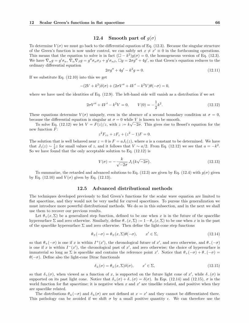
12 Scalar Green’s functions in flat spacetime 66
12.4 Smooth part of g(σ)
To determine V (σ) we must go back to the differential equation of Eq. (12.3). Because the singular structureof the Green’s function is now under control, we can safely set x 6= x′ ≡ 0 in the forthcoming operations.This means that the equation to solve is in fact ( − k2)g(σ) = 0, the homogeneous version of Eq. (12.3).We have ∇αg = g′σα, ∇α∇βg = g′′σασβ + g′σαβ , g = 2σg′′ + 4g′, so that Green’s equation reduces to theordinary differential equation
2σg′′ + 4g′ − k2g = 0. (12.11)
If we substitute Eq. (12.10) into this we get
−(2V + k2)δ(σ) + (2σV ′′ + 4V ′ − k2V )θ(−σ) = 0,
where we have used the identities of Eq. (12.9). The left-hand side will vanish as a distribution if we set
2σV ′′ + 4V ′ − k2V = 0, V (0) = −1
2k2. (12.12)
These equations determine V (σ) uniquely, even in the absence of a second boundary condition at σ = 0,because the differential equation is singular at σ = 0 while V is known to be smooth.
To solve Eq. (12.12) we let V = F (z)/z, with z := k√−2σ. This gives rise to Bessel’s equation for the
new function F :z2Fzz + zFz + (z2 − 1)F = 0.
The solution that is well behaved near z = 0 is F = aJ1(z), where a is a constant to be determined. We havethat J1(z) ∼ 1
2z for small values of z, and it follows that V ∼ a/2. From Eq. (12.12) we see that a = −k2.So we have found that the only acceptable solution to Eq. (12.12) is
V (σ) = − k√−2σ
J1
(k√−2σ
). (12.13)
To summarize, the retarded and advanced solutions to Eq. (12.3) are given by Eq. (12.4) with g(σ) givenby Eq. (12.10) and V (σ) given by Eq. (12.13).
12.5 Advanced distributional methods
The techniques developed previously to find Green’s functions for the scalar wave equation are limited toflat spacetime, and they would not be very useful for curved spacetimes. To pursue this generalization wemust introduce more powerful distributional methods. We do so in this subsection, and in the next we shalluse them to recover our previous results.
Let θ+(x,Σ) be a generalized step function, defined to be one when x is in the future of the spacelikehypersurface Σ and zero otherwise. Similarly, define θ−(x,Σ) := 1−θ+(x,Σ) to be one when x is in the pastof the spacelike hypersurface Σ and zero otherwise. Then define the light-cone step functions
θ±(−σ) = θ±(x,Σ)θ(−σ), x′ ∈ Σ, (12.14)
so that θ+(−σ) is one if x is within I+(x′), the chronological future of x′, and zero otherwise, and θ−(−σ)is one if x is within I−(x′), the chronological past of x′, and zero otherwise; the choice of hypersurface isimmaterial so long as Σ is spacelike and contains the reference point x′. Notice that θ+(−σ) + θ−(−σ) =θ(−σ). Define also the light-cone Dirac functionals
δ±(σ) = θ±(x,Σ)δ(σ), x′ ∈ Σ, (12.15)
so that δ+(σ), when viewed as a function of x, is supported on the future light cone of x′, while δ−(σ) issupported on its past light cone. Notice that δ+(σ) + δ−(σ) = δ(σ). In Eqs. (12.14) and (12.15), σ is theworld function for flat spacetime; it is negative when x and x′ are timelike related, and positive when theyare spacelike related.
The distributions θ±(−σ) and δ±(σ) are not defined at x = x′ and they cannot be differentiated there.This pathology can be avoided if we shift σ by a small positive quantity ε. We can therefore use the
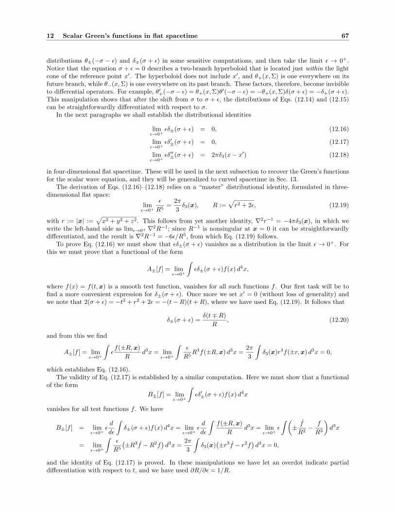
12 Scalar Green’s functions in flat spacetime 67
distributions θ±(−σ − ε) and δ±(σ + ε) in some sensitive computations, and then take the limit ε → 0+.Notice that the equation σ + ε = 0 describes a two-branch hyperboloid that is located just within the lightcone of the reference point x′. The hyperboloid does not include x′, and θ+(x,Σ) is one everywhere on itsfuture branch, while θ−(x,Σ) is one everywhere on its past branch. These factors, therefore, become invisibleto differential operators. For example, θ′+(−σ− ε) = θ+(x,Σ)θ′(−σ− ε) = −θ+(x,Σ)δ(σ+ ε) = −δ+(σ+ ε).This manipulation shows that after the shift from σ to σ + ε, the distributions of Eqs. (12.14) and (12.15)can be straightforwardly differentiated with respect to σ.
In the next paragraphs we shall establish the distributional identities
limε→0+
εδ±(σ + ε) = 0, (12.16)
limε→0+
εδ′±(σ + ε) = 0, (12.17)
limε→0+
εδ′′±(σ + ε) = 2πδ4(x− x′) (12.18)
in four-dimensional flat spacetime. These will be used in the next subsection to recover the Green’s functionsfor the scalar wave equation, and they will be generalized to curved spacetime in Sec. 13.
The derivation of Eqs. (12.16)–(12.18) relies on a “master” distributional identity, formulated in three-dimensional flat space:
limε→0+
ε
R5=
2π
3δ3(x), R :=
√r2 + 2ε, (12.19)
with r := |x| :=√x2 + y2 + z2. This follows from yet another identity, ∇2r−1 = −4πδ3(x), in which we
write the left-hand side as limε→0+ ∇2R−1; since R−1 is nonsingular at x = 0 it can be straightforwardlydifferentiated, and the result is ∇2R−1 = −6ε/R5, from which Eq. (12.19) follows.
To prove Eq. (12.16) we must show that εδ±(σ + ε) vanishes as a distribution in the limit ε → 0+. Forthis we must prove that a functional of the form
A±[f ] = limε→0+
∫εδ±(σ + ε)f(x) d4x,
where f(x) = f(t,x) is a smooth test function, vanishes for all such functions f . Our first task will be tofind a more convenient expression for δ±(σ + ε). Once more we set x′ = 0 (without loss of generality) andwe note that 2(σ + ε) = −t2 + r2 + 2ε = −(t−R)(t+R), where we have used Eq. (12.19). It follows that
δ±(σ + ε) =δ(t∓R)
R, (12.20)
and from this we find
A±[f ] = limε→0+
∫εf(±R,x)
Rd3x = lim
ε→0+
∫ε
R5R4f(±R,x) d3x =
2π
3
∫δ3(x)r4f(±r,x) d3x = 0,
which establishes Eq. (12.16).The validity of Eq. (12.17) is established by a similar computation. Here we must show that a functional
of the form
B±[f ] = limε→0+
∫εδ′±(σ + ε)f(x) d4x
vanishes for all test functions f . We have
B±[f ] = limε→0+
εd
dε
∫δ±(σ + ε)f(x) d4x = lim
ε→0+εd
dε
∫f(±R,x)
Rd3x = lim
ε→0+ε
∫ (± f
R2− f
R3
)d3x
= limε→0+
∫ε
R5
(±R3f −R2f
)d3x =
2π
3
∫δ3(x)
(±r3f − r2f
)d3x = 0,
and the identity of Eq. (12.17) is proved. In these manipulations we have let an overdot indicate partialdifferentiation with respect to t, and we have used ∂R/∂ε = 1/R.

12 Scalar Green’s functions in flat spacetime 68
To establish Eq. (12.18) we consider the functional
C±[f ] = limε→0+
∫εδ′′±(σ + ε)f(x) d4x
and show that it evaluates to 2πf(0,0). We have
C±[f ] = limε→0+
εd2
dε2
∫δ±(σ + ε)f(x) d4x = lim
ε→0+εd2
dε2
∫f(±R,x)
Rd3x
= limε→0+
ε
∫ (f
R3∓ 3
f
R4+ 3
f
R5
)d3x = 2π
∫δ3(x)
(1
3r2f ± rf + f
)d3x
= 2πf(0,0),
as required. This proves that Eq. (12.18) holds as a distributional identity in four-dimensional flat spacetime.
12.6 Alternative computation of the Green’s functions
The retarded and advanced Green’s functions for the scalar wave equation are now defined as the limit ofthe functions Gε±(x, x′) when ε→ 0+. For these we make the ansatz
Gε±(x, x′) = δ±(σ + ε) + V (σ)θ±(−σ − ε), (12.21)
and we shall prove that Gε±(x, x′) satisfies Eq. (12.3) in the limit. We recall that the distributions θ± andδ± were defined in the preceding subsection, and we assume that V (σ) is a smooth function of σ(x, x′) =12ηαβ(x − x′)α(x − x′)β ; because this function is smooth, it is not necessary to evaluate V at σ + ε inEq. (12.21). We recall also that θ+ and δ+ are nonzero when x is in the future of x′, while θ− and δ−are nonzero when x is in the past of x′. We will therefore prove that the retarded and advanced Green’sfunctions are of the form
Gret(x, x′) = lim
ε→0+Gε+(x, x′) = θ+(x,Σ)
[δ(σ) + V (σ)θ(−σ)
](12.22)
andGadv(x, x′) = lim
ε→0+Gε−(x, x′) = θ−(x,Σ)
[δ(σ) + V (σ)θ(−σ)
], (12.23)
where Σ is a spacelike hypersurface that contains x′. We will also determine the form of the function V (σ).The functions that appear in Eq. (12.21) can be straightforwardly differentiated. The manipulations are
similar to what was done in Sec. 12.4, and dropping all labels, we obtain ( − k2)G = 2σG′′ + 4G′ − k2G,with a prime indicating differentiation with respect to σ. From Eq. (12.21) we obtain G′ = δ′−V δ+V ′θ andG′′ = δ′′ − V δ′ − 2V ′δ + V ′′θ. The identities of Eq. (12.9) can be expressed as (σ + ε)δ′(σ + ε) = −δ(σ + ε)and (σ + ε)δ′′(σ + ε) = −2δ′(σ + ε), and combining this with our previous results gives
(− k2)Gε±(x, x′) = (−2V − k2)δ±(σ + ε) + (2σV ′′ + 4V ′ − k2V )θ±(−σ − ε)− 2εδ′′±(σ + ε) + 2V εδ′±(σ + ε) + 4V ′εδ±(σ + ε).
According to Eq. (12.16)–(12.18), the last two terms on the right-hand side disappear in the limit ε → 0+,and the third term becomes −4πδ4(x − x′). Provided that the first two terms vanish also, we recover( − k2)G(x, x′) = −4πδ4(x − x′) in the limit, as required. Thus, the limit of Gε±(x, x′) when ε → 0+ willindeed satisfy Green’s equation provided that V (σ) is a solution to
2σV ′′ + 4V ′ − k2V = 0, V (0) = −1
2k2; (12.24)
these are the same statements as in Eq. (12.12). The solution to these equations was produced in Eq. (12.13):
V (σ) = − k√−2σ
J1
(k√−2σ
), (12.25)
and this completely determines the Green’s functions of Eqs. (12.22) and (12.23).

13 Distributions in curved spacetime 69
13 Distributions in curved spacetime
The distributions introduced in Sec. 12.5 can also be defined in a four-dimensional spacetime with metricgαβ . Here we produce the relevant generalizations of the results derived in that section.
13.1 Invariant Dirac distribution
We first introduce δ4(x, x′), an invariant Dirac functional in a four-dimensional curved spacetime. This isdefined by the relations∫
V
f(x)δ4(x, x′)√−g d4x = f(x′),
∫V ′f(x′)δ4(x, x′)
√−g′ d4x′ = f(x), (13.1)
where f(x) is a smooth test function, V any four-dimensional region that contains x′, and V ′ any four-dimensional region that contains x. These relations imply that δ4(x, x′) is symmetric in its arguments, andit is easy to see that
δ4(x, x′) =δ4(x− x′)√−g =
δ4(x− x′)√−g′ = (gg′)−1/4δ4(x− x′), (13.2)
where δ4(x− x′) = δ(x0− x′0)δ(x1− x′1)δ(x2− x′2)δ(x3− x′3) is the ordinary (coordinate) four-dimensionalDirac functional. The relations of Eq. (13.2) are all equivalent because f(x)δ4(x, x′) = f(x′)δ4(x, x′) is adistributional identity; the last form is manifestly symmetric in x and x′.
The invariant Dirac distribution satisfies the identities
Ω···(x, x′)δ4(x, x′) =
[Ω···]δ4(x, x′),
(13.3)(gαα′(x, x
′)δ4(x, x′))
;α= −∂α′δ4(x, x′),
(gα′
α(x′, x)δ4(x, x′))
;α′= −∂αδ4(x, x′),
where Ω···(x, x′) is any bitensor and gαα′(x, x
′), gα′
α(x, x′) are parallel propagators. The first identity followsimmediately from the definition of the δ-function. The second and third identities are established by showingthat integration against a test function f(x) gives the same result from both sides. For example, the first ofthe Eqs. (13.1) implies ∫
V
f(x)∂α′δ4(x, x′)√−g d4x = ∂α′f(x′),
and on the other hand,
−∫V
f(x)(gαα′δ4(x, x′)
);α
√−g d4x = −∮∂V
f(x)gαα′δ4(x, x′)dΣα +[f,αg
αα′]
= ∂α′f(x′),
which establishes the second identity of Eq. (13.3). Notice that in these manipulations, the integrationsinvolve scalar functions of the coordinates x; the fact that these functions are also vectors with respect to x′
does not invalidate the procedure. The third identity of Eq. (13.3) is proved in a similar way.
13.2 Light-cone distributions
For the remainder of Sec. 13 we assume that x ∈ N (x′), so that a unique geodesic β links these two points.We then let σ(x, x′) be the curved spacetime world function, and we define light-cone step functions by
θ±(−σ) = θ±(x,Σ)θ(−σ), x′ ∈ Σ, (13.4)
where θ+(x,Σ) is one when x is in the future of the spacelike hypersurface Σ and zero otherwise, andθ−(x,Σ) = 1− θ+(x,Σ). These are immediate generalizations to curved spacetime of the objects defined inflat spacetime by Eq. (12.14). We have that θ+(−σ) is one when x is within I+(x′), the chronological futureof x′, and zero otherwise, and θ−(−σ) is one when x is within I−(x′), the chronological past of x′, and zerootherwise. We also have θ+(−σ) + θ−(−σ) = θ(−σ).

14 Scalar Green’s functions in curved spacetime 70
We define the curved-spacetime version of the light-cone Dirac functionals by
δ±(σ) = θ±(x,Σ)δ(σ), x′ ∈ Σ, (13.5)
an immediate generalization of Eq. (12.15). We have that δ+(σ), when viewed as a function of x, is supportedon the future light cone of x′, while δ−(σ) is supported on its past light cone. We also have δ+(σ) + δ−(σ) =δ(σ), and we recall that σ is negative when x and x′ are timelike related, and positive when they are spacelikerelated.
For the same reasons as those mentioned in Sec. 12.5, it is sometimes convenient to shift the argument ofthe step and δ-functions from σ to σ+ ε, where ε is a small positive quantity. With this shift, the light-conedistributions can be straightforwardly differentiated with respect to σ. For example, δ±(σ+ε) = −θ′±(−σ−ε),with a prime indicating differentiation with respect to σ.
We now prove that the identities of Eq. (12.16)–(12.18) generalize to
limε→0+
εδ±(σ + ε) = 0, (13.6)
limε→0+
εδ′±(σ + ε) = 0, (13.7)
limε→0+
εδ′′±(σ + ε) = 2πδ4(x, x′) (13.8)
in a four-dimensional curved spacetime; the only differences lie with the definition of the world function andthe fact that it is the invariant Dirac functional that appears in Eq. (13.8). To establish these identities incurved spacetime we use the fact that they hold in flat spacetime — as was shown in Sec. 12.5 — and thatthey are scalar relations that must be valid in any coordinate system if they are found to hold in one. Letus then examine Eqs. (13.6)–(13.7) in the Riemann normal coordinates of Sec. 8; these are denoted xα andare based at x′. We have that σ(x, x′) = 1
2ηαβ xαxβ and δ4(x, x′) = ∆(x, x′)δ4(x − x′) = δ4(x − x′), where
∆(x, x′) is the van Vleck determinant, whose coincidence limit is unity. In Riemann normal coordinates,therefore, Eqs. (13.6)–(13.8) take exactly the same form as Eqs. (12.16)–(12.18). Because the identities aretrue in flat spacetime, they must be true also in curved spacetime (in Riemann normal coordinates based atx′); and because these are scalar relations, they must be valid in any coordinate system.
14 Scalar Green’s functions in curved spacetime
14.1 Green’s equation for a massless scalar field in curved spacetime
We consider a massless scalar field Φ(x) in a curved spacetime with metric gαβ . The field satisfies the waveequation
(− ξR)Φ(x) = −4πµ(x), (14.1)
where = gαβ∇α∇β is the wave operator, R the Ricci scalar, ξ an arbitrary coupling constant, and µ(x) isa prescribed source. We seek a Green’s function G(x, x′) such that a solution to Eq. (14.1) can be expressedas
Φ(x) =
∫G(x, x′)µ(x′)
√−g′ d4x′, (14.2)
where the integration is over the entire spacetime. The wave equation for the Green’s function is
(− ξR)G(x, x′) = −4πδ4(x, x′), (14.3)
where δ4(x, x′) is the invariant Dirac functional introduced in Sec. 13.1. It is easy to verify that the fielddefined by Eq. (14.2) is truly a solution to Eq. (14.1).
We let G+(x, x′) be the retarded solution to Eq. (14.3), and G−(x, x′) is the advanced solution; whenviewed as functions of x, G+(x, x′) is nonzero in the causal future of x′, while G−(x, x′) is nonzero in itscausal past. We assume that the retarded and advanced Green’s functions exist as distributions and can bedefined globally in the entire spacetime.

14 Scalar Green’s functions in curved spacetime 71
14.2 Hadamard construction of the Green’s functions
Assuming throughout this subsection that x is restricted to the normal convex neighbourhood of x′, we makethe ansatz
G±(x, x′) = U(x, x′)δ±(σ) + V (x, x′)θ±(−σ), (14.4)
where U(x, x′) and V (x, x′) are smooth biscalars; the fact that the spacetime is no longer homogeneousmeans that these functions cannot depend on σ alone.
Before we substitute the Green’s functions of Eq. (14.4) into the differential equation of Eq. (14.3)we proceed as in Sec. 12.6 and shift σ by the small positive quantity ε. We shall therefore consider thedistributions
Gε±(x, x′) = U(x, x′)δ±(σ + ε) + V (x, x′)θ±(−θ − ε),and later recover the Green’s functions by taking the limit ε → 0+. Differentiation of these objects isstraightforward, and in the following manipulations we will repeatedly use the relation σασα = 2σ satisfiedby the world function. We will also use the distributional identities σδ±(σ+ ε) = −εδ±(σ+ ε), σδ′±(σ+ ε) =−δ±(σ + ε)− εδ′±(σ + ε), and σδ′′±(σ + ε) = −2δ′(σ + ε)− εδ′′(σ + ε). After a routine calculation we obtain
(− ξR)Gε± = −2εδ′′±(σ + ε)U + 2εδ′±(σ + ε)V + δ′±(σ + ε)
2U,ασα + (σαα − 4)U
+ δ±(σ + ε)
−2V,ασ
α + (2− σαα)V + (− ξR)U
+ θ±(−σ − ε)
(− ξR)V,
which becomes
(− ξR)G± = −4πδ4(x, x′)U + δ′±(σ)
2U,ασα + (σαα − 4)U
+ δ±(σ)
−2V,ασ
α + (2− σαα)V + (− ξR)U
+ θ±(−σ)
(− ξR)V
(14.5)
in the limit ε→ 0+, after using the identities of Eqs. (13.6)–(13.8).According to Eq. (14.3), the right-hand side of Eq. (14.5) should be equal to −4πδ4(x, x′). This imme-
diately gives us the coincidence condition [U]
= 1 (14.6)
for the biscalar U(x, x′). To eliminate the δ′± term we make its coefficient vanish:
2U,ασα + (σαα − 4)U = 0. (14.7)
As we shall now prove, these two equations determine U(x, x′) uniquely.Recall from Sec. 3.3 that σα is a vector at x that is tangent to the unique geodesic β that connects x to x′.
This geodesic is affinely parameterized by λ and a displacement along β is described by dxα = (σα/λ)dλ. Thefirst term of Eq. (14.7) therefore represents the logarithmic rate of change of U(x, x′) along β, and this can beexpressed as 2λdU/dλ. For the second term we recall from Sec. 7.1 the differential equation ∆−1(∆σα);α = 4satisfied by ∆(x, x′), the van Vleck determinant. This gives us σαα−4 = −∆−1∆,ασ
α = −∆−1λd∆/dλ, andEq. (14.7) becomes
λd
dλ
(2 lnU − ln ∆
)= 0.
It follows that U2/∆ is constant on β, and this must therefore be equal to its value at the starting pointx′: U2/∆ = [U2/∆] = 1, by virtue of Eq. (14.6) and the property [∆] = 1 of the van Vleck determinant.Because this statement must be true for all geodesics β that emanate from x′, we have found that the uniquesolution to Eqs. (14.6) and (14.7) is
U(x, x′) = ∆1/2(x, x′). (14.8)
We must still consider the remaining terms in Eq. (14.5). The δ± term can be eliminated by demandingthat its coefficient vanish when σ = 0. This, however, does not constrain its value away from the light cone,and we thus obtain information about V |σ=0 only. Denoting this by V (x, x′) — the restriction of V (x, x′)on the light cone σ(x, x′) = 0 — we have
V,ασα +
1
2
(σαα − 2
)V =
1
2
(− ξR
)U∣∣∣σ=0
, (14.9)

14 Scalar Green’s functions in curved spacetime 72
where we indicate that the right-hand side also must be restricted to the light cone. The first term ofEq. (14.9) can be expressed as λdV /dλ and this equation can be integrated along any null geodesic thatgenerates the null cone σ(x, x′) = 0. For these integrations to be well posed, however, we must provide initialvalues at x = x′. As we shall now see, these can be inferred from Eq. (14.9) and the fact that V (x, x′) mustbe smooth at coincidence.
Equations (7.4) and (14.8) imply that near coincidence, U(x, x′) admits the expansion
U = 1 +1
12Rα′β′σ
α′σβ′+O(λ3), (14.10)
where Rα′β′ is the Ricci tensor at x′ and λ is the affine-parameter distance to x (which can be either on oroff the light cone). Differentiation of this relation gives
U,α = −1
6gα′
αRα′β′σβ′ +O(λ2), U,α′ =
1
6Rα′β′σ
β′ +O(λ2), (14.11)
and eventually, [U]
=1
6R(x′). (14.12)
Using also [σαα] = 4, we find that the coincidence limit of Eq. (14.9) gives[V]
=1
12
(1− 6ξ
)R(x′), (14.13)
and this provides the initial values required for the integration of Eq. (14.9) on the null cone.Equations (14.9) and (14.13) give us a means to construct V (x, x′), the restriction of V (x, x′) on the null
cone σ(x, x′) = 0. These values can then be used as characteristic data for the wave equation
(− ξR)V (x, x′) = 0, (14.14)
which is obtained by elimination of the θ± term in Eq. (14.5). While this certainly does not constitutea practical method to compute the biscalar V (x, x′), these considerations show that V (x, x′) exists and isunique.
To summarize: We have shown that with U(x, x′) given by Eq. (14.8) and V (x, x′) determined uniquelyby the wave equation of Eq. (14.14) and the characteristic data constructed with Eqs. (14.9) and (14.13), theretarded and advanced Green’s functions of Eq. (14.4) do indeed satisfy Eq. (14.3). It should be emphasizedthat the construction provided in this subsection is restricted to N (x′), the normal convex neighbourhoodof the reference point x′.
14.3 Reciprocity
We shall now establish the following reciprocity relation between the (globally defined) retarded and advancedGreen’s functions:
G−(x′, x) = G+(x, x′). (14.15)
Before we get to the proof we observe that by virtue of Eq. (14.15), the biscalar V (x, x′) must be symmetricin its arguments:
V (x′, x) = V (x, x′). (14.16)
To go from Eq. (14.15) to Eq. (14.16) we simply note that when x ∈ N (x′) and belongs to I+(x′), thenG+(x, x′) = V (x, x′) and G−(x′, x) = V (x′, x).
To prove the reciprocity relation we invoke the identities
G+(x, x′)(− ξR)G−(x, x′′) = −4πG+(x, x′)δ4(x, x′′)
andG−(x, x′′)(− ξR)G+(x, x′) = −4πG−(x, x′′)δ4(x, x′)

14 Scalar Green’s functions in curved spacetime 73
and take their difference. On the left-hand side we have
G+(x, x′)G−(x, x′′)−G−(x, x′′)G+(x, x′) = ∇α(G+(x, x′)∇αG−(x, x′′)−G−(x, x′′)∇αG+(x, x′)
),
while the right-hand side gives
−4π(G+(x, x′)δ4(x, x′′)−G−(x, x′′)δ4(x, x′)
).
Integrating both sides over a large four-dimensional region V that contains both x′ and x′′, we obtain∮∂V
(G+(x, x′)∇αG−(x, x′′)−G−(x, x′′)∇αG+(x, x′)
)dΣα = −4π
(G+(x′′, x′)−G−(x′, x′′)
),
where ∂V is the boundary of V . Assuming that the Green’s functions fall off sufficiently rapidly at infinity(in the limit ∂V → ∞; this statement imposes some restriction on the spacetime’s asymptotic structure),we have that the left-hand side of the equation evaluates to zero in the limit. This gives us the statementG+(x′′, x′) = G−(x′, x′′), which is just Eq. (14.15) with x′′ replacing x.
14.4 Kirchhoff representation
Suppose that the values for a scalar field Φ(x′) and its normal derivative nα′∇α′Φ(x′) are known on a
spacelike hypersurface Σ. Suppose also that the scalar field satisfies the homogeneous wave equation
(− ξR)Φ(x) = 0. (14.17)
Then the value of the field at a point x in the future of Σ is given by Kirchhoff’s formula,
Φ(x) = − 1
4π
∫Σ
(G+(x, x′)∇α′Φ(x′)− Φ(x′)∇α′G+(x, x′)
)dΣα′ , (14.18)
where dΣα′ is the surface element on Σ. If nα′ is the future-directed unit normal, then dΣα′ = −nα′dV ,with dV denoting the invariant volume element on Σ; notice that dΣα′ is past directed.
To establish this result we start with the equations
G−(x′, x)(′ − ξR′)Φ(x′) = 0, Φ(x′)(′ − ξR′)G−(x′, x) = −4πδ4(x′, x)Φ(x′),
in which x and x′ refer to arbitrary points in spacetime. Taking their difference gives
∇α′(G−(x′, x)∇α′Φ(x′)− Φ(x′)∇α′G−(x′, x)
)= 4πδ4(x′, x)Φ(x′),
and this we integrate over a four-dimensional region V that is bounded in the past by the hypersurface Σ.We suppose that V contains x and we obtain∮
∂V
(G−(x′, x)∇α′Φ(x′)− Φ(x′)∇α′G−(x′, x)
)dΣα′ = 4πΦ(x),
where dΣα′ is the outward-directed surface element on the boundary ∂V . Assuming that the Green’s functionfalls off sufficiently rapidly into the future, we have that the only contribution to the hypersurface integral isthe one that comes from Σ. Since the surface element on Σ points in the direction opposite to the outward-directed surface element on ∂V , we must change the sign of the left-hand side to be consistent with theconvention adopted previously. With this change we have
Φ(x) = − 1
4π
∮∂V
(G−(x′, x)∇α′Φ(x′)− Φ(x′)∇α′G−(x′, x)
)dΣα′ ,
which is the same statement as Eq. (14.18) if we take into account the reciprocity relation of Eq. (14.15).

14 Scalar Green’s functions in curved spacetime 74
14.5 Singular and regular Green’s functions
In part IV of this review we will compute the retarded field of a moving scalar charge, and we will analyzeits singularity structure near the world line; this will be part of our effort to understand the effect of thefield on the particle’s motion. The retarded solution to the scalar wave equation is the physically relevantsolution because it properly incorporates outgoing-wave boundary conditions at infinity — the advancedsolution would come instead with incoming-wave boundary conditions. The retarded field is singular on theworld line because a point particle produces a Coulomb field that diverges at the particle’s position. In viewof this singular behaviour, it is a subtle matter to describe the field’s action on the particle, and to formulatemeaningful equations of motion.
When facing this problem in flat spacetime (recall the discussion of Sec. 1.3) it is convenient to decomposethe retarded Green’s function G+(x, x′) into a singular Green’s function GS(x, x′) := 1
2 [G+(x, x′)+G−(x, x′)]and a regular two-point function GR(x, x′) := 1
2 [G+(x, x′)−G−(x, x′)]. The singular Green’s function takesits name from the fact that it produces a field with the same singularity structure as the retarded solution:the diverging field near the particle is insensitive to the boundary conditions imposed at infinity. We notealso that GS(x, x′) satisfies the same wave equation as the retarded Green’s function (with a Dirac functionalas a source), and that by virtue of the reciprocity relations, it is symmetric in its arguments. The regulartwo-point function, on the other hand, takes its name from the fact that it satisfies the homogeneous waveequation, without the Dirac functional on the right-hand side; it produces a field that is regular on the worldline of the moving scalar charge. (We reserve the term “Green’s function” to a two-point function thatsatisfies the wave equation with a Dirac distribution on the right-hand side; when the source term is absent,the object is called a “two-point function”.)
Because the singular Green’s function is symmetric in its argument, it does not distinguish betweenpast and future, and it produces a field that contains equal amounts of outgoing and incoming radiation —the singular solution describes a standing wave at infinity. Removing GS(x, x′) from the retarded Green’sfunction will have the effect of removing the singular behaviour of the field without affecting the motion ofthe particle. The motion is not affected because it is intimately tied to the boundary conditions: If thewaves are outgoing, the particle loses energy to the radiation and its motion is affected; if the waves areincoming, the particle gains energy from the radiation and its motion is affected differently. With equalamounts of outgoing and incoming radiation, the particle neither loses nor gains energy and its interactionwith the scalar field cannot affect its motion. Thus, subtracting GS(x, x′) from the retarded Green’s functioneliminates the singular part of the field without affecting the motion of the scalar charge. The subtractionleaves behind the regular two-point function, which produces a field that is regular on the world line; it isthis field that will govern the motion of the particle. The action of this field is well defined, and it properlyencodes the outgoing-wave boundary conditions: the particle will lose energy to the radiation.
In this subsection we attempt a decomposition of the curved-spacetime retarded Green’s function intosingular and regular pieces. The flat-spacetime relations will have to be amended, however, because ofthe fact that in a curved spacetime, the advanced Green’s function is generally nonzero when x′ is in thechronological future of x. This implies that the value of the advanced field at x depends on events x′ thatwill unfold in the future; this dependence would be inherited by the regular field (which acts on the particleand determines its motion) if the naive definition GR(x, x′) := 1
2 [G+(x, x′)−G−(x, x′)] were to be adopted.We shall not adopt this definition. Instead, we shall follow Detweiler and Whiting [13] and introduce a
singular Green’s function with the properties
S1: GS(x, x′) satisfies the inhomogeneous scalar wave equation,
(− ξR)GS(x, x′) = −4πδ4(x, x′); (14.19)
S2: GS(x, x′) is symmetric in its arguments,
GS(x′, x) = GS(x, x′); (14.20)
S3: GS(x, x′) vanishes if x is in the chronological past or future of x′,
GS(x, x′) = 0 when x ∈ I±(x′). (14.21)

14 Scalar Green’s functions in curved spacetime 75
Properties S1 and S2 ensure that the singular Green’s function will properly reproduce the singular behaviourof the retarded solution without distinguishing between past and future; and as we shall see, property S3ensures that the support of the regular two-point function will not include the chronological future of x.
The regular two-point function is then defined by
GR(x, x′) = G+(x, x′)−GS(x, x′), (14.22)
where G+(x, x′) is the retarded Green’s function. This comes with the properties
R1: GR(x, x′) satisfies the homogeneous wave equation,
(− ξR)GR(x, x′) = 0; (14.23)
R2: GR(x, x′) agrees with the retarded Green’s function if x is in the chronological future of x′,
GR(x, x′) = G+(x, x′) when x ∈ I+(x′); (14.24)
R3: GR(x, x′) vanishes if x is in the chronological past of x′,
GR(x, x′) = 0 when x ∈ I−(x′). (14.25)
Property R1 follows directly from Eq. (14.22) and property S1 of the singular Green’s function. PropertiesR2 and R3 follow from S3 and the fact that the retarded Green’s function vanishes if x is in past of x′. Theproperties of the regular two-point function ensure that the corresponding regular field will be nonsingularat the world line, and will depend only on the past history of the scalar charge.
We must still show that such singular and regular Green’s functions can be constructed. This relies onthe existence of a two-point function H(x, x′) that would possess the properties
H1: H(x, x′) satisfies the homogeneous wave equation,
(− ξR)H(x, x′) = 0; (14.26)
H2: H(x, x′) is symmetric in its arguments,
H(x′, x) = H(x, x′); (14.27)
H3: H(x, x′) agrees with the retarded Green’s function if x is in the chronological future of x′,
H(x, x′) = G+(x, x′) when x ∈ I+(x′); (14.28)
H4: H(x, x′) agrees with the advanced Green’s function if x is in the chronological past of x′,
H(x, x′) = G−(x, x′) when x ∈ I−(x′). (14.29)
With a biscalar H(x, x′) satisfying these relations, a singular Green’s function defined by
GS(x, x′) =1
2
[G+(x, x′) +G−(x, x′)−H(x, x′)
](14.30)
will satisfy all the properties listed previously: S1 comes as a consequence of H1 and the fact that boththe advanced and the retarded Green’s functions are solutions to the inhomogeneous wave equation, S2follows directly from H2 and the definition of Eq. (14.30), and S3 comes as a consequence of H3, H4 and theproperties of the retarded and advanced Green’s functions.
The question is now: does such a function H(x, x′) exist? We will present a plausibility argument for anaffirmative answer. Later in this section we will see that H(x, x′) is guaranteed to exist in the local convexneighbourhood of x′, where it is equal to V (x, x′). And in Sec. 14.6 we will see that there exist particularspacetimes for which H(x, x′) can be defined globally.
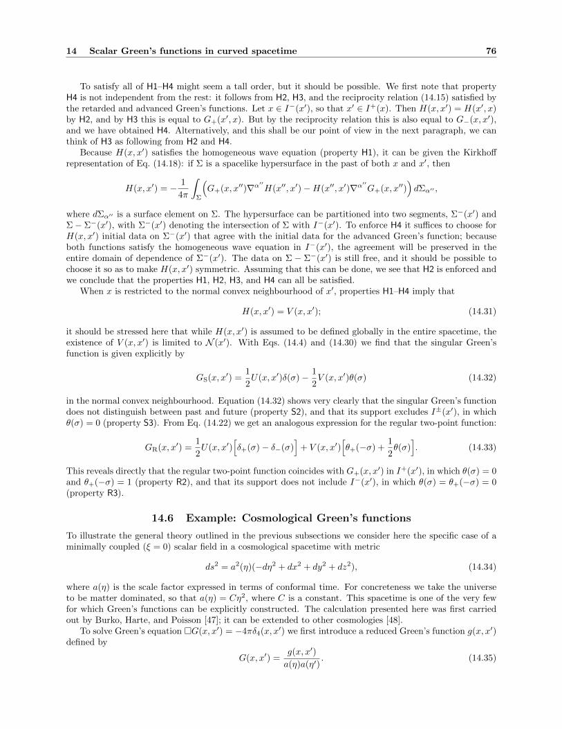
14 Scalar Green’s functions in curved spacetime 76
To satisfy all of H1–H4 might seem a tall order, but it should be possible. We first note that propertyH4 is not independent from the rest: it follows from H2, H3, and the reciprocity relation (14.15) satisfied bythe retarded and advanced Green’s functions. Let x ∈ I−(x′), so that x′ ∈ I+(x). Then H(x, x′) = H(x′, x)by H2, and by H3 this is equal to G+(x′, x). But by the reciprocity relation this is also equal to G−(x, x′),and we have obtained H4. Alternatively, and this shall be our point of view in the next paragraph, we canthink of H3 as following from H2 and H4.
Because H(x, x′) satisfies the homogeneous wave equation (property H1), it can be given the Kirkhoffrepresentation of Eq. (14.18): if Σ is a spacelike hypersurface in the past of both x and x′, then
H(x, x′) = − 1
4π
∫Σ
(G+(x, x′′)∇α′′H(x′′, x′)−H(x′′, x′)∇α′′G+(x, x′′)
)dΣα′′ ,
where dΣα′′ is a surface element on Σ. The hypersurface can be partitioned into two segments, Σ−(x′) andΣ− Σ−(x′), with Σ−(x′) denoting the intersection of Σ with I−(x′). To enforce H4 it suffices to choose forH(x, x′) initial data on Σ−(x′) that agree with the initial data for the advanced Green’s function; becauseboth functions satisfy the homogeneous wave equation in I−(x′), the agreement will be preserved in theentire domain of dependence of Σ−(x′). The data on Σ − Σ−(x′) is still free, and it should be possible tochoose it so as to make H(x, x′) symmetric. Assuming that this can be done, we see that H2 is enforced andwe conclude that the properties H1, H2, H3, and H4 can all be satisfied.
When x is restricted to the normal convex neighbourhood of x′, properties H1–H4 imply that
H(x, x′) = V (x, x′); (14.31)
it should be stressed here that while H(x, x′) is assumed to be defined globally in the entire spacetime, theexistence of V (x, x′) is limited to N (x′). With Eqs. (14.4) and (14.30) we find that the singular Green’sfunction is given explicitly by
GS(x, x′) =1
2U(x, x′)δ(σ)− 1
2V (x, x′)θ(σ) (14.32)
in the normal convex neighbourhood. Equation (14.32) shows very clearly that the singular Green’s functiondoes not distinguish between past and future (property S2), and that its support excludes I±(x′), in whichθ(σ) = 0 (property S3). From Eq. (14.22) we get an analogous expression for the regular two-point function:
GR(x, x′) =1
2U(x, x′)
[δ+(σ)− δ−(σ)
]+ V (x, x′)
[θ+(−σ) +
1
2θ(σ)
]. (14.33)
This reveals directly that the regular two-point function coincides with G+(x, x′) in I+(x′), in which θ(σ) = 0and θ+(−σ) = 1 (property R2), and that its support does not include I−(x′), in which θ(σ) = θ+(−σ) = 0(property R3).
14.6 Example: Cosmological Green’s functions
To illustrate the general theory outlined in the previous subsections we consider here the specific case of aminimally coupled (ξ = 0) scalar field in a cosmological spacetime with metric
ds2 = a2(η)(−dη2 + dx2 + dy2 + dz2), (14.34)
where a(η) is the scale factor expressed in terms of conformal time. For concreteness we take the universeto be matter dominated, so that a(η) = Cη2, where C is a constant. This spacetime is one of the very fewfor which Green’s functions can be explicitly constructed. The calculation presented here was first carriedout by Burko, Harte, and Poisson [47]; it can be extended to other cosmologies [48].
To solve Green’s equation G(x, x′) = −4πδ4(x, x′) we first introduce a reduced Green’s function g(x, x′)defined by
G(x, x′) =g(x, x′)
a(η)a(η′). (14.35)

14 Scalar Green’s functions in curved spacetime 77
Substitution yields (− ∂2
∂η2+∇2 +
2
η2
)g(x, x′) = −4πδ(η − η′)δ3(x− x′), (14.36)
where x = (x, y, z) is a vector in three-dimensional flat space, and ∇2 is the Laplacian operator in this space.We next expand g(x, x′) in terms of plane-wave solutions to Laplace’s equation,
g(x, x′) =1
(2π)3
∫g(η, η′;k) eik·(x−x
′) d3k, (14.37)
and we substitute this back into Eq. (14.36). The result, after also Fourier transforming δ3(x − x′), is anordinary differential equation for g(η, η′;k):(
d2
dη2+ k2 − 2
η2
)g = 4πδ(η − η′), (14.38)
where k2 = k · k. To generate the retarded Green’s function we set
g+(η, η′;k) = θ(η − η′) g(η, η′; k), (14.39)
in which we indicate that g depends only on the modulus of the vector k. To generate the advanced Green’sfunction we would set instead g−(η, η′;k) = θ(η′ − η) g(η, η′; k). The following manipulations will referspecifically to the retarded Green’s function; they are easily adapted to the case of the advanced Green’sfunction.
Substitution of Eq. (14.39) into Eq. (14.38) reveals that g must satisfy the homogeneous equation(d2
dη2+ k2 − 2
η2
)g = 0, (14.40)
together with the boundary conditions
g(η = η′; k) = 0,dg
dη(η = η′; k) = 4π. (14.41)
Inserting Eq. (14.39) into Eq. (14.37) and integrating over the angular variables associated with the vectork yields
g+(x, x′) =θ(∆η)
2π2R
∫ ∞0
g(η, η′; k) k sin(kR) dk, (14.42)
where ∆η := η − η′ and R := |x− x′|.Equation (14.40) has cos(k∆η)−(kη)−1 sin(k∆η) and sin(k∆η)+(kη)−1 cos(k∆η) as linearly independent
solutions, and g(η, η′; k) must be given by a linear superposition. The coefficients can be functions of η′, andafter imposing Eqs. (14.41) we find that the appropriate combination is
g(η, η′; k) =4π
k
[(1 +
1
k2ηη′
)sin(k∆η)− ∆η
kηη′cos(k∆η)
]. (14.43)
Substituting this into Eq. (14.42) and using the identity (2/π)∫∞
0sin(ωx) sin(ωx′) dω = δ(x−x′)− δ(x+x′)
yields
g+(x, x′) =δ(∆η −R)
R+θ(∆η)
ηη′2
π
∫ ∞0
1
ksin(k∆η) cos(kR) dk
after integration by parts. The integral evaluates to θ(∆η −R).We have arrived at
g+(x, x′) =δ(η − η′ − |x− x′|)
|x− x′| +θ(η − η′ − |x− x′|)
ηη′(14.44)

15 Electromagnetic Green’s functions 78
for our final expression for the retarded Green’s function. The advanced Green’s function is given insteadby
g−(x, x′) =δ(η − η′ + |x− x′|)
|x− x′| +θ(−η + η′ − |x− x′|)
ηη′. (14.45)
The distributions g±(x, x′) are solutions to the reduced Green’s equation of Eq. (14.36). The actual Green’sfunctions are obtained by substituting Eqs. (14.44) and (14.45) into Eq. (14.35). We note that the supportof the retarded Green’s function is given by η − η′ ≥ |x − x′|, while the support of the advanced Green’sfunction is given by η − η′ ≤ −|x− x′|.
It may be verified that the symmetric two-point function
h(x, x′) =1
ηη′(14.46)
satisfies all of the properties H1–H4 listed in Sec. 14.5; it may thus be used to define singular and regularGreen’s functions. According to Eq. (14.30) the singular Green’s function is given by
gS(x, x′) =1
2|x− x′|[δ(η − η′ − |x− x′|) + δ(η − η′ + |x− x′|)
]+
1
2ηη′
[θ(η − η′ − |x− x′|)− θ(η − η′ + |x− x′|)
](14.47)
and its support is limited to the interval −|x−x′| ≤ η− η′ ≤ |x−x′|. According to Eq. (14.22) the regulartwo-point function is given by
gR(x, x′) =1
2|x− x′|[δ(η − η′ − |x− x′|)− δ(η − η′ + |x− x′|)
]+
1
2ηη′
[θ(η − η′ − |x− x′|) + θ(η − η′ + |x− x′|)
]; (14.48)
its support is given by η − η′ ≥ −|x − x′| and for η − η′ ≥ |x − x′| the regular two-point function agreeswith the retarded Green’s function.
As a final observation we note that for this cosmological spacetime, the normal convex neighbourhood ofany point x consists of the whole spacetime manifold (which excludes the cosmological singularity at a = 0).The Hadamard construction of the Green’s functions is therefore valid globally, a fact that is immediatelyrevealed by Eqs. (14.44) and (14.45).
15 Electromagnetic Green’s functions
15.1 Equations of electromagnetism
The electromagnetic field tensor Fαβ = ∇αAβ − ∇βAα is expressed in terms of a vector potential Aα. Inthe Lorenz gauge ∇αAα = 0, the vector potential satisfies the wave equation
Aα −RαβAβ = −4πjα, (15.1)
where = gαβ∇α∇β is the wave operator, Rαβ the Ricci tensor, and jα a prescribed current density. Thewave equation enforces the condition ∇αjα = 0, which expresses charge conservation.
The solution to the wave equation is written as
Aα(x) =
∫Gαβ′(x, x
′)jβ′(x′)
√−g′ d4x′, (15.2)
in terms of a Green’s function Gαβ′(x, x′) that satisfies
Gαβ′(x, x′)−Rαβ(x)Gββ′(x, x
′) = −4πgαβ′(x, x′)δ4(x, x′), (15.3)
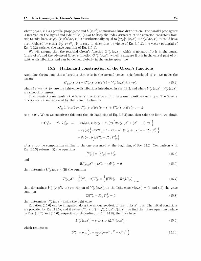
15 Electromagnetic Green’s functions 79
where gαβ′(x, x′) is a parallel propagator and δ4(x, x′) an invariant Dirac distribution. The parallel propagator
is inserted on the right-hand side of Eq. (15.3) to keep the index structure of the equation consistent fromside to side; because gαβ′(x, x
′)δ4(x, x′) is distributionally equal to [gαβ′ ]δ4(x, x′) = δα′
β′δ4(x, x′), it could have
been replaced by either δα′
β′ or δαβ . It is easy to check that by virtue of Eq. (15.3), the vector potential ofEq. (15.2) satisfies the wave equation of Eq. (15.1).
We will assume that the retarded Green’s function G α+β′(x, x
′), which is nonzero if x is in the causalfuture of x′, and the advanced Green’s function G α
−β′(x, x′), which is nonzero if x is in the causal past of x′,
exist as distributions and can be defined globally in the entire spacetime.
15.2 Hadamard construction of the Green’s functions
Assuming throughout this subsection that x is in the normal convex neighbourhood of x′, we make theansatz
G α±β′(x, x
′) = Uαβ′(x, x′)δ±(σ) + V αβ′(x, x
′)θ±(−σ), (15.4)
where θ±(−σ), δ±(σ) are the light-cone distributions introduced in Sec. 13.2, and where Uαβ′(x, x′), V αβ′(x, x
′)are smooth bitensors.
To conveniently manipulate the Green’s functions we shift σ by a small positive quantity ε. The Green’sfunctions are then recovered by the taking the limit of
Gε α± β′(x, x′) := Uαβ′(x, x
′)δ±(σ + ε) + V αβ′(x, x′)θ±(−σ − ε)
as ε→ 0+. When we substitute this into the left-hand side of Eq. (15.3) and then take the limit, we obtain
G α±β′ −RαβG β
±β′ = −4πδ4(x, x′)Uαβ′ + δ′±(σ)
2Uαβ′;γσγ + (σγγ − 4)Uαβ′
+ δ±(σ)
−2V αβ′;γσ
γ + (2− σγγ)V αβ′ +Uαβ′ −RαβUββ′
+ θ±(−σ)V αβ′ −RαβV ββ′
after a routine computation similar to the one presented at the beginning of Sec. 14.2. Comparison withEq. (15.3) returns: (i) the equations [
Uαβ′]
=[gαβ′
]= δα
′
β′ (15.5)
and2Uαβ′;γσ
γ + (σγγ − 4)Uαβ′ = 0 (15.6)
that determine Uαβ′(x, x′); (ii) the equation
V αβ′;γσγ +
1
2(σγγ − 2)V αβ′ =
1
2
(Uαβ′ −RαβUββ′
)∣∣∣σ=0
(15.7)
that determines V αβ′(x, x′), the restriction of V αβ′(x, x
′) on the light cone σ(x, x′) = 0; and (iii) the waveequation
V αβ′ −RαβV ββ′ = 0 (15.8)
that determines V αβ′(x, x′) inside the light cone.
Equation (15.6) can be integrated along the unique geodesic β that links x′ to x. The initial conditionsare provided by Eq. (15.5), and if we set Uαβ′(x, x
′) = gαβ′(x, x′)U(x, x′), we find that these equations reduce
to Eqs. (14.7) and (14.6), respectively. According to Eq. (14.8), then, we have
Uαβ′(x, x′) = gαβ′(x, x
′)∆1/2(x, x′), (15.9)
which reduces to
Uαβ′ = gαβ′(
1 +1
12Rγ′δ′σ
γ′σδ′+O(λ3)
)(15.10)
15 Electromagnetic Green’s functions 80
near coincidence, with λ denoting the affine-parameter distance between x′ and x. Differentiation of thisrelation gives
Uαβ′;γ =1
2gγ′
γ
(gαα′R
α′
β′γ′δ′ −1
3gαβ′Rγ′δ′
)σδ′+O(λ2), (15.11)
Uαβ′;γ′ =1
2
(gαα′R
α′
β′γ′δ′ +1
3gαβ′Rγ′δ′
)σδ′+O(λ2), (15.12)
and eventually, [Uαβ′
]=
1
6δα′
β′R(x′). (15.13)
Similarly, Eq. (15.7) can be integrated along each null geodesic that generates the null cone σ(x, x′) = 0.The initial values are obtained by taking the coincidence limit of this equation, using Eqs. (15.5), (15.13),and the additional relation [σγγ ] = 4. We arrive at
[V αβ′
]= −1
2
(Rα′
β′ −1
6δα′
β′R′). (15.14)
With the characteristic data obtained by integrating Eq. (15.7), the wave equation of Eq. (15.8) admits aunique solution.
To summarize, the retarded and advanced electromagnetic Green’s functions are given by Eq. (15.4)with Uαβ′(x, x
′) given by Eq. (15.9) and V αβ′(x, x′) determined by Eq. (15.8) and the characteristic data
constructed with Eqs. (15.7) and (15.14). It should be emphasized that the construction provided in thissubsection is restricted to N (x′), the normal convex neighbourhood of the reference point x′.
15.3 Reciprocity and Kirchhoff representation
Like their scalar counterparts, the (globally defined) electromagnetic Green’s functions satisfy a reciprocityrelation, the statement of which is
G−β′α(x′, x) = G+αβ′(x, x
′). (15.15)
The derivation of Eq. (15.15) is virtually identical to what was presented in Sec. 14.3, and we shall notpresent the details. It suffices to mention that it is based on the identities
G+αβ′(x, x
′)(G α−γ′′(x, x
′′)−RαγG γ−γ′′(x, x
′′))
= −4πG+αβ′(x, x
′)gαγ′′(x, x′′)δ4(x, x′′)
andG−αγ′′(x, x
′′)(G α
+β′(x, x′)−RαγG γ
+β′(x, x′))
= −4πG−αγ′′(x, x′′)gαβ′(x, x
′)δ4(x, x′).
A direct consequence of the reciprocity relation is
Vβ′α(x′, x) = Vαβ′(x, x′), (15.16)
the statement that the bitensor Vαβ′(x, x′) is symmetric in its indices and arguments.
The Kirchhoff representation for the electromagnetic vector potential is formulated as follows. Supposethat Aα(x) satisfies the homogeneous version of Eq. (15.1) and that initial values Aα
′(x′), nβ
′∇β′Aα′(x′) are
specified on a spacelike hypersurface Σ. Then the value of the potential at a point x in the future of Σ isgiven by
Aα(x) = − 1
4π
∫Σ
(G α
+β′(x, x′)∇γ′Aβ′(x′)−Aβ′(x′)∇γ′G α
+β′(x, x′)
)dΣγ′ , (15.17)
where dΣγ′ = −nγ′dV is a surface element on Σ; nγ′ is the future-directed unit normal and dV is theinvariant volume element on the hypersurface. The derivation of Eq. (15.17) is virtually identical to whatwas presented in Sec. 14.4.

15 Electromagnetic Green’s functions 81
15.4 Relation with scalar Green’s functions
In a spacetime that satisfies the Einstein field equations in vacuum, so that Rαβ = 0 everywhere in thespacetime, the (retarded and advanced) electromagnetic Green’s functions satisfy the identities [4]
G α±β′;α = −G±;β′ , (15.18)
where G± are the corresponding scalar Green’s functions.To prove this we differentiate Eq. (15.3) covariantly with respect to xα and use Eq. (13.3) to express
the right-hand side as +4π∂β′δ4(x, x′). After repeated use of Ricci’s identity to permute the ordering of thecovariant derivatives on the left-hand side, we arrive at the equation
(−Gαβ′;α
)= −4π∂β′δ4(x, x′); (15.19)
all terms involving the Riemann tensor disappear by virtue of the fact that the spacetime is Ricci-flat.Because Eq. (15.19) is also the differential equation satisfied by G;β′ , and because the solutions are chosento satisfy the same boundary conditions, we have established the validity of Eq. (15.18).
15.5 Singular and regular Green’s functions
We shall now construct singular and regular Green’s functions for the electromagnetic field. The treatmenthere parallels closely what was presented in Sec. 14.5, and the reader is referred to that section for a morecomplete discussion.
We begin by introducing the bitensor Hαβ′(x, x
′) with properties
H1: Hαβ′(x, x
′) satisfies the homogeneous wave equation,
Hαβ′(x, x
′)−Rαβ(x)Hββ′(x, x
′) = 0; (15.20)
H2: Hαβ′(x, x
′) is symmetric in its indices and arguments,
Hβ′α(x′, x) = Hαβ′(x, x′); (15.21)
H3: Hαβ′(x, x
′) agrees with the retarded Green’s function if x is in the chronological future of x′,
Hαβ′(x, x
′) = G α+β′(x, x
′) when x ∈ I+(x′); (15.22)
H4: Hαβ′(x, x
′) agrees with the advanced Green’s function if x is in the chronological past of x′,
Hαβ′(x, x
′) = G α−β′(x, x
′) when x ∈ I−(x′). (15.23)
It is easy to prove that property H4 follows from H2, H3, and the reciprocity relation (15.15) satisfied by theretarded and advanced Green’s functions. That such a bitensor exists can be argued along the same lines asthose presented in Sec. 14.5.
Equipped with the bitensor Hαβ′(x, x
′) we define the singular Green’s function to be
G αS β′(x, x
′) =1
2
[G α
+β′(x, x′) +G α
−β′(x, x′)−Hα
β′(x, x′)]. (15.24)
This comes with the properties
S1: G αS β′(x, x
′) satisfies the inhomogeneous wave equation,
G αS β′(x, x
′)−Rαβ(x)G βS β′(x, x
′) = −4πgαβ′(x, x′)δ4(x, x′); (15.25)
S2: G αS β′(x, x
′) is symmetric in its indices and arguments,
GSβ′α(x′, x) = GS
αβ′(x, x′); (15.26)
16 Gravitational Green’s functions 82
S3: G αS β′(x, x
′) vanishes if x is in the chronological past or future of x′,
G αS β′(x, x
′) = 0 when x ∈ I±(x′). (15.27)
These can be established as consequences of H1–H4 and the properties of the retarded and advanced Green’sfunctions.
The regular two-point function is then defined by
G αR β′(x, x
′) = G α+β′(x, x
′)−G αS β′(x, x
′), (15.28)
and it comes with the properties
R1: G αR β′(x, x
′) satisfies the homogeneous wave equation,
G αR β′(x, x
′)−Rαβ(x)G βR β′(x, x
′) = 0; (15.29)
R2: G αR β′(x, x
′) agrees with the retarded Green’s function if x is in the chronological future of x′,
G αR β′(x, x
′) = G α+β′(x, x
′) when x ∈ I+(x′); (15.30)
R3: G αR β′(x, x
′) vanishes if x is in the chronological past of x′,
G αR β′(x, x
′) = 0 when x ∈ I−(x′). (15.31)
Those follow immediately from S1–S3 and the properties of the retarded Green’s function.When x is restricted to the normal convex neighbourhood of x′, we have the explicit relations
Hαβ′(x, x
′) = V αβ′(x, x′), (15.32)
G αS β′(x, x
′) =1
2Uαβ′(x, x
′)δ(σ)− 1
2V αβ′(x, x
′)θ(σ), (15.33)
G αR β′(x, x
′) =1
2Uαβ′(x, x
′)[δ+(σ)− δ−(σ)
]+ V αβ′(x, x
′)[θ+(−σ) +
1
2θ(σ)
]. (15.34)
From these we see clearly that the singular Green’s function does not distinguish between past and future(property S2), and that its support excludes I±(x′) (property S3). We see also that the regular two-pointfunction coincides with G α
+β′(x, x′) in I+(x′) (property R2), and that its support does not include I−(x′)
(property R3).
16 Gravitational Green’s functions
16.1 Equations of linearized gravity
We are given a background spacetime for which the metric gαβ satisfies the Einstein field equations invacuum. We then perturb the metric from gαβ to
gαβ = gαβ + hαβ . (16.1)
The metric perturbation hαβ is assumed to be small, and when working out the Einstein field equations tobe satisfied by the new metric gαβ , we work consistently to first order in hαβ . To simplify the expressionswe use the trace-reversed potentials γαβ defined by
γαβ = hαβ −1
2
(gγδhγδ
)gαβ , (16.2)
and we impose the Lorenz gauge condition,γαβ;β = 0. (16.3)
16 Gravitational Green’s functions 83
In this equation, and in all others below, indices are raised and lowered with the background metric gαβ .Similarly, the connection involved in Eq. (16.3), and in all other equations below, is the one that is compatiblewith the background metric. If Tαβ is the perturbing energy-momentum tensor, then by virtue of thelinearized Einstein field equations the perturbation field obeys the wave equation
γαβ + 2R α βγ δ γ
γδ = −16πTαβ , (16.4)
in which = gαβ∇α∇β is the wave operator and Rγαδβ the Riemann tensor. In first-order perturbation
theory, the energy-momentum tensor must be conserved in the background spacetime: Tαβ;β = 0.The solution to the wave equation is written as
γαβ(x) = 4
∫Gαβγ′δ′(x, x
′)T γ′δ′(x′)
√−g′ d4x′, (16.5)
in terms of a Green’s function Gαβγ′δ′(x, x′) that satisfies [140]
Gαβγ′δ′(x, x′) + 2R α β
γ δ (x)Gγδγ′δ′(x, x′) = −4πg
(αγ′(x, x
′)gβ)δ′(x, x
′)δ4(x, x′), (16.6)
where gαγ′(x, x′) is a parallel propagator and δ4(x, x′) an invariant Dirac functional. The parallel propagators
are inserted on the right-hand side of Eq. (16.6) to keep the index structure of the equation consistent fromside to side; in particular, both sides of the equation are symmetric in α and β, and in γ′ and δ′. It is easy tocheck that by virtue of Eq. (16.6), the perturbation field of Eq. (16.5) satisfies the wave equation of Eq. (16.4).Once γαβ is known, the metric perturbation can be reconstructed from the relation hαβ = γαβ− 1
2 (gγδγγδ)gαβ .
We will assume that the retarded Green’s function G αβ+ γ′δ′(x, x
′), which is nonzero if x is in the causal
future of x′, and the advanced Green’s function G αβ− γ′δ′(x, x
′), which is nonzero if x is in the causal past ofx′, exist as distributions and can be defined globally in the entire background spacetime.
16.2 Hadamard construction of the Green’s functions
Assuming throughout this subsection that x is in the normal convex neighbourhood of x′, we make theansatz
G αβ± γ′δ′(x, x
′) = Uαβγ′δ′(x, x′)δ±(σ) + V αβγ′δ′(x, x
′)θ±(−σ), (16.7)
where θ±(−σ), δ±(σ) are the light-cone distributions introduced in Sec. 13.2, and where Uαβγ′δ′(x, x′),
V αβγ′δ′(x, x′) are smooth bitensors.
To conveniently manipulate the Green’s functions we shift σ by a small positive quantity ε. The Green’sfunctions are then recovered by the taking the limit of
Gε αβ± γ′δ′(x, x′) = Uαβγ′δ′(x, x
′)δ±(σ + ε) + V αβγ′δ′(x, x′)θ±(−σ − ε)
as ε→ 0+. When we substitute this into the left-hand side of Eq. (16.6) and then take the limit, we obtain
G αβ± γ′δ′ + 2R α β
γ δ Gγδ± γ′δ′ = −4πδ4(x, x′)Uαβγ′δ′ + δ′±(σ)
2Uαβγ′δ′;γσ
γ + (σγγ − 4)Uαβγ′δ′
+ δ±(σ)−2V αβγ′δ′;γσ
γ + (2− σγγ)V αβγ′δ′ +Uαβγ′δ′ + 2R α βγ δ U
γδγ′δ′
+ θ±(−σ)
V αβγ′δ′ + 2R α β
γ δ Vγδγ′δ′
after a routine computation similar to the one presented at the beginning of Sec. 14.2. Comparison withEq. (16.6) returns: (i) the equations [
Uαβγ′δ′]
=[g
(αγ′g
β)δ′
]= δ
(α′
γ′δβ′)δ′ (16.8)
and2Uαβγ′δ′;γσ
γ + (σγγ − 4)Uαβγ′δ′ = 0 (16.9)
16 Gravitational Green’s functions 84
that determine Uαβγ′δ′(x, x′); (ii) the equation
V αβγ′δ′;γσγ +
1
2(σγγ − 2)V αβγ′δ′ =
1
2
(Uαβγ′δ′ + 2R α β
γ δ Uγδγ′δ′
)∣∣∣σ=0
(16.10)
that determine V αβγ′δ′(x, x′), the restriction of V αβγ′δ′(x, x
′) on the light cone σ(x, x′) = 0; and (iii) the waveequation
V αβγ′δ′ + 2R α βγ δ V
γδγ′δ′ = 0 (16.11)
that determines V αβγ′δ′(x, x′) inside the light cone.
Equation (16.9) can be integrated along the unique geodesic β that links x′ to x. The initial conditions
are provided by Eq. (16.8), and if we set Uαβγ′δ′(x, x′) = g
(αγ′g
β)δ′U(x, x′), we find that these equations reduce
to Eqs. (14.7) and (14.6), respectively. According to Eq. (14.8), then, we have
Uαβγ′δ′(x, x′) = g
(αγ′(x, x
′)gβ)δ′(x, x
′)∆1/2(x, x′), (16.12)
which reduces toUαβγ′δ′ = g
(αγ′g
β)δ′
(1 +O(λ3)
)(16.13)
near coincidence, with λ denoting the affine-parameter distance between x′ and x; there is no term of orderλ2 because by assumption, the background Ricci tensor vanishes at x′ (as it does in the entire spacetime).Differentiation of this relation gives
Uαβγ′δ′;ε =1
2g
(αα′g
β)β′g
ε′
ε
(Rα′
γ′ε′ι′δβ′
δ′ +Rα′
δ′ε′ι′δβ′
γ′
)σι′+O(λ2), (16.14)
Uαβγ′δ′;ε′ =1
2g
(αα′g
β)β′
(Rα′
γ′ε′ι′δβ′
δ′ +Rα′
δ′ε′ι′δβ′
γ′
)σι′+O(λ2), (16.15)
and eventually, [Uαβγ′δ′ ] = 0; (16.16)
this last result follows from the fact that [Uαβγ′δ′;ει] is antisymmetric in the last pair of indices.Similarly, Eq. (16.10) can be integrated along each null geodesic that generates the null cone σ(x, x′) = 0.
The initial values are obtained by taking the coincidence limit of this equation, using Eqs. (16.8), (16.16),and the additional relation [σγγ ] = 4. We arrive at[
V αβγ′δ′]
=1
2
(Rα′ β′
γ′ δ′ +Rβ′ α′
γ′ δ′
). (16.17)
With the characteristic data obtained by integrating Eq. (16.10), the wave equation of Eq. (16.11) admits aunique solution.
To summarize, the retarded and advanced gravitational Green’s functions are given by Eq. (16.7) with
Uαβγ′δ′(x, x′) given by Eq. (16.12) and V αβγ′δ′(x, x
′) determined by Eq. (16.11) and the characteristic dataconstructed with Eqs. (16.10) and (16.17). It should be emphasized that the construction provided in thissubsection is restricted to N (x′), the normal convex neighbourhood of the reference point x′.
16.3 Reciprocity and Kirchhoff representation
The (globally defined) gravitational Green’s functions satisfy the reciprocity relation
G−γ′δ′αβ(x′, x) = G+αβγ′δ′(x, x
′). (16.18)
The derivation of this result is virtually identical to what was presented in Secs. 14.3 and 15.3. A directconsequence of the reciprocity relation is the statement
Vγ′δ′αβ(x′, x) = Vαβγ′δ′(x, x′). (16.19)
The Kirchhoff representation for the trace-reversed gravitational perturbation γαβ is formulated as fol-
lows. Suppose that γαβ(x) satisfies the homogeneous version of Eq. (16.4) and that initial values γα′β′(x′),

16 Gravitational Green’s functions 85
nγ′∇γ′γα
′β′(x′) are specified on a spacelike hypersurface Σ. Then the value of the perturbation field at apoint x in the future of Σ is given by
γαβ(x) = − 1
4π
∫Σ
(G αβ
+ γ′δ′(x, x′)∇ε′γγ′δ′(x′)− γγ′δ′(x′)∇ε′G αβ
+ γ′δ′(x, x′)
)dΣε′ , (16.20)
where dΣε′ = −nε′dV is a surface element on Σ; nε′ is the future-directed unit normal and dV is theinvariant volume element on the hypersurface. The derivation of Eq. (16.20) is virtually identical to whatwas presented in Secs. 14.4 and 15.3.
16.4 Relation with electromagnetic and scalar Green’s functions
In a spacetime that satisfies the Einstein field equations in vacuum, so that Rαβ = 0 everywhere in thespacetime, the (retarded and advanced) gravitational Green’s functions satisfy the identities [17]
G αβ± γ′δ′;β = −G α
±(γ′;δ′) (16.21)
andgγ′δ′G αβ
± γ′δ′ = gαβG±, (16.22)
where G α±β′ are the corresponding electromagnetic Green’s functions, and G± the corresponding scalar
Green’s functions.To prove Eq. (16.21) we differentiate Eq. (16.6) covariantly with respect to xβ , use Eq. (13.3) to work
on the right-hand side, and invoke Ricci’s identity to permute the ordering of the covariant derivatives onthe left-hand side. After simplification and involvement of the Ricci-flat condition (which, together with the
Bianchi identities, implies that R ;βαγβδ = 0), we arrive at the equation
(−Gαβγ′δ′;β
)= −4πgα(γ′∂δ′)δ4(x, x′). (16.23)
Because this is also the differential equation satisfied by Gα(β′;γ′), and because the solutions are chosen to
satisfy the same boundary conditions, we have established the validity of Eq. (16.21).
The identity of Eq. (16.22) follows simply from the fact that gγ′δ′Gαβγ′δ′ and gαβG satisfy the same
tensorial wave equation in a Ricci-flat spacetime.
16.5 Singular and regular Green’s functions
We shall now construct singular and regular Green’s functions for the linearized gravitational field. Thetreatment here parallels closely what was presented in Secs. 14.5 and 15.5.
We begin by introducing the bitensor Hαβγ′δ′(x, x
′) with properties
H1: Hαβγ′δ′(x, x
′) satisfies the homogeneous wave equation,
Hαβγ′δ′(x, x
′) + 2R α βγ δ (x)Hγδ
γ′δ′(x, x′) = 0; (16.24)
H2: Hαβγ′δ′(x, x
′) is symmetric in its indices and arguments,
Hγ′δ′αβ(x′, x) = Hαβγ′δ′(x, x′); (16.25)
H3: Hαβγ′δ′(x, x
′) agrees with the retarded Green’s function if x is in the chronological future of x′,
Hαβγ′δ′(x, x
′) = G αβ+ γ′δ′(x, x
′) when x ∈ I+(x′); (16.26)
H4: Hαβγ′δ′(x, x
′) agrees with the advanced Green’s function if x is in the chronological past of x′,
Hαβγ′δ′(x, x
′) = G αβ− γ′δ′(x, x
′) when x ∈ I−(x′). (16.27)

16 Gravitational Green’s functions 86
It is easy to prove that property H4 follows from H2, H3, and the reciprocity relation (16.18) satisfied by theretarded and advanced Green’s functions. That such a bitensor exists can be argued along the same lines asthose presented in Sec. 14.5.
Equipped with Hαβγ′δ′(x, x
′) we define the singular Green’s function to be
G αβS γ′δ′(x, x
′) =1
2
[G αβ
+ γ′δ′(x, x′) +G αβ
− γ′δ′(x, x′)−Hαβ
γ′δ′(x, x′)]. (16.28)
This comes with the properties
S1: G αβS γ′δ′(x, x
′) satisfies the inhomogeneous wave equation,
G αβS γ′δ′(x, x
′) + 2R α βγ δ (x)G γδ
S γ′δ′(x, x′) = −4πg
(αγ′(x, x
′)gβ)δ′(x, x
′)δ4(x, x′); (16.29)
S2: G αβS γ′δ′(x, x
′) is symmetric in its indices and arguments,
GSγ′δ′αβ(x′, x) = GS
αβγ′δ′(x, x′); (16.30)
S3: G αβS γ′δ′(x, x
′) vanishes if x is in the chronological past or future of x′,
G αβS γ′δ′(x, x
′) = 0 when x ∈ I±(x′). (16.31)
These can be established as consequences of H1–H4 and the properties of the retarded and advanced Green’sfunctions.
The regular two-point function is then defined by
G αβR γ′δ′(x, x
′) = G αβ+ γ′δ′(x, x
′)−G αβS γ′δ′(x, x
′), (16.32)
and it comes with the properties
R1: G αβR γ′δ′(x, x
′) satisfies the homogeneous wave equation,
G αβR γ′δ′(x, x
′) + 2R α βγ δ (x)G γδ
R γ′δ′(x, x′) = 0; (16.33)
R2: G αβR γ′δ′(x, x
′) agrees with the retarded Green’s function if x is in the chronological future of x′,
G αβR γ′δ′(x, x
′) = G αβ+ γ′δ′(x, x
′) when x ∈ I+(x′); (16.34)
R3: G αβR γ′δ′(x, x
′) vanishes if x is in the chronological past of x′,
G αβR γ′δ′(x, x
′) = 0 when x ∈ I−(x′). (16.35)
Those follow immediately from S1–S3 and the properties of the retarded Green’s function.When x is restricted to the normal convex neighbourhood of x′, we have the explicit relations
Hαβγ′δ′(x, x
′) = V αβγ′δ′(x, x′), (16.36)
G αβS γ′δ′(x, x
′) =1
2Uαβγ′δ′(x, x
′)δ(σ)− 1
2V αβγ′δ′(x, x
′)θ(σ), (16.37)
G αβR γ′δ′(x, x
′) =1
2Uαβγ′δ′(x, x
′)[δ+(σ)− δ−(σ)
]+ V αβγ′δ′(x, x
′)[θ+(−σ) +
1
2θ(σ)
]. (16.38)
From these we see clearly that the singular Green’s function does not distinguish between past and future(property S2), and that its support excludes I±(x′) (property S3). We see also that the regular two-point
function coincides with G αβ+ γ′δ′(x, x
′) in I+(x′) (property R2), and that its support does not include I−(x′)(property R3).

17 Motion of a scalar charge 87
Part IV
Motion of point particles
17 Motion of a scalar charge
17.1 Dynamics of a point scalar charge
A point particle carries a scalar charge q and moves on a world line γ described by relations zµ(λ), in whichλ is an arbitrary parameter. The particle generates a scalar potential Φ(x) and a field Φα(x) := ∇αΦ(x).The dynamics of the entire system is governed by the action
S = Sfield + Sparticle + Sinteraction, (17.1)
where Sfield is an action functional for a free scalar field in a spacetime with metric gαβ , Sparticle is the actionof a free particle moving on a world line γ in this spacetime, and Sinteraction is an interaction term thatcouples the field to the particle.
The field action is given by
Sfield = − 1
8π
∫ (gαβΦαΦβ + ξRΦ2
)√−g d4x, (17.2)
where the integration is over all of spacetime; the field is coupled to the Ricci scalar R by an arbitraryconstant ξ. The particle action is
Sparticle = −m0
∫γ
dτ, (17.3)
where m0 is the bare mass of the particle and dτ =√−gµν(z)zµzν dλ is the differential of proper time
along the world line; we use an overdot on zµ(λ) to indicate differentiation with respect to the parameter λ.Finally, the interaction term is given by
Sinteraction = q
∫γ
Φ(z) dτ = q
∫Φ(x)δ4(x, z)
√−g d4xdτ. (17.4)
Notice that both Sparticle and Sinteraction are invariant under a reparameterization λ → λ′(λ) of the worldline.
Demanding that the total action be stationary under a variation δΦ(x) of the field configuration yieldsthe wave equation (
− ξR)Φ(x) = −4πµ(x) (17.5)
for the scalar potential, with a charge density µ(x) defined by
µ(x) = q
∫γ
δ4(x, z) dτ. (17.6)
These equations determine the field Φα(x) once the motion of the scalar charge is specified. On the otherhand, demanding that the total action be stationary under a variation δzµ(λ) of the world line yields theequations of motion
m(τ)Duµ
dτ= q(gµν + uµuν
)Φν(z) (17.7)
for the scalar charge. We have here adopted τ as the parameter on the world line, and introduced the four-velocity uµ(τ) := dzµ/dτ . The dynamical mass that appears in Eq. (17.7) is defined by m(τ) := m0− qΦ(z),which can also be expressed in differential form as
dm
dτ= −qΦµ(z)uµ. (17.8)

17 Motion of a scalar charge 88
x
<
>
v
u
Figure 9: The region within the dashed boundary represents the normal convex neighbourhood of the pointx. The world line γ enters the neighbourhood at proper time τ< and exits at proper time τ>. Also shownare the retarded point z(u) and the advanced point z(v).
It should be clear that Eqs. (17.7) and (17.8) are valid only in a formal sense, because the scalar potentialobtained from Eqs. (17.5) and (17.6) diverges on the world line. Before we can make sense of these equationswe have to analyze the field’s singularity structure near the world line.
17.2 Retarded potential near the world line
The retarded solution to Eq. (17.5) is Φ(x) =∫G+(x, x′)µ(x′)
√g′ d4x′, where G+(x, x′) is the retarded
Green’s function introduced in Sec. 14. After substitution of Eq. (17.6) we obtain
Φ(x) = q
∫γ
G+(x, z) dτ, (17.9)
in which z(τ) gives the description of the world line γ. Because the retarded Green’s function is definedglobally in the entire spacetime, Eq. (17.9) applies to any field point x.
We now specialize Eq. (17.9) to a point x near the world line; see Fig. 9. We let N (x) be the normalconvex neighbourhood of this point, and we assume that the world line traverses N (x). Let τ< be the valueof the proper-time parameter at which γ enters N (x) from the past, and let τ> be its value when the worldline leaves N (x). Then Eq. (17.9) can be broken up into the three integrals
Φ(x) = q
∫ τ<
−∞G+(x, z) dτ + q
∫ τ>
τ<
G+(x, z) dτ + q
∫ ∞τ>
G+(x, z) dτ.
The third integration vanishes because x is then in the past of z(τ), and G+(x, z) = 0. For the secondintegration, x is the normal convex neighbourhood of z(τ), and the retarded Green’s function can be expressedin the Hadamard form produced in Sec. 14.2. This gives∫ τ>
τ<
G+(x, z) dτ =
∫ τ>
τ<
U(x, z)δ+(σ) dτ +
∫ τ>
τ<
V (x, z)θ+(−σ) dτ,
and to evaluate this we refer back to Sec. 10 and let x′ := z(u) be the retarded point associated with x;these points are related by σ(x, x′) = 0 and r := σα′u
α′ is the retarded distance between x and the worldline. We resume the index convention of Sec. 10: to tensors at x we assign indices α, β, etc.; to tensors at

17 Motion of a scalar charge 89
x′ we assign indices α′, β′, etc.; and to tensors at a generic point z(τ) on the world line we assign indices µ,ν, etc.
To perform the first integration we change variables from τ to σ, noticing that σ increases as z(τ) passesthrough x′. The change of σ on the world line is given by dσ := σ(x, z + dz) − σ(x, z) = σµu
µ dτ , and wefind that the first integral evaluates to U(x, z)/(σµu
µ) with z identified with x′. The second integration iscut off at τ = u by the step function, and we obtain our final expression for the retarded potential of a pointscalar charge:
Φ(x) =q
rU(x, x′) + q
∫ u
τ<
V (x, z) dτ + q
∫ τ<
−∞G+(x, z) dτ. (17.10)
This expression applies to a point x sufficiently close to the world line that there exists a nonempty inter-section between N (x) and γ.
17.3 Field of a scalar charge in retarded coordinates
When we differentiate the potential of Eq. (17.10) we must keep in mind that a variation in x induces avariation in x′ because the new points x + δx and x′ + δx′ must also be linked by a null geodesic — youmay refer back to Sec. 10.2 for a detailed discussion. This means, for example, that the total variation ofU(x, x′) is δU = U(x + δx, x′ + δx′)− U(x, x′) = U;αδx
α + U;α′uα′ δu. The gradient of the scalar potential
is therefore given by
Φα(x) = − q
r2U(x, x′)∂αr +
q
rU;α(x, x′) +
q
rU;α′(x, x
′)uα′∂αu+ qV (x, x′)∂αu+ Φtail
α (x), (17.11)
where the “tail integral” is defined by
Φtailα (x) = q
∫ u
τ<
∇αV (x, z) dτ + q
∫ τ<
−∞∇αG+(x, z) dτ
= q
∫ u−
−∞∇αG+(x, z) dτ. (17.12)
In the second form of the definition we integrate ∇αG+(x, z) from τ = −∞ to almost τ = u, but we cutthe integration short at τ = u− := u− 0+ to avoid the singular behaviour of the retarded Green’s functionat σ = 0. This limiting procedure gives rise to the first form of the definition, with the advantage that theintegral need not be broken up into contributions that refer to N (x) and its complement, respectively.
We shall now expand Φα(x) in powers of r, and express the results in terms of the retarded coordinates(u, r,Ωa) introduced in Sec. 10. It will be convenient to decompose Φα(x) in the tetrad (eα0 , e
αa ) that is
obtained by parallel transport of (uα′, eα
′
a ) on the null geodesic that links x to x′ := z(u); this constructionis detailed in Sec. 10. The expansion relies on Eq. (10.29) for ∂αu, Eq. (10.31) for ∂αr, and we shall need
U(x, x′) = 1 +1
12r2(R00 + 2R0aΩa +RabΩ
aΩb)
+O(r3), (17.13)
which follows from Eq. (14.10) and the relation σα′
= −r(uα′ + Ωaeα′
a ) first encountered in Eq. (10.7); recallthat
R00(u) = Rα′β′uα′uβ
′, R0a(u) = Rα′β′u
α′eβ′
a , Rab(u) = Rα′β′eα′
a eβ′
b
are frame components of the Ricci tensor evaluated at x′. We shall also need the expansions
U;α(x, x′) =1
6rgα
′
α
(Rα′0 +Rα′bΩ
b)
+O(r2) (17.14)
and
U;α′(x, x′)uα
′= −1
6r(R00 +R0aΩa
)+O(r2) (17.15)
which follow from Eqs. (14.11); recall from Eq. (10.4) that the parallel propagator can be expressed asgα′
α = uα′e0α + eα
′
a eaα. And finally, we shall need
V (x, x′) =1
12
(1− 6ξ
)R+O(r), (17.16)

17 Motion of a scalar charge 90
a relation that was first established in Eq. (14.13); here R := R(u) is the Ricci scalar evaluated at x′.Collecting all these results gives
Φ0(u, r,Ωa) := Φα(x)eα0 (x)
=q
raaΩa +
1
2qRa0b0ΩaΩb +
1
12
(1− 6ξ
)qR+ Φtail
0 +O(r), (17.17)
Φa(u, r,Ωa) := Φα(x)eαa (x)
= − q
r2Ωa −
q
rabΩ
bΩa −1
3qRb0c0ΩbΩcΩa −
1
6q(Ra0b0Ωb −Rab0cΩbΩc
)+
1
12q[R00 −RbcΩbΩc − (1− 6ξ)R
]Ωa +
1
6q(Ra0 +RabΩ
b)
+ Φtaila +O(r), (17.18)
where aa = aα′eα′
a are the frame components of the acceleration vector,
Ra0b0(u) = Rα′γ′β′δ′eα′
a uγ′eβ
′
b uδ′ , Rab0c(u) = Rα′γ′β′δ′e
α′
a eγ′
b uβ′eδ
′
c
are frame components of the Riemann tensor evaluated at x′, and
Φtail0 (u) = Φtail
α′ (x′)uα′, Φtail
a (u) = Φtailα′ (x′)eα
′
a (17.19)
are the frame components of the tail integral evaluated at x′. Equations (17.17) and (17.18) show clearlythat Φα(x) is singular on the world line: the field diverges as r−2 when r → 0, and many of the terms thatstay bounded in the limit depend on Ωa and therefore possess a directional ambiguity at r = 0.
17.4 Field of a scalar charge in Fermi normal coordinates
The gradient of the scalar potential can also be expressed in the Fermi normal coordinates of Sec. 9. Toeffect this translation we make x := z(t) the new reference point on the world line. We resume here thenotation of Sec. 11 and assign indices α, β, . . . to tensors at x. The Fermi normal coordinates are denoted(t, s, ωa), and we let (eα0 , e
αa ) be the tetrad at x that is obtained by parallel transport of (uα, eαa ) on the
spacelike geodesic that links x to x.Our first task is to decompose Φα(x) in the tetrad (eα0 , e
αa ), thereby defining Φ0 := Φαe
α0 and Φa := Φαe
αa .
For this purpose we use Eqs. (11.7), (11.8), (17.17), and (17.18) to obtain
Φ0 =[1 +O(r2)
]Φ0 +
[r(1− abΩb
)aa +
1
2r2aa +
1
2r2Ra0b0Ωb +O(r3)
]Φa
= −1
2qaaΩa +
1
12(1− 6ξ)qR+ Φtail
0 +O(r)
and
Φa =[δba +
1
2r2abaa −
1
2r2Rba0cΩ
c +O(r3)]Φb +
[raa +O(r2)
]Φ0
= − q
r2Ωa −
q
rabΩ
bΩa +1
2qabΩ
baa −1
3qRb0c0ΩbΩcΩa −
1
6qRa0b0Ωb − 1
3qRab0cΩ
bΩc
+1
12q[R00 −RbcΩbΩc − (1− 6ξ)R
]Ωa +
1
6q(Ra0 +RabΩ
b)
+ Φtaila +O(r),
where all frame components are still evaluated at x′, except for Φtail0 and Φtail
a which are evaluated at x.We must still translate these results into the Fermi normal coordinates (t, s, ωa). For this we involve
Eqs. (11.4), (11.5), and (11.6), from which we deduce, for example,
1
r2Ωa =
1
s2ωa +
1
2saa −
3
2sabω
bωa −3
4abω
baa +15
8
(abω
b)2ωa +
3
8a0ωa −
1
3aa
+ abωbωa +
1
6Ra0b0ω
b − 1
2Rb0c0ω
bωcωa −1
3Rab0cω
bωc +O(s)
and1
rabΩ
bΩa =1
sabω
bωa +1
2abω
baa −3
2
(abω
b)2ωa −
1
2a0ωa − abωbωa +O(s),

17 Motion of a scalar charge 91
in which all frame components (on the right-hand side of these relations) are now evaluated at x; to obtain thesecond relation we expressed aa(u) as aa(t)− saa(t) +O(s2) since according to Eq. (11.4), u = t− s+O(s2).
Collecting these results yields
Φ0(t, s, ωa) := Φα(x)eα0 (x)
= −1
2qaaω
a +1
12(1− 6ξ)qR+ Φtail
0 +O(s), (17.20)
Φa(t, s, ωa) := Φα(x)eαa (x)
= − q
s2ωa −
q
2s
(aa − abωbωa
)+
3
4qabω
baa −3
8q(abω
b)2ωa +
1
8qa0ωa +
1
3qaa
− 1
3qRa0b0ω
b +1
6qRb0c0ω
bωcωa +1
12q[R00 −Rbcωbωc − (1− 6ξ)R
]ωa
+1
6q(Ra0 +Rabω
b)
+ Φtaila +O(s). (17.21)
In these expressions, aa(t) = aαeαa are the frame components of the acceleration vector evaluated at x,
a0(t) = aαuα and aa(t) = aαe
αa are frame components of its covariant derivative, Ra0b0(t) = Rαγβδe
αau
γeβb uδ
are frame components of the Riemann tensor evaluated at x,
R00(t) = Rαβuαuβ , R0a(t) = Rαβu
αeβa , Rab(t) = Rαβeαaeβb
are frame components of the Ricci tensor, and R(t) is the Ricci scalar evaluated at x. Finally, we have that
Φtail0 (t) = Φtail
α (x)uα, Φtaila (t) = Φtail
α (x)eαa (17.22)
are the frame components of the tail integral — see Eq. (17.12) — evaluated at x := z(t).We shall now compute the averages of Φ0 and Φa over S(t, s), a two-surface of constant t and s; these
will represent the mean value of the field at a fixed proper distance away from the world line, as measured ina reference frame that is momentarily comoving with the particle. The two-surface is charted by angles θA
(A = 1, 2) and it is described, in the Fermi normal coordinates, by the parametric relations xa = sωa(θA);a canonical choice of parameterization is ωa = (sin θ cosφ, sin θ sinφ, cos θ). Introducing the transformationmatrices ωaA := ∂ωa/∂θA, we find from Eq. (9.16) that the induced metric on S(t, s) is given by
ds2 = s2[ωAB −
1
3s2RAB +O(s3)
]dθAdθB , (17.23)
where ωAB := δabωaAω
bB is the metric of the unit two-sphere, and where RAB := Racbdω
aAω
cωbBωd depends
on t and the angles θA. From this we infer that the element of surface area is given by
dA = s2[1− 1
6s2Rcacb(t)ω
aωb +O(s3)]dω, (17.24)
where dω =√
det[ωAB ] d2θ is an element of solid angle — in the canonical parameterization, dω = sin θ dθdφ.Integration of Eq. (17.24) produces the total surface area of S(t, s), and A = 4πs2[1− 1
18s2Rabab +O(s3)].
The averaged fields are defined by⟨Φ0
⟩(t, s) =
1
A
∮S(t,s)
Φ0(t, s, θA) dA,⟨Φa⟩(t, s) =
1
A
∮S(t,s)
Φa(t, s, θA) dA, (17.25)
where the quantities to be integrated are scalar functions of the Fermi normal coordinates. The results
1
4π
∮ωa dω = 0,
1
4π
∮ωaωb dω =
1
3δab,
1
4π
∮ωaωbωc dω = 0, (17.26)
are easy to establish, and we obtain⟨Φ0
⟩=
1
12(1− 6ξ)qR+ Φtail
0 +O(s), (17.27)⟨Φa⟩
= − q
3saa +
1
3qaa +
1
6qRa0 + Φtail
a +O(s). (17.28)

17 Motion of a scalar charge 92
The averaged field is still singular on the world line. Regardless, we shall take the formal limit s→ 0 of theexpressions displayed in Eqs. (17.27) and (17.28). In the limit the tetrad (eα0 , e
αa ) reduces to (uα, eαa ), and we
can reconstruct the field at x by invoking the completeness relations δαβ
= −uαuβ + eαaeaβ. We thus obtain
⟨Φα⟩
= lims→0
(− q
3s
)aα −
1
12(1− 6ξ)qRuα + q
(gαβ + uαuβ
)(1
3aβ +
1
6Rβγu
γ
)+ Φtail
α , (17.29)
where the tail integral can be copied from Eq. (17.12),
Φtailα (x) = q
∫ t−
−∞∇αG+(x, z) dτ. (17.30)
The tensors appearing in Eq. (17.29) all refer to x := z(t), which now stands for an arbitrary point on theworld line γ.
17.5 Singular and regular fields
The singular potential
ΦS(x) = q
∫γ
GS(x, z) dτ (17.31)
is the (unphysical) solution to Eqs. (17.5) and (17.6) that is obtained by adopting the singular Green’sfunction of Eq. (14.30) instead of the retarded Green’s function. As we shall see, the resulting singular fieldΦSα(x) reproduces the singular behaviour of the retarded solution; the difference, ΦR
α(x) = Φα(x)−ΦSα(x), is
regular on the world line.To evaluate the integral of Eq. (17.31) we assume once more that x is sufficiently close to γ that the
world line traverses N (x); refer back to Fig. 9. As before we let τ< and τ> be the values of the proper-timeparameter at which γ enters and leaves N (x), respectively. Then Eq. (17.31) can be broken up into the threeintegrals
ΦS(x) = q
∫ τ<
−∞GS(x, z) dτ + q
∫ τ>
τ<
GS(x, z) dτ + q
∫ ∞τ>
GS(x, z) dτ.
The first integration vanishes because x is then in the chronological future of z(τ), and GS(x, z) = 0 byEq. (14.21). Similarly, the third integration vanishes because x is then in the chronological past of z(τ). Forthe second integration, x is the normal convex neighbourhood of z(τ), the singular Green’s function can beexpressed in the Hadamard form of Eq. (14.32), and we have∫ τ>
τ<
GS(x, z) dτ =1
2
∫ τ>
τ<
U(x, z)δ+(σ) dτ +1
2
∫ τ>
τ<
U(x, z)δ−(σ) dτ − 1
2
∫ τ>
τ<
V (x, z)θ(σ) dτ.
To evaluate these we re-introduce the retarded point x′ := z(u) and let x′′ := z(v) be the advanced pointassociated with x; we recall from Sec. 11.4 that these points are related by σ(x, x′′) = 0 and that radv :=−σα′′uα
′′is the advanced distance between x and the world line.
To perform the first integration we change variables from τ to σ, noticing that σ increases as z(τ) passesthrough x′; the integral evaluates to U(x, x′)/r. We do the same for the second integration, but we notice nowthat σ decreases as z(τ) passes through x′′; the integral evaluates to U(x, x′′)/radv. The third integration isrestricted to the interval u ≤ τ ≤ v by the step function, and we obtain our final expression for the singularpotential of a point scalar charge:
ΦS(x) =q
2rU(x, x′) +
q
2radvU(x, x′′)− 1
2q
∫ v
u
V (x, z) dτ. (17.32)
We observe that ΦS(x) depends on the state of motion of the scalar charge between the retarded time uand the advanced time v; contrary to what was found in Sec. 17.2 for the retarded potential, there is nodependence on the particle’s remote past.

17 Motion of a scalar charge 93
We use the techniques of Sec. 17.3 to differentiate the potential of Eq. (17.32). We find
ΦSα(x) = − q
2r2U(x, x′)∂αr −
q
2radv2U(x, x′′)∂αradv +
q
2rU;α(x, x′) +
q
2rU;α′(x, x
′)uα′∂αu
+q
2radvU;α(x, x′′) +
q
2radvU;α′′(x, x
′′)uα′′∂αv +
1
2qV (x, x′)∂αu−
1
2qV (x, x′′)∂αv
− 1
2q
∫ v
u
∇αV (x, z) dτ, (17.33)
and we would like to express this as an expansion in powers of r. For this we shall rely on results alreadyestablished in Sec. 17.3, as well as additional expansions that will involve the advanced point x′′. Those wedevelop now.
We recall first that a relation between retarded and advanced times was worked out in Eq. (11.12), thatan expression for the advanced distance was displayed in Eq. (11.13), and that Eqs. (11.14) and (11.15) giveexpansions for ∂αv and ∂αradv, respectively.
To derive an expansion for U(x, x′′) we follow the general method of Sec. 11.4 and define a functionU(τ) := U(x, z(τ)) of the proper-time parameter on γ. We have that
U(x, x′′) := U(v) = U(u+ ∆′) = U(u) + U(u)∆′ +1
2U(u)∆′2 +O
(∆′3),
where overdots indicate differentiation with respect to τ , and where ∆′ := v − u. The leading term U(u) :=U(x, x′) was worked out in Eq. (17.13), and the derivatives of U(τ) are given by
U(u) = U;α′uα′ = −1
6r(R00 +R0aΩa
)+O(r2)
and
U(u) = U;α′β′uα′uβ
′+ U;α′a
α′ =1
6R00 +O(r),
according to Eqs. (17.15) and (14.11). Combining these results together with Eq. (11.12) for ∆′ gives
U(x, x′′) = 1 +1
12r2(R00 − 2R0aΩa +RabΩ
aΩb)
+O(r3), (17.34)
which should be compared with Eq. (17.13). It should be emphasized that in Eq. (17.34) and all equationsbelow, the frame components of the Ricci tensor are evaluated at the retarded point x′ := z(u), and notat the advanced point. The preceding computation gives us also an expansion for U;α′′u
α′′ := U(v) =
U(u) + U(u)∆′ +O(∆′2). This becomes
U;α′′(x, x′′)uα
′′=
1
6r(R00 −R0aΩa
)+O(r2), (17.35)
which should be compared with Eq. (17.15).We proceed similarly to derive an expansion for U;α(x, x′′). Here we introduce the functions Uα(τ) :=
U;α(x, z(τ)) and express U;α(x, x′′) as Uα(v) = Uα(u) + Uα(u)∆′ + O(∆′2). The leading term Uα(u) :=U;α(x, x′) was computed in Eq. (17.14), and
Uα(u) = U;αβ′uβ′ = −1
6gα′
αRα′0 +O(r)
follows from Eq. (14.11). Combining these results together with Eq. (11.12) for ∆′ gives
U;α(x, x′′) = −1
6rgα
′
α
(Rα′0 −Rα′bΩb
)+O(r2), (17.36)
and this should be compared with Eq. (17.14).The last expansion we shall need is
V (x, x′′) =1
12
(1− 6ξ
)R+O(r), (17.37)

17 Motion of a scalar charge 94
which follows at once from Eq. (17.16) and the fact that V (x, x′′) − V (x, x′) = O(r); the Ricci scalar isevaluated at the retarded point x′.
It is now a straightforward (but tedious) matter to substitute these expansions (all of them!) intoEq. (17.33) and obtain the projections of the singular field ΦS
α(x) in the same tetrad (eα0 , eαa ) that was
employed in Sec. 17.3. This gives
ΦS0(u, r,Ωa) := ΦS
α(x)eα0 (x)
=q
raaΩa +
1
2qRa0b0ΩaΩb +O(r), (17.38)
ΦSa(u, r,Ωa) := ΦS
α(x)eαa (x)
= − q
r2Ωa −
q
rabΩ
bΩa −1
3qaa −
1
3qRb0c0ΩbΩcΩa −
1
6q(Ra0b0Ωb −Rab0cΩbΩc
)+
1
12q[R00 −RbcΩbΩc − (1− 6ξ)R
]Ωa +
1
6qRabΩ
b, (17.39)
in which all frame components are evaluated at the retarded point x′ := z(u). Comparison of these expres-sions with Eqs. (17.17) and (17.18) reveals that the retarded and singular fields share the same singularitystructure.
The difference between the retarded field of Eqs. (17.17), (17.18) and the singular field of Eqs. (17.38),(17.39) defines the regular field ΦR
α(x). Its frame components are
ΦR0 =
1
12(1− 6ξ)qR+ Φtail
0 +O(r), (17.40)
ΦRa =
1
3qaa +
1
6qRa0 + Φtail
a +O(r), (17.41)
and we see that ΦRα(x) is a regular vector field on the world line. There is therefore no obstacle in evaluating
the regular field directly at x = x′, where the tetrad (eα0 , eαa ) becomes (uα
′, eα
′
a ). Reconstructing the field atx′ from its frame components, we obtain
ΦRα′(x
′) = − 1
12(1− 6ξ)qRuα′ + q
(gα′β′ + uα′uβ′
)(1
3aβ′+
1
6Rβ′
γ′uγ′)
+ Φtailα′ , (17.42)
where the tail term can be copied from Eq. (17.12),
Φtailα′ (x′) = q
∫ u−
−∞∇α′G+(x′, z) dτ. (17.43)
The tensors appearing in Eq. (17.42) all refer to the retarded point x′ := z(u), which now stands for anarbitrary point on the world line γ.
17.6 Equations of motion
The retarded field Φα(x) of a point scalar charge is singular on the world line, and this behaviour makesit difficult to understand how the field is supposed to act on the particle and affect its motion. The field’ssingularity structure was analyzed in Secs. 17.3 and 17.4, and in Sec. 17.5 it was shown to originate from thesingular field ΦS
α(x); the regular field ΦRα(x) = Φα(x) − ΦS
α(x) was then shown to be regular on the worldline.
To make sense of the retarded field’s action on the particle we temporarily model the scalar charge notas a point particle, but as a small hollow shell that appears spherical when observed in a reference framethat is momentarily comoving with the particle; the shell’s radius is s0 in Fermi normal coordinates, and itis independent of the angles contained in the unit vector ωa. The net force acting at proper time τ on thishollow shell is the average of qΦα(τ, s0, ω
a) over the surface of the shell. Assuming that the field on the shellis equal to the field of a point particle evaluated at s = s0, and ignoring terms that disappear in the limits0 → 0, we obtain from Eq. (17.29)
q⟨Φµ⟩
= −(δm)aµ −1
12(1− 6ξ)q2Ruµ + q2
(gµν + uµuν
)(1
3aν +
1
6Rνλu
λ
)+ qΦtail
µ , (17.44)
17 Motion of a scalar charge 95
where
δm := lims0→0
q2
3s0(17.45)
is formally a divergent quantity and
qΦtailµ = q2
∫ τ−
−∞∇µG+
(z(τ), z(τ ′)
)dτ ′ (17.46)
is the tail part of the force; all tensors in Eq. (17.44) are evaluated at an arbitrary point z(τ) on the worldline.
Substituting Eqs. (17.44) and (17.46) into Eq. (17.7) gives rise to the equations of motion
(m+ δm)aµ = q2
(δµν + uµuν
)[1
3aν +
1
6Rνλu
λ +
∫ τ−
−∞∇νG+
(z(τ), z(τ ′)
)dτ ′
](17.47)
for the scalar charge, with m := m0 − qΦ(z) denoting the (also formally divergent) dynamical mass of theparticle. We see that m and δm combine in Eq. (17.47) to form the particle’s observed mass mobs, whichis taken to be finite and to give a true measure of the particle’s inertia. All diverging quantities have thusdisappeared into the process of mass renormalization. Substituting Eqs. (17.44) and (17.46) into Eq. (17.8),in which we replace m by mobs = m+ δm, returns an expression for the rate of change of the observed mass,
dmobs
dτ= − 1
12(1− 6ξ)q2R− q2uµ
∫ τ−
−∞∇µG+
(z(τ), z(τ ′)
)dτ ′. (17.48)
That the observed mass is not conserved is a remarkable property of the dynamics of a scalar charge in acurved spacetime. Physically, this corresponds to the fact that in a spacetime with a time-dependent metric,a scalar charge radiates monopole waves and the radiated energy comes at the expense of the particle’sinertial mass.
We must confess that the derivation of the equations of motion outlined above returns the wrong expres-sion for the self-energy of a spherical shell of scalar charge. We obtained δm = q2/(3s0), while the correctexpression is δm = q2/(2s0); we are wrong by a factor of 2/3. We believe that this discrepancy originatesin a previously stated assumption, that the field on the shell (as produced by the shell itself) is equal to thefield of a point particle evaluated at s = s0. We believe that this assumption is in fact wrong, and that acalculation of the field actually produced by a spherical shell would return the correct expression for δm.We also believe, however, that except for the diverging terms that determine δm, the difference between theshell’s field and the particle’s field should vanish in the limit s0 → 0. Our conclusion is therefore that whileour expression for δm is admittedly incorrect, the statement of the equations of motion is reliable.
Apart from the term proportional to δm, the averaged field of Eq. (17.44) has exactly the same form asthe regular field of Eq. (17.42), which we re-express as
qΦRµ = − 1
12(1− 6ξ)q2Ruµ + q2
(gµν + uµuν
)(1
3aν +
1
6Rνλu
λ
)+ qΦtail
µ . (17.49)
The force acting on the point particle can therefore be thought of as originating from the regular field, whilethe singular field simply contributes to the particle’s inertia. After mass renormalization, Eqs. (17.47) and(17.48) are equivalent to the statements
maµ = q(gµν + uµuν
)ΦRν (z),
dm
dτ= −quµΦR
µ (z), (17.50)
where we have dropped the superfluous label “obs” on the particle’s observed mass. Another argument insupport of the claim that the motion of the particle should be affected by the regular field only was presentedin Sec. 14.5.
The equations of motion displayed in Eqs. (17.47) and (17.48) are third-order differential equations forthe functions zµ(τ). It is well known that such a system of equations admits many unphysical solutions,such as runaway situations in which the particle’s acceleration increases exponentially with τ , even in the
18 Motion of an electric charge 96
absence of any external force [1,9]. And indeed, our equations of motion do not yet incorporate an externalforce which presumably is mostly responsible for the particle’s acceleration. Both defects can be cured inone stroke. We shall take the point of view, the only admissible one in a classical treatment, that a pointparticle is merely an idealization for an extended object whose internal structure — the details of its chargedistribution — can be considered to be irrelevant. This view automatically implies that our equations aremeant to provide only an approximate description of the object’s motion. It can then be shown [11,12] thatwithin the context of this approximation, it is consistent to replace, on the right-hand side of the equationsof motion, any occurrence of the acceleration vector by fµext/m, where fµext is the external force acting on theparticle. Because fµext is a prescribed quantity, differentiation of the external force does not produce higherderivatives of the functions zµ(τ), and the equations of motion are properly of the second order.
We shall strengthen this conclusion in part V of the review, when we consider the motion of an extendedbody in a curved external spacetime. While the discussion there will concern the gravitational self-force,many of the lessons learned in part V apply just as well to the case of a scalar (or electric) charge. Andthe main lesson is this: It is natural — indeed it is an imperative — to view an equation of motion suchas Eq. (17.47) as an expansion of the acceleration in powers of q2, and it is therefore appropriate — indeedimperative — to insert the zeroth-order expression for aν within the term of order q2. The resulting expressionfor the acceleration is then valid up to correction terms of order q4. Omitting these error terms, we shallwrite, in final analysis, the equations of motion in the form
mDuµ
dτ= fµext + q2
(δµν + uµuν
)[ 1
3m
Dfνext
dτ+
1
6Rνλu
λ +
∫ τ−
−∞∇νG+
(z(τ), z(τ ′)
)dτ ′
](17.51)
anddm
dτ= − 1
12(1− 6ξ)q2R− q2uµ
∫ τ−
−∞∇µG+
(z(τ), z(τ ′)
)dτ ′, (17.52)
where m denotes the observed inertial mass of the scalar charge, and where all tensors are evaluated at z(τ).We recall that the tail integration must be cut short at τ ′ = τ− := τ − 0+ to avoid the singular behaviourof the retarded Green’s function at coincidence; this procedure was justified at the beginning of Sec. 17.3.Equations (17.51) and (17.52) were first derived by Theodore C. Quinn in 2000 [8]. In his paper Quinn alsoestablishes that the total work done by the scalar self-force matches the amount of energy radiated away bythe particle.
18 Motion of an electric charge
18.1 Dynamics of a point electric charge
A point particle carries an electric charge e and moves on a world line γ described by relations zµ(λ), inwhich λ is an arbitrary parameter. The particle generates a vector potential Aα(x) and an electromagneticfield Fαβ(x) = ∇αAβ −∇βAα. The dynamics of the entire system is governed by the action
S = Sfield + Sparticle + Sinteraction, (18.1)
where Sfield is an action functional for a free electromagnetic field in a spacetime with metric gαβ , Sparticle
is the action of a free particle moving on a world line γ in this spacetime, and Sinteraction is an interactionterm that couples the field to the particle.
The field action is given by
Sfield = − 1
16π
∫FαβF
αβ√−g d4x, (18.2)
where the integration is over all of spacetime. The particle action is
Sparticle = −m∫γ
dτ, (18.3)
18 Motion of an electric charge 97
where m is the bare mass of the particle and dτ =√−gµν(z)zµzν dλ is the differential of proper time along
the world line; we use an overdot to indicate differentiation with respect to the parameter λ. Finally, theinteraction term is given by
Sinteraction = e
∫γ
Aµ(z)zµ dλ = e
∫Aα(x)gαµ(x, z)zµδ4(x, z)
√−g d4xdλ. (18.4)
Notice that both Sparticle and Sinteraction are invariant under a reparameterization λ → λ′(λ) of the worldline.
Demanding that the total action be stationary under a variation δAα(x) of the vector potential yieldsMaxwell’s equations
Fαβ;β = 4πjα (18.5)
with a current density jα(x) defined by
jα(x) = e
∫γ
gαµ(x, z)zµδ4(x, z) dλ. (18.6)
These equations determine the electromagnetic field Fαβ once the motion of the electric charge is specified.On the other hand, demanding that the total action be stationary under a variation δzµ(λ) of the world lineyields the equations of motion
mDuµ
dτ= eFµν(z)uν (18.7)
for the electric charge. We have adopted τ as the parameter on the world line, and introduced the four-velocity uµ(τ) := dzµ/dτ .
The electromagnetic field Fαβ is invariant under a gauge transformation of the form Aα → Aα+∇αΛ, inwhich Λ(x) is an arbitrary scalar function. This function can always be chosen so that the vector potentialsatisfies the Lorenz gauge condition,
∇αAα = 0. (18.8)
Under this condition the Maxwell equations of Eq. (18.5) reduce to a wave equation for the vector potential,
Aα −RαβAβ = −4πjα, (18.9)
where = gαβ∇α∇β is the wave operator and Rαβ is the Ricci tensor. Having adopted τ as the parameteron the world line, we can re-express the current density of Eq. (18.6) as
jα(x) = e
∫γ
gαµ(x, z)uµδ4(x, z) dτ, (18.10)
and we shall use Eqs. (18.9) and (18.10) to determine the electromagnetic field of a point electric charge.The motion of the particle is in principle determined by Eq. (18.7), but because the vector potential obtainedfrom Eq. (18.9) is singular on the world line, these equations have only formal validity. Before we can makesense of them we will have to analyze the field’s singularity structure near the world line. The calculationsto be carried out parallel closely those presented in Sec. 17 for the case of a scalar charge; the details willtherefore be kept to a minimum and the reader is referred to Sec. 17 for additional information.
18.2 Retarded potential near the world line
The retarded solution to Eq. (18.9) is Aα(x) =∫G α
+β′(x, x′)jβ
′(x′)√g′ d4x′, where G α
+β′(x, x′) is the retarded
Green’s function introduced in Sec. 15. After substitution of Eq. (18.10) we obtain
Aα(x) = e
∫γ
G α+µ(x, z)uµ dτ, (18.11)
in which zµ(τ) gives the description of the world line γ and uµ(τ) = dzµ/dτ . Because the retarded Green’sfunction is defined globally in the entire spacetime, Eq. (18.11) applies to any field point x.
18 Motion of an electric charge 98
We now specialize Eq. (18.11) to a point x close to the world line. We let N (x) be the normal convexneighbourhood of this point, and we assume that the world line traverses N (x); refer back to Fig. 9. As inSec. 17.2 we let τ< and τ> be the values of the proper-time parameter at which γ enters and leaves N (x),respectively. Then Eq. (18.11) can be expressed as
Aα(x) = e
∫ τ<
−∞G α
+µ(x, z)uµ dτ + e
∫ τ>
τ<
G α+µ(x, z)uµ dτ + e
∫ ∞τ>
G α+µ(x, z)uµ dτ.
The third integration vanishes because x is then in the past of z(τ), and G α+µ(x, z) = 0. For the second
integration, x is the normal convex neighbourhood of z(τ), and the retarded Green’s function can be expressedin the Hadamard form produced in Sec. 15.2. This gives∫ τ>
τ<
G α+µ(x, z)uµ dτ =
∫ τ>
τ<
Uαµ(x, z)uµδ+(σ) dτ +
∫ τ>
τ<
V αµ(x, z)uµθ+(−σ) dτ,
and to evaluate this we let x′ := z(u) be the retarded point associated with x; these points are related byσ(x, x′) = 0 and r := σα′u
α′ is the retarded distance between x and the world line. To perform the firstintegration we change variables from τ to σ, noticing that σ increases as z(τ) passes through x′; the integralevaluates to Uαβ′u
β′/r. The second integration is cut off at τ = u by the step function, and we obtain ourfinal expression for the vector potential of a point electric charge:
Aα(x) =e
rUαβ′(x, x
′)uβ′+ e
∫ u
τ<
V αµ(x, z)uµ dτ + e
∫ τ<
−∞G α
+µ(x, z)uµ dτ. (18.12)
This expression applies to a point x sufficiently close to the world line that there exists a nonempty inter-section between N (x) and γ.
18.3 Electromagnetic field in retarded coordinates
When we differentiate the vector potential of Eq. (18.12) we must keep in mind that a variation in x inducesa variation in x′, because the new points x+ δx and x′ + δx′ must also be linked by a null geodesic. Takingthis into account, we find that the gradient of the vector potential is given by
∇βAα(x) = − e
r2Uαβ′u
β′∂βr+e
rUαβ′;βu
β′+e
r
(Uαβ′;γ′u
β′uγ′+Uαβ′a
β′)∂βu+eVαβ′u
β′∂βu+Atailαβ (x), (18.13)
where the “tail integral” is defined by
Atailαβ (x) = e
∫ u
τ<
∇βVαµ(x, z)uµ dτ + e
∫ τ<
−∞∇βG+αµ(x, z)uµ dτ
= e
∫ u−
−∞∇βG+αµ(x, z)uµ dτ. (18.14)
The second form of the definition, in which we integrate the gradient of the retarded Green’s function fromτ = −∞ to τ = u− := u− 0+ to avoid the singular behaviour of the retarded Green’s function at σ = 0, isequivalent to the first form.
We shall now expand Fαβ = ∇αAβ−∇βAα in powers of r, and express the result in terms of the retardedcoordinates (u, r,Ωa) introduced in Sec. 10. It will be convenient to decompose the electromagnetic field inthe tetrad (eα0 , e
αa ) that is obtained by parallel transport of (uα
′, eα
′
a ) on the null geodesic that links x tox′ := z(u); this construction is detailed in Sec. 10. We recall from Eq. (10.4) that the parallel propagatorcan be expressed as gα
′
α = uα′e0α + eα
′
a eaα. The expansion relies on Eq. (10.29) for ∂αu, Eq. (10.31) for ∂αr,
and we shall need
Uαβ′uβ′ = gα
′
α
[uα′ +
1
12r2(R00 + 2R0aΩa +RabΩ
aΩb)uα′ +O(r3)
], (18.15)

18 Motion of an electric charge 99
which follows from Eq. (15.10) and the relation σα′
= −r(uα′ + Ωaeα′
a ) first encountered in Eq. (10.7). Weshall also need the expansions
Uαβ′;βuβ′ = −1
2rgα
′
αgβ′
β
[Rα′0β′0 +Rα′0β′cΩ
c − 1
3
(Rβ′0 +Rβ′cΩ
c)uα′ +O(r)
](18.16)
and
Uαβ′;γ′uβ′uγ
′+ Uαβ′a
β′ = gα′
α
[aα′ +
1
2rRα′0b0Ωb − 1
6r(R00 +R0bΩ
b)uα′ +O(r2)
](18.17)
that follow from Eqs. (15.10)–(15.12). And finally, we shall need
Vαβ′uβ′ = −1
2gα′
α
[Rα′0 −
1
6Ruα′ +O(r)
], (18.18)
a relation that was first established in Eq. (15.14).Collecting all these results gives
Fa0(u, r,Ωa) := Fαβ(x)eαa (x)eβ0 (x)
=e
r2Ωa −
e
r
(aa − abΩbΩa
)+
1
3eRb0c0ΩbΩcΩa −
1
6e(5Ra0b0Ωb +Rab0cΩ
bΩc)
+1
12e(5R00 +RbcΩ
bΩc +R)Ωa +
1
3eRa0 −
1
6eRabΩ
b + F taila0 +O(r), (18.19)
Fab(u, r,Ωa) := Fαβ(x)eαa (x)eβb (x)
=e
r
(aaΩb − Ωaab
)+
1
2e(Ra0bc −Rb0ac +Ra0c0Ωb − ΩaRb0c0
)Ωc
− 1
2e(Ra0Ωb − ΩaRb0
)+ F tail
ab +O(r), (18.20)
whereF taila0 = F tail
α′β′(x′)eα
′
a uβ′ , F tail
ab = F tailα′β′(x
′)eα′
a eβ′
b (18.21)
are the frame components of the tail integral; this is obtained from Eq. (18.14) evaluated at x′:
F tailα′β′(x
′) = 2e
∫ u−
−∞∇[α′G+β′]µ(x′, z)uµ dτ. (18.22)
It should be emphasized that in Eqs. (18.19) and (18.20), all frame components are evaluated at the retardedpoint x′ := z(u) associated with x; for example, aa := aa(u) := aα′e
α′
a . It is clear from these equations thatthe electromagnetic field Fαβ(x) is singular on the world line.
18.4 Electromagnetic field in Fermi normal coordinates
We now wish to express the electromagnetic field in the Fermi normal coordinates of Sec. 9; as before thosewill be denoted (t, s, ωa). The translation will be carried out as in Sec. 17.4, and we will decompose the fieldin the tetrad (eα0 , e
αa ) that is obtained by parallel transport of (uα, eαa ) on the spacelike geodesic that links x
to the simultaneous point x := z(t).
Our first task is to decompose Fαβ(x) in the tetrad (eα0 , eαa ), thereby defining Fa0 := Fαβ e
αa eβ0 and
Fab := Fαβ eαa eβb . For this purpose we use Eqs. (11.7), (11.8), (18.19), and (18.20) to obtain
Fa0 =e
r2Ωa −
e
r
(aa − abΩbΩa
)+
1
2eabΩ
baa +1
2ea0Ωa −
5
6eRa0b0Ωb +
1
3eRb0c0ΩbΩcΩa
+1
3eRab0cΩ
bΩc +1
12e(5R00 +RbcΩ
bΩc +R)Ωa +
1
3eRa0 −
1
6eRabΩ
b + F taila0 +O(r)
and
Fab =1
2e(Ωaab − aaΩb
)+
1
2e(Ra0bc −Rb0ac
)Ωc − 1
2e(Ra0Ωb − ΩaRb0
)+ F tail
ab +O(r),
18 Motion of an electric charge 100
where all frame components are still evaluated at x′, except for
F taila0 := F tail
αβ (x)eαauβ , F tail
ab := F tailαβ (x)eαae
βb ,
which are evaluated at x.We must still translate these results into the Fermi normal coordinates (t, s, ωa). For this we involve
Eqs. (11.4), (11.5), and (11.6), and we recycle some computations that were first carried out in Sec. 17.4.After some algebra, we arrive at
Fa0(t, s, ωa) := Fαβ(x)eαa (x)eβ0 (x)
=e
s2ωa −
e
2s
(aa + abω
bωa)
+3
4eabω
baa +3
8e(abω
b)2ωa +
3
8ea0ωa +
2
3eaa
− 2
3eRa0b0ω
b − 1
6eRb0c0ω
bωcωa +1
12e(5R00 +Rbcω
bωc +R)ωa
+1
3eRa0 −
1
6eRabω
b + F taila0 +O(s), (18.23)
Fab(t, s, ωa) := Fαβ(x)eαa (x)eβb (x)
=1
2e(ωaab − aaωb
)+
1
2e(Ra0bc −Rb0ac
)ωc − 1
2e(Ra0ωb − ωaRb0
)+ F tail
ab +O(s), (18.24)
where all frame components are now evaluated at x := z(t); for example, aa := aa(t) := aαeαa .
Our next task is to compute the averages of Fa0 and Fab over S(t, s), a two-surface of constant t and s.These are defined by⟨
Fa0
⟩(t, s) =
1
A
∮S(t,s)
Fa0(t, s, ωa) dA,⟨Fab⟩(t, s) =
1
A
∮S(t,s)
Fab(t, s, ωa) dA, (18.25)
where dA is the element of surface area on S(t, s), and A =∮dA. Using the methods developed in Sec. 17.4,
we find ⟨Fa0
⟩= −2e
3saa +
2
3eaa +
1
3eRa0 + F tail
a0 +O(s), (18.26)⟨Fab⟩
= F tailab +O(s). (18.27)
The averaged field is singular on the world line, but we nevertheless take the formal limit s → 0 of theexpressions displayed in Eqs. (18.26) and (18.27). In the limit the tetrad (eα0 , e
αa ) becomes (uα, eαa ), and we
can easily reconstruct the field at x from its frame components. We thus obtain
⟨Fαβ
⟩= lims→0
(−4e
3s
)u[αaβ] + 2eu[α
(gβ]γ + uβ]uγ
)(2
3aγ +
1
3Rγ
δuδ)
+ F tailαβ , (18.28)
where the tail term can be copied from Eq. (18.22),
F tailαβ (x) = 2e
∫ t−
−∞∇[αG+β]µ(x, z)uµ dτ. (18.29)
The tensors appearing in Eq. (18.28) all refer to x := z(t), which now stands for an arbitrary point on theworld line γ.
18.5 Singular and regular fields
The singular vector potential
AαS (x) = e
∫γ
G αSµ(x, z)uµ dτ (18.30)

18 Motion of an electric charge 101
is the (unphysical) solution to Eqs. (18.9) and (18.10) that is obtained by adopting the singular Green’sfunction of Eq. (15.24) instead of the retarded Green’s function. We will see that the singular field F S
αβ
reproduces the singular behaviour of the retarded solution, and that the difference, FRαβ = Fαβ − F S
αβ , isregular on the world line.
To evaluate the integral of Eq. (18.30) we assume once more that x is sufficiently close to γ that theworld line traverses N (x); refer back to Fig. 9. As before we let τ< and τ> be the values of the proper-timeparameter at which γ enters and leaves N (x), respectively. Then Eq. (18.30) becomes
AαS (x) = e
∫ τ<
−∞G α
Sµ(x, z)uµ dτ + e
∫ τ>
τ<
G αSµ(x, z)uµ dτ + e
∫ ∞τ>
G αSµ(x, z)uµ dτ.
The first integration vanishes because x is then in the chronological future of z(τ), and G αSµ(x, z) = 0 by
Eq. (15.27). Similarly, the third integration vanishes because x is then in the chronological past of z(τ). Forthe second integration, x is the normal convex neighbourhood of z(τ), the singular Green’s function can beexpressed in the Hadamard form of Eq. (15.33), and we have∫ τ>
τ<
G αSµ(x, z)uµ dτ =
1
2
∫ τ>
τ<
Uαµ(x, z)uµδ+(σ) dτ +1
2
∫ τ>
τ<
Uαµ(x, z)uµδ−(σ) dτ
− 1
2
∫ τ>
τ<
V αµ(x, z)uµθ(σ) dτ.
To evaluate these we let x′ := z(u) and x′′ := z(v) be the retarded and advanced points associated with x,respectively. To perform the first integration we change variables from τ to σ, noticing that σ increases asz(τ) passes through x′; the integral evaluates to Uαβ′u
β′/r. We do the same for the second integration, but
we notice now that σ decreases as z(τ) passes through x′′; the integral evaluates to Uαβ′′uβ′′/radv, where
radv := −σα′′uα′′
is the advanced distance between x and the world line. The third integration is restrictedto the interval u ≤ τ ≤ v by the step function, and we obtain the expression
AαS (x) =e
2rUαβ′u
β′ +e
2radvUαβ′′u
β′′ − 1
2e
∫ v
u
V αµ(x, z)uµ dτ (18.31)
for the singular vector potential.Differentiation of Eq. (18.31) yields
∇βASα(x) = − e
2r2Uαβ′u
β′∂βr −e
2radv2Uαβ′′u
β′′∂βradv +e
2rUαβ′;βu
β′
+e
2r
(Uαβ′;γ′u
β′uγ′+ Uαβ′a
β′)∂βu+
e
2radvUαβ′′;βu
β′′
+e
2radv
(Uαβ′′;γ′′u
β′′uγ′′
+ Uαβ′′aβ′′)∂βv +
1
2eVαβ′u
β′∂βu
− 1
2eVαβ′′u
β′′∂βv −1
2e
∫ v
u
∇βVαµ(x, z)uµ dτ, (18.32)
and we would like to express this as an expansion in powers of r. For this we will rely on results alreadyestablished in Sec. 18.3, as well as additional expansions that will involve the advanced point x′′. We recallthat a relation between retarded and advanced times was worked out in Eq. (11.12), that an expression forthe advanced distance was displayed in Eq. (11.13), and that Eqs. (11.14) and (11.15) give expansions for∂αv and ∂αradv, respectively.
To derive an expansion for Uαβ′′uβ′′ we follow the general method of Sec. 11.4 and introduce the functions
Uα(τ) := Uαµ(x, z)uµ. We have that
Uαβ′′uβ′′ := Uα(v) = Uα(u) + Uα(u)∆′ +
1
2Uα(u)∆′2 +O
(∆′3),
where overdots indicate differentiation with respect to τ , and ∆′ := v−u. The leading term Uα(u) := Uαβ′uβ′
was worked out in Eq. (18.15), and the derivatives of Uα(τ) are given by
Uα(u) = Uαβ′;γ′uβ′uγ
′+ Uαβ′a
β′ = gα′
α
[aα′ +
1
2rRα′0b0Ωb − 1
6r(R00 +R0bΩ
b)uα′ +O(r2)
]

18 Motion of an electric charge 102
and
Uα(u) = Uαβ′;γ′δ′uβ′uγ
′uδ′+ Uαβ′;γ′
(2aβ
′uγ′+ uβ
′aγ′)
+ Uαβ′ aβ′ = gα
′
α
[aα′ +
1
6R00uα′ +O(r)
],
according to Eqs. (18.17) and (15.12). Combining these results together with Eq. (11.12) for ∆′ gives
Uαβ′′uβ′′ = gα
′
α
[uα′ + 2r
(1− rabΩb
)aα′ + 2r2aα′ + r2Rα′0b0Ωb
+1
12r2(R00 − 2R0aΩa +RabΩ
aΩb)uα′ +O(r3)
], (18.33)
which should be compared with Eq. (18.15). It should be emphasized that in Eq. (18.33) and all equationsbelow, all frame components are evaluated at the retarded point x′, and not at the advanced point. Thepreceding computation gives us also an expansion for
Uαβ′′;γ′′uβ′′uγ
′′+ Uαβ′′a
β′′ := Uα(v) = Uα(u) + Uα(u)∆′ +O(∆′2),
which becomes
Uαβ′′;γ′′uβ′′uγ
′′+ Uαβ′′a
β′′ = gα′
α
[aα′ + 2raα′ +
1
2rRα′0b0Ωb +
1
6r(R00 −R0bΩ
b)uα′ +O(r2)
], (18.34)
and which should be compared with Eq. (18.17).We proceed similarly to derive an expansion for Uαβ′′;βu
β′′ . Here we introduce the functions Uαβ(τ) :=
Uαµ;βuµ and express Uαβ′′;βu
β′′ as Uαβ(v) = Uαβ(u) + Uαβ(u)∆′ + O(∆′2). The leading term Uαβ(u) :=
Uαβ′;βuβ′ was computed in Eq. (18.16), and
Uαβ(u) = Uαβ′;βγ′uβ′uγ
′+ Uαβ′;βa
β′ =1
2gα′
αgβ′
β
[Rα′0β′0 −
1
3uα′Rβ′0 +O(r)
]follows from Eq. (15.11). Combining these results together with Eq. (11.12) for ∆′ gives
Uαβ′′;βuβ′′ =
1
2rgα
′
αgβ′
β
[Rα′0β′0 −Rα′0β′cΩc −
1
3
(Rβ′0 −Rβ′cΩc
)uα′ +O(r)
], (18.35)
and this should be compared with Eq. (18.16). The last expansion we shall need is
Vαβ′′uβ′′ = −1
2gα′
α
[Rα′0 −
1
6Ruα′ +O(r)
], (18.36)
which follows at once from Eq. (18.18).It is now a straightforward (but still tedious) matter to substitute these expansions into Eq. (18.32) to
obtain the projections of the singular electromagnetic field F Sαβ = ∇αAS
β−∇βASα in the same tetrad (eα0 , e
αa )
that was employed in Sec. 18.3. This gives
F Sa0(u, r,Ωa) := F S
αβ(x)eαa (x)eβ0 (x)
=e
r2Ωa −
e
r
(aa − abΩbΩa
)− 2
3eaa +
1
3eRb0c0ΩbΩcΩa −
1
6e(5Ra0b0Ωb +Rab0cΩ
bΩc)
+1
12e(5R00 +RbcΩ
bΩc +R)Ωa −
1
6eRabΩ
b +O(r), (18.37)
F Sab(u, r,Ω
a) := F Sαβ(x)eαa (x)eβb (x)
=e
r
(aaΩb − Ωaab
)+
1
2e(Ra0bc −Rb0ac +Ra0c0Ωb − ΩaRb0c0
)Ωc
− 1
2e(Ra0Ωb − ΩaRb0
)+O(r), (18.38)
18 Motion of an electric charge 103
in which all frame components are evaluated at the retarded point x′. Comparison of these expressions withEqs. (18.19) and (18.20) reveals that the retarded and singular fields share the same singularity structure.
The difference between the retarded field of Eqs. (18.19), (18.20) and the singular field of Eqs. (18.37),(18.38) defines the regular field FR
αβ(x). Its tetrad components are
FRa0 =
2
3eaa +
1
3eRa0 + F tail
a0 +O(r), (18.39)
FRab = F tail
ab +O(r), (18.40)
and we see that FRαβ is a regular tensor field on the world line. There is therefore no obstacle in evaluating
the regular field directly at x = x′, where the tetrad (eα0 , eαa ) becomes (uα
′, eα
′
a ). Reconstructing the field atx′ from its frame components, we obtain
FRα′β′(x
′) = 2eu[α′(gβ′]γ′ + uβ′]uγ′
)(2
3aγ′+
1
3Rγ′
δ′uδ′)
+ F tailα′β′ , (18.41)
where the tail term can be copied from Eq. (18.22),
F tailα′β′(x
′) = 2e
∫ u−
−∞∇[α′G+β′]µ(x′, z)uµ dτ. (18.42)
The tensors appearing in Eq. (18.41) all refer to the retarded point x′ := z(u), which now stands for anarbitrary point on the world line γ.
18.6 Equations of motion
The retarded field Fαβ of a point electric charge is singular on the world line, and this behaviour makesit difficult to understand how the field is supposed to act on the particle and exert a force. The field’ssingularity structure was analyzed in Secs. 18.3 and 18.4, and in Sec. 18.5 it was shown to originate fromthe singular field F S
αβ ; the regular field FRαβ = Fαβ − F S
αβ was then shown to regular on the world line.To make sense of the retarded field’s action on the particle we follow the discussion of Sec. 17.6 and
temporarily picture the electric charge as a spherical hollow shell; the shell’s radius is s0 in Fermi normalcoordinates, and it is independent of the angles contained in the unit vector ωa. The net force acting atproper time τ on this shell is proportional to the average of Fαβ(τ, s0, ω
a) over the shell’s surface. Assumingthat the field on the shell is equal to the field of a point particle evaluated at s = s0, and ignoring termsthat disappear in the limit s0 → 0, we obtain from Eq. (18.28)
e⟨Fµν
⟩uν = −(δm)aµ + e2
(gµν + uµuν
)(2
3aν +
1
3Rνλu
λ
)+ eF tail
µν uν , (18.43)
where
δm := lims0→0
2e2
3s0(18.44)
is formally a divergent quantity and
eF tailµν u
ν = 2e2uν∫ τ−
−∞∇[µG+ν]λ′
(z(τ), z(τ ′)
)uλ′dτ ′ (18.45)
is the tail part of the force; all tensors in Eq. (18.43) are evaluated at an arbitrary point z(τ) on the worldline.
Substituting Eqs. (18.43) and (18.45) into Eq. (18.7) gives rise to the equations of motion
(m+ δm)aµ = e2
(δµν + uµuν
)(2
3aν +
1
3Rνλu
λ
)+ 2e2uν
∫ τ−
−∞∇[µG
ν]+λ′
(z(τ), z(τ ′)
)uλ′dτ ′ (18.46)
for the electric charge, with m denoting the (also formally divergent) bare mass of the particle. We see thatm and δm combine in Eq. (18.46) to form the particle’s observed mass mobs, which is finite and gives a true

19 Motion of a point mass 104
measure of the particle’s inertia. All diverging quantities have thus disappeared into the procedure of massrenormalization.
We must confess, as we did in the case of the scalar self-force, that the derivation of the equations ofmotion outlined above returns the wrong expression for the self-energy of a spherical shell of electric charge.We obtained δm = 2e2/(3s0), while the correct expression is δm = e2/(2s0); we are wrong by a factor of 4/3.As before we believe that this discrepancy originates in a previously stated assumption, that the field on theshell (as produced by the shell itself) is equal to the field of a point particle evaluated at s = s0. We believethat this assumption is in fact wrong, and that a calculation of the field actually produced by a sphericalshell would return the correct expression for δm. We also believe, however, that except for the divergingterms that determine δm, the difference between the shell’s field and the particle’s field should vanish inthe limit s0 → 0. Our conclusion is therefore that while our expression for δm is admittedly incorrect, thestatement of the equations of motion is reliable.
Apart from the term proportional to δm, the averaged force of Eq. (18.43) has exactly the same form asthe force that arises from the regular field of Eq. (18.41), which we express as
eFRµνu
ν = e2(gµν + uµuν
)(2
3aν +
1
3Rνλu
λ
)+ eF tail
µν uν . (18.47)
The force acting on the point particle can therefore be thought of as originating from the regular field, whilethe singular field simply contributes to the particle’s inertia. After mass renormalization, Eq. (18.46) isequivalent to the statement
maµ = eFRµν(z)uν , (18.48)
where we have dropped the superfluous label “obs” on the particle’s observed mass.For the final expression of the equations of motion we follow the discussion of Sec. 17.6 and allow an
external force fµext to act on the particle, and we replace, on the right-hand side of the equations, theacceleration vector by fµext/m. This produces
mDuµ
dτ= fµext + e2
(δµν + uµuν
)( 2
3m
Dfνext
dτ+
1
3Rνλu
λ
)+ 2e2uν
∫ τ−
−∞∇[µG
ν]+λ′
(z(τ), z(τ ′)
)uλ′dτ ′, (18.49)
in which m denotes the observed inertial mass of the electric charge and all tensors are evaluated at z(τ),the current position of the particle on the world line; the primed indices in the tail integral refer to the pointz(τ ′), which represents a prior position. We recall that the integration must be cut short at τ ′ = τ− := τ−0+
to avoid the singular behaviour of the retarded Green’s function at coincidence; this procedure was justifiedat the beginning of Sec. 18.3. Equation (18.49) was first derived (without the Ricci-tensor term) by BryceS. DeWitt and Robert W. Brehme in 1960 [4], and then corrected by J.M. Hobbs in 1968 [5]. An alternativederivation was produced by Theodore C. Quinn and Robert M. Wald in 1997 [7]. In a subsequent publication[141], Quinn and Wald proved that the total work done by the electromagnetic self-force matches the energyradiated away by the particle.
19 Motion of a point mass
19.1 Dynamics of a point mass
Introduction
In this section we consider the motion of a point particle of mass m subjected to its own gravitational field inaddition to an external field. The particle moves on a world line γ in a curved spacetime whose backgroundmetric gαβ is assumed to be a vacuum solution to the Einstein field equations. We shall suppose that mis small, so that the perturbation hαβ created by the particle can also be considered to be small. In thefinal analysis we shall find that hαβ obeys a linear wave equation in the background spacetime, and thislinearization of the field equations will allow us to fit the problem of determining the motion of a point masswithin the general framework developed in Secs. 17 and 18. We shall find that γ is not a geodesic of thebackground spacetime because hαβ acts on the particle and produces an acceleration proportional to m; themotion is geodesic in the test-mass limit only.
19 Motion of a point mass 105
While we can make the problem fit within the general framework, it is important to understand that theproblem of motion in gravitation is conceptually very different from the versions encountered previously inthe case of a scalar or electromagnetic field. In these cases, the field equations satisfied by the scalar potentialΦ or the vector potential Aα are fundamentally linear; in general relativity the field equations satisfied byhαβ are fundamentally nonlinear, and this makes a major impact on the formulation of the problem. (Inall cases the coupled problem of determining the field and the motion of the particle is nonlinear.) Anotherdifference resides with the fact that in the previous cases, the field equations and the law of motion could beformulated independently of each other (because the action functional could be varied independently withrespect to the field and the world line); in general relativity the law of motion follows from energy-momentumconservation, which is itself a consequence of the field equations.
The dynamics of a point mass in general relativity must therefore be formulated with care. We shalldescribe a formal approach to this problem, based on the fiction that the spacetime of a point particle canbe constructed exactly in general relativity. (This is indeed a fiction, because it is known [142] that themetric of a point particle, as described by a Dirac distribution on a world line, is much too singular to bedefined as a distribution in spacetime. The construction, however, makes distributional sense at the level ofthe linearized theory.) The outcome of this approach will be an approximate formulation of the equationsof motion that relies on a linearization of the field equations, and which turns out to be closely analogousto the scalar and electromagnetic cases encountered previously. We shall put the motion of a small mass ona much sounder foundation in Part V, where we take m to be a (small) extended body instead of a pointparticle.
Exact formulation
Let a point particle of mass m move on a world line γ in a curved spacetime with metric gαβ . This is theexact metric of the perturbed spacetime, and it depends on m as well as all other relevant parameters. At alater stage of the discussion gαβ will be expressed as sum of a “background” part gαβ that is independentof m, and a “perturbation” part hαβ that contains the dependence on m. The world line is described byrelations zµ(λ) in which λ is an arbitrary parameter — this will later be identified with proper time τ in thebackground spacetime. We use sans-serif symbols to denote tensors that refer to the perturbed spacetime;tensors in the background spacetime will be denoted, as usual, by italic symbols.
The particle’s action functional is
Sparticle = −m∫γ
√−gµν zµzν dλ (19.1)
where zµ = dzµ/dλ is tangent to the world line and the metric is evaluated at z. We assume that the particleprovides the only source of matter in the spacetime — an explanation will be provided below — so that theEinstein field equations take the form of
Gαβ = 8πTαβ , (19.2)
where Gαβ is the Einstein tensor constructed from gαβ and
Tαβ(x) = m
∫γ
gαµ(x, z)gβν(x, z)zµzν√−gµν zµzν
δ4(x, z) dλ (19.3)
is the particle’s energy-momentum tensor, obtained by functional differentiation of Sparticle with respect togαβ(x); the parallel propagators appear naturally by expressing gµν as gαµgβνgαβ .
On a formal level the metric gαβ is obtained by solving the Einstein field equations, and the world line isdetermined by the equations of energy-momentum conservation, which follow from the field equations. FromEqs. (5.14), (13.3), and (19.3) we obtain
∇βTαβ = m
∫γ
d
dλ
(gαµz
µ√−gµν zµzν
)δ4(x, z) dλ,
and additional manipulations reduce this to
∇βTαβ = m
∫γ
gαµ√−gµν zµzν
(Dzµ
dλ− kzµ
)δ4(x, z) dλ, (19.4)

19 Motion of a point mass 106
where Dzµ/dλ is the covariant acceleration and k is a scalar field on the world line. Energy-momentumconservation therefore produces the geodesic equation
Dzµ
dλ= kzµ, (19.5)
and
k :=1√
−gµν zµzνd
dλ
√−gµν zµzν (19.6)
measures the failure of λ to be an affine parameter on the geodesic γ.
Decomposition into background and perturbation
At this stage we begin treating m as a small quantity, and we write
gαβ = gαβ + hαβ , (19.7)
with gαβ denoting the m → 0 limit of the metric gαβ , and hαβ containing the dependence on m. We shallrefer to gαβ as the “metric of the background spacetime” and to hαβ as the “perturbation” produced bythe particle. We insist, however, that no approximation is introduced at this stage; the perturbation hαβ isthe exact difference between the exact metric gαβ and the background metric gαβ . Below we shall use thebackground metric to lower and raise indices.
We introduce the tensor fieldCαβγ := Γαβγ − Γαβγ (19.8)
as the exact difference between Γαβγ , the connection compatible with the exact metric gαβ , and Γαβγ , theconnection compatible with the background metric gαβ . A covariant differentiation indicated by ;α willrefer to Γαβγ , while a covariant differentiation indicated by ∇α will continue to refer to Γαβγ .
We express the exact Einstein tensor as
Gαβ = Gαβ [g] + δGαβ [g, h] + ∆Gαβ [g, h], (19.9)
where Gαβ is the Einstein tensor of the background spacetime, which is assumed to vanish. The second termδGαβ is the linearized Einstein operator defined by
δGαβ := −1
2
(γαβ + 2R α β
γ δ γγδ)
+1
2
(γαγ β
;γ + γβγ α;γ − gαβγγδ;γδ
), (19.10)
where γαβ := gγδγαβ;γδ is the wave operator in the background spacetime, and
γαβ := hαβ − 1
2gαβ(gγδh
γδ)
(19.11)
is the “trace-reversed” metric perturbation (with all indices raised with the background metric). The thirdterm ∆Gαβ contains the remaining nonlinear pieces that are excluded from δGαβ .
Field equations and conservation statement
The exact Einstein field equations can be expressed as
δGαβ = 8πTαβeff , (19.12)
where the effective energy-momentum tensor is defined by
Tαβeff := Tαβ − 1
8π∆Gαβ . (19.13)
Because δGαβ satisfies the Bianchi-like identities δGαβ;β = 0, the effective energy-momentum tensor isconserved in the background spacetime:
Tαβeff ;β = 0. (19.14)
This statement is equivalent to ∇βTαβ = 0, as can be inferred from the equations ∇βGαβ = Gαβ;β +
CαγβGγβ + CβγβGαγ , ∇βTαβ = Tαβ;β + CαγβTγβ + CβγβTαγ , and the definition of Tαβeff . Equation (19.14),in turn, is equivalent to Eq. (19.5), which states that the motion of the point particle is geodesic in theperturbed spacetime.
19 Motion of a point mass 107
Integration of the field equations
Equation (19.12) expresses the full and exact content of Einstein’s field equations. It is written in such away that the left-hand side is linear in the perturbation hαβ , while the right-hand side contains all nonlinearterms. It may be viewed formally as a set of linear differential equations for hαβ with a specified source
term Tαβeff . This equation is of mixed hyperbolic-elliptic type, and as such it is a poor starting point forthe selection of retarded solutions that enforce a strict causal link between the source and the field. Thisinadequacy, however, can be remedied by imposing the Lorenz gauge condition
γαβ;β = 0, (19.15)
which converts δGαβ into a strictly hyperbolic differential operator. In this gauge the field equations become
γαβ + 2R α βγ δ γ
γδ = −16πTαβeff . (19.16)
This is a tensorial wave equation formulated in the background spacetime, and while the left-hand side ismanifestly linear in hαβ , the right-hand side continues to incorporate all nonlinear terms. Equations (19.15)and (19.16) still express the full content of the exact field equations.
A formal solution to Eq. (19.16) is
γαβ(x) = 4
∫G αβ
+ γ′δ′(x, x′)T γ
′δ′
eff (x′)√−g′ d4x′, (19.17)
where G αβ+ γ′δ′(x, x
′) is the retarded Green’s function introduced in Sec. 16. With the help of Eq. (16.21), itis easy to show that
γαβ;β = 4
∫G α
+γ′Tγ′δ′
eff ;δ′
√−g′ d4x′ (19.18)
follows directly from Eq. (19.17); G α+ γ′(x, x
′) is the electromagnetic Green’s function introduced in Sec. 15.This equation indicates that the Lorenz gauge condition is automatically enforced when the conservationequation Tαβeff ;β = 0 is imposed. Conversely, Eq. (19.18) implies that (γαβ;β) = −16πTαβeff ;β , which indi-
cates that imposition of γαβ;β = 0 automatically enforces the conservation equation. There is a one-to-onecorrespondence between the conservation equation and the Lorenz gauge condition.
The split of the Einstein field equations into a wave equation and a gauge condition directly tied tothe conservation of the effective energy-momentum tensor is a most powerful tool, because it allows usto disentangle the problems of obtaining hαβ and determining the motion of the particle. This comesabout because the wave equation can be solved first, independently of the gauge condition, for a particlemoving on an arbitrary world line γ; the world line is determined next, by imposing the Lorenz gaugecondition on the solution to the wave equation. More precisely stated, the source term Tαβeff for the waveequation can be evaluated for any world line γ, without demanding that the effective energy-momentumtensor be conserved, and without demanding that γ be a geodesic of the perturbed spacetime. Solving thewave equation then returns hαβ [γ] as a functional of the arbitrary world line, and the metric is not yetfully specified. Because imposing the Lorenz gauge condition is equivalent to imposing conservation of theeffective energy-momentum tensor, inserting hαβ [γ] within Eq. (19.15) finally determines γ, and forces it tobe a geodesic of the perturbed spacetime. At this stage the full set of Einstein field equations is accountedfor, and the metric is fully specified as a tensor field in spacetime. The split of the field equations into awave equation and a gauge condition is key to the formulation of the gravitational self-force; in this specificcontext the Lorenz gauge is conferred a preferred status among all choices of gauge.
An important question to be addressed is how the wave equation is to be integrated. A method ofprinciple, based on the assumed smallness of m and hαβ , is suggested by post-Minkowskian theory [143,
144]. One proceeds by iterations. In the first iterative stage, one fixes γ and substitutes hαβ0 = 0 within
Tαβeff ; evaluation of the integral in Eq. (19.17) returns the first-order approximation hαβ1 [γ] = O(m) for the
perturbation. In the second stage hαβ1 is inserted within Tαβeff and Eq. (19.17) returns the second-order
approximation hαβ2 [γ] = O(m,m2) for the perturbation. Assuming that this procedure can be repeated atwill and produces an adequate asymptotic series for the exact perturbation, the iterations are stopped whenthe nth-order approximation hαβn [γ] = O(m,m2, · · · ,mn) is deemed to be sufficiently accurate. The world

19 Motion of a point mass 108
line is then determined, to order mn, by subjecting the approximated field to the Lorenz gauge condition. Itis to be noted that the procedure necessarily produces an approximation of the field, and an approximationof the motion, because the number of iterations is necessarily finite. This is the only source of approximationin our formulation of the dynamics of a point mass.
Equations of motion
Conservation of energy-momentum implies Eq. (19.5), which states that the motion of the point mass isgeodesic in the perturbed spacetime. The equation is expressed in terms of the exact connection Γαβγ ,and with the help of Eq. (19.8) it can be re-written in terms of the background connection Γαβγ . We
get Dzµ/dλ = −Cµνλzν zλ + kzµ, where the left-hand side is the covariant acceleration in the backgroundspacetime, and k is given by Eq. (19.6). At this stage the arbitrary parameter λ can be identified with propertime τ in the background spacetime. With this choice the equations of motion become
aµ = −Cµνλuνuλ + kuµ, (19.19)
where uµ := dzµ/dτ is the velocity vector in the background spacetime, aµ := Duµ/dτ the covariantacceleration, and
k =1√
1− hµνuµuνd
dτ
√1− hµνuµuν . (19.20)
Equation (19.19) is an exact statement of the equations of motion. It expresses the fact that while the motionis geodesic in the perturbed spacetime, it may be viewed as accelerated motion in the background spacetime.Because hαβ is calculated as an expansion in powers of m, the acceleration also is eventually obtained as anexpansion in powers of m. Here, in keeping with the preceding sections, we will use order-reduction to makethat expansion well-behaved; in Part V of the review, we will formulate the expansion more clearly as partof more systematic approach.
Implementation to first order in m
While our formulation of the dynamics of a point mass is in principle exact, any practical implementationwill rely on an approximation method. As we saw previously, the most immediate source of approximationconcerns the number of iterations involved in the integration of the wave equation. Here we perform a singleiteration and obtain the perturbation hαβ and the equations of motion to first order in the mass m.
In a first iteration of the wave equation we fix γ and set ∆Gαβ = 0, Tαβ = Tαβ , where
Tαβ = m
∫γ
gαµ(x, z)gβν(x, z)uµuν δ4(x, z) dτ (19.21)
is the particle’s energy-momentum tensor in the background spacetime. This implies that Tαβeff = Tαβ , andEq. (19.16) becomes
γαβ + 2R α βγ δ γ
γδ = −16πTαβ +O(m2). (19.22)
Its solution is
γαβ(x) = 4m
∫γ
G αβ+ µν(x, z)uµuν dτ +O(m2), (19.23)
and from this we obtain hαβ . Equation (19.8) gives rise to Cαβγ = 12 (hαβ;γ + hαγ;β − h ;α
βγ ) + O(m2), and
from Eq. (19.20) we obtain k = − 12hνλ;ρu
νuλuρ−hνλuνaλ+O(m2); we can discard the second term becauseit is clear that the acceleration will be of order m. Inserting these results within Eq. (19.19), we obtain
aµ = −1
2
(hµν;λ + hµλ;ν − h
;µνλ + uµhνλ;ρu
ρ)uνuλ +O(m2). (19.24)
We express this in the equivalent form
aµ = −1
2
(gµν + uµuν
)(2hνλ;ρ − hλρ;ν
)uλuρ +O(m2) (19.25)

19 Motion of a point mass 109
to emphasize the fact that the acceleration is orthogonal to the velocity vector.It should be clear that Eq. (19.25) is valid only in a formal sense, because the potentials obtained from
Eqs. (19.23) diverge on the world line. To make sense of these equations we will proceed as in Secs. 17 and 18with a careful analysis of the field’s singularity structure; regularization will produce a well-defined versionof Eq. (19.25). Our formulation of the dynamics of a point mass makes it clear that a proper implementationrequires that the wave equation of Eq. (19.22) and the equations of motion of Eq. (19.25) be integratedsimultaneously, in a self-consistent manner.
Failure of a strictly linearized formulation
In the preceding discussion we started off with an exact formulation of the problem of motion for a smallmass m in a background spacetime with metric gαβ , but eventually boiled it down to an implementationaccurate to first order in m. Would it not be simpler and more expedient to formulate the problem directlyto first order? The answer is a resounding no: By doing so we would be driven toward a grave inconsistency;the nonlinear formulation is absolutely necessary if one wishes to contemplate a self-consistent integrationof Eqs. (19.22) and (19.25).
A strictly linearized formulation of the problem would be based on the field equations δGαβ = 8πTαβ ,where Tαβ is the energy-momentum tensor of Eq. (19.21). The Bianchi-like identities δGαβ;β = 0 dictate
that Tαβ must be conserved in the background spacetime, and a calculation identical to the one leading toEq. (19.5) would reveal that the particle’s motion must be geodesic in the background spacetime. In thestrictly linearized formulation, therefore, the gravitational potentials of Eq. (19.23) must be sourced by aparticle moving on a geodesic, and there is no opportunity for these potentials to exert a self-force. To getthe self-force, one must provide a formulation that extends beyond linear order. To be sure, one could persistin adopting the linearized formulation and “save the phenomenon” by relaxing the conservation equation.In practice this could be done by adopting the solutions of Eq. (19.23), demanding that the motion be
geodesic in the perturbed spacetime, and relaxing the linearized gauge condition to γαβ;β = O(m2). Whilethis prescription would produce the correct answer, it is largely ad hoc and does not come with a clearjustification. Our exact formulation provides much more control, at least in a formal sense. We shall doeven better in Part V.
An alternative formulation of the problem provided by Gralla and Wald [16] avoids the inconsistency byrefraining from performing a self-consistent integration of Eqs. (19.22) and (19.25). Instead of an expansionof the acceleration in powers of m, their approach is based on an expansion of the world line itself, andit returns the equations of motion for a deviation vector which describes the offset of the true world linerelative to a reference geodesic. While this approach is mathematically sound, it eventually breaks down asthe deviation vector becomes large, and it does not provide a justification of the self-consistent treatment ofthe equations.
The difference between the Gralla-Wald approach and a self-consistent one is the difference betweena regular expansion and a general one. In a regular expansion, all dependence on a small quantity m isexpanded in powers:
hαβ(x,m) =
∞∑n=0
mnh(n)αβ (x). (19.26)
In a general expansion, on the other hand, the functions h(n)αβ are allowed to retain some dependence on the
small quantity:
hαβ(x,m) =
∞∑n=0
mnh(n)αβ (x,m). (19.27)
Put simply, the goal of a general expansion is to expand only part of a function’s dependence on a smallquantity, while holding fixed some specific dependence that captures one or more of the function’s essentialfeatures. In the self-consistent expansion that we advocate here, our iterative solution returns
hNαβ(x,m) =
N∑n=0
mnh(n)αβ (x; γ(m)), (19.28)
19 Motion of a point mass 110
in which the functional dependence on the world line γ incorporates a dependence on the expansion parameterm. We deliberately introduce this functional dependence on a mass-dependent world line in order to maintaina meaningful and accurate description of the particle’s motion. Although the regular expansion can beretrieved by further expanding the dependence within γ(m), the reverse statement does not hold: thegeneral expansion cannot be justified on the basis of the regular one. The notion of a general expansion is atthe core of singular perturbation theory [18, 131, 145–148]. We shall return to these issues in our treatmentof asymptotically small bodies, and in particular, in Sec. 22.5 below.
Vacuum background spacetime
To conclude this subsection we should explain why it is desirable to restrict our discussion to spacetimesthat contain no matter except for the point particle. Suppose, in contradiction with this assumption, thatthe background spacetime contains a distribution of matter around which the particle is moving. (Thecorresponding vacuum situation has the particle moving around a black hole. Notice that we are stillassuming that the particle moves in a region of spacetime in which there is no matter; the issue is whetherwe can allow for a distribution of matter somewhere else.) Suppose also that the matter distribution isdescribed by a collection of matter fields Ψ. Then the field equations satisfied by the matter have theschematic form E[Ψ; g] = 0, and the background metric is determined by the Einstein field equations G[g] =8πM [Ψ; g], in which M [Ψ; g] stands for the matter’s energy-momentum tensor. We now insert the pointparticle in the spacetime, and recognize that this displaces the background solution (Ψ, g) to a new solution(Ψ + δΨ, g + δg). The perturbations are determined by the coupled set of equations E[Ψ + δΨ; g + δg] = 0and G[g + δg] = 8πM [Ψ + δΨ; g + δg] + 8πT [g]. After linearization these take the form of
EΨ · δΨ + Eg · δg = 0, Gg · δg = 8π(MΨ · δΨ +Mg · δg + T
),
where EΨ, Eg, MΦ, and Mg are suitable differential operators acting on the perturbations. This is a coupledset of partial differential equations for the perturbations δΨ and δg. These equations are linear, but theyare much more difficult to deal with than the single equation for δg that was obtained in the vacuum case.And although it is still possible to solve the coupled set of equations via a Green’s function technique, thedegree of difficulty is such that we will not attempt this here. We shall, therefore, continue to restrict ourattention to the case of a point particle moving in a vacuum (globally Ricci-flat) background spacetime.
19.2 Retarded potentials near the world line
Going back to Eq. (19.23), we have that the gravitational potentials associated with a point particle of massm moving on world line γ are given by
γαβ(x) = 4m
∫γ
G αβ+ µν(x, z)uµuν dτ, (19.29)
up to corrections of order m2; here zµ(τ) gives the description of the world line, uµ = dzµ/dτ is the
velocity vector, and G αβ+ γ′δ′(x, x
′) is the retarded Green’s function introduced in Sec. 16. Because theretarded Green’s function is defined globally in the entire background spacetime, Eq. (19.29) describes thegravitational perturbation created by the particle at any point x in that spacetime.
For a more concrete expression we take x to be in a neighbourhood of the world line. The manipulationsthat follow are very close to those performed in Sec. 17.2 for the case of a scalar charge, and in Sec. 18.2for the case of an electric charge. Because these manipulations are by now familiar, it will be sufficient hereto present only the main steps. There are two important simplifications that occur in the case of a massiveparticle. First, it is clear that
aµ = O(m) = aµ, (19.30)
and we will take the liberty of performing a pre-emptive order-reduction by dropping all terms involvingthe acceleration vector when computing γαβ and γαβ;γ to first order in m; otherwise we would arrive at anequation for the acceleration that would include an antidamping term − 11
3 maµ [7,149,150]. Second, because
we take gαβ to be a solution to the vacuum field equations, we are also allowed to set
Rµν(z) = 0 (19.31)

19 Motion of a point mass 111
in our computations.With the understanding that x is close to the world line (refer back to Fig. 9), we substitute the Hadamard
construction of Eq. (16.7) into Eq. (19.29) and integrate over the portion of γ that is contained in N (x).The result is
γαβ(x) =4m
rUαβγ′δ′(x, x
′)uγ′uδ′+ 4m
∫ u
τ<
V αβµν(x, z)uµuν dτ + 4m
∫ τ<
−∞G αβ
+ µν(x, z)uµuν dτ, (19.32)
in which primed indices refer to the retarded point x′ := z(u) associated with x, r := σα′uα′ is the retarded
distance from x′ to x, and τ< is the proper time at which γ enters N (x) from the past.In the following subsections we shall refer to γαβ(x) as the gravitational potentials at x produced by a
particle of mass m moving on the world line γ, and to γαβ;γ(x) as the gravitational field at x. To computethis is our next task.
19.3 Gravitational field in retarded coordinates
Keeping in mind that x′ and x are related by σ(x, x′) = 0, a straightforward computation reveals that thecovariant derivatives of the gravitational potentials are given by
γαβ;γ(x) = −4m
r2Uαβα′β′u
α′uβ′∂γr +
4m
rUαβα′β′;γu
α′uβ′+
4m
rUαβα′β′;γ′u
α′uβ′uγ′∂γu
+ 4mVαβα′β′uα′uβ
′∂γu+ γtail
αβγ(x), (19.33)
where the “tail integral” is defined by
γtailαβγ(x) = 4m
∫ u
τ<
∇γVαβµν(x, z)uµuν dτ + 4m
∫ τ<
−∞∇γG+αβµν(x, z)uµuν dτ
= 4m
∫ u−
−∞∇γG+αβµν(x, z)uµuν dτ. (19.34)
The second form of the definition, in which the integration is cut short at τ = u− := u − 0+ to avoid thesingular behaviour of the retarded Green’s function at σ = 0, is equivalent to the first form.
We wish to express γαβ;γ(x) in the retarded coordinates of Sec. 10, as an expansion in powers of r. For
this purpose we decompose the field in the tetrad (eα0 , eαa ) that is obtained by parallel transport of (uα
′, eα
′
a )on the null geodesic that links x to x′; this construction is detailed in Sec. 10. We recall from Eq. (10.4)that the parallel propagator can be expressed as gα
′
α = uα′e0α + eα
′
a eaα. The expansion relies on Eq. (10.29)
for ∂γu and Eq. (10.31) for ∂γr, both simplified by setting aa = 0. We shall also need
Uαβα′β′uα′uβ
′= gα
′
(αgβ′
β)
[uα′uβ′ +O(r3)
], (19.35)
which follows from Eq. (16.13),
Uαβα′β′;γuα′uβ
′= gα
′
(αgβ′
β)gγ′
γ
[−r(Rα′0γ′0 +Rα′0γ′dΩ
d)uβ′ +O(r2)
], (19.36)
Uαβα′β′;γ′uα′uβ
′uγ′
= gα′
(αgβ′
β)
[rRα′0d0Ωduβ′ +O(r2)
], (19.37)
which follow from Eqs. (16.14) and (16.15), respectively, as well as the relation σα′
= −r(uα′ + Ωaeα′
a ) firstencountered in Eq. (10.7). And finally, we shall need
Vαβα′β′uα′uβ
′= gα
′
(αgβ′
β)
[Rα′0β′0 +O(r)
], (19.38)
which follows from Eq. (16.17).

19 Motion of a point mass 112
Making these substitutions in Eq. (19.3) and projecting against various members of the tetrad gives
γ000(u, r,Ωa) := γαβ;γ(x)eα0 (x)eβ0 (x)eγ0(x) = 2mRa0b0ΩaΩb + γtail000 +O(r), (19.39)
γ0b0(u, r,Ωa) := γαβ;γ(x)eα0 (x)eβb (x)eγ0(x) = −4mRb0c0Ωc + γtail0b0 +O(r), (19.40)
γab0(u, r,Ωa) := γαβ;γ(x)eαa (x)eβb (x)eγ0(x) = 4mRa0b0 + γtailab0 +O(r), (19.41)
γ00c(u, r,Ωa) := γαβ;γ(x)eα0 (x)eβ0 (x)eγc (x)
= −4m
[( 1
r2+
1
3Ra0b0ΩaΩb
)Ωc +
1
6Rc0b0Ωb − 1
6Rca0bΩ
aΩb]
+ γtail00c +O(r), (19.42)
γ0bc(u, r,Ωa) := γαβ;γ(x)eα0 (x)eβb (x)eγc (x)
= 2m(Rb0c0 +Rb0cdΩ
d +Rb0d0ΩdΩc)
+ γtail0bc +O(r), (19.43)
γabc(u, r,Ωa) := γαβ;γ(x)eαa (x)eβb (x)eγc (x) = −4mRa0b0Ωc + γtail
abc +O(r), (19.44)
where, for example, Ra0b0(u) := Rα′γ′β′δ′eα′
a uγ′eβ
′
b uδ′ are frame components of the Riemann tensor evaluated
at x′ := z(u). We have also introduced the frame components of the tail part of the gravitational field, whichare obtained from Eq. (19.34) evaluated at x′ instead of x; for example, γtail
000 = uα′uβ′uγ′γtailα′β′γ′(x
′). Wemay note here that while γ00c is the only component of the gravitational field that diverges when r → 0,the other components are nevertheless singular because of their dependence on the unit vector Ωa; the onlyexception is γab0, which is regular.
19.4 Gravitational field in Fermi normal coordinates
The translation of the results contained in Eqs. (19.39)–(19.44) into the Fermi normal coordinates of Sec. 9proceeds as in Secs. 17.4 and 18.4, but is simplified by setting aa = a0 = aa = 0 in Eqs. (11.7), (11.8),(11.4), (11.5), and (11.6) that relate the Fermi normal coordinates (t, s, ωa) to the retarded coordinates. Werecall that the Fermi normal coordinates refer to a point x := z(t) on the world line that is linked to x by aspacelike geodesic that intersects γ orthogonally.
The translated results are
γ000(t, s, ωa) := γαβ;γ(x)eα0 (x)eβ0 (x)eγ0(x) = γtail000 +O(s), (19.45)
γ0b0(t, s, ωa) := γαβ;γ(x)eα0 (x)eβb (x)eγ0(x) = −4mRb0c0ωc + γtail
0b0 +O(s), (19.46)
γab0(t, s, ωa) := γαβ;γ(x)eαa (x)eβb (x)eγ0(x) = 4mRa0b0 + γtailab0 +O(s), (19.47)
γ00c(t, s, ωa) := γαβ;γ(x)eα0 (x)eβ0 (x)eγc (x)
= −4m
[( 1
s2− 1
6Ra0b0ω
aωb)ωc +
1
3Rc0b0ω
b
]+ γtail
00c +O(s), (19.48)
γ0bc(t, s, ωa) := γαβ;γ(x)eα0 (x)eβb (x)eγc (x) = 2m
(Rb0c0 +Rb0cdω
d)
+ γtail0bc +O(s), (19.49)
γabc(t, s, ωa) := γαβ;γ(x)eαa (x)eβb (x)eγc (x) = −4mRa0b0ωc + γtail
abc +O(s), (19.50)
where all frame components are now evaluated at x instead of x′.It is then a simple matter to average these results over a two-surface of constant t and s. Using the area
element of Eq. (17.24) and definitions analogous to those of Eq. (17.25), we obtain
〈γ000〉 = γtail000 +O(s), (19.51)
〈γ0b0〉 = γtail0b0 +O(s), (19.52)
〈γab0〉 = 4mRa0b0 + γtailab0 +O(s), (19.53)
〈γ00c〉 = γtail00c +O(s), (19.54)
〈γ0bc〉 = 2mRb0c0 + γtail0bc +O(s), (19.55)
〈γabc〉 = γtailabc +O(s). (19.56)
19 Motion of a point mass 113
The averaged gravitational field is regular in the limit s → 0, in which the tetrad (eα0 , eαa ) coincides with
(uα, eαa ). Reconstructing the field at x from its frame components gives
〈γαβ;γ〉 = −4m(u(αRβ)δγε +Rαδβεuγ
)uδuε + γtail
αβγ , (19.57)
where the tail term can be copied from Eq. (19.34),
γtailαβγ(x) = 4m
∫ t−
−∞∇γG+αβµν(x, z)uµuν dτ. (19.58)
The tensors that appear in Eq. (19.57) all refer to the simultaneous point x := z(t), which can now betreated as an arbitrary point on the world line γ.
19.5 Singular and regular fields
The singular gravitational potentials
γαβS (x) = 4m
∫γ
G αβS µν(x, z)uµuν dτ (19.59)
are solutions to the wave equation of Eq. (19.22); the singular Green’s function was introduced in Sec. 16.5.We will see that the singular field γS
αβ;γ reproduces the singular behaviour of the retarded solution near the
world line, and that the difference, γRαβ;γ = γαβ;γ − γS
αβ;γ , is regular on the world line.To evaluate the integral of Eq. (19.59) we take x to be close to the world line (see Fig. 9), and we invoke
Eq. (16.31) as well as the Hadamard construction of Eq. (16.37). This gives
γαβS (x) =2m
rUαβγ′δ′u
γ′uδ′+
2m
radvUαβγ′′δ′′u
γ′′uδ′′ − 2m
∫ v
u
V αβµν(x, z)uµuν dτ, (19.60)
where primed indices refer to the retarded point x′ := z(u), double-primed indices refer to the advancedpoint x′′ := z(v), and where radv := −σα′′uα
′′is the advanced distance between x and the world line.
Differentiation of Eq. (19.60) yields
γSαβ;γ(x) = −2m
r2Uαβα′β′u
α′uβ′∂γr −
2m
radv2Uαβα′′β′′u
α′′uβ′′∂γradv +
2m
rUαβα′β′;γu
α′uβ′
+2m
rUαβα′β′;γ′u
α′uβ′uγ′∂γu+
2m
radvUαβα′′β′′;γu
α′′uβ′′
+2m
radvUαβα′′β′′;γ′′u
α′′uβ′′uγ′′∂γv
+ 2mVαβα′β′uα′uβ
′∂γu− 2mVαβα′′β′′u
α′′uβ′′∂γv − 2m
∫ v
u
∇γVαβµν(x, z)uµuν dτ, (19.61)
and we would like to express this as an expansion in powers of r. For this we will rely on results alreadyestablished in Sec. 19.3, as well as additional expansions that will involve the advanced point x′′. We recallthat a relation between retarded and advanced times was worked out in Eq. (11.12), that an expression forthe advanced distance was displayed in Eq. (11.13), and that Eqs. (11.14) and (11.15) give expansions for ∂γvand ∂γradv, respectively; these results can be simplified by setting aa = a0 = aa = 0, which is appropriatein this computation.
To derive an expansion for Uαβα′′β′′uα′′uβ
′′we follow the general method of Sec. 11.4 and introduce the
functions Uαβ(τ) := Uαβµν(x, z)uµuν . We have that
Uαβα′′β′′uα′′uβ
′′:= Uαβ(v) = Uαβ(u) + Uαβ(u)∆′ +
1
2Uαβ(u)∆′2 +O
(∆′3),
where overdots indicate differentiation with respect to τ and ∆′ := v − u. The leading term Uαβ(u) :=
Uαβα′β′uα′uβ
′was worked out in Eq. (19.35), and the derivatives of Uαβ(τ) are given by
Uαβ(u) = Uαβα′β′;γ′uα′uβ
′uγ′
= gα′
(αgβ′
β)
[rRα′0d0Ωduβ′ +O(r2)
]

19 Motion of a point mass 114
andUαβ(u) = Uαβα′β′;γ′δ′u
α′uβ′uγ′uδ′
= O(r),
according to Eqs. (19.37) and (16.15). Combining these results together with Eq. (11.12) for ∆′ gives
Uαβα′′β′′uα′′uβ
′′= gα
′
(αgβ′
β)
[uα′uβ′ + 2r2Rα′0d0Ωduβ′ +O(r3)
], (19.62)
which should be compared with Eq. (19.35). It should be emphasized that in Eq. (19.62) and all equationsbelow, all frame components are evaluated at the retarded point x′, and not at the advanced point. Thepreceding computation gives us also an expansion for
Uαβα′′β′′;γ′′uα′uβ
′′uγ′′
= Uαβ(u) + Uαβ(u)∆′ +O(∆′2),
which becomesUαβα′′β′′;γ′′u
α′′uβ′′uγ′′
= gα′
(αgβ′
β)
[rRα′0d0Ωduβ′ +O(r2)
], (19.63)
and which is identical to Eq. (19.37).We proceed similarly to obtain an expansion for Uαβα′′β′′;γu
α′′uβ′′. Here we introduce the functions
Uαβγ(τ) := Uαβµν;γuµuν and express Uαβα′′β′′;γu
α′′uβ′′
as Uαβγ(v) = Uαβγ(u) + Uαβγ(u)∆′ + O(∆′2). The
leading term Uαβγ(u) := Uαβα′β′;γuα′uβ
′was computed in Eq. (19.36), and
Uαβγ(u) = Uαβα′β′;γγ′uα′uβ
′uγ′
= gα′
(αgβ′
β)gγ′
γ
[Rα′0γ′0uβ′ +O(r)
]follows from Eq. (16.14). Combining these results together with Eq. (11.12) for ∆′ gives
Uαβα′′β′′;γuα′′uβ
′′= gα
′
(αgβ′
β)gγ′
γ
[r(Rα′0γ′0 −Rα′0γ′dΩd
)uβ′ +O(r2)
], (19.64)
and this should be compared with Eq. (19.36). The last expansion we shall need is
Vαβα′′β′′uα′′uβ
′′= gα
′
(αgβ′
β)
[Rα′0β′0 +O(r)
], (19.65)
which is identical to Eq. (19.38).We obtain the frame components of the singular gravitational field by substituting these expansions into
Eq. (19.61) and projecting against the tetrad (eα0 , eαa ). After some algebra we arrive at
γS000(u, r,Ωa) := γS
αβ;γ(x)eα0 (x)eβ0 (x)eγ0(x) = 2mRa0b0ΩaΩb +O(r), (19.66)
γS0b0(u, r,Ωa) := γS
αβ;γ(x)eα0 (x)eβb (x)eγ0(x) = −4mRb0c0Ωc +O(r), (19.67)
γSab0(u, r,Ωa) := γS
αβ;γ(x)eαa (x)eβb (x)eγ0(x) = O(r), (19.68)
γS00c(u, r,Ω
a) := γSαβ;γ(x)eα0 (x)eβ0 (x)eγc (x)
= −4m
[( 1
r2+
1
3Ra0b0ΩaΩb
)Ωc +
1
6Rc0b0Ωb − 1
6Rca0bΩ
aΩb]
+O(r), (19.69)
γS0bc(u, r,Ω
a) := γSαβ;γ(x)eα0 (x)eβb (x)eγc (x) = 2m
(Rb0cdΩ
d +Rb0d0ΩdΩc)
+O(r), (19.70)
γSabc(u, r,Ω
a) := γSαβ;γ(x)eαa (x)eβb (x)eγc (x) = −4mRa0b0Ωc +O(r), (19.71)
in which all frame components are evaluated at the retarded point x′. Comparison of these expressions withEqs. (19.39)–(19.44) reveals identical singularity structures for the retarded and singular gravitational fields.
The difference between the retarded field of Eqs. (19.39)–(19.44) and the singular field of Eqs. (19.66)–(19.71) defines the regular gravitational field γR
αβ;γ . Its frame components are
γR000 = γtail
000 +O(r), (19.72)
γR0b0 = γtail
0b0 +O(r), (19.73)
γRab0 = 4mRa0b0 + γtail
ab0 +O(r), (19.74)
γR00c = γtail
00c +O(r), (19.75)
γR0bc = 2mRb0c0 + γtail
0bc +O(r), (19.76)
γRabc = γtail
abc +O(r), (19.77)
19 Motion of a point mass 115
and we see that γRαβ;γ is regular in the limit r → 0. We may therefore evaluate the regular field directly at
x = x′, where the tetrad (eα0 , eαa ) coincides with (uα
′, eα
′
a ). After reconstructing the field at x′ from its framecomponents, we obtain
γRα′β′;γ′(x
′) = −4m(u(α′Rβ′)δ′γ′ε′ +Rα′δ′β′ε′uγ′
)uδ′uε′+ γtail
α′β′γ′ , (19.78)
where the tail term can be copied from Eq. (19.34),
γtailα′β′γ′(x
′) = 4m
∫ u−
−∞∇γ′G+α′β′µν(x′, z)uµuν dτ. (19.79)
The tensors that appear in Eq. (19.79) all refer to the retarded point x′ := z(u), which can now be treatedas an arbitrary point on the world line γ.
19.6 Equations of motion
The retarded gravitational field γαβ;γ of a point particle is singular on the world line, and this behaviourmakes it difficult to understand how the field is supposed to act on the particle and influence its motion. Thefield’s singularity structure was analyzed in Secs. 19.3 and 19.4, and in Sec. 19.5 it was shown to originatefrom the singular field γS
αβ;γ ; the regular field γRαβ;γ was then shown to be regular on the world line.
To make sense of the retarded field’s action on the particle we can follow the discussions of Sec. 17.6 and18.6 and postulate that the self gravitational field of the point particle is either 〈γµν;λ〉, as worked out inEq. (19.57), or γR
µν;λ, as worked out in Eq. (19.78). These regularized fields are both given by
γregµν;λ = −4m
(u(µRν)ρλξ +Rµρνξuλ
)uρuξ + γtail
µνλ (19.80)
and
γtailµνλ = 4m
∫ τ−
−∞∇λG+µνµ′ν′
(z(τ), z(τ ′)
)uµ′uν′dτ ′, (19.81)
in which all tensors are now evaluated at an arbitrary point z(τ) on the world line γ.The actual gravitational perturbation hαβ is obtained by inverting Eq. (19.10), which leads to hµν;λ =
γµν;γ − 12gµνγ
ρρ;λ. Substituting Eq. (19.80) yields
hregµν;λ = −4m
(u(µRν)ρλξ +Rµρνξuλ
)uρuξ + htail
µνλ, (19.82)
where the tail term is given by the trace-reversed counterpart to Eq. (19.81):
htailµνλ = 4m
∫ τ−
−∞∇λ(G+µνµ′ν′ −
1
2gµνG
ρ+ ρµ′ν′
)(z(τ), z(τ ′)
)uµ′uν′dτ ′. (19.83)
When this regularized field is substituted into Eq. (19.13), we find that the terms that depend on the Riemanntensor cancel out, and we are left with
Duµ
dτ= −1
2
(gµν + uµuν
)(2htail
νλρ − htailλρν
)uλuρ. (19.84)
We see that only the tail term is involved in the final form of the equations of motion. The tail integral ofEq. (19.83) involves the current position z(τ) of the particle, at which all tensors with unprimed indices areevaluated, as well as all prior positions z(τ ′), at which all tensors with primed indices are evaluated. The tailintegral is cut short at τ ′ = τ− := τ − 0+ to avoid the singular behaviour of the retarded Green’s functionat coincidence; this limiting procedure was justified at the beginning of Sec. 19.3.
Equation (19.84) was first derived by Yasushi Mino, Misao Sasaki, and Takahiro Tanaka in 1997 [6].(An incomplete treatment had been given previously by Morette-DeWitt and Ging [151].) An alternativederivation was then produced, also in 1997, by Theodore C. Quinn and Robert M. Wald [7]. These equations
19 Motion of a point mass 116
are now known as the MiSaTaQuWa equations of motion, and other derivations [16,17], based on an extended-body approach, will be reviewed below in Part V. It should be noted that Eq. (19.84) is formally equivalentto the statement that the point particle moves on a geodesic in a spacetime with metric gαβ + hR
αβ , where
hRαβ is the regular metric perturbation obtained by trace-reversal of the potentials γR
αβ := γαβ − γSαβ ; this
perturbed metric is regular on the world line, and it is a solution to the vacuum field equations. This elegantinterpretation of the MiSaTaQuWa equations was proposed in 2003 by Steven Detweiler and Bernard F.Whiting [13]. Quinn and Wald [141] have shown that under some conditions, the total work done by thegravitational self-force is equal to the energy radiated (in gravitational waves) by the particle.

20 Point-particle limits and matched asymptotic expansions 117
Part V
Motion of a small body
20 Point-particle limits and matched asymptotic expansions
The expansion presented in the previous section is based on an exact point-particle source. But in the full,nonlinear theory, no distributional solution would exist for such a source [142]. Although the expansion nev-ertheless yields a well-behaved linear approximation, it is ill-behaved beyond that order, since the second-and higher-order Einstein tensors will contain products of delta functions, which have no meaning as distri-butions. It may be possible to overcome this limitation using more advanced methods such as Colombeaualgebras [152], which allow for the multiplication of distributions, but little work has been done to that end.Instead, the common approach, and the one we shall pursue here, has been to abandon the fiction of a pointparticle in favor of considering an asymptotically small body. As we shall see, we can readily generalize theself-consistent expansion scheme to this case. Furthermore, we shall find that the results of the previoussection are justified by this approach: at linear order, the metric perturbation due to an asymptoticallysmall body is precisely that of a point particle moving on a world line with an acceleration given by theMiSaTaQuWa equation (plus higher-order corrections).
In order for the body to be considered “small,” its mass and size must be much smaller than all externallengthscales. We denote these external scales collectively as R, which we may define to be the radiusof curvature of the spacetime (were the small body removed from it) in the region in which we seek anapproximation. Given this definition, a typical component of the spacetime’s Riemann tensor is equal to1/R2 up to a numerical factor of order unity. Now, we consider a family of metrics gαβ(ε) containing a bodywhose mass scales as ε in the limit ε → 0; that is, ε ∼ m/R. If each member of the family is to containa body of the same type, then the size of the body must also approach zero with ε. The precise scalingof size with ε is determined by the type of body, but it is not generally relevant. What is relevant is the“gravitational size” — the length scale determining the metric outside the body — and this size always scaleslinearly with the mass. If the body is compact, as is a neutron star or a black hole, then its gravitationalsize is also its actual linear size. In what remains, we assume that all lengths have been scaled by R, suchthat we can write, for example, m 1. Our goal is to determine the metric perturbation and the equationof motion produced by the body in this limit.
Point-particle limits such as this have been used to derive equations of motion many times in the past,including in derivations of geodesic motion at leading order [153–155] and in constructing post-Newtonianlimits [156]. Perhaps the most obvious means of approaching the problem is to first work nonperturbatively,with a body of arbitrary size, and then take the limit. Using this approach (though with some restrictions onthe body’s size and compactness) and generalized definitions of momenta, Harte has calculated the self-forcein the case of scalar [157] and electromagnetic [158] charge distributions in fixed backgrounds, following theearlier work of Dixon [159–161]. However, while this approach is conceptually compelling, at this stage itapplies only to material bodies, not black holes, and has not yet been presented as part of a systematicexpansion of the Einstein equation. Here, we focus instead on a more general method.
Alternatively, one could take the opposite approach, essentially taking the limit first and then trying torecover the higher-order effects, by treating the body as an effective point particle at leading order, with finitesize effects introduced as higher-order effective fields, as done by Galley and Hu [162, 163]. However, whilethis approach is computationally efficient, allowing one to perform high-order calculations with (relative)ease, it requires methods such as dimensional regularization and mass renormalization in order to arrive atmeaningful results. Because of these undesirable requirements, we will not consider it here.
In the approach we review, we make use of the method of matched asymptotic expansions [2, 6, 15–18, 33, 138, 156, 164–170]. Broadly speaking, this method consists of constructing two different asymptoticexpansions, each valid in a specific region, and combining them to form a global expansion. In the presentcontext, the method begins with two types of point-particle limits: an outer limit, in which ε → 0 at fixed
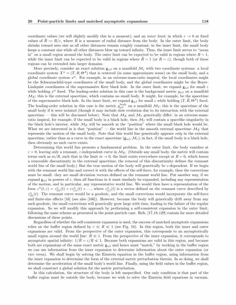
20 Point-particle limits and matched asymptotic expansions 118
coordinate values (we will slightly modify this in a moment); and an inner limit, in which ε → 0 at fixedvalues of R := R/ε, where R is a measure of radial distance from the body. In the outer limit, the bodyshrinks toward zero size as all other distances remain roughly constant; in the inner limit, the small bodykeeps a constant size while all other distances blow up toward infinity. Thus, the inner limit serves to “zoomin” on a small region around the body. The outer limit can be expected to be valid in regions where R ∼ 1,while the inner limit can be expected to be valid in regions where R ∼ 1 (or R ∼ ε), though both of theseregions can be extended into larger domains.
More precisely, consider an exact solution gαβ on a manifold Mε with two coordinate systems: a localcoordinate system Xα = (T,R,ΘA) that is centered (in some approximate sense) on the small body, and aglobal coordinate system xα. For example, in an extreme-mass-ratio inspiral, the local coordinates mightbe the Schwarzschild-type coordinates of the small body, and the global coordinates might be the Boyer-Lindquist coordinates of the supermassive Kerr black hole. In the outer limit, we expand gαβ for small εwhile holding xα fixed. The leading-order solution in this case is the background metric gαβ on a manifoldME ; this is the external spacetime, which contains no small body. It might, for example, be the spacetimeof the supermassive black hole. In the inner limit, we expand gαβ for small ε while holding (T, R,ΘA) fixed.
The leading-order solution in this case is the metric gbodyαβ on a manifold MI ; this is the spacetime of the
small body if it were isolated (though it may include slow evolution due to its interaction with the externalspacetime — this will be discussed below). Note that ME and MI generically differ: in an extreme-mass-ratio inspiral, for example, if the small body is a black hole, then MI will contain a spacelike singularity inthe black hole’s interior, while ME will be smooth at the “position” where the small black hole would be.What we are interested in is that “position” — the world line in the smooth external spacetime ME thatrepresents the motion of the small body. Note that this world line generically appears only in the externalspacetime, rather than as a curve in the exact spacetime (gαβ ,Mε); in fact, if the small body is a black hole,then obviously no such curve exists.
Determining this world line presents a fundamental problem. In the outer limit, the body vanishes atε = 0, leaving only a remnant, ε-independent curve inME . (Outside any small body, the metric will containterms such as m/R, such that in the limit m→ 0, the limit exists everywhere except at R = 0, which leavesa removable discontinuity in the external spacetime; the removal of this discontinuity defines the remnantworld line of the small body.) But the true motion of the body will generically be ε-dependent. If we beginwith the remnant world line and correct it with the effects of the self-force, for example, then the correctionsmust be small: they are small deviation vectors defined on the remnant world line. Put another way, if weexpand gαβ in powers of ε, then all functions in it must similarly be expanded, including any representationof the motion, and in particular, any representative world line. We would then have a representation of theform zα(t, ε) = zα(0)(t) + εzα(1)(t) + . . ., where zα(1)(t) is a vector defined on the remnant curve described by
zα(0)(t). The remnant curve would be a geodesic, and the small corrections would incorporate the self-force
and finite-size effects [16] (see also [166]). However, because the body will generically drift away from anysuch geodesic, the small corrections will generically grow large with time, leading to the failure of the regularexpansion. So we will modify this approach by performing a self-consistent expansion in the outer limit,following the same scheme as presented in the point-particle case. Refs. [17,18,129] contain far more detaileddiscussions of these points.
Regardless of whether the self-consistent expansion is used, the success of matched asymptotic expansionsrelies on the buffer region defined by ε R 1 (see Fig. 10). In this region, both the inner and outerexpansions are valid. From the perspective of the outer expansion, this corresponds to an asymptoticallysmall region around the world line: R 1. From the perspective of the inner expansion, it corresponds toasymptotic spatial infinity: 1/R = ε/R 1. Because both expansions are valid in this region, and becauseboth are expansions of the same exact metric gαβ and hence must “match,” by working in the buffer regionwe can use information from the inner expansion to determine information about the outer expansion (orvice versa). We shall begin by solving the Einstein equation in the buffer region, using information fromthe inner expansion to determine the form of the external metric perturbation therein. In so doing, we shalldetermine the acceleration of the small body’s world line. Finally, using the field values in the buffer region,we shall construct a global solution for the metric perturbation.
In this calculation, the structure of the body is left unspecified. Our only condition is that part of thebuffer region must lie outside the body, because we wish to solve the Einstein field equations in vacuum.
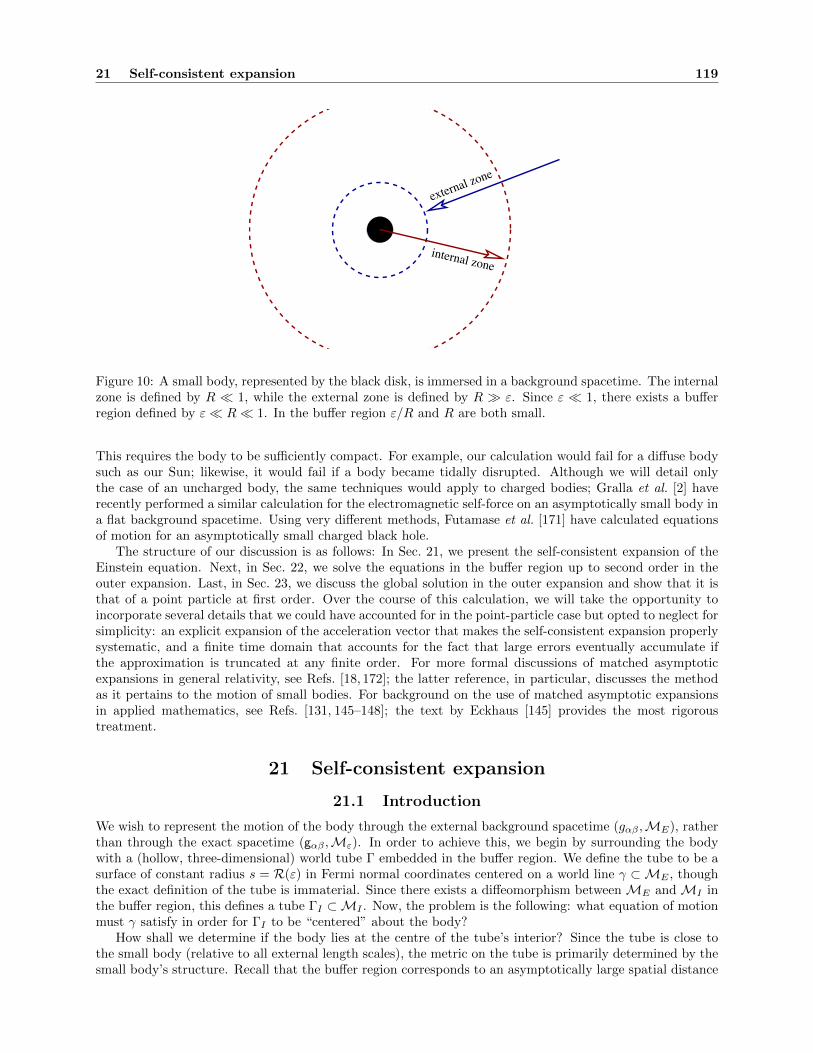
21 Self-consistent expansion 119
internal zone
external zone
Figure 10: A small body, represented by the black disk, is immersed in a background spacetime. The internalzone is defined by R 1, while the external zone is defined by R ε. Since ε 1, there exists a bufferregion defined by ε R 1. In the buffer region ε/R and R are both small.
This requires the body to be sufficiently compact. For example, our calculation would fail for a diffuse bodysuch as our Sun; likewise, it would fail if a body became tidally disrupted. Although we will detail onlythe case of an uncharged body, the same techniques would apply to charged bodies; Gralla et al. [2] haverecently performed a similar calculation for the electromagnetic self-force on an asymptotically small body ina flat background spacetime. Using very different methods, Futamase et al. [171] have calculated equationsof motion for an asymptotically small charged black hole.
The structure of our discussion is as follows: In Sec. 21, we present the self-consistent expansion of theEinstein equation. Next, in Sec. 22, we solve the equations in the buffer region up to second order in theouter expansion. Last, in Sec. 23, we discuss the global solution in the outer expansion and show that it isthat of a point particle at first order. Over the course of this calculation, we will take the opportunity toincorporate several details that we could have accounted for in the point-particle case but opted to neglect forsimplicity: an explicit expansion of the acceleration vector that makes the self-consistent expansion properlysystematic, and a finite time domain that accounts for the fact that large errors eventually accumulate ifthe approximation is truncated at any finite order. For more formal discussions of matched asymptoticexpansions in general relativity, see Refs. [18, 172]; the latter reference, in particular, discusses the methodas it pertains to the motion of small bodies. For background on the use of matched asymptotic expansionsin applied mathematics, see Refs. [131, 145–148]; the text by Eckhaus [145] provides the most rigoroustreatment.
21 Self-consistent expansion
21.1 Introduction
We wish to represent the motion of the body through the external background spacetime (gαβ ,ME), ratherthan through the exact spacetime (gαβ ,Mε). In order to achieve this, we begin by surrounding the bodywith a (hollow, three-dimensional) world tube Γ embedded in the buffer region. We define the tube to be asurface of constant radius s = R(ε) in Fermi normal coordinates centered on a world line γ ⊂ME , thoughthe exact definition of the tube is immaterial. Since there exists a diffeomorphism between ME and MI inthe buffer region, this defines a tube ΓI ⊂MI . Now, the problem is the following: what equation of motionmust γ satisfy in order for ΓI to be “centered” about the body?
How shall we determine if the body lies at the centre of the tube’s interior? Since the tube is close tothe small body (relative to all external length scales), the metric on the tube is primarily determined by thesmall body’s structure. Recall that the buffer region corresponds to an asymptotically large spatial distance
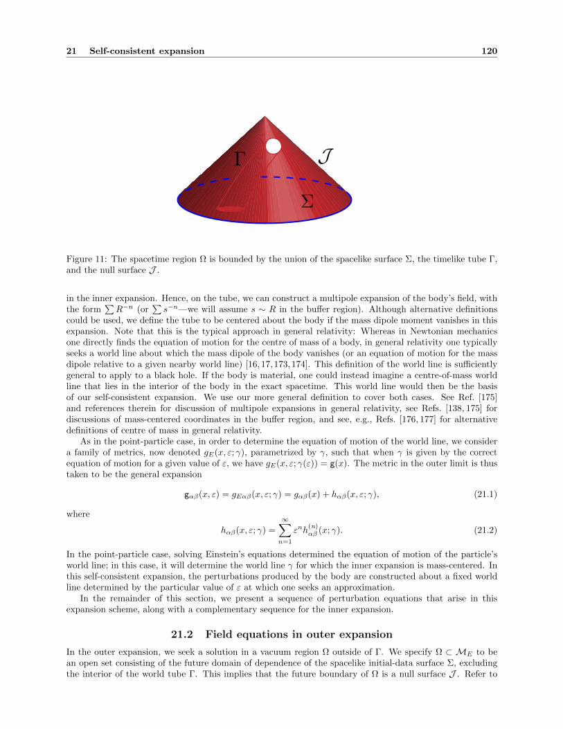
21 Self-consistent expansion 120
Γ
Σ
J
Figure 11: The spacetime region Ω is bounded by the union of the spacelike surface Σ, the timelike tube Γ,and the null surface J .
in the inner expansion. Hence, on the tube, we can construct a multipole expansion of the body’s field, withthe form
∑R−n (or
∑s−n—we will assume s ∼ R in the buffer region). Although alternative definitions
could be used, we define the tube to be centered about the body if the mass dipole moment vanishes in thisexpansion. Note that this is the typical approach in general relativity: Whereas in Newtonian mechanicsone directly finds the equation of motion for the centre of mass of a body, in general relativity one typicallyseeks a world line about which the mass dipole of the body vanishes (or an equation of motion for the massdipole relative to a given nearby world line) [16, 17, 173,174]. This definition of the world line is sufficientlygeneral to apply to a black hole. If the body is material, one could instead imagine a centre-of-mass worldline that lies in the interior of the body in the exact spacetime. This world line would then be the basisof our self-consistent expansion. We use our more general definition to cover both cases. See Ref. [175]and references therein for discussion of multipole expansions in general relativity, see Refs. [138, 175] fordiscussions of mass-centered coordinates in the buffer region, and see, e.g., Refs. [176, 177] for alternativedefinitions of centre of mass in general relativity.
As in the point-particle case, in order to determine the equation of motion of the world line, we considera family of metrics, now denoted gE(x, ε; γ), parametrized by γ, such that when γ is given by the correctequation of motion for a given value of ε, we have gE(x, ε; γ(ε)) = g(x). The metric in the outer limit is thustaken to be the general expansion
gαβ(x, ε) = gEαβ(x, ε; γ) = gαβ(x) + hαβ(x, ε; γ), (21.1)
where
hαβ(x, ε; γ) =
∞∑n=1
εnh(n)αβ (x; γ). (21.2)
In the point-particle case, solving Einstein’s equations determined the equation of motion of the particle’sworld line; in this case, it will determine the world line γ for which the inner expansion is mass-centered. Inthis self-consistent expansion, the perturbations produced by the body are constructed about a fixed worldline determined by the particular value of ε at which one seeks an approximation.
In the remainder of this section, we present a sequence of perturbation equations that arise in thisexpansion scheme, along with a complementary sequence for the inner expansion.
21.2 Field equations in outer expansion
In the outer expansion, we seek a solution in a vacuum region Ω outside of Γ. We specify Ω ⊂ ME to bean open set consisting of the future domain of dependence of the spacelike initial-data surface Σ, excludingthe interior of the world tube Γ. This implies that the future boundary of Ω is a null surface J . Refer to

21 Self-consistent expansion 121
Fig. 11 for an illustration. The boundary of the domain is ∂Ω := Γ∪J ∪Σ. The spatial surface Σ is chosento intersect Γ at the initial time t = 0.
Historically, in derivations of the self-force, solutions to the perturbative field equations were taken tobe global in time, with tail integrals extended to negative infinity, as we wrote them in the precedingsections. But as was first noted in Ref. [17], because the self-force drives long-term, cumulative changes,any approximation truncated at a given order will be accurate to that order only for a finite time; and thisnecessites working in a finite region such as Ω. This is also true in the case of point charges and masses. Forsimplicity, we neglected this detail in the preceding sections, but for completeness, we account for it here.
Field equations
Within this region, we follow the methods presented in the case of a point mass. We begin by reformulatingthe Einstein equation such that it can be solved for an arbitrary world line. To accomplish this, we assumethat the Lorenz gauge can be imposed on the whole of hαβ , everywhere in Ω, such that Lµ[h] = 0. Here
Lµ[h] :=
(gαµg
βν − 1
2gαβg ν
µ
)∇νhαβ (21.3)
is the Lorenz-gauge operator that was first introduced in Secs. 16.1 and 19.1; the condition Lµ[h] = 0 is thesame statement as ∇νγµν = 0, where γµν := hµν − 1
2gµνgαβhαβ is the “trace-reversed” metric perturbation.
We discuss the validity of this assumption below.Just as in the case of a point mass, this choice of gauge reduces the vacuum Einstein equation Rµν = 0
to a weakly nonlinear wave equation that can be expanded and solved at fixed γ. However, we now seeka solution only in the region Ω, where the energy-momentum tensor vanishes, so the resulting sequence ofwave equations reads
Eµν [h(1)] = 0, (21.4)
Eµν [h(2)] = 2δ2Rµν [h(1)], (21.5)
...
whereEµν [h] :=
(gαµg
βν∇γ∇γ + 2R α β
µ ν
)hαβ (21.6)
is the tensorial wave operator that was first introduced in Secs. 16.1 and 19.1, and the second-order Riccitensor δ2Rµν , which is quadratic in its argument, is shown explicitly in Eq (A.1). More generally, we canwrite the nth-order equation as
Eµν[h(n)
]= S(n)
µν
[h(1), . . . , h(n−1), γ
], (21.7)
where the source term S(n)µν consists of nonlinear terms in the expansion of the Ricci tensor.
Again as in the case of a point particle, we can easily write down formal solutions to the wave equations,for arbitrary γ. Using the same methods as were used to derive the Kirchoff representation in Sec. 16.3, wefind
h(n)αβ =
1
4π
∮∂Ω
(G+αβ
γ′δ′∇µ′h(n)γ′δ′ − h
(n)γ′δ′∇µ′G+
αβγ′δ′)dSµ
′+
1
4π
∫Ω
G+αβ
γ′δ′S(n)γ′δ′dV
′. (21.8)
Because J is a future null surface, the integral over it vanishes. Hence, this formal solution requires onlyinitial data on Σ and boundary data on Γ. Since Γ lies in the buffer region, the boundary data on it isdetermined by information from the inner expansion.
One should note several important properties of these integral representations: First, x must lie in theinterior of Ω; an alternative expression must be derived if x lies on the boundary [178]. Second, the integralover the boundary is, in each case, a homogeneous solution to the wave equation, while the integral over thevolume is an inhomogeneous solution. Third, if the field at the boundary satisfies the Lorenz gauge condition,

21 Self-consistent expansion 122
then by virtue of the wave equation, it satisfies the gauge condition everywhere; hence, imposing the gaugecondition to some order in the buffer region ensures that it is imposed to the same order everywhere.
While the integral representation is satisfied by any solution to the associated wave equation, it doesnot provide a solution. That is, one cannot prescribe arbitrary boundary values on Γ and then arrive at asolution. The reason is that the tube is a timelike boundary, which means that field data on it can propagateforward in time and interfere with the data at a later time. However, by applying the wave operator Eαβ onto
equation (21.8), we see that the integral representation of h(n)αβ is guaranteed to satisfy the wave equation
at each point x ∈ Ω. In other words, the problem arises not in satisfying the wave equation in a pointwisesense, but in simultaneously satisfying the boundary conditions. But since the tube is chosen to lie in thebuffer region, these boundary conditions can be supplied by the buffer-region expansion. And as we willdiscuss in Sec. 23, because of the asymptotic smallness of the tube, the pieces of the buffer-region expansiondiverging as s−n are sufficient boundary data to fully determine the global solution.
Finally, just as in the point-particle case, in order to split the gauge condition into a set of exactly solvableequations, we assume that the acceleration of γ possesses an expansion
aµ(t, ε) = aµ(0)(t) + εaµ(1)(t; γ) + . . . . (21.9)
This leads to the set of equations
L(0)µ
[h(1)
]= 0, (21.10)
L(1)µ
[h(1)
]= −L(0)
µ
[h(2)
], (21.11)
...
or, more generally, for n > 0,
L(n)µ
[h(1)
]= −
n∑m=1
L(n−m)µ
[h(m+1)
]. (21.12)
In these expressions, L(0)µ [f ] is the Lorenz-gauge operator acting on the tensor field fαβ evaluated with
aµ = aµ(0), L(1)µ [f ] consists of the terms in Lµ[f ] that are linear in aµ(1), and L
(n)µ [f ] contains the terms linear
in a(n)µ, the combinations a(n−1)µa(1)ν , and so on. Imposing these gauge conditions on the solutions to thewave equations will determine the acceleration of the world line. Although we introduce an expansion of theacceleration vector in order to obtain a systematic sequence of equations that can be solved exactly, such anexpansion also trivially eliminates the need for order-reduction of the resulting equations of motion, since itautomatically leads to equations for a(1)µ in terms of a(0)µ, a(2)µ in terms of a(0)µ and a(1)µ, and so on.
Gauge transformations and the Lorenz condition
The outer expansion is defined not only by holding xα fixed, but also by demanding that the mass dipole of thebody vanishes when calculated in coordinates centered on γ. If we perform a gauge transformation generatedby a vector ξ(1)α(x; γ), then the mass dipole will no longer vanish in those coordinates. Hence, a new worldline γ′ must be constructed, such that the mass dipole vanishes when calculated in coordinates centered onthat new world line. In other words, in the outer expansion we have the usual gauge freedom of regularperturbation theory, so long as the world line is appropriately transformed as well: (hαβ , γ)→ (h′αβ , γ
′). Thetransformation law for the world line was first derived by Barack and Ori [19]; it was displayed in Eq. (1.49),and it will be worked out again in Sec. 22.6.
Using this gauge freedom, we now justify, to some extent, the assumption that the Lorenz gauge conditioncan be imposed on the entirety of hαβ . If we begin with the metric in an arbitrary gauge, then the gaugevectors εξα(1)[γ], ε2ξα(2)[γ], etc., induce the transformation
hαβ → h′αβ = hαβ + ∆hαβ
= hαβ + ε£ξ(1)gαβ + 12ε
2(£ξ(2) + £2ξ(1)
)gαβ + ε2£ξ(1)h(1)αβ +O(ε3). (21.13)
21 Self-consistent expansion 123
If h′αβ is to satisfy the gauge condition Lµ[h′], then ξ must satisfy Lµ[∆h] = −Lµ[h]. After a trivialcalculation, this equation becomes∑
n>0
εn
n!ξα(n) = −εLα
[h(1)
]− ε2Lα
[h(2)
]− ε2Lα
[12£2
ξ(1)g + £ξ(1)h
(1)]
+O(ε3). (21.14)
Solving this equation for arbitrary γ, we equate coefficients of powers of ε, leading to a sequence of waveequations of the form
ξα(n) = Wα(n), (21.15)
where Wα(n) is a functional of ξα(1), . . . , ξ
α(n−1) and h
(1)αβ , . . . , h
(n)αβ . We seek a solution in the region Ω described
in the preceding section. The formal solution reads
ξα(n) = − 1
4π
∫Ω
Gα+α′Wα′
(n)dV′ +
1
4π
∮∂Ω
(Gα+γ′∇µ′ξγ
′
(n) − ξγ′
(n)∇µ′Gα+γ′)dSµ
′. (21.16)
From this we see that the Lorenz gauge condition can be adopted to any desired order of accuracy, giventhe existence of self-consistent data on a tube Γ of asymptotically small radius. We leave the question of thedata’s existence to future work. This argument was first presented in Ref. [18].
21.3 Field equations in inner expansion
For the inner expansion, we assume the existence of some local polar coordinates Xα = (T,R,ΘA), suchthat the metric can be expanded for ε→ 0 while holding fixed R := R/ε, ΘA, and T ; to relate the inner andouter expansions, we assume R ∼ s, but otherwise leave the inner expansion completely general.
This leads to the ansatz
gαβ(T, R,ΘA, ε) = gbodyαβ (T, R,ΘA) +Hαβ(T, R,ΘA, ε), (21.17)
where Hαβ at fixed values of (T, R,ΘA) is a perturbation beginning at order ε. This equation representsan asymptotic expansion along flow lines of constant R/ε as ε → 0. It is tensorial in the usual sense
of perturbation theory: the decomposition into gbodyαβ and Hαβ is valid in any coordinates that can be
decomposed into ε-independent functions of the scaled coordinates plus O(ε) functions of them. As written,
with gbodyαβ depending only on the scaled coordinates and independent of ε, the indices in Eq. (21.17) can
be taken to refer to the unscaled coordinates (T,R,ΘA). However, writing the components in the scaledcoordinates will not alter the form of the expansion, but only introduce an overall rescaling of spatialcomponents due to the spatial forms transforming as, e.g., dR → εdR. For example, if the body is asmall Schwarzschild black hole of ADM mass εm(T ), then in scaled Schwarzschild coordinates (T, R,ΘA),
gbodyαβ (T, R,ΘA) is given by
ds2 = −(1− 2m(T )/R)dT 2 + (1− 2m(T )/R)−1ε2dR2 + ε2R2(dΘ2 + sin ΘdΦ2). (21.18)
As we would expect from the fact that the inner limit follows the body down as it shrinks, all points aremapped to the curve R = 0 at ε = 0, such that the metric in the scaled coordinates naturally becomesone-dimensional at ε = 0. This singular limit can be made regular by rescaling time as well, such thatT = (T − T0)/ε, and then rescaling the entire metric by a conformal factor 1/ε2. In order to arrive at aglobal-in-time inner expansion, rather than a different expansion at each time T0, we forgo this extra step.We do, however, make an equivalent assumption, which is that the metric gbody
αβ and its perturbations arequasistatic (evolving only on timescales ∼ 1). Both approaches are equivalent to assuming that the exactmetric contains no high-frequency oscillations occurring on the body’s natural timescale ∼ ε. In other words,the body is assumed to be in equilibrium. If we did not make this assumption, high-frequency oscillationscould propagate throughout the external spacetime, invalidating our external expansion.
Since we are interested in the inner expansion only insofar as it informs the outer expansion, we shallnot seek to explicitly solve the perturbative Einstein equation in the inner expansion. See Ref. [17] for theforms of the equations and an example of an explicit solution in the case of a perturbed black hole.

22 General expansion in the buffer region 124
22 General expansion in the buffer region
We now seek the general solution to the equations of the outer expansion in the buffer region. To perform theexpansion, we adopt Fermi coordinates centered about γ and expand for small s. In solving the first-orderequations, we will determine a(0)µ; in solving the second-order equations, we will determine a(1)µ, includingthe self-force on the body. Although we perform this calculation in the Lorenz gauge, the choice of gaugeis not essential for our purposes here — the essential aspect is our assumed expansion of the acceleration ofthe world line γ.
22.1 Metric expansions
The method of matched asymptotic expansions relies on the fact that the inner and outer expansion agreeterm by term when re-expanded in the buffer region, where ε s 1. To illustrate this idea of matching,consider the forms of the two expansions in the buffer region. The inner expansion holds s constant (sinceR ∼ s) while expanding for small ε. But if s is replaced with its value s/ε, the inner expansion takes the form
gαβ = gbodyαβ (s/ε)+εH
(1)αβ (s/ε)+· · · , where each term has a dependence on ε that can be expanded in the limit
ε→ 0 to arrive at the schematic forms gbody(s/ε) = 1⊕ε/s⊕ε2/s2⊕ . . . and εH(1)(s/ε) = s⊕ε⊕ε2/s⊕· · · ,where ⊕ signifies “plus terms of the form” and the expanded quantities can be taken to be components inFermi coordinates. Here we have preemptively restricted the form of the expansions, since terms such ass2/ε must vanish because they would have no corresponding terms in the outer expansion. Putting thesetwo expansions together, we arrive at
g(buffer) = 1⊕ ε
s⊕ s⊕ ε⊕ · · · . (22.1)
Since this expansion relies on both an expansion at fixed s and an expansion at fixed s, it can be expectedto be accurate if s 1 and ε s — that is, in the buffer region ε s 1.
On the other hand, the outer expansion holds s constant (since s is formally of the order of the global
external coordinates) while expanding for small ε, leading to the form gαβ = gαβ(s)+εh(1)αβ(s)+ · · · . But very
near the world line, each term in this expansion can be expanded for small s, leading to g = 1⊕ s⊕ s2⊕ · · ·and εh(1) = ε/s⊕ ε⊕ εs⊕ · · · . (Again, we have restricted this form because terms such as ε/s2 cannot arisein the inner expansion.) Putting these two expansions together, we arrive at
g(buffer) = 1⊕ s⊕ ε
s⊕ ε · · · . (22.2)
Since this expansion relies on both an expansion at fixed s and an expansion for small s, it can be expectedto be accurate in the buffer region ε s 1. As we can see, the two buffer-region expansions have anidentical form; and because they are expansions of the same exact metric g, they must agree term by term.
One can make use of this fact by first determining the inner and outer expansions as fully as possible,then fixing any unknown functions in them by matching them term by term in the buffer region; this wasthe route taken in, e.g., Refs. [6, 15, 33, 170]. However, such an approach is complicated by the subtletiesof matching in a diffeomorphism-invariant theory, where the inner and outer expansions are generically indifferent coordinate systems. See Ref. [18] for an analysis of the limitations of this approach as it hastypically been implemented. Alternatively, one can take the opposite approach, working in the buffer regionfirst, constraining the forms of the two expansions by making use of their matching, then using the buffer-region information to construct a global solution; this was the route taken in, e.g., Refs. [16, 17, 166]. Ingeneral, some mixture of these two approaches can be taken. Our calculation follows Ref. [17]. The onlyinformation we take from the inner expansion is its general form, which is characterized by the multipolemoments of the body. From this information, we determine the external expansion, and thence the equationof motion of the world line.
Over the course of our calculation, we will find that the external metric perturbation in the buffer regionis expressed as the sum of two solutions: one that formally diverges at s = 0 and is entirely determinedfrom a combination of (i) the multipole moments of the internal background metric gbody
αβ , (ii) the Riemanntensor of the external background gαβ , and (iii) the acceleration of the world line γ; and a second solutionthat is formally regular at s = 0 and depends on the past history of the body and the initial conditions of
22 General expansion in the buffer region 125
the field. At leading order, these two solutions are identified as the Detweiler-Whiting singular and regularfields hS
αβ and hRαβ , respectively, and the self-force is determined entirely by hR
αβ . Along with the self-force,the acceleration of the world line includes the Papapetrou spin-force [179]. This calculation leaves us withthe self-force in terms of the the metric perturbation in the neighbourhood of the body. In Sec. 23, weuse the local information from the buffer region to construct a global solution for the metric perturbation,completing the solution of the problem.
22.2 The form of the expansion
Before proceeding, we define some notation. We use the multi-index notation ωL := ωi1 · · ·ωi` := ωi1···i` .Angular brackets denote the STF combination of the enclosed indices, and a tensor bearing a hat is an STFtensor. To accomodate this, we now write the Fermi spatial coordinates as xa, instead of xa as they werewritten in previous sections. Finally, we define the one-forms tα := ∂αt and xaα := ∂αx
a.One should note that the coordinate transformation xα(t, xa) between Fermi coordinates and the global
coordinates is ε-dependent, since Fermi coordinates are tethered to an ε-dependent world line. If one wereusing a regular expansion, then this coordinate transformation would devolve into a background coordinatetransformation to a Fermi coordinate system centered on a geodesic world line, combined with a gaugetransformation to account for the ε-dependence. But in the self-consistent expansion, the transformation ispurely a background transformation, because the ε-dependence in it is reducible to that of the fixed worldline.
Because the dependence on ε in the coordinate transformation cannot be reduced to a gauge transfor-mation, in Fermi coordinates the components gαβ of the background metric become ε-dependent. Thisdependence takes the explicit form of factors of the acceleration aµ(t, ε) and its derivatives, for which wehave assumed the expansion ai(t, ε) = a(0)i(t) + a(1)i(t; γ) +O(ε2). There is also an implicit dependence onε in that the proper time t on the world line depends on ε if written as a function of the global coordinates;but this dependence can be ignored so long as we work consistently with Fermi coordinates.
Of course, even in these ε-dependent coordinates, gµν remains the background metric of the outer expan-
sion, and h(n)µν is an exact solution to the wave equation (21.7). At first order we will therefore obtain h
(1)µν
exactly in Fermi coordinates, for arbitrary aµ. However, for some purposes an approximate solution of thewave equation may suffice, in which case we may utilize the expansion of aµ. Substituting that expansion
into gµν and h(n)µν yields the buffer-region expansions
gµν(t, xa; ai) = gµν(t, xa; a(0)i) + εg(1)µν (t, xa; a(1)i) +O(ε2) (22.3)
h(n)µν (t, xa; ai) = h(n)
µν (t, xa; a(0)i) +O(ε), (22.4)
where indices refer to Fermi coordinates, g(1)µν is linear in a(1)i and its derivatives, and for future compactness
of notation we define h(n)Bµν(t, xa) := h
(n)µν (t, xa; a(0)i), where the subscript ‘B’ stands for ‘buffer’. In the case
that a(0)i = 0, these expansions will significantly reduce the complexity of calculations in the buffer region.For that reason, we shall use them in solving the second-order wave equation, but we stress that they aresimply a means of economizing calculations in Fermi coordinates; they do not play a fundamental role in theformalism, and one could readily do without them.
Now, we merely assume that in the buffer region there exists a smooth coordinate transformation betweenthe local coordinates (T,R,ΘA) and the Fermi coordinates (t, xa) such that T ∼ t, R ∼ s, and ΘA ∼ θA.The buffer region corresponds to asymptotic infinity s ε (or s 1) in the internal spacetime. So afterre-expressing s as s/ε, the internal background metric can be expanded as
gbodyαβ (t, s, θA) =
∑n≥0
(εs
)ng
body(n)αβ (t, θA). (22.5)
As mentioned above, since the outer expansion has no negative powers of ε, we exclude them from the inner
expansion. Furthermore, since gαβ + hαβ = gbodyαβ +Hαβ , we must have g
body(0)αβ = gαβ(xa = 0), since these
are the only terms independent of both ε and s. Thus, noting that gαβ(xa = 0) = ηαβ := diag(−1, 1, 1, 1),
22 General expansion in the buffer region 126
we can write
gbodyαβ (t, s, θA) = ηαβ +
ε
sg
body(1)αβ (t, θA) +
(εs
)2
gbody(2)Bαβ (t, θA) +O(ε3/s3), (22.6)
implying that the internal background spacetime is asymptotically flat.We assume that the perturbation Hαβ can be similarly expanded in powers of ε at fixed s,
Hαβ(t, s, θA, ε) = εH(1)αβ (t, s, θA; γ) + ε2H
(2)αβ (t, s, θA; γ) +O(ε3), (22.7)
and that each coefficient can be expanded in powers of 1/s = ε/s to yield
εH(1)αβ (s) = sH
(0,1)αβ + εH
(1,0)αβ +
ε2
sH
(2,−1)αβ +O(ε3/s2), (22.8)
ε2H(2)αβ (s) = s2H
(0,2)αβ + εsH
(1,1)αβ + ε2H
(2,0)αβ + ε2 ln sH
(2,0,ln)αβ +O(ε3/s), (22.9)
ε3H(3)αβ (s) = O(ε3, ε2s, εs2, s3), (22.10)
where H(n,m)αβ , the coefficient of εn and sm, is a function of t and θA (and potentially a functional of γ).
Again, the form of this expansion is constrained by the fact that no negative powers of ε can appear in thebuffer region. (One might think that terms with negative powers of ε could be allowed in the expansion of
gbodyαβ if they are exactly canceled by terms in the expansion of Hαβ , but the differing powers of s in the
two expansions makes this impossible.) Note that explicit powers of s appear because εs = s. Also notethat we allow for a logarithmic term at second order in ε; this term arises because the retarded time in theinternal background includes a logarithmic correction of the form ε ln s (e.g., t− r → t− r∗ in Schwarzschildcoordinates). Since we seek solutions to a wave equation, this correction to the characteristic curves inducesa corresponding correction to the first-order perturbations.
The expansion of Hαβ may or may not hold the acceleration fixed. Regardless of this choice, the generalform of the expansion remains valid: incorporating the expansion of the acceleration would merely shuffleterms from one coefficient to another. And since the internal metric gbody
αβ + Hαβ must equal the external
metric gαβ + hαβ , the general form of the above expansions of gbodyαβ and Hαβ completely determines the
general form of the external perturbations:
h(1)αβ =
1
sh
(1,−1)αβ + h
(1,0)αβ + sh
(1,1)αβ +O(s2), (22.11)
h(2)αβ =
1
s2h
(2,−2)αβ +
1
sh
(2,−1)αβ + h
(2,0)αβ + ln s h
(2,0,ln)αβ +O(s), (22.12)
where each h(n,m)αβ depends only on t and θA, along with an implicit functional dependence on γ. If the
internal expansion is performed with aµ held fixed, then the internal and external quantities are related
order by order: e.g.,∑mH
(0,m)αβ = gαβ , h
(1,−1)αβ = g
body(1)αβ , and h
(1,0)αβ = H
(1,0)αβ . Since we are not concerned
with determining the internal perturbations, the only such relationship of interest is h(n,-n)αβ = g
body(n)αβ . This
equality tells us that the most divergent, s−n piece of the nth-order perturbation h(n)αβ is defined entirely
by the nth-order piece of the internal background metric gbodyαβ , which is the metric of the body if it were
isolated.To obtain a general solution to the Einstein equation, we write each h
(n,m)αβ as an expansion in terms of
irreducible symmetric trace-free pieces:
h(n,m)tt =
∑`≥0
A(n,m)L ωL, (22.13)
h(n,m)ta =
∑`≥0
B(n,m)L ωa
L +∑`≥1
[C
(n,m)aL−1 ω
L−1 + εabcD
(n,m)cL−1 ω
bL−1], (22.14)
h(n,m)ab = δab
∑`≥0
K(n,m)L ωL +
∑`≥0
E(n,m)L ωab
L +∑`≥1
[F
(n,m)L−1〈aωb〉
L−1 + εcd(aωb)cL−1G
(n,m)dL−1
]+∑`≥2
[H
(n,m)abL−2ω
L−2 + εcd(aI(n,m)b)dL−2ωc
L−2]. (22.15)
22 General expansion in the buffer region 127
Here a hat indicates that a tensor is STF with respect to δab, angular brackets 〈〉 indicate the STF combinationof enclosed indices, parentheses indicate the symmetric combination of enclosed indices, and symbols such
as A(n,m)L are functions of time (and potentially functionals of γ) and are STF in all their indices. Each term
in this expansion is linearly independent of all the other terms. All the quantities on the right-hand side areflat-space Cartesian tensors; their indices can be raised or lowered with δab. Refer to Appendix B for moredetails about this expansion.
Now, since the wave equations (21.4) and (21.5) are covariant, they must still hold in the new coordinatesystem, despite the additional ε-dependence. Thus, both equations could be solved for arbitrary accelerationin the buffer region. However, due to the length of the calculations involved, we will instead solve theequations
Eαβ [h(1)] = 0, (22.16)
E(0)αβ [h
(2)B ] = 2δ2R
(0)αβ [h(1)] +O(ε), (22.17)
where E(0)[f ] := E[f ]∣∣a=a(0)
and δ2R(0)[f ] := δ2R[f ]∣∣a=a(0)
. In analogy with the notation used for L(n)µ ,
E(1)µν [f ] and δ2R
(1)µν [f ] would be linear in aµ(1), E
(2)µν [f ] and δ2R
(2)µν [f ] would be linear in aµ(2) and quadratic in
aµ(1), and so on. For a function f ∼ 1, L(n)µ [f ], E
(n)µν [f ], and δ2R
(n)µν [f ] correspond to the coefficients of εn in
expansions in powers of ε. Equation (22.16) is identical to Eq. (21.4). Equation (22.17) follows directly fromsubstituting Eqs. (22.3) and (22.4) into Eq. (21.5); in the buffer region, it captures the dominant behaviour
of h(2)αβ , represented by the approximation h
(2)Bαβ , but it does not capture its full dependence on acceleration.
If one desired a global second-order solution, one might need to solve Eq. (21.5), but for our purpose, whichis to determine the first-order acceleration aµ(1), Eq. (22.17) will suffice.
Unlike the wave equations, the gauge conditions (21.10) and (21.11) already incorporate the expansion ofthe acceleration. As such, they are unmodified by the replacement of the second-order wave equation (21.5)with its approximation (22.17). So we can write
L(0)µ
[h(1)
]= 0, (22.18)
L(1)µ
[h(1)
]= −L(0)
µ
[h
(2)B
], (22.19)
where the first equation is identical to Eq. (21.10), and the second to Eq. (21.11). (The second identity holds
because L(0)µ
[h
(2)B
]= L
(0)µ
[h(2)
], since h
(2)Bαβ differs from h
(2)αβ by aα(1) and higher acceleration terms, which are
set to zero in L(0)µ .) We remind the reader that while this gauge choice is important for finding the external
perturbations globally, any other choice would suffice in the buffer region calculation.In what follows, the reader may safely assume that all calculations are lengthy unless noted otherwise.
22.3 First-order solution in the buffer region
In principle, solving the first-order Einstein equation in the buffer region is straightforward. One need
simply substitute the expansion of h(1)αβ , given in Eq. (22.11), into the linearized wave equation (22.16) and
the gauge condition (22.18). Equating powers of s in the resulting expansions then yields a sequence of
equations that can be solved for successively higher-order terms in h(1)αβ . Solving these equations consists
primarily of expressing each quantity in its irreducible STF form, using the decompositions (B.3) and (B.7);since the terms in this STF decomposition are linearly independent, we can solve each equation term byterm. This calculation is aided by the fact that ∇α = xaα∂a +O(s0), so that, for example, the wave operatorEαβ consists of a flat-space Laplacian ∂a∂a plus corrections of order 1/s. Appendix B also lists many usefulidentities, particularly ∂as = ωa := xa/s, ωa∂aω
L = 0, and the fact that ωL is an eigenvector of the flat-spaceLaplacian: s2∂a∂aω
L = −`(`+ 1)ωL.
Summary of results
Before proceeding with the calculation, which consists mostly of tedious and lengthy algebra, we summarize
the results. The first-order perturbation h(1)αβ consists of two pieces, which we will eventually identify with
22 General expansion in the buffer region 128
the Detweiler-Whiting regular and singular fields. In the buffer-region expansion, the regular field consistsentirely of unknowns, which is to be expected since as a free radiation field, it must be provided by boundarydata. Only when we consider the global solution, in Sec. 23, will we express it in terms of a tail integral.On the other hand, the singular field is locally determined, and it is characterized by the body’s monopolemoment m. More precisely, it is fully determined by the tidal fields of the external background spacetime andthe Arnowitt-Deser-Misner mass of the internal background spacetime gbody
αβ . By itself the wave equationdoes not restrict the behaviour of this monopole moment, but imposing the gauge condition produces theevolution equations
∂tm = 0, ai(0) = 0. (22.20)
Hence, at leading order, the body behaves as a test particle, with constant mass and vanishing acceleration.
Order (1,−1)
We now proceed to the details of the calculation. We begin with the most divergent term in the waveequation: the order 1/s3, flat-space Laplacian term
1
s∂c∂ch
(1,−1)αβ = 0. (22.21)
The tt-component of this equation is
0 = −∑`≥0
`(`+ 1)A(1,−1)L ωL, (22.22)
from which we read off that A(1,−1) is arbitrary and A(1,−1)L must vanish for all ` ≥ 1. The ta-component is
0 = −∑`≥0
(`+ 1)(`+ 2)B(1,−1)L ωa
L −∑`≥1
`(`− 1)C(1,−1)aL−1 ω
L−1
−∑`≥1
`(`+ 1)εabcD(1,−1)cL−1 ωb
L−1, (22.23)
from which we read off that C(1,−1)a is arbitrary and all other coefficients must vanish. Lastly, the ab-
component is
0 = −δab∑`≥0
`(`+ 1)K(1,−1)L ωL −
∑`≥0
(`+ 2)(`+ 3)E(1,−1)L ωab
L
−∑`≥1
`(`+ 1)F(1,−1)L−1〈a ωb〉
L−1 −∑`≥1
(`+ 1)(`+ 2)εcd(aωb)cL−1G
(1,−1)dL−1
−∑`≥2
(`− 2)(`− 1)H(1,−1)abL−2ω
L−2 −∑`≥2
`(`− 1)εcd(aI(1,−1)b)dL−2ωc
L−2, (22.24)
from which we read off that K(1,−1) and H(1,−1)ab are arbitrary and all other coefficients must vanish. Thus,
we find that the wave equation constrains h(1,−1)αβ to be
h(1,−1)αβ = A(1,−1)tαtβ + 2C(1,−1)
a t(βxaα) + (δabK
(1,−1) + H(1,−1)ab )xaαx
bβ . (22.25)
This is further constrained by the most divergent, 1/s2 term in the gauge condition, which reads
− 1
s2h(1,−1)αc ωc +
1
2s2ωαη
µνh(1,−1)µν = 0. (22.26)
From the t-component of this equation, we read off C(1,−1)a = 0; from the a-component, K(1,−1) = A(1,−1)
and H(1,−1)ab = 0. Thus, h
(1,−1)αβ depends only on a single function of time, A(1,−1). By the definition of the

22 General expansion in the buffer region 129
ADM mass, this function (times ε) must be twice the mass of the internal background spacetime. Thus,
h(1,−1)αβ is fully determined to be
h(1,−1)αβ = 2m(t)(tαtβ + δabx
aαx
bβ), (22.27)
where m(t) is defined to be the mass at time t divided by the initial mass ε := m0. (Because the mass willbe found to be a constant, m(t) is merely a placeholder; it is identically unity. We could instead set ε equalto unity at the end of the calculation, in which case m would simply be the mass at time t. Obviously, thedifference between the two approaches is immaterial.)
Order (1, 0)
At the next order, h(1,0)αβ , along with the acceleration of the world line and the time-derivative of the mass,
first appears in the Einstein equation. The order 1/s2 term in the wave equation is
∂c∂ch(1,0)αβ = −2m
s2acω
c(3tαtβ − δabxaαxbβ), (22.28)
where the terms on the right arise from the wave operator acting on s−1h(1,−1)αβ . This equation constrains
h(1,0)αβ to be
h(1,0)tt = A(1,0) + 3macω
c,
h(1,0)ta = C(1,0)
a ,
h(1,0)ab = δab
(K(1,0) −macωc
)+ H
(1,0)ab .
(22.29)
Substituting this result into the order 1/s term in the gauge condition, we find
− 4
stα∂tm+
4m
sa(0)a xaα = 0. (22.30)
Thus, both the leading-order part of the acceleration and the rate of change of the mass of the body vanish:
∂m
∂t= 0 , ai(0) = 0. (22.31)
Order (1, 1)
At the next order, h(1,1)αβ , along with squares and derivatives of the acceleration, first appears in the Einstein
equation, and the tidal fields of the external background couple to s−1h(1,−1)αβ . The order 1/s term in the
wave equation becomes(s∂c∂c +
2
s
)h
(1,1)tt = −20m
3sEijωij −
3m
sa〈iaj〉ω
ij +8m
saia
i, (22.32)(s∂c∂c +
2
s
)h
(1,1)ta = −8m
3sεaijBjkωik −
4m
saa, (22.33)(
s∂c∂c +2
s
)h
(1,1)ab =
20m
9sδabEijωij −
76m
9sEab −
16m
3sE i〈aωb〉i +
8m
sa〈aab〉
+m
sδab(
83aia
i− 3a〈iaj〉ωij). (22.34)
From the tt-component, we read off that A(1,1)i is arbitrary, A(1,1) = 4maia
i, and A(1,1)ij = 5
3mEij + 34ma〈iaj〉;
from the ta-component, B(1,1), C(1,1)ij , and D
(1,1)i are arbitrary, C
(1,1)i = −2mai, and D
(1,1)ij = 2
3mBij ;from the ab component, K
(1,1)i , F
(1,1)i , H
(1,1)ijk , and I
(1,1)ij are arbitrary, and K(1,1) = 4
3maiai, K
(1,1)ij =
− 59mEij + 3
4ma〈iaj〉, F(1,1)ij = 4
3mEij , and H(1,1)ij = − 38
9 mEij + 4ma〈iaj〉.

22 General expansion in the buffer region 130
Substituting this into the order s0 terms in the gauge condition, we find
0 = (ωi + s∂i)h(1,1)αi − 1
2ηµν(ωa − s∂a)h(1,1)
µν xaα − ∂th(1,0)αt − 1
2ηµν∂th
(1,0)µν tα
+ 43mEijωijωα + 2
3mEaiωixaα, (22.35)
where the equation is to be evaluated at ai = ai(0) = 0. From the t-component, we read off
B(1,1) = 16∂t
(A(1,0) + 3K(1,0)
). (22.36)
From the a-component,
F (1,1)a = 3
10
(K(1,1)a − A(1,1)
a + ∂tC(1,0)a
). (22.37)
It is understood that both these equations hold only when evaluated at ai = 0.
Thus, the order s component of h(1)αβ is
h(1,1)tt = 4maia
i + A(1,1)i ωi + 5
3mEijωij + 34ma〈iaj〉ω
ij ,
h(1,1)ta = B(1,1)ωa − 2maa + C
(1,1)ai ωi + εai
jD(1,1)j ωi + 2
3mεaijBjkω
ik,
h(1,1)ab = δab
(43maia
i + K(1,1)i ωi − 5
9mEijωij + 34ma〈iaj〉ω
ij)
+ 43mE i〈aωb〉i
− 389 mEab + 4ma〈aab〉 + H
(1,1)abi ωi + ε ji (aI
(1,1)b)j ωi + F
(1,1)〈a ωb〉.
(22.38)
where B(1,1) and F(1,1)a are constrained to satisfy Eqs. (22.36) and (22.37).
First-order solution
To summarize the results of this section, we have h(1)αβ = s−1h
(1,−1)αβ + h
(1,0)αβ + sh
(1,1)αβ +O(s2), where h
(1,−1)αβ
is given in Eq. (22.27), h(1,0)αβ is given in Eq. (22.29), and h
(1,1)αβ is given in Eq. (22.38). In addition, we have
determined that the ADM mass of the internal background spacetime is time-independent, and that theacceleration of the body’s world line vanishes at leading order.
22.4 Second-order solution in the buffer region
Though the calculations are much lengthier, solving the second-order Einstein equation in the buffer region isessentially no different from solving the first. We seek to solve the approximate wave equation (22.17), along
with the gauge condition (22.19), for the second-order perturbation h(2)Bαβ := h
(2)αβ
∣∣a=a0
; doing so will also,
more importantly, determine the acceleration aµ(1). In this calculation, the acceleration is set to ai = ai(0) = 0
everywhere except in the left-hand side of the gauge condition, L(1)µ [h(1)], which is linear in aµ(1).
Summary of results
We first summarize the results. As at first order, the metric perturbation contains a regular, free radiationfield and a singular, bound field; but in addition to these pieces, it also contains terms sourced by the first-order perturbation. Again, the regular field requires boundary data to be fully determined. And again, thesingular field is characterized by the multipole moments of the body: the mass dipole Mi of the internalbackground metric gbody
αβ , which measures the shift of the body’s centre of mass relative to the world line;
the spin dipole Si of gbodyαβ , which measures the spin of the body about the world line; and an effective
correction δm to the body’s mass. The wave equation by itself imposes no restriction on these quantities,but by imposing the gauge condition we find the evolution equations
∂tδm =m
3∂tA
(1,0) +5m
6∂tK
(1,0), (22.39)
∂tSa = 0, (22.40)
∂2tMa + EabM b = −a(1)
a + 12 A
(1,1)a − ∂tC(1,0)
a − 1
mSiBia. (22.41)
22 General expansion in the buffer region 131
The first of these tells us that the free radiation field created by the body creates a time-varying shift in thebody’s mass. We can immediately integrate it to find
δm(t) = δm(0) + 16m[2A(1,0)(t) + 5K(1,0)(t)
]− 1
6m[2A(1,0)(0) + 5K(1,0)(0)
]. (22.42)
We note that this mass correction is entirely gauge dependent; it could be removed by redefining the timecoordinate on the world line. In addition, one could choose to incorporate δm(0) into the leading-order massm. The second of the equations tells us that the body’s spin is constant at this order; at higher orders,time-dependent corrections to the spin dipole would arise. The last of the equations is the principal resultof this section. It tells us that the relationship between the acceleration of the world line and the drift ofthe body away from it is governed by (i) the local curvature of the background spacetime, as characterizedby Eab — this is the same term that appears in the geodesic deviation equation — (ii) the coupling of thebody’s spin to the local curvature — this is the Papapetrou spin force [179] — and (iii) the free radiationfield created by the body — this is the self-force. We identify the world line as the body’s by the conditionMi = 0. If we start with initial conditions Mi(0) = 0 = ∂tMi(0), then the mass dipole remains zero for alltimes if and only if the world line satisfies the equation
a(1)a = 1
2 A(1,1)a − ∂tC(1,0)
a − 1
mSiBia. (22.43)
This is the equation of motion we sought. It, along with the more general equation containing Mi, will bediscussed further in the following section.
Order (2,−2)
We now proceed to the details of the calculation. Substituting the expansion
h(2)αβ =
1
s2h
(2,−2)Bαβ +
1
sh
(2,−1)Bαβ + h
(2,0)Bαβ + ln(s)h
(2,0,ln)Bαβ +O(ε, s) (22.44)
and the results for h(1)αβ from the previous section into the wave equation and the gauge condition again
yields a sequence of equations that can be solved for coefficients of successively higher-order powers (andlogarithms) of s. Due to its length, the expansion of the second-order Ricci tensor is given in Appendix A.
Note that since the approximate wave equation (22.17) contains an explicit O(ε) correction, h(2)αβ will be
determined only up to O(ε) corrections. For simplicity, we omit these O(ε) symbols from the equations inthis section; note, however, that these corrections do not effect the gauge condition, as discussed above.
To begin, the most divergent, order 1/s4 term in the wave equation reads
1
s4
(2 + s2∂c∂c
)h
(2,−2)Bαβ =
4m2
s4
(7ωab + 4
3δab)xaαx
bβ −
4m2
s4tαtβ , (22.45)
where the right-hand side is the most divergent part of the second-order Ricci tensor, as given in Eq. (A.3).
From the tt-component of this equation, we read off A(2,−2) = −2m2 and that A(2,−2)a is arbitrary. From
the ta-component, B(2,−2), C(2,−2)ab , and D
(2,−2)c are arbitrary. From the ab-component, K(2,−2) = 8
3m2,
E(2,−2) = −7m2, and K(2,−2)a , F
(2,−2)a , H
(2,−2)abc , and I
(2,−2)ab are arbitrary.
The most divergent, order 1/s3 terms in the gauge condition similarly involve only h(2,−2)αβ ; they read
1
s3
(s∂b − 2ωb
)h
(2,−2)Bαb − 1
2s3ηµνxaα (s∂a − 2ωa)h
(2,−2)Bµν = 0. (22.46)
After substituting the results from the wave equation, the t-component of this equation determines that
C(2,−2)ab = 0. The a-component determines that H
(2,−2)abc = 0, I
(2,−2)ab = 0, and
F (2,−2)a = 3K(2,−2)
a − 3A(2,−2)a . (22.47)
22 General expansion in the buffer region 132
Thus, the order 1/s2 part of h(2)αβ is given by
h(2,−2)Btt = −2m2 + A
(2,−2)i ωi,
h(2,−2)Bta = B(2,−2)ωa + εa
ijωiD(2,−2)j ,
h(2,−2)Bab = δab
(83m
2 + K(2,−2)i ωi
)− 7m2ωab + F
(2,−2)〈a ωb〉,
(22.48)
where F(2,−2)a is given by Eq. (22.47).
The metric perturbation in this form depends on five free functions of time. However, from calculationsin flat spacetime, we know that order ε2/s2 terms in the metric perturbation can be written in terms oftwo free functions: a mass dipole and a spin dipole. We transform the perturbation into this “canonical”form by performing a gauge transformation (c.f. Ref. [180]). The transformation is generated by ξα =
− 1s B
(2,−2)tα − 12s F
(2,−2)a xaα, the effect of which is to remove B(2,−2) and F
(2,−2)a from the metric. This
transformation is a refinement of the Lorenz gauge. (Effects at higher order in ε and s will be automatically
incorporated into the higher-order perturbations.) The condition F(2,−2)a − 3K
(2,−2)a + 3A
(2,−2)a = 0 then
becomes K(2,−2)a = A
(2,−2)a . The remaining two functions are related to the ADM momenta of the internal
spacetime:
A(2,−2)i = 2Mi , D
(2,−2)i = 2Si, (22.49)
where Mi is such that ∂tMi is proportional to the ADM linear momentum of the internal spacetime, and Siis the ADM angular momentum. Mi is a mass dipole term; it is what would result from a transformation
xa → xa + Ma/m applied to the 1/s term in h(1)αβ . Si is a spin dipole term. Thus, the order 1/s2 part of
h(2)Bαβ reads
h(2,−2)Btt = −2m2 + 2Miω
i,
h(2,−2)Bta = 2εaijω
iSj ,
h(2,−2)Bab = δab
(83m
2 + 2Miωi)− 7m2ωab.
(22.50)
Order (2,−1)
At the next order, 1/s3, because the acceleration is set to zero, h(2,−2)Bαβ does not contribute to E
(0)µν [h(2)], and
h(1,−1)Bαβ does not contribute to δ2R
(0)µν [h(1)]. The wave equation hence reads
1
s∂c∂ch
(2,−1)Bαβ =
2
s3δ2R
(0,−3)αβ
[h(1)
], (22.51)
where δ2R(0,−3)αβ
[h(1)
]is given in Eqs. (A.4)–(A.6). The tt-component of this equation implies s2∂c∂ch
(2,−1)Btt =
6mH(1,0)ij ωij , from which we read off that A(2,−1) is arbitrary and A
(2,−1)ij = −mH(1,0)
ij . The ta-component
implies s2∂c∂ch(2,−1)Bta = 6mC
(1,0)i ωia, from which we read off B
(2,−1)i = −mC(1,0)
i and that C(2,−1)a is arbitrary.
The ab-component implies
s2∂c∂ch(2,−1)Bab = 6m
(A(1,0) + K(1,0)
)ωab − 12mH
(1,0)i〈a ωb〉
i + 2mδabH(1,0)ij ωij , (22.52)
from which we read off that K(2,−1) is arbitrary, K(2,−1)ij = − 1
3mH(1,0)ij , E(2,−1) = −mA(1,0) − mK(1,0),
F(2,−1)ab = 2mH
(1,0)ab , and H
(2,−1)ab is arbitrary. This restricts h
(2,−1)αβ to the form
h(2,−1)Btt = A(2,−1) −mH(1,0)
ij ωij ,
h(2,−1)Bta = −mC(1,0)
i ωia + C(2,−1)a ,
h(2,−1)Bab = δab
(K(2,−1) − 1
3mH(1,0)ij ωij
)−m
(A(1,0) + K(1,0)
)ωab + 2mH
(1,0)i〈a ωb〉
i + H(2,−1)ab .
(22.53)

22 General expansion in the buffer region 133
We next substitute h(2,−2)Bαβ and h
(2,−1)Bαβ into the order 1/s2 terms in the gauge condition. The t-component
becomes1
s2
(4mC
(1,0)i + 12∂tMi + 3C
(2,−1)i
)ωi = 0, (22.54)
from which we read offC
(2,−1)i = −4∂tMi − 4
3mC(1,0)i . (22.55)
And the a-component becomes
0 =(− 4
3mA(1,0) − 4
3mK(1,0) − 1
2 A(2,−1) + 1
2K(2,−1)
)ωa +
(23mH
(1,0)ai − H(2,−1)
ai
)ωi
− 2εijaωi∂tS
j , (22.56)
from which we read off
A(2,−1) = K(2,−1) − 83m(A(1,0) + K(1,0)
), (22.57)
H(2,−1)ij = 2
3mH(1,0)ij , (22.58)
and that the angular momentum of the internal background is constant at leading order:
∂tSi = 0. (22.59)
Thus, the order 1/s term in h(2)Bαβ is given by
h(2,−1)Btt = K(2,−1) − 8
3m(A(1,0) + K(1,0)
)−mH(1,0)
ij ωij ,
h(2,−1)Bta = −mC(1,0)
i ωia − 4∂tMi − 43mC
(2,−1)i ,
h(2,−1)Bab = δab
(K(2,−1) − 1
3mH(1,0)ij ωij
)−m
(A(1,0) + K(1,0)
)ωab + 2mH
(1,0)i〈a ωb〉
i + 23mH
(1,0)ab .
(22.60)
Note that the undetermined function K(2,−1) appears in precisely the form of a mass monopole. The value ofthis function will never be determined (though its time-dependence will be). This ambiguity arises becausethe mass m that we have defined is the mass of the internal background spacetime, which is based on theinner limit that holds ε/R fixed. A term of the form ε2/R appears as a perturbation of this background,even when, as in this case, it is part of the mass monopole of the body. This is equivalent to the ambiguityin any expansion in one’s choice of small parameter: one could expand in powers of ε, or one could expand inpowers of ε+ε2, and so on. It is also equivalent to the ambiguity in defining the mass of a non-isolated body;whether the “mass” of the body is taken to be m or m+ 1
2K(2,−1) is a matter of taste. As we shall discover,
the time-dependent part of K(2,−1) is constructed from the tail terms in the first-order metric perturbation.Hence, the ambiguity in the definition of the mass is, at least in part, equivalent to whether or not onechooses to include the free gravitational field induced by the body in what one calls its mass. (In fact, anyorder ε incoming radiation, not just that originally produced by the body, will contribute to this effectivemass.) In any case, we will define the “correction” to the mass as δm := 1
2K(2,−1).
Order (2, 0, ln)
We next move to the order ln(s)/s2 terms in the wave equation, and the order ln(s)/s terms in the gaugecondition, which read
ln s∂c∂ch(2,0,ln)Bαβ = 0, (22.61)
ln s(∂bh
(2,0,ln)Bαb − 1
2ηµνxaα∂ah
(2,0,ln)Bµν
)= 0. (22.62)
From this we determine
h(2,0,ln)Bαβ = A(2,0,ln)tαtβ + 2C(2,0,ln)
a t(βxaα) + (δabK
(2,0,ln) + H(2,0,ln)ab )xaαx
bβ . (22.63)

22 General expansion in the buffer region 134
Finally, we arrive at the order 1/s2 terms in the wave equation. At this order, the body’s tidal momentsbecome coupled to those of the external background. The equation reads
∂c∂ch(2,0)Bαβ +
1
s2
(h
(2,0,ln)Bαβ + Eαβ
)=
2
s2δ2R
(0,−2)αβ
[h
(1)B
], (22.64)
where Eαβ comprises the contributions from h(2,−2)Bαβ and h
(2,−1)Bαβ , given in Eqs. (A.10), (A.15), and (A.21).
The contribution from the second-order Ricci tensor is given in Eqs. (A.7)–(A.9).Foregoing the details, after some algebra we can read off the solution
h(2,0)Btt = A(2,0) + A
(2,0)i ωi + A
(2,0)ij ωij + A
(2,0)ijk ωijk (22.65)
h(2,0)Bta = B(2,0)ωa + B
(2,0)ij ωa
ij + C(2,0)a + C
(2,0)ai ωa
i + εabc(D(2,0)c ωb + D
(2,0)ci ωb
i + D(2,0)cij ωb
ij)
(22.66)
h(2,0)Bab = δab
(K(2,0) + K
(2,0)i ωi + K
(2,0)ijk ωijk
)+ E
(2,0)i ωab
i + E(2,0)ij ωab
ij + F(2,0)〈a ωb〉 + F
(2,0)i〈a ωb〉
i
+ F(2,0)ij〈a ωb〉
ij + εcd(aωb)ciG
(2,0)di + H
(2,0)ab + H
(2,0)abi ωi + εcd(aI
(2,0)b)d ωc, (22.67)
where each one of the STF tensors is listed in Table 1.In solving Eq. (22.64), we also find that the logarithmic term in the expansion becomes uniquely deter-
mined:h
(2,0,ln)Bαβ = − 16
15m2Eabxaαxbβ . (22.68)
This term arises because the sources in the wave equation (22.64) contain a term ∝ Eab, which cannot
be equated to any term in ∂c∂ch(2,0)Bab . Thus, the wave equation cannot be satisfied without including a
logarithmic term.
Gauge condition
We now move to the final equation in the buffer region: the order 1/s gauge condition. This condition will
determine the acceleration aα(1). At this order, h(1)αβ first contributes to Eq. (22.19):
L(1,−1)α [h(1)] =
4m
sa(1)a xaα. (22.69)
The contribution from h(2)Bαβ is most easily calculated by making use of Eqs. (B.24) and (B.25). After some
algebra, we find that the t-component of the gauge condition reduces to
0 = −4
s∂tδm+
4m
3s∂tA
(1,0) +10m
3s∂tK
(1,0), (22.70)
and the a-component reduces to
0 =4
s∂2tMa +
4m
sa(1)a +
4
sEaiM i +
4
sBaiSi −
2m
sA(1,1)a +
4m
s∂tC
(1,0)a . (22.71)
After removing common factors, these equations become Eqs. (22.39) and (22.41). We remind the reader
that these equations are valid only when evaluated at aa(t) = aa(0)(t) = 0, except in the term 4ma(1)a /s that
arose from L(1)α [h(1)].
Second-order solution
We have now completed our calculation in the buffer region. In summary, the second-order perturbation in
the buffer region is given by h(2)αβ = s−2h
(2,−2)Bαβ + s−1h
(2,−1)Bαβ + h
(2,0)Bαβ + ln(s)h
(2,0,ln)Bαβ + O(ε, s), where h
(2,−2)Bαβ
is given in Eq. (22.50), h(2,−1)Bαβ in Eq. (22.60), h
(2,0)Bαβ in Eq. (22.65), and h
(2,0,ln)Bαβ in Eq. (22.68). In addition,
we have found evolution equations for an effective correction to the body’s mass, given by Eq. (22.39), andmass and spin dipoles, given by Eqs. (22.59) and (22.71).
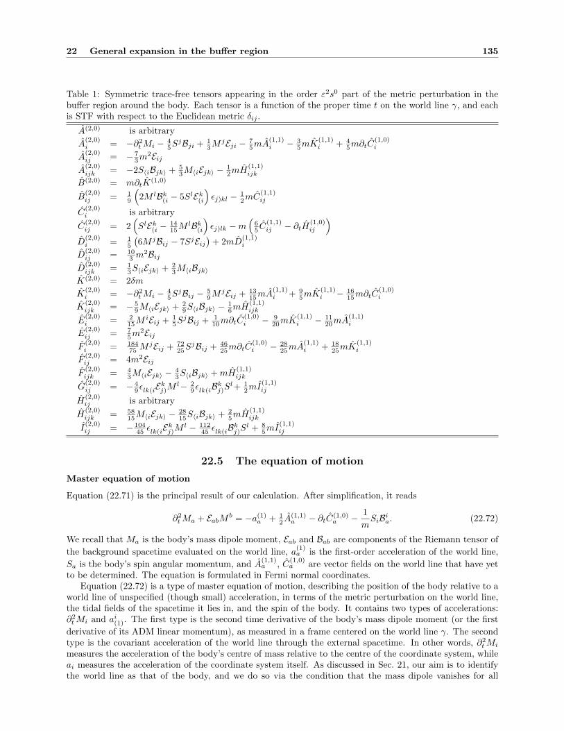
22 General expansion in the buffer region 135
Table 1: Symmetric trace-free tensors appearing in the order ε2s0 part of the metric perturbation in thebuffer region around the body. Each tensor is a function of the proper time t on the world line γ, and eachis STF with respect to the Euclidean metric δij .
A(2,0) is arbitrary
A(2,0)i = −∂2
tMi − 45S
jBji + 13M
jEji − 75mA
(1,1)i − 3
5mK(1,1)i + 4
5m∂tC(1,0)i
A(2,0)ij = − 7
3m2Eij
A(2,0)ijk = −2S〈iBjk〉 + 5
3M〈iEjk〉 − 12mH
(1,1)ijk
B(2,0) = m∂tK(1,0)
B(2,0)ij = 1
9
(2M lBk(i − 5SlEk(i
)εj)kl − 1
2mC(1,1)ij
C(2,0)i is arbitrary
C(2,0)ij = 2
(SlEk(i − 14
15MlBk(i
)εj)lk −m
(65 C
(1,1)ij − ∂tH(1,0)
ij
)D
(2,0)i = 1
5
(6M jBij − 7SjEij
)+ 2mD
(1,1)i
D(2,0)ij = 10
3 m2Bij
D(2,0)ijk = 1
3S〈iEjk〉 + 23M〈iBjk〉
K(2,0) = 2δm
K(2,0)i = −∂2
tMi − 45S
jBij − 59M
jEij + 1315mA
(1,1)i + 9
5mK(1,1)i − 16
15m∂tC(1,0)i
K(2,0)ijk = − 5
9M〈iEjk〉 + 29S〈iBjk〉 − 1
6mH(1,1)ijk
E(2,0)i = 2
15MiEij + 1
5SjBij + 1
10m∂tC(1,0)i − 9
20mK(1,1)i − 11
20mA(1,1)i
E(2,0)ij = 7
5m2Eij
F(2,0)i = 184
75 MjEij + 72
25SjBij + 46
25m∂tC(1,0)i − 28
25mA(1,1)i + 18
25mK(1,1)i
F(2,0)ij = 4m2EijF
(2,0)ijk = 4
3M〈iEjk〉 − 43S〈iBjk〉 +mH
(1,1)ijk
G(2,0)ij = − 4
9εlk(iEkj)M l− 29εlk(iBkj)Sl+ 1
2mI(1,1)ij
H(2,0)ij is arbitrary
H(2,0)ijk = 58
15M〈iEjk〉 − 2815S〈iBjk〉 + 2
5mH(1,1)ijk
I(2,0)ij = − 104
45 εlk(iEkj)M l − 11245 εlk(iBkj)Sl + 8
5mI(1,1)ij
22.5 The equation of motion
Master equation of motion
Equation (22.71) is the principal result of our calculation. After simplification, it reads
∂2tMa + EabM b = −a(1)
a + 12 A
(1,1)a − ∂tC(1,0)
a − 1
mSiBia. (22.72)
We recall that Ma is the body’s mass dipole moment, Eab and Bab are components of the Riemann tensor of
the background spacetime evaluated on the world line, a(1)a is the first-order acceleration of the world line,
Sa is the body’s spin angular momentum, and A(1,1)a , C
(1,0)a are vector fields on the world line that have yet
to be determined. The equation is formulated in Fermi normal coordinates.Equation (22.72) is a type of master equation of motion, describing the position of the body relative to a
world line of unspecified (though small) acceleration, in terms of the metric perturbation on the world line,the tidal fields of the spacetime it lies in, and the spin of the body. It contains two types of accelerations:∂2tMi and ai(1). The first type is the second time derivative of the body’s mass dipole moment (or the first
derivative of its ADM linear momentum), as measured in a frame centered on the world line γ. The secondtype is the covariant acceleration of the world line through the external spacetime. In other words, ∂2
tMi
measures the acceleration of the body’s centre of mass relative to the centre of the coordinate system, whileai measures the acceleration of the coordinate system itself. As discussed in Sec. 21, our aim is to identifythe world line as that of the body, and we do so via the condition that the mass dipole vanishes for all
22 General expansion in the buffer region 136
times, meaning that the body is centered on the world line for all times. If we start with initial conditionsMi(0) = 0 = ∂tMi(0), then the mass dipole remains zero for all times if and only if the world line satisfiesthe equation
a(1)a = 1
2 A(1,1)a − ∂tC(1,0)
a − 1
mSiBia. (22.73)
This equation of motion contains two types of terms: a Papapetrou spin force, given by −SiBia, which arisesdue to the coupling of the body’s spin to the local magnetic-type tidal field of the external spacetime; and aself-force, arising from homogenous terms in the wave equation. Note that the right-hand side of this equationis to be evaluated at aµ = a(0)µ = 0, and that it would contain an antidamping term − 11
3 maµ [7,149,150] if
we had not assumed that the acceleration possesses an expansion of the form given in Eq. (21.9).In our self-consistent approach, we began with the aim of identifying γ by the condition that the body
must be centered about it for all time. However, we could have begun with a regular expansion, in whichthe world line is taken to be the remnant γ(0) of the body in the outer limit of ε → 0 with only xµ fixed.In that case the acceleration of the world line would necessarily be ε-independent, so ai(0) would be the full
acceleration of γ(0). Hence, when we found ai(0) = 0, we would have identified the world line as a geodesic,
and there would be no corrections ai(n) for n > 0. We would then have arrived at the equation of motion
∂2tMa + EabM b = 1
2 A(1,1)a − ∂tC(1,0)
a − 1
mSiBia. (22.74)
This equation of motion was first derived by Gralla and Wald [16] (although they phrased their expansion interms of an explicit expansion of the world line, with a deviation vector on γ(0), rather than the mass dipole,measuring the correction to the motion). It describes the drift of the body away from the reference geodesicγ(0). This drift is driven partially by the local curvature of the background, as seen in the geodesic-deviationterm EabM b, and by the coupling between the body’s spin and the local curvature. It is also driven by the
self-force, as seen in the terms containing A(1,1)a and C
(1,0)a , but unlike in the self-consistent equation, the
fields that produce the self-force are generated by a geodesic past history (plus free propagation from initialdata) rather than by the corrected motion.
Although perfectly valid, such an equation is of limited use. If the external background is curved, thenMi has meaning only if the body is “close” to the world line. Thus, ∂2
tMi is a meaningful accelerationonly for a short time, since Mi will generically grow large as the body drifts away from the reference worldline. On that short timescale of validity, the deviation vector defined by M i accurately points from γ(0)
to a “corrected” world line γ; that world line, the approximate equation of motion of which is given inEq. (22.73), accurately tracks the motion of the body. After a short time, when the mass dipole grows largeand the regular expansion scheme begins to break down, the deviation vector will no longer correctly pointto the corrected world line. Errors will also accumulate in the field itself, because it is being sourced by thegeodesic, rather than corrected, motion.
The self-consistent equation of motion appears to be more robust, and offers a much wider range ofvalidity. Furthermore, even beyond the above step, where we had the option to choose to set either Mi
or ai(0) to zero, the self-consistent expansion continues to contain within it the regular expansion. Startingfrom the solution in the self-consistent expansion, one can recover the regular expansion, and its equation ofmotion (22.74), simply by assuming an expansion for the world line and following the usual steps of derivingthe geodesic deviation equation.
Detweiler-Whiting decomposition
Regardless of which equation of motion we opt to use, we have now completed the derivation of the grav-itational self-force, in the sense that, given the metric perturbation in the neighbourhood of the body, theself-force is uniquely determined by irreducible pieces of that perturbation. Explicitly, the terms that appearin the self-force are given by
A(1,1)a =
3
4π
∫ωah
(1,1)tt dΩ, (22.75)
C(1,0)a = h
(1,0)ta . (22.76)

22 General expansion in the buffer region 137
This is all that is needed to incorporate the motion of the body into a dynamical system that can benumerically evolved; at each timestep, one simply needs to calculate the field near the world line anddecompose it into irreducible pieces in order to determine the acceleration of the body. The remainingdifficulty is to actually determine the field at each timestep. In the next section, we will use the formalintegral representation of the solution to determine the metric perturbation at the location of the body interms of a tail integral.
However, before doing so, we emphasize some important features of the self-force and the field near the
body. First, note that the first-order external field h(1)αβ splits into two distinct pieces. There is the singular
piece hSαβ , given by
hStt =
2m
s
1 + 3
2saiωi + 2s2aia
i + s2(
38a〈iaj〉 + 5
6Eij)ωij
+O(s2) (22.77)
hSta = −2msaa + 2
3msεaijBjkω
ik +O(s2) (22.78)
hSab =
2m
s
δab[1− 1
2saiωi + 2
3s2aia
i + s2(
38a〈iaj〉 − 5
18Eij)ωij]
+ 2s2a〈aab〉
− 199 s
2Eab + 23s
2E i〈aωb〉i
+O(s2). (22.79)
This field is a solution to the homogenous wave equation for s > 0, but it is divergent at s = 0. It isthe generalization of the 1/s Newtonian field of the body, as perturbed by the tidal fields of the externalspacetime gαβ . Comparing with results to be derived below in Sec. 23.2, we find that it is precisely theDetweiler-Whiting singular field for a point mass.
Next, there is the Detweiler-Whiting regular field hRαβ = h
(1)αβ − hS
αβ , given by
hRtt = A(1,0) + sA
(1,1)i ωi +O(s2), (22.80)
hRta = C(1,0)
a + s(B(1,1)ωa + C
(1,1)ai ωi + εai
jD(1,1)j ωi
)+O(s2), (22.81)
hRab = δabK
(1,0) + H(1,0)ab + s
(δabK
(1,1)i ωi + H
(1,1)abi ωi + ε ji (aI
(1,1)b)j ωi + F
(1,1)〈a ωb〉
)+O(s2). (22.82)
This field is a solution to the homogeneous wave equation even at s = 0. It is a free radiation field in theneighbourhood of the body. And it contains all the free functions in the buffer-region expansion.
Now, the acceleration of the body is given by
a(1)a = 1
2∂ahRtt − ∂thR
ta −1
mSiBia, (22.83)
which we can rewrite as
aα(1) = − 12
(gαδ + uαuδ
)(2hR
δβ;γ − hRβγ;δ
)∣∣a=0
uβuγ +1
2mRαβγδu
βSγδ, (22.84)
where Sγδ := eγc eδdεcdjSj . In other words, up to order ε2 errors, a body with order ε or smaller spin (i.e., one
for which Sγδ = 0), moves on a geodesic of a spacetime gαβ + εhRαβ , where hR
αβ is a free radiation field in theneighbourhood of the body; a local observer would measure the “background spacetime,” in which the bodyis in free fall, to have the metric gαβ + εhRαβ instead of gαβ . If we performed a transformation into Fermi
coordinates in gαβ + εhRαβ , the metric would contain no acceleration term, and it would take the simple formof a smooth background plus a singular perturbation. Hence, the Detweiler-Whiting axiom is a consequence,rather than an assumption, of our derivation, and we have recovered precisely the picture it provides in thepoint particle case. In the electromagnetic and scalar cases, Harte has shown that this result is quite general:even for a finite extended body, the field it produces can be split into a homogeneous field [157,158,181] thatexerts a direct force on the body, and a nonhomogeneous field that exerts only an indirect force by alteringthe body’s multipole moments. His results should be generalizable to the gravitational case as well.

22 General expansion in the buffer region 138
22.6 The effect of a gauge transformation on the force
We now turn to the question of how the world line transforms under a gauge transformation. We begin withthe equation of motion (22.41), presented again here:
∂2tMa + EaiM i = −a(1)
a −1
mBaiSi +
[12 A
(1,1)a − ∂tC(1,0)
a
]aµ=0
. (22.85)
Setting Mi = 0, we derive the first-order acceleration of γ, given in Eq. (22.73). If, for simplicity, we neglectthe Papapetrou spin term, then that acceleration is given by
a(1)a = lim
s→0
(3
4π
∫ωa2sh
(1)tt dΩ− ∂th(1)
ta
)= lims→0
3
4π
∫ (12∂ih
(1)tt − ∂th(1)
ti
)ωiωadΩ, (22.86)
where it is understood that explicit appearances of the acceleration are to be set to zero on the right-
hand side. The first equality follows directly from Eq. (22.73) and the definitions of A(1,1)a and C
(1,0)a .
The second equality follows from the STF decomposition of h(1)αβ and the integral identities (B.26)–(B.28).
We could also readily derive the form of the force given by the Quinn-Wald method of regularization:
lims→01
4π
∫ (12∂ah
(1)tt − ∂th(1)
ta
)dΩ. However, in order to derive a gauge-invariant equation of motion, we
shall use the form in Eq. (22.86).Suppose that we had not chosen a world line for which the mass dipole vanishes, but instead had chosen
some “nearby” world line. Then Eq. (22.85) provides the relationship between the acceleration of thatworld line, the mass dipole relative to it, and the first-order metric perturbations (we again neglect spin for
simplicity). The mass dipole is given by Mi = 38π lims→0
∫s2h
(2)tt ωidΩ, which has the covariant form
Mα′ =3
8πlims→0
∫gαα′ωαs
2h(2)µν u
µuνdΩ, (22.87)
where a primed index corresponds to a point on the world line. Note that the parallel propagator does notinterfere with the angle-averaging, because in Fermi coordinates, gαβ′ = δαβ + O(ε, s2). One can also rewritethe first-order-metric-perturbation terms in Eq. (22.85) using the form given in Eq. (22.86). We then haveEq. (22.85) in the covariant form
3
8πlims→0
∫gαα′
(gαβ
D2
dτ2+ Eαβ
)ωβs2h(2)
µν uµuνdΩ
∣∣a=a(0)
= −3m
8πlims→0
∫gαα′(
2h(1)βµ;ν − h
(1)µν;β
)uµuνωβαdΩ
∣∣a=a(0)
−ma(1)α′ . (22.88)
Now consider a gauge transformation generated by εξ(1)α[γ] + 12ε
2ξ(2)α[γ] + · · · , where ξ(1)α is bounded
as s→ 0, and ξ(2)α diverges as 1/s. More specifically, we assume the expansions ξ(1)α = ξ(1,0)α(t, θA) +O(s)and ξ(1)α = 1
sξ(2,−1)α(t, θA) + O(1). (The dependence on γ appears in the form of dependence on proper
time t. Other dependences could appear, but it would not affect the result.) This transformation preservesthe presumed form of the outer expansion, both in powers of ε and in powers of s. The metric perturbationstransform as
h(1)µν → h(1)
µν + 2ξ(1)(µ;ν), (22.89)
h(2)µν → h(2)
µν + ξ(2)(µ;ν) + h(1)
µν;ρξρ(1) + 2h
(1)ρ(µξ
ρ(1);ν) + ξρ(1)ξ
(1)(µ;ν)ρ + ξρ(1);µξ
(1)ρ;ν + ξρ(1);(µξ
(1)ν);ρ. (22.90)
Using the results for h(1)αβ , the effect of this transformation on h
(2)tt is given by
h(2)tt → h
(2)tt −
2m
s2ωiξ
(1)i +O(s−1). (22.91)

23 Global solution in the external spacetime 139
The order 1/s2 term arises from h(1)µν;ρξ
ρ(1) in the gauge transformation. On the right-hand side of Eq. (22.88),
the metric-perturbation terms transform as
(2h(1)βµ;ν − h
(1)µν;β)uµuνωβ → (2h
(1)βµ;ν − h
(1)µν;β)uµuνωβ + 2ωβ
(gγβD2
dτ2+ Eγβ
)ξ(1)γ . (22.92)
The only remaining term in the equation is maα(1). If we extend the acceleration off the world line in anysmooth manner, then it defines a vector field that transforms as aα → aα + ε£ξ(1)aα + · · · . Since aα(0) = 0,this means that aα(1) → aα(1) — it is invariant under a gauge transformation. It is important to note thatthis statement applies to the acceleration on the original world line; it does not imply that the accelerationof the body itself is gauge-invariant.
From these results, we find that the left- and right-hand sides of Eq. (22.88) transform in the same way:
LHS/RHS→ LHS/RHS− 3
4πlims→0
∫gαα′ω
βα
(gγβD2
dτ2+ Eγβ
)ξ(1)γ dΩ. (22.93)
Therefore, Eq. (22.88) provides a gauge-invariant relationship between the acceleration of a chosen fixedworld line, the mass dipole of the body relative to that world line, and the first-order metric perturbations.So suppose that we begin in the Lorenz gauge, and we choose the fixed world line γ such that the massdipole vanishes relative to it. Then in some other gauge, the mass dipole will no longer vanish relative to γ,and we must adopt a different, nearby fixed world line γ′. If the mass dipole is to vanish relative to γ′, thenthe acceleration of that new world line must be given by aα = εaα(1) + o(ε), where
a(1)α′ = −3m
8πlims→0
∫gαα′(2h
(1)βµ;ν − h
(1)µν;β)uµuνωβαdΩ.
∣∣a=a(0)
. (22.94)
Hence, this is a covariant and gauge-invariant form of the first-order acceleration. By that we mean theequation is valid in any gauge, not that the value of the acceleration is the same in every gauge. Under agauge transformation, a new fixed world line is adopted, and the value of the acceleration on it is related to
that on the old world line according to Eq. (22.93). In the particular case that ξ(1)µ has no angle-dependence
on the world line, this relationship reduces to
a(1)αnew = a
(1)αold −
(gαβ + uαuβ
)(D2ξβ(1)
dτ2+Rβµνρu
µξν(1)uρ
), (22.95)
as first derived by Barack and Ori [19]. (Here we’ve replaced the tidal field with its expression in terms ofthe Riemann tensor to more transparently agree with equations in the literature.) An argument of this formwas first presented by Gralla [182] for the case of a regular expansion, and was extended to the case of aself-consistent expansion in Ref. [18].
23 Global solution in the external spacetime
In the previous sections, we have determined the equation of motion of γ in terms of the metric perturbation;we now complete the first-order solution by determining the metric perturbation. In early derivations ofthe gravitational self-force (excluding those in Refs. [16, 183]), the first-order external perturbation wassimply assumed to be that of a point particle. This was first justified by Gralla and Wald [16]. An earlierargument made by D’Eath [164, 165] (and later used by Rosenthal [184]) provided partial justification butwas incomplete [17]. Here, we follow the derivation in Ref. [17], which makes use of the same essentialelements as D’Eath’s: the integral formulation of the perturbative Einstein equation and the asymptoticallysmall radius of the tube Γ.
23.1 Integral representation
Suppose we take our buffer-region expansion of h(1)αβ to be valid everywhere in the interior of Γ (in ME),
rather than just in the buffer region. This is a meaningful supposition in a distributional sense, since the
23 Global solution in the external spacetime 140
1/s singularity in h(1)αβ is locally integrable even at γ. Note that the extension of the buffer-region expansion
is not intended to provide an accurate or meaningful approximation in the interior; it is used only as ameans of determining the field in the exterior. We can do this because the field values in Ω are entirelydetermined by the field values on Γ, so using the buffer-region expansion in the interior of Γ leaves the fieldvalues in Ω unaltered. Now, given the extension of the buffer-region expansion, it follows from Stokes’ lawthat the integral over Γ in Eq. (21.8) can be replaced by a volume integral over the interior of the tube, plustwo surface integrals over the “caps” Jcap and Σcap, which fill the “holes” in J and Σ, respectively, wherethey intersect Γ. Schematically, we can write Stokes’ law as
∫Int(Γ)
=∫Jcap
+∫
Σcap−∫
Γ, where Int(Γ) is the
interior of Γ. This is now valid as a distributional identity. (Note that the “interior” here means the regionbounded by Γ ∪ Σcap ∪ Jcap; Int(Γ) does not refer to the set of interior points in the point-set defined byΓ.) The minus sign in front of the integral over Γ accounts for the fact that the directed surface elementin Eq. (21.8) points into the tube. Because Jcap does not lie in the past of any point in Ω, it does notcontribute to the perturbation at x ∈ Ω. Hence, we can rewrite Eq. (21.8) as
h(1)αβ = − 1
4π
∫Int(Γ)
∇µ′(G+αβ
α′β′∇µ′h(1)α′β′ − h
(1)α′β′∇µ
′G+αβ
α′β′)dV ′ + h
(1)
Σαβ
= − 1
4π
∫Int(Γ)
(Gαβ
α′β′Eα′β′ [h(1)]− h(1)
α′β′Eα′β′ [G+
αβ ])dV ′ + h
(1)
Σαβ, (23.1)
where h(1)
Σαβis the contribution from the spatial surface Σ := Σ∪Σcap, and Eα
′β′ [G+αβ ] denotes the action of
the wave-operator on G+αβ
γ′δ′ . Now note that Eα′β′ [G+
αβ ] ∝ δ(x, x′); since x /∈ Int(Γ), this term integrates
to zero. Next note that Eα′β′ [h(1)αβ ] vanishes everywhere except at γ. This means that the field at x can be
written as
h(1)αβ =
−1
4πlimR→0
∫Int(Γ)
G+αβ
α′β′Eα′β′ [h(1)]dV ′ + h
(1)
Σαβ. (23.2)
Making use of the fact that Eαβ [h(1)] = ∂c∂c(1/s)h(1,−1)αβ + O(s−2), along with the identity ∂c∂c(1/s) =
−4πδ3(xa), where δ3 is a coordinate delta function in Fermi coordinates, we arrive at the desired result
h(1)αβ = 2m
∫γ
G+αβαβ
(2uαuβ + gαβ
)dt+ h
(1)
Σαβ. (23.3)
Therefore, in the region Ω, the leading-order perturbation produced by the asymptotically small body isidentical to the field produced by a point particle. At second order, the same method can be used to simplifyEq. (21.5) by replacing at least part of the integral over Γ with an integral over γ. We will not pursue thissimplification here, however.
Gralla and Wald [16] provided an alternative derivation of the same result, using distributional methodsto prove that the distributional source for the linearized Einstein equation must be that of a point particlein order for the solution to diverge as 1/s. One can understand this by considering that the most divergentterm in the linearized Einstein tensor is a Laplacian acting on the perturbation, and the Laplacian of 1/s isa flat-space delta function; the less divergent corrections are due to the curvature of the background, whichdistorts the flat-space distribution into a covariant curved-spacetime distribution.
23.2 Metric perturbation in Fermi coordinates
Metric perturbation
We have just seen that the solution to the wave equation with a point-mass source is given by
h(1)αβ = 2m
∫γ
Gαβα′β′(2uα′uβ
′+ gα
′β′)dt′ + h(1)Σαβ . (23.4)
23 Global solution in the external spacetime 141
One can also obtain this result from Eq. (19.29) by taking the trace-reversal and making use of the Green’sfunction identity (16.22). In this section, we seek an expansion of the perturbation in Fermi coordinates.Following the same steps as in Sec. 19.2, we arrive at
h(1)αβ =
2m
rUαβα′β′(2u
α′uβ′+ gα
′β′) + htailαβ (u). (23.5)
Here primed indices now refer to the retarded point zα(u) on the world line, r is the retarded radial coordinateat x, and the tail integral is given by
htailαβ (u) = 2m
∫ u
t<Vαβα′β′(2u
α′uβ′+ gα
′β′)dt′ + 2m
∫ t<
0
Gαβα′β′(2uα′uβ
′+ gα
′β′)dt′ + h(1)Σαβ
= 2m
∫ u−
0
Gαβα′β′(2uα′uβ
′+ gα
′β′)dt′ + h(1)Σαβ , (23.6)
where t< is the first time at which the world line enters N (x), and t = 0 denotes the time when it crossesthe initial-data surface Σ.
We expand the direct term in h(1)αβ in powers of s using the following: the near-coincidence expansion
Uαβα′β′ = gα
′
α gβ′
β (1 + O(s3)); the relationship between r and s, given by Eq. (11.5); and the coordinate
expansion of the parallel-propagators, obtained from the formula gα′
α = uα′e0α + eα
′
a eaα, where the retarded
tetrad (uα, eαa ) can be expanded in terms of s using Eqs. (11.9), (11.10), (9.12), and (9.13). We expand thetail integral similarly: noting that u = t−s+O(s2), we expand htail
αβ (u) about t as htailαβ (t)−s∂thtail
αβ (t)+O(s2);
each term is then expanded using the near-coincidence expansions Vαβα′′β′′ = gγ
′′
(α gδ′′
β)Rα′′
γ′′β′′δ′′ +O(s) and
htailαβ (t) = gααg
ββ (htail
αβ+ shtail
αβiωi) +O(s2), where barred indices correspond to the point x = z(t), and htail
αβγis
given by
htailαβγ = 2m
∫ t−
0
∇γGαβα′β′(2uα′uβ′+ gα
′β′)dt′ + h(1)
Σαβγ. (23.7)
This yields the expansion
htailαβ (u) = gααg
ββ (htail
αβ + shtailαβiω
i − 4msEαβ) +O(s2). (23.8)
As with the direct part, the final coordinate expansion is found by expressing gαα in terms of the Fermi tetrad.Combining the expansions of the direct and tail parts of the perturbation, we arrive at the expansion in
Fermi coordinates:
h(1)tt =
2m
s
(1 + 3
2saiωi + 3
8s2aiajω
ij − 158 s
2aαuα + 1
3s2aiω
i + 56s
2Eijωij)
+ (1 + 2saiωi)htail
00
+ shtail00iω
i +O(s2), (23.9)
h(1)ta = 4maa − 2
3msR0iajωij + 2msEaiωi − 2msaa + (1 + saiω
i)htail0a + shtail
0aiωi +O(s2), (23.10)
h(1)ab =
2m
s
(1− 1
2saiωi + 3
8s2aiajω
ij + 18s
2aαuα + 1
3s2aiω
i − 16s
2Eijωij)δab + 4msaaab
− 23msRaibjω
ij − 4msEab + htailab + shtail
abiωi +O(s2). (23.11)
As the final step, each of these terms is decomposed into irreducible STF pieces using the formulas (B.1),(B.3), and (B.7), yielding
h(1)tt =
2m
s+ A(1,0) + 3maiω
i + s[4maia
i + A(1,1)i ωi +m
(34a〈iaj〉 + 5
3Eij)ωij]
+O(s2), (23.12)
h(1)ta = C(1,0)
a + s(B(1,1)ωa − 2maa + C
(1,1)ai ωi + εai
jD(1,1)j ωi + 2
3mεaijBjkω
ik)
+O(s2), (23.13)
h(1)ab =
2m
sδab + (K(1,0) −maiωi)δab + H
(1,0)ab + s
δab[
43maia
i + K(1,1)i ωi + 3
4ma〈iaj〉ωij − 5
9mEijωij]
+ 43mE i〈aωb〉i + 4ma〈aab〉 − 38
9 mEab + H(1,1)abi ωi + εi
j(aI
(1,1)b)j ωi + F
(1,1)〈a ωb〉
+O(s2), (23.14)
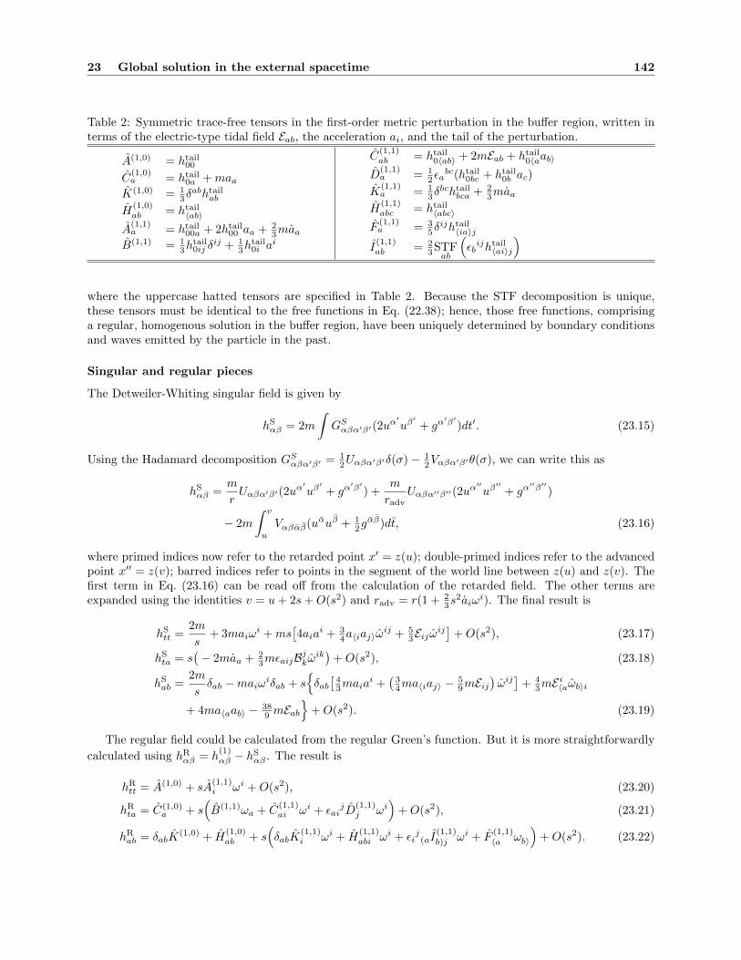
23 Global solution in the external spacetime 142
Table 2: Symmetric trace-free tensors in the first-order metric perturbation in the buffer region, written interms of the electric-type tidal field Eab, the acceleration ai, and the tail of the perturbation.
A(1,0) = htail00
C(1,0)a = htail
0a +maaK(1,0) = 1
3δabhtail
ab
H(1,0)ab = htail
〈ab〉
A(1,1)a = htail
00a + 2htail00 aa + 2
3maaB(1,1) = 1
3htail0ij δ
ij + 13h
tail0i a
i
C(1,1)ab = htail
0〈ab〉 + 2mEab + htail0〈aab〉
D(1,1)a = 1
2εabc(htail
0bc + htail0b ac)
K(1,1)a = 1
3δbchtail
bca + 23maa
H(1,1)abc = htail
〈abc〉
F(1,1)a = 3
5δijhtail〈ia〉j
I(1,1)ab = 2
3STFab
(εbijhtail〈ai〉j
)
where the uppercase hatted tensors are specified in Table 2. Because the STF decomposition is unique,these tensors must be identical to the free functions in Eq. (22.38); hence, those free functions, comprisinga regular, homogenous solution in the buffer region, have been uniquely determined by boundary conditionsand waves emitted by the particle in the past.
Singular and regular pieces
The Detweiler-Whiting singular field is given by
hSαβ = 2m
∫GSαβα′β′(2u
α′uβ′+ gα
′β′)dt′. (23.15)
Using the Hadamard decomposition GSαβα′β′ = 12Uαβα′β′δ(σ)− 1
2Vαβα′β′θ(σ), we can write this as
hSαβ =
m
rUαβα′β′(2u
α′uβ′+ gα
′β′) +m
radvUαβα′′β′′(2u
α′′uβ′′
+ gα′′β′′)
− 2m
∫ v
u
Vαβαβ(uαuβ + 12gαβ)dt, (23.16)
where primed indices now refer to the retarded point x′ = z(u); double-primed indices refer to the advancedpoint x′′ = z(v); barred indices refer to points in the segment of the world line between z(u) and z(v). Thefirst term in Eq. (23.16) can be read off from the calculation of the retarded field. The other terms areexpanded using the identities v = u+ 2s+O(s2) and radv = r(1 + 2
3s2aiω
i). The final result is
hStt =
2m
s+ 3maiω
i +ms[4aia
i + 34a〈iaj〉ω
ij + 53Eijωij
]+O(s2), (23.17)
hSta = s
(− 2maa + 2
3mεaijBjkω
ik)
+O(s2), (23.18)
hSab =
2m
sδab −maiωiδab + s
δab[
43maia
i +(
34ma〈iaj〉 − 5
9mEij)ωij]
+ 43mE i〈aωb〉i
+ 4ma〈aab〉 − 389 mEab
+O(s2). (23.19)
The regular field could be calculated from the regular Green’s function. But it is more straightforwardly
calculated using hRαβ = h
(1)αβ − hS
αβ . The result is
hRtt = A(1,0) + sA
(1,1)i ωi +O(s2), (23.20)
hRta = C(1,0)
a + s(B(1,1)ωa + C
(1,1)ai ωi + εai
jD(1,1)j ωi
)+O(s2), (23.21)
hRab = δabK
(1,0) + H(1,0)ab + s
(δabK
(1,1)i ωi + H
(1,1)abi ωi + εi
j(aI
(1,1)b)j ωi + F
(1,1)〈a ωb〉
)+O(s2). (23.22)
24 Concluding remarks 143
23.3 Equation of motion
With the metric perturbation fully determined, we can now express the self-force in terms of tail integrals.Reading off the components of hR
αβ from Table 2 and inserting the results into Eq. (22.84), we arrive at
aµ(1) = −1
2(gµν + uµuν)
(2htail
νλρ − htailλρν
) ∣∣∣a=0
uλuρ +1
2mRµνλρu
νSλρ. (23.23)
We have now firmly established the results of the point-particle analysis.
24 Concluding remarks
We have presented a number of derivations of the equations that determine the motion of a point scalarcharge q, a point electric charge e, and a point mass m in a specified background spacetime. In this concludingsection we summarize these derivations and their foundations. We conclude by describing the next step inthe gravitational case: obtaining an approximation scheme sufficiently accurate to extract the parameters ofan extreme-mass-ratio inspiral from an observed gravitational waveform.
Our derivations are of two types. The first is based on the notion of an exact point particle. In thisapproach, we assume that the self-force on the particle arises from a particular piece of its field, eitherthat which survives angle-averaging or the Detweiler-Whiting regular field. The second type is based onthe notion of an asymptotically small body, and abandons the fiction of a point particle. In this approach,we don’t assume anything about the body’s equation of motion, but rather derive it directly from the fieldequations. Although we have presented such a derivation only in the gravitational case, analogous ones couldbe performed in the scalar and electromagnetic cases, using conservation of energy-momentum instead of thefield equations alone. Such a calculation was performed by Gralla et al. in the restricted case of an electriccharge in a flat background [2].
Perhaps the essential result of our derivation based on an asymptotically small body is that it confirms allof the results derived using point particles: at linear order in the body’s mass, the field it creates is identicalto that of a point particle, and its equation of motion is precisely that derived from physically motivatedaxioms for a point particle. In other words, at linear order, not only can we get away with the fiction of apoint particle, but our assumptions about the physics governing its motion are also essentially correct.
24.1 The motion of a point particle
Spatial averaging
Our first means of deriving equations of motion for point particles is based on spatial averaging. In thisapproach, we assume the following axiom:
the force on the particle arises from the piece of the field that survives angle averaging.
For convenience in our review, we consider the case of a point electric charge and adopt the Detweiler-Whitingdecomposition of the Faraday tensor into singular and regular pieces, Fαβ = FR
αβ + F Sαβ . We average Fαβ
over a sphere of constant proper distance from the particle. We then evaluate the averaged field at theparticle’s position. Because the regular field is nonsingular on the world line, this yields
e〈Fµν〉uν = e〈F Sµν〉uν + eFR
µνuν ,
where
e〈F Sµν〉uν = −(δm)aµ, δm = lim
s→0
(2
3
e2
s
),
and
eFRµνu
ν = e2(gµν + uµuν
)(2
3aν +
1
3Rνλu
λ
)+ 2e2uν
∫ τ−
−∞∇[µG
+ν]λ′
(z(τ), z(τ ′)
)uλ′dτ ′.
We now postulate that the equations of motion are maµ = e〈Fµν〉uν , where m is the particle’s bare mass.With the preceding results we arrive at mobsaµ = eFR
µνuν , where mobs ≡ m+ δm is the particle’s observed
(renormalized) inertial mass.

24 Concluding remarks 144
In this approach, the fiction of a point particle manifests itself in the need for mass renormalization. Sucha requirement can be removed, even within the point-particle picture, by adopting the “comparison axiom”proposed by Quinn and Wald [7]. If we consider extended (but small) bodies, no such renormalization isrequired, and the equations of motion follow directly from the conservation of energy-momentum. However,the essential assumption about the nature of the force is valid: only the piece of the field that survivesangle-averaging exerts a force on the body.
The Detweiler-Whiting Axiom
Our second means of deriving equations of motion for point particles is based on the Detweiler-Whitingaxiom, which asserts that
the singular field exerts no force on the particle; the entire self-force arises from the action of theregular field.
This axiom, which is motivated by the symmetric nature of the singular field, and also its causal structure,gives rise to the same equations of motion as the averaging method. In this picture, the particle simplyinteracts with a free field (whose origin can be traced to the particle’s past), and the procedure of massrenormalization is sidestepped. In the scalar and electromagnetic cases, the picture of a particle interactingwith a free radiation field removes any tension between the nongeodesic motion of the charge and the principleof equivalence. In the gravitational case the Detweiler-Whiting axiom produces a generalized equivalenceprinciple (c.f. Ref. [156]): up to order ε2 errors, a point mass m moves on a geodesic of the spacetime withmetric gαβ + hR
αβ , which is nonsingular and a solution to the vacuum field equations. This is a conceptuallypowerful, and elegant, formulation of the MiSaTaQuWa equations of motion. And it remains valid for(non-spinning) small bodies.
Resolving historical ambiguities
Although they yield the correct physical description, the above axioms are by themselves insufficient, andhistorically, two problems have arisen in utilizing them: One, they led to ill-behaved equations of motion,requiring a process of order reduction; and two, in the gravitational case they led to equations of motionthat are inconsistent with the field equations, requiring the procedure of gauge-relaxation. Both of theseproblems arose because the expansions were insufficiently systematic, in the sense that they did not yieldexactly solvable perturbation equations. In the approach taken in our review, we have shown that theseproblems do not arise within the context of a systematic expansion. Although we have done so only in thecase of an extended body, where we sought a higher degree of rigor, one could do the same in the case ofpoint particles by expanding in the limit of small charge or mass (see, e.g., the treatment of a point mass inRef. [17]).
Consider the Abraham-Lorentz-Dirac equation maµ = fµext + 23e
2aµ. To be physically meaningful andmathematically well-justified, it must be thought of as an approximate equation of motion for a localizedmatter distribution with small charge e 1. But it contains terms of differing orders e0 and e2, and theacceleration itself is obviously a function of e. Hence, the equation has not been fully expanded. One mightthink that it is somehow an exact equation, despite its ill behaviour. Or one might replace it with the
order-reduced equation maµ = fµext + 2e2
3m fµext to eliminate that ill behaviour. But one can instead assume
that aµ(e), like other functions of e, possesses an expansion in powers of e, leading to the two well-behavedequations ma(0)µ = fµext and ma(1)µ = 2
3e2a(0)µ. However, the fact that such an equation can even arise
indicates that one has not begun with a systematic expansion of the governing field equations (in this case,the conservation equation and the Maxwell equations). If one began with a systematic expansion, withequations exactly solvable at each order, no such ambiguity would arise.
The same can be said of the second problem. It is well known that in general relativity, the motion ofgravitating bodies is determined by the Einstein field equations; the equations of motion cannot be separatelyimposed. And specifically, if we deal with the linearized Einstein equation δGαβ [h(1)] = 8πTαβ [γ], whereTαβ is the energy-momentum tensor of a point particle in the background spacetime, then the linearizedBianchi identity requires the point particle to move on a geodesic of the background spacetime. This seemsto contradict the MiSaTaQuWa equation and therefore the assumptions we made in deriving it. In order

24 Concluding remarks 145
to remove this inconsistency, the earliest derivations [6, 7] invoked an a posteriori gauge-relaxation: ratherthan solving a linearized Einstein equation exactly, they solved the wave equation Eαβ [h(1)] = −16πTαβ incombination with the relaxed gauge condition Lα[εh(1)] = O(ε2). The allowed errors in the gauge conditioncarry over into the linearized Bianchi identity, such that it no longer restricts the motion to be geodesic.In this approach, one is almost solving the linearized problem one set out to solve. But again, such an aposteriori corrective measure is required only if one begins without a systematic expansion. The first-ordermetric perturbation is a functional of a world line; if we allow that world line to depend on ε, then the metrichas evidently not been fully expanded in powers of ε. To resolve the problem, one needs to carefully dealwith this fact.
In the approach we have adopted here, following Ref. [17], we have resolved these problems via a self-consistent expansion in which the world line is held fixed while expanding the metric. Rather than beginningwith the linear field equation, we began by reformulating the exact equation in the form
Eαβ [h] = T effαβ , (24.1)
Lα[h] = 0. (24.2)
These equations we systematically expanded by (i) treating the metric perturbation as a functional of afixed world line, keeping the dependence on the world line fixed while expanding, and (ii) expanding theacceleration of the world line. Since we never sought a solution to the equation δGαβ [h(1)] = 8πTαβ [γ], notension arose between the equation of motion and the field equation. In addition, we dealt only with exactlysolvable perturbative equations: rather then imposing the ad hoc a posteriori gauge condition Lµ[εh(1)] =
O(ε2), our approach systematically led to the conditions L(0)µ
[h(1)
]= 0 and L
(1)µ
[h(1)
]= −L(0)
µ
[h(2)
], which
can be solved exactly. Like in the issue of order reduction, the essential step in arriving at exactly solvableequations is assuming an expansion of the particle’s acceleration.
Historically, these issues were first resolved by Gralla and Wald [16] using a different method. Ratherthan allowing an ε-dependence in the first-order perturbation, they fully expanded every function in theproblem in a power series, including the world line itself. In this approach, the world line of the body isfound to be a geodesic, but higher-order effects arise in deviation vectors measuring the drift of the particleaway from that geodesic. Such a method has the drawback of being limited to short timescales, since thedeviation vectors will eventually grow large as the body moves away from the initial reference geodesic.
24.2 The motion of a small body
Although the above results for point particles require assumptions about the form of the force, their resultshave since been derived from first principles, and the physical pictures they are based on have proven to bejustified: An asymptotically small body behaves as a point particle moving on a geodesic of the smooth partof the spacetime around it, or equivalently, it moves on a world line accelerated by the asymmetric part ofits own field.
In addition to a derivation from first principles, we also seek a useful approximation scheme. Any suchscheme must deal with the presence of multiple distinct scales. Most obviously, these are the mass and sizeof the body itself and the lengthscales of the external universe, but other scales also arise. For example, inorder to accurately represent the physics of an extreme-mass-ratio system, we must consider changes overfour scales: First, there is the large body’s mass, which is the characteristic lengthscale of the externaluniverse. For convenience, since all lengths are measured relative to this one, we rescale them such thatthis global lengthscale is ∼ 1. Second, there is the small body’s mass ∼ ε, which is the scale over whichthe gravitational field changes near the body; since the body is compact, this is also the scale of its linearsize. Third, there is the radiation-reaction time ∼ 1/ε; this is the time over which the small effects of theself-force accumulate to produce significant changes, specifically the time required for quantities such asthe small body’s energy and angular momentum to accumulate order 1 changes. Fourth, there is the largedistance to the wave zone. We will not discuss this last scale here, but dealing with it analytically wouldlikely require matching a wave solution at null infinity to an expansion formally expected to be valid in aregion of size ∼ 1/ε.

24 Concluding remarks 146
Self-consistent and matched asymptotic expansions
In this review, we have focused on a self-consistent approximation scheme first presented in Refs. [17,18,129].It deals with the small size of the body using two expansions. Near the body, to capture changes on theshort distances ∼ ε, we adopt an inner expansion in which the body remains of constant size while all otherdistances approach infinity. Outside of this small neibourhood around the body, we adopt an outer expansionin which the body shrinks to zero mass and size about an ε-dependent world line that accurately reflectsits long-term motion. The world line γ is defined in the background spacetime of the outer expansion. Itsacceleration is found by solving the Einstein equation in a buffer region surrounding the body, where bothexpansions are valid; in this region, both expansions must agree, and we can use the multipole moments ofthe inner expansion to determine the outer one. In particular, we define γ to be the body’s world line ifand only if the body’s mass dipole moment vanishes when calculated in coordinates centered on it. As inthe point-particle calculation, the essential step in arriving at exactly solvable equations and a well-behavedequation of motion is an assumed expansion of the acceleration on the world line.
In order to construct a global solution in the outer expansion, we first recast the Einstein equation ina form that can be expanded and solved for an arbitrary world line. As in the point-particle case, weaccomplish this by adopting the Lorenz gauge for the total metric perturbation. We can then write formalsolutions to the perturbation equations at each order as integrals over a small tube surrounding the body(plus an initial data surface). By embedding the tube in the buffer region, we can use the data from thebuffer-region expansion to determine the global solution. At first order, we find that the metric perturbationis precisely that of a point particle moving on the world line γ. While the choice of gauge is not essentialin finding an expression for the force in terms of the field in the buffer-region expansion, it is essential inour method of determining the global field. Without making use of the relaxed Einstein equations, no clearmethod of globally solving the Einstein equation presents itself, and no simple split between the perturbationand the equation of motion arises.
Because this expansion self-consistently incorporates the corrections to the body’s motion, it promisesto be accurate on long timescales. Specifically, when combined with the first-order metric perturbation, thefirst-order equation of motion defines a solution to the Einstein equation that we expect to be accurate up toorder ε2 errors over times t . 1/ε. When combined with the second-order perturbation, it defines a solutionwe expect to be accurate up to order ε3 errors on the shorter timescale ∼ 1.
This approach closely mirrors the extremely successful methods of post-Newtonian theory [156]. Inparticular, both schemes recast the Einstein equation in a relaxed form before expanding it. Also, our use ofan inner limit near the body is analogous to the “strong-field point particle limit” exploited by Futamase andhis collaborators [156]. And our calculation of the equation of motion is somewhat similar to the methodsused by Futamase and others [156,174], in that it utilizes a multipole expansion of the body’s metric in thebuffer region.
Alternative methods
Various other approaches have been taken to deal with the multiple scales in the problem. In particular,even the earliest paper on the gravitational self-force [6] made use of inner and outer limits, which were alsoused in different forms in later derivations [15, 33, 183]. However, those early derivations are problematic.Specifically, they never adequately define the world line for which they derive equations of motion.
In the method of matched asymptotic expansions used in Refs. [6, 15,33], the first-order perturbation inthe outer expansion is assumed to be that of a point particle, with an attendant world line, and the innerexpansion is assumed to be that of a perturbed black hole; by matching the two expansions in the bufferregion, the acceleration of the world line is determined. Since the forms of the inner and outer expansions arealready restricted, this approach’s conclusions have somewhat limited strength, but it has more fundamentalproblems as well. The matching procedure begins by expanding the outer expansion in powers of distance s(or r) from the world line, and the inner expansion for large spacial distances R ε. But the two expansionsbegin in different coordinate systems with an unknown relationship between them. In particular, there isno given relationship between the world line and the “position” of the black hole. The two expansionsare matched by finding a coordinate transformation that makes them agree in the buffer region. However,because there is no predetermined relationship between the expansions, this transformation is not in factunique, and it does not yield a unique equation of motion. One can increase the strength of the matching
24 Concluding remarks 147
condition in order to arrive at unique results, but that further weakens the strength of the conclusions. Referto Ref. [18] for a discussion of these issues.
Rather than finding the equation of motion from the field equations, as in the above calculations, Fuku-moto et al. [183] found the equation of motion by defining the body’s linear momentum as an integral overthe body’s interior and then taking the derivative of that momentum. But they then required an assumedrelationship between the momentum and the four-velocity of a representative world line in the body’s inte-rior. Hence, the problem is again an inadequate defintion of the body’s motion. Because it involves integralsover the body’s interior, and takes the world line to lie therein, this approach is also limited to materialbodies; it does not apply to black holes.
The first reliable derivation of the first-order equation of motion for an asymptotically small body wasperformed by Gralla and Wald [16], who used a method of the same nature as the one presented here,deriving equations of motion by solving the field equations in the buffer region. As we have seen, however,their derivation is based on an expansion of the world line in powers of ε instead of a self-consistent treatmentthat keeps it fixed.
Using very different methods, Harte has also provided reliable derivations of equations of motion forextended bodies interacting with their own scalar and electromagnetic fields in fixed background space-times [157, 158, 181]. His approach is based on generalized definitions of momenta, the evolution of whichis equivalent to energy-momentum conservation. The momenta are defined in terms of generalized Killingfields ξα, the essential property of which is that they satisfy £ξgαβ |γ = ∇γ£ξgαβ |γ = 0 — that is, they satisfyKilling’s equation on the body’s world line and approximately satisfy it “nearby.” Here the world line canbe defined in multiple ways using, for example, center-of-mass conditions. This approach is nonperturbative,with no expansion in the limit of small mass and size (though it does require an upper limit on the body’ssize and a lower limit on its compactness). It has the advantage of very naturally deriving a generalizationof the Detweiler-Whiting axiom: The field of an extended body can be split into (i) a solution to the vacuumfield equations which exerts a direct self-force, and (ii) a solution to the equations sourced by the body,which shifts the body’s multipole moments. This approach has not yet been applied to gravity, but such anapplication should be relatively straightforward. However, as with the approach of Fukumoto et al. [183],this one does not apply to black holes.
Other methods have also been developed (or suggested) to accomplish the same goals as the self-consistentexpansion. Most prominent among these is the two-timescale expansion suggested by Hinderer and Flanagan[121]. As discussed in Sec. 2, their method splits the orbital evolution into slow and fast dynamics byintroducing slow and fast time variables. In the terminology of Sec. 22, this method constructs a generalexpansion by smoothly transitioning between regular expansions constructed at each value of the slow timevariable, with the transition determined by the evolution with respect to the slow time. On the scaleof the fast time, the world line is a geodesic; but when the slow time is allowed to vary, the world linetransitions between geodesics to form the true, accelerated world line. This results in a global, uniform-in-time approximation. One should note that simply patching together a sequence of regular expansions,by shifting to a new geodesic every so often using the deviation vector, would not accomplish this: Sucha procedure would accumulate a secular error in both the metric perturbation and the force, because theperturbation would be sourced by a world line secularly deviating from the position of the body, and theforce would be calculated from this erroneous perturbation. The error would be proportional to the numberof “shifts” multiplied by a nonlinear factor depending on the time between them. And this error would,formally at least, be of the same magnitude as the solution itself.
The fundamental difference between the self-consistent expansion and the two-timescale expansion is thefollowing: In the two-timescale method, the Einstein equation, coupled to the equation of motion of the smallbody, is reduced to a dynamical system that can be evolved in time. The true world line of the body thenemerges from the evolution of this system. In the method presented here, we have instead sought global,formal solutions to the Einstein equation, written in terms of global integrals; to accomplish this, we havetreated the world line of the body as a fixed structure in the external spacetime. However, the two methodsshould agree. Note, though, that the two-timescale expansion is limited to orbits in Kerr, and it requiresevolution equations for the slow evolution of the large black hole’s mass and spin parameters, which havenot yet been derived. Since the changes in mass and spin remain small on a radiation-reaction timescale, in
the self-consistent expansion presented here they are automatically incorporated into the perturbations h(n)αβ .
It is possible that this incorporation leads to errors on long timescales, in which case a different approach,
24 Concluding remarks 148
naturally allowing slow changes in the background, would be more advantageous.
24.3 Beyond first order
The primary experimental motivation for researching the self-force is to produce waveform templates forLISA. In order to extract the parameters of an extreme-mass-ratio binary from a waveform, we require awaveform that is accurate up to errors of order ε after a radiation-reaction time ∼ 1/ε. If we use the first-order equation of motion, we will be neglecting an acceleration ∼ ε2, which will lead to secular errors oforder unity after a time ∼ 1/ε. Thus, the second-order self-force is required in order to obtain a sufficientlyaccurate waveform template. In order to achieve the correct waveform, we must also obtain the second-order part of the metric perturbation; this can be easily done, at least formally, using the global integralrepresentations outside a world tube. However, a practical numerical calculation may prove difficult, sinceone would not wish to excise the small tube from one’s numerical domain, and the second-order perturbationwould diverge too rapidly on the world line to be treated straightforwardly.
A formal expression for the second-order force has already been derived by Rosenthal [184,185]. However,he expresses the second-order force in a very particular gauge in which the first-order self-force vanishes. Thisis sensible on short timescales, but not on long timescales, since it forces secular changes into the first-orderperturbation, presumably leading to the first-order perturbation becoming large with time. Furthermore,it is not a convenient gauge, since it does not provide what we wish it to: a correction to the nonzeroleading-order force in the Lorenz gauge.
Thus, we wish to obtain an alternative to Rosenthal’s derivation. Based on the methods reviewed inthis article, there is a clear route to deriving the second-order force. One would construct a buffer-regionexpansion accurate up to order ε3. Since one would require the order ε2s terms in this expansion, in order todetermine the acceleration, one would need to increase the order of the expansion in r as well. Specifically,one would need terms up to orders ε0s3, εs2, ε2s, and ε3s0. In such a calculation, one would expect thefollowing terms to appear: the body’s quadrupole moment Qab, corrections δMi and δSi to its mass and spindipoles, and a second-order correction δ2m to its mass. Although some ambiguity may arise in defining theworld line of the body at this order, a reasonable definition appears to be to guarantee that δMi vanishes.However, at this order one may require some model of the body’s internal dynamics, since the equationof motion will involve the body’s quadrupole moment, for which the Einstein equation is not expected toyield an evolution equation. But if one seeks only the second-order self-force, one could simply neglect thequadrupole by assuming that the body is spherically symmetric in isolation. In any case, the force dueto the body’s quadrupole moment is already known from various other methods: see, e.g., the work ofDixon [159–161]; more recent methods can be found in Ref. [186] and references therein.
Because such a calculation could be egregiously lengthy, one may consider simpler methods, perhapsrequiring stronger assumptions. For example, one could straightforwardly implement the method of matchedasymptotic expansions with the matching conditions discussed in Ref. [18], in which one makes strongassumptions about the relationship between the inner and outer expansions. The effective field theorymethod used by Galley and Hu [163] offers another possible route.
Alternatively, one could calculate only part of the second-order force. Specifically, as described in Sec. 2.5,Hinderer and Flanagan [121,130] have shown that one requires in fact only the averaged dissipative part ofthe second-order force. This piece of the force can be calculated within an adiabatic approximation, in whichthe rates of change of orbital parameters are calculated from the radiative Green’s function, asymptotic waveamplitudes, and information about the orbit that sources them. Hence, we might be able to forgo a completecalculation of the second-order force, and use instead the complete first-order force in conjunction with anadiabatic approximation for the second-order force.
The self-force, however, is of interest beyond its relevance to LISA. The full second-order force would beuseful for more general purposes, such as more accurate comparisons to post-Newtonian theory, and analysisof other systems, such as intermediate mass ratio binaries. Perhaps most importantly, it is of fundamentalimportance in our understanding of the motion of small bodies. For these reasons, proceeding to secondorder in a systematic expansion, and thereby obtaining second-order expressions for the force on a smallbody, remains an immediate goal.

A Second-order expansions of the Ricci tensor 149
Appendices
A Second-order expansions of the Ricci tensor
We present here various expansions used in solving the second-order Einstein equation in Sec. 22.4. Werequire an expansion of the second-order Ricci tensor δ2Rαβ , defined by
δ2Rαβ [h] = − 12γ
µν;ν
(2hµ(α;β) − hαβ;µ
)+ 1
4hµν
;αhµν;β + 12h
µβ
;ν (hµα;ν − hνα;µ)
− 12h
µν(2hµ(α;β)ν − hαβ;µν − hµν;αβ
), (A.1)
where γµν is the trace-reversed metric perturbation, and an expansion of a certain piece of Eµν [h(2)]. Specif-
ically, we require an expansion of δ2R(0)αβ [h(1)] in powers of the Fermi radial coordinate s, where for a function
f , δ2R(0)αβ [f ] consists of δ2Rαβ [f ] with the acceleration aµ set to zero. We write
δ2R(0)αβ [h(1)] =
1
s4δ2R
(0,−4)αβ
[h(1)
]+
1
s3δ2R
(0,−3)αβ
[h(1)
]+
1
s2δ2R
(0,−2)αβ
[h(1)
]+O(1/s), (A.2)
where the second superscript index in parentheses denotes the power of s. Making use of the expansion of
h(1)αβ , obtained by setting the acceleration to zero in the results for h
(1)αβ found in Sec. 22.3, one finds
δ2R(2,−4)αβ
[h(1)
]= 2m2
(7ωab + 4
3δab)xaαx
bβ − 2m2tαtβ , (A.3)
and
δ2R(2,−3)tt
[h(1)
]= 3mH
(1,0)ij ωij , (A.4)
δ2R(2,−3)ta
[h(1)
]= 3mC
(1,0)i ωia, (A.5)
δ2R(2,−3)ab
[h(1)
]= 3m
(A(1,0) + K(1,0)
)ωab − 6mH
(1,0)i〈a ωib〉 +mδabH
(1,0)ij ωij , (A.6)
and
δ2R(2,−2)tt
[h(1)
]= − 20
3 m2Eijωij + 3mH
(1,1)ijk ωijk + 7
5mA(1,1)i ωi + 3
5mK(1,1)i ωi
− 45m∂tC
(1,0)i ωi, (A.7)
δ2R(2,−2)ta
[h(1)
]= −m∂tK(1,0)ωa + 3mC
(1,1)ij ωa
ij +m(
65 C
(1,1)ai − ∂tH(1,0)
ai
)ωi
+ 2mεaijD
(1,1)i ωj + 4
3m2εaikBkj ωij , (A.8)
δ2R(2,−2)ab
[h(1)
]= δabm
(1615∂tC
(1,0)i − 13
15 A(1,1)i − 9
5K(1,1)i
)ωi
+ δab
(− 50
9 m2Eijωij +mH
(1,1)ijk ωijk
)− 14
3 m2Eijωabij
+m(
3310 A
(1,1)i + 27
10K(1,1)i − 3
5∂tC(1,0)i
)ωab
i
+m(
2825 A
(1,1)〈a − 18
25K(1,1)〈a − 46
25∂tC(1,0)〈a
)ωb〉
− 83m
2Ei〈aωb〉i − 6mH(1,1)ij〈a ωb〉
ij + 3mεij(aωb)jk I
(1,1)ik
+ 245m
2Eab − 25mH
(1,1)abi ωi + 8
5mεij(aI
(1,1)b)i ωj . (A.9)
Next, we require an analogous expansion of E(0)αβ
[1r2h
(2,−2) + 1rh
(2,−1)], where E
(0)αβ [f ] is defined for any
f by setting the acceleration to zero in Eαβ [f ]. The coefficients of the 1/r4 and 1/r3 terms in this expansion
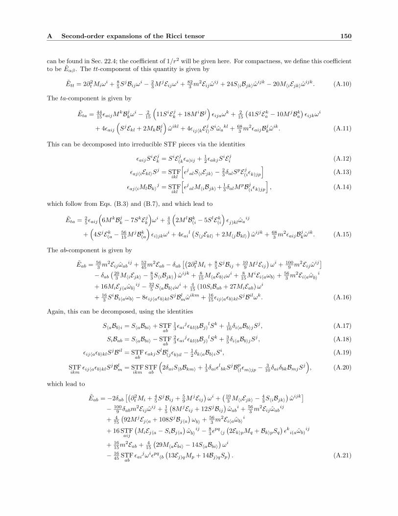
A Second-order expansions of the Ricci tensor 150
can be found in Sec. 22.4; the coefficient of 1/r2 will be given here. For compactness, we define this coefficientto be Eαβ . The tt-component of this quantity is given by
Ett = 2∂2tMiω
i + 85S
jBijωi − 23M
jEijωi + 823 m
2Eijωij + 24S〈iBjk〉ωijk − 20M〈iEjk〉ωijk. (A.10)
The ta-component is given by
Eta = 4415εaijM
kBjkωi − 215
(11SiEjk + 18M iBj
)εijaω
k + 215
(41SjEka − 10M jBka
)εijkω
i
+ 4εaij
(SjEkl + 2MkBjl
)ωikl + 4εij〈kEjl〉Siωakl + 68
3 m2εaijBjkωik. (A.11)
This can be decomposed into irreducible STF pieces via the identities
εaijSiEjk = SiEj(kεa)ij + 1
2εakjSiEji (A.12)
εaj〈iEkl〉Sj = STFikl
[εjalS〈iEjk〉 − 2
3δalSpEj(iεk)jp
](A.13)
εaj〈iMlBk〉j = STFikl
[εjalM〈iBjk〉+ 1
3δalMpBj(iεk)jp
], (A.14)
which follow from Eqs. (B.3) and (B.7), and which lead to
Eta = 25εaij
(6MkBjk − 7SkEjk
)ωi + 4
3
(2M lBk(i − 5SlEk(i
)εj)klωa
ij
+(
4SjEk(a − 5615M
jBk(a)εi)jkω
i + 4εail(S〈jEkl〉 + 2M〈jBkl〉
)ωijk + 68
3 m2εaijBjkωik. (A.15)
The ab-component is given by
Eab = 563 m
2Eijωabij + 5245m
2Eab − δab[(
2∂2tMi + 8
5SjBij + 10
9 MjEij
)ωi + 100
9 m2Eijωij]
− δab(
203 M〈iEjk〉 − 8
3S〈iBjk〉)ωijk + 8
15M〈aEb〉iωi + 815M
iEi〈aωb〉 + 563 m
2Ei〈aωb〉i
+ 16MiEj〈aωb〉ij − 325 S〈aBb〉iωi + 4
15 (10SiBab + 27MiEab)ωi
+ 163 S
iBi〈aωb〉 − 8εij〈aεb〉klSjBlmωikm + 16
15εij〈aεb〉klSjBilωk. (A.16)
Again, this can be decomposed, using the identities
S〈aBb〉i = S〈aBbi〉 + STFab
13εai
jεkl(bBj)lSk + 110δi〈aBb〉jSj , (A.17)
SiBab = S〈aBbi〉 − STFab
23εai
jεkl(bBj)lSk + 35δi〈aBb〉jSj , (A.18)
εij〈aεb〉klSjBil = STF
abεakjS
lBi(jεb)il − 12δk〈aBb〉iSi, (A.19)
STFikm
εij〈aεb〉klSjBlm = STF
ikmSTFab
(2δaiS〈bBkm〉 + 1
3δaiεlbkS
jBp(lεm)jp − 310δaiδbkBmjSj
), (A.20)
which lead to
Eab = −2δab[(∂2tMi + 4
5SjBij + 5
9MjEij
)ωi +
(103 M〈iEjk〉 − 4
3S〈iBjk〉)ωijk
]− 100
9 δabm2Eijωij + 1
5
(8M jEij + 12SjBij
)ωab
i + 563 m
2Eijωabij
+ 475
(92M jEj〈a + 108SjBj〈a
)ωb〉 + 56
3 m2Ei〈aωb〉i
+ 16 STFaij
(MiEj〈a − SiBj〈a
)ωb〉
ij − 83εpq〈j(2Ek〉pMq + Bk〉pSq
)εki(aωb)
ij
+ 1615m
2Eab + 415
(29M〈aEbi〉 − 14S〈aBbi〉
)ωi
− 1645 STF
abεai
jωiεpq(b
(13Ej)qMp + 14Bj)qSp
). (A.21)

B STF multipole decompositions 151
B STF multipole decompositions
All formulas in this Appendix are either taken directly from Refs. [187] and [180] or are easily derivable fromformulas therein.
Any Cartesian tensor field depending on two angles θA spanning a sphere can be expanded in a uniquedecomposition in symmetric trace-free tensors. Such a decomposition is equivalent to a decomposition intensorial harmonics, but it is sometimes more convenient. It begins with the fact that the angular dependenceof a Cartesian tensor TS(θA) can be expanded in a series of the form
TS(θA) =∑`≥0
TS〈L〉ωL, (B.1)
where S and L denote multi-indices S = i1 . . . is and L = j1 . . . j`, angular brackets denote an STF combina-tion of indices, ωa is a Cartesian unit vector, ωL := ωj1 . . . ωj` , and ωL := ω〈L〉. This is entirely equivalentto an expansion in spherical harmonics. Each coefficient TS〈L〉 can be found from the formula
TS〈L〉 =(2`+ 1)!!
4π`!
∫TS(θA)ωLdΩ, (B.2)
where the double factorial is defined by x!! = x(x− 2) · · · 1. These coefficients can then be decomposed intoirreducible STF tensors. For example, for s = 1, we have
Ta〈L〉 = T(+1)aL + εja〈i` T
(0)L−1〉j + δa〈i` T
(−1)L−1〉, (B.3)
where the T (n)’s are STF tensors given by
T(+1)L+1 := T〈L+1〉, (B.4)
T(0)L :=
`
`+ 1Tpq〈L−1εi`〉
pq, (B.5)
T(−1)L−1 :=
2`− 1
2`+ 1T jjL−1. (B.6)
Similarly, for a symmetric tensor TS with s = 2, we have
Tab〈L〉 = STFL
STFab
(εpai` T
(+1)bpL−1 + δai` T
(0)bL−1 + δai`ε
pbi`−1
T(−1)pL−2 + δai`δbi`−1
T(−2)L−2
)+ T
(+2)abL + δabKL, (B.7)
where
T(+2)L+2 := T〈L+2〉, (B.8)
T(+1)L+1 :=
2`
`+ 2STFL+1
(T〈pi`〉qL−1εi`+1
pq), (B.9)
T(0)L :=
6`(2`− 1)
(`+ 1)(2`+ 3)STFL
(T〈ji`〉jL−1), (B.10)
T(−1)L−1 :=
2(`− 1)(2`− 1)
(`+ 1)(2`+ 1)STFL−1
(T〈jp〉qjL−2εi`−1
pq), (B.11)
T(−2)L−2 :=
2`− 3
2`+ 1T〈jk〉
jkL−2 (B.12)
KL := 13T
jjL. (B.13)
These decompositions are equivalent to the formulas for addition of angular momenta, J = S + L, whichresults in terms with angular momentum ` − s ≤ j ≤ ` + s; the superscript labels (±n) in these formulasindicate by how much each term’s angular momentum differs from `.
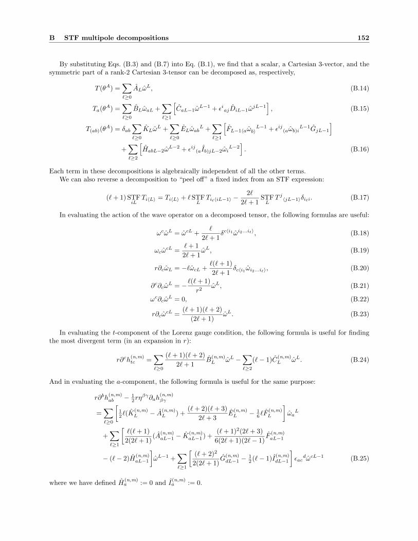
B STF multipole decompositions 152
By substituting Eqs. (B.3) and (B.7) into Eq. (B.1), we find that a scalar, a Cartesian 3-vector, and thesymmetric part of a rank-2 Cartesian 3-tensor can be decomposed as, respectively,
T (θA) =∑`≥0
ALωL, (B.14)
Ta(θA) =∑`≥0
BLωaL +∑`≥1
[CaL−1ω
L−1 + εiajDiL−1ωjL−1
], (B.15)
T(ab)(θA) = δab
∑`≥0
KLωL +
∑`≥0
ELωabL +
∑`≥1
[FL−1〈aωb〉
L−1 + εij(aωb)iL−1GjL−1
]+∑`≥2
[HabL−2ω
L−2 + εij(aIb)jL−2ωiL−2
]. (B.16)
Each term in these decompositions is algebraically independent of all the other terms.We can also reverse a decomposition to “peel off” a fixed index from an STF expression:
(`+ 1) STFiL
Ti〈L〉 = Ti〈L〉 + ` STFL
Ti`〈iL−1〉 −2`
2`+ 1STFL
T j〈jL−1〉δi`i. (B.17)
In evaluating the action of the wave operator on a decomposed tensor, the following formulas are useful:
ωcωL = ωcL +`
2`+ 1δc〈i1 ωi2...i`〉, (B.18)
ωcωcL =
`+ 1
2`+ 1ωL, (B.19)
r∂cωL = −`ωcL +`(`+ 1)
2`+ 1δc〈i1 ωi2...i`〉, (B.20)
∂c∂cωL = −`(`+ 1)
r2ωL, (B.21)
ωc∂cωL = 0, (B.22)
r∂cωcL =
(`+ 1)(`+ 2)
(2`+ 1)ωL. (B.23)
In evaluating the t-component of the Lorenz gauge condition, the following formula is useful for findingthe most divergent term (in an expansion in r):
r∂ch(n,m)tc =
∑`≥0
(`+ 1)(`+ 2)
2`+ 1B
(n,m)L ωL −
∑`≥2
(`− 1)C(n,m)L ωL. (B.24)
And in evaluating the a-component, the following formula is useful for the same purpose:
r∂bh(n,m)ab − 1
2rηβγ∂ah
(n,m)βγ
=∑`≥0
[12`(K
(n,m)L − A(n,m)
L ) +(`+ 2)(`+ 3)
2`+ 3E
(n,m)L − 1
6`F(n,m)L
]ωa
L
+∑`≥1
[`(`+ 1)
2(2`+ 1)(A
(n,m)aL−1 − K
(n,m)aL−1 ) +
(`+ 1)2(2`+ 3)
6(2`+ 1)(2`− 1)F
(n,m)aL−1
− (`− 2)H(n,m)aL−1
]ωL−1 +
∑`≥1
[(`+ 2)2
2(2`+ 1)G
(n,m)dL−1 − 1
2 (`− 1)I(n,m)dL−1
]εac
dωcL−1 (B.25)
where we have defined H(n,m)a := 0 and I
(n,m)a := 0.

B STF multipole decompositions 153
The unit vector ωi satisfies the following integral identities:∫ωLdΩ = 0 if ` > 0, (B.26)∫ωLdΩ = 0 if ` is odd, (B.27)∫ωLdΩ = 4π
δi1i2 . . . δi`−1i`
(`+ 1)!!if ` is even, (B.28)
where the curly braces indicate the smallest set of permutations of indices that make the result symmetric.For example, δabωc = δabωc + δbcωa + δcaωb.
REFERENCES 154
References
[1] P. Dirac, Classical theory of radiating electrons, Proc. R. Soc. London, Ser. A 167, 148 (1938).
[2] S. E. Gralla, A. I. Harte, and R. M. Wald, A rigorous derivation of electromagnetic self-force, Phys.Rev. D80, 024031 (2009).
[3] F. Rohrlich, Classical charged particles (Addison-Wesley, Redwood City, CA, U.S.A., 1990).
[4] B. DeWitt and R. Brehme, Radiation Damping in a Gravitational Field , Ann. Phys. (N.Y.) 9, 220(1960).
[5] J. Hobbs, A vierbein formalism for radiation damping , Ann. Phys. (N.Y.) 47, 141 (1968).
[6] Y. Mino, M. Sasaki, and T. Tanaka, Gravitational radiation reaction to a particle motion, Phys. Rev.D 55, 3457 (1997).
[7] T. Quinn and R. Wald, Axiomatic approach to electromagnetic and gravitational radiation reaction ofparticles in curved spacetime, Phys. Rev. D 56, 3381 (1997).
[8] T. Quinn, Axiomatic approach to radiation reaction of scalar point particles in curved spacetime, Phys.Rev. D 62, 064029 (2000).
[9] J. Jackson, Classical Electrodynamics, Third Edition (Wiley, New York, NY, U.S.A., 1999).
[10] C. Teitelboim, D. Villarroel, and C. van Weert, Classical electrodynamics of retarded fields and pointparticles, Riv. Nuovo Cimento 3, 9 (1980).
[11] L. D. Landau and E. M. Lifshitz, The classical theory of fields, fourth edition (Butterworth-Heinemann,Oxford, England, 2000).
[12] E. Flanagan and R. Wald, Does back reaction enforce the averaged null energy condition in semiclassicalgravity? , Phys. Rev. D 54, 6233 (1996).
[13] S. Detweiler and B. Whiting, Self-force via a Green’s function decomposition, Phys. Rev. D 67, 024025(2003).
[14] J. Synge, Relativity: The general theory (North-Holland, Amsterdam, The Netherlands, 1960).
[15] E. Poisson, Retarded coordinates based at a world line and the motion of a small black hole in anexternal universe, Phys. Rev. D 69, 084007 (2004).
[16] S. E. Gralla and R. M. Wald, A rigorous derivation of gravitational self-force, Class. Quant. Grav. 25,205009 (2008).
[17] A. Pound, Self-consistent gravitational self-force, Phys. Rev. D 81, 024023 (2010).
[18] A. Pound, Singular perturbation techniques in the gravitational self-force problem, Phys. Rev. D 81,124009 (2010).
[19] L. Barack and A. Ori, Gravitational self-force and gauge transformations, Phys. Rev. D 64, 124003(2001).
[20] LISA Home Page: http://lisa.jpl.nasa.gov.
[21] A. Smith and C. Will, Force on a static charge outside a Schwarzschild black hole, Phys. Rev. D 22,1276 (1980).
[22] A. I. Zel’nikov and V. P. Frolov, Influence of gravitation on the self-energy of charged particles, Sov.Phys. JETP 55, 919 (1982).
[23] E. Copson, On electrostatics in a gravitational field , Proc. R. Soc. London, Ser. A 116, 720 (1928).

REFERENCES 155
[24] B. Linet, Electrostatics and magnetostatics in Schwarzschild metric, J. Phys. A 9, 1081 (1976).
[25] B. Leaute and B. Linet, Electrostatics in a Reissner-Nordstrom space-time, Phys. Lett. A 58, 5 (1976).
[26] A. Wiseman, Self-force on a static scalar test charge outside a Schwarzschild black hole, Phys. Rev. D61, 084014 (2000).
[27] C. Misner, K. Thorne, and J. Wheeler, Gravitation (Freeman, San Francisco, CA, U.S.A., 1973).
[28] F. Manasse and C. Misner, Fermi normal coordinates and some basic concepts in differential geometry ,J. Math. Phys. 4, 735 (1963).
[29] J. Hadamard, Lectures on Cauchy’s problem in linear partial differential equations (Yale UniversityPress, New Haven, CT, U.S.A., 1923).
[30] F. Friedlander, The wave equation on a curved spacetime (Cambridge University Press, Cambridge,U.K., 1975).
[31] L. Barack, Gravitational self force in extreme mass-ratio inspirals, Class. Quantum Grav. 26, 213001(2009).
[32] C. Lousto (editor), Gravitational radiation from binary black holes: advances in the perturbative ap-proach, volume 22 (Class. Quantum Grav., 2005).
[33] S. Detweiler, Perspective on gravitational self-force analyses, Class. Quantum Grav. 22, 681 (2005).
[34] B. Whiting, Identifying the singular field for self-force evaluation, Class. Quantum Grav. 22, S661(2005).
[35] C. Morette-DeWitt and B. DeWitt, Falling charges, Physics (Long Island City, N.Y.) 1, 3 (1964).
[36] M. Pfenning and E. Poisson, Scalar, electromagnetic, and gravitational self-forces in weakly curvedspacetimes, Phys. Rev. D 65, 084001 (2002).
[37] L. Barack and A. Ori, Mode sum regularization approach for the self-force in black hole spacetime,Phys. Rev. D 61, 061502 (2000).
[38] L. Barack, Self-force on a scalar particle in spherically symmetric spacetime via mode-sum regulariza-tion: Radial trajectories, Phys. Rev. D 62, 084027 (2000).
[39] L. Barack, Y. Mino, H. Nakano, A. Ori, and M. Sasaki, Calculating the gravitational self-Force inSchwarzschild spacetime, Phys. Rev. Lett. 88, 091101 (2002).
[40] L. Barack, Gravitational self-force by mode sum regularization, Phys. Rev. D 64, 084021 (2001).
[41] L. Barack and A. Ori, Regularization parameters for the self-force in Schwarzschild spacetime: Scalarcase, Phys. Rev. D 66, 084022 (2002).
[42] L. Barack and A. Ori, Regularization parameters for the self-force in Schwarzschild spacetime. II.Gravitational and electromagnetic cases, Phys. Rev. D 67, 024029 (2003).
[43] L. Barack and A. Ori, Gravitational self-force on a particle orbiting a Kerr black hole, Phys. Rev. Lett.90, 111101 (2003).
[44] Y. Mino, H. Nakano, and M. Sasaki, Covariant self-force regularization of a particle orbiting aSchwarzschild black hole – Mode decomposition regularization, Prog. Theor. Phys. 108, 1039 (2003).
[45] C. Lousto, Pragmatic approach to gravitational radiation reaction in binary black holes, Phys. Rev.Lett. 84, 5251 (2000).
[46] S. Detweiler, E. Messaritaki, and B. Whiting, Self-force of a scalar field for circular orbits about aSchwarzschild black hole, Phys. Rev. D 67, 104016 (2003).
REFERENCES 156
[47] L. Burko, A. Harte, and E. Poisson, Mass loss by a scalar charge in an expanding universe, Phys. Rev.D 65, 124006 (2002).
[48] R. Haas and E. Poisson, Mass change and motion of a scalar charge in cosmological spacetimes, Class.Quantum Grav. 22, S739 (2005).
[49] K. Shankar and B. Whiting, Self-force of a static electric charge near a Schwarzschild star , Phys. Rev.D 76, 124027 (2007).
[50] R. Haas and E. Poisson, Mode-sum regularization of the scalar self-force: Formulation in terms of atetrad decomposition of the singular field , Phys. Rev. D 74, 004009 (2006).
[51] L. Burko, Self-force on static charges in Schwarzschild spacetime, Class. Quantum Grav. 17, 227(2000).
[52] L. Burko, Y. Liu, and Y. Soen, Self-force on charges in the spacetime of spherical shells, Phys. Rev. D63, 024015 (2001).
[53] L. Barack and L. Burko, Radiation-reaction force on a particle plunging into a black hole, Phys. Rev.D 62, 084040 (2000).
[54] L. Burko, Self-force on a particle in orbit around a black hole, Phys. Rev. Lett. 84, 4529 (2000).
[55] P. Canizares and C. Sopuerta, Efficient pseudospectral method for the computation of the self-force ona charged particle: Circular geodesics around a Schwarzschild black hole, Phys. Rev. D 79, 084020(2009).
[56] R. Haas, Scalar self-force on eccentric geodesics in Schwarzschild spacetime: a time-domain computa-tion, Phys. Rev. D 75, 124011 (2007).
[57] R. Haas, Self-force on point particles in orbit around a schwarzschild black hole, Ph.D. thesis, Universityof Guelph (2008).
[58] L. Barack and N. Sago, Gravitational self-force on a particle in circular orbit around a Schwarzschildblack hole, Phys. Rev. D 75, 064021 (2007).
[59] S. Akcay, Fast frequency-domain algorithm for gravitational self-force: Circular orbits in Schwarzschildspacetime, Phys. Rev. D 83, 124026 (2011).
[60] L. Barack and N. Sago, Gravitational self-force correction to the innermost stable circular orbit of aSchwarzschild black hole, Phys. Rev. Lett. 102, 191101 (2009).
[61] S. Detweiler, Consequence of the gravitational self-force for circular orbits of the Schwarzschild geom-etry , Phys. Rev. D 77, 124026 (2008).
[62] N. Sago, L. Barack, and S. Detweiler, Two approaches for the gravitational self force in black holespacetime: Comparison of numerical results, Phys. Rev. D 78, 124024 (2008).
[63] L. Barack, T. Damour, and N. Sago, Precession effect of the gravitational self-force in a Schwarzschildspacetime and the effective one-body formalism, Phys. Rev. D 82, 084036 (2010).
[64] L. Blanchet, S. Detweiler, A. Le Tiec, and B. Whiting, Post-Newtonian and numerical calculations ofthe gravitational self-force for circular orbits in the Schwarzschild geometry , Phys. Rev. D 81, 064004(2010).
[65] L. Blanchet, S. Detweiler, A. Le Tiec, and B. Whiting, High-order post-Newtonian fit of the gravitationalself-force for circular orbits in the Schwarzschild geometry , Phys. Rev. D 81, 084033 (2010).
[66] T. Damour, Gravitational self-force in a Schwarzschild background and the effective one-body formal-ism, Phys. Rev. D 81, 024017 (2010).
REFERENCES 157
[67] L. Burko and Y. Liu, Self-force on a scalar charge in the spacetime of a stationary, axisymmetric blackhole, Phys. Rev. D 64, 024006 (2001).
[68] N. Warburton and L. Barack, Self-force on a scalar charge in Kerr spacetime: Circular equatorialorbits, Phys. Rev. D 81, 084039 (2010).
[69] S. Teukolsky, Perturbations of a rotating black hole. I. Fundamental equations for gravitational, elec-tromagnetic, and neutrino-field perturbations, Astrophys. J. 185, 635 (1973).
[70] P. Chrzanowski, Vector potential and metric perturbations of a rotating black hole, Phys. Rev. D 11,2042 (1975).
[71] J. Cohen and L. Kegeles, Electromagnetic fields in curved spaces: a constructive procedure, Phys. Rev.D 10, 1070 (1974).
[72] L. Kegeles and J. Cohen, Constructive procedure for perturbations of spacetimes, Phys. Rev. D 19,1641 (1979).
[73] J. Stewart, Hertz-Bromwich-Debye-Whittaker-Penrose potentials in general relativity , Proc. Roy. Soc.London, Ser. A 367, 527 (1979).
[74] R. Wald, Construction of solutions of gravitational, electromagnetic, or other perturbation equationsfrom solutions of decoupled equations, Phys. Rev. Lett. 41, 203 (1978).
[75] C. Lousto and B. Whiting, Reconstruction of black hole metric perturbations from the Weyl curvature,Phys. Rev. D 66, 024026 (2002).
[76] A. Ori, Reconstruction of inhomogeneous metric perturbations and electromagnetic four-potential inKerr spacetime, Phys. Rev. D 67, 124010 (2003).
[77] B. Whiting and L. Price, Metric reconstruction from Weyl scalars, Class. Quantum Grav. 22, S589(2005).
[78] T. Keidl, J. Friedman, and A. Wiseman, Finding fields and self-force in a gauge appropriate to separablewave equations, Phys. Rev. D 75, 124009 (2006).
[79] T. Keidl, Self-force for extreme mass ratio inspiral , Ph.D. thesis, University of Wisconsin-Milwaukee(2008).
[80] T. Keidl, A. Shah, J. Friedman, D. Kim, and L. Price, Gravitational self-force in a radiation gauge,Phys. Rev. D 82, 124012 (2010).
[81] S. Detweiler and E. Poisson, Low multipole contributions to the gravitational self-force, Phys. Rev. D69, 084019 (2004).
[82] J. Barton, D. Lazar, D. Kennefick, G. Khanna, and L. Burko, Computational efficiency of frequency–and time–domain calculations of extreme mass–ratio binaries: Equatorial orbits, Phys. Rev. D 78,064042 (2010).
[83] R. Lopez-Aleman, G. Khanna, and J. Pullin, Perturbative evolution of particle orbits around Kerrblack holes: time domain calculation, Class. Quantum Grav. 20, 3259 (2003).
[84] G. Khanna, Teukolsky evolution of particle orbits around Kerr black holes in the time domain: Ellipticand inclined orbits, Phys. Rev. D 69, 024016 (2006).
[85] L. Burko and G. Khanna, Accurate time-domain gravitational waveforms for extreme-mass-ratio bina-ries, Europhys. Lett. 78, 60005 (2007).
[86] P. Sundararajan, G. Khanna, and S. Hughes, Towards adiabatic waveforms for inspiral into Kerr blackholes: I. A new model of the source for the time domain perturbation equation, Phys. Rev. D 76,104005 (2007).

REFERENCES 158
[87] C. Lousto and R. Price, Understanding initial data for black hole collisions, Phys. Rev. D 56, 6439(1997).
[88] K. Martel and E. Poisson, One-parameter family of time-symmetric initial data for the radial infall ofa particle into a Schwarzschild black hole, Phys. Rev. D 66, 084001 (2002).
[89] I. Vega and S. Detweiler, Regularization of fields for self-force problems in curved spacetime: Founda-tions and a time-domain application, Phys. Rev. D 77, 084008 (2008).
[90] S. Field, J. Hesthaven, and S. Lau, Discontinuous Galerkin method for computing gravitational wave-forms from extreme mass ratio binaries, Class. Quantum Grav. 26, 165010 (2009).
[91] S. Field, J. Hesthaven, and S. Lau, Persistent junk solutions in time-domain modeling of extreme massratio binaries, Phys. Rev. D 81, 124030 (2010).
[92] P. Canizares, C. Sopuerta, and J. Jaramillo, Pseudospectral collocation methods for the computationof the self-force on a charged particle: Generic orbits around a Schwarzschild black hole, Phys. Rev. D82, 044023 (2010).
[93] L. Barack and D. Golbourn, Scalar-field perturbations from a particle orbiting a black hole usingnumerical evolution in 2+1 dimensions, Phys. Rev. D 76, 044020 (2007).
[94] L. Barack, D. Golbourn, and N. Sago, m-mode regularization scheme for the self-force in Kerr space-time, Phys. Rev. D 76, 124036 (2007).
[95] S. Dolan and L. Barack, Self-force via m-mode regularization and 2+1D evolution: Foundations and ascalar-field implementation on Schwarzschild spacetime, Phys. Rev. D 83, 124019 (2011).
[96] I. Vega, P. Diener, W. Tichy, and S. Detweiler, Self-force with (3+1) codes: a primer for numericalrelativists, Phys. Rev. D 80, 084021 (2009).
[97] I. Vega, The dynamics of point particles around black holes, Ph.D. thesis, University of Florida (2009).
[98] C. Lousto and H. Nakano, A new method to integrate (2+1)-wave equations with Dirac’s delta functionsas sources, Class. Quantum Grav. 25, 145018 (2008).
[99] P. Anderson and B. Hu, Radiation reaction in Schwarzschild spacetime: Retarded Greens function viaHadamard-WKB expansion, Phys. Rev. D 69, 064039 (2004).
[100] P. Anderson, A. Eftekharzadeh, and B. Hu, Self-force on a scalar charge in radial infall from rest usingthe Hadamard-WKB expansion, Phys. Rev. D 73, 064023 (2006).
[101] W. Anderson and A. Wiseman, A matched expansion approach to practical self-force calculations,Class. Quantum Grav. 22, S783 (2005).
[102] W. Anderson, E. Flanagan, and A. Ottewill, Quasilocal contribution to the gravitational self-force,Phys. Rev. D 71, 024036 (2005).
[103] A. Ottewill and B. Wardell, Quasilocal contribution to the scalar self-force: Geodesic motion, Phys.Rev. D 77, 104002 (2008).
[104] B. Wardell, Green functions and radiation reaction from a spacetime perspective, Ph.D. thesis, Uni-versity College Dublin (2009).
[105] A. Ottewill and B. Wardell, Quasilocal contribution to the scalar self-force: Nongeodesic motion, Phys.Rev. D 79, 024031 (2009).
[106] M. Casals, S. Dolan, A. Ottewill, and B. Wardell, Pade approximants of the Green function in spher-ically symmetric spacetimes, Phys. Rev. D 79, 124044 (2009).
[107] Y. Decanini and A. Folacci, Off-diagonal coefficients of the DeWitt-Schwinger and Hadamard repre-sentations of the Feynman propagator , Phys. Rev. D 73, 044027 (2006).
REFERENCES 159
[108] M. Casals, S. Dolan, A. Ottewill, and B. Wardell, Self-force calculations with matched expansions andquasinormal mode sums, Phys. Rev. D 79, 124043 (2009).
[109] P. Peters and J. Mathews, Gravitational radiation from point masses in a Keplerian orbit , Phys. Rev.131, 435 (1963).
[110] P. Peters, Gravitational radiation and the motion of two point masses, Phys. Rev. 136, B1224 (1964).
[111] Y. Mino, Perturbative approach to an orbital evolution around a supermassive black hole, Phys. Rev.D 67, 084027 (2003).
[112] Y. Mino, Self-force in the radiation reaction formula – adiabatic approximation of a metric perturbationand an orbit , Prog. Theor. Phys. 113, 733 (2005).
[113] Y. Mino, Adiabatic expansion for a metric perturbation and the condition to solve the gauge problemfor gravitational radiation reaction problem, Prog. Theor. Phys. 115, 43 (2006).
[114] S. Hughes, Evolution of circular, nonequatorial orbits of Kerr black holes due to gravitational-waveemission, Phys. Rev. D 61, 084004 (2000).
[115] S. Drasco, E. Flanagan, and S. Hughes, Computing inspirals in Kerr in the adiabatic regime: I. Thescalar case, Class. Quantum Grav. 22, S801 (2005).
[116] S. Drasco and S. Hughes, Gravitational wave snapshots of generic extreme mass ratio inspirals, Phys.Rev. D 73, 024027 (2006).
[117] N. Sago, T. Tanaka, W. Hikida, and H. Nakano, Adiabatic radiation reaction to orbits in Kerr space-time, Prog. Theor. Phys. 114, 509 (2005).
[118] N. Sago, T. Tanaka, W. Hikida, K. Ganz, and H. Nakano, Adiabatic evolution of orbital parameters inthe Kerr spacetime, Prog. Theor. Phys. 115, 873 (2006).
[119] K. Ganz, W. Hikida, H. Nakano, N. Sago, and T. Tanaka, Adiabatic evolution of three ’constants’ ofmotion for greatly inclined orbits in Kerr spacetime, Prog. Theor. Phys. 117, 1041 (2007).
[120] Y. Mino and R. Price, Two-timescale adiabatic expansion of a scalar field model , Phys. Rev. D 77,064001 (2008).
[121] T. Hinderer and E. E. Flanagan, Two timescale analysis of extreme mass ratio inspirals in Kerr. I.Orbital Motion, Phys. Rev. D 78, 064028 (2008).
[122] D. Gal’tsov, Radiation reaction in the Kerr gravitational field , J. Phys. A: Math. Gen. 15, 3737 (1982).
[123] S. Hughes, S. Drasco, E. Flanagan, and J. Franklin, Gravitational radiation reaction and inspiralwaveforms in the adiabatic limit , Phys. Rev. Lett. 94, 221101 (2005).
[124] L. M. Burko, The importance of conservative self forces for binaries undergoing radiation damping ,Int. J. Mod. Phys. A 16, 1471 (2001).
[125] A. Pound, E. Poisson, and B. Nickel, Limitations of the adiabatic approximation to the gravitationalself-force, Phys. Rev. D 72, 124001 (2005).
[126] A. Pound and E. Poisson, Multi-scale analysis of the electromagnetic self-force in a weak gravitationalfield , Phys. Rev. D 77, 044012 (2008).
[127] A. Pound and E. Poisson, Osculating orbits in Schwarzschild spacetime, with an application to extrememass-ratio inspirals, Phys. Rev. D 77, 044013 (2008).
[128] E. A. Huerta and J. R. Gair, Influence of conservative corrections on parameter estimation for EMRIs,Phys. Rev. D 79, 084021 (2009).

REFERENCES 160
[129] A. Pound, Motion of small bodies in general relativity: foundations and implementations of the self-force, Ph.D. thesis, University of Guelph (2010).
[130] E. E. Flanagan and T. Hinderer, Transient resonances in the inspirals of point particles into blackholes, Online Los Alamos Archive Preprint, http://arxiv.org/abs/1009.4923 (2010).
[131] J. Kevorkian and J. D. Cole, Multiple scale and singular perturbation methods (Springer, New York,1996).
[132] L. Barack and C. Lousto, Computing the gravitational self-force on a compact object plunging into aSchwarzschild black hole, Phys. Rev. D 66, 061502 (2002).
[133] L. Barack and N. Sago, Gravitational self-force on a particle in eccentric orbit around a Schwarzschildblack hole, Phys. Rev. D 81, 084021 (2010).
[134] A. Ori and K. Thorne, Transition from inspiral to plunge for a compact body in a circular equatorialorbit around a massive, spinning black hole, Phys. Rev. D 62, 124022 (2000).
[135] P. Sundararajan, Transition from adiabatic inspiral to geodesic plunge for a compact object around amassive Kerr black hole: Generic orbits, Phys. Rev. D 77, 124050 (2008).
[136] L. Diaz-Rivera, E. Messaritaki, B. Whiting, and S. Detweiler, Scalar field self-force effects on orbitsabout a Schwarzschild black hole, Phys. Rev. D 70, 124018 (2004).
[137] L. Barack and N. Sago, Beyond the geodesic approximation: Conservative effects of the gravitationalself-force in eccentric orbits around a Schwarzschild black hole, Phys. Rev. D 83, 084023 (2011).
[138] K. Thorne and J. Hartle, Laws of motion and precession for black holes and other bodies, Phys. Rev.D 31, 1815 (1985).
[139] X.-H. Zhang, Multipole expansions of the general-relativistic gravitational field of the external universe,Phys. Rev. D 34, 991 (1986).
[140] D. Sciama, P. Waylen, and R. Gilman, Generally covariant integral formulation of Einstein’s fieldequations, Phys. Rev. 187, 1762 (1969).
[141] T. Quinn and R. Wald, Energy conservation for point particles undergoing radiation reaction, Phys.Rev. D 60, 064009 (1999).
[142] R. Geroch and J. Traschen, Strings and other distributional sources in general relativity , Phys. Rev.D 36, 1017 (1987).
[143] M. Walker and C. M. Will, The approximation of radiative effects in relativistic gravity — Gravitationalradiation reaction and energy loss in nearly Newtonian systems, Astrophys. J. 242, L129 (1980).
[144] L. Blanchet, Gravitational radiation from post-Newtonian sources and inspiralling compact binaries,Living Rev. Relativity 9(4) (2006).
[145] W. Eckhaus, Asymptotic analysis of singular perturbations (Elsevier North-Holland, New York, 1979).
[146] M. H. Holmes, Introduction to perturbation methods (Springer-Verlag, New York, 1995).
[147] P. A. Lagerstrom, Matched asymptotic expansions (Springer-Verlag, New York, 1988).
[148] F. Verhulst, Methods and applications of singular perturbations (Springer, New York, 2005).
[149] P. Havas, Radiation damping in general relativity , Phys. Rev. 108(5), 1351 (1957).
[150] P. Havas and J. N. Goldberg, Lorentz-invariant equations of motion of point masses in the generaltheory of relativity , Phys. Rev. 128(1), 398 (1962).

REFERENCES 161
[151] C. Morette-DeWitt and J. Ging, Freinage du a la radiation gravitationnelle, C. R. Hebd. Seanc. Acad.Sci. 251, 1868 (1960).
[152] R. Steinbauer and J. A. Vickers, The use of generalised functions and distributions in general relativity ,Class. Quant. Grav. 23, R91 (2006).
[153] L. Infeld and A. Schild, On the motion of test particles in general relativity , Rev. Mod. Phys. 21, 408(1949).
[154] R. Geroch and P. Jang, Motion of a body in general relativity , J. Math. Phys. 16, 65 (1975).
[155] J. Ehlers and R. Geroch, Equation of motion of small bodies in relativity , Ann. Phys. (N.Y.) 309, 232(2004).
[156] Y. Itoh and T. Futamase, The post-Newtonian approximation for relativistic compact binaries, LivingReviews in Relativity 10(2) (2007).
[157] A. I. Harte, Self-forces from generalized Killing fields, Class. Quant. Grav. 25, 235020 (2008).
[158] A. I. Harte, Electromagnetic self-forces and generalized Killing fields, Class. Quant. Grav. 26, 155015(2009).
[159] W. G. Dixon, Dynamics of extended bodies in general relativity. I. Momentum and angular momentum,Proc. Roy. Soc. Lond. A314, 499 (1970).
[160] W. G. Dixon, Dynamics of extended bodies in general relativity. II. Moments of the charge-currentvector , Proc. Roy. Soc. Lond. A319, 509 (1970).
[161] W. G. Dixon, Dynamics of Extended Bodies in General Relativity. III. Equations of Motion, Phil.Trans. R. Soc. Lond. A 277, 59 (1974).
[162] C. R. Galley, B. L. Hu, and S.-Y. Lin, Electromagnetic and gravitational self-force on a relativisticparticle from quantum fields in curved space, Phys. Rev. D 74, 024017 (2006).
[163] C. R. Galley and B. L. Hu, Self-force on extreme mass ratio inspirals via curved spacetime effectivefield theory , Phys. Rev. D 79, 064002 (2009).
[164] P. D’Eath, Dynamics of a small black hole in a background universe, Phys. Rev. D 11, 1387 (1975).
[165] P. D’Eath, Black holes: Gravitational interactions (Clarendon Press, Oxford, U.K., 1996).
[166] R. Kates, Motion of a small body through an external field in general relativity calculated by matchedasymptotic expansions, Phys. Rev. D 22, 1853 (1980).
[167] R. E. Kates, Motion of an electrically or magnetically charged body with possibly strong internal gravitythrough external electromagnetic and gravitational fields, Phys. Rev. D 22, 1879 (1980).
[168] Y. Mino, M. Sasaki, and T. Tanaka, Gravitational radiation reaction, Prog. Theor. Phys. Suppl. 128,373 (1997).
[169] K. Alvi, Approximate binary-black-hole metric, Phys. Rev. D 61, 124013 (2000).
[170] S. Taylor and E. Poisson, Nonrotating black hole in a post-Newtonian tidal environment , Phys. Rev.D 78, 084016 (2008).
[171] T. Futamase, P. A. Hogan, and Y. Itoh, Equations of motion in general relativity of a small chargedblack hole, Phys. Rev. D78, 104014 (2008).
[172] R. Kates, Underlying structure of singular perturbations on manifolds, Ann. Phys. (N.Y.) 132, 1(1981).

REFERENCES 162
[173] A. Einstein and L. Infeld, On the motion of particles in general relativity theory , Can. J. Math. 1, 209(1949).
[174] E. Racine and E. E. Flanagan, Post-1-Newtonian equations of motion for systems of arbitrarily struc-tured bodies, Phys. Rev. D 71, 044010 (2005).
[175] K. S. Thorne, Multipole expansions of gravitational radiation, Rev. Mod. Phys. 52, 299 (1980).
[176] R. Schattner, The center of mass in general relativity , Gen. Rel. Grav. 10, 377 (1979).
[177] J. Ehlers and E. Rudolph, Dynamics of extended bodies in general relativity center-of-mass descriptionand quasirigidity , Gen. Rel. Grav. 8, 197 (1977).
[178] G. F. Roach, Green’s Functions (Cambridge University Press, Cambridge, 1982).
[179] A. Papapetrou, Spinning test-particles in general relativity. I , Proc. Roy. Soc. London A 209, 248(1951).
[180] T. Damour and B. Iyer, Multipole analysis for electromagnetism and linearized gravity with irreducibleCartesian tensors, Phys. Rev. D 43, 3259 (1991).
[181] A. I. Harte, Effective stress-energy tensors, self-force, and broken symmetry , Class. Quant. Grav. 27,135002 (2010).
[182] S. Gralla, Comments on first and second order gravitational self-force (2009), presentation at the 12thCapra Meeting on Radiation Reaction.
[183] T. Fukumoto, T. Futamase, and Y. Itoh, On the equation of motion for a fast moving small objectusing the strong field point particle limit , Prog. Theor. Phys. 116, 423 (2006).
[184] E. Rosenthal, Construction of the second-order gravitational perturbations produced by a compact ob-ject , Phys. Rev. D 73, 044034 (2006).
[185] E. Rosenthal, Second-order gravitational self-force, Phys. Rev. D 74, 084018 (2006).
[186] J. Steinhoff and D. Puetzfeld, Multipolar equations of motion for extended test bodies in GeneralRelativity , Phys. Rev. D81, 044019 (2010).
[187] T. Damour and L. Blanchet, Radiative gravitational fields I., Phil. Trans. R. Soc. Lond. A 320, 379(1986).