Available online at www.sciencedirect.com

(2008) 657–670www.elsevier.com/locate/coastaleng

Coastal Engineering 55

The morphodynamics of tidal sand waves: A model overview

G. Besio a,⁎, P. Blondeaux a, M. Brocchini b, S.J.M.H. Hulscher c, D. Idier d, M.A.F. Knaapen c,A.A. Németh c,1, P.C. Roos c, G. Vittori a

a Department of Civil, Environmental and Architectural Engineering, University of Genoa, Via Montallegro, 1 - 16145, Genova, Italyb Institute of Hydraulics and Road Infrastructures, Polythecnic University of Marche, V. Brecce Bianche 12 - 60131 Ancona, Italy

c Water Engineering and Management, Faculty of Engineering, University of Twente, PO box 217, 7500AE Enschede, The Netherlandsd BRGM, Service Aménagement et Risques Naturels, (ARN/ESL), 3, avenue C. Guillemin, 45006 Orléans Cedex 2, France

Received 12 May 2006Available online 22 January 2008

Abstract

This paper reviews recent theoretical studies of sand waves which are rhythmic large-scale bedforms observed in the continental shelf far fromthe near-shore region. Emphasis is given to the investigations carried out in the framework of the EU research project HUMOR. First, the resultsof linear morphodynamic stability analyses are described, which allow to understand the initial behavior of the sand waves. Hence, indications onthe physical processes controlling the appearance and development of sand waves are obtained along with quantitative predictions of thewavelength of sand waves and of their migration speed. Then, nonlinear models are described which are used to predict the equilibrium profile ofsand waves and their interaction with human interventions like sand extraction or the construction of pipelines. Finally, we discuss an analyticalmodel which describes how the sand wave instability behaves when it is triggered locally; this leads to the generation, growth and expansion of aso-called sand wave packet.© 2007 Elsevier B.V. All rights reserved.

Keywords: Morphodynamics; Tidal bedforms; Sand waves

1. Introduction

Large parts of the sea bed of shallow shelf seas, such as theNorth Sea, are covered with bottom forms, which arefascinatingly regular. Indeed, a common property of manymorphological features observed in the continental shelf is thatthey are repetitive both in space and in time, so that typicalwavelengths, amplitudes and migration speeds can be assignedto them. In particular, field observations in tide-dominated areasindicate the presence of symmetrical and asymmetrical sand

⁎ Corresponding author.E-mail addresses: giospud@diam.unige.it (G. Besio), blx@diam.unige.it

(P. Blondeaux), s.j.m.h.hulscher@utwente.nl (S.J.M.H. Hulscher),d.idier@grgm.fr (D. Idier), p.c.roos@utwente.nl (P.C. Roos).1 Present Address: Saxion Universities of Applied Sciences, School of

Environmental Planning and Building, P.O. Box 501, 7400 AM Deventer, TheNetherlands.

0378-3839/$ - see front matter © 2007 Elsevier B.V. All rights reserved.doi:10.1016/j.coastaleng.2007.11.004

waves with crests almost perpendicular to the direction of themain tidal current (see Fig. 1) and characterized by wavelengthsof the order of hundreds of meters and amplitudes of a fewmeters.

Sand waves are quite important from an engineering point ofview, because they are not static. Instead, they migrate under theaction of a residual current (Németh et al., 2002) or because oftide asymmetry (Besio et al., 2004). The residual current canoriginate either from the tide, either from a wind-inducedcurrent (Idier et al., 2002), or from wave-induced current whichcan lead to tidal cycles without any reverse of the current.

Many human activities are confronted with the presence ofmigrating sand waves. Sand wave migration can represent aserious hazard to, for instance, pipelines. Several examples canbe found of free spans related to the formation and migration ofsand waves (see Fig. 2). Moreover, intense dredging activitiesmay be required because of sand waves decreasing the leastnavigable depths (Knaapen et al., 2001). Furthermore, they can

Fig. 1. Bottom topography measured in the North Sea at 52° 21′ N and 3° 9′ showing the presence of sand waves. The grid size is 500 m. Courtesy ofSNAMPROGETTI S.p.A (Adapted from Besio et al., 2006).

658 G. Besio et al. / Coastal Engineering 55 (2008) 657–670

also migrate into shipping channels and harbors, which reducesthe local water depth and consequently the navigability(Trentesaux and Garlan, 2000; Knaapen et al., 2001; Némethet. al., 2003; Roos et al., 2005).

Németh et al. (2003) identified some engineering problemsrelated to the dynamics of sand waves. Here we summarize theirfinding and identify how the current state of the art on sandwave modeling can help solving these issues.

In the Euro Channel to Rotterdam Harbor, sand wavesreduce the navigable depth to an unacceptable level. To avoidthe risk of grounding, the navigation depth is monitored andsand waves that reduce the navigation depth unacceptably aredredged. After the dredging, the sand waves slowly regain theiroriginal height. To reduce the required amount of surveys andprovide optimal information on the necessity to dredge, theNorth Sea Service of the Department of Transport, PublicWorks and Water Management, is implementing a Decision

Fig. 2. Surveys of the sea bed profile performed in different years in correspondenceSNAMPROGETTI S.p.A.

Support System. Currently, the system predicts the growth ofsand waves using a linear trend. The trend is determined fromobservations using a Kalman-filter including geo-statisticalcomponents to incorporate spatial dependencies. This proce-dure works well for sand waves that are close to their maximumheight. However, after dredging, the sand wave height is farfrom its equilibrium and the growth rate is much higher, makingthe linear prediction worthless. Knaapen et al. (2005) showedthat replacing the linear trend with a Landau model for sandwaves improves the predictions of the regeneration. Indeed acomparison between observations and predictions shows thatthe Landau model predicts the crest evolution better than thelinear model both for undisturbed sand waves and dredged sandwaves, with a root mean square error that is 25% less.

The safety of pipelines, communication cables and offshoreconstructions depends on the stability of the seabed. Sand wavemigration exposes the pipelines, cables or foundations and thus can

of the gas-pipeline between Sicily and the continental part of Italy. Courtesy of

659G. Besio et al. / Coastal Engineering 55 (2008) 657–670

result to failure. So far, this has been solved by avoidance, stayaway from sand waves or bury the objects deep enough to preventexposure, or instant repairs by rock dumping. This is an expensivesolution, longer lines, deeper foundation, rock dumps and unusedareas. Moreover, regular surveys are required to evaluate possibleproblems before the implementation and to detect any danger afterwards. As the migration occurs at slow rates, multiple surveys overseveral years are necessary to estimate the migration rates(Knaapen, 2005). With sand wave models, these costs can bereduced. The models allow the careful analysis of the sand wavedynamics and the study of the interaction of these bedforms withobjects (Morelissen et al., 2003). Van der Veen et al. (2006) showthat the models are able to estimate where sand waves may occurusing readily available data on flow velocities and grains sizes.Migration models (Németh et al., 2002; Besio et al., 2004) can beused to estimate migration rates using information that can bedetermined fairly quickly (although weather-induced currentsmight be a problem). With these models, the need to measure thebathymetry over long periods of time is reduced. Before themodelscan be trusted in practice, testing of the models is still necessary.This testing is part of ongoing work in the institutes of the authors.

As pointed out by Hulscher (1996), Gerkema (2000) and otherauthors, the process which gives rise to the formation of sandwaves is similar to that originating dunes in rivers (Engelund,1970) or to that causing the appearance of sea ripples under seawaves (Sleath, 1976; Blondeaux, 1990). In fact, the interaction ofthe oscillatory tidal current with a bottom perturbation gives riseto a steady streaming in the form of recirculating cells. When thenet displacement of the sediment dragged by this steady streamingis directed toward the crests of the bottomwaviness, the amplitudeof the perturbation grows and bedforms are generated.

To understand and forecast rhythmic morphological features,stability analyses of the flat bottom configuration are commonlyused (Dodd et al., 2003). Small periodic perturbations aresuperposed on the basic morphology. The time development ofthe perturbations superposed to the basic state is usually studiedby assuming that the perturbations are small such to allowlinearization of the problem.

Random initial perturbations contain different spatial com-ponents which, in a linear approximation, evolve eachindependently of the other. Hence, a linear analysis suggeststhat the component characterized by the largest amplificationrate will prevail for large times. Linear analysis also predicts aspecific wavelength, an orientation and a migration speed of theselected bedforms.

However, predictions of a linear stability analysis are re-stricted by the small-amplitude assumption. Hence, noinformation can be gained on the long-term behavior of theactual bottom features. Finite-amplitude effects can beinvestigated by different approaches, namely weakly-nonlinearstability analyses or numerical integrations of the full system.Weakly-nonlinear stability analyses are based on the assump-tion that the bedforms, though of finite amplitude, are stillsmall in some sense and their development can be studied bymeans of a perturbation approach. Such analyses are a wellknown powerful tool to investigate the time development ofperturbations in hydrodynamic stability studies and have also

been applied to river and coastal morphodynamics (Colombiniet al., 1987; Vittori and Blondeaux, 1990; Schielen et al., 1992)even though, up to now, they have not been used to predictsand wave amplitudes because the linear stability analyses ofthe sea bed subject to tidal currents do not lead to a finite valueof the critical wavelength. In other words, when the tide andsediment characteristics are such to induce the appearance ofsand waves, ultra-long bottom waves are the first to becomeunstable. Only Komarova and Hulscher (2000) have proposeda model to resolve the problem of the excitation of these verylong sand waves. The analytical approaches mentioned aboveare based on the assumption that nonlinear effects are‘somewhat’ weak, therefore they usually fail when the systemis far from the marginal conditions. When nonlinear effectsare strong, only numerical approaches can handle the complexdynamics of the system or alternatively, one may resort tolaboratory or field observations. Recently, some attempts tonumerically compute the equilibrium configuration of bottomforms have been made and promising results have been ob-tained, even though many aspects of sand wave dynamicsdeserve further research.

The main goal of the present paper is to briefly describe theinvestigations carried out in the framework of the researchproject “HUMOR” supported by EU. The results obtained bymeans of theoretical models are summarized in an attempt toprovide indications on their use to solve engineering problems.

In the following section we formulate the problem of theappearance and development of bottom forms forced by tidalcurrents in shallow seas starting from small bottom perturba-tions. Then, we shortly describe the results of the analyses of thephenomenon available before the starting of the EU researchproject HUMOR. In Section 3 we give an overview of theresearch carried out within the HUMOR project and describe theobtained results. Finally, in Section 4 we draw some conclusionsand discuss possible developments of the research on the topic.

2. State of the art on the modeling of sand waves prior tothe EU research project “HUMOR”

The study of sand waves, as all the investigations ofmorphodynamic phenomena, relies strongly on field observa-tions since the collection and analysis of field data is crucial forthe identification and characterization of the bottom forms.However, for the sake of brevity it is not possible to provide anexhaustive review of the papers describing the results of thefield surveys of sand waves.

Moreover, since the research groups involved in theHUMOR project focused their attention on the theoreticalinvestigation of sand wave dynamics, we prefer to summarizeonly previous theoretical studies and we refer the readerinterested on field observations to the books of Allen (1984),Stride (1982), to the proceedings of recent conferences on sandwaves dynamics (Trentesaux and Garlan, 2000; Hulscher et al.,2004) and to the work of LeBot (Le Bot, 2001; Le Bot andTrentesaux, 2004) and Idier (Idier, 2002; Idier et al., 2002)which provide data on the effects of storms and residual currentson the dynamics of these large-scale bedforms.

660 G. Besio et al. / Coastal Engineering 55 (2008) 657–670

As pointed out in the Introduction, the theoretical investigationof sand wave appearance forced by tide propagation has beenmainly carried out by means of linear stability analyses whichdescribe the time development of arbitrary bottom configurationscharacterized by small amplitudes. Hence, a normal-mode analysiscan be applied and the generic component of the perturbation canbe considered. Because the horizontal directions are directions ofhomogeneity, the water depth h can be written in the form

h x; y; tð Þ ¼ h0 þ A tð Þ=2 exp iaxxþ iayy� �þ c:c: ð1Þ

where t is time and x, y, z are cartesian coordinates of a fixedreference frame with x and y lying on a horizontal plane and zpointing upward (Blondeaux, 2001). Moreover in Eq. (1) A(t) isthe amplitude of the bottom waviness and αx, αy indicate itswavenumbers in the homogeneous directions x and y. The timedevelopment of perturbations of the sea bottom is controlled by themass conservation of the sediment. By denoting with q(x, y, z, t)the volume flux of sediment and by c(x, y, z, t) the volumeconcentration of solid particles in the flowing mixture, theequation of mass conservation of the solid phase can be written inthe form (Seminara, 1998)

∂c∂t

þjd q ¼ 0: ð2Þ

Eq. (2) must be coupled with boundary conditions at the seabottom and at the free surface. These conditions force a balancebetween the volume flux of sediment normal to the boundaries andthe normal component of the speed of the boundaries themselvesmultiplied by the local concentration. Taking advantage of theassumption that the flowing mixture is sufficiently dilute for itsaverage concentration to be negligible compared with theconcentration of the packed particles and integrating Eq. (2)over the flow depth, a differential equation governing the motionof the bottom profile z=h(x, y, t) can be derived

1� poð Þ∂h∂t

þ ∂Qx

∂xþ ∂Qy

∂y¼ 0 ð3Þ

where po is the void fraction and the total sediment flux Qx, Qy isdefined in the form:

Qx;Qy

� � ¼ Z g

hqx; qy� �

dz ð4Þ

with z=η(x, y, t) describing the sea surface. Indeed from Eq. (2)and the Leibniz rule, it follows

∂∂t

Z g

hcdzþ ∂

∂x

Z g

hqxdzþ ∂

∂y

Z g

hqydz� cjg

∂g∂t

þ cjh∂h∂t

�

qxjg∂g∂x

þ qxjh∂h∂x

� qyjg∂g∂y

þ qyjh∂h∂y

þ qzjg � qzjh ¼ 0:ð5Þ

Then the first term can be neglected because of the negligiblevalues of the depth-averaged concentration with respect to theconcentration of the packed sediment particles. Moreover

cjg∂g∂t

þ qxjg∂g∂x

þ qyjg∂g∂y

þ qzjg ¼ 0 ð6Þ

because of the boundary condition at the free surface while

cjh∂h∂t

þ qxjh∂h∂x

þ qyjh∂h∂y

þ qzjh ¼ 1� p0ð Þ∂h∂t

ð7Þbecause of the boundary condition at the bottom.

Then a predictor for Qx and Qy is needed. When the shearstress experienced by the interface between the flowing fluidand the resting particles is low, the flow is unable to entrain theparticles lying on the bed which then keeps immobile. As theshear stress is increased above some threshold value, whichdepends on the characteristics of the particles, the sedimentstarts to move close to the sea bed, rolling, saltating and slidingon the resting particles. This mode of transport, which keepsconfined within a thin layer, is called bed load transport.Empirical or semi-empirical relationships are commonly used toquantify Qx and Qy in these circumstances. A second distinctmode of sediment transport is observed as the bed shear stressexceeds a second threshold value. Indeed for large shearstresses, particles are intensely entrained by the flow and movefar from the sea bed thus originating the so-called suspendedload. Modeling the process of transport in suspension is quite acomplex problem. A traditional approach employed in theliterature is based on the solution of a convection–diffusionequation for c and on the assumption that q=cv−cwsk where vis the fluid velocity vector, ws indicates the falling velocity ofsediment particles and k is the unit vector in the verticaldirection. To close the problem of quantifying the sedimenttransport in suspension, it is necessary to impose an appropriateboundary condition at the bottom. Again, this is usuallyachieved by means of empirical relationships.

As described in the following, different models are used tosolve the hydrodynamic problem, to evaluate the bottom shearstress and to quantify sediment transport. Usually, the solutionprocedure leads to an amplitude equation for A(t) in the form

dA tð Þdt

¼ C tð ÞA tð Þ ð8Þ

where the complex function Γ(t)=Γr(t)+ iΓi(t) depends on αx,αy and on suitable flow and sediment parameters. In the caseunder investigation, the basic flow is time periodic, due tothe presence of the tide and wind waves, and the quantity Γturns out to be a periodic function of time. Then, the solution ofEq. (8) reads

A tð Þ ¼ A0 expZ t

0C tð Þdt

� �: ð9Þ

Hence, Eqs. (1)–(9) give rise to a bottom configurationdescribed by

h x; y; tð Þ ¼ h0 þ A0=2 expPCrt þ

Z t

0Cr tð Þdt

� �exp

� i axxþ ayyþPCit þ

Z t

0Ci tð Þdt

� � �þ c:c:

ð10Þwhere Γ is the time-averaged value of Γ and Γ

~is its periodic

part characterized by a zero time-averaged value Γ= Γ +Γ~.

661G. Besio et al. / Coastal Engineering 55 (2008) 657–670

Eq. (10) describes a spatial periodic bottom perturbation witha wavelength equal to 2p=

ffiffiffiffiffiffiffiffiffiffiffiffiffiffiffia2x þ a2y

q. Moreover, the growth/

decay of the perturbation amplitude is controlled by the time-averaged value Γ r of Γr. The time-averaged value Γ i of Γi isrelated to the migration of the bottom forms, the phase speed ofwhich turns out to be

PCi=

ffiffiffiffiffiffiffiffiffiffiffiffiffiffiffia2x þ a2y

q. The periodic parts Γ

~r and

Γ~i of Γ, characterized by zero time-averaged values, describe

the oscillations of the bottom profile which take place during thetidal cycle. These oscillations are usually neglected becausethey are characterized by a very small amplitude. If Γ rN0(Γ rb0), the bottom perturbation grows (decays) exponentiallyin time. If Γ r=0, the perturbation is neutrally stable, i.e. itpropagates like a wave without any growth or decay.

The first model of sand wave appearance, which explicitlytackles the problem of tidal bedforms and takes into account theoscillatory character of the forcing flow was formulated byHulscher (1996) who described the hydrodynamics by using theshallow water equations. Turbulent stresses were modeled bymeans of the Boussinesq hypothesis and the introduction of aneddy viscosity, which was assumed to be constant over thewater depth. Since, a constant eddy viscosity gives rise to anacceptable velocity profile only when the no-slip condition isreplaced by a partial slip condition, the latter was used byHulscher (1996). Then the hydrodynamic problem was solvedby means of a truncation method, which allowed for ananalytical solution. Once the water motion was determined, thesediment continuity equation (Eq. (3)) along with a simplesediment transport predictor (Q was assumed to be proportionalto some power of the effective bottom shear stress corrected bya bottom slope term) led to an amplitude equation in the form ofEq. (8). The mechanism giving rise to sand waves formationwas, thus, identified by Hulscher (1996): the interaction of thetidal current with a bottom perturbation gives rise to steadyrecirculating cells. When the steady streaming close to thebottom is directed from the troughs toward the crests of thebottom waviness, the sediment is dragged in the same directionand the bottom perturbations tend to amplify. This tendency isopposed by gravity, which makes the sediment to move fromthe crests toward the troughs. Thus, sand wave appearance iscontrolled by a balance between the above-mentioned effects.

Later on, the predictions obtained on the basis of Hulscher's(1996) model were tested against observations of sand waves andsand banks covering the entire North Sea, since the theoreticalmodel allows for the prediction of sand bank occurrence, too. Themodel results depend on two parameters, namely Eυ (the Stokesnumber) and Ŝ (a resistance parameter). These parameters are notdirectly known from measurements. In order to provide estimatesfor their values, Hulscher and Van de Brink (2001) proposed ananalogy between the turbulence model used in Hulscher's (1996)analysis and a more sophisticated approach. The agreementbetween the theoretical predictions and the field data shows thatthe model is able to predict fairly well the contours of the area inwhich sand waves can be expected.

However, the approach employed by Hulscher (1996) isrigorously valid only when the parameter r, which is the ratiobetween the amplitude of the horizontal oscillations of the fluiddisplacement and the water depth (see Eq. (14)), is not large. In

the field r is typically of O(102) and Gerkema (2000) solved theproblem by using an asymptotic approach which holds forlarge values of both r and s (s being the resistance parameterappearing in the partial slip condition at the sea bed, seeEq. (14)), thus finding more accurate quantitative results, eventhough no qualitative difference is present.

Both the analysis of Hulscher (1996) and that of Gerkema(2000) show that close to the critical conditions the bottomperturbations that become unstable are characterized by ultra-longwavelengths. A height- and flow-dependent model for the eddyviscosity has been adopted by Komarova and Hulscher (2000) toresolve the problem of the excitation of these very long sandwaves. In the model used by Komarova and Hulscher (2000), theeddy viscosity changes in time and along the horizontal directionfor a termproportional to the amplitude of the bottomperturbation.With this schematization of turbulence structure, themost unstablemodes are characterized by wavelengths which are similar to thesandwave spacing observed in the field.Moreover, when the localhydrodynamic and morphodynamic conditions are such to giverise to sandwaves, the first component of the bottom perturbationswhich starts to grow is characterized by a finite wavelength.

The results of Komarova and Hulscher (2000) suggested thatfurther refinements of turbulencemodeling are necessary to obtainaccurate quantitative predictions of bedforms characteristics. InIdier et al. (2004), the generation of bedforms having awavelengthof the order of 300 m, similar to the sand wave wavelengthobserved in the field, has been reproduced with parametersdirectly estimated from physical parameters (water depth, grainroughness, current velocity, repose angle of sediment), using amodel (the numerical model Telemac) based on 3Dhydrodynamicequations with a mixing length turbulence model, taking intoaccount bedload and gravity driven sediment flux.

3. The research carried out in the framework of the“HUMOR Project”

In the framework of the research project HUMOR, supportedby the European Union, the processes leading to the formationof sand waves have been investigated thoroughly. The obtainedresults are based on models which differ because of the differentassumptions introduced to solve the hydrodynamics andbecause of the different empirical relationships used to quantifythe transport of the sediment.

When the flow generated by a tidal wave propagating over acohesionless bottom is studied, the hydrodynamic problem isposed by the continuity and the Reynolds-averaged Navier–Stokes equations which read

jd v ¼ 0 ð11Þ

∂v∂t

þ v �jð Þv ¼ � 1qjpþj � 2mTDð Þ ð12Þ

where D is the strain rate tensor, p is the pressure and νT is theeddy kinematic viscosity which is introduced to model theReynolds stresses.

662 G. Besio et al. / Coastal Engineering 55 (2008) 657–670

In Németh et al. (2002), Besio et al. (2003), Besio et al.(2004), a constant value of the eddy viscosity is considered andthe viscous term in the momentum equation becomes νT▿

2v.As already pointed out, a constant value of the eddy viscosityprovides an acceptable velocity profile only when the no-slipcondition at the bottom is replaced by a partial slip condition.When a unidirectional tidal current is considered, the latter reads

∂uO∂n

¼ suO ð13Þ

where ∂/∂n denotes the derivative in the direction normal to thebottom, u|| indicates the along-slope velocity component and s~

a resistance parameter, the value of which should be properlychosen.

In order to solve the mathematical problem, it is convenient tointroduce dimensionless variables. The mean water depth h0 isused as length scale, while the amplitudeU0 and the inverse of thefrequencyω−1 of the depth-averaged velocity oscillations inducedby the tide are used as velocity and time scales, respectively. Thedimensionless hydrodynamic problem is characterized by thefollowing dimensionless parameters

r ¼ U0

h0x; d ¼

ffiffiffiffiffiffiffiffiffiffiffimT=xh0

s; s ¼ sh0: ð14Þ

The velocity U0 is of order 1 m/s and ω is equal to1.5×10−4 s−1 for a semi-diurnal tide and to 0.7×10−4 s−1 for adiurnal tide. Finally, h0 is of order 10 m. Therefore, r attainsvalues of order 102–103. Since tidal currents are characterizedby a time scale much larger than that of the turbulent eddies, anestimate of the eddy viscosity νT and of the resistance parameters~ can be obtained from the knowledge of turbulent structure andeddy viscosity in steady currents. In particular by equating νT tothe depth-averaged value of the empirical relationshipsproposed to describe the vertical variations of the kinematiceddy viscosity and by forcing the shear stress acting on the bedto be equal to ρ(U0/C)

2, where C is a friction coefficient whichdepends on the bottom roughness, reliable values of νT ands~ are obtained. It can be concluded that νT ranges around(10−2–10−1) m2/s and s around (10−2–10−1) m−1. It followsthat typical values of both δ and s are of order 1. Other authorscould prefer the use of the stroke of the horizontal tide U0/ω orthe inertial length C2h0 as length scale instead of h0. Thesealternative choices have no effect on the solution procedure andon the results as long as finite values of the parameters r and δare considered. Since no assumption is introduced on the valuestaken by r and δ, the local water depth has been preferred aslength scale since it is easier to appreciate the wavelength of thebottom forms from the knowledge of the growth rate as functionof dimensionless wave number of the bottom perturbations (seeFigs. 4, 6, and 7).

3.1. The hydrodynamics: improvements of the solution procedure

To improve the analyses that are summarized in Section 2and are strictly valid either for relatively small values of r or for

large values of both r and s, Besio et al. (2003) solved thehydrodynamic problem by means of a procedure similar to thatemployed by Vittori (1989) in a different context, and is validfor arbitrary values of r, δ and s. A Fourier series in time isused to compute the stream-function associated with the flowperturbations induced by the interaction of the tidal current withthe bottom waviness. The approach leads to a set of coupledordinary differential equations which describes the verticalvariation of the amplitude of the Fourier components and hasbeen solved with a “shooting procedure”. To support theobtained results, Besio et al. (2003) solved the problem also forsmall and large values of the parameter r using perturbationapproaches and successfully compared the results with thoseobtained by means of the general approach. Once the stream-function associated with the bottom perturbation is computed,the temporal development of the amplitude of the genericcomponent of the perturbation can be easily evaluated from thesediment continuity equation. This leads to an equation in theform of Eq. (8), where the function Γ(t) depends on thesediment transport predictor used in the model. Besio et al.(2003) considered only bed load transport, which for fieldconditions usually dominates the suspended load, and used therelationship proposed by Meyer-Peter and Müller (1948) toquantify it, adding a term to take bed slope effects into account.

The performances of the model can be evaluated by looking atFigs. 3 and 4. Fig. 4 shows the amplification rate Γr for µ =112.5,s=1.02, r =79 and Ψd=0.0045, values of the parameters whichare chosen to reproduce the site in the North Sea shown in Fig. 3where sand waves have been observed. The dimensionlessparameter Ψd , called the “mobility number” of the sediment, isrelated to the particle characteristics and is defined as

Wduh0xð Þ2

qs=q� 1ð Þgd ð15Þ

while µ is the viscous parameter

A ¼ U0h0mT

¼ r

d2: ð16Þ

Since the turbulence models usually assume that νT isproportional to U0, the parameters Ψd and µ are defined in sucha way that the strength of the tidal currentU0 only appears in theparameter r. However, because both Ψd and µ are assumed tohave finite values, the introduction of other parameters (e.g. themobility number U0/[(ρs/ρ−1)gd]) would have no effect on thesolution procedure and on the results.

If it is assumed that sand waves are generated by the growthof the bottom perturbations characterized by the largestamplification rate and it is taken into account that Γ r ismaximum for αx=0.4 and the local water depth is about 21 m,the model predicts the formation of sand waves characterized bya wavelength equal to about 315 m, a somewhat larger valuethan that observed in the field ranging between 165 m and255 m. Therefore, the comparison between the model findingand the field data shows that the theoretical model qualitativelydescribes the phenomenon even though further refinements ofsome aspects of the model (e.g. the turbulence closure approach,

Fig. 4. Dimensionless growth rate Γ r plotted versus the dimensionlesswavenumber αx of the bottom perturbation. Model parameters are: µ=112.5,s =1.02, r =79, Ψd =0.0045, γ = 0.05 and θc = 0.047.

Fig. 3. Sand waves data. Top: contour map of the seabed at 51° 35′ N and 3° 2′ E (SW1 site) with reference transect P2. Bottom: seabed profile along transect P2(adapted from Besio et al., 2006).

663G. Besio et al. / Coastal Engineering 55 (2008) 657–670

the sediment transport predictor, the description of sea waveseffects, …) are required to obtain a good quantitative agreementbetween the theoretical predictions and the results of the fieldsurveys.

3.2. The hydrodynamics: the effects of the residual current

In Besio et al. (2003), like in previous studies of sand waves,a unidirectional oscillatory and symmetrical tidal current isconsidered and the bottom perturbations do not migrate be-cause the flow at the generic time t is the mirror image of that attime t +T/2 (T is the period of the tide). Therefore, the modelsprovide zero values of the imaginary part of Γ and themigration speed turns out to vanish, too. However, as mentionedin the Introduction, there are many human activities for whichsand wave migration and the prediction of the migration speedof the bedforms for field conditions are very important. Sandwave migration can be explained only when the tidal symmetryis disrupted by the presence of a residual current and/or thesimultaneous presence of many tide constituents.

Németh et al. (2002) consider two different mechanisms ableto generate a net displacement of sand waves after a tidal cycle.The former is associated to the presence of a steady residualcurrent and the latter is due to the presence of surface wind

stresses. The model is similar to that used by Hulscher (1996)and is based on the two-dimensional vertical shallow waterequations. In other words, since sand waves are a few hundreds

664 G. Besio et al. / Coastal Engineering 55 (2008) 657–670

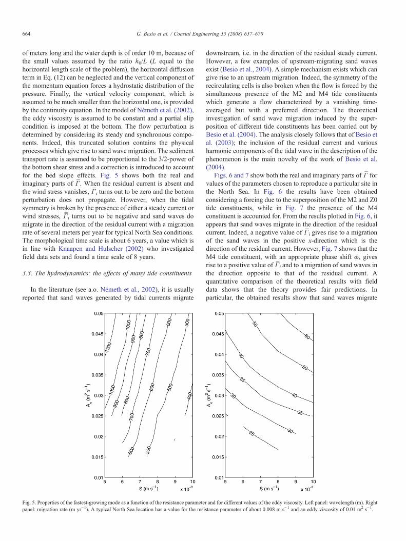
of meters long and the water depth is of order 10 m, because ofthe small values assumed by the ratio h0/L (L equal to thehorizontal length scale of the problem), the horizontal diffusionterm in Eq. (12) can be neglected and the vertical component ofthe momentum equation forces a hydrostatic distribution of thepressure. Finally, the vertical velocity component, which isassumed to be much smaller than the horizontal one, is providedby the continuity equation. In the model of Németh et al. (2002),the eddy viscosity is assumed to be constant and a partial slipcondition is imposed at the bottom. The flow perturbation isdetermined by considering its steady and synchronous compo-nents. Indeed, this truncated solution contains the physicalprocesses which give rise to sand wave migration. The sedimenttransport rate is assumed to be proportional to the 3/2-power ofthe bottom shear stress and a correction is introduced to accountfor the bed slope effects. Fig. 5 shows both the real andimaginary parts of Γ . When the residual current is absent andthe wind stress vanishes, Γ i turns out to be zero and the bottomperturbation does not propagate. However, when the tidalsymmetry is broken by the presence of either a steady current orwind stresses, Γ i turns out to be negative and sand waves domigrate in the direction of the residual current with a migrationrate of several meters per year for typical North Sea conditions.The morphological time scale is about 6 years, a value which isin line with Knaapen and Hulscher (2002) who investigatedfield data sets and found a time scale of 8 years.

3.3. The hydrodynamics: the effects of many tide constituents

In the literature (see a.o. Németh et al., 2002), it is usuallyreported that sand waves generated by tidal currents migrate

Fig. 5. Properties of the fastest-growing mode as a function of the resistance parametepanel: migration rate (m yr−1). A typical North Sea location has a value for the resi

downstream, i.e. in the direction of the residual steady current.However, a few examples of upstream-migrating sand wavesexist (Besio et al., 2004). A simple mechanism exists which cangive rise to an upstream migration. Indeed, the symmetry of therecirculating cells is also broken when the flow is forced by thesimultaneous presence of the M2 and M4 tide constituentswhich generate a flow characterized by a vanishing time-averaged but with a preferred direction. The theoreticalinvestigation of sand wave migration induced by the super-position of different tide constituents has been carried out byBesio et al. (2004). The analysis closely follows that of Besio etal. (2003); the inclusion of the residual current and variousharmonic components of the tidal wave in the description of thephenomenon is the main novelty of the work of Besio et al.(2004).

Figs. 6 and 7 show both the real and imaginary parts of Γ forvalues of the parameters chosen to reproduce a particular site inthe North Sea. In Fig. 6 the results have been obtainedconsidering a forcing due to the superposition of the M2 and Z0tide constituents, while in Fig. 7 the presence of the M4constituent is accounted for. From the results plotted in Fig. 6, itappears that sand waves migrate in the direction of the residualcurrent. Indeed, a negative value of Γ i gives rise to a migrationof the sand waves in the positive x-direction which is thedirection of the residual current. However, Fig. 7 shows that theM4 tide constituent, with an appropriate phase shift ϕ, givesrise to a positive value of Γ i and to a migration of sand waves inthe direction opposite to that of the residual current. Aquantitative comparison of the theoretical results with fielddata shows that the theory provides fair predictions. Inparticular, the obtained results show that sand waves migrate

r and for different values of the eddy viscosity. Left panel: wavelength (m). Rightstance parameter of about 0.008 m s−1 and an eddy viscosity of 0.01 m2 s−1.

Fig. 6. Influence of the steady component Z0 on the generation and migration of sand waves. Area SW1, transect P2 (see also Fig. 3): (a) dimensionless growth rate Γ r ,(b) dimensionless migration speed Γ i . Model parameters are: r =187, γ=0.23, µ=1.73, s=0.84 and U0m/U1m=0.043.

665G. Besio et al. / Coastal Engineering 55 (2008) 657–670

downstream or upstream depending on the strength and relativephase of the different tide constituents.

3.4. The hydro- and morphodynamics: a fully 3D model includingsuspended load and sediment transport due to the wind waves

A more refined model describing the generation andevolution of tidal sand waves from bottom perturbations of aflat sea bed subject to the action of tidal currents has been

Fig. 7. Generation and migration of sand waves in the area SW1 caused by Z0, M2 andspeed Γ i. Model parameters are: r=187, γ=0.23, µ=1.73, s=0.84, U0m/U1m=0.043

proposed by Besio et al. (2006). A horizontally two-dimensional basic flow forced by a tidal wave is consideredand Coriolis effects are taken into account since they affect tidepropagation. The basic flow is completely resolved also in thevertical direction from the free surface down to the sea bedwhere the no-slip condition is forced. Besio et al. (2006) notonly describe the sediment transport due to the tidal flow butalso the contribution which arises because of the presence ofwind waves which often coexist and have a large influence on

M4. Transect P2: (a) dimensionless growth rate Γ r, (b) dimensionless migration, U2m/U1m=0.145 and ϕ=60.7°.

Fig. 8. Prediction of the sand wave growth evaluated using the model (dashedline) and a linear trend analysis (dotted line), plotted against field measurements.

666 G. Besio et al. / Coastal Engineering 55 (2008) 657–670

the growth of bottom forms. For example Langhorne (1982)reports a significant decrease of the sand wave height (30%reduction) due to a storm. Also residual (steady) currents aretaken into account because their presence is essential inexplaining sand wave migration. Sediment is supposed tomove both as bed load and suspended load since field surveysshow that large amounts of sediment are set into suspension bythe stirring action of wind waves and then transported by tidalcurrents. Moreover, the effects of bottom slope on sedimenttransport are quantified by an accurate relationship.

The results obtained by Besio et al. (2006) agree well withfield observations. Indeed the strength of the tidal currents ableto trigger sand waves is well predicted as well as the maincharacteristics of the bottom forms (wavelength, orientation).The model can also predict the migration speed of sand waves,which is induced by residual currents or by the interaction ofdifferent tidal constituents.

3.5. Data assimilation: amplitude evolution model

The analyses summarized so far support the idea that sandwaves in tide-dominated coastal areas arise because of aninherent instability of the flat bottom configuration subject totidal currents.

The consequence of sand waves being free instabilities is thatthey tend to recover after dredging. This phenomenon has beenobserved by Katoh et al. (1998) who monitored the sea bed inthe Bisanseto Sea after a field of sand waves was topped off tokeep the navigation channel sufficiently deep. In particular,Katoh et al. (1998) showed that sand waves regenerate inseveral-years time. The costs of repeated dredging are high andthe responsible authorities want to minimize these costs.Therefore, it is crucial to know the rate at which the sandwaves regain their original shape. However, the linear analyses,previously described, neglect nonlinear effects. Hence, they canexplain the mechanism triggering the growth of the bottomforms forced by the propagation of a tidal wave and can predictsome of their characteristics (i.e. wavelengths, migration speedand initial growth rates), but they can predict neither theequilibrium attained by the bottom configuration nor the timewhich is required to attain this equilibrium shape.

Close to the critical conditions, the time development ofthe amplitude of the bottom perturbations including weakly-nonlinear effects could be predicted using the Landau andGinzburg amplitude equation, obtained by studying the self-interaction of the most unstable bottom perturbation of small butfinite amplitude, when the parameters are close to their criticalvalues. However, the analysis is tedious and lengthy. Hence,Knaapen and Hulscher (2002) choose a different approach toget an amplitude equation. They postulated that the system isclose to the critical conditions and determined the coefficientsof the amplitude equation and the initial amplitude of the bottomwaviness by using a genetic algorithm which fits the parametersof the model to the field data.

Because of the nonlinearity of the model, gradient searchalgorithms are not very effective (Fluodas and Pardalos, 1996).Therefore, Knaapen and Hulscher (2002) used a global

optimization routine. The algorithm is based on the evolutiontheory. The obtained results show that the proposedmodel gives agood representation of the process of sand wave growth in time.This makes it a useful tool for coastal management. Once themodel has been tuned, it can estimate the time development of theamplitude of sandwaves without expensive monitoring activities.Fig. 8 shows a comparison between the time developmentpredicted by Knaapen and Hulscher's (2002) model and the fielddata collected by Katoh et al. (1998). The good agreementbetween the theoretical results and the field surveys providessupport to Knaapen and Hulscher's (2002) analysis.

3.6. Data assimilation: amplitude evolution and migration

In the model developed by Knaapen and Hulscher (2002), thecoefficients appearing in the nonlinear amplitude equation areassumed to be real. Hence, the sand wave amplitude attains aconstant value after about a decade, but the bedforms do notmigrate. As they were interested in the water depth only this wasno limitation to them. Morelissen et al. (2003) applied the sameapproach to the safety of pipelines. For this application, theychose the coefficients to be complex, i.e. have an imaginary part.This introduces migration in the model. Since migrating sandwaves are asymmetric, Morelissen et al. (2003) also introducedhigher harmonics to the first order model of Knaapen andHulscher (2002). With these adaptations, a migrating bottomprofile can be characterized by few parameters. The values ofthese parameters are determined based on profiles observed in thefield using a global optimization technique. The analysis has beenapplied to both active and decommissioned offshore pipelines bycoupling their sand wave model to a model simulating self-lowering and self-burying of pipelines (PIPESIN— http://www.alkyon.nl/Tools/Pipesin.htm; Chen and Bijker, 2001). When apipeline is exposed on the seabed, it will influence the water flowlike any other object. Close to the pipeline, this leads to increasedflow velocities causing scour. The scouring will locally lower theseabed. If the flexibility of the pipeline is sufficient, the pipelinewill be lowered as well. This restores the undisturbed flow, and

667G. Besio et al. / Coastal Engineering 55 (2008) 657–670

the scour hole will fill, burying the pipeline again. Thiscombination of sand wave model and self-burying model canevaluate whether free spans will develop due to sand wavemigration or the self-lowering mechanism can compensate for thebed level changes due to migration. For a fairly small pipeline,the analysis showed that the latter was true, even in case ofdredging of the top 25% of the sand wave crests causingexposure of the pipelines over tens of meters (Fig. 9). Theregeneration of the sand waves, which occurs in about 7 yearsaccording to Knaapen and Hulscher (2002), together with theself-burying due to scour prevents the occurrence of free spans.This shows that dredging does not necessarily lead to largeexposure of the pipelines, which would increase the risk ofbuckling or breaking of the pipeline. If this would hold for morepipelines, this would allow for marine aggregate extraction insome of the pipeline areas, reducing the pressure onecologically more sensitive areas of shallow seas. However,these are only preliminary results on a small pipeline, and haveto be tested on more and larger pipelines.

3.7. Nonlinear analyses: finite amplitude sand waves

To investigate the intermediate-term behavior of sand waveshaving finite amplitudes, a numerical simulation model (2DV)is developed in Németh (2003). This model allows theevolutionary processes of sand waves after their initial evo-lution to be investigated.

The model is based on the 2DV shallow water equations,with a free water surface and a general bed load formula. Thewater movement is coupled to the sediment transport equationby a seabed evolution equation. The spatial discretisation isperformed by a spectral method based on Chebyshev poly-nomials. A fully implicit method is chosen for the discretisationin time. The model is validated by comparing the results forsmall-amplitude sand waves with the theoretical findings of alinear stability analysis (Németh et al., 2002). The results showthat the numerical model is able to reproduce the initialevolution of sand waves, as it was found in the linear stabilityanalysis (Németh, 2003).

Next, the simulation model was used to investigate thebehavior of offshore sand waves for finite values of theiramplitude (Németh and Hulscher, 2003 and Németh et al.,2007). A unidirectional steady current and a unidirectional block

Fig. 9. Predicted pipe and seabed levels in 2006, directly after dredging. The dashed liindicate areas of pipeline exposure. After Morelissen et al. (2003).

current simulating tidal motion were investigated. Initially, thesand waves develop exponentially, as follows from the linearstability analysis. Next, the growth rate diminishes, resulting inthe stabilization of the sand waves (see Fig. 10). The sand wavesreach a maximum height of about 10–30% of the average waterdepth in a matter of decades. The mechanism causing sandwaves to saturate is based on the increased importance, for largeramplitudes, of the principle that sediment is transported easierdownhill than uphill. This process counteracts the shear stress atthe seabed transporting sediment upward toward the crest.

For a unidirectional steady flow in an offshore setting, wefind sand waves with wavelengths in the order of hundreds ofmeters, based on linear theory, when the resistance at the seabedis relatively large. These sand waves migrate and becomeasymmetrical in the horizontal direction, as it is found for dunesin rivers. The migration rate of the sand waves decreasesslightly during their evolution. For a unidirectional blockcurrent slightly elongated troughs and sharp crests are found. Asensitivity analysis showed that the slope effects on thesediment transport play an important role. Furthermore, themagnitude of the resistance at the seabed and the eddy viscosityinfluence both the timescale and the height of the fully-developed sand waves. The orders of magnitude of the time andspatial scales coincide with observations made in the southernbight of the North Sea and Spain (Németh et al., 2007) andJapan (see also Knaapen and Hulscher, 2002).

Using this simulation model, the recovery of dredged sandwaves is investigated in Németh and Hulscher (2003). Sandwaves are able to recover after they are dredged (see alsoKnaapen and Hulscher, 2002). The timescale and resultingmaximum height depend on the amount of sand dredged andwhere the sand is dumped. The interested reader can find moredetails on the nonlinear model in Németh et al. (2006).

3.8. Linear evolution of sand wave packets

The existing models of sand wave formation, described inSections 3.1–3.4, typically describe the dynamics of wavypatterns of infinite spatial extent. Recently, Roos et al. (2005)have investigated how a local topographic disturbance of a flatseabed behaves subject to the linear instability mechanismassociated with sand wave formation. The time development ofsuch a disturbance can be expressed in terms of a Fourier

ne and the solid line indicate the top and bottom of the pipeline, while the squares

Fig. 10. Sand wave evolution and final profile for a block current. Left panel: development of the seabed (on the vertical axis in meters) as a function of time (yr). Theinitial height of the imposed sand wave is 0.05 m. It takes about 20 years to evolve from 10% to 90% of the saturation height. Right panel: final cross section of a sandwave (which is part of a sand wave pattern).

668 G. Besio et al. / Coastal Engineering 55 (2008) 657–670

integral containing the spectrum h~(αx, αy) of the local instan-

taneous bathymetry:

h x; y; sð Þ ¼ h0 þZ l

�l

Z l

�lh αx;αy; t� �

ei αxxþαyyð Þdαxdαy

¼ h0 þZ l

�l

Z l

�lhinit αx; αy

� �eΓ� αx;αyð Þtei αxxþαyyð Þdαxdαy þ c:c:

ð17Þ

in Eq. (17), h0 is the mean water depth, h~init(αx, αy) is the

Fourier spectrum of the initial bottom perturbation, in which

Fig. 11. Sketch of the components of a sand wave packet (right), which can be seen apattern of infinite spatial extent (centre). The latter migrates with the phase speed,The envelope also expands gradually with time. The top row shows the three-dimeet al., 2005).

every possibly wave vector (αx, αy) is represented and Γ (αx,αy)= Γ r+ iΓ i is the tide-averaged complex growth rate takenfrom any existing process-based sand wave formation model(see Eqs. (1) and (13)).

Roos et al. (2005) have proposed an analytical approach toapproximate the solution of this integral. They have considered alocal, three-dimensional perturbation with a Gaussian shape, andthey have approximated the dispersion relationship Γ(αx, αy)quadratically around the fastest-growing mode (αx,fgm, αy,fgm)(i.e., the mode for which the growth rate Γr attains its maximum).The proposed method is quick, insightful and performs well.

s the product of an envelope of Gaussian shape (left) and a migrating sand wavethe former with the group speed, both pertaining to the fastest-growing mode.nsional plots, the bottom row the values along y=0 (figure adapted from Roos

669G. Besio et al. / Coastal Engineering 55 (2008) 657–670

The local disturbance is shown to develop gradually into asand wave packet (Fig. 11), the horizontal area of whichincreases roughly linearly with time. The elevation at thepacket's center tends to increase, but initially it may decreasedepending on the spatial extent of the initial disturbance. In thecase of tidal asymmetry, the individual sand waves in the packetmigrate at the migration speed of the fastest-growing mode,whereas the packet's envelope moves at the group speed. Thetheoretical analysis is applied to trenches and pits, to showwhere the results differ from an earlier study of a timedevelopment of a trench in which sand wave dynamics wasignored.

4. Conclusions

The present review provides a description of some recentcontributions to the study of the mechanisms underlying theformation and evolution of large-scale sedimentary patternsobserved in the coastal region. These patterns are repetitive bothin space and in time. The wavelength of these bottom forms (sandwaves) is of a few hundreds of meters and the amplitude of a fewmeters. Sand waves are not static bedforms. Indeed, they migratewith a speed of a few meters per year. Even though simplifyingassumptions have been introduced, the theoretical models providefair predictions of the characteristics of the actual bottom formsand they can be used to solve practical problems.

Only the research carried out in the framework of theHUMOR project has been considered and the literature quotedabove is by no means exhaustive.

References

Allen, J.R.L., 1984. Development in Sedimentology. Elsevier.Besio, G., Blondeaux, P., Frisina, P., 2003. A note on tidally generated sand

waves. J.Fluid Mech. 485, 171–190.Besio, G., Blondeaux, P., Brocchini, M., Vittori, G., 2004. On the modelling of

sand wave migration. J. Geophys. Res. Oceans 109 (C4). doi:10.1029/2002JC001622 C04018.

Besio, G., Blondeaux, P., Vittori, G., 2006. On the formation of sand waves andsand banks. J. Fluid Mech. 557, 1–27. doi:10.1017/S0022112006009256.

Blondeaux, P., 1990. Sand ripples under sea waves. Part I. Ripple formation.J. Fluid Mech. 218, 1–17.

Blondeaux, P., 2001. Mechanics of coastal forms. Annu. Rev. Fluid Mech. 33,339–370.

Chen, Z., Bijker, R., 2001. Interactions of offshore pipelines and dynamic seabed.In: Li, G. (Ed.), Proceedings XXIX IAHR Congress, pp. 128–133. Beijing.

Colombini, M., Seminara, G., Tubino, M., 1987. Finite-amplitude alternate bars.J. Fluid Mech. 181, 213–232.

Dodd,N., Blondeaux, P., Calvete, D., De Swart, H., Falques,A., Hulscher, S.J.M.H.,Rozynski, G., Vittori, G., 2003. The role of stability methods for understandingthe morphodynamical behaviour of coastal systems. Cont. Shelf Res. 19,849–865.

Engelund, F., 1970. Instability of erodible beds. J. Fluid Mech. 42, 225–244.Fluodas, C.A., Pardalos, P.M., 1996. State of Art in Global Optimization. Kluver

Academic Publisher, Dordrecht. 651 pp.Gerkema, T., 2000. A linear stability analysis of tidally generated sand waves.

J. Fluid Mech. 417, 303–322.Hulscher, S., Garlan, T., Idier, D., 2004. In: Hulscher, S., Garlan, T., Idier, D.

(Eds.), Proceedings of: Marine Sand-Wave and River Dunes Dynamics II,International Workshop, April 1–2. University of Twente, the Netherlands,p. 352.

Hulscher, S.J.M.H., 1996. Tidal-induced large-scale regular bedform patterns ina three-dimensional shallowwater model. J. Geophys. Res. Oceans 101 (C9),20727–20744.

Hulscher, S.J.M.H., Van de Brink, G.M., 2001. Comparison between predictedand observed sand waves and sand banks in the North Sea. J. Geophys. Res.Oceans 106 (C5), 9327–9338.

Idier D. 2002. Dynamics of continental shelf sandbanks and sand waves: in situmeasurements and numerical modeling. PhD Thesis, National PolytechnicalInstitute, Toulouse Est., France, 314 pp.

Idier, D., Ehrhold, A., Garlan, T., 2002. Morphodynamics of an underseasandwave of the Dover Straits C.R. Geosciences 334, 1079–1085.

Idier, D., Astruc, D., Hulscher, S.J.M.H., 2004. Influence of bed roughness ondune and megaripple generation. Geophys. Res. Lett. (ISSN: 0094-8276)L13214, 31. doi:10.1029/2004GL019969.

Katoh, K., Kume, H., Kuroki, K., Hasegawa, J., 1998. The development of sandwaves and the maintenance of navigation channels in the Bisanseto Sea.Coastal Eng. '98. ASCE, Reston, VA, pp. 3490–3502.

Knaapen, M.A.F., 2005. Measuring sand wave migration in the field.Comparison of different data sources and an error analysis. J. Geophys.Res.-Earth Surface 110 (F4).

Knaapen, M.A.F., Hulscher, S.J.M.H., 2002. Regeneration of sand waves afterdredging. Coast. Eng. 46, 277–289.

Knaapen, M.A.F., Hulscher, S.J.M.H., Vriend, H.J. de, Stolk, A., 2001. A newtype of sea bed waves. Geophys. Res. Lett. 28 (7), 1323–1326.

Knaapen, M.A.F., Hulscher, S.J.M.H., Tiessen, M.C.H., van den Berg, J., 2005.Using a sand wave model for optimal monitoring of a navigation depth. In:Parker, G., Garcia, M.H. (Eds.), Proceedings forth IAHR Symposium onRiver, Coastal and Estuarine Morphodynamics 2005, Urbana, Illinois, USA,pp. 999–1007. RCEM 2005 IAHR.

Komarova, N.L., Hulscher, S.J.M.H., 2000. Linear instability mechanism forsand wave formation. J. Fluid Mech. 413, 219–246.

Langhorne, D.N., 1982. A study of the dynamics of a marine sand wave.Sedimentology 29, 571–594.

Le Bot, S., Trentesaux, A., 2004. Types of internal structure and externalmorphology of submarine dunes under the influence of tide- and wind-drivenprocesses (Dover Strait, northern France). Mar. Geol. 211, 143–168.

Le Bot, 2001. Morphodynamics of submarine dunes under the influence of tidesand storms. PhD Thesis, University of Lille 1, France. , 272 pp.

Meyer-Peter, E., Müller, R., 1948. Formulas for bedload transport. III Conf. Int.Assoc. Hydraul. Res. Stockholm, Sweden.

Morelissen, R., Hulscher, S.J.M.H., Knaapen,M.A.F., Németh, A.A., Bi-jker, R.,2003. Mathematical modelling of sand wave migration and the interactionwith pipelines. Coast. Eng. 48, 197–209.

Németh A.A. 2003. Modelling offshore sand waves. Ph.D. Thesis, University ofTwente, The Netherlands.

Németh, A.A., Hulscher, S.J.M.H., 2003. Finite amplitude sandwaves in shallowseas. In: Sánchez-Arcilla, A., Bateman, A. (Eds.), Proceedings Third IAHRSymposium on River, Coastal and Estuarine Morphodynamics 2003,Barcelona, Spain. ISBN: 90-805649-6-6, pp. 435–444. RCEM 2003 IAHR.

Németh, A.A., Hulscher, S.J.M.H., de Vriend, H.J., 2002. Modelling sand wavemigration in shallow shelf seas. Cont. Shelf Res. 22, 2795–2806.

Németh, A.A., Hulscher, S.J.M.H., Vriend, H.J. de, 2003. Offshore sand wavedynamics, engineering problems and future solutions. Pipeline Gas J. 230,67–69.

Németh, A.A., Hulscher, S.J.M.H., Damme, R.M.J. van, 2006. Simulatingoffshore sand waves. Coast. Eng. 53, 265–275.

Németh, A.A., Hulscher, S.J.M.H., Damme, R.M.J. van, 2007. Modellingoffshore sandwave evolution. Cont. Shelf Res. 27 (5), 713–728 (ISSN 0278-4343).

Roos, P.C., Blondeaux, P., Hulscher, S.J.M.H., Vittori, G., 2005. Linearevolution of sandwave packets. J. Geophys. Res. 110, F04S14. doi:10.1029/2004JF000196.

Schielen, R., Doelman, A., de Swart, H.E., 1992. On the nonlinear dynamics offree bars in straight channels. J. Fluid Mech. 252, 325–356.

Seminara, G., 1998. Stability and morphodynamics. Mecc. 33, 59–99.Sleath, J.F.M., 1976. On rolling grain ripples. J. Hydraul. Res. 14, 69–81.Stride, A.H., 1982. Offshore Tidal Sands (Processes and Deposits). Chapman

and Hall.

670 G. Besio et al. / Coastal Engineering 55 (2008) 657–670

Trentesaux, A., Garlan, T. (Eds.), 2000. Marine Sandwave Dynamics (Dynamiquedes dunes sous-marines). Proceedings of an International Workshop, March23–24 2000. University of Lille 1, France. ISBN: 2-11-088263-8, p. 240.

Van der Veen, H.H., Hulscher, S.J.M.H., Knaapen, M.A.F., 2006. Grain sizedependency in the occurrence of sand waves. Ocean Dynamics 56, 228–234(ISSN 1616-7341). doi:10.1007/s10236-005-0049-7.

Vittori, G., 1989. Nonlinear viscous oscillatory flow over a small amplitudewavy wall. J. Hydraul. Res. 27, 267–280.

Vittori, G., Blondeaux, P., 1990. Sand ripples under sea waves. Part II. Finite-amplitude development. J. Fluid Mech. 218, 19–39.