The Montgomery ladder on binary elliptic curves

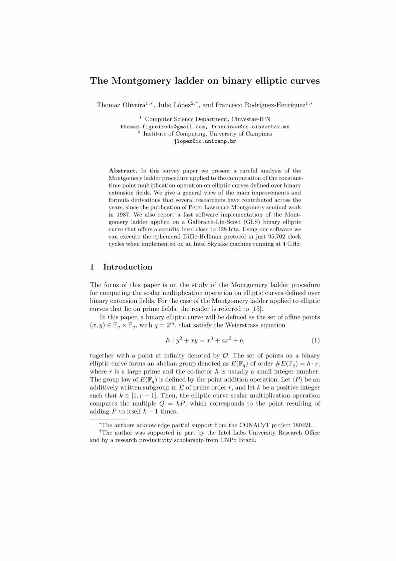
The Montgomery ladder on binary elliptic curves

Thomaz Oliveira1,∗, Julio Lopez2,†, and Francisco Rodrıguez-Henrıquez1,∗

1 Computer Science Department, [email protected], [email protected]

2 Institute of Computing, University of [email protected]

Abstract. In this survey paper we present a careful analysis of theMontgomery ladder procedure applied to the computation of the constant-time point multiplication operation on elliptic curves defined over binaryextension fields. We give a general view of the main improvements andformula derivations that several researchers have contributed across theyears, since the publication of Peter Lawrence Montgomery seminal workin 1987. We also report a fast software implementation of the Mont-gomery ladder applied on a Galbraith-Lin-Scott (GLS) binary ellipticcurve that offers a security level close to 128 bits. Using our software wecan execute the ephemeral Diffie-Hellman protocol in just 95,702 clockcycles when implemented on an Intel Skylake machine running at 4 GHz.

1 Introduction

The focus of this paper is on the study of the Montgomery ladder procedurefor computing the scalar multiplication operation on elliptic curves defined overbinary extension fields. For the case of the Montgomery ladder applied to ellipticcurves that lie on prime fields, the reader is referred to [15].

In this paper, a binary elliptic curve will be defined as the set of affine points(x, y) ∈ Fq × Fq, with q = 2m, that satisfy the Weierstrass equation

E : y2 + xy = x3 + ax2 + b, (1)

together with a point at infinity denoted by O. The set of points on a binaryelliptic curve forms an abelian group denoted as E(Fq) of order #E(Fq) = h · r,where r is a large prime and the co-factor h is usually a small integer number.The group law of E(Fq) is defined by the point addition operation. Let 〈P 〉 be anadditively written subgroup in E of prime order r, and let k be a positive integersuch that k ∈ [1, r − 1]. Then, the elliptic curve scalar multiplication operationcomputes the multiple Q = kP , which corresponds to the point resulting ofadding P to itself k − 1 times.

∗The authors acknowledge partial support from the CONACyT project 180421.†The author was supported in part by the Intel Labs University Research Office

and by a research productivity scholarship from CNPq Brazil.

In [52], Peter Lawrence Montgomery famously presented a procedure thatallows one to compute an elliptic curve scalar multiplication using only the x-coordinate of the involved points. Although Montgomery conceived his ladder foraccelerating Lenstra’s ECM factorization algorithm [44], in this paper we willaddress the application of this procedure for achieving efficient elliptic-curve-based cryptography.

The key algorithmic idea of the Montgomery ladder is that given the x-coordinates of the points kP and (k + 1)P , one can apply specialized additionand doubling formulas to compute the x-coordinates of the points (2k + 1)Pand 2kP. Moreover, Montgomery presented a special form of elliptic curves thatlie on large characteristic fields, now known as Montgomery curves, which wereparticularly well suited for computing the scalar multiplication at a cost of aboutsix field multiplications and four squarings per ladder step. The case for binaryelliptic curves however, was not addressed in [52].

In fact, a few years after its publication, the convenience of using the Mont-gomery ladder procedure for binary elliptic curves remained unclear. For in-stance, due to the lack of an efficient projective coordinate formulation of thebinary elliptic curve arithmetic required at each ladder step, the Montgomeryladder was deemed to be inefficient in [1,49].

It was only one decade later, after the publication of Montgomery’s landmarkpaper that it became apparent that this approach could be as well applied to thebinary elliptic curve case efficiently. In [46], Lopez and Dahab presented compactprojective formulae for the elliptic curve arithmetic of the Montgomery ladder,by representing the points as P = (X,−, Z), in an analogous way as Montgomerydid it ten years before in [52]. This projective point representation avoids all thecostly field multiplicative inversions. It was shown in [46] that the computationalcost of a binary elliptic curve ladder step is of five field multiplications, onemultiplication by a constant, four squarings and three additions.

Furthermore, the authors of [46] presented a formula that permits to recoverthe y-coordinate of the points involved in the Montgomery ladder procedure.This y-coordinate retrieval formula opened the door for the full computation ofelliptic curve scalar multiplications using the Montgomery ladder procedure.3

Binary GLS curvesInspired in the Galbraith-Lin-Scott elliptic curves introduced in [22], Hankerson,Karabina and Menezes reported in [27] a family of binary GLS curves definedover the quadratic field Fq2 , with q = 2m. GLS curves are cryptographicallyinteresting mainly because they come equipped with a two-dimensional endo-morphism. By carefully choosing the elliptic curve parameters a, b of Eq. (1),the authors of [27] found instances of GLS curves with an almost-prime grouporder of the form #Ea,b(Fq2) = hr, with h = 2 and where r is a (2m − 1)-bitprime number.

3The analogous of this recovering formula has been recently applied in the contextof hyperelliptic curves [13,60].

Taking advantage of the two-dimensional endomorphism ψ associated toGLS curves, a point multiplication can be computed using the Gallant-Lambert-Vanstone (GLV) approach presented in [25] as

Q = kP = k1P + k2ψ(P ) = k1P + k2 · δP, (2)

where the subscalars |k1|, |k2| ≈ n/2, with n = dlog2(r)e, can be found by usinglattice techniques [22].

λ coordinates for binary curvesIn λ-affine coordinates [55] the points are represented as P = (x, λ), with x 6= 0and λ = x+ y

x . The λ-affine form of the Weierstrass Eq. (1) becomes

E : (λ2 + λ+ a)x2 = x4 + 1.

λ-point representation provides efficient point addition, doubling and halv-ing formulas. In [55], Oliveira et al. applied this coordinate system into a bi-nary GLS curve defined over the quadratic extension of the binary field F2127 .When implemented on a Haswell processor, this approach permits to computea constant-time variable-point multiplication in just 48, 312 clock cycles [56],which is the current speed-record for an elliptic curve designed to offer about128 bits of security level.

Security of Binary elliptic curvesThe Pollard’s Rho algorithm can be used to solve the Discrete Logarithm Prob-lem (DLP) over an elliptic curve subgroup of a prime order r with an averagerunning time given as 4

3

√r2 [21]. In the case of binary elliptic curves, by ap-

plying the negation map, an extra small improvement acceleration (which re-duces the attack complexity by less than 2 bits) to the above estimate can beachieved [7,67]. Using the Pollard’s Rho algorithm, the authors of [7] were able tocompute the current elliptic curve DLP record computation on a binary ellipticcurve defined over the field F2127 .

Given an ordinary binary elliptic curve satisfying Eq.(1), the Gaudry-Hess-Smart (GHS) attack [16,24,26,28,50] attempts to find an algebraic curve C of arelatively small genus g, such that the the target elliptic curve group is containedin the Jacobian of C. In this case, the original elliptic curve discrete logarithmproblem can be transferred into the Jacobian of C defined over F2l , with l|m. Ifthe genus of such a curve C is not too large, nor too short, then the DLP wouldbe easier to solve in that Jacobian, due to the availability of a relatively efficientindex-calculus strategy for that group.

In general however, the GHS strategy is difficult to implement because of thelarge genus of suitable curves C. This difficulty is so serious, that the authorsof [26,50] reported that the GHS attack fails, i.e., the Pollard’s rho attack is moreeffective, for all binary elliptic curves defined over F2m, where m ∈ [160, 600] isa prime number. Further, in [47], it was proved that the GHS attack fails formost of the composite extensions in the range m ∈ [160, 600].

New lines of research for solving the DLP over binary curves were presentedby Semaev in 2004 [63], by introducing summation-polynomial methods (some-times also referred as Semaev’s polynomials). Since then, several researchershave attempted to attack the DLP on binary elliptic curves using this ap-proach [23,19,64]. However, the current status of these attempts are based onGrobner basis assumptions that are still not well understood, which in somecases have led to contradictory behaviors, even for tiny experiments [29].

For a comprehensive survey of recent progress in the computation of the el-liptic curve discrete problem in characteristic two, the reader is referred to thepaper by Galbraith and Gaudry [21]. All in all, it is not hyperbolic to claim thatat the moment the most ominous threat to the security of binary elliptic curvesis the announced advent of quantum computers, only that this peril is sharedby all elliptic-curve based cryptography.

Aim of this paperThe aim of this paper is two-fold. First, we would like to present a recountof some of the main research findings for the Montgomery ladder applied onbinary elliptic curves. We also present a short summary of some of the mostrelevant software and hardware implementations reported for this procedure.Second, we report a state-of-the-art software implementation of the Montgomeryladder on a GLS binary curve that can take advantage of pre-computation whenthe base point is known. Using this approach, we can execute the ephemeralDiffie-Hellman protocol in just 95,702 clock cycles when implemented on anIntel Skylake machine running at 4 GHz.

The remainder of this survey is organized as follows. In §2, we describe theMontgomery ladder and by using a division polynomial approach, we re-discoverthe point addition and doubling formulas required for performing a Montgomeryladder step. We also re-discover the y-coordinate retrieval formula as it was orig-inally reported in [46]. In §3 we describe a Montgomery ladder procedures thatadmit off-line pre-computation, which was a long-standing open problem thatwas solved in [54] by Oliveira et al. In §4, we report a software implementa-tion of a Montgomery ladder point multiplication that targets the Intel Skylakeprocessor. In §5 we present a selection of the most interesting implementationsof the Montgomery ladder point multiplication in software and hardware plat-forms; in this section, we also present the useful common-Z trick, that permitsvaluable area savings for light hardware implementations, and a brief descrip-tion of multi-dimensional Montgomery ladders. Finally, we draw our concludingremarks in §6.

2 Montgomery ladders on binary elliptic curves

We begin this section by describing the Montgomery ladder algorithm. Then,we use the division polynomial technique, which was suggested by Victor Millerin [51], in order to re-discover the point addition and doubling formulas, as wellas the y-coordinate retrieval formula, as they were reported in [46].

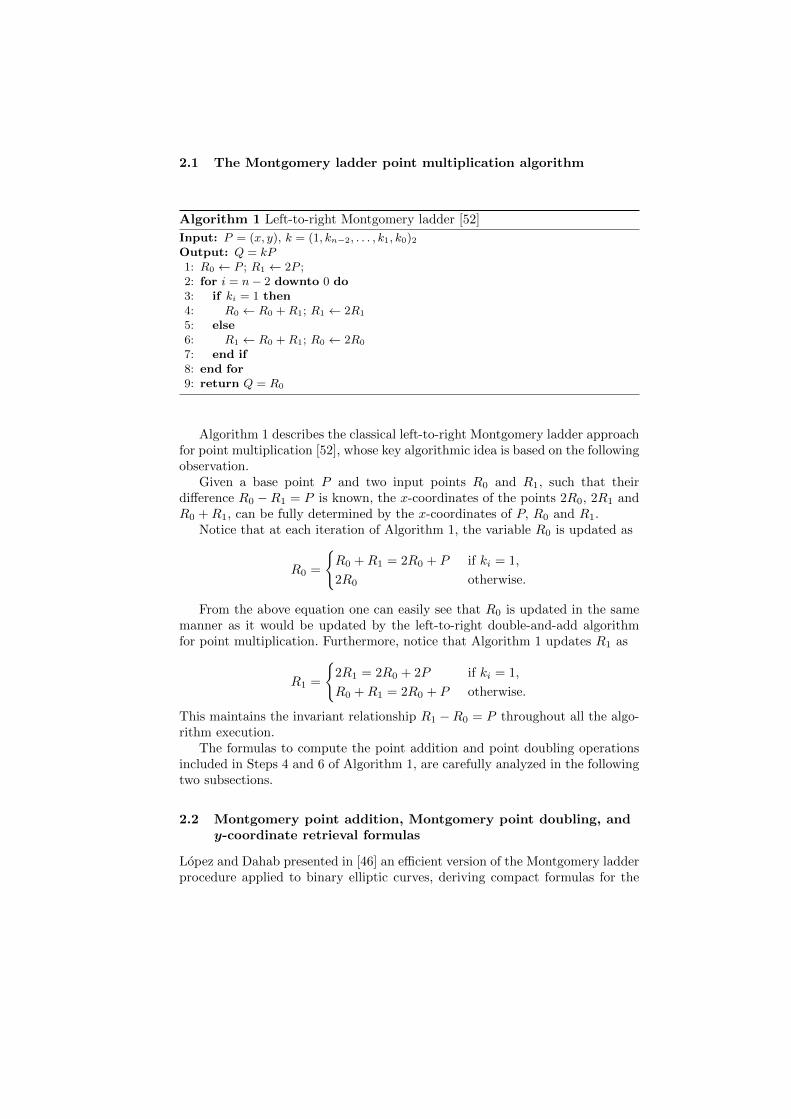
2.1 The Montgomery ladder point multiplication algorithm

Algorithm 1 Left-to-right Montgomery ladder [52]

Input: P = (x, y), k = (1, kn−2, . . . , k1, k0)2Output: Q = kP1: R0 ← P ; R1 ← 2P ;2: for i = n− 2 downto 0 do3: if ki = 1 then4: R0 ← R0 +R1; R1 ← 2R1

5: else6: R1 ← R0 +R1; R0 ← 2R0

7: end if8: end for9: return Q = R0

Algorithm 1 describes the classical left-to-right Montgomery ladder approachfor point multiplication [52], whose key algorithmic idea is based on the followingobservation.

Given a base point P and two input points R0 and R1, such that theirdifference R0 −R1 = P is known, the x-coordinates of the points 2R0, 2R1 andR0 +R1, can be fully determined by the x-coordinates of P, R0 and R1.

Notice that at each iteration of Algorithm 1, the variable R0 is updated as

R0 =

{R0 +R1 = 2R0 + P if ki = 1,

2R0 otherwise.

From the above equation one can easily see that R0 is updated in the samemanner as it would be updated by the left-to-right double-and-add algorithmfor point multiplication. Furthermore, notice that Algorithm 1 updates R1 as

R1 =

{2R1 = 2R0 + 2P if ki = 1,

R0 +R1 = 2R0 + P otherwise.

This maintains the invariant relationship R1 −R0 = P throughout all the algo-rithm execution.

The formulas to compute the point addition and point doubling operationsincluded in Steps 4 and 6 of Algorithm 1, are carefully analyzed in the followingtwo subsections.

2.2 Montgomery point addition, Montgomery point doubling, andy-coordinate retrieval formulas

Lopez and Dahab presented in [46] an efficient version of the Montgomery ladderprocedure applied to binary elliptic curves, deriving compact formulas for the

point addition and point doubling operations of Algorithm 1. Moreover, the au-thors of [46] presented for the first time a retrieval formula that allows to recoverthe y-coordinate of the points involved in the Montgomery ladder procedure.

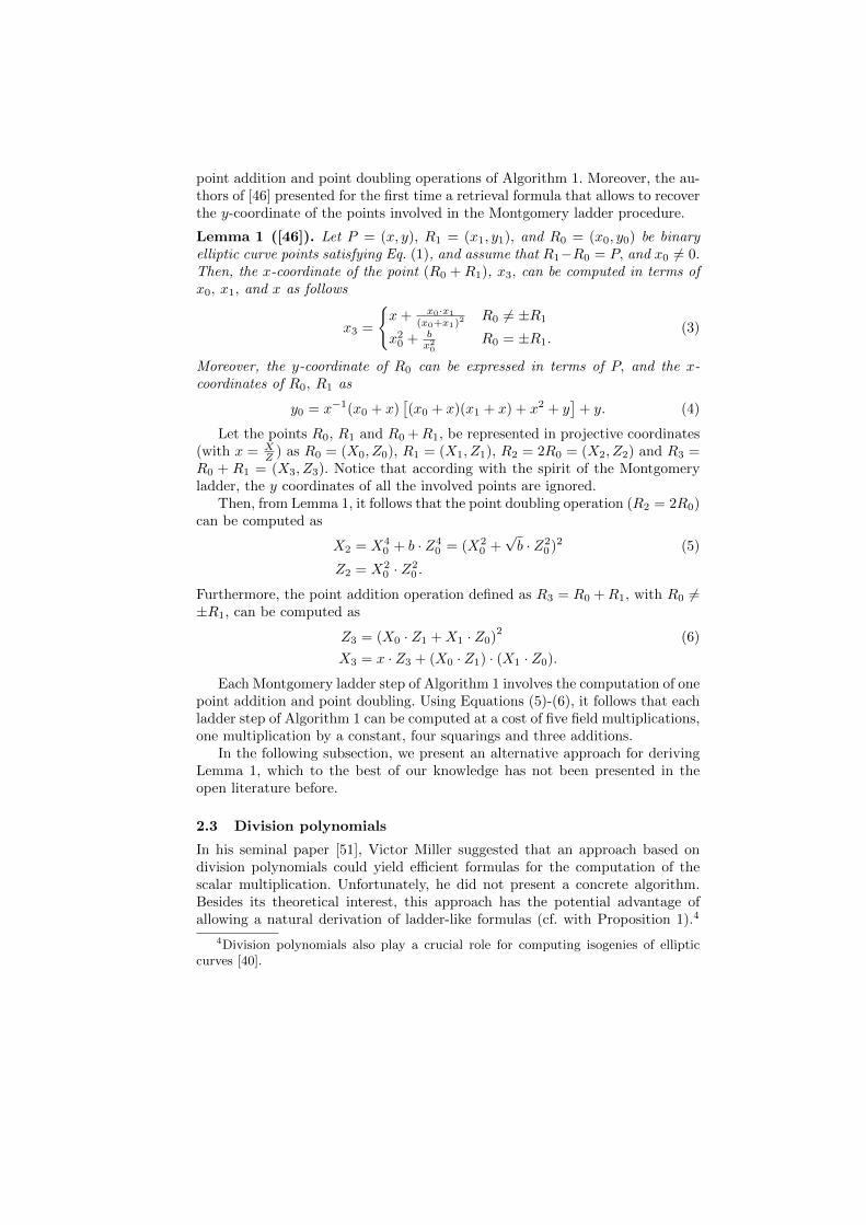
Lemma 1 ([46]). Let P = (x, y), R1 = (x1, y1), and R0 = (x0, y0) be binaryelliptic curve points satisfying Eq. (1), and assume that R1−R0 = P, and x0 6= 0.Then, the x-coordinate of the point (R0 +R1), x3, can be computed in terms ofx0, x1, and x as follows

x3 =

{x+ x0·x1

(x0+x1)2 R0 6= ±R1

x20 + bx20

R0 = ±R1.(3)

Moreover, the y-coordinate of R0 can be expressed in terms of P, and the x-coordinates of R0, R1 as

y0 = x−1(x0 + x)[(x0 + x)(x1 + x) + x2 + y

]+ y. (4)

Let the points R0, R1 and R0 +R1, be represented in projective coordinates(with x = X

Z ) as R0 = (X0, Z0), R1 = (X1, Z1), R2 = 2R0 = (X2, Z2) and R3 =R0 + R1 = (X3, Z3). Notice that according with the spirit of the Montgomeryladder, the y coordinates of all the involved points are ignored.

Then, from Lemma 1, it follows that the point doubling operation (R2 = 2R0)can be computed as

X2 = X40 + b · Z4

0 = (X20 +√b · Z2

0 )2 (5)

Z2 = X20 · Z2

0 .

Furthermore, the point addition operation defined as R3 = R0 +R1, with R0 6=±R1, can be computed as

Z3 = (X0 · Z1 +X1 · Z0)2

(6)

X3 = x · Z3 + (X0 · Z1) · (X1 · Z0).

Each Montgomery ladder step of Algorithm 1 involves the computation of onepoint addition and point doubling. Using Equations (5)-(6), it follows that eachladder step of Algorithm 1 can be computed at a cost of five field multiplications,one multiplication by a constant, four squarings and three additions.

In the following subsection, we present an alternative approach for derivingLemma 1, which to the best of our knowledge has not been presented in theopen literature before.

2.3 Division polynomials

In his seminal paper [51], Victor Miller suggested that an approach based ondivision polynomials could yield efficient formulas for the computation of thescalar multiplication. Unfortunately, he did not present a concrete algorithm.Besides its theoretical interest, this approach has the potential advantage ofallowing a natural derivation of ladder-like formulas (cf. with Proposition 1).4

4Division polynomials also play a crucial role for computing isogenies of ellipticcurves [40].

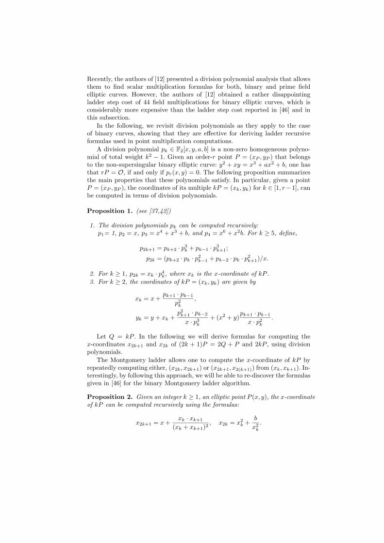
Recently, the authors of [12] presented a division polynomial analysis that allowsthem to find scalar multiplication formulas for both, binary and prime fieldelliptic curves. However, the authors of [12] obtained a rather disappointingladder step cost of 44 field multiplications for binary elliptic curves, which isconsiderably more expensive than the ladder step cost reported in [46] and inthis subsection.

In the following, we revisit division polynomials as they apply to the caseof binary curves, showing that they are effective for deriving ladder recursiveformulas used in point multiplication computations.

A division polynomial pk ∈ F2[x, y, a, b] is a non-zero homogeneous polyno-mial of total weight k2 − 1. Given an order-r point P = (xP , yP ) that belongsto the non-supersingular binary elliptic curve: y2 + xy = x3 + ax2 + b, one hasthat rP = O, if and only if pr(x, y) = 0. The following proposition summarizesthe main properties that these polynomials satisfy. In particular, given a pointP = (xP , yP ), the coordinates of its multiple kP = (xk, yk) for k ∈ [1, r−1], canbe computed in terms of division polynomials.

Proposition 1. (see [37,42])

1. The division polynomials pk can be computed recursively:p1= 1, p2 = x, p3 = x4 + x3 + b, and p4 = x6 + x2b. For k ≥ 5, define,

p2k+1 = pk+2 · p3k + pk−1 · p3k+1;

p2k = (pk+2 · pk · p2k−1 + pk−2 · pk · p2k+1)/x.

2. For k ≥ 1, p2k = xk · p4k, where xk is the x-coordinate of kP .

3. For k ≥ 2, the coordinates of kP = (xk, yk) are given by

xk = x+pk+1 · pk−1

p2k,

yk = y + xk +p2k+1 · pk−2x · p3k

+ (x2 + y)pk+1 · pk−1x · p2k

.

Let Q = kP . In the following we will derive formulas for computing thex-coordinates x2k+1 and x2k of (2k + 1)P = 2Q + P and 2kP , using divisionpolynomials.

The Montgomery ladder allows one to compute the x-coordinate of kP byrepeatedly computing either, (x2k, x2k+1) or (x2k+1, x2(k+1)) from (xk, xk+1). In-terestingly, by following this approach, we will be able to re-discover the formulasgiven in [46] for the binary Montgomery ladder algorithm.

Proposition 2. Given an integer k ≥ 1, an elliptic point P (x, y), the x-coordinateof kP can be computed recursively using the formulas:

x2k+1 = x+xk · xk+1

(xk + xk+1)2, x2k = x2k +

b

x2k.

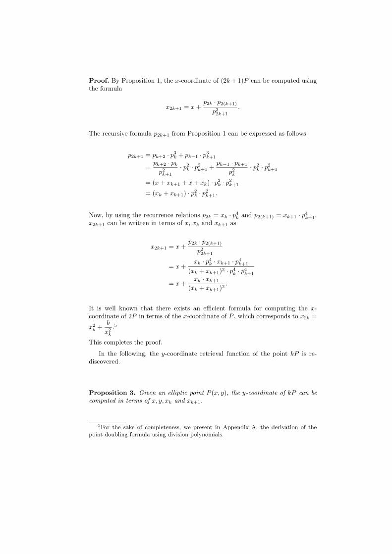
Proof. By Proposition 1, the x-coordinate of (2k+ 1)P can be computed usingthe formula

x2k+1 = x+p2k · p2(k+1)

p22k+1

.

The recursive formula p2k+1 from Proposition 1 can be expressed as follows

p2k+1 = pk+2 · p3k + pk−1 · p3k+1

=pk+2 · pkp2k+1

· p2k · p2k+1 +pk−1 · pk+1

p2k· p2k · p2k+1

= (x+ xk+1 + x+ xk) · p2k · p2k+1

= (xk + xk+1) · p2k · p2k+1.

Now, by using the recurrence relations p2k = xk · p4k and p2(k+1) = xk+1 · p4k+1,x2k+1 can be written in terms of x, xk and xk+1 as

x2k+1 = x+p2k · p2(k+1)

p22k+1

= x+xk · p4k · xk+1 · p4k+1

(xk + xk+1)2 · p4k · p4k+1

= x+xk · xk+1

(xk + xk+1)2.

It is well known that there exists an efficient formula for computing the x-coordinate of 2P in terms of the x-coordinate of P , which corresponds to x2k =

x2k +b

x2k.5

This completes the proof.

In the following, the y-coordinate retrieval function of the point kP is re-discovered.

Proposition 3. Given an elliptic point P (x, y), the y-coordinate of kP can becomputed in terms of x, y, xk and xk+1.

5For the sake of completeness, we present in Appendix A, the derivation of thepoint doubling formula using division polynomials.

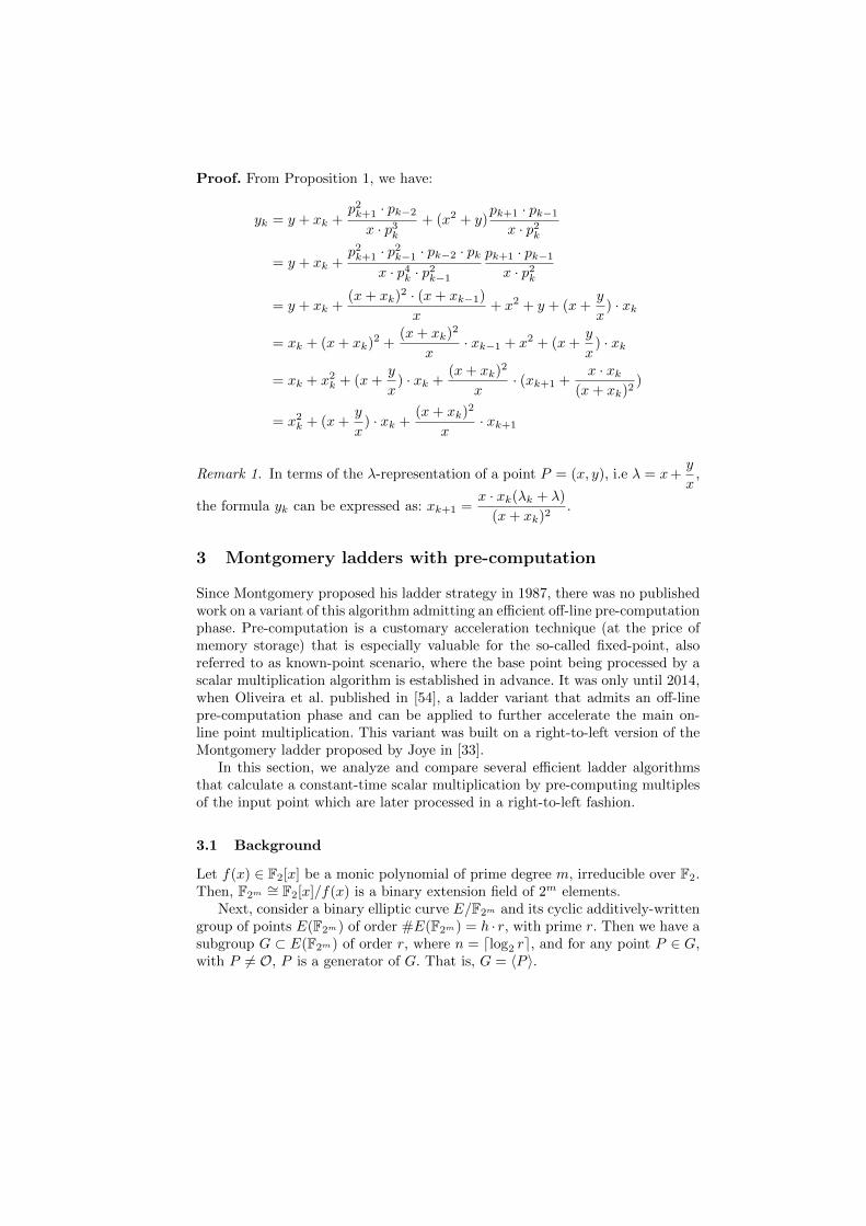
Proof. From Proposition 1, we have:

yk = y + xk +p2k+1 · pk−2x · p3k

+ (x2 + y)pk+1 · pk−1x · p2k

= y + xk +p2k+1 · p2k−1 · pk−2 · pk

x · p4k · p2k−1pk+1 · pk−1x · p2k

= y + xk +(x+ xk)2 · (x+ xk−1)

x+ x2 + y + (x+

y

x) · xk

= xk + (x+ xk)2 +(x+ xk)2

x· xk−1 + x2 + (x+

y

x) · xk

= xk + x2k + (x+y

x) · xk +

(x+ xk)2

x· (xk+1 +

x · xk(x+ xk)2

)

= x2k + (x+y

x) · xk +

(x+ xk)2

x· xk+1

Remark 1. In terms of the λ-representation of a point P = (x, y), i.e λ = x+y

x,

the formula yk can be expressed as: xk+1 =x · xk(λk + λ)

(x+ xk)2.

3 Montgomery ladders with pre-computation

Since Montgomery proposed his ladder strategy in 1987, there was no publishedwork on a variant of this algorithm admitting an efficient off-line pre-computationphase. Pre-computation is a customary acceleration technique (at the price ofmemory storage) that is especially valuable for the so-called fixed-point, alsoreferred to as known-point scenario, where the base point being processed by ascalar multiplication algorithm is established in advance. It was only until 2014,when Oliveira et al. published in [54], a ladder variant that admits an off-linepre-computation phase and can be applied to further accelerate the main on-line point multiplication. This variant was built on a right-to-left version of theMontgomery ladder proposed by Joye in [33].

In this section, we analyze and compare several efficient ladder algorithmsthat calculate a constant-time scalar multiplication by pre-computing multiplesof the input point which are later processed in a right-to-left fashion.

3.1 Background

Let f(x) ∈ F2[x] be a monic polynomial of prime degree m, irreducible over F2.Then, F2m

∼= F2[x]/f(x) is a binary extension field of 2m elements.Next, consider a binary elliptic curve E/F2m and its cyclic additively-written

group of points E(F2m) of order #E(F2m) = h · r, with prime r. Then we have asubgroup G ⊂ E(F2m) of order r, where n = dlog2 re, and for any point P ∈ G,with P 6= O, P is a generator of G. That is, G = 〈P 〉.

The scalar multiplication algorithms discussed in this section receive as inputa generator point P ∈ G, and an n-bit scalar k ∈ {1, . . . , r − 1} and return thepoint Q = kP , which, as mentioned in the introduction of this article, is theprocess of adding P to itself k − 1 times.

3.2 A right-to-left Montgomery ladder

In addition to the traditional left-to-right approach presented in Algorithm 1, onecan compute the Montgomery ladder by processing the scalar k from the least tothe most significant bit. This method is denominated Montgomery right-to-leftdouble-and-add and it is shown in Algorithm 2.

Algorithm 2 Montgomery right-to-left double-and-add [33]

Input: P = (x, y) ∈ G, k = (kn−1, kn−2, . . . , k1, k0)2 ∈ Zr

Output: Q = khP

1: Initialization: Select an order-h point S ∈ E(F2m) \G2: R0 ← P , R1 ← S, R2 ← P − S3: for i← 0 to n− 1 do4: if ki = 1 then5: R1 ← R0 +R1

6: else7: R2 ← R0 +R2

8: end if9: R0 ← 2R0

10: end for11: return Q = hR1

The rationale of Algorithm 2 can be explained as follows. At the beginningof the iteration i, with i ∈ {0, . . . , n− 1}, R0 stores the point 2iP , 6 which willbe added to the accumulator R1 if the scalar digit ki is equal to one.

As discussed in Section 2, in order to perform the Montgomery addition (Step5), we need to know the difference between the accumulator R1 and the pointR0. However, unlike the classical left-to-right ladder, this difference is not fixed,but may vary at each iteration; more specifically, it will change whenever thedigit ki is equal to zero. For that reason, we have to occasionally update andstore this varying difference in the point R2 (Step 7).

In other words, if the bit ki is one, R0 is added to the accumulator R1 andtheir difference does not need to be updated because the addition is compensatedin Step 9 as 2R0 = R0 +R0. On the other hand, if the digit ki is zero, R0 is notadded to the accumulator. As a consequence, the difference between R1 and R0

increases by R0, and R2 must be updated.

6According to Algorithm 2, at the end of the iteration n−1, 2nP is assigned to R0.The point 2nP is never used in the unknown-point scenario, therefore this assignationcan be avoided in practical implementations.

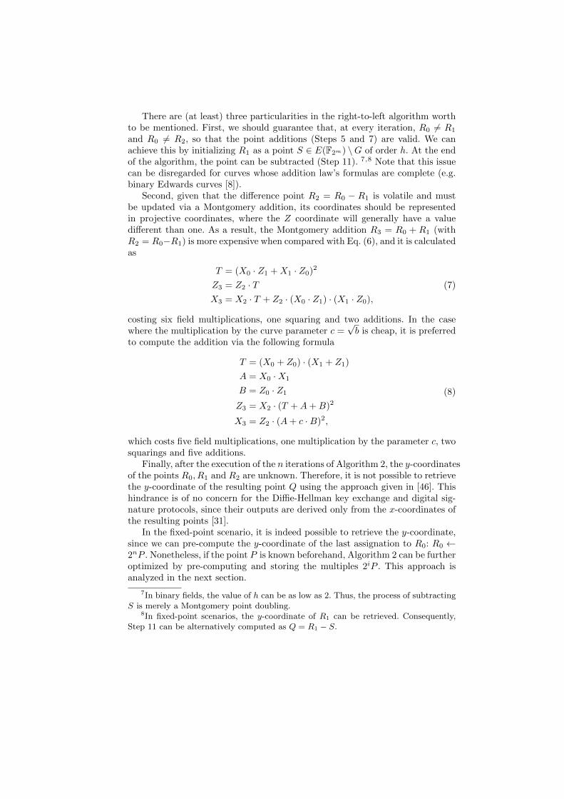
There are (at least) three particularities in the right-to-left algorithm worthto be mentioned. First, we should guarantee that, at every iteration, R0 6= R1

and R0 6= R2, so that the point additions (Steps 5 and 7) are valid. We canachieve this by initializing R1 as a point S ∈ E(F2m) \G of order h. At the endof the algorithm, the point can be subtracted (Step 11). 7,8 Note that this issuecan be disregarded for curves whose addition law’s formulas are complete (e.g.binary Edwards curves [8]).

Second, given that the difference point R2 = R0 − R1 is volatile and mustbe updated via a Montgomery addition, its coordinates should be representedin projective coordinates, where the Z coordinate will generally have a valuedifferent than one. As a result, the Montgomery addition R3 = R0 + R1 (withR2 = R0−R1) is more expensive when compared with Eq. (6), and it is calculatedas

T = (X0 · Z1 +X1 · Z0)2

Z3 = Z2 · TX3 = X2 · T + Z2 · (X0 · Z1) · (X1 · Z0),

(7)

costing six field multiplications, one squaring and two additions. In the casewhere the multiplication by the curve parameter c =

√b is cheap, it is preferred

to compute the addition via the following formula

T = (X0 + Z0) · (X1 + Z1)

A = X0 ·X1

B = Z0 · Z1

Z3 = X2 · (T +A+B)2

X3 = Z2 · (A+ c ·B)2,

(8)

which costs five field multiplications, one multiplication by the parameter c, twosquarings and five additions.

Finally, after the execution of the n iterations of Algorithm 2, the y-coordinatesof the points R0, R1 and R2 are unknown. Therefore, it is not possible to retrievethe y-coordinate of the resulting point Q using the approach given in [46]. Thishindrance is of no concern for the Diffie-Hellman key exchange and digital sig-nature protocols, since their outputs are derived only from the x-coordinates ofthe resulting points [31].

In the fixed-point scenario, it is indeed possible to retrieve the y-coordinate,since we can pre-compute the y-coordinate of the last assignation to R0: R0 ←2nP . Nonetheless, if the point P is known beforehand, Algorithm 2 can be furtheroptimized by pre-computing and storing the multiples 2iP . This approach isanalyzed in the next section.

7In binary fields, the value of h can be as low as 2. Thus, the process of subtractingS is merely a Montgomery point doubling.

8In fixed-point scenarios, the y-coordinate of R1 can be retrieved. Consequently,Step 11 can be alternatively computed as Q = R1 − S.

3.3 Montgomery ladders with pre-computation

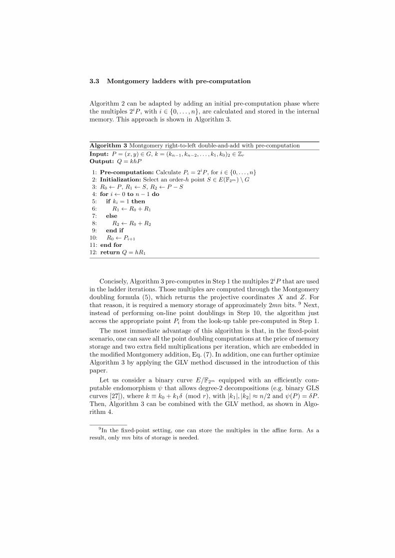
Algorithm 2 can be adapted by adding an initial pre-computation phase wherethe multiples 2iP , with i ∈ {0, . . . , n}, are calculated and stored in the internalmemory. This approach is shown in Algorithm 3.

Algorithm 3 Montgomery right-to-left double-and-add with pre-computation

Input: P = (x, y) ∈ G, k = (kn−1, kn−2, . . . , k1, k0)2 ∈ Zr

Output: Q = khP

1: Pre-computation: Calculate Pi = 2iP , for i ∈ {0, . . . , n}2: Initialization: Select an order-h point S ∈ E(F2m) \G3: R0 ← P , R1 ← S, R2 ← P − S4: for i← 0 to n− 1 do5: if ki = 1 then6: R1 ← R0 +R1

7: else8: R2 ← R0 +R2

9: end if10: R0 ← Pi+1

11: end for12: return Q = hR1

Concisely, Algorithm 3 pre-computes in Step 1 the multiples 2iP that are usedin the ladder iterations. Those multiples are computed through the Montgomerydoubling formula (5), which returns the projective coordinates X and Z. Forthat reason, it is required a memory storage of approximately 2mn bits. 9 Next,instead of performing on-line point doublings in Step 10, the algorithm justaccess the appropriate point Pi from the look-up table pre-computed in Step 1.

The most immediate advantage of this algorithm is that, in the fixed-pointscenario, one can save all the point doubling computations at the price of memorystorage and two extra field multiplications per iteration, which are embedded inthe modified Montgomery addition, Eq. (7). In addition, one can further optimizeAlgorithm 3 by applying the GLV method discussed in the introduction of thispaper.

Let us consider a binary curve E/F2m equipped with an efficiently com-putable endomorphism ψ that allows degree-2 decompositions (e.g. binary GLScurves [27]), where k ≡ k0 + k1δ (mod r), with |k1|, |k2| ≈ n/2 and ψ(P ) = δP .Then, Algorithm 3 can be combined with the GLV method, as shown in Algo-rithm 4.

9In the fixed-point setting, one can store the multiples in the affine form. As aresult, only mn bits of storage is needed.

Algorithm 4 Montgomery 2-GLV right-to-left double-and-add with pre-computation

Input: P = (x, y) ∈ G, k ∈ Zr

Output: Q = khP

1: Pre-computation: Calculate Pi = 2iP , for i ∈ {0, . . . , n2}

2: Initialization: Decompose the scalar k as k ≡ k0 + k1δ (mod r) via the GLVmethod. Select an order-h point S ∈ E(F2m) \G

3: R0 ← P , R1,j ← S, R2,j ← P − S, for j ∈ {0, 1}4: for i← 0 to n

2− 1 do

5: for j ← 0 to 1 do6: if ki,j = 1 then7: R1,j ← R0 +R1,j

8: else9: R2,j ← R0 +R2,j

10: end if11: end for12: R0 ← Pi+1

13: end for14: return Q = (hR1,0) + ψ(hR1,1) 10

Here, the number of point doublings were reduced by half, which resultsin less computing time and less required storage resources, since only nm bitsof memory space are necessary. Note that even in the unknown-point scenario,one can profit from this algorithm, by exchanging a smaller number of pointdoublings with a more expensive point addition. The feasibility of this trade willbe evaluated in Section 3.6.

In the remaining of this section it is shown how to use the point halvingoperation to reduce the cost of the right-to-left point additions.

3.4 The point halving operation

In 1999, Knudsen [36] and Schroppel [61,62] proposed the application of thepoint halving operation to compute scalar multiplications. Given a point P ∈E(F2m), the point halving operation consists of computing a point R such thatP = 2R. The interested reader is referred to [3,20,54,55] for a discussion on howto implement point halvings efficiently.

Let k ∈ Zr be a scalar of n bits. Then, in order to perform a scalar multiplica-tion with point halvings, k must be first manipulated as k′ = 2n−1k mod r. Con-sequently, k ≡

∑ni=1 k

′n−i/2

i−1 (mod r) and therefore, kP =∑n

i=1 k′n−i(

P2i−1 ).

This implies that we can compute Q = kP by performing consecutive point halv-ings on P . This method is called halve-and-add and is presented in Algorithm5.

Computing the scalar multiplication via point halvings is usually more ef-ficient than the traditional double-and-add algorithm. This is because we need

10If the order h is prime, then one can return instead the pointQ = h(R1,0+ψ(R1,1)).

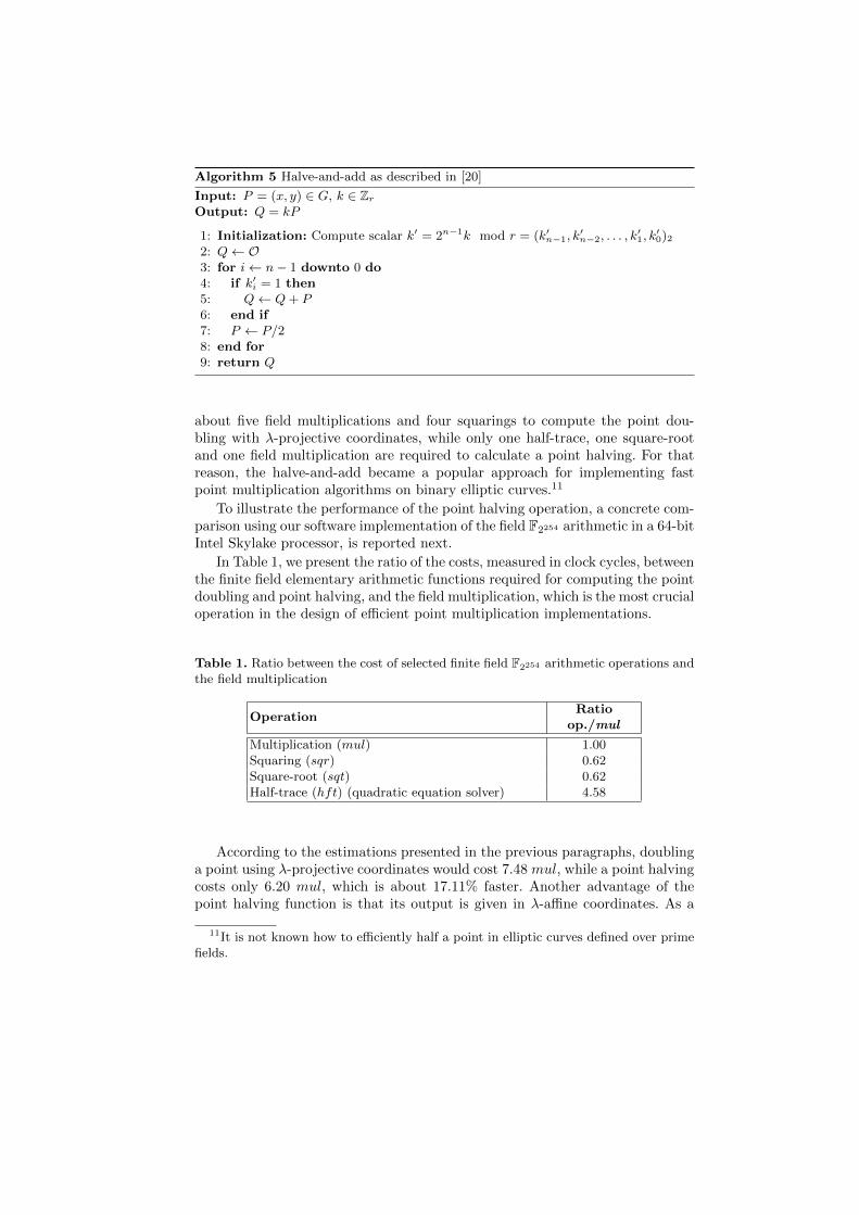
Algorithm 5 Halve-and-add as described in [20]


Output: Q = kP

1: Initialization: Compute scalar k′ = 2n−1k mod r = (k′n−1, k′n−2, . . . , k

′1, k′0)2

2: Q← O3: for i← n− 1 downto 0 do4: if k′i = 1 then5: Q← Q+ P6: end if7: P ← P/28: end for9: return Q

about five field multiplications and four squarings to compute the point dou-bling with λ-projective coordinates, while only one half-trace, one square-rootand one field multiplication are required to calculate a point halving. For thatreason, the halve-and-add became a popular approach for implementing fastpoint multiplication algorithms on binary elliptic curves.11

To illustrate the performance of the point halving operation, a concrete com-parison using our software implementation of the field F2254 arithmetic in a 64-bitIntel Skylake processor, is reported next.

In Table 1, we present the ratio of the costs, measured in clock cycles, betweenthe finite field elementary arithmetic functions required for computing the pointdoubling and point halving, and the field multiplication, which is the most crucialoperation in the design of efficient point multiplication implementations.

Table 1. Ratio between the cost of selected finite field F2254 arithmetic operations andthe field multiplication

OperationRatio

op./mul

Multiplication (mul) 1.00Squaring (sqr) 0.62Square-root (sqt) 0.62Half-trace (hft) (quadratic equation solver) 4.58

According to the estimations presented in the previous paragraphs, doublinga point using λ-projective coordinates would cost 7.48 mul, while a point halvingcosts only 6.20 mul, which is about 17.11% faster. Another advantage of thepoint halving function is that its output is given in λ-affine coordinates. As a

11It is not known how to efficiently half a point in elliptic curves defined over primefields.

result, we can compute faster point additions in right-to-left point multiplicationalgorithms, since the Z-coordinates of the points P/2i will all be equal to 1.

3.5 An efficient halve-and-add Montgomery ladder

Applying the point halving to the Montgomery ladder context is not straight-forward. The main reason being the fact that the only known efficient formulasfor computing R = P/2 assume that the input point is given in affine coordi-nates. On the other hand, Montgomery ladder algorithms manipulate accumula-tor points in projective coordinates in order to avoid the costly field multiplica-tive inversions.

The authors of [53] partially solved this problem by converting the accumula-tor point from projective to affine representation at every ladder step. Neverthe-less, this approach is too expensive, since it requires one inversion per iteration,with an associated cost of about 29.38 mul, which becomes prohibitive for mostscenarios.

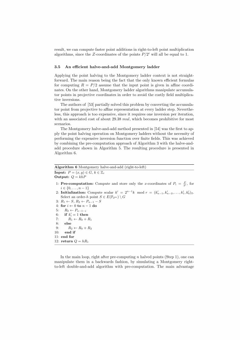
The Montgomery halve-and-add method presented in [54] was the first to ap-ply the point halving operation on Montgomery ladders without the necessity ofperforming the expensive inversion function over finite fields. This was achievedby combining the pre-computation approach of Algorithm 3 with the halve-and-add procedure shown in Algorithm 5. The resulting procedure is presented inAlgorithm 6.

Algorithm 6 Montgomery halve-and-add (right-to-left)


Output: Q = khP

1: Pre-computation: Compute and store only the x-coordinates of Pi = P2i, for

i ∈ {0, . . . , n− 1}2: Initialization: Compute scalar k′ = 2n−1k mod r = (k′n−1, k

′n−2, . . . , k

′1, k′0)2.

Select an order-h point S ∈ E(F2m) \G3: R1 ← S, R2 ← Pn−1 − S4: for i← 0 to n− 1 do5: R0 ← Pn−1−i

6: if k′i = 1 then7: R1 ← R0 +R1

8: else9: R2 ← R0 +R2

10: end if11: end for12: return Q = hR1

In the main loop, right after pre-computing n halved points (Step 1), one canmanipulate them in a backwards fashion, by simulating a Montgomery right-to-left double-and-add algorithm with pre-computation. The main advantage

of this approach is that the coordinates of R0 = Pi are represented in λ-affinecoordinates, that is, Z0 is always equal to 1. As a result, the Montgomery additionformula (see Eq. (7)) can be simplified as shown the following equation:

T = (X0 · Z1 +X1)2

Z3 = Z2 · TX3 = X2 · T + Z2 · (X0 · Z1) ·X1,

(9)

which costs five field multiplications, one squaring and two additions. Similarly,Eq. (9) leads to a faster addition, if the multiplication by the elliptic curveparameter b is cheap.

Given that R0 is represented in λ-affine coordinates, we can retrieve the R1 y-coordinate in the fixed and variable-point scenarios. At the end of the algorithm,we only have to compute R0 ← 2P 12 and apply the retrieval function of [46].

The Montgomery halve-and-add algorithm can be combined with the 2-GLVdecomposition method as well. In that case, the number of pre-computed halvedpoints would be reduced by a factor of two. Given that the halved points arerepresented in λ-affine coordinates, the required pre-computing memory spaceof this approach is of only mn

2 bits.

3.6 Comparison

In this subsection, we compare the algorithms and operations previously dis-cussed. First, in Table 2, we show an analysis of the costs of different point arith-metic operations used in Montgomery ladders in terms of the field arithmeticfunctions described in Table 1 and the field multiplication. The field additionswere disregarded since, for binary fields, this operation can be implemented viaan exclusive-or logical operator, which is nearly free of cost in high-end desktoparchitectures. 13

At first glance, Table 2 shows that substituting Montgomery point doublingsby point halvings is not a good idea, since the latter costs 2.74 mul more thanthe former. However, in the 2-GLV method, both operations are shared in the“parallel” computation of k0P and k1P (see Algorithm 4). Thus, since only n

2of such operations are required, we can conclude that the cost per iteration ofDBL and HLV in the 2-GLV algorithms are 1.73 mul and 3.10 mul, respec-tively. Now, the HLV is only 1.37 mul more expensive than DBL. Given thatthe Montgomery addition for halve-and-add (ADM) is cheaper than the pointaddition for double-and-add (ADF ) by 15.11%, we can expect similar timingsfor the two approaches.

In Table 3, we report the cost estimates, in terms of the point operations listedin the previous table and also in terms of field multiplications, for the ladderalgorithms described in this section considering the variable-point scenario.

12In Algorithm 6, R0 is updated after R1 and R2.13The latency and the throughput of the vector instruction pxor in current desktop

architectures is of 1 and 0.33 clock cycles, respectively [32].

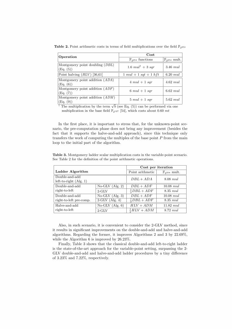
Table 2. Point arithmetic costs in terms of field multiplications over the field F2254

OperationCost

F2254 functions F2254 mult.

Montgomery point doubling (DBL)(Eq. (5))

1.6 mul† + 3 sqr 3.46 mul

Point halving (HLV ) [36,61] 1 mul + 1 sqt + 1 hft 6.20 mul

Montgomery point addition (ADA)(Eq. (6))

4 mul + 1 sqr 4.62 mul

Montgomery point addition (ADF )(Eq. (7))


Montgomery point addition (ADM )(Eq. (9))


† The multiplication by the term√b (see Eq. (5)) can be performed via one

multiplication in the base field F2127 [54], which costs about 0.60 mt

In the first place, it is important to stress that, for the unknown-point sce-nario, the pre-computation phase does not bring any improvement (besides thefact that it supports the halve-and-add approach), since this technique onlytransfers the work of computing the multiples of the base point P from the mainloop to the initial part of the algorithm.

Table 3. Montgomery ladder scalar multiplication costs in the variable-point scenario.See Table 2 for the definition of the point arithmetic operations.

Ladder AlgorithmCost per iteration

Point arithmetic F2254 mult.

Double-and-addleft-to-right (Alg. 1)

DBL+ADA 8.08 mul

Double-and-addright-to-left

No-GLV (Alg. 2) DBL+ADF 10.08 mul

2-GLV12DBL+ADF 8.35 mul

Double-and-addright-to-left pre-comp.

No-GLV (Alg. 3) DBL+ADF 10.08 mul2-GLV (Alg. 4) 1

2DBL+ADF 8.35 mul

Halve-and-addright-to-left

No-GLV (Alg. 6) HLV +ADM 11.82 mul

2-GLV12HLV +ADM 8.72 mul

Also, in such scenario, it is convenient to consider the 2-GLV method, sinceit results in significant improvements on the double-and-add and halve-and-addalgorithms. Regarding the former, it improves Algorithms 2 and 3 by 22.69%,while the Algorithm 6 is improved by 26.23%.

Finally, Table 3 shows that the classical double-and-add left-to-right ladderis the state-of-the-art approach for the variable-point setting, surpassing the 2-GLV double-and-add and halve-and-add ladder procedures by a tiny differenceof 3.23% and 7.22%, respectively.

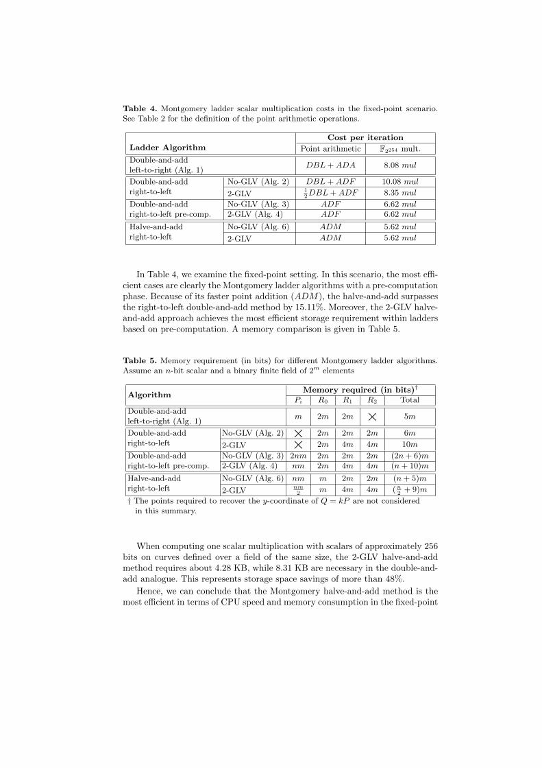
Table 4. Montgomery ladder scalar multiplication costs in the fixed-point scenario.See Table 2 for the definition of the point arithmetic operations.

Ladder AlgorithmCost per iteration

Point arithmetic F2254 mult.


DBL+ADA 8.08 mul


No-GLV (Alg. 2) DBL+ADF 10.08 mul

2-GLV12DBL+ADF 8.35 mul


No-GLV (Alg. 3) ADF 6.62 mul2-GLV (Alg. 4) ADF 6.62 mul


No-GLV (Alg. 6) ADM 5.62 mul

2-GLV ADM 5.62 mul

In Table 4, we examine the fixed-point setting. In this scenario, the most effi-cient cases are clearly the Montgomery ladder algorithms with a pre-computationphase. Because of its faster point addition (ADM), the halve-and-add surpassesthe right-to-left double-and-add method by 15.11%. Moreover, the 2-GLV halve-and-add approach achieves the most efficient storage requirement within laddersbased on pre-computation. A memory comparison is given in Table 5.

Table 5. Memory requirement (in bits) for different Montgomery ladder algorithms.Assume an n-bit scalar and a binary finite field of 2m elements

AlgorithmMemory required (in bits)†

Pi R0 R1 R2 Total


m 2m 2m × 5m


No-GLV (Alg. 2) × 2m 2m 2m 6m

2-GLV × 2m 4m 4m 10m


No-GLV (Alg. 3) 2nm 2m 2m 2m (2n+ 6)m2-GLV (Alg. 4) nm 2m 4m 4m (n+ 10)m


No-GLV (Alg. 6) nm m 2m 2m (n+ 5)m

2-GLVnm2

m 4m 4m (n2

+ 9)m

† The points required to recover the y-coordinate of Q = kP are not consideredin this summary.

When computing one scalar multiplication with scalars of approximately 256bits on curves defined over a field of the same size, the 2-GLV halve-and-addmethod requires about 4.28 KB, while 8.31 KB are necessary in the double-and-add analogue. This represents storage space savings of more than 48%.

Hence, we can conclude that the Montgomery halve-and-add method is themost efficient in terms of CPU speed and memory consumption in the fixed-point

scenario. In the variable-point setting, the classical double-and-add left-to-rightalgorithm is still the most convenient alternative.

4 A software implementation of Montgomeryladder-based elliptic curve protocols

In this section, software implementations for different 128-bit secure Montgomeryladder scalar multiplication algorithms on binary GLS curves are presented. 14

4.1 Field and curve parameters

The base field F2127∼= F2[x]/(f(x)) was generated using the irreducible polyno-

mial,f(x) = x127 + x63 + 1.

The quadratic field F2254∼= F2127 [u]/(g(u)) is constructed by means of the degree-

2 irreducible polynomial,g(u) = u2 + u+ 1.

In the following, the parameters of the binary GLS curve

Ea,b/F2254 : y2 + xy = x3 + ax2 + b,

are presented. All the polynomials representing the field elements will be giventhrough integer hexadecimal numbers:

a = 0x1u,

b = 0x54045144410401544101540540515101.

The rationale for selecting the b parameter was based on the X-coordinatecomputation in the Montgomery projective doubling R3 = 2R1. Let us recallthat its formula requires one multiplication by the square-root of b :

X3 = X41 + b · Z4

1 = (X21 +√b · Z2

1 )2.

Since our software architecture provides a 64-bit carry-less multiplier, weselected b such that its square-root

√b = 0xE2DA921E91E38DD1 is also of a size

of 64 bits. Thanks to this choice, we could save one carry-less multiplication andmany logical operations in the field multiplication by this constant.

Lastly, our base point P belongs to a sub-group G ⊂ Ea,b(F2254) of primeorder r of about 253 bits given by

r = 0x1FFFFFFFFFFFFFFFFFFFFFFFFFFFFFFF

A6B89E49D3FECD828CA8D66BF4B88ED5.

14The implementation to be described here closely follows the one presented byOliveira et al. in [54].

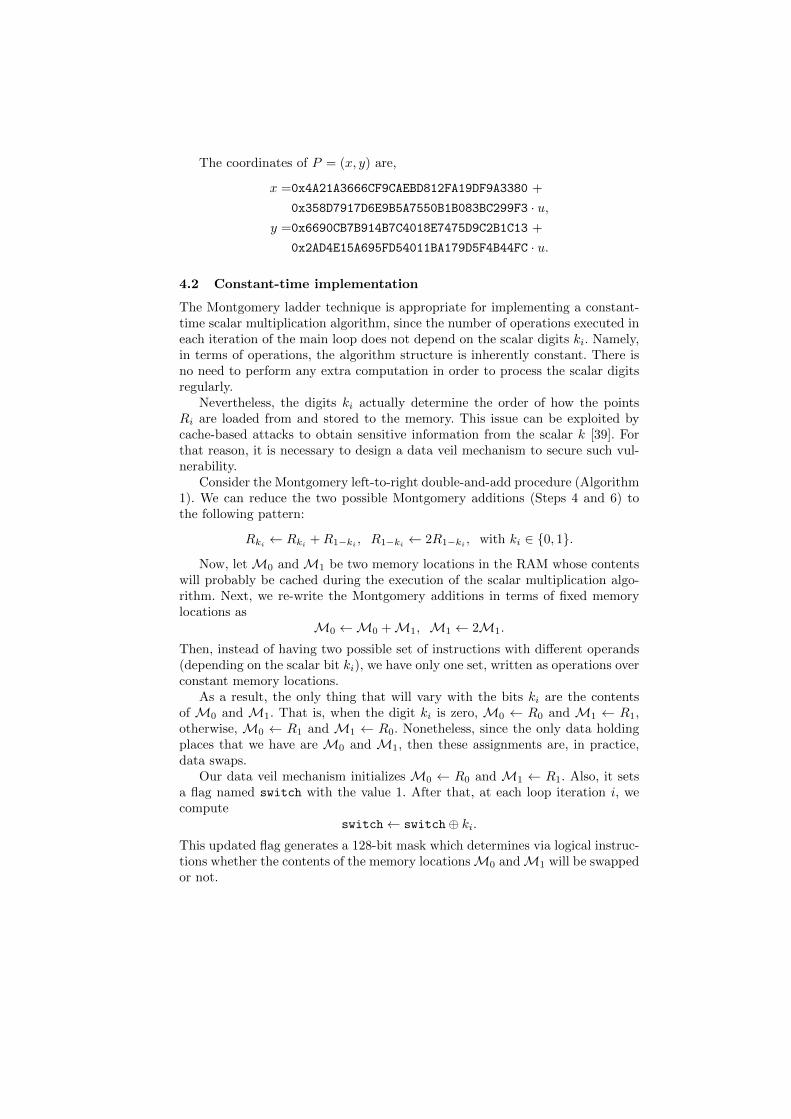
The coordinates of P = (x, y) are,

x =0x4A21A3666CF9CAEBD812FA19DF9A3380 +

0x358D7917D6E9B5A7550B1B083BC299F3 · u,y =0x6690CB7B914B7C4018E7475D9C2B1C13 +

0x2AD4E15A695FD54011BA179D5F4B44FC · u.

4.2 Constant-time implementation

The Montgomery ladder technique is appropriate for implementing a constant-time scalar multiplication algorithm, since the number of operations executed ineach iteration of the main loop does not depend on the scalar digits ki. Namely,in terms of operations, the algorithm structure is inherently constant. There isno need to perform any extra computation in order to process the scalar digitsregularly.

Nevertheless, the digits ki actually determine the order of how the pointsRi are loaded from and stored to the memory. This issue can be exploited bycache-based attacks to obtain sensitive information from the scalar k [39]. Forthat reason, it is necessary to design a data veil mechanism to secure such vul-nerability.

Consider the Montgomery left-to-right double-and-add procedure (Algorithm1). We can reduce the two possible Montgomery additions (Steps 4 and 6) tothe following pattern:

Rki ← Rki +R1−ki , R1−ki ← 2R1−ki , with ki ∈ {0, 1}.

Now, letM0 andM1 be two memory locations in the RAM whose contentswill probably be cached during the execution of the scalar multiplication algo-rithm. Next, we re-write the Montgomery additions in terms of fixed memorylocations as

M0 ←M0 +M1, M1 ← 2M1.

Then, instead of having two possible set of instructions with different operands(depending on the scalar bit ki), we have only one set, written as operations overconstant memory locations.

As a result, the only thing that will vary with the bits ki are the contentsof M0 and M1. That is, when the digit ki is zero, M0 ← R0 and M1 ← R1,otherwise, M0 ← R1 and M1 ← R0. Nonetheless, since the only data holdingplaces that we have are M0 and M1, then these assignments are, in practice,data swaps.

Our data veil mechanism initializes M0 ← R0 and M1 ← R1. Also, it setsa flag named switch with the value 1. After that, at each loop iteration i, wecompute

switch← switch⊕ ki.This updated flag generates a 128-bit mask which determines via logical instruc-tions whether the contents of the memory locationsM0 andM1 will be swappedor not.

The procedure is described in Algorithm 7. Here, [α, β] denotes a 128-bitvector register that stores two 64-bit values α and β. Also, the symbols ∧ and⊕ represents the logical instructions ‘and’ (pand) and exclusive-or (pxor), re-spectively. The logical conjunction with negation (¬) of the first operand isimplemented through the instruction pandn.

Algorithm 7 Data veil procedure

Input: Memory locations M0,M1, switch flag, bit kiOutput: The contents of the points R0, R1 stored in M0,M1 according to ki1: one ← [0x1, 0x1]2: switch ← switch ⊕ ki3: mask ← [switch, switch] - one4: M0 ← (mask ∧M0)⊕ (¬mask ∧M1)5: M1 ← (mask ∧M1)⊕ (¬mask ∧M0)6: Proceed to the Step 6 or 4 of Algorithm 1

For right-to-left Montgomery ladders, the data veil countermeasure is similar.The only difference is that, in these algorithms, the addition operation is fixedas

M0 ← R0 +M0.

Then, the content of one of the points R1, R2 is temporarily stored in an auxiliarymemory location.

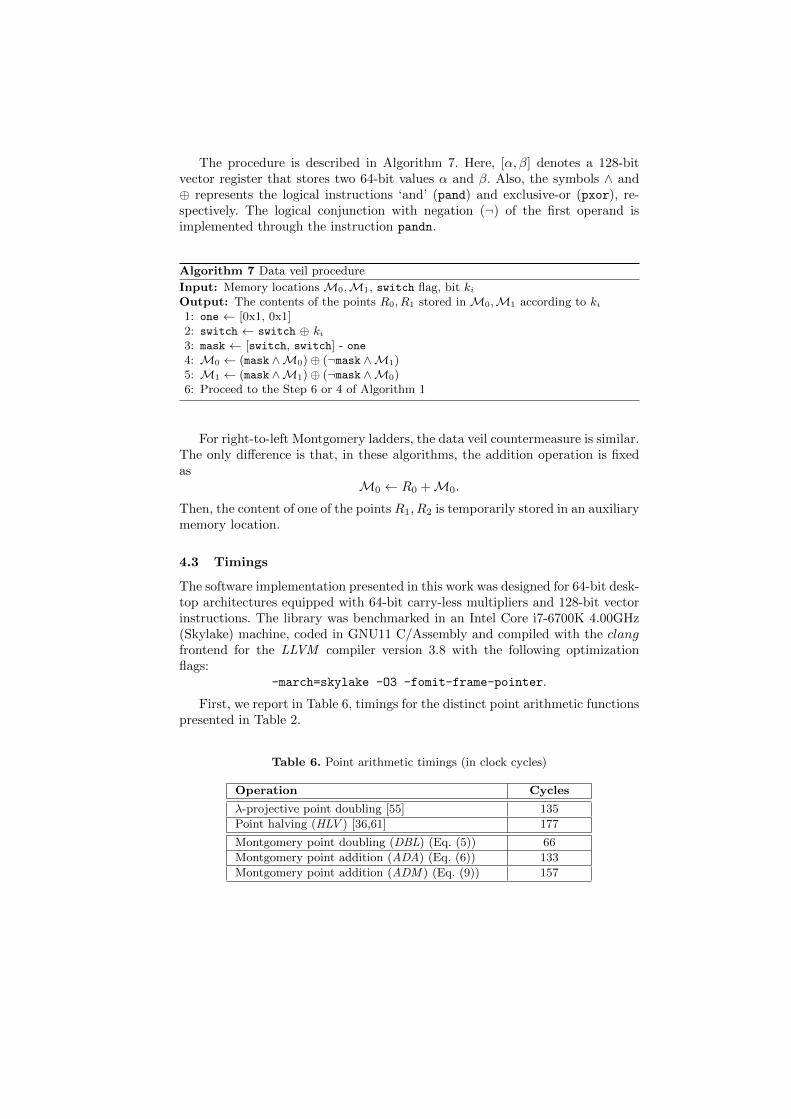
4.3 Timings

The software implementation presented in this work was designed for 64-bit desk-top architectures equipped with 64-bit carry-less multipliers and 128-bit vectorinstructions. The library was benchmarked in an Intel Core i7-6700K 4.00GHz(Skylake) machine, coded in GNU11 C/Assembly and compiled with the clangfrontend for the LLVM compiler version 3.8 with the following optimizationflags:

-march=skylake -O3 -fomit-frame-pointer.

First, we report in Table 6, timings for the distinct point arithmetic functionspresented in Table 2.

Table 6. Point arithmetic timings (in clock cycles)

Operation Cycles

λ-projective point doubling [55] 135

Point halving (HLV ) [36,61] 177

Montgomery point doubling (DBL) (Eq. (5)) 66

Montgomery point addition (ADA) (Eq. (6)) 133

Montgomery point addition (ADM ) (Eq. (9)) 157

Contrary to the estimations presented in Section 3.4, the λ-projective pointdoubling is 23.73% faster than the point halving. One possible explanation isthat, in practice, the latency and throughput of the carry-less multiplier instruc-tion (pclmulqdq) overcomes the cost of multiple memory access on pre-computedtables, inherent in the half-trace (hft) computation. This observation could alsoexplain the fact that the point halving operation is about 2.68 times as costlyas the computation of one Montgomery point doubling.

Also, the extra field multiplication in the ADM addition, when compared tothe ADA corresponds to only 24 clock cycles, which amounts to an extra costof 15.29%.

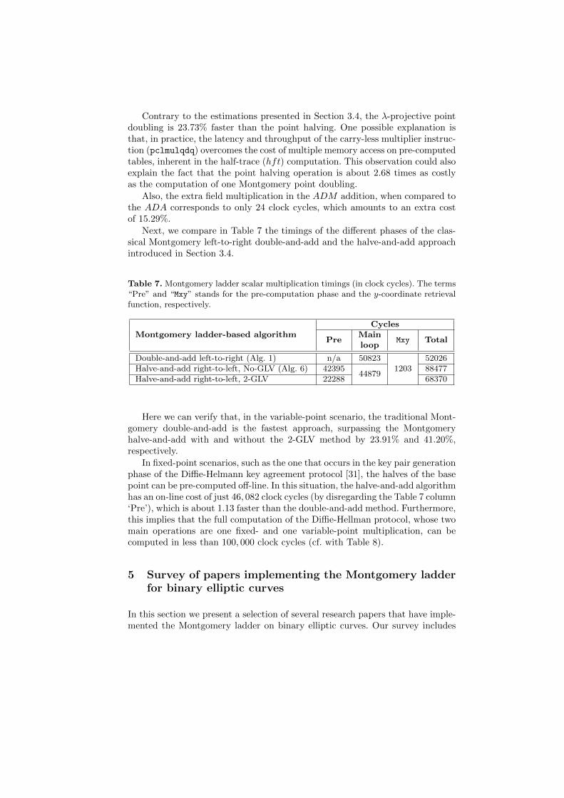
Next, we compare in Table 7 the timings of the different phases of the clas-sical Montgomery left-to-right double-and-add and the halve-and-add approachintroduced in Section 3.4.

Table 7. Montgomery ladder scalar multiplication timings (in clock cycles). The terms“Pre” and “Mxy” stands for the pre-computation phase and the y-coordinate retrievalfunction, respectively.

Montgomery ladder-based algorithmCycles

PreMain

Mxy Totalloop

Double-and-add left-to-right (Alg. 1) n/a 508231203

52026Halve-and-add right-to-left, No-GLV (Alg. 6) 42395

4487988477

Halve-and-add right-to-left, 2-GLV 22288 68370

Here we can verify that, in the variable-point scenario, the traditional Mont-gomery double-and-add is the fastest approach, surpassing the Montgomeryhalve-and-add with and without the 2-GLV method by 23.91% and 41.20%,respectively.

In fixed-point scenarios, such as the one that occurs in the key pair generationphase of the Diffie-Helmann key agreement protocol [31], the halves of the basepoint can be pre-computed off-line. In this situation, the halve-and-add algorithmhas an on-line cost of just 46, 082 clock cycles (by disregarding the Table 7 column‘Pre’), which is about 1.13 faster than the double-and-add method. Furthermore,this implies that the full computation of the Diffie-Hellman protocol, whose twomain operations are one fixed- and one variable-point multiplication, can becomputed in less than 100, 000 clock cycles (cf. with Table 8).

5 Survey of papers implementing the Montgomery ladderfor binary elliptic curves

In this section we present a selection of several research papers that have imple-mented the Montgomery ladder on binary elliptic curves. Our survey includes

both hardware and software implementations that presented a number of re-search novelties in the ladder computation with respect to efficiency and/orside-channel protections.

5.1 The Montgomery ladder on Binary Edwards curves

Let d1, d2 ∈ Fq, such that d1 6= 0 and d2 6= d21 + d1. The Edwards form of abinary elliptic curve is defined as 15

E : d1(x+ y) + d2(x2 + y2) = xy + xy(x+ y) + x2y2. (10)

In such curves, an affine point can be represented using w-coordinates byusing the mapping (x, y) → (w), where w = x + y. However, in order to min-imize the field multiplicative inversion operations, the most efficient formulasfor Edward curves are defined using a mixed coordinate point representationwhere an extra coordinate Z, is defined so that (x, y) → (w) → (W,Z), wherew = x+ y = W

Z .

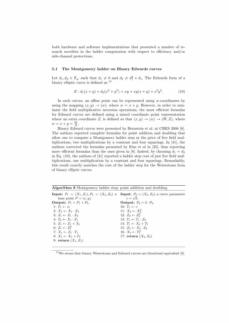
Binary Edward curves were presented by Bernstein et al. at CHES 2008 [8].The authors reported complete formulas for point addition and doubling thatallow one to compute a Montgomery ladder step at the price of five field mul-tiplications, two multiplications by a constant and four squarings. In [41], theauthors corrected the formulas presented by Kim et al in [35], thus reportingmore efficient formulas than the ones given in [8]. Indeed, by choosing d1 = d2in Eq. (10), the authors of [41] reported a ladder step cost of just five field mul-tiplications, one multiplication by a constant and four squarings. Remarkably,this result exactly matches the cost of the ladder step for the Weierstrass formof binary elliptic curves.

Algorithm 8 Montgomery ladder step: point addition and doubling

Input: P1 = (X1, Z1), P2 = (X2, Z2) abase point P = (x, y).

Output: P1 = P1 + P2.1: T1 ← x;2: X1 ← X1 · Z2

3: Z1 ← Z1 ·X2

4: T2 ← X1 · Z1

5: Z1 ← Z1 +X1

6: Z1 ← Z21

7: X1 ← Z1 · T1

8: X1 ← X1 + T2

9: return (X1, Z1)

Input: P2 = (X2, Z2) a curve parameterc =√b.

Output: P2 = 2 · P2.10: T1 ← c11: X2 ← X2

2

12: Z2 ← Z22

13: T1 ← T1 · Z2

14: T1 ← X2 + T1

15: Z2 ← X2 · Z2

16: X2 ← T 21

17: return (X2, Z2)

15We stress that binary Weierstrass and Edward curves are birational equivalent [8].

5.2 Common-Z trick

As shown in Algorithm 8, in a conventional implementation of the Montgomeryladder one requires seven registers (x,X1, Z1, X2, Z2, T1, T2) to compute a ladderstep. However, when dealing with light hardware implementations that must bedeployed over constrained and highly constrained environments, registers cantake up to 80% of the gate area [43]. So, there is a compelling reason for reducingthe number of registers and simplify the register file management.

In [48], Meloni proposed formulas for the common-Z projective coordinatesystem. His formulas were derived in the context of elliptic curves defined overprime fields. Soon after, Lee et al. presented in [43] an adaptation of this idea tothe context of binary elliptic curves, which is based in the following observation.

Two different points P1 = (X1, Z1), P2 = (X2, Z2), can be forced to have thesame Z coordinate by applying the following trick

X1 ← X1 · Z2; (11)

X2 ← X2 · Z1;

Z ← Z1 · Z2.

By assuming that the points P1 and P2 share the same Z coordinate, one hasthat the original Montgomery formulation for point addition (cf. Eq. (6))

ZADD = (X1 · Z2 +X2 · Z1)2;

XADD = x · ZADD +X1 · Z2 ·X2 · Z1;

becomes

ZADD = (X1 +X2)2;

XADD = x · ZADD +X1 ·X2;

whenever Z1 = Z2. Now, since at each ladder step a point doubling must becomputed, one needs to re-apply Eq. (11) to assure that the point that has justbeen doubled (either P1 or P2), still shares the same Z coordinate with the otherpoint (either P2 or P1).

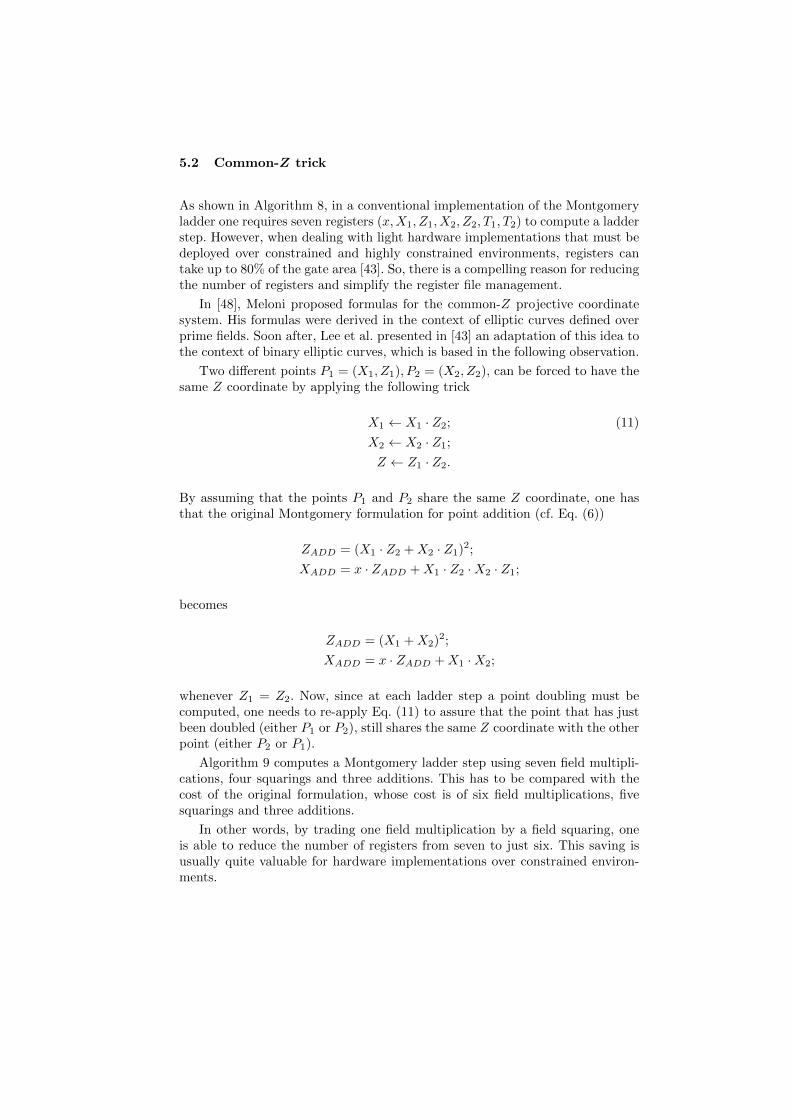
Algorithm 9 computes a Montgomery ladder step using seven field multipli-cations, four squarings and three additions. This has to be compared with thecost of the original formulation, whose cost is of six field multiplications, fivesquarings and three additions.

In other words, by trading one field multiplication by a field squaring, oneis able to reduce the number of registers from seven to just six. This saving isusually quite valuable for hardware implementations over constrained environ-ments.

Algorithm 9 Common-Z point addition and doubling trick [43]

Input: P1 = (X1, Z), P2 = (X2, Z) abase point P = (x, y). A curve param-eter c =

√b.

Output: P1 = P1 + P2, P2 = 2 · P2.1: T2 ← X1 +X2

2: T2 ← T 22

3: T1 ← X1 ·X2

4: X1 ← x5: X1 ← T2 ·X1

6: X1 ← X1 + T1

7: X2 ← X22

8: Z ← Z2

9: T1 ← c10: T1 ← Z · T1

11: Z ← Z ·X2

12: X2 ← X2 + T1

13: X2 ← X22

14: X1 ← X1 · Z15: X2 ← X2 · T2

16: Z ← Z · T2

17: return (X1, Z), (X2, Z)

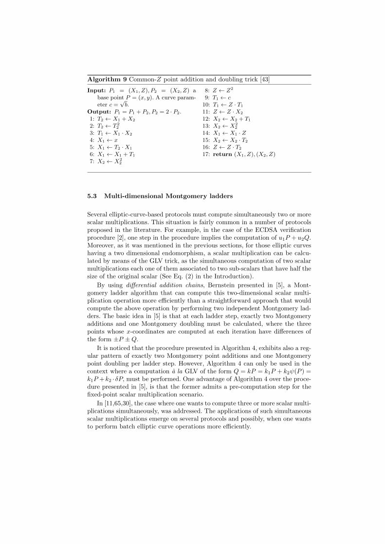
5.3 Multi-dimensional Montgomery ladders

Several elliptic-curve-based protocols must compute simultaneously two or morescalar multiplications. This situation is fairly common in a number of protocolsproposed in the literature. For example, in the case of the ECDSA verificationprocedure [2], one step in the procedure implies the computation of u1P + u2Q.Moreover, as it was mentioned in the previous sections, for those elliptic curveshaving a two dimensional endomorphism, a scalar multiplication can be calcu-lated by means of the GLV trick, as the simultaneous computation of two scalarmultiplications each one of them associated to two sub-scalars that have half thesize of the original scalar (See Eq. (2) in the Introduction).

By using differential addition chains, Bernstein presented in [5], a Mont-gomery ladder algorithm that can compute this two-dimensional scalar multi-plication operation more efficiently than a straightforward approach that wouldcompute the above operation by performing two independent Montgomery lad-ders. The basic idea in [5] is that at each ladder step, exactly two Montgomeryadditions and one Montgomery doubling must be calculated, where the threepoints whose x-coordinates are computed at each iteration have differences ofthe form ±P ±Q.

It is noticed that the procedure presented in Algorithm 4, exhibits also a reg-ular pattern of exactly two Montgomery point additions and one Montgomerypoint doubling per ladder step. However, Algorithm 4 can only be used in thecontext where a computation a la GLV of the form Q = kP = k1P + k2ψ(P ) =k1P +k2 · δP, must be performed. One advantage of Algorithm 4 over the proce-dure presented in [5], is that the former admits a pre-computation step for thefixed-point scalar multiplication scenario.

In [11,65,30], the case where one wants to compute three or more scalar multi-plications simultaneously, was addressed. The applications of such simultaneousscalar multiplications emerge on several protocols and possibly, when one wantsto perform batch elliptic curve operations more efficiently.

5.4 Side channel attacks on Montgomery ladders

Due to its regular pattern execution and the absence of dummy operations,Montgomery ladders are inherently protected against several side-channel at-tacks both in software and hardware implementations. In the case of softwareimplementations, the interested reader is referred to [6,9] and the discussiongiven in this work in §4.2 for protective algorithmic countermeasures.

In the case of hardware implementations, adversaries have much more roomfor launching attacks that in some cases might be devastating [34,17,18]. In [18],the authors reported a careful analysis of the known side-channel attacks andcountermeasures for elliptic curve implementations on hardware platforms. As ithappens, it is often true that a given countermeasure against one specific attackmight make the design vulnerable to other kinds of attacks. In [17], Karaklajicet al. discuss a number of fault attacks against Montgomery ladder hardware im-plementations. The authors also state that the computation of the Montgomeryladder without y-coordinate retrieval can actually protect a hardware implemen-tation against several attacks, such as safe error and sign change attacks.

5.5 Fast and compact Montgomery ladder hardwareimplementations

Montgomery ladders over binary elliptic curves is a favorite choice for hard-ware designers. The main reasons of this lie in the advantage of providing basicprotection against Simple Power Analysis (SPA) [18], the high efficiency of theMontgomery ladder step, namely, only five multiplications and four squaringsare required, and a total of seven registers are needed if the Lopez-Dahab algo-rithm [46] is implemented in a conventional way.

Finally, for many protocols, such as the elliptic curve Diffie-Hellman protocol,the y-coordinate recovering is not necessary, and the absence of the y coordinatecomputation can provide further protection against certain fault attacks.

Among the fastest and most compact hardware accelerators that use theMontgomery ladder on binary elliptic curves, we can mention [45,59] and [41,43],respectively.

Fast Designs In [59], the authors presented a hardware accelerator that com-putes scalar multiplications on binary elliptic curves defined over F2233 thathardly offers a security level of 112 bits. Their design can compute a scalar mul-tiplication in 12.5µS. In [45], the authors targeted NIST standardized binarycurves defined over the fields F2163 , F2233 , and F2283 . For the latter field thepipelined architecture presented in [45] achieved a latency of less than 11µS.

In [58], the authors present a design that manipulates the clock signal sothat their design can operate at its maximum frequency at different steps of theMontgomery ladder point multiplication. This design achieves a performance of

just 6.84µS for a scalar multiplication computed over a binary elliptic curve de-fined over the field F2233 .

In [4], Ay et al. report a hardware accelerator that computes a constant-timevariable-base point multiplication over a GLS elliptic curve that lies in the fieldF22·127 . The prime order subgroup of this curve offers a security level of about127 bits. The authors report a timing delay of just 3.98µS for computing onescalar multiplication on an Xilinx Kintex-7 FPGA device running at 253 MHz.

Compact Designs The authors of [43] reported a hardware architecture thatcan compute a scalar multiplication on Edwards curves defined over the fieldsF2163 ,F2233 and F2283 . The area and time performance reported by the authorsrank among the most efficient hardware accelerators for constrained environ-ments. The authors in [41] adopted the aforementioned common-Z trick to re-duce the number of registers required to carry out one Montgomery ladder step.

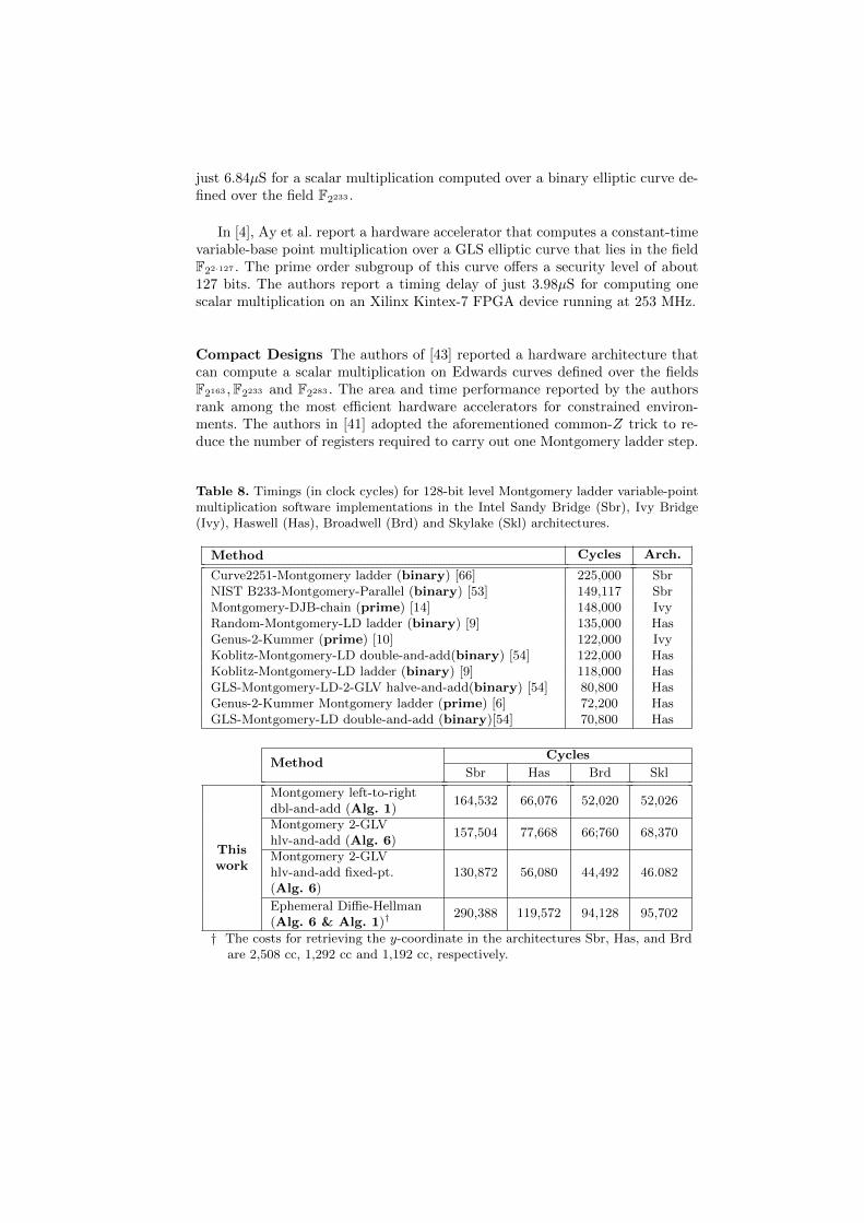
Table 8. Timings (in clock cycles) for 128-bit level Montgomery ladder variable-pointmultiplication software implementations in the Intel Sandy Bridge (Sbr), Ivy Bridge(Ivy), Haswell (Has), Broadwell (Brd) and Skylake (Skl) architectures.

Method Cycles Arch.

Curve2251-Montgomery ladder (binary) [66] 225,000 SbrNIST B233-Montgomery-Parallel (binary) [53] 149,117 SbrMontgomery-DJB-chain (prime) [14] 148,000 IvyRandom-Montgomery-LD ladder (binary) [9] 135,000 HasGenus-2-Kummer (prime) [10] 122,000 IvyKoblitz-Montgomery-LD double-and-add(binary) [54] 122,000 HasKoblitz-Montgomery-LD ladder (binary) [9] 118,000 HasGLS-Montgomery-LD-2-GLV halve-and-add(binary) [54] 80,800 HasGenus-2-Kummer Montgomery ladder (prime) [6] 72,200 HasGLS-Montgomery-LD double-and-add (binary)[54] 70,800 Has

MethodCycles

Sbr Has Brd Skl

Thiswork

Montgomery left-to-rightdbl-and-add (Alg. 1)

164,532 66,076 52,020 52,026

Montgomery 2-GLVhlv-and-add (Alg. 6)

157,504 77,668 66;760 68,370

Montgomery 2-GLVhlv-and-add fixed-pt.(Alg. 6)

130,872 56,080 44,492 46.082

Ephemeral Diffie-Hellman(Alg. 6 & Alg. 1)†

290,388 119,572 94,128 95,702

† The costs for retrieving the y-coordinate in the architectures Sbr, Has, and Brdare 2,508 cc, 1,292 cc and 1,192 cc, respectively.

5.6 Fast Montgomery ladder software implementations

Table 8 presents the performance timings of some of the fastest Montgomeryladders recently reported in the open literature. For the sake of a broader per-spective, several Montgomery ladders operating over prime fields have been in-cluded in this comparison. Notice also that this comparison cannot be quite fair,since the software libraries included in Table 8 were implemented in differentIntel processors, with different capabilities.

Taking into account this consideration, we decided to measure timings of ourcode in various machines that represent the architectures in which the recentworks on Montgomery ladders were implemented: Intel Core i7-2600K 3.40GHz(Sandy Bridge), Intel Core i7-4700MQ 2.40GHz (Haswell) and Intel Core i5-5200U 2.20GHz (Broadwell).

The Intel Skylake software implementation described in this work achievesthe fastest Montgomery ladder performance for a constant-time scalar multi-plication at the 128-bit security level. Furthermore, from the timings reportedin Table 7, it can be seen that the execution of the ephemeral Diffie-Hellmanprotocol can be computed by our software in just 95,702 clock cycles.16

At last, the second part of Table 8 shows that the timings for the SandyBridge are significantly above the ones in the other architectures. For instance,the cost for computing the Montgomery double-and-add is 3.16 times higherwhen compared to the Skylake architecture. The main point here is that, com-pared to the other architectures, the cost of the carry-less multiplication in-struction in the Sandy Bridge machines is more than twice [32]. As a result, toachieve optimal timings in this architecture, the field arithmetic functions haveto be properly designed with alternative instructions.

6 Conclusion

Since the publication in 1987 of the Montgomery ladder procedure, there hasbeen an ever increasing number of research works devoted to analyze and presentalgorithmic improvements to Peter Montgomery’s original idea.

In this survey paper we have striven to present a panoramic review of themain algorithmic ingredients associated to Montgomery ladders and their appli-cations to the fast, side-channel secure and constant-time implementation of thebinary elliptic curve scalar multiplication.

16As the Diffie-Hellman protocol does not need the y coordinate of any point, they-coordinate retrieval function was not considered in this estimation.

Addendum: How to (pre-)compute a ladder on binarycurves

In Sections 3 and 4 we presented the advantages of using the right-to-left Mont-gomery ladder within the fixed-point scenario. The efficiency gain of this right-to-left approach comes from two features. The first, and most essencial, is the mem-ory/speed trade-off in the point doubling operation. The second one is the opti-mization of the point addition formula. That is, given that the points Pi = 2iPcan be pre-computed, we can calculate their affine representation for free andtherefore, save one field multiplication per ladder iteration.

In this section, we focus on the second aspect. More specifically, we showthat the improved point addition formulas for prime curves discussed in [57] canalso be applied for the binary case and, will consequently improve the resultspresented in this document.

Let µ0 =√b/x0 and µ1 = 1/x0. Then the point addition R3 = R0 +R1, with

R2 = R0 −R1, can be written as

A = µ0 · Z1

B = µ1 ·X1

X3 = Z2 · (X1 +A)2

Z3 = X2 · (Z1 +B)2

(12)

which costs four field multiplications, two squarings and two additions. The maindrawback of this formula is the requirement of storing one extra field elementper ladder iteration. Thus, the total storage requirement is of 2mn bits. Notethat the point (0,

√b) has order 2. Such point is not used as a group generator

point in cryptographic applications.

6.1 Koblitz curves

Neal Koblitz proposed in 1991 [38] a family of binary elliptic curves of thefollowing form

E : y2 + xy = x3 + ax2 + 1, (13)

with a ∈ {0, 1}. Such family of curves is famously known for allowing the useof the Frobenius endomorphism to efficiently compute the scalar multiplication.In this work, however, we are interested in its property of having the curveparameter b = 1. In this case, the point addition formula is given as

A = X0 ·X1

B = X0 · Z1

X3 = Z2 · (Z1 +A)2

Z3 = X2 · (X1 +B)2

(14)

having a cost of four field multiplications, two squaring and two additions. Now,assume µ = 1/(x0 + 1). Then Eq. (14) can be written as

A = µ · (X1 + Z1)

X3 = Z2 · (X1 +A)2

Z3 = X2 · (Z1 +A)2(15)

which requires only three field multiplications, two squarings and three additions.

References

1. Agnew, G.B., Mullin R. C., Vanstone S. A.: An Implementation of Elliptic CurveCryptosystems Over F2155 . IEEE Journal on Selected Areas in Communications11(5): 804–813 (1993)

2. ANSI X9.62:2005. Public Key Cryptography for the Financial Services Industry:The Elliptic Curve Digital Signature Algorithm (ECDSA). American NationalStandards Institute (2005)

3. Aranha, D.F., Lopez, J., Hankerson, D.: Efficient Software Implementation of Bi-nary Field Arithmetic Using Vector Instruction Sets. In: Abdalla, M., Barreto,P.S.L.M. (eds.) LATINCRYPT 2010, LNCS, vol. 6212, pp. 144–161. Springer(2010)

4. Ay, A. U., Ozturk, E., Rodrıguez-Henrıquez, F., Savas E.: Design and implementa-tion of a constant-time FPGA accelerator for fast elliptic curve cryptography. In:Athanas, P. M., Cumplido, R., Feregrino C., Sass R. (eds.): International Confer-ence on ReConFigurable Computing and FPGAs, ReConFig 2016 pp. 1–8, IEEE2016.

5. Bernstein, D.J.: Differential Addition Chains. http://cr.yp.to/ecdh/diffchain-20060219.pdf. Accessed Mar 2017.

6. Bernstein, D. J., Chuengsatiansup, C., Lange, T., Schwabe, P.: Kummer StrikesBack: New DH Speed Records. In: Sarkar, P., Iwata, T. (eds.) ASIACRYPT 2014,LNCS, vol. 8873, pp. 317–337. Springer (2014)

7. Bernstein, D. J., Engels, S., Lange, T., Niederhagen, R., Paar, C., Schwabe, P., Zim-mermann. R.: Faster discrete logarithms on FPGAs. Cryptology ePrint Archive,Report 2016/382, 2016. http://eprint.iacr.org/2016/382.

8. Bernstein, D.J., Lange, T., Farashahi, R.: Binary Edwards Curves. In: Oswald, E.,Rohatgi, P. (eds.) CHES 2008, LNCS, vol. 5154, pp. 244–265. Springer (2008)

9. Bluhm, M., Gueron, S.: Fast software implementation of binary elliptic curve cryp-tography. J. Cryptographic Engineering 5(3), 215–226 (2015)

10. Bos, J.W., Costello, C., Hisil, H., Lauter, K.E.: Fast Cryptography in Genus 2.In: Johansson, T., Nguyen, P.Q. (eds.) EUROCRYPT 2013, LNCS, vol. 7881, pp.194–210. Springer (2013)

11. Brown, D.R.L.: Multi-Dimensional Montgomery Ladders for Elliptic Curves.IACR Cryptology ePrint Archive, Report 2006/220. Available at http://

eprint.iacr.org/2006/220 (2006)

12. Chen, B., Hu, C., Zhao, C-A.: A Note on Scalar Multiplication Using DivisionPolynomials. IACR Cryptology ePrint Archive, Report 2015/284. Available athttp://eprint.iacr.org/2015/284 (2015)

13. Chung, P.N., Costello, C., Smith, B.: Fast, uniform, and compact scalar multi-plication for elliptic curves and genus 2 Jacobians with applications to signatureschemes. CoRR abs/1510.03174 (2015)

14. Costello, C., Hisil, H., Smith, B.: Faster Compact Diffie-Hellman: Endomorphismson the x-line. In: Nguyen, P.Q., Oswald, E. (eds.) EUROCRYPT 2014, LNCS, vol.8441, pp. 183–200. Springer (2014)

15. Costello, C., Smith, B.: Montgomery curves and their arithmetic: The case of largecharacteristic fields. IACR Cryptology ePrint Archive, Report 2017/212. Availableat http://eprint.iacr.org/2017/212 (2017)

16. Enge. A., Gaudry, P.: A general framework for subexponential discrete logarithmalgorithms. Acta Arithmetica, 102:83103, 2002.

17. Fan, J., Guo, X., De Mulder, E., Schaumont, P., Preneel, B., Verbauwhede, I.:State-of-the-art of Secure ECC Implementations: A Survey on Known Side-channelAttacks and Countermeasures. IEEE International Symposium on Hardware-Oriented Security and Trust (HOST 2010), pp. 76–87. IEEE (2010)

18. Fan, J., Verbauwhede, I.: An Updated Survey on Secure ECC Implementations:Attacks, Countermeasures and Cost. In: Naccache, D. (eds.) Cryptography andSecurity:, LNCS, vol. 6805, pp. 265–282. Springer (2012)

19. Faugere, J. Perret, L., Petit, C., Renault G.: Improving the Complexity of IndexCalculus Algorithms in Elliptic Curves over Binary Fields. In EUROCRYPT 2012,LNCS, vol. 7237, pages 2744. Springer, 2012.

20. Fong, K., Hankerson, D., Lopez, J., Menezes, A.: Field inversion and point halvingrevisited. IEEE Trans. Comput. 53(8), 1047–1059 (2004)

21. Galbraith, S. D., Gaudry, P.: Recent progress on the elliptic curve discrete loga-rithm problem. Des. Codes Cryptography 78(1): 51-72 (2016)

22. Galbraith, S. D., Lin, X., Scott, M.: Endomorphisms for Faster Elliptic CurveCryptography on a Large Class of Curves. J. Cryptol. 24, 446–469 (2011)

23. Galbraith, S. D., Gebregiyorgis, S. W.: Summation polynomial algorithms for el-liptic curves in characteristic two. In INDOCRYPT 2014, LNCS, vol. 8885, pages409427. Springer, 2014.

24. Galbraith, S. D., Smart, N. P.: A Cryptographic Application of Weil Descent. InCryptography and Coding, LNCS, vol. 1746, pages 191200. Springer, 1999

25. Gallant, R.P., Lambert, R.J., Vanstone, S.A.: Faster Point Multiplication on El-liptic Curves with Efficient Endomorphisms. In: Kilian, J. (ed.) CRYPTO 2001,LNCS, vol. 2139, pp. 190–200. Springer (2001)

26. Gaudry, P., Hess, F., Smart, N. P.: Constructive and destructive facets of Weildescent on elliptic curves. Journal of Cryptology, 15:1946, 2002.

27. Hankerson, D., Karabina, K., Menezes, A.: Analyzing the Galbraith-Lin-ScottPoint Multiplication Method for Elliptic Curves over Binary Fields. IEEE Trans.Comput. 58(10), 1411–1420 (2009)

28. Hess, F.: Generalising the GHS Attack on the Elliptic Curve Discrete LogarithmProblem. LMS Journal of Computation and Mathematics, 7:167192, 2004.

29. Huang, Y.-J., Petit, C., Shinohara, N., Takagi, T.: On Generalized First Fall DegreeAssumptions. IACR Cryptology ePrint Archive 2015: 358 (2015)

30. Hutchinson, A., Karabina, K.: Constructing Multidimensional Differential Addi-tion Chains and their Applications. IACR Cryptology ePrint Archive 2017: 311(2017)

31. Igoe, K., McGrew, D.A., Salter, M.: Fundamental Elliptic Curve CryptographyAlgorithms. RFC 6090, https://rfc-editor.org/rfc/rfc6090.txt. (2015)

32. Intel Corporation: Intel Intrinsics Guide. https://software.intel.com/sites/landingpage/IntrinsicsGuide/. Accessed Mar 2017.

33. Joye, M.: Highly Regular Right-to-Left Algorithms for Scalar Multiplication. InCHES 2007, LNCS, vol. 4727, pp. 135–147. Springer (2007)

34. Karaklajic, D., Fan, J., Schmidt, J-M., Verbauwhede, I.: Low-cost fault detectionmethod for ECC using Montgomery powering ladder. Design, Automation and Testin Europe, DATE 2011 pp. 1016–1021. IEEE (2011)

35. Kim, K.H., lee, C.O., Negre, C.: Binary Edwards Curves Revisited. In: Meier,W., Mukhopadhyay, D. (eds.) INDOCRYPT 2014, LNCS, vol. 8885, pp. 393–408.Springer (2014)

36. Knudsen, E.: Elliptic Scalar Multiplication Using Point Halving. In: Lam, K.Y.,Okamoto, E., Xing, C. (eds.) ASIACRYPT 99, LNCS, vol. 1716, pp. 135–149.Springer (1999)

37. Koblitz, N.: Constructing Elliptic Curve Cryptosystems in Characteristic 2. In:Menezes, A., Vanstone, S. (eds.) CRYPTO 90, LNCS, vol. 537, pp. 156–167.Springer (1991)

38. Koblitz, N.: CM-Curves with Good Cryptographic Properties. In: CRYPTO 91,LNCS, vol. 576, pp. 279–287. Springer (1991)

39. Kocher, P. C.: Timing Attacks on Implementations of Diffie-Hellman, RSA, DSS,and Other Systems. In CRYPTO 96, LNCS, vol. 1109, pp. 104–113. Springer (1996)

40. Koher, D.: Endomorphism rings of elliptic curves over finite fields. PhD thesis, Uni-versity of California Berkeley, (1996). http://echidna.maths.usyd.edu.au/kohel/pub/thesis.pdf. Accessed April 2017.

41. Koziel, B., Azarderakhsh, R., Mozaffari Kermani, M.: Low-Resource and FastBinary Edwards Curves Cryptography. In: Biryukov, A., Goyal, V. (eds.) IN-DOCRYPT 2015, LNCS, vol. 9462, pp. 347–369. Springer (2015)

42. Lang, S.: Elliptic Curves Diophantine Analysis. Springer-Verlag New York, Inc.,USA (1978)

43. Lee, Y.K., Sakiyama, K., Batina, L., Verbauwhede I.: Elliptic-Curve-Based SecurityProcessor for RFID. IEEE Trans. Computers 57(11), 1514–1527 (2008)

44. Lenstra Jr., H. W.: Factoring integers with elliptic curves. Annals of Mathematics.126(3): 649–673 (1987)

45. Li, L., Li, S.: High-Performance Pipelined Architecture of Elliptic Curve ScalarMultiplication Over GF(2m). IEEE Trans. VLSI Syst. 24(4), 1223–1232 (2016)

46. Lopez, J., Dahab, R.: Fast multiplication on elliptic curves over GF(2m) withoutprecomputation. In: Koc, C.K., Paar, C. (eds.) CHES 99, LNCS, vol. 1717, pp.316–327. Springer (1999)

47. Maurer, M., Menezes, A., Teske, E.: Analysis of the GHS weil descent attack on theECDLP over characteristic two finite fields of composite degree. In INDOCRYPT2001, LNCS, vol. 2247, pages 195213. Springer, 2001.

48. Meloni, N.: New Point Addition Formulae for ECC Applications. In: Carlet, C.,Sunar, B. (eds.) WAIFI 2007, LNCS, vol. 4547, pp. 189–201. Springer (2007)

49. Menezes A., Vanstone, S. A.: Elliptic Curve Cryptosystems and Their Implemen-tations. J. Cryptology 6(4): 209–224 (1993)

50. Menezes, A., Qu, M: Analysis of the Weil Descent Attack of Gaudry, Hess andSmart. In CT-RSA 2001, volume 2020 of LNCS, pages 308318. Springer, 2001.

51. Miller, V. S.: Use of Elliptic Curves in Cryptography, Advances in Cryptology. In:Williams, H.C. (eds.) CRYPTO 85, LNCS, vol. 218, pp. 417–426. Springer (1986)

52. Montgomery, P. L.: Speeding the pollard and elliptic curve methods of factoriza-tion. Mathematics of Computation 48, pp. 243–264 (1987)

53. Negre, C., Robert, J-M.: New Parallel Approaches for Scalar Multiplication inElliptic Curve over Fields of Small Characteristic. IEEE Trans. Computers 64(10),2875–2890 (2015)

54. Oliveira, T., Aranha, D.F., Lopez-Hernandez, J., Rodrıguez-Henrıquez, F.: FastPoint Multiplication Algorithms for Binary Elliptic Curves with and without Pre-computation. In: Joux, A., Youssef, A. M. (eds.) SAC 2014, LNCS, vol. 8781, pp.324–344. Springer (2014)

55. Oliveira, T., Aranha, D.F., Lopez-Hernandez, J., Rodrıguez-Henrıquez, F.: Two isthe fastest prime: lambda coordinates for binary elliptic curves. J. CryptographicEngineering 4(1), 3–17 (2014)

56. Oliveira, T., Aranha, D.F., Lopez-Hernandez, J., Rodrıguez-Henrıquez, F.: Improv-ing the performance of the GLS254. http://tinyurl.com/CHES16-Rump.

57. Oliveira, T., Lopez-Hernandez, J., Hisil, H., Rodrıguez-Henrıquez, F.: How to (pre-)compute a ladder. IACR Cryptology ePrint Archive, Report 2017/264. Availableat http://eprint.iacr.org/2017/264 (2017)

58. Rashidi, B., Sayedi, S.M., Farashahi, R.R.: High-speed hardware architecture ofscalar multiplication for binary elliptic curve cryptosystems. Microelectronics Jour-nal 52, 49–65 (2016)

59. Rebeiro, C., Sinha Roy, S., Mukhopadhyay, D.: Pushing the Limits of High-SpeedGF(2m) Elliptic Curve Scalar Multiplication on FPGAs. In: Prouff, E., Schaumont,P. (eds.) CHES 2012, LNCS, vol. 7428, pp. 494–511. Springer (2012)

60. Renes, J., Schwabe, P., Smith, B., Batina, L.: µ Kummer: Efficient HyperellipticSignatures and Key Exchange on Microcontrollers. In: Gierlichs, B., Poschmann,A. Y. (eds.) CHES 2016, LNCS, vol. 9813, pp. 301–320. Springer (2016)

61. Schroeppel, R.: Elliptic curve point halving wins big (2000), In: 2nd Midwest Arith-metical Geometry in Cryptography Workshop.

62. Schroeppel, R.: Automatically solving equations in finite fields (2002), U.S. patent2002/0055962 A1

63. Semaev, I.: Summation polynomials and the discrete logarithm problemon elliptic curves. Cryptology ePrint Archive, Report 2004/031, 2004.http://eprint.iacr.org/2004/031.

64. Semaev, I: New algorithm for the discrete logarithm problem on el-liptic curves. Cryptology ePrint Archive, Report 2015/310, 2015.http://eprint.iacr.org/2015/310.

65. Subramanya Rao, S.R.: Three Dimensional Montgomery Ladder, Differential PointTripling on Montgomery Curves and Point Quintupling on Weierstrass’ and Ed-wards Curves. In: Pointcheval, D., Nitaj, A., Rachidi T. (eds.) AFRICACRYPT2016, LNCS, vol. 9645, pp. 84–106. Springer (2016)

66. Taverne, J., Faz-Hernandez, A., Aranha, D.F., Rodrıguez-Henrıquez, F., Hanker-son, D., Lopez, J.: Speeding scalar multiplication over binary elliptic curves usingthe new carry-less multiplication instruction. J. Cryptographic Engineering 1(3),187–199 (2011)

67. Wenger E., Wolfger, P: Harder, better, faster, stronger: elliptic curve discrete loga-rithm computations on FPGAs. J. Cryptographic Engineering, 6(4):287297, 2016.

Documents

The Montgomery ladder on binary elliptic curves