The Meaning of Structure in InterconnectedDynamic Systems

E. Yeung‡, J. Goncalves∗, H. Sandberg◦, S. Warnick†

Abstract—Interconnected dynamic systems are a pervasivecomponent of our modern infrastructures. The complexity ofsuch systems can be staggering, which motivates simplifiedrepresentations for their manipulation and analysis. This workintroduces the complete computational structure of a system asa common baseline for comparing different simplified represen-tations. Linear systems are then used as a vehicle for comparingand contrasting distinct partial structure representations. Suchrepresentations simplify the description of a system’s completecomputational structure at various levels of fidelity while re-taining a full description of the system’s input-output dynamicbehavior. Relationships between these various partial structurerepresentations are detailed, and the landscape of new realization,minimality, and model reduction problems introduced by theserepresentations is briefly surveyed.

I. INTRODUCTION

Structure and dynamic behavior are two of the most fun-damental concepts characterizing a system. The interplaybetween these concepts has been a central theme in controlas far back as Black’s, Bode’s, or Nyquist’s work on feedbackamplifiers [1], [2], [3], or even as early as Maxwell’s analysisOn Governors in 1868 [4].

The key property driving such analyses is the fact thatan interconnection of systems yields another system. Thisproperty suggests a natural notion of structure, as the inter-connection of systems, and focuses attention on understandinghow interconnections of different systems result in varieties ofdynamic behaviors.

This idea of structure as interconnection is not only criticalin the analysis of systems, but it also plays a key role in systemmodeling. While black box approaches to modeling seek toduplicate the input-output behavior of a system irrespectiveof structure, first principles approaches to modeling use thevisible interconnection structure of a system to decomposethe system into smaller, fundamental components. Constitutiverelations describing each of these components are then applied,and interconnection principles linking these relations thenresult in a model structurally and dynamically consistent withthe original system.

While such approaches have demonstrated remarkable suc-cess in electrical and mechanical domains where systemcomponents are readily visible and physically separated from

For correspondence, please contact eyeung@caltech.edu orsean.warnick@gmail.com. ‡ Control and Dynamical Systems,California Institute of Technology; † Information and Decision AlgorithmsLaboratories, Brigham Young University, Provo, UT; ∗ Control Group,Department of Engineering, University of Cambridge, Cambridge, UK;◦ Automatic Control Laboratory, KTH School of Electrical Engineering,Stockholm, SE.

each other [5], [6], [7], application of such methods to bi-ological, social, and other domains has been more difficult.One reason may be that these systems do not exhibit a naturalstructure in the same sense that previous applications have;while components of electrical and mechanical systems arecompartmentalized and solid-state, the physical relationshipamong components of these other systems are often muchmore fluid [8], [9]. Perhaps for these other domains differentnotions of structure play the role historically occupied by theinterconnection of components.

This paper explores these ideas by characterizing the com-plete computational structure of a system and then contrastingit with three distinct partial structure representations. Thesedifferent representations include the interconnection of sub-systems and the standard idea of a transfer function matrix,but it also includes a newer concept of system structure calledsignal structure that appears to be especially useful for charac-terizing systems that are difficult to compartmentalize. Preciserelationships between these various perspectives of systemstructure are then provided, along with a brief discussion ontheir implications for various questions about realization andapproximation.

II. COMPLETE COMPUTATIONAL STRUCTURE

The complete computational structure of a system char-acterizes the actual processes it uses to sense properties ofits environment, represent and store variables internally, andaffect change externally. At the core of these processes areinformation retrieval issues such as the encoding, storage,and decoding of quantities that drive the system’s dynamics.Different mechanisms for handling these quantities result indifferent system structures.

Mathematically, state equations, or their generalization asdescriptor systems [10], [11], [12] are typically used todescribe these mechanisms. Although there may be manyrealizations that describe the same input-output properties of aparticular system, its complete computational structure is thearchitecture of the particular realization fundamentally usedto store state variables in memory and transform system inputsto the corresponding outputs. In this work we will focus ourattention on a class of differential algebraic systems that areequivalent to a set of ordinary differential equations in statespace form; we will refer to such equations as generalizedstate equations.

Representing a system’s complete computational structureis thus a question of graphically representing the structureimplied by the equations that govern its state evolution. In

arX

iv:1

108.

2755

v1 [

cs.S

Y]

13

Aug

201

1

this work, rather than focusing on the specific syntax of anyone particular graphical modeling language, we will draw fromthe standard system theoretic notions of a block diagram anda signal flow graph to conduct a concrete analysis betweengraphical representations of a system at various levels ofabstraction. The complete computational structure of a system,then, is the description of the system with the most refinedresolution, which we will characterize as a graph derived froma particular block diagram of the generalized state equations.

To make this concept of structure precise, we begin byconsidering a system G with generalized state space realization

x = f (x,w,u),w = g(x,w,u),y = h(x,w,u).

(1)

Note that this system is in the form of a differential algebraicequation, although we will only consider systems with differ-entiation index zero, implying that (1) is always equivalentto a standard ordinary differential or difference equation ofthe same order [13]. Typically we may consider the system(1) to be defined over continuous time, with t ∈ R ≥ 0, andwith u ∈ Rm, x ∈ Rn, w ∈ Rl , y ∈ Rp, and x taken to meandx/dt. Moreover, we restrict our attention to those functionsf , g and h where solutions exist for t ≥ 0. Nevertheless, wecould also consider discrete time systems, with t = 0,1,2,3, ...and x in (1) taken to mean x[t + 1], or systems with generalinput, state, auxiliary, and output spaces U , X , W , or Y ,respectively. In some situations these “spaces” may merelybe sets, e.g. X = {0,1}. In any case, however, we will takeu ∈U m, x ∈X n, w ∈W l , and y ∈ Y p so that m, n, l and pcharacterize the dimensions of the input, state, auxiliary andoutput vectors, respectively.

Note that the auxiliary variables, w, are used to characterizeintermediate computation in the composition of functions.Thus, for example, we distinguish between f (x) = x andf (x) = 2(.5x) by computing the latter as f (w) = 2w andw = g(x) = .5x. In this way, the auxiliary variables serve toidentify stages in the computation of the state space realization(1). Frequently we may not require any auxiliary variables inour description of the system; indeed it is the standard practice[14] to eliminate auxiliary variables to simplify the statedescriptions of systems. Nevertheless, as we discuss structure,it will be critical to use auxiliary variables to distinguishbetween systems with dynamically equivalent, yet structurallydistinct architectures, leading to the following definition.

Definition 1: Given a system (1), we call the number ofauxiliary variables, l, the intricacy of the realization.

To understand the structure of (1), we need a notion ofdependence of a function on its arguments. For example, thefunction f (x,y,z) = xy− x + z clearly depends on z, but itonly depends on x when y 6= 1 (or on y when x 6= 0). Since“structure” refers at some level to the dependence of thesystem variables on each other, it is important that our notionof dependence be made clear.

Definition 2: A function f (w), from l-dimensional domainW to s-dimensional co-domain Z , is said to depend on the

ith variable, wi, if there exist values of the other s−1 variablesw j, j 6= i, such that f (w) is not constant over all values of wiwhile holding the others variables fixed. If s = 1, then f (w)depends on w if it is not constant over all values of w.

Note that when ∂ f/∂wi is well defined, the above definitioncoincides with the partial derivative being non-zero for somevalue of the variables w j. Nevertheless, here we allow fornon-differentiable functions as we explicitly characterize onenotion of the structure of a state space realization.

Definition 3: Given a system G with realization (1), itscomplete or computational structure is a weighted directedgraph C with vertex set V (C ), and edge set E(C ). The vertexset contains m+ n+ l + p elements, with one for each input,state, auxiliary, and output variable of the system; we label thevertices accordingly. In particular, the vertex associated withthe ith input is labeled ui, 1 ≤ i ≤ m, the vertex associatedwith the jth state is labeled f j, 0≤ j≤ n, the vertex associatedwith the kth auxiliary variable is labeled gk, 0≤ k≤ l, and thevertex associated with the rth output is labeled hr, 1≤ r ≤ p.The edge set contains an edge from node i to node j if thefunction associated with the label of node j depends on thevariable produced by node i. Moreover, the edge (i, j) is thenlabeled (weighted) with the variable produced by node i.

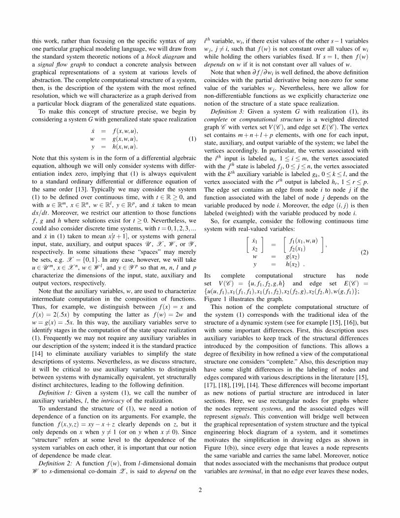
So, for example, consider the following continuous timesystem with real-valued variables:[

x1x2

]=

[f1(x1,w,u)f2(x1)

],

w = g(x2)y = h(x2) .

(2)

Its complete computational structure has nodeset V (C ) = {u, f1, f2,g,h} and edge set E(C ) ={u(u, f1),x1( f1, f1),x1( f1, f2),x2( f2,g),x2( f2,h),w(g, f1)};Figure 1 illustrates the graph.

This notion of the complete computational structure ofthe system (1) corresponds with the traditional idea of thestructure of a dynamic system (see for example [15], [16]), butwith some important differences. First, this description usesauxiliary variables to keep track of the structural differencesintroduced by the composition of functions. This allows adegree of flexibility in how refined a view of the computationalstructure one considers “complete.” Also, this description mayhave some slight differences in the labeling of nodes andedges compared with various descriptions in the literature [15],[17], [18], [19], [14]. These differences will become importantas new notions of partial structure are introduced in latersections. Here, we use rectangular nodes for graphs wherethe nodes represent systems, and the associated edges willrepresent signals. This convention will bridge well betweenthe graphical representation of system structure and the typicalengineering block diagram of a system, and it sometimesmotivates the simplification in drawing edges as shown inFigure 1(b)), since every edge that leaves a node representsthe same variable and carries the same label. Moreover, noticethat nodes associated with the mechanisms that produce outputvariables are terminal, in that no edge ever leaves these nodes,

2

u f1 f2 h u

x1

x1

x2

x2

g w

(a) The complete computational structure C of the simple examplespecified by equation (2).

u f1 f2 h u x1 x2

g w

(b) A modified representation of the complete computational structure ofthe system specified by equation (2). Since the edges leaving a particularnode will always represent the same variable, they have been combinedto simplify the figure.

Fig. 1. The complete computational structure of the state realization of asystem is a graph demonstrating the dependency among all system variables;edges correspond to variables and nodes represent constitutive mechanismsthat produce each variable. System outputs are understood to leave thecorresponding terminal nodes, and system inputs arrive at the correspondingsource nodes.

while the nodes associated with input variables are sources,in that no edge ever arrives at these nodes. Although it iscommon for engineering diagrams to explicitly draw the edgesassociated with output variables and leave them “dangling,”with no explicit terminal node, or to eliminate the inputnodes and simply depict the input edges–also “dangling,” ourconvention ensures that the diagram corresponds to a welldefined graph, with every edge characterized by an orderedpair of nodes. Note also that state nodes, such as f1 in Figure1, may have self loops, although auxiliary nodes will not,and at times it will be convenient to partition the vertex setinto groups corresponding to the input, state, auxiliary, andoutput mechanisms as V (C ) = {Vu(C ),Vx(C ),Vw(C ),Vy(C )}.Likewise, we may similarly partition the edge set as necessary.

We see, then, that knowing the complete structure C ofa system is equivalent to knowing its state space realiza-tion, along with the composition structure with which thesefunctions are represented, given by ( f ,g,h). We refer to thisstructure as computational because it reveals the dependenciesamong variables in the particular representation, or basis, thatthey are stored in and retrieved from memory. These spe-cific, physical mechanisms that store and retrieve information,identified with Vx(C ), are interconnected with devices thattransform variables, identified with Vw(C ), and with devicesthat interface with the system’s external environment. Thesedevices include sensors, identified with Vu(C ), and actuators,identified with Vy(C ), to implement the particular system

behavior observed by the outside world through the manifestvariables, u and y. Although other technologies very wellmay implement the same observed behavior via a differentcomputational structure and a different representation of thehidden variables, x and w, C describes the structure of theactual system employing existing technologies as capturedthrough a particular state description. In this sense, C isthe complete architecture of the system, and often may beinterpreted as the system’s “physical layer.” Importantly, it isoften this notion of structure, or a very related concept, thatis meant when discussing the “structure” of a system, as thenext example illustrates.

A. Example: Graph Dynamical Systems

As an example, we examine the computational structure of agraph dynamical system (GDS). Graph dynamical systems arefinite alphabet, discrete time systems with dynamics defined interms of the structure of an associated undirected graph. Theyhave been employed in the study of various complex systems[20], [21], including• Dynamical process on networks:

– disease propagation over a social contact graph,– packet flow in cell phone communication,– urban traffic and transportation;

• Computational algorithms:– Gauss-Seidel,– gene annotation based on functional linkage net-

works,– transport computations on irregular grids;

• Computational paradigms related to distributed comput-ing.

Here we observe that the computational structure of the graphdynamical system corresponds naturally with the system’sunderlying graph.

Given an undirected graph G with vertex set V (G ) ={1,2, ...,n}, a GDS associates with each node i a state xithat takes its values from a specified finite set X . This stateis then assigned a particular update function that updates itsvalue according to the values of states associated with nodesadjacent to node i on G . Notice that this restriction on theupdate function suggests that the update function for state idepends on states consistent with the structure of G , indicatingthat the system’s computational structure C should correspondto the adjacency structure of G .

The distinction is made between a GDS that updates all ofits states simultaneously, called a parallel GDS, and one thatupdates its states in a particular sequence, called a sequentialGDS. The parallel GDS thus becomes an autonomous dynam-ical system, evolving its state according to its update functionfrom some initial condition. The sequential GDS, on the otherhand, can be viewed as a controlled system that receives aparticular permutation of the node set V (G ) as input and thenevolves its states accordingly.

To illustrate, consider the sequential GDS given by G ={1,2,3,4} as indicated in Figure 2. Let U = {1,2,3,4} and

3

1  

2  

4  

3  

(a) Undirected graph G defining the sequential Graph DynamicalSystem (3).

u

f2 f3

h u

x1

x3

x4 x2

f1 f4

(b) Computational structure C of the sequential Graph DynamicalSystem (3).

Fig. 2. Graph Dynamical Systems are finite alphabet discrete time systemswith dynamics defined in terms of the adjacency structure of a specifiedundirected graph. Here we note that the computational structure of the systemreflects the structure of its underlying graph.

X = Y = {0,1}, with update function given by

x1[t +1]x2[t +1]x3[t +1]x4[t +1]

=

f1(x[t],u[t])f2(x[t],u[t])f3(x[t],u[t])f4(x[t],u[t])

y[t] = x4[t]

(3)

where

fi(x,u) ={

xi u 6= i(1+ xi)(1+ xi−1)(1+ xi+1) u = i (4)

and the arithmetic in (4) is taken modulo 2, while that in thesubscript notation is taken modulo 4 (resulting in x5≡ x1, etc.).So, for example, the initial condition x[0] = [0 0 0 0]T withinput sequence u[t] = 1,2,3,4,1,2,3,4, ... would result in the

following periodic trajectory:

x[1] = [1 0 0 0]T

↓x[2] = [1 0 0 0]T

↓x[3] = [1 0 1 0]T

↓x[4] = [1 0 1 0]T

↓x[8] = [0 0 0 1]T

x[12] = [0 1 0 0]T

↓x[16] = [0 0 1 0]T

↓x[20] = [1 0 0 0]T

↓x[24] = [0 1 0 1]T

↓x[28] = [0 0 0 0]T

The computational structure of the system (3) follows im-mediately from the dependency among variables characterizedby equation (4); Figure 2 illustrates C for this system. Noticethat the structure of G is reflected in C , where the undirectededges in G have been replaced by directed edges in bothdirections, and self-loops have appeared where applicable.Moreover, notice that C considers the explicit influence ofthe input sequence on the update computation, and explicitlyidentifies the system output. In this way, we see that thecomputational structure is a reflection of the natural structureof the sequential GDS.

B. Computational Structure of Linear Systems

Linear systems represent an important special case of thosedescribed by (1). They arise naturally as the linearization ofsufficiently smooth nonlinear dynamics near an equilibriumpoint or limit cycle, or as the fundamental dynamics ofsystems engineered to behave linearly under nominal operatingconditions. In either case, knowing the structure of the relevantlinear system is a critical first step to understanding that of theunderlying nonlinear phenomena.

The general state description of a linear system is given by

x = Ax+ Aw+Bu,w = Ax+ Aw+ Bu,y = Cx+Cw+Du,

(5)

where A ∈ Rn×n, A ∈ Rn×l , A ∈ Rl×n, A ∈ Rl×l , B ∈ Rn×m,B ∈ Rl×m, C ∈ Rp×n, C ∈ Rp×l , and D ∈ Rp×m. Note thatI−A is necessarily invertible, ensuring that the differentiabilityindex of the system is zero. Nevertheless, the matrices areotherwise free.

As in the nonlinear case, it should be apparent that theauxiliary variables are superfluous in terms of characterizingthe dynamic behavior of the system; this idea is made precisein the following lemma. Nevertheless, the auxiliary variablesmake a very important difference in terms of characterizingthe system’s complete computational structure, as illustratedby the subsequent example.

Lemma 1: For any system (5) with intricacy l > 0, thereexists a unique minimal intricacy realization (Ao,Bo,Co,Do)with l = 0 such that for every solution (u(t),x(t),w(t),y(t))of (5), (u(t),x(t),y(t)) is a solution of (Ao,Bo,Co,Do).

Proof: The result follows from the invertibility of (I− A).Solving for w and substituting into the equations of x and ythen yields (Ao,Bo,Co,Do).

4

Consider, for example, the system (5) with state matricesgiven by D = 0 and the following:

A =

[0 00 0

]A =

[0 0 1 0 1 0 1 00 0 0 1 0 1 0 1

]

A =

c1 00 c20 00 00 00 0a1 00 a2

A =

0 0 0 0 0 0 0 00 0 0 0 0 0 0 00 e1 0 0 0 0 0 0e2 0 0 0 0 0 0 00 0 0 0 0 0 0 00 0 0 0 0 0 0 00 0 0 0 0 0 0 00 0 0 0 0 0 0 0

B =

[0 00 0

]BT =

[0 0 0 0 b1 0 0 00 0 0 0 0 b2 0 0

]

C =

[0 00 0

]C =

[1 0 0 0 0 0 0 00 1 0 0 0 0 0 0

](6)

This system has the complete computational structure Cshown in Figure 3(a). Here, because each auxiliary variableis defined as the simple product of a coefficient times anothervariable, we label the node corresponding to wi in C with theappropriate coefficient rather than the generic label, gi. Notethat this realization has an intricacy of l = 8.

Suppose, however, that we eliminate the last six auxiliaryvariables, leading to an equivalent realization with intricacyl = 2. The state matrices then become

A =

[a1 00 a2

]A =

[0 e1e2 0

]

A =

[c1 00 c2

]A =

[0 00 0

]

B =

[b1 00 b2

]BT =

[0 00 0

]

C =

[0 00 0

]C =

[1 00 1

](7)

with computational structure C as shown in Figure 3(b).Similarly, we can find an equivalent realization with l = 0given by

Ao =

[a1 e1c2

e2c1 a2

]Bo =

[b1 00 b2

]Co =

[c1 00 c2

](8)

and all other system matrices equal to zero. This realization,(8), is the minimal intricacy realization of both systems (6)and (7), and its complete computational structure C is givenin Figure 3(c). The equivalence between these realizations iseasily verified by substitution.

Comparing the computational structures for different real-izations of the same system, (6), (7), and (8), we note that

u1

1

1

u2

f1

f2

b1

c2

c1

b2

e1

e2

a1

a2

x1

x2 w2

w1

u2

u1 w7

w5 w3

w4

w6

w8

(a) The complete computational structure C of the linear system givenby the state matrices (6) with intricacy l = 8.

u1

1

1

u2

f1

f2 c2

c1 x1

x2 w2

w1

u2

u1

(b) The complete computational structure C of the equivalent linearsystem with intricacy l = 2, specified by the realization (7).

u1

c2

c1

u2

f1

f2 x2

x1

u2

u1

(c) The complete computational structure C of the minimal intricacy(l = 0) realization for both systems above, characterized by (8).

Fig. 3. The complete computational structure of a linear system characterizedby realizations of differing intricacies. Edges within shaded regions representhidden variables, while those outside shaded regions are manifest variables.

the intricacy of auxiliary variables plays a critical role insuppressing or revealing system structure. Moreover, note thatauxiliary variables can change the nature of which variablesare manifest or hidden. In Figure 3 shaded regions indicatewhich variables, represented by edges, are hidden; manifestvariables leave shaded regions while hidden variables are con-tained within them. Note that the minimal intricacy realization

5

has no internal manifest variables, or, in other words, it hasa single block of hidden variables (Figure 3(c)). Meanwhile,both w1 and w2 are manifest in the other realizations (Figures3(a), 3(b)) since w1 = y1 and w2 = y2, indicated by the “1” attheir respective terminal nodes. This yields two distinct blocksof hidden variables, in either case, revealing the role intricacyof a realization can play characterizing its structure.

The complete computational structure of a system is thusa graphical representation of the dependency among input,state, auxiliary, and output variables that is in direct, one-to-one correspondence with the system’s state realization,generalized to explicitly account for composition intricacy. Allstructural and behavioral information is fully represented bythis description of a system. Nevertheless, this representationof the system can also be unwieldy for large systems withintricate structure.

III. PARTIAL STRUCTURE REPRESENTATIONS

Complex systems are often characterized by intricate com-putational structure and complicated dynamic behavior. Statedescriptions and their corresponding complete computationalstructures accurately capture both the system’s structural anddynamic complexity, nevertheless these descriptions them-selves can be too complicated to convey an efficient under-standing of the nature of the system. Simplified representationsare then desirable.

One way to simplify the representation of a system is torestrict the structural information of the representation whilemaintaining a complete description of the system’s dynamics.The most extreme example of this type of simplified represen-tation is the transfer function of a single-input single-outputlinear time invariant (LTI) system. A transfer function com-pletely specifies the system’s input-output dynamics withoutretaining any information about the computational structure ofthe system. For example, consider the nth order LTI single-input single-output system given by (A,b,c,d). It is wellknown that although the state description of the system com-pletely specifies the transfer function, G(s) = c(sI−A)−1b+d,the transfer function G(s) has an infinite variety of staterealizations, and hence computational structures, that all char-acterize the same input-output behavior. That is, the structuralinformation in any state realization of the system is completelyremoved in the transfer function representation of the system,even though the dynamic (or behavioral) information aboutthe system is preserved.

We use this power of a transfer function to obfuscatestructural information to develop three distinct partial-structurerepresentations of an LTI system: subsystem structure, signalstructure, and the sparsity pattern of a (multiple input, multipleoutput) system’s transfer function matrix. Later we will showhow each of these representations contain different kinds ofstructural information, and we will precisely characterize therelationships among them.

A. Subsystem Structure

One of the most natural ways to reduce the structural infor-mation in a system’s representation is to partition the nodesof its computational structure into subsystems, then replacethese subsystems with their associated transfer function. Eachtransfer function obfuscates the structure of its associatedsubsystem, and the remaining (partial) structural informationin the system is the interconnection between transfer functions.

Subsystem structure refers to the appropriate decompositionof a system into constituent subsystems and the interconnec-tion structure between these subsystems. Abstractly, it is thecondensation graph of the complete computational structuregraph, C , taken with respect to a particular partition of Cthat identifies subsystems in the system. Such abstractionshave been used in various ways to simplify the structuraldescriptions of complex systems [15], [22], for example by“condensing” strongly connected components or other groupsof vertices of a graph into single nodes. Nevertheless, inthis work we define a particular condensation graph as thesubsystem structure of the system. We begin by characterizingthe partitions of C that identify subsystems.

Definition 4: Given a system G with realization (5) and as-sociated computational structure C , we say a partition of V (C )is admissible if every edge in E(C ) between components ofthe partition represents a variable that is manifest, not hidden.

For example, considering the system (8) withV (C ) = {u1, f1,c1,c2, f2,u2}. We see that the partition{(u1),( f1,c1,c2, f2),(u2)} is admissible since the only edgesbetween components are u1(u1, f1) and u2(u2, f2), representingthe manifest variables u1 and u2. Notice that the shadingin Figure 3(c) is consistent with this admissible partition.Alternatively, the partition {(u1),( f1,c1),(c2, f2),(u2)} is notadmissible for (8), since the edges x1( f1, f2) and x2( f2, f1)extend between components of the partition but representvariables x1 and x2 that are hidden, not manifest.

Although sometimes any aggregation, or set of fundamentalcomputational mechanisms represented by vertices in C , maybe considered a valid subsystem, in this work a subsystemhas a specific meaning. In particular, the variables that inter-connect subsystems must be manifest, and thus subsystemsare identified by the components of admissible partitions ofV (C ). We adopt this convention to 1) enable the distinctionbetween real subsystems vs. merely arbitrary aggregations ofthe components of a system, and 2) ensure that the actualsubsystem architecture of a particular system is adequately re-flected in the system’s computational structure and associatedrealization, thereby ensuring that such realization is complete.

Definition 5: Given a system G with realization (5) andassociated computational structure C , the system’s subsystemstructure is a condensation graph S of C with vertex setV (S ) and edge set E(S ) given by:

• V (S ) = {S1, ...Sq} are the elements of an admissiblepartition of V (C ) of maximal cardinality, and

• E(S ) has an edge (Si,S j) if E(C ) has an edge fromsome component of Si to some component of S j.

6

We label the nodes of V (S ) with the transfer function of theassociated subsystem, which we also denote Si, and the edgesof E(S ) with the associated variable from E(C ).

Note that, like C , the subsystem structure S is a graph withvertices that represent systems and edges that represent signals,or system variables. For example, Figure 4(a) illustrates thesubsystem structure for both systems (6) and (7), shown inFigures 3(a) and 3(b). Note that the subsystem structure ofthese systems’ minimally intricate realization, (8), is quitedifferent, with a single block rather than two blocks intercon-nected in feedback, as shown in Figure 4(b). This illustratesthe necessity of auxiliary variables to adequately describe thecomplete system structure.

u1 S1 1 u1 w1

u2 S2

w2 1 u2

(a) The subsystem structure S of the linear system given by the statematrices (6) with intricacy l = 8. Note that the subsystem structure of theequivalent, but less intricate system given by equation (7) is exactly thesame, indicated by the shaded regions in Figures 3(a) and 3(b).

u1 S u2 u1 u2

(b) The subsystem partial structure S of the dynamically equivalent,minimally intricate linear system, specified by the realization (8) cor-responding to Figure 3(c).

Fig. 4. The subsystem structure of a linear system partitions vertices ofthe complete computational structure and condenses admissible groups ofnodes into single subsystem nodes, shown in brown; nodes shown in greenare those that correspond directly to unaggregated vertices of the completecomputational structure, which will always be associated with mechanismsthat generate manifest variables. Here, the subsystem structure corresponds tothe interconnection of shaded regions in Figure 3. Comparing Figures 4(a) and4(b), we note that intricacy in a realization may be necessary to characterizemeaningful subsystems and yield nontrivial subsystem structure.

Lemma 2: The subsystem structure S of a system G, withcomplete computational structure C , is unique.

Proof: We prove by contradiction. Suppose the subsystemstructure S of G is not unique. Then there are at least twodistinct subsystem structures of G, which we will label S 1 andS 2. This implies there are two admissible partitions of V (C ),given by V (S 1) and V (S 2), such that V (S 1) 6=V (S 2) andwith equal cardinality, q. Note that by definition, q must bethe maximal cardinality of any admisible partition of V (C ).To obtain a contradiction, we will construct another admissiblepartition, V (S 3), such that |V (S 3)|> q.

Consider the following partition of V (C ) that is a refinement

of both V (S 1) and V (S 2):

V (S 3) = {S3|S3 6= /0;S3 = Si∩S j,Si ∈V (S 1),S j ∈V (S 2)}.

Since V (S 1) 6= V (S 2), then |V (S 3)| > q, since the cardi-nality of the refinement must then be greater than that ofV (S 1) or V (S 2). Moreover, note that the partition V (S 3) isadmissible, since every edge of C between vertices associatedwith distinct components of V (S 3) corresponds with an edgeof either S 1 or S 2, which are admissible. Thus, V (S 3) isan admissible partition of V (C ) with cardinality greater thanq, which contradicts the assumption that S 1 and S 2 are bothsubsystem structures of G.

The subsystem structure of a system reveals the way naturalsubsystems are interconnected, and it can be represented inother ways besides (but equivalent to) specifying S . Forexample, one common way to identify this kind of subsystemarchitecture is to write the system as the linear fractionaltransformation (LFT) with a block diagonal “subsystem” com-ponent and a static “interconnection” component (see [23]for background on the LFT). For example, the system inFigure 4(a) can be equivalently represented by the feedbackinterconnection of a static system N : U×W→ Y× (U×W)and a block-diagonal dynamic system S : U×W→W givenby

N =

0 0 1 00 0 0 11 0 0 00 0 0 10 0 1 00 1 0 0

, S =

[S1 00 S2

], (9)

where

S1 :[

u1w2

]→ w1 S2 :

[w1u2

]→ w2 (10)

In general, the LFT associated with S will have the form

N =

[0 IL K

]S =

S1 0 ...

0. . .

... 0 Sq

(11)

where q is the number of distinct subsystems, and L and K areeach binary matrices of the appropriate dimension (see Figure5). Note that if additional output variables are present, besidesthe manifest variables used to interconnect subsystems, thenthe structure of N and S above extend naturally. In any event,however, N is static and L and K are binary matrices.

The subsystem structure of any system is well definedalthough it may be trivial (a single internal block) if thesystem does not decompose naturally into an interconnectionof subsystems, such as (8) in Figure 3(c) and Figure 4(b).Note that S always identifies the most refined subsystemstructure possible, and for systems with many interconnectedsubsystems, coarser representations may be obtained by ag-gregating various subsystems together and constructing theresulting condensation graph. These coarser representationseffectively absorb some interconnection variables and their

7

€

S1 0 0 0 Sq

⎡

⎣

⎢ ⎢ ⎢

⎤

⎦

⎥ ⎥ ⎥

€

0 IL K⎡

⎣ ⎢

⎤

⎦ ⎥

u y

w π(u,w)

Fig. 5. The subsystem structure of a system can always be represented by thelower linear fractional transformation of the static interconnection matrix Nwith a block diagonal transfer function matrix S. Note that π(u,w) representsa permutation of a subset of the variables in the vector inputs, u, and manifestauxiliary variables, w, possibly with repetition of some variables if necessary.

associated edges into the aggregated components, suggestingthat such representations are the subsystem structure for lessintricate realizations of the system, where some of the manifestauxiliary variables are removed, or at least left hidden. Thesubsystem structure is thus a natural partial description ofsystem structure when the system can be decomposed intothe interconnection of specific subsystems.

B. Signal Structure

Another very natural way to partially describe the structureof a system is to characterize the direct causal dependenceamong each of its manifest variables; we will refer to thisnotion as the signal structure. This description of the structureof a system makes no attempt to cluster, or partition, the actualinternal system states. As a result, it offers no informationabout the internal interconnection of subsystems, and signalstructure can therefore be a very different description of systemstructure than subsystem structure.

Given a generalized linear system (5) with complete com-putational structure C , we characterize its signal structure byconsidering its minimal intricacy realization (Ao,Bo,Co,Do).We assume without loss of generality that the outputs y areordered in such a way that Co can be partitioned

Co =

[C11 C12C21 C22

]where C11 ∈ Rp1×p1 is invertible, with p1 equal to therank of Co; C12 ∈ Rp1×(n−p1); C21 ∈ R(p−p1)×p1 ; and C22 ∈R(p−p1)×(n−p1). Note that if the outputs of the minimal intri-cacy realization do not result in C11 being invertible, then itis possible to reorder them so the first p1 outputs correspondto independent rows of Co; the states can then be renumberedso that C11 is invertible. One can show that such reorderingof the outputs and states of the minimal intricacy realization

only affects the ordering of the states and outputs of the orig-inal system; the graphical relationship of the computationalstructure is preserved.

The direct causal dependence among manifest variables isthen revealed as follows. First, since Co is rank p1, the rank-nullity theorem guarantees Co has nullity n− p1. Let

Nn−p1 =

[N1N2

],

where N1 ∈ Rp1×(n−p1), N2 ∈ R(n−p1)×(n−p1), be a matrix ofcolumn vectors that form a basis for the null space of Co. Bythe definition of N and the invertibility of C11, we can write

N =

[−C−1

11 C12N2N2

].

Since the columns of N form a basis, we deduce that N2 isinvertible; thus the state transformation z = T x given by

T =

[C11 C120 N−1

2

]. (12)

is well defined. This transformation yields a system of theform [

z1z2

]=

[A11 A12A21 A22

][z1z2

]+

[B1B2

]u

[y1y2

]=

[I 0

C2 0

][z1z2

]+

[D1D2

]u

(13)

where C2 =C21C−111 , z1 ∈ Rp1 , z2 ∈ Rn−p1 , u ∈ Rm, y1 ∈ Rp1 ,

and y2 ∈Rp−p1 . To simplify the exposition we will abuse no-tation and refer to the above system as (A,B,C,D), since thereis little opportunity to confuse these matrices with those of theoriginal system given in (5). In fact, the system (13) is simplya change of coordinates of the minimal intricacy realization(Ao,Bo,Co,Do), possibly with a reordering of the output andstate variables. The direct causal dependence among manifestvariables is then revealed by the dynamical structure functionof (A,B,

[I 0

],D1).

The dynamical structure function of a class of linear systemswas defined in [24] and discussed in [25], [26], [27], [28],[29], [30]. This representation of a linear system describes thedirect causal dependence among a subset of state variables,and it will extend to characterize signal structure for thesystem in (13). We repeat and extend the derivation hereto demonstrate its applicability to the system (13). TakingLaplace transforms and assuming zero initial conditions yieldsthe following relationships[

sZ1sZ2

]=

[A11 A12A21 A22

][Z1Z2

]+

[B1B2

]U (14)

where Z(s) denotes the Laplace transform of z(t), etc. Solvingfor Z2 in the second equation and substituting into the first thenyields

sZ1 =W (s)Z1 +V (s)U (15)

8

where W (s) =[A11 +A12(sI−A22)

−1A21]

and V (s) =[B1 +A12(sI−A22)

−1B2]. Let D(s) be the matrix of the di-

agonal entries of W (s), yielding

Z1 = Q(s)Z1 +P(s)U (16)

where Q(s) = (sI− D(s))−1(W (s)− D(s)) and P(s) = (sI−D(s))−1V (s). From (13) we note that Z1 = Y1−D1U , which,substituting into (16), then yields:[

Y1Y2

]=

[Q(s)C2

]Y1 +

[P(s)+(I−Q(s))D1

D2

]U (17)

We refer to the matrices[Q(s)T CT

2]T [

(P(s)+(I−Q(s))D1)T DT

2]T

as Q and P, respectively. The matrices (Q(s),P(s)) are calledthe dynamical structure function of the system (13), and theycharacterize the dependency graph among manifest variablesas indicated in Equation (17). We note a few characteristicsof (Q(s),P(s)) that give them the interpretation of systemstructure, namely:• Q(s) is a square matrix of strictly proper real rational

functions of the Laplace variable, s, with zeros on thediagonal. Thus, if each entry of y1 were the node of agraph, Qi j(s) would represent the weight of a directededge from node j to node i; the fact Qi j(s) is properpreserves the meaning of the directed edge as a causaldependency of yi on y j.

• Similarly, the entries of the matrix [P(s)+(I−Q(s))D1]are proper and thus carry the interpretation of causalweights characterizing the dependency of entries of y1on the m inputs, u. Note that when D1 = 0, this matrixreduces to P(s), which has strictly proper entries.

This leads naturally to the definition of signal structure.Definition 6: The signal structure of a system G, with

realization (5) and equivalent realization (13), and with dy-namical structure function (Q(s),P(s)) characterized by (16),is a directed graph W , with a vertex set V (W ) and edge setE(W ) given by:• V (W ) = {u1, ...,um,y11, ...,y1p1 ,y21, ...,y2p2}, each repre-

senting a manifest signal of the system, and• E(W ) has an edge from ui to y1 j, ui to y2 j, y1i to y1 j or

y1i to y2 j if the associated entry in [P(s)+(I−Q(s))D1],D2, Q(s), or C21 (as given in Equations (16) and (17)) isnonzero, respectively.

We label the nodes of V (W ) with the name of the associatedvariable, and the edges of E(W ) with the associated transferfunction entry from Equation (17).

Signal structure is fundamentally a different type of graphthan either the computational or subsystem structure of asystem because, unlike these other graphs, vertices of asystem’s signal structure represent signals rather than systems.Likewise, the edges of W represent systems instead of signals,as opposed to C or S . We highlight these differences byusing circular nodes in W , in contrast to the square nodesin C or S . The next example illustrates a system without

notable subsystem structure and no apparent structural motifin its complete computational structure; nevertheless, it revealsa simple and elegant ring structure in its signal structure.

Example 1: Ring Signal Structure. Systems with no ap-parent structure in any other sense can nevertheless possessa very particular signal structure. Consider the minimallyintricate linear system, specified by the state-space realization(Ao,Bo,Co,Do), where

Ao =112

−178 262 −10 −141 −19 88

−156 252 −12 −156 −48 84

−158 266 −38 −147 −5 128

−12 48 −12 −72 −12 12

−288 504 0 −264 −180 144

0 24 0 −24 −12 −12

,

Bo =14

0 −1 210 0 12−8 1 270 0 00 0 00 0 0

,

Co =

−1 4 −1 −2 −1 1

−12 21 0 −11 −5 6

0 2 0 −2 −1 0

, Do =

0 0 00 0 00 0 0

.(18)

f1

f2

f3

f6

f5

f4

u2

u1

u3

h2

h1

h3

Fig. 6. The complete computational structure C , of the system(Ao,Bo,Co,Do) given by (18). Here, edge labels, u and x, and self loopson each node fi have been omitted to avoid the resulting visual complexity.Edges associated with variables x, which are not manifest, are entirelycontained within the shaded region (which also corresponds to the strongpartial condensation shown in Figure 7(a)).

We compute the signal structure by employing a changeof coordinates on the state variables to find an equivalent

9

u2 S

u1 u1

u2

u3 u3

(a) The subsystem structure, S , of the system shown in Figures 6 and7(b); the system has no interconnection structure between subsystemsbecause the system is composed of only a single subsystem; it does notmeaningfully decompose into smaller subsystems.

y2

y1 y3

u1 u3

u2

Q21 Q32

Q13

P11

P22

P33

(b) The signal structure, W , of the system shown in Figures 6 and 7(a).Note that, in contrast with C and S , vertices of W represent manifestsignals (characterized by round nodes), while edges represent systems.

Fig. 7. Distinct notions of partial structure for the system (Ao,Bo,Co,Do)given by Equation (18). Observe that while the system is unstructured inthe strong sense, it is actually quite structured in the weak sense. Moreover,although the subsystem structure is visible in the complete computationalstructure (Figure 6) as a natural condensation (note the shaded region), thesignal structure is not readily apparent.

realization of the form (13). The transformation

T =

−1 4 −1 −2 −1 1−12 21 0 −11 −5 6

0 2 0 −2 −1 00 0 0 1 0 00 0 0 0 1 00 0 0 0 0 1

(19)

results in the following realization

A = TA0T−1 =

−2 0 0 0 0 −30 −3 0 −1 0 00 0 −4 0 5 01 0 0 −4 0 00 2 0 0 −5 00 0 1 0 0 −1

B = T B0 =

2 0 00 3 00 0 60 0 00 0 00 0 0

,

C =C0T−1 =[

I3 0],

D = D0 = [0].

(20)The dynamical structure function of the system, (Q,P), thenbecomes

Q =

0 0 −3

s2+3s+2−1

s2+7s+12 0 0

0 10s2+9s+20 0

,

P =

2

s+2 0 0

0 3s+3 0

0 0 6s+4

(21)

which yields the signal structure, W , as shown in Figure 7(b).Notice that although the complete computational structureand subsystem structure do not characterize any meaningfulinterconnection patterns, the system is nevertheless structuredand organized in a very concrete sense. In particular, theoutputs y1, y2, and y3 form a cyclic dependency, and eachcausally depends on a single input ui, i = 1,2,3,, respectively.

C. Sparsity Structure of the Transfer Function Matrix

The weakest notion of structure exhibited by a system is thepattern of zeros portrayed in its transfer function matrix, where“zero” refers to the value of the particular transfer functionelement, not a transmission zero of the system. Like signalstructure, this type of structure is particularly meaningfulfor multiple-input multiple-output systems, and, like signalstructure, the corresponding graphical representation reflectsthe dependance of system output variables on system inputvariables. Thus, nodes of the graph will be signals, representedby circular nodes, and the edges of the graph will representsystems, labeled with the corresponding transfer functionelement; a zero element thus corresponds to the absence ofan edge between the associated system input and output.Formally, we have the following definition.

Definition 7: The sparsity structure of a system G is adirected graph Z , with a vertex set V (Z ) and edge set E(Z )given by:• V (Z ) = {u1, ...,um,y1, ...,yp}, each representing a mani-

fest signal of the system, and

10

• E(Z ) has an edge from ui to y j if G ji is nonzero.We label the nodes of V (Z ) with the name of the associatedvariable, and the edges of E(Z ) with the associated elementfrom the transfer function G(s).

Unlike signal structure, note that the sparsity structure of thetransfer function matrix describes the closed-loop dependencyof an output variable on a particular input variable, not itsdirect dependence. As a result, the graph is necessarily bipar-tite, and all edges will begin at an input node and terminate atan output node; no edges will illustrate dependencies betweenoutput variables. For example, the sparsity structure for thesystem in Example 1, is shown in Figure 8, with transferfunction G(s) =

n1(s)d(s)

−90(s+4)d(s)

−18(s3+12s2+47s+60)d(s)

−2(s3+10s2+29s+20)d(s)

3(s5+16s4+97s3+274s2+352s+160)d(s)

18(s+5)d(s)

−20(s+1)d(s)

30(s3+7s2+14s+8)d(s)

n2(s)d(s)

, (22)

where d(s) = s6 + 19s5 + 145s4 + 565s3 + 1174s2 + 1216s +450, n1(s) = 2(s5 + 17s4 + 111s3 + 343s2 + 488s+ 240), andn2(s) = 6(s5 + 15s4 + 85s3 + 225s2 + 274s + 120). Although

y2

y1

y3

u1

u3

u2

G11

G33

G22

G12

G32

G31

G13

G21

G23

Fig. 8. The sparsity structure for the system in Example 1. Note that verticesof sparsity structure are manifest signals, distinguished in this work by circularnodes similar to those of signal structure. Nevertheless, this system has a fullyconnected (and thus unstructured) sparsity structure, while its signal structure(shown in Figure 7(b)) exhibits a definite ring structure.

the direct dependence, given by the signal structure, is cyclic(Figure 7(b)), there is a path from every input to every outputthat does not cancel. Thus, the sparsity structure is fullyconnected, corresponding to the full transfer function matrixin Equation (22).

It is important to understand that the sparsity structure doesnot necessarily describe the flow of information between inputsand outputs. The presence of a zero in the (i, j)th locationsimply indicates that the input-output response of the systemresults in the ith output having no dependence on the jth input.Such an effect, however, could be the result of certain internal

cancellations and does not suggest, for example, that there isno path in the complete computational structure from the jth

input to the ith output. Thus, for example, a diagonal transferfunction matrix does not imply the system is decoupled.

The next example demonstrates that a fully coupled systemmay, nevertheless, have a diagonal transfer function, evenwhen the system is minimal in both intricacy and order.That is, the internal cancellations necessary to generate thediagonal sparsity structure in the transfer function while beingfully coupled do not result in a loss of controllability orobservability. Thus, the sparsity structure only describes theinput-output dependencies of the system and does not implyanything about the internal information flow or communicationstructure. This fact is especially important in the context ofdecentralized control, where the focus is often on shaping thesparsity of a controller’s transfer function given a particularsparsity in the transfer function of the system to be controlled.

Example 2: Diagonal Transfer Function 6= Decoupled.Consider a system, G, with the following minimal intricacyrealization, (Ao,Bo,Co,Do):[

x1x2

]=

[−5 12 −4

][x1x2

]+

[2 14 −1

][u1u2

][

y1y2

]=

[1 1−4 2

][x1x2

](23)

It is easy to see from (Ao,Bo,Co,Do) that this system has afully connected complete computational structure. Moreover,one can easily check that the realization is controllable and ob-servable, and thus of minimal order. Nevertheless, its transferfunction is diagonal, given by

G(s) =[ 6

s+3 00 −6

s+6

]. (24)

IV. RELATIONSHIPS AMONG REPRESENTATIONS OFSTRUCTURE

In this section, we explore the relationships between the fourrepresentations of structure defined above. What we will findis that some representations of structure are more informativethan others. Next, we will discuss a specific class of systemsin which the four representations of structure can be rankedby information content (with one representation encapsulatingall the information contained in another representation ofstructure). Outside this class of systems, however, we willdemonstrate that signal structure and subsystem structure havefundamental differences in addition to those arising from thegraphical conventions of circular versus square nodes, etc.Signal and subsystem structure provide alternative ways ofdiscussing a system’s structure without requiring the full detailof a state-space realization or the abstraction imposed bya transfer function. Understanding the relationships betweenthese representations then enables the study of new kinds ofresearch problems that deal with the realization, reconstruc-tion, and approximation of system structure (where structurecan refer to the four representations defined so far or other

11

representations of structure not mentioned in this work). Thefinal section gives a discussion of such future research.

Different representations of structure contain different kindsof structural information about the system. For example,the complete computational structure details the structuraldependencies among fundamental units of computation. Usingcomplete computational structure to model system structurerequires knowledge of the parameters associated with eachunit of computation. Partial representations of structure suchas signal and subsystem structure do not require knowledge ofsuch details in their description. Specifically, subsystem struc-ture essentially aggregates units of computation to form sub-systems and models the closed-loop transfer function of eachsubsystem. Signal structure models the SISO transfer functionsdescribing direct causal dependencies between outputs andinputs of some of the fundamental units of computation thathappen to be manifest. Sparsity structure models the closed-loop dependencies of system outputs on inputs. Thus, completecomputational structure appears to be the most demanding orinformation-rich description of system structure. This intuitionis made precise with the following result:

Theorem 1: Suppose a complete computational structurehas minimal intricacy realization (Ao,Bo,Co,Do) with

C0 =

[C11 C12C21 C22

]and C11 invertible. Then the complete computational structurespecifies a unique subsystem, signal, and sparsity structure.

Proof: Let C be a computational structure with minimalintricacy realization (Ao,Bo,Co,Do) with

C0 =

[C11 C12C21 C22

],

C11 invertible. By Lemma 2, the subsystem structure S isunique. Since C11 is invertible, we see that equations (15)and (17) imply that the minimal intricacy realization uniquelyspecifies the dynamical structure function of the system. Bydefinition, the signal structure is unique. Finally, write thegeneralized state-space realization of C as

(A,B,C,D) =

([A AA A

],

[BB

],[

C C],D).

The uniqueness of the sparsity structure follows from itsone-to-one correspondence with the transfer function G(s) =Co(sI−Ao)

−1Bo +Do which can also be expressed as

(C+C(I− A)−1A)(sI−A− A(I− A)−1A)−1(B+ B(I− A)−1A).

It is well known that a transfer function G(s) can be realizedusing an infinite number of state-space realizations. Withoutadditional assumptions, e.g. full state feedback, it is impossibleto uniquely associate a single state-space realization with agiven transfer function. On the other hand, a state spacerealization specifies a unique transfer function. In this sense, atransfer function contains less information than the state spacerealization.

Similarly, subsystem, signal, and sparsity structure can berealized using multiple complete computational structures.Without additional assumptions, it is impossible to associatea unique complete computational structure with a given sub-system, signal, or sparsity structure. Theorem 1 shows that acomplete computational structure specifies a unique subsys-tem, signal, and sparsity structure. In this sense, a completecomputational structure is a more informative description ofsystem structure than subsystem, signal and sparsity structure.The next result has a similar flavor and follows directly fromthe one-to-one correspondence of a system’s transfer functionwith its sparsity structure.

Theorem 2: Every subsystem structure or signal structurespecifies a unique sparsity structure.

Proof: Consider the LFT representation F (N,S) of asubsystem structure S ; write

N =

[0 IL K

]as in equation (11). The linear fractional transform gives theinput-output map, i.e. the transfer function. Thus, G(s) = (I−SK)−1SL.

Similarly, using the dynamical structure representation ofthe signal structure W given in equation (17), we can solvefor the transfer function

G(s) =(

I−[

Q(s) 0C2 0

])−1 [ P(s)+(I−Q(s))D1D2

]The result follows from the definition of sparsity structure.

The relationship between subsystem structure and signalstructure is not so straightforward. Nevertheless, subsystemstructure does specify a unique signal structure for a class ofsystems, namely systems with subsystem structure composedof single output (SO) subsystems and where every manifestvariable is involved in subsystem interconnection. For thisclass of systems, subsystem structure is a richer descriptionof system structure than signal structure.

A. Single Output Subsystem Structure and Signal Structure

Theorem 3: Let S be a SO subsystem structure with LFTrepresentation F (N,S). Suppose

N =

[0 IL K

],

where[L K

]has full column rank. Then S uniquely spec-

ifies the signal structure of the system.Proof: The dynamics of N and S satisfy

Y = [0]U +[I]Y (25)π = LU +KY (26)Y = Sπ (27)

Combining the second and third equation, we get

Y = Sπ = S[K L

][YU

].

12

Since S is a SO subsystem structure, the entries of S describedirect causal dependencies among manifest variables involvedin interconnection. Since

[L K

]has full column rank and

is a binary matrix, this means that each manifest variable isused at least once in interconnection. Thus, S describes thedirect causal dependencies between all manifest variables ofthe system and specifies the signal structure of the system.Notice that for the class of systems described above, the fourrepresentations of structure can be ordered in terms of infor-mation content. Theorem 1 shows that the complete computa-tional structure uniquely specifies all the other representationsof structure and thus is the most informative of the four. ByTheorem 3 and Theorem 2 respectively, subsystem structureuniquely specifies the signal structure and sparsity structure ofthe system and thus is the second most informative. Similarly,signal structure is the third most informative and sparsitystructure is the least informative of the four representationsof structure.

We note that the converse of Theorem is also true, namelyif the subsystem structure of a system specifies a uniquesignal structure then the subsystem structure is a SO subsystemstructure where every manifest variable is an interconnectionvariable. The proof is simple and follows from the resultof the next subsection. We also provide several examplesthat show how a multiple output subsystem structure can beconsistent with multiple signal structures - these all will serveto illustrate the general relationship between subsystem andsignal structure outside of the class of systems mentionedabove.

B. The Relationship Between Subsystem and Signal Structure

Subsystem structure and signal structure are fundamentallydifferent descriptions of system structure. In general, subsys-tem structure does not encapsulate the information containedin signal structure. Signal structure describes direct causaldependencies between manifest variables of the system. Sub-system structure describes closed loop dependencies betweenmanifest variables involved in the interconnection of subsys-tems. Both representations reveal different perspectives of asystem’s structure. The next result makes this relationshipbetween subsystem and signal structure precise.

Theorem 4: Given a system G, let F (N,S) be the LFTrepresentation of a subsystem structure S . In addition, letthe signal structure of the system G be denoted as in equation(17). Let Y (Si) denote the outputs associated with subsystemSi. Define

[Qint(s)]i j ≡

{Qi j(s) yi,y j ∈ Y (Sk),Sk a subsystem in S

0 otherwise,

and Qext ≡ Q(s) − Qint(s). Then the signal structure andsubsystem structure are related in the following way:

S[

L K]= (I−Qint)

−1 [ P Qext]

(28)

Proof: Examining relation (28), observe that the i jth entryof the left hand side describes the closed loop causal depen-dency from the jth entry of

[UT Y T ]T to Yi. By closed

loop, we mean that they do not describe the internal dynamicsof each subsystem, e.g. the direct causal dependencies amongoutputs of a single subsystem. Thus, these closed loop causaldependencies are obtained by solving out the intermediatedirect causal relationships, i.e. the entries in Qint . Notice thatthe right hand side of (28) also describes the closed loop mapfrom

[UT Y T ]T to Y, and in particular the i jth entry of

(I−Qint)−1 [ P Qext

]describes the closed loop causal dependency from the jth entryof[

U Y]T to Yi.

As a special case, notice that for SO subsystem structures,Qint becomes the zero matrix and that for subsystem structureswith a single subsystem, S becomes the system transferfunction, L becomes the identity matrix, Qint = Q, and Qextand K are both zero matrices. The primary import of this resultis that a single subsystem structure can be consistent with twoor more signal structures and that a single signal structure canbe consistent with two or more subsystem structures. Considerthe following examples:

Example 3: A Signal Structure consistent with two Subsys-tem StructuresIn this example, we will show how a signal structure canbe consistent with two subsystem structures. To do this weconstruct two different generalized state-space realizations thatyield the same minimal intricacy realization but differentadmissible partitions (see Definition 4). The result is twodifferent subsystem structures that are associated with the samesignal structure. First, we consider the complete computationalstructure C1 with generalized state-space realization

(A1,B1,C1,D1) =

([A1 A1A1 A1

],

[B1B1

],[

C1 C1],D1

)where

A1 =

−4 1 0 0 11 −7 0 0 30 0 −6 0 00 0 0 −6 01 2 0 0 −10

, A1 =

0 0 2 10 0 2 12 1 0 11 2 2 00 0 0 0

,

A1 =

1 0 0 0 00 1 0 0 00 0 1 0 00 0 0 1 00 0 0 0 0

, A1 = [0]4 ,

B1 =[

1 1 1 1 1]T

, B1 =[

0 0 0 0],

C1 = 04×5, C1 = I4,

and D1 = 04×1. Figure 9(a) shows the computational structureC1.

13

ff2

ff1

x2

x1 x2

ff5

x5

gg2

gg1

11

w4

ff3 gg3

ff4

x3 x4

gg4 11

uu1

w2

11w1

x5 x1

w3

x3

11

u1

u1

u1

u1

w2

u1

w1

w1

w2

w3

w4

w4

w3

x4

x1

x2

(a) The complete computational structure C1 with generalized state-spacerealization (A1,B1,C1,D1). We have omitted the self-loops on each of the fvertices for the sake of visual clarity.

ff2

ff1

x2

x1 x2

ff5

x5

gg2

gg1

11

w4

ff3 gg3

ff4

w4

gg4 11

uu1

w2

11w1

x5 x1

w3

x3

11

u1

u1

u1

u1

w2

u1

w1

w1

w2

w3

w4

w4

w3

x4

x1

x2

(b) The complete computational structure C2 with generalized state-spacerealization (A2,B2,C2,D2). We have omitted the self-loops on each of the fvertices for the sake of visual clarity.

Fig. 9. The complete computational structures of two systems that differ onlyby a slight rearrangement of their state-space dynamics. The rearrangementresults in two different subsystem structure representations. Nonetheless, theresulting minimal intricacy realization for both systems is the same, implyingthat both systems have an identical signal structure.

Next consider the complete computational structure C2 with

generalized state-space realization

(A2,B2,C2,D2) =

([A2 A2A2 A2

],

[B2B2

],[

C2 C2],D2

).

The matrix entries of this generalized state-space realizationare given as follows:

A2 =

−4 1 0 0 11 −7 0 0 30 0 −6 1 00 0 2 −6 01 2 0 0 −10

, A2 =

0 0 2 10 0 2 12 1 0 01 2 0 00 0 0 0

A2 = A1, A2 = [0]4 ,

B2 = B1 = 15×1, B2 = B1 = 04×1,

C2 =C1, C2 = C1,

and D2 = D1. Figure 9(b) shows the computational structureC2. The difference between these two computational structuresis evident more in the subsystem structure representation ofthe system - note how replacing A1 with A2, essentiallyexternalizes internal dynamics. The result is that C2 admits asubsystem structure S2 which divides one of the subsystemsof S1 into two subsystems. This is more apparent in the LFTrepresentations of S1 and S2; the LFT representation of S1is given by F (N1,S1) =

N1 =

04×1 I400100010001

0 0 1 00 0 0 10 0 0 01 0 0 00 1 0 00 0 0 10 0 0 01 0 0 00 1 0 00 0 1 00 0 0 0

and

S1(s) =

S11(s) 0 00 S12(s) 00 0 S13(s)

,with S11(s),S12(s),S13(s) given by

[2(s2+18s+76)

s3+21s+130s+234s2+18s+76

s3+21s+130s+234s2+19s+86

s3+21s2+130s+2342(s2+15s+52)

s3+21s2+130s+234s2+15s+52

s3+21s2+130s+234(13+s)(s+5)

s3+21s2+130s+234

],

[ 2s+6

1s+6

1s+6

1s+6

],[ 1

s+62

s+62

s+61

s+6

]respectively.

14

The LFT representation of S2(s) is represented as the LFTF (N2,S2) = where

N2 =

04×1 I4001001

0 0 1 00 0 0 10 0 0 01 0 0 00 1 0 00 0 0 0

and S2(s),S21(s),S22(s) respectively given as[

S21(s) 00 S22(s)

],[

2(s2+18s+76)s3+21s2+130s+234

s2+18s+76s3+21s2+130s+234

s2+19s+86s3+21s2+130s+234

2(s2+15s+52)s3+21s2+130s+234

s2+15s+52s3+21s2+130s+234

(13+s)(s+5)s3+21s2+130s+234

],

[2s+13

s2+12s+34s+8

s2+12s+347+s

s2+12s+34s+10

s2+12s+342(7+s)

s2+12s+34s+8

s2+12s+34

].

However, if we consider the minimal intricacy realiza-tions of C1,C2 we get the same state-space realization(Ao,Bo,Co,Do) with

Ao =

−4 1 2 1 11 −7 2 1 32 1 −6 1 01 2 2 −6 01 2 0 0 −10

, Bo =

11111

C =

[I4 04×1

]The signal structure of the system is thus specified by thedynamical structure function (Q,P)(s), with

Q(s) =

0 12+s

s2+14s+392(s+10)

s2+14s+39s+10

s2+14s+3913+s

s2+17s+64 0 2(s+10)s2+17s+64

s+10s2+17s+64

2s+6

1s+6 0 1

s+61

s+62

s+62

s+6 0

P(s) =

11+s

s2+14s+3913+s

s2+17s+641

s+61

s+6

Example 4: A Subsystem Structure consistent with two Sig-

nal StructuresNow we consider a subsystem structure with multiple signalstructures. Recalling the discussion above, subsystem structuredescribes the closed loop causal dependencies between man-ifest interconnection variables and signal structure specifiesdirect causal dependencies between manifest variables. Whenit is impossible to determine these direct causal dependenciesby inspection from the closed loop causal dependencies in asubsystem structure representation, then there can be multiplesignal structures that are consistent with the subsystem struc-ture.

Reconsider S2. The LFT is given by F (N2,S2) where

N2 =

04×1 I4001001

0 0 1 00 0 0 10 0 0 01 0 0 00 1 0 00 0 0 0

and

S2 =

[S21 00 S22

],

with S21 and S22 given by

[2(s2+18s+76)

s3+21s2+130s+234s2+18s+76

s3+21s2+130s+234s2+19s+86

s3+21s2+130s+2342(s2+15s+52)

s3+21s2+130s+234s2+15s+52

s3+21s2+130s+234(13+s)(s+5)

s3+21s2+130s+234

],

[2s+13

s2+12s+34s+8

s2+12s+347+s

s2+12s+34s+10

s2+12s+342(7+s)

s2+12s+34s+8

s2+12s+34

]

respectively.

If we consider the relation

S2[

K L]= (I−Qint)

−1 [ Qext P],

we can take (Q,P)(s) to equal

Q1(s) =

0 12+s

s2+14s+392(s+10)

s2+14s+39s+10

s2+14s+3913+s

s2+17s+64 0 2(s+10)s2+17s+64

s+10s2+17s+64

2s+6

1s+6 0 1

s+61

s+62

s+62

s+6 0

P1(s) =

11+s

s2+14s+3913+s

s2+17s+641

s+61

s+6

with

Qint ≡

0 12+s

s2+14s+39 0 0

13+ss2+17s+64 0 0 0

0 0 0 1s+6

0 0 2s+6 0

15

and Qext ≡ Q1−Qint , or Q2(s) =

0 0 2(s2+18s+76)s3+21s2+130s+234

s2+18s+76s3+21s2+130s+234

0 0 2(52+15s+s2)s3+21s2+130s+234

52+15s+s2

s3+21s2+130s+234

2s+13s2+12s+34

s+8s2+12s+34 0 0

s+10s2+12s+34

2(7+s)s2+12s+34 0 0

P2(s) =

s2+19s+86s3+21s2+130s+234

(13+s)(s+5)s3+21s2+130s+234

7+ss2+12s+34

s+8s2+12s+34

and taking Qint ≡ [0] and Qext ≡ Q2. It is routine to showthat with these definitions, both (Q1,P1)(s) and (Q2,P2)(s)are consistent with S2. Thus a single subsystem structurecan be consistent with two signal structures. It is importantto note that one of our signal structures exhibited directcausal dependencies corresponding exactly with the closedloop dependencies described by subsystem structure. We notethat this correspondence sometimes occurs (as in the case ofTheorem 3) but generally does not hold.

V. IMPACT ON SYSTEMS THEORY

The introduction of partial structure representations suggestsnew problems in systems theory. These problems explore therelationships between different representations of the samesystem, thereby characterizing properties of the different repre-sentations. For example, classical realization theory considersthe situation where a system is specified by a given transferfunction, and it explores how to construct a consistent statespace description. Many important ideas emerge from theanalysis:

1) State realizations are generally more informative thana transfer function representation of a system, as thereare typically many state realizations consistent with thesame transfer function,

2) Order of the state realization is a sensible measure ofcomplexity of the state representation, and there is awell-defined minimal order of any realization consistentwith a given transfer function; this minimal order isequal to the Smith-McMillian degree of the transferfunction,

3) Ideas of controllability and observability of a staterealization characterize important properties of the real-ization, and any minimal realization is both controllableand observable.

In a similar way, introducing partial structure representationsimpacts a variety of concepts in systems theory, includingrealization, minimality, and model reduction.

A. Realization

The definition of partial structure representations enrichthe kinds of realization questions one may consider. In the

previous section, we demonstrated that partial structure repre-sentations of a system are generally more informative than itstransfer function but less informative than its state realization.Thus, two classes of representation questions emerge: recon-struction problems and structure realization problems (Figure10).

Fig. 10. Partial structure representations introduce new classes of realiza-tion problems: reconstruction and structure realization. These problems aredistinct from identification, and each depends on the type of partial structurerepresentation considered.

Reconstruction problems consider the construction of a par-tial structure representation of a system given its transfer func-tion. Because partial structure representations are generallymore informative than a transfer function, these problems areill-posed–like the classical realization problem. Nevertheless,one may consider algorithms for generating canonical repre-sentations, or one may characterize the additional informationabout a system–beyond knowledge of its transfer function–that one would require in order to specify one of its partialstructure representations. In particular, we may consider twotypes of reconstruction problems:

1) Signal Structure Reconstruction: Given a transferfunction G(s) with its associated sparsity structure Z ,find a signal structure, W , with dynamical structurefunction (Q,P) as in Equation (17) such that G =(I−Q)−1P,

2) Subsystem Structure Reconstruction: Given a transferfunction G(s) with its associated sparsity structure Z ,find a subsystem structure, S , with structured LFT(N,S) as in Equation (11) such that G = (I−SK)−1SL.

Signal structure reconstruction is also called network recon-struction, particularly in systems biology where it plays acentral role. There, the objective is to measure fluctuationsof various proteins, or other chemical species, in response toparticular perturbations of a biochemical system, and then infercausal dependencies among these species [31], [32], [29], [24],[33], [34].

Structure realization problems then consider the construc-tion of a state space model, possibly generalized to includeauxiliary variables as necessary, consistent with a given partialstructure representation of a system. Like the classical realiza-tion problem or reconstruction problems, these problems arealso ill-posed since there are typically many state realizationsof a given partial structure representation of a system. Also,like reconstruction problems, these realization problems canbe categorized in two distinct classes, depending on the type

16

of partial structure representation that is given:3) Signal Structure Realization: Given a system G with

signal structure W and associated dynamical structurefunction (Q,P), find a state space model (A,B,C,D)consistent with (Q,P), i.e. such that Equations (14-17)hold,

4) Subsystem Structure Realization: Given a system Gwith subsystem structure S and associated structured(N,S) (recorded in the LFT representation F (N,S)),find a generalized state space model of the form ofEquation (5) consistent with (N,S).

Signal structure realization may sometimes be called networkrealization, consistent with the nomenclature for signal struc-ture reconstruction.

Note that all the reconstruction and structure realizationproblems here are distinct from identification problems, justas classical realization is different from identification. For thesystems considered here, identification refers to the use ofinput-output data (and no other information about a system)to choose a representation that best describes the data in someappropriate sense. Because input-output data only character-izes the input-output map of a system, identification can atbest characterize the system’s transfer function; no informationabout structure, beyond the sparsity structure, is availablein such data. In spite of this distinction, however, it is notuncommon for reconstruction problems to be called structureidentification problems. Nevertheless, one may expose suchproblems as the concatenation of an identification and areconstruction problem and precisely characterize the extrainformation needed to identify such structure by carefullyanalyzing the relevant reconstruction problem, independent ofthe particular identification technique [24], [31].

B. Minimality

Just as partial structure representations enrich the classicalrealization problem, they also impact the way we think aboutminimality. Certainly the idea of a minimal complexity repre-sentation is relevant for each of the four problems listed above,but clearly the relevant notion of complexity may be differentdepending on the representation. We consider each situationas follows:

1) Minimal Signal Structure Reconstruction: In thissituation one needs to consider how to measure thecomplexity of a system’s signal structure, W , or itsassociated dynamical structure function, (Q,P). Somechoices one may consider could be the number of edgesin W , the maximal order of any element in (Q,P), orthe maximal order of any path from any input ui toany output y j. The problem would then be to find aminimal complexity signal structure consistent with agiven transfer function.

2) Minimal Subsystem Structure Reconstruction: In thissituation one needs to consider how to measure thecomplexity of a system’s subsystem structure, S , orits associated structured LFT, (N,S). One notion could

be to measure complexity by the number of distinctsubsystems; the problem would then be to find theminimal complexity subsystem structure representationconsistent with a given transfer function. Another notioncould be the number of non-zero entries in the S matrix,where (N,S) denote the the LFT associated with thesubsystem structure. Using this measure, a single sub-system block with no zero entries would be considered amore complex representation than a subsystem structurewith a large number of distinct, albeit interconnected,subsystems.

3) Minimal Signal Structure Realization: In this situationone needs to consider how to measure the complexityof a system’s zero-intricacy state realization, from whichsignal structure is derived. The obvious choice would beto use the order of the realization as a natural measureof complexity, and the problem would then be to findthe minimal order state realization [29], [35] consistentwith a given signal structure, W , or, equivalently, withits associated dynamical structure function, (Q,P). Notethat this minimal order is guaranteed to be finite (forthe systems considered here) and can easily be shownto be greater or equal to the Smith-McMillian degreeof the transfer function specified by the signal structure;we call this number the structural degree of the signalstructure [25].

4) Minimal Subsystem Structure Realization: In thissituation one needs to consider how to measure the com-plexity of a generalized state realization in the presenceof auxiliary variables. Both the order and the intricacy ofthe realization offer some perspective of its complexity,but one needs to consider how they each contribute to theoverall complexity of the realization. The problem wouldthen be to find a minimal complexity generalized staterealization consistent with a given subsystem structure.

These various problems demand new ideas for thinkingabout the complexity of a system’s representation, especiallythat of a partial structure representation. These new ideas aboutcomplexity, in turn, introduce opportunities for characterizingminimality of a representation in terms that add insight to ourunderstanding of the relationship between a system’s behaviorand its structure, much as controllability and observabilitycharacterize classical notions of minimality in a system’s staterealization. Besides suggesting the need for a characterizationof minimality, however, these ideas also impact notions ofapproximation and how we think about model reduction.

C. Model Reduction

Each of the reconstruction and structure realization prob-lems described above have associated with them not onlya minimal-representation version of the problem, but alsoan approximate-representation version of the problem. Theminimal-representation versions of these problems, as de-scribed above, seek to construct a representation of minimalcomplexity in the targeted class that is nevertheless consistent

17

with the system description provided. Similarly, approximate-representation versions of these problems seek to construct arepresentation in the targeted class that has a lower complexitythan the minimal complexity necessary to deliver consistencywith the system description provided. As a result, consistencywith the given system description can not be achieved, someasures of approximation become necessary to sensiblydiscuss a “best” representation of the specified complexity.

For example, associated with the classical realization prob-lem is the standard model reduction problem. In this situation,a transfer function is specified, and one would like to constructa state realization with a complexity that is lower than thatwhich is necessary (for such a realization to be consistentwith the given transfer function) that nevertheless “best”approximates it. Note that the appropriate notion of complexitydepends on the target representation class; here, the targetrepresentation class is the set of state realizations, so theappropriate notion of complexity is model order. Likewise,note that the appropriate notion of approximation depends onthe type of system representation that is initially provided;here, a transfer function is provided, so an appropriate measureof approximation could be an induced norm, such as H∞.Thus, one could measure the quality of an approximation bymeasuring the induced norm of the error between the giventransfer function and that specified by the approximate staterealization. Note that since the H∞ model reduction problemremains open, many alternative measures and approaches havebeen suggested [36], [37], [23]. In any event, because thespecified system description is a transfer function, the resultingmeasure of approximation is typically one that either directlyor indirectly measures the difference in input-output dynamicbehavior between the approximate model and the given systemdescription; the focus is on dynamics, not system structure,when considering notions of approximation in the standardmodel reduction problem.

Similarly, there is an appropriate reduction problem asso-ciated with each of the minimal reconstruction and minimalstructure realization problems described above. Like standardmodel reduction, the appropriate notion of complexity ischaracterized by the class of target representations, while theappropriate measure of approximation depends on the systemrepresentation that is initially provided. To make these ideasmore concrete, we discuss each of the problems individually:

1) Approximate Signal Structure Reconstruction: Inthis situation one would like to find a signal structurerepresentation with lower complexity e.g. fewer numberof edges, etc. than the minimal level of complexitynecessary to specify a given transfer function. Whenusing the number of edges as a complexity measure,this problem may be interpreted as trying to restrictthe number of communication links between individualcomputation nodes in a distributed system while approx-imating some desired global dynamic. The appropriatemeasure of approximation, then, is any measure thatsensibly compares the desired transfer function from thatspecified by the reduced signal structure, such as H∞.

2) Approximate Subsystem Structure Reconstruction:In this situation one would like to find a subsystemstructure representation with lower complexity than theminimal level of complexity necessary to specify agiven transfer function. If one considers the numberof subsystems as the measure of complexity, then thisproblem is trivial since any transfer function is consistentwith a subsystem structure with a single subsystem. Ifone measures complexity by the number of non-zeroentries in the S matrix, where (N,S) denote the the LFTassociated with the subsystem structure, then it appearslikely that one could often formulate a meaningfulapproximation problem.

Unlike these approximate reconstruction problems, approx-imate realization problems may have dual relevant measuresof approximation, since having an initial partial structurerepresentation of a system also always specifies its transferfunction. Measuring the similarity between transfer functionsdetermines the degree to which a lower order system approx-imates the dynamics of a given system, while measuring thesimilarity between partial structure representations determinesthe degree to which a lower order system approximates thestructure of a given system.

3) Approximate Signal Structure Realization: In thissituation one would like to find a state realization witha model complexity that is lower than the minimalcomplexity necessary to specify a given signal structure.Typically the complexity of a generalized state realiza-tion would be measured by both the order and intricacyof the realization. Since signal structure only dependson the zero intricacy realization of a system, however,a minimal complexity realization will always have zerointricacy; thus model order is the only relevant notionof complexity. Moreover, since the structural degree ofa particular signal structure may be strictly greater thanthe Smith-McMillian degree of the transfer function itspecifies, a few distinct kinds of approximation problemsemerge: structural approximation and dual approxima-tion (Figure 11).

a) Structural Approximation: When the order of theapproximation is less than the structural degreeof the given signal structure but greater than theSmith-McMillian degree of the associated transferfunction, the resulting approximation can specifythe given transfer function exactly, even though itssignal structure only approximates that of the givensystem. Note that the sense in which similarity insignal structure should be measured is an area ofon-going research.

b) Dual Approximation: When the order of theapproximation is less than the Smith-McMilliandegree of the transfer function specified by thegiven signal structure, then it will represent neitherthe structure nor the dynamics of the given systemexactly.

18

Fig. 11. Approximate signal structure realization leads to two distincttypes of reduction problems. Structural approximation exactly realizes thedynamics of a given signal structure while only approximating its structure;dual approximation captures neither the dynamics nor the structure of a givensignal structure exactly.

4) Approximate Subsystem Structure Realization: Inthis situation one would like to find a generalized staterealization with a model complexity that is lower thanthe minimal complexity necessary to specify a givensubsystem structure. Here, complexity of a generalizedstate realization is measured both in terms of intricacyand order since intricacy of a realization directly impactsthe number of admissible subsystem blocks (see Figure3) while order impacts the ability of the realizationto approximate the transfer function specified by thegiven subsystem structure. As a result, three distinct ap-proximation problems emerge to complement subsystemstructure realization: Structure-Preserving Model Reduc-tion, Subsystem Structure Approximation, SubsystemDual Approximation (Figure 12).

a) Structure-Preserving Model Reduction: Whenthe intricacy of an approximation is high enough,the subsystem structure of a system can be pre-served while its dynamic behavior is approximatedby lower-order systems. A naive approach to suchreduction would be to reduce the order of varioussubsystems. However, even when each subsystemis well approximated, the dynamic behavior ofthe overall interconnection may be very differentfrom the original system. As a result, methodshave been developed in this area for approximating

the dynamics of the closed-loop, interconnectedsystem while preserving its subsystem structure[38], [39], [40].

b) Subsystem Structure Approximation: When theorder of an approximation is high enough, the dy-namic behavior of a system can be preserved whileis subsystem structure is approximated by lower-intricacy realizations. The sense in which similarityof subsystem structure should be measured remainsan open topic for research.

c) Subsystem Dual Approximation: When both theorder and the intricacy of an approximation arelower than the minimal values necessary to realizea given subsystem structure and the transfer func-tion it specifies, then the objective of the reductionproblem is to find the realization of the specifiedcomplexity that best approximates the structure anddynamics of the given system.

Fig. 12. Approximate subsystem structure realization leads to three dis-tinct types of reduction problems: 1) Structure-preserving model reductionpreserves the subsystem structure of a given system while approximatingits dynamic behavior, 2) Subsystem structure approximation preserves thedynamic behavior but approximates the subsystem structure, and 3) Subsystemdual approximation captures neither the structure nor the dynamic behaviorof a system described by a particular subsystem structure.

The introduction of partial structure representations suggestsa number of new problems in systems theory. These problemsinclude new classes of realization problems, called reconstruc-tion and structural realization problems, as well as a numberof new reduction problems. Each of these problems differdepending on the partial structure representation one considers,and a number of research issues remain to properly formulatemost of them. The overview offered here is merely meant togive a perspective of the landscape of problems that emergeswith the introduction of partial structure representations.

VI. CONCLUSION

This paper introduced the idea of a system’s completecomputational structure as a baseline for comparing simplifiedrepresentations. Although closely aligned with a system’s state

19

space realization, we demonstrated the need for auxiliaryvariables to encode information about a system’s admissiblesubsystem structure. This results in a “generalized” state de-scription that is a differential algebraic system with differentia-tion index zero, and the number of auxiliary variables becomesan additional measure of complexity (besides model order) thatwe call intricacy. This generalized state representation, and itsassociated graphical representation, is the system’s completecomputational structure.

Partial structure representations were then introduced as ameans for simplifying a system’s structural description whileretaining a complete representation of its input-output dynamicbehavior. These included subsystem structure, signal structure,and sparsity structure.

Subsystem structure was first introduced as the most re-fined view of the interconnection of a system’s legitimatesubsystems. This description is represented as the lower linearfractional transformation of a static interconnection matrix Nwith a block diagonal operator S. Its graphical representationis a block diagram, like the system’s complete computationalstructure, that is a condensation graph with respect to ameaningful partition of the system’s states.

Signal structure, on the other hand, is a signal flow diagramof the causal dependencies among manifest variables given bythe dynamical structure function of the system. We demon-strated that systems may exhibit extremely structured behaviorin the signal structure sense while having no apparent structurein the subsystem or computational structure sense. Moreover,the transformations between manifest variables, represented asedges in the signal structure graph, do not necessarily partitionthe system states, as do the nodes of the subsystem structure.This fact implies that the minimal order to realize a particularsignal structure may be, in fact, higher than the minimal ordernecessary to realize the transfer function specified by the givensignal structure.

Finally, the weakest notion of structure is sparsity structure,or the pattern of zero entries in the system’s transfer functionmatrix, which graphically also becomes a signal flow graphlike signal structure. We demonstrated that this representationis very weak, reminding readers that a diagonal transferfunction matrix, for example, does not imply that even aminimal realization of the system is necessarily decoupled.Thus, this notion of structure really is a statement about theclosed-loop dependencies of inputs on outputs of the systemand much less of a statement about how those closed-loopdependencies came to be.

These representations were then shown to contain differinglevels of structural information about a system. In particular, itwas shown that the complete computational structure uniquelyspecifies both the subsystem and signal structure of a sys-tem, and that either of these partial structure representationsuniquely specify the transfer function (and thus its associatedsparsity structure) of the system. Nevertheless, the relationshipbetween subsystem and signal structure is less definitive, aswe demonstrated that two realizations of the same system mayshare subsystem structure but have different signal structures,

or, conversely, two realization of the same system may sharesignal structure but have different subsystem structures. Thesedifferent representations simply appear to offer different per-spectives of the system’s structural properties.

We then surveyed the landscape of new problems in systemstheory that arise when considering these partial structurerepresentations. In particular, we showed that the standardrealization problem now becomes two types of problems, areconstruction problem, where a transfer function is given andone would like to determine a partial structure representationthat is consistent with it, and a structure realization problem,where a partial structure representation is given and one wouldlike to find a generalized state realizations that is consistentwith it. Minimal versions of these problems are obtained ifone can define a sensible notion of complexity of each kindof representation, and various suggestions were offered. Asso-ciated approximation, or model reduction problems were thencharacterized, where the target representation is simpler thanthe minimal complexity necessary to yield a representationthat is consistent with the given model or description of thesystem. Here we note that the model reduction problems beginto consider structure approximation as well as approximationof the system’s dynamic behavior, leading to a variety of newproblems one may consider. It is our hope that many of theseproblems will be addressed in the coming years, leading to amore thorough and complete understanding of the meaning ofstructure and its relationship to the behavior of interconnecteddynamic systems.

VII. ACKNOWLEDGMENTS

This work was supported in part by a Charles Lee PowellFoundation Fellowship, the Air Force Research LaboratoryGrant FA 8750-09-2-0219 and by the Engineering and Physi-cal Sciences Research Council Grant EP/G066477/1.

REFERENCES

[1] H. Nyquist, “Regeneration theory”, Bell System Technical Journal, vol.11, pp. 126–147, September 1932.

[2] H. S. Black, “Stabilized feedback amplifiers”, Bell System TechnicalJournal, vol. 13, pp. 1–18, 1934.

[3] H. W. Bode, “Relations between attenuation and phase in feedbackamplifier design”, Bell System Technical Journal, vol. 19, pp. 421–454,1940.

[4] J. C. Maxwell, “On governors”, Proceedings of the Royal Society, vol.16, no. 100, pp. 270–283, 1868.

[5] H. Raza and P. Ioannou, “Vehicle following control design for automatedhighway systems”, Control Systems Magazine, vol. 16, no. 6, December1996.

[6] J. Fowler and R. D’Andrea, “A formation flight experiment”, ControlSystems Magazine, October 2003.

[7] R. D’Andrea and G. Dullerud, “Distributed control for spatiallyinterconnected systems”, IEEE Transactions on Automatic Control, vol.48, no. 9, pp. 1478–1496, September 2003.

[8] D. Del Vecchio, A. J. Ninfa, and E. D. Sontag, “Modular cell biology:retroactivity and insulation”, Molecular Systems Biology, vol. 4, no.161, 2008.

[9] S. Jayanthi and D. Del Vecchio, “On the compromise between retroac-tivity attenuation and noise amplification in gene regulatory networks”,Proceedings of the 2009 IEEE Conference on Decision and Control,December 2009.

[10] D. Luenberger, “Time-invariant descriptor systems”, Automatica, vol.14, pp. 473–480, 1978.

20

[11] David G. Luenberger, Introduction to Dynamic Systems : Theory,Models, and Applications, Wiley, N.Y., 1992.

[12] D. Luenberger, “Dynamic equations in descriptor form”, IEEETransactions on Automatic Control, vol. 22, no. 3, pp. 312–321, June1977.

[13] K. Schmidt, Dynamical Systems of Algebraic Origin, Basel, Boston,1943.

[14] J. C. Willems, “The behavioral approach to open and interconnectedsystems”, Control Systems Magazine, vol. 27, no. 6, pp. 46–99, 2007.

[15] D. Siljac, Large Scale Dynamic Systems: Stability and Structure, NewYork: North-Holland, 1978.

[16] S. Warnick and J. Goncalves, “Necessary and sufficient conditions fordynamical structure reconstruction”, IEEE Transactions of AutomaticControl, August 2008.

[17] J. Fax R. Olfati-Saber and R. Murray, “Consensus and cooperation innetworked multi-agent systems”, Proceedings of the IEEE, vol. 95, no.1, pp. 215–233, January 2007.

[18] S. Roy, Y. Wan, and A. Saberi, “On time scale design for networks”,International Journal of Control, vol. 49, no. 9, pp. 1313–1325, July2009.

[19] G. Parlangeli and G. Notarstefano, “On the observability of pathand cycle graphs”, 49th IEEE Conference on Decision and Control,December 2010.

[20] H.S. Mortveit and C.M. Reidys, “Discrete, sequential dynamicalsystems”, Discrete Mathematics, vol. 226, pp. 281–295, 2001.

[21] H.S. Mortveit and C.M. Reidys, “Elements of a theory of simulation ii:Sequential dynamical systems”, Applied Mathematics and Computation,vol. 107, pp. 121–136, 2001.

[22] F. Harary, Graph Theory, Addison-Wesley Pub. Co., Reading, Mas-sachusetts, 1969.

[23] K. Zhou, J.C. Doyle, and K. Glover, Robust and Optimal Control,Prentice Hall, Upper Saddle River, New Jersey, 1996.

[24] J. Goncalves and S. Warnick, “Dynamical structure functions for thereverse engineering of LTI networks”, IEEE Transactions of AutomaticControl, 2007, August 2007.

[25] E. Yeung, J. Goncalves, H. Sandberg, and S. Warnick, “Networkstructure preserving model reduction with weak a priori structuralinformation”, Proceedings of 2009 Conference on Decision and Control,December 2009.

[26] E. Yeung, J. Goncalves, H. Sandberg, and S. Warnick, “Representingstructure in linear interconnected dynamical systems”, The Proceedingsof the 49th IEEE Conference on Decision and Control to appear,December 2010.

[27] R. Howes, S. Warnick, and J. Goncalves, “Dynamical structure analysisof sparsity and minimality heuristics for reconstruction of biochemicalnetworks”, Proceedings of the Conference on Decision and Control,December 2008.

[28] J. Goncalves, R. Howes, and S. Warnick, “Dynamical structure functionsfor the reverse engineering of LTI networks”, Proceedings of theConference on Decision and Control, 2007.

[29] Yuan Y., Stan G.B., Warnick S., and Goncalves J., “Minimal dynamicalstructure realisations with application to network reconstruction fromdata”, in Proceedings of the 48th IEEE Conference on Decision andControl (IEEE-CDC 2009), December 2009.

[30] C. Ward, E. Yeung, T. Brown, B. Durtschi, S. Weyerman, R. Howes,J. Goncalves, H. Sandberg, and S. Warnick., “A comparison of networkreconstruction methods for chemical reaction networks”, Proceedingsof the Foundations for Systems Biology and Engineering Conference,August 2009.

[31] S. Warnick and J. Goncalves, Systems Theoretic Approaches to NetworkReconstruction, chapter 13, pp. 265–296, MIT Press, Cambridge,Massachusetts, 2009.

[32] Claudia Rangel, John Angus, Zoubin Ghahramani, and David L. Wild,Modeling Genetic Regulatory Networks using Gene Expression Profilingand State-Space Models, chapter 9, pp. 269–293, Springer, London, UK,2005.

[33] Warnick S. Yuan Y., Stan G. and Goncalves J., “Robust dynamical net-work reconstruction”, in 19th International Symposium on MathematicalTheory of Networks and Systems (MTNS 2010), 2010, 2010.

[34] Stan G. Yuan Y. and Goncalves J., “Biological network reconstructionfrom data. (for engineer)”, in Engineering principle in Biology. ColdSpring Habour Lab, 2009.

[35] S. Warnick Yuan Y., G. Stan and J. Gonalves, “Minimal realisation ofdynamical structure function and its application to network reconstruc-tion”, in IEEE Transactions on Automatic Control, to appear, 2011.

[36] G.E. Dullerud and F. Paganini, A course in robust control theory — aconvex approach, Springer-Verlag, 2000.

[37] A. Megretski, “H-infinity model reduction with guaranteed suboptimal-ity bound”, in American Control Conference, 2006, june 2006, p. 6pp.

[38] Henrik Sandberg and Richard M. Murray, “Frequency-weighted modelreduction with applications to structured models”, in Proceedings of the2007 American Control Conference, New York City, New York, July2007, pp. 941–946.

[39] Henrik Sandberg and Richard M. Murray, “Model reduction of inter-connected linear systems”, Optimal Control; Application and Methods,Special Issue on Directions, Applications, and Methods in RobustControl, 2009.

[40] Henrik Sandberg and Richard M. Murray, “Model reduction of intercon-nected linear systems using structured gramians”, in Proceedings of the17th IFAC World Congress, Seoul, Korea, July 2008, pp. 8725–8730.

21