Embed Size (px)
Citation preview

The Mathematics of Maps – Lecture 4
Dennis The The Mathematics of Maps – Lecture 4 1/29

Mercator projection
Dennis The The Mathematics of Maps – Lecture 4 2/29
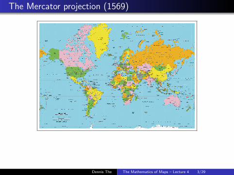
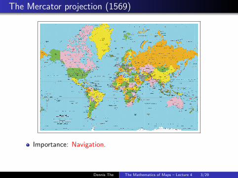
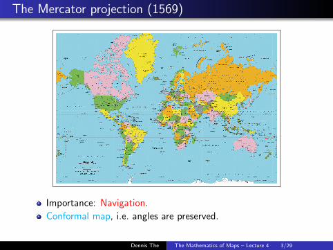
The Mercator projection (1569)
Importance: Navigation.
Conformal map, i.e. angles are preserved.
Here’s a fun little puzzle: Mercator Puzzle
Dennis The The Mathematics of Maps – Lecture 4 3/29
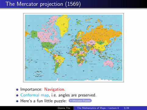
The Mercator projection (1569)
Importance: Navigation.
Conformal map, i.e. angles are preserved.
Here’s a fun little puzzle: Mercator Puzzle
Dennis The The Mathematics of Maps – Lecture 4 3/29
The Mercator projection (1569)
Importance: Navigation.
Conformal map, i.e. angles are preserved.
Here’s a fun little puzzle: Mercator Puzzle
Dennis The The Mathematics of Maps – Lecture 4 3/29
The Mercator projection (1569)
Importance: Navigation.
Conformal map, i.e. angles are preserved.
Here’s a fun little puzzle: Mercator Puzzle
Dennis The The Mathematics of Maps – Lecture 4 3/29

Rhumb lines
Rhumb line = path of constant compass bearing on the sphere, i.e.have constant angle with the corresponding parallel & meridian.
7→
parallels of latitude 7→ horizontal linesmeridians of longitude 7→ vertical linesrhumb lines 7→ straight lines
The last one makes the Mercator map useful for navigation.
Dennis The The Mathematics of Maps – Lecture 4 4/29
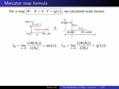
Mercator map formula
For a map Ψ : X = θ, Y = g(φ) , we calculated scale factors:
λp = lims→0
L(Ψ(As))
L(As)= sec(φ), λm = lim
t→0
L(Ψ(Bt))
L(Bt)= |g ′(φ)|.
Conformality means λp = λm . Requiring g(0) = 0, g ′(φ) > 0,
g ′(φ) = sec(φ) ⇒ g(φ) = ln(secφ+ tanφ).
ΨM :
{X = θ, −π ≤ θ ≤ πY = ln(secφ+ tanφ), −π
2 ≤ φ ≤π2
.
Dennis The The Mathematics of Maps – Lecture 4 5/29
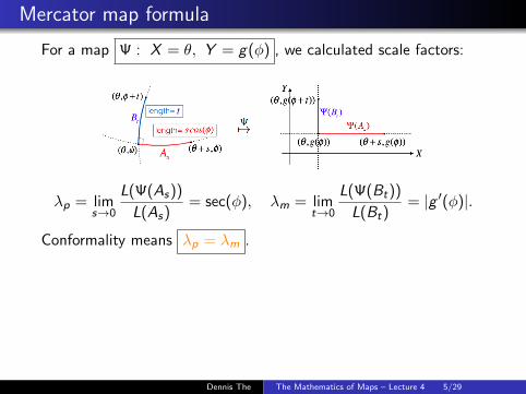
Mercator map formula
For a map Ψ : X = θ, Y = g(φ) , we calculated scale factors:
λp = lims→0
L(Ψ(As))
L(As)= sec(φ), λm = lim
t→0
L(Ψ(Bt))
L(Bt)= |g ′(φ)|.
Conformality means λp = λm .
Requiring g(0) = 0, g ′(φ) > 0,
g ′(φ) = sec(φ) ⇒ g(φ) = ln(secφ+ tanφ).
ΨM :
{X = θ, −π ≤ θ ≤ πY = ln(secφ+ tanφ), −π
2 ≤ φ ≤π2
.
Dennis The The Mathematics of Maps – Lecture 4 5/29

Mercator map formula
For a map Ψ : X = θ, Y = g(φ) , we calculated scale factors:
λp = lims→0
L(Ψ(As))
L(As)= sec(φ), λm = lim
t→0
L(Ψ(Bt))
L(Bt)= |g ′(φ)|.
Conformality means λp = λm . Requiring g(0) = 0, g ′(φ) > 0,
g ′(φ) = sec(φ)
⇒ g(φ) = ln(secφ+ tanφ).
ΨM :
{X = θ, −π ≤ θ ≤ πY = ln(secφ+ tanφ), −π
2 ≤ φ ≤π2
.
Dennis The The Mathematics of Maps – Lecture 4 5/29

Mercator map formula
For a map Ψ : X = θ, Y = g(φ) , we calculated scale factors:
λp = lims→0
L(Ψ(As))
L(As)= sec(φ), λm = lim
t→0
L(Ψ(Bt))
L(Bt)= |g ′(φ)|.
Conformality means λp = λm . Requiring g(0) = 0, g ′(φ) > 0,
g ′(φ) = sec(φ) ⇒ g(φ) = ln(secφ+ tanφ).
ΨM :
{X = θ, −π ≤ θ ≤ πY = ln(secφ+ tanφ), −π
2 ≤ φ ≤π2
.
Dennis The The Mathematics of Maps – Lecture 4 5/29

Mercator map formula
For a map Ψ : X = θ, Y = g(φ) , we calculated scale factors:
λp = lims→0
L(Ψ(As))
L(As)= sec(φ), λm = lim
t→0
L(Ψ(Bt))
L(Bt)= |g ′(φ)|.
Conformality means λp = λm . Requiring g(0) = 0, g ′(φ) > 0,
g ′(φ) = sec(φ) ⇒ g(φ) = ln(secφ+ tanφ).
ΨM :
{X = θ, −π ≤ θ ≤ πY = ln(secφ+ tanφ), −π
2 ≤ φ ≤π2
.
Dennis The The Mathematics of Maps – Lecture 4 5/29
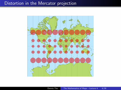
Distortion in the Mercator projection
Dennis The The Mathematics of Maps – Lecture 4 6/29

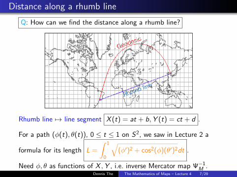
Distance along a rhumb line
Q: How can we find the distance along a rhumb line?
Rhumb line 7→ line segment X (t) = at + b,Y (t) = ct + d .
For a path (φ(t), θ(t)), 0 ≤ t ≤ 1 on S2, we saw in Lecture 2 a
formula for its length L =
∫ 1
0
√(φ′)2 + cos2(φ)(θ′)2dt .
Need φ, θ as functions of X ,Y , i.e. inverse Mercator map Ψ−1M .
Dennis The The Mathematics of Maps – Lecture 4 7/29
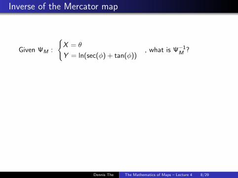
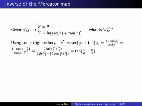
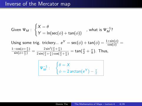
Inverse of the Mercator map
Given ΨM :
{X = θ
Y = ln(sec(φ) + tan(φ)), what is Ψ−1
M ?
Using some trig. trickery... eY = sec(φ) + tan(φ) = 1+sin(φ)cos(φ) =
1−cos(φ+π2
)
sin(φ+π2
) =2 sin2(φ
2+π
4)
2 sin(φ2
+π4
) cos(φ2
+π4
)= tan(φ2 + π
4 ). Thus,
Ψ−1M :
{θ = X
φ = 2 arctan(eY )− π2
Dennis The The Mathematics of Maps – Lecture 4 8/29
Inverse of the Mercator map
Given ΨM :
{X = θ
Y = ln(sec(φ) + tan(φ)), what is Ψ−1
M ?
Using some trig. trickery... eY = sec(φ) + tan(φ) = 1+sin(φ)cos(φ) =
1−cos(φ+π2
)
sin(φ+π2
) =2 sin2(φ
2+π
4)
2 sin(φ2
+π4
) cos(φ2
+π4
)= tan(φ2 + π
4 ).
Thus,
Ψ−1M :
{θ = X
φ = 2 arctan(eY )− π2
Dennis The The Mathematics of Maps – Lecture 4 8/29
Inverse of the Mercator map
Given ΨM :
{X = θ
Y = ln(sec(φ) + tan(φ)), what is Ψ−1
M ?
Using some trig. trickery... eY = sec(φ) + tan(φ) = 1+sin(φ)cos(φ) =
1−cos(φ+π2
)
sin(φ+π2
) =2 sin2(φ
2+π
4)
2 sin(φ2
+π4
) cos(φ2
+π4
)= tan(φ2 + π
4 ). Thus,
Ψ−1M :
{θ = X
φ = 2 arctan(eY )− π2
Dennis The The Mathematics of Maps – Lecture 4 8/29

Distance along a rhumb line - 2
Ψ−1M :
{θ = X
φ = 2 arctan(eY )− π2
,Rhumb
line:
{X (t) = at + b
Y (t) = ct + d
⇒ φ′ =2eY c
1 + e2Y, θ′ = a, cos(φ) =
2eY
1 + e2Y.
L =
∫ 1
0
√(φ′)2 + cos2(φ)(θ′)2dt =
√a2 + c2
∫ 1
0
2eY
1 + e2Ydt
= ... =2√a2 + c2
c(arctan(ec+d)− arctan(ed)) .
(When c → 0, we recover L = 2ed
1+e2d = cos(φ).) This formula is
valid on the unit sphere S2. On a sphere of radius R, this lengthwould be rescaled by R.
Dennis The The Mathematics of Maps – Lecture 4 9/29

Distance along a rhumb line - 2
Ψ−1M :
{θ = X
φ = 2 arctan(eY )− π2
,Rhumb
line:
{X (t) = at + b
Y (t) = ct + d
⇒ φ′ =2eY c
1 + e2Y, θ′ = a, cos(φ) =
2eY
1 + e2Y.
L =
∫ 1
0
√(φ′)2 + cos2(φ)(θ′)2dt =
√a2 + c2
∫ 1
0
2eY
1 + e2Ydt
= ... =2√a2 + c2
c(arctan(ec+d)− arctan(ed)) .
(When c → 0, we recover L = 2ed
1+e2d = cos(φ).)
This formula is
valid on the unit sphere S2. On a sphere of radius R, this lengthwould be rescaled by R.
Dennis The The Mathematics of Maps – Lecture 4 9/29

Distance along a rhumb line - 2
Ψ−1M :
{θ = X
φ = 2 arctan(eY )− π2
,Rhumb
line:
{X (t) = at + b
Y (t) = ct + d
⇒ φ′ =2eY c
1 + e2Y, θ′ = a, cos(φ) =
2eY
1 + e2Y.
L =
∫ 1
0
√(φ′)2 + cos2(φ)(θ′)2dt =
√a2 + c2
∫ 1
0
2eY
1 + e2Ydt
= ... =2√a2 + c2
c(arctan(ec+d)− arctan(ed)) .
(When c → 0, we recover L = 2ed
1+e2d = cos(φ).) This formula is
valid on the unit sphere S2. On a sphere of radius R, this lengthwould be rescaled by R.
Dennis The The Mathematics of Maps – Lecture 4 9/29
Stereographic projection
Dennis The The Mathematics of Maps – Lecture 4 10/29

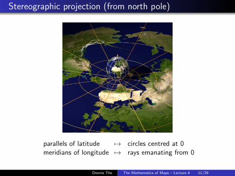
Stereographic projection (from north pole)
parallels of latitude 7→ circles centred at 0meridians of longitude 7→ rays emanating from 0
(Note: Viewed from above, East West is a clockwise rotation in the map.)
Dennis The The Mathematics of Maps – Lecture 4 11/29
Stereographic projection (from north pole)
parallels of latitude 7→ circles centred at 0meridians of longitude 7→ rays emanating from 0
(Note: Viewed from above, East West is a clockwise rotation in the map.)
Dennis The The Mathematics of Maps – Lecture 4 11/29

Stereographic projection (from north pole)
parallels of latitude 7→ circles centred at 0meridians of longitude 7→ rays emanating from 0
(Note: Viewed from above, East West is a clockwise rotation in the map.)
Dennis The The Mathematics of Maps – Lecture 4 11/29

Geometric construction
On S2, put a light source at the north pole, and cast the shadowof ~P ∈ S2 onto the plane tangent at the south pole.
Line ~NP intersects z = −1 plane at ~Q: ( 2x1−z ,
2y1−z ,−1). Hence,
ΨN : X =2x
1− z, Y =
2y
1− z.
Dennis The The Mathematics of Maps – Lecture 4 12/29

Geometric construction
On S2, put a light source at the north pole, and cast the shadowof ~P ∈ S2 onto the plane tangent at the south pole.
Line ~NP intersects z = −1 plane at ~Q: ( 2x1−z ,
2y1−z ,−1).
Hence,
ΨN : X =2x
1− z, Y =
2y
1− z.
Dennis The The Mathematics of Maps – Lecture 4 12/29

Geometric construction
On S2, put a light source at the north pole, and cast the shadowof ~P ∈ S2 onto the plane tangent at the south pole.
Line ~NP intersects z = −1 plane at ~Q: ( 2x1−z ,
2y1−z ,−1). Hence,
ΨN : X =2x
1− z, Y =
2y
1− z.
Dennis The The Mathematics of Maps – Lecture 4 12/29

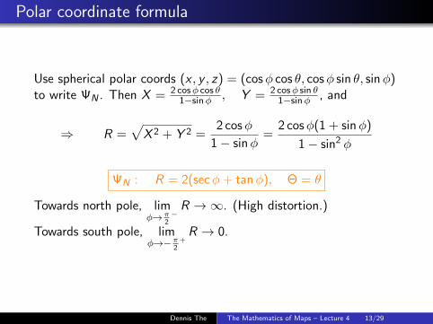
Polar coordinate formula
Use spherical polar coords (x , y , z) = (cosφ cos θ, cosφ sin θ, sinφ)to write ΨN .
Then X = 2 cosφ cos θ1−sinφ , Y = 2 cosφ sin θ
1−sinφ , and
⇒ R =√X 2 + Y 2 =
2 cosφ
1− sinφ=
2 cosφ(1 + sinφ)
1− sin2 φ
ΨN : R = 2(secφ+ tanφ), Θ = θ
Towards north pole, limφ→π
2−R →∞. (High distortion.)
Towards south pole, limφ→−π
2+R → 0.
Dennis The The Mathematics of Maps – Lecture 4 13/29

Polar coordinate formula
Use spherical polar coords (x , y , z) = (cosφ cos θ, cosφ sin θ, sinφ)to write ΨN . Then X = 2 cosφ cos θ
1−sinφ , Y = 2 cosφ sin θ1−sinφ , and
⇒ R =√X 2 + Y 2 =
2 cosφ
1− sinφ=
2 cosφ(1 + sinφ)
1− sin2 φ
ΨN : R = 2(secφ+ tanφ), Θ = θ
Towards north pole, limφ→π
2−R →∞. (High distortion.)
Towards south pole, limφ→−π
2+R → 0.
Dennis The The Mathematics of Maps – Lecture 4 13/29
Stereographic projection is conformal
Halley (1695): Stereographic projection is conformal.
For a map Ψ : R = f (φ), Θ = θ , we calculated scale factors
λp = lims→0
L(Ψ(As))
L(As)= f (φ) sec(φ), λm = lim
t→0
L(Ψ(Bt))
L(Bt)= |f ′(φ)|.
Conformality means λp = λm . For f (φ) = 2(secφ+ tanφ), we
can verify this is true. (Note f ′(φ) > 0 on (−π2 ,
π2 ).)
Dennis The The Mathematics of Maps – Lecture 4 14/29

Distortion in the stereographic projection
Dennis The The Mathematics of Maps – Lecture 4 15/29

Circles are mapped to “circles”
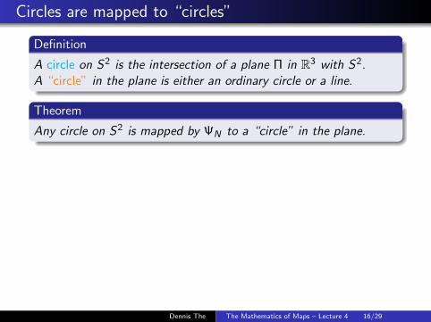
Definition
A circle on S2 is the intersection of a plane Π in R3 with S2.A “circle” in the plane is either an ordinary circle or a line.
Theorem
Any circle on S2 is mapped by ΨN to a “circle” in the plane.
Dennis The The Mathematics of Maps – Lecture 4 16/29
Circles are mapped to “circles”
Definition
A circle on S2 is the intersection of a plane Π in R3 with S2.A “circle” in the plane is either an ordinary circle or a line.
Theorem
Any circle on S2 is mapped by ΨN to a “circle” in the plane.
Dennis The The Mathematics of Maps – Lecture 4 16/29

Circles are mapped to “circles”
Definition
A circle on S2 is the intersection of a plane Π in R3 with S2.A “circle” in the plane is either an ordinary circle or a line.
Theorem
Any circle on S2 is mapped by ΨN to a “circle” in the plane.
Dennis The The Mathematics of Maps – Lecture 4 16/29

Stereographic projection is circle preserving
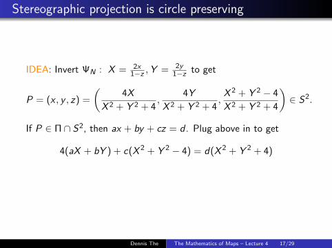
IDEA: Invert ΨN : X = 2x1−z ,Y = 2y
1−z
to get
P = (x , y , z) =
(4X
X 2 + Y 2 + 4,
4Y
X 2 + Y 2 + 4,X 2 + Y 2 − 4
X 2 + Y 2 + 4
)∈ S2.
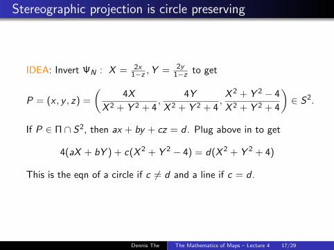
If P ∈ Π ∩ S2, then ax + by + cz = d . Plug above in to get
4(aX + bY ) + c(X 2 + Y 2 − 4) = d(X 2 + Y 2 + 4)
This is the eqn of a circle if c 6= d and a line if c = d .
Dennis The The Mathematics of Maps – Lecture 4 17/29

Stereographic projection is circle preserving
IDEA: Invert ΨN : X = 2x1−z ,Y = 2y
1−z to get
P = (x , y , z) =
(4X
X 2 + Y 2 + 4,
4Y
X 2 + Y 2 + 4,X 2 + Y 2 − 4
X 2 + Y 2 + 4
)∈ S2.
If P ∈ Π ∩ S2, then ax + by + cz = d .
Plug above in to get
4(aX + bY ) + c(X 2 + Y 2 − 4) = d(X 2 + Y 2 + 4)
This is the eqn of a circle if c 6= d and a line if c = d .
Dennis The The Mathematics of Maps – Lecture 4 17/29
Stereographic projection is circle preserving
IDEA: Invert ΨN : X = 2x1−z ,Y = 2y
1−z to get
P = (x , y , z) =
(4X
X 2 + Y 2 + 4,
4Y
X 2 + Y 2 + 4,X 2 + Y 2 − 4
X 2 + Y 2 + 4
)∈ S2.
If P ∈ Π ∩ S2, then ax + by + cz = d . Plug above in to get
4(aX + bY ) + c(X 2 + Y 2 − 4) = d(X 2 + Y 2 + 4)
This is the eqn of a circle if c 6= d and a line if c = d .
Dennis The The Mathematics of Maps – Lecture 4 17/29

Circles images
Dennis The The Mathematics of Maps – Lecture 4 18/29

From Mercator to stereographic projection
Dennis The The Mathematics of Maps – Lecture 4 19/29

A simple complex relationship
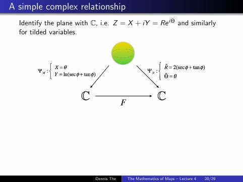
Identify the plane with C, i.e. Z = X + iY = Re iΘ and similarlyfor tilded variables.
The function F is described in real coordinates as
R = 2eY , Θ = X
Using the complex exponential, we have
Z = Re iΘ = 2eY e iX = 2e i(X−iY ) = 2e iZ .
Dennis The The Mathematics of Maps – Lecture 4 20/29
A simple complex relationship
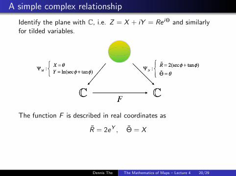
Identify the plane with C, i.e. Z = X + iY = Re iΘ and similarlyfor tilded variables.
The function F is described in real coordinates as
R = 2eY , Θ = X
Using the complex exponential, we have
Z = Re iΘ = 2eY e iX = 2e i(X−iY ) = 2e iZ .
Dennis The The Mathematics of Maps – Lecture 4 20/29

A simple complex relationship
Identify the plane with C, i.e. Z = X + iY = Re iΘ and similarlyfor tilded variables.
The function F is described in real coordinates as
R = 2eY , Θ = X
Using the complex exponential, we have
Z = Re iΘ = 2eY e iX = 2e i(X−iY ) = 2e iZ .
Dennis The The Mathematics of Maps – Lecture 4 20/29

Complex differentiable functions
Given F : C→ C, define C-differentiability via the usual formula
F ′(a) = limh→0
F (a + h)− F (a)
h.
BUT, this is much stronger than
R-differentiability of F considered as a map R2 → R2.
FACT: When F ′ exists and is nonzero, F is a conformal mapping.
The Mercator-to-stereographic map is conformal and decomposes:
Dennis The The Mathematics of Maps – Lecture 4 21/29

Complex differentiable functions
Given F : C→ C, define C-differentiability via the usual formula
F ′(a) = limh→0
F (a + h)− F (a)
h. BUT, this is much stronger than
R-differentiability of F considered as a map R2 → R2.
FACT: When F ′ exists and is nonzero, F is a conformal mapping.
The Mercator-to-stereographic map is conformal and decomposes:
Dennis The The Mathematics of Maps – Lecture 4 21/29
New conformal maps from old
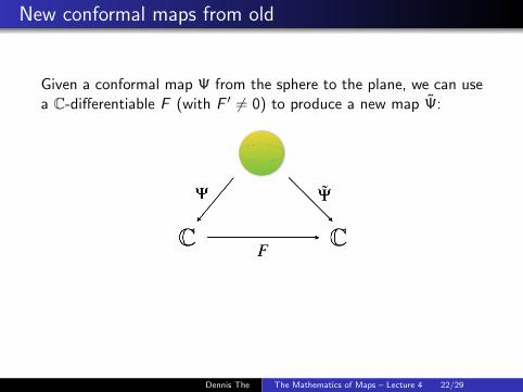
Given a conformal map Ψ from the sphere to the plane, we can usea C-differentiable F (with F ′ 6= 0) to produce a new map Ψ:
Mobius transformations F (z) = az+bcz+d form a wonderful class of
C-differentiable (hence conformal) maps. Mobius transformations revealed
Dennis The The Mathematics of Maps – Lecture 4 22/29

New conformal maps from old
Given a conformal map Ψ from the sphere to the plane, we can usea C-differentiable F (with F ′ 6= 0) to produce a new map Ψ:
Mobius transformations F (z) = az+bcz+d form a wonderful class of
C-differentiable (hence conformal) maps. Mobius transformations revealed
Dennis The The Mathematics of Maps – Lecture 4 22/29

A family of conformal maps
Here’s another way from Mercator to stereographic projection:
The Mercator and stereographic projections, and many in between .Dennis The The Mathematics of Maps – Lecture 4 23/29

Conic conformal projections
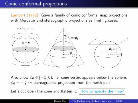
Lambert (1772): Gave a family of conic conformal map projectionswith Mercator and stereographic projections as limiting cases.
Also allow φ0 ∈ [−π2 , 0), i.e. cone vertex appears below the sphere.
φ0 = −π2 stereographic projection from the north pole.
Let’s cut open the cone and flatten it. How to specify the map?
Dennis The The Mathematics of Maps – Lecture 4 24/29

Conic conformal projections
Lambert (1772): Gave a family of conic conformal map projectionswith Mercator and stereographic projections as limiting cases.
Also allow φ0 ∈ [−π2 , 0), i.e. cone vertex appears below the sphere.
φ0 = −π2 stereographic projection from the north pole.
Let’s cut open the cone and flatten it. How to specify the map?
Dennis The The Mathematics of Maps – Lecture 4 24/29

General conic projections
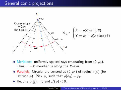
ΨC :
{X = ρ(φ) sin(τθ)
Y = ρ0 − ρ(φ) cos(τθ)
Meridians: uniformly spaced rays emanating from (0, ρ0).Thus, θ = 0 meridian is along the Y -axis.
Parallels: Circular arc centred at (0, ρ0) of radius ρ(φ) (forlatitude φ). Pick φ0 such that ρ(φ0) = ρ0.
Require ρ(π2 ) = 0 and ρ′(φ) < 0.
Dennis The The Mathematics of Maps – Lecture 4 25/29

General conic projections
ΨC :
{X = ρ(φ) sin(τθ)
Y = ρ0 − ρ(φ) cos(τθ)
Meridians: uniformly spaced rays emanating from (0, ρ0).Thus, θ = 0 meridian is along the Y -axis.
Parallels: Circular arc centred at (0, ρ0) of radius ρ(φ) (forlatitude φ). Pick φ0 such that ρ(φ0) = ρ0.
Require ρ(π2 ) = 0 and ρ′(φ) < 0.
Dennis The The Mathematics of Maps – Lecture 4 25/29
General conic conformal projections
Under ΨC , meridians and parallels are orthogonal.
Scale factors:
λp = lims→0
ρ(φ) s2π (2πτ)
s cos(φ)= ρ(φ)τ sec(φ)
λm = limt→0
∣∣∣∣ρ(φ+ t)− ρ(φ)
t
∣∣∣∣ = |ρ′(φ)| = −ρ′(φ)
Conformality λp = λm yields the DE:
ρ′(φ) = −ρ(φ)τ sec(φ), ρ(φ0) = ρ0.
Solving yields
ρ(φ) = ρ0
(secφ0 + tanφ0
secφ+ tanφ
)τ
.
Still have several parameters to play with: ρ0, τ, φ0 .
Dennis The The Mathematics of Maps – Lecture 4 26/29
General conic conformal projections
Under ΨC , meridians and parallels are orthogonal. Scale factors:
λp = lims→0
ρ(φ) s2π (2πτ)
s cos(φ)= ρ(φ)τ sec(φ)
λm = limt→0
∣∣∣∣ρ(φ+ t)− ρ(φ)
t
∣∣∣∣ = |ρ′(φ)| = −ρ′(φ)
Conformality λp = λm yields the DE:
ρ′(φ) = −ρ(φ)τ sec(φ), ρ(φ0) = ρ0.
Solving yields
ρ(φ) = ρ0
(secφ0 + tanφ0
secφ+ tanφ
)τ
.
Still have several parameters to play with: ρ0, τ, φ0 .
Dennis The The Mathematics of Maps – Lecture 4 26/29
Conical maps
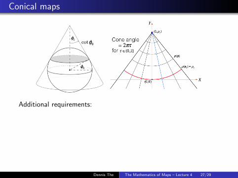
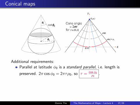
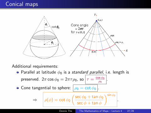
Additional requirements:
Parallel at latitude φ0 is a standard parallel, i.e. length is
preserved. 2π cosφ0 = 2πτρ0, so τ = cosφ0ρ0
.
Cone tangential to sphere: ρ0 = cotφ0 .
⇒ ρ(φ) = cotφ0
(secφ0 + tanφ0
secφ+ tanφ
)sinφ0
.
Dennis The The Mathematics of Maps – Lecture 4 27/29

Conical maps
Additional requirements:
Parallel at latitude φ0 is a standard parallel, i.e. length is
preserved.
2π cosφ0 = 2πτρ0, so τ = cosφ0ρ0
.
Cone tangential to sphere: ρ0 = cotφ0 .
⇒ ρ(φ) = cotφ0
(secφ0 + tanφ0
secφ+ tanφ
)sinφ0
.
Dennis The The Mathematics of Maps – Lecture 4 27/29
Conical maps
Additional requirements:
Parallel at latitude φ0 is a standard parallel, i.e. length is
preserved. 2π cosφ0 = 2πτρ0, so τ = cosφ0ρ0
.
Cone tangential to sphere: ρ0 = cotφ0 .
⇒ ρ(φ) = cotφ0
(secφ0 + tanφ0
secφ+ tanφ
)sinφ0
.
Dennis The The Mathematics of Maps – Lecture 4 27/29

Conical maps
Additional requirements:
Parallel at latitude φ0 is a standard parallel, i.e. length is
preserved. 2π cosφ0 = 2πτρ0, so τ = cosφ0ρ0
.
Cone tangential to sphere: ρ0 = cotφ0 .
⇒ ρ(φ) = cotφ0
(secφ0 + tanφ0
secφ+ tanφ
)sinφ0
.
Dennis The The Mathematics of Maps – Lecture 4 27/29
Conical maps
Additional requirements:
Parallel at latitude φ0 is a standard parallel, i.e. length is
preserved. 2π cosφ0 = 2πτρ0, so τ = cosφ0ρ0
.
Cone tangential to sphere: ρ0 = cotφ0 .
⇒ ρ(φ) = cotφ0
(secφ0 + tanφ0
secφ+ tanφ
)sinφ0
.
Dennis The The Mathematics of Maps – Lecture 4 27/29

Limiting cases
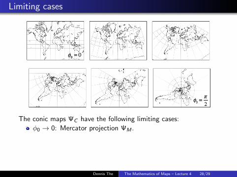
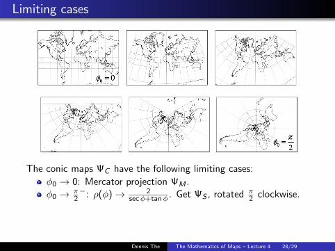
The conic maps ΨC have the following limiting cases:
φ0 → 0: Mercator projection ΨM .φ0 → π
2−: ρ(φ)→ 2
secφ+tanφ . Get ΨS , rotated π2 clockwise.
φ0 → −π2
+: ρ(φ)→ −2(secφ+ tanφ). Get ΨN , rotated π2
clockwise, but then reflected in the X -axis. (Recall: complexconjugation and east west direction was clockwise earlier.)
Dennis The The Mathematics of Maps – Lecture 4 28/29
Limiting cases
The conic maps ΨC have the following limiting cases:
φ0 → 0: Mercator projection ΨM .
φ0 → π2−: ρ(φ)→ 2
secφ+tanφ . Get ΨS , rotated π2 clockwise.
φ0 → −π2
+: ρ(φ)→ −2(secφ+ tanφ). Get ΨN , rotated π2
clockwise, but then reflected in the X -axis. (Recall: complexconjugation and east west direction was clockwise earlier.)
Dennis The The Mathematics of Maps – Lecture 4 28/29
Limiting cases
The conic maps ΨC have the following limiting cases:
φ0 → 0: Mercator projection ΨM .φ0 → π
2−: ρ(φ)→ 2
secφ+tanφ . Get ΨS , rotated π2 clockwise.
φ0 → −π2
+: ρ(φ)→ −2(secφ+ tanφ). Get ΨN , rotated π2
clockwise, but then reflected in the X -axis. (Recall: complexconjugation and east west direction was clockwise earlier.)
Dennis The The Mathematics of Maps – Lecture 4 28/29

Limiting cases
The conic maps ΨC have the following limiting cases:
φ0 → 0: Mercator projection ΨM .φ0 → π
2−: ρ(φ)→ 2
secφ+tanφ . Get ΨS , rotated π2 clockwise.
φ0 → −π2
+: ρ(φ)→ −2(secφ+ tanφ). Get ΨN , rotated π2
clockwise, but then reflected in the X -axis.
(Recall: complexconjugation and east west direction was clockwise earlier.)
Dennis The The Mathematics of Maps – Lecture 4 28/29

Limiting cases
The conic maps ΨC have the following limiting cases:
φ0 → 0: Mercator projection ΨM .φ0 → π
2−: ρ(φ)→ 2
secφ+tanφ . Get ΨS , rotated π2 clockwise.
φ0 → −π2
+: ρ(φ)→ −2(secφ+ tanφ). Get ΨN , rotated π2
clockwise, but then reflected in the X -axis. (Recall: complexconjugation and east west direction was clockwise earlier.)
Dennis The The Mathematics of Maps – Lecture 4 28/29

Broader perspective on these lectures
Q: Given two spaces with some structure, are they equivalent?
The sphere and the plane are
geodesically equivalent;symplectically equivalent (This refers to “area” in dim 2);conformally equivalent.
They are not metrically equivalent. Have Gaussian curvature κ thatis intrinsic and invariant under isometries (“Theorema Egregium”).
A cylinder is metrically equivalent to the plane (also geodesically,symplectically, conformally), i.e. one has ideal maps for a cylinder.
Higher dim? Different structures? Differential geometry!
Dennis The The Mathematics of Maps – Lecture 4 29/29
Broader perspective on these lectures
Q: Given two spaces with some structure, are they equivalent?
The sphere and the plane are
geodesically equivalent;symplectically equivalent (This refers to “area” in dim 2);conformally equivalent.
They are not metrically equivalent.
Have Gaussian curvature κ thatis intrinsic and invariant under isometries (“Theorema Egregium”).
A cylinder is metrically equivalent to the plane (also geodesically,symplectically, conformally), i.e. one has ideal maps for a cylinder.
Higher dim? Different structures? Differential geometry!
Dennis The The Mathematics of Maps – Lecture 4 29/29

Broader perspective on these lectures
Q: Given two spaces with some structure, are they equivalent?
The sphere and the plane are
geodesically equivalent;symplectically equivalent (This refers to “area” in dim 2);conformally equivalent.
They are not metrically equivalent. Have Gaussian curvature κ thatis intrinsic and invariant under isometries (“Theorema Egregium”).
A cylinder is metrically equivalent to the plane (also geodesically,symplectically, conformally), i.e. one has ideal maps for a cylinder.
Higher dim? Different structures? Differential geometry!
Dennis The The Mathematics of Maps – Lecture 4 29/29

Broader perspective on these lectures
Q: Given two spaces with some structure, are they equivalent?
The sphere and the plane are
geodesically equivalent;symplectically equivalent (This refers to “area” in dim 2);conformally equivalent.
They are not metrically equivalent. Have Gaussian curvature κ thatis intrinsic and invariant under isometries (“Theorema Egregium”).
A cylinder is metrically equivalent to the plane (also geodesically,symplectically, conformally), i.e. one has ideal maps for a cylinder.
Higher dim? Different structures? Differential geometry!Dennis The The Mathematics of Maps – Lecture 4 29/29