THE MATHEMATICS OF CAUSAL INFERENCE With ......THE MATHEMATICS OF CAUSAL INFERENCE With reflections on machine learning and the logic of science Judea Pearl UCLA 1. The causal revolution

THE MATHEMATICS OF CAUSAL INFERENCE

With reflections on machine learning and the logic of science

Judea Pearl UCLA

1.  The causal revolution – from statistics to

counterfactuals – from Babylon to Athens

2.  The fundamental laws of causal inference

3.  From counterfactuals to problem solving

a)  policy evaluation (ATE, ETT, …)

b)  attribution

c)  mediation

d)  generalizability – external validity

e)  latent heterogeneity

f)  missing data

OUTLINE

{ {

Old

New

TURING ON MACHINE LEARNING AND EVOLUTION

•  The survival of the fittest is a slow method for measuring advantages.

•  The experimenter, by exercise of intelligence, should be able to speed it up.

•  If he can trace a cause for some weakness he can probably think of the kind of mutation which will improve it. (A.M. Turing, 1950)

THE UBIQUITY OF CAUSAL REASONING

Data-intensive

Scientific applications

Robotics

Human Cognition and

Ethics Thousands of Hungry and

aimless customers Scientific

thinking

AI

Causal Reasoning

Poetry

Arithmetic

Chess

Stock market . . . .

Human Cognition and

Ethics

Causal Reasoning

Poetry

Arithmetic

Chess



AI

Causal Explanation

“She handed me the fruit and I ate”

“The serpent deceived me, and I ate”

COUNTERFACTUALS AND OUR SENSE OF JUSTICE

Abraham: Are you about to smite the righteous with the wicked?

What if there were fifty righteous men in the city?

And the Lord said, “If I find in the city of Sodom fifty good men, I will pardon the whole place for their sake.” Genesis 18:26

Human Cognition and

Ethics

Scientific thinking

Causal Reasoning

Poetry

Arithmetic

Chess



AI

Y = 2X

WHY PHYSICS IS COUNTERFACTUAL

Had X been 3, Y would be 6. If we raise X to 3, Y would be 6. Must “wipe out” X = 1.

X = 1 Y = 2

The solution Process information

Y := 2X

Correct notation:

X = 1

e.g., Length (Y) equals a constant (2) times the weight (X)

Scientific Equations (e.g., Hooke’s Law) are non-algebraic

X = 3 X = ½ Y Y = X+1 Alternative

X = 3

Y ⬅ 2X (or)

Had X been 3, Y would be 6. If we raise X to 3, Y would be 6. Must “wipe out” X = 1.

Correct notation: e.g., Length (Y) equals a constant (2) times the weight (X)

Scientific Equations (e.g., Hooke’s Law) are non-algebraic

WHY PHYSICS IS COUNTERFACTUAL

X = 1 Y = 2

The solution Process information X = 1 X = 3

X = ½ Y Y = X+1 Alternative

X = 3

Robotics

Human Cognition and

Ethics

Scientific thinking

Causal Reasoning

Poetry

Arithmetic

Chess



AI

WHAT KIND OF QUESTIONS SHOULD THE ROBOT ANSWER?

•  Observational Questions: “What if I see A”

•  Action Questions: “What if I do A?”

•  Counterfactuals Questions: “What if I did things differently?”

•  Options: “With what probability?”

Data-intensive

Scientific applications

Robotics

Human Cognition and

Ethics Thousands of Hungry and

aimless customers Scientific

thinking

Causal Reasoning

Poetry

Arithmetic

Chess


AI


TRADITIONAL STATISTICAL INFERENCE PARADIGM

Data

Inference

Q(P) (Aspects of P)

P Joint

Distribution

e.g., Infer whether customers who bought product A would also buy product B. Q = P(B | A)

How does P change to P′? New oracle e.g., Estimate P′(cancer) if we ban smoking.

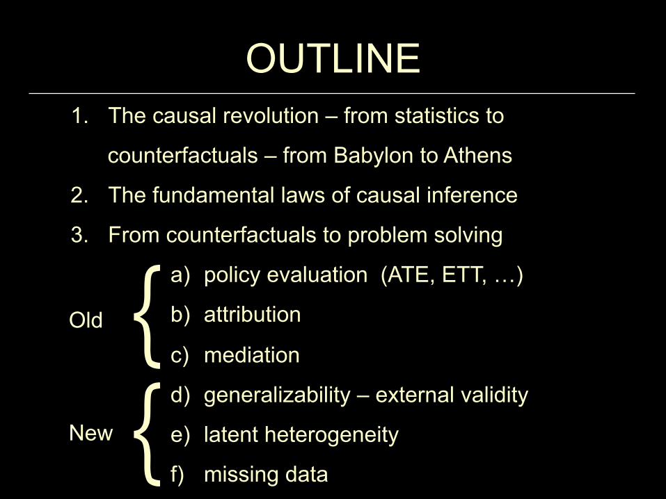
FROM STATISTICAL TO CAUSAL ANALYSIS: 1. THE DIFFERENCES

Data

Inference

Q(P′) (Aspects of P′)

P′ Joint

Distribution

P Joint

Distribution

change

e.g., Estimate the probability that a customer who bought A would buy B if we were to double the price.

FROM STATISTICAL TO CAUSAL ANALYSIS: 1. THE DIFFERENCES

Data

Inference

Q(P′) (Aspects of P′)

P′ Joint

Distribution

P Joint

Distribution

change

Data

Inference

Q(M) (Aspects of M)

Data Generating

Model

M – Invariant strategy (mechanism, recipe, law, protocol) by which Nature assigns values to variables in the analysis.

Joint Distribution

THE STRUCTURAL MODEL PARADIGM

M

“A painful de-crowning of a beloved oracle!” • 

WHAT KIND OF QUESTIONS SHOULD THE ORACLE ANSWER?

•  Observational Questions: “What if we see A”

•  Action Questions: “What if we do A?”

•  Counterfactuals Questions: “What if we did things differently?”

•  Options: “With what probability?”

(What is?)

(What if?)

(Why?)

THE CAUSAL HIERARCHY

P(y | A)

P(y | do(A)

P(yA’ | A)

- SYNTACTIC DISTINCTION

STRUCTURAL CAUSAL MODELS: THE WORLD AS A COLLECTION

OF SPRINGS

Definition: A structural causal model is a 4-tuple <V,U, F, P(u)>, where •  V = {V1,...,Vn} are endogenous variables •  U = {U1,...,Um} are background variables •  F = {f1,..., fn} are functions determining V,

vi = fi(v, u) •  P(u) is a distribution over U P(u) and F induce a distribution P(v) over observable variables

y = α +βx + uYe.g., Not regression!!!!

Definition: The sentence: “Y would be y (in situation u), had X been x,” denoted Yx(u) = y, means: The solution for Y in a mutilated model Mx, (i.e., the equations for X replaced by X = x) with input U=u, is equal to y.

Yx (u) = YMx (u)The Fundamental Equation of Counterfactuals:

COUNTERFACTUALS ARE EMBARRASSINGLY SIMPLE

U

X (u) Y (u)

M U

X = x Yx (u)

Mx

THE TWO FUNDAMENTAL LAWS OF CAUSAL INFERENCE

1.  The Law of Counterfactuals (M generates and evaluates all counterfactuals.)

2.  The Law of Conditional Independence (d-separation) (Separation in the model ⇒ independence in the distribution.)

Yx (u) = YMx (u)

(X sep Y | Z )G(M )⇒ (X ⊥⊥ Y | Z )P(v)

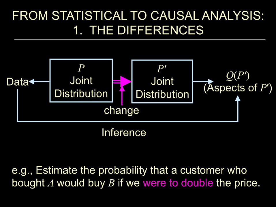
THE LAW OF CONDITIONAL INDEPENDENCE

Each function summarizes millions of micro processes.

C = fC (UC )S = fS (C,US )R = fR(C,UR )W = fW (S,R,UW )

U1

U2

U3

U4

C S

Model (M) C (Climate)

R (Rain)

S (Sprinkler)

W (Wetness)

Graph (G)

Gift of the Gods

If the U 's are independent, the observed distribution P(C,R,S,W) satisfies constraints that are: (1) independent of the f 's and of P(U), (2) readable from the graph.

C (Climate)

R (Rain)

S (Sprinkler)

W (Wetness)

THE LAW OF CONDITIONAL INDEPENDENCE


Graph (G) Model (M)

U1

U2

U3

U4

C S

D-SEPARATION: NATURE’S LANGUAGE FOR COMMUNICATING ITS STRUCTURE

C (Climate)

R (Rain)

S (Sprinkler)

W (Wetness) Every missing arrow advertises an independency, conditional on a separating set.

Applications: 1.  Model testing 2.  Structure learning 3.  Reducing "what if I do" questions to symbolic calculus 4.  Reducing scientific questions to symbolic calculus


e.g., C ⊥⊥ W | (S,R) S ⊥⊥ R |C

Graph (G) Model (M)

SEEING VS. DOING

Effect of turning the sprinkler ON (Truncated product)

P(x1,..., xn ) = P(xi | pai )i∏

P(x1, x2, x3, x4, x5 ) = P(x1)P(x2 | x1)P(x3 | x1)P(x4 | x2, x3)P(x5 | x4 )

PX3=ON(x1, x2, x4, x5 ) = P(x1)P(x2 | x1)P(x4 | x2,X3 = ON)P(x5 | x4 )

≠ P(x1, x2, x4,X5 | X3 = ON)

Q(D,A)

Q(P) - Identified estimands

T(MA) - Testable implications

A* - Logical implications of A

g(T )

Causal inference

Statistical inference

A - CAUSAL ASSUMPTIONS

Q Queries of interest

Data (D)

THE LOGIC OF CAUSAL ANALYSIS

Goodness of fit

Model testing Provisional claims

Q - Estimates of Q(P)

CAUSAL MODEL

(MA)

THE MACHINERY OF CAUSAL CALCULUS

Rule 1: Ignoring observations P(y | do{x}, z, w) = P(y | do{x}, w)

Rule 2: Action/observation exchange

 P(y | do{x}, do{z}, w) = P(y | do{x},z,w)

Rule 3: Ignoring actions

 P(y | do{x}, do{z}, w) = P(y | do{x}, w)

if (Y ⊥⊥ Z | X,W ) GX

if (Y ⊥⊥ Z | X,W )GXZ(W)

if (Y ⊥⊥ Z | X,W )GXZ

Completeness Theorem (Shpitser, 2006)

DERIVATION IN CAUSAL CALCULUS

Smoking Tar Cancer

Probability Axioms

Probability Axioms

Rule 2

Rule 2

Rule 3

Rule 3

Rule 2

Genotype (Unobserved)

P(c | do{s}) = P(c | do{s},t)P(t | do{s})t∑= P(c | do{s},do{t})P(t | do{s})t∑= P(c | do{s},do{t})P(t | s)t∑= P(c | do{t}P(t | s)t∑= P(c | do{t}, s ')P(s ' | do{t})P(t | s)t∑s '∑= P(c | t, s ')P(s ' | do{t})P(t | s)t∑s '∑= P(c | t, s ')P(s ')P(t | s)t∑s '∑

EFFECT OF WARM-UP ON INJURY (After Shrier & Platt, 2008)

No, no!

ATE = ✔ ETT = ✔ PNC = ✔

MATHEMATICALLY SOLVED PROBLEMS

1.  Policy evaluation (ATE, ETT,…)

2.  Attribution

3.  Mediation (direct and indirect effects)

4.  Selection Bias

5.  Latent Heterogeneity

6.  Transportability

7.  Missing Data

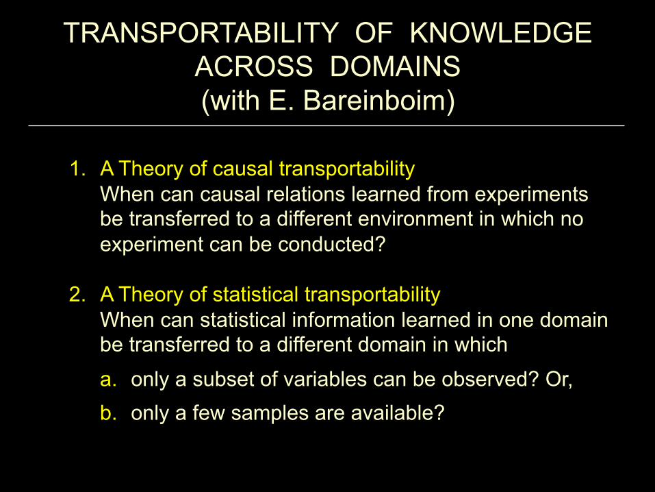
TRANSPORTABILITY OF KNOWLEDGE ACROSS DOMAINS (with E. Bareinboim)

1.  A Theory of causal transportability

When can causal relations learned from experiments be transferred to a different environment in which no experiment can be conducted?

2.  A Theory of statistical transportability When can statistical information learned in one domain be transferred to a different domain in which

a.  only a subset of variables can be observed? Or,

b.  only a few samples are available?

MOVING FROM THE LAB TO THE REAL WORLD . . .

Real world

Everything is assumed to be the same, trivially transportable!

Everything is assumed to be the different, not transportable!

X Y

Z

W

X Y

Z

W

X Y

Z

W Lab H1

H2

MOTIVATION WHAT CAN EXPERIMENTS IN LA TELL ABOUT NYC?

Experimental study in LA Measured:

Needed:

P(x, y, z)P(y | do(x), z)

P*(y | do(x)) = ?

Observational study in NYC Measured: P*(x, y, z)

P*(z) ≠ P(z)

X (Intervention)

Y (Outcome)

Z (Age)

X (Observation)

Y (Outcome)

Z (Age)

= P(y | do(x), z)P*(z)z∑

Transport Formula (calibration):

∏ *∏

F(P,Pdo,P*)

TRANSPORT FORMULAS DEPEND ON THE STORY

a) Z represents age

b) Z represents language skill

P*(y | do(x)) = P(y | do(x), z)P*(z)z∑

P*(y | do(x)) =

X Y Z

(b)

S

X Y

Z

(a)

S

P(y | do(x))?

S

S Factors producing differences

X

TRANSPORT FORMULAS DEPEND ON THE STORY

a) Z represents age

b) Z represents language skill

c) Z represents a bio-marker

P*(y | do(x)) = P(y | do(x), z)P*(z)z∑

P*(y | do(x)) =

X Y Z

(b)

S

(a) X Y

(c) Z

S

P(y | do(x))

P(y | do(x), z)P*(z | x )z∑P*(y | do(x)) = ?

Y

Z S

U

W

GOAL: ALGORITHM TO DETERMINE IF AN EFFECT IS TRANSPORTABLE

X Y Z

V

S T

INPUT: Annotated Causal Graph OUTPUT: 1.  Transportable or not? 2.  Measurements to be taken in the

experimental study 3.  Measurements to be taken in the

target population 4.  A transport formula

S Factors creating differences

P*(y | do(x)) =P *(y,v, z,w,t,u)]f [P(y,v, z,w,t,u | do(x));

S '

= P(y | do(x),w)P(w | s)w∑

= P(y | do(x),w)P*(w)w∑

= P(y | do(x), s,w)P(w | do(x), s)w∑

R *∏( )= P*(y | do(x)) = P(y | do(x), s)

TRANSPORTABILITY REDUCED TO CALCULUS

Theorem A causal relation R is transportable from ∏ to ∏* if and only if it is reducible, using the rules of do-calculus, to an expression in which S is separated from do( ).

X Y

Z

S

W

U

W

RESULT: ALGORITHM TO DETERMINE IF AN EFFECT IS TRANSPORTABLE

X Y Z

V

S T

INPUT: Annotated Causal Graph OUTPUT: 1.  Transportable or not? 2.  Measurements to be taken in the

experimental study 3.  Measurements to be taken in the

target population 4.  A transport formula 5.  Completeness (Bareinboim, 2012)

S Factors creating differences

P*(y | do(x)) =P(y | do(x), z) P *(z |w)

w∑

z∑ P(w | do(w),t)P *(t)

t∑

S '

FROM META-ANALYSIS TO META-SYNTHESIS

The problem How to combine results of several experimental and observational studies, each conducted on a different population and under a different set of conditions, so as to construct an aggregate measure of effect size that is "better" than any one study in isolation.

META-SYNTHESIS AT WORK

X Y

(f) Z

W

X Y

(b) Z

W X Y

(c) Z S

W X Y

(a) Z

W

X Y

(g) Z

W

X Y

(e) Z

W

S S

Target population R = P*(y | do(x))

X Y

(h) Z

W X Y

(i) Z S

W

S

X Y

(d) Z

W

∏*

META-SYNTHESIS REDUCED TO CALCULUS

Theorem {∏1, ∏2,…,∏K} – a set of studies. {D1, D2,…, DK} – selection diagrams (relative to ∏*). A relation R(∏*) is "meta estimable" if it can be decomposed into terms of the form: such that each Qk is transportable from Dk.

Qk = P(Vk | do(Wk ),Zk )

MISSING DATA: A SEEMINGLY STATISTICAL PROBLEM

(Mohan, Pearl & Tian 2012)

•  Pervasive in every experimental science.

•  Huge literature, powerful software industry, deeply entrenched culture.

•  Current practices are based on statistical characterization (Rubin, 1976) of a problem that is inherently causal.

•  Needed: (1) theoretical guidance, (2) performance guarantees, and (3) tests of assumptions.

WHAT CAN CAUSAL THEORY DO FOR MISSING DATA?

Q-1. What should the world be like, for a given statistical procedure to produce the expected result?

Q-2. Can we tell from the postulated world whether any method can produce a bias-free result? How?

Q-3. Can we tell from data if the world does not work as postulated?

•  To answer these questions, we need models of the world, i.e., process models.

•  Statistical characterization of the problem is too crude, e.g., MCAR, MAR, MNAR.

X* =

X if RX = 0m if RX = 1

GOAL: ESTIMATE P(X,Y,Z)

Sam- Observations Missingness ple # X* Y* Z* Rx Ry Rz

1 1 0 0 0 0 0 2 1 0 1 0 0 0 3 1 m m 0 1 1 4 0 1 m 0 0 1 5 m 1 m 1 0 1 6 m 0 1 1 0 0 7 m m 0 1 1 0 8 0 1 m 0 0 1 9 0 0 m 0 0 1

10 1 0 m 0 0 1 11 1 0 1 0 0 0 -

X *

X RX

Missingness graph

{

P(X,Y ,Z ) = P(X,Y ,Z | Rx = 0,Ry = 0,Rz = 0)

Row #

X Y Z Rx Ry Rz

1 1 0 0 0 0 0 2 1 0 1 0 0 0 11 1 0 1 0 0 0 -

•  Line deletion estimate is generally biased.

NAIVE ESTIMATE OF P(X,Y,Z) Complete Cases


1 1 0 0 0 0 0 2 1 0 1 0 0 0 3 1 m m 0 1 1 4 0 1 m 0 0 1 5 m 1 m 1 0 1 6 m 0 1 1 0 0 7 m m 0 1 1 0 8 0 1 m 0 0 1 9 0 0 m 0 0 1

10 1 0 m 0 0 1 11 1 0 1 0 0 0 - Rz Ry Rx

X Y Z

MCAR

P(X,Y ,Z ) ≠ P(X,Y ,Z | Rx = 0,Ry = 0,Rz = 0)

P(X,Y ,Z ) ≠ P(X,Y ,Z | Rx = 0,Ry = 0,Rz = 0)

Row #

X Y Z Rx Ry Rz

1 1 0 0 0 0 0 2 1 0 1 0 0 0 11 1 0 1 0 0 0 -




1 1 0 0 0 0 0 2 1 0 1 0 0 0 3 1 m m 0 1 1 4 0 1 m 0 0 1 5 m 1 m 1 0 1 6 m 0 1 1 0 0 7 m m 0 1 1 0 8 0 1 m 0 0 1 9 0 0 m 0 0 1

10 1 0 m 0 0 1 11 1 0 1 0 0 0 - Rz Rx

X Y Z

MAR

P(X,Y ,Z ) ≠ P(X,Y ,Z | Rx = 0,Ry = 0,Rz = 0)

Row #

X Y Z Rx Ry Rz

1 1 0 0 0 0 0 2 1 0 1 0 0 0 11 1 0 1 0 0 0 -




1 1 0 0 0 0 0 2 1 0 1 0 0 0 3 1 m m 0 1 1 4 0 1 m 0 0 1 5 m 1 m 1 0 1 6 m 0 1 1 0 0 7 m m 0 1 1 0 8 0 1 m 0 0 1 9 0 0 m 0 0 1

10 1 0 m 0 0 1 11 1 0 1 0 0 0 - Rz Rx

X Y Z

MNAR Ry

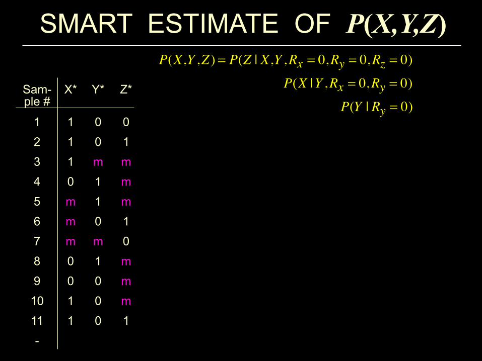
SMART ESTIMATE OF P(X,Y,Z)

P(X,Y ,Z ) = P(Z | X,Y )P(X |Y )P(Y )

P(Y ) = P(Y | Ry = 0)

P(X |Y ) = P(X |Y ,Rx = 0,Ry = 0)

P(Z | X,Y ) = P(Z | X,Y ,Rx = 0,Ry = 0,Rz = 0)

Rz

Ry

Rx

Z X Y


1 1 0 0 0 0 0 2 1 0 1 0 0 0 3 1 m m 0 1 1 4 0 1 m 0 0 1 5 m 1 m 1 0 1 6 m 0 1 1 0 0 7 m m 0 1 1 0 8 0 1 m 0 0 1 9 0 0 m 0 0 1

10 1 0 m 0 0 1 11 1 0 1 0 0 0 -

P(X,Y ,Z ) ≠ P(X,Y ,Z | Rx = 0,Ry = 0,Rz = 0)

P(X,Y ,Z ) = P(Z | X,Y ,Rx = 0,Ry = 0,Rz = 0)

P(X |Y ,Rx = 0,Ry = 0)

P(Y | Ry = 0)Sam-ple #

X* Y* Z*

1 1 0 0 2 1 0 1 3 1 m m 4 0 1 m 5 m 1 m 6 m 0 1 7 m m 0 8 0 1 m 9 0 0 m

10 1 0 m 11 1 0 1 -


P(X,Y ,Z ) = P(Z | X,Y ,Rx = 0,Ry = 0,Rz = 0)

P(X |Y ,Rx = 0,Ry = 0)

P(Y | Ry = 0)Compute P(Y|Ry=0)

Sam-ple #

X* Y* Z*

1 1 0 0 2 1 0 1 3 1 m m 4 0 1 m 5 m 1 m 6 m 0 1 7 m m 0 8 0 1 m 9 0 0 m

10 1 0 m 11 1 0 1 -

Row #

Y*

1 0 2 0 4 1 5 1 6 0 8 1 9 0

10 0 11 0 -


P(X,Y ,Z ) = P(Z | X,Y ,Rx = 0,Ry = 0,Rz = 0)

P(X |Y ,Rx = 0,Ry = 0)

P(Y | Ry = 0)Compute P(X|Y,Rx=0,Ry=0)

Compute P(Y|Ry=0)

Sam-ple #

X* Y* Z*

1 1 0 0 2 1 0 1 3 1 m m 4 0 1 m 5 m 1 m 6 m 0 1 7 m m 0 8 0 1 m 9 0 0 m

10 1 0 m 11 1 0 1 -

Row #

Y*

1 0 2 0 4 1 5 1 6 0 8 1 9 0

10 0 11 0 -

Row #

X* Y*

1 1 0 2 1 0 4 0 1 8 0 1 9 0 0

10 1 0 11 1 0 -


P(X,Y ,Z ) = P(Z | X,Y ,Rx = 0,Ry = 0,Rz = 0)

P(X |Y ,Rx = 0,Ry = 0)

P(Y | Ry = 0)

Compute P(Z|X,Y,Rx=0,Ry=0,Rz=0)

Compute P(X|Y,Rx=0,Ry=0)

Compute P(Y|Ry=0)

Sam-ple #

X* Y* Z*

1 1 0 0 2 1 0 1 3 1 m m 4 0 1 m 5 m 1 m 6 m 0 1 7 m m 0 8 0 1 m 9 0 0 m

10 1 0 m 11 1 0 1 -

Row #

Y*

1 0 2 0 4 1 5 1 6 0 8 1 9 0

10 0 11 0 -

Row #

X* Y*

1 1 0 2 1 0 4 0 1 8 0 1 9 0 0

10 1 0 11 1 0 -

Row #

X* Y* Z*

1 1 0 0 2 1 0 1 11 1 0 1 -


Definition: Given a missingness model M, a probabilistic quantity Q is said to be recoverable if there exists an algorithm that produces a consistent estimate of Q for every dataset generated by M.

That is, in the limit of large sample, Q is estimable as if no data were missing.

RECOVERABILITY FROM MISSING DATA

Theorem: If the missingness-graph is Markovian (i.e., no latent variables) then a necessary and sufficient condition for recoverability of P(V) is that no variable X be adjacent to its missingness mechanism Rx. e.g.,

RECOVERABILITY IN MARKOVIAN MODELS

Z X Y

Ry Rz Rx

Theorem: Q is recoverable iff it is decomposable into terms of the form Qj = P(Sj | Tj) such that Tj contains the missingness mechanism Rv of every partially observed variable V that appears in Q. e.g.,

DECIDING RECOVERABILITY

Rx X Y

(a) Accident Injury

Missing (X) Q1 = P(X,Y ) = P(Y )P(X |Y )

= P(Y )P(X |Y ,Rx )Q2 = P(X) = P(X,Y )y∑

recoverable

recoverable

Theorem: Q is recoverable iff it is decomposable into terms of the form Qj = P(Sj | Tj) such that Tj contains the missingness mechanism Rv of every partially observed variable V that appears in Q. e.g.,

Rx Y X

(b)

Q1 = P(X,Y )

Q2 = P(X)

nonrecoverable

recoverable

≠ P(Y )P(X |Y ,Rx )

= P(X | Rx )

Injury Treatment Education (latent)

Missing (X)

DECIDING RECOVERABILITY

•  Two statistically indistinguishable models, yet P(X,Y) is recoverable in (a) and not in (b).

•  No universal algorithm exists that decides recoverability (or guarantees unbiased results) without looking at the model.

AN IMPOSSIBILITY THEOREM FOR MISSING DATA

Rx X Y

(a) (b)

Rx Y X

Accident Injury Injury Treatment

Missing (X)

Education (latent)

Missing (X)

•  Two statistically indistinguishable models, P(X) is recoverable in both, but through two different methods:

•  No universal algorithm exists that produces an unbiased estimate whenever such exists.

A STRONGER IMPOSSIBILITY THEOREM

Rx X Y

(a) (b)

Rx Y X

In (a): P(X) = P(Y )P(X |Y ,Rx = 0), whiley∑in (b): P(X) = P(X | Rx = 0)

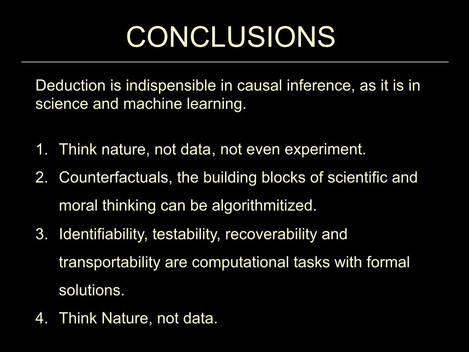
CONCLUSIONS

Deduction is indispensible in causal inference, as it is in science and machine learning.

1.  Think nature, not data

2.  Counterfactuals, the building blocks of scientific and

moral thinking can be algorithmitized.

3.  Identifiability, testability, recoverability and

transportability are computational tasks with formal

solutions.

4.  Think Nature, not data.

, not even experiment.

Thank you

Documents

THE MATHEMATICS OF CAUSAL INFERENCE With ......THE MATHEMATICS OF CAUSAL INFERENCE With reflections on machine learning and the logic of science Judea Pearl UCLA 1. The causal revolution