THE MARKET MODEL OF INTEREST RATE DYNAMICS …

Mathematical Finance, Vol. 7, No. 2 (April 1997), 127–147

THE MARKET MODEL OF INTEREST RATE DYNAMICS 1

ALAN BRACE

Treasury, Citibank, Sydney, Australia

DARIUSZ GATAREK AND MAREK MUSIELA

School of Mathematics, UNSW, Australia

A class of term structure models with volatility of lognormal type is analyzed in the general HJMframework. The corresponding market forward rates do not explode, and are positive and meanreverting. Pricing of caps and floors is consistent with the Black formulas used in the market. Swaptionsare priced with closed formulas that reduce (with an extra assumption) to exactly the Black swaptionformulas when yield and volatility are flat. A two-factor version of the model is calibrated to the U.K.market price of caps and swaptions and to the historically estimated correlation between the forwardrates.

KEY WORDS: term structure models, HJM framework, lognormality of rates, stochastic partialdifferential equations, caps, swaptions

1. INTRODUCTION

In most markets, caps and floors form the largest component of an average swap derivativesbook. A cap/floor is a strip of caplets/floorlets each of which is a call/put option on aforward rate. Market practice is to price the option assuming that the underlying forwardrate process is lognormally distributed with zero drift. Consequently, the option price isgiven by the Black futures formula, discounted from the settlement data.

In an arbitrage-free setting forward rates over consecutive time intervals are related toone another and cannot all be lognormal under one arbitrage-free measure. That probablyis what led the academic community to a degree of skepticism toward the market practiceof pricing caps, and sparked vigorous research with the aim of identifying an arbitrage-freeterm structure model.

The aim of this paper is to show that this market practice can be made consistent with anarbitrage-free term structure model. Consecutive quarterly or semiannual forward rates canall be lognormal while the model will remain arbitrage free. This is possible because eachrate is lognormal under the forward (to the settlement date) arbitrage-free measure ratherthan under one (spot) arbitrage-free measure. Lognormality under the appropriate forwardand not spot arbitrage-free measure is needed to justify the use of the Black futures formulawith discount for caplet pricing. The market seems to interpret the concept of probability

1The authors would like to thank Citibank and the participants of the financial mathematics seminar at theUniversity of New South Wales; mixing of the commercial and academic environments contributed greatly tothis paper. A. Brace and M. Musiela would like to acknowledge the hospitality of the Isaac Newton Institute,where part of this work was carried out. D. G¸atarek is grateful for financial support from the Australian ResearchCouncil.

Address correspondence to Dr. Marek Musiela at the Department of Statistics, School of Mathematics, TheUniversity of New South Wales, Sydney 2052, Australia; e-mail: [email protected].

c© 1997 Blackwell Publishers, 350 Main St., Malden, MA 02148, USA, and 108 Cowley Road, Oxford,OX4 1JF, UK.

127

128 ALAN BRACE, DARIUSZ GATAREK, AND MAREK MUSIELA

distribution in an intuitive rather than mathematical sense, and does not distinguish betweenthe forward measures at different maturities.

We work with the term structure parametrization proposed by Musiela (1993) and laterused by Musiela and Sondermann (1993), Brace and Musiela (1994a), Goldys, Musiela,and Sondermann (1994), and Musiela (1994). We denote byr (t, x) the continuouslycompounded forward rate prevailing at timet over the time interval [t + x, t + x + dx].There is an obvious relationship between the Heath, Jarrow, and Morton (1992) forwardrates f (t, T) and ourr (t, x), namelyr (t, x) = f (t, t + x). For allT > 0 the process

P(t, T) = exp

(−∫ T−t

0r (t, u) du

)= exp

(−∫ T

tf (t, u) du

), 0≤ t ≤ T,

describes price evolution of a zero coupon bond with maturityT . Time evolution of thediscount function

x 7−→ D(t, x) = P(t, t + x) = exp

(−∫ x

0r (t, u) du

)

is described by the processes{D(t, x); t ≥ 0}, x ≥ 0. We make the usual mathematicalassumptions. All processes are defined on the probability space(Ä, {Ft ; t ≥ 0},P), wherethe filtration {Ft ; t ≥ 0} is the P-augmentation of the natural filtration generated bya d-dimensional Brownian motionW = {W(t); t ≥ 0}. We assume that the process{r (t, x); t, x ≥ 0} satisfies

dr(t, x) = ∂

∂x

((r (t, x)+ 1

2|σ(t, x)|2

)dt + σ(t, x) · dW(t)

),(1.1)

where for allx ≥ 0 the volatility process{σ(t, x); t ≥ 0} is Ft -adapted with values inRd, while | | and · stand for the usual norm and inner product inRd, respectively. Wealso assume that the functionx 7−→ σ(t, x) is absolutely continuous and the derivativeτ(t, x) = ∂

∂xσ(t, x) is bounded onR2+ ×Ä. It follows easily that

d D(t, x) = D(t, x) ((r (t, 0)− r (t, x)) dt − σ(t, x) · dW(t)) ,

and henceσ(t, x) can be interpreted as price volatility. Obviously we haveσ(t, 0) = 0.The spot rate process{r (t, 0); t ≥ 0} satisfies

dr(t, 0) = ∂

∂xr (t, x)

∣∣∣∣x=0

dt + ∂

∂xσ(t, x)

∣∣∣∣x=0

· dW(t)

and hence is not Markov, in general. The process

β(t) = exp

(∫ t

0r (s, 0) ds

), t ≥ 0


represents the amount generated at timet ≥ 0 by continuously reinvesting $1 in the spotrater (s, 0), 0≤ s ≤ t .

It is well-known that if for all T > 0 the process{P(t, T)/β(t); 0 ≤ t ≤ T} is amartingale underP then there is no arbitrage possible between the zero coupon bondsP(·, T) of all maturitiesT > 0 and the savings accountβ(·). Note that, under (1.1), wecan easily write that

P(t, T)

β(t)= P(0, T) exp

(−∫ t

0σ(s, T − s) · dW(s)− 1

2

∫ t

0|σ(s, T − s)|2 ds

),(1.2)

where the right-hand side is a martingale. It also follows that

d P(t, T) = P(t, T) (r (t, 0)dt − σ(t, T − t) · dW(t)) .

In Section 2 the existence of the model is established; cap and swaption formulas arederived in Section 3; and, finally, the calibration is described in Section 4.

2. THE MODEL

To specify the model, or equivalently, to define the volatility processσ(t, x) in equation(1.1) we fixδ > 0 (for example,δ = 0.25) and assume that for eachx ≥ 0 the LIBOR rateprocess{L(t, x); t ≥ 0}, defined by

1+ δL(t, x) = exp

(∫ x+δ

xr (t, u) du

),(2.1)

has a lognormal volatility structure; i.e.,

dL(t, x) = · · ·dt + L(t, x)γ (t, x) · dW(t),(2.2)

where the deterministic functionγ : R2+ → Rd is bounded and piecewise continuous. Using

the Ito formula and (1.1) we get

dL(t, x) = δ−1d exp

(∫ x+δ

xr (t, u)du

)= δ−1 exp

(∫ x+δ

xr (t, u) du

)d

(∫ x+δ

xr (t, u) du

)+ δ−1 1

2exp

(∫ x+δ

xr (t, u) du

)|σ(t, x + δ)− σ(t, x)|2 dt

= δ−1 exp

(∫ x+δ

xr (t, u) du

)×((

r (t, x + δ)− r (t, x)+ 1

2|σ(t, x + δ)|2− 1

2|σ(t, x)|2

)dt


+ (σ (t, x + δ)− σ(t, x)) · dW(t)

)+ δ−1 1

2exp

(∫ x+δ

xr (t, u) du

)|σ(t, x + δ)− σ(t, x)|2 dt

=(∂

∂xL(t, x)+ δ−1 (1+ δL(t, x)) σ (t, x + δ)

· (σ (t, x + δ)− σ(t, x))

)dt

+ δ−1 (1+ δL(t, x)) (σ (t, x + δ)− σ(t, x)) · dW(t).

Consequently (2.2) holds for allx ≥ 0 if and only if for all x ≥ 0

σ(t, x + δ)− σ(t, x) = δL(t, x)

1+ δL(t, x)γ (t, x).(2.3)

Under (2.3) the equation forL(t, x) becomes

dL(t, x)=(∂

∂xL(t, x)+L(t, x)γ (t, x)·σ(t, x+δ)

)dt+L(t, x)γ (t, x)·dW(t).(2.4)

Recurrence relationship (2.3) defines the HJM volatility processσ(t, x) for all x ≥ δ

providedσ(t, x) is defined on the interval 0≤ x < δ. We setσ(t, x) = 0 for all 0≤ x < δ

and hence, solving (2.3), we get forx ≥ δ

σ (t, x) =[δ−1x]∑k=1

δL(t, x − kδ)

1+ δL(t, x − kδ)γ (t, x − kδ).(2.5)

Therefore the process{L(t, x); t, x ≥ 0} must satisfy the following equation

dL(t, x) =(∂

∂xL(t, x)+ L(t, x)γ (t, x) · σ(t, x)+ δL2(t, x)

1+ δL(t, x)|γ (t, x)|2

)dt(2.6)

+L(t, x)γ (t, x) · dW(t).

The preceding approach to the term structure modeling is quite different from the tra-ditional one based on the instantaneous continuously compounded spot or forward rates,and therefore we believe its motivations and origins are worth mentioning. The changeof focus from the instantaneous continuously compounded rates to the instantaneous ef-fective annual rates was first proposed by Sandmann and Sondermann (1993) in responseto the impossibility of pricing a Eurodollar futures contract with a lognormal model ofthe instantaneous continuously compounded spot rate. An HJM-type model based on theinstantaneous effective annual rates was introduced by Goldys et al. (1994). A lognormalvolatility structure was assumed on the effective annual ratej (t, x) which is related to the


instantaneous continuously compounded forward rater (t, x) via the formula

1+ j (t, x) = er (t,x).

The case of nominal annual ratesq(t, x) corresponding tor (t, x), i.e.,

(1+ δq(t, x))1/δ = er (t,x)

was studied by Musiela (1994). It turns out that the HJM volatility processσ(t, x) takesthe form

σ(t, x) =∫ x

0δ−1(1− e−δr (t,u))γ (t, u) du.(2.7)

Obviously forδ = 1 we obtain the Goldys et al. (1994) model and forδ = 0 we get

σ(t, x) =∫ x

0r (t, u)γ (t, u) du,

and hence the HJM lognormal model, which is known to explode (forδ > 0 no explosionoccurs).

Unfortunately these models do not give closed form pricing formulas for options. Inorder to price a caplet, for example, one would have to use some numerically intensivealgorithms. This would not be practical for model calibration, where an iterative procedureis needed to identify the volatilityγ (t, x)which returns the market prices for a large numberof caps and swaptions.

A key piece in the term structure puzzle was found by Miltersen, Sandmann, and Son-dermann (1994). First, attention was shifted from the instantaneous ratesq(t, x) to thenominal annual ratesf (t, x, δ) defined by

(1+ f (t, x, δ))δ = exp(∫ x+δ

xr (t, u) du).(2.8)

More importantly, however, it was shown that forδ = 1 the model prices a yearly capletaccording to the market standard. Unfortunately the volatilityσ(t, x) was not completelyidentified, leaving open the question of the model specification for maturities different fromx = i δ and the existence of solution to equation (1.1). These problems were only partiallyaddressed in Miltersen, Sandmann, and Sondermann (1995), where a model based on theeffective ratesf (t, T, δ) defined by

1+ δ f (t, T, δ) = exp

(∫ T+δ−t

T−tr (t, u) du

)(2.9)

was analyzed.


As explained earlier, we assume a lognormal volatility structure on the LIBOR rateL(t, x), defined by (2.1), for allx ≥ 0 and a fixedδ > 0. This leads to the volatilityσ(t, x)given in (2.5) and (2.6) forL(t, x). To prove existence and uniqueness of the solution to(2.6) we need the following result.

LEMMA 2.1. For all x ≥ 0 let{ξ(t, x); t ≥ 0}be an adapted bounded stochastic processwith values inRd, a(·, x): R+ → Rd be a deterministic bounded and piecewise continuousfunction, and let

M(t, x) =∫ t

0a(s, x) · dW(s).

For all x ≥ 0 the equation

dy(t, x) = y(t, x)a(t, x)(2.10)

×((

δy(t, x)

1+ δy(t, x)a(t, x)+ ξ(t, x)

)dt + dW(t)

), y(0, x) > 0,

whereδ > 0 is a constant, has a unique strictly positive solution onR+. Moreover,if for some k∈ {0, 1, 2, . . .}, y(0, ·) ∈ Ck(R+) and for all t ≥ 0, a(t, ·),M(t, ·) andξ(t, ·) ∈ Ck(R+) then for all t≥ 0, y(t, ·) ∈ Ck(R+).

Proof. Since the right-hand side in (2.10) is locally Lipschitz continuous (with respectto y) on R − {−δ−1} and Lipschitz continuous onR+, there exists a unique (possiblyexploding) strictly positive solution to (2.10). By the Ito formula

y(t, x) = y(0, x) exp

(∫ t

0a(s, x) · dW(s)+

∫ t

0a(s, x)(2.11)

·(

δy(s, x)

1+ δy(s, x)a(s, x)+ ξ(s, x)− 1

2a(s, x)

)ds

)

for all t < τ = inf{t : y(t, x) = ∞ or y(t, x) = 0}. But if y(t, x) = 0 for somet <∞ theny(s, x) = 0 for all s ≥ t and henceτ = inf{t : y(t, x) = ∞}. Moreover, because

∫ t

0|a(s, x)|2 ds<∞

for all t <∞ we deduce thatτ = ∞. Thus (2.11) is equivalent to the following Volterra-type integral equation for(t, x) = log y(t, x)

`(t, x) = `(0, x)+∫ t

0a(s, x) · dW(s)(2.12)

+∫ t

0a(s, x) ·

(δe`(s,x)

1+ δe (s,x)a(s, x)+ ξ(s, x)− 1

2a(s, x)

)ds.


Because the right-hand side in (2.12) is globally Lipschitz continuous with respect to`, wededuce using the standard fix-point arguments that there exists a unique pathwise solution toequation (2.12). Moreover for anyt ≥ 0,`(t, ·) ∈ Ck(R+) provided (0, ·), a(t, ·), ξ(t, ·) ∈Ck(R+) for t ≥ 0.

THEOREM2.1. Letγ :R2+ → Rd be a deterministic bounded and piecewise continuous

function,δ > 0 be a constant and let

M(t, x) =∫ t

0γ (s, x + t − s) · dW(s).

Equation (2.6) admits a unique nonnegative solution L(t, x) for any t≥ 0and any nonnega-tive initial condition L(0, ·) = L0. If L0 > 0 then L(t, ·) > 0 for all t > 0. If L0 ∈ Ck(R+)and for all t ≥ 0, γ (t, ·) ∈ Ck(R+), M(t, ·) ∈ Ck(R+), (∂ j /∂x j )γ (t, x)|x=0 = 0,j = 0, 1, . . . , k then for all t≥ 0, L(t, ·) ∈ Ck(R+).

Proof. By the solution to (2.6) we mean the so-called mild solution (cf. Da Prato andZabczyk 1992); i.e.,L(t, x) is a solution if for allt, x ≥ 0

L(t, x) = L(0, x + t)+∫ t

0L(s, x + t − s)γ (s, x + t − s) · σ(s, x + t − s) ds

+∫ t

0

δL2(s, x + t − s)

1+ δL(s, x + t − s)|γ (s, x + t − s)|2 ds

+∫ t

0L(s, x + t − s)γ (s, x + t − s) · dW(s).

This holds true for 0≤ x < δ because the processL(t, x − t), 0 ≤ t ≤ x, x > 0, is asolution to (2.10) witha(t, x) = γ (t, (x − t) ∨ 0) andξ(t, x) = 0. Forδ ≤ x ≤ 2δ theprocessL(t, x − t), 0≤ t ≤ x satisfies (2.10) witha(t, x) = γ (t, (x − t) ∨ 0) and

ξ(t, x) = δL(t, (x − δ − t) ∨ 0)

1+ δL(t, (x − δ − t) ∨ 0).

By induction we prove that equation (2.6) admits a unique solution for anyx > 0 and0 ≤ t ≤ x. Also by induction, using (2.5), we deduce that the correspondinga(t, ·) andξ(t, ·) satisfy the assumptions of regularity in Lemma 2.1 and henceL(t, ·) is smooth aswell.

COROLLARY 2.1. If for some k ∈ N and all t ≥ 0, γ (t, ·) ∈ Ck(R+) and(∂ j /∂x j )γ (t, x)|x=0 = 0, j = 1, . . . , k then equation (1.1) has a unique solution r(t, ·) ∈Ck−1(R+) for any positive initial condition r(0, ·) ∈ Ck−1(R+).


Proof. Consider (1.1) as an equation with fixed volatility processesσ(t, x) given by(2.5) and (2.6).

REMARK 2.1. Volatility σ(t, x) given in (2.5) is not differentiable with respect tox forsome functionsγ (for example, piecewise constant with respect tox). In such a case theterm structure dynamics cannot be analyzed in the HJM framework (1.1). However thisdifficulty is rather technical. Property (1.2) is sufficient to eliminate arbitrage. By puttingT = t in (1.2) we may also use it to define the numeraire (savings account) in terms of theprice volatilityσ . It is also easy to see that for allt ≥ 0

P(t, t + δ) = β(t)P(0, t + δ) exp

(−∫ t

0σ(s, t + δ − s) · dW(s)

− 1

2

∫ t

0|σ(s, t + δ − s|2 ds

)

= β(t)P(0, t + δ) exp

(−∫ t+δ

0σ(s, t + δ − s) · dW(s)

− 1

2

∫ t+δ

0|σ(s, t + δ − s)|2 ds

)= β(t)/β(t + δ)

becauseσ(t, x) = 0 for 0≤ x < δ. Solving the recurrence relationship

β(t + δ) = β(t)P(t, t + δ)−1(2.13)

we get

β(t) =[δ−1t ]∏k=0

P((t − (k+ 1)δ)+, t − kδ)−1.(2.14)

The discounted by{β(t), t ≥ 0} zero coupon bond prices{P(t, T); 0 ≤ t ≤ T} satisfy(1.2) and hence there is no arbitrage.

REMARK 2.2. Regularity ofγ has an important influence on the short rater (t, 0) dynam-ics. If the process{r (t, 0); t ≥ 0} is a semimartingale, then it satisfies

dr(t, 0) = ∂

∂xr (t, x)|x=0dt.(2.15)

Consequently, the short rate is a process of finite variation and therefore it cannot be strongMarkov, except for the deterministic case (cf. ¸Cinlar and Jacod 1981, Remark 3.41). TheLIBOR process{L(t, 0); t ≥ 0} satisfies (2.15) as well.


REMARK 2.3. It follows from (2.11) and Theorem 2.1 that the process{L(t, x); t, x ≥ 0}satisfies

L(t, x) = L(0, x + t) exp

(∫ t

0γ (s, x + t − s) · dW(s)+

∫ t

0γ (s, x + t − s)

·(

δL(s, x + t − s)

1+ δL(s, x + t − s)γ (s, x + t − s)

+ σ(s, x + t − s)− 1

2γ (s, x + t − s)

)ds

)and

|γ (s, x + t − s) · σ(s, x + t − s)| ≤[δ−1(x+t−s)]∑

k=1

|γ (s, x + t − s)|

× |γ (s, x + t − s− kδ)|.

Therefore

L1(t, x) ≤ L(t, x) ≤ L2(t, x),

where

L1(t, x) = L(0, x + t) exp

(∫ t

0γ (s, x + t − s) · dW(s)

−∫ t

0

(α(s, x + t − s)+ 1

2|γ (s, x + t − s)|2

)ds

),

L2(t, x) = L(0, x + t) exp

(∫ t

0γ (s, x + t − s) · dW(s)

+∫ t

0

(α(s, x + t − s)+ 1

2|γ (s, x + t − s)|2

)ds

)while

α(t, x) =[δ−1x]∑k=1

|γ (t, x)||γ (t, x − kδ)|.

Consequently the LIBOR rate is bounded from below and above by lognormal processes.The estimate from above can be used to show that the Eurodollar futures price is welldefined. The most common Eurodollar futures contract relates to the LIBOR rate. Thefutures payoff at timeT is equal toδL(T, 0) and hence the Eurodollar futures price at timet ≤ T is E(δL(T, 0) | Ft ). BecauseL(T, 0) ≤ L2(T, 0) and

E L2(T, 0) = L(0, T) exp

(∫ T

0(α(s, T − s)+ |γ (s, T − s)|2) ds

)<∞,

we conclude that the expectation is finite.


REMARK 2.4. Forn = 1, 2, . . . andt ≥ 0 define

yn(t) = L(t, (nδ − t ∨ 0), γn(t) = γ (t, (nδ = t) ∨ 0)

and assume thatγ (t, 0) = 0. It follows easily that the processes{yn(t); t ≥ 0}, n = 1, 2, . . .satisfy the following closed system of stochastic equations:

dyn(t) = yn(t)γn(t) · n∑

j=[δ−1t ]+1

δyj (t)

1+ δyj (t)γj (t)dt + dW(t)

.

We conclude this section with a study indicating that our model will typically generatemean reverting behavior. Interest rates tend to drop when they are too high and tend to risewhen they are too low. This property, well supported by empirical evidence, is known asmean reversion. We assume that|γ (t, x)| ≤ β(x), where

sup0≤x≤δ

∞∑k=0

β(x + kδ) <∞,(A1)

∫ ∞0(x + 1)β2(x)dx <∞.(A2)

PROPOSITION2.1. Assume (A1)–(A2). Then for any p≥ 1 and any deterministic initialcondition L(0, ·) ∈ Cb(R+)

supt≥0

supx≥0

E Lp(t, x) <∞.

Proof. Letα andL2 be as in Remark 2.3. By (A1) and (A2),

supt≥0

supx≥0

∫ t

0

(α(t, x + t − s)+ 1

2|γ (s, x + t − s)|2

)ds<∞,

and

E

(∫ t

0γ (s, x + t − s) · dW(s)

)2

≤∫ ∞

0β2(x + s) ds≤

∫ ∞0β2(x) dx <∞.

Since logL2 is Gaussian,

supt≥0

supx≥0

E Lp2 (t, x) <∞


for any p ≥ 1. SinceL ≤ L2

supt≥0

supx≥0

E Lp(t, x) < ∞.

Additionally, assume

γ (t, x) = γ (x),(A3)

∫ ∞0

x|γ ′(x)|2 dx <∞,(A4)

sup0≤x≤δ

∞∑k=0

|γ ′(x + kδ)| <∞,(A5)

∫ ∞0|γ (x)| dx = C <

1

K.(A6)

Assumption (A3) implies thatL is a time-homogeneous Markov process. Hence we canstudy the notion of invariant measures. The proof of existence of an invariant measure willfollow the standard Krylov–Bogoliubov scheme: Feller property and tightness of family ofdistributionsL(L(t))t≥0 implies existence of an invariant measure. For details we refer toDaPrato and Zabczyk (1992).

Let C0(R) = {u ∈ C(R): u(x)→ 0 asx→∞} and letCα(R) = {u ∈ C(R): |u(x)−u(z)| ≤ C|x − z|α} for any 0< α ≤ 1. The Holder norm inCα(R) will be denoted by‖ · ‖α. The following result will be useful.

LEMMA 2.2. A family of functions0 ⊂ C0(R+) is relatively compact in C0(R+) if andonly if the following conditions are satisfied:

(i) The family0 is equicontinuous on any bounded set.(ii) There exists a function R:R+ → R+ such that R(u) → 0 as u → ∞ and

| f (u)| ≤ R(u) for any f ∈ 0 and u≥ 0.

THEOREM2.2. Assume (A1)–(A5). Let L be the solution of (2.6) and let

sup0≤x<∞

| log L(0, x)| <∞.

Then

supt≥0

E‖ log L(t)‖ <∞.

If, moreover, (A6) is satisfied than there exists an invariant measure for the process L,concentrated on the closed set

U = {u ∈ C(R) : u > 0 and u(x)→ 1 as x→∞}.


Proof. Consider the processl (t, x) = log L(t, x) which can be represented as

l (x, t) = l0(x + t)+∫ t

0F(l (t − s))(x + t − s) · γ (x + t − s) ds(2.16)

− 1

2

∫ t

0|γ (x + t − s)|2 ds+ M(t, x)

for anyt ≥ 0, whereM is defined by

M(t, x) =∫ t

0γ (x + t − s) · dW(s)

and

F(l )(x) =[δ−1x]∑k=0

δel (x−kδ)

1+ δel (x−kδ)γ (x − kδ)

for anyl ∈ C(R). By (A1), γ · F : C0(R+)→ C0(R+) is a Lipschitz continuous function.By the standard fix-point methodl (t) depends continuously on the initial condition in thespaceC0(R+). Therefore the processl is a Feller process. Notice that

M ′x(t, x) =∫ t

0γ ′(x + t − s) · dW(s).

By the Ito formula

E∫ ∞

0M2(t, x) dx ≤

∫ ∞0

∫ ∞0|γ (x + s)|2 dxds=

√2∫ ∞

0x|γ (x)|2 dx(2.17)

and

E∫ ∞

0M ′x(t, x)2 dx ≤

∫ ∞0

∫ ∞0|γ ′(x + s)|2 dxds=

√2∫ ∞

0x|γ ′(x)|2 dx.(2.18)

By (2.16), fort > 0,

E‖l (t)‖ ≤ ‖l (0)‖ + K∫ ∞

0|γ (x)| dx+ 1

2

∫ ∞0|γ (x)|2 dx+ E sup

x≥0|M(t, x)|.

By (2.17), (2.18), and the Sobolev imbedding

E supx≥u|M(t, x)|2 ≤ C1

(∫ t

0

∫ ∞u|γ (x + s)|2 dxds+

∫ t

0

∫ ∞u|γ ′(x + s)|2 dxds

)≤ R(u) <∞


and for anα < 12

E‖M(t)‖2α ≤ C1

(∫ t

0

∫ ∞0|γ (x + s)|2 dxds+

∫ t

0

∫ ∞0|γ ′(x + s)|2 dxds

)≤ R<∞,

whereR andR(u) are independent oft andR(u)→ 0 asu→∞. Thus

supt≥0

E‖l (t)‖ <∞.

Let (A6) be also satisfied. Assume from now thatl0 = 0. In order to prove existence of aninvariant measure for the processl we will prove that the family of lawsL(l (t))t≥0 is tight.Again by (2.16)

supt≥0

E supx≥u|l (t, x)| ≤ K

∫ ∞u|γ (x)| dx+ 1

2

∫ ∞u|γ (x)|2 dx(2.19)

+ E supx≥u|M(t, x)| → 0

asu→∞. Moreover for anyψ ∈ C(R)

|F(ψ)(x)− F(ψ)(u)||x − u|α ≤ C1+ C K sup

x,u≥0

|ψ(x)− ψ(u)||x − u|α(2.20)

for a certain constantC1. By (A2), (A4), and (A6)

supt≥0

E‖l (t)‖α ≤ C2+ C K supt≥0

E‖l (t)‖α.

SinceC K < 1

supt≥0

E‖l (t)‖α ≤ C2

1− C K.(2.21)

By (2.19), (2.21), and Lemma 2.2, the familyL(l (t))t≥0 is tight onC0(R). Sincel is a Fellerprocess, by the standard Krylov–Bogoliubov technique there exists an invariant measurefor the processl , concentrated onC0(R). Existence of invariant measures forl on C0(R)is equivalent to existence of invariant measures forL onU .

3. DERIVATIVES PRICING

In this section we derive formulas for caps and swaptions at different compounding fre-quencies (for example, quarterly and semiannually).


Consider a payer forward swap on principal 1 settled quarterly in arrears at timesTj =T0 + j δ, j = 1, . . . ,n. The LIBOR rate received at timeTj is set at timeTj−1 at the level(cf. (2.1))

L(Tj−1, 0) = δ−1(P(Tj−1, Tj )−1− 1).

The swap cash flows at timesTj , j = 1, . . . ,n areL(Tj−1, 0)δ and−κδ and hence the timet (t ≤ T0) value of the swap is (cf. Brace and Musiela 1994)

E

(n∑

j=1

β(t)

β(Tj )(L(Tj−1, 0)− κ)δ | Ft

)= P(t, T0)−

n∑j=1

Cj P(t, Tj ),(3.1)

whereCj = κδ for j = 1, . . . ,n− 1 andCn = 1+ κδ.The forward swap rateωT0(t, n) at timet for maturityT0 is that value of the fixed rateκ

which makes the value of the forward swap zero; i.e.,

ωT0(t, n) =(δ

n∑j=1

P(t, Tj )

)−1

(P(t, T0)− P(t, Tn)).(3.2)

In a forward cap (res. floor) on principal 1 settled in arrears at timesTj , j = 1, . . . ,n thecash flows at timesTj are(L(Tj−1, 0) − κ)+δ (res. (κ − L(Tj−1, 0))+δ). The cap price attime t ≤ T0 is

Cap(t) =n∑

j=1

E

(β(t)

β(Tj )(L(Tj−1, 0)− κ)+δ | Ft

)

=n∑

j=1

P(t, Tj )ETj

((L(Tj−1, 0)− κ)+δ | Ft

),

whereET stands for the expectation under the forward measurePT defined by (cf. Musiela(1995))

PT = exp

(−∫ T

0σ(t, T − t) · dW(t)− 1

2

∫ T

0|σ(t, T − t)|2 dt

)P(3.3)

= (P(0, T)β(t))−1P.

The process

K (t, T) = L(t, T − 1) 0≤ t ≤ T(3.4)


satisfies (cf. (2.3) and Theorem 2.1)

dK(t, T) = K (t, T)γ (t, T − t)

·((

δK (t, T)

1+ δK (t, T)γ (t, T − t)+ σ(t, T − t)

)dt + dW(t)

)= K (t, T)γ (t, T − t) · (σ (t, T + δ − t)dt + dW(t)) .

Moreover, the process

WT (t) = W(t)+∫ t

0σ(s, T − s) ds(3.5)

is a Brownian motion underPT . Consequently

dK(t, T) = K (t, T)γ (t, T − t) · dWT+δ(t)(3.6)

and henceK (t, T) is lognormally distributed underPT+δ. It follows that

ET+δ((L(T, 0)− κ)+ | Ft

) = ET+δ((K (T, T)− κ)+ | Ft

)= K (t, T)N(h(t, T))− κN(h(t, T)− ζ(t, T)),

where

h(t, T) =(

logK (t, T)

κ+ 1

2ζ 2(t, T)

)/ζ(t, T),

ζ 2(t, T) =∫ T

t|γ (s, T − s)|2 ds

and hence we have the following result.

PROPOSITION3.1. The cap price at time t≤ T0 is

Cap(t) =n∑

j=1

δP(t, Tj )

× (K (t, Tj−1)N(h(t, Tj−1))− κN(h(t, Tj−1)− ζ(t, Tj−1))).

REMARK 3.1. The preceding Cap(t) formula corresponds to the market Black futuresformula with discount from the settlement date. It was originally derived using a differentapproach and model set-up by Miltersen et al. (1994).

A payer swaption at strikeκ maturing at timeT0 gives the right to receive at timeT0

the cash flows of the corresponding forward payer swap settled in arrears or, alternatively,


discounted from the settlement datesTj = T0 + j δ, j = 1, . . . ,n to T0 value of the cashflows defined by(ωT0(T0, n) − κ)+δ, whereωT0(T0, n) is given in (3.2). Hence the timet ≤ T0 price of the option is

E

(β(t)

β(T0)E

(n∑

j=1

β(T0)

β(Tj )(ωT0(T0, n)− κ)+δ | FT0

)| Ft

)(3.7)

= E

(β(t)

β(T0)

(1−

n∑j=1

Cj P(T0, Tj )

)+| Ft

)

= E

(β(t)

β(T0)

(E

(n∑

j=1

β(T0)

β(Tj )(L(Tj−1, 0)− κ)δ | FT0

))+| Ft

),

whereCj = κδ for j = 1, . . . ,n− 1 andCn = 1+ κδ (cf. Brace and Musiela 1994b). Let

A = {ωT0(T0, n) ≥ κ} ={

n∑j=1

Cj P(T0, Tj ) ≤ 1

}(3.8)

be the event that the swaption ends up in the money. The second expression in (3.7) can bewritten as follows

P(t, T0)PT0(A | Ft )−n∑

j=1

Cj E

(β(t)

β(T0)E

(β(T0)

β(Tj )| FT0

)I A | Ft

)(3.9)

= P(t, T0)PT0(A | Ft )−n∑

j=1

Cj P(t, Tj )PTj (A | Ft ).

Also for all j = 1, . . . ,n

P(t, Tj−1)PTj−1(A | Ft ) = E

(β(t)

β(Tj−1)I A | Ft

)(3.10)

= E

(β(t)

β(Tj )

1

P(Tj−1, Tj )I A | Ft

)= E

(β(t)

β(Tj )(1+ δK (Tj−1, Tj−1))I A | Ft

)= P(t, Tj )PTj (A | Ft )

+ δP(t, Tj )ETj (K (Tj−1, Tj−1)I A | Ft )

= P(t, Tj )PTj (A | Ft )

+ δP(t, Tj )ETj (K (T0, Tj−1)I A | Ft ),


where the last equality holds because the process{K (t, Tj−1); 0≤ t ≤ Tj−1} is a martingaleunder the measurePTj and the eventA is FT0 measurable (see (3.4)–(3.6) and (3.8)).Consequently we have the following result.

THEOREM3.1. The payer swaption price at time t≤ T0 is

Ps(t) = δn∑

j=1

P(t, Tj )ETj

((K (T0, Tj−1)− κ)I A | Ft

).

To simplify further the preceding swaption formula we need to analyze first the rela-tionships between the forward measuresPTj , defined in (3.3), as well as the correspondingforward Brownian motionsWTj , given in (3.5), forj = 1, 2, . . . ,n. We have

dWTj (t) = dW(t)+ σ(t, Tj − t)dt(3.11)

= dWTj−1(t)+ (σ (t, Tj − t)− σ(t, Tj−1− t)) dt

= dWTj−1(t)+δK (t, Tj−1)

1+ δK (t, Tj−1)γ (t, Tj−1− t) dt.

Also, because the process{K (t, Tj−1); 0≤ t ≤ Tj−1} satisfies

dK(t, Tj−1) = K (t, Tj−1)γ (t, Tj−1− t) · dWTj (t),

we have

dδK (t, Tj−1)

1+ δK (t, Tj−1)= δK (t, Tj−1)

(1+ δK (t, Tj−1))2γ (t, Tj−1− t) · dWTj (t)(3.12)

− δ2K 2(t, Tj−1)

(1+ δK (t, Tj−1))3|γ (t, Tj−1− t)|2 dt

= δK (t, Tj−1)

(1+ δK (t, Tj−1))2γ (t, Tj−1− t) · dWTj−1(t),

and hence the process{(1+δK (t, Tj−1))−1δK (t, Tj−1); 0≤ t ≤ Tj−1} is a supermartingale

under the measurePTj and a martingale under the measurePTj−1.Let for t ≤ T0

FT0(t, Tk) = P(t, Tk)

P(t, T0)(3.13)

denote the forward price at timet for settlement at timeT0 on aTk maturity zero couponbond. Because we have

FT0(t, Tk) =k∏

i=1

FTi−1(t, Ti ) =(

k∏i=1

(1+ δK (t, Ti−1))

)−1


the eventA, defined in (3.8), can be written as follows

A = n∑

k=1

Ck

(k∏

i=1

(1+ δK (T0, Ti−1))

)−1

≤ 1

(3.14)

={

n∑k=1

Ck

(k∏

i=1

(1+ δK (t, Ti−1) exp

(∫ T0

tγ (s, Ti−1− s) · dWTi (s)

− 1

2

∫ T0

t|γ (s, Ti−1− s)|2 ds)

))−1

≤ 1

.Moreover, we deduce from (3.11) that fort ≤ T0 andi, j = 1, . . . ,n

dWTi (t) = dWTj (t)+i−1∑`=0

δK (t, T )

1+ δK (t, T )γ (t, T − t) dt(3.15)

−j−1∑`=0

δK (t, T )

1+ δK (t, T )γ (t, T − t) dt.

Consequently we can write

Xi =∫ T0

tγ (s, Ti−1− s) · dWTi (s) =

∫ T0

tγ (s, Ti−1− s) · dWTj (s)(3.16)

+i∑`=1

∫ T0

t

δK (s, T −1)

1+ δK (s, T −1)γ (s, T −1− s) · γ (s, Ti−1− s) ds

−j∑

`=1

∫ T0

t

δK (s, T −1)

1+ δK (s, T −1)γ (s, T −1− s) · γ (s, Ti−1− s) ds.

We will approximate the conditional onFt distribution of X1, . . . , Xn under the measurePTj (for each j = 1, . . . ,n) by the distribution of the random vectorX j

1, . . . , X jn, where

X ji =

∫ T0

tγ (s, Ti−1− s) · dWTj (s)+

i∑`=1

δK (t, T −1)

1+ δK (t, T −1)1ì(3.17)

−j∑

`=1

δK (t, T −1)

1+ δK (t, T −1)1ì

and

1ì =∫ T0

tγ (s, T −1− s) · γ (s, Ti−1− s) ds.(3.18)


In view of (3.12) this approximation corresponds to Wiener chaos order 0 approximationof the process

δK (s, T )

1+ δK (s, T )s ≤ T(3.19)

under the measurePT . A more accurate approximation involving Wiener chaoses of order0 and 1 may be used as well. We found, however, that the contribution of order 1 Wienerchaos is not very significant; so we can simply replace the process (3.19) by its value att informula (3.15) or, because of (3.12), by the conditional expectation underPT −1 givenFt .

Obviously the conditional onFt distribution of X j1, . . . , X j

n under the measurePTj isN(µ j ,1), where1ì is given in (3.18) and

µji =

i∑`=1

δK (t, T −1)

1+ δK (t, T −1)1ì −

j∑`=1

δK (t, T −1)

1+ δK (t, T −1)1ì .(3.20)

In practice the first eigenvalue of the matrix1 is approximately 50 times larger than thesecond, and therefore we can assume that1 is of rank 1, or equivalently that

1ì = 0`0i(3.21)

for some positive constants01, . . . 0n. Setd0 = 0 and fori ≥ 1

di =i∑`=1

δK (t, T −1)

1+ δK (t, T −1)0`,(3.22)

then it follows from (3.20) and (3.21) that

µji = 0i (di − dj ).(3.23)

For all j = 1, . . . ,n the function

f j (x) = 1−n∑

k=1

Ck

(k∏

i=1


(0i (x + di − dj )− 1

202

i

)))−1

satisfiesf ′j (x) > 0, f j (−∞) = −nδκ, f (∞) = 1. Hence there is a unique pointsj suchthat f j (sj ) = 0. Moreover, ifs0 is the solution withj = 0, clearlysj = s0 + dj . Alsof j (x) ≥ 0 for x ≥ sj and therefore, using (3.14), (3.17), and (3.23) we deduce that

PTj (A | Ft ) = PTj (Xjj ≥ 0i sj | Ft ) = N(−s0− dj ).(3.24)


Moreover, standard arguments yield

ETj (K (T0, Tj−1)I A | Ft ) = ETj

(K (t, Tj−1) exp

(∫ T0

tγ (s, Tj−1− s) · dWTj (s)(3.25)

− 1

2

∫ T0

t|γ (s, Tj−1− s)|2 ds

)I A | Ft

)= K (t, Tj−1)N(−s0− dj + 0j )

and finally we obtain the following result.

THEOREM3.2. The price at time t≤ T0 of the payer swaption can be approximated by

Psa(t) = δn∑

j=1

P(t, Tj )(K (t, Tj−1)N(−s0− dj + 0j )− κN(−s0− dj )),

where s0 is given by

n∑k=1

Ck

(k∏

i=1


(0i (s0+ di )− 1

202

i

)))−1

= 1,

Ck = κδ, k = 1, . . . ,n− 1, Cn = 1+ κδ, while0i and di are defined in (3.21) and (3.22)respectively.

Proof. Follows from Theorem 3.1 and formulas (3.24) and (3.25).

In the US, UK, and Japanese markets caps correspond to rates compounded quarterly,while swaptions are semiannual. In the German market caps are quarterly and swaptionsannual. We deal with this problem by assuming lognormal volatility structure on thequarterly rates. The forward swap rate at timet ≤ T0 is

ω(k)T0(t, n) =

(kδ

n∑j=1

P(t, Tkj )

)−1

(P(t, T0)− P(t, Tkn))(3.26)

and hence the timet ≤ T0 price of a payer swaption at strikeκ maturing at timeT0 is

Ps(k)(t) = E

(n∑

j=1

β(t)

β(Tkj )(ω

(k)T0(T0, n)− κ)+kδ | Ft

)

= E

(β(t)

β(T0)

(1−

n∑j=1

C(k)j P(T0, Tkj )

)+| Ft

)

= P(t, T0)PT0(A | Ft )−n∑

j=1

C(k)j P(t, Tkj )PTkj (A | Ft ),


whereC(k)j = kκδ for j = 1, . . . ,n− 1 andC(k)

n = 1+ kκδ, while

A = {ω(k)T0(T0, n) ≥ κ} =

{n∑

j=1

C(k)j P(T0, Tkj ) ≤ 1

}.

From (3.10) it follows that for allj

P(t, Tk( j−1))PTk( j−1) (A | Ft ) = P(t, Tkj )PTkj (A | Ft )

+ δk∑

i=1

P(t, Tk( j−1)+i )ETk( j−1)+i

× (K (T0, Tk( j−1)+i−1)I A | Ft ),

and hence

Ps(k)(t) = δ

n∑j=1

(k j∑

i=k( j−1)+1

P(t, Ti )ETi (K (T0, Ti−1)I A | Ft )(3.27)

− kκP(t, Tkj )PTkj (A | Ft )

).

Repeating arguments used in the proof of Theorem 3.1 we deduce the following swaptionapproximation formula.

THEOREM3.3. Let k andδ be such that(kδ)−1 is the compounding frequency per yearof the swap rateω(k)T0

(t, n), given in (3.26). The time t≤ T0 price of a payer swaption canbe approximated by

Psa(k)(t) = δ

n∑j=1

(k j∑

i=k( j−1)+1

P(t, Ti )K (t, Ti−1)N(−s(k)0 − di + 0i

)(3.28)

− kκP(t, Tkj )N(−s(k)0 − dkj

)),

where s(k)0 is given by

n∑j=1

C(k)j

(k j∏

i=1


(0i

(s(k)0 + di

)− 1

202

i

)))−1

= 1,

C(k)j = kκδ for j = 1, . . . ,n− 1, C(k)

n = 1+ kκδ, and0i and di are defined in (3.21) and(3.22) respectively.


REMARK 3.2. If one choosesδ = 0.25, for example, in a market with quarterly andsemiannual caps and swaptions, then formula (3.28) can be used to price the semiannualcaps and swaptions and hence it can also be used to jointly calibrate to both quarterly andsemiannual volatility inputs.

To analyze differences between the exact swaption value, computed by simulation, andan approximate value computed using formula (3.28) withk = 1 andt = 0, a one-factormodel was fitted to U.S. cap and swaption data on 12 July 1994 generating a typical volatilitystructure. Simulation prices were generated under thePTn forward measure using the exactformula

P(0, Tn)ETn

(n−1∑j=0

Cj

n∏i= j+1

(1+ δK (T0, Ti−1))+ Cn

)+(3.29)

with C0 = 1, Cj = −κδ, j = 1, . . . ,n− 1, Cn = −(1+ κδ) and

K (t, Ti−1) = K (0, Ti−1) exp

(∫ t

0γ (s, Ti−1− s) · dWTi (s)−

1

2

∫ t

0|γ (s, Ti−1− s)|2 ds

),

WTi−1(t) = WTi (t)−∫ t

0

δK (s, Ti−1)

1+ δK (s, Ti−1)γ (s, Ti−1− s) ds.

The preceding equations permit the recursive calculation of the Brownian motionsWT0(t), . . . ,WTn−1(t) for 0 ≤ t ≤ T0. For each simulation ofWTn(t) on [0, T0] thatgives values ofK (T0, Ti−1), i = 1, . . . ,n, substitution in (3.29) gives the correspondingvalue of the swaption. The simulation procedure, which involves Riemann and stochasticintegration steps, was checked by back calculating the cap prices used in parametrization.The simulation prices coincided with the closed form prices calculated using the Cap(0)formula of Proposition 3.1. Table 3.1 gives the swaption prices for a range of strikes, op-tion maturities, and swap lengths. Two standard deviation errors of simulated prices are inbrackets. Bid and ask spreads, estimated by professional dealers at Citibank London, arein the last column.

We also compared formula (3.28) with the market formula for pricing swaptions, basedon assuming the underlying swap rate is lognormal, and given by

δ

n∑j=1

P(0, Tj )(ωT0(0, n)N(h)− κN(h− γ√

T0)),(3.30)

where

h =(

logωT0(0, n)

κ+ 1

2γ 2T0

)/γ√

T0.


TABLE 3.1Accuracy of the FormulaPsa(1)(0)

Option maturity Strike Simulation Psa(1)(0) Spreads× Swap length price

6.00% 159.71(0.25) 160.17 40.25× 2 7.00% 39.62(0.25) 40.39 2.5

8.00% 4.25(0.25) 4.61 26.25% 237.79(0.25) 238.09 5

0.25× 3 7.25% 59.33(0.25) 60.54 3.58.25% 6.11(0.25) 6.75 26.60% 361.24(0.25) 362.72 10

0.25× 5 7.60% 79.49(0.25) 81.16 68.60% 5.84(0.25) 6.39 36.70% 386.34(0.25) 389.79 11

0.5× 5 7.70% 127.34(0.25) 131.43 88.70% 25.99(0.25) 28.12 46.60% 187.23(0.25) 188.56 7

1× 2 7.60% 92.93(0.25) 94.76 58.60% 40.29(0.25) 41.99 36.75% 230.00(0.25) 231.80 10

2× 2 7.75% 140.17(0.25) 142.60 78.75% 80.54(0.25) 82.98 67.50% 359.41(0.26) 363.60 20

2× 5 8.50% 189.24(0.25) 194.47 169.50% 91.64(0.25) 95.79 107.00% 227.75(0.25) 230.28 11

3× 2 8.00% 148.15(0.25) 151.14 89.00% 92.68(0.25) 95.67 67.00% 323.71(0.25) 327.13 16

3× 3 8.00% 204.93(0.25) 208.80 129.00% 123.43(0.25) 127.39 97.00% 502.65(0.40) 506.34 27

5× 5 8.00% 331.56(0.37) 336.90 229.00% 209.39(0.34) 215.33 22

10.00% 127.85(0.31) 133.44 18

The difference between calculated and simulated prices is well within spreads. Allprices are in basis points (1 bp= $100 per $1M face value).

Note that because

En∑

j=1

1

β(Tj )(ωT0(T0, n)− κ)+δ

= δn∑

j=1

P(0, Tj )ETj (ωT0(T0, n)− κ)+


TABLE 3.2Black vs Calculated Price

Option maturity Strike Black Psa(1)(0)× Swap length price

8% 183.88 183.880.25× 1 10% 36.59 36.59

12% 1.35 1.358% 344.05 344.05

1× 2 10% 129.36 129.3512% 34.87 34.878% 748.02 747.97

1× 5 10% 281.24 281.1412% 75.82 75.738% 1204.52 1204.19

1× 10 10% 452.88 452.2012% 122.08 121.608% 473.29 473.21

3× 3 10% 262.20 262.0912% 136.27 136.17

When yield and volatility are flat (10% and 20% respectively)the Black swaption formula andPsa(1)(0) are almost identical.All prices are in basis points (1 bp= $100 per $1M face value).

the market seems to identify the forward measuresPTj , j = 1, . . . ,n with the forwardmeasurePT0 and assumes lognormality of the swap rate processωT0(t, n), 0≤ t ≤ T0 underthe measurePT0. In fact, formula (3.28) reduces to (3.30) ifdi = 0,0i = 11/2

i i = γ√

T0,and K (0, Ti ) = K . We assumed constant 10% yield (compounded quarterly) and 20%volatility in formulas (3.28) and (3.30). Table 3.2 gives the swaption prices.

4. MODEL CALIBRATION

To calibrate the model we used data from the U.K. market for Friday, 3 Feb 95. Marketcash, futures, and swap rates are given in Table 4.1, together with the corresponding zerocoupon discount function (ZCDF). Cap and swaption volatilities, given in Table 4.3 (or4.4), together with the historically estimated correlation between the forward rates, given inTable 4.2, were used to compute the model volatilities. We assumed a two-factor model witha piecewise constant volatility structureγ (t, x) = f (t)γ (x), whereγ (x) = (γ1(x), γ2(x))and f :R+ → R. If f ≡ 1 the volatility is time homogeneous sof represents the termstructure of volatility. Because in the U.K. market caps are quarterly while swaptions aresemiannual, we used the cap formula from Proposition 3.1 withδ = 0.25 and the swaptionformula from Theorem 3.3 withk = 2. Computed volatility functions for 3 Feb 95 are givenin Table 4.3. As a comparison a one-factor normal HJM model was fitted to the same setof data. Normal volatilities for 3 Feb 95 are given in Table 4.4 (formulas 3.2 and 6.1 from


TABLE 4.1GBP Yield Curve for 3 Feb 1995

Market rates

Tenor Rate Tenor Rate

Cash 1 Month 6.68750% Future 18 Dec 96 90.94Cash 2 Month 6.75000% Future 19 Mar 97 90.90Cash 3 Month 6.78125% Future 18 Jun 97 90.88Cash 6 Month 7.12500% Future 17 Sep 97 90.85Cash 9 Month 7.50000% Future 17 Dec 97 90.85Future 15 Mar 95 92.94 Swap 2 year 8.265%Future 21 Jun 95 92.26 Swap 3 year 8.550%Future 20 Sep 95 91.83 Swap 4 year 8.655%Future 20 Dec 95 91.52 Swap 5 year 8.770%Future 20 Mar 96 91.31 Swap 7 year 8.910%Future 19 Jun 96 91.15 Swap 10 year 8.920%Future 18 Sep 96 91.04

Zero Coupon Discount Function (ZCDF)

Tenor: x ZCDF (x) Tenor: x ZCDF (x) Tenor: x ZCDF (x)

0.00000000 1.000000002.37260274 0.82165363 7.00821918 0.539804080.07671233 0.994896052.62191781 0.80338660 7.50684932 0.516755320.10958904 0.992689892.87123288 0.78546824 8.00547945 0.494679150.37808219 0.974222893.12054795 0.76794952 8.50410959 0.473534680.62739726 0.955779233.49863014 0.74363879 9.00547945 0.453176770.87671233 0.936699564.00273973 0.71105063 9.50410959 0.433784391.12602740 0.917305964.49863014 0.6797622210.00821918 0.415016691.37534247 0.897853535.00273973 0.6489580410.50821918 0.397204171.62465753 0.878470625.50136986 0.6203222111.00821918 0.380156171.87397260 0.859275586.01095890 0.5921385211.50821918 0.363839862.12328767 0.840295046.50136986 0.56589374

The zero coupon discount function is calculated from the market rates at various tenors. Intermediate ratescan be found by splining.

TABLE 4.2Forward Rate Correlations for GBP

0 0.25 0.5 1 1.5 2 2.5 3 4 5 7 9

0 1.0000 0.6853 0.5320 0.3125 0.3156 0.2781 0.1835 0.0617 0.1974 0.1021 0.1029 0.05980.25 0.6853 1.0000 0.8415 0.6246 0.6231 0.5330 0.4278 0.3274 0.4463 0.2459 0.3326 0.26250.5 0.5320 0.8415 1.0000 0.7903 0.7844 0.7320 0.6346 0.4521 0.5812 0.3439 0.4533 0.36611 0.3125 0.6246 0.7903 1.0000 0.9967 0.8108 0.7239 0.5429 0.6121 0.4426 0.5189 0.42511.5 0.3156 0.6231 0.7844 0.9967 1.0000 0.8149 0.7286 0.5384 0.6169 0.4464 0.5233 0.42992 0.2781 0.5330 0.7320 0.8108 0.8149 1.0000 0.9756 0.5676 0.6860 0.4969 0.5734 0.47712.5 0.1835 0.4278 0.6346 0.7239 0.7286 0.9756 1.0000 0.5457 0.6583 0.4921 0.5510 0.45813 0.0617 0.3274 0.4521 0.5429 0.5384 0.5676 0.5457 1.0000 0.5942 0.6078 0.6751 0.60174 0.1974 0.4463 0.5812 0.6121 0.6169 0.6860 0.6583 0.5942 1.0000 0.4845 0.6452 0.56735 0.1021 0.2439 0.3439 0.4426 0.4464 0.4969 0.4921 0.6078 0.4845 1.0000 0.6015 0.52007 0.1029 0.3326 0.4533 0.5189 0.5233 0.5734 0.5510 0.6751 0.6452 0.6015 1.0000 0.98899 0.0598 0.2625 0.3661 0.4251 0.4299 0.4771 0.4581 0.6017 0.5673 0.5200 0.9889 1.0000

Forward rates were assumed constant on the intervals between the given terms. One year of data (1994) wasused to calculate this table.


TABLE 4.3Lognormal HJM Fit for 3 Feb 1995

Currency: GBP A-T-M Black Market Average error (%): 0.64

Contract Length strike (%) volatility (%) price (bp) Error (bp) Error (%)

Cap 1 7.88 15.50 27 −0.0 −0.0Cap 2 8.39 17.75 100 2.5 2.5Cap 3 8.64 18.00 185 0.8 0.4Cap 4 8.69 17.75 267 0.3 0.1Cap 5 8.79 17.75 360 −7.4 −2.1Cap 7 8.90 16.50 511 2.5 0.5Cap 10 8.89 15.50 703 −0.0 −0.0

Option maturity× Swap length

Swaption 0.25× 2 8.57 16.75 50 −0.6 −1.2Swaption 0.25× 3 8.75 16.50 73 −0.1 −0.1Swaption 1× 4 9.10 15.50 172 −0.4 −0.2Swaption 0.25× 5 8.90 15.00 103 0.1 0.1Swaption 0.25× 7 9.00 13.75 123 1.6 1.3Swaption 0.25× 10 8.99 13.25 151 −0.1 −0.1Swaption 1× 9 9.12 13.25 271 −1.7 −0.6Swaption 2× 8 9.16 12.75 312 1.2 0.4

Contracts to be fitted are on the left with their at-the-money strikes and market quoted Black volatilities. Pricesand the fit, obtained with the volatility functions below, are on the right. Average error in fitting is 0.64%, and thelargest single error is 2.5%. Note 1 bp= $100 per $M face value.

Tenor: x, t γ1(x) γ2(x) f (t)

0.25 0.09481393 0.12146092 1.000000000.50 0.08498925 0.05117321 1.000000001.00 0.22939966 0.09100802 0.991684481.50 0.19166872 0.02876211 1.003883892.00 0.08232925 0.01172934 1.003883892.50 0.18548202 0.00047705 1.076025933.00 0.13817885 −0.01160086 1.076025934.00 0.08562258 −0.04673283 1.047276425.00 0.14547123 −0.04181446 1.027277997.00 0.08869328 −0.05459175 0.966604309.00 0.04121240 −0.03631021 0.93012459

11.00 0.15206796 −0.16626765 0.81425256Piecewise constant on each internal.

Brace and Musiela (1994a) were used in the process of model calibration). Lognormaland normal HJM model fits, expressed in terms of the market cap and swaption prices, aregiven in Table 4.3 and 4.4, respectively.

Discount functions and volatilities for other days of the week 30 Jan to 3 Feb 1995 areavailable in spreadsheet format on request. The inhomogeneous componentf (t) variesover the first 5 years from 0.934 at 0.5 year on 2 Feb 95 to 1.133 at 2 years on 1 Feb 95.


TABLE 4.4Normal HJM Fit for 3 Feb 1995

Currency: GBP A-T-M Black Market Average error (%): 0.55

Contract Length strike (%) volatility (%) price (bp) Error (bp) Error (%)

Cap 1 7.88 15.50 27 0.00 0.00Cap 2 8.39 17.75 100 2.4 2.4Cap 3 8.64 18.00 185 −0.8 −0.5Cap 4 8.69 17.75 267 −0.2 −0.1Cap 5 8.79 17.75 360 −8.9 −2.5Cap 7 8.90 16.50 511 −5.6 −1.1Cap 10 8.89 15.50 703 1.7 0.2

Option maturity× Swap length

Swaption 0.25× 2 8.57 16.75 50 −0.0 −0.1Swaption 0.25× 3 8.75 16.50 73 0.3 0.5Swaption 1× 4 9.10 15.50 172 0.0 0.0Swaption 0.25× 5 8.90 15.00 103 −0.0 −0.0Swaption 0.25× 7 9.00 13.75 123 −0.2 −0.1Swaption 0.25× 10 8.99 13.25 151 0.1 0.1Swaption 1× 9 9.12 13.25 271 −1.3 −0.5Swaption 2× 8 9.16 12.75 312 −0.2 −0.1

Contracts to be fitted are on the left with their at-the-money strikes and market quoted Black volatilities. Pricesand the fit, obtained with the volatility function below, are on the right. Average error in fitting is 0.55%, and thelargest single error is−2.5%. Note 1 bp= $100 per $M face value.

Normal HJM volatility

Tenor: x σ(x)/x

0.25 0.012365110.50 0.012129891.00 0.012076621.50 0.016929112.00 0.013592113.00 0.013856454.00 0.013846915.00 0.012706417.00 0.01154330

11.00 0.01093066Piecewise constant on each interval.

For maturities beyond 5 years the inhomogeneous component drops to 0.718 at 9 and 11years on 31 Jan 95. The quality of fit can be defined as follows

Fit Error (%)

Tolerable Satisfactory Good

Average error < 2% < 2% < 1%Individual error < 8% < 5% < 3%


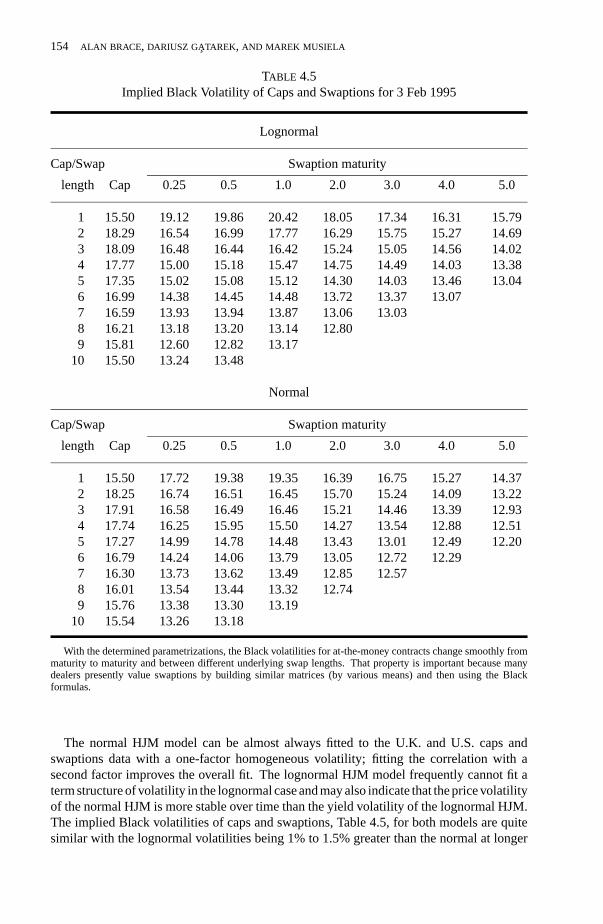
TABLE 4.5Implied Black Volatility of Caps and Swaptions for 3 Feb 1995

Lognormal

Cap/Swap Swaption maturity

length Cap 0.25 0.5 1.0 2.0 3.0 4.0 5.0

1 15.50 19.12 19.86 20.42 18.05 17.34 16.31 15.792 18.29 16.54 16.99 17.77 16.29 15.75 15.27 14.693 18.09 16.48 16.44 16.42 15.24 15.05 14.56 14.024 17.77 15.00 15.18 15.47 14.75 14.49 14.03 13.385 17.35 15.02 15.08 15.12 14.30 14.03 13.46 13.046 16.99 14.38 14.45 14.48 13.72 13.37 13.077 16.59 13.93 13.94 13.87 13.06 13.038 16.21 13.18 13.20 13.14 12.809 15.81 12.60 12.82 13.17

10 15.50 13.24 13.48

Normal

Cap/Swap Swaption maturity

length Cap 0.25 0.5 1.0 2.0 3.0 4.0 5.0

1 15.50 17.72 19.38 19.35 16.39 16.75 15.27 14.372 18.25 16.74 16.51 16.45 15.70 15.24 14.09 13.223 17.91 16.58 16.49 16.46 15.21 14.46 13.39 12.934 17.74 16.25 15.95 15.50 14.27 13.54 12.88 12.515 17.27 14.99 14.78 14.48 13.43 13.01 12.49 12.206 16.79 14.24 14.06 13.79 13.05 12.72 12.297 16.30 13.73 13.62 13.49 12.85 12.578 16.01 13.54 13.44 13.32 12.749 15.76 13.38 13.30 13.19

10 15.54 13.26 13.18

With the determined parametrizations, the Black volatilities for at-the-money contracts change smoothly frommaturity to maturity and between different underlying swap lengths. That property is important because manydealers presently value swaptions by building similar matrices (by various means) and then using the Blackformulas.

The normal HJM model can be almost always fitted to the U.K. and U.S. caps andswaptions data with a one-factor homogeneous volatility; fitting the correlation with asecond factor improves the overall fit. The lognormal HJM model frequently cannot fit aterm structure of volatility in the lognormal case and may also indicate that the price volatilityof the normal HJM is more stable over time than the yield volatility of the lognormal HJM.The implied Black volatilities of caps and swaptions, Table 4.5, for both models are quitesimilar with the lognormal volatilities being 1% to 1.5% greater than the normal at longer


swaption maturities. That probably reflects the different impact of correlation on the twomodels.

REFERENCES

BRACE, A., and M. MUSIELA. (1994a): “A Multifactor Gauss-Markov Implementation of Heath,Jarrow and Morton,”Math. Finance, 2, 259–283.

BRACE, A, and M. MUSIELA. (1994b): “Swap Derivatives in a Gaussian HJM Framework,” preprint,The University of NSW.

CINLAR, E., and J. JACOD. (1981): “Representation of Semimartingale Markov Processes in Termsof Wiener Processes and Poisson Random Measures,” inSeminar on Stochastic Processes, eds.E. Cinlar, K. L. Chung, and R. K. Getoor. Birkhouser, 159–242.

DA PRATO, G, and J. ZABCZYK. (1992): Stochastic Equations in Infinite Dimensions. CambridgeUniversity Press.

GOLDYS B., M. MUSIELA, and D. SONDERMANN. (1994): “Lognormality of Rates and Term StructureModels,” preprint, The University of NSW.

HEATH, D., R. JARROW, and A. MORTON. (1992): “Bond Pricing and the Term Structure of InterestRates: A New Methodology,”Econometrica, 61 (1), 77–105.

MILTERSEN, K., K. SANDMANN , and S. SONDERMANN. (1994): “Closed Form Term Structure Deriva-tives in a Heath-Jarrow-Morton Model with Log-Normal Annually Compounded Interest Rates,”preprint, University of Bonn.

MITTERSEN, K., K. SANDMANN , and D. SONDERMANN. (1995). “Closed Form Solutions for TermStructure Derivatives with Log-Normal Interest Rates,” preprint, University of Bonn.

MUSIELA, M. (1993): “Stochastic PDEs and Term Structure Models.”Journees Internationales deFinance, IGR-AFFI, La Baule.

MUSIELA, M. (1994): “Nominal Annual Rates and Lognormal Volatility Structure,” preprint, TheUniversity of NSW.

MUSIELA, M. (1995): “General Framework for Pricing Derivative Securities,”Stoch. Process Appl.,55, 227–251.

MUSIELA, M., and D. SONDERMANN. (1993): “Different Dinamical Specifications of the Term Struc-ture of Interest Rates and their Implications,” preprint, University of Bonn.

SANDMANN , K., and D. SONDERMANN. (1993): “On the Stability of Lognormal Interest Rate Models,”preprint, University of Bonn.

Documents

THE MARKET MODEL OF INTEREST RATE DYNAMICS …