Stat Comput (2018) 28:1139–1154https://doi.org/10.1007/s11222-017-9784-0

The locally stationary dual-tree complex wavelet model

J. D. B. Nelson1 · A. J. Gibberd2 · C. Nafornita3 · N. Kingsbury4

Received: 15 October 2017 / Accepted: 20 October 2017 / Published online: 26 October 2017© The Author(s) 2017. This article is an open access publication

Abstract We here harmonise two significant contributionsto thefieldofwavelet analysis in thepast twodecades, namelythe locally stationary wavelet process and the family of dual-tree complexwavelets. By combining these two components,we furnish a statistical model that can simultaneously accessbenefits from these two constructions. On the one hand, ourmodel borrows the debiased spectrum and auto-covarianceestimator from the locally stationary wavelet model. On theother hand, the enhanced directional selectivity is obtainedfrom the dual-tree complex wavelets over the regular lattice.The resulting model allows for the description and identi-fication of wavelet fields with significantly more directionalfidelity thanwas previously possible. The corresponding esti-mation theory is established for the new model, and somestationarity detection experiments illustrate its practicality.

J. D. B. Nelson and A. J. Gibberd were supported by Dstl.J. D. B. Nelson was also partially supported by EPSRC GrantEP/N508470/1.

B A. J. Gibberdagibberd@ic.ac.uk

C. Nafornitacorina.nafornita@upt.ro

N. Kingsburyngk@eng.cam.ac.uk

1 Department of Statistical Science, University College, GowerStreet, London WC1E 6BT, UK

2 Department of Mathematics, Imperial College London, SouthKensington Campus, London SW7 2AZ, UK

3 Communications Department, Politehnica University ofTimisoara, Bd. V. Parvan 2, 300223 Timisoara, Romania

4 Department of Engineering, University of Cambridge,Cambridge CB2 1PZ, UK

Keywords Locally stationary wavelet · Random fields ·Dual-tree complex wavelets · Stationarity detection

1 Introduction

This paper has been completed by the second, third and fourthauthors following the untimely death of thefirst author, JamesNelson, in September 2016. It has been submitted for publi-cation in his memory.

Building on the non-stationary time-series work ofDahlhaus (1997) and first proposed by Nason et al. (2000),the locally stationary wavelet (LSW) model provides anovercomplete, translation-invariant representation of a largeclass of non-stationary time series. Unlike many other suchtools, LSW-based methodology affords a statistically well-principled means to capture the local covariance and localspectrum. That auto-covariance estimation of non-stationaryprocesses by any other means comes entangled with var-ious fundamental difficulties has enabled LSW models togain traction across a variety of domains such as forecast-ing for finance (Fryzlewicz 2005); establishing dependenciesin electrophysiological data for neuroscience applications(Sanderson et al. 2010); and spectral estimation of environ-mental time series and ECG traces with missing data (Knightet al. 2012).

Recent years have seen much basic theoretical develop-ment of locally stationary processes. For example, work hasfocussed on: variants of the smoothness constraints placedon the local spectrum function, such as the work by van Bel-legem and von Sachs (2008), Fryzlewicz and Nason (2006),and Nason and Stevens (2015); confidence intervals for theempirical local covariance as recently derived by Nason(2013); and changepoint estimation, such as the work of Kil-lick et al. (2013) and Cho and Fryzlewicz (2015).

123

1140 Stat Comput (2018) 28:1139–1154

Of particular interest here is the extension of the LSW the-ory to two-dimensional processes as recently driven by Eck-ley et al. (2010) and Eckley and Nason (2011). In particular,they extended the result that the local auto-covariance con-verges uniformly to auto-covariance as sample size increasesand that there is an invertible linear mapping from one to theother. This work was subsequently followed by methodol-ogy applied to non-stationarity detection in image textures byTaylor et al. (2014) and segmentation of imagery into station-ary regions by Nunes et al. (2014). A regularised smoothingstrategy for the two-dimensional LSW process is developedin Gibberd and Nelson (2016). Very recently, Taylor et al.(2017) combined the lattice and multivariate extensions toformulate an LSW model for multivalued image data. Assuch, this can be exploited to computemultiscale estimates ofthe local inter-spectral covariance structure of multispectralimagery. The model was then applied to the task of classifi-cation of colour image textures.

The locally stationary wavelet model is hence becom-ing a flexible, extensible means to capture rich behaviourin spatial and image data and to solve practical problems.The overcompleteness of the LSWmodel, compared to, say,decimated wavelet schemes, is a key property which enablesthe LSW to elicit the auto-covariance. The increased numberof wavelet coefficients permits a multiscale sample auto-covariance of sorts to be computed about any point in space.This is problematic in the decimated case since the peri-odogram is computed over the dyadic grid, and as Nasonet al. (2000) notes, the decimated LSWmodel fails to accom-modate all stationary processes (von Sachs et al. 1998). Thiscontrasts with the non-decimated LSW model, which candescribe any stationary process with finite integrated auto-covariance.

Overcompleteness not only affords a feasible means toestimate auto-covariance but also, as a side benefit, resultsin a translation-invariant periodogram. In effect, it providesthe same information as a decimated transform at arbitraryinteger shifts of the input data.

The main thrust of our work herein is to posit that fur-ther overcompletenessmay provide extra value. In particular,when considering random fields such as image data definedover the lattice, directionality can be of significant impor-tance. Often such data present an anisotropic covariancestructure. A simple example of an anisotropic field is illus-trated in Fig. 1. Here the piecewise non-stationarity is dueto a simple relative rotation in the auto-covariance function,between the inner rectangle and outer annulus. In image pro-cessing, the ability to distinguish between such directionalityof textures greatly aids tasks such as classification and seg-mentation.

Unfortunately, traditional real-valued (mono) waveletssuch as the Daubechies family, favoured by the LSW the-ory, possess very limited directionality. This constrains their

AE(90) AE(70)

AE(50) AE(30)

Fig. 1 Anisotropically non-stationary textures drawn fromAE(θ) pro-cess, as defined in Sect. 4.2.2. Processes comprise an inner and outerregion with different orientations, cf. Nelson and Gibberd (2016)

ability to model and represent highly directional phenomenatypical in most modern image processing problems. As such,this has given rise to many so-termed ‘directional wavelets’,including the curvelets of Starck et al. (2002), the contourletsof Do and Vetterli (2002), the steerable pyramids of Portillaand Simoncelli (2000) and the monogenic Riesz–Laplacewavelets of Unser et al. (2009).

We here investigate the incorporation of a special direc-tional wavelet basis, namely the dual-tree complex wavelets(Kingsbury 2001; Selesnick et al. 2005), into the locallystationary wavelet framework. It is shown that, since thesecomplex wavelets are constructed as natural extensions ofreal-valued wavelets, much of the existing LSW theory canbe developed by considering a complex-valued variant of theLSW framework. Indeed, in the sense that the dual-tree com-plexwavelet framework is amultiwavelet tight frame of ordertwo, it can be considered ‘closer’ to the usual real-valuedwavelets than some of the other more exotic and redundantdirectional wavelets, and as such, it provides a natural meansto extend enhanced directionality into the LSW framework.

In Sect. 2, we propose the dual-tree complex locally sta-tionary wavelet processes, denoted hereafter as LSW(C).The processes are real-valued but the definition quite natu-rally permits complex-valued wavelets and transferfunctions—hence extending the usual LSW model.

123

Stat Comput (2018) 28:1139–1154 1141

An additional property, taken straight from dual-tree com-plex wavelet theory, is placed on the relationship betweenthe real and imaginary parts of the wavelet filters. Thisstipulates that they form a Hilbert pair and furnishes thewavelets with directional selectivity and polarity. Theorem1 transfers a central result from the LSW case that the localauto-covariance converges to auto-covariance for LSW(C)

processes.Some estimation theory is covered in Sect. 3. We provide

results that show the LSW(C) periodogram is a biased esti-mator of the spectrum. Furthermore, we establish the resultthat, under reasonable conditions, the biasing matrix canbe inverted; equivalently, the corresponding auto-correlationwavelets retain linear independence; that the spectrum isuniquely defined, given the LSW(C) process; and that themapping between spectrum and covariance is invertible.

In Sect. 4, simulations and experiments on a recent sta-tionarity detectionmethod confirm the utility of the enhanceddirectionality afforded by the proposed model.

Thus, for the first time, ourwork reconciles two significantcontributions to the field of wavelet analysis, combining thelocally stationary wavelet model with the family of dual-treecomplex wavelets.

2 The complex locally stationary wavelet model

The dual-tree complex wavelet transform (Kingsbury 2001;Selesnick et al. 2005) employs a family of carefully con-structed wavelet functions with the remarkable propertythat they jointly maintain approximate translation invari-ance and admit a full multiresolution analysis in the sensethat the resulting two-scale relations are satisfied with finitesequence filters. This enables an implementation of a near-shift-invariant discrete wavelet transform at around the costof two decimated, fast discrete wavelet transforms which canbe computed in parallel.

The two decomposition trees are interpreted as the realand imaginary parts of the complex wavelet coefficients. Thenear-translation-invariance property is achieved by design-ing the wavelet filter sequences in such a way that theyform an approximate Hilbert transform pair—where the realand imaginary parts are 90◦ out of phase with each other.That such invariance is achieved in concert with a genuinemultiresolution analysis places dual-tree wavelets in a veryspecial and unique category in what many refer to informallyas the ‘wavelet zoo’.

In 2-D, the dual-tree scheme also naturally gives riseto improved directionality relative to regular, real-valuedwavelets [such as, for example, Daubechies wavelets usedby Eckley et al. (2010)]. Figure 2 contrasts the directional-ity afforded by a regular, real-valued, discrete 2-D wavelet(or impulse response) function and that of a dual-tree com-

Real DWT

90 045(?)

DT CWT real part

15 45 75 −75 −45 −15(deg)

DT CWT imaginary part

Fig. 2 Dual-tree wavelets provide six directionally selective filters,while real wavelets provide three filters, only two of which have a dom-inant direction

plex wavelet function. The real-valued wavelet functioncomprises filters oriented at 0◦ and 90◦ to the horizontalin addition to a filter oriented at both ± 45◦. This third‘diagonal’ filter will merge together any content oriented at± 45◦—a practitioner will therefore be unable to distinguishbetween these two directions by studying the magnitude ofthe wavelet coefficients. For this reason, at best, one couldperhaps argue that this wavelet function has a directionalityof 2.5.

On the other hand, Fig. 2 also illustrates that the dual-treecomplex wavelets offer six fully directional filters, orientedat {(30� − 15)◦}6�=1. Furthermore, the complex nature of thefilters also yields polarity, or phase, information about imageedges and singularities.

The resultingdual-tree complexwavelet impulse responsesresemble the multiscale directional band-pass filters that theV1 human/mammalian cortical filters use as a front-end pro-cess to their visual systems far more faithfully than thedirectionally limited conventional wavelets—in their experi-mentally ledworkHubel andWiesel (1962) first remarked onthe strong responses to directionality in mammalian visionand, more recently, Ng et al. (2006) provide a review whichincludes a discussion of the analogous role of wavelets withrespect to the underlying biology.

In practice, the directionality offers far richer informationthan the classical, real-valued wavelet functions. As such,dual-tree complex wavelets and their various extensions con-tinue to find hundreds of applications in image modellingand processing areas such as variational Bayesian enhance-ment (Zhang andKingsbury2015), registration and fusion foratmosphere correction (Anantrasirichai et al. 2013), segmen-tation via semi-local scaling exponent estimation (Nelsonet al. 2016), and many more.

123

1142 Stat Comput (2018) 28:1139–1154

Eckley’s 2-D local stationary wavelet (LSW) modeldescribes a stochastic process or field

X =∑

j,�

∑

u

w�j (u) ξ�

j (u) ψ�j (u − ·), (1)

over the finite lattice T := [[1, T ]]2 as a dynamicallyweighted filtering. This combines a real-valued weightingsequence w�

j of a centred orthonormal increment sequence

ξ�j , and an overcomplete basis comprising what Nason et al.

(2000) and Eckley et al. (2010) term (undecimated) ‘discretewavelet functions’ ψ�

j (·) ∈ �2(Z2), indexed over both scale

j and orientation �. As usual, the ‘2-D’ wavelet functionsare separable and are constructed from ‘1-D’ mother andfather wavelets where the discrete mother wavelet functionsare defined by the recursions

ψ j (s) =∑

k

h0(s − 2k) ψ j−1(k), (2)

for j > 0 and s ∈ [[1, T ]], with ψ0(s) = h1(s), wherethe h0 and h1 are, respectively, the low- and high-pass fil-ter sequences of the wavelet ψ . Similar recursions holdfor the father wavelets, cf. Daubechies (1992) and Eckleyet al. (2010). As noted by Nason et al. (2000), these discretewavelet functions are not (necessarily) the result of discretis-ing a continuous wavelet function. In fact, the recursionsdescribed by (2) are equivalent to setting all wavelet coef-ficients, except one at the j th finest scale level, to zero andthen performing an inverse decimatedwavelet transformwithupsampling. Further discussion on the construction of thesesequences, and their numerical generation, can be found in(Daubechies 1992, p. 204).

The LSW can be loosely described as a multiscale,dynamic, moving average model. For only one scale j0 anddirection �0, say, the LSW becomes a moving average modelwith weights that can evolve over space via the sequencew = {w(k)}k . If, in addition, the weights are constant overspacew = w0, say, then the LSW collapses down to a simplemoving average model with parameters {w0ψ

�0j0

(k)}k .For the sake of controlling notational clutter, we fuse the

scale and orientation indexes into one single index η =η( j, �) ∈ H ≡ {1, . . . , 6J }. Without loss of generality, putη = j + (� − 1)J , for j ∈ [[1, J ]].

We further note that the LSW can be equivalently statedin terms of convolutions X = ∑

η∈H wηξη ∗ψη,where the ·denotes a left-right and up-down spatial flip: ϕ := ϕ(−·).Aside from providing an alternative convenient means ofconceptualising the model, introducing such operator nota-tion also helps mitigate notational clutter in some of the laterproofs.

Definition 1 places further constraints on how quickly theweighting sequence can vary over the spatial support. We

here transfer all of the basic real-valued LSW modellingassumptions in Nason et al. (2000) and Eckley et al. (2010)over to our (dual-tree) complexwavelet case. The differencesare that (i) the transfer sequences w and transfer functionsW , below, are now complex-valued, and (ii) Property 5 isadded in order to exploit the approximate Hilbert transformpair property of the dual-tree complex wavelets and there-fore produce wavelets which are directionally selective andwhich carry phase information.

Unlike the LSW model, the DTCWT, as originallydesigned, is decimated. Instead, we here incorporate a non-decimated version of the DTCWT into the LSW. Althoughthe resulting extra computation has little affect on transla-tion invariance (the DTCWT is already near-shift invariant),the dual-tree complex wavelets do greatly enhance the poordirectional description suffered by the LSW model and thenon-decimated construction provides a simple mechanism tointroduce them into the LSW framework. Undecimated ver-sions of the DTCWT have recently been proposed by Hillet al. (2015) who, in addition, note the added virtues thatthe resulting wavelet coefficients are truly co-located overthe scale levels rather than lying on the usual dyadic grid.Although we do note that a big attraction of the DTCWT isthe ability to perform a decimated transform, the incorpora-tion of decimation, partially or wholly, into the LSW is leftas further work for now.

Definition 1 The locally stationary dual-tree complexwavelet stationary processes are defined as the class LSW(C)

of all stochastic processes X : T �→ R over the finite latticeT := [[1, T ]]2 which satisfy the following representation inthe mean-squared sense:

X =∑

η∈Hwηξη ∗ ψη,

with complex-valued sequences wη ∈ �2(T ), centredorthonormal increment processes ξη : T �→ R, discretecomplex wavelet functions ψη : T �→ C, and where thereexist functions Wη : T

2 := (0, 1)2 �→ C, and constantsCη, λη ∈ R such that all the following properties hold for allη ∈ H.

1. supt∈T |wη(t) − Wη(t/T )| ≤ Cη/T , with∑

η Cη < ∞.2. W is square-summable over the scale-orientation indexes:∑

η|Wη(z)|2 < ∞, uniformly in z ∈ T2.

3. Wη is L1-Lipschitz, viz.

∥∥∥∥Wη

(k + ·T

)− Wη

( ·T

)∥∥∥∥L1(R2)

≤ λη‖k/T ‖1

4. The Lipschitz constants λη are uniformly bounded in η

and∑

�

∑j∈N 22 jλη( j,�) < ∞.

123

Stat Comput (2018) 28:1139–1154 1143

5. The complex wavelet functions satisfy the approximateHilbert pair property, cf. Kingsbury (2003) and Selesnicket al. (2005), in that its real ψ·;0 and imaginary ψ·;1 partssatisfy: ψ = ψ·;0 + iψ·;1, with ψ·;0, ψ·;1 : T �→ R,and where the associated filter sequences hab satisfy thebelow properties, where b = 0 or b = 1 signifies thelow-pass or high-pass band sequences, respectively, andwhere a = 0 denotes the real part of the tree and a = 1the imaginary part of the tree:

ha1(k) = (−1)t ha0(n − k), (3)

h10(k) = h00(n − 1 − k), (4)

and where n is the length of the filter sequence.

Note that the approximate Hilbert pair property betweenψ.;0and ψ.;1 ensures that the negative half of the spectrum of ψ

becomes approximately zero. This is the key to obtainingdirectionally selective filters in 2-D from separable 1-D fil-ters, as explained in Selesnick et al. (2005).

The collection of functions {Wη} comprise the parame-ters of the LSW model. They determine how much auto-correlation is present at each scale level. As T → ∞ andthe number of sample points increases, then properties 1 and2 above associate the collection of transfer sequences {wη}with, what become, the bounded family of transfer functions{Wη}. Properties 3 and 4 stipulate that the transfer functionshould be smooth.Asymptotically, theweights are associatedwith Lipschitz continuous functions Wη : T2 �→ C, definedover rescaled space z = t/T , t ∈ T . This condition restrictsthe variation of the weights over space and thus captures thefact that the local structure becomes more stationary whenobserved over evermore smaller spatial neighbourhoods.

A central premise, and unique selling point, of the LSWmodel is that it very naturally offers access to a measureof local covariance via the local spectrum and the auto-correlation wavelet.

Definition 2 (Complex ACW ) Let the superscript · denotecomplex conjugation. Define the (complex) auto-correlationwavelet ACW associated with the possibly complex-valued,discrete wavelet ψ : N2 �→ C by

Ψη = ψη ∗ ψη =

∑

t∈Tψ

η(t)ψη(· + t). (5)

Definition 3 (Local wavelet spectrum) Let X ∈ LSW(C)

have transfer functions Wη : T2 �→ C. Then, the local

wavelet spectrum (LWS) of X is defined by

Sη(·) := |Wη(·)|2 .

Definition 4 (Local auto-correlation) Let S be the localwavelet spectrum, defined by Definition 3, of an LSW(C)

process (Definition 1) and let Ψ be the auto-correlationwavelet as described by Definition 2. Then, the local covari-ance is defined by

C(z, t) =∑

η∈HSη(z)Ψη(t), z ∈ T

2, t ∈ Z2.

A remarkable property is that this local covariance forms agood estimate for the auto-covariance of the, possibly non-stationary, LSW process. The next result establishes this factfor the locally stationary dual-tree complex wavelet pro-cesses.

Theorem 1 (Convergence of auto-covariance) Let C andCT be, respectively, the local auto-covariance and auto-covariance of an LSW process X ∈ LSW(C). Then

|CT (z, t) − C(z, t)|= O(T−1).

as T → ∞, uniformly in t ∈ Z2, and z ∈ T

2.

Remark 1 (Complex extension of the LSW) For X ∈LSW(C):

1. The auto-correlation wavelet is defined via the naturalcomplex extension of the auto-correlation operator.

2. The local wavelet spectrum quantity works in much thesame way as it does in the real LSW case only now it isformed by computing the complex modulus of the trans-fer function.

3 Estimation theory

The (local wavelet) spectrum S represents: the parameters ofthe LSW(C); the amount of ‘energy’ present at a particularscale and orientation; and, via Theorem 1 the spectrum alsoestablishes the second-order behaviour of the field. Two keyquestions naturally follow. The first is how the spectrum canbe estimated and, second, is whether the spectrum is uniquelydefined, given a field.

The (undecimated) local wavelet periodogram (LWP)

X∼η (·) :=

∣∣∣X ∗ ψη

∣∣∣2offers a straightforward but naive esti-

mate of the spectrum. As Theorem 2 shows, the redundancyin the LWS model spreads content, via a so-termed biasingmatrix across the periodogram scales.

Definition 5 (LS-DTCW biasing matrix) Let Ψ be the com-plex ACW as above. Then, the associated biasing matrix is

Aη,ν = 〈Ψη,Ψν〉 =∑

t

Ψη(t)Ψν (t). (6)

123

1144 Stat Comput (2018) 28:1139–1154

Theorem 2 (Periodogram bias) Let the LSW(C) processX : T �→ R, defined on the lattice T := [[1, T ]]2, haveperiodogram X∼

η :=∣∣∣X ∗ ψ

η

∣∣∣2, where {ψη}η∈H is a dis-

crete, undecimated, dual-tree complex wavelet basis and letA be the associated biasing matrix. Then

EX∼η =

∑

ν

AηνSν

( ·T

)+ O(T−1) (7)

The biasing matrix is the agent of this spread or mixing ofredundancy. Note that Definition 5 is but the complex exten-sion of the inner product used to define the real biasingmatrixof the locally stationary, real-valued, wavelet model. In addi-tion to facilitating some subsequent results, it is perhaps ofintrinsic interest to note that the biasingmatrix is real-valued.

Lemma 1 (Bias is real) LetΨ be the ACW (Definition 2. Theentries of the biasing matrix (Definition 5) are positive, real,and symmetric.

Remark 2 (Unbiased spectrum estimator) If the biasingmatrix is invertible, then one can derive an unbiased estimateof the spectrum via:

Sη(z) =∑

ν

A−1η,ν X∼

ν (z). (8)

The consistencyof the smoothedversion of the real-valuedwavelet periodogram is established and discussed by Nasonet al. (2000) in the 1-D case and Eckley et al. (2010) in the2-D case. A proof of consistency of the Nadaraya–Watsonkernel estimator (cf. Nadaraya 2016; Watson 1964) is givenby Taylor et al. (2017).

The existence of the debiasing matrix—the inverse ofthe biasing matrix—rests solely upon the choice of wavelet.Nason et al. (2000) proved existence for the 1-D Daubechieswavelets, and Eckley et al. (2010) extended this to the 2-DDaubechies wavelets. A similar result, for other wavelet fam-ilies, has remained a conjecture and open problem ever sinceNason et al. (2000) carried out their original work.

Instead, we can here report that, in practice, the debiasingmatrices exist for 2-D locally stationary dual-tree waveletswith data sizes 2n × 2n for n ∈ [[1, 9]]. Furthermore, wepresent the following result that, given the existence of a debi-asing matrix associated with a generic 1-D wavelet function,the corresponding dual-tree wavelet function will also havean associated debiasing matrix.

Theorem 3 (Invertibility of the biasing matrix) Let the bias-ing matrix A′ associated with an appropriately chosenreal-valuedwaveletψ·;0 definedover [[1, T ]]benon-singular.Then, the biasing matrix A (Definition 5) associated withthe dual-tree wavelet (cf. Property 5 of Definition 1) ψ =ψ·;0 + iψ·;1 is non-singular with A = 2A′.

An equivalent result holds which reveals the connectionbetween the invertibility of the biasing operator and the linearindependence of the auto-correlation wavelet.

Theorem 4 (Linear independence of ACW) Let the auto-correlation wavelet Ψ ′ associated with an appropriatelychosen real discrete wavelet function ψ·;0 defined over[[1, T ]] be linearly independent. Then, the auto-correlationwavelet Ψ associated with the dual-tree wavelet ψ = ψ·;0 +iψ·;1 is also linearly independent.

Remark 3 (Invertibility and ACW independence) Since thematrix A is aGramian, the linear independence ofΨ is equiv-alent to the non-singularity of A.

Crucially, linear independence naturally gives rise to unique-ness.

Corollary 1 (LWSuniqueness)TheLWS is uniquely defined,given the corresponding LSW(C) process.

For completeness, and analogous to the real-valuedwavelet case, there is also an inversion property between thespectrum and local auto-covariance function.

Proposition 1 (LS-DTCW covariance inversion, Nelsonand Gibberd 2016) Assume that the debiasing matrix A isnon-singular, then

Sη(z) =∑

ν

A−1η,ν

∑

t

c(z, t)Ψ ν (t).

4 Experiments

The advantages of the additional directionality afforded bythe dual-tree complex wavelets are manifested in variousways according to the task at hand. We here consider justa few numerical experiments, but note that, since the non-LSW form of the dual-tree complex wavelet transform hasspawned hundreds of applications in signal and image pro-cessing, there are many other such potential applicationsof this LSW-based model. We focus here on a couple ofexamples that have been discussed specifically in the LSWliterature. Firstly, we qualitatively demonstrate the broadermodel space provided by theLS-DTCW.Numerical evidenceis then offered towards the benefits of greater directionalityto the task of non-stationarity detection.

4.1 Simulating anisotropic stationary random fields

An attractive property of the LSW framework is that, given aknown local wavelet spectrum S, one can readily draw sim-ulated fields from the prescribed models. In the absence ofknowledge about S, a good alternative is to perform estima-tion of the spectrum. Thus, if one can both estimate S and use

123

Stat Comput (2018) 28:1139–1154 1145

LSW simulation; j = 4 = 1 LS-DTCW resim.; j = 4 = 1 LSW simulation; j = 4 = 3 LS-DTCW resim.; j = 4 = 3

LSW simulation; j = 3 = 1 LS-DTCW resim.; j = 3 = 1 LSW simulation; j = 3 = 3 LS-DTCW resim.; j = 3 = 3

LSW simulation; j = 2 = 1 LS-DTCW resim.; j = 2 = 1 LSW simulation; j = 2 = 3 LS-DTCW resim.; j = 2 = 3

Fig. 3 LS-DTCW simulations of LSW fields. The indexes j refer to scale level, and � = 1, 3, respectively, correspond to the real filters in thehorizontal and diagonal positions, or DTCW filters at (30� − 15)◦

this approximation to simulate a process, then it is possible toinformally and qualitatively compare the two model spacesfor LSW and LS-DTCW. In the proceeding experiment, asimple texture is simulated using one model (either LSW orLS-DTCW) and then the other model is used to estimate thespectrum of the simulated process. Using the estimate, anattempt to ‘resimulate’ the texture from this spectrum can bemade.

As described in Sect. 3, the spectrum can be estimated ina pointwise fashion even when the field in question is non-stationary. Algorithm 1 provides the required simple recipe.First of all, the periodogram |X ∗ ψ

η |2 of the random fieldX is computed. This is merely a double convolution overspace. Since the wavelets considered here, either Haar inthe LSW case or q-shift in the LS-DTCW case, are fairlyshort—2-taps for Haar, and around 12 or more taps for q-

shift—this is not a significant computational task. For largerfilters and, especially, those with infinite support, speed-upscan be obtained by performing the convolution in the Fourierdomain. Either way, the periodogram is then bias-correctedby applying the inverse mapping: Sη = ∑

η∈H A−1η,νX

∼η (·).

For each pixel t , this is equivalent to applying a H×H matrixtransform to a vectorised form of the periodogram, namely[X∼1 (t), . . . , X∼

H (t)]� ∈ R

H , with H := #H.In the interests of comparing the extra directionality pro-

vided by the LS-DTCWwith that of the LSW, it is instructiveto, first of all, consider a simple stationary case. In Fig. 3, thesub-figures labelled ‘simulation’, with indexes j and � arefields simulated by setting Sη(·) ≡ 1 for the particular statedvalue of η = j + (� − 1)J , where j is the j th coarsest scalelevel, and � is the directional sub-band such that: � = 1 refersto a horizontal stripe direction, � = 2 a vertical stripe direc-

123

1146 Stat Comput (2018) 28:1139–1154

tion, and � = 3 refers to the ‘diagonal’ sub-band direction.All other values of Sη (for any other ( j, �)) are set to zero andthefield is simply drawn from themodel via X = √

Sηξη∗ψη,with ξη ∼ N (0, 1).

For example, the processes illustrated at the top of the firstcolumn of Fig. 3 are simulated using the simple piecewiseconstruction

S( j,�)(·) ≡{1, if j = 4 and � = 1

0, otherwise.

Similarly, the processes depicted in the third column of thefirst row have a spectrum equal to δ�,3δ j,4 across the field.

Of course, strictly speaking, this contravenes the Lipschitzcontinuity of the spectrum, as per Definition 1, Property 3but, nonetheless, it serves as a simple, intuitive example. Thedirectional sub-band � = 1, here refers to a horizontal stripeorientation. As such, horizontally oriented waves of textureshould be more perceptible than vertical ones in any of thethree ‘LSW simulation’ sub-figures with � = 1. Similarly,the third column of sub-figures depicts LSW random fieldsoriented in the ‘diagonal’ direction. Likewise, here, waves oftexture oriented at ±45◦ should be evident.

In this simple simulation scenario, the stationarity ofthe resulting fields means that spectrum estimates can beimproved by simply averaging the spectrum estimate overthe entire spatial support. Algorithms 1 and 2 describe therecipes required to first estimate the spectrum and then, sec-ondly, resimulate the texture. The second and fourth columnsof Fig. 3 illustrate the LS-DTCW resimulations of the LSWtextures in columns one and three, respectively.

It can be seen, for example, that the second column reflectsthe horizontal wave directions of the first column in theappropriate levels of scale fairly well. Likewise, the wavesoriented at ± 45◦ in the third, LSW simulated, column arealso present in the fourth, LS-DTCW resimulated, column.

In contrast, Fig. 4 shows the reverse of this experimentwhere, firstly, textures are simulated from the LS-DTCWmodel and then, secondly, they are estimated and resimu-lated using the LSW model. The processes plotted in thefirst column have textures oriented at 15◦ to the horizontalaxis. However, owing to its poor directionality and direc-tional selectivity, the LSW is unable to convincingly capturethis behaviour. Likewise, the third columndepictsLS-DTCWtextures orientated at 45◦ to the horizontal axis. Again, theLSW cannot resimulate textures that resemble anything sim-ilar to the original textures. In short, in this example, theLS-DTCW can capture behaviour seen in the LSW modelbut not vice versa. Since more complex textures can be con-structed from linear combinations of these simple buildingblock examples, it could therefore be argued that the LS-DTCW model is, broadly speaking, more general than theLSW model. This is perhaps not surprising since the LS-

DTCWmodel comprises twice the number of wavelet atomsthan the LSW model, but it is interesting to note that thedifference manifests quite decidedly when considering thedirectionality of the texture.

Algorithm 1Unbiased spectrum estimation, LWSE, cf. Tay-lor et al. (2014)Sη = LWSE(X)

Input: image XOutput: estimated spectrum Sη

compute periodogram X∼η =

∣∣∣X ∗ ψη

∣∣∣2

estimate spectrum Sη = ∑ν∈H A−1

η,νX∼ν (·)

Algorithm 2 Simulation algorithm, LWSIM, cf. Taylor et al.(2014)X = LWSIM(X)

Input: image XOutput: simulated image X

for (level, orientation) = η; doestimate spectrum Sη = LWSE(X) via Alg. 1

estimate transfer sequence wη(·) :≡√T−2

∑t Sη(t)

simulate: X = ∑η∈H

(wηξη

) ∗ ψη, with ξη ∼ N (0, 1)

4.2 Stationarity testing

Taylor et al. (2014) explored the role of the LSW to theproblem of non-stationarity detection in images. This wasapplied to the problem of machine-vision detection of pillingeffects in fabrics. Since the LSW provides a model whichcan be simulated from, Taylor et al. (2014) was able toderive a hypothesis testing procedure to determine stationar-ity. However, the pervasiveness of anisotropic non-stationaryrandom fields in image processingmotivates the extension ofthis test to our locally stationary dual-tree complex waveletframework. Such an extension recognises the fact that non-stationarity can be caused, at least in part, by a rotation ofthe auto-covariance function, cf. Fig. 1.

More generally, detection and characterisation of suchdirectional non-stationaritywould be of interest to image pro-cessing tasks such as segmentation (Nunes et al. 2014;Nelsonet al. 2016); denoising or decluttering of highly directionaltextures such as sand ripples in sonar imagery (Nelson andKingsbury 2010, 2012); or change detection in remote sens-ing imagery (Hussain et al. 2013). Non-stationarity detectionis also closely aligned with the saliency detection task (Rajet al. 2007). This open problem in image processing is a cru-

123

Stat Comput (2018) 28:1139–1154 1147

LS-DTCW sim.; j = 4 = 1 LSW resim.; j = 4 = 1 LS-DTCW sim.; j = 4 = 3 LSW resim.; j = 4 = 3

LS-DTCW sim.; j = 3 = 1 LSW resim.; j = 3 = 1 LS-DTCW sim.; j = 3 = 3 LSW resim.; j = 3 = 3

LS-DTCW sim.; j = 2 = 1 LSW resim.; j = 2 = 1 LS-DTCW sim.; j = 2 = 3 LSW resim.; j = 2 = 3

Fig. 4 LSW simulations of LS-DTCW fields

cial and profound challenge towards higher-level automaticsemantic understanding of image data.

Taylor et al. (2014) extended ideas from time series to usethe LSWmodel to perform stationarity hypothesis testing onrandom fields. Bootstrapping forms the central premise. Thesample variance of the observed field is compared to that ofseries of simulated fields, where the simulations are drawnunder the assumption that the observed field is stationary.Algorithms 1 and 2 can therefore be employed to performthe necessary spectrum estimation and simulation. The basicintuition is that, if the observation is stationary, then it willhave a variance drawn from the same population as the simu-lations. If it is non-stationary, the observed variance will, onaverage, tend to be greater than the variances of the (station-ary) simulations. Repeatedly drawing simulations from thehypothesised model then yields a p value. The advantage of

this approach is that the distribution of the process need notbe known analytically.

We follow the spirit of Taylor et al. (2014) and perform twosets of experiments. The size and power were assessed usinga selection of stationary and non-stationary random fields,respectively. Unlike Taylor et al. (2014), and since one ofour interests here is the added directionality afforded by theLS-DTCW model, we include some anisotropic models.

4.2.1 Algorithm

Unlike Nelson and Gibberd (2016) who concentrated on thesimpler case where the null hypothesis is rejected based onthe average spectrum sample variance statistic over all scalesand orientations, we follow the multiple hypothesis testingframework. Here, instead, the null hypothesis is tested for all

123

1148 Stat Comput (2018) 28:1139–1154

scale and orientation pairs individually and is rejected if anyof the spectra sample variances (over η) deviates significantlyfrom constancy:

H0 : Sη(z) = const. ∀z ∈ T2

HA : Sη(z) �= const. ∀z ∈ T2

As in Taylor et al. (2014), we draw on themultiple hypoth-esis testing bootstrapping framework constructed byDavisonand Hinkley (1997) to accommodate any distributional dif-ferences and dependencies in the spectrum sample variancestatistics over the different scales and orientations. To thisend, if πη is the tail probability of the statistic τ(η) forscale/orientation pair η, then the multiple hypothesis frame-work uses the test statistic q = minηπη. Algorithm 3 laysout the hypothesis testing procedure.

4.2.2 Data

Three stationary processes were used, namely:

1. A simple, white noise process X ∼ N (0, 1).2. A spatial moving average, order one process

X ∈ MA(1) ⇔ X (ti )

= ε(ti ) +∑

k∈∂(i)

ϕk ε(tik), ϕk ≡ 0.9,

where (tik)k∈∂(i) is the four-neighbourhood of the pointti .

3. An anisotropic stationary field with exponential covari-ance X (t) ∈ AE(0) ⇔

cov(X (t), X (t ′)

) = exp( − (t − t ′)�D(t − t ′)

),

with D = Diag(4, 1).

Furthermore, three non-stationary fields were considered,viz.:

1. A piecewise constant stationary random field montage oftwo moving average, order one fields MA(1), denotedby MA(1; σ), where one half has an innovation processε with var ε = 1 and the other half has var ε = σ .

2. An anisotropic non-stationary field with exponentialcovariance X (t) ∈ AE(θ) ⇔

cov(X (t), X (t ′)

) = exp( − (t − t ′)�DRθ ′(t − t ′)

),

with D = Diag(4, 1) and where the rotation matrixRθ ′(t) is piecewise constant with

θ ′ :={0, for t ∈ T0θ, otherwise

where T0 is a central square region, cf. Fig. 1. The dif-ference in rotation between the inner and outer regions,namely θ , was varied in the experiments to furnish eightnon-stationary processes with

θ ∈ {5◦, 10◦, 20◦, 30◦, 40◦, 50◦, 70◦, 90◦}.

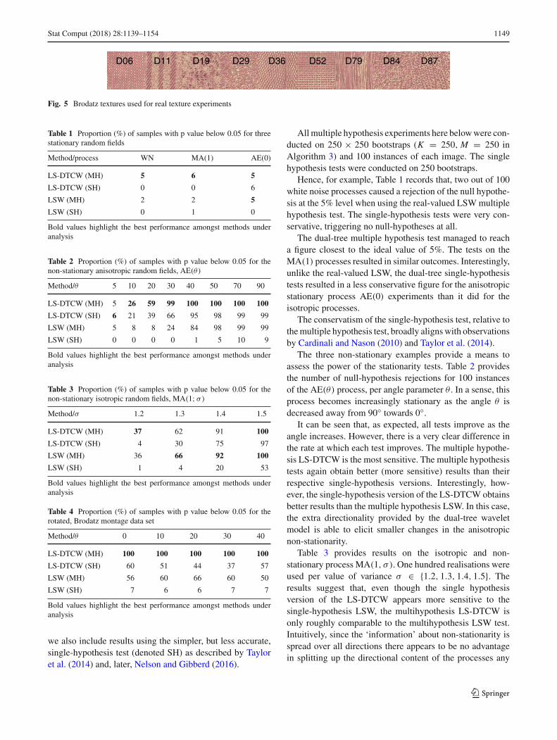
3. A montage of Brodatz textures: each half of the imagecomprised a different texture, selected from the Brodatztexture sub-catalogue: D06, D11, D19, D29, D36, D52,D79, D84, D87, cg. Fig. 5. The images were then rotatedby angles {0◦, 10◦, 20◦, 30◦, 40◦}.

Remark 4 Note that processes AE(θ) are stationary for θ =0 and non-stationary for any other value. The non-stationarityis due to the angular difference in the orientation of the tex-tures in the inner and outer regions.

Algorithm 3 Multi-hypothesis Stationarity detection, cf.Taylor et al. (2014)p = TESTSTAT(X)

Input: image XOutput: p-value p

Estimate observed local spectrum Sη = LWSE(X)

Compute observed statistic τ∗(η) = var(Sη

)

for k in 1 : K bootstraps doSimulate X k = LWSIM(X) with Alg. 2Estimate bootstrapped local spectrum Skη = LWSE(Xk)

Compute statistic τk(η) = var(Skη

)

for m in 1 : M bootstraps doSimulate X km = LWSIM(Xi ) with Alg. 2Est. bootstrapped spectrum Skmη = LWSE(Xkm)

Compute statistic τkm(η) = var(Skmη

)

Compute test statisticqk :=(M + 1)−1min

{1 + #{τk(η) ≤ τkm(η)}Mm=1

}η∈H

Compute test statisticq∗ :=(K + 1)−1min

{1 + #{τ∗(η) ≤ τk(η)}Kk=1

}η∈H

Compute p-value p := 1 + #{qk ≤ q∗}Kk=1

K + 1

4.3 Stationarity results

Wehere compare the locally stationarity (real-valued)wavelettest with that of the locally stationary dual-tree complexwavelet test. For completeness, in addition to the multiplehypothesis tests, denoted by MH in Tables 1, 2, 3 and 4,

123

Stat Comput (2018) 28:1139–1154 1149

D06 D11 D19 D29 D36 D52 D79 D84 D87

Fig. 5 Brodatz textures used for real texture experiments

Table 1 Proportion (%) of samples with p value below 0.05 for threestationary random fields

Method/process WN MA(1) AE(0)

LS-DTCW (MH) 5 6 5

LS-DTCW (SH) 0 0 6

LSW (MH) 2 2 5

LSW (SH) 0 1 0

Bold values highlight the best performance amongst methods underanalysis

Table 2 Proportion (%) of samples with p value below 0.05 for thenon-stationary anisotropic random fields, AE(θ)

Method/θ 5 10 20 30 40 50 70 90

LS-DTCW (MH) 5 26 59 99 100 100 100 100

LS-DTCW (SH) 6 21 39 66 95 98 99 99

LSW (MH) 5 8 8 24 84 98 99 99

LSW (SH) 0 0 0 0 1 5 10 9

Bold values highlight the best performance amongst methods underanalysis

Table 3 Proportion (%) of samples with p value below 0.05 for thenon-stationary isotropic random fields, MA(1; σ)

Method/σ 1.2 1.3 1.4 1.5

LS-DTCW (MH) 37 62 91 100

LS-DTCW (SH) 4 30 75 97

LSW (MH) 36 66 92 100

LSW (SH) 1 4 20 53

Bold values highlight the best performance amongst methods underanalysis

Table 4 Proportion (%) of samples with p value below 0.05 for therotated, Brodatz montage data set

Method/θ 0 10 20 30 40

LS-DTCW (MH) 100 100 100 100 100

LS-DTCW (SH) 60 51 44 37 57

LSW (MH) 56 60 66 60 50

LSW (SH) 7 6 6 7 7

Bold values highlight the best performance amongst methods underanalysis

we also include results using the simpler, but less accurate,single-hypothesis test (denoted SH) as described by Tayloret al. (2014) and, later, Nelson and Gibberd (2016).

Allmultiple hypothesis experiments here belowwere con-ducted on 250 × 250 bootstraps (K = 250, M = 250 inAlgorithm 3) and 100 instances of each image. The singlehypothesis tests were conducted on 250 bootstraps.

Hence, for example, Table 1 records that, two out of 100white noise processes caused a rejection of the null hypothe-sis at the 5% level when using the real-valued LSWmultiplehypothesis test. The single-hypothesis tests were very con-servative, triggering no null-hypotheses at all.

The dual-tree multiple hypothesis test managed to reacha figure closest to the ideal value of 5%. The tests on theMA(1) processes resulted in similar outcomes. Interestingly,unlike the real-valued LSW, the dual-tree single-hypothesistests resulted in a less conservative figure for the anisotropicstationary process AE(0) experiments than it did for theisotropic processes.

The conservatism of the single-hypothesis test, relative tothemultiple hypothesis test, broadly alignswith observationsby Cardinali and Nason (2010) and Taylor et al. (2014).

The three non-stationary examples provide a means toassess the power of the stationarity tests. Table 2 providesthe number of null-hypothesis rejections for 100 instancesof the AE(θ) process, per angle parameter θ . In a sense, thisprocess becomes increasingly stationary as the angle θ isdecreased away from 90◦ towards 0◦.

It can be seen that, as expected, all tests improve as theangle increases. However, there is a very clear difference inthe rate at which each test improves. The multiple hypothe-sis LS-DTCW is the most sensitive. The multiple hypothesistests again obtain better (more sensitive) results than theirrespective single-hypothesis versions. Interestingly, how-ever, the single-hypothesis version of the LS-DTCW obtainsbetter results than the multiple hypothesis LSW. In this case,the extra directionality provided by the dual-tree waveletmodel is able to elicit smaller changes in the anisotropicnon-stationarity.

Table 3 provides results on the isotropic and non-stationary process MA(1, σ ). One hundred realisations wereused per value of variance σ ∈ {1.2, 1.3, 1.4, 1.5}. Theresults suggest that, even though the single hypothesisversion of the LS-DTCW appears more sensitive to thesingle-hypothesis LSW, the multihypothesis LS-DTCW isonly roughly comparable to the multihypothesis LSW test.Intuitively, since the ‘information’ about non-stationarity isspread over all directions there appears to be no advantagein splitting up the directional content of the processes any

123

1150 Stat Comput (2018) 28:1139–1154

further than the three bands of the usual real-valued waveletdecomposition.

Finally, Table 4 shows the results from the Brodatz data.The percentage of null-hypothesis rejections are presentedover the data set of 72 montage images. Again, the multi-ple hypothesis tests detect more non-stationarities than thesingle hypothesis tests. The LS-DTCW correctly declaredall images to be non-stationary, irrespective of what anglethe data were rotated. The single-hypothesis LS-DTCW per-formed a little worse and much more inconsistently withrespect to angle than the multiple hypothesis LSW test.The single-hypothesis LSW test performed very poorly andonly managed to pick up 6 or 7% of the non-stationarities.This experiment lends some credence to the view that, aslong as some of the non-stationarity is distinguishable usingdirectional information, then a wavelet decomposition withgreater directionality may provide a more sensitive test.

5 Conclusions and further work

This work has focused on the case where the LSW spec-trum is smoothly varying in the Lipschitz sense. However,for complicated image scenes with multiple objects, anddistinct boundaries between those objects, a more realisticscenario would be to permit piecewise jumps in the under-lying spectrum. This alternative formalism, whereby thetransfer function W is assumed to have piecewise boundedvariation, has been explored for univariate, time-series LSWmodels in several other works such as Fryzlewicz and Nason(2006) and Nason and Stevens (2015) via the Haar–Fiszdevice. Extending this concept to the spatial and complexLSW model would provide a natural target for further work.

The main thrust of this work was to incorporate a waveletbasis into the existing LSW model which was even moreovercomplete than the existing undecimated basis. This ideacan be pushed further. Other bases are possible such asthe M-band extension of the dual-tree wavelets constructedby Chaux et al. (2006), wavelet packets schemes such asBayram and Selesnick (2008), andmixtures of wavelets suchas Nelson (2015). Although these constructions offer usefuladditional functionality, their statistically properties have yetto be explored. Placing such constructions in the LSW frame-work could provide an interestingmeans to extend the currenttheory and functionality.

Further work towards the non-stationarity detection appli-cation could also consider a more complete range ofanisotropy testing machinery such as that proposed by Mon-dal and Percival (2012) and Thon et al. (2015). It could alsoconsider incorporating the dual-tree complex framework intothe very recent multibasis approach of Cardinali and Nason(2016) which discovers a broader range of non-stationarybehaviours that is possible with only one basis on its own.

Acknowledgements This paper was primarily written by Dr. James D.B. Nelson who sadly passed away September 2016. At various pointsthroughout his life all the co-authors of this paperwere fortunate enoughto haveworkedwith James. It is an honour and privilege to complete thiswork on behalf of, and in the memory of such a humble and intelligentmember of our community.

Open Access This article is distributed under the terms of the CreativeCommons Attribution 4.0 International License (http://creativecommons.org/licenses/by/4.0/), which permits unrestricted use, distribution,and reproduction in any medium, provided you give appropriate creditto the original author(s) and the source, provide a link to the CreativeCommons license, and indicate if changes were made.

A Proofs

Lemma 2 Let w, W , and C be the transfer sequence, func-tion, and coefficients, respectively, from Definition 3. Then

|wη(t)|2 = |Wη(t/T )|2 + O(Cη/T ). (9)

Proof The result is easily obtained from Definition 1, prop-erty (1), viz.

supt

|wη(t) − Wη(t/T )| ≤ Cη

T

supt

|wη(t)| − |Wη(t/T )| ≤ Cη

T

|wη(t)| = |Wη(t/T )| + O(Cη/T )

|wη(t)|2 = |Wη(t/T )|2 + O(Cη/T )

= Sη(t/T ) + O(Cη/T ).

��

Lemma 3 Let S be the local wavelet spectrum of the LSWprocess X ∈ LSW(C). Then

Sη

(k + ·T

)= Sη

( ·T

)+ O(λη‖k/T ‖1).

Proof The proof follows that of Eckley et al. (2010) withoutany necessary adjustments. We include it here for com-pleteness. Using Definition 1, property (3), the triangularinequality, the square summability of the transfer function(Definition 1, property 2) and the boundedness of the Lip-schitz constants (Definition 1, property 4), respectively, wehave that

|Wη

(k + ·T

)− Wη

( ·T

)| ≤ λη‖k/T ‖1

|Wη

(k + ·T

)| − |Wη

( ·T

)| ≤ λη‖k/T ‖1

123

Stat Comput (2018) 28:1139–1154 1151

|Wη

(k + ·T

)| = |Wη

( ·T

)| + O

(λη‖k/T ‖1

)

|Wη

(k + ·T

)|2 = |Wη

( ·T

)|2+O

(λη‖k/T ‖1

).

��Theorem 1 (Convergence of auto-covariance) Let C andCT be, respectively, the local auto-covariance and auto-covariance of an LSW process {X (t)}t∈T ∈ LSW(C). Then

|CT (z, t) − C(z, t)|= O(T−1).

as T → ∞, uniformly in t ∈ Z2, and z ∈ T

2.

Proof Since X is zero mean,

CT (z, t) = E{X ([zT ])X ([zT ] + t)}= E

{ ∑

η,ν∈H

(w

ηξη ∗ ψη

)([zT ])(wνξν ∗ ψ

ν

)([zT ] + t)

},

where [·] denotes the integer part of · . The orthonormality ofthe increments gives

CT (z, t) =∑

η∈H

∑

k∈Z2

∣∣wη(k + [zT ])∣∣2 Ψη(k, t) ,

withΨη(k, t) := ψη(k)ψη(k−t). The remainder of the proof

now follows the same arguments as Eckley et al. (2010),namely:

|CT (z, t) − C(z, t)|=

∣∣∣∣∑

η∈H

∑

k∈Z2

|wη(k + [zT ])|2Ψη(k, t) −∑

η∈HSη(z)Ψη(t)

∣∣∣∣

=∣∣∣∣∑

η∈H

∑

k∈Z2

(|wη(k + [zT ])|2−Sη(k/T + z))Ψη(k, t)

−∑

η∈H

∑

k∈Z2

(Sη(k/T + z) − Sη(z)

)Ψη(k, t)

∣∣∣∣

≤∑

η∈H

∑

k∈Z2

∣∣Ψη(k, t)∣∣(∣∣|wη(k + [zT ]|2 − Sη(k/T + z)

∣∣

+ ∣∣Sη(k/T + z) − Sη(z)∣∣)

Lemmas 2 and 3 now yield

|CT (z, t) − C(z, t)| ≤∑

η∈H

∑

k∈Z2

∣∣Ψη(k, t)∣∣Cη + λη

∥∥k∥∥1

T,

and the result is obtained by invoking the boundedness prop-erties (1 and 4 from Definition 1) of the constants C and λ.

��

Theorem 2 (Periodogram bias) Let the LSW(C) processX : T �→ R, defined on the lattice T := [[1, T ]]2, haveperiodogram X∼

η :=∣∣∣X ∗ ψ

η

∣∣∣2, where {ψη}η∈H is a dis-

crete, undecimated, dual-tree complex wavelet basis and letA be the associated biasing matrix. Then

EX∼η =

∑

ν

AηνSν

( ·T

)+ O(T−1) (10)

Proof The proof follows the spirit of Eckley et al. (2010),but, here, special attention is required to take care of the factthat both the wavelet functions ψ and the transfer sequencesw are complex-valued, rather than real-valued. In addition,a slightly more ‘operator-theory’ flavour is applied to thefinal elements of the calculations whereby convolution prop-erties are exploited to circumvent the need for some tediouschanges of variables.

EX∼η = E|X ∗ ψ

ηrvert2

= E

∣∣∣∣∑

t∈TX (t)ψ

η(· − t)

∣∣∣∣2

= E

∣∣∣∣∑

t∈T

∑

ν∈H

∑

k∈Z2

wν(k)ξν(k)ψν(k − t)ψη(· − t)

∣∣∣∣2

=∑

ν∈H

∑

k∈Z2

|wν(k)|2∣∣∣∣∑

t∈Tψν(k − t)ψ

η(· − t)

∣∣∣∣2

=∑

ν∈H

∑

k∈Z2

|wν(k + ·)|2∣∣∣∣∑

t∈Tψν(k − t)ψ

η(−t)

∣∣∣∣2

=∑

ν∈H

∑

k∈Z2

|wν(k + ·)|2∣∣(ψν ∗ ψη)(k)

∣∣2,

where the fourth equality results from the orthonormality ofthe increment processes ξ . From Lemma 2, we now use thefact that

∣∣wν(k + ·)∣∣2 = Sν

(k + ·T

)+ O

(Cν

T

),

to write

EX∼η =

∑

ν∈H

∑

k∈Z2

(Sν

(k + ·T

)+O

(Cν

T

))∣∣(ψν ∗ψη)(k)

∣∣2.

Now, since∑

ν∈H Cν < ∞ and, since the∣∣(ψν ∗ψ

η)(k)∣∣2

is finite and bounded as a function of k (recall ψ has finitesupport), then

EX∼η =

∑

ν∈H

∑

k∈Z2

S

(k + ·T

)∣∣(ψν ∗ ψη)(k)

∣∣2 + O(T−1) .

123

1152 Stat Comput (2018) 28:1139–1154

From Lemma 3, we similarly use

S

(k + ·T

)= S

( ·T

)+ O

(λν‖k‖1

T

),

to get that

EX∼η =

∑

ν∈HS

( ·T

) ∑

k∈Z2

∣∣(ψν ∗ ψη)(k)

∣∣2 + O(T−1).

Finally, the following convolution property completes theproof.

∑

k∈Z2

|(ψν ∗ ψη)(k)|2 =

∑

k∈Z2

(ψν ∗ ψη)(k)(ψν ∗ ψ

η)(k)

=∑

k∈Z2

(ψη ∗ ψη)(k)(ψν ∗ ψ

ν )(k)

=∑

k∈Z2

Ψη(k)Ψν (k)

= 〈Ψη,Ψν〉= Aην.

��Lemma 1 (Bias is real) LetΨ be the ACW (Definition 2. Theentries of the biasing matrix (Definition 5) are positive, real,and symmetric.

Proof By construction, A is a Gram matrix. Hence, symme-try follows immediately. We then invoke Plancherel to writeAη,ν = ⟨

ψη ∗ ψη, ψν ∗ ψ

ν

⟩ = ⟨∣∣ψ∧η

∣∣2,∣∣ψ∧

ν

∣∣2⟩. ��Theorem 3 (Invertibility of the biasing matrix) Let the bias-ing matrix A′ associated with an appropriately chosenreal-valuedwaveletψ·;0 definedover [[1, T ]]benon-singular.Then, the biasing matrix A (Definition 5) associated withthe dual-tree wavelet (cf. Property 5 of Definition 1) ψ =ψ·;0 + iψ·;1 is non-singular with A = 2A′.

Proof We use the same arguments as the proof of Lemma1 and then note that the Fourier magnitudes of the real andimaginary parts of the dual-tree wavelets are identical bydesign:

Aη,ν = ⟨ψη ∗ ψ

η, ψν ∗ ψν

⟩

= ⟨∣∣ψ∧η

∣∣2,∣∣ψ∧

ν

∣∣2⟩

= ⟨∣∣ψ∧η;0

∣∣2 + ∣∣ψ∧η;1

∣∣2,∣∣ψ∧

ν;0∣∣2 + ∣∣ψ∧

ν;1∣∣2⟩

= 2⟨∣∣ψ∧

η;0∣∣2,

∣∣ψ∧ν;0

∣∣2⟩.

Unlike the brief proof in Nelson andGibberd (2016), we herejustify why the real and imaginary parts have the same filtercharacteristic, namely

∣∣ψ∧η;1

∣∣2 = ∣∣ψ∧η;0

∣∣2. The strategy is to

writeψ∧η;1 in terms of the filter sequence frequency responses

h1∧1 and h1∧0 . The filter relations in Eqs. (3) and (4) are thenused to write these in terms of h0∧1 and h0∧0 and hence strikean explicit comparison with respect to the filter response ofthe real wavelet ψ∧

η;0.Firstly, from the dual-tree wavelet filter properties (3) and

(4) and the dual-tree version of the recursions in Equation(2), namely:

ψ j;a =∑

k

ha0(· − 2k) ψ j−1(k), j > 0 (11)

ψ0;a = ha1, (12)

we have that:

ψ∧0;1(ω) = h1∧1 (ω) = 1√

2

∑

t

h11(t) e−iωt

= (−1)n−1 1√2

∑

t

h01(n − t − 1) e−iωt

= (−1)n−1e−i(n−1)ωh0∧1 (−ω). (13)

Likewise, we have that

h1∧0 (ω) = 1√2

∑

t

h10(t) e−iωt

= 1√2

∑

t

h00(n − t − 1) e−iωt

= e−i(n−1)ωh00(−ω). (14)

Now, from Equation (11), we have

ψ∧j;0(ω) = 2( j−1)/2 h0∧1 (2 jω)

j−1∏

�=0

h0∧0 (2�ω).

Similarly,

ψ∧j;1(ω) = 2( j−1)/2 h1∧1 (2 jω)

j−1∏

�=0

h1∧0 (2�ω).

Now, using (13) and (14) gives

ψ∧j;1(ω) = 2( j−1)/2(−1)n−1 e−i(n−1)2 jω h0∧1 (−2 jω)×

j−1∏

�=0

e−i(n−1)2�ω h00(−2�ω)

= z j 2( j−1)/2 h0∧1 (−2 jω)

j−1∏

�=0

h00(−2�ω),

123

Stat Comput (2018) 28:1139–1154 1153

with z j = (−1)n−1e−i(n−1)(2 j+1−1)ω. But the right-hand sidecan be expressed in terms of ψ∧

j;1(ω), viz.

ψ∧j;1(ω) = z jψ

∧j;0(−ω)

= z jψ∧∗j;0(ω).

Noting that |z j | = 1 completes the proof. ��Theorem 4 (Linear independence of ACW) Let the auto-correlation wavelet Ψ ′ associated with an appropriatelychosen real discrete wavelet function ψ·;0 defined over[[1, T ]] be linearly independent. Then, the auto-correlationwavelet Ψ associated with the dual-tree wavelet ψ = ψ·;0 +iψ·;1 is also linearly independent.

Proof This result holds courtesy of the equivalent resultin Theorem 3. However, we here provide an extra proofrestricted to the real scalars as an alternative means to estab-lish Corollary 1.

We have

∑

η∈HΔη(z)Ψη(t) = 0

⇒ �∑

η∈HΔη(z)Ψη(t) = 0

⇒∑

η∈HΔη(z)�

(ψη ∗ ψ∗

η

)(t) = 0

⇒∑

η∈HΔη(z)

(ψη;0 ∗ ψη;0 + ψη;1 ∗ ψη;1

) = 0

Now we note that ψη;1 ∗ ψη;1 = ψη;0 ∗ ψη;0 because convo-lution is commutative and ψ·;1 (and ψ·;1) are just translatedversions of ψ·;0 (and ψ·;0), respectively. Hence, we haveestablished that

∑

η∈HΔη(z)Ψη(t) = 0 ⇒

∑

η∈HΔη(z)Ψ

′η(t) = 0,

for all t ∈ Z2, z ∈ T

2. But we know that, since Ψ ′ is linearlyindependent we must therefore have that Δη(z) = 0. Hence,Ψ is also linearly independent. ��Corollary 1 (LWSuniqueness)TheLWS is uniquely defined,given the corresponding LSW(C) process.

Proof Similar to Nason et al. (2000) and Eckley et al. (2010),we follow a proof by contradiction and assume that the LWSis not uniquely defined. In which case, there exist two dif-ferent LWS sequences {S(1)

η (z)}z∈T2 and {S(2)η (z)}z∈T2 , say,

which are associated with the same process and hence giverise to the same local auto-correlation, namely

C(z, t) =∑

η∈HS(1)η (z)Ψη(t) =

∑

η∈HSη(z)

(2)Ψη(t),

for z ∈ T2, t ∈ Z

2. Defining

Δη(z) := S(1)η (z) − S(2)

η (z) ∈ R,

this would mean that

∑

η∈HΔη(z)Ψη(t) = 0. (15)

However, by Theorem 4, Ψ is linearly independent withrespect to real scalars and the only way that (15) could hold,therefore, is if Δη(z) = 0 which contradicts the originalassumption. ��Proposition 1 (LS-DTCW covariance inversion) Assumethat the debiasing matrix A is non-singular, then

Sη(z) =∑

ν

A−1η,ν

∑

t

C(z, t)Ψ ν (t).

Proof As in Nelson and Gibberd (2016) and Nason et al.(2000), we follow a proof by verification and then note thatA is both symmetric and, by Lemma 1, real.:

∑

ν

A−1η,ν

∑

t

∑

η′Sη′(z)Ψη′(t)Ψ

ν (t)

=∑

η′Sη′(z)

∑

ν

A−1η,ν

∑

t

Ψη′(t)Ψ ν (t)

=∑

η′Sη′(z)

∑

ν

A−1η,ν Aν,η′ =

∑

η′Sη′(z)δη,η′ = Sη(z).

��

References

Anantrasirichai, N., Achim, A., Bull, D.R., Kingsbury, N.: Atmosphericturbulence mitigation using complex wavelet-based fusion. IEEETrans. Image Process. 22(6), 2398–2408 (2013)

Bayram, I., Selesnick, I.W.: On the dual-tree complex wavelet packetandM-band transforms. IEEE Trans. Signal Process. 56(6), 2298–2310 (2008)

Cardinali, A., Nason, G.P.: Costationarity of locally stationary timeseries. J. Time Ser. Econom. 2(2), 1–33 (2010)

Cardinali, A., Nason, G.P.: Practical powerful wavelet packet tests forsecond-order stationarity. Appl. Comput. Harmon. Anal. (2016).https://doi.org/10.1016/j.acha.2016.06.006

Chaux, C., Duval, L., Pesquet, J.-C.: Image analysis using a dual-treeM-band wavelet transform. IEEE Trans. Image Process. 15(8),2397–2412 (2006)

Cho, H., Fryzlewicz, P.: Multiple change-point detection for high-dimensional time series via sparsified binary segmentation. J. R.Stat. Soc. B 77, 475–507 (2015)

Dahlhaus, R.: Fitting time series models to nonstationary processes.Ann. Stat. 25, 1–37 (1997)

Daubechies, I.: Ten Lectures on Wavelets. SIAM, Philadelphia (1992)Davison, A., Hinkley, D.: Bootstrap Methods and Their Application.

Cambridge University Press, Cambridge (1997)

123

1154 Stat Comput (2018) 28:1139–1154

Do,M.N., Vetterli, M.: Contourlets: a directional multiresolution imagerepresentation. In: IEEE International Conference on Image Pro-cessing, pp. 357–360 (2002)

Eckley, I.A., Nason, G.P.: LS2W: locally stationary wavelet fields in R.J. Stat. Softw. 43(3), 1–23 (2011)

Eckley, I.A., Nason, G.P., Treloar, R.L.: Locally stationary waveletfields with application to the modeling and analysis of image tex-ture. J. R. Stat. Soc. Ser. C (Appl. Stat.) 59(4), 595–616 (2010).https://doi.org/10.1111/j.1467-9876.2009.00721.x

Fryzlewicz, P.: Modelling and forecasting financial log-returns aslocally stationary wavelet processes. J. Appl. Stat. 32, 503–528(2005)

Fryzlewicz, P., Nason, G.P.: Haar-fisz estimation of evolutionarywavelet spectra. J. R. Stat. Soc. Ser. B (Stat. Methodol.) 68, 611–634 (2006)

Gibberd, A.J., Nelson, J.D.B.: Regularised estimation of 2d-locallystationary wavelet processes. In: 2016 IEEE Statistical SignalProcessing Workshop (SSP) (2016). https://doi.org/10.1109/ssp.2016.7551838

Hill, P.R., Anantrasirichai, N., Achim, A., Al-Mualla, M.E., Bull, D.R.:Undecimated dual-tree complex wavelet transforms. Signal Pro-cess. Image Commun. 35, 61–70 (2015)

Hubel, D.H., Wiesel, T.N.: Receptive fields, binocular interaction andfunctional architecture in the cats visual cortex. J. Physiol. 160(1),106–154.2 (1962)

Hussain, M., Chen, D., Cheng, A., Wei, H., Stanley, D.: Changedetection from remotely sensed images: from pixel-based toobject-based approaches. ISPRS J. Photogram. Remote Sens. 80,91–106 (2013)

Killick, R., Eckley, I.A., Jonathan, P.: A wavelet-based approach fordetecting changes in second order structure within nonstationarytime series. Electron. J. Stat. 7, 1167–1183 (2013)

Kingsbury, N.G.: Complex wavelets for shift invariant analysis and fil-tering of signals. J. Appl. Comput. Harmon. Anal. 10(3), 234–253(2001)

Kingsbury, N.G.: Design of q-shift complex wavelets for image pro-cessing using frequency domain energy minimisation. In: IEEEInternational Conference on Image Processing (2003)

Knight, M.I., Nunes, M.A., Nason, G.P.: Spectral estimation for locallystationary time series with missing observations. Stat. Comput.22(4), 877–895 (2012)

Mondal, D., Percival, D.B.:Wavelet variance analysis for random fieldson a regular lattice. IEEE Trans. Image Process. 21(2), 537–549(2012)

Nadaraya, E.: On estimating regression. Theory Probab. Appl. 9(1),141–142 (2016)

Nason, G.P.: A test for second-order stationarity and approximate confi-dence intervals for localized autocovariances for locally stationarytime series. J. R. Stat. Soc. Ser. B (Stat. Methodol.) 75, 879–904(2013)

Nason, G., Stevens, K.: Bayesian wavelet shrinkage of the Haar-Fisztransformed wavelet periodogram. PLoS One 10(9), e0137662(2015). https://doi.org/10.1371/journal.pone.0137662

Nason, G.P., von Sachs, R., Kroisandt, G.: Wavelet processes and adap-tive estimation of the evolutionary wavelet spectrum. J. R. Stat.Soc. Ser. B (Stat. Methodol.) 62, 271–292 (2000)

Nelson, J.D.B.: Enhanced B-wavelets via mixed, composite packets.IEEE Trans. Signal Process. 63(12), 3191–3203 (2015)

Nelson, J.D.B., Gibberd, A.J.: Introducing the locally stationary dual-tree complex wavelet model. In: IEEE International Conferenceon Image Processing (2016)

Nelson, J.D.B., Kingsbury, N.G.: Fractal dimension based sand ripplesuppression for mine huntingwith sidescan sonar. In: InternationalConference on Synthetic Aperture Sonar and Synthetic ApertureRadar (2010)

Nelson, J.D.B., Kingsbury, N.G.: Fractal dimension, wavelet shrinkageand anomaly detection for mine hunting. IET Signal Process. 6(5),484–493 (2012)

Nelson, J.D.B., Nafornita, C., Isar, A.: Semi-local scaling exponentestimation with box-penalty constraints and total-variation regu-larization. IEEE Trans. Image Process. 25(7), 3167–3181 (2016)

Ng, J., Bharath, A.A., Zhaoping, L.: A survey of architecture and func-tion of the primary visual cortex (V1). EURASIP J. Adv. SignalProcess. 2007(1), 097961 (2006). https://doi.org/10.1155/2007/97961

Nunes, M.A., Taylor, S., Eckley, I.A.: A multiscale test of spatial sta-tionarity for textured images in R. R J. 6, 20–30 (2014)

Portilla, J., Simoncelli, E.P.: A parametric texture model based on jointstatistics of complex wavelet coefficients. Int. J. Comput. Vis. 40,49–70 (2000)

Raj, R.G., Bovik, A.C., Geisler, W.S.: Non-stationarity detection innatural images. In: IEEE International Conference on Image Pro-cessing (2007)

Sanderson, J., Fryzlewicz, P., Jones, M.W.: Estimating linear depen-dence between nonstationary time series using the locally station-ary wavelet model. Biometrika 97(2), 435–446 (2010)

Selesnick, I.W., Baraniuk, R.G., Kingsbury, N.G.: The dual-tree com-plexwavelet transform. IEEESignal Process.Mag.22(6), 123–151(2005)

Starck, J.-L., Cands, E.J., Donoho, D.L.: The curvelet transform forimage denoising. IEEE Trans. Image Process. 11(6), 670–684(2002)

Taylor, S., Eckley, I.A., Nunes, M.A.: A test of stationarity for texturedimages. Technometrics 56, 291–301 (2014)

Taylor, S., Eckley, I.A., Nunes, M.A.: Multivariate locally stationary 2dwavelet processes with application to colour texture analysis. Stat.Comput. (2017)

Thon, K., Geilhufe, M., Percival, D.B.: A multiscale wavelet-based testfor isotropy of random fields on a regular lattice. IEEE Trans.Image Process. 24(2), 694–708 (2015)

Unser,M., Sage,D.,VanDeVille,D.:Multiresolutionmonogenic signalanalysis using the Riesz–Laplace wavelet transform. IEEE Trans.Image Process. 18(11), 2402–2418 (2009)

van Bellegem, S., von Sachs, R.: Locally adaptive estimation of evolu-tionary wavelet spectra. Ann. Stat. 36, 1879–1024 (2008)

von Sachs, R., Nason, G. P., Kroisandt, G.: Spectral representation andestimation for locally-stationary wavelet processes. In: Dubuc, S.(eds.) CRM Proceedings and Lecture Notes, vol. 18, pp. 381–397(1998)

Watson, G.: Smooth regression analysis. Indian J. Stat. 26, 359–372(1964)

Zhang, G., Kingsbury, N.: Variational Bayesian image restoration withgroup-sparse modeling of wavelet coefficients. Digit. Signal Pro-cess. (Special Issue in Honour of William J. (Bill) Fitzgerald) 47,157–168 (2015)

123