Embed Size (px)
Citation preview

Lecture 13The language SAT
Cook-Levin: SAT is NP-Complete.
Outline of the proof to Cook-Levin theorem.
Additional NP-Complete problemsby chains of reductions.
Slides modified by Benny Chor, based on original slides by Maurice Herlihy, Brown University. – p.1

Lecture 13The language SAT
Cook-Levin: SAT is NP-Complete.
Outline of the proof to Cook-Levin theorem.
Additional NP-Complete problemsby chains of reductions.
Slides modified by Benny Chor, based on original slides by Maurice Herlihy, Brown University. – p.1
Lecture 13The language SAT
Cook-Levin: SAT is NP-Complete.
Outline of the proof to Cook-Levin theorem.
Additional NP-Complete problemsby chains of reductions.
Slides modified by Benny Chor, based on original slides by Maurice Herlihy, Brown University. – p.1
Lecture 13The language SAT
Cook-Levin: SAT is NP-Complete.
Outline of the proof to Cook-Levin theorem.
Additional NP-Complete problemsby chains of reductions.
Slides modified by Benny Chor, based on original slides by Maurice Herlihy, Brown University. – p.1

Lecture 13The language SAT
Cook-Levin: SAT is NP-Complete.
Outline of the proof to Cook-Levin theorem.
Additional NP-Complete problemsby chains of reductions.
Slides modified by Benny Chor, based on original slides by Maurice Herlihy, Brown University. – p.1

NP-Completeness (reminder)
A language B is NP-complete if it satisfies
B ∈ NP , and
For every A in NP, A ≤P B
Slides modified by Benny Chor, based on original slides by Maurice Herlihy, Brown University. – p.2
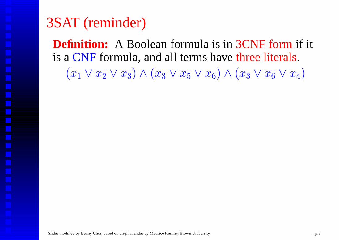
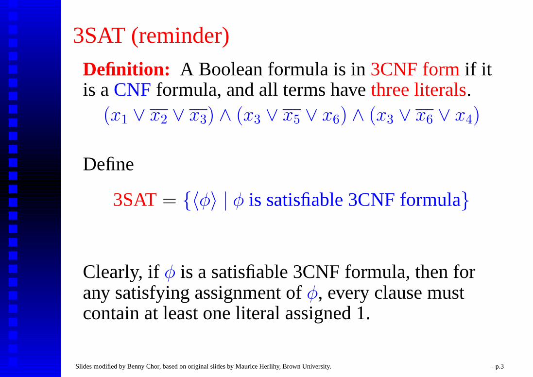
3SAT (reminder)
Definition: A Boolean formula is in 3CNF form if itis a CNF formula, and all terms have three literals.
(x1 ∨ x2 ∨ x3) ∧ (x3 ∨ x5 ∨ x6) ∧ (x3 ∨ x6 ∨ x4)
Define
3SAT = {〈φ〉 | φ is satisfiable 3CNF formula}
Clearly, if φ is a satisfiable 3CNF formula, then forany satisfying assignment of φ, every clause mustcontain at least one literal assigned 1.
Slides modified by Benny Chor, based on original slides by Maurice Herlihy, Brown University. – p.3

The Language SAT
Definition: A Boolean formula is in conjunctivenormal form (CNF) if it consists of terms, connectedwith ∧s.
For example(x1 ∨ x2 ∨ x3 ∨ x4) ∧ (x3 ∨ x5 ∨ x6) ∧ (x3 ∨ x6)
Definition:SAT = {〈φ〉 | φ is satisfiable CNF formula}
Slides modified by Benny Chor, based on original slides by Maurice Herlihy, Brown University. – p.4

Strategy
Once we have one structured NP-completeproblem, we can generate more by poly-timereductions.
Getting the first one requires some work.
Slides modified by Benny Chor, based on original slides by Maurice Herlihy, Brown University. – p.5

Strategy
Once we have one structured NP-completeproblem, we can generate more by poly-timereductions.
Getting the first one requires some work.
Slides modified by Benny Chor, based on original slides by Maurice Herlihy, Brown University. – p.5

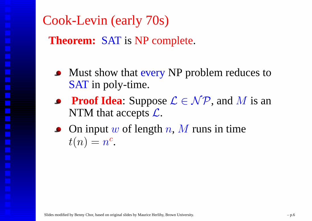
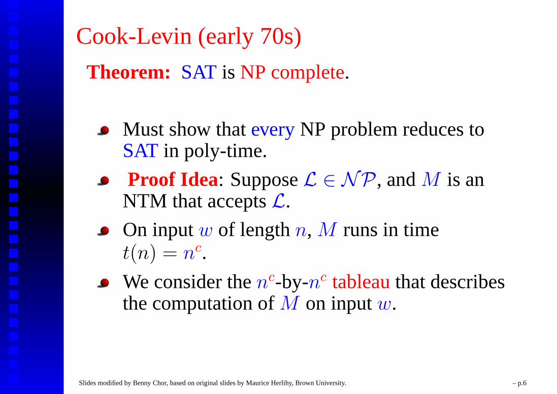
Cook-Levin (early 70s)
Theorem: SAT is NP complete.
Must show that every NP problem reduces toSAT in poly-time.
Proof Idea: Suppose L ∈ NP , and M is anNTM that accepts L.
On input w of length n, M runs in timet(n) = nc.
We consider the nc-by-nc tableau that describesthe computation of M on input w.
Slides modified by Benny Chor, based on original slides by Maurice Herlihy, Brown University. – p.6

The Tableau
cell[1,1]
cell[1,t(n)]
q 0 0 10 0 . . .1 2 3 . . . t(n)
0 00
1
Slides modified by Benny Chor, based on original slides by Maurice Herlihy, Brown University. – p.7

The Tableau
cell[1,1]
cell[1,t(n)]
q 0 0 10 0 . . .1 2 3 . . . t(n)
0 00
1
Row 1 in tableau represents initial configurationof M on input w.
Row i in tableau represents i-th configuration in acomputation of M on input w.
Slides modified by Benny Chor, based on original slides by Maurice Herlihy, Brown University. – p.8
A Formula Simulating the Tableau
We construct a Boolean CNF formula φw that“mimics” the tableau.
Given the string w, it takes O(n2c) steps toconstruct φw.
The following property holds:φw ∈ SAT iff M accepts w.
So the mapping w 7→ φw is a poly time reductionfrom L to SAT , establishing L ≤P SAT .
We still got a few small details to take care off...
Slides modified by Benny Chor, based on original slides by Maurice Herlihy, Brown University. – p.9

Details of Formula (Partial List)
We construct a Boolean CNF formula φw that“mimics” the tableau:
φw uses Boolean variables of three types.bi,j,σ is true iff the j-th cell in i-thconfiguration contains the letter σ ∈ Γ.si,q is true iff in i-th configuration, M is instate q ∈ Q.hi,j is true iff in i-th configuration M , has ishead in cell j on tape.
The formula φw consists of four parts:φw = φunique(M) ∧ φstart(w) ∧ φaccept(M) ∧
φcompute(M)
Slides modified by Benny Chor, based on original slides by Maurice Herlihy, Brown University. – p.10

Details of Formula (Partial List)
We construct a Boolean CNF formula φw that“mimics” the tableau:
φw uses Boolean variables of three types.
bi,j,σ is true iff the j-th cell in i-thconfiguration contains the letter σ ∈ Γ.si,q is true iff in i-th configuration, M is instate q ∈ Q.hi,j is true iff in i-th configuration M , has ishead in cell j on tape.
The formula φw consists of four parts:φw = φunique(M) ∧ φstart(w) ∧ φaccept(M) ∧
φcompute(M)
Slides modified by Benny Chor, based on original slides by Maurice Herlihy, Brown University. – p.10

Details of Formula (Partial List)
We construct a Boolean CNF formula φw that“mimics” the tableau:
φw uses Boolean variables of three types.bi,j,σ is true iff the j-th cell in i-thconfiguration contains the letter σ ∈ Γ.
si,q is true iff in i-th configuration, M is instate q ∈ Q.hi,j is true iff in i-th configuration M , has ishead in cell j on tape.
The formula φw consists of four parts:φw = φunique(M) ∧ φstart(w) ∧ φaccept(M) ∧
φcompute(M)
Slides modified by Benny Chor, based on original slides by Maurice Herlihy, Brown University. – p.10

Details of Formula (Partial List)
We construct a Boolean CNF formula φw that“mimics” the tableau:
φw uses Boolean variables of three types.bi,j,σ is true iff the j-th cell in i-thconfiguration contains the letter σ ∈ Γ.si,q is true iff in i-th configuration, M is instate q ∈ Q.
hi,j is true iff in i-th configuration M , has ishead in cell j on tape.
The formula φw consists of four parts:φw = φunique(M) ∧ φstart(w) ∧ φaccept(M) ∧
φcompute(M)
Slides modified by Benny Chor, based on original slides by Maurice Herlihy, Brown University. – p.10

Details of Formula (Partial List)
We construct a Boolean CNF formula φw that“mimics” the tableau:
φw uses Boolean variables of three types.bi,j,σ is true iff the j-th cell in i-thconfiguration contains the letter σ ∈ Γ.si,q is true iff in i-th configuration, M is instate q ∈ Q.hi,j is true iff in i-th configuration M , has ishead in cell j on tape.
The formula φw consists of four parts:φw = φunique(M) ∧ φstart(w) ∧ φaccept(M) ∧
φcompute(M)
Slides modified by Benny Chor, based on original slides by Maurice Herlihy, Brown University. – p.10

Details of Formula (Partial List)
We construct a Boolean CNF formula φw that“mimics” the tableau:
φw uses Boolean variables of three types.bi,j,σ is true iff the j-th cell in i-thconfiguration contains the letter σ ∈ Γ.si,q is true iff in i-th configuration, M is instate q ∈ Q.hi,j is true iff in i-th configuration M , has ishead in cell j on tape.
The formula φw consists of four parts:φw = φunique(M) ∧ φstart(w) ∧ φaccept(M) ∧
φcompute(M)
Slides modified by Benny Chor, based on original slides by Maurice Herlihy, Brown University. – p.10
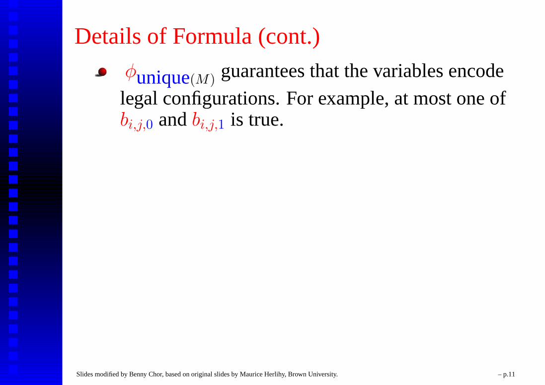
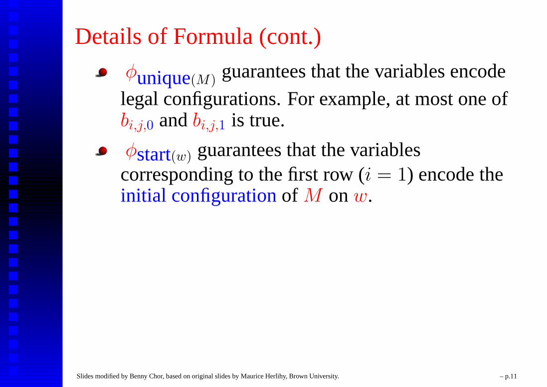
Details of Formula (cont.)
φunique(M) guarantees that the variables encode
legal configurations. For example, at most one ofbi,j,0 and bi,j,1 is true.
φstart(w) guarantees that the variablescorresponding to the first row (i = 1) encode theinitial configuration of M on w.
φaccept(M) guarantees that M reached anaccepting configuration.
φcompute(M) guarantees that the configurationdescribed by the i + 1-st row is a legal successionof the configuration described by the i-th row.
Slides modified by Benny Chor, based on original slides by Maurice Herlihy, Brown University. – p.11

Details of Formula (cont.)
φcompute(M) is the “heart” of φw. To constructit, employ locality of computations.
To determine contents of tableau entry (i, j) (cellj in configuration i), only the contents of threetableau entries (from configuration i− 1),(i− 1, j − 1), (i− 1, j), (i− 1, j + 1), and M ’stable, are needed.
If head not in area, nothing changes. And and if itis, changes are local and determined using M .
0 00
1
Slides modified by Benny Chor, based on original slides by Maurice Herlihy, Brown University. – p.12

The Tableau in Perspective
cell[1,1]
cell[1,t(n)]
q 0 0 10 0 . . .1 2 3 . . . t(n)
0 00
1
Slides modified by Benny Chor, based on original slides by Maurice Herlihy, Brown University. – p.13

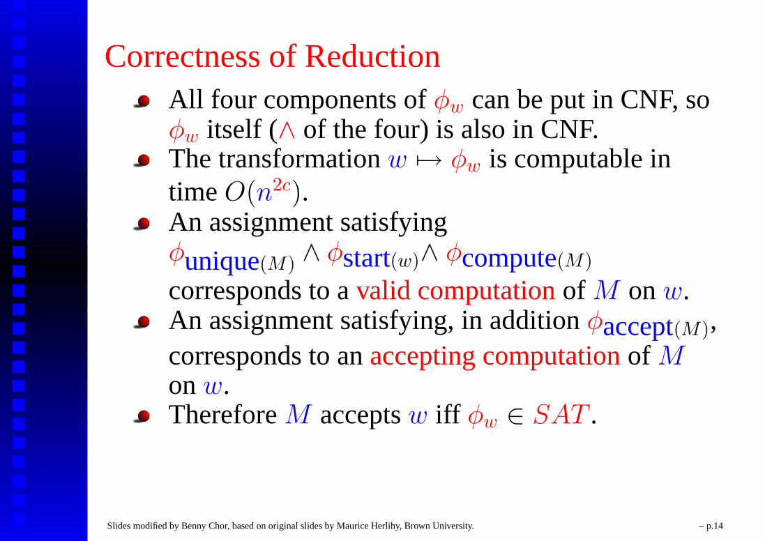
Correctness of ReductionAll four components of φw can be put in CNF, soφw itself (∧ of the four) is also in CNF.
The transformation w 7→ φw is computable intime O(n2c).An assignment satisfyingφunique(M) ∧ φstart(w)∧ φcompute(M)
corresponds to a valid computation of M on w.An assignment satisfying, in addition φaccept(M),corresponds to an accepting computation of Mon w.Therefore M accepts w iff φw ∈ SAT .
For complete details, consult Sipser or take theComplexity course. ♣
Slides modified by Benny Chor, based on original slides by Maurice Herlihy, Brown University. – p.14

Correctness of ReductionAll four components of φw can be put in CNF, soφw itself (∧ of the four) is also in CNF.The transformation w 7→ φw is computable intime O(n2c).
An assignment satisfyingφunique(M) ∧ φstart(w)∧ φcompute(M)
corresponds to a valid computation of M on w.An assignment satisfying, in addition φaccept(M),corresponds to an accepting computation of Mon w.Therefore M accepts w iff φw ∈ SAT .
For complete details, consult Sipser or take theComplexity course. ♣
Slides modified by Benny Chor, based on original slides by Maurice Herlihy, Brown University. – p.14

Correctness of ReductionAll four components of φw can be put in CNF, soφw itself (∧ of the four) is also in CNF.The transformation w 7→ φw is computable intime O(n2c).An assignment satisfyingφunique(M) ∧ φstart(w)∧ φcompute(M)
corresponds to a valid computation of M on w.
An assignment satisfying, in addition φaccept(M),corresponds to an accepting computation of Mon w.Therefore M accepts w iff φw ∈ SAT .
For complete details, consult Sipser or take theComplexity course. ♣
Slides modified by Benny Chor, based on original slides by Maurice Herlihy, Brown University. – p.14

Correctness of ReductionAll four components of φw can be put in CNF, soφw itself (∧ of the four) is also in CNF.The transformation w 7→ φw is computable intime O(n2c).An assignment satisfyingφunique(M) ∧ φstart(w)∧ φcompute(M)
corresponds to a valid computation of M on w.An assignment satisfying, in addition φaccept(M),corresponds to an accepting computation of Mon w.
Therefore M accepts w iff φw ∈ SAT .
For complete details, consult Sipser or take theComplexity course. ♣
Slides modified by Benny Chor, based on original slides by Maurice Herlihy, Brown University. – p.14

Correctness of ReductionAll four components of φw can be put in CNF, soφw itself (∧ of the four) is also in CNF.The transformation w 7→ φw is computable intime O(n2c).An assignment satisfyingφunique(M) ∧ φstart(w)∧ φcompute(M)
corresponds to a valid computation of M on w.An assignment satisfying, in addition φaccept(M),corresponds to an accepting computation of Mon w.Therefore M accepts w iff φw ∈ SAT .
For complete details, consult Sipser or take theComplexity course. ♣
Slides modified by Benny Chor, based on original slides by Maurice Herlihy, Brown University. – p.14

Strategy
We have seen that SAT is NP-complete.
We now reduce SAT to 3SAT.
And then will reduce 3SAT to a bunch of otherproblems in NP.
In class and recitation will give in detail just afew examples.
Full list contains hundreds or thousands of knownNP-complete problems (from combinatorics,operation research, VLSI design, computationalgeometry, bioinformatics, . . . ).
NP-completeness of new and of old problems isstill established these days.
Slides modified by Benny Chor, based on original slides by Maurice Herlihy, Brown University. – p.15

SAT and 3SATRecallSAT = {〈φ〉 | φ is a satisfiable CNF formula}
3SAT = {〈φ〉 | φ is satisfiable 3CNF formula}
The reduction maps CNF formulae to 3CNF ones“clause by clause”. A clause with ` literals is mappedto ` clauses, built on the original literals together with`− 1 new ones.
For example:
(x1 ∨ x2 ∨ x3 ∨ x4 ∨ x8)7−→(x1 ∨ y1) ∧ (y1 ∨ x2 ∨ y2) ∧ (y2 ∨ x3 ∨ y3) ∧(y3 ∨ x4∨y4) ∧ (y4 ∨ x8)
Slides modified by Benny Chor, based on original slides by Maurice Herlihy, Brown University. – p.16

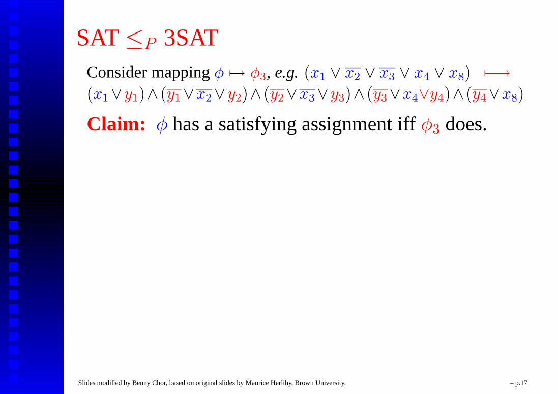
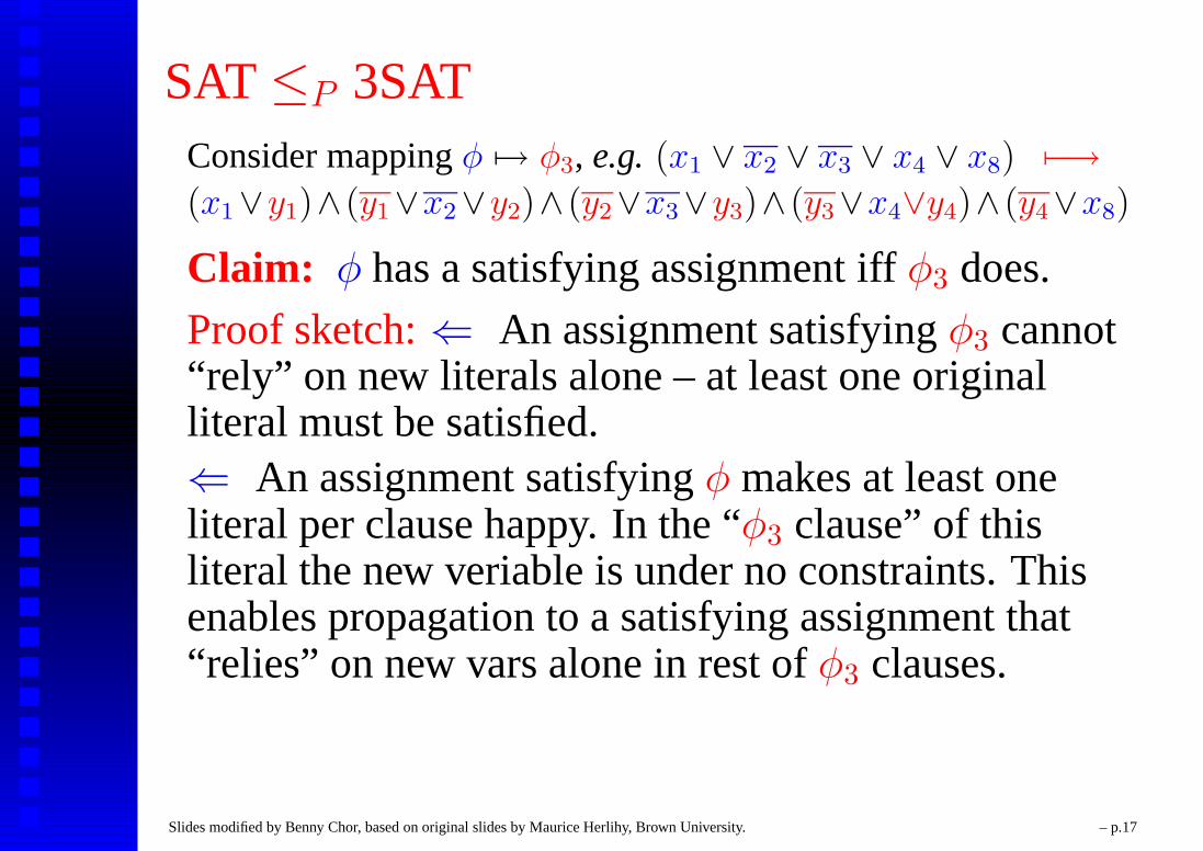
SAT ≤P 3SATConsider mapping φ 7→ φ3, e.g. (x1 ∨ x2 ∨ x3 ∨ x4 ∨ x8) 7−→(x1∨y1)∧ (y1∨x2∨y2)∧ (y2∨x3∨y3)∧ (y3∨x4∨y4)∧ (y4∨x8)
Claim: φ has a satisfying assignment iff φ3 does.
Proof sketch: ⇐ An assignment satisfying φ3 cannot“rely” on new literals alone – at least one originalliteral must be satisfied.⇐ An assignment satisfying φ makes at least oneliteral per clause happy. In the “φ3 clause” of thisliteral the new veriable is under no constraints. Thisenables propagation to a satisfying assignment that“relies” on new vars alone in rest of φ3 clauses.
This establishes validity of the reduction. Since it is inpolynomial time (why?), we get SAT ≤P 3SAT. ♣.
Slides modified by Benny Chor, based on original slides by Maurice Herlihy, Brown University. – p.17

SAT ≤P 3SATConsider mapping φ 7→ φ3, e.g. (x1 ∨ x2 ∨ x3 ∨ x4 ∨ x8) 7−→(x1∨y1)∧ (y1∨x2∨y2)∧ (y2∨x3∨y3)∧ (y3∨x4∨y4)∧ (y4∨x8)
Claim: φ has a satisfying assignment iff φ3 does.
Proof sketch: ⇐ An assignment satisfying φ3 cannot“rely” on new literals alone – at least one originalliteral must be satisfied.
⇐ An assignment satisfying φ makes at least oneliteral per clause happy. In the “φ3 clause” of thisliteral the new veriable is under no constraints. Thisenables propagation to a satisfying assignment that“relies” on new vars alone in rest of φ3 clauses.
This establishes validity of the reduction. Since it is inpolynomial time (why?), we get SAT ≤P 3SAT. ♣.
Slides modified by Benny Chor, based on original slides by Maurice Herlihy, Brown University. – p.17
SAT ≤P 3SATConsider mapping φ 7→ φ3, e.g. (x1 ∨ x2 ∨ x3 ∨ x4 ∨ x8) 7−→(x1∨y1)∧ (y1∨x2∨y2)∧ (y2∨x3∨y3)∧ (y3∨x4∨y4)∧ (y4∨x8)
Claim: φ has a satisfying assignment iff φ3 does.
Proof sketch: ⇐ An assignment satisfying φ3 cannot“rely” on new literals alone – at least one originalliteral must be satisfied.⇐ An assignment satisfying φ makes at least oneliteral per clause happy. In the “φ3 clause” of thisliteral the new veriable is under no constraints. Thisenables propagation to a satisfying assignment that“relies” on new vars alone in rest of φ3 clauses.
This establishes validity of the reduction. Since it is inpolynomial time (why?), we get SAT ≤P 3SAT. ♣.
Slides modified by Benny Chor, based on original slides by Maurice Herlihy, Brown University. – p.17

SAT ≤P 3SATConsider mapping φ 7→ φ3, e.g. (x1 ∨ x2 ∨ x3 ∨ x4 ∨ x8) 7−→(x1∨y1)∧ (y1∨x2∨y2)∧ (y2∨x3∨y3)∧ (y3∨x4∨y4)∧ (y4∨x8)
Claim: φ has a satisfying assignment iff φ3 does.
Proof sketch: ⇐ An assignment satisfying φ3 cannot“rely” on new literals alone – at least one originalliteral must be satisfied.⇐ An assignment satisfying φ makes at least oneliteral per clause happy. In the “φ3 clause” of thisliteral the new veriable is under no constraints. Thisenables propagation to a satisfying assignment that“relies” on new vars alone in rest of φ3 clauses.
This establishes validity of the reduction. Since it is inpolynomial time (why?), we get SAT ≤P 3SAT. ♣.
Slides modified by Benny Chor, based on original slides by Maurice Herlihy, Brown University. – p.17

3SAT – Cousins and CambriansWe now know that SAT ≤P 3SAT. Since SAT isNP-complete and 3SAT∈ NP, this proves that 3SAT isitself NP-complete.
What about the 3SAT ≤P SAT direction?
We now want to examine what happens if we furtherreduce the number of literals per clause in CNFformulae.
Definition: A Boolean formula is in 2CNF if it is aCNF formula, and all terms have at most two literals.For example
(x1 ∨ x2) ∧ (x5 ∨ x6) ∧ (x6 ∨ x4)
Slides modified by Benny Chor, based on original slides by Maurice Herlihy, Brown University. – p.18

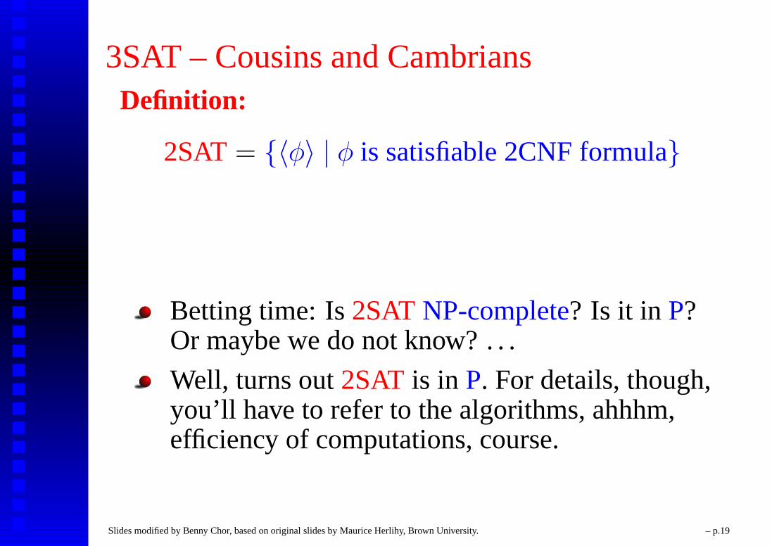
3SAT – Cousins and CambriansDefinition:
2SAT = {〈φ〉 | φ is satisfiable 2CNF formula}
Betting time: Is 2SAT NP-complete? Is it in P?Or maybe we do not know? . . .
Well, turns out 2SAT is in P. For details, though,you’ll have to refer to the algorithms, ahhhm,efficiency of computations, course.
Slides modified by Benny Chor, based on original slides by Maurice Herlihy, Brown University. – p.19

Chains of Reductions: NPC Problems
SAT
IntegerProg 3SAT
Clique
IndepSet
VertexCover
SetCover
3ExactCover
Knapsack
Scheduling
3Color HamPath
HamCircuit
TSP
Slides modified by Benny Chor, based on original slides by Maurice Herlihy, Brown University. – p.20

Hamiltonian Path (reminder)
HAMPATH = {〈G, s, t〉 | G has Hamiltonian pathfrom s to t}
Hamiltonian path in directed G visits each node once.
Slides modified by Benny Chor, based on original slides by Maurice Herlihy, Brown University. – p.21
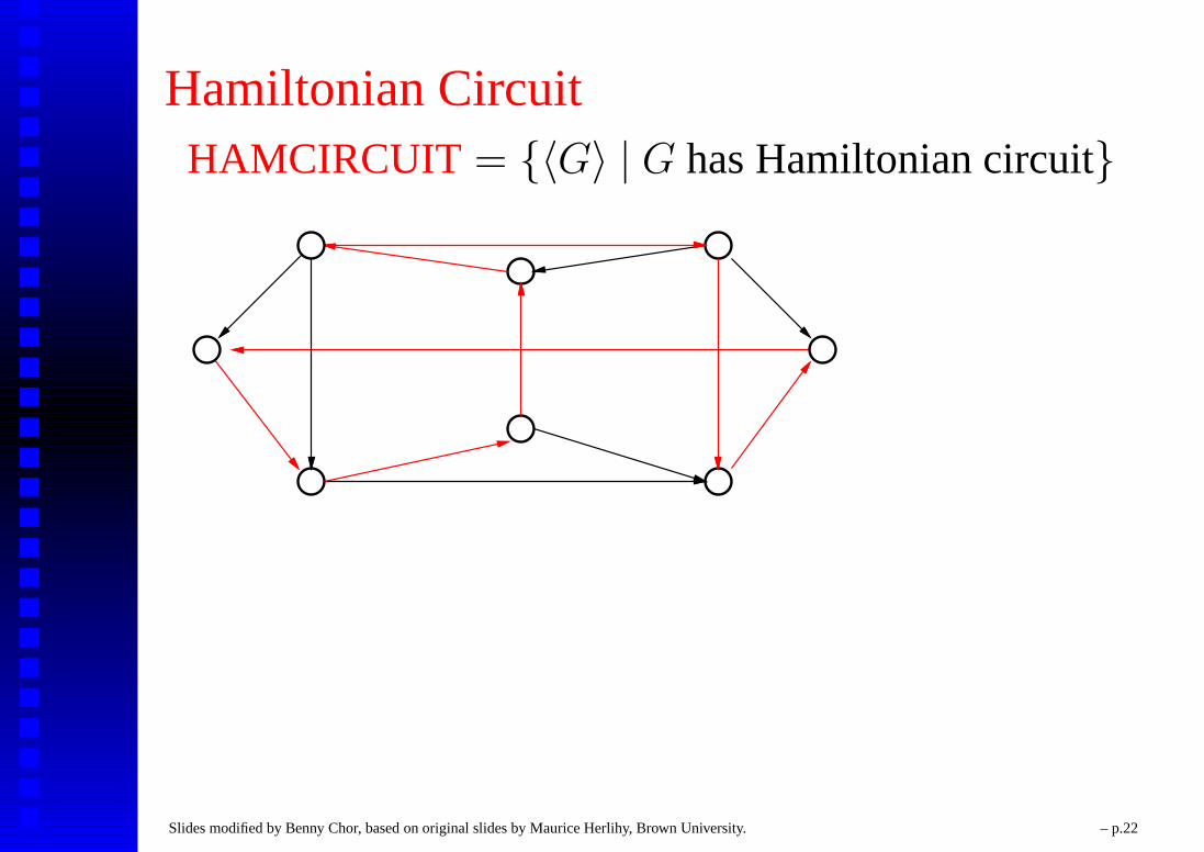
Hamiltonian CircuitHAMCIRCUIT = {〈G〉 | G has Hamiltonian circuit}
Slides modified by Benny Chor, based on original slides by Maurice Herlihy, Brown University. – p.22

Hamiltonian CircuitHAMCIRCUIT = {〈G〉 | G has Hamiltonian circuit}
Slides modified by Benny Chor, based on original slides by Maurice Herlihy, Brown University. – p.22

ReductionTheorem: HAMPATH is polynomial-time reducibleto HAMCIRCUIT ,
HAMPATH ≤P HAMCIRCUIT .
Slides modified by Benny Chor, based on original slides by Maurice Herlihy, Brown University. – p.23
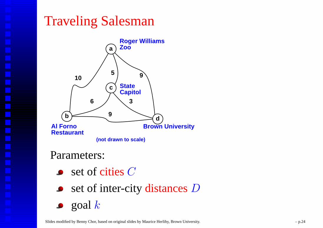
Traveling Salesman
10 9
36
9
a
b
c
d
5
Roger WilliamsZoo
Brown UniversityAl FornoRestaurant
StateCapitol
(not drawn to scale)
Parameters:
set of cities C
set of inter-city distances D
goal k
Slides modified by Benny Chor, based on original slides by Maurice Herlihy, Brown University. – p.24
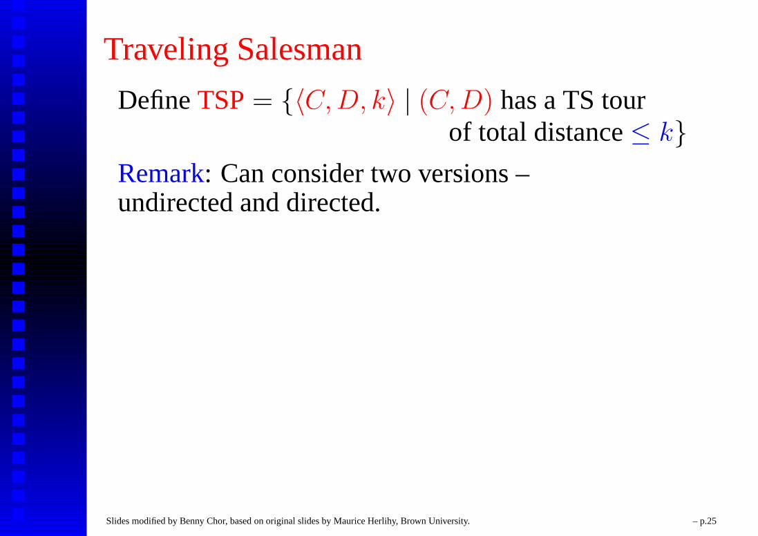
Traveling Salesman
Define TSP = {〈C,D, k〉 | (C,D) has a TS tourof total distance ≤ k}
Remark: Can consider two versions –undirected and directed.
RecallHAMCIRCUIT = {〈G〉 | G has Hamiltonian circuit}
Theorem: HAMCIRCUIT is polynomial-timereducible to TSP,
HAMCIRCUIT ≤P TSP .
Slides modified by Benny Chor, based on original slides by Maurice Herlihy, Brown University. – p.25

HAMCIRCUIT≤P TSP
The reduction: Given a directed graph G = (V,E) weconstruct a directed traveling salesman instance.
The cities are identical to the nodes of theoriginal graph, C = V .
The distance of going from v1 to v2 is 1 if(v1, v2) ∈ E, and 2 otherwise.
The bound on the total distance of a tour isk = |V |.
Slides modified by Benny Chor, based on original slides by Maurice Herlihy, Brown University. – p.26

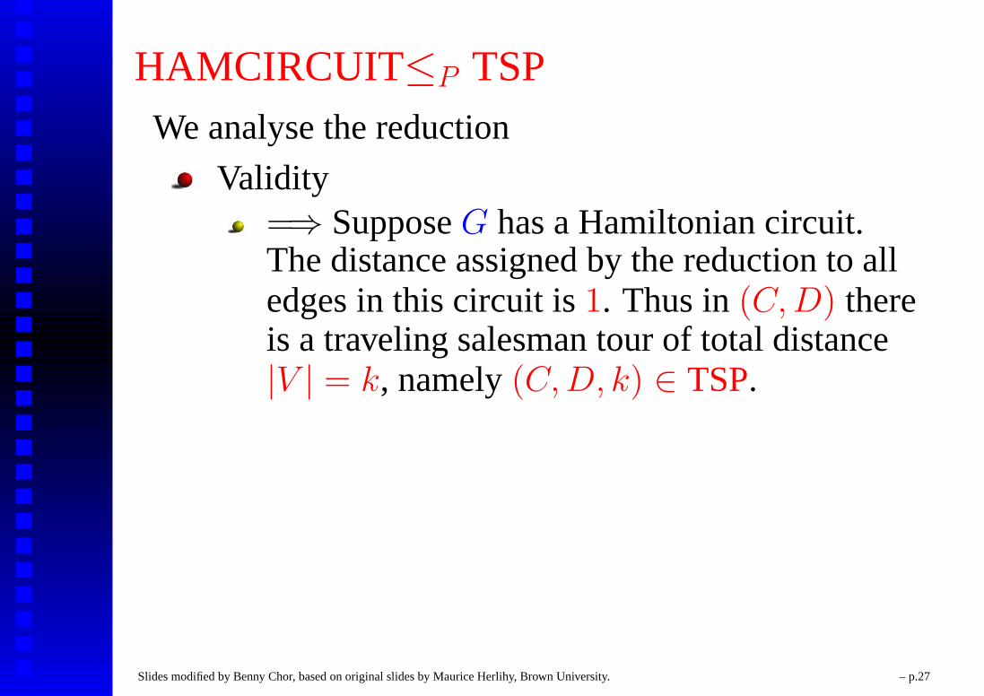
HAMCIRCUIT≤P TSPWe analyse the reduction
Validity
=⇒ Suppose G has a Hamiltonian circuit.The distance assigned by the reduction to alledges in this circuit is 1. Thus in (C,D) thereis a traveling salesman tour of total distance|V | = k, namely (C,D, k) ∈ TSP.⇐= Suppose (C,D) has a traveling salesmantour of total distance |V | = k. Tour cannotcontain any edge of distance 2. Therefore itgives a Hamiltonian circuit in G.
Efficiency: Reduction in quadratic time (filling updistances for all edges of the complete graph). ♣
Slides modified by Benny Chor, based on original slides by Maurice Herlihy, Brown University. – p.27
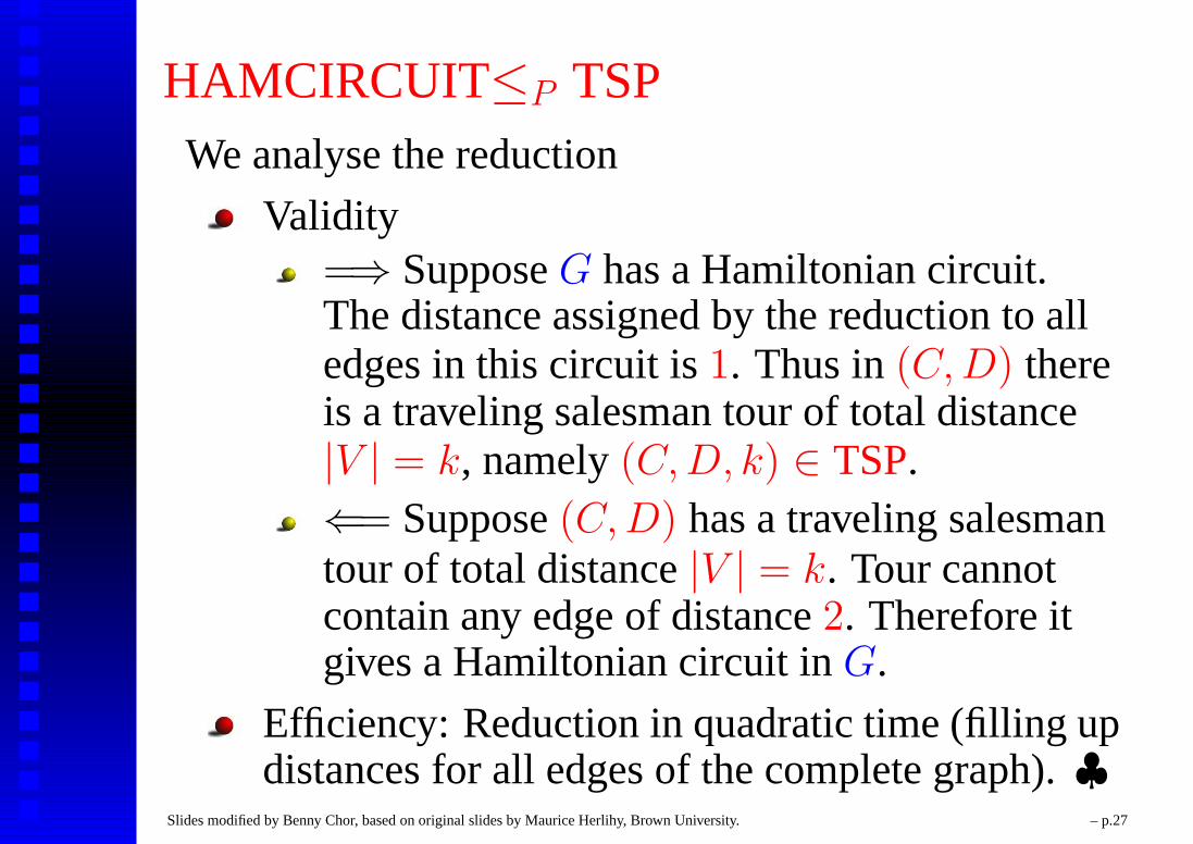
HAMCIRCUIT≤P TSPWe analyse the reduction
Validity=⇒ Suppose G has a Hamiltonian circuit.The distance assigned by the reduction to alledges in this circuit is 1. Thus in (C,D) thereis a traveling salesman tour of total distance|V | = k, namely (C,D, k) ∈ TSP.
⇐= Suppose (C,D) has a traveling salesmantour of total distance |V | = k. Tour cannotcontain any edge of distance 2. Therefore itgives a Hamiltonian circuit in G.
Efficiency: Reduction in quadratic time (filling updistances for all edges of the complete graph). ♣
Slides modified by Benny Chor, based on original slides by Maurice Herlihy, Brown University. – p.27

HAMCIRCUIT≤P TSPWe analyse the reduction
Validity=⇒ Suppose G has a Hamiltonian circuit.The distance assigned by the reduction to alledges in this circuit is 1. Thus in (C,D) thereis a traveling salesman tour of total distance|V | = k, namely (C,D, k) ∈ TSP.⇐= Suppose (C,D) has a traveling salesmantour of total distance |V | = k. Tour cannotcontain any edge of distance 2. Therefore itgives a Hamiltonian circuit in G.
Efficiency: Reduction in quadratic time (filling updistances for all edges of the complete graph). ♣
Slides modified by Benny Chor, based on original slides by Maurice Herlihy, Brown University. – p.27
Hamiltonian PathTheorem: HAMPATH is NP-complete.
Must demonstrate
HAMPATH ∈ NP
every A ∈ NP poly-time reducible toHAMPATH.
Note thatwe have already seen the firstwill now show that 3SAT ≤P HAMPATH
Slides modified by Benny Chor, based on original slides by Maurice Herlihy, Brown University. – p.28
Hamiltonian PathTheorem: HAMPATH is NP-complete.
Must demonstrate
HAMPATH ∈ NP
every A ∈ NP poly-time reducible toHAMPATH.
Note thatwe have already seen the firstwill now show that 3SAT ≤P HAMPATH
Slides modified by Benny Chor, based on original slides by Maurice Herlihy, Brown University. – p.28

Hamiltonian PathTheorem: HAMPATH is NP-complete.
Must demonstrate
HAMPATH ∈ NP
every A ∈ NP poly-time reducible toHAMPATH.
Note that
we have already seen the firstwill now show that 3SAT ≤P HAMPATH
Slides modified by Benny Chor, based on original slides by Maurice Herlihy, Brown University. – p.28

Hamiltonian PathTheorem: HAMPATH is NP-complete.
Must demonstrate
HAMPATH ∈ NP
every A ∈ NP poly-time reducible toHAMPATH.
Note thatwe have already seen the first
will now show that 3SAT ≤P HAMPATH
Slides modified by Benny Chor, based on original slides by Maurice Herlihy, Brown University. – p.28

Hamiltonian PathTheorem: HAMPATH is NP-complete.
Must demonstrate
HAMPATH ∈ NP
every A ∈ NP poly-time reducible toHAMPATH.
Note thatwe have already seen the firstwill now show that 3SAT ≤P HAMPATH
Slides modified by Benny Chor, based on original slides by Maurice Herlihy, Brown University. – p.28

Hamiltonian PathFor any 3CNF formula φ,
we construct a graph G
with vertices s and t
such that φ is satisfiable iff there is a Hamiltonianpath from s to t.
Slides modified by Benny Chor, based on original slides by Maurice Herlihy, Brown University. – p.29

Hamiltonian PathFor any 3CNF formula φ,
we construct a graph G
with vertices s and t
such that φ is satisfiable iff there is a Hamiltonianpath from s to t.
Slides modified by Benny Chor, based on original slides by Maurice Herlihy, Brown University. – p.29

Hamiltonian PathFor any 3CNF formula φ,
we construct a graph G
with vertices s and t
such that φ is satisfiable iff there is a Hamiltonianpath from s to t.
Slides modified by Benny Chor, based on original slides by Maurice Herlihy, Brown University. – p.29

Hamiltonian PathHere is a 3CNF formula φ:
(a1 ∨ b1 ∨ c1) ∧ (a2 ∨ b2 ∨ c2) ∧ · · · (ak ∨ bk ∨ ck)∧
where
each ai, bi, ci is xi or xi
the ` clauses are C1, . . . , C`,
the k variables are x1, . . . , xk.
Slides modified by Benny Chor, based on original slides by Maurice Herlihy, Brown University. – p.30

Chains of Reductions: NPC Problems
SAT
IntegerProg 3SAT
Clique
IndepSet
VertexCover
SetCover
3ExactCover
Knapsack
Scheduling
3Color HamPath
HamCircuit
TSP
Slides modified by Benny Chor, based on original slides by Maurice Herlihy, Brown University. – p.31

On Search, Decision, and Optimization
Let R(·, ·) be a poly time computable predicate.
Decision Problem: Given input x, decide if thereis some y satisfying R(x, y)?
Using the “certificate” characterization oflanguages in NP, the decision problem is the sameas deciding membership x ∈ L for L ∈ NP .
Search Problem: Given input x, find some ysatisfying R(x, y), or declare that none exist.
The search problem seems harder to solve thanthe decision problem.
Slides modified by Benny Chor, based on original slides by Maurice Herlihy, Brown University. – p.32
On Search, Decision, and Optimization
Search Problem: Given input x, find some ysatisfying R(x, y), or declare that none exist.
The search problem seems harder to solve thanthe decision problem.
Turns out that for NP complete languages, searchand decision have the same difficulty.
Specifically, given access to an oracle for L (thedecision problem), we can solve the searchproblem in poly time.
Examples: SAT and Clique (on board).
Slides modified by Benny Chor, based on original slides by Maurice Herlihy, Brown University. – p.33
![Modern SAT Solvingsat.inesc-id.pt/~ines/cp07.pdf · 2010. 3. 4. · SAT is an NP-complete decision problem [Cook’71] { SAT was the rst problem to be shown NP-complete { There are](https://img.dokumen.tips/doc/110x75/60fe5bc839d3824bba4d66d1/modern-sat-inescp07pdf-2010-3-4-sat-is-an-np-complete-decision-problem.jpg)