The Labor Market Effects of Reducing

Undocumented Immigrants

Andri Chassamboulli (University of Cyprus)

Giovanni Peri (University of California, Davis)∗

February, 14th, 2014

Abstract

A key controversy in US immigration reforms is how to deal with undocumented

workers. Some policies aimed at reducing them, such as increased border security

or deportation will reduce illegal immigrants as well as total immigrants. Other

policies, such as legalization would decrease the illegal population but increase the

legal one. These policies have different effects on job creation as they affect the

firm profits from creating a new job. Economists have never analyzed this issue.

We set up and simulate a novel and general model of labor markets, with search

and legal/illegal migration between two countries. We then calibrate it to the US

and Mexico labor markets and migration. We find that policies increasing deporta-

tion rates have the largest negative effect on employment opportunities of natives.

Legalization, instead has a positive employment effect for natives. This is because

repatriations are disruptive of job matches and they reduce job-creation by US firms.

Legalization instead stimulates firms’ job creation by increasing the total number

of immigrants and stimulating firms to post more vacancies some of which are filled

by natives.

JEL code: F22, J61, J64.

KeyWords: job creation, bargaining power, undocumented immigrants, border

controls, deportations, legalization, unemployment, wages.

∗Andri Chassamboulli, Departement of Economics, University of Cyprus, CY-1678 Nicosia; an-dricha@ucy.ac.cy. Giovanni Peri, Department of Economics, UC Davis. One Shields Avenue, Davis

Ca 95616 USA; gperi@ucdavis.edu.

1

1 Introduction

The current theoretical and empirical literature on the labor market effects of immigra-

tion considers the number of immigrants as an exogenous variable. Most studies, then

analyze the consequences of increasing the number and/or changing the skill distribution

of immigrants on native labor market outcomes. The number and type of immigrants

entering a country, however, is not a “policy variable”. It is the outcome of economic and

social pull forces and policy barriers and controls. Nevertheless, in the economic literature

on the effect of immigration, very little attention is paid to the specific policies used to

influence immigration and their potentially different effects on labor markets. Moreover,

those analysis rarely differentiate between legal and illegal immigrants and their effects

on natives.

If one moves outside of academia, however, the perception of legal and illegal immi-

gration is sharply differentiated, with most people and politicians approving of (and often

praising) legal immigrants but many of them strongly criticizing (and often vilifying) il-

legal ones. Moreover a large part of the very vigorous policy debate, in the US, is around

what policies should be used to reduce the number of (or ideally eliminate) undocumented

immigrants in the United States. Everybody agrees that the presence of undocumented

is an anomaly to be solved but there is harsh disagreement on how to solve it. Is border

enforcement the only policy needed? What would be the solution for those already in

the US? Will we need massive deportation? or "self deportation"? or is legalization the

most reasonable and practical option and what are its long-run consequences? These are

the main issues that (as we write) generate disagreement and bog down any possibility of

immigration reform.

There is also a very clear perception that the US government should consider these

policies not only based on the effectiveness in reducing the number of undocumented

immigrants but also with an eye to the other consequences that policies would have. First,

the effects on undocumented immigrants (their rights and safety) should be considered.

Equally important, however, are their effects on labor markets opportunities of US workers

and on the economic success of US firms: will fewer illegal immigrants free jobs for

Americans or cause firms to close? Moreover, the incentive that these policies can produce

on perspective immigrants should be considered: will legalization cause a wave of new

immigrants? Economists, so far, have not produce a framework to analyze quantitatively

these effects in a coherent structure and hence they have been marginal to this debate.

1

This paper begins to fill this gap.

We propose a novel model representing two connected labor markets (parameterized,

in the quantitative analysis, to be those in US and Mexico), in which workers search

for employment. Firms create jobs and search frictions in the market exist. Legal and

Illegal migration opportunities arises from the poor to the rich country because of working

incentives. This model, that incorporates several crucial realistic aspects of labor markets

and migration, which would not be captured by a classical demand-supply framework, is

used to analyze different policies aimed at reducing illegal immigration. The quantitative

predictions of the model are used to evaluate the labor market implications on natives

and immigrants, of different policies to reduce undocumented Mexican immigrants in the

US.

The model builds on the search and job-posting model of Chassamboulli and Palivos

(forthcoming) and extends it to two countries. We also include the migration decision and

we endogenize it as function of several policy parameters and of labor market conditions.

The possibility of migration creates economic opportunities to the potential migrants of

the poorer country as they can increase their salary and the value of search. It also creates

opportunities to the firms of the richer country who could hire immigrants at lower salary

cost, increasing their profits and the value of job posting. While firms in the rich country

and workers in the poor country are helped by migration, the group of workers in the rich

country can be hurt by immigration, as competition on the labor market may become

steeper. However, the model shows that a larger share of immigrants and the option of

hiring them drives the rich country firms to create more job-openings. This is because la-

bor market frictions generate match-specific surplus and, as immigrants are paid less than

natives (because of their a worse outside option), a larger share of immigrants increases

the expected profit from creating a job. This drives firm to create more jobs. Some native

workers are employed (ex-post) in some of those job-openings. Hence, in equilibrium,

more immigrants produce (for reasonable parameter values) lower unemployment rates

and higher wages for natives because they stimulate higher job creation per unemployed.

In this framework, undocumented immigration that allows access to the labor market

of the rich country, albeit at worse conditions and with the risk of deportation, can be

attractive for poor country’s workers and for rich country’s firms. Cheaper workers are

available, firms increase their profit and more jobs are created. These features seem to

capture exactly the economic incentives that have lead to undocumented immigration in

2

the US. The paper asks: how can we reduce undocumented immigration in the least costly

way for US firms and workers?

The four policies that we analyze are the following: (i) Reducing the opportunities

of illegal immigration (more border enforcement), (ii) increasing the costs that undocu-

mented face in looking for a job (hostile environment, no access to any social benefits),

(iii) increasing the frequency of deportations and, finally, (iv) increasing legalization rates

sometimes called "amnesty". In looking at the labor market effects of these policies, legal

immigrant, illegal immigrant and native workers are considered to be equally productive

and perfect substitutes in production, so that we can focus on their differences in terms

of outside options and bargaining positions as driver of the outcomes. Immigrants, in

fact have different outside options and hence different wages from natives in equilibrium,

even for identical productivity. We assume that job posting by a firm cannot target a

specific type of worker in terms of nativity and immigration status. However different

workers can be paid different salaries once the match is realized, because of their different

bargaining position. We endogenize migration incentives by considering that workers in

the poor country search for migration opportunities (as well as for local jobs). They take

them if the expected benefit from those, net of migration costs, is larger than the expected

value of continuing to search for a domestic job. Heterogeneity across individuals in their

emigration costs implies that only a fraction of poor-country workers will migrate.

While we show and discuss some analytical results, our key results are obtained from

simulations. We use a set of parameters from the literature and we calibrate the remaining

to match the average moments of the US and Mexico labor market and migration vari-

ables (wages, employment rates, migration and return rates for legal and illegal migrants,

unemployment benefits) for the 2000-2010 period. Then we simulate changes in each

policy to achieve a certain percentage reduction of undocumented and we calculate the

corresponding effects on labor market outcomes. The first important implication of our

model is that, as legal immigrants and (even more) illegal immigrants have worse outside

options than natives, a larger share of either group in the labor force of the richer country

increases the profits of firms, and hence job creation. Market tightness is higher with a

larger share of immigrants, which implies lower unemployment rates and higher wages

for natives workers too. These two results (first shown in Chassamboulli and Palivos,

forthcoming) stem from the job-creation side of the economy. They are present as long as

immigrants receive lower wage per unit of productivity, because of their worse outside op-

3

tion/lower bargaining power. This is a very reasonable assumption, supported by a large

body of empirical work that shows immigrants earning lower wages than natives, even

when controlling for all observables.1 Interestingly, this implies that immigration policies

reducing overall immigration have a negative effect on employment and wages of natives.

Moreover policies have a particularly bad effect on job creation if they also reduce the

surplus that firms obtain from hiring illegal immigrants. For these reasons, deportation

has the most disruptive and negative effect on the labor market. Increasing the deporta-

tion rate, in fact, reduces the number of illegal and overall immigrants; it also reduces the

value of hiring an undocumented to a firm (as it increases the probability of breaking the

match due to deportation). As such, for a given reduction of undocumented immigrants,

increased deportation usually generates a strong negative job-creation effect on US firms

and hence the largest negative impact on the wage and employment of natives. To the

other end of the spectrum, legalization, by decreasing undocumented but not decreas-

ing the total number of immigrants and not altering significantly the surplus for a firm

from hiring an undocumented, has the smallest negative effect on job creation. In fact,

under reasonable parameter values, legalization produces an increase in total immigrants

and it provides a job-creating stimulus by increasing the expected profit of job creation.

Legalization increases the number of legal immigrants because some illegal are legalized

and also because the value of migrating increases and more migrants are attracted to the

richer country. Hence legalization produces a reduction in undocumented with actually

positive labor market effects for natives (higher wages and lower unemployment rate).

Reducing illegal immigration opportunities (border enforcement) and increasing the cost

of job search for undocumented (hostile environment) have also negative effect on wages

and employment of natives. Their magnitude is similar to, albeit smaller than, the effects

of deportation.

The main quantitative implications of our simulations are that by increasing the de-

portation rate of immigrants to achieve a 50% reduction in their number would produce an

increase in the native unemployment rate by about 1.6% of its initial value. The wage of

natives would be reduced by 0.08% of their value. However, the same reduction achieved

with a legalization program would produce a decrease in the native unemployment rate

by about 4% of its initial value and it would increase native wages by 0.19% of their initial

value. Several robustness checks and extensions are provided and they do not change the

1See for a survey Kerr and Kerr (2011).

4

main results.

The rest of the paper is organized as follows. Section 2 reviews the existing literature

on undocumented immigration and labor market outcomes especially within the frame of

search and matching models. Section 3 presents the model and provides intuition for its

main results and the working of different mechanisms. We then describe in Section 4 the

policy experiments that we will be considering. Section 5 describes the parameterization

of the model calibrated to match the main labor market statistics of the US and Mexico for

the period between 2000 and 2010. Section 6 shows the main effects obtained by simulating

four different policies that would achieve a reduction of the number of undocumented

immigrants in the rich country. In Section 7 we present some checks that the results

are robust to reasonable variations of the parameter values and we show an extension to

the model to the case in which illegal immigrants have no bargaining power. Section 8

concludes the paper.

2 Literature Review

There is a vast empirical literature on the effect of immigration on US labor market

outcomes (see the Meta-Analysis by Longhi, Nyikamp and Poot (2005), (2008) for a

review of several important recent findings). Most of it uses a simple neoclassical labor

demand-supply approach to derive a reduced form equation (e.g. Borjas 2003) or a slightly

more structural approach to estimate elasticity of relative demand (Ottaviano and Peri

2012, Manacorda et al 2012). Very few studies analyze immigration within the context of

search-matching models of the labor market. Even fewer explicitly differentiate between

legal and illegal immigration when looking at labor market implications.

The paper most closely related to ours is Chassamboulli and Palivos (forthcoming).

In that paper immigration is exogenous, only the receiving country is analyzed and only

legal immigrants exists. The labor market consequences on native workers are analyzed

using a search and matching model, which provides the basis for the model in this pa-

per. Chassamboulli and Palivos (forthcoming) simulate the effects of different inflows of

immigrants and identify the important job-creation effect of immigrants stemming from

the fact that the surplus generated by immigrants for the firm is larger than the surplus

generated by natives because their wages are lower. The novelties of this paper, relative

to that contribution is that we explicitly model the migration decision from Mexico, that

we allow for undocumented immigrants characterized by higher labor search costs and

5

risk of deportation and that we analyze the effect of specific policies.

Palivos (2009) is one of the very few papers analyzing the welfare effects of undoc-

umented immigrants on natives. Liu (2010) is the only other model, to the best of

our knowledge, that analyzes the effects of undocumented immigration on the receiving

country using a search and matching model. In his model, Liu (2010), only includes un-

documented immigrants and assumes that they are identical to natives in their search and

labor supply behavior, but may be complementary to native workers in production. We

consider, instead that immigrants, and particularly undocumented, are disadvantaged rel-

ative to natives in terms of job search conditions and unemployment benefits (they receive

lower or no benefits) and we include also the possibility that undocumented are subject

to the risk of deportation. In our model what is commonly refereed to as “exploitation”

of undocumented, namely them being paid lower salaries, is due to their worse bargaining

position vis-a-vis their employer relative to natives.

Also somewhat related to this paper, although mainly empirical, is the literature on

immigration and labor market institutions. It has been recognized for some time that

the specific labor market institutions (level of unemployment benefits, costs of hiring,

centralization of wage bargaining) can affect significantly the impact of immigration on

employment and wages of natives. E.g. Angrist and Kugler (2003) show that more pro-

tective labor markets result in larger impact of immigration on unemployment. D’Amuri

and Peri (2013) also show that labor reallocation and wage effects can be larger in markets

with lower rigidities.

3 The Model

We describe here the main features of the model. The details and the derivation of the

specific equations are described in the Appendix (A). We consider two countries indexed

using the subscript = [1 2] Each country is endowed with a continuum of workers. All

agents are risk neutral and discount the future at a common rate 0 equal to the

interest rate. Time is continuous. In absence of migration, country 1 has higher wages

and more employment opportunities than country 2. Hence, when migration is allowed,

some workers have incentives to migrate from country 2 to country 1 to maximize their

income. No worker has incentives to migrate from country 1 to country 2. Migration

can be legal (authorized) or illegal (unauthorized). We denote with and respectively,

the number of illegal and legal migrant workers in country 1. The labor force born in

6

country 1, natives (), is normalized to 1 while individuals born in country 2 are of

measure (foreign). The total labor force of country 1 consists of natives, legal and

illegal immigrants and is given by 1 + +. The measure of total labor force in country

2 is − − . As they turn out to be crucial variables we also define to be the share

of native workers in the unemployment pool of country 1 and to be the share of legal

among unemployed immigrants of country 1.

In each period, opportunities to migrate are “random draws” occurring at rate ,

if the worker is employed in country 2, and at rate , if the worker is unemployed.

The subscript = [ ] indicates the type of the immigration opportunity. Specifically,

the worker may find an opportunity to immigrate to country 1 legally () or illegally

(). Once in country 1, illegal immigrants face the risk of deportation. They may also

obtain legal status with probability , reflecting the possibility that, even in absence of

amnesty, marriage or other special circumstances would allow them the opportunity to

naturalize. We assume that and we standardize = 0, = [ ] Migration

opportunities arise only for the unemployed, who are actively looking for them. This

captures the idea that, in order to migrate, workers often need to move closer to the

border and actively look through their networks for migration opportunities. A worker

will take up an opportunity to migrate to country 1 only if the benefit exceeds the cost.

The migration cost is heterogeneous across individuals and it is distributed according to

the CDF Φ(·) with support [ ]. Only the fraction of workers with costs lower thanexpected benefits is willing to migrate. Migration opportunities are not the same as job

opportunities in the rich country. Immigrants still need to search for a job, even if for

a short time, once in country 1. Hence, the benefit from immigrating to country 1 is

the difference between the value of being unemployed (i.e. searching for a job) as an

immigrant in country 1 and the value of being unemployed as a native in country 2.2

3.1 Search and Matching

Each of the two countries represents a labor market. In each labor market unemployed

workers and unfilled vacancies are brought together via a stochastic matching technology

( ) where and denote, respectively, the number of unemployed workers and

vacancies in country = [1 2]. We assume that the function (·) exhibits properties2One could think of a model in which firms in country 1 can directly hire workers in country 2 and

hence these persons emigrate already with a job. This, however, would imply a really global labor market

in which firms posts vacancies accessible to all workers in any country and this seems hardly realistic.

7

standard in the labor search literature: it is at least twice continuously differentiable,

increasing in its arguments, it exhibits constant returns to scale and it satisfies the Inada

conditions. Using the property of constant returns to scale, we can write the flow rate of

a match for an unemployed worker as( ) = (). The flow rate of a match for

a vacancy is( ) = (), where = = ()() represents the measure

of market tightness.

Each firm posts at most one vacancy. The number of vacancies in each market is

determined endogenously by free entry. Firms’ vacancies cannot be specifically “labelled”

for natives or for immigrants only. They are open to all workers. A vacant firm bears

a recruitment cost specific to the country, related to expenses of keeping a vacancy

and looking for a worker. An unemployed worker in country receives a flow of income

, which can be considered as the opportunity cost of employment, and in addition,

pays a per unit of time search cost , where the subscript = [ ] denotes the

worker’s origin and status: native (), illegal immigrant () and legal immigrant ().

This status-specific cost allows us to account for the fact that an immigrant worker may

face a higher search cost compared to a native worker because he/she is eligible for fewer

benefits when unemployed (unemployment insurance, health care, welfare) especially if

undocumented. We standardize the search cost of a native worker to 0 and we assume

that legal immigrants face lower search cost than illegal immigrants. Specifically, we set

1 = 2 = 0, 1 = , 1 = and 0.

As already mentioned, legal immigrants face zero deportation risk. They have a posi-

tive probability of returning home reflecting the possibility of return for personal, family-

related or other reasons. Illegal immigrant face the additional risk of being repatriated by

deportation. Hence the return probability of illegal immigrants is higher than that of legal

immigrants. Let and denote the instant return rate of legal and illegal immigrants,

respectively. We set ≥ 0 where their difference is the deportation rate. Following

return the worker joins the pool of unemployed (in country 2) and starts searching for a

job.

When a vacancy and a worker are matched, they bargain over the division of the

produced surplus. The status of the worker as well as the output that results from a match

are known to both parties. In country matches produce output , irrespective of the

worker’s origin and legal status. Hence we are considering workers of similar productivity

differing only in their immigration status. Wages, on the other hand, denoted as differ

8

by country ()and migration status () and are determined by Nash bargaining, where

the worker has bargaining power After an agreement has been reached, production

commences immediately. Moreover, we assume that matches dissolve at the rate

specific to country . Following a job destruction, the worker and the vacancy enter the

corresponding market and search for new trading partners.

3.2 Bellman Equations and Free Entry

At each point in time a worker is either employed () or unemployed (), while a vacancy

may be either filled ( ) and producing or empty and searching for a worker ( ). We use

the common notation to denote the present discounted value associated with each

state = [ ], where = [1 2] denotes the country and = [ ] the worker’s

immigration status. Hence in steady state we have fourteen Bellman equations. Four of

them describe the value of Employment and four of them the value of Unemployment

for workers of each type in each country (eight conditions in total). As for firms, there

are four conditions for the value of a filled vacancy (depending on country and type of

worker) but only two conditions for the value of unfilled vacancies (one in each country)

because unfilled vacancies are open to any worker and not specific to a type. The full set

of Bellman equations is in the Appendix A.

While the interested reader could inspect the equations in the Appendix for details let

us provide here some intuition of how this model differs from a standard one-country model

of search and matching. First, the possibility of finding an opportunity for entry into

country 1 (either legal or illegal) increases the value of being unemployed for a country-

2 worker relative to the case of closed borders. The net benefit of migrating legally is

represented by the difference between the values of being an unemployed legal migrant

in country 1 and being unemployed in country 2 net of migration costs: 1 −

2 −

where is the individual-specific migration cost. Migrating illegally yields 1 −

2 − .

If the net benefit of migrating is smaller than 0 the worker will continue his search in

country 2.3 Second, the exogenous probability of return (because of unforeseen events or

due to deportation) affects negatively the value of being an immigrant to country 1. In

the event of a return, in fact, the immigrant will either have to quit his job (if currently

employed) or give up searching for a job in country 1 (if currently unemployed) and join

3The assumption that only unemployed workers can draw migration opportunities to country 1 is not

restrictive. Allowing also employed workers to migrate, however, will produce a different migration cost

threshold for employed and unemployed, making the problem notationally cumbersome.

9

the pool of unemployed workers in country 2. We know, from the migration condition,

that this passage implies a loss in value. Specifically, the cost of return for an unemployed

(employed) immigrant is given by 2 −

1 (2 −

1), if legal, and 2 −

1 (2 −

1), if

illegal.4 The presence of this exogenous return probability, due to shocks (or deportation

for illegal aliens) allows us to incorporate return migration in the model, even if it is

economically advantageous for migrants to stay in country 1.

A third important feature of this model is that the value of being unemployed in

country 1 is higher for native than for immigrants in spite of identical productivity for

two reasons. First, immigrants face the “risk” of return which would force a separation

from their job. Second, we assume that immigrants pay a positive search cost denoted

as with = [ ] representing their worse conditions when unemployed. Hence their

flow-unemployment value (1−) is smaller than that of natives (1). The same reasoningalso explains why the value of unemployment to an immigrant worker is lower when that

immigrant is illegal (1) than when legal (

1): an illegal immigrant faces a higher search

cost ( ) and a higher risk of return due to deportation ( ).

Exogenous return-events are costly not only to the immigrant workers but also to the

firm that employs them. Following return, the job becomes vacant and the firm has to

undertake costly search. Hence, a firm employing an illegal (or a legal) immigrant will

incur a net cost 1 −

1 (1 −

1), when the workers returns to the home country. Jobs

filled by immigrants face a higher separation probability than jobs filled by natives and

this feature makes them less valuable to the firm. However, their worse outside option

implies that they are paid lower wage and this features makes them more valuable to the

firm.

Finally we allow for the possibility that an illegal immigrant is legalized (with prob-

ability ). In this case the immigrant receives a surplus 1 −

1 , if unemployed and

1 −

1 , if employed. Obtaining the legal status always yields a positive surplus to the

immigrant worker, because as mentioned above, legal immigrants do not face deportation

risk and have lower search costs. For the firm, on the other hand, legalization of an

employee has two opposite effects. On the one hand firms have to pay higher salary to

legalized workers, as their outside options have improved. On the other hand they are

less likely to be separated from the jobs which makes the match more valuable. The net

effect will depend on the relative size of those effects.

4Since 1 2 , it must be the case that 1 2 , because

1 1.

10

We assume free-entry on the firm side in each of the two labor markets (country 1 and

2). Hence firms continue to open vacancies up to the point that an additional vacancy

makes zero expected profit. In equilibrium this free-entry condition implies:

= 0 = [1 2] (1)

3.3 Nash Bargaining

Wages are determined by a Nash bargain between the matched firm and worker. The

threat points of the firm and the worker are simply the value of a vacancy and the value

of being unemployed, respectively. Let ≡ +

− ( +

) denote the surplus

of a match between a vacancy and a worker of immigration status in country . With

Nash-bargaining the wage is set to a level such that the worker gets a share of the

surplus, where represent the relative bargaining power of workers, and the remaining

goes to the firm.5 That is:

= −

(1− ) = −

(2)

3.4 The Immigration Decision

An (unemployed) worker located in country 2 will choose to immigrate to country 1,

when an immigration opportunity arises, if its benefit exceeds its cost. The benefit from

migration, as described above, is the difference between the value of searching (being

unemployed) in country 1 and the value of searching in country 2. Workers are hetero-

geneous in their migration costs. A worker whose migration cost is , will chose to take

advantage of an opportunity to enter legally in country 1 only if 1−

2 ≥ while he/she

will enter illegally if 1 −

2 ≥ . The highest immigration costs that a worker (located

in country 2) is willing to pay in order to obtain illegal or legal entry into country 1, are

denoted by ∗ and ∗, respectively, and they are:

∗ = 1 −

2 (3)

∗ = 1 −

2 (4)

5Notice that in this baseline specification we assume that native, legal and illegal immigrants have

the same relative power in the Nash-bargaining. Still the wage of legal and illegal immigrants are lower

than those of natives because of their worse outside options. In Section 7 we explore the case that illegal

immigrants have no bargaining power and receive a take-it-or leave it offer.

11

Notice that ∗ ∗ , because, as mentioned above, the value of searching for a job in

country 1 is higher when the immigrant is legal than when he/she is illegal (i.e. 1

1).

Intuitively, the benefit from legal entry is higher than that of illegal entry, thus a worker

is willing to incur a higher cost in order to obtain the right for legal entry. This also

implies that for a given distribution of the migration cost , in the population, there will

always be a larger share of the country 2 population willing to take a legal immigration

opportunity than an illegal one.

3.5 The Steady-state Unemployment and Migration Rates

The steady-state conditions determine the stationary number of unemployed (native)

workers in country 2, 2, the number of unemployed natives in country 1, 1 , and the

number of unemployed legal and illegal immigrants in country 1, 1 and 1 . The formal

conditions are given by (41-44) in the Appendix A.2 and they state that flows into and

out of unemployment status for each type of worker in country 1 and in country 2 should

be equal.

Two more conditions guarantee the stationarity of the number of legal and illegal

immigrants, and and hence of their share in unemployment, and . By equating

the inflow of new legal immigrants, which includes the inflow of new immigrants and

the legalization of incumbents, to the outflow of legal immigrants returning to the home

country, we obtain the steady-state condition for :

= + 2Φ(∗) (5)

Likewise, the steady state condition for the number of illegal immigrants, , implies that

the inflow of new illegal immigrants equals the flow of illegal immigrants that either return

home or obtain the legal status:

( + ) = 2Φ(∗ ) (6)

The conditions (5), (6) above and those expressing stationarity of unemployment rates

(45-48 in the Appendix) can be combined to write the steady-state numbers of illegal and

legal immigrants as:

=Φ(

∗ )2( − )

+ + Φ(∗ )2

(7)

=Φ(

∗)2( − ) +

+ Φ(∗)2

(8)

12

As expected, the equilibrium number of legal (illegal) immigrants increases (decreases)

with the legalization rate The number of immigrants of each type (legal or illegal)

decreases with the respective return rate and increases with the respective entry rate.

Moreover, a change in parameters leading to an increase (decrease) in , namely an

increase (decrease) in Φ(∗) or a decrease (increase) in , have a negative (positive)

impact on , because a larger (smaller) number of legal immigrants means a smaller

(larger) pool of workers located in country 2 available to enter illegally into country 1.

However, the converse is not always true. The impact of an increase in Φ(∗ ) or a

decrease in , both of which increase is not always negative on . While the change in

those two parameters implies a smaller pool of workers in country 2, available to migrate

legally, they also increase the pool of , some of whom become legal immigrants themselves

through legalization (). If the rate at which existing illegal immigrants become legal is

larger than the rate at which the natives of country 2 enter legally into country 1, i.e.

if Φ(∗)2, then an increase in will have a positive impact on . Hence, an

increase in the entry rate of illegal immigrants (Φ(∗ )2), or an decrease in their return

rate () will have an unambiguously positive impact on and a negative impact on

only if Φ(∗)2.

6

Notice, very importantly, that the economic and policy conditions in country 1, rel-

ative to country 2, affect the incentives to migrate legally and illegally (and hence the

equilibrium stock of migrants and ) via their effect on the threshold migration costs

∗ and ∗. In particular, as expressed very clearly by conditions (3) and (4), any eco-

nomic and policy factor that increases the value of being unemployed (through the value

of being employed) in country 1 relative to country 2, will encourage immigration. This,

in equilibrium, translates in larger stocks of legal and illegal immigrants in country

1. Hence this model allows us to evaluate immigration policies accounting for the direct

effect on immigrants (through altering the flows into each state) as well as for their indi-

rect “incentive” effects on potential documented and undocumented immigrants, via the

impact on return to migration. This is a novel and important feature of this model.

6The results derived here assume that both legal and illegal migrants loose their status in country 1

once they return to country 2 and they have to look for a new opportunity (legal or illegal) to go back

to country 1 in a new status.

13

3.6 Equilibrium

3.6.1 Wages

Using the Bellman equations (27) to (40), the zero-expected-profit (free entry) conditions

(1) the Nash bargaining conditions (2) and the immigration conditions in (3) and (4),

we can solve for the equilibrium wage rates. Those are specific to each type of worker

in country 1 (native, legal and illegal immigrants) and to workers of country 2. Their

expressions are as follows7:

1 = 11 + (1−1)1 (9)

1 = 11 + (1−1) (1 − ) (10)

1 = 11 + (1−1) (1 − ) + Γ1 (11)

2 = 22 + (1−2)

µ2 +

Z ∗

(∗ − )Φ() +

Z ∗

(∗ − )Φ()

¶(12)

where 1 ≡ (+1+(1))+1+(1)

, 1 ≡ (+1++(1))+1++(1)

, 1 ≡ (+1+++(1))+1+++(1)

, 2 ≡(+2+(2))+2+(2)

and Γ ≡ (1)+1+++(1)

.

One can verify by inspecting equations (9) to (12) that an increase in the separation

rate of a match, either due to an increase in the exogenous return probability of immigrants

( or ) or due to an increase in the probability of separation (), has a negative impact

on the worker’s wage. This is because an increase in the separation probability lowers

the expected duration of a match and therefore the surplus received from the job ().

Since wages are such that the firm and the worker split the expected surplus in fixed

proportions, a decrease in the job surplus implies also a decrease in the worker’s share of

surplus (recall that −

= ) and thus a decrease in the worker’s wage.

Inspection of (9) and (10) also shows that the equilibrium wage of a native worker

is higher than that of a legal immigrant worker i.e. 1 1 despite the fact that

they are all equally productive. This happens for two reasons. The first reason stems

from the different outside option: immigrants face a higher search cost (i.e. 0),

which forces them to accept lower wages. This effect is captured by the second term in

the wage expression. The second reason relates to the disruptive effects that exogenous

return shocks have on the values of jobs. Because working immigrants have a positive

probability of exogenous return 0, jobs filled by immigrants have shorter expected

7A more intuitive expression of wages that helps to understand their dependence on productivity and

outside options is presented in Appendix A.3.

14

duration than jobs filled by natives. Hence, they generate a smaller surplus and thus

earn lower wages. This effect can be seen by noticing that 1 1 and hence the

native wage puts more weight on the (larger) term 1 The same two reasons contribute

to making the wage of illegal lower than the wage of legal immigrants. Their search cost

is even higher than of legal immigrants (i.e. ), and because they can be deported

their probability of return is higher than for legal immigrants (i.e. ).

3.6.2 The immigration costs threshold

Using equations (34), (35), (36), the zero-expected-profit conditions (1) and the Nash bar-

gaining conditions (2) we can write the equilibrium conditions for ∗ and ∗ in equations

(4) and (3) as follows:

( + )∗ + (∗ − ∗) + = 1 − 2 − + Γ [(1 − 1)(1 + Γ) + + Γ]

− 22(1− )

(13)

( + )∗ + = 1 − 2 − + Γ(1 − 1 + )− 22

(1− )(14)

where Γ is defined above while ≡ R ∗(∗ − )Φ() +

R ∗(∗ − )Φ() and

Γ =(1)

+1++(1). These two equations can be used to solve for ∗ and ∗ in terms of

1, 2 and model parameters. The cost thresholds ∗ and ∗ determine the rate at which

natives of country 2 migrate into country 1. In equilibrium they are equal to the (illegal

and legal) immigration surplus, namely the difference between the value of searching for

a job in country 1 and the value of searching for a job in country 2. When the benefit

from illegal (legal) entry into country 1 increases, then ∗ (∗) also increases and a larger

share of country-2 workers accept opportunities for illegal (legal) entry. Hence their inflow

to country 1 increases. These variables capture the incentive channel through which any

policy or economic change affect potential immigrants.

We show in the Appendix A.4 that an increase of 1 and a fall of 2 and an increase

in () have a negative impact on ∗ (∗). A tighter labor market and more generous

unemployment benefits for immigrants in country 1 will all attract immigrants, while

a tighter labor market in country 2 will reduce migration. An increase in the return

probability of illegal (legal) immigrants, () has also a negative impact on ∗ (∗)

because it lowers both their wage and the expected duration of their stay.

It can also be shown that both ∗ and ∗ increase when the arrival rate of either legal or

illegal immigration opportunities ( or ) decreases. This occurs because a decrease in

15

the immigration opportunities rate lowers the value of outside option in country 2 and thus

the wage, 2. Hence the benefit from taking advantage of an immigration opportunity is

larger and therefore a worker is willing to pay a higher cost in order to enter into country 1

when the chances that he will get another opportunity for entry in the future are smaller.

A decrease in () has also a direct negative impact on the entry rate of illegal (legal)

immigrants, Φ(∗ )2 (Φ(

∗)2). So even if it increases the proportion of those who

migrate, Φ(∗ ) (Φ(∗)) the overall impact of a decrease in () on the entry rate of

illegal (legal) immigrants into country 1 may still be negative.

3.6.3 Zero-expected-profit conditions and vacancy posting

Using (1), equations (27) and (28) can be written as:

1(1)

= 1 + (1− )

£

1 + (1− )1

¤(15)

2(2)

= 2 (16)

where = 11+1+1

is the native share of total unemployment and = 11+1

repre-

sents the share of unemployed immigrants that is legal. These two are zero expected profit

conditions for country 1 and 2, respectively, stating that the expected cost of posting a

vacancy (left-hand-side) equals the expected benefit from a filled job (right-hand-side).

Hence they determine the vacancy posting (job creation) behavior of firms. If the benefit

exceeds the cost, opening vacancies is profitable and firms open more vacancies per un-

employed worker until all rents are exhausted. Crucially an increase in the value of filled

vacancies will trigger more job creation. This is the channel through which the proportion

of immigrants and of illegal among them will affect job creation.

The values accrued to jobs filled by workers of different types can be written as follows:

1 =

1 − 1 + 1

(17)

1 =

1 − 1 + 1 +

(18)

1 =

1 − 1 + £1 −

1

¤ + 1 +

(19)

2 =

2 − 2 + 2

(20)

The value to the firm of a filled job increases with the productivity of the job, , and

decreases with the worker’s wage, and with the probability that the match will dissolve.

16

This is equal to 1 or 2, if the job is filled by a native worker (in country 1 or 2) while it

is equal to 1 + , if the job is filled by an illegal immigrant and equal to 1 + , if the

job is filled by a legal immigrant. Notice also from (19) that the value of a job filled by an

illegal immigrant depends also on the probability that that immigrant will become legal.

The legalization of an existing illegal immigrant will likely have a negative impact on the

value to the firm that employs that immigrant as it is likely that 1

1 , because by

obtaining the legal status an immigrant receives higher wages due to better bargaining

position.

Substituting the wage expressions into (17)-(20) and subtracting from each other one

obtains the following expressions8:

1 −

1 =1 − 1 + 1 +

+

+ 1 +

∙1 − 1 + 1

¸(21)

1 −

1 =1 − 1

+ 1 + + +

( − )

+ 1 + +

∙1 − 1

+ 1 +

¸(22)

Given that 1 1 , then 1

1 as long as is sufficiently small. This means that

a firm generates higher surplus from a legal immigrant worker when the equilibrium wage

differential between native and legal immigrant workers is mainly due to the immigrants’

worse outside option relative to native workers (i.e. higher search cost). If instead the

difference in wage is due mainly to a difference in probability of breaking the working

match, due to the disruptive effect of return, then the surplus of an immigrant to a firm

may be lower than that of a native. Likewise, given that 1 1, then 1

1

as long as the difference between the return probabilities of employed illegal and legal

immigrants ( − ) which represent the deportation rate, is sufficiently small. In that

case the primary reason behind the legal-illegal immigrant wage gap is that the latter are

willing to accept lower wages because unemployment is more costly to them (i.e. they face

a higher search cost). In a situation with low deportation probability and significantly

lower outside option of illegal and legal immigrants, relative to natives, hiring immigrants

will generate a higher value for the firm than hiring a native and hence, because of free

entry, it will create more vacancy posting (job-creation) by the firm.

The steady-state equilibrium values of 1 and 2 are given by the two zero-profit

conditions (15) and (16) after substituting for and using (45) to (48), for ∗ and

∗ using (53) and (54), for 1 1 1 and 2 using (9)-(12) and for 1

1

1 and

2 using (55) to (58). Having determined ∗1 and ∗2 we can get then equilibrium values

8See Appendix for details.

17

of 1

1

1 and

2 by simply substituting the equilibrium values of 1 and 2 into

(55) to (58) then we can obtain ∗ ∗ by solving simultaneously (13) and (14), we then

substitute into (9)-(12) and obtain 1 1 1 and 2 and finally into (45)-(48) to

obtain1 1 1 2 and . This constitutes a system of 26 equations in 26 unknown,

however we can partition it and solve it recursively in blocks.

4 Policies to Reduce the Number of Undocumented

Immigrants

The rich structure of the model presented above allows us to capture different policies

for reducing undocumented immigration and analyze their effects on labor markets. In

particular we focus on four possible strategies: (i) reduced opportunities of illegal entry

(naturally thought as increased border control), (ii) increased cost to stay as illegal immi-

grants, obtained by increasing job-search cost of undocumented, (iii) increased probability

of deportation of undocumented and (iv) increased possibility of legalization. As we will

see all these measures can reduce the number of illegal immigrants. They have, however,

different implications on native wages and job creation as well as different incentive ef-

fects on potential legal and illegal immigrants from country 2. We first describe them

in terms of variations of the exogenous parameters of the model and we briefly describe

the channels through which they affect the labor market outcomes of natives and legal

immigrants. Then we examine quantitatively their impact on labor market outcomes for

natives and on legal migration, by simulating numerically their effects on a calibrated

model.

4.1 Parameterization of Policies

Our exercise consists in varying the key parameters affecting undocumented immigration

one at a time, leaving the remaining parameters unchanged. Starting from values for

the stock of immigrants and for labor market variables that match Mexico and the US

around the period 2000-2010 we evaluate the consequences on unemployment, wages and

net output per person of natives and legal immigrants, for a given percentage reduction

of undocumented immigrants achieved using one of the four different policy instruments.

The reduction in opportunities for illegal entry, due to tighter border control, is captured

by a decrease in the parameter . This implies that in each period of time, individuals

18

of country 2 draw fewer opportunities to migrate illegally to country 1. Policies that

increase the cost for undocumented to search in country 1 are captured in our model

by an increase in the parameter . This can represent a reduction of benefits available

to an undocumented immigrant when not employed (health care, children education) or

the need to undertake costly procedures to hide or disguise themselves when searching.

Policies that increase the probability of deportation of an illegal alien are captured by

an increase of instead. This parameter represents the flow probability of returning

to country 2 for an illegal immigrant and it is the sum of the frequency of exogenous

return shocks (family or individual needs) and deportation frequency. Finally country 1

can increase the legalization rate of undocumented that in our model is captured by the

parameter . A sudden and large increase of can be seen as a legalization.

4.2 Channels of Policy Effects

All policies described above alter directly the flow of undocumented migrants into or out

of country 1. They also alter the incentive for migration and the bargaining power of

illegal immigrants. Hence they change the incentives to create jobs in country 1 (and

in country 2) through their impact on the expected profits of opening vacancies (right-

hand-sides of (15) and (16)). If their impact on expected profits (surplus to the firm) is

positive, they will induce job creation, thereby raising the vacancy to unemployment ratio

and increasing the tightness of the labor market in country 1. In turn, as evident from

equations (45) to (47) the increase in the market tightness 1 will cause the unemployment

rates of both immigrant and native workers in country 1 to fall. It will also cause native

wages to rise as workers’ outside option improves. The opposite happens if such policies

cause the expected firm surplus from job creation to fall. Firms would then open fewer

vacancies, unemployment would rise and native wages fall. We provide some intuition of

the effect of these policies when a new steady state is reached, hence our analysis is a

comparative static one.

There are three main channels through which policies aimed at reducing undocumented

immigrants affect the incentives of country 1 firms to create jobs and hence affect native

wage and employment. We will describe them in turn here.

First, they alter the composition of the unemployment pool in terms of nativity. Re-

strictive policies aimed at reducing the number of illegal immigrants, such as the first three

listed above (border controls, increased search cost and increased deportation rates), re-

19

duce the total proportion of immigrants in the unemployment pool (i.e. will cause an

increase in ). This is not necessarily true for the fourth policy, legalization, which can

decrease undocumented immigrants without reducing total immigrants. For this reason

we will discuss legalization more in detail in the next section. This effect is very impor-

tant as an increase in would shift the weights in the expression describing the value of

opening a vacancy in country 1 (expressed in 15) from [1 + (1 − )

1 ] to 1 . The

impact of this shift on job creation in country 1 depends on the size of 1 relative to

[1 + (1− )

1 ]. As discussed above, if the equilibrium wage gap between immigrants

and natives is significant and primarily due to the worse outside option of the former9

then 1

1 and 1

1 . Hence a decline in the proportion of immigrants in the

unemployment pool, due to restrictive immigration policies for undocumented, will reduce

the firm surplus from creating a job, leading to lower job creation (lower 1).

Second, immigration policies aimed at reducing undocumented would, in general, in-

crease , the fraction of documented workers among unemployed immigrants. Such a

change in the composition of immigrants in terms of legal status will shift weight from

1 to

1 in the expression [

1 + (1− )

1 ] on the right hand of (15). If, due to their

better outside option, legal immigrants earn higher wages than illegal immigrants then

1

1. Hence this shift will also lower the expected profits of firms, thereby reducing

job creation incentives.

Suppose that the difference in outside option between legal and illegal immigrants and

natives and legal immigrants, respectively, is sufficiently large so that 1

1 1 .

In this case the above-mentioned increases in and , will both have a negative effect on

expected profit of jobs in country 1, leading to lower job creation.

Third anti-illegal policies that either increase the search cost for undocumented ()

or increase their deportation probability () can also influence the expected profits from

job-creation in country 1, directly. Those two policies, however, will have an opposite

effect on the expected profit of firms of country 1. An increase in worsens the outside

option of illegal immigrants and hence lowers their wage with a positive impact on the

firm’s surplus from employing illegal immigrants. The increased deportation policy, by

increasing the probability of breaking a match, decreases instead the profit from an illegal

immigrant and hence reduces incentives for job posting. Hence, as we will investigate

further below, the same reduction in the number of illegal immigrants achieved through

9We will see in the calibration below that this is the case empirically relevant.

20

an increase in should have a smaller negative impact on job creation as it will increase

1 while an increase in will reduce

1 and have a further negative impact on job

creation (via reducing the value of vacancy posting).10

4.3 Legalization

As the other policies aimed at reducing illegal immigration an increase in the legalization

rate affects the market tightness, employment and wages in country 1. The effects operate

through its impact on the composition of unemployed workers in terms of legal status

and nativity (changes in and ) and through its direct impact on the value accrued

to jobs filled by illegal immigrants, 1 . The main difference with the other policies is

that legalization may decrease the number of undocumented without reducing the total

number of immigrants in country 1. In fact, by increasing the incentives to migrate it may

actually increase overall immigrants as well. The positive effect on job creation implied by

a potential increase in total immigrants will mitigate the negative effect on job creation

due to the reduction of undocumented.

Let’s first consider, the impact of an increase in the legalization probability on 1 ,the

value of a job filled by an undocumented. This can be either positive or negative. More

specifically, taking the derivative of (57) with respect to gives:

1

=

1 −

1

+ 1 + + (1)(23)

An increase in has a negative impact on 1 if

1

1 , i.e., only if the firm generates

a higher surplus from employing an immigrant when that immigrant is illegal (rather

than legal). As shown in equation (22), illegal immigrants generate larger profits to firms,

when they are willing to accept significantly lower wages than legal immigrants (because

of worse outside options), whereas, their deportation probability is not very high. The

intuition is straightforward. A firm that is employing an illegal immigrant faces a higher

separation probability but can pay that immigrant a lower wage. If that immigrant

becomes legal, then the probability that she will return to her country decreases, but she

will also bargain for a higher wage. An increase in will therefore have a negative impact

10Looking at country 2, all types of immigration policies that reduce illegal immigration and immi-

gration overall have a positive impact on the expected profits of firms. This is because policies reducing

migration benefits and migration flows to country 1 have a negative impact on the outside option and

therefore wage of workers located in country 2 (2) and a positive impact on the expected firm surplus

from a job in country 2, 2 .

21

on the profits of firms if the wage difference between legal and illegal immigrants is large,

while the difference in their return probability is small.

Turning to the impact of legalization on the relative composition of the unemployment

pool in terms of nativity and immigration status, it is in general ambiguous. There are

however reasonable parameter configurations such that an increase in raises immigrants

as share of unemployed and this is more likely when the opportunities for legal entry

are small. To the limit when = 0 so that all new immigrants are illegal and can

become legal with probability , an increase in the legalization probability raises the

total number of immigrants (legal and illegal together) for two reasons. First, because

a higher legalization probability means that the rate by which immigrants return home

is on average lower. Second, because a higher value of raises ∗ because the expected

value of being illegal rises due to the higher chances of legalization and this attracts new

illegal immigrants into the country. In the general case, where 0, a higher will

also deter the entry of legal immigrants through its negative impact on ∗. Because of

this negative effect on (legal) immigrant entry, we cannot be sure that the overall impact

on the number of unemployed immigrants will be positive. We can therefore conclude

that an increase in unemployment share of immigrants (i.e. a decrease in ) following an

increase in is more likely to occur when is small.

It is also reasonable to expect that an increase in will cause a shift in the pool of

unemployed immigrants towards legal immigrants (will increase ). But because of the

above-mentioned effects on ∗ and ∗, which work in the opposite direction, it is difficult

to establish it analytically.

We will see that for the relevant parameter range an increase in (legalization) lowers

and raises , thereby shifting the weights in expression (15) from 1 to [

1+(1−)

1 ]

and from 1 to

1. As 1

1 1 , these compositional changes involve two

opposite effects on the job-creation of country 1: the decrease in raises it, while the

increase in lowers it. The relative size of these two opposite effects depends on how

large is relative to among other factors.

5 Parameterization of the Model

We parameterize the model by combining three types of parameters. Some are taken

from the literature. Others are measured by us from US and Mexican the data. Finally a

third group is chosen to jointly match some moments of those same data. The parameter

22

choice is summarized in Table 1. In this section we describe in detail the sources and the

methods used to calculate them. For some key parameters we will perform robustness

checks in Section 7.

We use a Cobb-Douglas matching function, =

1− , = [1 2] with constant

return to scale to and . Following common practice in these models, we set the

unemployment elasticity of the matching function to = 05, which is within the range

of estimates reported in Petrongolo and Pissarides (2001). We postulate the worker’s

bargaining power to be = 05, so that the Hosios condition ( = ) is met (see Hosios,

1990). One period in the model economy represents one month. We use the monthly

interest rate = 04% which implies a yearly real rate of about 5%. This is a commonly

used value.

The job destruction rate of US jobs is set to 1 = 0034. This is Hall’s (2005) estimate,

using CPS data, and it is a value commonly used in the literature. As we do not have

better estimates for Mexico, we use the same value for Mexico, 2 = 0034. The Mexican

population in working age, is set to 13of the US population in working age which is

standardized to 1.11 We also normalize the US productivity to 1 = 1.

From Masferrer and Roberts (2009), the total number of returnees to Mexico each

year (excluding deportation and averaged over the period 2001-2005) was about 245,000

per year, while as of 2001, the total Mexican-born population in the US was about 9.1

millions.12 This means that the yearly return migration rate for Mexican migrants (legal

or not) can be obtained as the ratio of returnees (0.245 million) to residents (9.1 million),

which equals 0.027. We consider this to be the “normal” exogenous rate of return for

Mexican immigrants and we apply it to legal Mexican immigrants. In order to compute

the yearly return rate of undocumented Mexican immigrants we add to the normal return

rate the deportation rate of non-criminal Mexicans. More specifically, applying the same

exogenous return rate of 0.027 to the undocumented Mexican population in the US,

which was estimated at about 5.2 million in 2001 (Passel and Capps, 2004), gives an

estimate of 0.14 million of undocumented Mexicans returning to Mexico each year. We

then add the deportation of non-criminal Mexicans to that number by using Masferrer and

Roberts (2009). They report, on average (for the period 2001-2005), about 100,000 non-

11The population 15-65 in Mexico as of 2010 was 72 million, while in the US it was 209 million (source

http://www.oecd-ilibrary.org/statistics). This produces a ratio of 1/2.9. The corresponding value for

2000 was 1/3.1. Hence 1/3 is a reasonable average for the 2000’s.12This number comes from the Migration Policy Institute, “Data Hub” available here:

http://www.migrationinformation.org/DataHub/charts/fb-mexicans.cfm.

23

criminal Mexicans deported per year so that the total number of previously undocumented

Mexicans going home (either returning or deported) was about 0.24 million per year. The

ratio of total returnees (0.24 million) to the total number of undocumented Mexicans

(5.2 million) gives the return+deportation rate of the undocumented Mexicans equal to

0.0453 yearly. Based on these values and recalling that our model uses monthly rates we

set the monthly return rates by converting the yearly ones: (1− )12 = (1− 0027) and

(1 − )12 = (1 − 00453). This gives = 00023 and = 00039 corresponding to a

return probability of 023% and 039% per month respectively both of which are rather

low relative to the separation rate of jobs, equal to 34% per month.

The legalization rate of undocumented is calculated for the period 2009-2010 as fol-

lows. During this period there were about 100,000 naturalizations of Mexicans per

year (see Lee, 2012) and of those naturalizations according to table A.1 of Hill et al.

(2010) about half were of individuals who had been at some point undocumented. Hence

about 50,000 undocumented Mexican immigrants per year were naturalized (via mar-

riage and other specific circumstances). The estimate of undocumented Mexicans in 2010

was around 6.8 millions (out of a total of 12 million Mexicans immigrants in the US in

that year 13) so that the “naturalization rate” per year for undocumented Mexicans was

(50,000/6,800,000)=0007(07% per year). We consider this form of naturalization as the

way of becoming legal from illegal in absence of an amnesty. Hence converting this yearly

rate into monthly rate (approximately dividing by 12) gives a value of = 00006. This is

the monthly rate we use, equal to a probability of legalization equal to 006% per month.

We jointly calibrate the remaining 12 parameters of the model (1, 2, 1, 2, , ,

, 1, 2, , and 2) to match the following targets. We target the ratio of employ-

ment/population in working age (16-65) for the native workers in the US and in Mexico,

which using IPUMS International data averaged at 82% and 55%, respectively between

1990 and 2000. We use the Conference Board’s Help-Wanted Index (HWI) to calculate

the vacancy to unemployment ratio which is equal to 062 and assume that the vacancy

to unemployment ratio in Mexico takes the same value. As baseline value we then set the

native-immigrant wage gap in the US at −25% which is the average value of this gap in

year 2000 from Borjas and Friedberg (2009). We target the wage ratio between US and

Mexico to be equal to 4 which is close to the ratio of income per person in the two countries,

according to Penn World Table, version 7.114, in the years 2000-2010. We use Hall and

13see Hoefer, Rythina and Baker (2012)14Available at: http://pwt.sas.upenn.edu/php_site/pwt_index.php.

24

Milgrom’s (2008) estimate for the ratio of unemployment to employment income of 071

to pin down values for the unemployment incomes; we set 1 = 0711 and 2 = 0712.

We set the ratio of Mexican immigrants to the US native labor force to ( + ) = 0038

(from IPUMS in 2000) and the proportion of legal immigrants in the total number of

Mexican immigrants to 56% (from Hoefer et al. (2012)) so that = 0017 and = 0021.

Finally, based on studies of the wage increase due to legalization, such as Rivera-Batiz

(1999) and Kossoudji and Cobb-Clark (2002) we set the legal-illegal immigrant wage gap

to a baseline value of −10% but that gap could be as large as −20%These are 11 targets, while the parameters we need to identify are 12. Under the

assumption that the distribution of migration costs is uniform over the interval [0 ] where

we have standardized the lower bound to 0, then the individual values of , and

do not matter. What only matters is the share of the population distribution below each

value of the arrival rates , . Because of the assumption of uniform distribution the

relevant parameters and shares are therefore f ≡ and e ≡

and we match those.

The values of the parameters matching the above targets are as follows: 1 = 0412,

2 = 0048, 1 = 0672, 2 = 0166, = 1613, = 1180, 1 = 0197, 2 = 0053,

2 = 0262, = 0000035 and = 000000667. The last two coefficients seem very low.

However, they imply illegal emigration rate equal to Φ(∗ ) = 0000566 which is equal

to a 005% per month and a legal migration rate of Φ(∗) = 0000293 equal to 003%

per month. In yearly rate, combining the two types of migration, this gives a probability

of almost 1% per year, which is close to a total migration rate of 1% per year from Mexico

to the US. This is exactly the average rate observed in the 2000’s.

As discussed above, whether the surplus to the firm from hiring a native, 1 is greater

or lower than that from hiring an illegal or legal immigrant, 1 or

1 , is a determinant of

whether the reduction in the number of immigrants has a positive or negative impact on

the job creation of country 1. With targeted immigrant-native and legal-illegal wage gaps

of −25% and −10%, and using the choice of the remaining parameters as described above,the calibration discussed above yields

1 = 5711 and

1 = 4501 . This implies

that the value of jobs that are filled by immigrants (legal and illegal) is significantly higher

than that of jobs filled by natives. This is because despite the somewhat higher separation

probability of immigrants their salary differential with natives ensures a significantly larger

surplus to the firm. This in turn implies that the presence of immigrants produces a

significant job-creating effect on the economy of country 1.

25

6 Simulated Effects of Policies

6.1 Comparison of four Policies

Our parameterization, based on the summary statistics of US and Mexico for the decade

2000-2010, focuses on the period during which the presence of undocumented Mexican

immigrants peaked in the US. Whit this parameterization we simulate the effects of the

four different policies aimed at reducing the number of illegal immigrants, described above.

We will focus on the effects of those policies on the labor market outcomes of natives and

legal immigrants, on the number of legal and total immigrants and on the total income to

natives. We will also consider the effect on the overall income accruing to natives. This

is measured as total wage income of natives plus firm profits plus unemployment income

minus cost of keeping vacancies open. This assumes that firms (employers) are natives

and it is given by the following equation:

1 = (+ +1−1 −1−1)1+ 11 − 11−1( −1)−1( −1) (24)

Alternatively, we can subtract the unemployment income from total native income (if

we think that it is generated as transfers from wages and profits) and obtain the following

alternative definition:

1 = 1 − 11 (25)

The simulations that we perform consist in using each of the four policy instruments

to reduce illegal immigrants by a certain percentage (we simulate reductions between

5% and 100%, where 100% implies that no undocumented is left). We then show the

percentage effects on native unemployment, wages, income and total immigrants, for each

policy. While Table A1-A4 in the appendix show the numerical effects on each endogenous

variable, and for each policy simulation, in each of Figures 1-8 we show the impact on the

variables of interest as percentage of its initial value, one at the time, comparing different

policies in the same graph and plotted against the reduction of undocumented immigrants

also as a percentage of their initial number.

Figure 1 shows the impact on labor market tightness (Vacancies/Unemployment) of

each of four policies. The solid trajectory captures the effect of increasing the job search

costs for undocumented immigrants (increase in ), the dashed trajectory shows the

effect of increasing the deportation rate () the dash and dots trajectory shows the

26

effects of increasing border security (hence reducing ) and the dotted line represents

the effect of increasing the legalization rate (). The horizontal axis shows the decrease

in undocumented () as percentage of their initial number produced by each policy. The

vertical axis shows the effect on the outcome variable, in this case labor market tightness,

as percentage of its initial value. The percentage changes in the policy parameters needed

to obtain the same change in undocumented may be different from policy to policy (see

first row in the tables A1-A4 in the appendix). The comparison we are showing in the

figures is between the “side effects” on the labor market outcomes of natives from different

policies that deliver a certain percentage reductions of undocumented.

The effects shown in Figure 1, are key to understand all the others. Increases in search

costs, deportation frequency and border controls all decrease the labor market tightness

in the US. This is because these restrictive measures decrease the share of immigrants

overall, and some also reduce the value of an employed undocumented worker to the firm.

Therefore they make it less profitable for firms to create jobs. Recall that firms expect

lower surplus from a new job with a lower immigrant share in the market. Notice that an

increase in search cost is the policy with the least negative effect among those three. This

is because while it decreases the total number of immigrants such policy also increases the

firm surplus per undocumented (by worsening their outside option). The second effect

partly offsets the first. However Figure 1 shows that this positive effect reduces only

minimally the negative impact on market tightness. The only policy with a significantly

different effect on labor market tightness is the increase in the legalization rate. This

policy increases (rather than decreasing) the market tightness because it increases legal

(and total) immigration by pushing undocumented to be legal and by encouraging more

immigration to the US. Hence, it strengthens the job-creation of firms. The job creation

effect is stronger than the increase in supply because in the potential pool of job applicants

the percentage of immigrants increases and hence firms create more job openings per

unemployed to take advantage of the higher expected surplus.

Figure 2 then shows that the effects on the unemployment rate15 mimic those on mar-

ket tightness. For a 50% reduction in undocumented workers achieved through tighter

border control, the native unemployment rate is pushed to be 1.64% higher than before

(using the base-value of 18 percentage points as unemployment rate in the US, this implies

15The variable “unemployment” in our model captures all non-employed, namely one minus the ratio

of employed/population in working age.

27

an increase of unemployment by 0.3 percentage points16). The same reduction in undoc-

umented immigrants achieved via increased deportation increases native unemployment

by 1.61%, while an increase in job search costs for undocumented only increases native

unemployment by 1.45%. However if the same reduction is achieved via increased legal-

ization rate the unemployment of natives would actually be reduced by 4.04% (or 0.72

percentage points). The simulation suggests that the US labor market is made tighter by a

policy that legalizes immigrants because that policy increases total immigration and firms

create more jobs to take advantage of the ensuing profit opportunities. Some of those jobs

would go to natives. In layman language, legalization encourages firms to create jobs in

the perspective of hiring legal immigrants and this expansion benefits native workers as

well. Inspection of tables A1-A4 in the appendix shows that the same effects are obtained

also on employment (and non-employment) of legal immigrants. Hence the increased job

creation by firms, from a legalization program, benefit natives and legal immigrants. To

the contrary increased job search costs, border enforcement and deportation would hurt

job creation and employment of legal immigrants as well.

Figures 3 and 4 show that the higher or lower labor market tightness translate into

effects on wages of native and immigrants. A tighter labor market increases the bargaining

power of workers and allows them to get higher wages, while lower tightness has the

opposite effect. While wages are rather rigid in this model so that the effects on those are

only fractions of a percentage point (for natives), we still see that legalization increases

native wages (+0.19% for a decrease of undocumented by 50%) while the other policies

decrease native wages (a decrease of 0.07-0.08% for the same change in undocumented).

In general we also notice that increased border controls and deportation rates are the

policies with most adverse effects on labor market tightness, wage and unemployment of

natives and legal immigrants. This is because they reduce the inflow (or increase the

outflow) of undocumented and hence they reduce the pool of immigrants and they reduce

the value of a job filled by an immigrant to the firm (as they increase the possibility of

him/her being repatriated, breaking a valuable match). A policy of increased job search

cost for undocumented has a negative impact on tightness, however, as it increases the

value of a job filled by undocumented for the firm, this attenuates slightly the effect.

The policies have very different effects on the wage of undocumented (Figure 5). In

particular increased search costs, by making undocumented weaker in bargaining (as

16As we targeted the employment/population ratio, what we call unemployment here is actually non-

employment.

28

their outside option becomes worse) imply that they will accept lower wages. A policy

that reduces undocumented by 50% would also reduce their wages by 4.3%. Figure 5

shows also that deportation is the second most harmful policy for labor market outcomes

of undocumented immigrants, while the legalization policy, as it does not decrease the

bargaining power of undocumented (rather it may increase it), does not have much effect

on their wage.

Figures 6 and 7 show that the impact of policies on the income of natives, including

native wages, profits and unemployment income (in Figure 6) or including only wages

and profits and excluding unemployment income (in Figure 7). As the size of the native

population does not change across scenarios (nor across policies) the percentage change

in income reported in those figures can also be interpreted as a change in income per

capita for natives in the US. Let us comment the results reported in Figure 7, which only

includes wages and profits. The effects reported in Figure 6 are similar, but quantitatively

smaller. The restrictive immigration policies (deportation, border controls and higher job

search costs) hurt firm profits and job creation. Hence their effect would combine the

negative wage effect on natives with a negative effect on firm profits. Hence they produce

a decline in income per native between 0 and 0.7%. A policy delivering a reduction of

undocumented by 50% would produce a 0.4-0.5% reduction in income per native. To

the contrary legalization combines a positive wage effect and a positive profit effect and

hence it delivers an increase in income per native between 0 and 1.5%. An increase of

the legalization rate that reduces the undocumented population by 50%, would increase

income per native by 1.1%.

Finally Figures 8 and 9 show the percentage change in the number of total and doc-

umented immigrants produced by the different policies. As the native population is kept

fixed at 1, these changes can be interpreted as changes in the immigrant population

relative to natives. Keep in mind that the initial equilibrium include a total Mexican

immigrant population equal to about 3.8% of the US population (the average value in

2000-2010) with 1.7% undocumented and 2.1% documented immigrants. Figure 8 shows

that any of the three restrictive policies pushed to the point of eliminating undocumented

immigrants (-100%) would also imply a reduction of the overall immigrants Mexican pop-

ulation in the US by about 40%, to only 2.3 percentage points of the native population.

If the goal is not only to reduce undocumented but also to discourage documented and

reduce overall immigrants then those polices deliver a strong result. This, as we have

29

seen, happens at the expenses of a weaker native labor market and causes lower income

per native. To the contrary Figure 8 shows that a legalization policy that eliminates

undocumented, substantially increases the documented population so that total Mexican

immigrants increase by about 70% (to 6.4% of US native population). This is a significant

increase, in that not only those once undocumented are now documented but a larger flow

of documented immigrants would enter the US because of better incentives to migrate

due to tighter labor markets. This takes place with the additional benefit of tighter labor

markets, more job creation, lower unemployment and higher income per native. If the

goal of policy reform is to encourage legal immigration, promote job creation and reduce

the number of undocumented, legalization has a much better performance.

Let us mention an interesting case of policies combination. In the recent debate about

immigration and in the recent immigration reform proposals (e.g. S766 passed by the

U.S. Senate in June 2013) the principle that a legalization program may happen only

when immigration is under control is prominently stated. In our context this may be

captured by a combination of increased legalization rate and decreases opportunities for

illegal immigration so that the total number of immigrants (as percentage of natives) is

constant. Such combination would eliminate the beneficial effects of more legal immigrants

on the labor market. However the negative effects of this mixed policy on labor market

tightness are attenuated relative to purely restrictive measures. The results (shown in

Table A5 of the Appendix) show that for a reduction of illegal immigrants by 50% and no

increase in total immigrants this policy delivers an increase of natives’ unemployment of

0.38% of its initial value (as opposed to a 1.6-1.7% increases stemming from restrictive-

only policies). Similarly the wage and income loss for natives would be very small (-0.02

to -0.04%). This combination essentially delivers a replacement of illegal immigrants with

legal immigrants in the population of country 1 with much smaller adverse effects on

native labor market outcomes than purely restrictive measures.

7 Checks and Extensions

7.1 Checks on Key Parameter-Value Range

The substantial job-creation effect from immigrants derives from their lower wage that

corresponds, in part, to a lower outside option for them. In order to see if our main

results are robust we target a smaller immigrant-native wage gap and a lower illegal-

30

legal immigrant wage gap and we re-do the policy experiments. Specifically we target a

immigrant-native wage gap of -15% (rather than -25%) which is at the very low end of

estimated for the US (Borjas and Friedberg 2009) and an illegal-legal immigrant wage

gap of -5% (rather than -10%), which also is very low. We then check that our results

are robust to a much higher exogenous "natural" return rate of legal immigrants (we

double it) and to a much lower level of unemployment benefits for natives (we reduce

unemployment income to 50% of wage, rather than 71% in both countries). The policy

effects with these different parameter assumptions are all shown in Tables 2-5.

The effect of increasing search costs for undocumented are shown in Table 2, those

of increasing deportation rates are reported in Table 3. Table 4 shows the effects of

increased border controls and Table 5 those of increased legalization rates. Each table

shows the impact on all the endogenous variables of a policy reducing by 10% or 50% the

undocumented population. The first 2 columns of each table (2 to 5) show that with an

initial immigrant-native gap of −15% the negative labor market effects of the restrictive

immigration policies are attenuated and the positive labor market effects of legalization

are also attenuated. With a smaller wage gap immigrants are more similar to natives and

they have a smaller job-creating effect on firms. Hence the restrictive measures have less of

a depressive effect on labor market and legalization provides a lower boost. Nevertheless,

even in this case restrictive policies achieving a 50% decrease in illegal immigrants increase

the unemployment rate of natives between 0.6 and 1.2%, while legalization reduces it by

0.7%. This parameter change is the one producing the largest quantitative effect.

Columns 3 and 4 of Tables 2-5 show the policy effects when we consider a baseline of

−5% legal-illegal immigrants wage gap. The restrictive policies increase native unemploy-ment by 1.3-1.5%, while legalization decreases it by 2.13%. Again the effects are smaller

than in the baseline but still significant and in the same direction as before. Doubling

the exogenous return rate of legal immigrants (shown in columns 5 and 6 of Tables 2-5)

implies that their value to the firm is reduced. Hence the expected surplus for a firm when

legal immigrants are a large share of unemployment is lower. This is because legal immi-

grants will have larger probability of breaking a productive working match due to return.

In this case the benefits from legalization on job creation are reduced. An increase in

legalization rate producing 50% reduction in illegal immigrants will only decrease native

unemployment by 0.4% in this case, while the restrictive measures will increase it by 1.3

to 1.5%.

31

Finally columns 7 and 8 show the simulated results when unemployment benefits for

natives are significantly lower in both countries. In this case, again, natives will receive

a lower pay and will be more similar to immigrants than before because their outside

option deteriorates. This reduces the benefits from having a large share of immigrants.

Still legalization produces an unemployment rate reduction of 2.51% for natives, and the

restrictive undocumented immigration policies generate an increase between 0.9 and 1%

of native unemployment.

The changes in these crucial parameters do not affect the qualitative conclusions from

the simulations but they attenuate the quantitative effects. They confirm the impor-

tance of the difference in native and immigrant outside option as determinant of native-

immigrant wage difference and of the job-creation effect of immigrants. Intuitively, these

results confirm the “complementarity” principle, namely the more different native and

immigrants are the more profitable is for firms to hire immigrants. However here the

action is not on the production side, but on the difference in outside options. Immigrants

with worse outside options stimulate job creation and decrease native unemployment.

7.2 “Take-it-or-leave it” wage offers to immigrants

In this section we explore an interesting and rather extreme variation of the wage de-

termination mechanism. We consider that illegal immigrants have no bargaining power

whatsoever and hence employers make a take-it-or-leave-it proposition to them. As ev-

ident from (51) a smaller bargaining power means that the workers receive a smaller

share of the surplus, hence a smaller wage. In the limiting case, where an illegal immi-

grant worker has no bargaining power (i.e. = 0 for illegal immigrants) firms extracts

all match surplus and thus 1 −

1 = 0. In this case firms make a take-it-or-leave it

wage offer that is equal to the monopsonistic wage, i.e. the wage that makes the worker

indifferent between accepting the job or remaining unemployed.17

Setting 1 −

1 = 0 implies that firms will pay immigrants 1 = 1 − − 1.

Notice that if = 0 the monopsonistic wage is simply the worker’s unemployment flow

income. As 0, then the firm sets a lower wage because if the worker becomes legal he

17We keep the assumption that search is random, in the sense that workers cannot direct their search

towards particular wages. Firms will therefore negotiate the wage if they meet with a native or a legal

immigrant worker, whose bargaining power is positive, but will make a take-it-or leave it offer if they

meet with an illegal immigrant worker. Firms have no incentive to set the wage of illegal immigrants

below the monopsonistic wage, because the job will remain vacant and no incentive to set a higher wage,

since it will lower their profits without improving their matching probability.

32

will gain some bargaining power and thus extract a share of the resulting match surplus,

1. Hence before legalization, when the worker has no bargaining power, the firm extracts

the expected gain from legalization reducing the wage even further. Substituting the above

expression for wage into the value for the firm of a job filled by an illegal immigrant (as

for equation 57) gives:

1 =

1 − 1 + + 1 + 1 + +

(26)

The condition that determines the threshold ∗ also changes to take into account that

illegal immigrants have no bargaining power. Setting Γ = 0 in (13) gives the new con-

dition. The rest of wages, values of filled jobs (match surpluses), equilibrium conditions,

and the steady-state conditions for unemployment and the numbers of legal and illegal

immigrants remain unchanged.

There are two things to note. First, in this case an increase in has a direct negative

impact on the illegal immigrant’s wage as it increases future wage perspectives and makes

the immigrants willing to take a lower “take-it-or-leave-it” wage. It also has a positive

impact on the firm surplus as wages of undocumented are reduced. Second the low wage

of undocumented will also affect the incentive to migrate illegally because it reduces its

benefits. Hence the beneficial effect of legalization on labor market tightness, due to the

increase in total immigrants is attenuated in this case by the fact that legal immigrants

are much more costly to the firm than illegal ones and they generate a significantly lower

surplus with less incentives to job creation.

Tables 6 to 9 show the impact of the different policies on all the endogenous variables, in

the case of take-it or leave-it offers. Let’s focus on the effects on native unemployment rate

and native wage and income. In this case increased deportation (Table 7) and increased

border control (Table 8) options create an even larger reduction in labor market tightness.

The first measure increases native unemployment by around 1.6% and the second by 1.68%

for a decrease in undocumented by 50%. The same change has an effect of reducing

by 0.07-0.08% native wage and by 0.18% their income. The same reduction achieved

through higher search costs (Table 6) has very small (but still negative) effects on native

wage/income and positive on native unemployment. On the other hand, the positive

market tightness effects of legalization, driven by an increase in total immigrants, is

reduced by the depressing effect on job creation produced by more legal (relative to illegal)

immigrants. Hence for an undocumented reduction by 50% the native unemployment is

almost unchanged (-0.07%) and so are their wages and income (+0.01%). We also notice

33

by inspecting Table 9 that the legal immigrant population increases much less than in

the baseline case (+34% versus +79% for a reduction by 50% of illegal aliens) and this

is because immigration becomes less attractive for illegal (some of whom turn into legal)

and the cost threshold for migration declines.

Finally notice that in this case (Table 6) an increase in job search cost for undoc-

umented has only a very small effect on labor market tightness and for low percentage

decreases of undocumented that effect is actually positive. The reason is that now an

increase in search cost will translate one for one on lower wages to undocumented. Hence,

while the number of undocumented decreases as the search cost increases, the surplus

to the firm per job, filled by undocumented, increases. These two effects almost offset

each other keeping the effect on market tightness low. This effect is evident from looking

at the wage of undocumented (in Table 6 relative to Table A1). While in the standard

case, higher search costs leading to a 50% decrease in undocumented, decrease the wage

of undocumented by about 4.3%, in the “take-it-or-leave-it” wage scenario the wage of

undocumented decrease by 33%!

8 Conclusions

In this paper we have set up a model to analyze the labor markets of two countries in

which firms post job-openings, workers look for vacancies and matches take place over

time. Wages are then determined by splitting the surplus obtained from the worker-firm

match. Moreover, as one country has higher productivity and wages there is also search

for migration opportunities (documented or undocumented) from the poor to the rich

country. In equilibrium there are migration flows and return flows.

This model allows us to study qualitatively and, once we have calibrated the para-

meters to the US-Mexico case, quantitatively, the effects of different policies aimed at

reducing the stock of illegal migrants on labor market outcomes of US natives and legal

migrants. The novelty of the paper is that this is the first model to approach the analysis

of immigration policies accounting for the impact on migration incentives and considering

the effect of legal and illegal immigrants on job creation incentives of firms as well as on

native wages.

We find that for values of the parameters calibrated on the US-Mexico labor markets

and migration circa 2000-2010, immigrants, because of their worse outside options receive

lower pay and generate higher surplus for the firm than native workers. This in turn pushes

34

firms to create more jobs per unemployed when there are more immigrants, improving the

labor market perspectives (wages and employment) of natives too. This key mechanism

implies that policies aimed at reducing illegal immigration that are also restrictive and

discourage total immigration (such as forced repatriation, border controls, increased cost

for job search by undocumented) will reduce job-creation of firms and worsen labor market

outcomes of native workers. They will also reduce income per native and firm profits. To

the contrary, policies that decrease the number of undocumented immigrants but increase

the total number of immigrants (such as legalization) will improve job creation, decrease

native unemployment and increase income per native.

The innovative and appealing characteristic of this model is that it is much richer

than the existing 2-country labor market models and allows us to deal separately with

sophisticated immigration policies (border control, versus deportation for instance). The

model can be easily adjusted also to analyze effects of other specific immigration policies,

such as increased workplace raids (that may detect undocumented working immigrants)

or policies toughening federal checks on unemployed immigrants. While the quantitative

implications of the model are somewhat sensitive to the parameter choice the ranking of

the four policies considered, in terms of their impact on all the native outcomes (wages,

unemployment and income per person) is extremely robust and invariant to specific para-

meter choice, in the range considered. The most beneficial way of reducing undocumented

immigrants, in terms of native outcomes, is by increasing legalization rates. Second is an

increase in the job search cost of undocumented, then border enforcement. The last and

most disruptive policy, for the economy and for the wage and labor markets opportunities

of natives, is an increase in deportation rates.

35

References

[1] Angrist Joshua D. and Adriana D. Kugler, (2003). “Protective or Counter-

Productive? Labour Market Institutions and the Effect of Immigration on EU Na-

tives,” Economic Journal, Royal Economic Society, vol. 113(488), pages F302-F331,

06.

[2] Borjas, George J. (2003). “The Labor Demand Curve Is Downward Sloping: Reex-

amining The Impact Of Immigration On The Labor Market,” Quarterly Journal of

Economics, MIT Press, vol. 118(4), pages 1335-1374, November.

[3] Borjas, George J. and Rachel M. Friedberg, (2009). “Recent Trends in the Earnings

of New Immigrants to the United States,” NBER Working Paper No. 1540, October

2009, Cambridge Mass.

[4] Chassamboulli, Andri and Theodore Palivos, (forthcoming) “A Search-Equilibrium

Approach to the Effects of Immigration on Labor Market Outcomes,” forthcoming,

International Economic Review.

[5] D’Amuri Francesco and Giovanni Peri, (2012). “Immigration, Jobs and Employment

Protection: Evidence from Europe Before and During the Great Recession,” Working

Papers 1215, University of California, Davis, Department of Economics.

[6] Hall, Robert E. (2005). “Employment Efficiency and Sticky Wages: Evidence from

Flows in the Labor Market,” The Review of Economics and Statistics, MIT Press,

vol. 87(3), pages 397-407, August.

[7] Hall Robert E. and Paul R. Milgrom, (2008). “The Limited Influence of Unem-

ployment on the Wage Bargain,” American Economic Review, American Economic

Association, vol. 98(4), pages 1653-74, September.

[8] Hill, Laura, Magnus Lofstrom and Joseph Hayes, (2010). “Immigrant Legalization:

Assessing the Labor Market Effects,” Public Policy Institute of California, Report,

2010.

[9] Hoefer, Michael, Nancy Rithina and Bryan Baker, (2012). “Estimates of the Unau-

thorized Immigrant Population Residing in the United States: January 2011,” De-

partment of Homeland Security, Washington D.C.

36

[10] Hosios, Arthur J. (1990). “On the Efficiency of Matching and Related Models of

Search and Unemployment,” Review of Economic Studies, Wiley Blackwell, vol.

57(2), pages 279-98, April.

[11] Kerr, Sari Pekkala and William R. Kerr, (2011) “Economic Impacts of Immigration:

A Survey,” Finnish Economic Papers, Finnish Economic Association, vol. 24(1),

pages 1-32, Spring.

[12] Kossoudji, Sherrie A. and Deborah A. Cobb-Clark, (2002). “Coming out of the Shad-

ows: Learning about Legal Status and Wages from the Legalized Population,” Jour-

nal of Labor Economics , vol. 20(3), pages 598-628, July 2002.

[13] Lee, James, (2012). “U.S. Naturalizations 2011,”

Department of Homeland Security, available at:

http://www.dhs.gov/xlibrary/assets/statistics/publications/natz_fr_2011.pdf.

[14] Liu, Xiangbo, (2010). “On the Macroeconomic and Welfare Effects of Illegal Immi-

gration,”Journal of Economic Dynamics and Control, vol. 34, pages 2547-2567.

[15] Longhi Simonetta, Peter Nijkamp and Jacques Poot, (2005). “A Meta-Analytic As-

sessment of the Effect of Immigration on Wages,” Journal of Economic Surveys,

Wiley Blackwell, vol. 19(3), pages 451-477, 07.

[16] Longhi Simonetta, Peter Nijkamp and Jacques Poot, (2008). “Meta-Analysis Of Em-

pirical Evidence on The Labour Market Impacts of Immigration,” Region et Devel-

oppement, LEAD, Universite du Sud - Toulon Var, vol. 27, pages 161-191.

[17] Manacorda Marco, Alan Manning and Jonathan Wadsworth, (2012). “The Impact

of Immigration on The Structure of Wages: Theory and Evidence from Britain,”

Journal of the European Economic Association, European Economic Association,

vol. 10(1), pages 120-151, 02.

[18] Masferrer C. and B. Roberts, (2009). “Going Back Home? The Ambiguities of Con-

temporary Mexican Return Migration,” Conference at UT Austin, 2009.

[19] Ottaviano Gianmarco I.P. and Giovanni Peri, (2012). “Rethinking The Effect of

Immigration on Wages,” Journal of the European Economic Association, European

Economic Association, vol. 10(1), pages 152-197, 02.

37

[20] Palivos, Theodore, (2009). “Welfare Effects of Illegal Immigration,” Journal of Pop-

ulation Economics, vol. 22, pages 131-144.

[21] Passel, Jeffrey and Randolph Capps, (2004). “Undocumented Immigrants:

Facts and Figures,” The Urban Institute Washington D.C., available at:

http://www.urban.org/publications/1000587.html).

[22] Pissarides Christopher A. and Barbara Petrongolo, (2001). “Looking into the Black

Box: A Survey of the Matching Function,” Journal of Economic Literature, American

Economic Association, vol. 39(2), pages 390-431, June.

[23] Rivera-Batiz, Francisco L. (1999) “Undocumented Workers in the Labor Market:

An Analysis of the Earnings of Legal and Illegal Mexican Immigrants in the United

States,” Journal of Population Economics, vol. 12, pages 91-116, Spring.

38

A Appendix: Details of the Model

A.1 Bellman Equations

The bellman equations represent the dynamic optimality condition for each state of the

economy. Those describing the value of unfilled vacancies in country 1 and 2 are as follows:

1 = −1 + (1)

£

1 + (1− )(1 + (1− )

1)− 1

¤(27)

2 = −2 + (2)

£2 −

2

¤(28)

The value to the firm of filled Jobs is expressed by the following four equations, depend-

ing on the type of worker filling the job (native, legal immigrant and illegal immigrant)

and on the country (1 and 2):

1 = 1 − 1 − 1

£1 −

1

¤(29)

1 = 1 − 1 − (1 + )

£1 −

1

¤(30)

1 = 1 − 1 − (1 + )

£1 −

1

¤+

£1 −

1

¤(31)

2 = 2 − 2 − 2

£2 −

2

¤(32)

The value of being unemployed is described in the following four equations, relative

to each country and worker type:

1 = 1 +(1)

£1 −

1

¤(33)

1 = 1 − +(1)

£1 −

1

¤− £1 −

2

¤(34)

1 = 1 − +(1)

£1 −

1

¤− £1 −

2

¤+

£1 −

1

¤(35)

2 = 2 +(2)

£2 −

2

¤+

Z

0

max£1 −

2 − 0¤Φ()

+

Z

0

max£1 −

2 − 0¤Φ() (36)

Finally the value of being employed in steady state is given by the following four

39

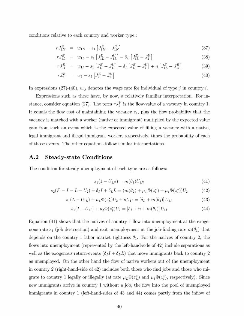
conditions relative to each country and worker type::

1 = 1 − 1

£1 −

1

¤(37)

1 = 1 − 1

£1 −

1

¤− £1 −

2

¤(38)

1 = 1 − 1

£1 −

1

¤− £1 −

2

¤+

£1 −

1

¤(39)

2 = 2 − 2

£2 −

2

¤(40)

In expressions (27)-(40), denotes the wage rate for individual of type in country .

Expressions such as these have, by now, a relatively familiar interpretation. For in-

stance, consider equation (27). The term 1 is the flow-value of a vacancy in country 1.

It equals the flow cost of maintaining the vacancy 1, plus the flow probability that the

vacancy is matched with a worker (native or immigrant) multiplied by the expected value

gain from such an event which is the expected value of filling a vacancy with a native,

legal immigrant and illegal immigrant worker, respectively, times the probability of each

of those events. The other equations follow similar interpretations.

A.2 Steady-state Conditions

The condition for steady unemployment of each type are as follows:

1(1− 1) = (1)1 (41)

2( − − − 2) + + = ((2) + Φ(∗) + Φ(

∗ ))2 (42)

1(− 1) + Φ(∗)2 + 1 = [ +(1)]1 (43)

1( − 1) + Φ(∗ )2 = [ + +(1)]1 (44)

Equation (41) shows that the natives of country 1 flow into unemployment at the exoge-

nous rate 1 (job destruction) and exit unemployment at the job-finding rate (1) that

depends on the country 1 labor market tightness 1. For the natives of country 2, the

flows into unemployment (represented by the left-hand-side of 42) include separations as

well as the exogenous return-events ( + ) that move immigrants back to country 2

as unemployed. On the other hand the flow of native workers out of the unemployment

in country 2 (right-hand-side of 42) includes both those who find jobs and those who mi-

grate to country 1 legally or illegally (at rate Φ(∗) and Φ(

∗ ), respectively). Since

new immigrants arrive in country 1 without a job, the flow into the pool of unemployed

immigrants in country 1 (left-hand-sides of 43 and 44) comes partly from the inflow of

40

new immigrants and partly from the job separations of incumbent immigrants. Flows into

the pool of legal unemployed immigrants (left-hand-side of 43) come also from incumbent

unemployed immigrants who switch from illegal to legal status (1). The flows of legal

immigrants out of unemployment (right-hand-side of 43) can be either due to job finding

or due to exogenous return to country 2. Similarly, flows of illegal immigrants out of un-

employment (right-hand-side of 44) come partly from job finding, (1)1 , partly from

returns, 1 and partly from legalizations, 1 .

Then equations (41) to (44) and equations (5) and (6) in the main text can be used

to derive expressions for the steady-state values of the unemployment rate and unem-

ployment level 1 1 1 and 2 for each group of workers (native, illegal and legal

immigrants in country 1 and natives in country 2):

1 = 1 =1

1 +(1)(45)

1 =1=

1 + +

1 + + +(1)(46)

1 =1=

1 + − (1− 1)

1 + +(1)(47)

2 =2

− − =

22 +(2)

(48)

where, consistently with the rest of the notation, () denote the unemployment level

(unemployment rate) in country = [1 2] of workers of type = [ ]. As it is

conventional, all unemployment rates increase with the relative separation probability

and decrease with the matching probability(). The unemployment rates of illegal and

legal immigrants, 1 and 1, increase also with the probability of exogenous return

and , respectively that in steady state act in a similar way as a separation rate. Return

rates in fact move workers out of employment in country 1 (as separation rates), and while

those workers flow to country 2, rather than to the unemployment pool of country 1, the

steady state conditions (5)-(6) ensure that there is an equal flow of migrants from country

2 to unemployment in country 1, hence reproducing the effect of separation. Notice that

while the legalization rate (as we will show below) increases the steady state value of

legal immigrants, and decreases the steady state number of illegal immigrants , it also

increases the unemployment rate among illegal 1 and decreases it among legal, 1. The

reason is that in steady state a higher flow out of illegal status (due to legalization) must

be balanced by a larger flow into it, which can only be provided by new illegal entry. As

41

those new illegal entrants are unemployed, the unemployment rate of that group rises.

Symmetrically for legal immigrants a higher legalization rate implies a larger flow into

the legalized pool and for a given flow out, this must be balanced by a lower flow of new

legal immigrants, with a decrease of unemployed new legal immigrants.

A.3 Wages

To understand the intuition behind the conditions that determine wages we can write

equations (9) to (12) in the text as follows:

1 = 1 + (1− )£1 +(1)(

1 −

1)¤

(49)

1 = 1 + (1− )£1 − +(1)(

1 −

1)¤

(50)

1 = 1 + (1− )£1 − +(1)(

1 −

1)¤

(51)

2 = 2 + (1− )£2 +(2)(

2 −

2 ) +¤

(52)

The term ≡ R ∗(∗−)Φ()+

R ∗(∗−)Φ(), in expression (52) measures the

expected gain of an immigration opportunity for a native of country 2. A worker’s wage

is a weighted average of the productivity of the match with a firm, , which only depends

on the country, and the outside option available to her (the term in the bracket). The

parameter expressing the workers’ bargaining power () is the weight put on productivity

by the Nash-bargaining formula. The outside options of the workers of country 1 depend

on their nativity and immigration status and they are equal to their unemployment flow

income plus the expected gain from search. The outside option of native workers of

country 2, instead, includes also the expected gain from a migration opportunity (either

legal or illegal) to country 1 (). Anything that improves the worker’s outside option will

also increase her wage, as it will improve her “threat point” in the wage setting process.

This explains why wages rise with the unemployment income and the matching rate

(), and in addition, fall with the search costs .18

18It should be noted that in expression (51) the probability of deportation , and the probability oflegalization affect wages only thought their impact on 1 − 1 . This is because we are assumingthat the probabilities of deportation and legalization are independent of employment status. It should

be noted that if we were to assume that illegal immigrants were more likely to become legal or that

their deportation probability was lower when employed than unemployed the wage expression (51) would

contain a term depending on those. In that case, immigrants would accept jobs at even lower wages,

because by so doing they could improve their chances of becoming legal or they would reduce their

deportation risk.

42

A.4 Immigration Cost Thresholds

Equations (13) and (14) in the text can be written in a more intuitive way as a function

of the endogenous wages:

(1− )∗ =[1 + (1− )1 − 1]− [2 − 2]

+ + (1− )(53)

(1− )∗ =[1 − 1]− [2 − 2]

+ (54)

where ≡ ++

. Expressions (53) and (54) make clear that the benefits from immigrat-

ing to country 1 increase when the wage that an immigrant worker can obtain in country

1 increases relative to the wage that she can obtain at home and when the return prob-

ability is small which implies that an immigrant worker’s stay in country 1 is expected

to last long. Essentially the terms in square brackets on the right hand side of equation

(53) are the flow value from being unemployed in country 1 for an illegal immigrant and

the flow value from unemployment in country 2. The difference depends positively on the

wage differential and also on the productivity differential (as the endogenous wages grow

faster than with an increase in ). Similarly the terms in square brackets on the right

hand side of (54) is the difference between the flow value from being unemployed as legal

immigrant in country 1 and being unemployed in country 2.

Since illegal immigrants may become legal with probability , their expected wage is a

weighted average of the wage they can get as illegal, 1 , and the wage they can get if they

become legal, 1, with the weight on 1 (1) increasing (decreasing) as the probability

of becoming legal () increases. Likewise, their return probability is a weighted average

of and , and the weight on is larger when is larger. The expected duration of

an immigrant’s stay in country 1 matters for incentives to enter into country 1, since, as

shown in the above equations, the effective discount rate for the benefits from entering

into country 1 is the discount rate plus the return probability , if entry is legal, and

the average return probability + (1− ) , if entry is illegal. Given that 1 1

and , an increase in implies an increase in the benefit from illegal entry and

therefore an increase in ∗ . By obtaining the legal status an immigrant worker can both

bargain for a higher wage and reduce his return probability, thus when the probability of

legalization increases the benefit from illegal entry also increases.

43

A.5 Value of a Filled Vacancy

Substituting the equilibrium wages (given in equations (9) to (12)) into equations (17) to

(20) the values of filled vacancies can be written as:

1 = (1− )1 =

(1− )(1 − 1)

+ 1 + (1)(55)

1 = (1− )1 =

(1− )(1 − 1 + )

+ 1 + + (1)(56)

1 = (1− )1 =

(1− ) (1 − 1 + ) + ¡1 −

1

¢ + 1 + + (1)

(57)

2 = (1− )2 =

(1− )(2 − 2 −)

+ 2 + (2)(58)

Obviously if = = 0 and = = 0, implying 1 = 1 = 1, then 1 =

1 =

1 and the firm is indifferent between hiring an immigrant (legal or illegal) or a

native worker. In general, however, the value of a filled job to the firm depends on the

worker’s origin and legal status, since as explained above, immigrants legal or illegal and

native workers earn different wages and in addition jobs filled by immigrants have lower

expected duration. More specifically, subtracting (56) from (55) and (57) from (56) gives

the two expressions (21) and (22) in the text.

44

45

Tables

Table 1

Parameterisation of the model =0.5 Petrongolo and Pissarides (2001). =0.5 Satisfies the Hosios (1990) condition. =0.004 Monthly interest rate.= =0.034 Hall (2005).

=1, z =0 Normalizations. Measured from the data:

=1 3⁄ The average ratio of Mexican to US population for the 2000s.*

=0.0023

Our calculations from several sources (see text).

=0.0039

Our calculations from several sources (see text).

=0.0006 Our calculations from several sources (See text).

Jointly calibrated to match:

=0.197 The employment rate of US-native workers: 0.82. †=0.053 The employment rate in Mexico: 0.55.† =0.262

The wage ratio between US and Mexico, equal to 4, close to the ratio of income per person in the two countries.‡

=0.672 =0.166

The ratio of unemployment to employment income of 71% for both countries (Hall and Milgrom, 2008).

=1.180 The native-immigrant wage gap: -25% (Borjas and Friedberg, 2009). =1.613

The legal-illegal immigrant wage gap: -10% (e.g. Rivera-Batiz, 1999 and Kossoudji and Cobb-Clark, 2012).

=0.412 The ratio of Mexican immigrants to the US-native labor force: + = 0.038. ⱡ =0.048

The proportion of legal immigrants in the total number of Mexican immigrants: 56% (Hoefer et al, 2012).

=0.0067% =0.035%

The vacancy to unemployment ratio in Mexico and the US: 0:620.¥

* http://www.oecd-ilibrary.org/statistics.** http://www.migrationinformation.org/DataHub/charts/fb-mexicans.cfm.† IPUMS Interna onal data. ‡ Penn World Table, version 7.1, available at: https://pwt.sas.upenn.edu/php site/pwt index.php. ⱡ IPUMS in 2000. ¥ Conference Board's Help-Wanted Index.

46

Table 2: Higher search cost (increase in ) (percentage changes)

-15% native-immigrant wage gap

-5% legal-illegal wage gap

Double Reduce the ratio of unemployment to employment income to 0.5

-10 -50 -10 -50 -10 -50 -10 -50 7,69 28,71 3,00 11,56 1,92 7,50 1,88 7,31

-0,20 -1,45 -0,68 -3,18 -0,72 -3,26 -0,47 -2,12

0,08 0,60 0,28 1,30 0,30 1,33 0,19 0,87 0,16 0,94 0,35 1,64 0,37 1,66 0,27 1,22 0,08 0,58 0,27 1,27 0,29 1,30 0,19 0,85

0,00 -0,03 -0,01 -0,06 -0,01 -0,06 -0,02 -0,07 -0,01 -0,09 -0,08 -0,40 -0,08 -0,37 -0,06 -0,28 -2,11 -9,18 -1,29 -5,44 -0,97 -4,04 -0,92 -3,77

-0,01 -0,07 -0,03 -0,14 -0,03 -0,14 -0,04 -0,17 -0,02 -0,17 -0,08 -0,36 -0,08 -0,37 -0,06 -0,28

⋆ -9,58 -48,91 -10,15 -50,92 -10,18 -50,98 -10,47 -52,04⋆ 0,15 0,36 -0,29 -1,61 -0,29 -1,46 -0,21 -1,11 -2,19 -9,04 -2,08 -9,01 -1,08 -4,57 -1,76 -7,60 0,21 0,88 0,21 0,88 0,19 0,80 0,21 0,85 3,51 16,70 3,56 16,71 3,88 17,72 3,69 17,21

L/(L+I+1) -1,99 -8,23 -1,89 -8,19 -0,91 -3,85 -1,57 -6,81(L+I) /(L+I+1) -5,35 -24,23 -5,29 -24,21 -4,73 -21,36 -5,12 -23,31

4,03 13,95 1,96 6,80 1,58 5,57 0,71 2,46 -1,11 -3,90 -0,54 -1,88 -0,44 -1,54 -0,20 -0,68 -0,19 -0,68 -0,11 -0,40 -0,09 -0,31 -0,08 -0,27 0,75 3,01 0,70 2,87 0,63 2,58 0,67 2,75 1,42 5,29 1,02 3,97 0,89 3,49 0,75 3,03

47

Table 3: Increased rates of deportation (increase in ) (percentage changes)

-15% native-immigrant wage gap

-5% legal-illegal wage gap

Double Reduce the ratio of unemployment to employment income to 0.5

-10 -50 -10 -50 -10 -50 -10 -50 6,96 33,30 6,04 28,80 5,37 25,58 5,44 25,59

-0,63 -2,66 -0,88 -3,74 -0,86 -3,62 -0,56 -2,34

0,26 1,09 0,36 1,53 0,35 1,48 0,23 0,96 0,34 1,44 0,44 1,87 0,43 1,81 0,31 1,31 0,83 4,19 0,86 4,14 0,79 3,76 0,67 3,26

-0,01 -0,05 -0,02 -0,07 -0,02 -0,07 -0,02 -0,08 -0,04 -0,17 -0,11 -0,47 -0,10 -0,41 -0,07 -0,31 -0,21 -1,07 -0,31 -1,52 -0,32 -1,52 -0,30 -1,46

-0,03 -0,12 -0,04 -0,16 -0,04 -0,16 -0,04 -0,18 -0,07 -0,30 -0,10 -0,43 -0,10 -0,41 -0,07 -0,31

⋆ -4,09 -21,07 -5,13 -26,13 -5,66 -28,84 -5,81 -29,70⋆ -0,05 -0,21 -0,53 -2,30 -0,42 -1,83 -0,33 -1,41 -1,89 -8,14 -2,10 -9,07 -1,06 -4,54 -1,80 -7,70 0,20 0,83 0,20 0,85 0,18 0,77 0,20 0,83 3,39 15,91 3,33 15,75 3,70 16,95 3,49 16,35

L/(L+I+1) -1,70 -7,34 -1,90 -8,25 -0,89 -3,82 -1,61 -6,91(L+I) /(L+I+1) -5,19 -23,65 -5,30 -24,24 -4,72 -21,34 -5,13 -23,37

1,89 8,05 1,12 4,61 1,02 4,16 0,44 1,78 -0,52 -2,23 -0,31 -1,28 -0,28 -1,15 -0,12 -0,49 -0,09 -0,39 -0,06 -0,27 -0,06 -0,23 -0,05 -0,20 0,70 2,87 0,70 2,86 0,63 2,56 0,67 2,75 1,02 4,20 0,88 3,61 0,79 3,24 0,72 2,95

48

Table 4: Increased border control (entry restrictions) (decrease in ) (percentage changes)

-15% native-immigrant wage gap

-5% legal-illegal wage gap

Double Reduce the ratio of unemployment to employment income to 0.5

-10 -50 -10 -50 -10 -50 -10 -50 -9,87 -49,47 -9,40 -47,36 -8,94 -45,34 -9,47 -47,59

-0,65 -2,72 -0,90 -3,81 -0,87 -3,69 -0,57 -2,37

0,27 1,11 0,37 1,56 0,36 1,51 0,23 0,97 0,34 1,46 0,45 1,90 0,44 1,84 0,31 1,32 0,26 1,09 0,36 1,52 0,35 1,47 0,23 0,95

-0,01 -0,05 -0,02 -0,07 -0,02 -0,07 -0,02 -0,08 -0,04 -0,17 -0,11 -0,48 -0,10 -0,42 -0,07 -0,31 -0,07 -0,29 -0,14 -0,58 -0,15 -0,62 -0,11 -0,45

-0,03 -0,12 -0,04 -0,17 -0,04 -0,16 -0,04 -0,19 -0,07 -0,31 -0,10 -0,44 -0,10 -0,42 -0,07 -0,31

⋆ -0,17 -0,72 -0,95 -4,13 -1,38 -6,03 -1,08 -4,66⋆ -0,04 -0,16 -0,54 -2,33 -0,43 -1,86 -0,34 -1,45 -1,97 -8,38 -2,12 -9,14 -1,08 -4,58 -1,80 -7,72 0,21 0,87 0,21 0,88 0,19 0,80 0,21 0,85 3,61 16,93 3,54 16,67 3,88 17,71 3,68 17,17

L/(L+I+1) -1,77 -7,58 -1,92 -8,32 -0,90 -3,85 -1,61 -6,93(L+I) /(L+I+1) -5,23 -23,81 -5,31 -24,29 -4,73 -21,36 -5,14 -23,38

2,31 9,26 1,22 4,82 1,05 4,16 0,44 1,73 -0,64 -2,57 -0,33 -1,33 -0,29 -1,15 -0,12 -0,48 -0,11 -0,45 -0,07 -0,28 -0,06 -0,23 -0,05 -0,19 0,71 2,90 0,70 2,86 0,63 2,57 0,67 2,75 1,10 4,43 0,90 3,64 0,80 3,25 0,72 2,95

49

Table 5: Legalization (increase in ) (percentage changes)

-15% native-immigrant wage gap

-5% legal-illegal wage gap

Double Reduce the ratio of unemployment to employment income to 0.5

-10 -50 -10 -50 -10 -50 -10 -50 87,26 227,79 90,10 229,45 95,48 237,52 164,85 282,46

0,40 1,71 1,32 5,18 0,25 0,96 2,84 6,10

-0,16 -0,70 -0,54 -2,13 -0,10 -0,39 -1,17 -2,51 -0,95 -2,69 -1,35 -4,12 -1,15 -3,44 -2,93 -5,09 1,56 9,44 1,28 8,26 1,87 10,80 3,92 14,94

0,01 0,03 0,03 0,10 0,00 0,02 0,09 0,20 0,02 0,11 0,16 0,64 0,03 0,11 0,37 0,80 -0,10 -0,68 0,13 0,40 -0,15 -0,97 0,12 -0,33

0,02 0,08 0,06 0,23 0,01 0,04 0,23 0,49 0,05 0,20 0,15 0,59 0,03 0,11 0,38 0,81

⋆ 7,20 27,50 8,52 31,00 9,32 33,09 38,17 71,90⋆ -0,08 -0,45 0,74 2,73 0,00 -0,12 1,26 2,13 21,26 69,47 22,47 70,75 12,96 44,91 55,39 104,48 -0,34 -1,46 -0,38 -1,52 -0,15 -0,59 -1,42 -3,23 12,05 35,52 12,47 35,75 8,33 28,06 22,48 40,93

L/(L+I+1) 20,93 68,06 22,11 69,29 12,83 44,38 54,04 101,38(L+I) /(L+I+1) 8,36 31,42 9,10 32,40 3,37 12,95 30,31 58,90

-3,71 -18,52 -2,10 -9,88 -1,65 -7,68 -4,40 -12,55 1,02 4,99 0,58 2,69 0,45 2,09 1,20 3,40 0,17 0,83 0,12 0,55 0,09 0,41 0,47 1,32 -1,24 -5,47 -1,31 -5,44 -0,48 -1,98 -4,98 -11,94 -1,86 -8,67 -1,65 -7,09 -0,75 -3,26 -5,49 -13,43

50

Table 6: Take it or leave it offer, Higher search cost (increase in ) (percentage changes)

-10 -20 -30 -40 -50 -60 -70 -80 -90 593.69 659.20 695.90 720.76 739.11 753.34 764.74 774.08 781.86

0.29 0.35 0.23 -0.03 -0.39 -0.83 -1.32 -1.84 -2.38

-0.12 -0.14 -0.10 0.01 0.16 0.34 0.54 0.75 0.97 -0.04 0.01 0.13 0.30 0.51 0.74 0.99 1.25 1.51 -0.12 -0.14 -0.09 0.01 0.16 0.33 0.53 0.74 0.95

0.01 0.01 0.00 0.00 -0.01 -0.02 -0.03 -0.04 -0.05 0.03 0.04 0.03 0.00 -0.05 -0.10 -0.15 -0.21 -0.27 -6.77 -13.49 -20.12 -26.63 -32.98 -39.14 -45.11 -50.85 -56.37

0.01 0.01 0.01 -0.01 -0.02 -0.04 -0.06 -0.08 -0.11 0.03 0.04 0.02 -0.01 -0.05 -0.10 -0.16 -0.22 -0.28

⋆ -9.13 -18.46 -27.95 -37.57 -47.29 -57.10 -66.97 -76.90 -86.86⋆ 0.64 1.06 1.30 1.41 1.41 1.32 1.17 0.98 0.75 -2.15 -4.18 -6.08 -7.87 -9.53 -11.08 -12.53 -13.88 -15.13 0.21 0.41 0.58 0.74 0.89 1.02 1.14 1.25 1.35 3.52 6.94 10.25 13.45 16.52 19.47 22.29 24.97 27.53

L/(L+I+1) -1.96 -3.81 -5.54 -7.18 -8.71 -10.14 -11.47 -12.72 -13.88(L+I) /(L+I+1) -5.33 -10.46 -15.37 -20.07 -24.54 -28.80 -32.83 -36.65 -40.26

5.62 10.24 14.04 17.17 19.73 21.85 23.59 25.02 26.20 -1.56 -2.85 -3.92 -4.81 -5.55 -6.15 -6.66 -7.07 -7.42 -0.26 -0.49 -0.68 -0.83 -0.97 -1.08 -1.17 -1.24 -1.31 0.78 1.47 2.08 2.62 3.11 3.55 3.94 4.29 4.61 1.71 3.15 4.37 5.41 6.31 7.07 7.73 8.31 8.81

51

Table 7: Take it or leave it offer, Enforcement of deportation (increase in ) (percentage changes)

-10 -20 -30 -40 -50 -60 -70 -80 -90 7.55 14.93 22.16 29.25 36.20 43.04 49.76 56.38 62.91

-0.92 -1.76 -2.53 -3.23 -3.87 -4.46 -5.00 -5.48 -5.93

0.38 0.72 1.04 1.32 1.59 1.83 2.04 2.24 2.42 0.45 0.87 1.25 1.60 1.92 2.22 2.49 2.73 2.96 1.00 2.00 2.99 3.98 4.98 5.99 7.00 8.03 9.08

-0.02 -0.03 -0.05 -0.06 -0.07 -0.09 -0.10 -0.11 -0.11 -0.11 -0.20 -0.29 -0.37 -0.45 -0.51 -0.58 -0.63 -0.68 0.00 0.00 0.00 -0.01 -0.01 -0.01 -0.01 -0.01 -0.01

-0.04 -0.08 -0.12 -0.15 -0.18 -0.21 -0.23 -0.26 -0.28 -0.11 -0.21 -0.30 -0.38 -0.46 -0.53 -0.59 -0.65 -0.70

⋆ -3.45 -6.95 -10.52 -14.15 -17.84 -21.58 -25.38 -29.23 -33.13⋆ -0.38 -0.72 -1.04 -1.32 -1.57 -1.80 -2.01 -2.19 -2.36 -2.26 -4.37 -6.33 -8.15 -9.85 -11.42 -12.87 -14.21 -15.45 0.21 0.39 0.56 0.72 0.86 0.99 1.11 1.21 1.31 3.20 6.33 9.37 12.32 15.17 17.92 20.56 23.09 25.51

L/(L+I+1) -2.06 -3.99 -5.78 -7.46 -9.02 -10.47 -11.81 -13.05 -14.19(L+I) /(L+I+1) -5.39 -10.57 -15.52 -20.24 -24.74 -29.02 -33.06 -36.89 -40.49

2.44 4.72 6.83 8.80 10.63 12.33 13.90 15.36 16.71 -0.67 -1.30 -1.89 -2.44 -2.96 -3.44 -3.88 -4.30 -4.68 -0.11 -0.22 -0.32 -0.42 -0.51 -0.59 -0.67 -0.74 -0.81 0.74 1.40 2.00 2.53 3.02 3.46 3.85 4.21 4.53 1.14 2.18 3.13 3.99 4.77 5.48 6.13 6.72 7.25

52

Table 8: Take it or leave it offer , Restrictions on entry (decrease in ) (percentage changes)

-10 -20 -30 -40 -50 -60 -70 -80 -90 -9.92 -19.86 -29.80 -39.75 -49.71 -59.67 -69.64 -79.61 -89.58

-0.98 -1.87 -2.69 -3.43 -4.10 -4.71 -5.26 -5.77 -6.22

0.40 0.77 1.10 1.40 1.68 1.93 2.15 2.36 2.54 0.47 0.91 1.31 1.67 2.00 2.31 2.58 2.83 3.06 0.39 0.75 1.07 1.37 1.64 1.88 2.10 2.30 2.48

-0.02 -0.04 -0.05 -0.07 -0.08 -0.09 -0.10 -0.11 -0.12 -0.11 -0.21 -0.31 -0.39 -0.47 -0.54 -0.61 -0.67 -0.72 0.00 0.00 -0.01 -0.01 -0.01 -0.01 -0.01 -0.01 -0.01

-0.04 -0.08 -0.12 -0.15 -0.18 -0.20 -0.23 -0.25 -0.27 -0.11 -0.21 -0.31 -0.39 -0.47 -0.54 -0.60 -0.66 -0.71

⋆ 0.13 0.25 0.36 0.45 0.54 0.62 0.69 0.75 0.81⋆ -0.35 -0.67 -0.96 -1.23 -1.48 -1.70 -1.91 -2.10 -2.27 -2.42 -4.66 -6.73 -8.64 -10.40 -12.02 -13.51 -14.88 -16.13 0.22 0.42 0.60 0.76 0.91 1.04 1.16 1.27 1.37 3.41 6.75 10.00 13.16 16.21 19.15 21.98 24.68 27.25

L/(L+I+1) -2.22 -4.27 -6.18 -7.94 -9.56 -11.06 -12.44 -13.70 -14.86(L+I) /(L+I+1) -5.48 -10.74 -15.76 -20.54 -25.10 -29.41 -33.49 -37.35 -40.97

3.32 6.27 8.91 11.26 13.36 15.24 16.92 18.43 19.79 -0.92 -1.74 -2.47 -3.13 -3.73 -4.26 -4.74 -5.17 -5.56 -0.16 -0.30 -0.42 -0.54 -0.64 -0.74 -0.82 -0.90 -0.97 0.76 1.44 2.05 2.60 3.09 3.53 3.93 4.28 4.60 1.31 2.48 3.52 4.45 5.28 6.02 6.68 7.28 7.81

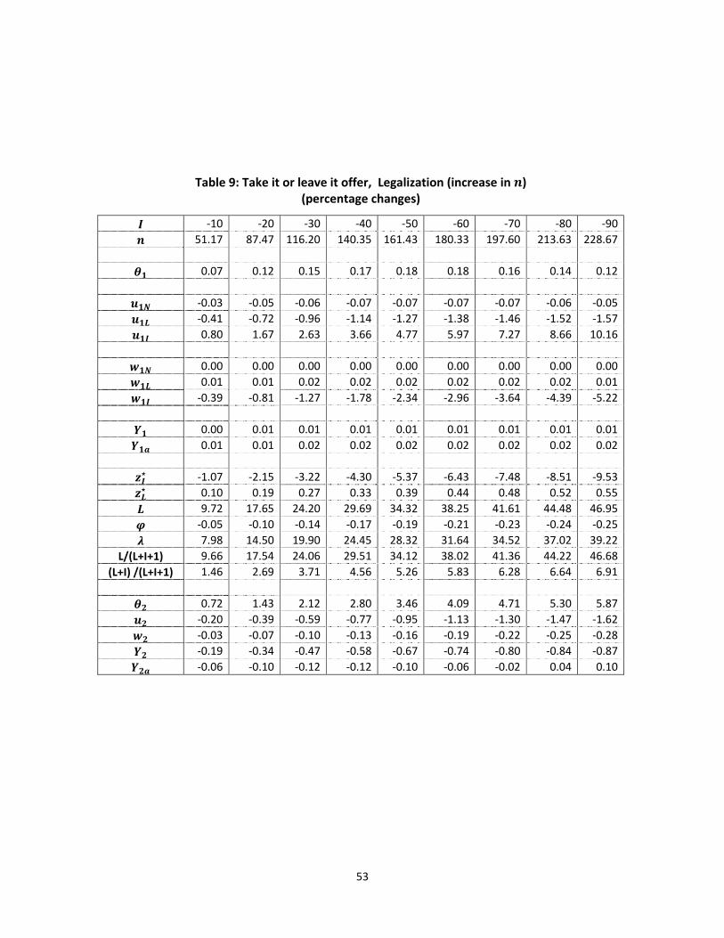
53

Table 9: Take it or leave it offer, Legalization (increase in ) (percentage changes)

-10 -20 -30 -40 -50 -60 -70 -80 -90 51.17 87.47 116.20 140.35 161.43 180.33 197.60 213.63 228.67

0.07 0.12 0.15 0.17 0.18 0.18 0.16 0.14 0.12

-0.03 -0.05 -0.06 -0.07 -0.07 -0.07 -0.07 -0.06 -0.05 -0.41 -0.72 -0.96 -1.14 -1.27 -1.38 -1.46 -1.52 -1.57 0.80 1.67 2.63 3.66 4.77 5.97 7.27 8.66 10.16

0.00 0.00 0.00 0.00 0.00 0.00 0.00 0.00 0.00 0.01 0.01 0.02 0.02 0.02 0.02 0.02 0.02 0.01 -0.39 -0.81 -1.27 -1.78 -2.34 -2.96 -3.64 -4.39 -5.22

0.00 0.01 0.01 0.01 0.01 0.01 0.01 0.01 0.01 0.01 0.01 0.02 0.02 0.02 0.02 0.02 0.02 0.02

⋆ -1.07 -2.15 -3.22 -4.30 -5.37 -6.43 -7.48 -8.51 -9.53⋆ 0.10 0.19 0.27 0.33 0.39 0.44 0.48 0.52 0.55 9.72 17.65 24.20 29.69 34.32 38.25 41.61 44.48 46.95 -0.05 -0.10 -0.14 -0.17 -0.19 -0.21 -0.23 -0.24 -0.25 7.98 14.50 19.90 24.45 28.32 31.64 34.52 37.02 39.22

L/(L+I+1) 9.66 17.54 24.06 29.51 34.12 38.02 41.36 44.22 46.68(L+I) /(L+I+1) 1.46 2.69 3.71 4.56 5.26 5.83 6.28 6.64 6.91

0.72 1.43 2.12 2.80 3.46 4.09 4.71 5.30 5.87 -0.20 -0.39 -0.59 -0.77 -0.95 -1.13 -1.30 -1.47 -1.62 -0.03 -0.07 -0.10 -0.13 -0.16 -0.19 -0.22 -0.25 -0.28 -0.19 -0.34 -0.47 -0.58 -0.67 -0.74 -0.80 -0.84 -0.87 -0.06 -0.10 -0.12 -0.12 -0.10 -0.06 -0.02 0.04 0.10

54

Figures

-100-90-80-70-60-50-40-30-20-100-10

-5

0

5

10

15

% change in I

% c

hang

e in

mar

ket t

ight

ness

Figure 1: Effects on market tightness

search costdeportationrestrict entrylegalization

-100-90-80-70-60-50-40-30-20-100-6

-5

-4

-3

-2

-1

0

1

2

3

% change in I

% c

hang

e in

the

unem

ploy

men

rate

of n

ativ

es

Figure 2: Effects on the unemployment rate of natives

search costdeportationrestrict entrylegalization

55

-100-90-80-70-60-50-40-30-20-100-0.15

-0.1

-0.05

0

0.05

0.1

0.15

0.2

0.25

% change in I

% c

hang

e in

the

wag

e of

nat

ives

Figure 3: Effects on the wage of natives

search costdeportationrestrict entrylegalization

-100-90-80-70-60-50-40-30-20-100-1

-0.5

0

0.5

1

1.5

% change in I

% c

hang

e in

the

wag

e of

lega

l im

mig

rant

s

Figure 4: Effects on the wage of legal immigrants

search costdeportationrestrict entrylegalization

56

-100-90-80-70-60-50-40-30-20-100-7

-6

-5

-4

-3

-2

-1

0

1

% change in I

% c

hang

e in

the

wag

e of

ille

gal i

mm

igra

nts

Figure 5: Effects on the wage of illegal immigrants

search costdeportationrestrict entrylegalization

-100-90-80-70-60-50-40-30-20-100-0.3

-0.2

-0.1

0

0.1

0.2

0.3

0.4

0.5

0.6

% change in I

% c

hang

e in

the

net i

ncom

e of

nat

ives

Figure 6: Effects on the net income of native workers

search costdeportationrestrict entrylegalization

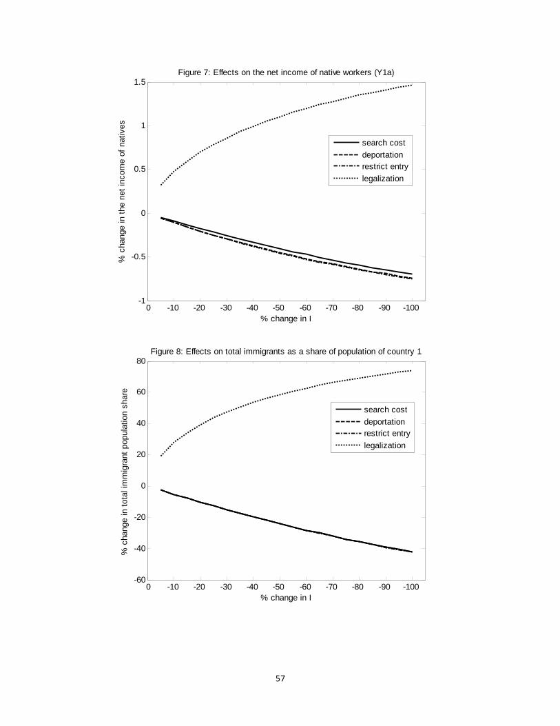
57

-100-90-80-70-60-50-40-30-20-100-1

-0.5

0

0.5

1

1.5

% change in I

% c

hang

e in

the

net i

ncom

e of

nat

ives

Figure 7: Effects on the net income of native workers (Y1a)

search costdeportationrestrict entrylegalization

-100-90-80-70-60-50-40-30-20-100-60

-40

-20

0

20

40

60

80

% change in I

% c

hang

e in

tota

l im

mig

rant

pop

ulat

ion

shar

e

Figure 8: Effects on total immigrants as a share of population of country 1

search costdeportationrestrict entrylegalization

58

-100-90-80-70-60-50-40-30-20-100-20

0

20

40

60

80

100

120

140

% change in I

% c

hang

e in

lega

l im

mig

rant

pop

ulat

ion

shar

e

Figure 9: Effects on legal immigrants as a share of population of country 1

search costdeportationrestrict entrylegalization

59

Appendix of Tables

Table A1: Higher search cost (increase in ) (percentage changes)

-5 -10 -15 -20 -25 -30 -35 -40 -45 -50 1,06 2,05 2,98 3,84 4,64 5,40 6,10 6,76 7,37 7,95

Country 1

-0,39 -0,78 -1,16 -1,53 -1,89 -2,24 -2,58 -2,91 -3,23 -3,54Unemployment rates

0,16 0,32 0,48 0,63 0,77 0,92 1,06 1,19 1,32 1,45 0,20 0,40 0,59 0,78 0,96 1,14 1,31 1,47 1,63 1,79 0,16 0,31 0,46 0,61 0,76 0,90 1,03 1,16 1,29 1,42

Wages -0,01 -0,01 -0,02 -0,03 -0,04 -0,04 -0,05 -0,06 -0,06 -0,07 -0,05 -0,09 -0,13 -0,18 -0,22 -0,26 -0,30 -0,33 -0,37 -0,41 -0,53 -1,04 -1,52 -1,98 -2,42 -2,84 -3,24 -3,62 -3,98 -4,32

Net output -0,02 -0,03 -0,05 -0,07 -0,08 -0,10 -0,11 -0,13 -0,14 -0,15 -0,04 -0,09 -0,13 -0,17 -0,22 -0,26 -0,29 -0,33 -0,37 -0,40

Legal immigration and composition ⋆ -5,13 -10,26 -15,39 -20,52 -25,65 -30,79 -35,92 -41,05 -46,18 -51,31⋆ -0,16 -0,33 -0,50 -0,67 -0,83 -1,00 -1,17 -1,33 -1,50 -1,66 -1,03 -2,03 -2,98 -3,90 -4,79 -5,64 -6,45 -7,24 -7,99 -8,71 0,11 0,21 0,31 0,40 0,49 0,58 0,66 0,73 0,81 0,87 1,80 3,58 5,33 7,06 8,76 10,43 12,08 13,69 15,27 16,82

Country 2 0,81 1,54 2,20 2,80 3,34 3,83 4,27 4,67 5,04 5,37 -0,22 -0,42 -0,61 -0,77 -0,92 -1,06 -1,18 -1,29 -1,39 -1,48 -0,05 -0,09 -0,13 -0,16 -0,20 -0,22 -0,25 -0,27 -0,30 -0,32 0,36 0,70 1,02 1,32 1,61 1,88 2,14 2,39 2,62 2,84 0,49 0,95 1,38 1,78 2,15 2,50 2,83 3,14 3,43 3,71

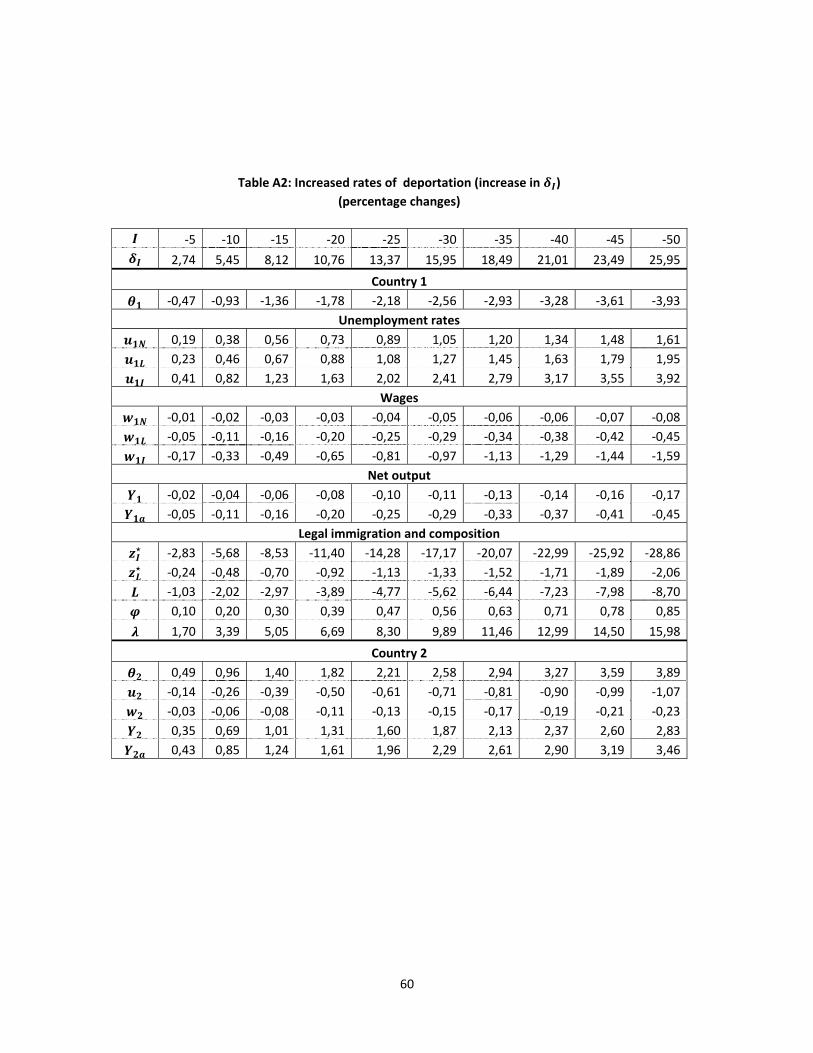
60

Table A2: Increased rates of deportation (increase in ) (percentage changes)

-5 -10 -15 -20 -25 -30 -35 -40 -45 -50 2,74 5,45 8,12 10,76 13,37 15,95 18,49 21,01 23,49 25,95

Country 1 -0,47 -0,93 -1,36 -1,78 -2,18 -2,56 -2,93 -3,28 -3,61 -3,93

Unemployment rates 0,19 0,38 0,56 0,73 0,89 1,05 1,20 1,34 1,48 1,61 0,23 0,46 0,67 0,88 1,08 1,27 1,45 1,63 1,79 1,95 0,41 0,82 1,23 1,63 2,02 2,41 2,79 3,17 3,55 3,92

Wages -0,01 -0,02 -0,03 -0,03 -0,04 -0,05 -0,06 -0,06 -0,07 -0,08 -0,05 -0,11 -0,16 -0,20 -0,25 -0,29 -0,34 -0,38 -0,42 -0,45 -0,17 -0,33 -0,49 -0,65 -0,81 -0,97 -1,13 -1,29 -1,44 -1,59

Net output -0,02 -0,04 -0,06 -0,08 -0,10 -0,11 -0,13 -0,14 -0,16 -0,17 -0,05 -0,11 -0,16 -0,20 -0,25 -0,29 -0,33 -0,37 -0,41 -0,45

Legal immigration and composition ⋆ -2,83 -5,68 -8,53 -11,40 -14,28 -17,17 -20,07 -22,99 -25,92 -28,86⋆ -0,24 -0,48 -0,70 -0,92 -1,13 -1,33 -1,52 -1,71 -1,89 -2,06 -1,03 -2,02 -2,97 -3,89 -4,77 -5,62 -6,44 -7,23 -7,98 -8,70 0,10 0,20 0,30 0,39 0,47 0,56 0,63 0,71 0,78 0,85 1,70 3,39 5,05 6,69 8,30 9,89 11,46 12,99 14,50 15,98

Country 2 0,49 0,96 1,40 1,82 2,21 2,58 2,94 3,27 3,59 3,89 -0,14 -0,26 -0,39 -0,50 -0,61 -0,71 -0,81 -0,90 -0,99 -1,07 -0,03 -0,06 -0,08 -0,11 -0,13 -0,15 -0,17 -0,19 -0,21 -0,23 0,35 0,69 1,01 1,31 1,60 1,87 2,13 2,37 2,60 2,83 0,43 0,85 1,24 1,61 1,96 2,29 2,61 2,90 3,19 3,46

61

Table A3: Increased border control (entry restrictions) (decrease in ) (percentage changes)

-5 -10 -15 -20 -25 -30 -35 -40 -45 -50 -4,47 -8,96 -13,47 -17,98 -22,51 -27,06 -31,62 -36,20 -40,79 -45,39

Country 1 -0,48 -0,95 -1,39 -1,81 -2,22 -2,61 -2,98 -3,33 -3,67 -4,00

Unemployment rates 0,20 0,39 0,57 0,74 0,91 1,07 1,22 1,37 1,50 1,64 0,24 0,46 0,68 0,89 1,09 1,28 1,47 1,64 1,81 1,97 0,19 0,38 0,56 0,73 0,89 1,04 1,19 1,33 1,47 1,60

Wages -0,01 -0,02 -0,03 -0,03 -0,04 -0,05 -0,06 -0,06 -0,07 -0,08 -0,06 -0,11 -0,16 -0,21 -0,25 -0,30 -0,34 -0,38 -0,42 -0,46 -0,08 -0,16 -0,23 -0,31 -0,37 -0,44 -0,50 -0,56 -0,62 -0,68

Net output -0,02 -0,04 -0,06 -0,08 -0,10 -0,11 -0,13 -0,14 -0,16 -0,17 -0,05 -0,11 -0,16 -0,21 -0,25 -0,30 -0,34 -0,38 -0,42 -0,46

Legal immigration and composition ⋆ -0,73 -1,44 -2,13 -2,80 -3,44 -4,06 -4,66 -5,23 -5,79 -6,32⋆ -0,25 -0,48 -0,71 -0,94 -1,15 -1,35 -1,55 -1,74 -1,92 -2,09 -1,04 -2,03 -2,99 -3,91 -4,80 -5,65 -6,47 -7,26 -8,02 -8,74 0,11 0,21 0,31 0,40 0,49 0,58 0,66 0,73 0,81 0,88 1,80 3,58 5,33 7,06 8,76 10,43 12,07 13,68 15,26 16,81

Country 2 0,51 0,99 1,45 1,87 2,26 2,64 2,98 3,31 3,62 3,91 -0,14 -0,27 -0,40 -0,51 -0,62 -0,73 -0,82 -0,91 -1,00 -1,08 -0,03 -0,06 -0,08 -0,11 -0,13 -0,15 -0,17 -0,19 -0,21 -0,23 0,35 0,69 1,01 1,31 1,60 1,87 2,13 2,37 2,61 2,83 0,44 0,85 1,25 1,62 1,97 2,30 2,62 2,91 3,20 3,46

62

Table A4: Legalization (increase in ) (percentage changes)

-5 -10 -15 -20 -25 -30 -35 -40 -45 -50 119,11 156,69 182,16 202,13 218,88 233,52 246,65 258,64 269,75 280,15

Country 1 2,82 4,21 5,28 6,17 6,95 7,63 8,25 8,81 9,32 9,79

Unemployment rates -1,16 -1,73 -2,17 -2,54 -2,86 -3,14 -3,39 -3,63 -3,84 -4,03 -2,38 -3,37 -4,05 -4,60 -5,04 -5,42 -5,76 -6,05 -6,31 -6,54 1,68 2,90 4,08 5,27 6,49 7,74 9,03 10,36 11,73 13,15

Wages 0,05 0,08 0,10 0,12 0,13 0,15 0,16 0,17 0,18 0,19 0,32 0,48 0,60 0,70 0,79 0,86 0,93 1,00 1,05 1,11 0,24 0,33 0,38 0,40 0,40 0,38 0,35 0,31 0,26 0,20

Net output 0,12 0,18 0,23 0,27 0,31 0,34 0,36 0,39 0,41 0,43 0,32 0,48 0,60 0,70 0,79 0,86 0,93 0,99 1,05 1,10

Legal immigration and composition ⋆ 23,16 33,16 40,31 45,98 50,70 54,75 58,29 61,42 64,23 66,76⋆ 1,23 1,78 2,17 2,48 2,74 2,95 3,13 3,29 3,43 3,55 36,07 51,88 63,17 72,06 79,43 85,71 91,16 95,97 100,26 104,11 -0,85 -1,29 -1,64 -1,94 -2,20 -2,44 -2,66 -2,86 -3,04 -3,21 15,15 21,54 25,98 29,38 32,14 34,44 36,41 38,11 39,60 40,92

Country 2 -5,07 -8,15 -10,80 -13,22 -15,50 -17,65 -19,71 -21,69 -23,59 -25,42 1,39 2,22 2,93 3,58 4,19 4,76 5,30 5,82 6,31 6,79 0,29 0,46 0,61 0,74 0,86 0,98 1,08 1,19 1,28 1,38 -2,95 -4,55 -5,85 -6,97 -7,98 -8,90 -9,75 -10,54 -11,28 -11,98 -3,79 -5,90 -7,65 -9,18 -10,58 -11,87 -13,09 -14,22 -15,30 -16,33

63

Table A5: Legalization and increased border control (increase in and decrease in ) (percentage changes)

-10 -20 -30 -40 -50 -60 -70 -80 -90 -100 41,44 73,27 99,60 122,38 142,67 161,15 178,24 194,24 209,38 223,81 -8,46 -16,64 -24,51 -32,06 -39,28 -46,17 -52,72 -58,94 -64,82 -70,37

Country 1 -0,22 -0,43 -0,61 -0,78 -0,93 -1,07 -1,19 -1,31 -1,41 -1,50

Unemployment rates 0,09 0,18 0,25 0,32 0,38 0,44 0,49 0,54 0,58 0,62 -0,20 -0,34 -0,44 -0,52 -0,58 -0,63 -0,66 -0,68 -0,70 -0,71 0,73 1,51 2,34 3,24 4,21 5,25 6,37 7,58 8,89 10,29

Wages 0,00 -0,01 -0,01 -0,01 -0,02 -0,02 -0,02 -0,03 -0,03 -0,03 -0,03 -0,05 -0,07 -0,09 -0,11 -0,12 -0,14 -0,15 -0,16 -0,17 -0,09 -0,18 -0,27 -0,37 -0,47 -0,58 -0,69 -0,81 -0,94 -1,07

Net output -0,01 -0,02 -0,03 -0,03 -0,04 -0,04 -0,05 -0,05 -0,06 -0,06 -0,03 -0,05 -0,07 -0,09 -0,10 -0,12 -0,13 -0,15 -0,16 -0,17

Legal immigration and composition ⋆ 5,06 10,04 14,92 19,68 24,31 28,78 33,09 37,22 41,18 44,95⋆ -0,15 -0,28 -0,41 -0,53 -0,64 -0,74 -0,83 -0,92 -1,00 -1,08 7,21 13,32 18,54 23,03 26,94 30,34 33,33 35,95 38,27 40,32 0,01 0,01 0,02 0,02 0,02 0,03 0,03 0,03 0,04 0,04 7,07 13,09 18,25 22,71 26,59 29,99 32,97 35,60 37,93 40,00

L/(L+I+1) 7,21 13,32 18,54 23,03 26,94 30,34 33,33 35,95 38,27 40,32(L+I) /(L+I+1) 0,00 0,00 0,00 0,00 0,00 0,00 0,00 0,00 0,00 0,00

Country 2 -0,10 -0,22 -0,34 -0,49 -0,64 -0,80 -0,96 -1,14 -1,31 -1,49 0,03 0,06 0,09 0,13 0,18 0,22 0,26 0,31 0,36 0,41 0,01 0,01 0,02 0,03 0,04 0,05 0,06 0,07 0,08 0,09 0,00 0,00 0,00 0,00 -0,01 -0,01 -0,01 -0,01 -0,01 -0,02 -0,02 -0,04 -0,06 -0,08 -0,11 -0,14 -0,17 -0,20 -0,23 -0,26