Embed Size (px)
Citation preview
The Knowledge Graph for Macroeconomic Analysis
with Alternative Big Data
Yucheng Yang Yue Pang Guanhua Huang Weinan E∗
October 2020
Abstract
The current knowledge system of macroeconomics is built on interactions among a small number of
variables, since traditional macroeconomic models can mostly handle a handful of inputs. Recent work
using big data suggests that a much larger number of variables are active in driving the dynamics of the
aggregate economy. In this paper, we introduce a knowledge graph (KG) that consists of not only linkages
between traditional economic variables but also new alternative big data variables. We extract these new
variables and the linkages by applying advanced natural language processing (NLP) tools on the massive
textual data of academic literature and research reports. As one example of the potential applications, we
use it as the prior knowledge to select variables for economic forecasting models in macroeconomics. Com-
pared to statistical variable selection methods, KG-based methods achieve significantly higher forecasting
accuracy, especially for long run forecasts.
Keywords: Big Data, Alternative/Nontraditional Data, Knowledge Graph, Natural Language Processing,
Variable Selection, Economic Forecasting.
∗Yucheng Yang and Weinan E: Princeton University. Yue Pang: Peking University. Guanhua Huang: University of Scienceand Technology China. We thank Feng Lu, Chris Sims, Yi Zhang, Lei Zou and audience in the BIBDR Economics and Big DataWorkshop for helpful comments, and thank Hanrong Liu, Tao Wen and Lu Yang for research assistance. All errors are our own.Correspondence should be addressed to Yucheng Yang at [email protected] and Weinan E at [email protected].
1
arX
iv:2
010.
0517
2v1
[ec
on.G
N]
11
Oct
202
0
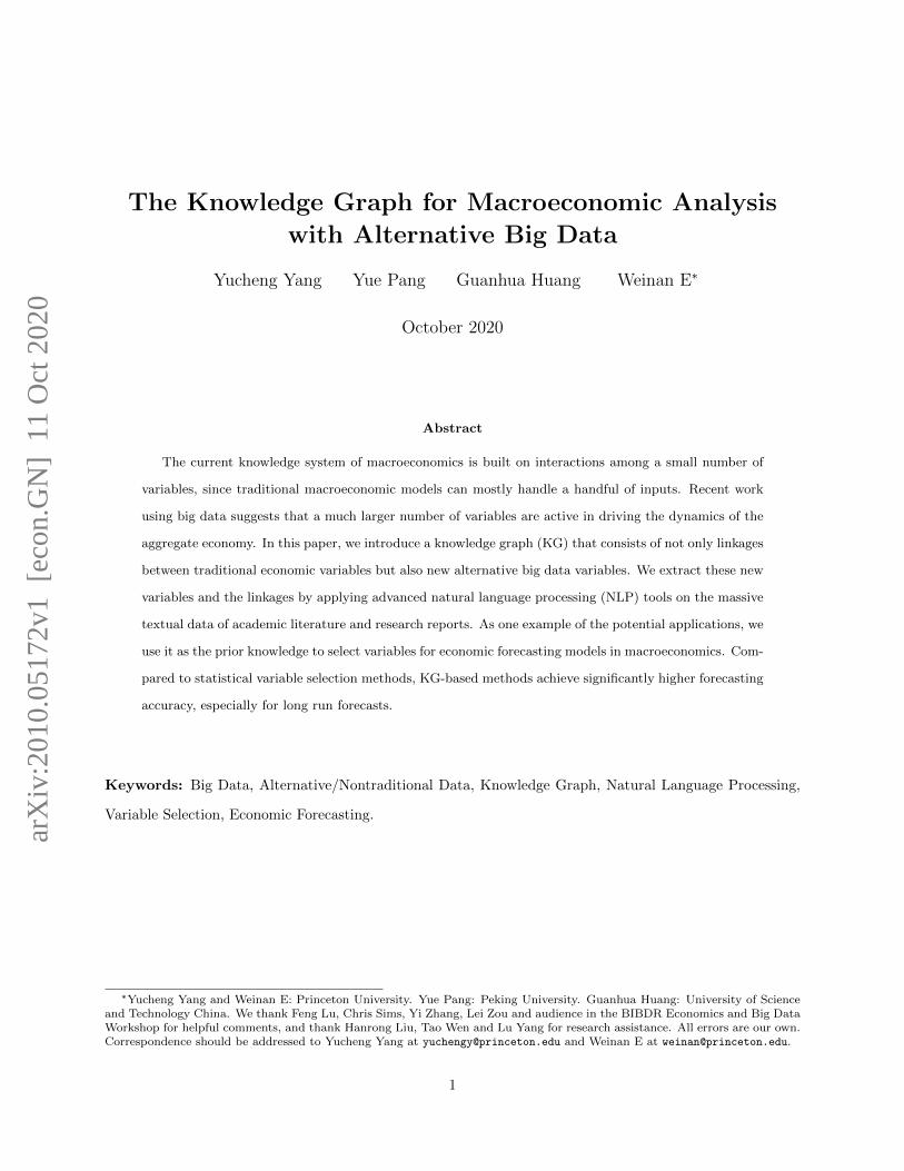
1 Introduction
Traditional macroeconomic models, whether statistical models like VAR (Sims, 1972) or structural models
like DSGE (Christiano, Eichenbaum, and Evans, 2005; Smets and Wouters, 2007), can only handle a handful
of variables. At the same time, the whole knowledge system of macroeconomics is built on our understanding
of the interactions among these small number of variables. With the rise of big data and machine learning,
we now have the opportunity to develop more sophisticated models with a much larger number of variables
(McCracken and Ng, 2016; Coulombe et al., 2019). In order to do this effectively, a new knowledge system
is needed to describe both the statistical and structural relationships of the traditional as well as the many
new economic variables.
(a) Knowledge Graph used by Google Search Engine
decrease
increase
increase
Inflation Rate
Moneysupply
...
SeasonalEffect
Crude oilimport
Urbanwage
...baselinedepositinterest
rate
relate
relate
urbanmigrationworker
shortageCrude oil
internationalprice decrease
relate
relate
agriculturelabor
demand
Crop price
increase
increase
increase
increase
...
relate
increasefood price
(b) Knowledge Graph of Economic Variables
Figure 1: Examples of Knowledge Graphs
In this paper, we discuss how to build such a knowledge graph (KG)1 of the linkages between traditional
economic variables and alternative data variables. We use advanced natural language processing (NLP) tools
to extract such alternative data variables and their linkages from massive dataset the consists of academic
1Knowledge graph (KG) is a commonly used knowledge base structure that use graph topology to represent interlinkeddescriptions of entities. It has been widely used in many real world knowledge system applications like Google search engine(Singhal, 2012), Wikipedia encyclopedia, Facebook social networks, Apple’s Siri, among many others. An example of knowledgegraph used in Google search is illustrated in the left panel of Figure 1. In Google’s KG, it links many entities to famous peopleand store their relationships, like June 1723 as Adam Smith’s birth month, and Kirkcaldy as his birth place. Such kind of{subject, predicate, object} triple structure like {Adam Smith, birth place, Kirkcaldy} is called RDF (Resource DescriptionFramework) triples in the terminology of knowledge graph. When a user search for Adam Smith’s birth place, Google wouldprovide webpages relevant to the entity “Kirkcaldy” based on this knowledge graph, even though those webpages may not bedirect results of Google search algorithms like PageRank.
2

literature and research reports. Specifically, we design an algorithm to extract from massive textual data (1)
traditional variables of interest (like GDP, inflation rate, housing price, etc.), (2) alternative data variables
(like electricity usage, migration flow, etc.), as well as (3) the relationships (positive correlation, negative cor-
relation, etc.) among these variables. After some post-processing including resolving coreferences, we build a
knowledge graph by starting with traditional variable of interests as the centers, and expanding in a step-wise
fashion to include the relevant alternative variables. A very small subgraph of the resulted knowledge graph
centered at inflation rate is illustrated in the right panel of Figure 1. This graph displays the conceptional
relationship between inflation rate and other concepts discussed in the massive textual data we study in this
paper. Some of these linkages have already been well studied in the literature, for example money supply will
increase the inflation rate; the increase of benchmark interest rate may decrease the inflation rate. But there
are also linkages that carry new information. For example, we learn from some of these research reports that
the increase of urban migration worker shortage may affect inflation, through the increase of urban wages
(upper right corner of Figure 1).
The knowledge graph we construct provides a new knowledge system for macroeconomics, and has many
potential applications. One application we are particularly interested in is to formulate macroeconomics as
a problem of reinforcement learning (RL) (Sutton and Barto, 2018; Silver et al., 2016). A RL framework
consists of the following essential components: the state space and the environment, the action space, the
system dynamics and the reward functions. In this regard, the knowledge graph of linkages among economic
variables plays the role of the state space and the environment. In a companion paper (Yang, Shao, and E,
2020), we construct a structured framework of economic policy targets and policy tools. The framework for
the policy tools plays the role of the action space in the RL framework, whereas the framework for the policy
targets acts as the reward functions. In this paper, we also apply the knowledge graph of economic variables
to a simple but more concrete task: variable selection in economic forecasting. Different from previous work
using statistical tools to do variable selection, we use the knowledge graph as the prior knowledge to select
variables for economic forecasting models. We will see that compared to statistical methods, the KG-based
method achieves significantly higher forecasting accuracy, especially for long term forecasts.
This paper contributes to the following literature. First, we contribute to the literature on using big data and
machine learning tools in macroeconomics (McCracken and Ng, 2016; Stock and Watson, 2016; Giannone
et al., 2008; Coulombe et al., 2019; Fan et al., 2020a). Most of previous work apply or modify off-the-shelf ma-
3

chine learning tools to study high dimensional macroeconomic variables, while we stand out to design a new
knowledge system for macroeconomics with big data. Second, we contribute to the literature on knowledge
graph and knowledge extraction in science. Besides prominent applications in industry, knowledge graph
has also been used for knowledge extraction and knowledge representation in various scientific disciplines
(Luan et al., 2018), for example material science and physics. Last but not the least, our application example
contributes to the literature on variable selection and model reduction in economic forecasting with big data.
Previous methods rely on statistical learning, including shrinkage methods like Lasso (Tibshirani, 1996),
Bayesian methods (Sims and Zha, 1998; Doan, Litterman, and Sims, 1984) and machine learning methods
like factor models (Fan, Li, and Liao, 2020b) and autoencoder (Goodfellow, Bengio, and Courville, 2016).
Our work provides a new method for variable selection, through a systematic treatment of existing human
knowledge.
The remaining of the paper is organized as follows. In Section 2, we introduce the textual data that we
use to construct the knowledge graph, as well as the data we use in our application example. In Section
3, we present the detailed algorithm for constructing the knowledge graph from massive textual data. We
discuss the application of the knowledge graph on forecasting in Section 4. In particular, we use it as the
prior knowledge to do variable selection for economic forecasting. Finally we conclude with discussions on
the future work.
2 Data
2.1 Textual Data for Knowledge Graph Construction
We build the knowledge graph (KG) of linkages among economic variables by extracting variables and their
relationships from the massive dataset that consists of previous research documents. In general, two different
types of textual data are suited for our work: academic papers published by leading journals in economics, or
research reports published by leading think tanks, consulting firms, asset management companies and other
similar agencies (“industry research reports” hereafter). In this paper, we use Chinese industry research
reports as the major textual data source. We make this choice for the following reasons. First, most of
those industry research reports focus on analyzing or forecasting the dynamics of aggregate variables, and
it is always clearly stated what variables are studied in each report. Second, these reports mostly adopt
the narrative approach (Shiller, 2017) in research, which clearly state the logic chains of their analysis in
4
narrative language, rather than in theoretical or quantitative models which is more common in English papers
or industry reports. Thirdly, they are freely available and can be downloaded from the WIND database2. We
download3 all the industry research reports from the macroeconomic research section of the WIND database,
and selected 846 of them that adopt the narrative approach to study certain variables of interest as the
textual data for this paper.
2.2 Traditional and Alternative Data for Economic Forecasting
As an application of the knowledge graph we construct, we use it as the prior knowledge to select variables for
economic forecasting models. In Section 4.2, we forecast China’s monthly inflation and nominal investment
time series using both traditional variable selection method and the KG-based method. For the traditional
method, the input variables come from the standard Chinese monthly time series constructed by Higgins and
Zha (2015) and Higgins, Zha, and Zhong (2016)4. For the period of 1996 to 2019, there are 12 monthly time
series available: Real GDP, Nominal Investment, Nominal Consumption, M2, Nominal Imports, Nominal Ex-
ports, 7-Day Repo, Benchmark 1-year Deposit Rate, Nominal GDP, GDP Deflator, CPI and Investment Price.
For the KG-based method, we design model inputs under the guidance of the knowledge graph, and obtain
as many data variables as we can from two major databases on Chinese economy: WIND and CEIC. The
full list of alternative indicators we obtain are discussed in Section 4.2.
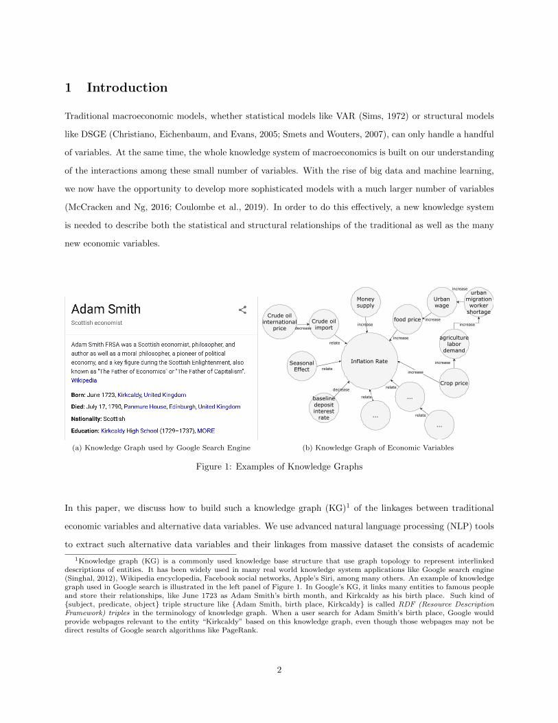
3 Construction of Knowledge Graph
3.1 An Example: From Textual Data to Knowledge Graph
Before presenting the detailed algorithm for extracting variables and their relations from the textual data,
we illustrate the main idea with an example. The following paragraph is translated from a research report5
from a leading think tank in China. It studies the dynamics of inflation rate using alternative data variables.
We will explain how to build part of the knowledge graph from this paragraph step by step.
2The WIND database is often referred to as the Chinese version of Bloomberg terminal, and is the major provider ofmacroeconomic and financial data and information in China. WIND also provides millions of industry research reports on themacroeconomy, industries or even individual public firms for download, which is not available on Bloomberg terminals.
3We downloaded all reports available on August 9, 2018 when we started this project.4The data is available at https://www.frbatlanta.org/cqer/research/china-macroeconomy, last accessed on August 21,
2020.5The full text of this report (in Chinese) is available https://www.nsd.pku.edu.cn/jzky/ceojjgcbgk/252274.htm., last
accessed on August 15, 2020.
5
“Dr. Gao concluded that a long-term systematic migrant worker shortage began to appear in the Chinese
migrant labor market around 2005, which greatly increased the growth rate of migrant workers’ wages,
resulted in the increase of food prices, and pushed up the increase in consumer price index, making the
average level of inflation probably 100 to 200 basis points higher.”
In this example, we hope to extract all the economic variables6 and the relation keywords among those
variables, store them in RDF (Resource Description Framework) triples of {variable 1, relation, variable 2}
format, and construct the knowledge graph from the RDF triples.
As the first step, we find the traditional variables of interest in this paragraph: consumer price index and
inflation. These variables are the center nodes of the knowledge graphs. Next, we find the alternative vari-
ables that are measurable with economic data: food prices, migrant workers’ wages, migrant worker shortage.
Thirdly, we find the key words linking these variables and the inflation variable: making...higher, push up,
resulted in, increase. The extraction of all the economic variables and the relation keywords among
those variables are highlighted in the box below.
“Dr. Gao concluded that a long-term systematic migrant worker shortage began to ap-
pear in the Chinese migrant labor market around 2005, which greatly increased the
growth rate of migrant workers’ wages, resulted in the increase of food prices, and pushed
up the increase in consumer price index, making the average level of inflation probably 100 to 200
basis points higher .”
We store all the results of the extraction process in RDF triples of {variable 1, relation, variable 2} format:
• {migrant worker shortage, increase, growth rate of migrant workers’ wages}
• {growth rate of migrant workers’ wages, resulted in the increase, food prices}
• {food prices, push up, consumer price index}
• {food prices, make higher, inflation}
Later we will classify all the relation keywords into three classes: “increase”, “decrease”, “neutral”. All the
relation keywords here belong to the “increase” class. The last two RDF triples are equivalent to each other,
6An economic variable is an object measurable with economic data. It could be traditional variables like GDP, inflation, andcould also be alternative variables like migration flow, oil prices, among others.
6

so the duplicates will be dropped when constructing the knowledge graph. This process gives rise to the
subgraph in the upper right corner of Figure 2.
decrease
increase
increase
Inflation Rate
...
...
...
...
Urbanwage
...
...
relate
relate
urbanmigrationworker
shortage
...decrease
relate
relate
...
...
increase
increase
increase
increase
...
relate
increasefood price
Figure 2: Knowledge Graph of Economic Variables: A Subgraph around the Inflation Rate
3.2 Construction Procedure
Inspired by the example above, now we present the general procedures of constructing the knowledge graph
of linkages among economic variables from the textual data.
Step 1. Make a list of aggregate variables of interest, together with their variants.
For this paper, we investigate the following variables (with their variants in the brackets): GDP (output,
economic growth), Investment, Housing price (housing market, real estate market, real estate price),
RMB Exchange Rate (RMB), Inflation (CPI).
Step 2. Find all these aggregate variables and their variants in the documents with string matching.
Step 3. For each aggregate variable detected in the documents, find all the other variables around it, as well as
the relation among aggregate variables and other variables.
Step 4. Represent all the variables and relations that have been extracted with the typical RDF triple structure
in a knowledge graph.
7
Step 5. Merge all the co-references and build the knowledge graph.
Among all the procedures above, Steps 1, 2 and 4 are straightforward to implement, while Steps 3 and 5 are
technically more challenging. We will discuss the challenges and how we address them in the next subsection.
3.3 Main Challenges of Knowledge Graph Construction and Solutions
The most challenging steps of constructing the knowledge graph are the extraction of variable entities and
relations, as well as co-reference resolution.
Economic variables, especially alternative variables, exhibit complicated semantic patterns that have not
been investigated in classical entity recognition and co-reference resolution tasks (Ji et al., 2020; Hogan
et al., 2020). Typically, entity recognition tasks include two steps: (1) identify regions of text that may cor-
respond to entities, (2) categorize them into a predefined list of types (people, organization, location, among
many others) (Ling and Weld, 2012). Most of the literature take outputs from the first step as given, and
focus on improving the classification work in the second step. However, in our problem, the first step is crucial
and nontrivial, since economic variables are mostly multi-token entities with complicated semantic patterns.
Examples of complicated variable entities include “migration worker shortage”, “growth rate of migration
workers’ wages”, “processing firm registrations in China”, “leverage rate of local government financing ve-
hicles”. As a result, it is challenging to identify boundaries of the text that mentions a variable entity. For
the second step, previous work mostly focuses on categorizing entities into names of people, organizations,
locations, or other more detailed types labeles in large knowledge database like Freebase (Ling and Weld,
2012; Hogan et al., 2020), and are not suitable for classifying variable entities in our paper. Similarly, due to
the complicated semantic patterns of economic variables, co-reference resolution, or entity disambiguation,
is particularly challenging in our setting.
To address these challenges, we design a recursive weakly supervised learning algorithm (Zhou, 2018) with
some human involvement7 to extract variable entities and entity relations from the textual data. In each
iteration, we first identify regions of text that are most likely to have variable entities or relations, and
then use human editor to select true variable entities or relations, and take the improved set into the next
iteration. Our algorithm is similar to but different from the bootstrapping approach of entity recognition
7To note, it is a common practice to involve direct contributions from human editors to construct knowledge graphs. Someprominent knowledge graphs are primarily constructed with human efforts (Hogan et al., 2020).
8
(Collins and Singer, 1999; Gupta and Manning, 2014). To make this facilitation scheme work, we reduce the
general notion of relation extraction to extracting only the “relation keywords” in the textual data. In terms
of co-reference resolution, we also combine a similarity score measure and some human efforts to remove
duplicates of entities.
3.3.1 Entity Recognition: Variable Names and Relation Keywords
The weakly supervised learning algorithm to extract variable entities and relation keywords from the textual
data works as follows:
Step 1. Construct an initial set of economic variables and an initial set of relation keywords. The initial set of
economic variables are from the macroeconomic database of WIND. The initial set of relation keywords
are commonly seen relation words and phrases like increase, decrease, result in, push up, among others.
Step 2. Using the current set of economic variables as training data, train a simple model to predict whether a
phrase8 is a variable. With the model we can get a confidence metric for each phrase to be a variable.
Human editors select true variables from those high-confident phrases to get an expanded variable set.
Step 3. Find sentences that contain many variables, but very few relation keywords. Then use the human
editors to find the relation keywords in these sentences. Expand the set of relation keywords.
Step 4. Find sentences that contain relation keywords, but very few variables. Then use the human editors to
find the variables in those sentences. Repeat Step 2 to expand the variable set.
Step 5. Repeat Steps 3 and 4, until we cannot find any new relation keywords or variables.
3.3.2 Co-reference Resolution
We define the similarity score between two economic variable entities represented as two word vectors:
Sim(u, v) = 1− u · v‖u‖2‖v‖2
where u, v are word vectors of the two variables. Based on this score, we get those economic variable entities
with high similarity scores with each other. Human editors will determine the true duplicates from those
high similarity pairs. Then we unify the names of those variable entities that are co-references with each
other. The unification process is done by human editors to choose the best entity name that would show up
8A phrase is a N-gram object after word segmentation, where N could be small integers with N ≤ 5.
9
in the knowledge graph. After the name unification, we remove the duplicated RDF triples, and build the
final knowledge graph based on the unique RDF triples we get.
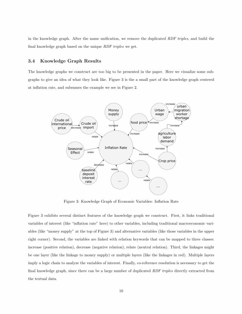
3.4 Knowledge Graph Results
The knowledge graphs we construct are too big to be presented in the paper. Here we visualize some sub-
graphs to give an idea of what they look like. Figure 3 is the a small part of the knowledge graph centered
at inflation rate, and subsumes the example we see in Figure 2.
decrease
increase
increase
Inflation Rate
Moneysupply
...
SeasonalEffect
Crude oilimport
Urbanwage
...baselinedepositinterest
rate
relate
relate
urbanmigrationworker
shortageCrude oil
internationalprice decrease
relate
relate
agriculturelabor
demand
Crop price
increase
increase
increase
increase
...
relate
increasefood price
Figure 3: Knowledge Graph of Economic Variables: Inflation Rate
Figure 3 exhibits several distinct features of the knowledge graph we construct. First, it links traditional
variables of interest (like “inflation rate” here) to other variables, including traditional macroeconomic vari-
ables (like “money supply” at the top of Figure 3) and alternative variables (like those variables in the upper
right corner). Second, the variables are linked with relation keywords that can be mapped to three classes:
increase (positive relation), decrease (negative relation), relate (neutral relation). Third, the linkages might
be one layer (like the linkage to money supply) or multiple layers (like the linkages in red). Multiple layers
imply a logic chain to analyze the variables of interest. Finally, co-reference resolution is necessary to get the
final knowledge graph, since there can be a large number of duplicated RDF triples directly extracted from
the textual data.
10
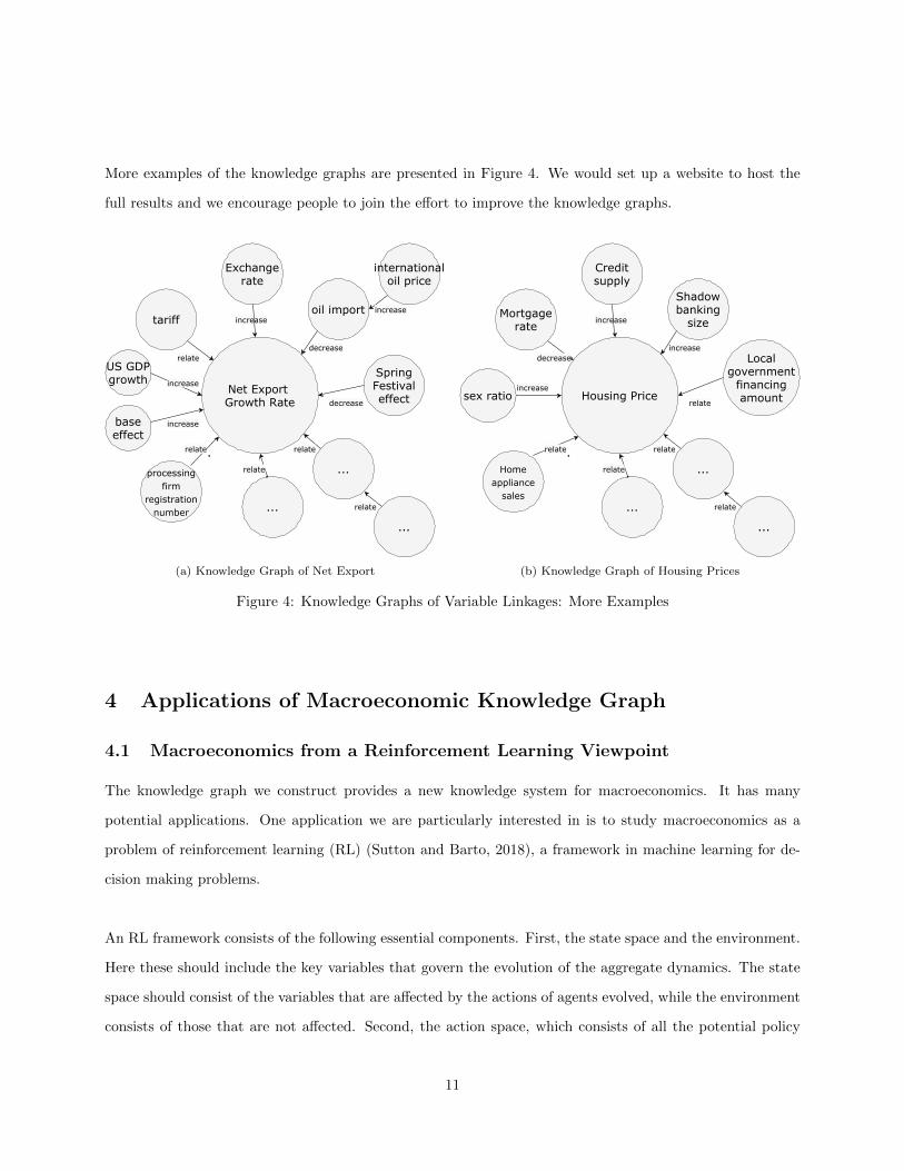
More examples of the knowledge graphs are presented in Figure 4. We would set up a website to host the
full results and we encourage people to join the effort to improve the knowledge graphs.
increase
decrease
increase
Net Export Growth Rate
Exchangerate
...
US GDPgrowth
tariff
internationaloil price
...
baseeffect
increase
relate
relate
relate
SpringFestivaleffectdecrease
...
relate
increaseoil import
processingfirm
registrationnumber
relate
(a) Knowledge Graph of Net Export
increase
increase
Housing Price
Creditsupply
...
sex ratio
Mortgagerate
...
increase
decrease
relate
relate
Localgovernment
financingamountrelate
...
relate
Shadowbanking
size
Homeappliance
sales
relate
(b) Knowledge Graph of Housing Prices
Figure 4: Knowledge Graphs of Variable Linkages: More Examples
4 Applications of Macroeconomic Knowledge Graph
4.1 Macroeconomics from a Reinforcement Learning Viewpoint
The knowledge graph we construct provides a new knowledge system for macroeconomics. It has many
potential applications. One application we are particularly interested in is to study macroeconomics as a
problem of reinforcement learning (RL) (Sutton and Barto, 2018), a framework in machine learning for de-
cision making problems.
An RL framework consists of the following essential components. First, the state space and the environment.
Here these should include the key variables that govern the evolution of the aggregate dynamics. The state
space should consist of the variables that are affected by the actions of agents evolved, while the environment
consists of those that are not affected. Second, the action space, which consists of all the potential policy
11
functions taken by agents (including households, firms and government agencies) in the economy. Third, the
system dynamics, the evolution law of the aggregate economy. This can either be model-based in which case
we use a postulated dynamic model for the aggregate economy, or model-free in which case we rely purely
on observational data. Fourth, the reward functions, here the utility functions of agents involved. In this
regard, the knowledge graph of linkages among economic variables helps to define the state space and the
environment of the economy. In a companion paper (Yang, Shao, and E, 2020), we construct a structured
framework of economic policy tools and policy targets. The structure for the policy tools plays the role of
the action space in the RL framework, whereas the policy targets act as the reward functions of government
agencies. Such a framework could potentially allow us to make maximum use of existing knowledge and data
to study the macroeconomy.
4.2 Example of Application: Knowledge Graph for Economic Forecasting
As a more concrete example, we apply the knowledge graph to the problem of variable selection in economic
forecasting. Different from previous work using statistical tools to do variable selection (Tibshirani, 1996;
Zou and Hastie, 2005; Sims and Zha, 1998; Goodfellow et al., 2016; Fan et al., 2020a), we combine statistical
tools with the knowledge graph as the prior knowledge to select variables for economic forecasting models.
Hopefully this will provide a new method for variable selection that uses systematically all existing human
knowledge.
Here the task is to forecast China’s monthly inflation rate and nominal investment time series from April
1996 to June 20199. For each i = 1, 2, ..., 12, we hope to build a model to forecast the inflation rate or
nominal investment yt+i in i months ahead, with input variables from the past three months {Xs}ts=t−3:
yt+i = f({Xs}ts=t−3)
In traditional statistical method, economists have little idea of what variables should be used as model inputs
and what should not, so they typically find a standard dataset as input, and use statistical variable selection
methods to estimate the model. In this spirit, we use the 12 time series variables10 from the standard Chinese
monthly time series constructed by Higgins and Zha (2015) and Higgins, Zha, and Zhong (2016), and use
9The time range is chosen to have as many data observations as possible while still having a reasonably large number ofinput variables for both methods.
10They are Real GDP, Nominal Investment, Nominal Consumption, M2, Nominal Imports, Nominal Exports, 7-Day Repo,Benchmark 1-year Deposit Rate, Nominal GDP, GDP Deflator, CPI and Investment Price.
12
Lasso (Tibshirani, 1996) as the variable selection method.
For the KG-based method, we design model inputs with the guidance of the knowledge graph results in
Section 3.4, and obtain as many alternative data variables as we can from WIND and CEIC. Among all the
alternative data variables11 that are directly linked to inflation rate in the knowledge graph, the following
variables are available in the full model sample period (October 1996 to June 2019): CPI (historical data),
GDP, benchmark 1-year deposit interest rate, benchmark 1-year loan interest rate, nationwide fiscal expendi-
ture, urbanization rate, central government fiscal expenditure, share of manufacturing output in GDP, urban
unemployment rate, worldwide GDP growth rate, M1 money supply, M2 money supply, USD/RMB exchange
rate, crude oil production, raw coal production, copper production, raw coal production, Non-ferrous metal
production, OPEC Basket Price, crude oil import amount, raw coal import amount, copper import amount,
steel import amount, Spring Festival dummy, National Day Festival dummy. Among all the alternative data
variables that are directly linked to nominal investment in the knowledge graph, the following variables are
available in the full model sample period (April 1996 to June 2019): nominal investment (historical data),
GDP, benchmark 1-year deposit interest rate, benchmark 1-year loan interest rate, nationwide fiscal ex-
penditure, central government fiscal expenditure, refinery capacity, metal smelter capacity, economic policy
uncertainty (EPU) index, tariff income, tax income, stock market return, stock market volatility, dummy
variable for the reform of replacing business tax with value-added tax, dummy variable for central leadership
transition, M1 money supply, M2 money supply, Spring Festival dummy, National Day Festival dummy.
These variables are used in Lasso regression to give the KG-based model prediction.
For different forecasting periods (from one month to 12 months), the forecasting errors on the test sets for
both the baseline model and KG-based model are presented in Figure 5. We report the mean absolute per-
centage error (MAPE) in the left panels, and the root mean squared error (RMSE) in the right panels, and the
results are qualitatively the same. For inflation forecasting (upper panels), compared to the baseline model,
the KG-based model achieves higher forecasting accuracy in general. In short term forecasting (within five
months), the forecasting errors for both models are comparable to each other, and the baseline model even
outperforms the KG-based model in some horizons. However, in long run forecasting, the performance of the
baseline model gets worse, while the KG-based model achieves a stable and much higher accuracy than the
baseline method. Similar arguments also hold for nominal investment forecasting (bottom panels in Figure 5).
11We convert all variables into the monthly frequency.
13

� � � �� ��
������������������������
�����
�����
�����
�����
�����
�����
�����
��
�
��������������������������������������
(a) MAPE of Inflation Forecasting
� � � �� ��
������ ����������������
����
����
����
����
����
��
��
������������ ������������������ ������
(b) RMSE of Inflation Forecasting
� � � � �� ��
�������������������������
����
����
����
����
����
����
���
����������������� �����������������
(c) MAPE of Investment Forecasting
� � � �� ��
������ �������������
���
���
���
���
���
���
���
��
��
������������ ������������������ ������
(d) RMSE of Investment Forecasting
Figure 5: Forecasting Errors of Baseline Model vs. KG-Based Model
The general trend revealed by Figure 5 are consistent with our expectation that short term forecasting relies
more on data, while long term forecasting relies more on capturing the underlying logic in the problem.
The baseline model is more of a pure data-driven model, whereas the KG-based model tries to capture the
underlying logic. The better long term performance of the KG-based model serves as a confirmation that
the relationships described in the knowledge graph correctly represents the true logic of the economic system
under investigation.
Periods ahead 1 2 3 4 5 6 7 8 9 10 11 12P-value: inflation 0.1102 0.0157 0.0248 0.0971 0.3213 0.0000 0.0002 0.0099 0.0020 0.0002 0.0000 0.0002
P-value: investment 0.1128 0.0799 0.5677 0.0941 0.0162 0.0406 0.0005 0.2295 0.0426 0.0064 0.0104 0.0693
Table 1: The p-values of Diebold-Mariano Tests
To check the significance of these comparisons, we perform the Diebold-Mariano (DM) test (Diebold and
14
Mariano, 1995; Harvey, Leybourne, and Newbold, 1997) for both forecasting problems. We report the p-
values of the DM tests for different forecasting periods ahead in Table 1. Most of the comparison results are
significant, which again confirms our findings.
5 Conclusion
In the age of big data, traditional knowledge system of macroeconomics that built on interactions among a
small number of variables is faced with severe challenges. In this paper, we develop an approach to build
a knowledge graph (KG) of the linkages between traditional economic variables and massive alternative big
data variables. We extract these variables and linkages by applying advanced natural language processing
(NLP) tools on the massive dataset that consists of academic literature and research reports.
The knowledge graph we construct has many potential applications. In this paper, we use it as the prior
knowledge to select variables for economic forecasting models in macroeconomics. Compared to statistical
variable selection methods, KG-based method achieves lower forecasting errors, especially for long run fore-
casts. In this particular example, we only make use of the list of variables around the variable of interest (like
inflation) in the knowledge graph, rather than the multi-layer graphical structure of knowledge embedding.
Future research can further investigate how to incorporate this structure into the statistical model, possibly
in the form of model structure restrictions. Future work may also investigate other potential applications of
this new knowledge system, like the reinforcement learning framework of macroeconomics we discuss briefly
in this paper.
References
Christiano, Lawrence J, Martin Eichenbaum, and Charles L Evans (2005), “Nominal rigidities and the dy-namic effects of a shock to monetary policy.” Journal of Political Economy, 113, 1–45.
Collins, Michael and Yoram Singer (1999), “Unsupervised models for named entity classification.” In 1999Joint SIGDAT Conference on Empirical Methods in Natural Language Processing and Very Large Corpora.
Coulombe, Philippe Goulet, Maxime Leroux, Dalibor Stevanovic, and Stephane Surprenant (2019), “How ismachine learning useful for macroeconomic forecasting?” Technical report, CIRANO.
Diebold, Francis X and Robert S Mariano (1995), “Comparing predictive accuracy.” Journal of Business &economic statistics, 20, 134–144.
Doan, Thomas, Robert Litterman, and Christopher Sims (1984), “Forecasting and conditional projectionusing realistic prior distributions.” Econometric reviews, 3, 1–100.
15

Fan, Jianqing, Yuan Ke, and Kaizheng Wang (2020a), “Factor-adjusted regularized model selection.” Journalof Econometrics.
Fan, Jianqing, Kunpeng Li, and Yuan Liao (2020b), “Recent developments on factor models and its applica-tions in econometric learning.” arXiv preprint arXiv:2009.10103.
Giannone, Domenico, Lucrezia Reichlin, and David Small (2008), “Nowcasting: The real-time informationalcontent of macroeconomic data.” Journal of Monetary Economics, 55, 665–676.
Goodfellow, Ian, Yoshua Bengio, and Aaron Courville (2016), Deep learning. MIT press.
Gupta, Sonal and Christopher D Manning (2014), “Improved pattern learning for bootstrapped entity extrac-tion.” In Proceedings of the Eighteenth Conference on Computational Natural Language Learning, 98–108.
Harvey, David, Stephen Leybourne, and Paul Newbold (1997), “Testing the equality of prediction meansquared errors.” International Journal of forecasting, 13, 281–291.
Higgins, Patrick, Tao Zha, and Wenna Zhong (2016), “Forecasting China’s economic growth and inflation.”China Economic Review, 41, 46–61.
Higgins, Patrick C and Tao Zha (2015), “China’s macroeconomic time series: Methods and implications.”Unpublished Manuscript, Federal Reserve Bank of Atlanta.
Hogan, Aidan, Eva Blomqvist, Michael Cochez, Claudia d’Amato, Gerard de Melo, Claudio Gutierrez, JoseEmilio Labra Gayo, Sabrina Kirrane, Sebastian Neumaier, Axel Polleres, et al. (2020), “Knowledge graphs.”arXiv preprint arXiv:2003.02320.
Ji, Shaoxiong, Shirui Pan, Erik Cambria, Pekka Marttinen, and Philip S Yu (2020), “A survey on knowledgegraphs: Representation, acquisition and applications.” arXiv preprint arXiv:2002.00388.
Ling, Xiao and Daniel S Weld (2012), “Fine-grained entity recognition.” In Proceedings of the Twenty-SixthAAAI Conference on Artificial Intelligence, 94–100.
Luan, Yi, Luheng He, Mari Ostendorf, and Hannaneh Hajishirzi (2018), “Multi-task identification of en-tities, relations, and coreference for scientific knowledge graph construction.” In Proceedings of the 2018Conference on Empirical Methods in Natural Language Processing (EMNLP), 3219–3232.
McCracken, Michael W and Serena Ng (2016), “FRED-MD: A monthly database for macroeconomic re-search.” Journal of Business & Economic Statistics, 34, 574–589.
Shiller, Robert J (2017), “Narrative economics.” American Economic Review, 107, 967–1004.
Silver, David, Aja Huang, Chris J Maddison, Arthur Guez, Laurent Sifre, George Van Den Driessche, JulianSchrittwieser, Ioannis Antonoglou, Veda Panneershelvam, Marc Lanctot, et al. (2016), “Mastering thegame of go with deep neural networks and tree search.” Nature, 529, 484–489.
Sims, Christopher A (1972), “Money, income, and causality.” The American Economic Review, 62, 540–552.
Sims, Christopher A and Tao Zha (1998), “Bayesian methods for dynamic multivariate models.” InternationalEconomic Review, 949–968.
Singhal, Amit (2012), “Introducing the knowledge graph: things, not strings.” Google Blog, URL https:
//www.blog.google/products/search/introducing-knowledge-graph-things-not/.
Smets, Frank and Rafael Wouters (2007), “Shocks and frictions in us business cycles: A bayesian dsgeapproach.” American Economic Review, 97, 586–606.
16
Stock, James H and Mark W Watson (2016), “Dynamic factor models, factor-augmented vector autoregres-sions, and structural vector autoregressions in macroeconomics.” In Handbook of macroeconomics, volume 2,415–525, Elsevier.
Sutton, Richard S and Andrew G Barto (2018), Reinforcement learning: An introduction. MIT press.
Tibshirani, Robert (1996), “Regression shrinkage and selection via the lasso.” Journal of the Royal StatisticalSociety: Series B (Methodological), 58, 267–288.
Yang, Yucheng, Zihao Shao, and Weinan E (2020), “Understanding China’s policy making via machinelearning.” Technical report, Princeton University.
Zhou, Zhi-Hua (2018), “A brief introduction to weakly supervised learning.” National Science Review, 5,44–53.
Zou, Hui and Trevor Hastie (2005), “Regularization and variable selection via the elastic net.” Journal of theroyal statistical society: series B (statistical methodology), 67, 301–320.
17