Embed Size (px)
Citation preview

THE J = 0 - 1 ROTATIONAL TRANSITIONS
OF THE PARTIALLY DEUTERATED
METHYL ALCOHOLS
by
HOWARD RAEBURN TEST II, B.A.
A THESIS
IN
PHYSICS
Submitted to the Graduate Faculty of Texas Technological College
in Partial Fulfillment of the Requirements for
the Degree of
MASTER OF SCIENCE
Approved
Accepted
August, 1968

1^3 ' •'? ^'
Cop. ^
ACKNOWLEDGEMENT
I would like to express my appreciation to Dr. C. R. Quade for his
guidance and helpful criticism in the direction of this thesis, to my
wife, Pamela, for her help with the initial draft, and to Mrs. Charlotte
Hutcheson for her most proficient typing.
ii

TABLE OF CONTENTS
Page
ACKNOWLEDGEMENT ii
LIST OF TABLES iv
LIST OF FIGURES v
CHAPTER
I. INTRODUCTION 1
II. THEORETICAL BACKGROUND 4
Rigid Rotor 4
Simplified Calculation Including Effects from
Internal Rotation 9
Stark Effect " 16
Line Shape and Intensity 19
III. THE SPECTROGRAPH 23
IV. EXPERIMENTAL TECHNIQUE " 45
V. ANALYSIS OF DATA . . . 50
LIST OF REFERENCES 64
APPENDIX I 66
APPENDIX II 69
APPENDIX III 70
111

LIST OF TABLES
Table Page
1. Rigid Rotor Rotational Constants for
CH OH, CH^DOH, and CHD2OH 10
2. Averaged Rotational Constants for CH DOH and CHD_OH . . . . 13
3. The Klystrons Used in This Work 23
4. Stark Measurements of CH OH, CH DOH, and CHD^OH 51
5. The J = 0 - 1 Transitions in CH OH, CH DOH, and
CHD2OH 7 59
6. Calibration of the Squarewave Generator 50
7. Relative Intensities of the J = 0 - 1 Transitions
in CH DOH and CHD^OH 61 8. Calculated Relative Intensities of the J = 0 1
Transitions in CH DOH and CHD OH . 62
IV

LIST OF FIGURES
Figure ^ Page
1. Equilibrium Orientation of Methyl Alcohol . . . . 2
2. The Spectrograph 24
3. Oscilloscope Display of a Spectral Line 26
4. Frequency Drive 27
5. Chart Display of a Spectral Line 28
6. Klystron Power Supply 30
7. Detail of the Absorption Cell 32
8. Low-Noise Preamplifier 35
9. Lock-In Amplifier 36
10. Squarewave Generator 40
11. Frequency Measurement System 41
12. Standard Frequency Mixer 43
13. Diode Mixer Mount 43
14. Analysis of Chart Display 48
15. Structure of Methyl Alcohol 67
CHAPTER I
INTRODUCTION
Some low pressure gases selectively absorb electromagnetic radiation
of particular wavelengths in the millimeter and centimeter region. The
study of this phenomenon is known as microwave spectroscopy of gases.
The wavelengths or.frequencies at which absorptions occur are inter-
pretable in terms of the structure and behavior of the absorbing
molecule. The motions of electrons in atoms and molecules are known t'o
produce spectra in the optical and ultraviolet region while the slower
vibrational motions of atoms in molecules are primarily responsible for
the infrared spectra. It is the still slower overall rotations of mole
cules which have frequencies that lie in the microwave region.
Information that can be learned from rotational spectra includes
structures of relatively simple molecules, molecular electric dipole
moments, polarizabilities of molecules by electric fields, and potential
1* barriers hindering internal motions.
Methyl alcohol is one of the lightest and simplest molecules which
is capable of internal rotation. In this molecule (Figure 1) the 0-H
group rotates about the CH symmetry axis. Until recently investigation
of the microwave spectra of methyl alcohol has been limited to those iso-
9 A
topic species with symmetric internal rotors due to a lack of a
suitable theoretical model to describe the motion of the asymmetric
internal rotor. In 1963 a suitable model was developed, which is based
on one degree of internal freedom, from which the torsional and rotational
'**The superscript numbers refer to the List of Ro,ferences.
1

ri^aiLc^iti-iiir :L'^SZ
H
H
H H
Eclipsed Configurat ion
(a = IT)
H
Staggered Configuration
(a = 0)
Figure 1 Equilibrium Orientation
of Methyl Alcohol

energies may be calculated. The theory has been applied to calculations
for CH DOH and the results indicate that the fine structure of the
J = 0 -> 1 transition should depend upon the equilibrium orientation of
o
the methyl and hydroxyl groups.
This thesis reports the investigation of the J = 0 -> 1 rotational
transitions of CH DOH and CHD^OH. A rigid rotor calculation showed that
these transitions should occur around 44650 MHz for CH DOH and 41634 MHz
for CHD»0H. Absorption lines have been found, identified, and assigned
by the Stark effect and finally assigned to torsional states by relative
intensity measurements.
Nine absorption lines for each isotopic species have been identified
as originating from the J = 0 1 transition. Three lines have been
assigned to the torsional ground state which indicates the rotational
motion is perturbed by hindered internal rotation. Two lines have been
assigned to each of the next three torsional states. The assignment sug
gests that the internal rotation is nearly free in excited torsional
states.
To determine the equilibrium orientation of methyl alcohol, only the
frequencies of the n = 0 lines and their differences in frequency should
be needed. The results of this analysis, which admittedly are crude,
suggest the staggered configuration to be of lower energy.

CHAPTER II
THEORETICAL BACKGROUND
Rigid Rotor
For a system of particles (a molecule in this development) the
kinetic energy of the system, relative to a fixed point in space, may be
expressed as
2T = y m.R.^ (1)
where m. and R. are respectively the mass and the velocity of the ith atom.
A molecule, consisting of N atoms, has 3 N degrees of freedom; however,
three degrees of freedom, corresponding to the translational motion of the
entire system, can be isolated in a field free region by expanding the
kinetic energy relative to the center of mass of the molecule in the
manner
2T = MR^ + y m.r.^ (2)
where M is the mass of the molecule, R. is the velocity of the center of
mass of the molecule relative to a fixed point in space, and r. is the
velocity of the ith atom relative to axes fixed at the center of mass of
the molecule. Since the translational kinetic energy separates, it will
be neglected in the subsequent development.
The molecule may be assumed to consist of point masses, the atoms,
which are connected by "massless" bonds. It is also assumed that the
atoms are associated into two groups, a top and a frame, and that the
atoms within each group are rigidly attached to each other. It is Turther
assumed that the only motion of the top relative to the frame is one of

internal rotation. However, a rigid rotor approximation will be assumed,
in which case the angle of internal rotation takes on only fixed values
which are assumed not to change with time; that is, the energy of inter
nal rotation and the interaction between internal rotation and overall
rotation will be neglected. With these assumptions only three degrees of
freedom corresponding to overall rotation remain.
In this approximation, the kinetic energy may be rewritten as
2T = I m.r. = J m.r. • (to x r.) (3)
where j^ is the instantaneous angular velocity of the molecule projected
on the body-fixed axes. By permuting the triple dot product, Eq. (3)
becomes
1 + V • 1 + V T = y a ^ ' I x:i.(^r_. yi r_.) = — (^ 'I m.r. :^ (,i^ K X.) . (4)
The summed term is the total angular momentum P of the molecule about its
center of mass,
P_ = i • 0) . (5)
Then the kinetic energy may be rewritten as
T = I ifi • P. = y iii • I • w (6)
where is the Hermitian adjoint of (^ and I_ is the inertia tensor defined
as
I - I - I XX xy xz
I = / -I I - I 1 (7) yx yy yz
-I - I I zx zy zz

where
I = y m.(y. + zS XX ^ 1 •'i 1
I = y m.(x. + zS yy ^ 1 1 1
I = y m.(x.^ + y.^) zz ^ 1 1 •'i
I = 1 = y m.x.y, xy yx ^ 1 1 1
I = 1 = y m.x.z. xz zx ^ 1 1 1
I = 1 = y m.y.z. yz zy ^ 1 1 1
(8)
The inertia tensor for a general case will not be diagonal.
However, one can find a set of cartesian axes, the Principle Axis Sys
tem of the molecule, for which the inertia tensor will be diagonal. In
general the principle moments of inertia may be found by a coordinate
transformation. In the Principle Axis System, the kinetic energy has
the simplified form
2 — — — 2 x x y y z z (9)
By use of Eq. (5), the kinetic energy may be expressed in terms of the
components of total angular momentum as
2 2 2 T = AP + BP + CP
X y z (10)
where
A = 21 ' ^ ~ 21 , C 21 (11)
In microwave spectroscopy A, B, and C are usually expressed in millions
°2 of Hertz (MHz) while 1 , 1 , and I are computed in units of amu-A .
x' y z
Since the rotation is free and the kinetic energy has been written
in terms of the components of total angular momentum projected on the
body-fixed axes, T is the total energy of the system, and therefore,
equal to the classical Hamiltonian. The quantum mechanical Hamiltonian
operator for an asymmetric top molecule may be written as
H = H^ + H' (12a)

where
H° = (A + B)(P + P h + CP (12b) 2 ^ X y z
and
H» = (A - B)(P ^ - P ) . (12c)
It is assumed that the asymmetry is small with I = I .
H is the Hamiltonian operator for a symmetric top molecule. If the
symmetric top eigenfunctions, ^TV^, are used as the basis of representa-JKM
tion for H, then H is diagonal in J, K, and M, the quantum numbers
representing the total angular momentum, the projection of P_ on the body-
fixed z axis and the projection of P_ on space-fixed Z axis respectively.
H' is diagonal in J and M, while K has non-zero elements connecting
states K and K + 2. The energy matrix may be evaluated from the matrix elements of
2 2 2 2 2 2 2 2 P + P , P , P , and P - P . For a symmetric top, P , P , and x y z X y z 2 2 -
P + P are constants of motion and can be evaluated in units of -tt as X y
(JK|P^|JK) = J(J + 1) (13a)
(JKIP ^IJK) = K^ (13b)
' z '
(JKIP ^ + P ^IJK) = J(J + 1) - K^ (13c)
' X y '
2 2 2 2 since P + P = P - P . T o evaluate the elements of
X y z
(JKIP ^ - P ^|JK') ,
the commutation relation between P and P and the matrix elements for X y
P . P . and P are used to obtain x y z

8
(JKIP - P ^IJK + 2) = [j(j + 1) - K(K + i)]-"- ^ 'x y' — 2 ^ — ''J
[J(J + 1) - (K + 1) (K + 2) ]^/^ . (14)
From Eqs. (12), (13), and (14), it follows that
(JK|H°|JK) = j(A + B)J(J + 1) + MK^ (15a)
(JK|H'IJK + 2) = 7(A - B)[J(J + 1) - K(K + 1)J^^^ 4
[J(J +1) - (K + 1)(K + 2)]^/^ (15b)
where
M = r -2
M = C - (A + B) . (15c)
To second order, the energy eigenvalues, E , are
JK
2
^JK 2" ^ " ^-^^^ + 1) + MK^ + ^^ 3 ^
x J J_(i_j^Jl_ _ 3j 2 2j(j + 1)1 . (16)
Equation (16) holds for |K| J or for |A - B| << C but is not valid for
K = +1. The frequency for the transition J -> J + 1, AK = AM = 0 is
V = (Ej j - Ej^) = (A + BXJ + 1) + ^^ 3 ^ (J + 1)\'\' ^' + ly. (17)
For the special case when J = 0->1, K = 0
{ -}-
V = (A + B) . (18)
The quantum number M has been omitted from the labeling because in
a field-free region the energy of rotation is independent of the orien
tation of the molecule in space.
Simplified Calculation Including Effects
from Internal Rotation
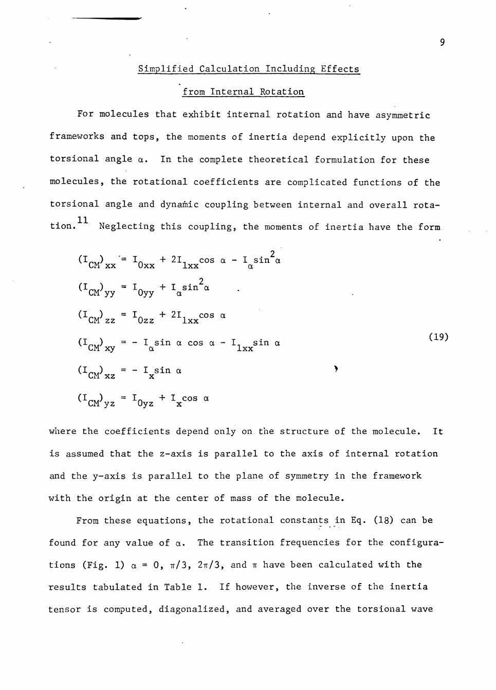
For molecules that exhibit internal rotation and have asymmetric
frameworks and tops, the moments of inertia depend explicitly upon the
torsional angle a. In the complete theoretical formulation for these
molecules, the rotational coefficients are complicated functions of the
torsional angle and dynamic coupling between internal and overall rota
tion. Neglecting this coupling, the moments of inertia have the form
2 (I-,,,) '= I^ + 21. cos a - I sin a CM XX Oxx Ixx a
2 (I„.,) = 1 ^ + 1 sin a CM yy Oyy a
(19)
(I -.) = 1 ^ + 21 cos a CM zz Ozz Ixx
(I„-,) = - I sin a cos a - I, sin a CM xy a Ixx
^^rnJ = - I sin a > CM xz x
CM yz Oyz x
where the coefficients depend only on the structure of the molecule. It
is assumed that the z-axis is parallel to the axis of internal rotation
and the y-axis is parallel to the plane of symmetry in the framework
with the origin at the center of mass of the molecule.
From these equations, the rotational constants in Eq. (18) can be
found for any value of a. The transition frequencies for the configura
tions (Fig. 1) a = 0, 7T/3, 2TT/3, and TT have been calculated with the
results tabulated in Table 1. If however, the inverse of the inertia
tensor is computed, diagonalized, and averaged over the torsional wave

TABLE 1
RIGID.ROTOR ROTATIONAL CONSTANTS FOR CH OH, CH DOH, AND CHD2OH
Coefficient
•'"Oxx
^Oyy
^Ozz
•""Oyz
Io(
I x
Ixx
CH OH
21.279375
20.529336
3.962416
0.0
0.750040
-0.064854
0.0
CH2DOH
23.509368
21.722499
4.999246
1.112117
0.750292
-0.082221
-0.016188
CHD2OH
24.098613
24.448832
6.069590
-1.079241
0.750530
-0.098562
0.015709
CH OH:
I_. = 21.279375 amu-A X i„ = 20.529588 amu-A'
A = 23750.88 MHz
B = 24624.46 MHz
J=0^1 = 48375.34 MHz
a = 0* a = IT /3 a = 27T/3 a = TT
CH DOH:
I ^ = 23.476993 X
I^ = 21.785802
A = 21533.04
B = 23204.61
V = 44737.65
23.124604
22.157666
21861.18
22815.17
44676.35
23.029525
22.295786
21951.43
22673.84
44625.26
23.541744
21.807962
21473.81
23181.03
44654.84
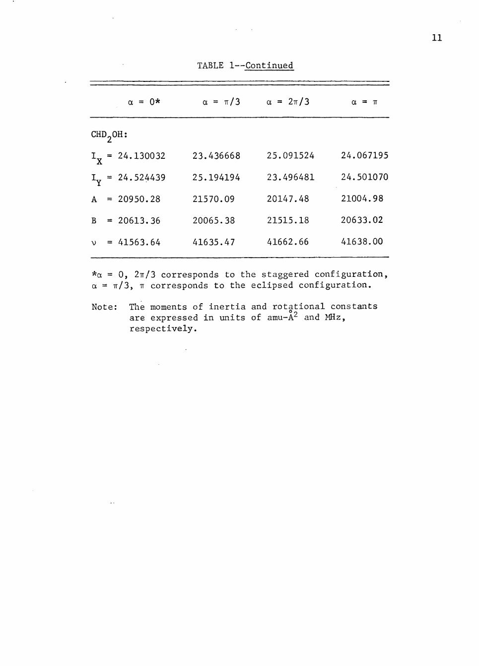
TABLE 1—Continued
11
a = 0* a = Tr/3 a = 2TT/3 a = TT
CHD2OH:
I = 24.130032
1^ = 24.524439
A = 20950.28
B = 20613.36
V = 41563.64
23.436668
25.194194
21570.09
20065.38
41635.47
25.091524
23.496481
20147.48
21515.18
41662.66
24.067195
24.501070
21004.98
20633.02
41638.00
*a = 0, 2TT/3 corresponds to the staggered configuration, a = TT/3, TT corresponds to the eclipsed configuration.
Note: The moments of inertia and rotational constants are expressed in units of amu-A' and MHz, respectively.

12
functions, an average value for the effective rotational Hamiltonian may
be found for each of the torsional substates.
The inverse, _y_, of the inertia tensor may be found in at least two
ways. In one method the inertia tensor is diagonalized to second order
which yields new diagonal elements
( I ) '
where 3j Y ~ x, y or z. The denominator in the suTnmation contains
2 a-dependent terms (cos a and sin a) which may be expanded in a trigono-
. 1 2 metric series.
2 If, however, the coefficients of cos a and sin a are small
com.pared to the constant terms in (I^T,,)OD» ^^^ principle moments of CM pp
inertia are approximately given by
(I ) ^ I ^ n ) +J —CMlil . (21)
If the a-dependence is small, the inverse of the inertia tensor can then
be computed by expansion in a Newman series and the resulting elements
averaged over the torsional wave functions. The results of calculation
of the rotational constants by this method for CH2DOH and CHD2OH are
given in Table 2.
In an alternate method the inertia tensor is written as the sum of
a constant tensor and an a-dependent tensor:
I = IQ + 1(a) . (22)
The inverse of I is then found by expansion in a Ne^^an series. If y^ is
defined as

13
TABLE 2
AVERAGED ROTATIONAL CONSTANTS FOR CH DOH AND CHD OH
Method 1:
CH2DOH
y = 0.02126816 - 0.00002929 cos a + 0.00070340 sin^a XX u = 0.02328748 - 0.00003922 cos a + 0.00005170 sin^a yy y = 0.10119189 + . . . • zz
y = 0.00073330 sin a cos a - 0.00005170 sin a xy
y = 0.00016243 sin a cos a - 0.00036518 sin a xz
y = 0.00523472 + 0.00035036 cos a - 0.00001427 sin^a ^yz
u = 0.02126816 - 0.00002929 cos a + 0.00033860 sin^a x
y = 0.02293416 - 0.00008631 cos a - 0.00033310 sin^a y
V = 44694.06 IBz
V = 44666.66 MHz
V = 44721.46 MHz
CHD OH
2 y = 0.02074812 + 0.00002705 cos a + 0.00066712 sin a XX
2 y = 0.02060521 - 0.00002510 cos a + 0.00003780 sin a yy
u = 0.08300174 + . . . zz •'• " •
u = 0.00063795 sin a cos a - 0.00029717 sin a xy
u =-0.00002031 sin a cos a + 0.00030674 sin a xz
2 u = 0.00351695 + 0.00015881 cos a - 0.00011110 sin a yz

14
TABLE 2—Continued
y = 0.02074812 + 0.00002705 cos a + 0.00413146 sin^a x
y = 0.02041569 - 0.00004218 cos a + 0.00351609 sin^a
VQ = 45482.44 MHz
v^ = 43810.09 MHz
V = 47154.79 MHz
Method 2:
y = 0.02126808 - 0.00002929 cos a - 0.00067753 sin^a XX
y = 0.02329341 - 0.00003838 cos a + 0.00080975 sin^a yy y = 0.10121542 - 0.00048861 cos a - 0.00005542 sin^a zz
y =-0.00074694 sin a cos a - 0.00003437 sin a xy
y = 0.00001609 sin a cos a + 0.00035753 sin a xz
y =-0.00524122 - 0.00105516 cos a + 0.00018061 sin^a yz
y = 0.02126808 - 0.00002929 cos a - 0.00095518 sin a X
2 y = 0.02292658 - 0.00003838 cos a + 0.00104722 sin a y
VQ = 44728.66 MHz
V = 44764.01 MHz
V = 44693.23 MHz
CHD2OH
2 y = 0.02074812 - 0.00002705 cos a - 0.00064512 sin a XX
2 y = 0.02060584 + 0.00002468 cos a + 0.00063785 sin a yy

15
TABLE 2—Continued
y = 0.08297534 + 0.00033024 cos a - 0.00004192 sin^a zz
y = 0.00064224 sin a cos a + 0.00002626 sin a xy
y =-0.00011005 sin a cos a + 0.00029974 sin a xz
y = 0.00357968 - 0.00013531 cos a - 0.00010944 sin^a yz
y = 0.20748120 +'0.00002705 cos a - 0.00002730 sin^a X
y = 0.02019494 + 0.00007222 cos a - 0.00002911 sin^a y
VQ = 41367.45 MHz
v^ = 41402.26 MHz
V = 41332.64 MHz

16
-1 '0 2 "0 ln = T ^n » (23)
then
H = IJ - 2jj^(a)jj^ + 4jy^(a)_iJ^(a)_y^ + . . . . (24)
The matrix _y_ can then be diagonalized approximately to second order with
the a-dependent terms in the denominators neglected. That is,
2
Then the y may be averaged over the torsional motion which results in p
three equally spaced lines, one for each torsional substate. The results
of calculations of the rotational constants for CH^DOH and CHD^OH are
also in Table 2..
Stark Effect
The Stark effect is the change in the energy levels of a molecule
when the molecule is subjected to an external electric field. The rota
tional spectrum for a molecule with an electric dipole moment would be
expected to be modified when the molecule is in an electric field since
the field exerts a torque on the molecular dipole moment and can thereby
change the rotational motion.
The Stark energy in molecules is generally small compared to the
rotational energy. This suggests that quantum mechanical perturbation
theory be employed to find what effect an electric field has on the spec
trum of a molecule. Most of the results of this section are based on the
13 14
simplified development found in standard references. *
This calculation is initiated with the Hamiltonian operator for a
molecule in an electric field o which is arbitrarily chosen to be along

17
the Z axis of the space-fixed coordinate system. The Hamiltonian may be
written as
H = H° - jj. . £. + Hp (26)
where H is the unperturbed Hamiltonian operator, jj is the permanent
electric dipole moment of the molecule and H is a polarizability term
which is negligible for molecules with a permanent dipole moment. The
first-order energy is simply the average of the interaction energy over
the quantum-mechanical state:
AE(« = - f i)*(]i • _£_)i|jdv = - fv^]i£ cose i|;dv (27)
where 0 is the angle between _y_ and the field _6_. For a symmetric-top
molecule, the first-order energy correction is
.^(1) c MK ,oQx
^^ - - ^ J(J + 1) • (2^^
Transitions may occur with selection rules AJ = +1, AK = 0, AM = 0
or +1. The observed frequencies for a transition J J + 1 are given by
E - E so that when AM = 0
V - 2B(J + 1) + j^j + i)(j + 2)h
and when AM = HHl,
- 9i.rT + n + (2M+ J)Kyg V - 2BU + i; + j^j + i)(j + 2)h
2MKy€. ^29)
(30)
where M corresponds to the initial or J state.
A calculation to second order takes into account the small changes
in the molecular wave function due to the field. The resulting energy
may be written as

18
n ' n n '
where E and E , a re the energies of the undisturbed s t a t e s n and n ' n n ^
r e s p e c t i v e l y , and y , i s the z component of the d ipole moment matr ix
element between the s t a t e s n and n ' . For a syitmietric-top molecule, the
matr ix elements are zero for a l l s t a t e s except J = J ' o r J = J + l when
M = M' and K = K' s ince jj i s always along the symmetry axis for a t rue
syiiraietric t op . Thus, the sum involves only two terms between s t a t e s
J ' = J + 1 and J ' = J - 1, which gives
^£^2) ^ M^e^ / ( J ^ - K 2 ) ( J 2 - M ) _ r(J + 1)^ - K 2 ] [ ( J + 1)2 - M^]) ^32)
2Bh ( j 3 ^ 2 j - i ) ( 2 J + 1) (J + 1)^(2J + 1)(2J + 3) ^
which for K = 0.simplifies to
.^(2) _ ^^E^ J(J + 1) - 3M2 ^^ 2hBJ(J + 1) (2J - 1)(2J + 3) ' ^^^^
and for the special case where J = 0,
The observed frequency for the transition J = 0 -> 1 is given by
^ ° ^ 15h(I^A) • "5)
Although none of the methyl alcohol molecules are strictly syiranetric
tops, the error introduced by using the syiranetric-top Stark energy is
small. However, Eqs. (33), (34), and (35) are only applicable for the
component of the molecular dipole moment parallel to the apparent
"symmetry" axis.

19
Line Shape and Intensity
The development of the intensity formula for microwave absorption
can be made from the Einstein transition coefficients. For non-
degenerate quantum states J and J' in absorbing molecules, the proba
bility p f that a transition J -> J' will be induced from the lower
state J to the higher one J' by radiation of frequency v,,, and density
p(Vjj,) is given by
where B , is the Einstein coefficient of induced absorption. The number
of molecules per cubic centimeter N , undergoing such a transition in
unit time is
in which N is the number of molecules in the state J. The number of
particles undergoing the reverse transition in unit time is similarly
in which B , is the Einstein coefficient of induced emission. The
Einstein coefficient of spontaneous emission, A^^^,, has been neglected
because at microwave frequencies A^^^, « B^^j,. Since the induced emis
sion and the induced absorption are coherent with the radiation p(Vjjt),
the net loss of energy density of frequency v^j, in time At is
= -hVjj.(Nj-Nj,)Bj_^j,p(Vjj,)At (39)

20
since B^ , = B
The absorption coefficient a is defined as -(1/P)(dP/dx) where P is
the power and -dP/dx is its rate of loss with distance through the
absorbing species. Since P = constant x p and dx = cdt,
where c is the velocity of electromagnetic propagation. If thermal
equilibrium is maintained, the Boltzman distribution law holds and
-hv ,/kT (Nj,/Nj) = e ^ . (41)
Therefore,
-hv /kT hv__ Nj - Nj. = Njd - e ) = N - # . (42)
The last approximation holds very well since at microwave frequencies
f * 16
hv << kT for T = 300*'K. From quantum mechanical perturbation theory,
V J ' ^ \ (JU|J')^ (43)
h
where (JIJJ^IJ') are the matrix elements of the components of the dipole
moment jj which causes the transition. By using Eqs. (40), (42), and (43),
the absorption coefficient becomes 3 2
8TT V , N «
Equation (44) holds for a single, discrete frequency v^^,. Because
the line has a natural line width and is also broadened by the Doppler
effect, collisions and other phenomena, the transition J J* results in
absorption over a band of frequencies. Hence the absorption coefficient

21
must be modified. The absorption coefficient a for any frequency v in
the band is defined as
% = VJ'^^^'V
or 3 2 8TT- V N
a = V
ckT - (j|ji|j')^S(v,VQ) (45)
where S(v,v„) depends upon the shape of the absorption line and v^ is
the frequency of maximum absorption.
The total microwave power of frequency v absorbed in a length X can
be obtained by integration:
\ ^ Jo a dx V
or
In — = - ax 0
Therefore,
p = V -ax (46)
where P^ is input power to the cell and P is that remaining after trans
mission a distance x through the absorption cell.
The line shape factor S which is attributed to pressure broadening,
i.e., collisions between molecules, is given by "the Van Vleck-Weisskopf
15 expression
V ^ 'V = .V
0
Av 2 2
(VQ - V) + AV
-f Av 2 2
(v„ + v) + Av (47)

where
22
Av= 1 2TTT
T = the mean time between collisions,
VQ = the peak resonant frequency.

CHAPTER III
THE SPECTROGRAPH
The spectrograph used to obtain the measurements listed in this
thesis is a conventional Stark-modulated microwave spectrograph patterned
after one described by McAffe, Hughes, and Wilson.''"' A block diagram of
the spectrograph is shown in Figure 2. Details of construction and
operation of the individual waveguide components can be found in the
18 literature. The uses of these components in this system are described
below.
The spectrograph, as designed, can be operated from 8.4 GHz to
50 GHz; however, for the measurements listed in this thesis, a frequency
range of only 40 GHz to 48.4 GHz i<ras required. Three reflex klystrons,
listed in Table 3, provided electromagnetic radiation for this frequency
range.
TABLE 3
THE KLYSTRONS USED IN THIS WORK
Klystron Tube Type
40V10
45V10
QK294
M^mufacturer
OKI
OKI
Raytheon
Frequency Range (GHz)
37.5-
42.5-
41.7-
-42.
-47,
-50,
,5
.5
.0
The reflex klystron operates on the principle of velocity iv.odula-
Li.on of an electron beam by a resonant cavity. The velocity-mo;Uil.ited
23

24
T3 0) C
H
Q) • H <+-i • H rH
a, g 0) v-l
•H I
o
U
•H
I
QJ -1
<X> 0 cr
t/)
(U > n3
: 2
U O u cd 5-1 Q)
a
U u cd
rC
o
v-l 0)
T3 ^1
o o OJ PS
r
cN
QJ U 3 60
•H P-i
^ O. CC VJ W) u }-l 4-t
a (U D-
C/2
QJ x: H
J^

25
electrons form bunches, are reversed by a reflector, and sent back
through the cavity in such a phase as to give up energy to the oscil
lating field.
Although the usual reflex klystron generates relatively low power,
at best a few hundred milliwatts, it has two features, ease of tuning
and purity of its spectrum, that make it a very satisfactory radiation
source for microwave spectroscopy. The radiation produced by the kly
stron is monochromatic except for noise that arises from voltage and
thermal fluctuations.
The klystron frequency can be varied by mechanical tuning over
approximately a 5000 MHz range or by electrical tuning over approximately
100 MHz. The frequency can be swept electrically by applying a modu
lating voltage to the reflector.
Both methods of changing the klystron frequency are used depending
on the type of information sought. \^en the system is used as a spec
troscope, the frequency of the klystron is varied electrically by a
variable peak-to-peak sawtooth voltage. In this case the spectral line
is displayed as a pip on the oscilloscope trace as indicated in Figure
3. The horizontal sweep of the oscilloscope is synchronized to the
frequency modulation of the klystron. When the system is used as a
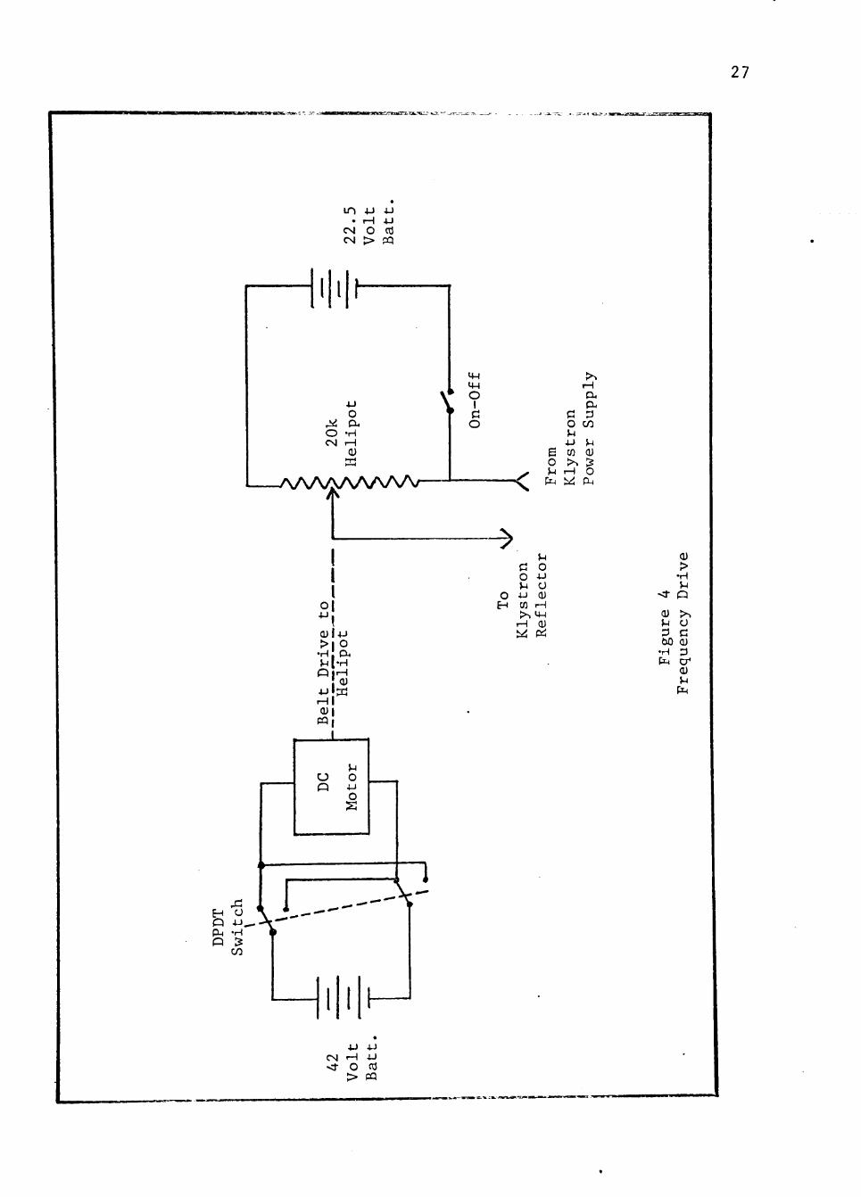
spectrograph, the frequency of the klystron is changed very slowly by
changing the voltage on the reflector with a helipot driven with a
motorized drive. A schematic diagram of the unit is shown in Figure 4.
The spectral line is displayed as a deflection of the writing pen on a
strip chart recorder as shown in Figure 5.

26
" r~'^'rrr^rrrr7^i-\Tnn-Trrmrm
i'.*--V*.''
I .-...^
1
.If'--^, •• y^ ,- »< t * 1
fc.^'
44,713.86MHz Line of CH DOH
Stark Voltage: 400 Volts Splitting: 2.05MHz
fi
• \ I . \
i \
44,713.86MHz Line of CH DOH
Stark Voltage: 700 Volts Splitting: 6.31MHz
Figure 3 Oscilloscope Display of a Spectral Line
in -P 4-) • r-H J-)
eg o CO CM > pq
27
4-)
o O -H
QJ
-AAAAAAAAAr
o I
o
<
(X
C 3 O C/D M iJ >-<
g W QJ O > . [2 M iH O
P4 ^ PM
^
O H
J-i C O O -U >-i O 4-J Q) CO iH
iH 0) 1^ P^
1
CM - H
CO
-C^^
< t
Q) M 3 Ml
•H fx
> •H 5-1 Q
>. O C QJ D cr 0) >-i
|i<
4-J 4-) CNI r H 4-J <J- O cd
> CQ

28
CH DOH
44,558.87MHz
Stark Voltage: 600V
A: Unperturbed Line
B: Perturbed Line
C: Frequency Markers
Figure 5 Chart Display of a Spectral Line

29
The spectrograph is useful for observing very weak absorptions
because of its greater sensitivity. The spectroscope on the other hand
is useful for preliminary investigation of a frequency interval since
quicker scanning is possible.
Distortion of the line shape can occur if the frequency of the kly
stron is changed too rapidly. To minimize this effect, an electrical
modulation frequency of 12 Hz is acceptable with oscilloscope display.'
The frequency sweep varies from approximately 100 I"iz/second to
500 MIz/second depending on the modulating voltage provided by the
internal modulator in the klystron power supply. For chart display,
sweep speeds requiring several seconds for the frequency to change 1 MHz
are used. All data reported in this thesis was taken at a sweep speed
of approximately 0.05 MHz/second.
The klystron power supply provides the proper voltages and currents
for the operation of the klystron. Figure 6 is a block diagram of the
FXR Model 815C power supply used for this work. The 815C supplies four
variable DC voltages that are applied to the filament, beam, reflector,
and grid of the klystron. Typical operating voltages and currents for
the OKI klystrons and the accuracies to which they can be set are:
filament, 6.3 + 0.1 volts at 0.7 amperes; beam, 2,300 + 6 volts at
20 milliamperes; reflector, -170 +2.5 volts at 0 to 50 microamperes;
and the grid, -140 +1.5 volts at 0 to 50 microamperes. All voltages are
referenced to the cathode which is 2,300 volts below ground potential.
The regulation of these voltages for an input voltage of 105 to 125
volts are: filament, 1% line; beam, 0.005% line and load; reflector,
0.005% line; and grid, 0.005% line.

30
• nn -~r ,nTnn- i fc -nTT- r i > ' r wi.iw i—i i i _ i i_
o u
o -u H CO
QJ • S * 'T3 13
r-H CO m -H O •H QJ QJ M C PM pq Pi" O <d
c O V-i • P CO >^
rH ;^
4-» d QJ
e CO rH •H pt.
> rH CU P-3
CO
4J C! >% QJ rH 6 cu CO a .
r-i a • H CAJ fl^
<
i - (
QJ 60 CO 4-> rH o > rC 60
M
«
QJ 6
•H H
!> CO
rH QJ Q
- \ - \ -4J
QJ
lam
•H
» ^
QJ fL, fi
•H hJ
QJ 60 CO
O >
60 •H
rH a ex
CO
QJ
QJ :s M O 60
•H fi ^ O
>-i +J CO >^
rH 1^

31
The radiation produced by the klystron is propagated do\<m. a
rectangular waveguide of inside dimensions 0.220 x 0.105 inches to a
directional coupler where 1/100 of the power is diverted from the main
waveguide into a modified crystal mount for the measurement of the fre
quency. The power remaining in the main waveguide then enters a
wavemeter used for frequency measurement. The radiation then enters an
attenuator which is primarily a power regulator used to prevent exces
sive power from the sample region. The attenuator also serves to
isolate the klystron from the load impedance. The absorption cell which
contains the gas sample is a frequency-dependent load, whereas the
attenuator is a non-frequency dependent load and can be used to isolate
the two parts of the system. A highly frequency-dependent load can
cause sharp cusps or discontinuities in the klystron output which under
some conditions may be mistaken for spectral lines. That the klystron
output is' much greater than is necessary to observe an absorption causes
the attenuator to dissipate most of the power leaving little of the power
to be effected by changes of impedance in the cell.
The radiation leaves the attenuator and passes through a transition
to the absorption cell. The transition is simply a transformer from the
smaller waveguide that precedes it to the larger x^aveguide from which
the cell is made.
The absorption cell for the gas is made from a section of brass
X-band waveguide of length ten feet and inside dimensions 0.900 x
0.400 inches. The Stark electrode is installed in the center. Figure 7
shows the detail of the construction of the cell. The Stark electrode
is a strip of flat soft brass 0.840 inches wide, 0.035 inches thick, and
9 feet 9 inches long. The electrode is supported by tv;o teflon strips so

32
60 fi
• H rO
D H U QJ
a a o u
6 Q) 4J CO >. CO
e d 3 O CO > CO CO CO
r-{
p-CO
u 6 D :3
o CO
60 >
o 4J >._•
CO 4-1
o PLI
g d 3 O CO >
CO u CO
rH QJ
CJ
fi o
•H 4J
Q) CO
M • CO > o ^
v-l r^ O
CO QJ rO
u < fi 60 QJ
•H ^ PM 4 J
M-l O
rH •H CO 4J QJ
Q
«ntMue<WN •v«'4-a: •^^i^s^jss'W-^-'-^T * am

33
that it is parallel to the broad side of the waveguide and divides the
cell into two equal parts. The two teflon strips have dimensions 0.394
inches by 0.0625 inches, 9 feet 9 inches long. A groove, 0.035 inches
wide and 0.034 inches deep, has been milled down the entire length of
each strip. The strips were placed along the narrow side of the wave
guide to hold the electrode in place. Electrical connection to the
electrode is made by a wire soldered to its edge at one end and passing
through a Kovar tube supported in a Kovar side tube by a glass bead.
This provides both electrical insulation and a vacuum seal for the connec
tion. The other end of this wire is soldered to the center connector of
an SO-239 coaxial receptacle. The vacuum connection to the cell is made
through a number of small holes drilled in the center of the broad side
of the waveguide. A cap with a larger hole and a short piece of copper
tubing soldered to it is soldered over the holes in the waveguide.
Copper tubing connects the cell to the vacuum system. The ends of the
cell are made vacuum tight with thin mica windows mounted in a thin
copper plate which are mounted to the flanges of the cell with an 0-ring
between them. The vacuum system consists of a gas handling system, a
diffusion pump, and a mechanical forepump. The system is capable of
-3
obtaining and holding a pressure of less than 10 Torr.
After passing through the cell, the radiation enters a second
transition follovjed by a tunable crystal mount in v/hich a 1N53 microwave
diode serves as the microwave detector. The tunable crystal mount has
an increased crystal output over an untuned type for a small frequency
range. A 0-50 direct current microammeter is used to measure the average
current passing through the crystal and serves as a means of measuring
the power passing through the cell. The radiation power is roughly
34
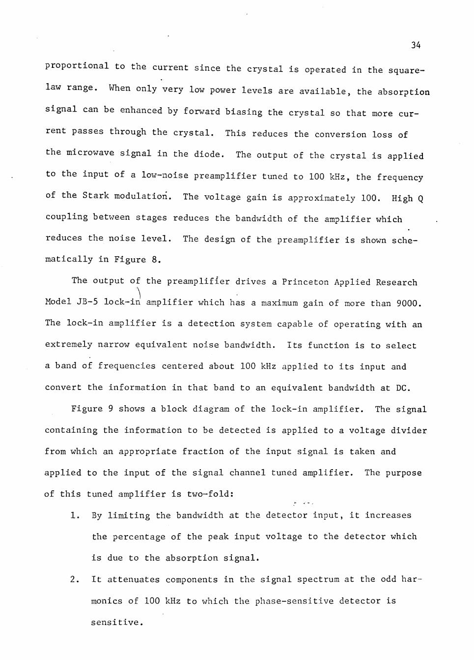
proportional to the current since the crystal is operated in the square-
law range. When only very low power levels are available, the absorption
signal can be enhanced by forward biasing the crystal so that more cur
rent passes through the crystal. This reduces the conversion loss of
the microwave signal in the diode. The output of the crystal is applied
to the input of a low-noise preamplifier tuned to 100 kHz, the frequency
of the Stark modulation. The voltage gain is approximately 100. High Q
coupling betx een stages reduces the bandwidth of the amplifier which
reduces the noise level. The design of the preamplifier is shown sche
matically in Figure 8.
The output of the preamplifier drives a Princeton Applied Research
Model JB-5 lock-in amplifier which has a maximum gain of more than 9000.
The lock-in amplifier is a detection system capable of operating with an
extremely narrow equivalent noise bandwidth. Its function is to select
a band of frequencies centered about 100 kHz applied to its input and
convert the information in that band to an equivalent bandwidth at DC.
Figure 9 shows a block diagram of the lock-in amplifier. The signal
containing the information to be detected is applied to a voltage divider
from which an appropriate fraction of the input signal is taken and
applied to the input of the signal channel tuned amplifier. The purpose
of this tuned amplifier is two-fold:
1. By limiting the bandwidth at the detector input, it increases
the percentage of the peak input voltage to the detector which
is due to the absorption signal.
2. It attenuates components in the signal spectrum at the odd har
monics of 100 kHz to which the phase-sensitive detector is
sensitive.

35
I—
H H "
i n " * * — N A A T rH ^ -t- -H
-,—II—u ^Hl
in
U >-'.
in
XMJ'XMJ tUSU
til'
i n
T. L T cs o o
c? o in CN
c? o o in
o
rujD
t i l
in CN
rujUg
o in
QJ • H
00 6 CO
QJ QJ u u fi p-l 60
•H Q) P^ CO
•H
O
I
O
it-7aTT-T-3 '.les^msm w i jiwrir ^

-'-rzv *r.yia-.-i--y:.^^. >. TJ.^J .^^•v^.j.z- »ny-^,-^^T>^^rTE•.y*.^ p.^-twf '" ilTTF*-p ffftH
36
Signal Input
>
Signal Level
>-
Tuned
Amplifier
Q=25
Overload
Indicator
Phase-Sensitive Detector
Phase
Shifter
Reference Reference Level
Tuned Amplifier Q=25
Amplitude Limiting
Positive Feedback
Netx ork
DC. Amplifier Lo-pass Filter
A Output
»W.'*TT-ir_; iTTTT
Figure 9 Lock-in Amplifier
TT'^^'Wr- TCMt^iflBirBI wswtximi^^'CP- « . auawfc sr'wi>-*jwtfS.a.^JirtMtt'r:'y^ ra?«c wK'^aTr n-TiTwnr'iii''H

37
The output of the signal channel amplifier is applied to the input
of the phase-sensitive detector. This is essentially a device which
mixes the signal frequencies with a variable phase 100 kHz sine wave to
produce corresponding sum and difference frequencies at its output. The
100 kHz sine wave is produced in the reference channel amplifier and is
synchronized with the modulation applied to the Stark electrode in the
absorption cell. A low-pass filter at the output of the phase-sensitive
detector rejects the high frequency components corresponding to the sum
frequencies and passes those of the difference frequencies that lie with
in its pass-band. In particular, the difference frequency due to
components of the signal at the reference frequency is DC. Components
of the signal spectrum differing from the reference frequency by more
than the cut-off frequency of the low-pass filter will be attenuated by
it. Consequently, the output from the low-pass filter will be due to
that portion of the signal spectrum which lies within a band of fre
quencies about the reference frequency determined by the pass-band of
the filter. The distortion of the line shape due to sweeping the kly
stron frequency too rapidly arises from the fact that some of the
information lies at frequencies outside the pass-band of the filter.
A mixer of this type is called a phase-sensitive detector since the
DC output produced by it from a signal at the reference frequency is
proportional to the cosine of the relative phase of the signal and the
reference.
The output of the lock-in amplifier is used to drive the writing
pen of a Texas Instruments 1 milliampere rectilinear 6 inch chart recorder
when the system is used as a spectrograph. \'^en the system is used as a
38
spectroscope, the output of the lock-in amplifier is applied to the
vertical plates of an oscilloscope.
A Stark-modulated spectrograph has the advantage over a non-Stark
modulated spectrograph of being considerably more sensitive without
losing convenience of operation. Two forms of Stark modulation are
coiranonly employed: sine wave and square wave. High voltage sine wave
Stark modulation uses a much simpler generator than is required for
square wave modulation since the capacitance of the cell, 1300 pF for
the cell used in this work, can be incorporated into an L-C network tuned
to the modulating frequency. Square wave modulation requires the
generator to charge and discharge the cell rapidly which, for acceptable
waveforms, means that there is a peak current of several amperes flowing
through the switching tubes.
Although sine wave- modulation is easier to produce than square wave
modulation, square wave modulation is employed in most high sensitivity
spectrographs. With square wave modulation, there are two electric
fields produced in the cell: one that is zero and one of high intensity.
This gives rise to two distinct spectral lines: the perturbed and the
unperturbed lines. When sine wave modulation is employed, there is no
constant field for any arbitrarily small period of time which results
in the broadening of the spectral line.
Two characteristics that an acceptable square wave must have are a
relatively flat top and a baseline that does not drift away from ground
potential. These qualities depend on the frequency response of the
generator.

39
Figure 10 is a block diagram of the generator used in this work.
The output of the 200 kHz oscillator drives a Schmidt trigger at 100 kHz.
The resulting square wave is differentiated with the result that voltage
spikes appear at the output. These voltage spikes are amplified and
clipped and used to control the switching tubes that charge and discharge
the cell. The clamp tube prevents overshoot of the square wave during
discharge. The resulting square wave has a variable peak-to-peak voltage
from about 5 volts to more than 2000 volts. The operation of the square
19 wave generator is discussed in more detail by Hedrick.
The frequency of a spectral line is determined in a manner similar
to that described in reference l7. The technique depends on the accurate
calibration of a conventional communications receiver to yield the
difference between the unknown frequency and the known harmonic of a
standard frequency. This is most conveniently done using a microwave
standard. A block diagram of the frequency measuring system is shown in
Figure 11.
The heart of the microwave frequency standard is the oscillator to
which all measurements are referenced. A Hewlett-Packard Model 101-A,
1 MHz oscillator, a high-stability, crystal-controlled oscillator pro
viding low-distortion 1 MHz and 100 kHz outputs, is used as the frequency
o
standard in this system. Long-term stability of 5 parts in 10 per week
is attained by careful design of the oscillator and by housing a high
quality crystal in a constant temperature oven.
The 100 kHz output of the oscillator drives a General Radio Type
1112 Standard Frequency Multiplier chain. This system provides outputs
of 1, 10, 100, and 1000 MHz. The output of the 10 MHz multiplier drives
a second multiplier chain with outputs of 20 and 40 MHz. The frequencies

40
u
.
5-1
erat
o
c QJ o QJ > CO
S 5-1 CO 0 cr
C/3
"1
rC O
O QJ ,
•H fi —<>-^ H
C/3
t ^ O Q) 5-1 4J 43 QJ •H fi > ^ b^ -r-i
C/2 5-1 Q
r u QJ P^ CX
•H rH CJ
J >-( QJ
•H 1+-I M •H M rH H &.
1 t 1 u u o QJ 4-1
m CO <4H ' H •H 4-1 Q fi
QJ /
1 QJ CO 60
•H 5-1 Q CO
o
t
& g CO
rH
u
1-5-( QJ Cu
a. •H rH
o
t w QJ •H «4H •H > r-l M ex 4 t
1 V-i 5-1 O QJ +J
M-l CO U-i -H •H 4-» Q fi
0)
r r }^ QJ
•H 14-1 •H H rH P4
-h 4-) M X) QJ •H 60 g 60
^ -H a 5-1
lO H
t 5-
Q) QJ - f i 13 O O
^ r-4J r-CO O
O f n
N
-. — —
5-1 QJ
•H M-( •H H rH M PH
g
t +J 5-1 T3 QJ •H 60 g 60
^ -H O 5-1
CO H
t U
QJ QJ X) [5
o o rC rH 4J rH CO O
U P4
- ^ N 1 P^ rH 5-1 J^ "H O O O 4-» O CO CO r^j O rH
CO
g 5-1 O
4 H QJ > CO
5-1 QJ
a. ex
•H
^1 QJ P-Cu
•H T-H U
L
•H
M-l • H Q
Q) • H M-l • H
r
T-\ (X CO g u <
• H CX M
H 5-1 QJ
•H U-t •H rH CX
4-) U X) QJ •H 60 g 60
^ -H O 5-1 cn H
QJ ^1 T3 QJ O 15
^ O 4-1 rH CO r-H u o
^ ^ '' - y
IK ,zi *". TT,'«r-jrri^i^'zut»i
o CO
• H U CO
o
L L
L
L
r f L
f 5-t O 4-1 CO V-i
O QJ H C
QJ QJ O V-i fi QJ 60 >
•H cO
QJ 5-1 CO : i
CO
"Xy -N3^ Z\.

» SCL:* aj^auwjifwfc',: ^
41
w QJ
• H N r-\
a a. O - H 4-)
rH rH fi s ^
5-1 0)
0 M
Hz
tip
li
O rH
. , 1 /
• %
>
*
'
> X) o 5 fi CO QJ 5-1
T3 fi QJ fi cr X CO QJ - H 4J n s CO pL,
i
-1 QJ
• H N r-{
3 .^ 4-1
O r-\ fH fi
1 1
u QJ
N - H W rH S P-
• H r H 4J
r H fi 2 - k
M X) o
N ^-t 4-1 W CO rO ^ T3 rH
fi rH O CO - H O 4-1 O r H CO CO
o
1
4 J 5-1 '^1 QJ QJ ^ > 5-1
W CO
S
^n
k
u QJ
•H N rH
a P-S -H 4J O rH
> t
5-1 QJ
N - H
S rH 1 ^ t i l
• H O 4J < j - r H
:^ S
^
tor
Op
era
» *
r
5-1 QJ Q)
r H - H > CO r H CO 5-1 4-1 a > QJ CO -H O X >> 4J V- l -H 5-1 rH a S
U fi -H
ss . I
5-1 pq QJ X) rH
P< O fi Csl O
CJ
^ 1
QJ X ) •H
fi 3 •H 60 CO QJ
S > CO
: 2
^ >
«
1 .
CO 5-1 fi QJ
•A r-K 'p. rH CO -H rH rH QJ o in a o a
r^
\ f
1 o
T->. QJ
r H P J •H O o a CO CO
o
r H J-^
QJ 5-1 fi 60
•H Pi^
g QJ 4-1 CO
>> CO
4J
fi QJ g QJ 5-1 •:i CO CO QJ
S > O fi QJ fi cr QJ 5-1
PLI

42
of 10, 20, 40, 100, and 1000 MHz are fed by coaxial cable to a mixer in
which any combination of frequencies can be mixed with the 1000 MHz
signal. A schematic diagram of the mixer is shown in Figure 12. The
output of the mixer is applied to a 1N53 crystal diode harmonic
generator and microwave mixer. The unknown frequency and the standard
frequencies are mixed producing a heterodyne frequency that falls within
the range of the receiver. The crystal mount was modified as shovm in
Figure 13 so that the diode would perform as a harmonic generator and
microv7ave mixer.
The unknown frequency is determined as follows: Let the unknown
frequency be denoted by F. Mixing F with a harmonic of 1000 MHz, produces
sum and difference frequencies. The difference frequency lies between 0
and 500 MHz. This frequency is in turn mixed with a harmonic of either
100 MHz or 40 MHz, the choice of which depends upon whether the resulting
frequency lies within the range of the receiver. These results can be
stated in algebraic equations as follows:
F = 1000 n -1- 100 m + F„ K
or
F = 1000 n -f 40 ra + F^
where n and m are integers and F_, is the frequency indicated by the
receiver. The integers n and m and the sign before 100 m or 40 m are
determined from the frequency indicated by the wavemeter which is dis
cussed below. The sign before F^ is determined by observing the direc-
tion in which the frequency marker on the oscilloscope moves when the
frequency of the receiver is changed. If the receiver is tuned to a

43
j : -vr r •7j3Kr^ tJM-g-MI».TJ.K>»r'a -»-.i-arc-i»—tramr^Ti -
fi a,
m 13
4-1 fi P-fi
r7:OTr..*gr-7VT.r; jfTTiCr:
N
13 M CO
X l fi CO •M CO
\
fi QJ :i u cr fi QJ p .
u a ^ H
N
O CSJ
3
o <1-
QJ
:i o a. -H
fi o o
H
fi fi o g u Q)
•H g
CS]
o o rH
N
o O O
5-1 QJ
o c
CM QJ rH :i
cr QJ QJ
fi P4 60
•H X) ^ u
CO T3 fi CO 4J CO
Bisj'--

44
higher or lower frequency and the marker moved to a higher or lower
frequency respectively, the sign is "+." Otherwise, the sign is "-."
The frequency marker appears as a voltage spike on the oscilloscope and
is superimposed on the spectral line by using a dual-trace attachment.
I Then the chart recorder is used as the indicator, the frequency markers
appear as a sudden rise in the R.F. power meter on the receiver. When
a frequency marker is received, the event marker on the chart recorder
is triggered manually by the operator. The receiver used for frequency
measurement is a Collins 51S1 which provides markers accurate to 1 kHz
or better at one MHz intervals.
The wavemeter, a mechanical device used to measure the frequency of
the radiation with an accuracy of 0.1%, is a cylindrical cavity whose
dimensions can be varied. The resonant frequencies of the cavity are
given by
(FD)^ = [(cx„ )/7T]^ + (cn/2)^(D/L)^ Jem
where x is the mth root of the Bessel's function, J and n are integers m
representing the number of nodes along 9, r, and z respectively, and c
is the velocity of light. In normal usage L is varied until a resonance
occurs for successive values of n. The interval L is measured with a
micrometer. The solution of the above equation for n = 1 is
2L = c/[f^ - (CX^^/TTD)^]^/^
which may be plotted on a large scale so that the frequency may be found
from L using the chart.

CHAPTER IV
EXPERIMENTAL TECHNIQUE
This chapter is intended to give the reader an idea of the procedure
followed in obtaining the measurements listed in this thesis. It is
assumed that the spectrometer has been set up and has been used pre
viously so that normally one would have only minor adjustments to make.
All electrical components in the system are turned on. In the
square wave generator and klystron power supply, only the filament
supplies are turned on initially in order that the mercury vapor recti
fiers and the klystron filament have sufficient time to rise to operating
temperature.
During this warm up period, all interconnecting cables are checked
and the vacuum system tested for leaks by closing the stopcock to the
diffusion pump and noting the reaction on a thermocouple vacuum gauge.
The high voltage supplies in the_ square wave generator and klystron power
supply are then turned on. The klystron is checked to see if it is pro
ducing radiation by observing the detector crystal current or by varying
the reflector voltage until there is a sharp rise in the beam current.
The entire system is allox\red to rise to operating temperature which takes
approximately 20 minutes. If data is to be taken at dry ice temperatures,
the insulated box surrounding the absorption cell is packed in dry ice.
The reference voltage in the lock-in amplifier is peaked and the synchroni
zation of the oscilloscope trace with the klystron s 7eep is checked. The
frequency at which the klystron is operating is measured with the wavemeter,
45

.46
If the frequency is in the range to be investigated, the search for
spectral lines can be started; otherwise, the frequency must be adjusted.
The gas sample is admitted to the absorption cell to a pressure of
about 10 Torr, the detector crystal tuned for maximum current, and the
Stark modulation increased to several hundred volts. When a spectral
line is found by mechanically tuning the klystron, the system is
optimized by adjusting the attenuator, the fine frequency, phase and •
sensitivity controls on the lock-in amplifier, the sensitivity of the
oscilloscope and by retuning the detector crystal.
After noting some of the characteristics of the lines in the region
on the oscilloscope, the frequency markers are located in relation to
the lines.
After preliminary investigation, a sweep over the region is
initiated so that the weaker absorption lines not discemable on the
oscilloscope display may be observed. Ifhen the general location of each
line has been noted, each line is swept individually to determine its
frequency and Stark effect. The study of individual lines is carried out
-3 -3
at as low a pressure as possible, from 10 to 5 x 10 Torr, while
keeping the noise level well below the signal level. The radiation
density is also reduced so that the sample is not saturated; that is,
an increase in radiation density increases the intensity of the line.
These precautions are necessary to minimize pressure broadening and to
improve the coincidence of the maximum intensity point of the line with
the line itself and improve the accuracy of the frequency measurements.
The study of a line begins by calibrating the receiver. A trial
sweep permits final adjustment of the system so that most of the chart
paper is used and the behavior of the frequency markers may be noted.

47
The Stark effect and the frequency of the line are measured simul
taneously. To measure the Stark effect. Stark modulating voltages of
from 100 volts to 1000 volts at 100 volt intervals are used. Since the
Stark effect is the difference in frequency between the deviated and
undeviated lines, the frequency of both lines must be determined.
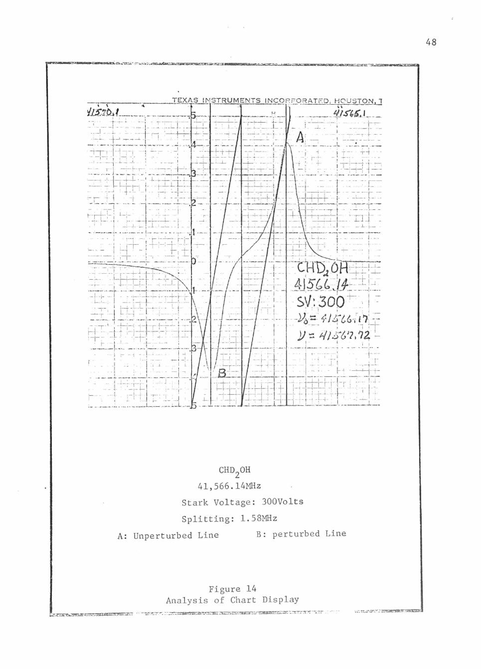
Analysis of the resulting charts yields the desired information.
To determine the frequency of the line or Stark lobe, vertical lines are
drawn through the maximum intensity point of the absorption line and
through the frequency markers on either side of the line as sho n in
Figure 14. A diagonal line is then drawn in the rectangle formed by the
vertical lines through the frequency markers and the edge of the chart
grid. The frequency is then determined by finding the ratio of the grid
lines above the intersection of the diagonal line and the vertical line
through the absorption line to the total number of grid lines across the
chart. Since there are fifty grid lines across the chart, the frequency
of the line is twice the number of lines above the intersection plus the
frequency of the frequency marker to the right of the absorption line.
The accuracy of this method can be estimated as follows. The
intersection of the two drawn lines can be determined to one third of a
division which corresponds to an error of approximately 6.7 kHz. The
error in determining the position of maximum intensity point of the
absorption line, the placement of the frequency marker on the chart, and
any delays that may occur in the system cannot be estimated individually.
However, an estimate of a total error of +23 kHz has been made by
measuring the frequencies of numerous lines that have been previously
reported. These measurements are reported in Appendix II.
48
rai l i^ikssKJZLCit-cz
TEXAS INSTRUMENTS INCORPORATED; HOUSTON. "T
J}s'^S'J
CHD OH
41,566.14MHz
Stark Voltage: 300Volts
Splitting: 1.58MHz
A: Unperturbed Line B: perturbed Line
n?::tTfc3ruB'is!i;3SHBsnnRE:ir.'
Figure 14 Analysis of Chart Display

49
Those lines which have single Stark lobes moving to higher fre
quencies are then studied to determine their relative unsaturated
intensities. Although the relative intensity measurements listed in
this thesis are subject to error, it is believed that they are accurate
to within 15%. Esbitt and Wilson describe a system on which relative
intensity measurements can be made with only a few percent error in
20 the results. The major contribution to error is associated with
multiple reflections in the waveguide and can be reduced substantially
through careful design of the Stark cell and the use of ferrite isolators
at both ends of the cell. Since isolators were not available at the fre
quency required for this work, reflections occurring outside of the cell
could not be avoided. To minimize these effects, relative intensity
measurements were made at several different pressures and at several
different power density .levels.
To determine relative intensities, the gas sample is admitted to the
-3
cell at a pressure of about 5 x 10 Torr and allowed to reach equili
brium which takes several hours. The power density in the waveguide is
assumed to be proportional to the current in the detector crystal so
measurements of two lines are carried out at the same crystal current.
The only difference would arise from a change in conversion loss in the
diode as the frequency changes. Even after taking all measures to
assure identical conditions for the measurements of tx o lines, multiple
reflections in the waveguide can occur causing error in the relative
intensities.

CHAPTER V
ANALYSIS OF DATA
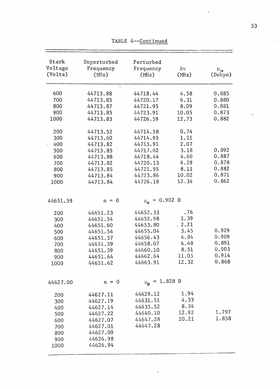
The data needed to identify and assign the spectral lines of CH DOH
and CHD^OH to the J = 0 - 1 transition are frequency, the Stark effect,
and relative intensities of each line. The Stark splittings of those
lines in the partially deuterated molecules that behaved similarly to
those in the normal molecule, i.e., one second order Stark lobe moving
to higher frequencies, are given in Table 4 along with the splittings in
the normal molecule. A comparison of the calculated dipole moment for
each line is possible with the aid of Table 5. The calibration of the
squarewave generator with the J = 0->1, n = 0 transitions in CH OH is
given in Table 6. The dipole moments are believed to be accurate to
TABLE 6
CALIBRATION OF THE SQUAREWAVE GENERATOR*
Stark
Voltage
500 600 700
. 800 900 1000
^Determine of CH OH.
E(48377.60)
(esu/cm)
12.058 14.664 17.200 19.526 22.033 24.470
;d from the J =
E(48372.49)
(esu/cm)
12.183 * *
17.434 19.654 22.044 24.584
0 -> 1, n = 0
E ave
(esu/cm)
12.120 14.664 17.317 19.292 21.646 24.238
transitions
**48377.60 line interferes with the Stark lobe.
50

51
TABLE 4
STARK MEASUREMENTS OF CH OH, CH DOH, AND CHD OH
Stark Voltage (Volts)
48377.09
100 150 200 250 300 350 400 450 500 600 700 800 900 1000
Unperturbed Frequency
(MHz)
MHz n = 0
48376.64 48376.68 48376.76 48376.83 48376.91 48376.94 48376.99 48377.03 48377.09
48377.00 48377.07 48377.07 48377.08
Perturbed Frequency (MHz)
CH OH
48377.35 48377.49. 48377.59 48377.82 48378.10 48378.43 48378.85 48379.37 48379.94 48381.31 48382.90 48384.58 48386.64 48388.86
Av (MHz)
0.28 0.41 0.51 0.74 1.02 1.35 1.77 2.29 2.86 4.23 5.82 7.50 9.56 11.78
Electric Field (esu/cm)
12.058 14.664 17.200 19.526 22.033 24.470
Measured Frequency = 48377.08
48372.
100 150 200 250 300 350 400 450 500 600 700 800 900 1000
60
Measured
MHz n = 0
48372.28 48372.25 48372.31 48372.37 48372.48 48372.52 48372.60 48372.58 48372.63 48372.56 48372.55 48372.57 48372.56 48372.56
Frequency = 48372.
48372.90 48373.03 48373.13 48373.38 48373.67 48374.03 48374.36 48375.02 48375.49
48378.55 48380.17 48382.13 48384.46
.57
0.33 0.46 0.56 0.81 1.10 1.46 1.79 2.45 2.92
5.98 7.60 9.56 11.89
12.183
17.434 19.654 22.044 24.584

52
TABLE 4—Continued
Stark Voltage (Volts)
48257.49
200 250 300 350 400 450 500 600 700 800 900 1000
Unperturbed Frequency
(MHz)
n = 1
48257.30 48257.39 48257.*36 48257.48 48257.45 48257.49 48257.46 48257.48 48257.46 48257.50
Perturbed Frequency
(MHz)
y,, = 0.858
48257.94 48258.20 48258.49 48258.86 48259.18 48259.70 48260.26 48261.49 48262.97 48264.61 48266.50 48268.52
Av (MHz)
D
0.46 0.73 1.02 1.39 1.71 2.22 2.78 4.01 5.50 7.14 9.02 11.04
•1 (Debye)
0.867 0.860 0.853 0.869 0.859 0.854
Measured Frequency = 48257.47
48247.89
200 250 300 350 400 450 500 600 700 800 900
n = 1
48247.48 48247.50 48247.56 48247.61 48247.62 48247.64 48247.71 48247.72 48247.73 48247.72 48247.61
y„ = 0.8f
48248.33 48248.53 48248.83 48249.11 48249.63 48249.93 48250.50 48251.82 48253.20 48254.81 48256.52
J9 D
0.61 0.81 1.11 1.39 1.91 2.21 2.78 4.10 5.48 7.09 8.80
0.867 0.870 0.852 0.856 0.848
Measured Frequency = 48247.72
44713.86
200 300 400 500
n = 0
44713.82 44713.85
CH DOH
y = 0.
44714.62 44714.62 44715.91 44717.02
.0880 D
0.76 1.10 2.05 3.16 0.890
53
TABLE 4 ~ C o n t i n u e d
Stark Voltage (Volts)
600 700 800 900 1000
200 300
. 400 500 600 700 800 900 1000
44651.59
200 300 400 500 600 700 800 900 1000
44627.00
200 300 400 500 600 700 800 900 1000
Unperturbed Frequency
(MHz)
44713.88 44713.85 44713.87 44713.85 44713.83
44713.52 44713.60 44713.82 44713.85 44713.88 44713.82 44713.85 44713.84 44713.84
n = 0
44651.23 44651.54 44651.60 44651.54 44651.57 44651.59 44651.59 44651.64 44651.62
n = 0
44627.11 44627.19 44627.14 44627.22 44627.07 44627.01 44627.00 44626.98 44626.94
Perturbed Frequency (MHz)
44718.44 44720.17 44721.95 44723.91 44726.59
44714.58 44714.95 44715.91 44717.02 44718.44 44720.13 44721.95 44723.86 44726.18
y., = 0.
44652.33 44652.98 44653.80 44655.04 44656.43 44658.07 44660.10 44662.64 44663.91
y„ = 1.
44629.12 44631.51 44635.52 44640.10 44647.28 44647.28
Av (MHz)
4.58 6.31 8.09 10.05 12.73
0.74 1.11 2.07 3.18 4.60 6.29 8.11 10.02 12.34
902 D
.76 1.39
. 2.21 3.45 4.84 6.48 8.51 11.05 12.32
.828 D
1.94 4.33 8.34 12.92 20.21
^M (Debye)
0.885 0.880 0.881 0.873 0.882
0.892 0.887 0.878 0.882 0.871 0.862
0.929 0.909 0.891 0.903 0.914 0.868
1.797 1.858

54
TABLE 4—Continued
Stark Voltage (Volts)
44582.19
200 300 400 500 600 700 700 800 900
44582.20
300 400 500 600 700 700 800 900
44558.87
200 300 400 500 600 700 800 900 1000 1000
44512.59
200 300
Unperturbed Frequency
(MHz)
n = 1
44582.06 44582.13 44582.16 44582.14 44582.18 44582.19 44582.20 44582.17 44582.19
n = 1
44582.16 44582.18 44582.18 44582.22 44582.22 44582.22 44582.20 44582.16
n = 2
44558.78 44558.84 44558.86 44558.8.6 44558.87 44558.88 44558.87 44558.86 44558.88 44558.85
n = 2
44512.52 44512.82
Perturbed Frequency
(MHz)
y„ = 0.
44582.84 44583.41 44584.19 44585.48 44586.79 44588.37 44588.30 44590.15 44592.07
y„ = 0.
44583.42 44584.20 44585.41 44586.80 44588.40 44588.31 44590.15 44592.08
y„ = 0,
44559.56 44560.16 44560.86 44562.06 44563.58 44565.36 44566.96 44569.24 44571.55 44571.68
y, = 0
44513.04 44513.62
879
876
.886
.867
Av (MHz)
D
0.67 1.24 2.02 3.31 4.62 6.20 6.13 7.98 9.90
D
1.22 2.00 3.21 4.60 6.20 6.11 7.95 9.88
D
0.69 1.29 1.99 3.19 4.17 6.49 8.08 10.37 12.68 12.81
D
0.45 1.03
.1 (Debye)
0.909 0.888 0.871 0.866 0.873 0.865
0.895 0.886 0.871 0.865 0.872 0.864
0.892 0.896 0.891 0.879 0.885 0.879 0.884

55
TABLE 4—Continued
Stark Voltage (Volts)
400 400 500 500 600 700 800 900
44511.16
200 300 400 400 500 500 600 700 800 900
44495.86
200 300 400 500 600 700 800 900
44456.47
500 600 700 800 900
Unperturbed Frequency
(MHz)
44512.52 44512.50 44512.54 44512.56 44512.62 44512.60 44512.61 44512.63
n = 2
44511.16 44511.24 44511.20 44511.16 44511.21 44511.17 44511.20 44511.20 44511.20 44511.22
n = 3
44495.74 44495.80 44495.86 44495.86 44495.86 44495.88 44495.86 44495.87
n = 3
44456.46 44456.50 44456.46 44456.48 44456.46
Perturbed Frequency
(MHz)
44514.52 44514.54 44515.64 44515.65 44516.94 44518.51 44520.50 44522.42
y„ = 0.
44511.68 44512.22 44513.14 44513.18
44514.26 44515.48 44517.24 44519.16 44521.00
y„ = 0.
44496.48 44497.04 44497.85 44499.02 44500.38 44501.91 44503.75 44505.72
y„ = 0
44459.74 44461.26 44462.95 44464.84 44466.74
Av (MHz)
1.93 1.95 3.05 3.06 4.35 5.92 7.91 9.83
867 D
0.52 1.06 1.98 2.02
3.10 4.32 6.08 8.00 9.84
.880 D
0.74 1.30 2.11 3.28 4.64 6.17 8.01 9.98
.893 D
3.27 4.79 6.48 8.37 10.27
^1/ (Debye)
0.872 0.874 0.861 0.850 0.869 0.861
0.879 0.858 0.862 0.874 0.862
0.904 0.889 0.868 0.874 0.867
0.902
0.903 0.889 0.893 0.880

56
TABLE 4—Continued
Stark Voltage (Volts)
41669.42
100 200 300 400 500 600 700 800
41653.83
100 200 300 400 500 500 600 700 800
41566.14
100 200 300 400 500 600 700 800
100 200 300 400
Unperturbed Frequency
(MHz)
n = 0
41669.27 41669.38 41669.42 41669.42 41669.42 41669.42 41669.41 41669.42
n = 0
41653.74 41653.80 41653.90 41653.83 41653.81 41653.82 41653.90 41653.84 41653.79
n = 0
41566.14 41566.13 41566.14 41566.14 41566.14 41566.14 41566.14 41566.14
41566.07 41566.17 41566.16 41566.15
Perturbed Frequency
(MHz)
CHD^OH
y,l = 0.922
41669.63 41670.01 41670.66 41671.82 41673.03 41674.83 41676.71 41678.95
yjj = 0.902
41654.01 41654.37 41655.07 41656.01 41657.33 41657.35 41658.97 41660.68 41663.05
y,| = 1.017
41566.34 41566.93 41567.76 41569.04 41570.63 41572.78 41576.09 41577.84
41566.34 41566.84 41567.72 41569.05
Av (MHz)
D
0.21 0.59 1.24 2.40 3.64 5.41 7.29 9.53
D
0.20 0.56 1.26 2.20 3.52 3.54 5.16 6.87 9.24
D
0.20 0.79 1.62 2.90 4.49 6.64 8.95 11.70
0.20 0.70 1.58 2.91
^» (Debye)
0.922 0.929 0.913 0.923
0.909 0.907 0.886 0.908
1.022 1.028 1.010 1.021

•e^Ve^^*«^;g
57
TABLE 4—Continued
Stark Voltage (Volts)
500 600 700
41557.18
100 200 300 400 500 600
41533.60
100 200 300 400 500 600 700 800
41491.29*
100 150 200 250 300 350
41488.09*
100 150 200 250 300
Unperturbed Frequency
(MHz)
41566.14 41566.14 41566.13
n = 1
41557.01 41557.18 41557.18 41557.17 41557.17 41557.18
n = 1
41533.45 41533.54 41533.53 41533.60 41533.59 41533.60 41533.59 41533.60
n = 2
41491.22 41491.23 41491.26 41491.31 49491.29 41491.29
n = 2
41488.00 41488.03 41488.04 41488.08 41488.08
Perturbed Frequency (MHz)
41570.47 41572.71 41575.18
y„ = 0.
41557.41 41557.75. 41558.42 41559.37 41560.55 41562.10
y„ = 0.
41533.83 41534.13 41534.84 41535.77 41537.00 41538.60 41540.80 41542.49
y„ = 0,
41491.51 41491.63 41491.87 41492.23 41492.59 41493.01
y, = o
41488.34 41488.39 41488.60 41488.93 41489.30
886
894
.900
.878
Av (MHz)
4.33 6.57 9.04
D
0.23 0.57 1.24 2.19 3.38 4.92
D
0.23 0.53 1.24 2.17 3.40 5.00 7.20 8.89
D
0.22 0.34 0.58 0.94 1.30 1.72
D
0.25 0.30 0.51 0.85 1.21
^1/ (Debye)
1.004 1.022 1.015
0.887 0.885
0.889 0.892 0.906 0.890

TABLE 4—Continued
58
Stark Voltage (Volts)
350 400
41474.15*
100 200 250 300 350 400 450
41442.29
100 200 300 400 500 600
Unperturbed Frequency
(MHz)
41488.09 41488.12
n- = 3
41474.05 41474.14 41474.14 41474.14 41474.16 41474.15 41474.15
n = 3
41442.13 41442.26 41442.29 41442.30 41442.28 41442.32
Perturbed Frequency
(MHz)
41489.63 41490.19
y„ - 0.
41474.42 41474.71 41474.98 41475.39 41475.83 41476.34 41476.90
y = 0.
41442.75 41442.30 41443.64 41444.55 41445.79 41446.40
Av (MHz)
1.54 2.10
888 D
0.27 0.56 0.83 1.24 1.68 2.19 2.75
.854 D
0.46 0.73 1.35 2.26 3.50 4.11
// (Debye)
0.901 0.807
*The Stark Lobes from the 41521 MHz line interfered with these measurements above the Stark voltages reported.

59
THE J =
n = 0
48377.09 48374.60
n = 0
44713.86 44651.59 44627.00
TABLE 5
0 ^ 1 TRANSITIONS IN CH^OH 3
y„ = 0.885 yj = 0.885
y„ = 0.881 y„ = 0.902 y = 1.828
CH OH
CH DOH
, CH DOH,
n = 1
48257.49 48247.89
n = 1
44582.19 44558.87
AND CHD^OH
y = 0.858 y = 0.859
yj, = 0.878 y = 0.886
n = 2 n = 3
44512.59 44511.16
n = 0
41669.42 41653.83 41566.14
11 =
=
0.867 0.867
0.922 0.902 1.017
CHD OH
44495.86 44456.47
n = 1
41557.18 41533.60
11
= 0.880 = 0.893
= 0.886 = 0.894
n = 2
41491.29 41488.09 y.; =
0.900 0.878
n = 3 . •
41474.15 41442.29
^11 y If
0.878 0.854

60
5%. The dipole moments listed in Table 5 were calculated for Stark vol
tages of 500 to 1000 volts, except where noted, and the average value
reported.
It can be noted that the 44627.00 MHz line in CH DOH has a much
larger dipole moment than any other line reported. Except for this one
exception, all the lines assigned to the J = 0 -> 1 transition have Stark
effects very similar to those in the normal molecule.
The exceptional line in CH DOH does have only one Stark lobe moving z
to higher frequency and does meet this criterion. It also has the same
relative intensity as the other two lines assigned to the ground tor
sional state. This, along with the reverse splitting of the n = 0 lines
in frequency, suggests that this line does belong to the J = 0 1
transition. Furthermore, three lines of equal intensity would be
expected for n = 0. The fact that no other lines with the correct Stark
effect and comparable relative intensity were found within 400 MHz of
the other two n = 0 lines also supports this assignment.
The remainder of the lines were assigned to torsional states by
their relative intensities, pairs of lines of equal intensity which
decrease in intensity for n = 1, 2, and 3. The observed and calculated
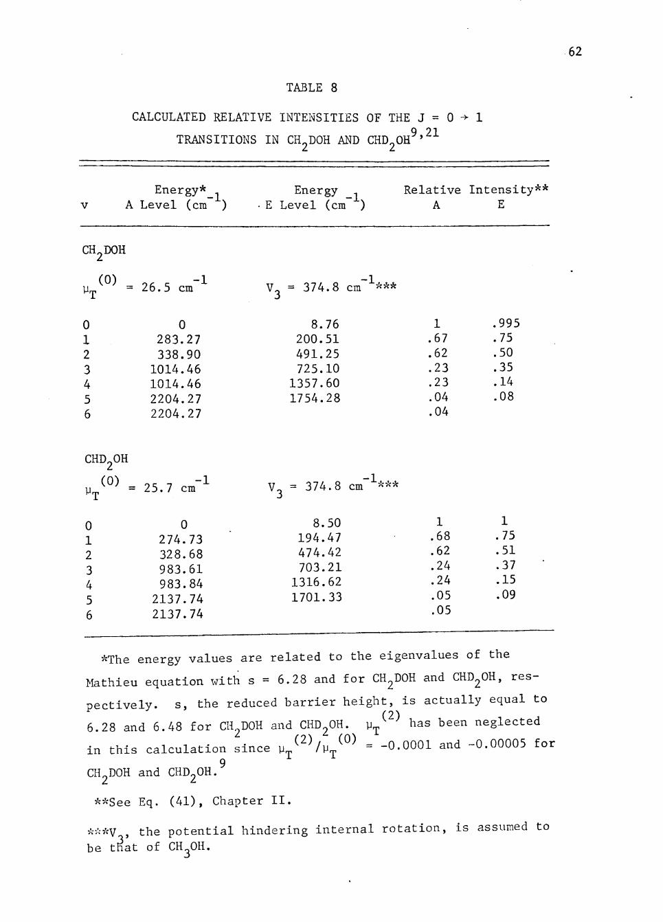
relative intensities are given in Table 7. The calculation of the rela
tive intensities is shown in Table 8. No correlation between any two
different molecules should be attempted since no effort was made to
reproduce the power density and number of absorbing molecules in the
cell. The assignments for the J = 0 1 transition are given in Table 5.
In Chapter II the total splittings of the J = 0 -> 1, n = 0 transi
tions were calculated to be 70.84 and 70.00 MHz compared to the measured
splitting of 86.86 and 103.28 MHz for CH DOH and CHD^OH respectively.

TABLE 7
RELATIVE INTENSITIES OF THE J = 0 -> 1 LINES IN CH DOH AND CHD OH
•
Line
CH DOH
44713.86 44651.59 44627.00
44582.19 44558.87
44512.59 44511.86
44495.86 44456.47
CHD2OH
41669.42 41653.83 41566.14
41557.18 41533.60
41491.29 41488.09
41474.15 41442.29
Observed Intensity
1 1. 1
.47
.43
.28
.28
.07
.07
1 .97
1
.37
.40
.27
.27
.07
.07
Calculated Intensity
1 1 1
.75
.67
.62
.50
.23
.35
1 1 1
.75
.68
' " .62 .51
.24
.37
62
TABLE 8
CALCULATED RELATIVE INTENSITIES OF THE J = 0 1
TRANSITIONS IN CH DOH AND CHD OH ' -'"
Energy*_. Energy _ Relative Intensity** A Level (cm ) • E Level (cm ) A E
CH
y^
0 1 2 3 4 5 6
2D0H
(0) 26.5 cm
0 283. 338. 1014. 1014. 2204. 2204.
,27 ,90 ,46 .46 .27 .27
V3 = 37^
8. 200. 491. 725.
1357. 1754.
h.8 cm ***
76 51 25 10 ,60 ,28
1 .67 .62 .23 .23 .04 .04
.995
.75
.50
.35
.14
.08
CHD OH
(0) _ yrj.
0 1 2 3 4 5 6
25.7 cm
C 274. 328. 983. 983.
2137. 2137.
)
73 68 ,61 ,84 ,74 ,74
v., = 374.8 cm """***
8.50 1 1 194.47 .68 .75 474.42 .62 .51 703.21 .24 .37 1316.62 .24 .15 1701.33 .05 .09
.05
*The energy values are related to the eigenvalues of the
Mathieu equation with s = 6.28 and for CH^DOH and CHD^OH, res
pectively, s, the reduced barrier height, is actually equal to (2)
6.28 and 6.48 for CH^DOH and CHD^OH. y^' has been neglected
in this calculation since y^^Vy^^°^ = "0.0001 and -0.00005 for
9 CH DOH and CHD2OH.
**See Eq. (41), Chapter II.
:-•>vv , the potential hindering internal rotation, is assumed to
be t^at of CH^OH.

63
This discrepancy arises mainly from the neglection of the dynamic
interaction between internal and overall rotation and to a lesser degree
the neglection of the interaction between vibration and rotation. Not
only do these interactions increase the total splitting, they also push
two of the torsional substates apart giving the three unequally spaced
lines observed rather than equally spaced as calculated.
The calculated splittings indicate that the a-dependence of the
rotational constants in the two molecules is nearly identical. Com
paring the measured splitting, it can be deduced that the dynamic
interaction is larger for the doubly deuterated molecule than for the
singly deuterated. This probably is due to the greater angle between
the internal rotation axis and the principle axis of the molecule in
CHD OH. -"-
A rigorous calculation to determine the rotational constants for
the various configurations of CH DOH and CHD^OH should be finished in
the near future at which time a comparison between the theoretical and
experimental results should provide the equilibrium orientation of the
methyl alcohol molecule.

LIST OF REFERENCES
1. W. Gordy, W. V. Smith, and R. F. Trambarulo, Microwave Spectroscopy (Dover Publications, Inc., New York, 1966), p. 2.
2. P. Venkateswarlu, H. D. Edwards, and W. Gordy, J. Chem. Phys. 23. 1195 (1955). —
3. P. Venkateswarlu and W. Gordy, J. Chem. Phys. , 1200 (1955).
4. E. V. Ivash and D. M. Dennison, J. Chem. Phys. , 1804 (1953).
5. D. G. Burkhard and D. M. Dennison, Phys. Rev. , 408 (1951).
6. R. H. Hughes, W. E. Good, and D. K. Coles, Phys. Rev. 8^, 418 (1951)
7. C. R. Quade and C. C. Lin, J. Chem. Phys. 8, 540 (1963).
8. J. V. Knopp, Master's Thesis, University of Delaware (1965).
9. J. V. Knopp and C. R. Quade, J. Chem. Phys. , 3317 (1968).
10. E. V. Condon and G. H. Shortley, The Theory of Atomic Spectra
(Cambridge at the University Press, New York, 1964), pp. 45-50.
11. Reference 9.
12. Reference 9.
13. C. H. Townes and A. L. Schawlow, Microwave"Spectroscopy (McGraw-
Hill Book Co., Inc., New York, 1955), pp. 248-251.
14. Reference 1.
15. Reference 1.
16. L. Pauling and E. B. Wilson, Jr., Introduction to Quantum Mechanics (McGraw-Hill Book Co., Inc., New York, 1935), Chapter XI.
17. K. B. McAffe, Jr., R. H. Hughes, and E. B. Wilson, Jr., Rev. Sci. Instr. , 821 (1949).
18. L. N. Ridenour, Editor-in-Chief, MIT Radiation Laboratory Series (McGraw-Hill Book Co., Inc., New York, 1948-50), Vols. 8, 10, 15, 17.
19. L. C. Hedrick, Rev. Sci. Instr. 2^, 781 (1949).
20. A. S. Esbitt and E. B. Wilson, Jr., Rev. Sci. Instr. _34, 901 (1963).
64

65
21. C. C. Lin and J. D. Swalen, Rev. Mod. Phys. , 841 (1959).
22. Reference 3.
23. P. Kisliuk and C. H. Townes, Molecular Microwave Spectra Tables (U. S. Government Printing Office, Washington, 1952), p. 84
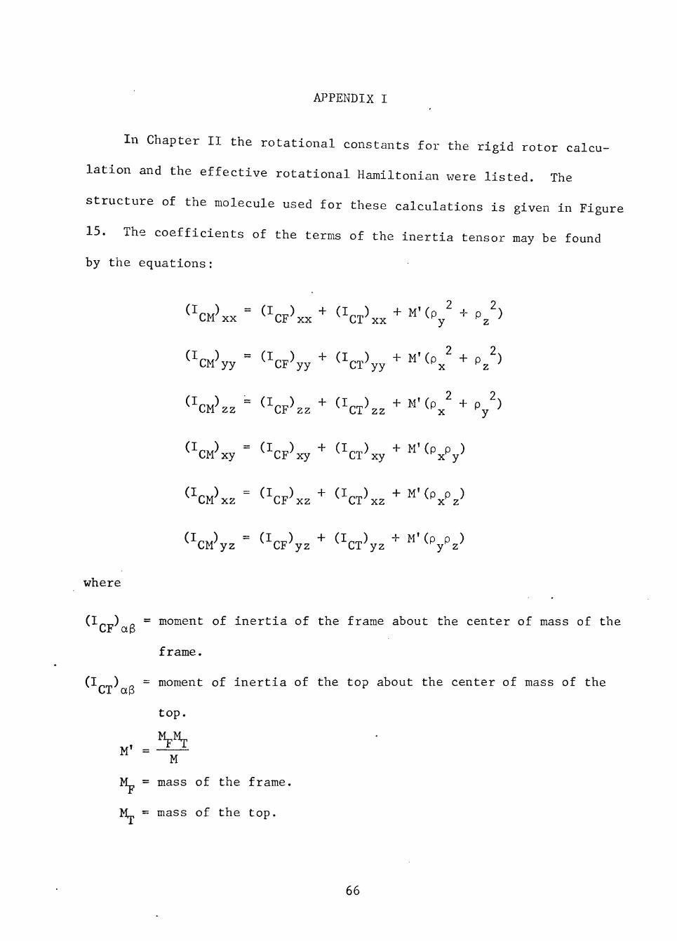
APPENDIX I
In Chapter II the rotational constants for the rigid rotor calcu
lation and the effective rotational Hamiltonian x ere listed. The
structure of the molecule used for these calculations is given in Figure
15. The coefficients of the terms of the inertia tensor may be found
by the equations:
" c M > x x = ( W x x + ( V x x + « ' ( P y ' + Pz '^
< V y y = " c F > y y + " c T > y y + « ' < P x ' + p / )
"CM zz CF zz ^ CT zz X y
(Wxy= ( V x y + ( CT)xy + ^'(PxV
( V x z = ( V x z + ( V x z + ^ ' V z ^
(Wyz= "cF>yz+ <Vyz + " ' V ^ ^
where
(I^^) ^ = moment of inertia of the frame about the center of mass of the CF ap
f rame.
(I^^) ^ = moment of inertia of the top about the center of mass of the CT ap
top.
M
M^ = mass of the frame.
'M = mass of the top.
66
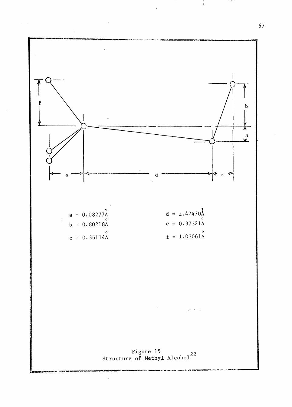
67
%. - r < -iitr^raTXiiM ^ - -> ^(^ C
= 0.08277A o
= 0.80218A
d = 1.42470A o
e = 0.37321A
c = 0.36114A f = 1.03061A
Figure 15 Structure of Methyl Alcohol
22
Ifc-flLaraaeur^f^t^*^ niHW •III! • • • • • I III •

68
M = mass of the molecule.
p^ - components of a vector from the center of mass of the frame to
the center of mass of the top.

APPENDIX II
The accuracy of the frequency measurements made in this thesis v:as
determined by measuring the frequency of twelve lines of the ammonia
spectrum and the J = 0 -> 1 transitions in CH OH. The measured frequency
of the ammonia lines along with the accepted frequency and the error are
tabulated in this Appendix. The frequencies measured for the CH OH
lines are given in Table 4.
FREQUENCY CALIBRATION BY A>IMONIA
Rotational Stat
J
3 7 2 8 9 1 2 3 4 10 5 6
e
K
2 6 1 7 8 1 2 3 4 9 5 6
Measured Frequency
MHz
21834.11 21924.90 23098.79 23232.20 23657.46 23694.49 23722.61 23870.14 24139.40 24205.29 24532.94 25056.05
Accepted „„ Frequency
MHz
21834.10 22924.91 23098.78 23232.20 23657.46 23694.48 23722.61 23870.11 24139.39 24205.25 24532.94 25056.04
Error
MHz
+0.01 -0.01 +0.01 0.00
+0.01 +0.02 0.00
+0.03 +0.01 +0.04 0.00
+0.01
69
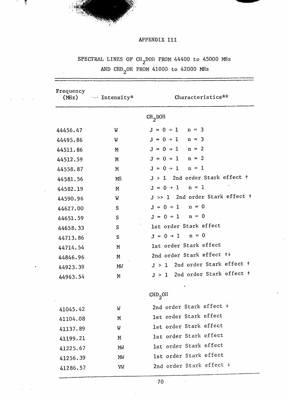
APPENDIX III
SPECTRAL LINES OF CH DOH FROM 44400 to 45000 MHz
AND CHD OH FROM 41000 to 42000 MHz
Frequency (MHz)
44456.47
44495.86
44511.86
44512.59
44558.87
44581.56
44582.19
44590.96
44627.00
44651.59
44658.33
44713.86
44714.54
44846.96
44923.39
44963.54
41045.42
41104.08
41137.89
41199.21
41225.67
41256.39
41286.57
-' Intensity*
W
W
M
M
M
MS
M
W
S
S
S
S
M
M
m M
w M
w M
m m vw
Characteristics**
CH^DOH
J = 0->1 n = 3
J = 0->1 n = 3
J = 0->1 n = 2
J = 0 ^ 1 n = 2
J = 0->1 n = l
J > 1 2nd order Stark effect i
J = 0 -> 1 n = 1
J >> 1 2nd order Stark effect ^
J = 0->1 n = 0
J = 0->1 n = 0
1st order Stark effect
J = 0->1 n = 0
1st order Stark effect
2nd order Stark effect i^
J > 1 2nd order Stark effect f
J > 1 2nd order Stark effect f
CHD2OH
2nd order Stark effect +
1st order Stark effect
1st order Stark effect
1st order Stark effect
1st order Stark effect
1st order Stark effect
2nd order Stark effect 1
70
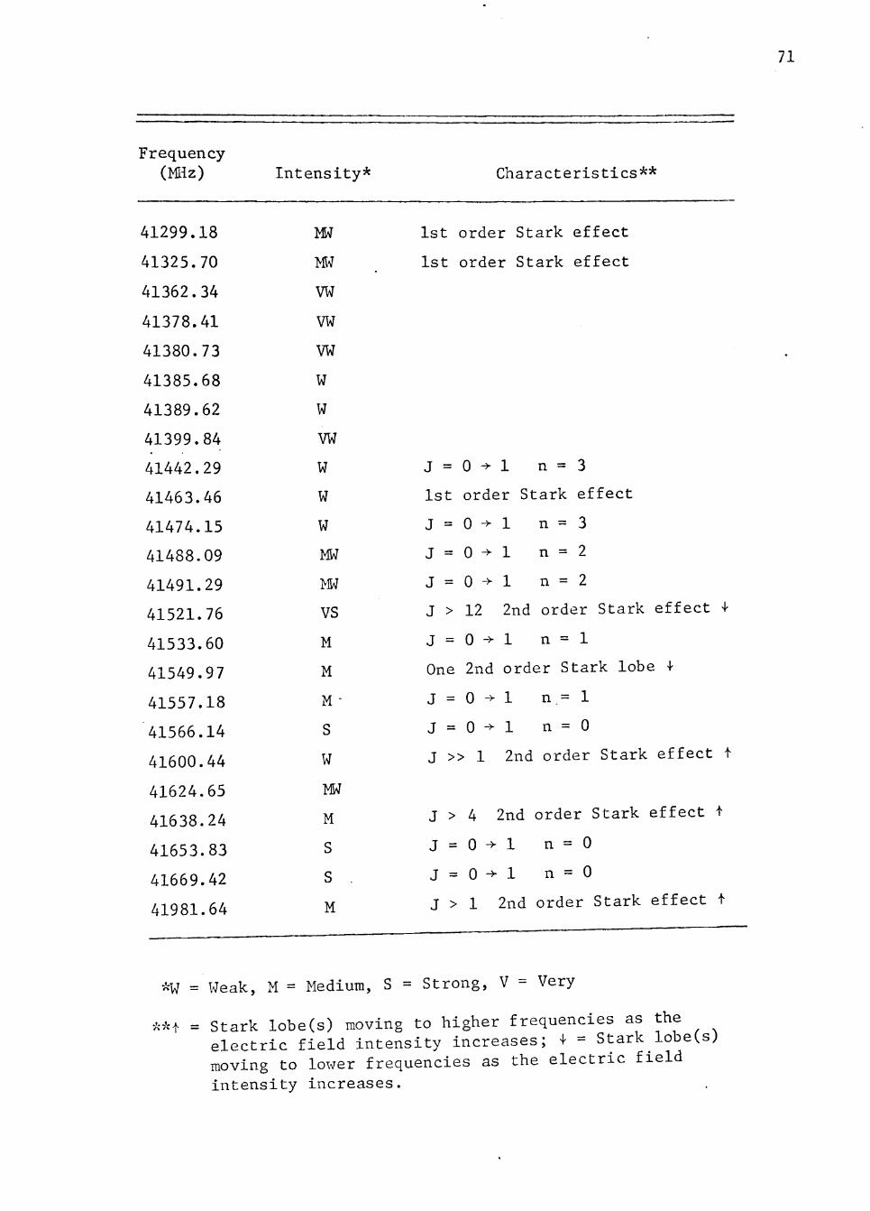
71
Frequency (MHz) Intensity* Characteristics**
41299.18
41325.70
41362.34
41378.41
41380.73
41385.68
41389.62
41399.84
41442.29
41463.46
41474.15
41488.09
41491.29
41521.76
41533.60
41549.97
41557.18
41566.14
41600.44
41624.65
41638.24
41653.83
41669.42
41981.64
MW
ME
VW
VW
VW
W
W
VW
W
W
W
MW
MW
vs
M
M
M •
S
w
MW
M
S
s
M
1st order Stark effect
1st order Stark effect
J = 0-^1 n = 3
1st order Stark effect
J = 0->1 n = 3
J = 0 ^ 1 n = 2
J = 0 ^ 1 n = 2
J > 12 2nd order Stark effect +
J = 0->1 n = l
One 2nd order Stark lobe l-
J = 0 ^ 1 n.= 1
J = 0->1 n = 0
J >> 1 2nd order Stark effect f
J > 4 2nd order Stark effect t
J = 0->1 n = 0
J = 0->1 n = 0
J > 1 2nd order Stark effect i
*W = Weak, M = Medium, S = Strong, V = Very
:-*f = Stark lobe(s) moving to higher frequencies as the electric field intensity increases; -I- = Stark lobe(s; moving to lower frequencies as the electric field intensity increases.