Embed Size (px)
Citation preview
The influence of polymer concentration and chainarchitecture on free surface displacement flows
of polymeric fluids
Gandharv Bhatara
Department of Chemical Engineering, Stanford University, Stanford,California 94305
Eric S. G. Shaqfeh
Departments of Chemical and Mechanical Engineering, Stanford University,Stanford, California 94305
Bamin Khomamia)
Materials Research Laboratory, Department of Chemical Engineering, WashingtonUniversity, St. Louis, Missouri 63130
(Received 19 October 2004; final revision received 16 June 2005�
Synopsis
We examine the effect of polymer concentration and chain architecture on the steady statedisplacement of polymeric fluids by air in between two infinitely long closely spaced parallelplates, i.e., Hele-Shaw flow. A stabilized finite element method coupled with a pseudosolid domainmapping technique is used for carrying out the computations. The constitutive equations employedin this study are the Finitely Extensible Nonlinear Elastic–Chilcott Rallison �FENE-CR� and theFinitely Extensible Nonlinear Elastic–Peterlin �FENE-P� models for dilute solutions, the Giesekusconstitutive equation for dilute, semidilute and concentrated solutions, and the Extended Pom-Pom�XPP� constitutive equation for linear and branched polymeric melts. Our study indicates thepresence of a recirculation flow at low Ca and a bypass flow at high Ca irrespective of polymerconcentration and chain architecture. We show that the interfacial dynamics in both therecirculation and the by-pass flow depend on extensional hardening and shear thinningcharacteristics of the fluids. In the recirculation flow, we observe the formation of normal elasticstress boundary layers in the capillary transition region, an accompanying increase in thefilm thickness and a compression of the bubble in the capillary transition region, at moderate Wi.In the bypass flow, in addition to the elastic stress boundary layer in the capillary transitionregion, an additional stress boundary layer is observed at the tip of the bubble. The amount offilm thickening, the magnitude of the stress in the stress boundary layer and the amount of bubblecompression are largest for the most extensional hardening fluids and reduce with decreasingextensional hardening and increasing shear thinning. We show that the film thickness is determinedby two competing forces, i.e., normal stress gradients in the flow direction, in the capillarytransition region �recirculation flow� and the tip region �bypass flow� and shear stress gradients
a�Author to whom correspondence should be addressed; electronic mail: [email protected]; FAX �314 935
7211© 2005 by The Society of Rheology, Inc.929J. Rheol. 49�5�, 929-962 September/October �2005� 0148-6055/2005/49�5�/929/34/$25.00
930 BHATARA, SHAQFEH, AND KHOMAMI
in the gap direction. For both the recirculation and the bypass flow, we show how the filmthickness scales with fluid normal stresses and shear viscosities, and develop correlations forthe film thickness as a function of Ca and Wi. © 2005 The Society of Rheology.�DOI: 10.1122/1.2000969�
I. INTRODUCTION
The displacement of Newtonian and viscoelastic fluids by air in long narrow tubesplays a central role in many industrial applications such as polymer processing, coatingtechnology, gas-assisted injection molding and enhanced oil recovery �Taylor �1961�,Cox �1962�, Bretherton �1961�, Bonn et al. �1995�, Ruschak �1985�, Coyle et al. �1990�,Poslinski et al. �1995��. Consequently, numerous researchers have focused their attentionon Newtonian displacement flows in a variety of geometries to better understand theinterfacial dynamics of free surface flows and prevent free surface instabilities that occurin this class of flows �Pearson �1960�, Pitts and Greiller �1961�, Sullivan and Middleman�1979�, Coyle et al. �1990�, Rabaud et al. �1990��. However, the number of studiesdealing with viscoelastic fluids is very limited �Shaqfeh �1995�, Ruschak �1985�, Larson�1992��. To date, most studies have been concerned with film thickness measurements�thickness of the film formed when the fluid is displaced by air� since in most industrialapplications, control and uniformity of the film thickness is of primary importance.Hence, our primary focus in this paper will be on examining the influence of polymerconcentration and chain architecture on film thickness in a model free surface displace-ment flow.
In case of Newtonian fluids, the first experimental studies were carried out by Taylor�1961� and Cox �1962� who measured the film thickness as a function of Ca �where Cais the Capillary number, defined as the ratio of viscous forces to surface tension� obtainedwhen a viscous fluid is displaced out of a tube by an air bubble. The thickness of the filmleft on the walls by the displaced fluid was observed to increase with increasing Ca.Bretherton �1961� conducted an asymptotic analysis, in addition to experiments, andfound good agreement between his asymptotic theory and the experimentally measuredfilm thickness at vanishingly small Ca. Reinelt and Saffman �1985� obtained film thick-ness results using a finite difference scheme and observed a film thickening effect withincreasing Ca. More recently, Park and Homsy �1984� have developed a theory describ-ing two-phase displacement in the gap between closely spaced planes under the assump-tions of small Ca and ratio of gap width to transverse characteristic length, and subse-quently showed that the film thickness scales as Ca1/3.
Turning to the literature on viscoelastic fluids, we find a scarcity of literature in bothcomputational and experimental aspects of the problem. Bonn et al. �1995� using solu-tions of polyethylene oxide �PEO� reported an increase in the film thickness over thatfound for Newtonian fluids. Linder et al. �2002� carried out experiments in a Hele-Shawcell geometry and observed a film thickness increase over that found for Newtonian fluidsusing PEO, and a film thickness decrease using xanthane. They attributed the film thick-ening effect for PEO to the high elongational viscosity and large normal stresses thatPEO exhibits, although no clear correlations were developed with Wi. Huzyak et al.�1997� reported strong film thickening effects using highly elastic, nonshear thinning,polyisobutene-polybutene �PIB-PB� based Boger fluids. Lee et al. �2005� in an experi-mental study, of a free surface displacement flow of PIB-PB Boger fluids under gravitystabilization in an eccentric cylinder geometry, found significant film thickening due topresence of elasticity. The first theoretical study of a free surface displacement flow of aviscoelastic fluid was carried out by Ro and Homsy �1995�. Specifically, the authors
1/3 1/3
formulated a double perturbation expansion in powers of Ca and Wi /Ca , �where Wi
931FREE SURFACE DISPLACEMENT FLOWS
is the Weissenberg number, and it provides a measure of the elasticity of the flow throughthe relaxation time of the polymer� and concluded that for small values of Wi /Ca1/3, thefluid elasticity induces resistance to streamwise straining and hence reduces the filmthickness. However, this theory is valid for small values of Ca and Wi.
Besides the aforementioned experimental and theoretical contributions, numericalstudies have been performed by Pasquali and Scriven �2002�, Lee et al. �2002�, andBhatara et al. �2004�, on the steady-state displacement of viscoelastic fluids by an airbubble. Specifically, Pasquali and Scriven �2002� examined the flow dynamics of airdisplacing fluid for a slot coating flow using dilute and semidilute polymer solutions.They observed the formation of layers of molecular stretch under the free surface down-stream of the stagnation point, in the capillary transition region. Furthermore, theyshowed that the layers of molecular stretch are largest for the extensible and semiexten-sible molecules and effectively smaller for more rigid molecules. Lee et al. �2002�,examined both the Hele-Shaw cell geometry and the slot coating geometry for dilutepolymer solutions using the Oldroyd-B, FENE-CR and FENE-P constitutive equations. Inthe Capillary number regime considered in their study �i.e., Ca�1.0�, the flow is char-acterized by a recirculation pattern and the authors show the formation of elastic normalstress boundary layers in the capillary transition region at moderate values of Wi. Fur-thermore, the authors observed that the formation of these stress boundary layers gener-ates a strong positive normal stress gradient in the flow direction of the capillary transi-tion region that results in film thickening. In addition, it is suggested that the formation ofthese stress boundary layers is due to the planar extensional nature of the flow near thefree surface. Bhatara et al. �2004� extended the FENE-CR simulations to a much largerrange of Ca and Wi and also incorporated the effect of gravity and channel divergence.They identify the presence of two distinct flow regimes. In the absence of gravity, arecirculation flow at low Ca �Ca�1.0� and a bypass flow at high Ca �Ca�1.0�. In therecirculation flow, in addition to the film thickening effect, the authors observe a menis-cus invasion phenomenon when the stresses in the boundary layer become very large. Inaddition, it is also ascertained that the formation of the elastic normal stress boundarylayer is mostly a local phenomenon, largely independent of geometrical considerations.Specifically, by increasing the channel divergence the onset of the stress boundary layerand the accompanying film thickening effect is delayed to higher Wi. However, the filmthickness normalized with the maximum normal stress in the elastic stress boundary layercollapses onto a single curve.
Motivated by this fact, we have considered the effect of concentration and chainarchitecture on the flow dynamics of the air displacing fluid flow in a Hele-Shaw cellgeometry to ascertain whether the film thickness can be estimated based on specificmaterial properties and the dynamics of the localized stress boundary layers near the freesurface. More specifically, we attempt to draw correlations between film thickness andnormal stresses in the localized stress boundary layer near the free surface and therheological characteristics of the fluid model, which in turn indirectly relate to predictionsbased on concentration and chain architecture effects. To this end, we employ a variety ofconstitutive equations to model dilute and concentrated polymeric solutions as well aslinear and branched polymeric melts. For the dilute solutions we employ the FENE-CR�Chilcott and Rallison �1988�� and FENE-P �Bird et al. �1987�, Bird et al. �1980�� con-stitutive equations. To model dilute, semi-dilute and concentrated solutions we use theGiesekus constitutive equation �Bird et al. �1980�, Giesekus �1982�� and for polymericmelts we use the XPP �Verbeeten et al. �2001, 2002�� �for both linear and branched
polymers� constitutive equation. The choice of the constitutive equations has been made
932 BHATARA, SHAQFEH, AND KHOMAMI
to satisfy the primary criterion of being able to model the effect of concentration andchain architecture of polymeric fluids, while retaining sufficient mathematical simplicityfor computational tractability �i.e., continuum level description�.
II. MATHEMATICAL FORMULATION
The governing equations and the solution methodology for the steady free surfaceproblem have been presented in detail in the studies conducted by Lee et al. �2002� andBhatara et al. �2004� and we reproduce the equations briefly in this paper.
For the two-dimensional, steady free surface problem depicted in Fig. 1 the governingequations that impose conservation of mass and momentum for an incompressible fluid inthis geometry, in the absence of gravity and inertia, are
�� · u� = 0, �1�
− ��P
Ca+ �� · �= = 0, �2�
where u� is the velocity vector, P is the pressure and �= is the total stress tensor formed bythe sum of the Newtonian solvent stress, �=s, and the polymer stress, �=p. Ca is the capillarynumber and is defined as Ca=�U /�, where � is the total viscosity of the fluid at zeroshear rate, U is the characteristic velocity of the problem, and � is the surface tension.
The basic equations are nondimensionalized as
�x,y��=��b,b�, �u,v��=�U, P�=��
b, �= �=�
�U
b. �3�
A. Dilute polymeric solutions: FENE-CR and FENE-P models
As mentioned before, to model the dynamics of dilute polymeric solutions, we employelastic dumbbell models, namely, the FENE-CR �for Boger fluids� and FENE-P �to ex-amine the effect of shear thinning� models. Several studies �Lee et al. �2002�, Pasqualiand Scriven �2002�, Bhatara et al. �2004�, Grillet et al. �1999�� have previously shown theadequacy of these models to describe the interfacial dynamics of this class of fluids in avariety of simple and complex kinematics flows.
Under steady flow conditions, the constitutive equation for a FENE-CR model is given
FIG. 1. Schematic of the Hele-Shaw cell flow. The flow domain can be divided into three distinct regions: thethin film region, the capillary transition region, and the parallel flow region.
by
933FREE SURFACE DISPLACEMENT FLOWS
u� · �� C= = C= · �u=
+ �u=
T · C= −f�R�Wi
�C= − I=� , �4�
where Wi=U� /b �b is the gap separation between the plates, � is the relaxation time ofthe polymeric fluid and U is the mean fluid velocity�. I= is the identity matrix, C= is thepolymer conformation tensor and represents an ensemble average of the dyadic productRR= of the dumbell end to end vector R� . f�R� is the entropic spring force law, given by
f�R� =1
1 −Tr�C�
L2
, �5�
where L is the finite extensibility parameter, i.e., the ratio of the length of a fully extendedpolymer to its equilibrium length. The larger the value of L, the more extensible is thepolymer. The total stress is written as the sum of the viscous stress and the polymerstress,
�= = 2S�̇=
+�1 − S�
Wif�R��C= − I=� , �6�
where �̇=
is the strain rate tensor, while S is the ratio of the solvent viscosity to the totalviscosity and provides a measure of polymer concentration in the fluid. The FENE-Pmodel can be obtained by substituting the term −f�R��C= − I=� /Wi by −�f�R�C= − I=� /Wi.
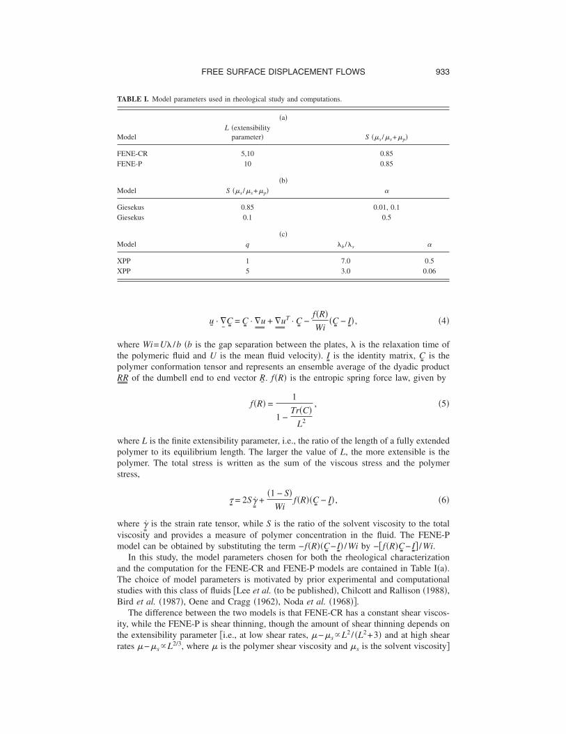
In this study, the model parameters chosen for both the rheological characterizationand the computation for the FENE-CR and FENE-P models are contained in Table I�a�.The choice of model parameters is motivated by prior experimental and computationalstudies with this class of fluids �Lee et al. �to be published�, Chilcott and Rallison �1988�,Bird et al. �1987�, Oene and Cragg �1962�, Noda et al. �1968��.
The difference between the two models is that FENE-CR has a constant shear viscos-ity, while the FENE-P is shear thinning, though the amount of shear thinning depends onthe extensibility parameter �i.e., at low shear rates, �−�sL2 / �L2+3� and at high shear
2/3
TABLE I. Model parameters used in rheological study and computations.
�a�
ModelL �extensibility
parameter� S ��s /�s+�p�
FENE-CR 5,10 0.85FENE-P 10 0.85
�b�Model S ��s /�s+�p�
Giesekus 0.85 0.01, 0.1Giesekus 0.1 0.5
�c�Model q �b /�s
XPP 1 7.0 0.5XPP 5 3.0 0.06
rates �−�sL , where � is the polymer shear viscosity and �s is the solvent viscosity�
934 BHATARA, SHAQFEH, AND KHOMAMI
�Bird et al. �1987��. In a steady shear flow, i.e., u=y, v=w=0, at a Wi of 1.0, the FENE-P�L=10� model starts to display a slight amount of shear thinning of viscosity while theFENE-CR model remains nonshear thinning. Furthermore, the first normal stress coeffi-cient, �1, shear thins for both models, while the second normal stress coefficient, �2, iszero �Bird et al. �1987��.
In a steady planar extensional flow, i.e., u=x, v=−y, w=0, both models display sig-nificant extensional hardening at Wi=0.5. Physically, this can be understood as the coilstretch transition that the polymer chains undergo at Wi=0.5. Furthermore, it can beobserved that the extensional viscosity is bounded as Wi approaches infinity �asymptotesto L2 for both FENE-CR and FENE-P�. In transient planar extensional flow, bothFENE-CR �L=10� and FENE-CR �L=5� display extensional viscosities which increasemonotonically with increasing strain, with no stress overshoot, and tending asymptoti-cally towards values corresponding to steady planar extensional flow.
It is worth noting that we are interested in the planar extensional viscometric behaviorrather than the uniaxial extensional behavior because the flow �of the air displacing fluidin the Hele-Shaw cell� at the free surface is planar extensional, and we subsequentlyrelate the normal stresses generated at the free surface to the extensional viscosity of thevarious models.
B. Dilute, semidilute and concentrated solutions: Giesekus model
The Giesekus model �i.e., an elastic dumbbell model with anisotropic hydrodynamicdrag on the beads� has been selected for modeling the dynamics of semidilute and con-centrated polymeric solutions due to the fact that prior studies have shown that it canadequately describe dynamics of this class of flows in both simple and complex kinemat-ics flows �Giesekus �1982�, Burghardt et al. �1999��. Under steady flow conditions theconstitutive equation for the Giesekus model can be written as
u� · �� C= = C= · �u=
+ �u=
T · C= − � f�R�Wi
C= − I=� +
Wi�C= − I=��f�R�C= − I=� . �7�
The parameter is a model parameter and the term containing is attributed toanisotropic hydrodynamic drag on the constituent polymer molecules. It should be notedthat can be indirectly related to the concentration of the polymer, i.e., =0 representsdilute solutions, while =0.5 represents concentrated solutions. For physically relevantresults it is required that 0��0.5, as for values of �0.5, the shear stress ��xy� plottedas a function of Wi displays a maximum, which is not observed experimentally for thisclass of fluids �Bird et al. �1987��. The model parameters chosen for this study arecontained in Table I�b�.
Under steady shear flow the Giesekus model displays shear thinning. The decrease inthe shear viscosity with Wi is enhanced as is increased. In steady shear flow �i.e., u=x, v=w=0�, for �0, it can be shown that the shear viscosity asymptotes to ��1−� /at high shear rates �Bird et al. �1987��. The first normal stress coefficient decreases withincreasing shear rate and the rate of decline increases with increasing . The secondnormal stress coefficient is nonzero and negative, and can be varied in magnitude relativeto the first normal stress coefficient by adjusting the value of . Under steady planarextensional flow, for low values of , extensional hardening �with finite asymptoticvalue� is observed. The magnitude of the extensional viscosity decreases with increasing. At =0.5, the Giesekus model displays a very slight extensional hardening behavior
and the steady extensional viscosity is largely independent of strain rate. Under transient
935FREE SURFACE DISPLACEMENT FLOWS
planar extensional flow, for all values of ��, the extensional viscosity shows a monotonicincrease with increasing strain and no stress overshoot.
C. Polymeric melts: XPP model
Since theories based on the concept of reptation proposed by deGennes �Doi andEdwards �1986�, deGennes �1971�� have emerged as the primary tool for describing therheology of entangled polymeric systems, we have selected the pom-pom constitutiveequation �Verbeeten et al. �2001, 2002�, Milner and Mcleish �1998�� to investigate thedynamics of polymeric melts. This choice has been motivated by the fact that this modelnot only contains the essential physics to describe the dynamics of entangled polymericsystems �i.e., evolution equations for the orientation and stretch�, but also, by appropriateselection of the model parameters, one can describe the nonlinear rheology of both linearand branched entangled polymeric fluids.
The key feature of the model is the decoupling of relaxation times for stretch andorientation. The simplified topology consists of a chain backbone and a number of dan-gling arms on both ends of the backbone. Verbeeten et al. �2001� incorporated localbranch-point displacement and modified the orientation equation of the original differen-tial version to the extended Pom-Pom model in order to resolve three major issues:discontinuities in steady state elongation, unbounded orientation at high strain rates, anda zero second normal stress difference in shear. In addition the XPP model can be writtenin a differential form that makes it computationally attractive. The constitutive behaviorof a single mode XPP model can be represented with the following equations,
u� · �� �= − �u=
T · �= − �= · �u=
+ ����−1 · �= = 2GD= , �8�
where G is the plateau modulus and D= = �1/2���u=
+�u=
T� is the rate of deformation tensor.The function ���=�−1 is defined as
���=�−1 =1
�b�
G�= + F��=�I= + G„F��=� − 1…�=−1� , �9�
with
F��=� = 2re���−1��1 −1
�� +
1
�2�1 − Tr��= · �=�
3G2 � , �10�
and
� =�1 +Tr��=�3G
, �11�
r =�b
�s, �12�
=2
q, �13�
where � is the backbone tube stretch, defined as the length of the backbone tube dividedby the length at equilibrium, I= is the unit tensor, �b is the relaxation time of the backbonetube orientation �equal to the linear relaxation time�, �s is the relaxation time for thestretch, a parameter defining the amount of isotropy, a parameter signifying the
influence of the surrounding polymer chains on backbone tube stretch, and q represents
936 BHATARA, SHAQFEH, AND KHOMAMI
the number of arms at the ends of the backbone. For this study, we use two values of q,i.e., q=1 to represent linear melts, and q=5 to represent branched melts. The value ofq=5 is chosen so as to attain extensional thickening behavior typical of branched poly-meric melts, while ensuring that the model produces monotonic shear stress as a functionof Wi. The model parameters used in this study are contained in Table I�c�.
It is worth noting that using the aforementioned definition of backbone stretch �see Eq.�15��, the computations stop if Tr��=� /3G�−1, which is aphysical since Tr��=� should bepositive. This has been shown to occur before at the front and back stagnation points inthe flow around a cylinder at sufficiently high Wi �Verbeeten et al. �2002��. This problemcan be obviated by rewriting the backbone stretch equation as a double-equation XPPmodel and in this paper we implement the XPP model in an equivalent double-equationfashion, i.e., we express the polymeric stress explicitly in terms of the backbone stretch��� and the orientation tensor �Q
=� as
�= = 3G�2Q=
− GI= . �14�
The evolution equations for the orientation tensor and the backbone tube stretch are givenby
u� · �� Q=
− �u=
T · Q=
− Q=
· �u=
+ 2�D= :Q=
�Q=
+1
�b�2�3�4Q=
· Q=
+ �1 − − 3�4 Tr�Q=
· Q=
��Q=
−1 −
3I=� = 0, �15�
�̇ = ��D= :Q=
� −
exp2
q�� − 1�
�s�� − 1� . �16�
Under shear flow, the XPP model, like the FENE-P and Giesekus model, displaysshear thinning behavior. The first normal stress coefficient decreases at higher shear rates,while the second normal stress coefficient is nonzero and negative. In steady extensionalflow, however, unlike the FENE-CR, FENE-P and Giesekus models, XPP �q=5� displaysa region of extensional hardening, followed by a region of mild extensional thinning. Thisbehavior is typical of branched polymeric melts �Verbeeten et al. �2001, 2002��. Settingq=1 results in a very small amount of extensional hardening and hence the XPP modelwith q=1 can be used to model the behavior of linear entangled polymeric systems.Under transient planar extensional flow, the XPP model displays a monotonic increase inthe extensional viscosity with increasing strain for both q=1 and q=5. It is also worthnoting, that for values of greater than zero, the steady shear and transient and steadyplanar extensional behavior is independent of the value of .
D. Boundary conditions
The free surface boundary conditions are the kinematic condition
u� · n� = 0, �17�
the normal stress balance
n� · ��= − I=P� =�� s · n�
Ca, �18�
and the vanishing shear stress
937FREE SURFACE DISPLACEMENT FLOWS
n� · �= · t� = 0, �19�
where n� and t� are the unit vectors normal and tangent to the free surface respectively and�� s denotes the surface divergence operator. The governing equations are solved by con-sidering a coordinate system that moves at the same speed as the bubble tip. In thisreference frame the corresponding boundary conditions are the no slip condition on thesolid wall,
u = 1, v = 0; y = 0, 0 � x � � , �20�
symmetry conditions at the centerline,
�sy = 0, v = 0; y =1
2, 0 � x � xc �21�
xc, u� = 0, �22�
where xc refers to the x coordinate of the bubble tip. At the outflow, a fully developedvelocity profile is assumed in the thin film, i.e.,
�2u
�y2 = 0, �23�
while far from the air fluid interface the velocity profile takes on the following form forthe FENE-CR model �Lee et al. �2005�, Reinelt and Saffman �1985��:
u = 6„1 − 2h��1 − �h��2�…y�y − 1� + 1, v = 0. �24�
The quantity h� is the dimensional thickness of the hydrodynamic coating left behind bythe advancing air bubble, and its value is determined as part of the solution. For the restof the models �FENE-P, Giesekus, XPP� the velocity profiles are dictated by nonlineardifferential equations that are solved numerically. Specifically, at the inflow, a unidirec-tional shear flow �u=F�y�� is assumed and for each model the conformation tensors areevaluated using the corresponding constitutive equations �Giesekus �1982�, Bhatara et al.�2004�; Sureshkumar et al. �1997�, Lee et al. �2002�, Arora et al. �2004�� �see AppendixA for details�.
All the boundary conditions specified above are essential boundary conditions, i.e.,they replace the respective governing equations at the boundary nodes, with the exceptionof n� ·�= ·n� which is imposed naturally.
E. Coupled DEVSS finite element–pseudosolid formulation
The stabilized FEM formulation used in this study is the scheme employed previouslyby us �Lee et al. �2002�, Bhatara et al. �2004�� and we present a brief account of it here.The DEVSS formulation proposed by Guenette and Fortin �1995�, Yurun et al. �1995�,Szady et al. �1995�, Talwar and Khomami �1992� is used to discretize the fluid governingequations. A standard Galerkin formulation is used to discretize the momentum andcontinuity equations. The streamline upwind Petrov-Galerkin method �SUPG� proposedby Brooks and Hughes �1982� is used to integrate the constitutive equations. The FEMformulation is coupled to the pseudo-solid domain mapping technique developed bySackinger et al. �1996� and Cairncross et al. �2000��. The mesh is treated as a fictitious
elastic solid, which deforms in response to boundary loads. As the mesh boundary con-
938 BHATARA, SHAQFEH, AND KHOMAMI
forms to the domain occupied by the fluid, the mesh interior moves as though it were acompressible elastic solid, and the boundary conditions relate the actual free surfaceproblem to the pseudosolid formulation.
The residual equations obtained via the FEM formulation �Lee et al. �2002�, Bhataraet al. �2004�� are solved via the Newton’s iteration method, with first order continuationin both Ca and Wi. In this study, we employ the finest mesh used in our previous studiesfor the FENE-CR model, for which it was shown to be sufficiently refined �Bhatara et al.�2004��. Since introducing shear thinning or reducing extensional thickening results inreduced stresses in the stress boundary layer in the capillary transition region as well asthe tip of the bubble, we expect the chosen discretization to perform extremely well �i.e.,produce converged results� for the remaining constitutive models considered.
III. FLOW FIELD COMPARISONS
A. Newtonian flow field
In the Newtonian flow, as the Ca is increased, the film thickness is also increased �Leeet al. �2002�, Bhatara et al. �2004��. The monotonic increase of the film thickness with Caoccurs because as the Ca is enhanced, the viscous drag on the fluid increases and propelsmore fluid into the thin film region �Ro and Homsy �1995�, Lee et al. �2002�, Bhatara etal. �2004��. As the Ca is increased the recirculation region disappears and we obtain acomplete bypass flow. The transition from the recirculation flow to the bypass flowoccurs at a Ca of about 0.85. To further quantify the flow field we calculate the effectivestrain or the second invariant of the strain rate tensor �W� and the extensional rate �E�,defined as
W =1
2�eijeij − ekk
2 � , �25�
E =�eijeji�1/2
�eijeji�1/2 + ���ij� ji�1/2�, �26�
where eij is the strain tensor and �ij is the vorticity tensor.As Ca is increased, the maximum effective strain rate �that occurs at the wall below
the thin film� is reduced. This is attributed to the increase in the hydrodynamic filmthickness with increasing Ca.
B. Viscoelastic flow field
Figure 2 illustrates the effect of elasticity on the flow field for a variety of fluids atdifferent Ca. At low Ca, for all fluids �FENE-CR, FENE-P, Giesekus and XPP�, there isa recirculation region, as observed in the Newtonian flow �see Figs. 2�a� and 2�c��.However, for the same Ca, the effect of addition of elasticity or increasing the Wi is adecrease in the strength of the recirculation region and drawing of the lateral stagnationlines towards the vertex of the bubble �Lee et al. �2002�, Bhatara et al. �2004��. At Ca oforder unity, the recirculation region disappears and a complete bypass flow is obtained�see Figs. 2�e� and 2�g��.
For both recirculation and bypass flow, the maximum effective strain rate for vis-coelastic flow is a function of the deviation in the film thickness from the Newtoniancase. As in the Newtonian flow, the maximum strain rate is observed at the wall in thethin film region �see Figs. 2�b�, 2�d�, 2�f�, and 2�h��. High strain rates are also observed
close to the interface in the capillary transition region. The latter region is of more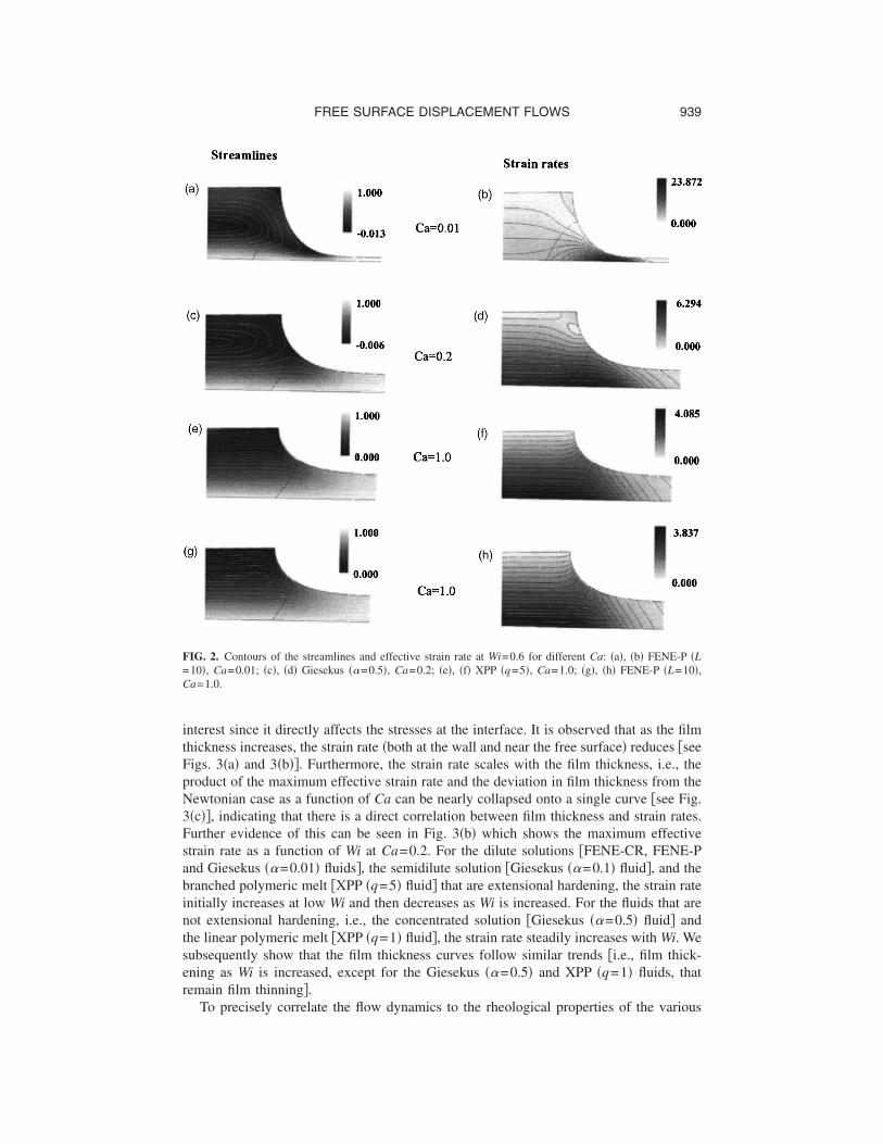
939FREE SURFACE DISPLACEMENT FLOWS
interest since it directly affects the stresses at the interface. It is observed that as the filmthickness increases, the strain rate �both at the wall and near the free surface� reduces �seeFigs. 3�a� and 3�b��. Furthermore, the strain rate scales with the film thickness, i.e., theproduct of the maximum effective strain rate and the deviation in film thickness from theNewtonian case as a function of Ca can be nearly collapsed onto a single curve �see Fig.3�c��, indicating that there is a direct correlation between film thickness and strain rates.Further evidence of this can be seen in Fig. 3�b� which shows the maximum effectivestrain rate as a function of Wi at Ca=0.2. For the dilute solutions �FENE-CR, FENE-Pand Giesekus �=0.01� fluids�, the semidilute solution �Giesekus �=0.1� fluid�, and thebranched polymeric melt �XPP �q=5� fluid� that are extensional hardening, the strain rateinitially increases at low Wi and then decreases as Wi is increased. For the fluids that arenot extensional hardening, i.e., the concentrated solution �Giesekus �=0.5� fluid� andthe linear polymeric melt �XPP �q=1� fluid�, the strain rate steadily increases with Wi. Wesubsequently show that the film thickness curves follow similar trends �i.e., film thick-ening as Wi is increased, except for the Giesekus �=0.5� and XPP �q=1� fluids, thatremain film thinning�.
FIG. 2. Contours of the streamlines and effective strain rate at Wi=0.6 for different Ca: �a�, �b� FENE-P �L=10�, Ca=0.01; �c�, �d� Giesekus �=0.5�, Ca=0.2; �e�, �f� XPP �q=5�, Ca=1.0; �g�, �h� FENE-P �L=10�,Ca=1.0.
To precisely correlate the flow dynamics to the rheological properties of the various

940 BHATARA, SHAQFEH, AND KHOMAMI
fluids, we analyze the two flow regimes separately, starting with the recirculation flowand then proceeding to the bypass flow, with particular emphasis on the recirculation flowas it is most often encountered under a variety of processing conditions �Lee et al. �2002�,Bhatara et al. �2004�, Giavedoni et al. �1997��.
IV. FILM THICKNESS AND INTERFACE DYNAMICS
A. Recirculation flow
Ro and Homsy �1995�, by employing a low Wi asymptotic analysis of the Oldroyd-Bmodel, have shown that at low Ca, the presence of elasticity will result in a small filmthinning effect. To understand the mechanism of film thinning, we briefly elucidate themechanism proposed by Ro and Homsy. The authors found that film thickness is deter-mined by two major competing forces, normal stress gradients in the flow direction �i.e.,��xx /�x�, and shear stress gradients �i.e., ��xy /�y� in the gap direction. If the normal stressgradients are positive, they would act to assist the passage of fluid elements into the thinfilm region and result in film thickening. The shear stress gradients are the viscousstresses responsible for dragging the fluid elements in the direction of the wall velocityand hence forming the hydrodynamic coating �see Fig. 4�. In the limit of small Ca andWi, the authors show that film thinning results due to the presence of negative normalstresses in the flow direction, i.e., ��xx /�x�0, that are greater than the shear stressgradients. This phenomena has been observed in the large scale flow simulations con-ducted by �Lee et al. �2002� and Bhatara et al. �2004��.
FIG. 3. �a� Variation of maximum effective strain rate with Ca at Wi=0.6, �b� Variation of maximum effectivestrain rate with Wi at Ca=0.2, �c� Variation of maximum strain rate scaled with film thickness with Ca at Wi=0.6.
As Wi is increased beyond the scope of Ro and Homsy’s asymptotic theory, for the

941FREE SURFACE DISPLACEMENT FLOWS
FIG. 4. Contour plots of �xx and line plots of stress and stress gradients at Wi=0.6, Ca=0.2. A marks thelocation of the interface stagnation point, and B the point at which free surface gradient �dh /dx� falls below10−5: �a�, �b� Giesekus �=0.01�; �c�, �d� XPP �q=5�; �e�, �f� Giesekus �=0.5�; �g�, �h� XPP �q=1�.

942 BHATARA, SHAQFEH, AND KHOMAMI
FENE-CR fluid, there is a film thickening effect �Lee et al. �2002�, Bhatara et al. �2004��.The film thickening is accompanied by the formation of a steep normal stress boundarylayer in the capillary transition region that results in positive normal stress gradients���xx /�x�0�, that drag more fluid into the thin film region. Similar trends are observedfor the other extensional hardening fluids, i.e., the FENE-P, Giesekus �=0.01,0.1�, andthe XPP �q=5� fluids �see Figs. 5�a�–5�d��. However, the amount of film thickeningdepends on the extensional hardening of the fluid, and is largest for the most extensionalhardening fluid. More specifically, at the same Wi, the FENE-CR �L=10� fluid shows thelargest film thickness �highest deviation from Newtonian film thickness�, followed inorder, by the FENE-P, Gieseksus �=0.01�, XPP �q=5� and Giesekus �=0.1� fluids.These trends are illustrated in Fig. 6�a�. Furthermore, reducing the extensibility parameterfor the FENE-CR fluid, from L=10 to L=5, results in a dramatic decrease in the amountof film thickening. The fluids that are not extensional hardening, i.e., the Giesekus �=0.5� and XPP �q=1� fluids, do not display film thickening, infact they display a strongfilm thinning effect. This is due to the fact that in the entire Wi range explored, the normalstress gradient in the capillary transition region is negative and larger than the shear stressgradients, hence resulting in a film thinning effect �see Figs. 5�e�–5�h��.
Contours of the polymer stress ��xx� for three different fluids �FENE-CR �L=10�,FENE-P �L=10� and Giesekus �=0.01�� with increasing Wi is displayed in Figs. 6�b�,6�d�, and 6�f�, respectively. At high Wi, there exists a steep stress boundary layer in �xx,due to significant stretch of the polymers downstream of the lateral stagnation line. Asexpected an increase in the maximum stress in the stress boundary layer, and a decrease
FIG. 5. �a� Percentage deviation from Newtonian film thickness with Wi at Ca=0.2; �b� Maximum normalstress ��xx
max� in the stress boundary layer as a function of Wi at Ca=0.2; �c�, �d� Film thickness scaled with �xxmax
as a function of Wi at Ca=0.2.
in the thickness of the boundary layer, is achieved with increasing Wi, although both the

943FREE SURFACE DISPLACEMENT FLOWS
magnitude of the stress in the stress boundary layer, and the thickness of the stressboundary layer depend on the extensional hardening of the fluid �see Fig. 6�b��. At thesame Wi, the magnitude of the maximum normal stress follows the same order withrespect to the choice of the fluid as the film thickness, i.e., the largest stresses and thesteepest boundary layer are obtained for the most extensional hardening fluids and reducewith decreasing extensional hardening. The Giesekus �=0.5� and XPP �q=1� fluids, thatdo not display any significant extensional hardening, do not show the formation of anysignificant stresses at the interface in the capillary transition region as expected �see Fig.6�b��.
The formation of the stress boundary layer occurs due to the highly convergent natureof the flow field in the capillary transition region. Since it is only the fluid elements nearthe free surface that are affected, we propose that the formation of the stress boundarylayer is a local phenomenon, dictated by the extensional characteristics of the interface.An examination of the streamlines and the extension rates shows that there is a region ofhigh extension rates located close to the interface in the capillary transition region �wherethe flow is largely a planar extensional flow�, while a shear dominated mixed kinematics
FIG. 6. Contours of the extensional rate and normal stress ��xx� at Ca=0.2 and Wi=0.6 for three differentmodels. �a� and �b� correspond to FENE-CR �L=10�; �c� and �d� correspond to FENE-P �L=10�; �e� and �f�correspond to Giesekus �=0.01�.
flow exists elsewhere. Further evidence suggesting that the normal stresses in the stress
944 BHATARA, SHAQFEH, AND KHOMAMI
boundary layer is a result of the extensional flow at the interface is obtained by anexamination of the contours of the extension rates, that are similar to and closely parallelthe contours of �xx near the free surface �see Figs. 6�a�–6�f��.
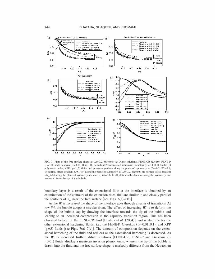
As the Wi is increased the shape of the interface goes through a series of transitions. Atlow Wi, the bubble adopts a circular front. The effect of increasing Wi is to deform theshape of the bubble cap by drawing the interface towards the tip of the bubble andleading to an increased compression in the capillary transition region. This has beenobserved before for the FENE-CR fluid �Bhatara et al. �2004��, and is also true for theother extensional hardening fluids, i.e., the FENE-P, Giesekus �=0.01,0.1�, and XPP�q=5� fluids �see Figs. 7�a�–7�c��. The amount of compression depends on the exten-sional hardening of the fluid and reduces as the extensional hardening is decreased. Asthe Wi is increased further, dilute solutions �FENE-CR, FENE-P and Giesekus �=0.01� fluids� display a meniscus invasion phenomenon, wherein the tip of the bubble is
FIG. 7. Plots of the free surface shape at Ca=0.2, Wi=0.6: �a� Dilute solutions; FENE-CR �L=10�, FENE-P�L=10�, and Giesekus �=0.01� fluids; �b� semidilute/concentrated solutions; Giesekus �=0.1,0.5� fluids; �c�polymeric melts; XPP �q=1,5� fluids; �d� pressure gradient along the plane of symmetry at Ca=0.2, Wi=0.6;�e� normal stress gradient ���xx /�x� along the plane of symmetry at Ca=0.2, Wi=0.6; �f� normal stress gradient���yy /�x� along the plane of symmetry at Ca=0.2, Wi=0.6. In all plots x is the distance along the symmetry linemeasured from the tip of the bubble.
drawn into the fluid and the free surface shape is markedly different from the Newtonian
945FREE SURFACE DISPLACEMENT FLOWS
free surface shape �see Fig. 7�a��. These observations are consistent with experimentalobservations for dilute solutions �Lee et al. �2004��. Furthermore, the meniscus invasionphenomenon is accompanied by a steep local pressure gradient near the tip of the bubblethat is enhanced as Wi is increased �see Fig. 7�d��. This local pressure gradient quicklydissipates as one moves away from the tip of the bubble and is followed by a monotonicdecrease in the pressure �Bhatara et al. �2004��. The semidilute/concentrated solutions�the Giesekus �=0.1,0.5� fluids� and polymeric melts �the XPP �q=1,5� fluids� do notdisplay the phenomenon of meniscus invasion �see Figs. 7�b� and 7�c�� as the normalstresses in the stress boundary layer never get large enough in these fluids due to lack ofsignificant extensional hardening.
It has been shown previously that the presence of elasticity results in three majorcompeting forces at the bubble tip �Bhatara et al. �2004��, a reduction in strain rate due topolymeric restoring forces that result in reduced viscous normal stresses, an increasedpressure drop �see Fig. 7�d��, and accumulation of elastic normal stresses near the centralstagnation line �see Figs. 7�e� and 7�f��. The pressure modification is related to themaximum normal stress in the stress boundary layer in the capillary transition region, andthe steep local pressure gradient is only observed for highly extensional hardening fluids.We expect these forces to play a significant role in the stability characteristics of the flow.Furthermore, the steep local pressure gradient and the accompanying meniscus invasionobserved for the highly extensional hardening fluids is most likely related to the cuspinginstability observed by Lee et al. �2005�.
As stated earlier, we have shown previously, by employing diverging channel walls,that both film thickening and the boundary layer stress formation are largely independentof bulk dynamics �Bhatara et al. �2004��. Furthermore, the film thickness normalized withthe maximum stress in the stress boundary layer in the capillary transition region col-lapses onto a single universal curve �for all diverging channels�, thereby suggesting thatthe film thickening is driven by the maximum stress in the elastic stress boundary layer atthe free surface. We explore this correlation further by plotting the normalized filmthickness for the different extensional hardening fluids, as a function of Wi. Once thestress boundary layer forms �at a Wi of about 0.25�, the normalized film thickness for theFENE-CR �L=10, and L=5� fluid collapse onto a single curve �see Fig. 5�c��. Thenormalized film thickness for the remaining fluids also nearly collapse onto the sameuniversal curve, although a closer examination of the high Wi region shows that there aresome deviations �see Fig. 5�d��. We attribute the deviations in the FENE-P, Giesekus andXPP fluids to the shear thinning viscosity that is absent in the FENE-CR fluid. Thereduction in film thickening because of shear thinning viscosity will be discussed in moredetail in Sec. V.
B. Bypass flow
As in the recirculation flow, the extensional hardening fluids, i.e., the FENE-CR,FENE-P, Giesekus �=0.01,0.1� and XPP �q=5� fluids display a film thickening effectbecause of the presence of elasticity �see Fig. 8�. The flow displays a steady monotonicincrease in film thickness with increasing Wi, with the FENE-CR �L=10� fluid displayingthe highest deviation from the Newtonian film thickness, and the Giesekus �=0.1� fluiddisplaying the least, while both the non-extensional hardening fluids, i.e., the Giesekus�=0.5� and XPP �q=1� fluids display film thinning �see Fig. 8�e��. The increase in filmthickness with the extensional hardening fluids can be attributed to the increase in theextension rate near the bubble tip. The magnitude of the normal stresses near the tip of
the bubble is now larger and can cause a change in the bubble curvature due to the normal
946 BHATARA, SHAQFEH, AND KHOMAMI
stress boundary condition. As shown previously �Bhatara et al. �2004��, the stress profilesobtained for the FENE-CR fluid are qualitatively very different from the stress profiles incase of the recirculation flow. The stresses at the tip of the bubble, i.e., the stagnation
FIG. 8. Contour plots of �xx and �yy and line plots of stress and stress gradients at Ca=1.0 and Wi=0.6: �a�, �b�Giesekus �=0.01�; �c�, �d� XPP �q=5�. s is the distance along the interface measured from the tip of thebubble. �e� Percentage deviation from Newtonian film thickness with Wi at Ca=1.0. �f� Maximum of the traceof the stress tensor ��ii
max� in the stress boundary layer at bubble tip as a function of Wi at Ca=1.0. �g� Filmthickness normalized with �ii
max as a function of Wi at Ca=1.0.
point, are enhanced. Even though an elastic stress boundary layer is observed in the

947FREE SURFACE DISPLACEMENT FLOWS
capillary transition region, the magnitude of normal stresses is much smaller than in therecirculation flow, because the rate of strain is smaller than in the recirculation flow, dueto lack of rapid acceleration of the fluid elements into the thin film region. The formationof stress boundary layers at the stagnation point and in the capillary transition regionoccurs at lower Wi for the bypass flow because of the strong extensional nature of theflow and higher extension rates close to the interface. An additional feature of the stressprofiles is that now both the �xx and �yy components of normal stress are comparable inmagnitude �see Figs. 8�a� and 8�c��. This is because the tangent to the stagnation point, atthe interface, has components of similar magnitude in both the x and y directions, andhence the conformation dyadic has finite and comparable values in both directions. Asexpected, the magnitude of the maximum stress in the stress boundary layer is largest forthe most extensional hardening fluids, i.e., the FENE-CR �L=10� and FENE-P �L=10�fluids and smallest for the least extensional hardening fluid, i.e., the Giesekus �=0.1�fluid. The XPP �q=1� and Giesekus �=0.5� fluids do not display any noticeable normalstresses.
Since the magnitude of normal stresses in the stress boundary layer in the capillarytransition region is small in comparison to that of the recirculation flow, the amount ofcompression of the bubble in the capillary transition region is smaller �see Figs.9�a�–9�c��. However, similar to the recirculation flow, the amount of compression of thebubble in the capillary transition region is largest for the dilute solutions and reduces asthe fluid becomes less extensional hardening. Hence, it is smallest for the concentratedsolution �Giesekus �=0.5�� and the linear polymeric melt �XPP �q=5��. Furthermore,the normal stress balance at the interface now has significant contributions from thenormal stresses at the bubble tip �see Fig. 9�d��. However, unlike the recirculation flow,the normal stresses in the bypass flow for the range of Wi examined never get largeenough for the meniscus invasion phenomenon to occur. This is also corroborated by thefact that elasticity does not significantly alter the local pressure distribution near thebubble tip �see Fig. 9�e��. These observations have been previously reported for theFENE-CR fluid �L=10� �Bhatara et al. �2004�� and are reproduced for the rest of thefluids. As in the recirculation flow, shear thinning or reduction in extensional thickeningresults in reduced stresses in the stress boundary layer, and hence minimizes shapechanges.
Unlike the recirculation flow, the film thickness is now a function of normal stressesformed both in the capillary transition region and at the tip of the bubble. However, sincethe normal stresses at the tip of the bubble are more dominant than the normal stresses inthe capillary transition region �see Figs. 8�b� and 8�d��, the film thickness normalizedwith the maximum of the trace of the stress tensor ��ii
max� at the bubble tip nearly collapsesonto a single curve once boundary layer formation sets in �i.e., for Wi�0.25�. This isillustrated in Fig. 8�g�. As in the recirculation flow, the deviations in this collapse aremore pronounced at higher Wi because of the effect of shear thinning �the normalizedfilm thickness collapses for the FENE-CR �L=10� and FENE-CR �L=5� fluids that havethe same shear viscosity and does not collapse for the remaining fluids that exhibit shearthinning viscosity�. Furthermore, since increasing Ca leads to reduced strain rates andnormal stress, the film thickness in the bypass flow is a stronger function of the shearstress gradients at the wall �see Figs. 8�b� and 8�d�� and hence, more sensitive to theeffects of shear thinning. We account for the reduction in film thickness because of shear
thinning viscosity in Sec. V.
948 BHATARA, SHAQFEH, AND KHOMAMI
V. CORRELATION OF FILM THICKNESS TO THE FLUID RHEOLOGICALPROPERTIES
At this point we have determined that the film thickness is related to two distinctphenomena. First, the extensional hardening of the fluid, as it determines the maximumnormal stress in the stress boundary layers ��xx
max in the recirculation flow, and �iimax in the
bypass flow� and the normal stress gradients ���xx /�x in the recirculation flow, and ��ii /�sin the bypass flow�. Secondly, the amount of shear thinning displayed by the fluid, as itdetermines the viscous drag felt by the fluid elements. In this section, we first show thatwe can predict the maximum normal stress in the stress boundary layer in the capillarytransition region using information from the planar extensional behavior of the fluid and
FIG. 9. Plots of the free surface shape at Ca=1.0, Wi=0.6: �a� Dilute solutions; FENE-CR �L=10�, FENE-P�L=10� and Giesekus �=0.01� fluids; �b� semidilute/concentrated solutions; Giesekus �=0.1,0.5� fluids; �c�polymeric melts; XPP �q=1,5� fluids; �d� normal stress ��xx� along the plane of symmetry at Ca=1.0, Wi=0.6; �e� pressure gradient along the plane of symmetry at Ca=1.0, Wi=0.6. In all plots x is the distance alongthe symmetry line measured from the tip of the bubble.
the flow dynamics. We then develop an accurate correlation between the film thickness

949FREE SURFACE DISPLACEMENT FLOWS
and the maximum normal stress by incorporating the effect of shear thinning �i.e., ac-count for the deviations in the normalized film thickness in Figs. 5�c� and 8�g��.
A. Effect of extensional hardening
For the most extensional hardening fluids �the dilute solutions, FENE-CR �L=10� andFENE-P �L=10��, we start to observe the formation of stress boundary layers and ac-companying film thickening at Wi of about 0.25 at low Ca �Ca�1.0�. We observe a delayin the onset of the boundary layer with respect to Wi, a reduction in the maximum stressin the stress boundary layer and an increase in the thickness of the stress boundary layeras the extensional hardening of the fluid decreases. For fluids that do not display anysignificant extensional hardening we do not observe any noticeable normal stresses. Thisindicates that irrespective of the concentration and/or chain architecture, there exists adirect correlation between the formation of the stress boundary layer and extensionalhardening of the fluid.
Since the flow is inhomogenous and has varying Wi in the flow domain, in order todraw precise correlations, we define an effective Wi, based on the strain rate scaling withfilm thickness, i.e., Wief f =Wi� �b /h�. The local Wi at the interface in the capillary tran-sition region can then be defined as Wiloc=Wief f � �Wint /Wmax�, where Wint is the strain rateat the interface where the boundary layer stresses form, and Wmax is the maximumeffective strain rate. The effective and local Wi are plotted as a function of Wi for eachmodel at a representative value of Ca �Ca=0.2� in Figs. 10�a� and 10�b�, respectively.Approximate scalings for both Wiloc and Wief f can be obtained �i.e., WilocWi0.87 and
0.90
FIG. 10. �a� Plot of the effective Wi as a function of Wi at Ca=0.2. �b� Plot of the local Wi as a function of Wiat Ca=0.2. �c� Plot of the local extensional rate at the interface as a function of Ca. For the viscoelastic fluids,Wi=0.6.
Wief f Wi �. The similar power-law scalings for Wiloc and Wief f indicates that the strain

950 BHATARA, SHAQFEH, AND KHOMAMI
rate at the interface normalized with the maximum strain rate is a weak function of Wi.We calculate the extensional stress based on the local Wi, defined as
�ext = �loc � eloc, �27�
where eloc is the local extensional rate at the interface in the capillary transition region,and �loc is the extensional viscosity obtained from the steady planar extensional rheologydata based on Wiloc. Our simulations indicates that eloc is a strong function of Ca �i.e.,predominantly determined by the flow kinematics� and only weakly dependent on Wi.Consequently, approximate scalings for eloc with Ca can obtained, i.e., in the recirculationflow �Ca�1.0�, at low Ca, elocCa−0.67, and at moderate to high Ca, elocCa−0.41 �seeFig. 10�c��, while in the bypass flow �Ca�1.0�, elocCa−0.36. The scaling at low Careflects the Ca2/3 dependence of the film thickness on Ca �Ro and Homsy �1995��.
The extensional stress calculated using Eq. �27� is plotted in Figs. 11�a� and 11�b� forall fluids, as a function of the actual Wi in the free surface problem, at Ca=0.2. Figure11�a� shows the extensional stresses at a strain rate of 2 �i.e., the strain rate at theinterface in the capillary transition region at Ca=0.05�, while Fig. 11�b� shows the ex-tensional stresses at a strain rate of 0.5 �i.e., the strain rate at the interface in the capillarytransition region at Ca=0.2�. As expected, at both strain rates, the extensional stress is afunction of the choice of the fluid, and is largest for the most extensional hardening fluids�FENE-CR, FENE-P �L=10�� and reduces with decreasing extensional hardening. Thecalculated extensional stress shows the same trend with Wi as the maximum normal stress
FIG. 11. �a� Plot of the calculated extensional stress as a function of Wi at a strain rate of 2. �b� Plot of thecalculated extensional stress as a function of Wi at a strain rate of 0.5. �c� Plot of the ratio of the maximumnormal stress ��xx
max� in the stress boundary layer at Ca=0.2 and the extensional stress calculated at a strain rateof 0.5. �d� Plot of the ratio of the maximum normal stress ��xx
max� in the stress boundary layer at Ca=0.05 and theextensional stress calculated at a strain rate of 2.0. Wi refers to the actual Wi in the free surface problem.
in the stress boundary layer in the capillary transition region.
951FREE SURFACE DISPLACEMENT FLOWS
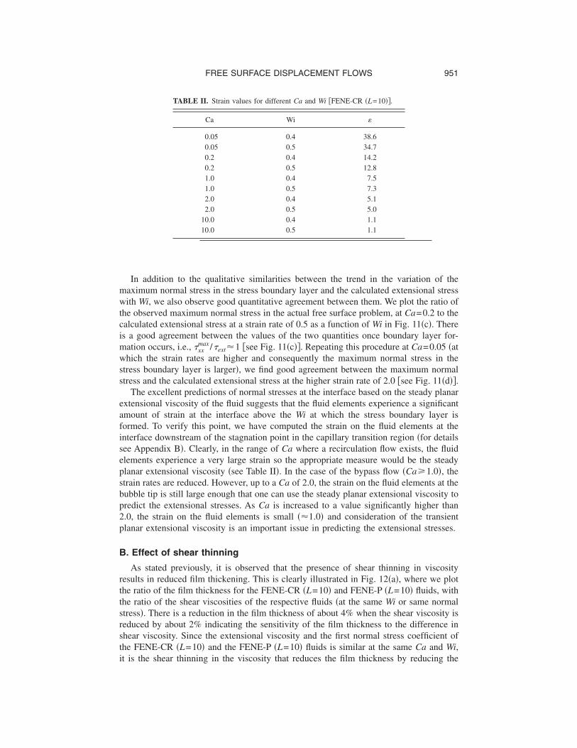
In addition to the qualitative similarities between the trend in the variation of themaximum normal stress in the stress boundary layer and the calculated extensional stresswith Wi, we also observe good quantitative agreement between them. We plot the ratio ofthe observed maximum normal stress in the actual free surface problem, at Ca=0.2 to thecalculated extensional stress at a strain rate of 0.5 as a function of Wi in Fig. 11�c�. Thereis a good agreement between the values of the two quantities once boundary layer for-mation occurs, i.e., �xx
max /�ext1 �see Fig. 11�c��. Repeating this procedure at Ca=0.05 �atwhich the strain rates are higher and consequently the maximum normal stress in thestress boundary layer is larger�, we find good agreement between the maximum normalstress and the calculated extensional stress at the higher strain rate of 2.0 �see Fig. 11�d��.
The excellent predictions of normal stresses at the interface based on the steady planarextensional viscosity of the fluid suggests that the fluid elements experience a significantamount of strain at the interface above the Wi at which the stress boundary layer isformed. To verify this point, we have computed the strain on the fluid elements at theinterface downstream of the stagnation point in the capillary transition region �for detailssee Appendix B�. Clearly, in the range of Ca where a recirculation flow exists, the fluidelements experience a very large strain so the appropriate measure would be the steadyplanar extensional viscosity �see Table II�. In the case of the bypass flow �Ca�1.0�, thestrain rates are reduced. However, up to a Ca of 2.0, the strain on the fluid elements at thebubble tip is still large enough that one can use the steady planar extensional viscosity topredict the extensional stresses. As Ca is increased to a value significantly higher than2.0, the strain on the fluid elements is small �1.0� and consideration of the transientplanar extensional viscosity is an important issue in predicting the extensional stresses.
B. Effect of shear thinning
As stated previously, it is observed that the presence of shear thinning in viscosityresults in reduced film thickening. This is clearly illustrated in Fig. 12�a�, where we plotthe ratio of the film thickness for the FENE-CR �L=10� and FENE-P �L=10� fluids, withthe ratio of the shear viscosities of the respective fluids �at the same Wi or same normalstress�. There is a reduction in the film thickness of about 4% when the shear viscosity isreduced by about 2% indicating the sensitivity of the film thickness to the difference inshear viscosity. Since the extensional viscosity and the first normal stress coefficient ofthe FENE-CR �L=10� and the FENE-P �L=10� fluids is similar at the same Ca and Wi,
TABLE II. Strain values for different Ca and Wi �FENE-CR �L=10��.
Ca Wi �
0.05 0.4 38.60.05 0.5 34.70.2 0.4 14.20.2 0.5 12.81.0 0.4 7.51.0 0.5 7.32.0 0.4 5.12.0 0.5 5.0
10.0 0.4 1.110.0 0.5 1.1
it is the shear thinning in the viscosity that reduces the film thickness by reducing the

952 BHATARA, SHAQFEH, AND KHOMAMI
shear stress gradients at the wall or the viscous drag felt by the fluid elements �Ro andHomsy �1995��.
In order to account for shear thinning in the extensional hardening, shear thinningfluids, namely, the FENE-P, Giesekus �=0.01,0.1� and XPP �q=5� fluids, we define aneffective Ca based on a normalization of the viscosity with the shear viscosity at the wallshear rate �also the maximum shear rate�, since the shear rate at the wall predominantlydetermines the amount of fluid dragged into the thin film region. The effective Ca, hence,
FIG. 12. �a� Plot of the ratio of film thickness for FENE-P �L=10� and FENE-CR �L=10� with the ratio ofrespective shear viscosities at Ca=0.2. �b�, �c� Plot of the ratio of the maximum normal stress ��xx
max� in the stressboundary layer at the effective Ca and the extensional stress calculated for a strain rate of 0.5, �d� Plot of filmthickness normalized with �xx
max at the effective Ca. �e�, �f� Plot of the ratio of the maximum normal stress ��xx�in the stress boundary layer at the effective Ca and the extensional stress calculated for a strain rate of 2.0. Wirefers to the actual Wi in the free surface problem.
is defined as
953FREE SURFACE DISPLACEMENT FLOWS
Caef f = Ca � ��wall, �28�
where ��wallis the dimensionless shear viscosity at the wall shear rate, and is obtained
from the steady shear rheological predictions of that particular fluid. For a particular Wi,we suggest that the normal stress corresponding to Caef f can be correlated to the exten-sional stress calculated above. Figures 12�b� and 12�c� show the ratio of the maximumnormal stress corresponding to Caef f to the calculated extensional stress �at a strain rate of0.5� as a function of Wi. We notice a marked improvement in the agreement between �xx
max
and the calculated extensional stress. Furthermore, the film thickness normalized with�xx
max corresponding to Caef f now collapses onto a single curve for all fluids �see Fig.12�d��, thereby establishing that for Wi greater than the critical Wi for boundary layerformation, the film thickness scales with the maximum normal stress provided shearthinning is accounted for. This procedure is repeated at Ca=0.05 and again there is amarked improvement in the agreement between �xx
max and the calculated extensional stressat a strain rate of 2.0 �see Figs. 12�e� and 12�f��.
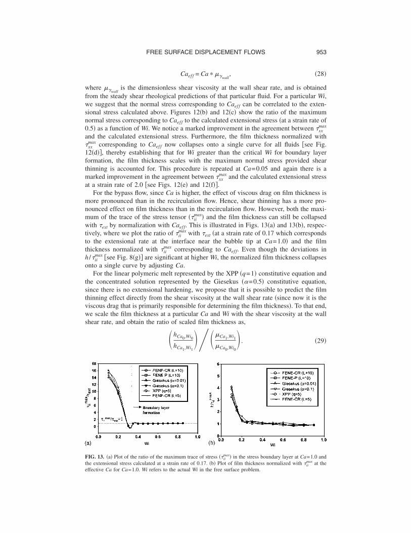
For the bypass flow, since Ca is higher, the effect of viscous drag on film thickness ismore pronounced than in the recirculation flow. Hence, shear thinning has a more pro-nounced effect on film thickness than in the recirculation flow. However, both the maxi-mum of the trace of the stress tensor ��ii
max� and the film thickness can still be collapsedwith �ext by normalization with Caef f. This is illustrated in Figs. 13�a� and 13�b�, respec-tively, where we plot the ratio of �ii
max with �ext �at a strain rate of 0.17 which correspondsto the extensional rate at the interface near the bubble tip at Ca=1.0� and the filmthickness normalized with �ii
max corresponding to Caef f. Even though the deviations inh /�ii
max �see Fig. 8�g�� are significant at higher Wi, the normalized film thickness collapsesonto a single curve by adjusting Ca.
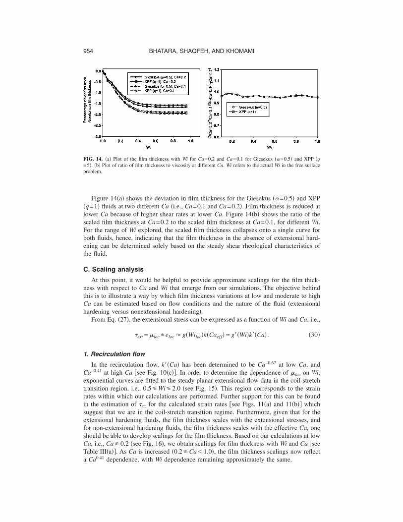
For the linear polymeric melt represented by the XPP �q=1� constitutive equation andthe concentrated solution represented by the Giesekus �=0.5� constitutive equation,since there is no extensional hardening, we propose that it is possible to predict the filmthinning effect directly from the shear viscosity at the wall shear rate �since now it is theviscous drag that is primarily responsible for determining the film thickness�. To that end,we scale the film thickness at a particular Ca and Wi with the shear viscosity at the wallshear rate, and obtain the ratio of scaled film thickness as,
�hCa0,Wi0
hCa1,Wi1
���Ca1,Wi1
�Ca0,Wi0
� . �29�
FIG. 13. �a� Plot of the ratio of the maximum trace of stress ��iimax� in the stress boundary layer at Ca=1.0 and
the extensional stress calculated at a strain rate of 0.17. �b� Plot of film thickness normalized with �iimax at the
effective Ca for Ca=1.0. Wi refers to the actual Wi in the free surface problem.
954 BHATARA, SHAQFEH, AND KHOMAMI
Figure 14�a� shows the deviation in film thickness for the Giesekus �=0.5� and XPP�q=1� fluids at two different Ca �i.e., Ca=0.1 and Ca=0.2�. Film thickness is reduced atlower Ca because of higher shear rates at lower Ca. Figure 14�b� shows the ratio of thescaled film thickness at Ca=0.2 to the scaled film thickness at Ca=0.1, for different Wi.For the range of Wi explored, the scaled film thickness collapses onto a single curve forboth fluids, hence, indicating that the film thickness in the absence of extensional hard-ening can be determined solely based on the steady shear rheological characteristics ofthe fluid.
C. Scaling analysis
At this point, it would be helpful to provide approximate scalings for the film thick-ness with respect to Ca and Wi that emerge from our simulations. The objective behindthis is to illustrate a way by which film thickness variations at low and moderate to highCa can be estimated based on flow conditions and the nature of the fluid �extensionalhardening versus nonextensional hardening�.
From Eq. �27�, the extensional stress can be expressed as a function of Wi and Ca, i.e.,
�ext = �loc � eloc g�Wiloc�k�Caef f� = g��Wi�k��Ca� . �30�
1. Recirculation flow
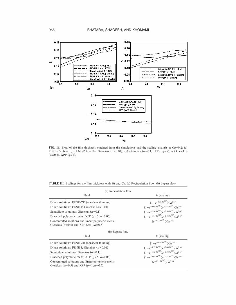
In the recirculation flow, k��Ca� has been determined to be Ca−0.67 at low Ca, andCa−0.41 at high Ca �see Fig. 10�c��. In order to determine the dependence of �loc on Wi,exponential curves are fitted to the steady planar extensional flow data in the coil-stretchtransition region, i.e., 0.5�Wi�2.0 �see Fig. 15�. This region corresponds to the strainrates within which our calculations are performed. Further support for this can be foundin the estimation of �xx for the calculated strain rates �see Figs. 11�a� and 11�b�� whichsuggest that we are in the coil-stretch transition regime. Furthermore, given that for theextensional hardening fluids, the film thickness scales with the extensional stresses, andfor non-extensional hardening fluids, the film thickness scales with the effective Ca, oneshould be able to develop scalings for the film thickness. Based on our calculations at lowCa, i.e., Ca�0.2 �see Fig. 16�, we obtain scalings for film thickness with Wi and Ca �seeTable III�a��. As Ca is increased �0.2�Ca�1.0�, the film thickness scalings now reflect
0.41
FIG. 14. �a� Plot of the film thickness with Wi for Ca=0.2 and Ca=0.1 for Giesekus �=0.5� and XPP �q=5�. �b� Plot of ratio of film thickness to viscosity at different Ca. Wi refers to the actual Wi in the free surfaceproblem.
a Ca dependence, with Wi dependence remaining approximately the same.

955FREE SURFACE DISPLACEMENT FLOWS
2. Bypass flow
In the bypass flow �Ca�1.0� we again obtain scalings for film thickness with Wi andCa �see Fig. 17 and Table III�b��. We observe these scalings to hold true for values of Cathat are not significantly greater than 1.0. As the value of Ca is increased, the strain at thetip of the bubble decreases �see Table II�. For Ca=10.0, the strain is low enough ��1.0� for the transient characteristics to be important. Hence, we expect the scalinganalysis based on steady data to be insufficient in predicting film thickness at such highvalues of Ca.
VI. CONCLUSION
We have inspected the effect of viscoelasticity on the interfacial dynamics of a Hele-Shaw cell free surface displacement flow. The FENE-CR �extensional hardening, con-stant shear viscosity, shear thinning first normal stress coefficient� and the FENE-P �ex-tensional hardening, shear thinning viscosity and shear thinning first normal stresscoefficient� constitutive equations are used to model dilute polymeric solutions. TheGiesekus constitutive equation �=0.01,0.1,0.5� is used to model dilute, semidilute andconcentrated solutions. For all values of , the model shows shear thinning viscosity andshear thinning first and second normal stress coefficients and for two of the values�0.01, 0.1�, the model displays significant extensional hardening. The XPP constitutiveequation is used to model polymeric melts. Linear polymeric melts are represented bysetting q=1, while branched polymeric melts are represented by setting q=5. For bothq=1 and q=5, the model shows shear thinning viscosity and shear thinning first and
FIG. 15. Exponential fits to the steady planar rheological data. Extensional viscosity in steady planar exten-sional flow: �a� FENE-CR �L=5,10�, FENE-P �L=10�; �b� Giesekus �=0.01,0.1�; �c� XPP �q=5,=0.06�.Shear viscosity in steady shear flow: �d� Giesekus �=0.5�; XPP �q=1,=0.5�.
second normal stress coefficients. In steady planar extensional flow the XPP �q=5� model
956 BHATARA, SHAQFEH, AND KHOMAMI
TABLE III. Scalings for the film thickness with Wi and Ca. �a� Recirculation flow; �b� bypass flow.
�a� Reciculation flowFluid h �scaling�
Dilute solutions: FENE-CR �nonshear thinning� �1−e−0.68Wi0.87�Ca0.67
Dilute solutions: FENE-P, Giesekus �=0.01� �1−e−0.68Wi0.87�e−0.42Wi0.87
Ca0.67
Semidilute solutions: Giesekus �=0.1� �1−e−1.16Wi0.87�e−0.38Wi0.87
Ca0.67
Branched polymeric melts: XPP �q=5, =0.06� �1−e−1.14Wi0.87�e−0.38Wi0.87
Ca0.67
Concentrated solutions and linear polymeric melts:Giesekus �=0.5� and XPP �q=1,=0.5�
�e−0.31Wi0.87�Ca0.67
�b� Bypass flowFluid h �scaling�
Dilute solutions: FENE-CR �nonshear thinning� �1−e−0.59Wi0.87�Ca0.67
Dilute solutions: FENE-P, Giesekus �=0.01� �1−e−0.59Wi0.87�e−0.40Wi0.87
Ca0.36
Semidilute solutions: Giesekus �=0.1� �1−e−1.12Wi0.87�e−0.38Wi0.87
Ca0.67
Branched polymeric melts: XPP �q=5, =0.06� �1−e−0.98Wi0.87�e−0.38Wi0.87
Ca0.67
Concentrated solutions and linear polymeric melts:Giesekus �=0.5� and XPP �q=1,=0.5�
�e−0.31Wi0.87�Ca0.36
FIG. 16. Plots of the film thickness obtained from the simulations and the scaling analysis at Ca=0.2: �a�FENE-CR �L=10�, FENE-P �L=10�, Giesekus �=0.01�; �b� Giesekus �=0.1�, XPP �q=5�; �c� Giesekus�=0.5�, XPP �q=1�.
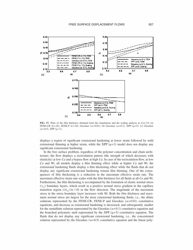
957FREE SURFACE DISPLACEMENT FLOWS
displays a region of significant extensional hardening at lower strain followed by mildextensional thinning at higher strain, while the XPP �q=1� model does not display anysignificant extensional hardening.
In the free surface problem, regardless of the polymer concentration and chain archi-tecture, the flow displays a recirculation pattern �the strength of which decreases withelasticity� at low Ca and a bypass flow at high Ca. In case of the recirculation flow, at lowCa and Wi, all models display a film thinning effect while at higher Ca and Wi, theextensional hardening fluids display a film thickening effect while the fluids that do notdisplay any significant extensional hardening remain film thinning. One of the conse-quences of film thickening is a reduction in the maximum effective strain rate. Themaximum effective strain rate scales with the film thickness for all fluids at all Ca and Wi.Furthermore, the film thickening is accompanied by the formation of elastic normal stress��xx� boundary layers, which result in a positive normal stress gradient in the capillarytransition region ���xx /�x�0� in the flow direction. The magnitude of the maximumstress in the stress boundary layer increases with Wi. Both the film thickness and maxi-mum normal stress are largest for the most extensional hardening fluids, i.e., the dilutesolutions represented by the FENE-CR, FENE-P and Giesekus �=0.01� constitutiveequations, and decrease as extensional hardening is decreased, and subsequently smallerfor the semidilute solution represented by the Giesekus �=0.1� constitutive equation andthe branched polymeric melt represented by the XPP �q=5� constitutive equation. Thefluids that do not display any significant extensional hardening, i.e., the concentrated
FIG. 17. Plots of the film thickness obtained from the simulations and the scaling analysis at Ca=1.0: �a�FENE-CR �L=10�, FENE-P �L=10�, Giesekus �=0.01�; �b� Giesekus �=0.1�, XPP �q=5�; �c� Giesekus�=0.5�, XPP �q=1�.
solution represented by the Giesekus �=0.5� constitutive equation and the linear poly-
958 BHATARA, SHAQFEH, AND KHOMAMI
meric melt represented by the XPP �q=1� constitutive equation, display film thinning andno noticeable normal stresses.
In the recirculation flow, we observe that the film thickness scales with the maximumnormal stress in the stress boundary layer in the capillary transition region near the freesurface. Specifically, for the extensional hardening, nonshear thinning fluids, i.e., theFENE-CR �L=5� and �L=10� fluids, the film thickness normalized with the maximumnormal stress in the stress boundary layer, collapses onto a single curve. For the exten-sional hardening, shear thinning fluids, i.e., the FENE-P �L=10�, Giesekus �=0.01,0.1�, and XPP �q=5� fluids, there are some slight deviations from this collapse.This is because film thickening is reduced by shear thinning which lowers the viscousforces that drag fluid into the thin film region. We show that shear thinning can beaccounted for by defining an effective Ca by normalizing the viscosity with the shearviscosity at the wall shear rate. For a given Wi, the film thickness normalized with themaximum normal stress at the effective Ca now collapses onto a single curve for theaforementioned fluids. For the fluids that are shear thinning but not extensional harden-ing, it is observed that the film thickness scaled with the shear viscosity at the wall shearrate collapses onto a single curve, indicating that the film thickness solely depends on theviscous drag felt by the fluid elements.
For the recirculation flow, we correlate the measured film thickness and normalstresses to the rheological behavior of the fluids. Since the flow is planar extensional atthe interface in the capillary transition region where the stress boundary layer forms, it ispossible to calculate the maximum normal stress in the stress boundary layer using theextensional viscosity and extensional rate at the interface. Calculation of extensionalstress based on the planar extensional rheology shows good agreement with the maxi-mum normal stress in the stress boundary layer, indicating that given the planar exten-sional rheological behavior of a fluid, one can estimate the stresses that would result inthe free surface displacement problem. In order to perform an accurate calculation, de-tailed knowledge of the flow kinematics at the interface and the wall is required. How-ever, one can obtain good approximations for film thickness using the correlations ob-tained from our simulations.
For the bypass flow, the film thickness nearly scales with the maximum of the trace ofthe stress tensor at the tip of the bubble. The effect of shear thinning viscosity on thescaling is more pronounced because of reduced strain rates and normal stresses at thehigher Ca at which the bypass flow occurs. However, as in the recirculation flow, thedeviations in the collapse because of shear thinning can be accounted for by normalizingthe shear viscosity with the viscosity at the wall shear rate. Furthermore, for Ca close to1.0, the stress at the tip of the bubble can be estimated from the steady planar extensionalrheology, and approximate correlations for film thickness can be determined. However, asthe value of Ca becomes significantly greater than 1.0 �Ca10.0�, we expect the tran-sient characteristics to be important and need to be taken into account in determining thefilm thickness.
This work provides a comprehensive study of the effect of concentration and chainarchitecture of polymeric fluids on observed film thickness and normal stresses in asteady free surface displacement flow, and provides a basis for further work on under-standing the effects of viscoelasticity on the interfacial dynamics of free surface displace-ment flows.
ACKNOWLEDGMENTS
E.S.G.S. and B.K. would like to thank NSF for supporting this work through Grants
0090428 and 0089502, respectively.
959FREE SURFACE DISPLACEMENT FLOWS
APPENDIX A: INLET CONDITIONS FOR DIFFERENT MODELS
FENE-P, Giesekus: The inlet conditions for the FENE-P and Giesekus model are morecomplicated due to the coupling of the out of plane components of the configurationaltensor with the in-plane deformation.
For the sake of simplicity, the following abbreviations are used:
Cxx − Cyy = n1, �A1�
Czz − Cyy = n2, �A2�
Cxy = n3, �A3�
Czz = 1, �A4�
where
n1 =2n2�1 − n2�
�1 − n2�, �A5�
n3 =�1 − n2�2
1 + �1 − 2�n2Wi, �A6�
n2 =1 − n4
1 + �− 2�n4, �A7�
n4 =� 1
8�1 − �Wi2��1 + 16�1 − �Wi2 − 1� . �A8�
Equation �A13� is introduced into Eq. �A12� for calculating n2, and using Eqs. �A10�and �A11�, n1 and n3 are obtained. By setting =0, the inlet conditions for FENE-P areobtained.
XPP: For the XPP model it is not possible to write an analytically tractable form for�0. However, it is possible to write analytical expressions for =0. Furthermore, sincein simple steady shear flow, the rheological behavior of the XPP model is insensitive to, we can use the inlet conditions corresponding to =0 for nonzero :
�xx = 3GWi� 1
�1 − WiSxy�2��2Wi��b�2 + � 1
Wi�
2Wi2��b�2 + 3� , �A9�
�yy = �zz = 3GWi� 1
�1 − WiSxy�2�� 1
2Wi2��b�2 + 3� , �A10�
�xy = 3GWi� 1
�1 − WiSxy�2�� 1
2Wi2 +�b � , �A11�
3
960 BHATARA, SHAQFEH, AND KHOMAMI
Sxy =Wi
2Wi2 +�b
3
. �A12�
APPENDIX B: STRAIN CALCULATIONS
In order to calculate the effective strain felt by a fluid element at the free surface in thecapillary transition region where the stress boundary layer has formed, the strain rate isintegrated with respect to time along the path on the free surface. Hence the effectivestrain can be calculated as
� = 0
�
�̇�t�dt . �B1�
In the case of the recirculation flow, at t=0 the fluid element is at the stagnation point atthe interface, and at t=� the fluid element is located at the end of the capillary transitionregion. For the bypass flow, at t=0 the fluid element is present at the tip of the bubble,and at t=� the fluid element is located at the beginning of the capillary transition region.
Using this method of calculation, for Ca�1.0 and for all values of Wi�Wicrit, whereWicrit is the critical Wi for onset of boundary layer formation, we determine the fluidelements to have experienced effective strains which are large enough for the steadyanalysis to be applicable �see Table II�.
References
Arora, K., V. Ganesan, R. Sureshkumar, and B. Khomami, “Linear dynamics of unidirectional shear flow of
linear and branched polymeric melts: Eigenspectrum and stability analysis,” J. Non-Newtonian Fluid Mech.
121, 101–115 �2004�.Bhatara, G., E. S. G. Shaqfeh, and B. Khomami, “Influence of viscoelasticity on the interfacial dynamics of air
displacing fluid flows—A computational study,” J. Non-Newtonian Fluid Mech. 122, 313–332 �2004�.Bird, R. B., R. C. Armstrong, and O. Hassager, Dynamics of Polymeric Liquids �Wiley, New York, 1987�.Bird, R. B., P. J. Dotson, and N. L. Johnson, “Polymer solution rheology based on a finitely extensible
bead-spring chain model,” J. Non-Newtonian Fluid Mech. 7, 213–235 �1980�.Bonn, D., H. Kellay, M. Braunlich, M. Ben Amar, and J. Meunier, “Viscous fingering in complex fluids,”
Physica A 220, 60–73 �1995�.Bretherton, F. P., “The motion of long bubbles in tubes,” J. Fluid Mech. 10, 166–188 �1961�.Brooks, A. N., and T. J. R. Hughes, “Streamline upwind-Petrov Galerkin formulations for convection domi-
nated flows with particular emphasis on the incompressible Navier-Stokes equations,” Comput. Methods
Appl. Mech. Eng. 32, 199–259 �1982�.Burghardt, W. R., J. M. Li, B. Khomami, and B. Yang, “Uniaxial extensional characterization of a shear
thinning fluid using axisymmetric flow birefringence,” J. Rheol. 43, 147–165 �1999�.Cairncross, R. A., P. R. Schunk, T. A. Baer, R. R. Rao, and P. A. Sackinger, “A finite element method for free
surface flows of incompressible fluids in three dimensions. Part I. Boundary fitted mesh motion,” Int. J.
Numer. Methods Fluids 33, 375 �2000�.Chilcott, M. D., and J. M. Rallison, “Creeping flow of dilute polymer solutions past cylinders and spheres,” J.
Non-Newtonian Fluid Mech. 29, 381–432 �1988�.Cox, B. G., “On driving a viscous fluid out of a tube,” J. Fluid Mech. 14, 81–96 �1962�.Coyle, D. J., C. W. Macosko, and L. E. Scriven, “Reverse roll coating of non-Newtonian liquids,” J. Rheol. 34,
615–636 �1990�.

961FREE SURFACE DISPLACEMENT FLOWS
deGennes, P. G., “Reptation of a polymer chain in the presence of fixed obstacles,” J. Chem. Phys. 55, 572–579
�1971�.Doi, M., and S. F. Edwards, The Theory of Polymer Dynamics �Oxford, New York, 1986�.Giavedoni, M. D., and F. A. Saita, “The axisymmetric and plane cases of a gas phase steadily displacing a
Newtonian liquid—A simultaneous solution of the governing equations,” Phys. Fluids 8, 2420–2432
�1997�.Giesekus, H., “A simple constitutive equation for polymer fluids based on the concept of deformation-
dependent tensorial mobility,” J. Non-Newtonian Fluid Mech. 11, 69–109 �1982�.Grillet, A. M., A. G. Lee, and E. S. G. Shaqfeh, “Observation of ribbing instabilities in elastic fluid flows with
gravity stabilization,” J. Fluid Mech. 399, 49–83 �1999�.Guenette, R., and M. Fortin, “A new mixed finite element method for computing viscoelastic flows,” J. Non-
Newtonian Fluid Mech. 60, 27–52 �1995�.Huzyak, P. C., and K. W. Koelling, “The penetration of a long bubble through a viscoelastic fluid in a tube,” J.
Non-Newtonian Fluid Mech. 71, 73–88 �1997�.Larson, R. G., “Instabilities in viscoelastic flows,” Rheol. Acta 31, 213–234 �1992�.Lee, A. G., E. S. G. Shaqfeh, and B. Khomami, “A study of viscoelastic free surface flows by the finite element
method: Hele-Shaw and slot coating flows,” J. Non-Newtonian Fluid Mech. 108, 327–362 �2002�.Lee, A. G., E. S. G. Shaqfeh, and B. Khomami, “Viscoelastic Effects on Interfacial Dynamics in Air-Fluid
Displacement under Gravity Stabilization,” J. Fluid Mech. 531, 59–83 �2005�.Lidner, A., D. Bonn, E. Corvera Poire’, M. B. Amar, and J. Meunier, “Viscous fingering in non-Newtonian
fluids,” J. Fluid Mech. 469, 237–256 �2002�.Milner, S. T., and T. C. B. Mcleish, “Reptation and contour length fluctuations in melts of linear polymers,”
Phys. Rev. Lett. 81, 725–728 �1998�.Noda, I., Y. Yamada, and M. Nagasawa, “The rate of shear dependence of the intrinsic viscosity of monodis-
perse polymer,” J. Phys. Chem. 72, 2890–2898 �1968�.Oene, H. V., and L. H. Cragg, “Shear dependence of reduced viscosity-concentration slope constant,” J. Polym.
Sci. 57, 209–227 �1962�.Park, C. W., and G. M. Homsy, “Two-phase displacement in Hele Shaw cells: theory,” J. Fluid Mech. 139,
291–308 �1984�.Pasquali, M., and L. E. Scriven, “Free surface flows of polymer solutions with models based on the conforma-
tion tensor,” J. Non-Newtonian Fluid Mech. 108, 363–409 �2002�.Pearson, J. R. A., “The instability of uniform viscous flow under rollers and spreaders,” J. Fluid Mech. 7,
481–495 �1960�.Pitts, E., and J. Greiller, “The flow of thin films between rollers,” J. Fluid Mech. 11, 33–50 �1961�.Poslinski, A. J., P. R. Oehler, and V. K. Stokes, “Isothermal gas-assisted displacement of viscoplastic liquids in
tubes,” Polym. Eng. Sci. 35, 877–892 �1995�.Rabaud, M., S. Michalland, and Y. Couder, “Dynamical regimes of directional viscous fingering: Spatiotempo-
ral chaos and wave propogation,” Phys. Rev. Lett. 64, 184–187 �1990�.Reinelt, D. A., and P. G. Saffman, “The penetration of a finger into a viscous fluid into a channel and tube,”
SIAM �Soc. Ind. Appl. Math.� J. Sci. Stat. Comput. 6, 542–561 �1985�.Ro, J. S., and G. M. Homsy, “Viscoelastic free surface flows: thin film hydrodynamics of Hele-Shaw and dip
coating flows,” J. Non-Newtonian Fluid Mech. 57, 203–225 �1995�.Ruschak, K. J., “Coating flows,” J. Fluid Mech. 17, 65–89 �1985�.Sackinger, P. A., P. R. Schunk, and R. R. Rao, “A Newton-Rhapson pseudo-solid domain mapping technique for
free and moving boundary problems: a finite element implementation,” J. Comput. Phys. 125, 83–103
�1996�.Shaqfeh, E. S. G., “Purely elastic instabilities in viscoelastic flows,” Annu. Rev. Fluid Mech. 28, 129–185
�1995�.Sullivan, T. M., and S. Middleman, “Roll coating in the presence of a fixed constraining boundary,” Chem. Eng.
Commun. 3, 469–482 �1979�.Sureshkumar, R., A. Beris, and R. Handler, “Direct numerical simulation of the turbulent channel flow of a
polymer solution,” Phys. Fluids 9, 433–468 �1997�.

962 BHATARA, SHAQFEH, AND KHOMAMI
Szady, M. J., T. R. Salamon, A. W. Liu, D. E. Bornside, R. C. Armstrong, and R. A. Brown, “A new mixed
finite element method for viscoelastic flows generated by differential constitutive equations,” J. Non-
Newtonian Fluid Mech. 59, 215–243 �1995�.Talwar, K. K., and B. Khomami, “Application of higher order finite element methods to viscoelastic flow in
porous media,” J. Rheol. 36, 1377–1416 �1992�.Taylor, G. I., “Deposition of a viscous fluid on the walls of a tube,” J. Fluid Mech. 10, 161–165 �1961�.Verbeeten, W. M. H., G. W. M. Peters, and F. P. T. Baaijens, “Differential constitutive equations for polymer
melts: The extended Pom-Pom model,” J. Rheol. 45, 823–843 �2001�.Verbeeten, W. M. H., G. W. M. Peters, and F. P. T. Baaijens, “Viscoelastic analysis of complex polymer melts
flows using the extended Pom-Pom model,” J. Non-Newtonian Fluid Mech. 108, 301–326 �2002�.Yurun, F., and M. J. Crochet, “Higher order finite element method for steady viscoelastic flows,” J. Non-
Newtonian Fluid Mech. 57, 283–311 �1995�.