The Interpretation Of Physically Based Climate Models ... · PDF fileThe Interpretation Of Physically Based Climate Models: Statistics .vs. Physics .vs. Philosophy D A Stainforth1,2

The Interpretation Of Physically Based Climate Models: Statistics .vs. Physics .vs. Philosophy

D A Stainforth1,2

INTEGRATE Meeting Lund University

14th November 2016

1Grantham Research Institute and Centre for the Analysis of Timeseries, London School of Economics, 2Dept. of Physics, Warwick University,

Acknowledgements: L A Smith, M R Allen and a cast of thousands

Papers discussed

Layout

• An introduction to global climate models (GCMs). • Perturbed physics ensembles and climateprediction.net • Key elements of the climate prediction challenge. • Challenges in the design and interpretation of multi-model

ensembles (MMEs) and perturbed physics ensembles (PPEs)

19 levels in

atmosphere

20 levels

in ocean

2.5

lat 3.75 long

1.25

1.25

-5km

Complex Climate Models [Global Circulation Models]

Complex Climate Models / Global Circulation Models (GCMs)

DDtρ ρ= − ∇•u

1p

DT Dpc QDt Dtρ

= +

p RTρ=

22D pDt

ηρ ρ

−∇= − − − ∇

uΩ u g u x

Figure source: Emily Black / NERC

Momentum equation

Conservation of mass

Conservation of energy

Ideal gas equation (Eqn of state)

GCMs: Parameterizations

• Clouds • Precipitation • Radiation • Gravity waves • Convection • Land surface • (Carbon cycle) • (Sea ice) • ((Ice sheets))

• Missing: ocean/atmospheric chemistry , ecosystems, stratosphere …

Models Included in the Fifth Coupled Model Intercomparison Project (CMIP5) and used in the IPCC Fifth Assessment report:

Even amongst the most up-to-date models there are a wide variety of different resolutions and different levels of complexity in parameterization schemes.

How Many GCMs are there?

Source: IPCC WG1 AR5 Chapter 9, Table 9.1 For detailed model specifications look at Table 9.A.1

MSc Climate Change: Science, Economics and Policy

Model Simulations from the IPCC Fifth Assessment Report (AR5)

Source: WG1 SPM IPCC 2013

All temperatures are shown relative to the 1986-2005 average Add about 0.6 to get the value relative to pre-industrial

8

Presentation of Global Mean Temperature Change


9

Source: WG1 Ch 12 IPCC 2013

Source: WG1 Ch 9 IPCC 2013

Surface Temperature


10

Precipitation


11

Regional / Local Predictions An Area of Significant Effort

The North American Regional Climate Change Assessment Program (NARCCAP) aims to “investigate uncertainties in regional scale projections of future climate and generate climate change scenarios for use in impacts research.” http://www.narccap.ucar.edu/about/index.html

2080s: 90% probability level: very unlikely to be greater than

2080s : 67% probability level: unlikely to be greater than

Change in Wettest Day in Summer Medium (A1B) scenario

UKCP09: NARCCAP:

“The UK Climate Projections (UKCP09) provide climate information designed to help those needing to plan how they will adapt to a changing climate. The data is focussed on the UK,” “UKCP09 provides future climate projections for land and marine regions.” “They assign probabilities to different future climate outcomes. “ http://ukclimateprojections.defra.gov.uk

ENV.2011.1.1.6-1 “The proposed research activities should […] quantify the impacts of climate change in selected areas of Europe […] arising from a global averaged surface temperature change of 2°C from preindustrial level.” ftp://ftp.cordis.europa.eu/pub/fp7/docs/wp/cooperation/environment/f-wp-201101_en.pdf

€7M European Call:

Tebaldi et al.., JoC, 2005

Stott et al.., GRL, 2006

UK Climate Projections 2009 (2018)

UK Climate Projections 2009: Change in Wettest Day in Summer in A1B scenario

2080s: 90% probability level: very unlikely to be greater than

2080s : 67% probability level: unlikely to be greater than

“The UK Climate Projections (UKCP09) provide climate information designed to help those needing to plan how they will adapt to a changing climate. The data is focussed on the UK,” “UKCP09 provides future climate projections for land and marine regions.” “They assign probabilities to different future climate outcomes. “ http://ukclimateprojections.defra.gov.uk

Critical Assessments:

Frigg, R., L.A. Smith, D. A. Stainforth, The Myopia of Imperfect Climate Models: The Case of UKCP09, Philosophy of Science, 2013.

Frigg, R., L.A. Smith, D. A. Stainforth, “An assessment of the foundational assumptions in high-resolution climate projections: the case of UKCP09”, Synthese, 2015.

Model Differences: Individual Model

Results: Temperature

[CMIP3]

Source: IPCC AR4 WG1 Supplementary Information

Model differences: Individual Model Errors

in Annual Mean Temperature

[CMIP3]

Source: IPCC AR4 WG1 Supplementary Information S8.1b

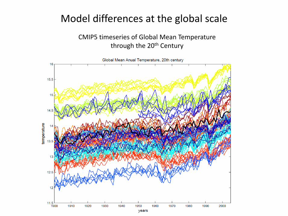
Model differences at the global scale CMIP5 timeseries of Global Mean Temperature

through the 20th Century

Climateprediction.net History

• Climateprediction.net is a project which engages the public to use spare capacity on their PCs to do climate simulations.

• Conceived in 1998 by Myles Allen • Development began in earnest in 2000 when I joined Myles to

do model and software development and experimental design.

• Launched in 2003 • First results published in 2005. • Includes a wide variety of experiments.

I’m presenting results from the first experiment which has by far the largest exploration of model uncertainty of any climateprediction.net or other climate model experiment.

Climateprediction.net: The first (slab) Experiment

Unified Model with thermodynamic ocean. (HadSM3)

15 yr spin-up 15 yr, base case CO2

15 yr, 2 x CO2

Derived fluxes

Diagnostics from final 8 yrs.

Calibration

Control

Double CO2

Stan

dard

mod

el

set-u

p

Perturbed Physics

Ensemble

Initial Condition Ensemble

Grand Ensem

ble

10000s 10s P1 Low High Stnd

Stnd

Low

High P2

Parameter Space, Sampling Strategy and the need for large ensembles

P1 Low High Stnd

Stnd

Low

High P2 • There are hundreds of uncertain parameters in

a GCM. • To study them one at a time is easy. • But they interact non-linearly so we need to

explore multiple perturbations simultaneously.

No. of parameters

One at a time

All combinations

1 3 3 2 5 9 3 7 27 6 13 729 21 42 1010

Required number of simulations:

Public Resource Distributed Computing Projects (PRDC – aka Volunteer Computing)

Climateprediction.net

GIMPS SETI@home Folding@home

LHC@home Einstein@home Lifemapper

Find-a-drug FightAIDS@home Evolution@home

Eon Compute Against Cancer

Drug Design Online

Muon1 Seventeen of Bust

Climateprediction.net (a bit out of date) Statistics • > 300,000 participants over last 10 years • > 130M years simulated. • >> 600,000 completed simulations.

(Each 45 years of model time or more) • >30000 active hosts

Frequency Distribution of Simulations (>2000 simulations)

15 yr spin-up 15 yr, base case CO2

15 yr, 2 x CO2

Derived fluxes Diagnostics from

final 8 yrs. Calibration

Control

Double CO2

From Stainforth et al. 2005

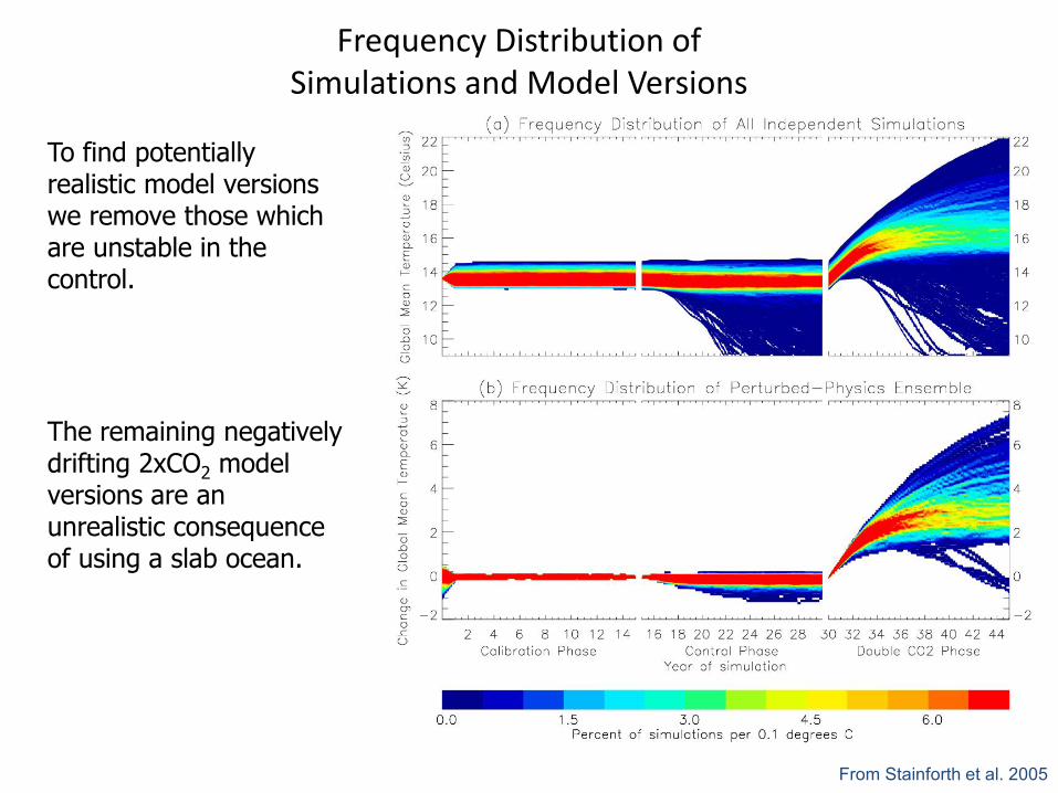
Frequency Distribution of Simulations and Model Versions

To find potentially realistic model versions we remove those which are unstable in the control. The remaining negatively drifting 2xCO2 model versions are an unrealistic consequence of using a slab ocean.



Frequency Distribution of Climate Sensitivity

Climate sensitivity is the equilibrium global mean surface temperature change in response to a doubling of atmospheric CO2 concentrations.

Sample model outcomes

Temperature Change Precipitation Change

Unperturbed model:

Model version with low climate sensitivity:

Model version with high climate sensitivity:

Regional Distributions (Later analysis: More simulations but similar to analysis in Phil Trans paper)

• 20,000 simulations • 6203 model versions with points

representing average over initial condition ensembles.

Interpreting perturbed physics ensembles (PPEs) {and multi-model ensembles (MMEs)}


Frequency Distribution of Climate Sensitivity No statement that this reflects probability of real world

behaviour

Lack of independence: The model versions are not independent samples of versions of this model let alone of the space of all possible models (whatever that might mean).



Parameter dependency of frequency distribution of climate sensitivity

Blue: No perturbations to entrainment coefficient

Red: No perturbations to cloud to rain conversion threshold


To the extent that any simulations are a plausible future, they all are:

“Domain of possibility” “Non-discountable envelope” “Lower bound on the maximum range of uncertainty”

Can the independence issues be solved by greater sampling of parameter space? A: No

• The shape of a model’s parameter space is arbitrary. It can depend on choices made by programmers to optimise the speed of the simulation.

• There is no objective or relevant subjective prior.

P1 Low High Stnd

Stnd

Low

High P2

Choice of parameter definition

Can we rule out certain model versions and reduce the uncertainty?

The “in-sample” problem A Conflict of Physics and Statistics

In-Sample Analysis: • Out-of-sample data can not be obtained in the

future. • Once published, further analysis becomes

biased. • Physicists tend to look at the extreme

behaviour but that process can’t be used to restrict the statistical inference.

Stainforth et al., 2005

Low Entrainment Coefficent: Rodwell & Palmer, 2007. Joshi et al., 2011

Setting aside the in-sample issue can we cull or down-weight some model versions?

When is a model too bad to be considered informative?

CMIP-2 coupled models

Single perturbations

Original model

All models are fundamentally different to reality what’s the basis for saying some are better than others as predictive tools?

Setting aside the in-sample issue can we cull or down-weight some model versions?

When is a model too bad to be considered informative?

CMIP-2 coupled models

Single perturbations

Original model

All models are fundamentally different to reality what’s the basis for saying some are better than others as predictive tools?

Murphy et al., 2004

None of this undermines the physical basis for expecting increasing greenhouse gases to lead to increasing

temperatures and severe climate disruption

Indeed one might argue it provides additional supporting evidence.

• It only undermines the quantitative interpretation of the details of complicated global climate model output.

What are we left with?

Due to: • Lack of independence. • Fundamental difference

between the model and reality.

• Misleading consequences of in-sample analysis.

“Domain of possibility” “Non-discountable envelope” “Lower bound on the maximum range of uncertainty”

Going forward

We should design ensembles to try to push out the bounds of the envelope. (Increase uncertainty?) Finding that we can not “push” models to produce certain responses can perhaps suggest (provide evidence for) constraints on how the real world system can respond. Note: This is counter to most funding calls which often seek for efforts to reduce uncertainty.

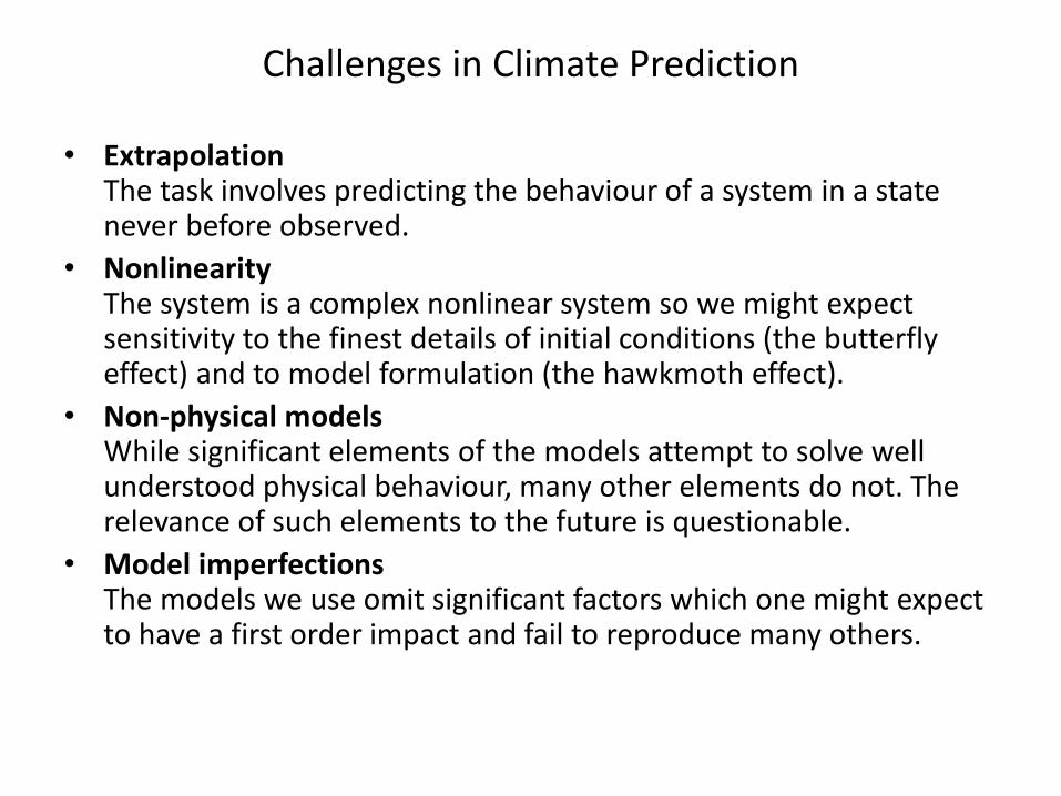
Challenges in Climate Prediction

• Extrapolation The task involves predicting the behaviour of a system in a state never before observed.

• Nonlinearity The system is a complex nonlinear system so we might expect sensitivity to the finest details of initial conditions (the butterfly effect) and to model formulation (the hawkmoth effect).

• Non-physical models While significant elements of the models attempt to solve well understood physical behaviour, many other elements do not. The relevance of such elements to the future is questionable.

• Model imperfections The models we use omit significant factors which one might expect to have a first order impact and fail to reproduce many others.

The Logistic Map and the Hawkmoth Effect

Model: Nt+1 = 4 Nt(1- Nt) System: Nt+1 =

−−+−− )1(

54)1()1(4 2

tttt NNNN εε

Laplace’s Demon and Climate Change, Frigg et al., 2013

Nt

Nt+

1

A Good Looking Model, Not A Good Forecasting System

Laplace’s Demon and Climate Change, Frigg et al., 2013

Timestep: 8

Timestep: 1 Timestep: 2

Timestep: 4

Comments and Questions

Questions, Debate, Arguments References

• Stainforth, D. A., Allen, M. R., Tredger, E. R. & Smith, L. A. Confidence, uncertainty and

decision-support relevance in climate predictions. Philos. Trans. R. Soc. A-Math. Phys. Eng. Sci. 365, 2145-2161

• Stainforth et al. Issues in the interpretation of climate model ensembles to inform decisions. Phil Trans Roy Soc. 365 (1857), 2163 (2007).

• Stainforth DA, Aina T, Christensen C, Collins M, Faull N, Frame DJ, et al. Uncertainty in predictions of the climate response to rising levels of greenhouse gases. Nature. 2005;433(7024):403-6.

• Frigg, R., L.A. Smith, D. A. Stainforth, The Myopia of Imperfect Climate Models: The Case of UKCP09, Philosophy of Science, 2013.

• Frigg, R., L.A. Smith, D. A. Stainforth, “An assessment of the foundational assumptions in high-resolution climate projections: the case of UKCP09”, Synthese, 2015.

Papers available from: [email protected]

mailto:[email protected]

Documents

The Interpretation Of Physically Based Climate Models ... · PDF fileThe Interpretation Of Physically Based Climate Models: Statistics .vs. Physics .vs. Philosophy D A Stainforth1,2