Embed Size (px)
Citation preview

The international monetary and financial system: A capital account historical perspective1
Claudio Borio
Harold James
Hyun Song Shin
This draft: 27 April 2014
1 Paper prepared for the Norges Bank conference, June 5-6, 2014

Abstract
In analysing the performance of the international monetary and financial system (IMFS), too much attention has been paid to the current account and far too little to the capital account. This is true of both formal analytical models and historical narratives. This approach may be reasonable when financial markets are highly segmented. But it is badly inadequate when they are closely integrated, as they have been most of the time since at least the second half of the 19th century. Zeroing on the capital account shifts the focus from the goods markets to asset markets and balance sheets. Seen through this lens, the IMFS looks quite different. Its main weakness is its propensity to amplify financial surges and collapses that generate costly financial crises – its “excess financial elasticity”. And assessing the vulnerabilities it hides requires going beyond the residence/non-resident distinction that underpins the balance of payments to look at the consolidated balance sheets of the decision units that straddle national borders, be these banks or non-financial companies. We illustrate these points by revisiting two defining historical phases in which financial meltdowns figured prominently, the interwar years and the more recent Great Financial Crisis.
JEL Classification: E40, E43, E44, E50, E52, F30, F40.
Keywords: excess financial elasticity, banking glut, current account, capital account, financial cycle, financial crises.

Contents
Introduction ............................................................................................................................................... 1
I. Analytical reference points ............................................................................................................. 3
The excess financial elasticity hypothesis ..................................................................................... 4
Measuring capital flows: which boundary? .................................................................................... 7
II. Interwar experience ...................................................................................................................... 10
III. The Great Financial Crisis ............................................................................................................ 24
Conclusion .............................................................................................................................................. 31

1
“When during the liquidity crisis of 1931 one European market after the other sustained sweeping withdrawals of short-term balances, the dangers involved in superabundance of international short-term lending became strikingly apparent. It was then felt that measures might have been taken to moderate the increasing indebtedness if the stupendous growth of liabilities had been known at the time.” 4th BIS Annual Report, 1934.
Introduction2
There is one history of the international monetary and financial system (IMFS) that is about
current accounts. It is the most popular and influential. It goes back to at least David Hume’s
view of the gold specie standard (Hume (1898)). It sees the economic havoc in the interwar
years through the eyes of the transfer problem (Keynes (1929a,b) and Ohlin (1929a,b)). It
identifies a systematic contractionary bias in the global economy because of an asymmetric
adjustment problem: deficit countries are forced to retrench while surplus countries are under
no pressure to expand (Keynes (1941)). It traces the 1970s woes and Latin American crisis
to the recycling of oil exporters’ surpluses (Lomax (1986), Congdon (1988)). It argues that a
saving glut, reflected in large Asian current account surpluses, was at the root of the Great
Financial Crisis that erupted in 2007 (Bernanke (2005, 2009), Krugman (2009), King (2010)).
And it is front and centre in G20 discussions, heavily preoccupied with global imbalances – a
short-hand for current account imbalances.
There is a parallel history that is about capital accounts. It is less popular and, in large part,
still to be written. It highlights the role of the mobility of financial capital in the gold standard
(Bloomfield (1959), De Cecco (1974)). It sees the economic turmoil of the interwar years
through the lens of large cross-border flows (Schuker (1988)). It focuses on biases and
asymmetries that arise from countries’ playing the role of bankers to the world (Triffin (1960),
Kindleberger (1965), Despres et al (1966)). It argues that a financial surge, unrelated to
current accounts, was at the origin of the Great Financial Crisis (Borio and Disyatat (2011),
Shin (2012)). It laments the peripheral attention that the G20 pay to financial, as opposed to
current account, imbalances. 2 I would like to thank Ben Cohen, Bob McCauley and Andreas Schrimpf for helpful comments and suggestions and Bilyana
Bogdanova and Michela Scatigna for excellent statistical support. The views expressed are my own and not necessarily those of the BIS.

2
Of course, these two views should be reconcilable. After all, the current and capital accounts
are part of the same balance-of-payments identity. And our sharp distinction between the two
histories is intentionally stylised. At times narratives diverge, but at others they intersect or
even merge (eg, Obstfeld (2010, 2012)).
That said, the lens matters. It matters for the analysis. To focus on current accounts means
zeroing in on the good markets – on output and expenditures – as well as on net capital
flows. To focus on the capital account means zeroing in on asset markets as well as on
gross capital flows and the corresponding stocks. In fact, most international finance macro
models nowadays are about current accounts and net flows, as the residual to consumption
and investment decisions. And the lens matters also for policy. Central banks have far less
influence on the current account than on the capital account: monetary and financial stability
policies – what central banking is all about -- are fundamentally about changes in asset
prices, portfolios and balance sheet positions.
This paper fits in this second, parallel history of the IMFS. Its premise is that in a highly
globalised economy financial markets hold sway and the most serious macroeconomic
problems arise from financial system breakdowns – systemic financial crises. These cannot
be understood by focusing on current accounts alone. In fact, in some important respects,
current accounts may be a distraction. The Achilles heel of the IMFS is not so much a
contractionary bias that reflects an asymmetric current account adjustment problem, what
might be termed a propensity to generate “excess saving”; rather, it is its propensity to
amplify the financial booms and busts – financial cycles -- that generate crises, what might
be termed its “excess financial elasticity” (Borio and Disyatat (2011), Borio (2014a)). Surges
and collapses in credit expansion, be these through banks – “banking gluts” – or securities
markets, are key ingredients (Shin (2012, 2013)), typically alongside equivalent surges and
collapses in asset prices, especially property prices (Drehmann et al (2012)).
Moreover, once we focus on the system’s excess financial elasticity we need to look beyond
the capital account. For one, the decision-making units, be these financial or non-financial,

3
often straddle borders. The residence principle that defines the boundary for the national
accounts, and hence also for the balance of payments, is inadequate: we need to consider
the consolidated income and balance sheet positions of the relevant players. In addition, the
currencies underpinning financial and real transactions, in which goods and services are
invoiced and, above all, assets are denominated, are often used outside national boundaries.
Some currencies play a huge role in the IMFS, most notably the US dollar – a point fully
understood by those steeped into international monetary system issues, but often overlooked
in standard macroeconomic models used to examine spillovers and coordination questions.
Finally, it is not so much the international component of the balance sheet position of a
country that matters, but how it fits into the overall balance sheet of the economy. Financial
and macroeconomic vulnerabilities can be properly assessed only in that context.
In this paper we illustrate these points by examining two historical phases of special interest:
the interwar years and the period surrounding the recent Great Financial Crisis. Both phases
featured high financial market integration globally and hence illustrate perfectly our
arguments.
The rest of the paper is organised as follows. Section I lays out the main analytical reference
points; it does so briefly, as they have been discussed in more detail elsewhere. Section II
revisits the interwar years, while Section III recalls the more recent experience.
I. Analytical reference points
Two analytical reference points anchor our discussion: the excess financial elasticity
hypothesis and the inadequacy of the national accounts boundary to capture the complex
web of financial transactions that can give rise to serious macroeconomic vulnerabilities.
Consider each in turn.

4
The excess financial elasticity hypothesis
Financial crises are not like meteorite strikes from outer space. They resemble volcanic
eruptions or earthquakes: they reflect the sudden and violent release of pressure that has
built up gradually over time. The pressure takes the form of protracted financial booms,
which often straddling business cycle fluctuations until they become unsustainable, thereby
sowing the seeds of their subsequent demise. The build-up of such financial imbalances
gives rise to endogenous boom-bust processes, or “financial cycles” (Borio (2013)). Systemic
banking crises typically occur towards their peak and usher in the bust phase; the
subsequent recessions are especially deep and the recoveries weak (eg, Drehmann et al
(2012a)).
The most characteristic hallmark of these cycles is the surge and collapse in credit
expansion (eg, Drehmann et al (2011), Haldane et al (2011), Jordá et al (2011a), Drehmann
and Tsatsaronis (2014)), typically alongside equivalent fluctuations in asset prices, especially
property prices (Drehmann et al (2012)). And because as credit expansion proceeds retail
funding lags behind, a growing share of the financing comes from wholesale funding, such as
non-core bank deposits, often from international sources (Borio and Lowe (2004), Shin and
Shin (2011), Hahm et al (2013), Borio et al (2011)).
We do not have a full understanding of the forces at work. But a key mechanism involves the
self-reinforcing interaction between loosely anchored perceptions of value and risk as well as
attitudes towards risk, on the one hand, and liquidity or financing constraints, on the other. In
modern terminology, the “price of risk” moves highly procyclically, amplifying financial and
economic fluctuations (eg, Borio et al (2001), Danielsson et al (2004), Adrian and Shin
(2010)). It is this interaction that imparts considerable inertia to the process.
Borio and Disyatat (2011) and Borio (2014) use the term “excess financial elasticity” to
denote the property of an economic system that generates the build-up of financial
imbalances. They focus, in particular, on the inability of the financial and monetary regimes

5
to constrain those imbalances. Think of an elastic band that stretches out further but, at
some point, inevitably snaps back. So used, the term “elasticity” takes root way back in the
history of economic thought, when it denoted the elasticity of credit (eg, Jevons (1875)).
Financial and monetary regimes matter greatly. Liberalised financial systems weaken
financing constraints, thereby providing more room for the build-up of financial imbalances.
Indeed, the link between financial liberalisations and subsequent credit and asset price
booms is well documented. 3 And so do monetary policy regimes that do not directly respond
to that build-up. This was true for the gold standard, in which central banks kept interest rates
relatively stable unless the external or internal convertibility constraints came under threat.
And it is also true of regimes focused on near-term inflation control: the authorities have no
incentive to tighten policy as long as inflation remains low and stable. It is no coincidence
that the build-up of financial imbalances is all the more likely following major positive supply-
side developments (Drehmann et al (2012)): these put downward pressure on inflation while
at the same time providing fertile ground for financial booms, as they justify the initial
optimistic expectations – a source of what Kindleberger (2000) called the initial
“displacement”.
What is the role of the IMFS in all this? The IMFS can amplify the excess elasticity of
domestic policy regimes (Borio (2014)) through their interaction internationally.
Financial regimes interact. For one, mobile financial capital across currencies and borders
adds an important external (marginal) source of finance – hence the outsize role of external
credit in unsustainable credit booms (eg, Avdjiev et al (2012)). And when exchange rates are
flexible, it can induce overshooting in exchange rates, through familiar channels (eg,
Gyntelberg and Shrimpf (2011), Burnside et al (2012), Menkhoff et al (2012)). In fact, these
channels are analogous to those that result in unsustainable asset price booms in a domestic
context. More generally, in an integrated financial world risk perceptions and attitudes spread
across assets classes through the forces of arbitrage and become embodied in risk premia. 3 In the postwar period, the link first became evident following the experience of liberalisation in the Southern Cone countries
of Latin America in the 1970s (eg, Diaz-Alejandro (1985), Baliño (1987)).

6
This explains, for instance, why proxies for the global price of risk, such as the popular VIX
index, are closely correlated with global pricing of assets as well as capital and credit flows
(Forbes and Warnock (2012), Rey (2013)) – what Rey has termed the “global financial
cycle”.
And also monetary regimes interact. They can spread easy monetary conditions from core
economies to the rest of the world, thereby increasing the risk of unsustainable financial
imbalances. They do so directly, whenever currency areas extend beyond national
jurisdictions. Think, in particular, of the huge international role of the US dollar. Policy in
international-currency countries has a more direct influence on financial conditions
elsewhere. More importantly, they do so indirectly. If exchange rates are fixed, such as under
the gold standard, the transmission is immediate. But even when they are flexible, the
transmission can take place through resistance to exchange rate appreciation, ie through the
interplay of policy reaction functions (eg, McKinnon (1993)).4 Policymakers in the rest of the
world keep policy rates lower than otherwise and/or intervene and accumulate foreign
currency reserves. For instance, there is ample evidence that since the early 2000s at least
EMEs and advanced small open economies have kept interest rates below what traditional
benchmarks for purely domestic conditions would suggest (Hofmann and Bogdanova (2012))
and that the US federal funds rate helps to explain these deviations (Taylor (2013), Gray
(2013), Spencer (2013) and Takats (2014)).
This explains the choice of the two episodes examined in this paper. Both relate to historical
phases in which financial markets have been highly integrated and in which monetary
regimes have paid little attention to the build-up of financial imbalances, regardless of the
exchange rate regime. The rationale is consistent with the similar financial and economic
fluctuations that punctuated also the classical gold standard, especially in the periphery,
including Norway (eg, Goodhart and De Largy (1999), Gerdrup (2003)).
4 For a discussion of the limited insulation properties of exchange rate flexibility, see Borio et al (2011) and for a formalisation
of some of these channels, see Bruno and Shin (2013).

7
Measuring capital flows: which boundary?
Once the focus is on financial instability and its macroeconomic costs, current accounts fade
into the distance.
This is true from a behavioural standpoint. To be sure, large current account deficits may well
increase the costs of systemic banking crises. And, by definition, they reflect a situation in
which domestic demand far exceeds domestic output – a possible symptom of unsustainable
expansions. But, historically, some of the most disruptive banking crises have erupted in the
wake of financial booms that took hold in countries with large current account surpluses.5
Think of Japan in the 1980s-early 1990s and, as we will discuss below, the United States in
the 1920s. Moreover, as we write, a major financial boom has been underway for several
years in China.6
Equally, current accounts fade into the distance from a measurement or accounting
perspective (Borio and Disyatat (2011)). By construction, current accounts and the net capital
flows they represent reveal little about financing. They capture changes in net claims on a
country arising from trade in real goods and services and hence net resource flows. But they
exclude the underlying changes in gross flows and their contributions to existing stocks -- all
the transactions involving only trade in financial assets, which make up the bulk of cross-
border financial activity. As such, current accounts tell us little about the role a country plays
in international borrowing, lending and financial intermediation, about the degree to which its
real investments are financed from abroad, and about the impact of cross-border capital
flows on domestic financial conditions. They are effectively silent about the intermediation
patterns that trigger banking distress. 7
5 See also Jordá et al (2011b) and Gourinchas and Obstfeld (2012), who find a strong link between credit growth and banking
crises, but little link between these and current account positions. 6 For a development of this argument, and also a critique of the view linking current account surpluses to a saving glut and low
real interest rates, see Borio and Disyatat (2011). 7 Borio and Disyatat (2011) argue that the misleading focus on current accounts reflects the failure to distinguish sufficiently
clearly between saving and financing. Saving, as defined in the national accounts, is simply income (output) not consumed; financing, a cash-flow concept, is access to purchasing power in the form of an accepted settlement medium (money), including through borrowing. Investment, and expenditures more generally, require financing, not saving. Financial crises

8
Moreover, even gross capital flows and the corresponding stocks tell only part of the story.
To see this, and the more pervasive distortions that well-meaning simple analytical devices
can have in our thinking, it is worth stepping back and consider national income accounting
101.
The measurement of capital flows is traditionally based on the boundaries established by
national income accounting. The purpose of the national income boundary is to measure
aggregate output within a well-defined boundary of an “economic territory”. The
measurement rests on the residence principle. An economic entity (a firm, say) is deemed to
be resident in the economic territory if it conducts its principal economic activity within its
boundaries. The national income accounts further classify the activity into sectors and
subsectors according to the nature of the activity.
The boundary of the economic territory for national income accounting often coincides with
the national border, but need not do so. The principle of measurement is based on residence,
rather than nationality. So, even if a firm is headquartered elsewhere, as long as the firm
conducts its business within the boundary, it is counted as part of the aggregate activity of
the territory concerned.8
In the benchmark international finance macroeconomic models, the boundary defined in
national income accounting also serves two other roles, as it conveniently permits
aggregating all actors within the boundary.
First, the national income boundary is often taken to define the decision-making unit. Thus,
the residents within the boundary are aggregated into a representative individual whose
behaviour is deemed to follow an aggregate consumption function. In particular, the balance
sheet of the decision-making unit is defined by the boundary set by national income
accounting. The balance of payments and capital flows are defined by reference to the
reflect disruptions in financing channels, in borrowing and lending patterns, about which saving and investment flows are largely silent.
8 The recent working paper of the Irving Fisher Committee (BIS (2012)) gives an introduction to the conceptual distinctions in measurement of international financial positions.

9
increases in assets and liabilities of those inside the boundary against those outside. Since
the models typically further assume that assets and liabilities are perfect substitutes, they
end up considering only net capital flows, ie current accounts. Thus, capital inflows are
defined as the increase in the liabilities of residents to non-residents, where the
measurement is taken in net terms, as the change in assets minus that in liabilities. The
assumption of a representative agent makes this restriction even more natural.
Second, in simple economic models, the national income boundary is also assumed to define
the currency area associated with a particular currency. As a result, the real exchange rate
between two national income territories is defined as the ratio of the prices between the two
economic territories. The nominal exchange rate, in turn, is defined as the price of one
currency relative to another. Thus, implicitly, monetary policy by the central bank within the
boundary affects the residents within the boundary itself in the first instance. To the extent
that monetary policy has spillover effects, they may be captured either through the current
account and trade balances, or through capital inflows and outflows measured in residence
terms.
To recap, the boundary of an “economic territory” in international economics serves three
roles. First, it is the boundary relevant for national income accounting. Second, it is the
boundary that defines the decision-making unit, including its balance sheet. Third, it is the
boundary that distinguishes domestic currency from foreign currency.
The triple coincidence between the three roles of the national income boundary is a
convention followed in simplified economic models. It is not a logical consequence of the
measurement of output or of the underlying financial transactions. It probably reflects the fact
that these models were formulated and refined in an era when capital flows were not as
central as they have become subsequently, and the simplification has served a useful
purpose. That said, the triple coincidence between the three notions of economic boundaries
was a reasonable approximation only in a relative brief phase in the immediate post-war
period.

10
The reason is simple. For one, decision-making units straddle national boundaries. In a world
in which firms increasingly operate in multiple jurisdictions, consolidated income and balance
sheet data are more informative. For, it is these units that decide where to operate, what
goods and services to produce at what prices, and how to manage risks. Importantly, it is
these units that ultimately come under strain. Nationality, which reflects the consolidated
balance sheet of firms, rather than residence, often sets the more relevant boundary.9 Indeed,
the BIS consolidated banking statistics were created in the 1970s precisely to address this
shortcoming (Borio and Toniolo (2008), McGuire and Wooldridge (2005)). In addition, as
noted, international currencies are actively used well beyond the boundary of the currency
jurisdiction10. And the intersection between the nationality of the players and the currencies
they use is what matters most to understand currency and funding exposures, vulnerabilities
and the dynamics of financial distress.
With these analytical reference points in mind, it is now time to consider in more detail the
experience in the interwar years and around the Great Financial crisis.
II. Interwar experience
In the interwar story, the current account imbalance gives only a partial picture. While the
German current account deficit and the US surplus attracted an enormous amount of
attention at the time and since, the financial flows and the round-tripping between Germany
and its neutral neighbours, the Netherlands and Switzerland, were largely beneath the radar
screen for public policy. Their implications only became clear after a major financial crisis in
1931, in which foreign short term credits in Germany were frozen. Foreign borrowing by the
German private and public sectors occurred in foreign currencies, with dollar denominated
bonds and credits from the United States and sterling denominated bonds and credits from
9 “Nationality” in this context generally relates to the country where the company is headquartered. There may be different
criteria to decide to which country to assign a decision-making unit, but the principle of consolidation is not affected by this. 10 For instance, McCauley, McGuire and Sushko (2014) report that more than 80% of the dollar bank loans to borrowers
resident outside the United States were booked outside the United States.

11
the United Kingdom. German agents also accumulated foreign currency claims in other
countries, above all in the small neutral neighbours, and these sums then were relent to
German corporations. In the lead-up to the financial crisis, as German capital flight
accelerated, it was financed in part by drawing on credit lines of US and UK banks. As a
result, in 1931, there were net gold inflows to France, Switzerland and the Netherlands (of
$771 m.), and gold outflows from Germany but also from the United States and the United
Kingdom (Allen and Moessner (2012)). A schematic version of the 1920s flows is given
below:
Figure 2: The geography of capital flows in the interwar years
It is in the 1920s that the phenomenon of excess financial elasticity appeared in its modern
form. Although in the classical (pre-1914) gold standard regime financial instability was a
feature of many countries on the periphery – including the United States - the core countries
US Households US
Banks
German borrowers
Bonds Short term credits
Swiss banks sss
Swiss affiliates
border
border
Short term
credits FDI/portfolio
No net movement
Large net movement

12
of the gold standard, Great Britain, France, and also Germany, were comparatively stable
and after 1873 did not experience systemic crises. That relative stability was admired by the
National Monetary Commission in the U.S. after the panic of 1907, attributed to differing
European institutional arrangements, and held to be a reason for instituting a European-style
central bank (Mitchell (1911)).
The contrast between the generally modest prewar fluctuations at the core and the postwar
emergence of an outsize cycle is dramatically evident from comparative data on bank loans.
Before the war, bank loans relative to GDP grew gradually in all countries (Graph 1); and
even the sharp crisis of 1907 provided only a brief interruption to the trend. By contrast,
some, but not all, countries experienced very substantial bank gluts (or excess financial
elasticity) in the 1920s, with a collapse in the Great Depression. There is little sign of such a
glut in France or Great Britain, but the cycle is very noticeable in the Austrian, German and
American cases, and also in the Netherlands and in Switzerland (which is not included in the
Taylor/Schularick dataset).
The data on long term bank lending for fourteen countries collected by Taylor and
Schularick was used to test the relationship between expansion of bank lending in the pre-
Great Depression period (1924-1929) and output declines in the Great Depression (1929-
1932). There is a significant difference between the treated group (larger than median GDP
declines) and control (smaller than median GDP declines). Those countries with a large
decline in GDP during 1929-1932 had a larger increase in loans before 1929. The severity of
the Great Depression as measured conventionally by output, industrial production or
unemployment was thus significantly greater in the countries with the gluts. In the view of
Accominotti and Eichengreen (2013) the flows were chiefly driven by the outsize cycle in the
principal exporting country, the United States.
The gluts were linked through capital flows, but it is important to note that they were
not necessarily correlated with current account positions. The United States, with a
substantial surplus, and Germany, with a substantial deficit, both saw large credit and

13
property price booms (Graph 2).11 By contrast, France, with a large surplus, and Britain, with
trade deficits, did not experience the phenomenon (same Graph). Germany and the U.S.
were linked by a substantial gross capital flow, both in the form of bond issues and in bank
lending. Financial fragility played a major role in the build-up of vulnerability, and then in the
propagation of crisis.
The choice of currency regime alone does not explain the interwar pattern. France and
Great Britain returned to the gold standard, the former at a rate conventionally thought to be
undervalued and the latter at an overvalued rate as policymakers sought to restore the pre-
1914 parity. Banks in both countries engaged in international lending, and some of the
relatively small London merchant banks were heavily engaged in South America and Central
Europe, and consequently faced illiquidity or even insolvency threats in the Great Depression
(Accominotti (2014)). But the segmentation of British banking into merchant banks and
clearing banks meant that there was no general glut, and no generalized banking crisis after
the Central European collapse in the summer of 1931. Thus attempts to explain interwar
weakness primarily in terms of the gold standard and its constraints (Temin (1989),
Eichengreen (1992), Eichengreen and Temin (2010)) build on the argument about
asymmetric adjustment (Keynes (1940)); but they miss a central element in the vulnerability
of the interwar IMFS.
A key distinction between the pre-1914 world and that of the restored gold standard or gold
exchange standard in the 1920s was the centrality of bond financing before the First World
War, in contrast with the rise of bank credit afterwards. The most common explanation of the
1920s peculiarity lies in the preoccupation with normalisation, a return to peacetime normality.
With normality, there was an expectation that bond yields would fall. Consequently, short-
term bank financing was regarded as an attractive way of bridging the interim before the
normalisation, and the return of lower yields and thus less expensive financing. In addition,
the increased prominence of bank credit was driven by the financial reconstruction of
11 For a more detailed discussion of the credit boom in the United States, see (eg, Persons (1930), Robbins (1934),
Eichengreen and Mitchener (2003)).

14
European countries (especially in Central Europe) after wartime and postwar inflation and
hyper-inflation. The promise of a restoration of prewar conditions was the ground for the
initial optimism or “displacement”, in Kindleberger’s terminology, that generated the flows
which pushed the banking glut.
Graph 1: Bank loans relative to GDP 1896-1913 (from Taylor/Schularick dataset)
Graph 2: Bank loans relative to GDP 1924-1938 (from Taylor/Schularick dataset)
0
0,2
0,4
0,6
0,8
1
1,2
1896
1897
1898
1899
1900
1901
1902
1903
1904
1905
1906
1907
1908
1909
1910
1911
1912
1913
France
Germany
Netherlands
UK
US
0
0,1
0,2
0,3
0,4
0,5
0,6
0,7
0,8
1924
1925
1926
1927
1928
1929
1930
1931
1932
1933
1934
1935
1936
1937
1938
France
Germany
Netherlands
UK
US

15
The principal creditor country, the United States, experienced considerable financial
innovation, with a new market for foreign bonds developing as a supplement to the older
market for domestic bonds (Flandreau et al (2009)). In addition, while the traditional issuing
houses (notably J.P. Morgan) were very cautious about the burgeoning European market,
new, innovative and pushy houses such as the Boston bank Lee Higginson saw an
opportunity to win market share. Graph 3 provides some examples of the expansion of the
balance sheet and the assets of large internationally active US banks. By contrast, there was
much less innovation in the creditor countries that did not experience the glut.
Graph 3: U.S. Bank Leverage
0
2
4
6
8
10
12
14
-
500 000 000,00
1 000 000 000,00
1 500 000 000,00
2 000 000 000,00
2 500 000 000,00
3 000 000 000,00
1922192319241926192719281929193019311932
Chase National Bank Leverage Total Assets
PrimaryCapital:Capital,Surplus,UndividedProfitsTotalAssets/TotalCapital
16
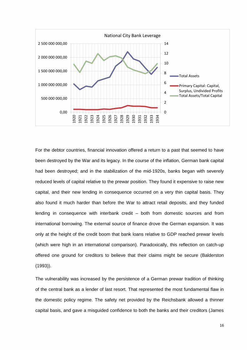
For the debtor countries, financial innovation offered a return to a past that seemed to have
been destroyed by the War and its legacy. In the course of the inflation, German bank capital
had been destroyed; and in the stabilization of the mid-1920s, banks began with severely
reduced levels of capital relative to the prewar position. They found it expensive to raise new
capital, and their new lending in consequence occurred on a very thin capital basis. They
also found it much harder than before the War to attract retail deposits, and they funded
lending in consequence with interbank credit – both from domestic sources and from
international borrowing. The external source of finance drove the German expansion. It was
only at the height of the credit boom that bank loans relative to GDP reached prewar levels
(which were high in an international comparison). Paradoxically, this reflection on catch-up
offered one ground for creditors to believe that their claims might be secure (Balderston
(1993)).
The vulnerability was increased by the persistence of a German prewar tradition of thinking
of the central bank as a lender of last resort. That represented the most fundamental flaw in
the domestic policy regime. The safety net provided by the Reichsbank allowed a thinner
capital basis, and gave a misguided confidence to both the banks and their creditors (James
0
2
4
6
8
10
12
14
0,00
500 000 000,00
1 000 000 000,00
1 500 000 000,00
2 000 000 000,00
2 500 000 000,00
1920
1921
1922
1923
1924
1925
1926
1927
1928
1929
1930
1931
1932
1933
1934
National City Bank Leverage
Total Assets
Primary Capital: Capital,Surplus, Undivided ProfitsTotal Assets/Total Capital

17
(1998)). While the banks appeared to have no liquidity constraints, the central bank in the
post-stabilisation world after 1924 was constrained by the convertibility requirements of the
gold standard.
The expansion of borrowing by Central European banks occurred in an informational or
statistical fog (BIS (1932, 1934)). While the extent of bond financing was quite well known,
because bond issues were managed publicly, the extent of foreign borrowing was not
appreciated. The bimonthly and then monthly bank balance sheets, whose publication was
required by law in Germany, do not distinguish between foreign and domestic liabilities:
although they do give figures for different terms or duration of borrowing. The Reichsbank’s
assessment of the size of short-term debt in early 1931 on the eve of the crisis was thus one
quarter lower than it should have been (Schuker (1988, p 57). It was only after the reversal of
flows, and the inability to make foreign exchange payments after the summer of 1931, that
the extent of the commercial short-term bank indebtedness became known, and statistical
overviews could be prepared. The initial assessment of the extent of Germany’s short-term
debt was presented in August 1931 by the Wiggin-Layton committee (Wiggin (1931)); but the
estimates rose further in the course of the following months (Special Advisory Committee
(1931)).
While the government banking and regulatory authorities knew about the phenomenon, they
were thus ignorant of its extent. The ignorance casts some doubt on a theory that explains
the large expansion of international credit in terms of a well-defined and deliberate strategy
on the part of the borrowers. It has been suggested that reparations debtors (and above all
Germany) tried to build up their foreign debt liabilities in order to engineer a payments crisis
in which the claims of reparations creditors and commercial and bank creditors would come
into conflict. According to this logic, when the debt level approached the point of
unsustainability, a crisis would be triggered in which the commercial creditors would assert
the priority of their claims, and in consequence press for the cancellation or radical reduction
of the reparation burden (Ritschl (2002)). The argument was laid out in the following way:

18
“Schacht [the President of the German central bank] appeared to be letting German banks
run up their short-term liabilities to correspondent institutions in Britain and American so that
the latter, fearing for their own liquidity, would entreat their governments to go easy in the
next reparations round.” (Schuker (1988), p 46)
This argument was certainly accepted by some of the lenders, and became a way of
boosting creditor confidence. A politically well-connected British banker, Reginald McKenna
of the Midland bank, made the observation that “under pressure of circumstances when
political and commercial forces are in the exchange market with marks to get foreign
currencies [to service debt], in practice the commercial would always get priority and success
and leave the political in the lurch. […] Each bank will act as a clearing house of marks
against sterling for its own customer. Each trade operation sets in motion its own demand
and offer of one of the two currencies. There would be a private arrangement within the walls
of the bank to clear these against each other before the balance of demand was released to
the open exchange market.” (Johnson (1978), pp 307-308)
The international flow of capital followed a complex web of linkages, often through decision
units that straddled borders. The tangled connections of Germany, a major borrower in the
1920s, and its immediate neighbors, the Netherlands and Switzerland, provide a powerful
illustration. Especially in the immediate aftermath of the First World War, many German
companies, including banks as well as non-financial corporations, acquired stakes, or formed
close relations with, banks in the Netherlands and Switzerland. There was an initial outflow of
funds in building these external relationships. The Dutch and Swiss companies were then
used as vehicles to borrow money, which was relent to Germany, often to the parent
company. International credit could be leveraged up in a foreign country, and the resulting
capital inflow could in turn be leveraged up in the recipient country. Within Germany, a
substantial discussion of the phenomenon of capital flight began even while U.S. money was
still flooding into Germany (James (1986)).

19
The motivation for the development of the outward flow from Germany was complex.
Originally, one reason may have been tax advantages from buying a foreign subsidiary and
running substantial operations through it. Initially, many of the fiscal advantages were
related simply to saving stamp duty and stock exchange taxes in Germany. A second
reason was that the wartime neutrality of the Netherlands and Switzerland meant that
companies there had been used to camouflage German ownership during the First World
War. But in the 1920s, a third reason was probably the decisive one: borrowing through a
non-German corporation substantially reduced the cost of credit, as a carry trade developed
with interest rates in the US and in the neutrals substantially lower than in Germany.
One of the best known examples of this sort of operation was the financial company IG
Chemie (Internationale Gesellschaft für Chemische Unternehmungen AG), incorporated in
Basel in 1928 under the control of the giant German chemical company IG Farben. One
year later, in 1929, after a capital increase to CHF 290 million, IG Chemie became one of the
largest Swiss corporations. Its explicit purpose was to build up international acquisitions for
the parent company, above all in Norway and the US as well as in Switzerland itself. The
Swiss driver of the business was an “IG Consortium” run by a small Swiss private bank,
Eduard Greuter, whose principal had already been working with one of the predecessor
companies of IG Farben, the Metallgesellschaft, before the First World War, operating a
company named “Metallwerte” that was a sort of predecessor of IG Chemie.
After the War, Greuter’s business consisted almost entirely in providing money for Germany.
In 1929 the Greuter bank borrowed from IG Farben in order to launch IG Chemie: the
German company provided about 70 percent of the funds. A small part of the capital came
from the large Swiss banks, which supplied much more extensive credit to IG Farben.
Representatives of the two largest Swiss banks sat on the board of the new company, where
they were given by unusually high compensation (four times that of board members for the
big Swiss banks). The Neue Zürcher Zeitung commented in the summer of 1929: “The
complicated and opaque construction of the Basel holding company can only be understood

20
in terms of the need for capital by the Frankfurt firm, which cannot itself raise capital directly.”
(König (2001)). For the German authorities, the main goal seemed to be reduction of IG
Farben’s tax liability, but a Finance Ministry note concluded that “such transactions cannot be
stopped if the mobility of international capital is not interfered with.” (James (1986), p 299).
In 1930 the Polyphonwerke concluded a similar transaction, as did the synthetic textile
company Vereinigte Glanzstof-Fabriken AG. So too did a state owned company, the
Prussian electricity works.
The circular character of some of this lending is obvious. Direct lending to German industrial,
commercial or agricultural business from Switzerland and the Netherlands amounted to no
less than 45 and 67 percent, respectively, on July 28, 1931, when the credits were frozen,
while for the US these direct loans represented a much smaller proportion, 28 percent. The
prominence of Switzerland and the Netherlands as intermediaries is revealed by the
calculation that corporations and individuals in these countries held 32.2 percent of
Germany’s short-term debt and 29.2 percent of the long-term debt (Statistisches Reichsamt,
(1932), Schuker (1988), p 117).
The rundown during the financial crisis in German banks and in Swiss banks occurred in
parallel. There was substantial capital flight, as the economic situation worsened and as the
fragile political stability of Germany was eroded. Such operations involved repaying German
loans from Swiss banks; German banks also saw their deposits fall and, in addition,
liquidated some of their foreign holdings. By the time the banking crisis hit in July 1931, the
Wiggin-Layton Committee’s estimate was that the short-term foreign assets of German
banks had contracted by 40 percent. Swiss bank claims against other banks contracted by a
similar amount, 52 percent, over the course of 1931 (Graph 4).
Graph 4: Swiss Bank Assets 1906-1938

21
The movements of funds out of Germany occurred well before the major U.S. banks started
to cut credit lines. It was only on June 23, 1931, for instance that the Bankers Trust
Company cut the credit line of Deutsche Bank. On July 6, only a week before the failure of a
large German bank, the Guaranty Trust Company announced immediate withdrawals.
These outside banks, unlike the insiders involved in the intricate German-Netherlands-
Switzerland loop, were relatively ill-informed, and also probably reluctant to trigger a panic in
which they were bound to lose their a substantial part of their assets.
There has been a considerable controversy about the extent to which the German banking
crisis was a banking crisis or a general currency and political crisis set off by the German
government’s desperate reparations appeal of June 6, 1931. The latter case is made by
Ferguson and Temin (2003). However, a look at the positions of individual banks suggests
that the withdrawals were not made equally from all German banks; those with a weak
reputation suffered the most dramatic outflows (Schnabel (2004); see also James (1984)).
Thus the Darmstädter- und Nationalbank (Danat), the bank with the most vulnerable
reputation, suffered an almost complete collapse of the bulk of its short term deposits
(between 7 days and 3 months maturity); there was also a run on the more solid Deutsche
Bank und Disconto Gesellschaft, but of a significantly less complete character (Graph 5).
0
1000
2000
3000
4000
5000
6000
7000
1906
1908
1910
1912
1914
1916
1918
1920
1922
1924
1926
1928
1930
1932
1934
1936
1938
Other Banks
Current Account
Other Advances

22
Graph 5: German Bank Deposits 1931 (Source: Die Bank)
Withdrawals from banks meant that the banks demanded more discounting facilities at the
central bank; but the Reichsbank refused because it was under pressure from the Bank of
England and the Federal Reserve Bank of New York to restrict its credit in order to stem the
developing run on the German currency. The central bank no longer had the currency
reserves it would have needed in order to satisfy the demand for foreign currency that arose
0
500
1000
1500
2000
2500
3000
in M
illio
ns o
f RM
Darmstaedter
Darmstaedter <7daysDarmstaedter 9days-3 moDarmstaedter >3moDarmstaedter BankDeposits
0,00
1000,00
2000,00
3000,00
4000,00
5000,00
6000,00
mar.28 mar.29 mar.30 mar.31 mar.32
in M
illio
ns o
f RM
Deutsche-Disconto
Deutsche-Disconto<7 days
Deutsche-Disconto 7days-3 mo
Deutsche-Disconto>3 mo
Deutsche-DiscontoBank Deposits
Deutsche-DiscontoTotal Liabilities

23
in the course of credit withdrawal. The Reichsbank no longer had operational freedom, but
was tied under the gold exchange standard system into a network of agreements, and
dependent on the willingness of other central banks to engage in swaps or other forms of
support.
In short, the fragility that had built up in the banking glut was a major cause of the reversal of
confidence, and of the major financial crisis that hit central Europe in the summer of 1931.
Ostensibly, excess financial elasticity was at work.

24
III. The Great Financial Crisis
We can trace similar forces behind the recent Great Financial Crisis. As is well known, the
crisis in the United States was preceded by a major financial boom. Credit and property
prices surged for several years against the backdrop of strong financial innovation and an
accommodative monetary policy.
Graph 6 Credit booms and external credit: selected countries
Thailand in the 1990s United Kingdom United States
In billions of US dollars
Thailand in the 1990s United Kingdom United States
Year-on-year growth, in per cent
The vertical lines indicate crisis episodes end-July 1997 for Thailand and end-Q2 2007 and end-Q3 2008 for the United States and the United Kingdom. For details on the construction of the various credit components, see Borio et al (2011). 1 Estimate of credit to the private non-financial sector granted by banks from offices located outside the country. 2 Estimate of credit as in footnote (1) plus cross-border borrowing by banks located in the country. 3 Estimate as in footnote (2) minus credit to non-residents granted by banks located in the country.
Source: Borio et al (2011).
By comparison with other credit booms, much of the credit expansion was financed from
purely domestic sources. As Graph 6 suggests, in keeping with the usual pattern, external
credit (blue lines and shaded areas) did outpace purely domestic ones (red line). But the

25
fraction of external funding as measured by the balance of payment statistics was low
compared to, say, the credit booms in Spain or the United Kingdom roughly at the same time.
Even so, this aggregate picture conceals the key role that foreign banks, especially
European Banks, and cross border flows more generally played in this episode. Indeed, the
subprime crisis illustrates well the importance of drawing the correct boundary for analysis for
capital flow analysis. In particular, European global banks sustained the shadow banking
system in the United States by drawing on dollar funding in the wholesale market to lend to
US residents through the purchase of securitised claims on US borrowers (Shin (2012)).
Figure 2: European banks in the US shadow banking system (Source: Shin (2012))
Figure 2 is a schematic that illustrates the direction of flows. It shows that European global
banks intermediate US Dollar funds in the United States by drawing on wholesale dollar
funding (for instance, from money market funds in the United States) which are then
reinvested in the securities ultimately backed by mortgage assets in the United States.
Capital first flows out of the United States and then flows back in. In this way, the cross-
border flows generated by the European global banks net out, and are not reflected as
imbalances in the current account.
US Households
USBorrowers
US Banking Sector
EuropeanGlobal Banks
border
Wholesalefunding market
Shadow bankingsystem

26
In the run-up to the crisis, money market funds in the United States played the role of the
base of the shadow banking system, in which wholesale funding is recycled to US borrowers
via the balance sheet capacity of banks, especially European banks.
Graph 7: Amount owed by banks to US prime money market funds (% of total), by
nationality of borrowing bank (Source: IMF GFSR October 2011; data from Fitch)
Graph 7, taken from the IMF’s Global Financial Stability Report of September 2011,
quantifies their role. It shows the amount that banks, classified by nationality, owed US prime
money market funds based on the top 10 by size, representing US$755 billion of
approximately US$1.66 trillion total prime money market fund assets. As a rule of thumb, 80%
of the money market fund assets were the obligations of banks and 50% of European banks.
The netting of gross flows shown in the schematic in Figure 2 is reflected in the items that
make up the US gross capital flows by category. Graph 8, taken from Shin (2012), shows the
categories of capital flows for the United States from the annual data published by the US
Bureau of Economic Analysis. Positive quantities (and bars) indicate gross capital inflows
0
10
20
30
40
50
60
70
80
90
2006 H2
2007 H1
2007 H2
2008 H1
2008 H2
2009 H1
2009 H2
2010 H1
2010 H2
2011 H1(%)
Asia
United States
Other Europe
Other euro area
Belgium, Italy,Spain, Portugal,Ireland, Greece

27
(the increase in claims of foreigners on the United States), while negative quantities indicate
gross capital outflows (the increase in the claims of US residents on foreigners).
Graph 8: U.S. annual capital flows by category (Source: Shin (2012), data from U.S.
Bureau of Economic Analysis.)
The grey shaded bars indicate the increase in claims of official creditors on the United States.
This includes the increase in claims of China and other countries accumulating foreign
exchange reserves. While official flows are large, private sector gross flows are larger still.
The negative bars before 2008 indicate large outflows of capital from the US (principally
through the banking sector), which then re-enter the country through the purchases of non-
Treasury securities.
The schematic of the “round-trip” capital flows through the European banks in Figure 2 is
useful in interpreting gross flows. European banks’ US branches and subsidiaries drove the
gross capital outflows through the banking sector by raising wholesale funding from US
money market funds and then shipping it to headquarters. Under the residence principle in

28
the national income and balance of payment accounts, foreign banks' branches and
subsidiaries in the United States are treated as US banks in the balance of payments, as the
balance-of-payments accounts are based on residence, not nationality.
The gross capital flows into the United States in the form of lending by European banks via
the shadow banking system no doubt played a pivotal role in influencing credit conditions
there in the run-up to the subprime crisis. However, since the Eurozone had a roughly
balanced current account while the United Kingdom was actually a deficit country, their
collective current account positions (net capital flows) vis-à-vis the US did not reflect the
influence of their banks in setting overall credit conditions in the country.
Moreover, the episode illustrates clearly the interaction between the nationality of the banks
and the foreign currency in which they operated. Policymakers at the time were caught
completely by surprise by the US dollar funding squeeze on European institutions. Why was
their need for US Dollars so large? The account above provides an explanation. More
generally, the BIS international banking statistics reveal that combined US dollar assets of
European banks reached some $8 trillion in 2008, including retail and corporate lending as
well as holdings of US securities – Treasury, agency and structured products (Borio and
Disyatat (2011)). Of this amount, between $300 and $600 billion was financed through
foreign exchange swaps, mostly short-term, against the pound sterling, euro and Swiss franc.
Estimates indicate that the maturity mismatch ranged between $1.1 to as high as $6.5 trillion
(McGuire and Von Peter (2009)). Hence the surprising funding squeeze that hit these banks’
(and others’) US dollar positions, and the associated serious disruptions in foreign exchange
swap markets – the so-called US dollar shortage (Baba and Packer (2008)). US money
market funds played a key role. In particular, the Lehman Brothers failure stressed global
interbank and foreign exchange markets because it led to a run on money market funds, the
largest suppliers of dollar funding to non-US banks, which in turn strained the banks’ funding
(Baba et al (2008), (2009)). The role of the US dollar as the currency that underpins the
global banking system is undiminished. In a recent paper, McCauley, McGuire and Sushko

29
(2014) report that more than 80% of the dollar bank loans to borrowers resident outside the
United States have been booked outside the United States.
To sum up, the role of European banks during the U.S. subprime mortgage crisis illustrates
well the importance of drawing the right boundary in international finance. Capital flows are
traditionally viewed as the financial counterpart to savings and investment decisions, in line
with the narrative of capital flowing “downhill” from capital-rich countries with lower rates of
return to capital-poor countries with higher returns (eg, Lucas (1990)). From this perspective,
the focus is typically on net capital flows, since that is what counts for funding a country’s
borrowing requirements. However, in the case of European banks intermediating US dollar
funding, the boundary defined for national income accounting is traversed twice, so that the
usual net flows do not capture the activities of the financial intermediaries engaging in the
maturity transformation in the mortgage market. And the institutions’ consolidated balance
sheet, covering also their operations in the United States, provides valuable additional
information. If the objective is to gauge credit conditions and overall financial vulnerability,
the current account was of very limited use. Rather than the global savings glut, a more
plausible culprit for subprime lending in the United States was the “global banking glut”.
The shortcomings of the often assumed “triple coincidence” between the national income
boundary, decision-making balance sheet and the currency area have again become evident
since then (Shin (2013)). In this case, the symptom has been the rapid pace of bond
issuance by emerging market borrowers in offshore locations since 2010. And, once again,
this is happening as several of their counties of origin have been experiencing strong
financial booms ((Caruana (2014), Borio (2014a)). The amount outstanding of international
debt securities of private sector borrowers has displayed a yawning gap between the total
measured by the nationality of the borrower (based on the location of the headquarters of the
borrower) and the total by residence. As of the end of 2013, outstanding international debt
securities of private sector borrowers from emerging economies stood at 0.97 trillion dollars

30
by residence of issuer and 1.73 trillion dollars by nationality of issuer, implying a gap of $758
billion.12
Moreover, the currency composition of offshore corporate bond issuance by emerging
market firms has been tilted toward the US dollar (McCauley, Upper and Villar (2013)). As a
result, emerging market borrowers have become sensitive to US dollar funding conditions
and interest rates even though they may be remote from the United States geographically.
If the proceeds of the borrowing are sent to headquarters through an explicit capital account
transaction, the balance of payments accounts would show a capital inflow in the form of
greater external liabilities of the headquarters to its overseas subsidiary. Misleadingly, this
may be recorded as FDI. However, if the multinational firm chooses to classify the
transaction as part of trade flows in goods and services - for instance through the practice of
"over-invoicing" where the value of exports are inflated - then the traditional balance of
payments account would not capture the flow as an increase in the liabilities of the
headquarter’ s unit.
Figure 3: Offshore borrowing by multinational corporation
12 http://www.bis.org/statistics/secstats.htm
Multinationalcorporation
AA L
L
Internationalcapital market
US dollars
Border
Localcurrency
A L
Bank
Localcurrency
Localcurrency

31
Figure 3 also illustrates the impact of such transactions on the domestic financial system of
the recipient economy if the proceeds are held as short-term financial claims in local
currency. On a consolidated basis, the multinational firm has a currency mismatch on its
balance sheet, with dollar liabilities in its overseas subsidiary and local currency assets at
headquarters. One motivation for such a currency mismatch may be to hedge currency risk
on cash flow denominated in US dollars, but another motivation would be the speculative one
of positioning the company's balance sheet to benefit from the appreciation of the local
currency against the dollar. In practice, hedging and speculation may be difficult to
distinguish, even ex post. Whatever the motivation, the local currency financial assets held
by the firm will then be on-lent by intermediaries thereby impacting the overall financial
conditions in the local economy (Shin (2013), Turner (2014)).
Conclusion
As we have learnt once more in the wake of the Great Financial Crisis, finance and
macroeconomics are inextricably linked. And what is true domestically is also true
internationally. In the current historical phase, both real and financial markets are highly
integrated globally, just as they were almost uninterruptedly for many decades until the Great
Depression. The need to develop new analytical frameworks to think about the interaction
between finance and macroeconomics in a domestic context inevitably extends to the global
stage.
This calls for a reversal in the prevailing perspective. One should not ask what the real side
of the equation means for its financial counterpart, but what the financial side means for its
real counterpart. The starting point should be what happens in financial asset markets rather
than in the goods markets, domestically and internationally. Otherwise, there is a risk that the
financial side will be neglected. This is precisely what has happened for far too long. There is
a need to redress the balance. Through the alternative lens, the world looks quite different.

32
In this paper we have taken some steps in this direction, focusing on the international
dimension. We have highlighted three points. First, in a financially integrated global
economy, the IMFS tends to amplify the “excess financial elasticity” of national economies,
raising the risk of financial crises with huge macroeconomic costs. Second, current accounts
are largely uninformative about these risks; the relevant information is contained in the
capital accounts and in their relationship to the broader balance sheets of the relevant
economies. Third, there is a need to go beyond the resident/non-resident distinction that
underpins the balance-of-payments and to consider the consolidated balance sheets of the
decision-making units that operate across borders, including the currencies of denomination.
Put differently, the single boundary that sets the “economic territory” in standard international
finance macroeconomic models, in which residence defines who produces and consumes, its
financial assets and liabilities and, often, the currency of denomination, is badly inadequate.
The experiences of the interwar years and of those surrounding the Great Financial Crisis
illustrate these points nicely. In both cases, financial surges and collapses within and across
national borders were at the root of the historic financial crises. Current account positions did
not provide a useful pointer: surges occurred in both surplus and deficit countries. And in
both cases, understanding the build-up of vulnerabilities requires looking beyond the capital
account to what decision-making units operating in multiple jurisdictions were doing – banks
and non-financial corporates in the interwar years, and, above all, the nexus between
European banks and US money market funds in the US sub-prime crisis. Moreover, since
then non-financial corporations in EMEs have been taking on substantial external debt that is
not captured by residence-based statistics – potentially another source of significant
vulnerability.
This analysis has major implications for central banks. Given their primary responsibility for
monetary and financial stability, central banks inevitably end up under the spotlight once the
focus shifts to asset prices, balance sheets and financial crises. As long as the focus is on
current accounts, central banks’ role is necessarily more peripheral. This is not the place to

33
expand on what all this means for policy (eg, Borio (2013b, 2014a,b), Caruana (2012a,b and
2014b)). There is little doubt, however, that policy frameworks should be strengthened to
incorporate more systematically financial surges and collapses. And in a highly globalised
world, ways should also be found to take proper account of policy spillovers, both on other
countries and on aggregate conditions.

34
References
Accominotti, O (2014): "London merchant banks, the Central European panic and the Sterling crisis of 1931", Journal of Economic History.
Accominotti, O and B Eichengreen (2013), “The mother of all sudden stops: capital flows and reversals in Europe, 1919-1932, CEPR Working Paper.
Avdjiev, S, R McCauley and P McGuire (2012): “Rapid credit growth and international credit: Challenges for Asia”, BIS Working Papers, no 377, April.
Baba, N, R McCauley and S Ramaswamy (2009): “US dollar money market funds and non-US banks”, BIS Quarterly Review, March, pp 65–81.
Baba, N and F Packer (2008): “Interpreting derivations from covered interest parity during thefinancial market turmoil of 2007–08”, BIS Working Papers, no 267, December.
Baba, N, F Packer and T Nagano (2008): “The spillover of money market turbulence to FXswap and cross-currency swap markets”, BIS Quarterly Review, March, pp 73–86.
Balderston, T (1993): The origins and course of the German economic crisis : November 1923 to May 1932, Berlin: Haude & Spener.
Baliño, T (1987): “The Argentine banking crisis of 1980”, IMF Working Papers, no WP/87/77.
Bank for International Settlements (BIS) (1932): 2nd BIS Annual Report, Basel.
______ (1934): 4th BIS Annual Report, Basel.
______ (2012) “Residency/local and nationality/global views of financial positions” IFC Working Paper no 8, Irving Fisher Committee on Central Bank Statistics, http://www.bis.org/ifc/publ/ifcwork08.htm
Bernanke, B (2005): “The global saving glut and the U.S. current account deficit,” the Sandridge Lecture, Richmond, March 10.
______ (2009): “Financial reform to address systemic risk,” Speech at the Council on Foreign Relations, Washington, D.C, 10 March.
Borio, C (2013a): “The financial cycle and macroeconomics: what have we learnt?”, Journal of Banking & Finance, in press. Also available as BIS Working Papers, no 395, December.
——— (2013b): “On time, stocks and flows: understanding the global macroeconomic challenges”, National Institute Economic Review, August. Slightly revised version of the lecture at the Munich Seminar series, CESIfo-Group and Süddeutsche Zeitung, 15 October, 2012, which is also available in BIS Speeches.
——— (2014a): “The Achilles heel of the international monetary system: what it is and what to do about it”, paper prepared for a keynote lecture at the Festschrift in honour of Niels Thygesen.
——— (2014b): “Monetary policy and financial stability: what role in prevention and recovery?”, BIS Working Papers no 440, February. Forthcoming in Capitalism and Society.
Borio, C and P Disyatat (2011): “Global imbalances and the financial crisis: link or no link?”, BIS Working Papers no 346, May. Revised and extended version of “Global imbalances and the financial crisis: Reassessing the role of international finance”, Asian Economic Policy Review, 5, 2010, pp 198-216.
Borio, C and P Lowe (2004): “Securing sustainable price stability: should credit come back from the wilderness?”, BIS Working Papers no 157, July.
Borio, C, R McCauley and P McGuire (2011): “Global credit and domestic credit booms” BIS Quarterly Review, September, pp 43-57.

35
Borio, C and G Toniolo (2008): “One hundred and thirty years of central bank cooperation: A BIS perspective” in C Borio, G Toniolo and P Clement (eds) The past and future of central bank cooperation, Studies in Macroeconomic History Series, Cambridge, UK: Cambridge University Press.
Bruno, V and H Shin (2013): “Capital flows and the risk-taking channel of monetary policy”, BIS Working Papers no 400, December.
Burnside, C, M Eichenbaum and S Rebelo (2011b): “Carry trade and momentum in currency markets”, Annual Review of Financial Economics, vol. 3, pp 511-35.
Caruana, J (2012): “International monetary policy interactions: challenges and prospects”, Speech at the CEMLA-SEACEN conference on "The role of central banks in macroeconomic and financial stability: the challenges in an uncertain and volatile world", Punta del Este, Uruguay, 16 November.
——— (2014a): “Global liquidity: where it stands, and why it matters”, IMFS Distinguished Lecture at the Goethe University, Frankfurt, Germany, 5 March.
——— (2014b):”Global economic and financial challenges: a tale of two views”, lecture at the Harvard Kennedy School in Cambridge, Massachusetts, 9 April.
Congdon, T (1988): The debt threat: The dangers of high real interest rates for the world economy, Oxford: Basil Blackwell.
Danielsson, J, H Shin and J Zigrand (2004): “The impact of risk regulation on price dynamics”, Journal of Banking and Finance, vol 28, pp 1069-87.
De Cecco, M (1974): Money and empire: the international gold standard, Oxford: Blackwell.
Despres, E, C Kindleberger and W Salant (1966): The dollar and world liquidity: a minority view, Brookings Institution, Washington D.C.
Diaz-Alejandro, C (1985): “Good-bye financial repression, hello financial crash”, Journal of Development Economics, vol 19, pp 1-24.
Drehmann, M, C Borio and K Tsatsaronis (2011): “Anchoring countercyclical capital buffers: the role of credit aggregates”, International Journal of Central Banking, vol 7(4), pp 189-239.
______ (2012): “Characterising the financial cycle: don’t lose sight of the medium term!”, BIS Working Papers, no 380, June.
Eichengreen, B (1992): Golden fetters: The gold standard and the great depression, 1919-39, Oxford: Oxford University Press.
Eichengreen, B and K Mitchener (2003): “The Great Depression as a credit boom gone wrong”, BIS Working Papers, no 137, September.
Eichengreen, B and P Temin (2010): "Fetters of gold and paper," Oxford Review of Economic Policy, vol 26(3), pp 370-384.
Ferguson, T and P Temin (2003): “Made in Germany: the German currency crisis of 1931,” Research in Economic History, 21, pp. 1–53.
Flandreau, M, Flores, Gaillard, Nieto-Parra (2009): "The end of gatekeeping: underwriters and the quality of sovereign bond markets, 1815-2007," NBER Working Paper no 15128.
Forbes, K and F Warnock (2012) "Capital flow waves: surges, stops, flight and retrenchment" Journal of International Economics, vol 88(2), pp 235-251
Goodhart, C and P De Largy (1999): “Financial crises: plus ça change, plus c’ est la même chose”, LSE Financial Markets Group Special Paper, no 108.
Gourinchas, P-O and M Obstfeld (2012): "Stories of the twentieth century for the twenty-first." American Economic Journal: Macroeconomics, 4(1): 226-65.

36
Gray, C (2013): “Responding to the monetary superpower: investigating the behavioural spillovers of US monetary policy”, Atlantic Economic Journal, vol 41(2), pp 173-84.
Gyntelberg, J, and A Schrimpf (2011): “FX strategies in period of distress.” BIS Quarterly Review, December, pp 29-40.
Hahm, J-H, H Shin and K Shin (2013): “Noncore bank liabilities and financial vulnerability”, Journal of Money, Credit and Banking, vol 45(1), pp 3-36.
Hofmann, B and B Bogdanova (2012)): “Taylor rules and monetary policy: a Global Great Deviation?”, BIS Quarterly Review, September, pp. 37-49.
James, H (1984): “The causes of the German banking crisis of 1931”, Economic History Review, vol 38, pp. 68–87.
______ (1986): The German slump: politics and economics 1924-1936, Oxford: Oxford University Press
______ (1996): International monetary cooperation since Bretton Woods, Washington DC and Oxford, IMF and Oxford University Press.
______ (1998): “Die Reichsbank 1876 bis 1945, in (ed.) Deutsche Bundesbank, Fünfzig Jahre Deutsche Mark: Notenbank und Währung in Deutschland seit 1948”, Munich: C.H. Beck, pp. 29-89.
______ (2001): The end of globalization: lessons from the Great Depression. Harvard: Harvard University Press.
Jevons, W (1875): Money and the mechanism of exchange, New York: D. Appleton and Co.
Johnson, E (1978): Collected writings of John Maynard Keynes XVIII, activities 1922-1932, the end of reparations, Cambridge 1978: Royal Economic Society.
Jordá, O, M Schularick and A Taylor (2011a): "When credit bites back: Leverage, business cycles and crises". Federal Reserve Bank of San Francisco Working Paper Series 2011-27.
Jordá, O, A Taylor and M Schularick (2011b): “Financial crises, credit booms, and external imbalances: 140 years of lessons”, IMF Economic Review, vol 59, pp 340-378.
Keynes, J (1929a): “The German transfer problem”, Economic Journal, vol 39, pp 1-7.
______ (1929b): “The reparations problem: a discussion. II. A rejoinder”, Economic Journal, vol 39, pp179-82.
______ (1941): “Post-war currency policy”, memoranda reproduced in D Moggridge (ed) (1980): The collected writings on John Maynard Keynes, vol 25, Activities 1940-1944, Shaping the post-war world: the Clearing Union, MacMillan/Cambridge University Press.
Kindleberger, C (1965): “Balance-of-payments deficits and the international market for liquidity”, Princeton Essays in International Finance, no 46, May.
______ (2000): Manias, panics and crashes, Cambridge: Cambridge University Press, 4th edition.
King, M (2010): Speech delivered to the University of Exeter Business Leaders’ Forum, 19 January.
König, (2001): Interhandel: Die schweizerische Holding der IG Farben und ihre Metamorphosen – eine Affäre um Eigentum und Interessen (1910–1999), Zurich: Chronos.
Krugman, P (2009): “Revenge of the glut,” The New York Times, 1 March.
Lomax, D (1986): “The developing country debt crisis”, London: Macmillan.
Lucas, R (1990): “Why doesn’t capital flow from rich to poor countries?” American Economic Review 80 (May), pp 92–96.

37
Ma, G and R McCauley (2013): “Global and euro imbalances: China and Germany”, BIS Working Papers, no 424, September. Forthcoming in M Balling and E Gnan (eds), 50 years of money and finance: Lessons and challenges, Vienna and Brussels: Larcier.
McCauley, R, P McGuire and V Sushko (2014): “Global dollar credit: links to US monetary policy and leverage” paper prepared for the 59th Panel Meeting of Economic Policy, April 2014.
McCauley, R, C Upper and A Villar (2013): “Emerging market debt securities issuance in offshore centres”, BIS Quarterly Review, September, pp 22–3.
McGuire, P and G von Peter (2009): “The US dollar shortage in global banking and the international policy response,” BIS Working Paper, no. 291, October.
McKinnon, R (1993): “The rules of the game: International money in historical perspective”, Journal of Economic Literature, vol 31(1), pp 1-44.
Menkhoff, L, L Sarno, M Schmeling, and A Schrimpf (2012): “Currency Momentum Strategies.” Journal of Financial Economics, vol 106(3), pp 660–84.
Mitchell, W C (1911): “The Publications of the National Monetary Commission,” Quarterly .
Obstfeld, M (2010): “Expanding gross asset positions and the international monetary system,” Remarks at the Federal Reserve Bank of Kansas City symposium on “Macroeconomic Challenges: The Decade Ahead,” Jackson Hole, Wyoming, August 26–28.
______ (2012): “Does the current account still matter?”, American Economic Review, 102(3), pp 1-23.
Ohlin, B (1929a): “The reparation problem: a discussion”, Economic Journal, vol 39, June, pp 172-183
______ (1929b): “Mr. Keynes’ views on the transfer problem. II. A Rejoinder from Professor Ohlin”, Economic Journal, vol 39, pp 400-4.
Persons, C (1930): “Credit expansion, 1920 to 1929, and its lessons”, Quarterly Journal of Economics, vol 45(1), pp 94-130.
Rey, H (2013): “Dilemma not trilemma: the global financial cycle and monetary policy independence”, paper presented at the Federal Reserve of Kansas City Economic Policy Symposium "Global Dimensions of Unconventional Monetary Policy", Jackson Hole, 22-24 August.
Ritschl, A (2002): Deutschlands Krise und Konjunktur 1924-1934 : Binnenkonjunktur, Auslandsverschuldung und Reparationsproblem zwischen Dawes-Plan und Transfersperre, Berlin : Akademie Verlag.
Robbins, L (1934): The Great Depression, New York: Macmillan.
Schnabel, I (2004): “The twin German crisis of 1931”, Journal of Economic History, vol 64, pp 822–871.
Schuker, S (1988): “American ‘reparations’ to Germans, 1919‐33: Implications for the Third World debt crisis”, Princeton Studies in International Finance, no. 61, July.
Shin, HS and K Shin (2010): “Procyclicality of monetary aggregates”, NBER Working Paper no 16836, February.
Shin, HS (2012): “Global banking glut and loan risk premium” Mundell‐Fleming Lecture, IMF Economic Review, vol 60(2), pp 155‐192.
______ (2013): “The second phase of global liquidity and its impact on emerging economies”, Keynote address at the Federal Reserve Bank of San Francisco Asia Economic Policy Conference, November 3-5.

38
Special Advisory Committee (1931): Report of the Special Advisory Committee, issued at Basle, 23 December.
Spencer, M (2013): “Updating Asian ‘Taylor rules’”, Deutsche Bank, Global Economic Perspectives, 28 March.
Statistisches Reichamt (1932): “Die deutsche Auslansverschuldung,” Wirtschaft und Statistik , August, pp 490-493.
Taylor, J (2013): “International monetary policy coordination and the great deviation, Journal of Policy Modelling, in press.
Takats, E (2014): “How does US monetary policy affect policy rates in emerging market economies?“, BIS Quarterly Review, March, pp 6-7.
Temin, P (1989): Lessons from the Great Depression, Cambridge: MIT Press.
Triffin, R (1960): Gold and the dollar crisis; the future of convertibility, Yale University Press: New Haven.
Turner, P. (2014): “The global long-term interest rate, financial risks and policy choices in EMEs” BIS Working Papers, no 441, February.
Wiggin, A (1931): Report of the Committee Appointed on the Recommendation of the London Conference 1931, Basel, August 18.