Embed Size (px)
Citation preview
The Influence of Volatile RawMaterial Prices on InventoryValuation and Product Costing
Logistiikka
Maisterin tutkinnon tutkielma
Hannu Suviolahti
2009
Liiketoiminnan teknologian laitos
HELSINGIN KAUPPAKORKEAKOULUHELSINKI SCHOOL OF ECONOMICS
HELSINGIN KAUPPAKORKEAKOULU Logistiikka
THE INFLUENCE OF VOLATILE RAW MATERIAL PRICES ON INVENTORY VALUATION AND PRODUCT COSTING
Pro gradu -tutkielma Hannu Suviolahti 6.3.2009
Hyväksytty liiketoiminnan teknologian laitoksella 6.3.2009 arvosanalla
_________________________________________________________
Tomi Seppälä Katri Karjalainen
i
Helsinki School of Economics Department of Business Technology Master’s thesis Hannu Suviolahti The Influence of Volatile Raw Material Prices on Inventory Valuation and
Product Costing
Abstract Efficient product costing and inventory valuation are much emphasized in today’s manufacturing environment because of their importance in management decisions. However, especially volatile raw material prices bring challenges to reliability of product costing and inventory valuation. This relatively little regarded, but important viewpoint is investigated in this research. The research problem is stated as follows: how should raw material flow around raw material inventory be valuated? In literature review eight factors that should be considered when choosing inventory valuation and product costing methods were determined. Based on these factors three variables that affect the efficiency of raw material inventory valuation and product costing were defined, and they were tax shield benefits, product costing accurateness and how well information reflects the performance of a company. For the empirical part a framework was formed based on these three variables. In the empirical part a simulation model was built and based on the model raw material inventory valuation methods were evaluated. A scenario analysis was done in order to analyze generality and robustness of raw material inventory valuation methods. Using the simulation model and the scenario analysis different raw material inventory valuation methods are evaluated in a real company environment, and results that cannot be derived analytically are disclosed. By using a correct raw material inventory valuation method business can be much improved. In the case company on which the simulation model is based, product costing error can be decreased by 14 % of product costs and inventory value fluctuation by 7 % of inventory value by just choosing adequate inventory valuation method. The main determinant of the magnitude in improvements is raw material price behavior. In the case of high inflation the benefits of using correct inventory valuation method can be very great. Also volatility of raw material prices affects results significantly. The main contribution of this research is the investigation of the effects of uncertain raw material prices in the context of product costing and inventory valuation. The main result that contradicts current research is that FIFO (first-in first-out) should not be used for raw material accounting. In general, LIFO (last-in last-out) and market prices are efficient raw material inventory valuation methods. Yet, the choice between these two depends on objectives of management accounting. However, it was observed that material flow behavior has no significant effect on the ranking of different raw material inventory valuation methods, and thus the main results can be generalized to different companies. Keywords: inventory valuation, product costing, raw material price, FIFO, LIFO, weighted average cost, market price Number of pages (including appendices): 117
ii
Helsingin kauppakorkeakoulu Liiketoiminnan teknologian laitos Pro gradu -tutkielma Hannu Suviolahti
Voimakkaasti vaihtelevien raaka-ainehintojen vaikutukset varastonarvostukseen ja tuotekustannuslaskentaan
Tiivistelmä
Tuotekustannuslaskenta- ja varastonarvostusmenetelmien merkitys korostuu etenkin nykyajan tuotantoympäristöissä, koska kyseiset menetelmät ovat tärkeitä johdon apuvälineitä. Kuitenkin voimakkaasti vaihtelevat raaka-ainehinnat madaltavat kustannuslaskennan ja varastonarvostuksen luotettavuutta. Tämä on tärkeä ja kirjallisuudessa vähälle huomiolle jäänyt aihe, ja siksi se on otettu tämän tutkimuksen kohteeksi. Tutkimusongelma tässä työssä voidaan lausua seuraavasti: kuinka raaka-ainemateriaalivirta raaka-ainevaraston ympärillä tulisi arvostaa? Kirjallisuuskatsauksessa löydettiin kahdeksan yleistä tekijää, jotka tulisi ottaa huomioon arvostusmenetelmien valinnassa. Näiden pohjalta määritettiin kolme raaka-aineiden arvostuksen hyvyyteen vaikuttavaa tekijää, jotka olivat tuotekustannuslaskennan tarkkuus, informaation oikeellisuus ja verosuojan hyödyt. Empiiristä osaa varten muodostettiin viitekehys edellä mainittujen kolmen tekijän pohjalta. Empiirisessä osassa rakennettiin simulointimalli, jonka perusteella arvioitiin yleisimpiä raaka-aineiden varastonarvostusmenetelmiä, joita olivat FIFO (first-in first-out), LIFO (last-in first-out), painotetun keskiarvon menetelmä, markkinahintamenetelmä ja kolmen kuukauden keskiarvo -menetelmä. Tutkimuksessa toteutettiin myös skenaarioanalyysi, jonka avulla arvioitiin tuloksien yleistettävyyttä sekä arvostusmenetelmien eri tilanteisiin sopeutuvuutta. Simulointien ja skenaarioanalyysin perusteella raaka-aineiden varastonarvostusmenetelmien toimivuutta arvioitiin oikeassa tuotantoympäristössä. Arvostusmenetelmien oikealla valinnalla yrityksen suorituskykyä voidaan selkeästi parantaa. Caseyrityksessä tuotekustannuslaskennan virhettä voidaan pienentää 14 %:lla tuotteen kustannuksista ja varastonarvon heilahtelua 7 %:lla varastonarvosta valitsemalla oikea varastonarvostusmenetelmä. Muuttuja, joka pääosin määrää parannuksien suuruuden, on raaka-ainehintojen käyttäytyminen. Korkean inflaation tapauksissa menetelmien erot toisiinsa nähden kasvavat merkittävästi. Myös raaka-ainehintojen heilahtelujen suuruudella on paljon merkitystä. Merkittävin tämän tutkimuksen lisä olemassa olevaan tutkimukseen on satunnaisesti muuttuvien raaka-ainehintojen vaikutusten arviointi tuotekustannuslaskennan ja varastonarvostuksen kontekstissa. Tärkein tulos, joka on ristiriidassa aiemman kirjallisuuden kanssa, on se, että FIFO-menetelmää ei tulisi käyttää raaka-ainevirtojen arvostukseen. Yleisesti parhaiten sopivat menetelmät ovat LIFO ja markkinahintamenetelmä, ja valinnan näiden kahden välillä tulisi perustua johdon laskentatoimen tavoitteisiin. Tutkimuksessa huomattiin, että raaka-ainevirran käyttäytyminen ei vaikuta merkittävästi raaka-ainevaraston arvostusmenetelmien keskinäiseen järjestykseen, ja siksi tutkimuksen päätulokset voidaan yleistää erilaisiin yritysympäristöihin. Asiasanat: varastonarvostus, tuotekustannuslaskenta, raaka-ainehinta, FIFO, LIFO, painotetun keskiarvon menetelmä, markkinahinta Sivujen lukumäärä (liitteineen): 117

iii
Acknowledgements
I want to extend my sincere thanks to Professor Tomi Seppälä and Ph.D student Katri
Karjalainen at Helsinki School of Economics (HSE) for all the support during my thesis. I am
indebted to them for excellent ideas and guiding from the problem definition to the finishing
touches of my thesis.
I grateful to my supervisor at Metos, Finance director Yvonne Malin-Hult, for giving me this
splendid opportunity to prepare master’s thesis in an extraordinary company on an interesting
subject. I want to thank her for all the support in the thesis making process. My special thanks
to Director Yrjö Sulavuori at Metos for interesting discussions and instructions and overall for
the whole Metos’ personnel for helpful attitude towards my project.
Helsinki, 6th of March
Hannu Suviolahti
iv
THE INFLUENCE OF VOLATILE RAW MATERIAL PRICES ON INVENTORY VALUATION AND PRODUCT COSTING
Abstract Tiivistelmä (Abstract in Finnish) Acknowledgements List of Figures List of Tables List of Symbols 1 Introduction ........................................................................................................... 1
1.1 Motivation .................................................................................................................. 1 1.2 Research Problem and Objectives .............................................................................. 3 1.3 Limitations ................................................................................................................. 4 1.4 Structure ..................................................................................................................... 4
2 Product Costing, Inventory Valuation and Price Fluctuation .......................... 6 2.1 Relevance of Inventory Valuation and Product Costing ............................................ 6
2.1.1 Introduction to Management Accounting .............................................................. 6 2.1.2 Product Costing Effects on Business ..................................................................... 7 2.1.3 Importance and Challenges of Valuing Raw Material Inventory .......................... 8
2.2 Modeling Raw Material Price Behavior ..................................................................... 9 2.2.1 Time-Series Forecasting Models .......................................................................... 10 2.2.2 Regression Analysis ............................................................................................. 14
2.3 Product Costing ........................................................................................................ 18 2.3.1 Different Aspects of Product Costing .................................................................. 18 2.3.2 Methods of Calculating Product Costs ................................................................. 21
2.4 Inventory Valuation Methods ................................................................................... 23 2.4.1 Specific identification .......................................................................................... 23 2.4.2 First-In First-Out .................................................................................................. 24 2.4.3 Last-In First-Out ................................................................................................... 25 2.4.4 Weighted Average Cost ....................................................................................... 26 2.4.5 Other Methods for Inventory Valuation ............................................................... 29 2.4.6 Comparison of Inventory Valuation Methods ...................................................... 30
3 Guidelines for Evaluating Raw Material Inventory Valuation and Product Costing ......................................................................................................................... 37
3.1 Research Framework ................................................................................................ 37 3.2 Case Company Introduction ..................................................................................... 39
3.2.1 Metos Finland Oy ................................................................................................. 39 3.2.2 Inventory Valuation and Product Costing at Metos Finland Oy .......................... 40
3.3 Evaluation Criteria of Inventory Valuation Methods ............................................... 41 3.4 Research Method of Empirical Study ...................................................................... 42
3.4.1 Quantitative Research Methods ........................................................................... 42
v
3.4.2 Simulation as a Research Method ........................................................................ 43 4 Simulation Model to Evaluate Inventory Valuation Methods ........................ 47
4.1 Data Used in Simulation Model ............................................................................... 47 4.2 Modeling Stainless Steel Prices ............................................................................... 48 4.3 Modeling Nickel Prices ............................................................................................ 51 4.4 Simulation of Material Flow .................................................................................... 56 4.5 Structure of Simulation Model ................................................................................. 60
5 Results of Simulations ......................................................................................... 66 5.1 Inventory Value Fluctuation Due to Stainless Steel Prices ...................................... 66 5.2 Product costing accurateness .................................................................................... 69 5.3 Eliminating Contradiction with Reported Inventory Value ..................................... 72 5.4 Profit from Tax Shield .............................................................................................. 75 5.5 Best Inventory Valuation Methods Based on Simulations ....................................... 79 5.6 Conclusions Based on Simulation Results ............................................................... 84 5.7 Scenario Analysis ..................................................................................................... 88
6 Conclusions .......................................................................................................... 95 6.1 Summary .................................................................................................................. 95 6.2 Integral Results ......................................................................................................... 97 6.3 Further Research ...................................................................................................... 99
References
vi
List of Figures
Figure 2-2 - Typical cost structure of a Finnish manufacturing unit (Lukka & Granlund 1994) .......................................................................................................................................... 20
Figure 3-1 - The framework of the research ............................................................................ 37 Figure 4-1 - “Nickel cash official fixing - ask” -index behavior from 4th of February 2000 .. 52 Figure 4-2 - A single simulation process with one inventory valuation method ..................... 61 Figure 4-3 - 20 random nickel price paths in simulations ........................................................ 62 Figure 4-4 - 20 random stainless steel price paths in simulations ............................................ 63 Figure 4-5 - Amount of production, purchases and inventory in one random path ................. 64 Figure 4-6 - Inventory value by different methods in one random path .................................. 65 Figure 5-1 - The distributions of IVF in the simulations (n=5000) with different methods .... 67 Figure 5-2 - The distributions of RIVF in the simulations (n=5000) with different methods . 68 Figure 5-3 - The distributions of PCA in simulations (n=5000) with different methods......... 70 Figure 5-4 - The distributions of RPCA in simulations (n=5000) with different methods ...... 71 Figure 5-5 - The distributions of DWAC in simulations (n=5000) with different methods .... 73 Figure 5-6 - The distributions of RDWAC in simulations (n=5000) with different methods . 74 Figure 5-7 - The distributions of TSP in simulations (n=5000) with different methods ......... 77 Figure 5-8 - Averages of TSPI with different rates of return with different inventory valuation
methods ............................................................................................................................ 79 Figure 5-9 - Averages of RIVF, RPCA and RDWAC in simulations ...................................... 85 Figure 5-10 - Improvements compared to 3-month average method in significant criterions
with different methods ..................................................................................................... 86 Figure 5-11 - Differences compared to WAC .......................................................................... 87 Figure 5-12 - Assumptions in scenario analysis ....................................................................... 89 Figure 5-13 - Average RIVF in different scenarios ................................................................. 90 Figure 5-14 - Average RPCA in different scenarios ................................................................ 91 Figure 5-15 - Average RDWAC in different scenarios ............................................................ 92 Figure 5-16 - Average TSPI in different scenarios .................................................................. 93
vii
List of Tables
Table 2-1 - Inventory accounting methods in the case of inflation (Financial education 2008) .......................................................................................................................................... 31
Table 2-2 - Factors determining the optimal inventory valuation policy ................................. 36 Table 4-1 - Correlation analysis: testing significance of correlations between independent
variables and stainless steel price ..................................................................................... 49 Table 4-2 - Correlation analysis: removing multicollinearity .................................................. 50 Table 4-3 - Regression analysis: Nickel price changes with lags 1, 2 and 3 months are
independent variables, stainless steel price change is dependent variable ....................... 51 Table 4-5 - AIC with different ARMA-models ....................................................................... 54 Table 4-6 - SBIC with different ARMA-models ..................................................................... 54 Table 4-7 - HQIC with different ARMA-models ..................................................................... 55 Table 4-8 - AIC, SBIC and HQIC with different ARCH-models ............................................ 56 Table 4-9 - Correlation analysis: correlations between purchases and production .................. 57 Table 5-1 - The average, standard deviation, standard error, minimum and maximum of IVF
in simulations (n=5000) with different methods .............................................................. 67 Table 5-2 - The average, standard deviation, standard error, minimum and maximum of RIVF
in simulations (n=5000) with different methods .............................................................. 69 Table 5-3 - The average, standard deviation, standard error, minimum and maximum of PCA
in simulations (n=5000) with different methods .............................................................. 70 Table 5-4 -The average, standard deviation, standard error, minimum and maximum of RPCA
in simulations (n=5000) with different methods .............................................................. 72 Table 5-5 - The average, standard deviation, standard error, minimum and maximum of
DWAC on a five-year interval in simulations (n=5000) with different methods ............ 73 Table 5-6 - The average, standard deviation, standard error, minimum and maximum of
RDWAC in simulations (n=5000) with different methods .............................................. 75 Table 5-7 - The average, standard deviation, standard error, minimum and maximum of TSP
in simulations (n=5000) with different methods .............................................................. 77 Table 5-8 - Average TSP and TSPI in simulations (n=5000) .................................................. 78 Table 5-9 - Average TSPI with different discount rates with different methods ..................... 79 Table 5-10 - Summary of the results of DWAC, IVF, PCA and TSPI .................................... 80 Table 5-11 - Summary of the results of RDWAC, RIVF, RPCA and TSPI ............................ 80 Table 5-12 - The best methods when RPCAP = 0 with different PRDWAC and PRIVF ................... 82
Table 5-13 - The best methods when RPCAP = 1500 with different PRDWAC and PRIVF ............. 82
Table 5-14 - The best methods when RPCAP = 3000 with different PRDWAC and PRIVF ............. 82
Table 5-15 - The best methods when RPCAP = 7500 with different PRDWAC and PRIVF ............. 82
Table 5-16 - The best methods in Finland when RPCAP = 0 with different PRDWAC and PRIVF .. 83
Table 5-17 - The best methods in Finland when RPCAP = 1500 with different PRDWAC and PRIVF
.......................................................................................................................................... 83

viii
Table 5-18 - The best methods in Finland when RPCAP = 3000 with different PRDWAC and PRIVF
.......................................................................................................................................... 83 Table 5-19 - The best methods in Finland when RPCAP = 7500 with different PRDWAC and PRIVF
.......................................................................................................................................... 84 Table 5-20 - The effect on relative performance of inventory valuation methods if price
volatility, price trend or material flow volatility increases .............................................. 94
ix
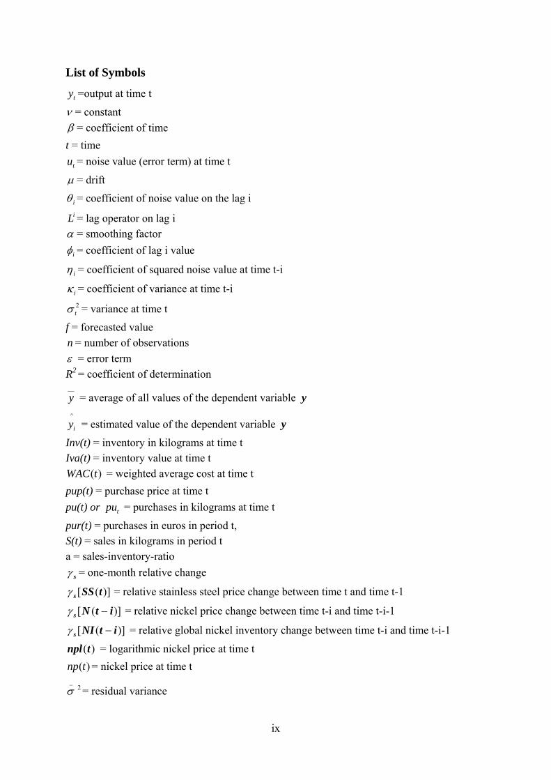
List of Symbols
ty =output at time t
ν = constant β = coefficient of time t = time
tu = noise value (error term) at time t
μ = drift
iθ = coefficient of noise value on the lag i iL = lag operator on lag i
α = smoothing factor
iφ = coefficient of lag i value
iη = coefficient of squared noise value at time t-i
iκ = coefficient of variance at time t-i 2tσ = variance at time t
f = forecasted value n = number of observations ε = error term R2 = coefficient of determination __
y = average of all values of the dependent variable y ^
iy = estimated value of the dependent variable y
Inv(t) = inventory in kilograms at time t Iva(t) = inventory value at time t
)(tWAC = weighted average cost at time t pup(t) = purchase price at time t pu(t) or tpu = purchases in kilograms at time t
pur(t) = purchases in euros in period t, S(t) = sales in kilograms in period t a = sales-inventory-ratio
sγ = one-month relative change
)]([ tSSsγ = relative stainless steel price change between time t and time t-1
)]([ itNs −γ = relative nickel price change between time t-i and time t-i-1
)]([ itNIs −γ = relative global nickel inventory change between time t-i and time t-i-1
)(tnpl = logarithmic nickel price at time t )(tnp = nickel price at time t
2_σ = residual variance
x
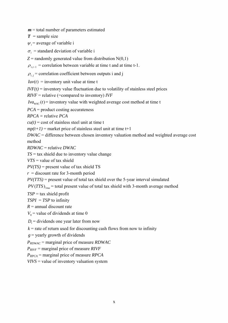
m = total number of parameters estimated T = sample size
iψ = average of variable i
iσ = standard deviation of variable i
Z = randomly generated value from distribution N(0,1)
1, −ttρ = correlation between variable at time t and at time t-1.
ji ,ρ = correlation coefficient between outputs i and j
)(tIuv = inventory unit value at time t IVF(t) = inventory value fluctuation due to volatility of stainless steel prices RIVF = relative (=compared to inventory) IVF
)(tIvaWAC = inventory value with weighted average cost method at time t
PCA = product costing accurateness RPCA = relative PCA cu(t) = cost of stainless steel unit at time t mp(t+1) = market price of stainless steel unit at time t+1 DWAC = difference between chosen inventory valuation method and weighted average cost method RDWAC = relative DWAC TS = tax shield due to inventory value change VTS = value of tax shield PV(TS) = present value of tax shield TS r = discount rate for 3-month period PV(TTS) = present value of total tax shield over the 5-year interval simulated
maTTSPV 3)( = total present value of total tax shield with 3-month average method
TSP = tax shield profit TSPI = TSP to infinity R = annual discount rate
0V = value of dividends at time 0
1D = dividends one year later from now k = rate of return used for discounting cash flows from now to infinity g = yearly growth of dividends PRDWAC = marginal price of measure RDWAC PRIVF = marginal price of measure RIVF PRPCA = marginal price of measure RPCA VIVS = value of inventory valuation system
1
1 Introduction Management accounting has grown in importance in organizations since the 20th century when its
effect on business performance became understood. The importance is straightforwardly derived:
what cannot be measured cannot be managed, and what cannot be managed cannot be improved.
If something cannot be measured, it is impossible to take correct actions. Nowadays competition
across businesses is tough and profit margins are small, so every decision is important. Thus
accurate management accounting information is extremely valuable. Choosing product lines,
harvesting or acquiring businesses, hiring or firing personnel are some examples of matters that
are heavily affected by management accounting information.
This research is about product costing and inventory valuation, which are essential areas in
management accounting. These two areas have their importance, for example, in product pricing
and profitability calculations. However, constantly changing and complex business environment
brings a lot of challenges to product costing and inventory valuation. In some industries the
number of products can be hundreds, thousands, or even tens of thousands. These products may
be situated at a number of warehouses. The products may also be manufactured from various raw
materials. Thus it is impossible for a manager to evaluate even the operations of his own
company without getting accurate information from products and inventories. To get more
accurate management accounting information, corporations have implemented various softwares.
Management accounting is also a major part, for example, in different ERP-softwares. However,
these softwares are very expensive, and thus the information must be acquired efficiently. So the
challenge of acquiring accurate information as cheaply as possible still remains. Thus there is
always need for management accounting research, especially in the area of product costing and
inventory valuation.
1.1 Motivation
There has been a continuing controversy over the best method of appreciating material flow,
especially in valuating inventory. There are many studies about choosing a correct inventory
valuation method between FIFO (first-in first-out) and LIFO (last-in first-out). Some famous
examples include Morse & Richardson (1983) and Dopuch & Pincus (1988). Many of these
2
studies investigate how firms should choose a correct method based on one or two factors. These
individual factors are important, but there is a need for research, which completely analyzes the
factors, their effects on each other and answers the foremost question of choosing the optimal
method taking all factors into consideration. This would be essential to companies, which are
searching for an optimal method for them. For companies, it is the overall situation that matters,
not the individual factors.
Another, but more important motivation to this research is that there exists no research that
considers the effects of volatile raw material price movements when choosing optimal inventory
valuation and product costing methods. There are studies that recommend LIFO under inflation
(such as Wilson & Walter 2003), but these studies do not consider the effects of volatility in raw
material prices. This is quite surprising, because raw material valuation is essential, especially in
the upstream of the supply chain.
Volatility of raw material price brings problems to valuation of inventory. When prices increase
or decrease substantially, inventory and material flow valuation follow a way behind. Then, for
example, product costing and thus pricing goes wrong and management accounting figures (such
as profit margin) cannot be trusted. Inventory valuation and product costing have also a straight
effect on cash flow. Biddle (1980) estimated that the 105 firms in his study paid an average of
nearly $26 million in additional federal income tax due to absence of optimal inventory valuation
methods. Thus, huge savings can be achieved by choosing the correct method. But as Bar-Yosef
& Sen (1992) conclude, when deciding an optimal accounting policy one must consider distortion
of information as well as tax gains achieved. Thus companies are faced with an important, but
challenging problem.
This research was motivated because of these two major gaps in current research, which were
absence of overall analysis of all factors and volatility in raw material prices. These two gaps
indicate that companies do not have guidelines for choosing the correct inventory valuation and
product costing methods under volatile raw materials. After this research, companies struggling
with fluctuating raw material prices should be able to analyze their situation a lot better than
currently. A company struggling with these problems was selected as a case company to this
research. The empirical study is based on the case company; in this way we are able to study the
effects of fluctuating raw material prices on business of a successful and experienced company.
3
1.2 Research Problem and Objectives
Based on the previous, inventory valuation has major direct and indirect effects on cash flows of
companies. The main direct effect is the effect on tax obligations. Inventory valuation and
product costing affect indirectly by distorting information, and the distorted information makes
difficult to make correct decisions. The focus of this research is to investigate inventory valuation
and product costing to improve these direct and indirect effects. In addition, volatile raw material
prices bring another challenge to appreciating inventory and the cost of products. Thus the
research problem is constructed around volatile raw material, and the main objective is to
discover the most efficient way to appreciate material flow around raw material inventory. So the
research problem of this investigation can be stated as follows: How should raw material flow
around raw material inventory be valuated?
First of all, in order to analyze product costing and inventory valuation under volatile raw
material prices, price behavior of the raw material needs to be analyzed. For this study a case
company was chosen, which is struggling with fluctuating stainless steel prices. These prices
have been especially volatile during latest years. Thus the first objective is to model stainless
steel price behavior.
After the behavior of the stainless steel price has been investigated, the main focus is on how the
raw material flow should be appreciated. Before choosing actual methods to value raw material
flow, the factors affecting ranking of valuation policies are considered. So the second objective is
to determine the factors affecting raw material inventory valuation and product costing policy.
After the factors are determined, next task is to value the actual raw material flow. Inflow of raw
material to inventory is clear, because it is valuated based on purchase prices. This is the only
possible way. Then the first thing is to value this raw material when it is in the inventory. Thus
the inventory valuation policy, that is the most efficient for companies, has to be investigated. So,
the third objective of this research is to find out the most efficient way to value raw material
inventory.
Finding the optimal way to value raw material inventory does not consider product costing. Flow
out from inventory should be appreciated efficiently, because product costing is based on this
4
appreciation. So the final objective is to discover the most efficient way to value raw material
flow out of inventory.
Therefore, the objectives described previously are shortly as follows:
1. To model stainless steel price behavior
2. To find out factors that determine the most efficient raw material inventory valuation and
product costing policy
3. To find out the most efficient way to value raw material inventory
4. To discover the most efficient way to value raw material flow out of inventory.
1.3 Limitations
When starting this research three major limitations were defined. First of all, this research
considers product costing and inventory valuation on behalf of raw material. Raw material
inventory here is limited from inbound to the boundary between company and its supplier. From
outbound the raw material inventory is limited to the boundary between raw material inventory
and production. That’s why no end-products or semi-finished products are taken into account.
Second major limitation is due to specific raw material. Raw material in the case company, and
thus in this research, is stainless steel. So, especially in the empirical part only stainless steel is
considered, and no other raw material is taken into account.
Third limitation is that the empirical part of this research is based on the case company’s
environment. Therefore, all company-specific inputs and overall environment is based on the
case company, and thus this research does not consider any other company.
1.4 Structure
This research is divided into two main parts: literature review and empirical research. First, in
chapter 2 a literature review is covered, which has four parts. In the first part relevance of
inventory valuation and product costing is considered, in the second part modeling of raw
material behavior is discussed, the third part includes a review of product costing and in the final
part inventory valuation methods are evaluated. Based on this literature review, a framework for
the empirical part is constructed. The framework is introduced and analyzed in chapter 3, as well
as the research methods used. The main aspect in the empirical part is formulation of the

5
simulation model around the research problem. The simulation model is introduced in chapter 4
and results of the simulations are analyzed in chapter 5. In the last chapter the whole research is
summed up and main conclusions are made.
6
2 Product Costing, Inventory Valuation and Price Fluctuation In this literature review inventory valuation, product costing and modeling of prices are covered.
This literature review is divided into four subsections. First, relevance of inventory valuation and
product costing for business are discussed in section 2.1. Then behavior and forecasting of raw
material prices are covered in 2.2. In the final two subsections first product costing is dealt
(section 2.3) and in the last section (2.4) inventory valuation is covered.
2.1 Relevance of Inventory Valuation and Product Costing
In this subchapter some basics of management accounting are covered first. After the
introduction to management accounting, significances of product costing and inventory valuation
are discussed.
2.1.1 Introduction to Management Accounting
Definitions of management accounting can be found in most textbooks, and one major
professional definition by Institute of Cost and Management Accountants is as follows: “the
application of professional knowledge and skill in the preparation and presentation of accounting
information in such a way as to assist management in the formulation of policies and in the
planning and control of the operations of the undertaking” (Fanning 1983, 2). Whatever the
definition is like, the basic objectives of management accounting, as Belkaoui (1980) highlights,
include (1) supplying information for internal decision makers, (2) facilitating their decision
making, (3) motivating their actions and behavior in a given direction and (4) promoting
efficiency of organization.
Nowadays in business there are many drivers that increase the need for efficient management
accounting. Especially contemporary economic environment demands excellence from corporate
management accounting systems. Time-based competition exists in almost all industries, which
stresses the importance of management accounting. Because of many reasons, including
fluctuations in raw material prices, organization’s management accounting system must provide
timely and accurate information to facilitate efforts to control costs, to measure and improve
productivity and to devise improved production processes (Johnson & Kaplan 1991, 3–4). If
7
there is an improper match between the accounting system and firm’s objectives, management
can make incorrect decisions and investments (Campbell 1995).
One vital area in management accounting is product costing. Product costing affects pricing,
inventory valuation and overall profit calculations heavily. That’s why the significance of product
costing is covered next.
2.1.2 Product Costing Effects on Business
Product costing has major implications in running a business. Because of its importance, product
costing has been researched a lot. Identifying cost drivers and developing activity-based costs is
important for managerial purposes such as pricing and evaluating profitability of products and
product lines (Dominiak & Louderback III 1994, 555). Keys, Balmer & Creswell (1987) argue
that product costing makes designers aware of product’s potential for production and indicates
potential cost reduction areas. Ostwald (1992) and Alnestig & Segerstedt (1996) argue that the
most important objective of product costing is determining appropriate sales prices. Profit margin
of the product is calculated based on product costs and sales price. Most profitable products are
chosen, and thus product costing has major implications for product mix. (Lea & Fredendall
2002)
However, the management accounting system often fails to provide accurate product cost
information. Costs are usually distributed by simplistic and arbitrary measures that do not
represent the use of company’s resources. This failure to provide accurate costs for individual
products may lead to misguided decisions about product pricing, product sourcing and product
mix. (Johnson & Kaplan 1991, 2) If calculated product cost is not correct, whenever company’s
total demand is greater than company’s production capacity, it is probable that product mix is not
optimal. Sometimes even unprofitable products are manufactured due to incorrect product costs.
(Lea & Fredendall 2002) By correctly choosing product costing system business performance can
be clearly improved (Reinstein & Bayou 1997).
Jianxin & Tseng (1999) raise important operational problems in product costing. These include
lack of accountants’ manufacturing excellence, dependence on detailed design description, lack
of structured mapping between design and production and contextual heterogeneity. These
problems are especially relevant in design phase. In the design phase the product structure can be
8
changed most easily, and thus it is very relevant that the product costing is evaluated starting
from the design, or even before that. (Jianxin & Tseng 1999)
Inventory valuation and product costing go hand in hand. Whenever changes in product costing
are made, the effect of the changes on inventory valuation has to be considered. This relation is
easily explained as follows: whenever product costs increase, inventory value decreases, and vice
versa. Because of this tight relationship, when product costing is discussed, inventory valuation
has to be covered too. The next chapter discusses importance of inventory valuation.
2.1.3 Importance and Challenges of Valuing Raw Material Inventory
Inventory is often the largest and most important asset that a company owns. As an asset,
inventory has a direct impact on profitability of the company and especially on reporting the
company’s success in the balance sheet. Inventories appear on the balance sheet and the income
statement under heading current assets. So, inventory valuation affects both the profitability and
committed capital of the company. In each accounting period appropriate expenses must be
matched with revenues in order to determine appropriate income. In inventory accounting this
includes determining cost of goods sold that should be deducted from sales. That’s why the net
income depends directly on inventory valuation. (Hermanson, Edwards, Maher 2005, 258) Based
on the direct effect on net income, inventory valuation affects cash flows. This is because taxes to
be paid depend on net income. Selection of inventory valuation policy can alter cash flows due to
tax obligations. (Bar-Yosef & Sen 1992)
Inventory accounting rules may also affect stockholders’ wealth, because managers who are paid
income-based can potentially distort inventory to maximize their payoffs. For example, if
managers are paid based on return-on-equity (ROE), minimizing committed capital (including
inventory) is profitable for these managers. Inventory value can be affected by the choice of
inventory valuation policy without altering operations. Thus stockholders, by directly or
indirectly dictating the accounting policy choice, can use accounting rules to implement their
preferences and control managers. (Bar-Yosef & Sen 1992)
A major challenge in inventory valuation is volatility of raw material price and because of this
volatility there are major differences between the inventory value and the budgeted value. That’s
why it is important to separate out total variance into planning variance and operational variance.
9
Planning variances seek to explain how original standards need to be adjusted in order to reflect
changes in operating conditions (e.g. raw material price changes) between current situation and
the time when the standard was originally calculated. In effect it means that the original standard
is updated so that it is a realistic target in current conditions. Operational variances indicate the
extent to which attainable targets (i.e. the adjusted standards) have been achieved. Operational
variances are thus a realistic way of assessing performance. (Lucey 2003, 262–263)
There are basically two general approaches to classify cost variances for controlling purposes.
First, there is an approach that classifies all variances as expenses. In this approach any savings
or expenses above or below normal are abnormal. If a management sees that for control purposes
inventory at cost of standard price reflects better the situation in the company, then it is
reasonable to classify variances as period expenses. Second, especially for financial reporting and
accounting purposes, there is an actual costing method. The variances in this method are prorated
to inventories and cost of sales. (Hirsch & Louderback 1986, 354–355) The most common
method to allocate variances in overhead costs is to assign those to cost of goods sold. Another
way is to assign the variances in overheads to production accounts, which are work-in-progress,
finished goods not sold and finished goods sold. (Hansen & Mowen 2005, 124–125)
Whatever is the method of allocating variances, the problem of variance still exists. Major part of
variance is resulting from price changes. Price changes are especially important in the area of this
research due to the focus on raw material inventory. Raw material prices change constantly and
thus in the next chapter (2.2) aspects of modeling raw material prices are discussed.
2.2 Modeling Raw Material Price Behavior
As Johnson & Kaplan (1991, 3) mention, especially volatility of raw material prices is a
challenge for management accounting. If raw material prices increase or decrease, reliability of
management accounting is lowered. This makes it harder to take correct actions as the numbers in
management accounting cannot be trusted. Thus an efficient method of inventory valuation and
product costing needs to cope with fluctuating raw material prices. In this chapter possible
forecasting models of raw material prices are covered in order to test these inventory valuation
and product costing methods under volatile raw material prices.
10
Forecasting techniques can be divided into many dimensions. First of all, there are qualitative and
quantitative techniques (Jobber & Lancaster 2003, 416–430). However, from the viewpoint of
this research, the relevant techniques are quantitative. This is because the objective is to construct
a simulation model, where a large number of possible price paths over several years are
evaluated. It would not be possible by qualitative methods. The reasons why simulation model is
constructed in this research are presented later in section 3.4.
Quantitative forecasting methods can be divided into causal and time series methods. In causal
methods forecast is constructed from some other variables. (Jobber & Lancaster 2003, 420)
Causal techniques are used in this research, because stainless steel prices are modeled based on
nickel prices by regression analysis. Therefore regression analysis is covered in section 2.2.2. On
the other hand, time-series methods are used to model nickel prices. Time series forecasting
models are covered in next subchapter.
2.2.1 Time-Series Forecasting Models
Nickel is a publicly traded element. It is excavated from ground. Also in the manufacturing
process there are no variables which could be used for modelling nickel prices. Therefore nickel
prices are modelled by time-series models. Thus in this section possible time-series models for
modelling nickel prices are covered.
There are two main goals of time series analysis: (1) identifying the nature of the phenomenon
represented by the sequence of observations and (2) forecasting, which means predicting future
values of the time series variable. Both of these goals require that the pattern of observed time
series data is identified and more or less formally described. (StatSoft 2008) Time-series models
can be divided into multiple dimensions. First concept is stationary process. If a process is strictly
stationary, then the probability distribution of possible values stays the same over time. In other
words, distribution of ty is the same as of kty + , where ty is the valued time-series variable at
time t and k is an increment in time. If a process is weakly or covariance stationary, then the
following three conditions must be present: (1) expected value remains same
( μ== + )()( ktt yEyE ), (2) variance is constant ( 222 )()( σσσ == +ktt yy ) and (3) autocovariance
is independent of time ( =+ ),( ktt yyCov constant, for all k. Two types of processes often used to
characterize non-stationary processes are trend-stationary process and random walk with drift. In
11
trend-stationary process the time-series follows a certain trend. In mathematical form trend-
stationary process is as follows:
(2.1) tt uty ++= βν
where ty is the output at time t, ν is a constant, β is the coefficient of time, t is time and tu is
the noise value (error term) at time t. (Brooks 2002, 230–231, 379–380)
Random walk with drift is a process where the next value depends on the previous value,
constant drift and error term:
(2.2) ttt uyy ++= −1μ
where μ is the drift. (Brooks 2002, 380)
The simplest time-series model is moving-average process. Let tu be independently and
identically distributed random variable with expected value of 0 and variance 2σ . Then qth order
moving-average is as follows:
(2.3) t
q
iitiqtqtttt uuuuuuy ++=+++++= ∑
=−−−−
12211 ... θμθθθμ
where ty is the output at time t, μ is the drift, tu is the noise value (error term) at time t, iθ is
the coefficient of noise value on lag t-i and t is time. (Brooks 2002, 235) Thus moving-average
process is simply a linear combination of white noise processes, so that ty depends on current
and previous values of a white noise disturbance term. Let’s introduce a lag operator, which is
often needed to make forecasting simpler. The lag operator for moving-average process is
defined as follows:
(2.4) itti uuL −=
where iL is the lag operator on lag i. When using the lag operator the moving-average equation
gets a slightly different form:
(2.5) t
q
it
iit uuLy ++= ∑
=1θμ
12
where ty is the output at time t, iL is the lag operator on lag i, iθ is the coefficient of noise value
on the lag i, μ is the drift, and tu is the noise value (error term) at time t. (Brooks 2002, 235)
A more advanced version of the moving-average is exponential smoothing. In the exponential
smoothing forecasted value is constructed from values in previous periods, but by weighting the
most previous values. The weight decreases by a factor of )1( α− period by period. Exponential
smoothing is as follows:
(2.6) ( )∑∞
=−
−−−− ⋅−⋅=⋅−⋅+⋅−⋅+⋅=
1
13
221 )1(...)1()1(
iit
itttt yyyyy ααααααα
where ty is the output at time t, α is called smoothing factor and t is time. (Vollmann, Berry,
Whybark & Jacobs 2005, 34–36)
Another commonly known process is autoregressive process. In autoregressive process current
value of y depends only on values of previous periods. In mathematical form pth order
autoregressive process is expressed as follows:
(2.7) t
p
iititptpttt uyuyyyy ++=+++++= ∑
=−−−−
12211 ... φμφφφμ
where ty is the output at time t, iφ is the coefficient of lag i value, μ is the drift and tu is the
noise value (error term) at time t. (Brooks 2002, 235)
By using the lag operator iL autoregressive process is as follows (Brooks 2002, 235):
(2.8) t
p
it
iit uyLy ++= ∑
=1φμ ; itt
i yyL −=
An ARMA-process (autoregressive moving-average) is a combined model of moving-average
and autoregressive processes. It states that current value of some series y depends on its previous
values and combination of current and previous values of a white noise error term. ARMA(p,q)-
model is algebraically as follows:
(2.9) tqtqttptpttt uuuuyyyy +++++++++= −−−−−− θθθφφφμ ...... 22112211
13
where ty is the output at time t, iφ is the coefficient of lag i value, iθ is the coefficient of noise
value on lag i, tu is the noise value (error term) at time t, μ is the drift and t is time. (Brooks
2002, 249)
Previous models are developed for forecasting actual values of time-series variable. However,
also volatility can vary with respect with time. For modeling volatility ARCH- (autoregressive
conditionally heteroskedasticity) and GARCH-models (generalized autoregressive conditionally
heteroskedasticity) can be used. ARCH and GARCH assume that variance doesn’t remain
constant, but it is dependent on previous error terms. The ARCH(q)-model is written as follows:
(2.10) 2222
2110
2 ... qtqttt uuu −−− ++++= ηηηησ
where iη is the coefficient of squared noise value at time t-i, tu is the noise value (error term) at
time t, and 2tσ is the variance at time t. (Brooks 2002, 446-447)
GARCH-model differs from ARCH-model in that the variance at time t is dependent also on
variance of previous periods. GARCH(p,q)-model can be written as follows:
(2.11) 2222
211
2222
2110
2 ...... ptpttqtqttt uuu −−−−−− ++++++++= σκσκσκηηηησ
where iκ is the coefficient of variance at time t-i. (Brooks 2002, 453-454)
Bera & Higgins (1993) mention the following advantages of using ARCH-model: (1) ARCH-
models are simple and easy to handle, (2) ARCH-models take care of clustered errors, (3)
ARCH-models take care of nonlinearities and (4) ARCH-models take into account changes in the
econometrician’s ability to forecast.
The goodness of time-series forecasting model can be measured by many different methods, each
measuring the forecast at least slightly differently. First of all, forecasting error is defined as the
difference between the realized value ty and the forecasted value tf : ttt fyu −= . This error
term has a major role in the measures of goodness. Mean absolute percentage error (MAPE)
measures average absolute percentage error in the forecast and is defined as follows (Lewis 1982,
37, 40):
14
(2.12) ∑−
=
⋅=1
0
1001 n
t t
t
yu
nMAPE
where tu is the error term at time t, ty is the realized value at time t and n is the number of
observations. Typically MAPE under 10 % implies highly accurate forecasting. The strength of
MAPE is that it tells the average error compared to the value forecasted. By mean percentage
error (MPE) possible bias can be determined. MPE is the same as MAPE in all other respects but
the error term is not an absolute value:
(2.13) ∑−
=
⋅=1
0
1001 n
t t
t
yu
nMPE
However, the most used measure when the optimal forecasting models are being sought is the
sum of the squared errors (SSE). It is defined as the sum of error squares:
(2.14) ∑−
=
=1
0
2n
ttuSSE
Also mean squared error is common and it is defined as follows:
(2.15) ∑−
=
=1
0
21 n
ttu
nMSE
where tu is the error term at time t and n is the number of observations. (Lewis 1982, 40–41)
2.2.2 Regression Analysis
In this section an often used quantitative data analysis method, regression analysis, is covered.
Regression analysis in this research is vital, because stainless steel prices are dependent on other
variables. By regression analysis this dependence can be tested and significant variables defined.
Also, by regression analysis the mathematical model underlying between stainless steel prices
and these variables can be found and used in simulation model built in empirical part of this
research. The objective of this analysis is to give a brief but still a holistic view of regression
analysis. The main areas considered in this chapter are when it should be used, what the main
mathematical considerations are and what potential flaws in using regression analysis are.
15
Regression analysis answers questions about dependence of a dependent variable on one or more
predictors (Weisberg 2005, xii). Malhotra & Birks (2006, 581) recognize five different uses for
regression analysis: (1) testing whether there exists a specific relationship between independent
variables and dependent variable, (2) determining the strength of the relationship between these
variables, (3) determining mathematical equation relating independent variables and dependent
variable, (4) predicting values of the dependent variable and (5) controlling other independent
variables when evaluating contributions of a specific set of variables. Montgomery & Beck
(1992, 5) identify one additional use for regression analysis, which is data description.
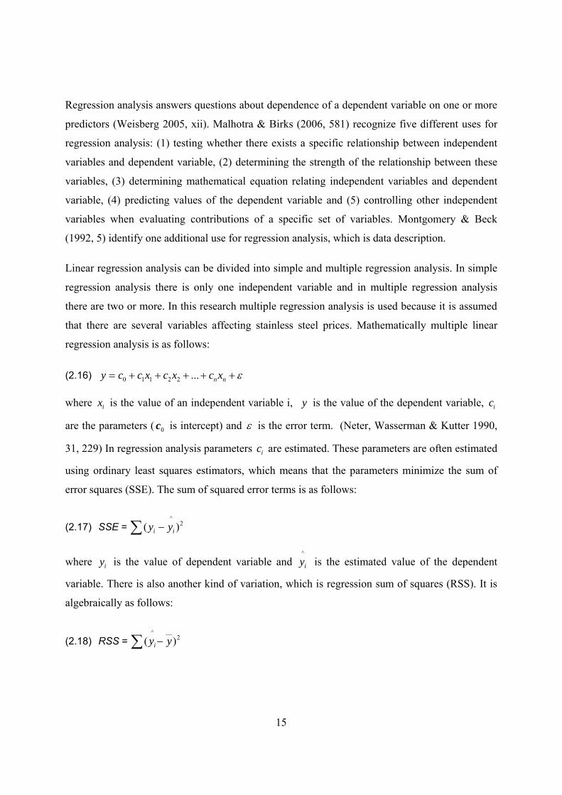
Linear regression analysis can be divided into simple and multiple regression analysis. In simple
regression analysis there is only one independent variable and in multiple regression analysis
there are two or more. In this research multiple regression analysis is used because it is assumed
that there are several variables affecting stainless steel prices. Mathematically multiple linear
regression analysis is as follows:
(2.16) ε+++++= nnxcxcxccy ...22110
where ix is the value of an independent variable i, y is the value of the dependent variable, ic
are the parameters ( 0c is intercept) and ε is the error term. (Neter, Wasserman & Kutter 1990,
31, 229) In regression analysis parameters ic are estimated. These parameters are often estimated
using ordinary least squares estimators, which means that the parameters minimize the sum of
error squares (SSE). The sum of squared error terms is as follows:
(2.17) SSE = ∑ − 2^
)( ii yy
where iy is the value of dependent variable and ^
iy is the estimated value of the dependent
variable. There is also another kind of variation, which is regression sum of squares (RSS). It is
algebraically as follows:
(2.18) RSS = ∑ − 2__^
)( yyi
16
where ^
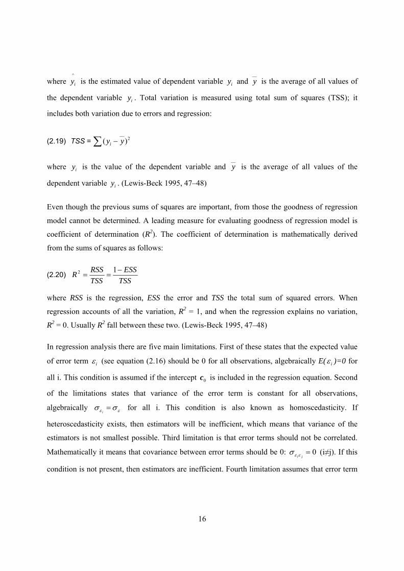
iy is the estimated value of dependent variable iy and __
y is the average of all values of
the dependent variable iy . Total variation is measured using total sum of squares (TSS); it
includes both variation due to errors and regression:
(2.19) TSS = ∑ − 2__
)( yyi
where iy is the value of the dependent variable and __
y is the average of all values of the
dependent variable iy . (Lewis-Beck 1995, 47–48)
Even though the previous sums of squares are important, from those the goodness of regression
model cannot be determined. A leading measure for evaluating goodness of regression model is
coefficient of determination (R2). The coefficient of determination is mathematically derived
from the sums of squares as follows:
(2.20) TSS
ESSTSSRSSR −
==12
where RSS is the regression, ESS the error and TSS the total sum of squared errors. When
regression accounts of all the variation, R2 = 1, and when the regression explains no variation,
R2 = 0. Usually R2 fall between these two. (Lewis-Beck 1995, 47–48)
In regression analysis there are five main limitations. First of these states that the expected value
of error term iε (see equation (2.16) should be 0 for all observations, algebraically E( iε )=0 for
all i. This condition is assumed if the intercept 0c is included in the regression equation. Second
of the limitations states that variance of the error term is constant for all observations,
algebraically εε σσ =i
for all i. This condition is also known as homoscedasticity. If
heteroscedasticity exists, then estimators will be inefficient, which means that variance of the
estimators is not smallest possible. Third limitation is that error terms should not be correlated.
Mathematically it means that covariance between error terms should be 0: 0=jiεεσ (i≠j). If this
condition is not present, then estimators are inefficient. Fourth limitation assumes that error term
17
is distributed independently of independent variables, algebraically 0=iix εσ . The last limitation
is that the error term should be normally distributed. (Dougherty 2002, 77–79)
There are several abuses of regression analysis that can be made. Three common misapplications
are extrapolation, generalization and causation. Extrapolation of data means predicting values of
dependent variable with values of independent variables that are not in the range of data.
Generalization occurs when researcher is trying to use results of regression analysis from a body
of data to make inferences for another body of data. The danger here is that the two bodies of
data might not possess the same characteristics. The reason for generalization being improper is
that there are extraneous factors affecting the dependent variable that regression analysis doesn’t
cover. Causation as an abuse of regression analysis exists when researcher concludes that a
dependent variable is explained by an independent variable, even though the correlation is due to
some other variables. (Gunst & Mason 1980; 12–18) This causation is a major problem in
scientific publications according to Ferson, Sarkissian & Simin (2003), as they argue that many
of the regressions in literature may be spurious. By spurious regression is meant that correlated
variables are used to explain some variable, even though there is no causation.
Berry & Feldman (1985, 18, 26, 37, 51) recognize also other abuses, or rather causes of abuses in
regression analysis. These are specification error, measurement error, multicollinearity, non-
additivity and non-linearity. Specification error occurs when a researcher assumes a specific
incorrect relationship between the independent variables and the dependent variable.
Measurement error can be divided into random and nonrandom parts. Random measurement error
is just unsystematic noise in the variables. Nonrandom measurement error occurs if researcher is
in some degree systematically measuring some variable wrong. (Berry & Feldman 1985, 18, 26)
Multicollinearity is a statistical phenomenon in which two or more independent variables in a
multiple regression model are highly correlated. Multicollinearity increases standard error of
estimates, and thus reduces degree of confidence. However, it does not result in biased estimates.
(Sykes 1999) Multicollinearity as a problem depends on the use of regression analysis. If
researcher uses regression analysis to predict values, multicollinearity is of a little problem.
However, if regression analysis is used for explanation, then multicollinearity might be of a
serious problem. (Berry & Feldman 1985, 40–41)
18
Regression analysis is based on additivity and linearity characteristics. The best way to detect
non-additivity and non-linearity is to compare the model to the theory underlying the model. If
linear model is not adequate, then there are two common options. In first, the linear model is
replaced by some other model, such as polynomial model or exponential model. (Berry &
Feldman 1985, 53, 57, 60) On the second option the independent variable used in the regression
model can be a function of the value of the original independent variable. For example, log X can
be used instead of X. (Farnum & Stanton 1989, 251)
2.3 Product Costing
In this subchapter different aspects of product costing are discussed, because they are important
in order to recognize what the best perspective in product costing is. For example, the choice
between full and variable costing can have major impact on business performance as will be
observed in the following. Whether full or variable costing is chosen, method of costing still
needs to be determined. Costing methods are based, for example, on market prices or marginal
costs. In this chapter actual methods of calculating product costs are discussed too. These
methods of calculating product costs include, for example, theory of constraints (TOC)
accounting and activity-based costing (ABC). Different methods calculate product costs
differently and are applicable in different situations, and thus these methods are needed to be
considered in order to find out the best method suited to the situation at hand.
2.3.1 Different Aspects of Product Costing
The objective of product costing is to set costs as near as possible to real costs of products.
However, for example, due to lack of data, this is seldom possible. Also real costs itself is a
theoretical concept. There are various errors associated with product costing. First, specification
error arises when the method used to identify costs to products does not reflect demands placed
on the resources by individual products. For example, if a product really needs one unit of
resource A, but in the product costing it has been allocated two units of the resource, there is a
specification error. (Datar & Gupta 1994) Manufacturing a product requires resources that do not
vary directly with the volume (e.g. setups). Aggregation errors occur when costs and units of a
resource are aggregated over heterogeneous activities to derive a single cost allocation rate.
(Foster & Gupta 1990) Specification and aggregation errors increase demand for more refined
19
costing systems. But there is a drawback in the modern accounting systems; the measurement
costs are increased. So there is a tradeoff between exactness of product costing and costs of
measurement. (Datar & Gupta 1994)
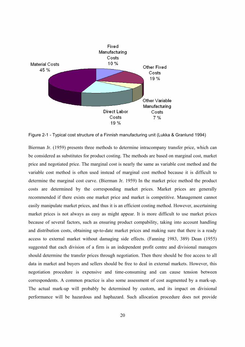
Product costs can be divided into many dimensions. First of all, there are fixed and variable costs.
Fixed costs are costs that are independent of amount of resources used and variable costs depend
linearly on the amount of resources used. The so-called traditional cost accounting literature often
suggests that product costing should be based on variable costing, because it offers more usable
and flexible information for decision-making than full costing (Lukka & Granlund 1996). Full
cost is the sum of allocated fixed costs and variable costs. Major weakness of the full costing is
that full costs lead user department to evaluate the full cost and benefit rather than marginal cost
and benefit. (Miller & Buckman 1987) Full costing also often considers historical sunk costs
rather than the future outlay of costs (McLaney & Atrill 1999, 312). Variable costing has the
desired property that operating departments are encouraged to expand their use until marginal
cost exceeds marginal benefit (Miller & Buckman 1987). As Fanning (1983, 167) confirms,
maximum profit will be earned where marginal revenue is equal to marginal cost. However, there
exists some critique towards variable costing. Zimmerman (1979) argues that variable costing
may form delays and rationing costs on other users within the company. So, allocating also fixed
costs according to actual usage may be desired since these allocated costs can serve as a useful
estimation for opportunity costs, which are difficult to observe due to delay and rationing
(Zimmerman 1979). Also full costing provides long-run relevant costs (McLaney & Atrill 1999,
312). In Finnish companies fixed costs are around 30 percent according to Lukka & Granlund
(1994) (Figure 2-1). Thus choosing full or variable costing has a real significance.
20
Figure 2-1 - Typical cost structure of a Finnish manufacturing unit (Lukka & Granlund 1994)
Bierman Jr. (1959) presents three methods to determine intracompany transfer price, which can
be considered as substitutes for product costing. The methods are based on marginal cost, market
price and negotiated price. The marginal cost is nearly the same as variable cost method and the
variable cost method is often used instead of marginal cost method because it is difficult to
determine the marginal cost curve. (Bierman Jr. 1959) In the market price method the product
costs are determined by the corresponding market prices. Market prices are generally
recommended if there exists one market price and market is competitive. Management cannot
easily manipulate market prices, and thus it is an efficient costing method. However, ascertaining
market prices is not always as easy as might appear. It is more difficult to use market prices
because of several factors, such as ensuring product compability, taking into account handling
and distribution costs, obtaining up-to-date market prices and making sure that there is a ready
access to external market without damaging side effects. (Fanning 1983, 389) Dean (1955)
suggested that each division of a firm is an independent profit centre and divisional managers
should determine the transfer prices through negotiation. Then there should be free access to all
data in market and buyers and sellers should be free to deal in external markets. However, this
negotiation procedure is expensive and time-consuming and can cause tension between
correspondents. A common practice is also some assessment of cost augmented by a mark-up.
The actual mark-up will probably be determined by custom, and its impact on divisional
performance will be hazardous and haphazard. Such allocation procedure does not provide
21
guidelines for efficient allocation of resources between divisions. (Fanning 1983, 388–389)
According to Fanning (1983, 387) transfer price method should depend at least on the following
factors: existence of an external market price for product, market structure in which company
operates and degree of interdependence between divisions.
2.3.2 Methods of Calculating Product Costs
The previously discussed different aspects of product costing do not provide exact information on
how to calculate the product costs in different methods. Now the methods of calculating product
costs are covered.
The ways of calculating product cost structure include theory of constraints accounting (TOC)
and activity based costing (ABC). They both represent alternative paradigms. Principle of TOC
assumes that every organization has a constraint or bottleneck that restricts its performance. In
TOC accounting performance of the company is improved by efficiently organizing this
bottleneck because TOC takes into account the use of constraints in forming product costs. (Kee
& Schmidt 2000) The benefits of TOC are as follows: (1) increasing revenue by increasing the
volume of production, (2) reducing cost per unit through increasing the production overall by
maximizing efficiency of the bottleneck, (3) management’s time is allocated to the area that
needs the most attention, which is often the bottleneck (Mekong Capital 2005). Firms that have
adopted TOC confirm that it has aided in reducing lead-time, cycle time and inventory, while
improving productivity and quality (Jayson 1987).
Activity based costing (ABC) system models causal relationship between products and resources
used in their production. ABC identifies activities that compose overhead costs and charges each
product for the quantity of each activity it consumed. The advantage of ABC is that it provides
more accurate information of product costs for evaluating the profitability of the company's
product lines and customer base. (Kee & Schmidt 2000) According to Cooper & Kaplan (1991,
130) management can thus analyze how products, brands, customers, facilities, regions and
distribution channels generate revenues and consume processes.
Traditional accounting system allocates overheads to product costs using volume-sensitive cost
drivers, such as direct labor (Kee & Schmidt 2000). Traditional costing is seen to be inconsistent
with today’s manufacturing methods (e.g. Monden & Lee 1993; Ferrara 1995). This is because
22
traditional costing is not able to provide appropriate strategic signals for business enterprises
(Fleischman and Tyson 1998). It may lead to dysfunctional behavior, for example, by
encouraging bulk purchasing, which leads to high inventories (Lucas 1997). However, standard
costing is still in common use even in very developed countries, such as Japan (Sulaiman, Ahmad
& Alwi 2006).
There is no single method recommended to be used in all situations; on the contrary, the choice
of method should depend on overall situation (Kee & Schmidt 2000). Some researchers argue
that TOC should be used for short-term planning and ABC for long-term planning (Lea &
Fredendall 2002). Lea’s (1998) study indicated that TOC did not perform adequately when there
were significant overheads, labor costs and automation involved in the manufacturing process.
Campbell, Brewer and Mills (1997) recommended TOC for machine-intensive departments
because costs of these departments are formed from creating and maintaining long-term capacity.
In machine-intensive departments allocation of fixed costs to products is not appropriate because
in managing constant resources time is a relevant measure, not money (Campbell, et al. 1997).
When product mix decision is considered, Kee & Schmidt (2000) argue that relative performance
of TOC and ABC accounting depend on the extent of management’s control over labor and
overhead.
Traditional costing system can underestimate costs of low volume products that have many levels
in bill-of-material and require many supporting activities. It can consequently allocate too large a
percentage of overhead costs to a high volume product with a flat bill-of-material. (Johnson,
1991; O’Guin, 1991) TOC ignores product structure and does not attempt to allocate support
function costs to products. So, TOC may avoid cost distortions related to allocating overheads,
but it may create another type of cost distortion if a product has low raw material costs and a high
sales price, but requires intensive support and technology investment. ABC might provide more
accurate product costs when products differ in their breadth and depth since ABC tracks all
activities used by all components of each product and charges the products only for activities that
were consumed. (Lea & Fredendall 2002) However, the main disadvantage of ABC costing is the
difficulty of obtaining accurate information to determine proper allocations (Hundal 1997). It has
also been argued that ABC requires detailed activity analysis, and thus if ABC is implemented
there is a significant need of changes in cost accounting systems (Sheldon, Huang & Perks 1991).
23
Theory of product costing has now been covered. As was mentioned previously, inventory
valuation is highly related to product costing. In the next section different inventory valuation
methods are analyzed.
2.4 Inventory Valuation Methods
Determining inventory valuation method that best fits to the circumstances faced is essential. Tax
shield benefits can be huge and precision of management accounting measures can be improved
much by just choosing appropriate inventory valuation method. So recognizing possible methods
to value inventory and analyzing those is needed if the current inventory valuation is to be
improved.
There are basically four GAAP cost flow assumptions: (1) specific identification; (2) first-in,
first-out (FIFO); (3) last-in, first-out (LIFO); and (4) weighted average cost (Wilson & Walter
2003). GAAP (Generally Accepted Accounting Principles) is the common set of accounting
principles, standards and procedures that companies use to compile their financial statements.
These four methods are now introduced and briefly analyzed one at a time. After that some other
possibilities for inventory valuation methods are presented. In the final part these methods are
compared with each other and optimal methods in different situations are analyzed.
2.4.1 Specific identification
Specific identification method requires matching each item sold with its actual costs. Items in
inventory are specifically set to cost the total costs of ending inventory (Simple Studies 2007). It
is a simple and workable method for businesses selling a few high priced items such as cars or
jewelry, but it is not practical when tracking high volume, low priced items such as units of crude
oil or natural gas (Wilson & Walter 2003). The challenge in raw material or other high volume
material accounting is to keep track of different purchase prices, which is not convenient in
specific identification (Simple Studies 2007). As an example, Amazon, having a high volume but
also some one-of-a-kind business, values inventory by using specific identification (Pollard,
Mills & Harrison 2007, 411).
The main advantage of specific identification is that it provides good matching between costs and
revenues. Some accountants argue that specific identification is the most precise accounting
24
method in matching the costs and revenues, and therefore it is theoretically the soundest method.
This statement is true for any one-of-a-kind items, and for these items any other accounting
method would seem illogical. (Hermanson et al. 2005, 273)
However, specific identification has its disadvantages. One of the main disadvantages, even
concerning one-of-a-kind items, is the possibility of manipulation. For example, if a company
would buy two identical items with different prices from supplier, there needs to be chosen which
one of the items is sold first to a customer. A manager optimizing his own utility will choose as
he prefers, and this can distort financial statements. For example, if a car dealer has two identical
cars with different costs, profit of the sale for those cars would be different, even though the cars
are identical. (Hermanson et al. 2005, 273; Simple Studies 2007)
2.4.2 First-In First-Out
In FIFO it is assumed that inventory in hand includes the items last purchased (Wilson & Walter
2003). For example, consider the following situation. A company has an opening inventory of
100 items and the inventory value is 100€, 1€ per an item. If in the current period company buys
100 items at the price of 2€, but sells 80 items, inventory by FIFO method is valued at (100-
80)*1€+100*2€=220€. The inventory for valuation purposes includes 20 items from the initial
inventory and all the 100 items bought in the current period.
FIFO has four major advantages: (1) it is easy to apply, (2) the flow of costs corresponds with the
physical flow of goods, (3) there is no possibility of manipulation and (4) amount of inventory in
balance sheet is likely to be approximately market value. All these advantages are due to the fact
that when a company sells goods, the costs removed from the inventory are the oldest units when
inventory valuation is considered. Company or manager cannot manipulate figures by pure
accounting tricks because the costs removed are not determined by a serial number. (Hermanson
et al. 2005, 273) The easiness in adaptation is also essential. In FIFO the reports are ready fast
and thus making decisions based on inventory is faster (Francis 2001). Only the FIFO method is
in line with the recommended way in which the materials should be physically issued. All other
methods are purely methods of pricing. (Chadwick 2002, 196)
The two main disadvantages of FIFO are (1) recognition of paper profits and (2) heavier tax
burden under inflation (Hermanson et al. 2005, 273). By paper profits it is meant the difference
25
between the costs of a replacement unit and the historical cost of the unit. For example, say a
company has three identical items in inventory in order of purchase time purchase prices being
1€, 2€ and 4€. FIFO would allocate a cost of 1€ to the next sale and LIFO a cost of 4€. LIFO is
covered in next chapter. The difference of 4€-1€=3€ represents paper profits in FIFO compared
to LIFO. The heavier tax burden under inflation results from the fact that the inventory in hand
includes the last purchases, which are the most valuable. Thus in net income calculation costs
allocated to sales are the least valuable, which increases profits and thus tax obligations. (Wilson
& Walter 2003)
2.4.3 Last-In First-Out
In LIFO inventory in hand includes the first purchases (Wilson & Walter 2003). Let’s consider
the same example as in the beginning of section 2.4.2. In LIFO inventory value is 100*1€+(100-
80)*2€=140€, which is quite different from value by FIFO method (220€).
LIFO has several advantages, which are based on the fact that prices have risen almost constantly
for decades. LIFO supporters argue that this upward trend in prices leads to paper profits under
FIFO, thus making LIFO more appealing. (Hermanson et al. 2005, 273) Opposite to FIFO, LIFO
also brings tax benefits under inflation (Pollard et al. 2007, 413). Another advantage of LIFO is
that the costs allocated to products are the most recent and reflect reality. By LIFO, company
performance can better be evaluated, because the cost of goods sold and thus net income is based
on the current situation. (Hermanson et al. 2005, 274) Due to the reflection of reality, writing
down of inventory to market price is minimized (Robertson & Clark 2004).
Disadvantages of LIFO according to FIFO supporters include the following: (1) LIFO doesn’t
reflect physical flow of goods, (2) LIFO understates inventory and (3) LIFO permits income
manipulation. There is a continuous debate on whether physical and cost flow should reflect each
other. The second criticism is valid under rising prices, especially if inventory in LIFO includes
items several periods ago. Income manipulation criticism is also valid. For example, if it is
assumed that management wishes to reduce income, the company purchases an abnormal amount
of items at the end of the previous period, whereby the costs of goods in the next period are high.
Vice versa, management could delay purchases to increase income. (Hermanson et al. 2005, 274)
Robertson & Clark (2004) mention also that LIFO may cause poor buying habits because of layer
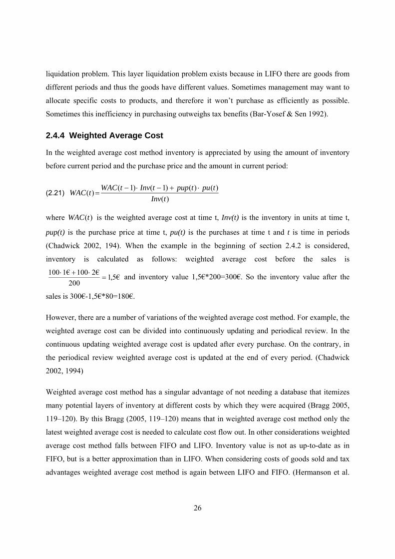
26
liquidation problem. This layer liquidation problem exists because in LIFO there are goods from
different periods and thus the goods have different values. Sometimes management may want to
allocate specific costs to products, and therefore it won’t purchase as efficiently as possible.
Sometimes this inefficiency in purchasing outweighs tax benefits (Bar-Yosef & Sen 1992).
2.4.4 Weighted Average Cost
In the weighted average cost method inventory is appreciated by using the amount of inventory
before current period and the purchase price and the amount in current period:
(2.21) )(
)()()1()1()(
tInvtputpuptInvtWAC
tWAC⋅+−⋅−
=
where )(tWAC is the weighted average cost at time t, Inv(t) is the inventory in units at time t,
pup(t) is the purchase price at time t, pu(t) is the purchases at time t and t is time in periods
(Chadwick 2002, 194). When the example in the beginning of section 2.4.2 is considered,
inventory is calculated as follows: weighted average cost before the sales is
€5,1200
€2100€1100=
⋅+⋅ and inventory value 1,5€*200=300€. So the inventory value after the
sales is 300€-1,5€*80=180€.
However, there are a number of variations of the weighted average cost method. For example, the
weighted average cost can be divided into continuously updating and periodical review. In the
continuous updating weighted average cost is updated after every purchase. On the contrary, in
the periodical review weighted average cost is updated at the end of every period. (Chadwick
2002, 1994)
Weighted average cost method has a singular advantage of not needing a database that itemizes
many potential layers of inventory at different costs by which they were acquired (Bragg 2005,
119–120). By this Bragg (2005, 119–120) means that in weighted average cost method only the
latest weighted average cost is needed to calculate cost flow out. In other considerations weighted
average cost method falls between FIFO and LIFO. Inventory value is not as up-to-date as in
FIFO, but is a better approximation than in LIFO. When considering costs of goods sold and tax
advantages weighted average cost method is again between LIFO and FIFO. (Hermanson et al.
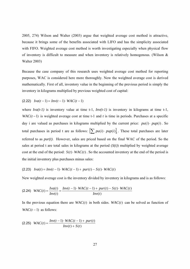
27
2005, 274) Wilson and Walter (2003) argue that weighted average cost method is attractive,
because it brings some of the benefits associated with LIFO and has the simplicity associated
with FIFO. Weighted average cost method is worth investigating especially when physical flow
of inventory is difficult to measure and when inventory is relatively homogenous. (Wilson &
Walter 2003)
Because the case company of this research uses weighted average cost method for reporting
purposes, WAC is considered here more thoroughly. Now the weighted average cost is derived
mathematically. First of all, inventory value in the beginning of the previous period is simply the
inventory in kilograms multiplied by previous weighted cost of capital:
(2.22) )1()1()1( −⋅−=− tWACtInvtIva
where Iva(t-1) is inventory value at time t-1, Inv(t-1) is inventory in kilograms at time t-1,
)1( −tWAC is weighted average cost at time t-1 and t is time in periods. Purchases at a specific
day i are valued as purchases in kilograms multiplied by the current price: )()( ipupipu ⋅ . So
total purchases in period t are as follows: [ ]t
ipupipu∑ ⋅ )()( . These total purchases are later
referred to as pur(t). However, sales are priced based on the final WAC of the period. So the
sales at period t are total sales in kilograms at the period (S(t)) multiplied by weighted average
cost at the end of the period: )()( tWACtS ⋅ . So the accounted inventory at the end of the period is
the initial inventory plus purchases minus sales:
(2.23) )()()()1()1()( tWACtStpurtWACtInvtIva ⋅−+−⋅−=
New weighted average cost is the inventory divided by inventory in kilograms and is as follows:
(2.24) )(
)()()()1()1()()()(
tInvtWACtStpurtWACtInv
tInvtIvatWAC ⋅−+−⋅−==
In the previous equation there are )(tWAC in both sides. )(tWAC can be solved as function of
)1( −tWAC as follows:
(2.25) )()(
)()1()1()(tStInv
tpurtWACtInvtWAC+
+−⋅−=
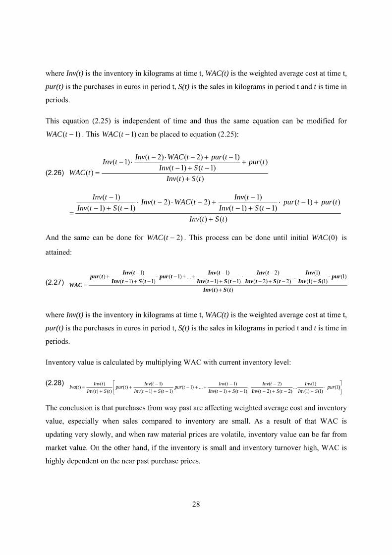
28
where Inv(t) is the inventory in kilograms at time t, WAC(t) is the weighted average cost at time t,
pur(t) is the purchases in euros in period t, S(t) is the sales in kilograms in period t and t is time in
periods.
This equation (2.25) is independent of time and thus the same equation can be modified for
)1( −tWAC . This )1( −tWAC can be placed to equation (2.25):
(2.26) )()(
)()1()1(
)1()2()2()1()(
tStInv
tpurtStInv
tpurtWACtInvtInvtWAC
+
+−+−
−+−⋅−⋅−
=
)()(
)()1()1()1(
)1()2()2()1()1(
)1(
tStInv
tpurtpurtStInv
tInvtWACtInvtStInv
tInv
+
+−⋅−+−
−+−⋅−⋅
−+−−
=
And the same can be done for )2( −tWAC . This process can be done until initial )0(WAC is
attained:
(2.27) )()(
)1()1()1(
)1(...)2()2(
)2()1()1(
)1(...)1()1()1(
)1()(
tStInv
purSInv
InvtStInv
tInvtStInv
tInvtpurtStInv
tInvtpurWAC
+
⋅+−+−
−⋅
−+−−
++−⋅−+−
−+
=
where Inv(t) is the inventory in kilograms at time t, WAC(t) is the weighted average cost at time t,
pur(t) is the purchases in euros in period t, S(t) is the sales in kilograms in period t and t is time in
periods.
Inventory value is calculated by multiplying WAC with current inventory level:
(2.28) ⎥⎦
⎤⎢⎣
⎡⋅
+−+−−
⋅−+−
−++−
−+−−
++
= )1()1()1(
)1(...)2()2(
)2()1()1(
)1(...)1()1()1(
)1()()()(
)()( purSInv
InvtStInv
tInvtStInv
tInvtpurtStInv
tInvtpurtStInv
tInvtIva
The conclusion is that purchases from way past are affecting weighted average cost and inventory
value, especially when sales compared to inventory are small. As a result of that WAC is
updating very slowly, and when raw material prices are volatile, inventory value can be far from
market value. On the other hand, if the inventory is small and inventory turnover high, WAC is
highly dependent on the near past purchase prices.
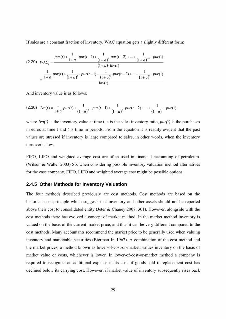
29
If sales are a constant fraction of inventory, WAC equation gets a slightly different form:
(2.29) ( ) ( )( ) )(1
)1(1
1...)2(1
1)1(1
1)( 12
tInva
pura
tpura
tpura
tpurWAC
t
t ⋅+
⋅+
++−+
+−⋅+
+=
−
( ) ( ) ( ))(
)1(1
1...)2(1
1)1(1
1)(1
132
tInv
pura
tpura
tpura
tpura t ⋅+
++−+
+−⋅+
++
=
And inventory value is as follows:
(2.30) ( ) ( ) ( )
)1(1
1...)2(1
1)1(1
1)(1
1)(32
pura
tpura
tpura
tpura
tIvat⋅
+++−
++−⋅
++
+=
where Iva(t) is the inventory value at time t, a is the sales-inventory-ratio, pur(t) is the purchases
in euros at time t and t is time in periods. From the equation it is readily evident that the past
values are stressed if inventory is large compared to sales, in other words, when the inventory
turnover is low.
FIFO, LIFO and weighted average cost are often used in financial accounting of petroleum.
(Wilson & Walter 2003) So, when considering possible inventory valuation method alternatives
for the case company, FIFO, LIFO and weighted average cost might be possible options.
2.4.5 Other Methods for Inventory Valuation
The four methods described previously are cost methods. Cost methods are based on the
historical cost principle which suggests that inventory and other assets should not be reported
above their cost to consolidated entity (Jeter & Chaney 2007, 301). However, alongside with the
cost methods there has evolved a concept of market method. In the market method inventory is
valued on the basis of the current market price, and thus it can be very different compared to the
cost methods. Many accountants recommend the market price to be generally used when valuing
inventory and marketable securities (Bierman Jr. 1967). A combination of the cost method and
the market prices, a method known as lower-of-cost-or-market, values inventory on the basis of
market value or costs, whichever is lower. In lower-of-cost-or-market method a company is
required to recognize an additional expense in its cost of goods sold if replacement cost has
declined below its carrying cost. However, if market value of inventory subsequently rises back
30
to or above carrying cost, recorded value cannot be increased back to the original amount. (Bragg
2005, 123) The advantage of the lower-of-cost-or-market method is that company is able to defer
some taxes for later periods if prices of goods decrease.
Neilimo & Uusi-Rauva (2005) mention two additional methods for inventory cost accounting.
These are price of the day and standard price. In the price of the day method cost flow out of
inventory is determined by the latest purchase price. This method is thus quite near the market
price method, but it uses previous purchase as a determinant, which can be several days or
months old. In standard price method cost flow is determined by a single standard price, which
should reflect the market price. The price is determined from long-term development of prices.
Especially in different scenario modeling standard price provides good guess for cost flow.
(Neilimo & Uusi-Rauva 2005, 93) Fry, Steele & Saladin (1996) propose that standard cost
system is applicable when direct costs, specifically labor, represent a large percentage of total
manufacturing costs. Standard cost is not appropriate when overhead costs from a major share of
total costs or when labor costs are relatively small (Fry, Steele & Saladin 1996).
By the previous analysis of inventory valuation methods it is not possible to choose the best
method in different situations and that is why in the next subsection inventory valuation methods
are compared based on previous analysis and literature.
2.4.6 Comparison of Inventory Valuation Methods
After getting familiar with the inventory valuation methods, it is important to compare these
methods with each other. First, the advantages and disadvantages of FIFO, LIFO and weighted
average cost method brought up in the previous subsections are analyzed. After that the factors
that should be taken into account when choosing an inventory valuation method are summarized.
One consideration in choosing the inventory valuation methods is implementation. Previously it
was mentioned that FIFO is easy to apply. This is partly because in FIFO there are not so much
layers in use as is in LIFO. The layers mean items having different prices, and thus they need to
be considered separately. LIFO may have several layers in use at the same time when the material
in inventory is far away from past, and thus that has to be considered in inventory calculations. In
the weighted average cost method inventory calculations are the simplest, because new weighted
average cost and inventory value depend only on the previous inventory and the latest sales and
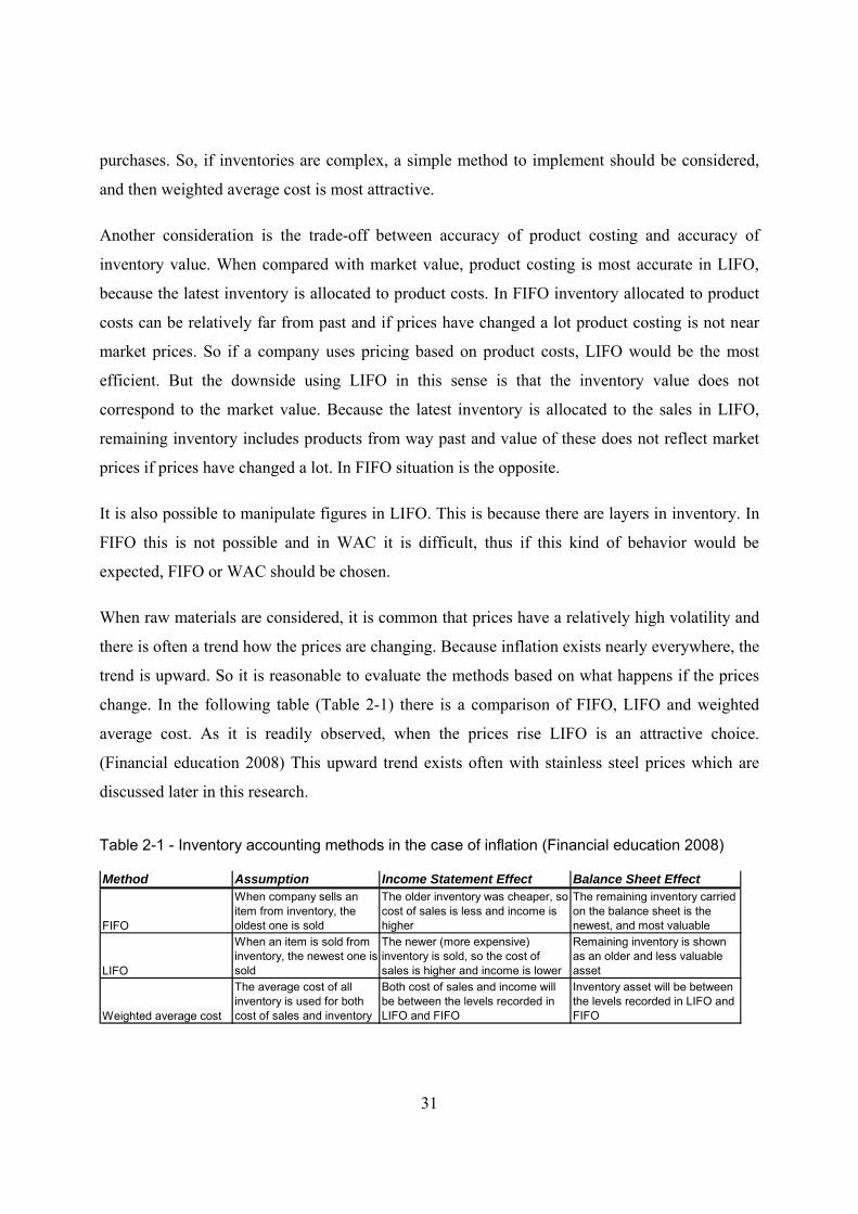
31
purchases. So, if inventories are complex, a simple method to implement should be considered,
and then weighted average cost is most attractive.
Another consideration is the trade-off between accuracy of product costing and accuracy of
inventory value. When compared with market value, product costing is most accurate in LIFO,
because the latest inventory is allocated to product costs. In FIFO inventory allocated to product
costs can be relatively far from past and if prices have changed a lot product costing is not near
market prices. So if a company uses pricing based on product costs, LIFO would be the most
efficient. But the downside using LIFO in this sense is that the inventory value does not
correspond to the market value. Because the latest inventory is allocated to the sales in LIFO,
remaining inventory includes products from way past and value of these does not reflect market
prices if prices have changed a lot. In FIFO situation is the opposite.
It is also possible to manipulate figures in LIFO. This is because there are layers in inventory. In
FIFO this is not possible and in WAC it is difficult, thus if this kind of behavior would be
expected, FIFO or WAC should be chosen.
When raw materials are considered, it is common that prices have a relatively high volatility and
there is often a trend how the prices are changing. Because inflation exists nearly everywhere, the
trend is upward. So it is reasonable to evaluate the methods based on what happens if the prices
change. In the following table (Table 2-1) there is a comparison of FIFO, LIFO and weighted
average cost. As it is readily observed, when the prices rise LIFO is an attractive choice.
(Financial education 2008) This upward trend exists often with stainless steel prices which are
discussed later in this research.
Table 2-1 - Inventory accounting methods in the case of inflation (Financial education 2008)
Method Assumption Income Statement Effect Balance Sheet Effect
FIFO
When company sells an item from inventory, the oldest one is sold
The older inventory was cheaper, so cost of sales is less and income is higher
The remaining inventory carried on the balance sheet is the newest, and most valuable
LIFO
When an item is sold from inventory, the newest one is sold
The newer (more expensive) inventory is sold, so the cost of sales is higher and income is lower
Remaining inventory is shown as an older and less valuable asset
Weighted average cost
The average cost of all inventory is used for both cost of sales and inventory
Both cost of sales and income will be between the levels recorded in LIFO and FIFO
Inventory asset will be between the levels recorded in LIFO and FIFO
32
In the 1970s hundreds of firms changed inventory valuation method to LIFO in response to high
rates of inflation. However, many still continued with FIFO method. (Lee & Hsieh 1985) Biddle
(1980) estimated that 105 firms investigated in his study paid an average of nearly $26 millions
in additional federal income tax. So there is something else than the potential tax benefits that
make firms to decide their inventory accounting policy. According to Lee & Hsieh (1985), the
choice of inventory accounting method is affected in addition to tax shield benefits by three
factors: political costs, agency costs and divergent production and investment characteristics.
According to Bar-Yosef & Sen (1992) an optimal accounting policy takes into account this
distortion (the incentive effect) as well as tax gains possible with LIFO. Whatever the choice of
inventory valuation method, switching is not easy and not easily reversed, especially in the case
of LIFO (Lee & Petruzzi 1989).
Potential determinants on decision of corporate inventory accounting according to Hunt (1985)
include the following two: (1) restrictive debt covenants and (2) the extent of managers being
owners. The restrictive debt covenants include restriction of dividend payments, asset
maintenance restrictions such as minimum working capital and restriction of financing policy
(e.g. increasing debt-equity-ratio) (Hunt 1985). Inventory affects these restrictions clearly. If
inventory value is low, working capital is lower and minimum working capital limit might be in
danger. When the limit of working capital is near and inflation exists, LIFO method can be
harmful because it values the inventory on the basis of the oldest items, which are valued the
lowest under inflation. Thus FIFO or weighted average cost method should be preferred. The
extent to which managers are owners affects the choice of the method. If the ownership is high,
management can choose the best method for their purposes. Therefore, if management
compensation is dependent on the income, the managers prefer income-increasing methods. (Kuo
1993) Niehaus (1989) argues that if managerial ownership is low, management can exercise little
discretion in choosing the method. LIFO is often selected if managerial ownership is low,
because it increases cash flow and value of the firm, and thus it is the method favored by outside
shareholders (Niehaus 1989). Astami & Tower (2006) confirmed in their research that the level
of ownership is an important factor in determining the inventory accounting policy.
Kuo (1993) listed several other potential determinants, of which the most important were
following: (1) potential tax savings, (2) capital structure, (3) firm size, (4) volatility of earnings,
33
(5) management’s compensation and (6) managers’ ownership. The greater the tax savings are
the greater the probability is that the company will find it easy to absorb or justify
implementation costs of a new inventory valuation method (Kuo 1993). These implementation
costs can be depreciated in a schedule depending on tax law. Thus if the tax savings are great, a
company might easily consider changes in inventory valuation methods.
These possible tax savings have an indirect effect on stock prices of companies in public
exchange. The better cash flow structure due to the benefits in tax obligations increases present
values of future cash flows. Thus there is often a temptation by managers to change the policy
into the direction that maximizes the stock price, and thus also their compensation if it is tied to
the stock price (Hughes, Fellingham & Schwartz 1988). Related to stock prices and the benefits
of tax shield, Krishnan, Srinidhi & Su (2008) investigated the effect of FIFO/LIFO choice on the
cost of capital of companies. In the research it was shown that LIFO firms have lower cost of
capital. This is because costs of goods sold are better matched to the current situation in LIFO.
More importantly, in FIFO the costs of goods sold include goods way past and from a longer
period, which brings more variation to the costs of goods sold, and thus increases volatility of
earnings. Also managers face lower variability which means that it is more risky for managers to
deliberately insert opportunistic discretionary accruals in LIFO to cost of goods sold account.
(Krishnan et al. 2008)
When the capital structure is considered, it is generally agreed that the larger the amount of debt
in a company's capital structure is, the greater the probability is that the company chooses an
income-increasing method (Dhaliwal 1980). The rationale behind this hypothesis is that adoption
of income-increasing accounting procedures would lower the probability of the firm getting into a
technical default (Kuo 1993). By the technical default Kuo (1993) means that a company might
go into bankruptcy because of accounting methods, not because of the real operations or
financing. Income-increasing method might be preferable also in another sense. Namely
companies have obligations to debt collectors, and when the debt is negotiated, the debtor is
easier convinced that the company does not default on the payments if the income for accounting
purposes is larger. All in all, when the company has a lot of debt, the method to be preferred
based on previous discussion is FIFO. (Kuo 1993)
34
Firm size also affects the choice of inventory valuation method. Dopuch & Pincus (1988) argue
that LIFO method involves high bookkeeping and tax reporting costs. Granof & Short (1984)
reported that more than 30 percent of companies in their non-LIFO sample rejected LIFO
because of “excessive costs” or “other adverse consequences”. A survey by Hilke (1986)
confirmed that these adoption costs of LIFO can be significant, in his survey adoption costs
ranged from 0,7 percent to 7,9 percent of average profits. These bookkeeping and tax reporting
costs are mostly fixed. Because of these fixed costs, larger companies have a comparative
advantage in adopting LIFO. So it is reasonable to assume that large companies more frequently
implement LIFO compared to small ones. (Kuo 1993) However, in a study by Astami & Tower
(2006), which included a relatively large sample of Asian companies, size of a company was not
a significant factor when inventory valuation policy was considered.
An increase in volatility of earnings increases the chance of a company reporting higher profits,
which in turn increases company's political exposure (Kuo 1993). This political exposure results
from the fact that companies reporting higher profits are more likely to be subjected to regulation
(Watts & Zimmermann 1978). To reduce political exposure, an income-decreasing method is
selected (Kuo 1993). Biddle (1980) argues that the most popular determinant for inventory
accounting method is smoothing of income stream. Variability of earnings affects the choice of
inventory valuation method in another way through business risk. It is reasonable that companies
facing business risks use income-decreasing methods, so that if the company faces hard times in
the future there is something left from the good times. (Kuo 1993)
A determinant of inventory valuation method not yet discussed is behavior of inventory in
particular aspects. Cushing & LeClere (1992) found that immateriality of inventory, inventory
variability and inventory obsolescence have an effect on the choice of the inventory valuation
method. Immateriality of inventory is higher with FIFO companies, but the significance of this
hypothesis is low. Inventory variability of FIFO companies is larger than with LIFO companies,
and FIFO companies have also more obsolescence in their inventory. (Cushing & LeClere 1992)
The bigger inventory variability in FIFO companies might be due to the fact that in FIFO
inventory is the latest, and because of having the latest purchases it varies more. Still, it seems
that the higher the risk with the inventory is, the more frequently FIFO is used.
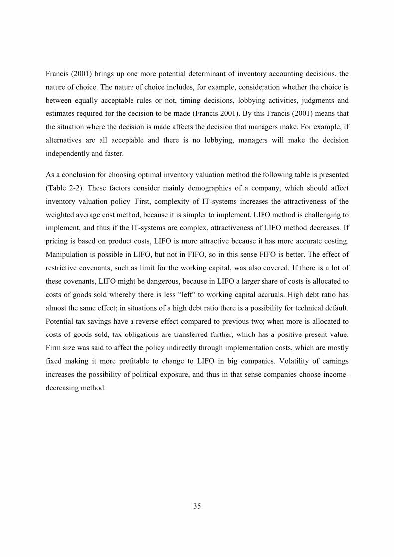
35
Francis (2001) brings up one more potential determinant of inventory accounting decisions, the
nature of choice. The nature of choice includes, for example, consideration whether the choice is
between equally acceptable rules or not, timing decisions, lobbying activities, judgments and
estimates required for the decision to be made (Francis 2001). By this Francis (2001) means that
the situation where the decision is made affects the decision that managers make. For example, if
alternatives are all acceptable and there is no lobbying, managers will make the decision
independently and faster.
As a conclusion for choosing optimal inventory valuation method the following table is presented
(Table 2-2). These factors consider mainly demographics of a company, which should affect
inventory valuation policy. First, complexity of IT-systems increases the attractiveness of the
weighted average cost method, because it is simpler to implement. LIFO method is challenging to
implement, and thus if the IT-systems are complex, attractiveness of LIFO method decreases. If
pricing is based on product costs, LIFO is more attractive because it has more accurate costing.
Manipulation is possible in LIFO, but not in FIFO, so in this sense FIFO is better. The effect of
restrictive covenants, such as limit for the working capital, was also covered. If there is a lot of
these covenants, LIFO might be dangerous, because in LIFO a larger share of costs is allocated to
costs of goods sold whereby there is less “left” to working capital accruals. High debt ratio has
almost the same effect; in situations of a high debt ratio there is a possibility for technical default.
Potential tax savings have a reverse effect compared to previous two; when more is allocated to
costs of goods sold, tax obligations are transferred further, which has a positive present value.
Firm size was said to affect the policy indirectly through implementation costs, which are mostly
fixed making it more profitable to change to LIFO in big companies. Volatility of earnings
increases the possibility of political exposure, and thus in that sense companies choose income-
decreasing method.
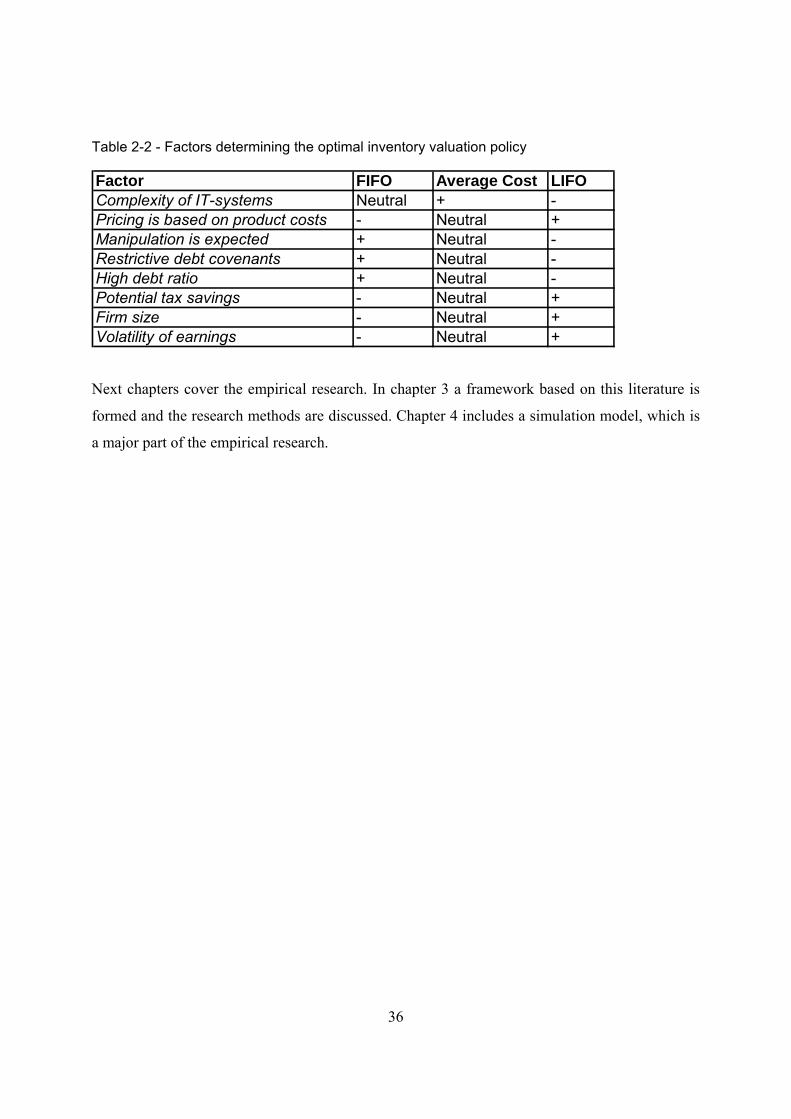
36
Table 2-2 - Factors determining the optimal inventory valuation policy
Factor FIFO Average Cost LIFOComplexity of IT-systems Neutral + -Pricing is based on product costs - Neutral +Manipulation is expected + Neutral -Restrictive debt covenants + Neutral -High debt ratio + Neutral -Potential tax savings - Neutral +Firm size - Neutral +Volatility of earnings - Neutral +
Next chapters cover the empirical research. In chapter 3 a framework based on this literature is
formed and the research methods are discussed. Chapter 4 includes a simulation model, which is
a major part of the empirical research.
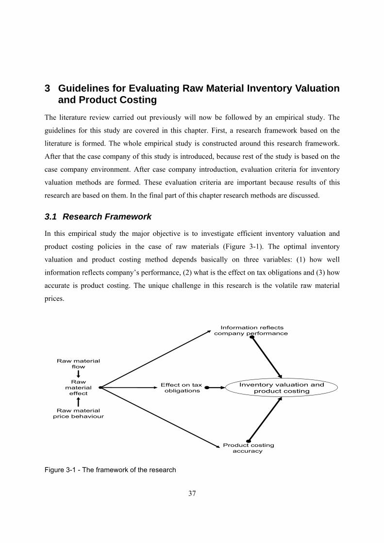
37
3 Guidelines for Evaluating Raw Material Inventory Valuation and Product Costing
The literature review carried out previously will now be followed by an empirical study. The
guidelines for this study are covered in this chapter. First, a research framework based on the
literature is formed. The whole empirical study is constructed around this research framework.
After that the case company of this study is introduced, because rest of the study is based on the
case company environment. After case company introduction, evaluation criteria for inventory
valuation methods are formed. These evaluation criteria are important because results of this
research are based on them. In the final part of this chapter research methods are discussed.
3.1 Research Framework
In this empirical study the major objective is to investigate efficient inventory valuation and
product costing policies in the case of raw materials (Figure 3-1). The optimal inventory
valuation and product costing method depends basically on three variables: (1) how well
information reflects company’s performance, (2) what is the effect on tax obligations and (3) how
accurate is product costing. The unique challenge in this research is the volatile raw material
prices.
Inventory valuation andproduct costing
Raw materialprice behaviour
Product costingaccuracy
Raw materialflow
Information reflectscompany performance
Raw material
effect
Effect on tax obligations
Figure 3-1 - The framework of the research
38
The main objective of management accounting is to give information for decision-makers. The
first variable (information reflects company performance) takes this into consideration. If the
inventory valuation and product costing policy give accurate information about the current
situation and the recent success of the company, this information can be trusted and thus
management can make reliable decisions based on the information. This information reliability
affects all business levels. At product level, if the costs are allocated to the products incorrectly, it
is impossible to compare profitabilities of these products. Because of these incorrectly calculated
product costs, management might withdraw some profitable and leave some unprofitable
products to the product line. Of course this decreases the profitability of the company.
When considering information accurateness on a business unit level, inaccurate inventory
valuation gives wrong impression of business unit performance. Then some business units seem
to be more profitable and some business units appear to be less profitable than they would be if
the information is correct. As a result management might try to improve business units that are
already very profitable, and leave some unprofitable business units uncontrolled which are really
in need of serious controlling. The situation can be even worse; management might harvest
profitable business units because of incorrect information.
In a company level the inaccuracy of inventory valuation will cause technical loss or profit in
short-term. By technical loss or profit it is meant that by a certain method balance sheet and
income statement differ when compared to another method. For example, if by a certain method
inventory value is 100 000 € larger than by some other method, then the company makes a
technical profit of 100 000 € by choosing the first method. This technical profit, or alternatively
loss, creates problems discussed in chapter 2.4.6. One example was that management
compensation is affected by this technical loss or profit, even though the performance of the
company stays the same. As was mentioned earlier, the management compensation should be
based on performance of the company.
Second variable in the framework is the effect on tax obligations. This variable is important
because a company can achieve major alterations in cash flows by changing inventory valuation
policy. These alterations are due to the fact that different methods value inventory in different
ways. When by a certain method inventory value changes only a little, for example, increases by
1000 € and by a another method increase is 10 000 €, then by the latter method the increase in
39
inventory is 9000 € more. This larger increase produces profit and of course more taxes have to
be paid then.
Especially if the raw material prices are volatile, there can be huge differences in tax obligations
between different inventory valuation methods. Also inflation affects considerably these
differences. But what is the most important thing is that these different tax obligations have
different present values. So when considering the effect of the tax obligations, present value of all
tax obligations must be calculated. The method that has the smallest present value of tax
obligations is the best.
Third, pricing is often based on product costs. Thus product costs need to be as accurate as
possible. If the costs are not accurate, pricing is neither optimal. Because of inaccurate product
costing company might sell goods that are priced too high or low, and thus lose customers or
make loss. Products can include a lot of raw material, and when the price of the raw material
changes, product costs should also change. If these product costs are seldom updated, they can be
far from real values. Even if the company updates raw material prices continuously, the prices are
still not usually optimal. This is due to the fact that the raw material costs are allocated to the
product when it is transferred from raw material inventory. Yet, the product is sold to a customer
after it is produced and a customer has been found. Therefore there is a time lag between the
moments when the cost of raw material is allocated to the product and when the product is sold.
So, it is important that allocated costs reflect the market situation when the end-product is sold.
3.2 Case Company Introduction
This subchapter first introduces the case company of this research, which is Metos Finland Oy.
After that the Metos’ current inventory valuation and product costing are covered.
3.2.1 Metos Finland Oy
Metos is a developer and marketer of solutions and equipment designed for professional kitchens
for efficient and high quality food and beverage production. Metos is the market leader in the
industry in Nordic Countries. Metos has its own sales companies in Finland, Sweden, Norway,
France, Netherlands, Belgium, the Great Britain, Russia, Estonia, Lithuania and Latvia. In
addition Metos has a large group of representatives in other countries. The company’s factories
40
are situated in Finland, Sweden, Estonia, Netherlands and Belgium. Metos has about 900
employees and its turnover is 160 million euros. Metos is owned by its parent company Ali
Group, which is the market leader in professional kitchen industry in Europe. It has a turnover of
765 million euros and personnel of about 3900. (Metos intranet 2008)
In addition to the strong service concept Metos has a vast production. The main equipments sold
include combi-kettles and dishwashing equipment and systems. Other areas of emphasis in
Metos’ production are ranges and bratt pans as well as equipment for food retailing, transport and
catering for institutional and restaurant use. To produce such end-products a large amount of
stainless steel is needed. Price of stainless steel has been very volatile for the past years, and thus
product costing and inventory valuation have been recently losing reliability. (Metos intranet
2008) Because Metos is surely not the only one who is struggling with this kind of problems, the
subject is really worth investigating.
3.2.2 Inventory Valuation and Product Costing at Metos Finland Oy
Metos’ raw material inventory is valued by using two different methods. First, the parent
company of Metos uses weighted average cost in inventory valuation, and thus Metos needs to
report stainless steel inventory by using that method. Due to this, the weighted average cost
method is used in ERP-systems at Metos. However, when the inventory is valued for other
purposes, another method referred to here as 3-month average method, is used. In the 3-month
average method inventory unit value is the average of the stainless steel prices of the three
previous months. All prices are weighted equally. Inventory value is obtained by multiplying this
inventory unit value by inventory units (kilograms).
What comes to product costing, there are review sessions when total product costs of a certain
end-product are set for the next period. Often this period is one year. Total product costs are
constant during the period. However, stainless steel as a part of the costs is not constant. The
stainless steel cost is determined by the inventory valuation method of the 3-month average
explained above. The stainless steel cost is unit cost based on 3-month average multiplied by the
amount that the end-product uses stainless steel.
41
3.3 Evaluation Criteria of Inventory Valuation Methods
In this chapter evaluation criteria for the inventory valuation methods are developed. They are
based on the research framework presented in the previous chapter. Following four criteria are
included in the evaluation criteria: (1) inventory value fluctuation due to stainless steel price, (2)
product costing accurateness, (3) inventory value difference with weighted average cost method
and (4) present value of tax obligations.
The inventory value fluctuation here means the change in inventory values between successive
periods. This change is due to two components: (1) change in raw material amount and (2)
change in raw material prices. Raw material amounts change a lot and it is due to purchasing
habits. The change due to raw material price fluctuation has nothing to do with performance of
the company. So, changes in value at raw material inventory due to change in raw material price
distort performance measures, and therefore it has to be minimized. So, one criterion is the
inventory value fluctuation due to stainless steel price, which describes how much inventory
fluctuates due to stainless steel price movements.
The foremost objective of product costing is to match up product costs as near to real costs as
possible. This is essential if pricing is based on product costs. Costs of stainless steel are
allocated to an end-product when the stainless steel goes out of raw material inventory. However,
the end-product is priced and sold later. The time between the flow out of the raw material
inventory and selling the end-product is commonly determined from days of supply between raw
material inventory and customer. There are three main spots where the days of supply is created,
and they are end-product inventory, logistics (mainly transporting) and production. Summing
these days of supplies together, an average time between allocating product costs and selling end-
product is obtained. From the data of the case company it can be observed that the days of
supplies are on the average 1,3 months for end-product inventory and 1,2 months for logistics.
Adding also work-in-progress in production, the sum of the days of supplies is around three
months. So, the transfer price from raw material inventory three months before sales has to be
comparable to market price at the time of sales. The criterion used here is to compare transfer
price and market price three months after and it is called product costing accurateness.
42
The third evaluation criterion is based on the situation in the case company. The case company
uses weighted average cost method in reporting, because the parent company and subsidiaries use
that method too. The chosen inventory valuation method has to produce values near to the values
obtained by weighted average cost method, otherwise there will be major differences between the
reported inventory value and the inventory value used for other purposes. This difference cannot
be allocated to any time period or any products and that’s why it is very unwanted difference in
the case company. Therefore, the difference between weighted average cost and the chosen
method is the third evaluation criterion and it is called inventory value difference with weighted
average cost method.
The final criterion is based on the fact that inventory valuation method affects tax shield as
mentioned in the chapter 2.4. Tax shield gives opportunity to transfer tax obligations to later
periods. If taxes can be transferred to later periods, the present value of these obligations is lower.
The net present value of this benefit is considered as a final criterion and it is called present value
of tax obligations.
3.4 Research Method of Empirical Study
The evaluation criteria imply that the research problem is quantitative, and thus quantitative
research methods are used in this research to solve the research problem. In order to efficiently
carry out this research, features of quantitative research methods are covered in the next section.
The objective of this research is to give instructions to choose the method that is most beneficial
in future. In order to evaluate future with a lot of uncertainties, simulation was chosen as the
quantitative research method. Therefore simulation as a research method is introduced in section
3.4.2.
3.4.1 Quantitative Research Methods
Quantitative research is used to investigate questions related to quantities and percentages and
relations between different research objects or changes in research matters. This implies that a
sample needs to be big enough to represent adequately the subject being investigated. (Heikkilä
2001, 16) Therefore, in the simulation model a large number of simulations are needed.
According to Nau (1995) quantitative research look for distinguishing characteristics, elemental
properties and empirical boundaries and tend to measure how much or how often pertaining the
43
research object. Thus quantitative research can be construed as a research strategy that
emphasizes quantification in collection and analysis of data (Bryman & Bell 2003, 25).
Quantitative research methods include, for example, a mail questionnaire and a www-
questionnaire. These are surveys. Quantitative research can also be observational, where the
information is gathered by making observations about the object of the research. (Heikkilä 2001,
18–19)
Quantitative research has many advantages. First, not like qualitative research methods, in
quantitative research there is independence between researcher and subject being observed. Also,
comparison and replication are possible in quantitative methods, and partly due to this, reliability
and validity may be determined more objectively than in qualitative techniques. These
comparison and replication are a special strength in this study because a number of future
scenarios can be tested and compared by simulation. In quantitative methodologies the subject
under analysis is measured by objective methods rather than being inferred through sensation,
reflection or intuition. Also when compared to some qualitative methods, like expensive
interviews, in quantitative methods the cost and effort can be a lot less. (Amaratunga, Baldry,
Sarshar & Newton 2002)
Weaknesses of quantitative research include lack of ascertaining deeper underlying meanings and
explanations (Amaratunga et al. 2002). This can lead to incorrect conclusions if the subject of the
research is not familiar to the researcher. Often by using quantitative research methods
reasonings associated with the situation are not discovered. (Heikkilä 2001, 16) However, in this
research these weaknesses are not important. Literature review before this empirical study gave a
deeper understanding of the subject, and by this deeper understanding reasonings behind the
situation can be analyzed with the help of the simulation model.
3.4.2 Simulation as a Research Method
In this chapter the quantitative research method of this research, simulation, is covered.
Simulation is imitation of an operation in a real-world process or system over time (Banks,
Carson, Nelson & Nicol 2005, 3). The most significant feature of simulation is that it allows
imitating one process by a more easily arranged process (Hartmann 2005).
44
Computer simulation is growing in popularity as a research method. There are many reasons for
this popularity. First of all, many real-world problems are so complex that there is no possibility
of solving these problems analytically. One advantage of simulation is that in simulation there is
often no need to make assumptions about exact cause and effect of the system under study as it is
in other research methods. (Dooley 2002) However, Banks et al. (2005, 3) confirm that a
simulation model usually needs a set of assumptions concerning operation of the system, but less
than in other methods. This makes it possible to study more complex issues. Especially in this
empirical study the problem is not possible to solve analytically, because there are many complex
causalities and uncertainties. If a lot of assumptions are formed, solutions of this research would
not be reliable.
Whereas other studies try to explain how something happened, simulation answers to the
question what if something happens. This leads to another advantage in simulation research:
“moving future” makes it possible to test various kinds of scenarios for future. (Dooley 2002)
Because the focus in this study is in the future, the “moving future” is essential. In simulation, for
example, new hardware designs, layouts, policies and operation procedures can be tested without
committing resources or disrupting ongoing process. In simulation time can be compressed,
interactions of variables can be attained and bottleneck analysis can be done to increase
knowledge. But the major use of simulation is that it can help to understand how the system
operates. (Shannon 1992)
However, even though there are many advantages in using simulation, few disadvantages also
exist. First of all, model building requires special skills. Simulation results are also difficult to
interpret. Especially differentiating results of system interaction and randomness might be
challenging. Simulation modeling and analysis can be time-consuming and increase costs
heavily. Simulation is also often used even though it is not reasonable and there are analytical
solutions. (Banks et al. 2005, 6) Because of these disadvantages, there was a versatile preparation
done for the simulations. First, researcher familiarized himself all-around with simulation as a
research method and the problem at hand. By this preparation the skills to build the simulation
model were acquired. In order to obtain more accurate results, the number of replications was
high. To interpret the results easily, an unambiguous evaluation criteria based on literature was
developed (see section 3.3).
45
Before using simulation as a tool, it needs to be analyzed whether simulation as a method is
appropriate. Banks & Gibson (1997) formed the following ten rules for determining when
simulation is not appropriate. Simulation should not be used when the problem can be solved by
common sense or analytically, or on the other hand, when the problem is too complex to be
simulated. Simulation is not reasonable when real-world experiment is more easily or less costly
done, or if costs exceed savings due to simulation. Another method than simulation should be
used if there are not enough resources or data available for simulation, or not enough time to use
the results from simulation. Simulation is not appropriate if simulation model can’t be verified or
validated, or simulation project expectations cannot be met. (Banks & Gibson 1997) In
preparation for the simulation it was observed that none of these features exists in the simulation
model.
Although there are many factors eliminating the use of simulation, there are still many situations
when simulation is useful. Many authors have discussed this, and the following list of eleven
possible purposes of simulation is a summary by Banks et al. (2005, 4). Especially items 1, 4, 6
and 11 were exploited in this research.
1. Simulation enables experimentation with internal interactions of a complex system.
2. Informational, organizational and environmental changes can be simulated, and the effect
of these can be observed.
3. Knowledge that evolves when designing simulation model can be used for improving
system under investigation.
4. Changing simulation inputs and observing outputs can produce valuable insight for
determining interactions of variables.
5. Simulation can be used as a pedagogical device to reinforce analytical solution
methodologies.
6. Simulation can be used to test new designs or policies before implementation.
7. Simulation can be used to verify analytical solutions.
8. Simulating different capabilities of a machine can help to determine requirements for it.
9. Simulation models designed to educational purposes can ease learning process with less
cost and disruption.
10. Simulation can be used to visualize behavior of a system.

46
11. Modern systems can be so complex that its internal interactions are sometimes
discovered only through simulation. (Banks et al. 2005, 4)
Based on the previous discussion simulation was chosen as the research method for the empirical
part of this study. In the next chapter the simulation model is introduced and in chapter 5 results
of the simulation are presented.
47
4 Simulation Model to Evaluate Inventory Valuation Methods This chapter introduces the simulation model developed for evaluating different inventory
valuation methods. By this simulation model inventory valuation and product costing can be
tested under volatile raw material prices. The purpose of this empirical research is to investigate
possible stainless steel inventory valuation methods.
Simulation model of this research can characterized as an input-output-model. In this chapter the
inputs and the model are covered. The outputs of the model are presented in chapter 5. In section
4.1 data used for modeling the inputs is introduced. In section 4.2 the main input is modeled,
which is the stainless steel price. In modeling stainless steel prices it was observed that the prices
depend largely on nickel prices, and therefore in section 4.3 nickel prices are modeled. Thereafter
rest of the inputs, purchase and production behavior, are modeled in section 4.4. The simulation
model itself is introduced in section 4.5.
4.1 Data Used in Simulation Model
In building the simulation model various data was used. The quantitative data used included
material flow of stainless steel, stainless steel prices and data acquired from public sources. The
material flow data was acquired from the case company. Purchases were obtained from a
financial management software called eOffice. This purchase data was in euros, but it was easily
converted to kilograms with the help of stainless steel price data. Production data was gathered
from the production department. It was already in kilograms. Stainless steel prices depend on
customer and the prices that Metos pays were obtained from the purchasing department.
The data acquired from public sources included data for the regression model in chapter 4.2. This
data includes nickel price, chrome price, global nickel inventory and $/€-ratio data. Nickel price
data was obtained from Metalsmarket (2008). Chrome and global nickel inventory data was
obtained from Metalprices (2008) and $/€-ratio data was acquired from Oanda (2008). This
public source data is available all-around world.
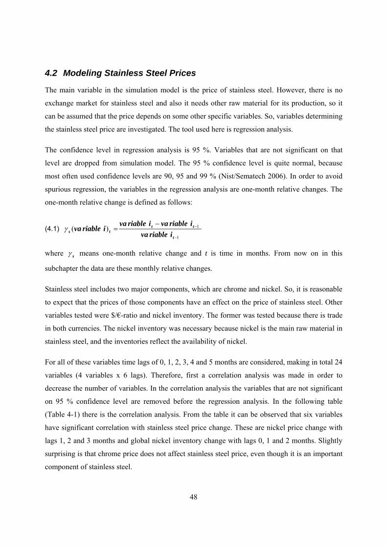
48
4.2 Modeling Stainless Steel Prices
The main variable in the simulation model is the price of stainless steel. However, there is no
exchange market for stainless steel and also it needs other raw material for its production, so it
can be assumed that the price depends on some other specific variables. So, variables determining
the stainless steel price are investigated. The tool used here is regression analysis.
The confidence level in regression analysis is 95 %. Variables that are not significant on that
level are dropped from simulation model. The 95 % confidence level is quite normal, because
most often used confidence levels are 90, 95 and 99 % (Nist/Sematech 2006). In order to avoid
spurious regression, the variables in the regression analysis are one-month relative changes. The
one-month relative change is defined as follows:
(4.1) 1
1)(−
−−=
t
ttts iriableva
iriablevairiablevairiablevaγ
where sγ means one-month relative change and t is time in months. From now on in this
subchapter the data are these monthly relative changes.
Stainless steel includes two major components, which are chrome and nickel. So, it is reasonable
to expect that the prices of those components have an effect on the price of stainless steel. Other
variables tested were $/€-ratio and nickel inventory. The former was tested because there is trade
in both currencies. The nickel inventory was necessary because nickel is the main raw material in
stainless steel, and the inventories reflect the availability of nickel.
For all of these variables time lags of 0, 1, 2, 3, 4 and 5 months are considered, making in total 24
variables (4 variables x 6 lags). Therefore, first a correlation analysis was made in order to
decrease the number of variables. In the correlation analysis the variables that are not significant
on 95 % confidence level are removed before the regression analysis. In the following table
(Table 4-1) there is the correlation analysis. From the table it can be observed that six variables
have significant correlation with stainless steel price change. These are nickel price change with
lags 1, 2 and 3 months and global nickel inventory change with lags 0, 1 and 2 months. Slightly
surprising is that chrome price does not affect stainless steel price, even though it is an important
component of stainless steel.
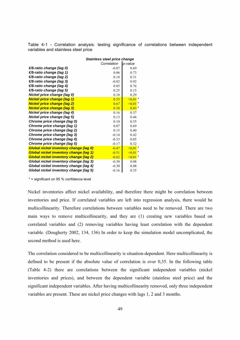
49
Table 4-1 - Correlation analysis: testing significance of correlations between independent variables and stainless steel price
Stainless steel price changeCorrelation p-value
€/$-ratio change (lag 0) -0.07 0.69€/$-ratio change (lag 1) 0.06 0.73€/$-ratio change (lag 2) 0.18 0.31€/$-ratio change (lag 3) -0.02 0.92€/$-ratio change (lag 4) 0.05 0.76€/$-ratio change (lag 5) 0.25 0.15Nickel price change (lag 0) 0.18 0.29Nickel price change (lag 1) 0.53 <0,01 *Nickel price change (lag 2) 0.67 <0,01 *Nickel price change (lag 3) 0.38 0.03 *Nickel price change (lag 4) 0.16 0.37Nickel price change (lag 5) 0.13 0.46Chrome price change (lag 0) 0.10 0.55Chrome price change (lag 1) 0.07 0.69Chrome price change (lag 2) 0.15 0.40Chrome price change (lag 3) -0.14 0.42Chrome price change (lag 4) -0.33 0.05Chrome price change (lag 5) -0.17 0.32Global nickel inventory change (lag 0) -0.47 <0,01 *Global nickel inventory change (lag 1) -0.51 <0,01 *Global nickel inventory change (lag 2) -0.62 <0,01 *Global nickel inventory change (lag 3) -0.30 0.08Global nickel inventory change (lag 4) -0.30 0.08Global nickel inventory change (lag 5) -0.16 0.35
* = significant on 95 % confidence level
Nickel inventories affect nickel availability, and therefore there might be correlation between
inventories and price. If correlated variables are left into regression analysis, there would be
multicollinearity. Therefore correlations between variables need to be removed. There are two
main ways to remove multicollinearity, and they are (1) creating new variables based on
correlated variables and (2) removing variables having least correlation with the dependent
variable. (Dougherty 2002, 134, 136) In order to keep the simulation model uncomplicated, the
second method is used here.
The correlation considered to be multicollinearity is situation-dependent. Here multicollinearity is
defined to be present if the absolute value of correlation is over 0,35. In the following table
(Table 4-2) there are correlations between the significant independent variables (nickel
inventories and prices), and between the dependent variable (stainless steel price) and the
significant independent variables. After having multicollinearity removed, only three independent
variables are present. These are nickel price changes with lags 1, 2 and 3 months.
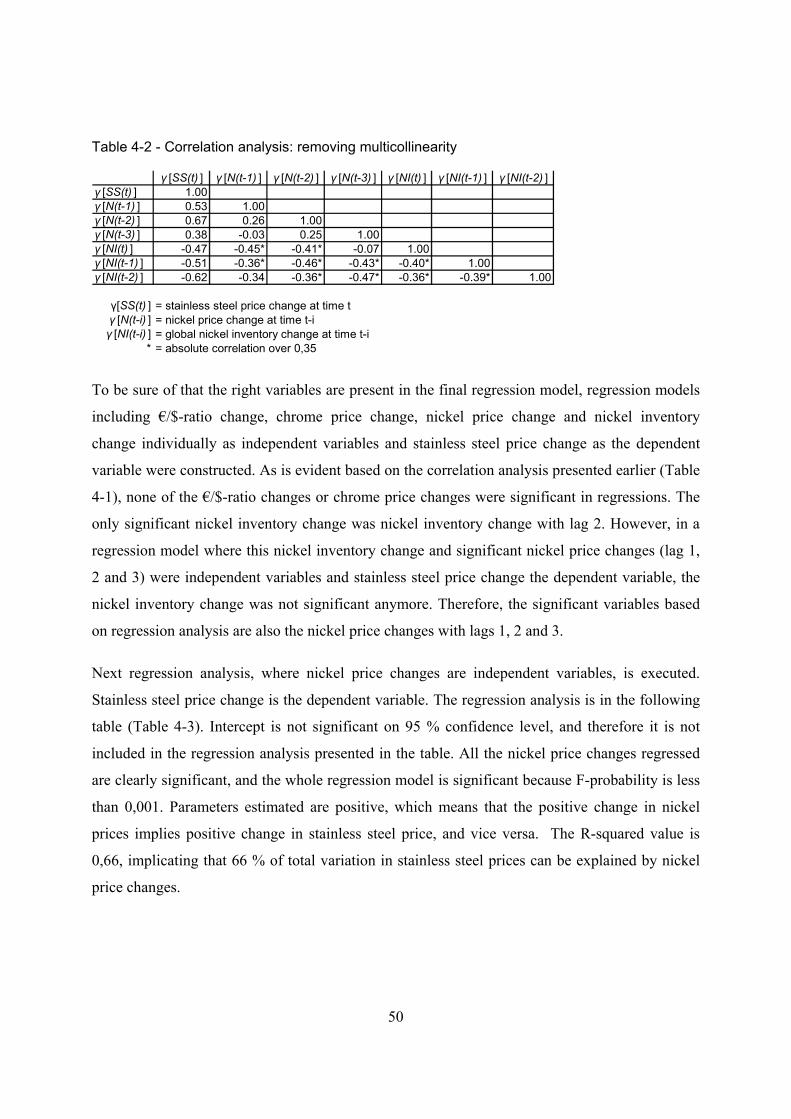
50
Table 4-2 - Correlation analysis: removing multicollinearity
γ [SS(t) ] γ [N(t-1) ] γ [N(t-2) ] γ [N(t-3) ] γ [NI(t) ] γ [NI(t-1) ] γ [NI(t-2) ]γ [SS(t) ] 1.00γ [N(t-1) ] 0.53 1.00γ [N(t-2) ] 0.67 0.26 1.00γ [N(t-3) ] 0.38 -0.03 0.25 1.00γ [NI(t) ] -0.47 -0.45* -0.41* -0.07 1.00γ [NI(t-1) ] -0.51 -0.36* -0.46* -0.43* -0.40* 1.00γ [NI(t-2) ] -0.62 -0.34 -0.36* -0.47* -0.36* -0.39* 1.00
γ[SS(t) ] = stainless steel price change at time tγ [N(t-i) ] = nickel price change at time t-iγ [NI(t-i) ] = global nickel inventory change at time t-i
* = absolute correlation over 0,35
To be sure of that the right variables are present in the final regression model, regression models
including €/$-ratio change, chrome price change, nickel price change and nickel inventory
change individually as independent variables and stainless steel price change as the dependent
variable were constructed. As is evident based on the correlation analysis presented earlier (Table
4-1), none of the €/$-ratio changes or chrome price changes were significant in regressions. The
only significant nickel inventory change was nickel inventory change with lag 2. However, in a
regression model where this nickel inventory change and significant nickel price changes (lag 1,
2 and 3) were independent variables and stainless steel price change the dependent variable, the
nickel inventory change was not significant anymore. Therefore, the significant variables based
on regression analysis are also the nickel price changes with lags 1, 2 and 3.
Next regression analysis, where nickel price changes are independent variables, is executed.
Stainless steel price change is the dependent variable. The regression analysis is in the following
table (Table 4-3). Intercept is not significant on 95 % confidence level, and therefore it is not
included in the regression analysis presented in the table. All the nickel price changes regressed
are clearly significant, and the whole regression model is significant because F-probability is less
than 0,001. Parameters estimated are positive, which means that the positive change in nickel
prices implies positive change in stainless steel price, and vice versa. The R-squared value is
0,66, implicating that 66 % of total variation in stainless steel prices can be explained by nickel
price changes.
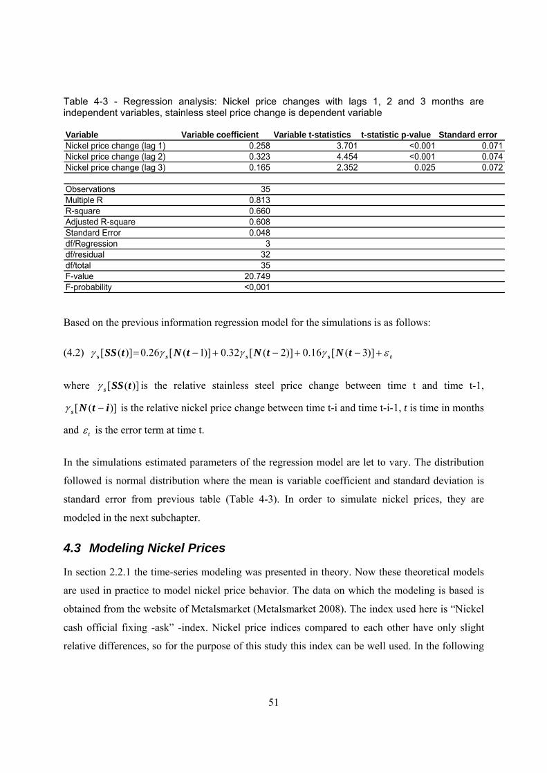
51
Table 4-3 - Regression analysis: Nickel price changes with lags 1, 2 and 3 months are independent variables, stainless steel price change is dependent variable
Variable Variable coefficient Variable t-statistics t-statistic p-value Standard errorNickel price change (lag 1) 0.258 3.701 <0.001 0.071Nickel price change (lag 2) 0.323 4.454 <0.001 0.074Nickel price change (lag 3) 0.165 2.352 0.025 0.072
Observations 35Multiple R 0.813R-square 0.660Adjusted R-square 0.608Standard Error 0.048df/Regression 3df/residual 32df/total 35F-value 20.749F-probability <0,001
Based on the previous information regression model for the simulations is as follows:
(4.2) tssss tNtNtNtSS εγγγγ +−+−+−= )]3([16.0)]2([32.0)]1([26.0)]([
where )]([ tSSsγ is the relative stainless steel price change between time t and time t-1,
)]([ itNs −γ is the relative nickel price change between time t-i and time t-i-1, t is time in months
and tε is the error term at time t.
In the simulations estimated parameters of the regression model are let to vary. The distribution
followed is normal distribution where the mean is variable coefficient and standard deviation is
standard error from previous table (Table 4-3). In order to simulate nickel prices, they are
modeled in the next subchapter.
4.3 Modeling Nickel Prices
In section 2.2.1 the time-series modeling was presented in theory. Now these theoretical models
are used in practice to model nickel price behavior. The data on which the modeling is based is
obtained from the website of Metalsmarket (Metalsmarket 2008). The index used here is “Nickel
cash official fixing -ask” -index. Nickel price indices compared to each other have only slight
relative differences, so for the purpose of this study this index can be well used. In the following
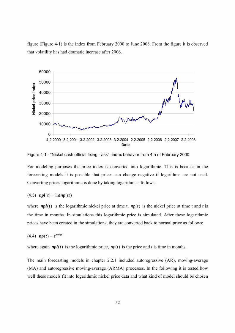
52
figure (Figure 4-1) is the index from February 2000 to June 2008. From the figure it is observed
that volatility has had dramatic increase after 2006.
0
10000
20000
30000
40000
50000
60000
4.2.2000 3.2.2001 3.2.2002 3.2.2003 3.2.2004 2.2.2005 2.2.2006 2.2.2007 2.2.2008Date
Nick
el p
rice
inde
x
Figure 4-1 - “Nickel cash official fixing - ask” -index behavior from 4th of February 2000
For modeling purposes the price index is converted into logarithmic. This is because in the
forecasting models it is possible that prices can change negative if logarithms are not used.
Converting prices logarithmic is done by taking logarithm as follows:
(4.3) ))(ln()( tnptnpl =
where )(tnpl is the logarithmic nickel price at time t, )(tnp is the nickel price at time t and t is
the time in months. In simulations this logarithmic price is simulated. After these logarithmic
prices have been created in the simulations, they are converted back to normal price as follows:
(4.4) )()( tnpletnp =
where again )(tnpl is the logarithmic price, )(tnp is the price and t is time in months.
The main forecasting models in chapter 2.2.1 included autoregressive (AR), moving-average
(MA) and autoregressive moving-average (ARMA) processes. In the following it is tested how
well these models fit into logarithmic nickel price data and what kind of model should be chosen
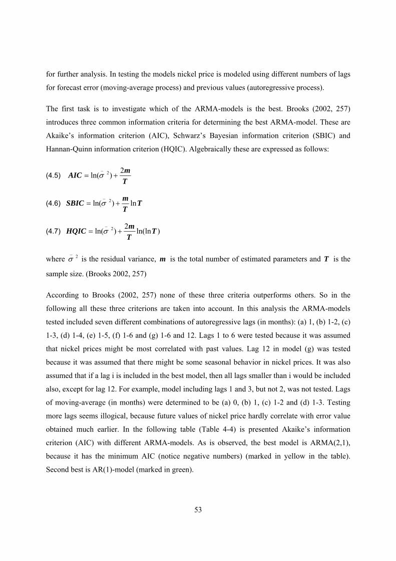
53
for further analysis. In testing the models nickel price is modeled using different numbers of lags
for forecast error (moving-average process) and previous values (autoregressive process).
The first task is to investigate which of the ARMA-models is the best. Brooks (2002, 257)
introduces three common information criteria for determining the best ARMA-model. These are
Akaike’s information criterion (AIC), Schwarz’s Bayesian information criterion (SBIC) and
Hannan-Quinn information criterion (HQIC). Algebraically these are expressed as follows:
(4.5) TmAIC 2)ln( 2
_+= σ
(4.6) TTmSBIC ln)ln( 2
_+= σ
(4.7) )ln(ln2)ln( 2_
TTmHQIC += σ
where 2_σ is the residual variance, m is the total number of estimated parameters and T is the
sample size. (Brooks 2002, 257)
According to Brooks (2002, 257) none of these three criteria outperforms others. So in the
following all these three criterions are taken into account. In this analysis the ARMA-models
tested included seven different combinations of autoregressive lags (in months): (a) 1, (b) 1-2, (c)
1-3, (d) 1-4, (e) 1-5, (f) 1-6 and (g) 1-6 and 12. Lags 1 to 6 were tested because it was assumed
that nickel prices might be most correlated with past values. Lag 12 in model (g) was tested
because it was assumed that there might be some seasonal behavior in nickel prices. It was also
assumed that if a lag i is included in the best model, then all lags smaller than i would be included
also, except for lag 12. For example, model including lags 1 and 3, but not 2, was not tested. Lags
of moving-average (in months) were determined to be (a) 0, (b) 1, (c) 1-2 and (d) 1-3. Testing
more lags seems illogical, because future values of nickel price hardly correlate with error value
obtained much earlier. In the following table (Table 4-4) is presented Akaike’s information
criterion (AIC) with different ARMA-models. As is observed, the best model is ARMA(2,1),
because it has the minimum AIC (notice negative numbers) (marked in yellow in the table).
Second best is AR(1)-model (marked in green).
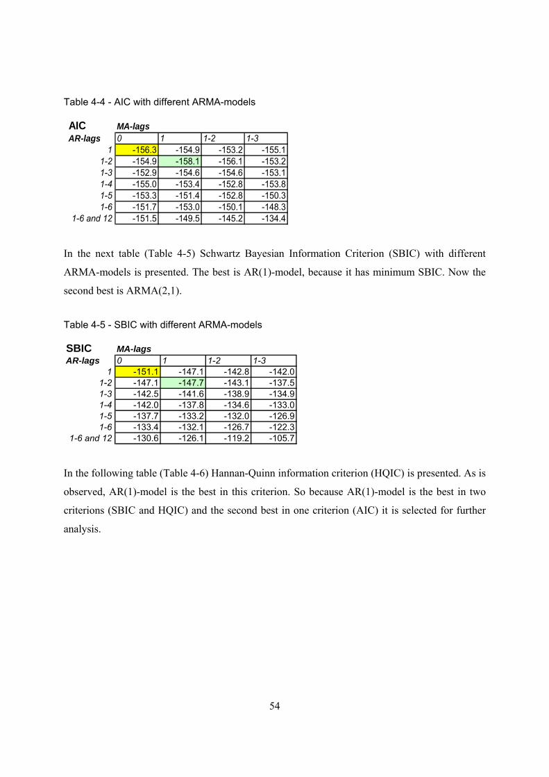
54
Table 4-4 - AIC with different ARMA-models
AIC MA-lagsAR-lags 0 1 1-2 1-3
1 -156.3 -154.9 -153.2 -155.11-2 -154.9 -158.1 -156.1 -153.21-3 -152.9 -154.6 -154.6 -153.11-4 -155.0 -153.4 -152.8 -153.81-5 -153.3 -151.4 -152.8 -150.31-6 -151.7 -153.0 -150.1 -148.3
1-6 and 12 -151.5 -149.5 -145.2 -134.4
In the next table (Table 4-5) Schwartz Bayesian Information Criterion (SBIC) with different
ARMA-models is presented. The best is AR(1)-model, because it has minimum SBIC. Now the
second best is ARMA(2,1).
Table 4-5 - SBIC with different ARMA-models
SBIC MA-lagsAR-lags 0 1 1-2 1-3
1 -151.1 -147.1 -142.8 -142.01-2 -147.1 -147.7 -143.1 -137.51-3 -142.5 -141.6 -138.9 -134.91-4 -142.0 -137.8 -134.6 -133.01-5 -137.7 -133.2 -132.0 -126.91-6 -133.4 -132.1 -126.7 -122.3
1-6 and 12 -130.6 -126.1 -119.2 -105.7
In the following table (Table 4-6) Hannan-Quinn information criterion (HQIC) is presented. As is
observed, AR(1)-model is the best in this criterion. So because AR(1)-model is the best in two
criterions (SBIC and HQIC) and the second best in one criterion (AIC) it is selected for further
analysis.
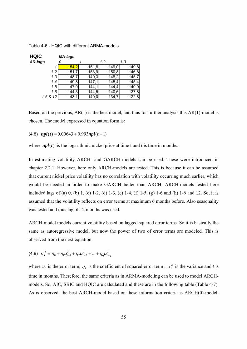
55
Table 4-6 - HQIC with different ARMA-models
HQIC MA-lagsAR-lags 0 1 1-2 1-3
1 -154,2 -151,8 -149,0 -149,81-2 -151,7 -153,9 -150,8 -146,81-3 -148,7 -149,3 -148,2 -145,71-4 -149,8 -147,1 -145,4 -145,41-5 -147,0 -144,1 -144,4 -140,91-6 -144,3 -144,5 -140,6 -137,8
1-6 & 12 -143,1 -140,0 -134,7 -122,8
Based on the previous, AR(1) is the best model, and thus for further analysis this AR(1)-model is
chosen. The model expressed in equation form is:
(4.8) )1(993.000643.0)( −+= tnpltnpl
where )(tnpl is the logarithmic nickel price at time t and t is time in months.
In estimating volatility ARCH- and GARCH-models can be used. These were introduced in
chapter 2.2.1. However, here only ARCH-models are tested. This is because it can be assumed
that current nickel price volatility has no correlation with volatility occurring much earlier, which
would be needed in order to make GARCH better than ARCH. ARCH-models tested here
included lags of (a) 0, (b) 1, (c) 1-2, (d) 1-3, (e) 1-4, (f) 1-5, (g) 1-6 and (h) 1-6 and 12. So, it is
assumed that the volatility reflects on error terms at maximum 6 months before. Also seasonality
was tested and thus lag of 12 months was used.
ARCH-model models current volatility based on lagged squared error terms. So it is basically the
same as autoregressive model, but now the power of two of error terms are modeled. This is
observed from the next equation:
(4.9) 2222
2110
2 ... qtqttt uuu −−− ++++= ηηηησ
where tu is the error term, iη is the coefficient of squared error term , 2tσ is the variance and t is
time in months. Therefore, the same criteria as in ARMA-modeling can be used to model ARCH-
models. So, AIC, SBIC and HQIC are calculated and these are in the following table (Table 4-7).
As is observed, the best ARCH-model based on these information criteria is ARCH(0)-model,
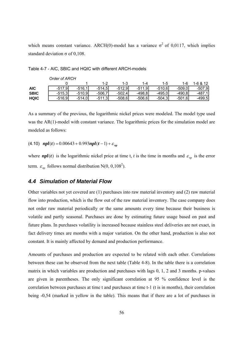
56
which means constant variance. ARCH(0)-model has a variance σ2 of 0,0117, which implies
standard deviation σ of 0,108.
Table 4-7 - AIC, SBIC and HQIC with different ARCH-models
Order of ARCH0 1 1-2 1-3 1-4 1-5 1-6 1-6 & 12
AIC -517,9 -516,1 -514,5 -512,9 -511,9 -510,6 -509,0 -507,9SBIC -515,3 -510,9 -506,7 -502,4 -498,8 -495,0 -490,8 -487,1HQIC -516,9 -514,0 -511,3 -508,6 -506,6 -504,3 -501,6 -499,5
As a summary of the previous, the logarithmic nickel prices were modeled. The model type used
was the AR(1)-model with constant variance. The logarithmic prices for the simulation model are
modeled as follows:
(4.10) nptnpltnpl ε+−+= )1(993.000643.0)(
where )(tnpl is the logarithmic nickel price at time t, t is the time in months and npε is the error
term. npε follows normal distribution N(0, 0,1082).
4.4 Simulation of Material Flow
Other variables not yet covered are (1) purchases into raw material inventory and (2) raw material
flow into production, which is the flow out of the raw material inventory. The case company does
not order raw material periodically or the same amounts every time because their business is
volatile and partly seasonal. Purchases are done by estimating future usage based on past and
future plans. In purchases volatility is increased because stainless steel deliveries are not exact, in
fact delivery times are months with a major variation. On the other hand, production is also not
constant. It is mainly affected by demand and production performance.
Amounts of purchases and production are expected to be related with each other. Correlations
between these can be observed from the next table (Table 4-8). In the table there is a correlation
matrix in which variables are production and purchases with lags 0, 1, 2 and 3 months. p-values
are given in parentheses. The only significant correlation at 95 % confidence level is the
correlation between purchases at time t and purchases at time t-1 (t is in months), their correlation
being -0,54 (marked in yellow in the table). This means that if there are a lot of purchases in
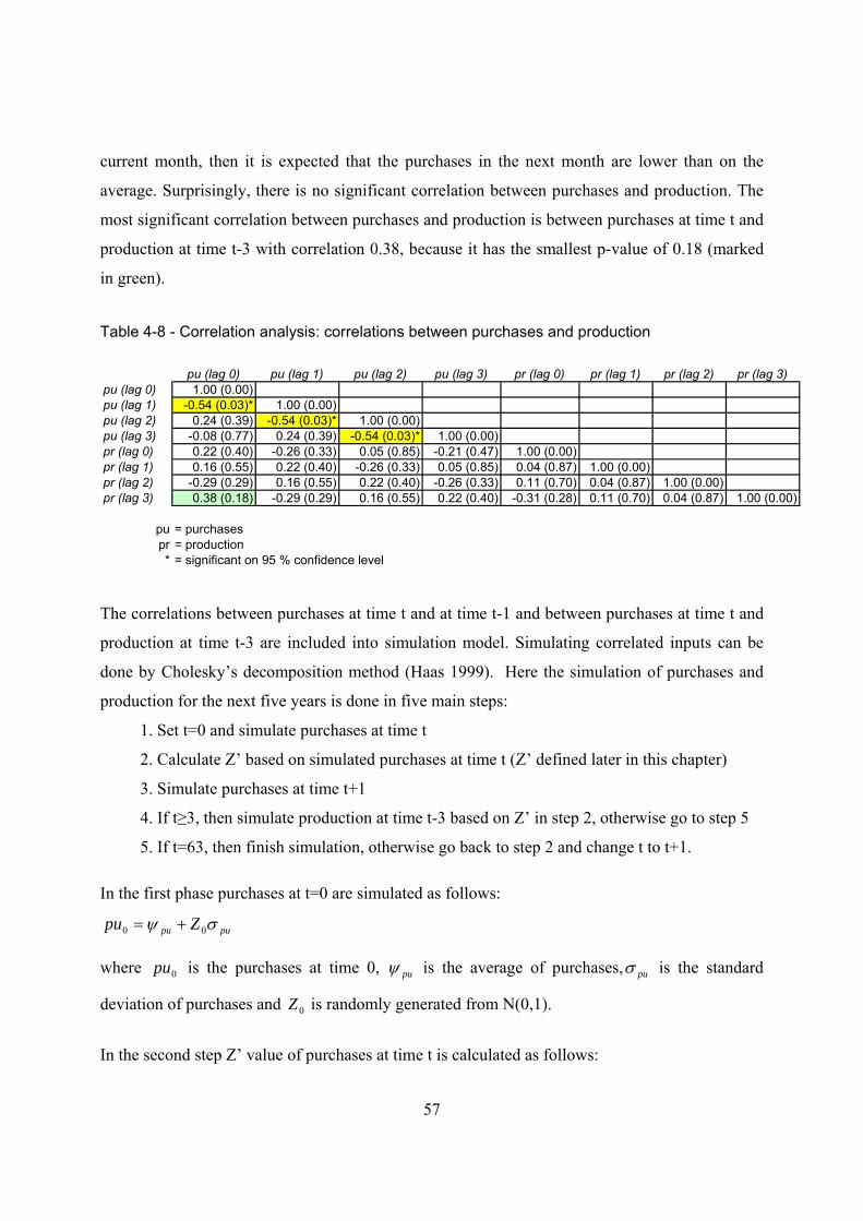
57
current month, then it is expected that the purchases in the next month are lower than on the
average. Surprisingly, there is no significant correlation between purchases and production. The
most significant correlation between purchases and production is between purchases at time t and
production at time t-3 with correlation 0.38, because it has the smallest p-value of 0.18 (marked
in green).
Table 4-8 - Correlation analysis: correlations between purchases and production
pu (lag 0) pu (lag 1) pu (lag 2) pu (lag 3) pr (lag 0) pr (lag 1) pr (lag 2) pr (lag 3)pu (lag 0) 1.00 (0.00)pu (lag 1) -0.54 (0.03)* 1.00 (0.00)pu (lag 2) 0.24 (0.39) -0.54 (0.03)* 1.00 (0.00)pu (lag 3) -0.08 (0.77) 0.24 (0.39) -0.54 (0.03)* 1.00 (0.00)pr (lag 0) 0.22 (0.40) -0.26 (0.33) 0.05 (0.85) -0.21 (0.47) 1.00 (0.00)pr (lag 1) 0.16 (0.55) 0.22 (0.40) -0.26 (0.33) 0.05 (0.85) 0.04 (0.87) 1.00 (0.00)pr (lag 2) -0.29 (0.29) 0.16 (0.55) 0.22 (0.40) -0.26 (0.33) 0.11 (0.70) 0.04 (0.87) 1.00 (0.00)pr (lag 3) 0.38 (0.18) -0.29 (0.29) 0.16 (0.55) 0.22 (0.40) -0.31 (0.28) 0.11 (0.70) 0.04 (0.87) 1.00 (0.00)
pu = purchasespr = production* = significant on 95 % confidence level
The correlations between purchases at time t and at time t-1 and between purchases at time t and
production at time t-3 are included into simulation model. Simulating correlated inputs can be
done by Cholesky’s decomposition method (Haas 1999). Here the simulation of purchases and
production for the next five years is done in five main steps:
1. Set t=0 and simulate purchases at time t
2. Calculate Z’ based on simulated purchases at time t (Z’ defined later in this chapter)
3. Simulate purchases at time t+1
4. If t≥3, then simulate production at time t-3 based on Z’ in step 2, otherwise go to step 5
5. If t=63, then finish simulation, otherwise go back to step 2 and change t to t+1.
In the first phase purchases at t=0 are simulated as follows:
pupu Zpu σψ 00 +=
where 0pu is the purchases at time 0, puψ is the average of purchases, puσ is the standard
deviation of purchases and 0Z is randomly generated from N(0,1).
In the second step Z’ value of purchases at time t is calculated as follows:
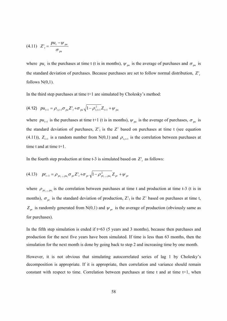
58
(4.11) pu
putt
puZ
σψ−
='
where tpu is the purchases at time t (t is in months), puψ is the average of purchases and puσ is
the standard deviation of purchases. Because purchases are set to follow normal distribution, tZ '
follows N(0,1).
In the third step purchases at time t+1 are simulated by Cholesky’s method:
(4.12) putttputputtt ZZpu ψρσσρ +−+= ++++ 12
1,1,1 1'
where 1+tpu is the purchases at time t+1 (t is in months), puψ is the average of purchases, puσ is
the standard deviation of purchases, Z’t is the Z’ based on purchases at time t (see equation
(4.11)), 1+tZ is a random number from N(0,1) and 1, +ttρ is the correlation between purchases at
time t and at time t+1.
In the fourth step production at time t-3 is simulated based on tZ ' as follows:
(4.13) prprpuprprtprpuprt ZZprtttt
ψρσσρ +−+=−−−
2,,3 33
1'
where tt pupr ,3−
ρ is the correlation between purchases at time t and production at time t-3 (t is in
months), prσ is the standard deviation of production, Z’t is the Z’ based on purchases at time t,
prZ is randomly generated from N(0,1) and prψ is the average of production (obviously same as
for purchases).
In the fifth step simulation is ended if t=63 (5 years and 3 months), because then purchases and
production for the next five years have been simulated. If time is less than 63 months, then the
simulation for the next month is done by going back to step 2 and increasing time by one month.
However, it is not obvious that simulating autocorrelated series of lag 1 by Cholesky’s
decomposition is appropriate. If it is appropriate, then correlation and variance should remain
constant with respect to time. Correlation between purchases at time t and at time t+1, when
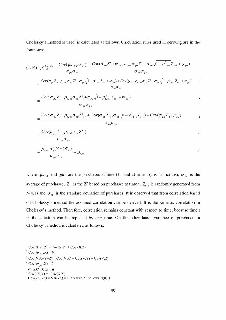
59
Cholesky’s method is used, is calculated as follows. Calculation rules used in deriving are in the
footnotes:
(4.14) pupu
putttputputtputpu
pupu
ttCholeskytt
ZZZCovpupuCovσσ
ψρσσρψσ
σσρ
)1','(),( 12
1,1,11,
+−++== ++++
+
pupu
putttputputtpuputttputputttpu ZZCovZZZCovσσ
ψρσσρψψρσσρσ )1',()1','( 12
1,1,12
1,1, +−+++−+= ++++++ 1
pupu
putttputputttpu ZZZCovσσ
ψρσσρσ )1','( 12
1,1, +−+= +++ 2
pupu
putputttputputputttpu ZCovZZCovZZCovσσ
ψσρσσσρσ ),'()1,'()','( 12
1,1, +−+= +++ 3
pupu
tputttpu ZZCovσσ
σρσ )','( 1, += 4
pupu
tputt ZVarσσ
σρ )'(21, += 1, += ttρ 5
where 1+tpu and tpu are the purchases at time t+1 and at time t (t is in months), puψ is the
average of purchases, tZ ' is the Z’ based on purchases at time t, 1+tZ is randomly generated from
N(0,1) and puσ is the standard deviation of purchases. It is observed that from correlation based
on Cholesky’s method the assumed correlation can be derived. It is the same as correlation in
Cholesky’s method. Therefore, correlation remains constant with respect to time, because time t
in the equation can be replaced by any time. On the other hand, variance of purchases in
Cholesky’s method is calculated as follows:
1 Cov(X,Y+Z) = Cov(X,Y) + Cov (X,Z) 2 Cov( puψ ,X) = 0 3 Cov(V,X+Y+Z) = Cov(V,X) + Cov(V,Y) + Cov(V,Z) 4 Cov( puψ ,X) = 0 Cov(Z’t, Zt+1) = 0 5 Cov(aX,Y) = aCov(X,Y) Cov(Z’t, Z’t) = Var(Z’t) = 1, because Z’t follows N(0,1)
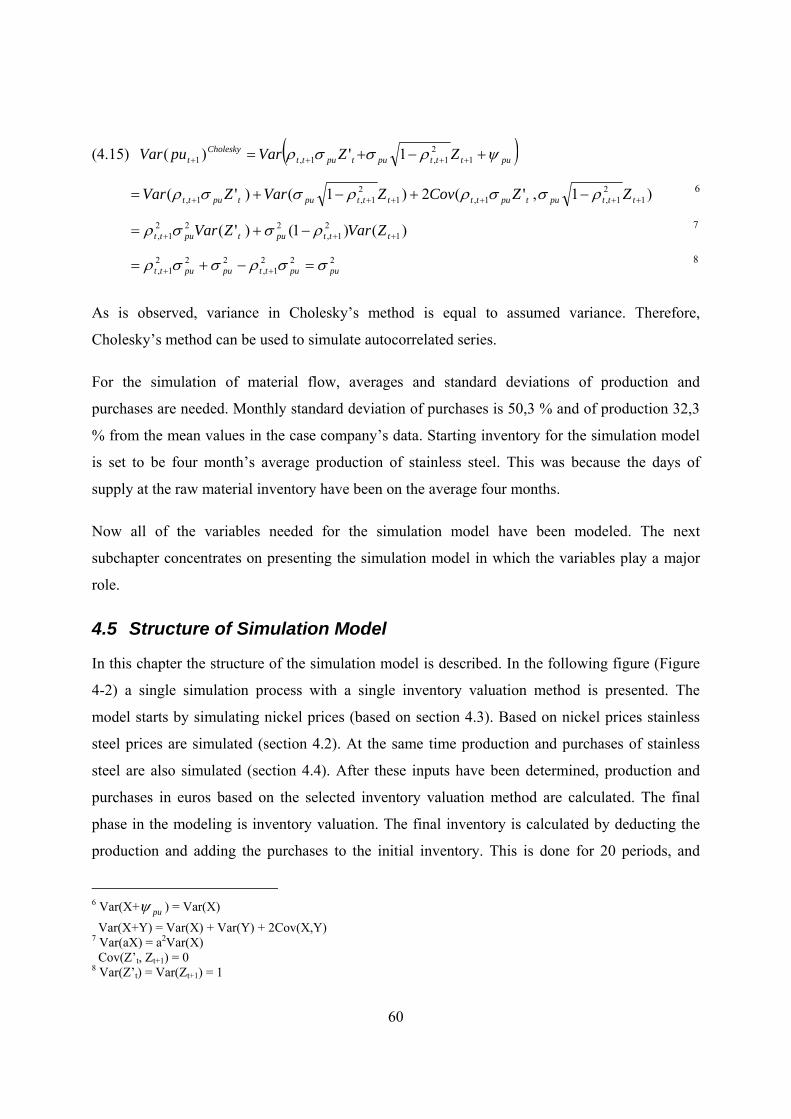
60
(4.15) ( )putttputputtCholesky
t ZZVarpuVar ψρσσρ +−+= ++++ 12
1,1,1 1')(
)1,'(2)1()'( 12
1,1,12
1,1, ++++++ −+−+= tttputputttttputputt ZZCovZVarZVar ρσσρρσσρ 6
)()1()'( 12
1,222
1, +++ −+= tttputputt ZVarZVar ρσσρ 7
2221,
2221, puputtpuputt σσρσσρ =−+= ++ 8
As is observed, variance in Cholesky’s method is equal to assumed variance. Therefore,
Cholesky’s method can be used to simulate autocorrelated series.
For the simulation of material flow, averages and standard deviations of production and
purchases are needed. Monthly standard deviation of purchases is 50,3 % and of production 32,3
% from the mean values in the case company’s data. Starting inventory for the simulation model
is set to be four month’s average production of stainless steel. This was because the days of
supply at the raw material inventory have been on the average four months.
Now all of the variables needed for the simulation model have been modeled. The next
subchapter concentrates on presenting the simulation model in which the variables play a major
role.
4.5 Structure of Simulation Model
In this chapter the structure of the simulation model is described. In the following figure (Figure
4-2) a single simulation process with a single inventory valuation method is presented. The
model starts by simulating nickel prices (based on section 4.3). Based on nickel prices stainless
steel prices are simulated (section 4.2). At the same time production and purchases of stainless
steel are also simulated (section 4.4). After these inputs have been determined, production and
purchases in euros based on the selected inventory valuation method are calculated. The final
phase in the modeling is inventory valuation. The final inventory is calculated by deducting the
production and adding the purchases to the initial inventory. This is done for 20 periods, and
6 Var(X+ puψ ) = Var(X) Var(X+Y) = Var(X) + Var(Y) + 2Cov(X,Y) 7 Var(aX) = a2Var(X) Cov(Z’t, Zt+1) = 0 8 Var(Z’t) = Var(Zt+1) = 1
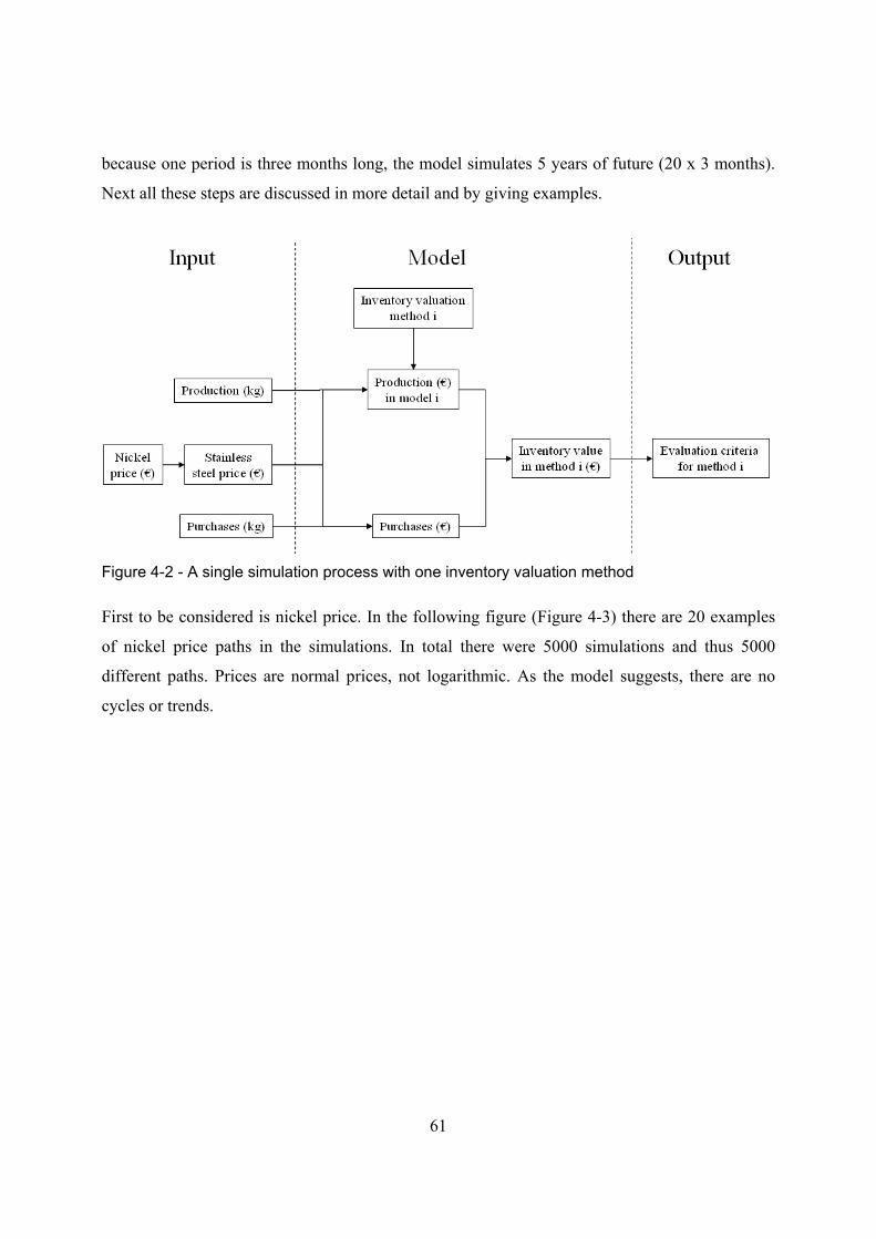
61
because one period is three months long, the model simulates 5 years of future (20 x 3 months).
Next all these steps are discussed in more detail and by giving examples.
Figure 4-2 - A single simulation process with one inventory valuation method
First to be considered is nickel price. In the following figure (Figure 4-3) there are 20 examples
of nickel price paths in the simulations. In total there were 5000 simulations and thus 5000
different paths. Prices are normal prices, not logarithmic. As the model suggests, there are no
cycles or trends.
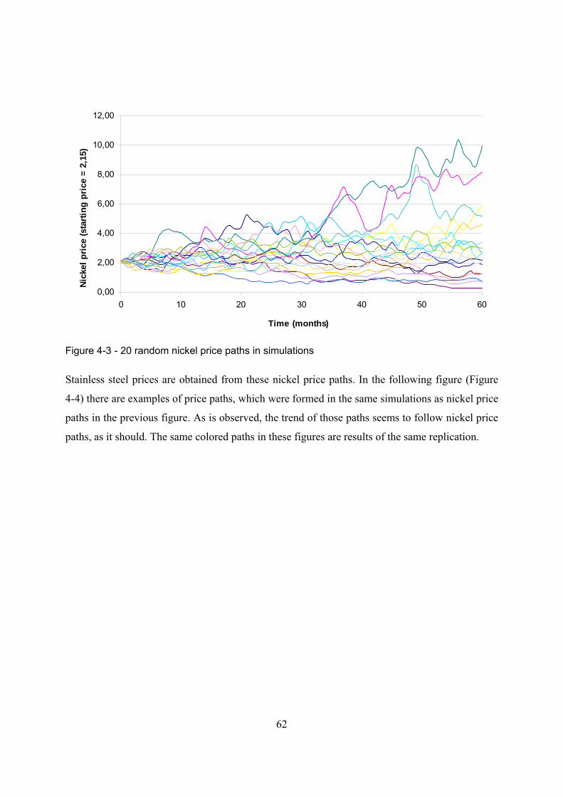
62
0,00
2,00
4,00
6,00
8,00
10,00
12,00
0 10 20 30 40 50 60
Time (months)
Nic
kel p
rice
(sta
rtin
g pr
ice
= 2,
15)
Figure 4-3 - 20 random nickel price paths in simulations
Stainless steel prices are obtained from these nickel price paths. In the following figure (Figure
4-4) there are examples of price paths, which were formed in the same simulations as nickel price
paths in the previous figure. As is observed, the trend of those paths seems to follow nickel price
paths, as it should. The same colored paths in these figures are results of the same replication.
63
0,00
2,00
4,00
6,00
8,00
10,00
12,00
0 10 20 30 40 50 60
Time (months)
Stai
nles
s st
eel p
rice
(sta
rting
pri
ce =
3,0
0)
Figure 4-4 - 20 random stainless steel price paths in simulations
In order to form inventory values by different inventory valuation methods, purchases and
production in kilograms have to be simulated. Purchases and production in the next five years
were simulated 5000 times, and in the following figure (Figure 4-5) there is an example of a
simulated path of purchases, production and inventory in kilograms.
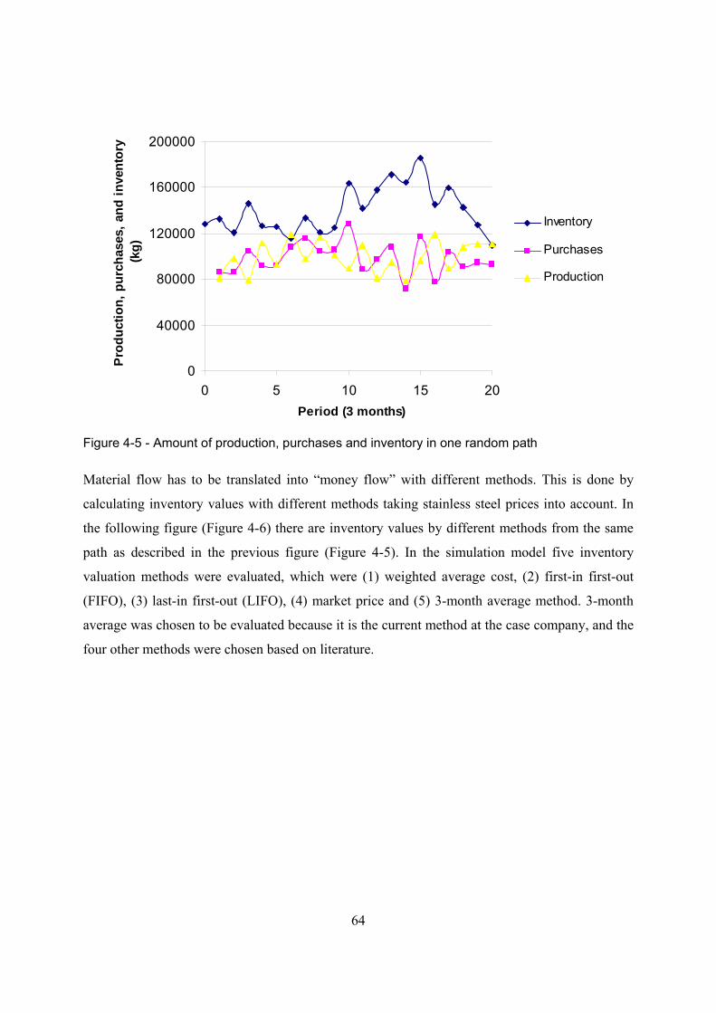
64
0
40000
80000
120000
160000
200000
0 5 10 15 20Period (3 months)
Pro
duct
ion,
pur
chas
es, a
nd in
vent
ory
(kg)
Inventory
Purchases
Production
Figure 4-5 - Amount of production, purchases and inventory in one random path
Material flow has to be translated into “money flow” with different methods. This is done by
calculating inventory values with different methods taking stainless steel prices into account. In
the following figure (Figure 4-6) there are inventory values by different methods from the same
path as described in the previous figure (Figure 4-5). In the simulation model five inventory
valuation methods were evaluated, which were (1) weighted average cost, (2) first-in first-out
(FIFO), (3) last-in first-out (LIFO), (4) market price and (5) 3-month average method. 3-month
average was chosen to be evaluated because it is the current method at the case company, and the
four other methods were chosen based on literature.
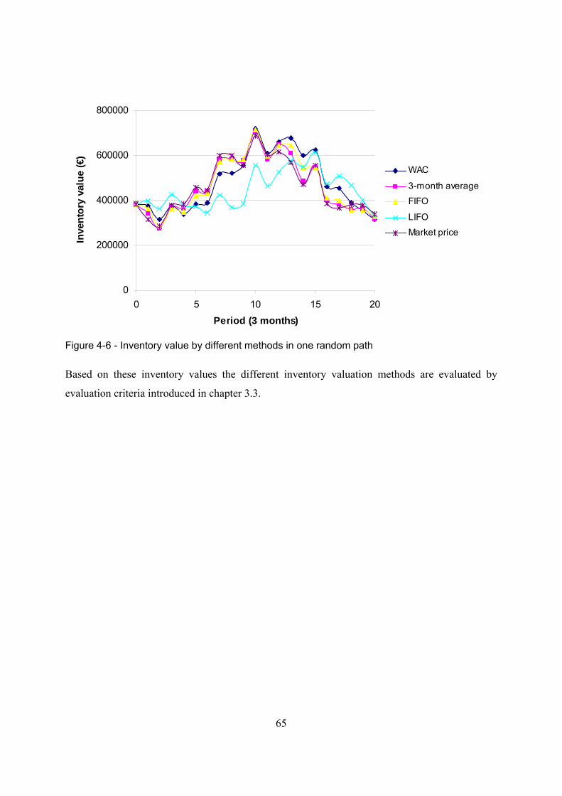
65
0
200000
400000
600000
800000
0 5 10 15 20Period (3 months)
Inve
ntor
y va
lue
(€)
WAC
3-month average
FIFO
LIFO
Market price
Figure 4-6 - Inventory value by different methods in one random path
Based on these inventory values the different inventory valuation methods are evaluated by
evaluation criteria introduced in chapter 3.3.
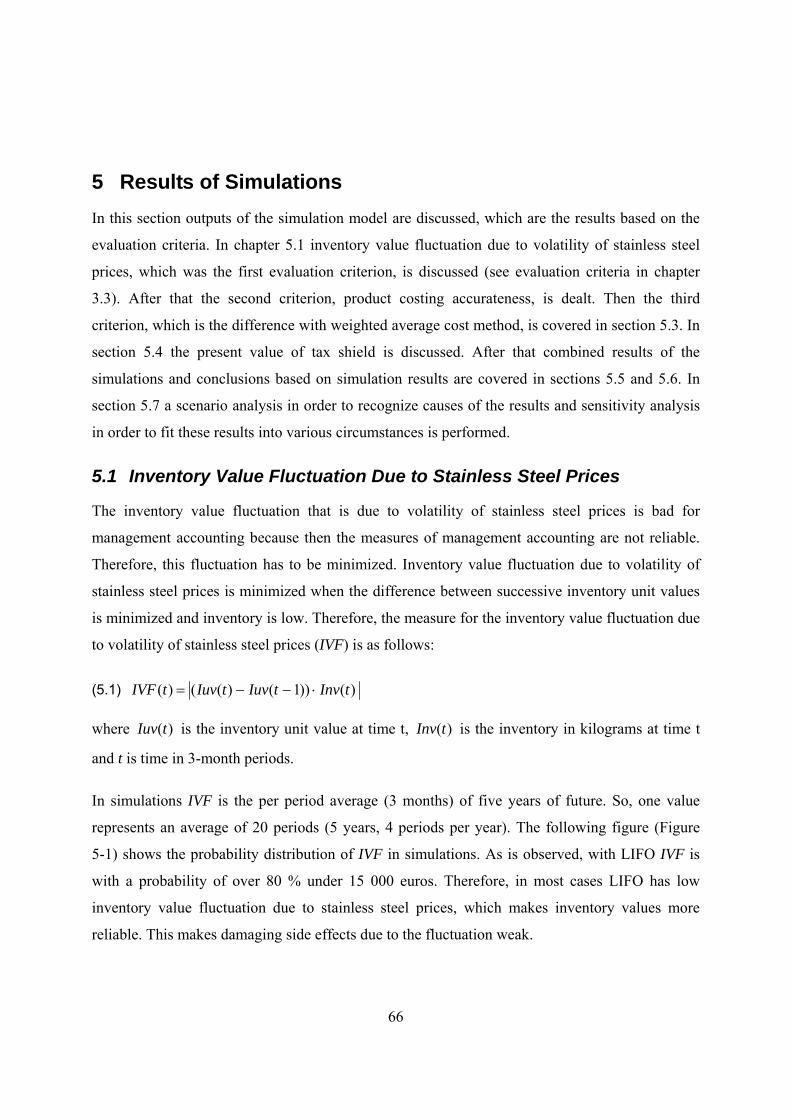
66
5 Results of Simulations In this section outputs of the simulation model are discussed, which are the results based on the
evaluation criteria. In chapter 5.1 inventory value fluctuation due to volatility of stainless steel
prices, which was the first evaluation criterion, is discussed (see evaluation criteria in chapter
3.3). After that the second criterion, product costing accurateness, is dealt. Then the third
criterion, which is the difference with weighted average cost method, is covered in section 5.3. In
section 5.4 the present value of tax shield is discussed. After that combined results of the
simulations and conclusions based on simulation results are covered in sections 5.5 and 5.6. In
section 5.7 a scenario analysis in order to recognize causes of the results and sensitivity analysis
in order to fit these results into various circumstances is performed.
5.1 Inventory Value Fluctuation Due to Stainless Steel Prices
The inventory value fluctuation that is due to volatility of stainless steel prices is bad for
management accounting because then the measures of management accounting are not reliable.
Therefore, this fluctuation has to be minimized. Inventory value fluctuation due to volatility of
stainless steel prices is minimized when the difference between successive inventory unit values
is minimized and inventory is low. Therefore, the measure for the inventory value fluctuation due
to volatility of stainless steel prices (IVF) is as follows:
(5.1) )())1()(()( tInvtIuvtIuvtIVF ⋅−−=
where )(tIuv is the inventory unit value at time t, )(tInv is the inventory in kilograms at time t
and t is time in 3-month periods.
In simulations IVF is the per period average (3 months) of five years of future. So, one value
represents an average of 20 periods (5 years, 4 periods per year). The following figure (Figure
5-1) shows the probability distribution of IVF in simulations. As is observed, with LIFO IVF is
with a probability of over 80 % under 15 000 euros. Therefore, in most cases LIFO has low
inventory value fluctuation due to stainless steel prices, which makes inventory values more
reliable. This makes damaging side effects due to the fluctuation weak.
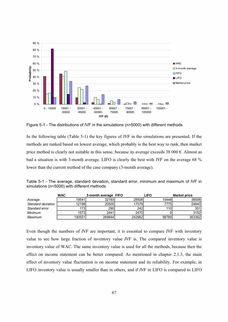
67
0 %
10 %
20 %
30 %
40 %
50 %
60 %
70 %
80 %
90 %
0 - 15000 15001 -30000
30001 -45000
45001 -60000
60001 -75000
75001 -90000
90001 -105000
105001 -
IVF (€)
Pro
babi
lity
WAC
3-month average
FIFO
LIFO
Market price
Figure 5-1 - The distributions of IVF in the simulations (n=5000) with different methods
In the following table (Table 5-1) the key figures of IVF in the simulations are presented. If the
methods are ranked based on lowest average, which probably is the best way to rank, then market
price method is clearly not suitable in this sense, because its average exceeds 38 000 €. Almost as
bad a situation is with 3-month average. LIFO is clearly the best with IVF on the average 68 %
lower than the current method of the case company (3-month average).
Table 5-1 - The average, standard deviation, standard error, minimum and maximum of IVF in simulations (n=5000) with different methods
WAC 3-month average FIFO LIFO Market priceAverage 19541 32193 28508 10448 38508Standard deviation 12198 20500 17079 7775 24840Standard error 173 290 242 110 351Minimum 1573 2441 2470 0 3152Maximum 190551 269844 242962 98789 363362
Even though the numbers of IVF are important, it is essential to compare IVF with inventory
value to see how large fraction of inventory value IVF is. The compared inventory value is
inventory value of WAC. The same inventory value is used for all the methods, because then the
effect on income statement can be better compared. As mentioned in chapter 2.1.3, the main
effect of inventory value fluctuation is on income statement and its reliability. For example, in
LIFO inventory value is usually smaller than in others, and if IVF in LIFO is compared to LIFO
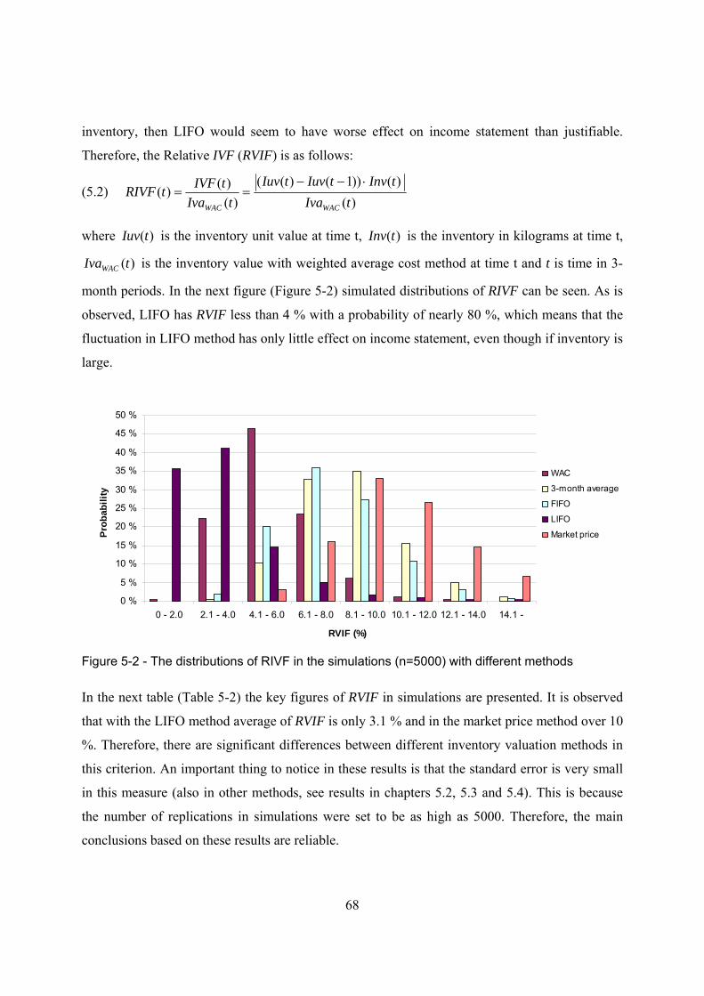
68
inventory, then LIFO would seem to have worse effect on income statement than justifiable.
Therefore, the Relative IVF (RVIF) is as follows:
(5.2) )(
)())1()(()(
)()(tIva
tInvtIuvtIuvtIva
tIVFtRIVFWACWAC
⋅−−==
where )(tIuv is the inventory unit value at time t, )(tInv is the inventory in kilograms at time t,
)(tIvaWAC is the inventory value with weighted average cost method at time t and t is time in 3-
month periods. In the next figure (Figure 5-2) simulated distributions of RIVF can be seen. As is
observed, LIFO has RVIF less than 4 % with a probability of nearly 80 %, which means that the
fluctuation in LIFO method has only little effect on income statement, even though if inventory is
large.
0 %
5 %
10 %
15 %
20 %
25 %
30 %
35 %
40 %
45 %
50 %
0 - 2.0 2.1 - 4.0 4.1 - 6.0 6.1 - 8.0 8.1 - 10.0 10.1 - 12.0 12.1 - 14.0 14.1 -
RVIF (%)
Pro
babi
lity
WAC
3-month average
FIFO
LIFO
Market price
Figure 5-2 - The distributions of RIVF in the simulations (n=5000) with different methods
In the next table (Table 5-2) the key figures of RVIF in simulations are presented. It is observed
that with the LIFO method average of RVIF is only 3.1 % and in the market price method over 10
%. Therefore, there are significant differences between different inventory valuation methods in
this criterion. An important thing to notice in these results is that the standard error is very small
in this measure (also in other methods, see results in chapters 5.2, 5.3 and 5.4). This is because
the number of replications in simulations were set to be as high as 5000. Therefore, the main
conclusions based on these results are reliable.
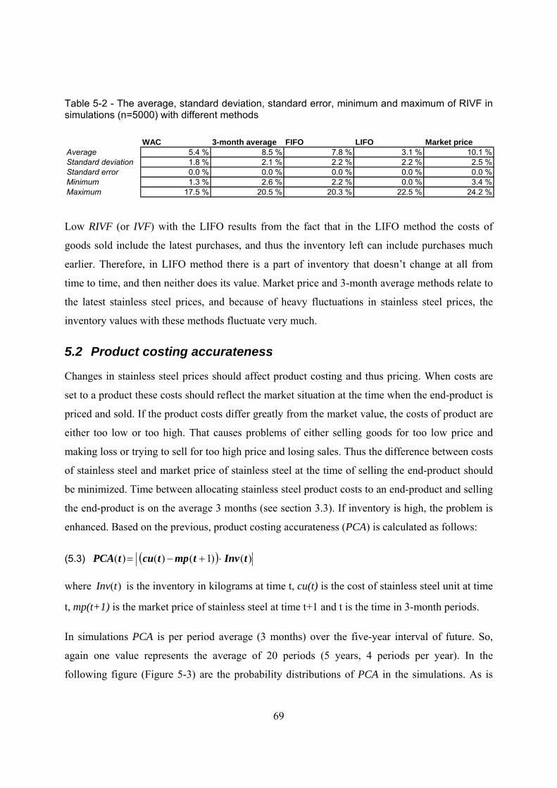
69
Table 5-2 - The average, standard deviation, standard error, minimum and maximum of RIVF in simulations (n=5000) with different methods
WAC 3-month average FIFO LIFO Market priceAverage 5.4 % 8.5 % 7.8 % 3.1 % 10.1 %Standard deviation 1.8 % 2.1 % 2.2 % 2.2 % 2.5 %Standard error 0.0 % 0.0 % 0.0 % 0.0 % 0.0 %Minimum 1.3 % 2.6 % 2.2 % 0.0 % 3.4 %Maximum 17.5 % 20.5 % 20.3 % 22.5 % 24.2 %
Low RIVF (or IVF) with the LIFO results from the fact that in the LIFO method the costs of
goods sold include the latest purchases, and thus the inventory left can include purchases much
earlier. Therefore, in LIFO method there is a part of inventory that doesn’t change at all from
time to time, and then neither does its value. Market price and 3-month average methods relate to
the latest stainless steel prices, and because of heavy fluctuations in stainless steel prices, the
inventory values with these methods fluctuate very much.
5.2 Product costing accurateness
Changes in stainless steel prices should affect product costing and thus pricing. When costs are
set to a product these costs should reflect the market situation at the time when the end-product is
priced and sold. If the product costs differ greatly from the market value, the costs of product are
either too low or too high. That causes problems of either selling goods for too low price and
making loss or trying to sell for too high price and losing sales. Thus the difference between costs
of stainless steel and market price of stainless steel at the time of selling the end-product should
be minimized. Time between allocating stainless steel product costs to an end-product and selling
the end-product is on the average 3 months (see section 3.3). If inventory is high, the problem is
enhanced. Based on the previous, product costing accurateness (PCA) is calculated as follows:
(5.3) ( ) )()1()()( tInvtmptcutPCA ⋅+−=
where )(tInv is the inventory in kilograms at time t, cu(t) is the cost of stainless steel unit at time
t, mp(t+1) is the market price of stainless steel at time t+1 and t is the time in 3-month periods.
In simulations PCA is per period average (3 months) over the five-year interval of future. So,
again one value represents the average of 20 periods (5 years, 4 periods per year). In the
following figure (Figure 5-3) are the probability distributions of PCA in the simulations. As is
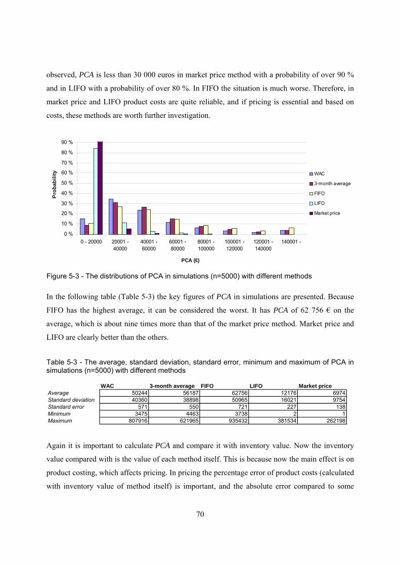
70
observed, PCA is less than 30 000 euros in market price method with a probability of over 90 %
and in LIFO with a probability of over 80 %. In FIFO the situation is much worse. Therefore, in
market price and LIFO product costs are quite reliable, and if pricing is essential and based on
costs, these methods are worth further investigation.
0 %
10 %
20 %
30 %
40 %
50 %
60 %
70 %
80 %
90 %
0 - 20000 20001 -40000
40001 -60000
60001 -80000
80001 -100000
100001 -120000
120001 -140000
140001 -
PCA (€)
Pro
babi
lity WAC
3-month average
FIFO
LIFO
Market price
Figure 5-3 - The distributions of PCA in simulations (n=5000) with different methods
In the following table (Table 5-3) the key figures of PCA in simulations are presented. Because
FIFO has the highest average, it can be considered the worst. It has PCA of 62 756 € on the
average, which is about nine times more than that of the market price method. Market price and
LIFO are clearly better than the others.
Table 5-3 - The average, standard deviation, standard error, minimum and maximum of PCA in simulations (n=5000) with different methods
WAC 3-month average FIFO LIFO Market priceAverage 50244 56187 62756 12176 6974Standard deviation 40360 38898 50965 16021 9754Standard error 571 550 721 227 138Minimum 3475 4463 3738 2 1Maximum 807916 621965 935432 381534 262198
Again it is important to calculate PCA and compare it with inventory value. Now the inventory
value compared with is the value of each method itself. This is because now the main effect is on
product costing, which affects pricing. In pricing the percentage error of product costs (calculated
with inventory value of method itself) is important, and the absolute error compared to some
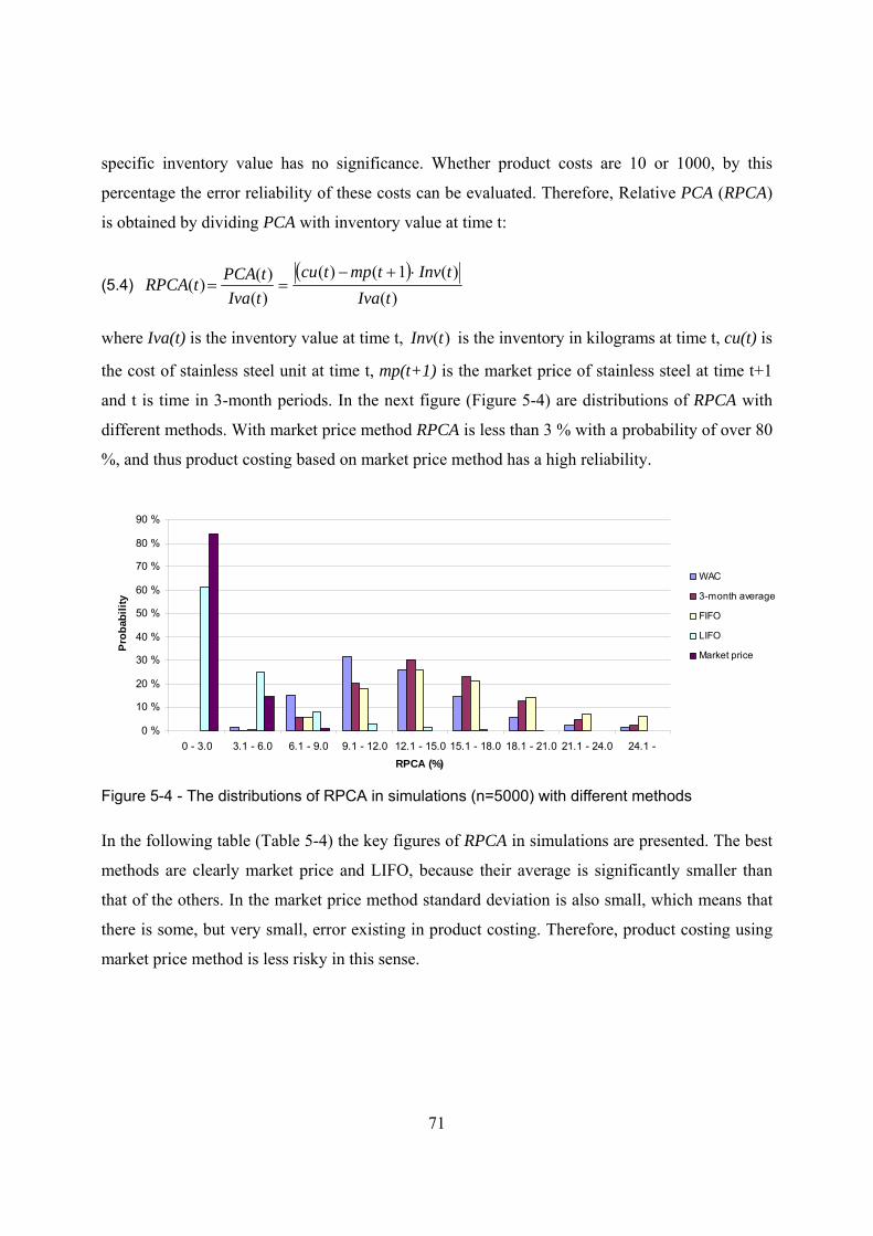
71
specific inventory value has no significance. Whether product costs are 10 or 1000, by this
percentage the error reliability of these costs can be evaluated. Therefore, Relative PCA (RPCA)
is obtained by dividing PCA with inventory value at time t:
(5.4) ( )
)()(1()(
)()()(
tIvatInvtmptcu
tIvatPCAtRPCA
⋅+−==
where Iva(t) is the inventory value at time t, )(tInv is the inventory in kilograms at time t, cu(t) is
the cost of stainless steel unit at time t, mp(t+1) is the market price of stainless steel at time t+1
and t is time in 3-month periods. In the next figure (Figure 5-4) are distributions of RPCA with
different methods. With market price method RPCA is less than 3 % with a probability of over 80
%, and thus product costing based on market price method has a high reliability.
0 %
10 %
20 %
30 %
40 %
50 %
60 %
70 %
80 %
90 %
0 - 3.0 3.1 - 6.0 6.1 - 9.0 9.1 - 12.0 12.1 - 15.0 15.1 - 18.0 18.1 - 21.0 21.1 - 24.0 24.1 - RPCA (%)
Pro
babi
lity
WAC
3-month average
FIFO
LIFO
Market price
Figure 5-4 - The distributions of RPCA in simulations (n=5000) with different methods
In the following table (Table 5-4) the key figures of RPCA in simulations are presented. The best
methods are clearly market price and LIFO, because their average is significantly smaller than
that of the others. In the market price method standard deviation is also small, which means that
there is some, but very small, error existing in product costing. Therefore, product costing using
market price method is less risky in this sense.
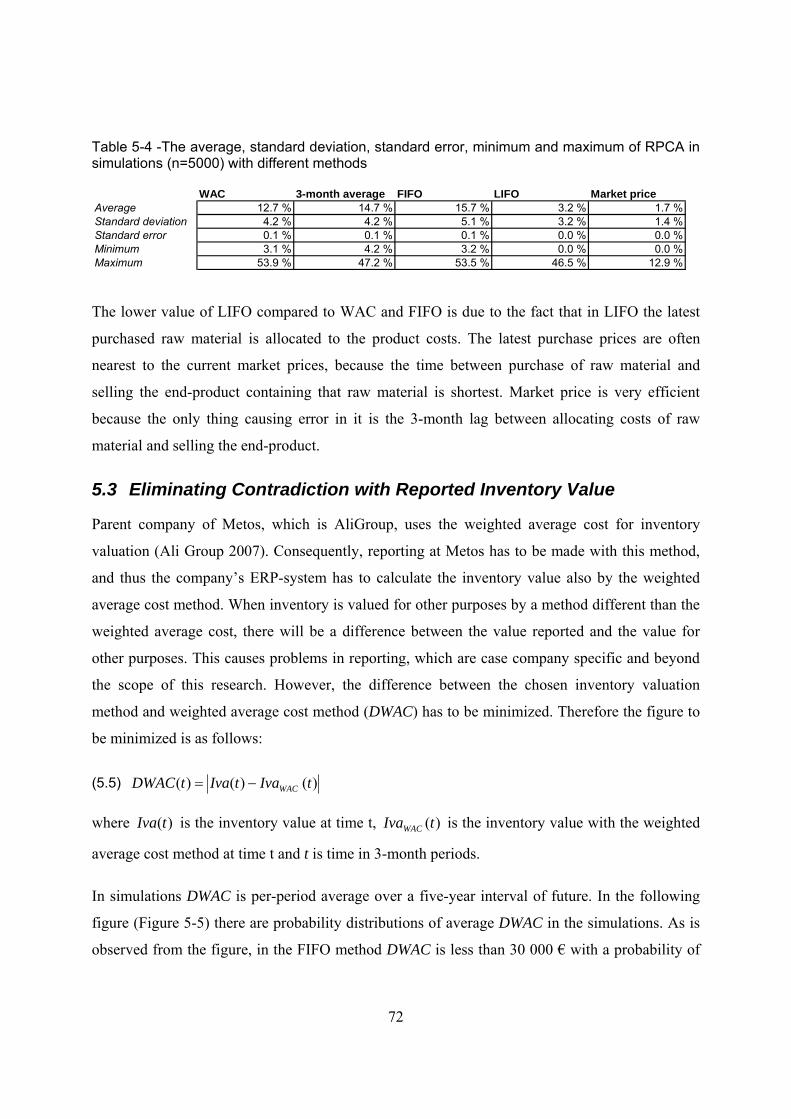
72
Table 5-4 -The average, standard deviation, standard error, minimum and maximum of RPCA in simulations (n=5000) with different methods
WAC 3-month average FIFO LIFO Market priceAverage 12.7 % 14.7 % 15.7 % 3.2 % 1.7 %Standard deviation 4.2 % 4.2 % 5.1 % 3.2 % 1.4 %Standard error 0.1 % 0.1 % 0.1 % 0.0 % 0.0 %Minimum 3.1 % 4.2 % 3.2 % 0.0 % 0.0 %Maximum 53.9 % 47.2 % 53.5 % 46.5 % 12.9 %
The lower value of LIFO compared to WAC and FIFO is due to the fact that in LIFO the latest
purchased raw material is allocated to the product costs. The latest purchase prices are often
nearest to the current market prices, because the time between purchase of raw material and
selling the end-product containing that raw material is shortest. Market price is very efficient
because the only thing causing error in it is the 3-month lag between allocating costs of raw
material and selling the end-product.
5.3 Eliminating Contradiction with Reported Inventory Value
Parent company of Metos, which is AliGroup, uses the weighted average cost for inventory
valuation (Ali Group 2007). Consequently, reporting at Metos has to be made with this method,
and thus the company’s ERP-system has to calculate the inventory value also by the weighted
average cost method. When inventory is valued for other purposes by a method different than the
weighted average cost, there will be a difference between the value reported and the value for
other purposes. This causes problems in reporting, which are case company specific and beyond
the scope of this research. However, the difference between the chosen inventory valuation
method and weighted average cost method (DWAC) has to be minimized. Therefore the figure to
be minimized is as follows:
(5.5) )()()( tIvatIvatDWAC WAC−=
where )(tIva is the inventory value at time t, )(tIvaWAC is the inventory value with the weighted
average cost method at time t and t is time in 3-month periods.
In simulations DWAC is per-period average over a five-year interval of future. In the following
figure (Figure 5-5) there are probability distributions of average DWAC in the simulations. As is
observed from the figure, in the FIFO method DWAC is less than 30 000 € with a probability of
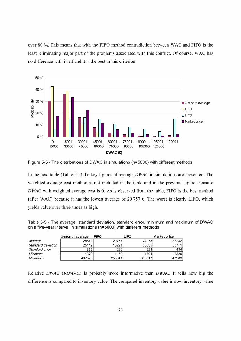
73
over 80 %. This means that with the FIFO method contradiction between WAC and FIFO is the
least, eliminating major part of the problems associated with this conflict. Of course, WAC has
no difference with itself and it is the best in this criterion.
0 %
10 %
20 %
30 %
40 %
50 %
0 -15000
15001 -30000
30001 -45000
45001 -60000
60001 -75000
75001 -90000
90001 -105000
105001 -120000
120001 -
DWAC (€)
Prob
abili
ty 3-month average
FIFO
LIFO
Market price
Figure 5-5 - The distributions of DWAC in simulations (n=5000) with different methods
In the next table (Table 5-5) the key figures of average DWAC in simulations are presented. The
weighted average cost method is not included in the table and in the previous figure, because
DWAC with weighted average cost is 0. As is observed from the table, FIFO is the best method
(after WAC) because it has the lowest average of 20 757 €. The worst is clearly LIFO, which
yields value over three times as high.
Table 5-5 - The average, standard deviation, standard error, minimum and maximum of DWAC on a five-year interval in simulations (n=5000) with different methods
3-month average FIFO LIFO Market priceAverage 28542 20757 74078 37242Standard deviation 25112 16221 65635 30711Standard error 355 229 928 434Minimum 1379 1170 1304 2320Maximum 407573 255341 688817 547283
Relative DWAC (RDWAC) is probably more informative than DWAC. It tells how big the
difference is compared to inventory value. The compared inventory value is now inventory value
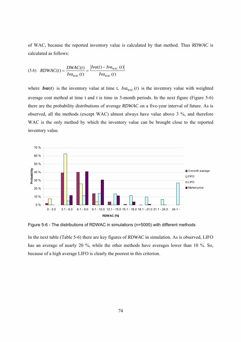
74
of WAC, because the reported inventory value is calculated by that method. Thus RDWAC is
calculated as follows:
(5.6) )(
)()()()()(
tIvatIvatIva
tIvatDWACtRDWAC
WAC
WAC
WAC
−==
where )(tIva is the inventory value at time t, )(tIvaWAC is the inventory value with weighted
average cost method at time t and t is time in 3-month periods. In the next figure (Figure 5-6)
there are the probability distributions of average RDWAC on a five-year interval of future. As is
observed, all the methods (except WAC) almost always have value above 3 %, and therefore
WAC is the only method by which the inventory value can be brought close to the reported
inventory value.
0 %
10 %
20 %
30 %
40 %
50 %
60 %
70 %
0 - 3.0 3.1 - 6.0 6.1 - 9.0 9.1 - 12.0 12.1 - 15.0 15.1 - 18.0 18.1 - 21.0 21.1 - 24.0 24.1 -
RDWAC (%)
Prob
abili
ty 3-month average
FIFO
LIFO
Market price
Figure 5-6 - The distributions of RDWAC in simulations (n=5000) with different methods
In the next table (Table 5-6) there are key figures of RDWAC in simulation. As is observed, LIFO
has an average of nearly 20 %, while the other methods have averages lower than 10 %. So,
because of a high average LIFO is clearly the poorest in this criterion.
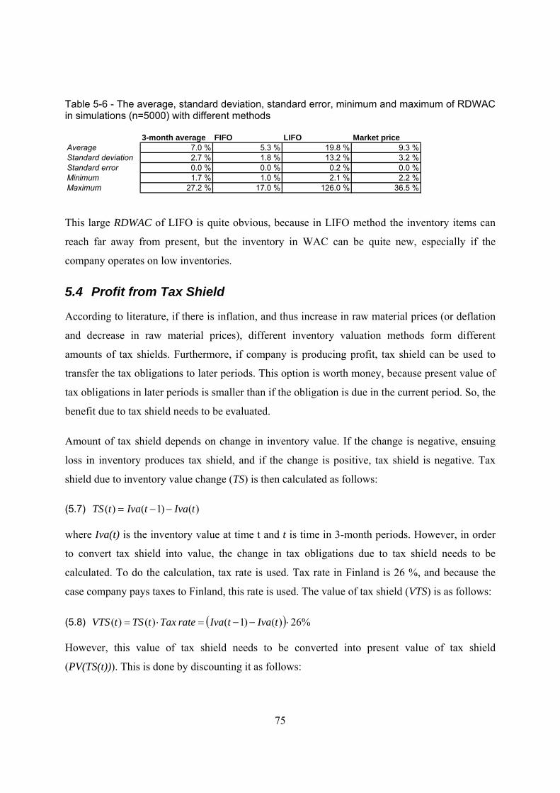
75
Table 5-6 - The average, standard deviation, standard error, minimum and maximum of RDWAC in simulations (n=5000) with different methods
3-month average FIFO LIFO Market priceAverage 7.0 % 5.3 % 19.8 % 9.3 %Standard deviation 2.7 % 1.8 % 13.2 % 3.2 %Standard error 0.0 % 0.0 % 0.2 % 0.0 %Minimum 1.7 % 1.0 % 2.1 % 2.2 %Maximum 27.2 % 17.0 % 126.0 % 36.5 %
This large RDWAC of LIFO is quite obvious, because in LIFO method the inventory items can
reach far away from present, but the inventory in WAC can be quite new, especially if the
company operates on low inventories.
5.4 Profit from Tax Shield
According to literature, if there is inflation, and thus increase in raw material prices (or deflation
and decrease in raw material prices), different inventory valuation methods form different
amounts of tax shields. Furthermore, if company is producing profit, tax shield can be used to
transfer the tax obligations to later periods. This option is worth money, because present value of
tax obligations in later periods is smaller than if the obligation is due in the current period. So, the
benefit due to tax shield needs to be evaluated.
Amount of tax shield depends on change in inventory value. If the change is negative, ensuing
loss in inventory produces tax shield, and if the change is positive, tax shield is negative. Tax
shield due to inventory value change (TS) is then calculated as follows:
(5.7) )()1()( tIvatIvatTS −−=
where Iva(t) is the inventory value at time t and t is time in 3-month periods. However, in order
to convert tax shield into value, the change in tax obligations due to tax shield needs to be
calculated. To do the calculation, tax rate is used. Tax rate in Finland is 26 %, and because the
case company pays taxes to Finland, this rate is used. The value of tax shield (VTS) is as follows:
(5.8) ( ) %26)()1()()( ⋅−−=⋅= tIvatIvarateTaxtTStVTS
However, this value of tax shield needs to be converted into present value of tax shield
(PV(TS(t))). This is done by discounting it as follows:
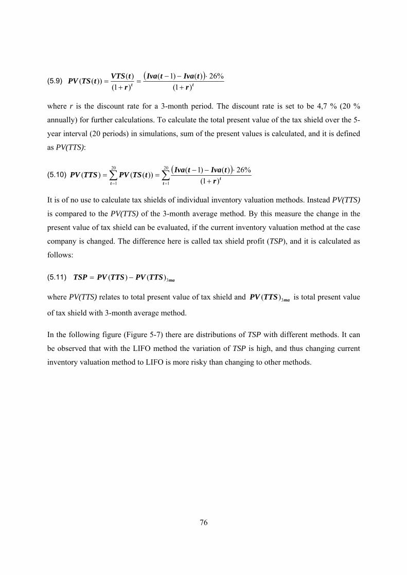
76
(5.9) ( )tt r
tIvatIvartVTStTSPV
)1(%26)()1(
)1()())((
+⋅−−
=+
=
where r is the discount rate for a 3-month period. The discount rate is set to be 4,7 % (20 %
annually) for further calculations. To calculate the total present value of the tax shield over the 5-
year interval (20 periods) in simulations, sum of the present values is calculated, and it is defined
as PV(TTS):
(5.10) ( )∑∑== +
⋅−−==
20
1
20
1 )1(%26)()1())(()(
tt
t rtIvatIvatTSPVTTSPV
It is of no use to calculate tax shields of individual inventory valuation methods. Instead PV(TTS)
is compared to the PV(TTS) of the 3-month average method. By this measure the change in the
present value of tax shield can be evaluated, if the current inventory valuation method at the case
company is changed. The difference here is called tax shield profit (TSP), and it is calculated as
follows:
(5.11) maTTSPVTTSPVTSP 3)()( −=
where PV(TTS) relates to total present value of tax shield and maTTSPV 3)( is total present value
of tax shield with 3-month average method.
In the following figure (Figure 5-7) there are distributions of TSP with different methods. It can
be observed that with the LIFO method the variation of TSP is high, and thus changing current
inventory valuation method to LIFO is more risky than changing to other methods.
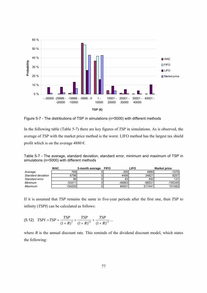
77
0 %
10 %
20 %
30 %
40 %
50 %
60 %
- -30000 -29999 --20000
-19999 --10000
-9999 - 0 1 -10000
10001 -20000
20001 -30000
30001 -40000
40001 -
TSP (€)
Pro
babi
lity WAC
FIFO
LIFO
Market price
Figure 5-7 - The distributions of TSP in simulations (n=5000) with different methods
In the following table (Table 5-7) there are key figures of TSP in simulations. As is observed, the
average of TSP with the market price method is the worst. LIFO method has the largest tax shield
profit which is on the average 4880 €.
Table 5-7 - The average, standard deviation, standard error, minimum and maximum of TSP in simulations (n=5000) with different methods
WAC 3-month average FIFO LIFO Market priceAverage 769 0 -305 4880 -1075Standard deviation 6796 0 4456 34821 9257Standard error 96 0 63 492 131Minimum -53411 0 -46863 -98531 -155345Maximum 154255 0 84931 517441 101483
If it is assumed that TSP remains the same in five-year periods after the first one, then TSP to
infinity (TSPI) can be calculated as follows:
(5.12) ...)1()1()1( 15105 R
TSPR
TSPR
TSPTSPTSPI+
++
++
+=
where R is the annual discount rate. This reminds of the dividend discount model, which states
the following:
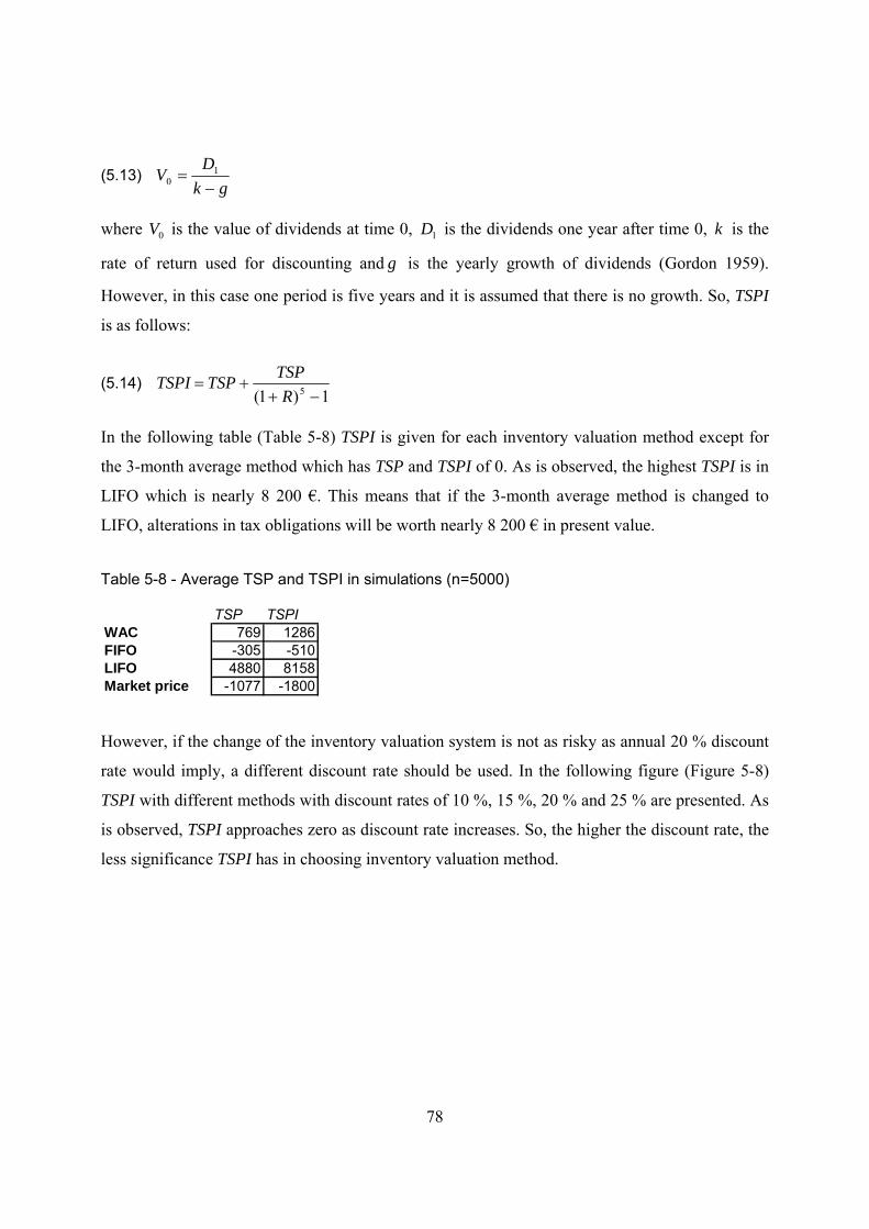
78
(5.13) gk
DV
−= 1
0
where 0V is the value of dividends at time 0, 1D is the dividends one year after time 0, k is the
rate of return used for discounting and g is the yearly growth of dividends (Gordon 1959).
However, in this case one period is five years and it is assumed that there is no growth. So, TSPI
is as follows:
(5.14) 1)1( 5 −+
+=R
TSPTSPTSPI
In the following table (Table 5-8) TSPI is given for each inventory valuation method except for
the 3-month average method which has TSP and TSPI of 0. As is observed, the highest TSPI is in
LIFO which is nearly 8 200 €. This means that if the 3-month average method is changed to
LIFO, alterations in tax obligations will be worth nearly 8 200 € in present value.
Table 5-8 - Average TSP and TSPI in simulations (n=5000)
TSP TSPIWAC 769 1286FIFO -305 -510LIFO 4880 8158Market price -1077 -1800
However, if the change of the inventory valuation system is not as risky as annual 20 % discount
rate would imply, a different discount rate should be used. In the following figure (Figure 5-8)
TSPI with different methods with discount rates of 10 %, 15 %, 20 % and 25 % are presented. As
is observed, TSPI approaches zero as discount rate increases. So, the higher the discount rate, the
less significance TSPI has in choosing inventory valuation method.
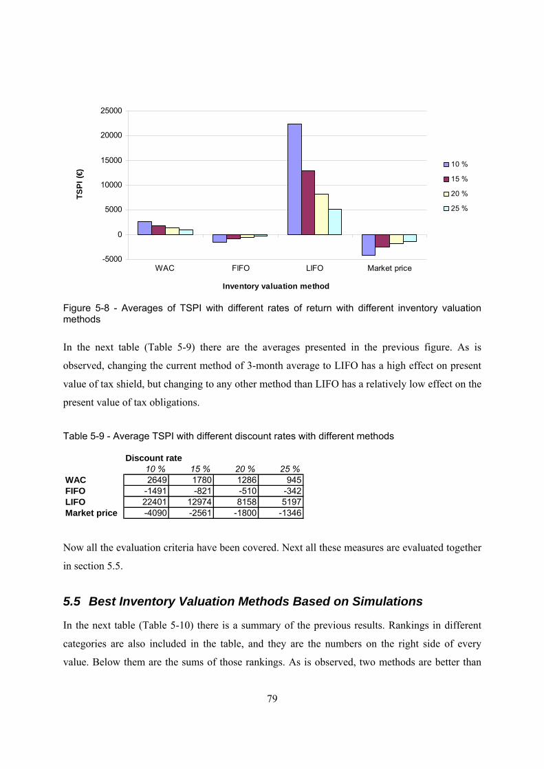
79
-5000
0
5000
10000
15000
20000
25000
WAC FIFO LIFO Market price
Inventory valuation method
TSP
I (€)
10 %
15 %
20 %
25 %
Figure 5-8 - Averages of TSPI with different rates of return with different inventory valuation methods
In the next table (Table 5-9) there are the averages presented in the previous figure. As is
observed, changing the current method of 3-month average to LIFO has a high effect on present
value of tax shield, but changing to any other method than LIFO has a relatively low effect on the
present value of tax obligations.
Table 5-9 - Average TSPI with different discount rates with different methods
Discount rate10 % 15 % 20 % 25 %
WAC 2649 1780 1286 945FIFO -1491 -821 -510 -342LIFO 22401 12974 8158 5197Market price -4090 -2561 -1800 -1346
Now all the evaluation criteria have been covered. Next all these measures are evaluated together
in section 5.5.
5.5 Best Inventory Valuation Methods Based on Simulations
In the next table (Table 5-10) there is a summary of the previous results. Rankings in different
categories are also included in the table, and they are the numbers on the right side of every
value. Below them are the sums of those rankings. As is observed, two methods are better than
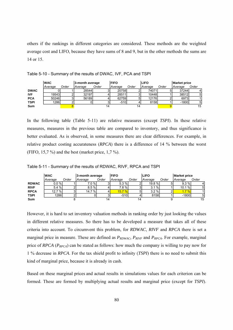
80
others if the rankings in different categories are considered. These methods are the weighted
average cost and LIFO, because they have sums of 8 and 9, but in the other methods the sums are
14 or 15.
Table 5-10 - Summary of the results of DWAC, IVF, PCA and TSPI
WAC 3-month average FIFO LIFO Market priceAverage Order Average Order Average Order Average Order Average Order
DWAC 0 1 28544 3 20758 2 74071 5 37244 4IVF 19543 2 32197 4 28511 3 10448 1 38512 5PCA 50246 3 56189 4 62759 5 12176 2 6973 1TSPI 1286 2 0 3 -510 4 8158 1 -1800 5Sum 8 14 14 9 15
In the following table (Table 5-11) are relative measures (except TSPI). In these relative
measures, measures in the previous table are compared to inventory, and thus significance is
better evaluated. As is observed, in some measures there are clear differences. For example, in
relative product costing accurateness (RPCA) there is a difference of 14 % between the worst
(FIFO, 15,7 %) and the best (market price, 1,7 %).
Table 5-11 - Summary of the results of RDWAC, RIVF, RPCA and TSPI
WAC 3-month average FIFO LIFO Market priceAverage Order Average Order Average Order Average Order Average Order
RDWAC 0.0 % 1 7.0 % 3 5.3 % 2 19.8 % 5 9.3 % 4RIVF 5.4 % 2 8.5 % 4 7.8 % 3 3.1 % 1 10.1 % 5RPCA 12.7 % 3 14.7 % 4 15.7 % 5 3.2 % 2 1.7 % 1TSPI 1286 2 0 3 -510 4 8158 1 -1800 5Sum 8 14 14 9 15
However, it is hard to set inventory valuation methods in ranking order by just looking the values
in different relative measures. So there has to be developed a measure that takes all of these
criteria into account. To circumvent this problem, for RDWAC, RIVF and RPCA there is set a
marginal price in measure. These are defined as PRDWAC, PRIVF and PRPCA. For example, marginal
price of RPCA (PRPCA) can be stated as follows: how much the company is willing to pay now for
1 % decrease in RPCA. For the tax shield profit to infinity (TSPI) there is no need to submit this
kind of marginal price, because it is already in cash.
Based on these marginal prices and actual results in simulations values for each criterion can be
formed. These are formed by multiplying actual results and marginal price (except for TSPI).
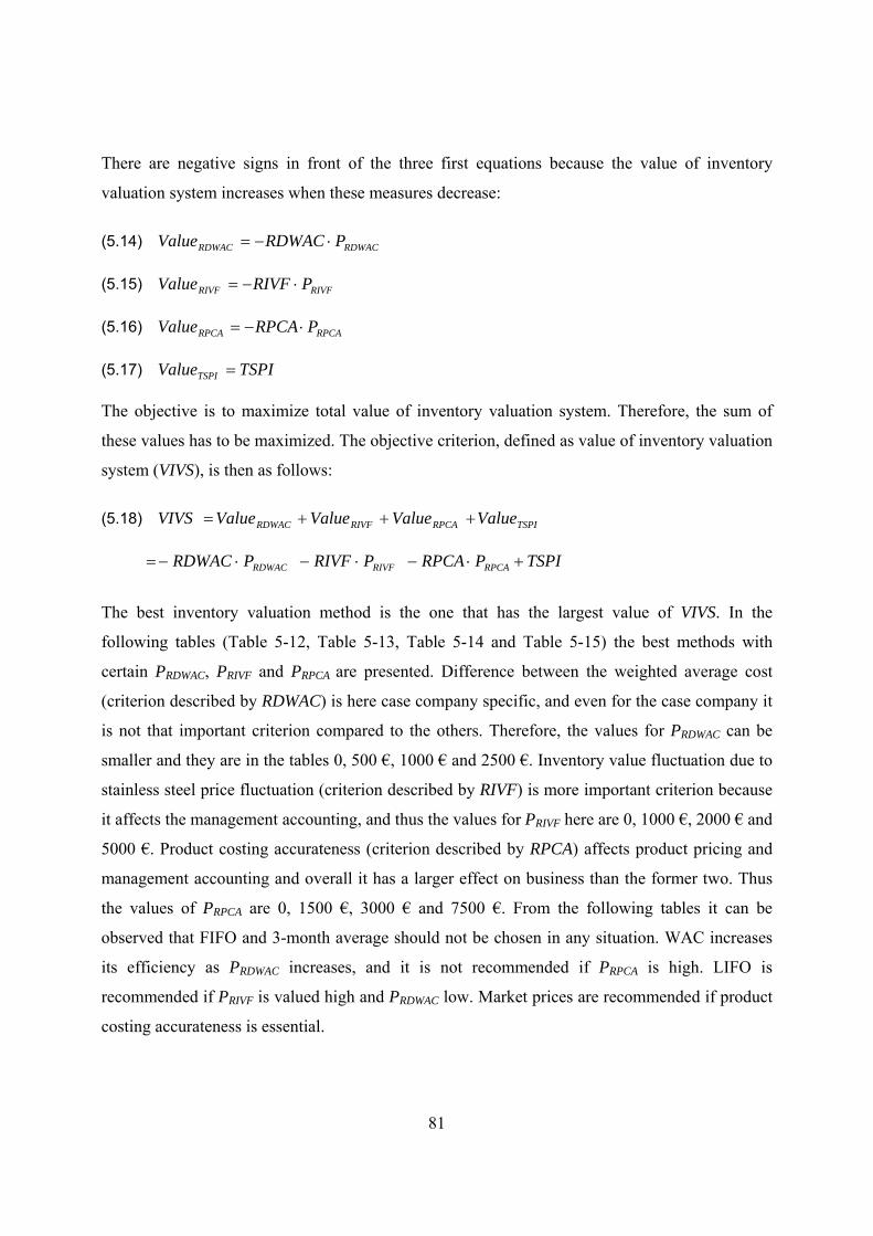
81
There are negative signs in front of the three first equations because the value of inventory
valuation system increases when these measures decrease:
(5.14) RDWACRDWAC PRDWACValue ⋅−=
(5.15) RIVFRIVF PRIVFValue ⋅−=
(5.16) RPCARPCA PRPCAValue ⋅−=
(5.17) TSPIValueTSPI =
The objective is to maximize total value of inventory valuation system. Therefore, the sum of
these values has to be maximized. The objective criterion, defined as value of inventory valuation
system (VIVS), is then as follows:
(5.18) TSPIRPCARIVFRDWAC ValueValueValueValueVIVS +++=
TSPIPRPCAPRIVFPRDWAC RPCARIVFRDWAC +⋅−⋅−⋅−=
The best inventory valuation method is the one that has the largest value of VIVS. In the
following tables (Table 5-12, Table 5-13, Table 5-14 and Table 5-15) the best methods with
certain PRDWAC, PRIVF and PRPCA are presented. Difference between the weighted average cost
(criterion described by RDWAC) is here case company specific, and even for the case company it
is not that important criterion compared to the others. Therefore, the values for PRDWAC can be
smaller and they are in the tables 0, 500 €, 1000 € and 2500 €. Inventory value fluctuation due to
stainless steel price fluctuation (criterion described by RIVF) is more important criterion because
it affects the management accounting, and thus the values for PRIVF here are 0, 1000 €, 2000 € and
5000 €. Product costing accurateness (criterion described by RPCA) affects product pricing and
management accounting and overall it has a larger effect on business than the former two. Thus
the values of PRPCA are 0, 1500 €, 3000 € and 7500 €. From the following tables it can be
observed that FIFO and 3-month average should not be chosen in any situation. WAC increases
its efficiency as PRDWAC increases, and it is not recommended if PRPCA is high. LIFO is
recommended if PRIVF is valued high and PRDWAC low. Market prices are recommended if product
costing accurateness is essential.
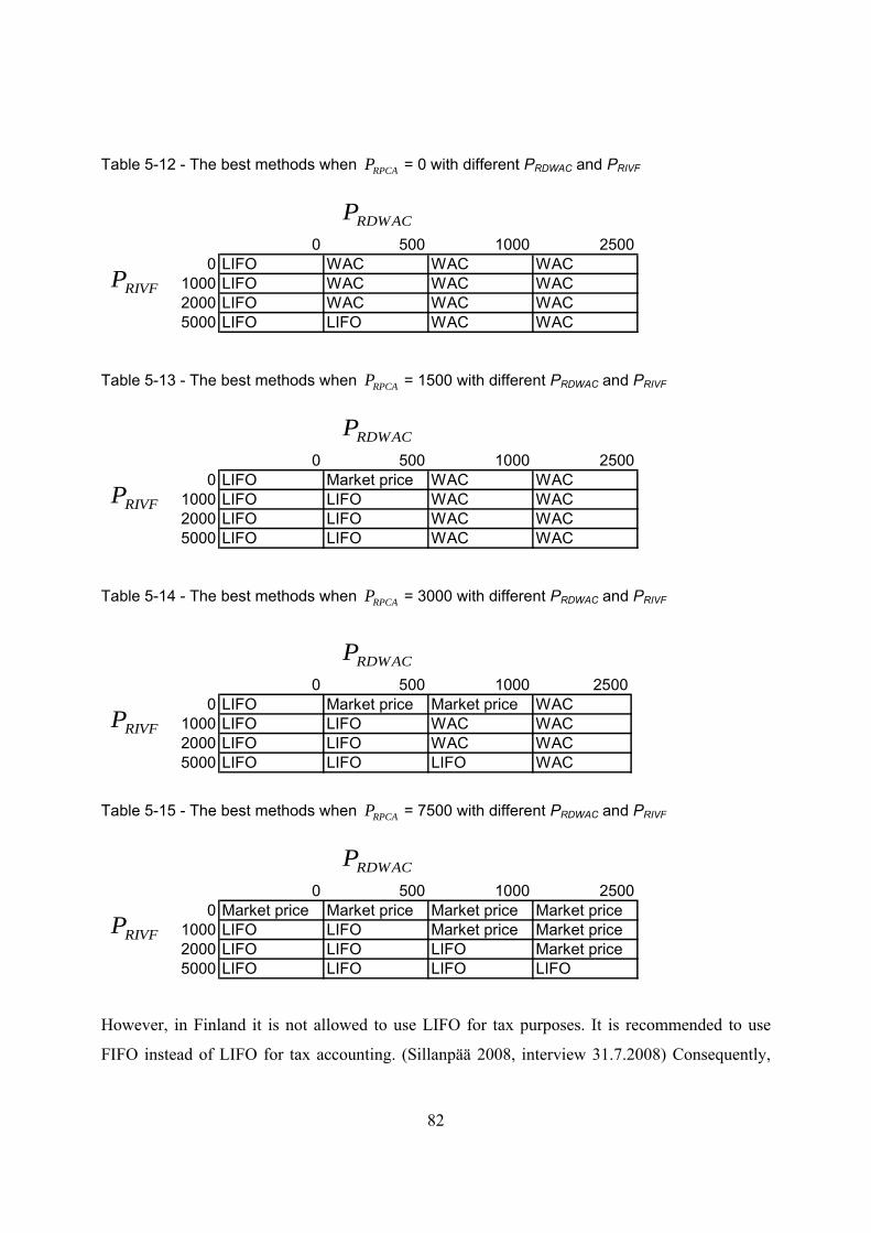
82
Table 5-12 - The best methods when RPCAP = 0 with different PRDWAC and PRIVF
0 500 1000 25000 LIFO WAC WAC WAC
1000 LIFO WAC WAC WAC2000 LIFO WAC WAC WAC5000 LIFO LIFO WAC WAC
RDWACP
RIVFP
Table 5-13 - The best methods when RPCAP = 1500 with different PRDWAC and PRIVF
0 500 1000 25000 LIFO Market price WAC WAC
1000 LIFO LIFO WAC WAC2000 LIFO LIFO WAC WAC5000 LIFO LIFO WAC WAC
RDWACP
RIVFP
Table 5-14 - The best methods when RPCAP = 3000 with different PRDWAC and PRIVF
0 500 1000 25000 LIFO Market price Market price WAC
1000 LIFO LIFO WAC WAC2000 LIFO LIFO WAC WAC5000 LIFO LIFO LIFO WAC
RDWACP
RIVFP
Table 5-15 - The best methods when RPCAP = 7500 with different PRDWAC and PRIVF
0 500 1000 25000 Market price Market price Market price Market price
1000 LIFO LIFO Market price Market price2000 LIFO LIFO LIFO Market price5000 LIFO LIFO LIFO LIFO
RDWACP
RIVFP
However, in Finland it is not allowed to use LIFO for tax purposes. It is recommended to use
FIFO instead of LIFO for tax accounting. (Sillanpää 2008, interview 31.7.2008) Consequently,
83
VIVS needs to be modified in the case of LIFO. It is done by letting TSPI of LIFO to be as much
as TSPI of FIFO. In the next tables the best methods under this assumption are presented.
Table 5-16 - The best methods in Finland when RPCAP = 0 with different PRDWAC and PRIVF
0 500 1000 25000 WAC WAC WAC WAC
1000 LIFO WAC WAC WAC2000 LIFO WAC WAC WAC5000 LIFO LIFO WAC WAC
RDWACP
RIVFP
Table 5-17 - The best methods in Finland when RPCAP = 1500 with different PRDWAC and PRIVF
0 500 1000 25000 Market price Market price WAC WAC
1000 LIFO WAC WAC WAC2000 LIFO LIFO WAC WAC5000 LIFO LIFO WAC WAC
RDWACP
RIVFP
Table 5-18 - The best methods in Finland when RPCAP = 3000 with different PRDWAC and PRIVF
0 500 1000 25000 Market price Market price Market price WAC
1000 LIFO LIFO WAC WAC2000 LIFO LIFO WAC WAC5000 LIFO LIFO LIFO WAC
RDWACP
RIVFP
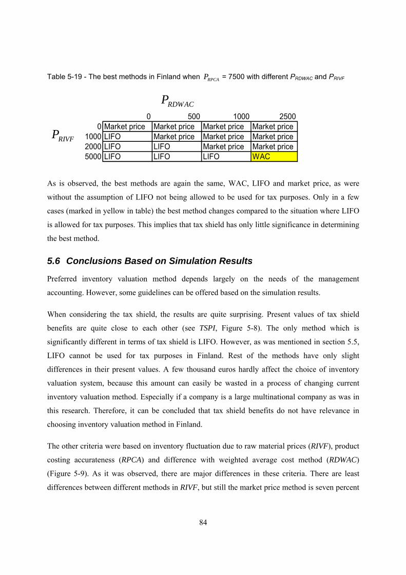
84
Table 5-19 - The best methods in Finland when RPCAP = 7500 with different PRDWAC and PRIVF
0 500 1000 25000 Market price Market price Market price Market price
1000 LIFO Market price Market price Market price2000 LIFO LIFO Market price Market price5000 LIFO LIFO LIFO WAC
RDWACP
RIVFP
As is observed, the best methods are again the same, WAC, LIFO and market price, as were
without the assumption of LIFO not being allowed to be used for tax purposes. Only in a few
cases (marked in yellow in table) the best method changes compared to the situation where LIFO
is allowed for tax purposes. This implies that tax shield has only little significance in determining
the best method.
5.6 Conclusions Based on Simulation Results
Preferred inventory valuation method depends largely on the needs of the management
accounting. However, some guidelines can be offered based on the simulation results.
When considering the tax shield, the results are quite surprising. Present values of tax shield
benefits are quite close to each other (see TSPI, Figure 5-8). The only method which is
significantly different in terms of tax shield is LIFO. However, as was mentioned in section 5.5,
LIFO cannot be used for tax purposes in Finland. Rest of the methods have only slight
differences in their present values. A few thousand euros hardly affect the choice of inventory
valuation system, because this amount can easily be wasted in a process of changing current
inventory valuation method. Especially if a company is a large multinational company as was in
this research. Therefore, it can be concluded that tax shield benefits do not have relevance in
choosing inventory valuation method in Finland.
The other criteria were based on inventory fluctuation due to raw material prices (RIVF), product
costing accurateness (RPCA) and difference with weighted average cost method (RDWAC)
(Figure 5-9). As it was observed, there are major differences in these criteria. There are least
differences between different methods in RIVF, but still the market price method is seven percent
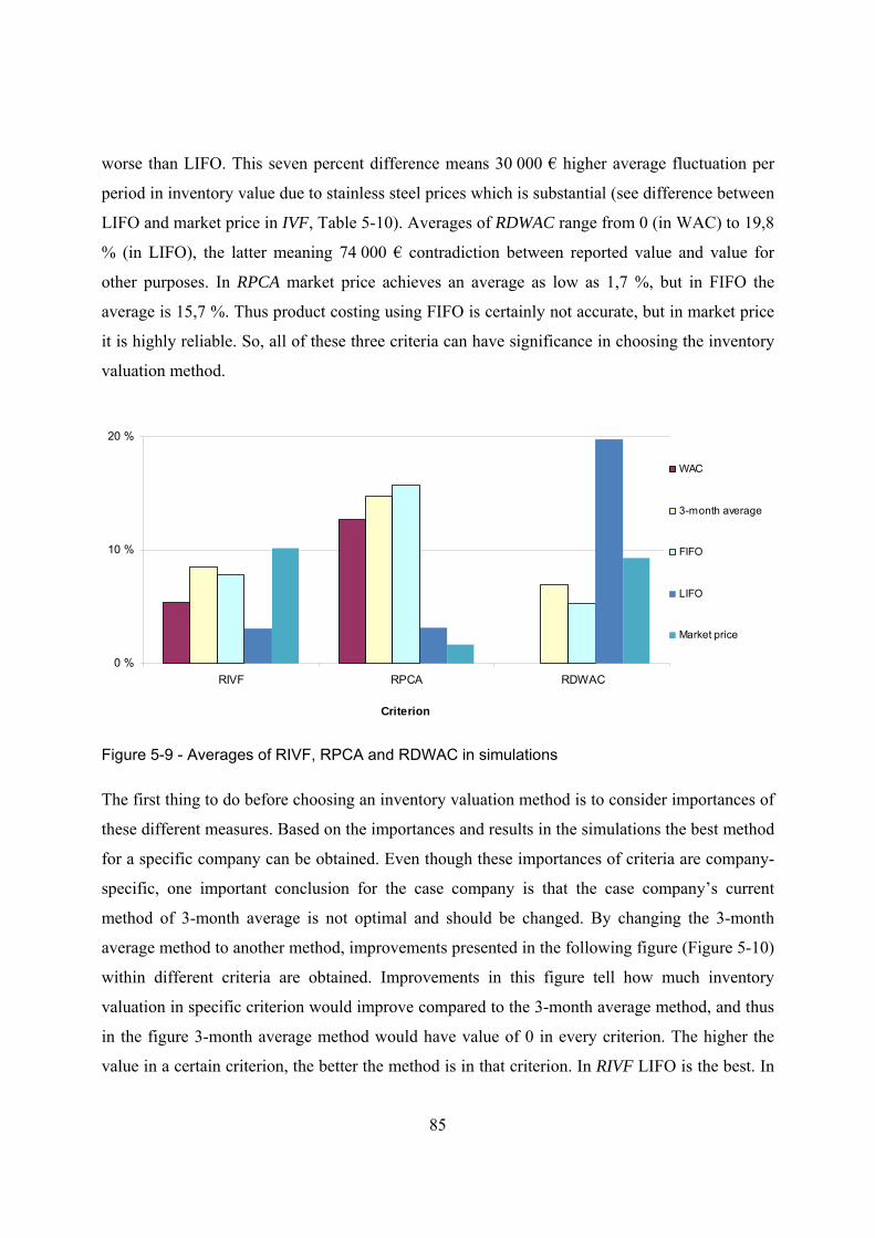
85
worse than LIFO. This seven percent difference means 30 000 € higher average fluctuation per
period in inventory value due to stainless steel prices which is substantial (see difference between
LIFO and market price in IVF, Table 5-10). Averages of RDWAC range from 0 (in WAC) to 19,8
% (in LIFO), the latter meaning 74 000 € contradiction between reported value and value for
other purposes. In RPCA market price achieves an average as low as 1,7 %, but in FIFO the
average is 15,7 %. Thus product costing using FIFO is certainly not accurate, but in market price
it is highly reliable. So, all of these three criteria can have significance in choosing the inventory
valuation method.
0 %
10 %
20 %
RIVF RPCA RDWAC
Criterion
WAC
3-month average
FIFO
LIFO
Market price
Figure 5-9 - Averages of RIVF, RPCA and RDWAC in simulations
The first thing to do before choosing an inventory valuation method is to consider importances of
these different measures. Based on the importances and results in the simulations the best method
for a specific company can be obtained. Even though these importances of criteria are company-
specific, one important conclusion for the case company is that the case company’s current
method of 3-month average is not optimal and should be changed. By changing the 3-month
average method to another method, improvements presented in the following figure (Figure 5-10)
within different criteria are obtained. Improvements in this figure tell how much inventory
valuation in specific criterion would improve compared to the 3-month average method, and thus
in the figure 3-month average method would have value of 0 in every criterion. The higher the
value in a certain criterion, the better the method is in that criterion. In RIVF LIFO is the best. In
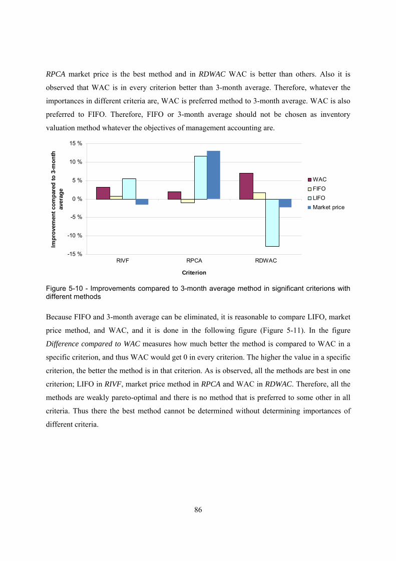
86
RPCA market price is the best method and in RDWAC WAC is better than others. Also it is
observed that WAC is in every criterion better than 3-month average. Therefore, whatever the
importances in different criteria are, WAC is preferred method to 3-month average. WAC is also
preferred to FIFO. Therefore, FIFO or 3-month average should not be chosen as inventory
valuation method whatever the objectives of management accounting are.
-15 %
-10 %
-5 %
0 %
5 %
10 %
15 %
RIVF RPCA RDWAC
Criterion
Impr
ovem
ent c
ompa
red
to 3
-mon
th
aver
age
WAC FIFOLIFOMarket price
Figure 5-10 - Improvements compared to 3-month average method in significant criterions with different methods
Because FIFO and 3-month average can be eliminated, it is reasonable to compare LIFO, market
price method, and WAC, and it is done in the following figure (Figure 5-11). In the figure
Difference compared to WAC measures how much better the method is compared to WAC in a
specific criterion, and thus WAC would get 0 in every criterion. The higher the value in a specific
criterion, the better the method is in that criterion. As is observed, all the methods are best in one
criterion; LIFO in RIVF, market price method in RPCA and WAC in RDWAC. Therefore, all the
methods are weakly pareto-optimal and there is no method that is preferred to some other in all
criteria. Thus there the best method cannot be determined without determining importances of
different criteria.
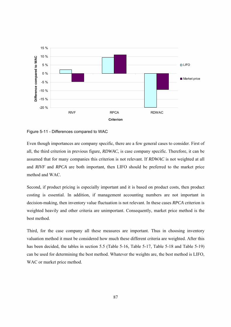
87
-20 %
-15 %
-10 %
-5 %
0 %
5 %
10 %
15 %
RIVF RPCA RDWAC
Criterion
Diffe
renc
e co
mpa
red
to W
AC
LIFO
Market price
Figure 5-11 - Differences compared to WAC
Even though importances are company specific, there are a few general cases to consider. First of
all, the third criterion in previous figure, RDWAC, is case company specific. Therefore, it can be
assumed that for many companies this criterion is not relevant. If RDWAC is not weighted at all
and RIVF and RPCA are both important, then LIFO should be preferred to the market price
method and WAC.
Second, if product pricing is especially important and it is based on product costs, then product
costing is essential. In addition, if management accounting numbers are not important in
decision-making, then inventory value fluctuation is not relevant. In these cases RPCA criterion is
weighted heavily and other criteria are unimportant. Consequently, market price method is the
best method.
Third, for the case company all these measures are important. Thus in choosing inventory
valuation method it must be considered how much these different criteria are weighted. After this
has been decided, the tables in section 5.5 (Table 5-16, Table 5-17, Table 5-18 and Table 5-19)
can be used for determining the best method. Whatever the weights are, the best method is LIFO,
WAC or market price method.
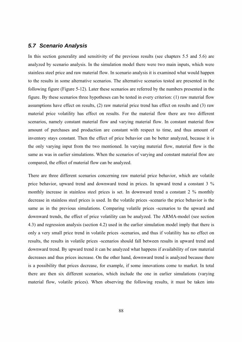
88
5.7 Scenario Analysis
In this section generality and sensitivity of the previous results (see chapters 5.5 and 5.6) are
analyzed by scenario analysis. In the simulation model there were two main inputs, which were
stainless steel price and raw material flow. In scenario analysis it is examined what would happen
to the results in some alternative scenarios. The alternative scenarios tested are presented in the
following figure (Figure 5-12). Later these scenarios are referred by the numbers presented in the
figure. By these scenarios three hypotheses can be tested in every criterion: (1) raw material flow
assumptions have effect on results, (2) raw material price trend has effect on results and (3) raw
material price volatility has effect on results. For the material flow there are two different
scenarios, namely constant material flow and varying material flow. In constant material flow
amount of purchases and production are constant with respect to time, and thus amount of
inventory stays constant. Then the effect of price behavior can be better analyzed, because it is
the only varying input from the two mentioned. In varying material flow, material flow is the
same as was in earlier simulations. When the scenarios of varying and constant material flow are
compared, the effect of material flow can be analyzed.
There are three different scenarios concerning raw material price behavior, which are volatile
price behavior, upward trend and downward trend in prices. In upward trend a constant 3 %
monthly increase in stainless steel prices is set. In downward trend a constant 2 % monthly
decrease in stainless steel prices is used. In the volatile prices -scenario the price behavior is the
same as in the previous simulations. Comparing volatile prices -scenarios to the upward and
downward trends, the effect of price volatility can be analyzed. The ARMA-model (see section
4.3) and regression analysis (section 4.2) used in the earlier simulation model imply that there is
only a very small price trend in volatile prices -scenarios, and thus if volatility has no effect on
results, the results in volatile prices -scenarios should fall between results in upward trend and
downward trend. By upward trend it can be analyzed what happens if availability of raw material
decreases and thus prices increase. On the other hand, downward trend is analyzed because there
is a possibility that prices decrease, for example, if some innovations come to market. In total
there are then six different scenarios, which include the one in earlier simulations (varying
material flow, volatile prices). When observing the following results, it must be taken into
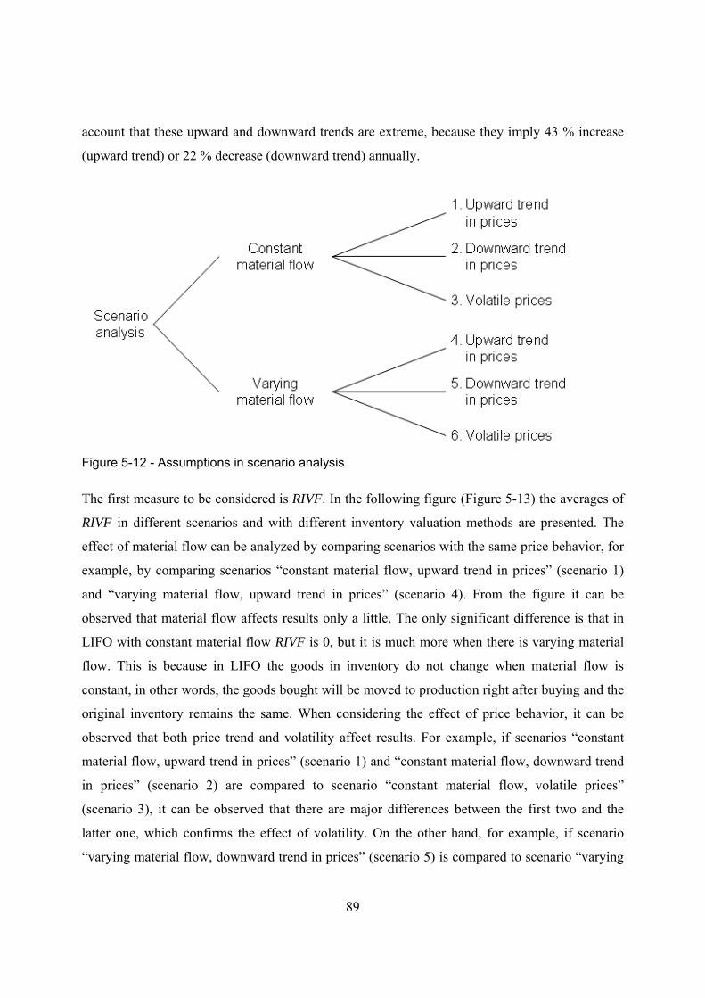
89
account that these upward and downward trends are extreme, because they imply 43 % increase
(upward trend) or 22 % decrease (downward trend) annually.
Figure 5-12 - Assumptions in scenario analysis
The first measure to be considered is RIVF. In the following figure (Figure 5-13) the averages of
RIVF in different scenarios and with different inventory valuation methods are presented. The
effect of material flow can be analyzed by comparing scenarios with the same price behavior, for
example, by comparing scenarios “constant material flow, upward trend in prices” (scenario 1)
and “varying material flow, upward trend in prices” (scenario 4). From the figure it can be
observed that material flow affects results only a little. The only significant difference is that in
LIFO with constant material flow RIVF is 0, but it is much more when there is varying material
flow. This is because in LIFO the goods in inventory do not change when material flow is
constant, in other words, the goods bought will be moved to production right after buying and the
original inventory remains the same. When considering the effect of price behavior, it can be
observed that both price trend and volatility affect results. For example, if scenarios “constant
material flow, upward trend in prices” (scenario 1) and “constant material flow, downward trend
in prices” (scenario 2) are compared to scenario “constant material flow, volatile prices”
(scenario 3), it can be observed that there are major differences between the first two and the
latter one, which confirms the effect of volatility. On the other hand, for example, if scenario
“varying material flow, downward trend in prices” (scenario 5) is compared to scenario “varying
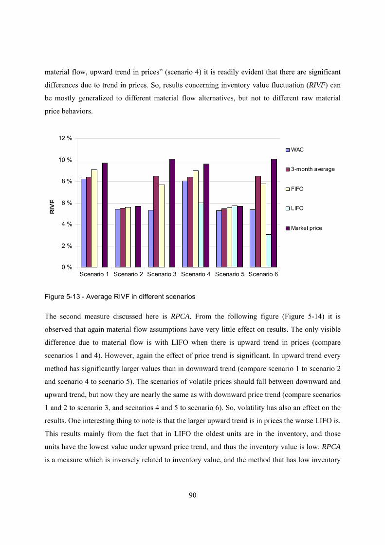
90
material flow, upward trend in prices” (scenario 4) it is readily evident that there are significant
differences due to trend in prices. So, results concerning inventory value fluctuation (RIVF) can
be mostly generalized to different material flow alternatives, but not to different raw material
price behaviors.
0 %
2 %
4 %
6 %
8 %
10 %
12 %
Scenario 1 Scenario 2 Scenario 3 Scenario 4 Scenario 5 Scenario 6
RIV
F
WAC
3-month average
FIFO
LIFO
Market price
Figure 5-13 - Average RIVF in different scenarios
The second measure discussed here is RPCA. From the following figure (Figure 5-14) it is
observed that again material flow assumptions have very little effect on results. The only visible
difference due to material flow is with LIFO when there is upward trend in prices (compare
scenarios 1 and 4). However, again the effect of price trend is significant. In upward trend every
method has significantly larger values than in downward trend (compare scenario 1 to scenario 2
and scenario 4 to scenario 5). The scenarios of volatile prices should fall between downward and
upward trend, but now they are nearly the same as with downward price trend (compare scenarios
1 and 2 to scenario 3, and scenarios 4 and 5 to scenario 6). So, volatility has also an effect on the
results. One interesting thing to note is that the larger upward trend is in prices the worse LIFO is.
This results mainly from the fact that in LIFO the oldest units are in the inventory, and those
units have the lowest value under upward price trend, and thus the inventory value is low. RPCA
is a measure which is inversely related to inventory value, and the method that has low inventory
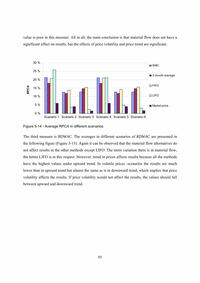
91
value is poor in this measure. All in all, the main conclusion is that material flow does not have a
significant effect on results, but the effects of price volatility and price trend are significant.
0 %
5 %
10 %
15 %
20 %
25 %
30 %
Scenario 1 Scenario 2 Scenario 3 Scenario 4 Scenario 5 Scenario 6
RPCA
WAC
3-month average
FIFO
LIFO
Market price
Figure 5-14 - Average RPCA in different scenarios
The third measure is RDWAC. The averages in different scenarios of RDWAC are presented in
the following figure (Figure 5-15). Again it can be observed that the material flow alternatives do
not affect results in the other methods except LIFO. The more variation there is in material flow,
the better LIFO is in this respect. However, trend in prices affects results because all the methods
have the highest values under upward trend. In volatile prices -scenarios the results are much
lower than in upward trend but almost the same as is in downward trend, which implies that price
volatility affects the results. If price volatility would not affect the results, the values should fall
between upward and downward trend.
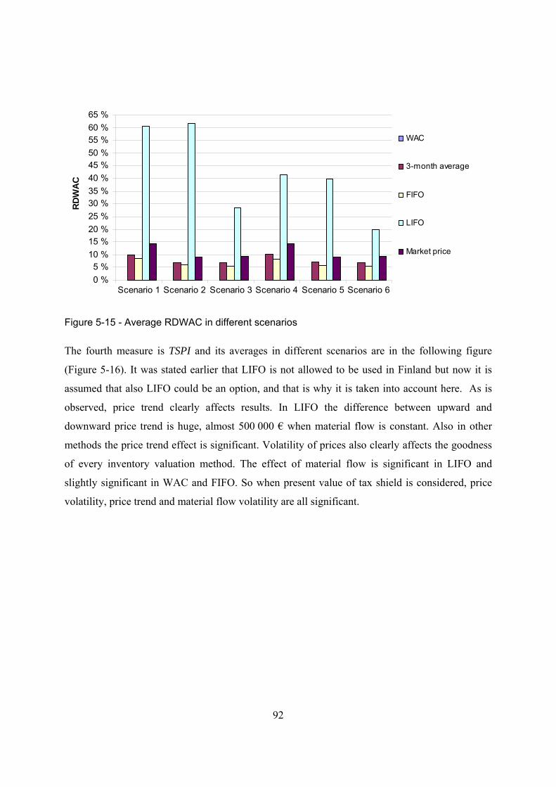
92
0 %5 %
10 %15 %20 %25 %30 %35 %40 %45 %50 %55 %60 %65 %
Scenario 1 Scenario 2 Scenario 3 Scenario 4 Scenario 5 Scenario 6
RDW
AC
WAC
3-month average
FIFO
LIFO
Market price
Figure 5-15 - Average RDWAC in different scenarios
The fourth measure is TSPI and its averages in different scenarios are in the following figure
(Figure 5-16). It was stated earlier that LIFO is not allowed to be used in Finland but now it is
assumed that also LIFO could be an option, and that is why it is taken into account here. As is
observed, price trend clearly affects results. In LIFO the difference between upward and
downward price trend is huge, almost 500 000 € when material flow is constant. Also in other
methods the price trend effect is significant. Volatility of prices also clearly affects the goodness
of every inventory valuation method. The effect of material flow is significant in LIFO and
slightly significant in WAC and FIFO. So when present value of tax shield is considered, price
volatility, price trend and material flow volatility are all significant.
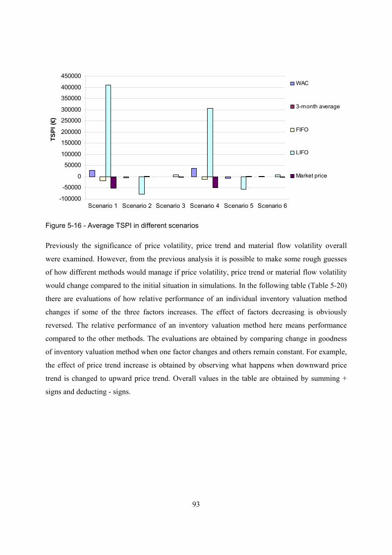
93
-100000
-50000
0
50000
100000
150000
200000
250000
300000
350000
400000
450000
Scenario 1 Scenario 2 Scenario 3 Scenario 4 Scenario 5 Scenario 6
TSPI
(€)
WAC
3-month average
FIFO
LIFO
Market price
Figure 5-16 - Average TSPI in different scenarios
Previously the significance of price volatility, price trend and material flow volatility overall
were examined. However, from the previous analysis it is possible to make some rough guesses
of how different methods would manage if price volatility, price trend or material flow volatility
would change compared to the initial situation in simulations. In the following table (Table 5-20)
there are evaluations of how relative performance of an individual inventory valuation method
changes if some of the three factors increases. The effect of factors decreasing is obviously
reversed. The relative performance of an inventory valuation method here means performance
compared to the other methods. The evaluations are obtained by comparing change in goodness
of inventory valuation method when one factor changes and others remain constant. For example,
the effect of price trend increase is obtained by observing what happens when downward price
trend is changed to upward price trend. Overall values in the table are obtained by summing +
signs and deducting - signs.
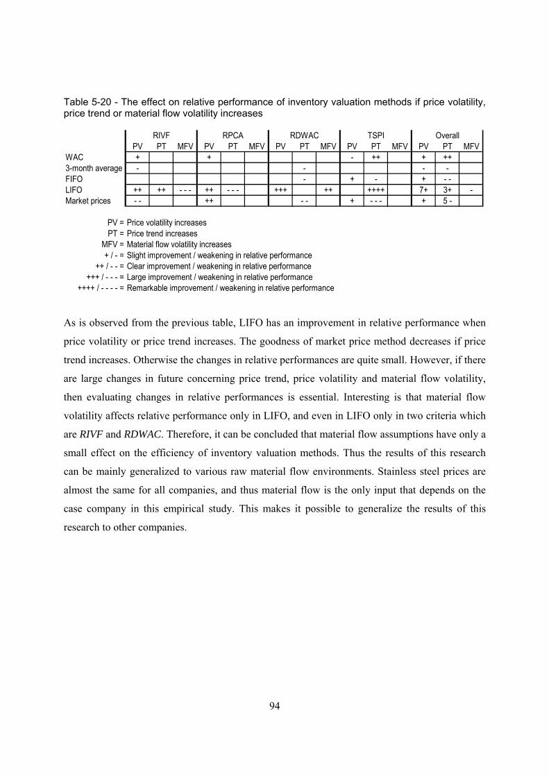
94
Table 5-20 - The effect on relative performance of inventory valuation methods if price volatility, price trend or material flow volatility increases
RIVF RPCA RDWAC TSPI OverallPV PT MFV PV PT MFV PV PT MFV PV PT MFV PV PT MFV
WAC + + - ++ + ++3-month average - - - -FIFO - + - + - -LIFO ++ ++ - - - ++ - - - +++ ++ ++++ 7+ 3+ -Market prices - - ++ - - + - - - + 5 -
PV = Price volatility increasesPT = Price trend increases
MFV = Material flow volatility increases+ / - = Slight improvement / weakening in relative performance
++ / - - = Clear improvement / weakening in relative performance+++ / - - - = Large improvement / weakening in relative performance
++++ / - - - - = Remarkable improvement / weakening in relative performance
As is observed from the previous table, LIFO has an improvement in relative performance when
price volatility or price trend increases. The goodness of market price method decreases if price
trend increases. Otherwise the changes in relative performances are quite small. However, if there
are large changes in future concerning price trend, price volatility and material flow volatility,
then evaluating changes in relative performances is essential. Interesting is that material flow
volatility affects relative performance only in LIFO, and even in LIFO only in two criteria which
are RIVF and RDWAC. Therefore, it can be concluded that material flow assumptions have only a
small effect on the efficiency of inventory valuation methods. Thus the results of this research
can be mainly generalized to various raw material flow environments. Stainless steel prices are
almost the same for all companies, and thus material flow is the only input that depends on the
case company in this empirical study. This makes it possible to generalize the results of this
research to other companies.
95
6 Conclusions In the literature review it was observed that product costing and inventory valuation are left
uncovered from the viewpoint of fluctuating raw material prices, even though these two topics
are largely covered even from mid 20th century from a number of viewpoints. Uncertainty of raw
material prices affects every objective of management accounting, which are supplying
information for internal decision makers, facilitating their decision making, motivating their
actions and behavior in a given direction and promoting efficiency of the organization. All
previous objectives are heavily affected by this uncertainty, and thus it has a large impact on
business performance. Another gap in the current research is that overall situation of a company
in choosing inventory valuation and product costing policies has not been analyzed thoroughly.
Most of the researches focus on just one or a few factors that affect the choice of inventory
valuation policies.
Due to these gaps in the current research, this research focused on analyzing efficient inventory
valuation and product costing policies under fluctuating raw material prices. To analyze these
methods as broadly as possible, a case company was chosen for this research. This research
included a literature review and an empirical study. The research method in the empirical study
was simulation, which was observed to be the best method for analyzing the effects of random
movements in raw material prices in the future. Various scenarios can be tested by simulation,
and based on these scenarios the best methods can be determined through versatile measures.
A brief summary of research progress is presented next, where the main parts of this research are
discussed. After the summary, integral results of this research are covered. In final part topics for
further research are discussed.
6.1 Summary
First an extensive literature review was carried out in order to analyze inventory valuation and
product costing in depth. The focus was on how a company should choose inventory valuation
and product costing policies. Due to raw materials being an important part of this research, also
the modeling of raw material prices was covered.
96
Despite the fact that inventory valuation and product costing have been researched for so long,
there is no consensus of the best methods. Researchers have been debating especially which one
of the following two is better: last-in first-out (LIFO) or first-in first-out (FIFO). Some
researchers argue that FIFO is the best method, for example, when there is a possibility of
manipulating accounting figures or a company has a high debt ratio. On the other hand, LIFO is
recommended when tax shield benefits can be significant or when pricing is based on product
costs. In order to create an overall view of all the valuation methods, large amount of research
papers were covered to form a list of factors that should affect the choice of inventory valuation
method. This list should be considered as a general guideline when choosing inventory valuation
method.
To take fluctuating raw material prices into consideration, an empirical study including the effect
of fluctuating raw material prices was made. Thus literature review included practices and
principles of modeling and forecasting raw material price movements. There are various models
that predict random movements in raw material prices. Maybe the best-known models are
moving-average and exponential smoothing. According to literature, an efficient method is
autoregressive moving-average (ARMA), which takes previous values (autoregressive part) and
previous errors (moving-average part) into account. For estimating volatility autoregressive
conditionally heteroskedasticity (ARCH) and generalized autoregressive conditionally
heteroskedasticity (GARCH) models are recommended. The best methods of forecasting actual
values and volatility still depend on the situation. For example, lack of data can be a problem
when forming complicated models.
Based on the literature review, a research framework for the empirical study was constructed.
The framework included three main variables that should affect the choice of raw material
inventory valuation and product costing policy: (1) how well information reflects company’s
performance, (2) effect on tax obligations and (3) product costing accurateness. Based on the
framework, evaluation criteria to evaluate different inventory valuation methods were
constructed. These criteria included present value of tax shield, inventory value fluctuation due to
stainless steel price, product costing accurateness and difference in inventory value compared to
inventory value of weighted average cost. The first three criteria were derived directly from the
97
variables in the research framework. The fourth criterion was based on the situation in the case
company.
To evaluate different inventory valuation methods based on the formed criteria, a simulation
model was built taking the overall situation of the case company into account. The main variable
in the simulation model was stainless steel price, which depends on nickel price. Thus nickel
price behavior was modeled. In addition, purchasing and production behavior were modeled for
the simulation model. Five different inventory valuation methods were tested which were FIFO,
LIFO, weighted average cost (WAC), market price and 3-month average. The first four were
found to be suitable for raw material accounting based on the literature and the last one was used
in the case company.
After simulations the results based on the evaluation criteria were formed in order to evaluate the
different methods. Since there were in total four criteria, and different companies appreciate these
criteria differently, a comprehensive sensitivity analysis considering various appreciations of
these criteria was done. Also, in order to analyze inventory valuation methods in different
situations a scenario analysis was done.
6.2 Integral Results
The research problem of this study was stated as follows: How should raw material flow around
raw material inventory be valuated? The main results of this research are presented in this
chapter. These results are based partly on the literature review but mainly on the empirical study.
The results are conducted with respect to the research objectives stated in the introduction
chapter.
The first research objective was to model stainless steel price behavior. To this end, it was
investigated whether stainless steel prices depend on any other variables. Based on regression
analysis, stainless steel prices depend primarily on nickel prices one, two and three months ago.
Therefore, nickel prices were modeled. In the literature review it was observed that
autoregressive moving-average forecasting method is a versatile method to model raw material
price movements. In the analysis it was found that future nickel prices depend only on the
previous nickel prices when monthly values are modeled. So autoregressive process of lag one
(AR(1)) was chosen for further analysis. Also volatility of nickel prices was analyzed and it was
98
found that volatility doesn’t depend on the previous volatilities. Consequently, constant variance
was chosen to model variance of nickel prices.
The second research objective was to find out factors that determine the best raw material
inventory valuation and product costing policy. It was observed that there are eight main factors
that should be taken into account when choosing inventory valuation policy, and they are (1)
complexity of IT-systems, (2) how much pricing is based on product costs, (3) how probable is
manipulation of accounting measures, (4) restrictive debt covenants, (5) debt ratio, (6) potential
tax savings, (7) firm size and (8) volatility of earnings. By these factors inventory valuation
methods overall can be evaluated. However, this research was about valuating raw material
inventory, and thus based on these factors raw material inventory valuation method cannot be
straightforwardly determined.
The third research objective was to find out the most efficient way to value raw material
inventory. In the literature review it was observed that this objective is highly related to the fourth
research objective, which was to discover the most efficient way to value raw material flow out
of inventory. The reason for this is that the same method has to be used for both raw material
inventory valuation and product costing purposes. Thus these two objectives were analyzed
together. In the simulation model five different raw material inventory valuation methods were
analyzed by evaluation criteria. Overall, last-in first-out (LIFO), weighted average cost (WAC)
and market price method turned out to be very promising. LIFO was best in two criteria, which
imply that tax shield benefits are high and inventory value is nonvolatile in LIFO. Weighted
average cost was in top three in every criterion, and thus it was the most consistent in this sense.
Market price method is especially good for product costing. Surprisingly, FIFO and current
method in the case company (3-month average) should not be used for raw material accounting in
any situation. Changing the current method would yield high improvements. For example,
changing to LIFO would decrease product costing error from 14,7 to 3,2 percent of product costs
and inventory value fluctuation due to stainless steel price from 8,5 to 3,1 percent of inventory
value. The choice between LIFO, market price and WAC depend on the objectives of inventory
valuation because all these measures are weakly pareto-optimal.
The results of this research contribute well to the previous research around inventory valuation
and product costing. As mentioned, inventory valuation and product costing, when raw materials
99
are considered, are not even nearly completely covered, although there does exist research around
these topics from mid 20th century. Especially there does not exist a research that covers these
two topics under volatile raw material, and thus this research fills a major gap in current research.
From the viewpoint of companies that struggle with volatile raw material prices this research can
be an important asset when considering how to improve raw material inventory valuation and
product costing. Also, the simulation model of this research can easily be extended to other raw
materials. For example, oil prices have been volatile in recent years and extending this simulation
model for oil could be worthwhile.
6.3 Further Research
The objective of this research was to investigate how to value raw material flow around raw
material inventory. This research succeeded well in meeting its objectives defined in the
introduction of this research (see chapter 1.2). However, in the area of this research a lot more
further research is needed. Especially the following two topics need to be researched further.
The raw material in this research was stainless steel. Stainless steel prices are dependent on
nickel prices, and the relation was modeled with regression analysis. The regression analysis
itself limits generality only a little. Some additional error still exists due to the fact that the
parameters of the model are let to vary in some extent in the simulation model. However,
primarily the results of this research can be generalized to raw materials that have similar price
behavior as nickel has. Nickel prices behave as AR(1)-model. In the scenario analysis (see
chapter 5.7) it was observed that the results of this research cannot be generalized to other kinds
of price behaviors. Therefore, one topic for further research would be conducting this research for
raw materials that have price behavior different than AR(1)-model.
This research focused on raw materials and therefore semi-finished and end-products were set to
be beyond the scope of this research. The methods here were chosen to be consistent with raw
materials, and thus these results cannot be generalized to semi-finished or end-products. End-
products often form the largest share of inventory value. Thus it would be interesting to
investigate how these results differ if end-products are the focus of research.
100
References
Articles and Books
Ali Group (2007) Consolidation manual, FY 2007, Ali Group, Italy.
Alnestig, P. & Segerstedt, A. (1996) “Product costing in ten Swedish manufacturing companies”, International Journal of Production Economics, Vol. 46–47, No. 1, pp. 441–457.
Amaratunga, D., Baldry, D., Sarshar, M. & Newton, R. (2002) “Quantitative and qualitative research in the built environment: application of “mixed” research approach”, Work Study, Vol. 51, No.1, pp. 17–31.
Astami, E. W. & Tower, G. (2006) “Accounting-policy choice and firm characteristics in Asia Pacific region: An international empirical test of Costly Contracting Theory”, The International Journal of Accounting, Vol. 41, No. 1, pp. 1–21.
Banks, J. & Gibson, R. (1997) “Don’t Simulate When… 10 Rules for Determining when Simulation is Not Appropriate”, IIE Solutions, Vol. 29, No. 9, pp. 30–32.
Banks, J., Carson, J. S. II, Nelson, B. L. & Nicol, D. M. (2005) Discrete-Event System Simulation, 4th Edition, Pearson Prentice Hall, Upper Saddle River, US, 624 p.
Bar-Yosef, S. & Sen, P. K. (1992) “On Optimal Choice of Inventory Accounting Method”, Accounting Review, Vol. 67, No. 2, pp. 320–336.
Belkaoui, A. (1980) Conceptual Foundations of Management Accounting, Addison-Wesley, Reading, US, 120 p.
Bera, A. K. & Higgins, M. L. (1993) “ARCH Models: Properties, Estimation and Testing,” Journal of Economic Surveys, Vol. 7, No. 4, pp. 307–366.
Berry, W. D. & Feldman, S. F. (1985) Multiple Regression in Practice, Series of Quantitative Applications in the Social Sciences, Sage University Papers, London, United Kingdom, 96 p. Biddle, G. C. (1980) “Accounting Methods and Management Decisions: The Case of Inventory Costing and Inventory Policy”, Journal of Accounting Research, Vol. 18, pp. 235–280.
Bierman, H. Jr. (1959) “Pricing Intracompany Transfers”, The Accounting Review, Vol. 34, No. 3, pp. 429–432.
Bierman, H. Jr. (1967) “Inventory Valuation: The Use of Market Prices”, The Accounting Review, Vol. 42, No. 4, pp. 731–737.
101
Bragg, S. M. (2005) Inventory Accounting: A Comprehensive Guide, John Wiley & Sons Inc, Hoboken, US, 243 p.
Brooks, C. (2002) Introductory econometrics for finance, Cambridge University Press, Cambridge, United Kingdom, 701 p.
Bryman, A. & Bell, E. (2003) Business Research Methods, Oxford University Press, Oxford, United Kingdom, 624 p.
Campbell, R. J. (1995) “Steeling time with ABC or TOC”. Management Accounting, Vol. 76, No. 7, pp. 31.
Campbell, R., Brewer, P. & Mills, T. (1997) “Designing an Information System Using Activity-Based Costing and the Theory of Constraints”, Journal of Cost Management, Vol. 11, No. 1, pp. 16-25.
Chadwick, L. (2002) Essential Finance and Accounting for Managers, Pearson Education Limited, Essex, United Kingdom, 435 p.
Cooper, R. & Kaplan, R. S. (1991) “Profit Priorities from Activity-Based Costing”, Harvard Business Review, Vol. 69, No. 3, pp. 130–135.
Cushing, B. E. & LeClere, M. J. (1992) “Evidence on the Determinants of Inventory Accounting Policy Choice”, The Accounting Review, Vol. 67, No. 2, pp. 355–366.
Datar, S. & Gupta, M. (1994) “Aggregation, Specification and Measurement Errors in Product Costing”, The Accounting Review, Vol. 69, No. 4, pp. 567–591.
Dean, J. (1955) “Decentralization and Intracompany Pricing”, Harvard Business Review, Vol. 33, No. 4, pp. 65–74.
Dhaliwal, D. S. (1980) “The Effect of the Firm's Capital Structure on the Choice of Accounting Methods", The Accounting Review, Vol. 55, No. 1, pp. 78–84.
Dominiak, G. F. & Louderback, J. G. (1994) Managerial Accounting, 7th Edition, South-Western Publishing Co., Cincinnati, US, 846 p.
Dooley, K. (2002) “Simulation Research Methods”, in Baum J. (eds.) Companion to Organizations, Blackwell, London, United Kingdom, pp. 829–848.
Dopuch, N. & Pincus, M. (1988) “Evidence on the Choice of Inventory Accounting Methods: LIFO Versus FIFO”, Journal of Accounting Research, Vol. 26, No. 1, pp. 28–59.
Dougherty, C. (2002) Introduction to Econometrics, Oxford University Press, New York, US, 424 p.
Fanning, D. (1983) Handbook of Management Accounting, Gower Publishing Company Limited, Aldershot, United Kingdom, 471 p.
102
Farnum, N. R. & Stanton, L. W. (1989) Quantitative Forecasting Methods, PWS-KENT Publishing Company, Boston, US, 656 p.
Ferrara, W. L. (1995) “Cost and management accounting: the 21st century paradigm”, Management Accounting, Vol. 77, No. 6, pp. 30–36.
Ferson, W. E., Sarkissian, S. & Simin, T. T. (2003), “Spurious Regression in Financial Economics”, The Journal of Finance, Vol. 58, No. 4, pp. 1393–1413.
Fleischman, R. K. & Tyson, T. N. (1998) ”The evolution of standard costing in the UK and US: from decision making to control”, Abacus, Vol. 34, No. 1, pp. 92–119.
Foster, G. & Gupta, M. (1990) “Manufacturing Overhead Cost Driver Analysis”, Journal of Accounting and Economics, Vol. 12, No. 1–3, pp. 309–337.
Francis, J. (2001) “Discussion of empirical research on accounting choice”, Journal of Accounting and Economics, Vol. 31, No. 1–3, pp. 309–319.
Fry, T. D., Steele, D. C. & Saladin, B. (1996) “The role of management accounting in the development of a manufacturing strategy”, International Journal of Operations & Production Management, Vol. 15, No. 12, pp. 21–31.
Gordon M. J. (1959) “Dividends, Earnings and Stock Prices”, Review of Economics and Statistics, Vol. 41, No. 2, pp. 99-105.
Granof, M. H. & Short, D. G. (1984) “Why do companies reject LIFO?”, Journal of Accounting, Auditing, and Finance, Vol. 7, No. 4, pp. 323–333.
Gunst, R. F. & Mason, R. L. (1980) Regression Analysis and Its Applications: A Data-Oriented Approach, Marcel Dekker Inc., New York, US, 402 p.
Haas C. N. (1999) “On Modeling Correlated Random Variables in Risk Assessment”, Risk Analysis, Vol. 19, No. 6, pp. 1205–1214.
Hansen, D. R. & Mowen, M. M. (2005) Cost Management: Accounting And Control, 5th edition, Thomson South-Western, Mason, US, 1034 p.
Hartmann, S. (1996) The world as a process: Simulations in the natural and social sciences, in Hegselmann, R., Mueller, U. & Troitzsch, K. G. (eds.) Modelling and simulation in the social sciences from a philosophy of science point of view, Kluwer, Dordrecht, Netherlands, pp. 77–100.
Heikkilä, T. (2001) Statistical Research (in Finnish), Oy Edita Ab, Helsinki, Finland,146 p.
Hermanson, R. H., Edwards, J. D. & Maher, M. W. (2005) Accounting Principles: A Business Perspective, 8th Edition, Freeload Press Inc. Saint Paul, US, 716 p.
Hilke, J. C. (1986) “Regulatory Compliance Costs and LIFO: No Wonder Small Companies Haven’t Switched”, Journal of Accounting, Auditing & Finance, Vol. 1, No. 1, pp. 17–29.
103
Hirsch, M. L. Jr, Louderback, J. G. III (1986) “Cost Accounting: Accumulation, Analysis, and Use”, 2nd Edition, Kent Publishing Company, Boston, US, 943 p.
Hughes, P. J., Schwartz, E. S. & Fellingham, J. (1988) “Inventory policy, accruals quality and information risk”, Journal of Accounting Research, Vol. 26, No. 3, pp. 41–58.
Hundal, M. S. (1997) “Product costing: a comparison of conventional and activity-based costing methods”, Journal of Engineering Design, Vol. 8, No. 1, pp. 91–103.
Hunt, H. G. III (1985) “Potential Determinants of Corporate Inventory Accounting Decisions”, Journal of Accounting Research, Vol. 23, No. 2, pp. 448–467.
Jayson, S. (1987) “Goldratt & Fox: Revolutionizing the factory floor”, Management Accounting, Vol. 68, No. 11, pp. 18–22.
Jeter, D. C. & Chaney, P. K. (2007) Advanced Accounting, 3rd Edition, John Wiley & Sons, Inc, Hoboken, US 956 p.
Jianxin, J. & Tseng, M. M. (1999) “A pragmatic approach to product costing based on standard time estimation”, International Journal of Operations & Production Management, Vol. 19, No. 7, pp. 738–755.
Jobber, D. & Lancaster, G. (2003) Selling and Sales Management, 6th edition, Prentice Hall, Harlow, United Kingdom, 476 p.
Johnson, H. T. & Kaplan, R. S. (1991) Relevance Lost: The Rise and Fall of Management Accounting, Harvard Business School Press, Boston, US, 298 p.
Johnson, H. (1991) “Activity-based management: Past, present, and future”, The Engineering Economist, Vol. 36, No. 3, pp. 219–238.
Kee, R. & Schmidt, C. (2000) “A comparative analysis of utilizing activity-based costing and the theory of constraints for making product-mix decisions”, International Journal of Production Economics, Vol. 63, No. 1, pp. 1–17.
Keys, L. K., Balmer, J. R. & Creswell, R. A. (1987) “Electronic manufacturing process systems cost modeling and simulation tools, IEEE Transactions on Components, Hybrids, and Manufacturing Technology, Vol. 10, No. 3, pp. 401–410.
Krishnan G. V., Srinidhi B. & Su L. N. (2008) “Inventory policy, accruals quality and information risk”, Review of Accounting Studies, Vol. 13, No. 2–3, pp. 369–410.
Kuo, H.-C. (1993) ”How Do Small Firms Make Inventory Accounting Choices?”, Journal of Business Finance & Accounting, Vol. 20, No. 3, pp. 373–392.
Lea, B.R. (1998) The impact of management accounting alternatives in different manufacturing environments, Dissertation, Clemson University, Clemson, US.
104
Lea, B. R. & Fredendall, L. D. (2002) “The impact of management accounting, product structure, product mix algorithm, and planning horizon on manufacturing performance”, International Journal of Production Economics, Vol. 79, No. 3, pp. 279–299.
Lee, C.-W. J. & Hsieh, D. A. (1985) “Choice of Inventory Accounting Methods: Comparative Analyses of Alternative Hypotheses”, Journal of Accounting Research, Vol. 23, No. 2, pp. 468–485.
Lee, C.-W. J. & Petruzzi, C. R. (1989) ”Inventory Accounting Switch and Uncertainty”, Journal of Accounting Research, Vol. 27, No. 2, pp. 277–296.
Lewis, C. D. (1982) Industrial and Business Forecasting Methods, Butterworth & Co Ltd, London, United Kingdom, 143 p.
Lewis-Beck, M. S. (1995), Data Analysis: An Introduction, Series of Quantitative Applications in the Social Sciences, Sage University Papers, London, United Kingdom, 88 p.
Lucas, M. (1997) “Standard costing and its role in today’s manufacturing environment”, Management Accounting, Vol. 75, No. 4, pp. 32–34.
Lucey, T. (2003) Management Accounting, Cengage Learning, London, United Kingdom, 680 p.
Lukka, K. & Granlund, M. (1994) “Cost Accounting Practice in Finland”, Paper presented at the 17th annual Congress of the European Accounting Association, Venice, Italy, April 6.–8.
Lukka, K. & Granlund, M. (1996) “Cost accounting in Finland: current practice and trends of development”, The European Accounting Review, Vol. 5, No. 1, pp. 1–28.
Malhotra, N. K. & Birks, D. F. (2006) Marketing Research. An Applied Approach, 2nd European Edition. Ashford Colour Press, Gosport, United Kingdom, 816 p.
McLaney, E. & Atrill, P. (1999) Accounting: An Introduction, Prentice Hall Europe, Hertfordshire, United Kingdom, 723 p.
Miller, B. L. & Buckman, A. G. (1987) “Cost Allocation and Opportunity Costs”, Management Science, Vol. 33, No. 3, pp. 626–639.
Monden, Y. & Lee, J. (1993) “How a Japanese auto maker reduces costs”, Management Accounting, Vol. 75, No. 2, pp. 22–26.
Montgomery, D. C. & Peck, E. A. (1992) Introduction to Linear Regression Analysis, 2nd edition, John Wiley & Sons, Inc., New York, US, 527 p.
Morse, D. & Richardson, G. (1983) “The LIFO/FIFO Decision”, Journal of Accounting Research, Vol. 21, No. 1, pp. 106–127.
Neilimo, K. & Uusi-Rauva, E. (2005) Management Accounting, 6th Edition, Edita Prima Oy, Helsinki, Finland, 366 p.
105
Neter J., Wasserman, W. & Kutner, M. H. (1990) Applied Linear Models, 3rd edition, Richard D. Irwin Inc., Boston, US, 435 p.
Niehaus, G. R. (1989) “Ownership Structure and Inventory Method Choice”, The Accounting Review, Vol. 64, No. 2, pp. 269–284.
O’Guin, M. (1991) The Complete Guide to Activity-Based Costing, Prentice-Hall, Englewood Cliffs, US, 384 p.
Ostwald, P. F. (1992) Engineering Cost Estimating, Prentice-Hall, Englewood Cliffs, US, 576 p.
Pollard, M., Mills, S. K. & Harrison, W. T. (2007) Financial and Managerial Accounting, Pearson Education Inc., Upper Saddle River, US, 700 p.
Reinstein, A. & Bayou, M. E. (1997) “Product costing continuum for managerial decisions”, Managerial Auditing Journal, Vol. 12, No. 9, pp. 490–497.
Shannon, R. E. (1992) “Introduction to Simulation”, Proceedings of the 1992 Winter Simulation Conference, pp. 65–73.
Sheldon, D. F., Huang, G. Q., Perks, R. (1991) “Design for cost: past experience and recent development, Journal of Engineering Design, Vol. 2, No. 2, pp. 127–139.
Sulaiman, M., Ahmad, N. N. N. & Alwi, N. M. (2006) “Is standard costing obsolete? Empirical evidence from Malaysia”, Managerial Auditing Journal, Vol. 20, No. 2, pp. 109–124.
Vollmann, T. E., Berry, W. L., Whybark, D. & Jacobs, F. R. (2005) “Manufacturing Planning and Control”, 5th edition, Irwin/McGraw-Hill, New York, 712 p.
Watts, R. & Zimmerman, J. (1978) “Towards a Positive Theory of the Determination of Accounting Standards”, The Accounting Review, Vol. 53, No. 1, pp. 112–134.
Zimmerman, J. (1979) "The Cost and Benefits of Cost Allocations", The Accounting Review, Vol. 54, No. 3, pp. 504–521.
Weisberg, S. (2005) Applied Linear Regression, 3rd edition, John Wiley & Sons Inc., Hoboken, US, 310 p.
Internet
Financial education (2008), “Inventory Accounting Methods: LIFO, FIFO, Weighted Average and Specific Identification”, read at 21st May 2008, Available online at URL: http://financial-education.com/2007/03/05/inventory-accounting-methods-lifo-fifo-weighted-average-and-specific-identification/
Mekong Capital (2005), “Introduction to Theory of Constraints”, Read at 14th of July 2008, Available online at URL:
106
www.mekongcapital.com/introduction%20to%20theory%20of%20constraints%20-%20english.pdf
Metalprices (2008), “Free Metal Price Charts”, read at 10th June 2008, Available online at URL: http://www.metalprices.com/pubcharts/
Metalsmarket (2008), “LME Historical Prices”, read at 29th May 2008, Available online at URL: http://www.metalsmarket.net/daily.php
Metos intranet (2008), intranet available at Metos network, read at 31st July 2008.
Nau, D (1995), "Mixing methodologies: can bimodal research be a viable post-positivist tool?", The Qualitative Report, online serial, Vol. 2, No. 3, read at 22th July 2008, Available online at URL: www.nova.edu/ssss/QR/QR2-3/nau.html.
Nist/Sematech (2006), “e-Handbook of Statistical Methods”, read at 29th of May 2008, Available online at URL: http://www.itl.nist.gov/div898/handbook/
Oanda (2008), “Historical currency exchange rates”, read at 10th June 2008, Available online at URL: http://www.oanda.com/convert/fxhistory
Robertson, J. & Clark, R. (2004), “Chapter 8: Valuation of Inventories: A Cost Basis Approach”, Presentation based on Kieso D. E., Weygandt J. J. & Warfield T. D. (2004) Intermediate Accounting, 11th Edition, John Wiley & Sons, Inc., Hoboken, US, Read at 7th of July 2008, Available online at URL: http://www3.interscience.wiley.com:8100/legacy/college/kieso/0471072036/ppt/ch08.ppt#294,29,Lower of Cost or Market: Ceiling and Floor
Simple Studies (2007), “Accounting for Inventories”, read at 7th of July 2008, Available online at URL: http://www.simplestudies.com/accounting/lec/p0701.htm
StatSoft (2008), “Time Series Analysis”, read at 30th of May 2008, Available online at URL: http://www.statsoft.com/textbook/sttimser.html#main
Sykes, A. (1999), “An introduction to regression analysis”, read at 1st of December 2008, Technical report, University of Chicago, Available online at URL: http://www.law.uchicago.edu/Lawecon/WkngPprs_01-25/20.Sykes.Regression.pdf
Wilson, B., Walter, L. (2003), “Is the average cost method a permissible inventory method for federal income tax purposes in the oil and gas industry?”, Petroleum Accounting and Financial Management Journal, Spring 2003, read at 30th May, Available online at URL: http://findarticles.com/p/articles/mi_qa5447/is_200304/ai_n21332085
Interviews
Koskelainen Risto, Production manager, Hackman Oyj, Kerava, 21.6.2008.

107
Mönkkönen Pekka, Director of production, Hackman Oyj, Kerava, 18.6.2008.
Niva Tuula, Purchase manager, Hackman Oyj, Kerava, 15.6.2008.
Paatola Jani, Plant manager, Hackman Oyj, Kerava, 10.6.2008
Sillanpää Jarmo, Tax specialist, Finnish Tax Administration, Helsinki, 31.7.2008.