THE INFLUENCE OF PRIMARY MARKET GROWTH ON HUMAN CAPITAL

THE INFLUENCE OF PRIMARY MARKET GROWTH ON HUMAN CAPITAL

DEVELOPMENT: A COMPARSION OF REGIONAL

AND INDIVIDUAL OUTCOMES

by

JESSE D. LOWE

A DISSERTATION

Presented to the Department of Sociology and the Graduate School of the University of Oregon

in partial fulfillment of the requirements for the degree of

Doctor of Philosophy

September 2017

ii

DISSERTATION APPROVAL PAGE

Student: Jesse D. Lowe

Title: The Influence of Primary Market Growth on Human Capital Development: A Comparison of Regional and Individual Outcomes This dissertation has been accepted and approved in partial fulfillment of the requirements for the Doctor of Philosophy degree in the Department of Sociology by:

Caleb Southworth Chairperson Michael Aguilera Core Member Ryan Light Core Member William Terry Institutional Representative and Sara D. Hodges Interim Vice Provost and Dean of the Graduate School Original approval signatures are on file with the University of Oregon Graduate School. Degree awarded September 2017

iii

© 2017 Jesse D. Lowe

iv

DISSERTATION ABSTRACT

Jesse D. Lowe

Doctor of Philosophy

Department of Sociology

September 2017

Title: The Influence of Primary Market Growth on Human Capital Development: A Comparison of Regional and Individual Outcomes

The purpose of this study is to gauge the influence of local/regional labor market

conditions on educational outcomes, using human capital and dual labor markets as guiding

theories. To gain an understanding of how growth in multiple labor market tiers and various

occupation types influence local human capital development as well as students’ decisions to

invest in their own human capital; two modeling approaches are utilized. First, the

association between local employment growth by labor market tier and aggregate human

capital development is evaluated. Second, occupations found to significantly influence

local human capital development are transferred to models gauging the educational

attainment of individual respondents. Results indicate primary market employment growth

has a positive impact on the number of county residents with a high school, Associate’s, and

Bachelor’s degree. At the individual-level, primary market growth increased the likelihood of

earning a high school and Associate’s degree but did not influence the odds of earning a

Bachelor’s degree.

v

CURRICULUM VITAE

NAME OF AUTHOR: Jesse Daniel Lowe

GRADUATE AND UNDERGRADUATE SCHOOLS ATTENDED:

University of Oregon, Eugene Morehead State University, Morehead

DEGREES AWARDED:

Doctor of Philosophy, Sociology, 2017, University of Oregon Master of Science, Sociology, 2010, University of Oregon Bachelor of Science, Sociology, 2006, Morehead State University AREAS OF SPECIAL INTEREST:

Quantitative Methodology Education Labor PROFESSIONAL EXPERIENCE:

Database Research Analyst, Morehead State University, Oct. 2013 - Present

vi

PUBLICATIONS:

Reeves, E., Lowe, J. (2009). Quantile Regression: An Education Policy Research

Tool. Southern Rural Sociology, 24(1), 173-199.

vii

TABLE OF CONTENTS

Chapter Page

I. INTRODUCTION/LITERATURE REVIEW .......................................................... 1

Human Capital, Labor Markets, and Educational Outcomes ................................ 5

High School Dropouts...................................................................................... 6

College Enrollment/Completion ...................................................................... 9

Dual Labor Market Theory .................................................................................... 11

Previous Research ............................................................................................ 13

The Influence of Peers on Academic Achievement ............................................... 18

Social Cliques and Academic Achievement .................................................... 19

Selection Bias ................................................................................................... 22

Limitations to Human Capital Theory and Dual Labor Markets ......................... 24

Synthesis of the Literature and Road Map ........................................................... 26

Road Map ......................................................................................................... 28

II. METHODOLOGY .................................................................................................. 29

Aggregate Data ...................................................................................................... 30

A Note on Labor Markets ...................................................................................... 32

Data for Model of Individual Outcomes ................................................................ 34

The Aggregate Model ............................................................................................ 37

Models of Individual Outcomes ............................................................................. 38

Limitations………………. .................................................................................... 40

Hypotheses………………. .................................................................................... 41

viii

Chapter Page

III. THE INFLUENCE OF PRIMARY MARKET EMPLOYMENT CHANGES ON COUNTIES’ STOCK OF DEGREE EARNERS........................ 46 Aggregate Descriptive Statistics ............................................................................ 46

Aggregate Results .................................................................................................. 50

High School Graduation/G.E.D. ...................................................................... 50

Summary: Occupational Employment Growth and High School Graduation ........................................................................... 54 Associate’s Degree….. ..................................................................................... 57

Summary: Occupational Employment Growth and Associate’s Degree Earners……………………………………………… 60 Bachelor’s Degree ............................................................................................ 63

Summary: Occupational Employment Growth and Bachelor’s Degree Earners ........................................................................ 66 Discussion, Implications for Model of Individuals ............................................... 69

Hypotheses Revisited ...................................................................................... 73

Implications for Model of Individual Outcomes ............................................ 73

IV. THE INFLUENCE OF EMPLOYMENT GROWTH IN PRIMARY MARKETS ON THE PROBABILITY OF GRADUATING HIGH SCHOOL AND/OR EARNING A COLLEGE DEGREE ...................................................................... 84

Descriptive Statistics of Individual Outcomes ..................................................... 84

Logistic Model Results ......................................................................................... 87

High School Graduation/G.E.D. ..................................................................... 87

ix

Chapter Page

Summary: Networks/Homophily, Employment Growth, and High School Graduation .......................................................................... 92 Associate’s Degree. ........................................................................................ 94

Summary: Networks/Homophily, Employment Growth, and Earning an Associate’s Degree ................................................................ 96 Bachelor’s Degree. ......................................................................................... 98

Summary: Networks/Homophily, Employment Growth, and Earning a Bachelor’s Degree ................................................................... 100

Discussion/Conclusion ......................................................................................... 102

Hypotheses Revisited ........................................................................................... 105

V. DISSCUSSION/CONCLUSION ............................................................................ 115

Hypotheses Revisited ........................................................................................... 123

Improvements & Discussion ................................................................................ 126

APPENDICES ............................................................................................................. 129

A. DESCRIPTION OF OCCUPATIONS.............................................................. 129

B. SOCIAL NETWORKS/HOMOPHILY SURVEY ITEMS .............................. 134

REFERENCES CITED ................................................................................................ 137

x

LIST OF TABLES

Table Page

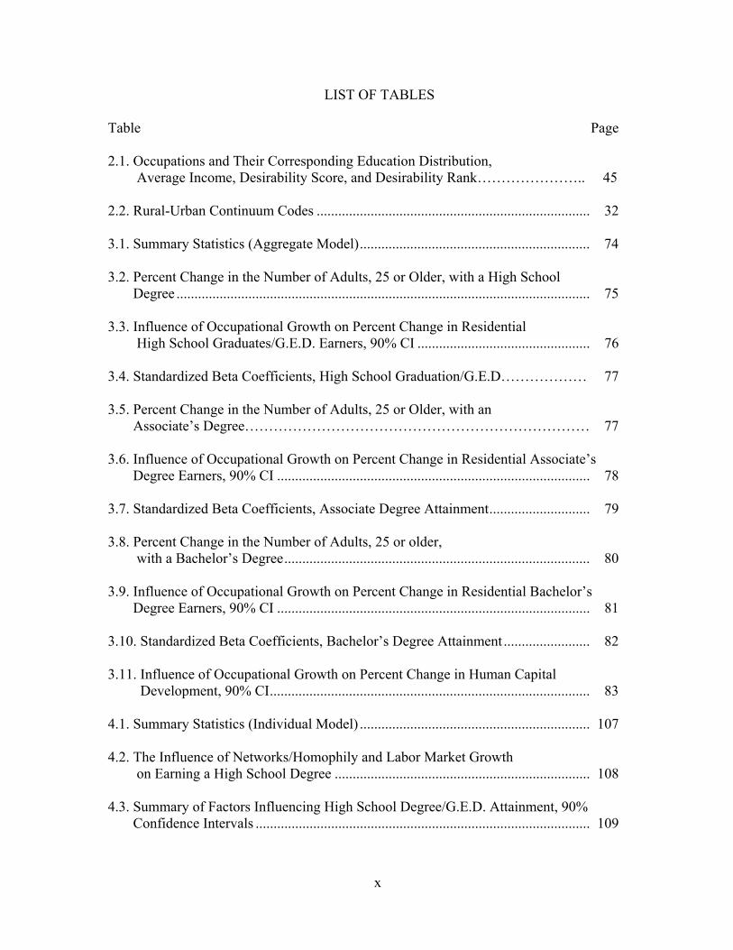
2.1. Occupations and Their Corresponding Education Distribution, Average Income, Desirability Score, and Desirability Rank………………….. 45 2.2. Rural-Urban Continuum Codes ............................................................................ 32

3.1. Summary Statistics (Aggregate Model) ................................................................ 74

3.2. Percent Change in the Number of Adults, 25 or Older, with a High School Degree ................................................................................................................... 75 3.3. Influence of Occupational Growth on Percent Change in Residential High School Graduates/G.E.D. Earners, 90% CI ................................................ 76 3.4. Standardized Beta Coefficients, High School Graduation/G.E.D……………… 77

3.5. Percent Change in the Number of Adults, 25 or Older, with an Associate’s Degree……………………………………………………………… 77 3.6. Influence of Occupational Growth on Percent Change in Residential Associate’s Degree Earners, 90% CI ....................................................................................... 78 3.7. Standardized Beta Coefficients, Associate Degree Attainment ............................ 79

3.8. Percent Change in the Number of Adults, 25 or older, with a Bachelor’s Degree ..................................................................................... 80 3.9. Influence of Occupational Growth on Percent Change in Residential Bachelor’s Degree Earners, 90% CI ....................................................................................... 81 3.10. Standardized Beta Coefficients, Bachelor’s Degree Attainment ........................ 82

3.11. Influence of Occupational Growth on Percent Change in Human Capital Development, 90% CI ......................................................................................... 83 4.1. Summary Statistics (Individual Model) ................................................................ 107

4.2. The Influence of Networks/Homophily and Labor Market Growth on Earning a High School Degree ....................................................................... 108 4.3. Summary of Factors Influencing High School Degree/G.E.D. Attainment, 90% Confidence Intervals ............................................................................................. 109

xi

Table Page

4.4. The Influence of Networks/Homophily and Labor Market Growth on earning an Associate’s Degree ............................................................................................... 110 4.5. Summary of Factors Influencing Associate’s Degree Attainment, 90% Confidence Intervals................................................................................................................ 111 4.6. The Influence of Networks/Homophily and Labor Market Growth on earning a Bachelor’s Degree ................................................................................................ 112 4.7. Summary of Factors Influencing Bachelor’s Degree Attainment, 90% Confidence Intervals................................................................................................................. 113 4.8. Summary of Factors Influencing Degree Attainment, 90% Confidence Intervals................................................................................................................ 114

1

CHAPTERI

INTRODUCTIONANDLITERATUREREVIEW

Currently, there is a plethora of studies addressing human capital investment within the

context of education. Much of the literature bridging local labor market conditions and

education outcomes focuses on high school dropout rates and college enrollment in relation

to unemployment rates and local wages. Historically, few studies have attempted to link

growth within specific labor markets to the type of degree residents earn, i.e., a high school

degree/G.E.D., an Associate’s, and a Bachelor’s. In other words, do potential degree earners

consider the types of jobs available to them when making decisions concerning their human

capital investment? Are students more likely to pursue a college degree if there has been

substantial growth within occupations requiring a college education? Corollary, are they less

likely to pursue a college degree if employment growth has primarily occurred with

secondary market occupations? What about high school graduation and earning an

associate’s degree? Are students more likely to graduate high school if locally available jobs

only require a high school degree? Are they more likely to finish high school if locally

available jobs require an Associate’s or Bachelor’s degree?



theories. To gain an understanding of how growth in multiple labor market tiers and various

occupation types influence local human capital development as well as students’ decisions to

invest in their own human capital; two modeling approaches are utilized. First, the

association between local employment growth by labor market tier and aggregate human

capital development is evaluated. Here, the percentage gain in counties stock of high school

2

graduates, Associate’s degree earners, and Bachelor’s degree earners between 2000 and 2014

is regressed against employment gains within primary, mid-level, and secondary labor

markets within the same timeframe. Second, occupations found to significantly influence

local human capital development are transferred to models gauging the educational

attainment of individual respondents. In both sets of models, “educational attainment” is

measured by the type of degree earned as a means of testing whether growth in primary,

secondary, and mid-level labor markets have measurably different magnitudes of effect on

the type of degree earned.

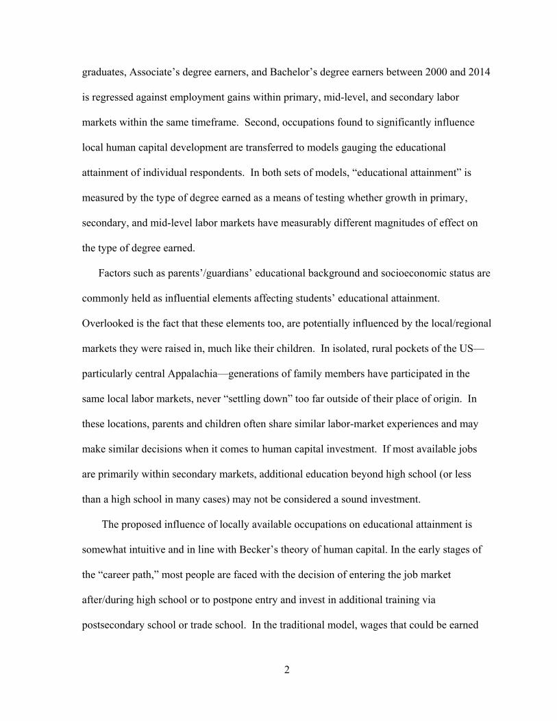
Factors such as parents’/guardians’ educational background and socioeconomic status are

commonly held as influential elements affecting students’ educational attainment.

Overlooked is the fact that these elements too, are potentially influenced by the local/regional

markets they were raised in, much like their children. In isolated, rural pockets of the US—

particularly central Appalachia—generations of family members have participated in the

same local labor markets, never “settling down” too far outside of their place of origin. In

these locations, parents and children often share similar labor-market experiences and may

make similar decisions when it comes to human capital investment. If most available jobs

are primarily within secondary markets, additional education beyond high school (or less

than a high school in many cases) may not be considered a sound investment.

The proposed influence of locally available occupations on educational attainment is

somewhat intuitive and in line with Becker’s theory of human capital. In the early stages of

the “career path,” most people are faced with the decision of entering the job market

after/during high school or to postpone entry and invest in additional training via

postsecondary school or trade school. In the traditional model, wages that could be earned

3

throughout the duration of the training period (often years) are forfeited in favor of higher

wages later. It follows, if high-skilled occupations are scarce both locally and within a

[subjectively] reasonable commuting distance, financing additional training and/or education

may be viewed as a bad investment by recent graduates. As such, a higher proportion of

graduates may enter the labor market immediately after high school graduation—or during

high school—compared to areas with a more diverse labor market or where more high-skill

occupations are available.

In addition, the proposed influence is an extension of Bozick’s research on the

warehouse hypothesis linking perceived job opportunities to college enrollment, though with

a few caveats. Bozick’s analysis focuses on the propensity of recent high school graduates to

enroll in college based on the unemployment rate and the volume of locally available jobs

that do not require a college degree. Whereas Bozick’s study examines unemployment and

job availability during the year that high school seniors graduate, this study examines

employment growth by labor market tier and occupation type over a period of 10 years;

beginning when respondents were sophomores in 2002, and ending in 2013—when

respondents would have been roughly 25-27 years old. Additionally, this study examines the

likelihood of graduating high school and earning an Associate’s or Bachelor’s degree based

on perceived job opportunities as opposed to college enrollment.

This study attempts to answer six questions. 1. Does employment growth in primary

market occupations stimulate growth in the number of high school graduates and college

degree earners? 2. Given (1) is verified, how does the impact of employment growth in

primary occupations compare to the impact of growth in lower-tiered occupations? 3. Does

employment growth in primary market occupations influence the probability of respondents

4

graduating high school and/or earning a college degree? 4. Given (3), how does the impact of

employment growth in primary occupations compare to the impact of growth in lower-tiered

occupations? 5. Does employment growth in primary, mid-level, and secondary market

occupations influence the high school graduation and/or earning a degree when controlling

for network/homophily effects? 6. Do occupations illustrated to affect growth/decline in the

number of degree earners translate to an increased/decreased probability of earning a degree

among individuals?

Academic literature thus far has not linked labor markets to educational outcomes in the

manner I am proposing. Often, the causal relationship addressed is usually the opposite, i.e.,

the role of educational outcomes on career choices and/or local labor markets. To ascertain

the influence of local/regional labor markets on educational outcomes, both human capital

and dual labor markets will be guiding theories; the former for its emphasis on incentives, the

latter for its structural account of the American labor market. Due to data and theoretical

limitations, however, this study does allow for the assessment of individual mechanisms—

outside of background factors such as parents’ socioeconomic status and level of education—

which may influence students’ decisions on their human capital investment. Here, the

primary independent variables of interest focus on change in aggregate employment

opportunities within an 8 to 10 year time frame. As such, individual mechanisms associated

with occupational and educational outcomes—parental involvement in students’ education,

network ties leading to information about local employment opportunities, cultural capital,

etc.—will not be addressed in this analysis.

The remainder of this chapter is laid out as such; section 1 identifies key literature

pertaining to human capital theory and the use of token measures of labor-market health—

5

such as business-cycles—as explicates of high school graduation rates and college

enrollment rates. Section 2 details literature on dual labor market theory as a response to

neoclassic economic models of human capital. Section 3 highlights literature on the role of

networks/homophily on education outcomes. Section 4 discusses the limitations of Human

Capital and Dual Labor Market Theories in their assessment of educational outcomes and

what it means for the current study. The final section provides a roadmap for the dissertation.

HumanCapital,LaborMarkets,andEducationalOutcomes

Human Capital Theory falls under the umbrella of Ration Choice Theory which

characterizes humans as self-interested (though, not necessarily selfish) rational actors whose

decisions are governed by “utility maximization” (Hechter & Kanazawa, 1997; Green &

Shaprio, 1994; Little, 1991). Individuals are assumed to have a set of interests/goals for

which they evaluate appropriate courses of action to obtain. Agents then rank each course of

action on the perceived ability to maximize their preferences. Human capital theory is

moreorless Rational Choice Theory applied to the development of advanced/nuanced skill-

sets to maximize wages, benefits, etc. and/or advance in one’s current occupation. In general,

human capital is accrued in the same matter as other forms of capital; most require some

degree of monetary or time investment, with the general expectation of returns exceeding the

initial cost. Human beings invest in their health, education, vocational training, etc. with the

expectation of greater returns on their investment over the course of their lifetimes (Becker,

1964; Shultz, 1961). Within the context of education, students “invest” in additional

education to develop a more refined skill set with the expectation that their future earnings

will offset the cost of training as well as wages lost during the training process. In situations

where; A) there are very few locally available high-skill occupations; or B) recent graduates

6

are not embedded in networks containing information about available high-skill, high-wage

occupations; pursuing additional education/training may not be seen as an appropriate avenue

for maximizing income or job satisfaction.

Human capital theory is pervasive in studies of education. Much of the literature on

human capital investment focuses on the influence of markets on high school dropout rates

(Rees & Mocain, 1997; Black, McKinnish, & Sanders 2005; Duncan, 1965; Rumberger,

1983; Neumark & Wascher, 1995; Goldin & Katz, 1997), college attendance (Betts &

McFarland, 1995; Fuller, Manski, & Wise, 1982; Manski & Wise, 1983; Becker, 1994;

Schultz, 1961; Perna, 2000), choice of college major (Altonji, Blom, & Meghir, 2012; Song

& Glick, 2004; Davies & Guppy, 1997) and returns to education (Becker, 1964; Shultz,

1961; Kane & Rouse, 1995; Morgenstern, 1973; Mincer, 1958; Blaug, 1972; Rouse, 2005;

Roksa & Levey, 2010). In addition, economic boom and bust cycles have also been linked to

high school dropout rates and college enrollment rates (Bedard & Douglas, 2007; Light,

1996). For the purposes of this study, the incentives for finishing high school and/or earning

a college degree will be the focus.

HighSchoolDropouts

The consequences of not finishing a high school degree are immense; hence non-

completion seems counter-intuitive in the contexts of human capital theory. Compared to

people with a high school degree, dropouts experience lower lifetime earnings (Rumberger,

1987; Rouse, 2005; Sum, Khatiwada, & McLaughlin, 2009), contribute significantly less to

the tax base (Rouse, 2005; Sum, Khatiwada, & McLaughlin, 2009; Catterall, 1987), are more

dependent on social welfare (Rumberger, 1987; Catterall, 1987; Levin, 1972) and more likely

to be unemployed (Rumberger, 1987; Sum, Khatiwada, & McLaughlin, 2009; Rouse, 2005;

7

Catterall, 1987). On a related note, Brenner (1976) found that unemployed persons are more

likely to experience poor mental and/or physical health, increased mortality, suicide, and

admission to state mental hospitals. Indirectly, this suggests earning a high school degree not

only increases employability, lifetime earnings, etc.; but also, increases overall health as

well. Despite negative outcomes routinely associated with dropping out of high school, both

labor market conditions and long-term wage increases have been illustrated as influential on

high school dropout rates.

Using reconstructed data from the 1960 Census, Duncan (1965) examined the

relationship between high school graduation and unemployment rates from 1902 to 1956.

She found that during periods of high unemployment, a larger percentage of students

remained in school. When unemployment was low, high school completion rates decreased.

Partitioning out high school completion rates by race and gender, Rumberger (1983) found

both black and Hispanic students were more likely to dropout when local unemployment

rates were low. However, white males where more likely to dropout during periods of high

unemployment. When queried as to why they left school, nearly a quarter of male

respondents cited “economic reasons” as the main catalyst for dropping out. Comparatively,

15 percent of female respondents left school for early entry into the labor force. Noted by

Black et al (2005), the Duncan study suffers from variable omission bias (does not include

family background variables) and the Rumberger study does not account for local labor

market characteristics other than unemployment.

Utilizing panel-data estimation techniques and district-level data to account for variable

omission bias and unobserved environmental characteristics, Rees and Mocan (1997)

illustrated that both White and Hispanic students are less likely to leave school when local

8

unemployment rates are high. In fact, a 1 percent increase in New York State’s

unemployment rate was associated with a 2 percent decrease in district dropout rates. This

effect remained significant even when controlling for factors such as teachers’ education and

years of experience. Black students, however, are more likely to leave school when economic

conditions are turbulent (suggestions as to why was not given). Though Rees and Mocan

adjust for variable omission bias and include locational characteristics, they do not account

for the variation of industries within local labor markets.

Three studies address the effect of wage increases in low-skill occupations on high

school completion rates. Neumark and Wascher (1995) used a conditional logit model to

analyze state-year data from 1977 to 1989. They found that increases in states’ minimum

wages significantly increases high school dropout rates and is inversely related to the

proportion of teens that are neither employed nor enrolled in school. Wages in the

manufacturing industry have also been illustrated as influential on high school completion

(Goldin & Katz, 2008), though results may not be applicable to present markets given the

dated time frame of the study (1910 to 1940). Black, McKinnish, and Sanders (2005)

provide a more contemporary study of the coal industry in Pennsylvania and Kentucky

during the 1970s and 1980s. They found that the high wages accompanying the coal boom

of the 1970s decreased high school enrollment rates in coal-producing counties. Corollary,

high school enrollment increased during the coal bust of the 1980s. In addition, they

illustrated that a 10 percent increase in wages for low-skill labor decreased high school

enrollment by 5 to 7 percent. Though studies by Goldin and Katz (2008) and Black,

McKinnish, and Sanders (2005) take wage differentials and industry-type into account;

9

examining a single industry is too restrictive—results are not applicable to other industry

types.

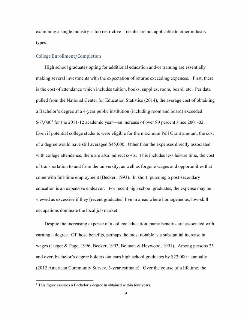
CollegeEnrollment/Completion

High school graduates opting for additional education and/or training are essentially

making several investments with the expectation of returns exceeding expenses. First, there

is the cost of attendance which includes tuition, books, supplies, room, board, etc. Per data

pulled from the National Center for Education Statistics (2014), the average cost of obtaining

a Bachelor’s degree at a 4-year public institution (including room and board) exceeded

$67,0001 for the 2011-12 academic year—an increase of over 80 percent since 2001-02.

Even if potential college students were eligible for the maximum Pell Grant amount, the cost

of a degree would have still averaged $45,000. Other than the expenses directly associated

with college attendance, there are also indirect costs. This includes less leisure time, the cost

of transportation to and from the university, as well as forgone wages and opportunities that

come with full-time employment (Becker, 1993). In short, pursuing a post-secondary

education is an expensive endeavor. For recent high school graduates, the expense may be

viewed as excessive if they [recent graduates] live in areas where homogeneous, low-skill

occupations dominate the local job market.

Despite the increasing expense of a college education, many benefits are associated with

earning a degree. Of those benefits, perhaps the most notable is a substantial increase in

wages (Jaeger & Page, 1996; Becker, 1993, Belman & Heywood, 1991). Among persons 25

and over, bachelor’s degree holders out earn high school graduates by $22,000+ annually

(2012 American Community Survey, 3-year estimate). Over the course of a lifetime, the

1 This figure assumes a Bachelor’s degree in obtained within four years.

10

additional income translates to an estimated $660,0002 more than high school graduates.

Other benefits of a college degree include a more fulfilling work environment, better health

and health care, and a decreased likelihood of unemployment (Baum & Payea, 2004; Bowen,

1996; Leslie & Brinkman, 1988). The benefits of a college education are not limited to the

bachelor’s degree, as several studies have indicated significant increases in pay among

Associate’s degree earners (Kane & Rouse, 1995; Belman & Heywood, 1991; Jaeger & Page,

1996; Marcotee et al, 2005). In addition, Kane and Rouse (1995) found that community

college attendees who did not obtain their Associates degree still out earned those without a

college education by 10 percent. The benefits of a degree are not limited to individuals.

Societal benefits include an increased tax base, lower incarceration rates, higher voter

turnout, increased blood donations at local clinics, decreased likelihood of smoking, and a

locally reduced strain on social welfare programs (Baum & Pyea, 2004, Bowen, 1996).

Other than studies which examine economic returns to a college degree, there is very

little research connecting labor market conditions to obtaining an Associate’s or Bachelor’s,

though several examine its link to college enrollment. Morissette, Chan and Lu (2014), for

example, found that college enrollment in Canada was linked to global oil prices from 2001

to 2008; as global oil prices decreased, college enrollment increased. As with research on

high school completion, several studies link college enrollments to unemployment rates

(Betts & McFarland, 1995; Hillman & Orians, 2013; Pennington, McGinty, & Williams

2002; Bozick, 2009). Largely, an increase in unemployment coincides with an increase in

college enrollment, particularly at community colleges. Indeed, increased unemployment

rates have also been illustrated to influence the decision to enroll part-time or full-time

2 30 years of employment with an additional $22,000 per year.

11

(Stratton, O’Toole & Wetzel, 2004). Utilizing the warehouse hypothesis—which holds that

students are more likely to remain in school when labor market conditions are unfavorable

and more likely to exit school for employment when market conditions are favorable—

Bozick (2009) illustrated that recent high school graduates where more likely to enroll in

college when unemployment was high and the availability of jobs that do not require a

Bachelor’s degree is low. Corollary, students were more likely enter the job market when

unemployment was low and the number of available jobs that do not require a Bachelor’s

degree is high.

DualLaborMarketTheory

During the 1960s, government-funded occupational training programs were sprouting up

in central cities to combat what was perceived as “supply-side” deficiencies within the

workforce (Doeringer et al, 1972) as part of a Lyndon Johnson’s “War on Poverty.” The

consensus, and a view in line with human capital theory, was that regionally high

unemployment and underemployment rates were the byproduct of an uneducated and

unskilled workforce, thus making them “unemployable.” In response, the Concentrated

Employment Project (CEP) was established to aid government programs in educating and

training workers to increase “manpower,” thus producing more employable workers and

reducing underemployment and poverty, or so the logic went. In an 18-month study of a

CEP program established in Boston, Doeinger et al. (1972) found that high unemployment

was not related to the employability of the workforce so much as the quality of the

occupations they had access to. Most trainees who participated in the CEP-sponsored

program were placed in low-wage occupations that did not offer a career ladder. As such,

many employees quit their jobs.

12

Stemming from neoclassical economic theories’ inability to explain occupationally-

based differences in labor market experiences, skepticism of human capital theory’s efficacy

became prevalent. Additionally, human capital theory did not address occupational clustering

or segregation as well as wage differentials across racial, gendered, and spatial divides

(England, 1982; Poire, 1972, 1975; Zellnar, 1972; Weisskoff, 1972; Gordon, 1971). In short,

human capital theory was criticized for its failure to take structural processes into account.

Instead of focusing on differences between occupations and the markets they are embedded

in, the primary focus of human capital theory is investment in one’s own skill set—people

who are unemployable or have low-skill jobs have not developed the expertise adequate to

obtain a quality occupation. Subsequently, and in response to the deficiencies of neoclassical

economic theories, Dual Labor Market/Labor Market Segmentation Theory was developed.

Born from the Doeringer and Piore’s (1971) research on internal labor markets, dual

labor market theory conceptualizes the American labor market as divided into good jobs and

bad jobs, each type clustering together to form two separate markets. Good jobs are located

in the primary market while bad jobs are located in the secondary market. Jobs within the

primary market share several characteristics including “high wages, good work conditions,

employment stability, chances of advancement, equity, and due process in work rules”

(Doeringer & Piore, 1971). In contrast, the secondary market consists of jobs that: are low

paying, unstable, offer limited benefits (if any), provide a poor working environment, offer

little chance of advancement, and high turnover.

Regarding the primary market, early proponents of dual labor market theory realized

many occupations fell somewhere in between primary and secondary. As such, the primary

market was eventually broken up into upper and lower tiers (Piore, 1973, 1975; Osterman

13

1975), each with their own unique set of characteristics. Upper tier occupations offer more

job control and autonomy; are often more complex in nature; “encourage and require

creative….self-initiating characteristics;” are less routinized; have higher turnover rates due

to advancement; and are more “closely related to formal education and personal

achievements” (Harrison & Sum, 1979; Reich, Gordon, & Edwards, 1973; Hudson, 2007).

Examples of upper tier occupations include management, professor, doctor, lawyer, etc.

Lower tier jobs within the primary sector are “more routinized, and encourage personality

characteristics of dependability, discipline, responsiveness to rules and authority, and

acceptance of a firm’s goals” (pg. 360. Reich, Gordon, & Edwards, 1973). In addition,

turnover is slow in low-tier occupations as employees become “locked in a career pattern” or

a specific internal market (Doeringer & Piore, 1971; Anderson, Butler, & Sloan, 1987).

Some examples of low-tier occupations within the primary market include factory work,

clerical work, and most blue-collar occupations in general.

Another characteristic of dual labor market theory is the limited mobility to move from

the secondary to the primary market (Doeringer & Piore, 1971). In many cases, “work” is

not the primary focus of persons employed in the secondary market. The income derived

from these occupations could be supplemental, as employees’ households may have a

primary market breadwinner (Hudson, 2007). Other research suggests that workers initially

employed is in the secondary labor market will continue to work in this sector throughout the

course of their life (Gordon, 1972; Piore, 1970; as cited in Hudson, 2007).

PreviousResearch

As with human capital theory, much of the literature on dual labor market theory has

been mixed. Supportive studies focus on the segregated nature of the labor market (Oster

14

1979; Kaufman, Hodson, & Fligstein, 1979; Gittleman & Howell, 1995); differences

between primary and secondary markets (Graham & Shakow 1990); and groups that are

more frequently segregated to occupations within the secondary market--specifically women,

immigrants, and nonwhites (Boston, 1990; Zellnar, 1971; Weisskoff, 1972; Hiebert, 1991;

Sakamoto and Chen, 1991; Sakamoto & Powers, 1995; Leontaridi, 1998). Studies more

critical of dual labor markets cite the theories ambiguity (Heckman & Hotz, 1986;

Leontaridi, 1998) and question the “limited mobility” tenant (Griffin, Kalleberg, &

Alexander, 1981; Anderson, Butler, & Sloan, 1987).

Several studies have implemented a factor analysis approach to illustrate distinct

groupings of occupations based on a number of characteristics. Analyzing 83 3-digit 1960

Census code industries, Oster (1979) found evidence supporting dual structuralism within the

job market. Industrial characteristics associated with the primary markets—characteristics

such as a concentration of firms with sales over $100 million, total industrial assets, and total

industrial income—significantly “loaded” to create a single factor. An additional PDF

(population probability density function) test both confirmed and partitioned 55 of the 83

industries into the secondary (or peripheral) market and 28 into the primary (or “core”)

market. Using a combination of both factor and cluster analysis, Kaufman and company

(1979) classified the American labor market into 16 distinct sectors. Dimensions used to

distinguish differences between sectors included concentration (the extent to which industries

are dominated by a handful of companies), size, capital/labor intensity, foreign involvement,

government intervention (i.e., regulation), profit, autonomy, unionization, productivity, and

growth. In an assessment of 621 occupations, Gittleman and Howell (1995) grouped

15

occupations into 6 job categories using a cluster analysis. Here, occupations were clustered

based on 17 measures of job quality.

Studies of the American labor market have also highlight gender- and race-based

occupational segmentation (Zellnar, 1972; Weisskoff, 1972; Hiebert; 1991; Leontaridi,

1998). In 1900, roughly one-third of employed women were concentrated into a single

occupational category, namely “private household worker” (Weisskoff, 1972). As of 1969,

the distribution of women across occupations increased though the “type” of occupations

women were concentrated in were similar. Utilizing 1960 census data, Zellnar (1972)

demonstrated that roughly 50 percent of employed women held occupations in which they

made 80 percent or more of the employees. Only 2 percent of employed men where in these

occupations. Indeed, 90 percent of men held jobs where they made up more than a third of

all employees. The effects of this segmentation process were shown to drive down the

overall wages of women.

Regarding immigration, studies suggest many immigrant workers form and participate in

enclave markets and/or remain in the secondary labor market (Wilson & Portes, 1980; Mata

& Pendakur, 1999). It is not uncommon for immigrants new to the U.S. labor market to start

their own small businesses and employ other immigrants (Wilson & Portes, 1980). Mata &

Pendakur (1999) suggest that immigrant entrepreneurship may be a response to the nature of

a dual labor market economy. Due to education and/or language barriers, immigrants may

choose self-employment over working in the secondary labor market. Indeed, Alcobendas

and Rodriguerz-Planas (2010) show that immigrants to Spain are disproportionately funneled

into the secondary labor market despite the skill and education of the workforce. The authors

suggest that several occupations requiring a high degree of education also require some form

16

of certification—certification which may be specific to the host country. As such, many

immigrants choose self-employment or seek work in immigrant-owned businesses.

Previous studies also show minorities tend to be segregated to the secondary labor

market (Rosenberg, 1976 as cited in Dickens and Lang 1985; Carnoy, & Rumberger 1980;

Dickens & Lang, 1985; Boston, 1990; Hudson, 2007). Rosenberg (1976), Carnoy, and

Rumberger (1980) found that minority workers are more likely to begin their careers in the

secondary labor market and also more likely to remain there compared to whites. Boston

(1990), shows that 58.8 percent of black men and 47.3 percent of black women were

employed in the secondary sector in 1983—a time when all workers in the secondary labor

market accounted for a quarter of all citizens in the labor force. Extrapolating from a series

of studies, Dickens and Lang (1985) hold that there are barriers to primary sector jobs for

minorities that do not exist for whites. Hudson (2007), using a multinomial hierarchical

modeling technique, found that both black men and women, noncitizen Hispanic men and

women, and Native American men are more likely to be employed in the secondary labor

market.

Studies examining the spatial dimension of dual labor market theory tend to focus on

“spatial mismatch,” or what occupations are spatially accessible to whom. Dubbed the

Spatial Mismatch Hypothesis (SMH), researchers have utilized the theory to explain income,

opportunity, and employment differentials between urban and suburban spaces; primarily

focusing on inner-city poverty among African Americans (Kain, 1992; Ihlanfeldt & Sjoqusit,

1998). McLafftery and Preston (1992), for example, found that African American and

Hispanic women in northern New Jersey are more dependent on public transportation and

thus have poorer spatial access to jobs compared to white women. Latina women were shown

17

to have better access to jobs within the local labor market but also earned considerably less

than African American and White women. This suggests that there was not a lack of

occupations in the area, but a lack of decent-paying occupations. Doeringer et al (1972) also

concluded that the number of occupations available in urban centers was not an issue so

much as the lack of well-paying jobs. Venti (1975) reach similar conclusions in his study of

welfare recipients in Massachusetts.

Research critical of dual labor market theory cites its ambiguity and the supposed

inability of workers in secondary markets to move to primary markets. Analyzing labor

market earnings and inequality among Panamanian males, Heckman and Hotz’s (1986)

income model of persons above the poverty line did not explain earnings of the poor, even

when controlling for selection bias. They cite a number of reasons why their results do not

support to dual labor market theory including: the potential existence of two or more sectors

in the labor market, yet all are lumped into “primary” or “secondary’; workers as utility

maximizers rather than earning maximizers; the inability to separate the cost associated with

moving between secondary and primary sectors from barriers to entry; and false

distributional assumptions. The authors conclude that in order to test for the existence of a

dual market, a “true functional form of the earnings equation under the hypothesis of no

dualism” is assumed to be known (pg. 529). As such, Heckman and Hotz hold dual labor

market theory as untestable.

Leontaridi (1998) also cites the presupposed existence of two labor sectors as an inherent

weakness of dual labor market theory. Extrapolating from previous studies, the author

concludes that while the use of cluster and factor analysis solves the issue of “a priori

segment determination,” the number of proposed sectors resulting from these studies are

18

dependent on both the number and type of variables used. This suggests there is not an

agreed-upon methodology to test dual labor market theory.

Regarding mobility between secondary and primary sectors, several studies have found

that rigid barriers between markets do not exist.3 Anderson, Butler, and Sloan (1987), using

the Panel Study of Income Dynamics, develop indices of job traits which are used to

characterize occupations as good or bad. Their results indicate that job groupings based on

jobs traits (wages, layoffs, unionized, unemployment, etc.) did not conform to dual labor

market theory. Given that occupations could not be clustered based on their characteristics,

rigid barriers between sectors do not exist. In a previous study examining the determinants

of early labor market entry; Griffin, Kalleberg, and Alexander (1981) found “considerable

inter-sectoral mobility” and few characteristic differences in the employees working in each

sector. Mayhew and Roswell (1979) and McNabb (1987) found that the education of

workers was highly correlated with their place in the “occupational hierarchy,” thus the

existence of rigid barriers between primary and secondary sectors are questionable.

TheInfluenceofPeersonAcademicAchievement

For well over half a century, the role of peers on students’ educational, occupational, and

long-term life outcomes has been a topic of interest among education researchers. Much of

the literature on peer-group effects has focused on the role of social cliques as a means of

establishing class boundaries (Hollingshead, 1949), peer influence on academic performance

(Coleman, 1961; Hanushek et al, 2003; Calvo-Armengol et al 2009; Hoxby, 2000;

Zimmerman, 2003; Angrist & Lang, 2002), student tracking (Duflo, Dupas, & Kemer, 2011);

3 For additional material, see Psacharopoulos (1978), Mayhew and Rosewell (1979), McNabb (1987), Leigh (1976), and Schiller (1977).

19

the likelihood of dropping out of high school (Cairns, Cairns, & Neckerman, 1989; Jimerson

et al, 2000:Carbonaro & Workman, 2013, 2016); selection bias in peer-effect studies

(Zimmerman, 2003; Sacerdote, 2001; Hoxby, 2000); college major (Sacerdote, 2001); and

student aspirations (Haller & Butterworth, 1960; Alexander & Campbell, 1964; Cuncan,

Haller, & Portes, 1968; Carbonaro and Workman, 2016; Martin, 2009).

SocialCliquesandAcademicAchievement

Regarding social cliques, in a field study of 735 adolescents between the ages of 13 and 18

residing in a Midwest community, Hollingshead (1949) found that teenager’s behaviors were

linked to their position with the towns stratified social structure. The youths of Elmstown,

Illinois predominantly interacted with and dated those within the same social strata, with the

occasional deviation. In addition, Hollingshead noted that students within the lower strata

generally did not engage in any social and/or community events; high school students did not

attend athletic events, join school clubs, etc. In short, youths and their families within the

lower strata did not have strong ties to their community.

Studies have generally been mixed on the influence of peers when it comes to students’

academic achievement. Some illustrate a connection between peer groups and achievement

as early as elementary and middle school. Utilizing a series of models that control for

student, school, and school-by-grade fixed effects, Hanushek et al (2003) illustrated that peer

achievement among 3rd through 6th grade students had a positive influence on students’

achievement growth. Results indicated that a .1 standard deviation increase in peer

achievement leads to a .02 increase in student achievement. When the distribution of math

scores were parsed, results were similar, though students in the uppermost quartile were not

as responsive to peer achievement.

20

In a study of 3rd, 5th, and 7th graders enrolled in Boston’s Metco program, Angrist and

Lang (2002) found that lower-scoring Metco participants did not significantly influence the

reading scores of their non-Metco peers. On the other hand, they did find evidence of an

intragroup effect based on racial composition. Specifically, there was an inverse relationship

between the proportion of Metco students and the reading test scores of Non-Metco students

among minority girls. As the former increased, the latter decreased.

In a study which examined peer effects, teacher incentives, and student tracking in

Kenya; Duflo, Dupas, and Kemer (2011) found 1st graders who attended schools with an

achievement-based tracking system outperformed their peers at non-tracking schools.

Utilizing a unique experimental design, 60 randomly selected schools assigned students to

sections based on initial test scores on a standardized exam given at the beginning of the

academic year. The remaining 61 schools randomly assigned students to one of two sections,

regardless of their initial achievement. At the end of an 18-month period, 1st graders who

attended tracking schools scored4 .14 standard deviations higher than students in non-

tracking schools. One year later, the difference had increased to .16 standard deviations.

When examined by section, students in both tiers benefited from tracking, the bottom tier5

gaining .16 standard deviations and the upper tier gaining .19 standard deviations.

In a separate analysis of friendship networks, Calvo-Armengol, Patacchini, and Zenou

(2009) highlight the importance of peer influence on education outcomes. Using the Katz-

Bonacich measure of network centrality, the authors show a standard deviation increase

equates to an achievement gain of 7% of one standard deviation. It is worth noting, however,

4 Students were tested on language and mathematics. 5 Students scoring below the median were placed into the lower tier section. Those scoring above the median were assigned to the upper tier.

21

that parental education accounted for a gain of 17% of one standard deviation per unit

increase. Results of their study indicate that students’ location within friendship networks

has a significant impact on their educational outcomes, though the effect size is small.

Several studies have also indicated that peer influence plays a significant role in high

school graduation. A study of early school dropouts by Cairns, Cairns, and Neckerman

(1989) showed a positive correlation between students’ friendship networks during 7th grade

and leaving school by their junior year. Among both male and female cliques, there was a

positive association between dropping out school and having friends who had dropped out of

school. In a separate longitudinal analysis of high school dropouts, Jimerson and company

(2000) illustrated peer competence at age 16 influences students’ graduation status at age 19.

In fact, the Wilks’s Lambda score for peer competence was slightly higher than the score for

students’ academic achievement.

By themselves, these studies do not necessarily illustrate a peer effect on the probability

of graduating high school and/or dropping out. Instead, the results may illustrate students’

tendency to affiliate with those having similar academic aspirations. In a study carried out by

Carbonaro and Workman (2013), however, a distinction is made between types of friendship

networks; specifically, close and distant friendships. The authors conclude that while the

volume of close friendship ties is negatively associated with dropping out of school, the

characteristics of close friends did not influence the likelihood of dropping out. In contrast,

the characteristics of distant ties was positively associated with dropping out. A later study

by Carbonaro and Workman (2016) illustrated the characteristics of friends’ friends was at

least as strong of a predictor as friends’ characteristics on dropping out of school and

expectations of college enrollment. Here, a homophily effect would dictate that the

22

characteristics of close ties be more influential than those of distant ties, yet the works of

Carbonaro and Workman show that distant ties are at least as important as close ties.

SelectionBias

As one may infer from the studies covered so far, selection bias is a pervasive issue when

analyzing peer-influence on academic achievement, as it difficult to determine if the effects

are, in fact, due to the influence of peers, or merely a reflection6 between students and their

peer groups. In other words, students’ academic outcomes are not influenced by their peers

so much as students with similar aspirations are more likely to interact with each other.

Their associated outcomes may still be a product of individuals’ background factors such as

aspirations, interests, socioeconomic background, etc.

Results from several studies illustrate why homophily is so problematic when peer effects

are of concern. Early models of peer influence on educational and aspirational outcomes note

the effects are potentially overshadowed by homophily effects (Haller & Butterworth, 1960;

Alexander & Campbell, 1964; Duncan, Haller, & Portes, 1968). Additionally, many studies

highlight the proclivity of youths to befriend other youths who share similar characteristics,

such as race/ethnicity (Moody, 2001; Joyner & Kao, 2000), gender (Shrum, Creek, & Hunter,

1988), and behavior (Kandel, 1978; Cohen, 1977). In Kandel’s (1978) study of adolescent

friendships, for example, similarities in attitudes and opinions among youths were due to

friendship choice, not peer influence. Utilizing longitudinal data on 957 “best-schoolfriend

dyads,” the author illustrates students tend to “coordinate their choices of friends and their

behaviors…so as to maximize congruency within friendship pairs.” Dyads in which

members shared similar frequencies of marijuana use, political identification, educational

6 See Manksi (1993) for details.

23

aspirations, and “minor delinquent activities” were more likely to remain intact at the end of

the school year. Members of new dyads which formed during the school year also shared

similarities in recreational drug use, political leanings, educational pursuits, and delinquent

behaviors.

Flashman (2012) also links educational aspirations and achievement to changing

dynamics within friendship networks. In her study of high school students, results indicated

that high-achieving students were more likely to develop friendship ties with other high-

achieving students. Corollary, low-achieving students were more likely to develop ties with

low-achieving students. The link between educational achievement and choice of friends

remained significant after controlling students’ socioeconomic backgrounds, race/ethnicity,

and proximity to other students. Taken together, these studies illustrate a seemingly

endogenous relationship between student behavior and peer group influence.

Several methodological approaches have been implemented by scholars as a means of

isolating peer effects from homophily effects. Utilizing the Texas Schools Microdata Panel,

Hoxby (2000), for example, used two separate strategies for measuring peer effects in the

classroom, both of which control for school policies, school location, parental influence on

classrooms/schools, student tracking by achievement, and a series of other factors that may

introduce selection bias. The first strategy involved measuring the variation in adjacent

cohorts’ (groups who are in the same grade, in the same school, within the same academic

year) share of gender and racial groups. In the second approach, the author measures

idiosyncratic variation in achievement between student groups and tests whether classroom

variation in race and gender is correlated with the variation in achievement. Results

supported the “peer effect” hypothesis; students who were surrounded by high achieving

24

peers earned higher reading scores. A 1-point increase in peers’ test scores generated a .10 to

.55 increase in students’ test scores, depending on model specifications.

Studies by Zimmerman (2003) and Sacerdote (2001) attempt to control for the selection

bias, via quasi-experiments involving randomly assigned, first-year college roommates. In

both studies, the authors examined students’ achievement outcomes based on the

achievement of their roommates. Zimmerman found that students who were assigned high

achieving roommates earned a higher cumulative and first-semester GPA. Additionally,

results indicated “mid-level” achievers who shared a room with “low-level” achievers had

lower GPAs compared to their “mid-level” peers with middle and high achieving roommates.

Sacedote (2001) also found a link between freshmen GPAs and that of their roommates,

though there was not an association between roommates’ college majors or decisions related

to the job market. In both Zimmerman’s study of Williams College students and Sacedote’s

study of Dartmouth freshmen, students’ academic achievement was significantly influenced

by the achievement of peers, but the effect size was small.

LimitationstoHumanCapitalTheoryandDualLaborMarkets

Despite their usage in studies of educational attainment, human capital theory and Dual

Labor Markets are not without limits. In both instances, there is the assumption of rational

actions on the part of potential degree-seeking persons while neglecting several individual

mechanisms which may also hold sway on the decision to pursue a degree. Specifically,

background variables such as parents’ highest level of education, parents’ socioeconomic

status, parental involvement in children’s education, quality of home life, and cultural capital

have been routinely illustrated to influence educational outcomes. As such, these factors may

influence students’ interpretation of available job opportunities as well as their decisions

25

regarding human capital investment. It is entirely possible for students who grow up in areas

with an abundance of diverse occupations requiring an Associate’s or Bachelor’s degree to

opt out of college for employment at a local car dealership, product distribution center, etc.

based on information and/or expectations of their parents, close relatives, friends, and peer

groups. The fact that Human Capital Theory and Dual Labor Markets does not account for

this is limiting.

Several studies have illustrated parents’ education and income influences both their

children’s educational attainment and occupational outcomes (Jimerson, Egeland, & Teo,

1999; Halle et al. 1997; Luster, Rhoades, & Haas,1989; Davis-Kean, 2005). Utilizing the

1997 Child Development Supplement of the Panel Study of Income Dynamics, Davis-Kean

(2005), illustrated that parent’s education and income directly the educational expectations

they have of their children; hence indirectly affecting children’s reading ability as well as

their standardized math and reading scores. Additionally, Parent’s education and income had

a positive effect on parental warmth within the home environment which, in turn, has also

been linked to higher educational outcomes (Glasgow et al, 1997).

Dimaggio (1983) and Dimaggio and Mohr (1985) illustrate that cultural capital plays a

significant role in education. Measuring several dimensions of cultural capital (attitudes

towards the arts, cultural interests, etc.) on the academic performance of junior-year high

school students, Dimaggio (1983) found cultural capital had a positive effect on math,

English, and history grades among both male and females. In a latter study, Dimaggio and

Mohr (1985) found cultural capital to not only improve grades during high school, but to also

influence the likelihood of college enrollment. Additionally, cultural capital has also been

26

illustrated to facilitate entry into high-wage, high-skill, professional occupations (Egerton,

1997).

SynthesisoftheLiteratureandRoadMap

Research utilizing human capital theory illustrates a strong, positive association between

obtaining a high school and/or college degree and overall lifetime earnings, contributions to

the local tax base, lowered unemployment, decreased dependency on social welfare,

increased lifespan, better health and health care, and increased job satisfaction. In addition,

previous studies show the incentives for earning a high school degree/GED and/or pursue a

college education outweigh the loss of potential wages earned. Despite the incentives, many

persons reside in areas void of the types of jobs which provide the above-mentioned

incentives. What research has not addressed thus far is if and to what degree the composition

of local markets incentivizes residents to complete high school and/or earn a college degree.

While studies by Rees and Mocan (1997) and Rumberger (1983) include local employment

characteristics as predictors of high school dropout rates, they do not account for the

variation of local job opportunities. Whereas some studies have link high school dropout

rates and college enrollment to boom and bust cycles within specific industries (Black et al,

2005; Morissette, Chan & Lu, 2014), research thus far has not assessed the influence of local

job opportunities in multiple fields. In situations where; A) there are very few high-skill

occupations locally/regionally; or B) recent graduates are not embedded in networks

containing information about available high-skill, high-wage occupations; pursuing

additional education/training may not be an appropriate avenue for maximizing income or

job satisfaction.

27

Dual labor market theory holds that the American labor market is essentially divided into

good and bad jobs, the former found in primary markets and the later in secondary markets.

Characteristics of jobs within primary markets include high pay; benefits such as paid

vacation, sick leave, maternity leave, a retirement plan, etc.; and in most cases, are allocated

to persons with an advanced skill set. Jobs in the secondary market are characteristically the

exact opposite of jobs in the primary market (low pay, little or no benefits, does not require

an advanced skill set, etc.). Within the context of the US; women, minorities, and

immigrants are often relegated to the secondary labor market while white males occupy the

primary market. Perhaps most salient to this study, however, is that primary jobs may be

spatial inaccessibility, thus creating a roadblock to better incomes, increased benefits, etc.

As such, if most occupations within local/region markets are low paying jobs that do not

require an advanced skill set, fewer people within the area will have graduated high school

and/or earned a college degree. On the other hand, if high paying occupations are readily

accessible, people will be more likely to graduate high school and/or earn a degree.

Studies of peer influence on educational outcomes have routinely illustrated a positive

association between the “company students keep” and their academic performance, whether

the effect is a product of influence or homophily. Thus far, research addressing educational

outcomes has not compared/contrasted the influence on local labor markets to

network/homophily effects.

Lastly, several factors which are routinely associated with educational attainment and

occupational outcomes are not included in this analysis due to data limitations. Specifically,

data on cultural capital, individual mechanisms associated with parents’ SES and education

level, parental involvement with children’s education, and connections to persons with

28

information about potential job openings are not included in this study. As such, results

cannot speak to how the occupational background of parents effect the occupational

outcomes of their children; or how parental involvement in the local PTA and/or other school

activities affects their children’s educational prospects; or how network connections to

persons working in high-wage, high-skill occupations may or may not influence students to

earn a college degree so that they too may work within a similar industry; etc.

Roadmap

In Chapter II, I detail the methodological approach used to answer questions 1 through 5,

and introduce a “desirability” index, utilized to divide 23 American Community Survey

occupational categories into three distinct tiers. Chapter III details the results of tested

hypotheses which address the association between county-level employment growth by

occupation and counties’ stock of high school graduates/GED earners, Associate’s degree

earners, and Bachelor’s degree earners is assessed (hypotheses 1 and 2). In Chapter IV, I

address hypotheses 3 through 5. Occupations for which employment growth has a significant

impact on aggregate human capital growth are used in a second series of models examining

their influence on the educational outcomes of individual respondents. In the final chapter,

concluding remarks and a discussion of the study’s implications are provided.

29

CHAPTERII

METHODOLOGY



theories. To gain insight as to if and/or how labor market development influences local

human capital development via high school completion and/or earning postsecondary degree,

two modeling approaches are utilized. First, the influence of local employment growth with

primary, midlevel, and secondary labor markets and individual occupations on the volume of

high school graduates and college degree earners is assessed. Second, occupations found to

significantly influence local human capital growth are transferred to a model gauging the

educational attainment of individual respondents.

When assessing the role of local job markets on educational outcomes, it is important to

determine if growth in specific labor markets and occupations increase local human capital

development prior to examining their role on individual outcomes. For the sake of

parsimony, this study works under the assumption that if a specific job type does not generate

an increase in regional human capital, it will not sufficiently motivate young adults to

continue their education beyond necessity.7 For example—and speaking hypothetically—if

growth in sales occupations is associated with a proportional increase in the number of high

school degrees but does not influence growth in the number of bachelor’s degrees, then

growth in sales occupations will positively influence the probability of graduating high

school/earning a G.E.D., but have no bearing on postsecondary education. In this scenario, if

7 Preliminary models indicated occupations which did not influence aggregate human capital growth were nonsignificant predictors of individual outcomes.

30

a student wanted to pursue a career in sales, there would be no need to continue his/her

education beyond high school, thus growth in sales occupations would not encourage the

pursual of an Associate’s or Bachelor’s degree.

AggregateData

All data used to assess the influence of local employment growth by occupation on

educational gains is culled from the 2000 decennial census and the 2014 American

Community Survey (ACS) 5-Year Average. Specifically, data pertaining to 23 ACS

occupation types for all US counties are utilized. If accessible employment within these

occupations have a positive net effect on educational outcomes, then growth in the former

should coincide with growth in the latter. As such, change in earned degrees between 2000

and 2014 are regressed against employment change by labor market and occupation within

the same timeframe.

To measure growth over time in the dependent and independent variables, logged

differences were calculated such that:

Log(2014_var + 1) - Log(2000_var +1) = Log( ) = Log(difference_var),

where 1 is added to the total of each variable to prevent taking the log of 0 which is

undefined. In the unlikely event that the volume of high school graduates, college degree

earners, or employed persons in occupation “X” is 0 for in any given county, adding 1 to the

total will still reflect the absence as;

Log(0 + 1) = Log(1) = 0.

31

Occupations are measured at two levels of aggregation, the first of which is as defined by

the ACS. Second, all occupations are collapsed into three categories to reflect three distinct

job markets; more precisely, the primary job market, a midlevel job market, and the

secondary job market. As a means of collapsing occupations into one of three categories, a

“desirability” index was constructed using data pulled from the 2014 ACS microdata set,

provided by IPUMS. Data on individuals’ income and educational attainment was

standardized and summed across each occupation. Afterwards, an overall “desirability” score

was generated by averaging the summed values for each occupation and ranking them in

descending order. The top eight occupational categories were grouped together as tier-1 jobs

and are intended to reflect occupations in the primary job market; the seven middle

occupations represent the midlevel job market, and the bottom eight reflect the secondary job

market. Table 2.1 lists all occupational categories, their corresponding education

distribution, average income, desirability scores, and corresponding ranking. A brief

description of the occupations is provided in the appendix.8

In addition to employment changes by occupation, rural-urban continuum codes are also

included to test for differences in earned degrees between rural and urban counties. Also,

this will partially address differences between rural and urban labor markets, as the latter

tends to be less developed than the former. Maintained by the United States Department of

Agriculture (USDA), rural-urban continuum codes range from 1 to 9 and detail counties’

population size and proximity to a metro area. For the present analysis, the 2013 continuum

8 For a complete list of jobs within each occupation, the 2000 OCC codes can be found on the IPUMS website at https://usa.ipums.org/usa/volii/occ2000.shtml

32

codes are used as they are the most up-to-date. A detailed description of rural-urban

continuum codes is located in table 2.2.

Several race/ethnicity factors are included as control factors, as many studies have

identified a racially-based education gap (Ladson-Billings, 2006; Reimers, Cordelia, 1983;

Farkas, 2003). In addition, Rumberger (1983) and Rees and Mocan (1997) found that young

white, Hispanic, and Black men respond differently to local labor market conditions.

Previous labor market research has repeatedly illustrated that minority groups are

overwhelming excluded from primary market occupations and often reside in areas with

limited access to high-wage employment. As such, growth in the Asian, Black, Hispanic,

Native American, Pacific Islander, White, and Multiracial populations are accounted for.

Ideally, this will allow for better assessment of the relationship between local job markets

and human capital development.

Table 2.2. 2013 Rural-Urban Continuum Codes

ANoteonLaborMarkets

Historically, geographic proxies have often been used as a means of measuring local

labor market conditions, with the units ranging in size. Several studies have utilized

metropolitan statistical areas (MSAs) as the geographic boundaries of local labor markets.

2013 Rurality Code

Description

1 Metro - Counties in metro areas of 1 million population or more 2 Metro - Counties in metro areas of 250,000 to 1 million population 3 Metro - Counties in metro areas of fewer than 250,000 population 4 Nonmetro - Urban population of 20,000 or more, adjacent to a metro area 5 Nonmetro - Urban population of 20,000 or more, not adjacent to a metro area 6 Nonmetro - Urban population of 2,500 to 19,999, adjacent to a metro area 7 Nonmetro - Urban population of 2,500 to 19,999, not adjacent to a metro area 8 Nonmetro - Completely rural or less than 2,500 urban population, adjacent to a metro area 9 Nonmetro - Completely rural or less than 2,500 urban population, not adjacent to a metro area

33

For example, Blau, Khan, and Waldfogel (2000) showed that the marriage rate of women are

influenced by better female labor markets and worse male labor markets within 111 MSAs.

In an analysis of 72 MSAs, Marquis and Long (2001) illustrated that employers are more

likely to offer their employees health insurance at a higher contribution rate in tighter labor

markets with greater unionization. McCall (2001) also utilized MSAs as proxies for local

labor markets in her study of racial, ethnic, and gendered wage differences within

metropolitan labor markets.

A common issue brought up with the use of MSAs as proxies for local labor markets by

scholars is that they consist entirely of metropolitan areas. As such, the influence of labor

market conditions in more rural areas o cannot be inferred from empirical results. As means

of troubleshooting, researchers have often opted to use Public Use Microdata Area (PUMA)

units as geographic labor market proxies as they are smaller than MSAs and take commuting

patterns into consideration (Smith, 2012; Tolbert & Sizer, 1996). As such, results are more

relatable to areas of the country other than metropolitan spaces.

An additional method of measuring local labor market conditions—and implemented in

this study—is to use counties as the geographical unit of interest. Though they typically do

not constitute the entirety of a local labor market, the relatively smaller size of counties

compared to MSAs or PUMAs allows researchers to gauge the influence of market

conditions at a micro-level. Whereas employment opportunities may be plentiful in the east

end of town, this does not mean they are plentiful in the western portion. Within the context

of job opportunities and college enrollment, Borzick (2009) tied the high school location of

graduating seniors to county-level unemployment rates and the availability of jobs that did

not require a college degree. Thompson (2009) uses both county and state-level data to

34

examine the influence of the minimum wage on teenage employment. Overall, there is not a

single “go to” geographic unit that is used as a proxy for local labor markets.

DataforModelofIndividualOutcomes

To measure the effect of local/regional labor market conditions on high school

graduation, occupational employment shifts were measured at the county level over a period

of 10 to 14 years. Employment-by-occupation data was culled from the 2000 US Census and

the 2014 American Community Survey’s (ACS) 5-year estimate. As with the aggregate

models of human capital development, employment growth within primary, midlevel, and

secondary labor markets are the main independent variables of interest. Growth in individual

occupations, though of interest, is a secondary concern and their inclusion is more

exploratory in nature. While this study aims to assess the influence of primary markets

relative to midlevel and secondary markets, hypothesizing the influence of individual

occupations goes beyond the scope.

The primary dependent variables of interest were pulled from the 2002 Educational

Longitudinal Survey (ELS). Collected in four waves, ELS provides nationally representative

panel-data detailing students’ “trajectories from the beginning of high school into

postsecondary education, the workforce, and beyond.9” During the base year10 in 2002, ELS

surveyed high school sophomores, collecting data on where they went to high school, their

class schedules, grades, standardized test scores, relationships with peers and school faculty,

home life, etc. Respondents were surveyed again in 2004, 2006, and 2012 with questions

ranging from whether they graduated high school to their current job prospects. In total, ELS

9 www.nces.ed.gov/surveys/els2002 10 In 2002, the target population for first wave of surveys and interviews was limited to high school sophomores. During the second wave of surveys and interviews in 2004, additional high school seniors were included in the pool of respondents.

35

contains more than 8,000 variables pertaining to respondents’ education, high schools,

colleges, occupations, etc.

Several other measures were pulled from the ELS database to use as controls or to create

new variables of interest. Regarding the former, respondents’ demographics as well as their

parents’ educational attainment and income are routinely illustrated as influential on high

school graduation (Sewell & Shah, 1968; Dubow, Boxer, & Huesman, 2009; Roscigno,

1998; Astone & McLanahan, 1991; Krien & Beller, 1998). Specifically, underrepresented

minority students are less likely to graduate or earn a G.E.D. compared to their white peers

(Dubow, Boxer, & Huesman, 2009; Roscigno, 1998). In addition, parent’s education and

income are positively associated with students’ academic success (Sewell & Shah, 1968;

Astone & McLanahan, 1991); the higher the degree obtained or income earned, the more

likely respondents will graduate.

Six variables are used to gauge the influence of social networks/homophily on degree

attainment and labor market entry. Regarding the former, this study works with assumption

that respondents are more likely to graduate high school if they are surrounded by friends

and/or peers who plan to attend college after graduation, whether it’s a product of influence

or homophily. As for the latter, the line of reasoning is similar; respondents who are

surrounded by friends and/or peers who plan to enter the labor force after high school are less

likely to graduate and/or pursue a college degree.

Two variables are used to gauge how many of the respondents’ friends planned to attend

a community college or a 4-year university after high school graduation. For both measures,

four categories were provided: “None,” “Some of them,” “Most of them,” and “All of them.”

Here, it is important to note that these were the responses available to respondents, and that

36

data pertaining to these two survey items were not relabeled, categorized calculations based

on the proportion of respondents’ friends who planned to attend college, though it would be

preferable. In addition, two index variables are used to gauge respondents’ subjective views

as to the desire of others. Specifically, they measure whether respondents believe their ties

want them to go to college and/or get a job after high school graduation. Here, each index

variable is the sum of responses to six dichotomous variables, creating two measures ranging

from 0 to 6. Specifically, each survey item queries whether respondents felt as though they

were expected to continue their education or enroll in college by their mother, father, other

relatives, friend, favorite teacher, and school guidance counselor. A seventh survey item

pertaining to respondents’ favorite coach was also available, but not used since it severely

restricted the pool of respondents (a considerably small proportion of high school students

participate in sports compared to those who do not). Lastly, two school-level survey items

were included as additional measures of peer influence and/or homophily, each measuring

the percent of graduating seniors from the previous year11 who entered the labor

market/military or went to a 4-year university. All network/homophily survey items are

located in the appendix.

As with the aggregate model, the 2013 USDA rural-urban continuum codes12 are used to

gauge both the rurality and population size of counties. This will allow for the assessment of

high school graduation differences based on students’ proximity to urban areas.

11 The previous cohort would have graduated in 2003. Most first-wave ELS respondents would have been juniors at the time. 12 Rural-Urban continuum codes are located in table 2.2.

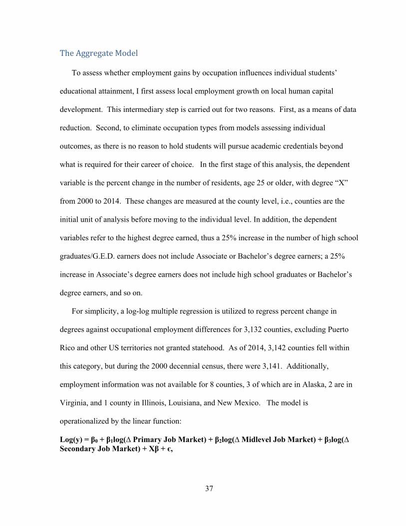
37

TheAggregateModel

To assess whether employment gains by occupation influences individual students’

educational attainment, I first assess local employment growth on local human capital

development. This intermediary step is carried out for two reasons. First, as a means of data

reduction. Second, to eliminate occupation types from models assessing individual

outcomes, as there is no reason to hold students will pursue academic credentials beyond

what is required for their career of choice. In the first stage of this analysis, the dependent

variable is the percent change in the number of residents, age 25 or older, with degree “X”

from 2000 to 2014. These changes are measured at the county level, i.e., counties are the

initial unit of analysis before moving to the individual level. In addition, the dependent

variables refer to the highest degree earned, thus a 25% increase in the number of high school

graduates/G.E.D. earners does not include Associate or Bachelor’s degree earners; a 25%

increase in Associate’s degree earners does not include high school graduates or Bachelor’s

degree earners, and so on.

For simplicity, a log-log multiple regression is utilized to regress percent change in

degrees against occupational employment differences for 3,132 counties, excluding Puerto

Rico and other US territories not granted statehood. As of 2014, 3,142 counties fell within

this category, but during the 2000 decennial census, there were 3,141. Additionally,

employment information was not available for 8 counties, 3 of which are in Alaska, 2 are in

Virginia, and 1 county in Illinois, Louisiana, and New Mexico. The model is

operationalized by the linear function:

Log(y) = β0 + β1log(∆ Primary Job Market) + β2log(∆ Midlevel Job Market) + β3log(∆ Secondary Job Market) + Xβ + є,

38

Where β 1 through β 3 represent one of three job markets, Xβ is the matrix-vector product

of control variables, and є is the error term. In addition, a second model assessing the

influence of individual occupations is included to determine if growth within specific fields

stimulate or reduce human capital development. The additional models take the form:

Log(y) = β0 + β1log(∆ Management) + β2log(∆ Business) + β3log(∆ Computer/Math) + β4log(∆ Architecture/Engineering) + β5log(∆ Life, Physical, & Social Sciences) + β6log(∆ Community & Social Services)+ β7log(∆ Legal Occupations) + β8log(∆ Education, Training, and Library Science) + β9log(∆ Arts & Entertainment)+ β10log(∆ Healthcare Practitioners)+ β11log(∆ Healthcare Technicians)+ β12log(∆ Healthcare Support) + β13log(∆ Protective Services) + β14log(∆ Food Preparation & Serving) + β15log(∆ Building & Grounds keeping & Maintenance) + β16log(∆ Personal Care) + β17log(∆ Sales) + β18log(∆ Office and Administrative Support) + β19log(∆ Farming, Fishing, and Forestry) + β20log(∆ Construction and Extraction) + β21log(∆ Installation, Maintenance, and Repair) + β22log(∆ Production) + β23log(∆ Transportation) + β24log(Rural Continuum) +Xβ + є,

Where β 1 through β24 are the independent variables of interest, Xβ is the matrix-vector

product of control variables, and є is the error term. Independent variables found to

significantly influence the volume of high school graduates, Associate’s degree earners, and

Bachelor’s degree earners will be used in a series of models assessing individual outcomes.

ModelsofIndividualOutcomes

To gauge the influence of local labor markets on individual high school graduation

outcomes, a step-wise logistic regression is utilized. Given that data used in the proceeding

models are measured at three levels of aggregation, the structure is inherently hierarchical

(students in schools in counties). In the preliminary stages of model construction, hierarchical

modeling was attempted but ultimately abandon due to time constraints and a lack of

convergence. Though a hierarchical model would have been preferable as it adjusts for the

overestimation of individual-level factors and the underestimation of aggregate-level factors

(Bryk & Raudenbush, 1992); clustering the error terms in a logistic model is a viable

39

alternative as it adjusts the standard error terms of coefficients based on the clustering units

of interest. In the present study, the cluster units are county-level FIPS codes. In total, the

model includes the responses of 12,670 respondents within 750 schools within 710

counties.13 The labor market models take the form:

E (y = 1 | X) = β0 + β1log(∆ Primary Job Market) + β2log(∆ Mid-Level Job Market) + β3log(∆ Secondary Job Market) + X1β + X2β + є, where y is the probability of graduating high school, earning an Associate’s degree, or

earning a Bachelor’s degree (three separate models), β 1 through β 3 represents one of three

job markets, X1β is the matrix-vector product of control variables, X2β is the matrix-vector

product of networks/homophily variables, and є is the error term. In addition to the model

above, a second model with job types collapsed into their respective tiers will also be

evaluated. The model is specified as:

E ( y = 1 | X) = β0 + β1log(∆ Management) + β2log(∆ Business) + β3log(∆ Computer/Math) + β4log(∆ Architecture/Engineering) + β5log(∆ Life, Physical, & Social Sciences) + β6log(∆ Community & Social Services)+ β7log(∆ Legal Occupations) + β8log(∆ Education, Training, and Library Science) + β9log(∆ Arts & Entertainment)+ β10log(∆ Healthcare Practitioners)+ β11log(∆ Healthcare Technicians)+ β12log(∆ Healthcare Support) + β13log(∆ Protective Services) + β14log(∆ Food Preparation & Serving) + β15log(∆ Building & Grounds keeping & Maintenance) + β16log(∆ Personal Care) + β17log(∆ Sales) + β18log(∆ Office and Administrative Support) + β19log(∆ Farming, Fishing, and Forestry) + β20log(∆ Construction and Extraction) + β21log(∆ Installation, Maintenance, and Repair) + β22log(∆ Production) + β23log(∆ Transportation) + β24(Rural Continuum) +X1β + X2β + є, where y represents the outcome variables, β 1 through β 24 are the independent variables of

interest, X1β is the matrix-vector product of control variables, X2β is the matrix-vector

product of networks/homophily variables, and є is the error term. Note, individual

occupations listed in the model specification will differ by the dependent variable being

assessed. Here, the objective is to simply illustrate the form each model will potentially take.

13 Reported sample sizes are rounded to the nearest 10 to comply with ELS security protocols.

40

Limitations

There are several limitations to this study, the first of which, is defining geographical

boundaries of local labor markets. Within the context of this study, counties are used as

proxies for “local.” Unlike defined boundaries such as block groups, census tracks, counties,

states, etc.; the boundaries of local markets are undefined. They encompass several

geographic units, portions of others, span adjacent states, and vary in size. Second, one can

reside within the boundaries of “Local Market A” while working in “Local Market B” and

vice versa. The distance between Markets A & B could potentially range from a few miles to

a few hundred miles. Markets A & B could overlap and/or draw potential employees from

the same region. As such, employment growth in one market may lead to increased human

capital development in an adjacent, less developed market. This could make counties ideal

proxies for “local” in that they are smaller units within a bigger market, or a liability since it

is near impossible to untangle whether growth in Local Market A incentivizes mass human

capital investment in Local Market B.

In addition to issues of defining the boundaries of “local” labor markets, having more

information about the occupations would be ideal. Specifically, what type of benefits do they

offer? How much variation is there in the distribution of education credentials among

persons employed in Occupation X? Do all jobs in Occupation X require a specific degree?

Most of them? Are certain jobs in Occupation X more or less similar to jobs in Occupation

Y? Currently, the North American Industry Classification System lists well over 1000

separate occupations, each with their own code and description. Unfortunately, county-level

employment counts for most occupations are not available due to issues of anonymity.

Categorizing occupations into primary, midlevel, and secondary markets based on pay,

41

benefits, required education, and location is more ideal than relying on 23 predefined

occupation codes. Several jobs within the “Mathematics & Computer Science” and

“Architecture & Engineering” fields, for example, may have more in common with each

other than the jobs they are grouped with.

Lastly, and specific to the models of aggregate human capital development, is the issue of

migration. As mentioned, this study utilizes data from the 2000 Decennial Census and the

2014 American Community Survey. Unfortunately, available measures of migration are not

in synch. In the 2000 Census, migration is measured as the number of persons who resided

in a different household, county, state, or country in 1995. Though migration is also

measured in the American Community Survey, a timeframe is not discussed. Additionally,

migration by age-distribution is not available, thus the proportion of migrants 25 years old or

older is not known—measures of degree attainment are restricted to adults. The absence of a

migration variable, however, may be beneficial to the aggregate analysis. If the hypothesized

relationship between primary market growth and increased human capital investment is true,

local residents may not be the only persons incentivized to finish high school and/or earn a

college degree. Persons from adjacent counties, states, etc. may relocate to take advantage of

new job opportunities, thus local residents will “bear witness” to primary market growth.

This, in turn, could still incentivize county residence to invest in their education.

Hypotheses

This study attempts to answer six questions. 1. Does employment growth in primary

market occupations stimulate growth in the number of high school graduates and college

degree earners? 2. Given (1) is verified, how does the impact of employment growth in

primary occupations compare to the impact of growth in lower-tiered occupations? 3. Does

42

employment growth in primary market occupations influence the probability of respondents

graduating high school and/or earning a college degree? 4. Given (3), how does the impact of

employment growth in primary occupations compare to the impact of growth in lower-tiered

occupations? 5. Does employment growth in primary, mid-level, and secondary market

occupations influence the probability of graduating high school and/or earning a degree when

controlling for network/homophily effects? 6. Do occupations illustrated to affect regional

growth/decline in the stock of degree earners translate into an increased/decreased

probability of earning a degree?

Regarding question 1, previous research illustrates students are more likely to graduate

high school, enroll in college, etc. if there are strong incentives to do so. Black et al (2005)

found students were more likely to remain in school when employment in coal-mining

regions were low but were likely to drop out if wages were high. Other researchers highlight

a similar linkage between college enrollment and local employment rates as well as full-

time/part-time enrollment status and employment rates. Taken together, this suggests that

local job markets containing a high concentration of primary sector occupations—i.e.,

occupations which typically require education beyond high school—will generate more high

school graduates as well as Associate and Bachelor’s degree earners. The proposed

association between primary sector employment levels and educational attainment may seem

like a bit of a leap based on the previously indicated association between employment rates

and education. Another way to think to of it would be to consider the job prospects of high

school dropouts in Silicon Valley during a period of increased employment growth within the

tech industry. As for question 2, growth in primary market occupations are hypothesized to

generate a larger increase in Associate and Bachelor’s degree earners, compared to the mid-

43

level and secondary job markets. From table 2.1, employment growth in primary market

occupations generally requires at least an Associate’s degree, if not a Bachelor’s, thus an

increased availability of high-wage, high-benefit occupations will primarily effect the

volume of college educated residents.

Similar to logic used for hypothesis/question 1, employment growth within primary

market occupations will increase the probability of graduating high school, earning an

Associate’s degree, and/or earning a Bachelor’s degree (question 3). If a prerequisite for

access to local, primary market occupations is education beyond high school, respondents

will be more likely to graduate high school and/or earn a college degree. As for question 4,

growth in primary job markets are hypothesized to induce a higher probability of earning a

college degree compare to growth in mid-level and secondary job markets.

Regarding networks/homophily, question 5 proposes a direct comparison of employment

effects and social network effects on earning a degree. While it is hypothesized that

networks/homophily will have a positive impact on educational outcomes, it is beyond the

scope of this study to address whether it will be larger or smaller than growth in primary,

mid-level, and secondary job markets.

The sixth and final question addresses whether aggregate, local job growth by

occupational sector translates to educational gains by individuals. While this research

question does not have an associated hypothesis, comparing the aggregate outcome to

individuals’ behaviors is a worthwhile endeavor, as growth in high-skill industries is often

touted as a remedy to economic depression, i.e., rural isolated pockets of Appalachia, mid-

west plains states, etc.

Table 2.1. Occupations and Their Corresponding Desirability Ranks and Scores

Occupations < HS Degree

HS Degree/G.E.D. Associate's Bachelor's + Average

Income Desirability

Score Desirability

Rank

Prim

ary Job Market

Legal Occupations 0.57% 14.39% 6.30% 78.74% $88,290.36 2.11 1 Healthcare Practitioners 0.54% 14.78% 22.31% 62.36% $70,074.67 1.48 2 Life, Physical, and Social Sciences 1.28% 16.31% 3.92% 78.49% $54,904.20 1.4 3 Computers & Mathematics 0.76% 24.08% 9.93% 65.23% $70,674.50 1.36 4 Architecture & Engineering 1.16% 23.45% 11.70% 63.69% $69,298.71 1.34 5 Management 3.46% 36.10% 7.66% 52.77% $70,898.27 1.14 6 Business & Finance 1.11% 26.53% 8.48% 63.88% $58,598.67 1.1 7 Education, Training, & Libraries 1.37% 17.95% 4.85% 75.84% $34,476.76 0.91 8

Midlevel Job

Market Community & Social Services 2.18% 21.23% 5.72% 70.86% $34,311.08 0.82 9

Arts & Design, Entertainment 4.53% 32.90% 8.53% 54.04% $32,045.15 0.39 10 Healthcare Technologists 1.60% 47.78% 23.25% 27.36% $36,117.94 0.15 11 Protective Services 7.26% 58.85% 12.43% 21.46% $38,689.13 ‐0.01 12 Sales 9.62% 57.31% 7.66% 25.41% $32,063.65 ‐0.18 13 Office/Admin Support 5.58% 64.76% 10.60% 19.06% $25,602.54 ‐0.33 14 Installation & Repair 12.46% 68.35% 12.06% 7.13% $35,492.72 ‐0.45 15

Second

ary Job Market Healthcare Support 10.29% 66.95% 12.22% 10.55% $19,611.05 ‐0.62 16

Production 19.61% 66.75% 6.49% 7.15% $29,462.17 ‐0.75 17 Transportation 19.66% 68.14% 5.18% 7.02% $25,201.98 ‐0.79 18 Personal Care 14.45% 63.73% 7.98% 13.84% $11,443.62 ‐0.81 19 Construction/Extraction 23.03% 65.42% 5.60% 5.95% $27,103.55 ‐0.87 20 Food Preparation & Service 23.91% 63.14% 5.86% 7.09% $11,567.35 ‐1.05 21 Maintenance Occupations 30.64% 59.39% 4.43% 5.53% $14,724.85 ‐1.24 22 Farming 45.52% 44.92% 3.55% 6.01% $16,086.10 ‐1.59 23

46

CHAPTERIII

THEINFLUENCEOFPRIMARYMARKETEMPLOYMENTCHANGES

ONCOUNTIES’STOCKOFDEGREEEARNERS

This chapter tests hypotheses 1and 2 as well as details the influence of employment

growth in primary, mid-level, and secondary market occupations (also referred to as tiers 1,

2, and 3, respectively) on counties’ stock of high school graduates, Associate’s degree

earners, and Bachelor’s degree earners. Results indicate that growth in most occupations are

positively associated with gains in counties’ aggregate human capital, though the influence

varies by degree type and occupational tier.

AggregateDescriptiveStatistics

Table 3.1 details the arithmetic mean percentage change in demographics and

employment by occupation in 3,132 US counties between 2000 and 2014. Regarding high

school completion, the percent of graduates 25 and older increased by 20.74% with a

standard deviation of 16.61%, suggesting a large amount of variability by county. Though

not illustrated in table 2, the overall high school graduation rate decline in 168 counties, 20 of

which by more than 20%. Upon closer inspection, most of the counties that experienced a

sharp increase are predominantly located in Southern and Midwestern states, including

Texas, Louisiana, Georgia, Kansas, Nebraska, Mississippi, Virginia, and South Dakota. The

remaining counties had less than 1,200 residents and low population densities to match.

The average increase in adults with an Associate’s or Bachelor’s degree is considerably

larger than the increase in high school graduates/G.E.D. earners, averaging 41.66% and

47

35.14% respectively. In addition, their respective standard deviations indicate a broader

range of dispersal, suggesting some counties experienced well over 100% growth in the

number of college-educated residents, yet others experienced a substantial brain drain.

Indeed, 96 counties exceeded 100% growth in the number of Associate’s degree earners

while 67 counties experienced a net loss. Results are similar for Bachelor’s degree earners,

were 83 counties experienced 100%+ growth, and 185 counties experienced a decline. Of

the 185 counties, 88 are classified as rural, 82 are non-metro, and 15 are metro.

Per the Census, the overall population increased by 13.3% between 2000 and July 1,

2014.14 At the county-level, population increase has averaged 5.6%, suggesting that the bulk

of the growth has occurred in a small handful of locations.15 Regarding race, average

population growth of several minority groups has increased significantly since 2000. The

Hispanic population, for example, has nearly doubled with an average growth of 92.3% per

county. Much of the growth is attributable to the establishment of new migrant destinations

outside of traditional gateway cities such as Chicago, Los Angeles, and New York (Massey

& Capoferro, 2008). Counties which were atypical migrant destinations did not have

substantial Hispanic populations prior to 2000. In fact, counties where the Hispanic

population grew by 500% or more are in the Dakotas, Georgia, Mississippi, Wyoming,

Pennsylvania—states without an established gateway city.16 This, in effect, increases the

average growth rate. County-level growth of Asians, Blacks, and persons of two or more

races were also relatively high. On average, there was a proportional decline of Native

American, White, and “Other” populations.

14 Figure calculated using American FactFinder Population estimates. 15 Because of high variance inflation factor scores, percent population change and percent employment change are not incorporated into the regression models. 16 Figures calculated using data from the 2000 Census and 2014 ACS 5-year estimate.

48

Variability in growth among some racial/ethnic groups is substantial. For example,

growth of the Pacific Islander population averaged nearly 20%, with a standard deviation of

134.3%. This suggests that most US counties outside of Hawaii had a small Pacific Islander

population; where an increase of 5 to 10 people potentially generates 500% to 1,000%

growth. Indeed, the Pacific Islander population of Genevieve County, Missouri increased by

2,860%--or from 0 to 286 residents. This degree of variability also occurs among Asian and

Black populations.

On average, US counties have a rurality rating of 5 which corresponds to a nonmetro

county with an urban population of at least 20,000 and is not adjacent to a metro area. For

reference, counties falling into this category include Klamath County, OR and Hopkins

County, KY. Most counties (i.e., the mode) however, are considered nonmetro, have an

urban population of 2,500 to 19,999 and are adjacent to a metro area.

Occupations in the primary job market account for the top eight job types in terms of

cumulative human capital and income and include; legal occupations; healthcare; the life,

physical and social sciences; computer sciences and mathematics; architecture and

engineering; management; business and finance; and education, training and library services.

Average growth in each occupation varies but employment was positive. Jobs in computer

science and mathematics had the highest average growth at 44.6%. Average growth in the

number of employed healthcare practitioners was the second largest at 31.2%. Gains in

business/finance; life, physical and social sciences; and legal occupations were substantial at

19.05%, 13.37%, and 21.13%, respectively. Employment growth was less than 10% in three

occupations; specifically, management, education/library science, and

architecture/engineering.

49

Regarding variability, the standard deviations for most top tier occupations are

considerably larger than their respective means. The standard deviation for computer science

and mathematics, for example, is 87.59%. This suggests that the number of available

occupations was limited in several counties in 2000 but became more numerous by 2014.

The high degree of variability in the remaining primary-market occupations likely occurs for

the same reason; the number of available jobs were relatively low in 2000 but grew modestly

by 2014.

Occupations in the second tier are considered “middle of the pack” in terms of

cumulative human capital and income, hence will also be referred to as mid-level

occupations. Jobs in this second tier include; community and social services; art and design;

healthcare technologists; protective services; sales; office and administrative support; and

installation and repair. Overall, county-level growth was positive for most mid-level

occupations with the exception of installation and repairs jobs as well as office and

administrative support; employment in the former decreasing by 9.29% and in the latter by

1.57%. Average growth in the number of healthcare technologists exceeded 38% between

2000 and 2014 which points to a continued demand for healthcare services, perhaps due to

the aging Baby Boom population, 47.4% of which were 60 years old or older as of July 1st,

2014.17 Gains in protective services and community and social services both exceeded 20%

which suggests an increased demand for public safety and social workers between 2000 and

2014. There was moderate growth among art and design occupations with an average

increase of 8.15%. Growth in sales occupations averaged just 2.04%.

17 Calculated using annual estimates of the residential population provided by the Census.

50

Occupations group into the bottom tier include healthcare support, office/administrative

support, personal care, construction/extraction, production, maintenance, transportation, and

food preparation and service. Much of this likely due to the near 20% decline in production

occupations since 2000, as the average declines in office/administrative and

construction/extraction employment are less than 2%. Overall, average employment in the

bottom 8 occupations increased by 9.62%, or less than half the average growth of the top tier.

Mirroring gains in health practitioner and health technologist occupations, health support

jobs have increased by an average of about 27% per county; again suggesting a continued

need for healthcare services. Employment within personal care occupations also increased

by nearly 30%. There was also a modest gain in the number of jobs in maintenance and

grounds keeping at 24.01%. Employment within food preparation occupations increased by

16.63% and transportation jobs increased by 2.76%.

AggregateResults

HighSchoolGraduation/G.E.D

Table 3.2 details the log-log regression results for change in the number of adults with at

least a high school degree or GED. Here, results are presented in three models to gain better

insight as to how employment shifts by labor markets and occupations influence the number

of secondary degrees. Model 1 details the control variables along with rurality, and though

not addressed, the significant influence of demographic factors should be noted. Models 2

gauges the influence of employment gains within primary, midlevel, and secondary markets,

while the third model evaluates the impact of job growth within individual occupations.

As indicated in model 1, percent change in the number of high school graduates/G.E.D.

earners is negatively associated with rurality. Compared to metropolitan counties of 2

51

million people or more, for example, 11.7% fewer rural residents (counties with a population

< 2,500) graduated high school between 2000 and 2014. This result is in line with previous

studies which illustrate a negative association between rurality and educational outcomes

(Rosicingo & Crowle, 2001; Rumberger & Lim, 2008; Brown & Swanson, 2004; Byun,

Meece, & Irvin, 2012). Additionally, the intercept indicates metro counties would have

experienced an average growth of 11.7% in the number of high school graduates when

county demographics remained constant. Regarding model fit, the base model explains

13.4% of the variance in educational attainment and an F-statistic of 54.80.

Model 2 highlights the influence of employment growth within each occupational tier on

percent change in the number of high school graduates/G.E.D. earners. Overall, employment

growth in all three occupational tiers have a positive impact on aggregate human capital

development though the magnitudes of effect were not anticipated. First, each percent of job

growth within primary markets is equated with a .11% increase in degree earners; and while

a significant predictor of educational attainment, is significantly smaller than the impact of

growth within the midlevel market. A similar phenomenon occurs within the secondary

market; while growth is also highly associated with high school completion, the influence of

midlevel markets is markedly stronger.18 There is not a significant difference of influence

between primary and secondary job growth. Regarding fit, model 2 is a significant

improvement over the base model, increasing the variance explained by more than 20%. In

addition, the F-statistic increased from 54.80 to 136.10, also indicative of a substantial

improvement over an intercept-only model. The partial F-statistic indicates the introduction

of labor market tiers significantly improves the base model.

18 Significant difference tests produced z-scores of 9.5 when comparing midlevel to primary markets and 9.0 when comparing midlevel to secondary markets.

52

Model 3 is an expansion of model 2, parsing out the influence of individual occupations

within each labor market tier. Overall, growth in several occupation types significantly

influence the educational attainment of counties’ populations. Within the primary labor

market, job growth within education and management are illustrated to positively impact

human capital development, with the latter having a significantly larger effect than the

former.19 In both instances, however, job growth would have to be substantial in order to

generate a sizeable increase in degree earners. Employment in management, for example,

would have to increase by about 15% to increase the volume of high school graduates by 1%.

Whereas growth in management and education is positively associated with high school

graduation, job growth within life, physical, and social sciences as well as business and

finance is shown to have a negative impact on high school graduation; though the mean

effect of each is considerably small, equating to a .007% and .009% decline per 1% increase

in job development. This phenomenon is may be due to the education requirements for

employment within these fields. In other words, growth within the sciences and finance is

more likely to attract college educated persons—not those whose educations ends at

graduation.

Five of the seven occupations within the midlevel labor market are also illustrated to

influence the volume of high school graduates/G.E.D. earners. First, job growth in office and

administrative support generated the largest change in education outcomes, generating a

.142% increase per 1% gain in employment. Sales occupations are also illustrated to generate

significant growth in counties’ high school graduate population, producing a .092% increase

for each percent of growth. Job development within the protective services and installation

19 Z-score of 4.45

53

and repair also positively influence human capital development, but to a comparably lesser

degree than office/administrative support jobs and sales occupations. Arts and

entertainments, however, negatively impact the volume of high school graduates though the

effect is small. Employment gains in community and social services, and healthcare

technology do not significantly the volume of high school graduates.

From model 3, all but two secondary market occupations are illustrated to significantly

impact counties’ aggregate human capital growth. As with primary and midlevel market

occupations, no job-type produces a substantial increase/decrease in the number high school

graduates, despite having a significant, non-zero effect. Additionally, the slope effect of

these occupations are moreorless comparable to one another with the exception of farming,

which is shown to have a negative impact. For example, a 1% increase in transportation

employment produces a .044% increase in the number of high school graduates, whereas 1%

growth within the food and services industry generates a .042% increase in graduates. When

a significance test was employed to examine whether there was a measurable difference in

the occupational coefficients within the secondary labor market, significant differences

occurred between transportation and maintenance, food services and maintenance,

transportation and personal care, and food services and personal care. Employment growth

within production and construction occupations did not affect the volume of high school

graduates.

Overall, it shouldn’t be too surprising at most secondary market occupations produce

growth in the number of high-school educated citizens as most jobs require at least a 12th

grade education regardless of whether that education translates to a 12th grade skill set. The

negative association between growth in farming and aggregate human capital growth may

54

largely be a product of the type of persons who relocate, whether permanently or temporarily,

for agricultural work; specifically, immigrants from Mexico and Central America.

The fit of model 3 is an improvement over the base model, with an increase in the

adjusted R2 from .134 to .350. The F-statistic indicates the model is preferable to an

intercept-only model, though not as successful as model 2; likely due to the addition of 23

independent variables to the base model as opposed to just 3. Indeed, the partial F-statistic

confers that the additional variance explained in model 3—compared to model 2—has more

to do with the number of variables used instead of the explanatory power of the variables

themselves. This indicates that the error of model 3 is slightly higher than model 1 and

substantially higher than model 2. Overall, this suggests regressing human capital

development against employment growth by labor market tiers is more parsimonious than

regressing over individual occupations.

Summary:OccupationalEmploymentGrowthandHighSchoolGraduation

Table 3.3 highlights the influence of all 23 ACS occupational categories on counties’

aggregate human capital growth. At a glance, employment growth in roughly half of those

categories significantly impacts the residential volume of high school graduates/G.E.D.

earners. Upon further inspection it becomes apparent that growth in these occupations must

be substantial to have a modicum of influence. In addition, the impact of aggregate job

development within labor markets is considerably larger than any job growth in any single

occupation within those labor markets. Within the primary labor market, the expansion of

management is projected to increase counties’ human capital development by .06-.09% per

1% increase. If the volume of management positions were to increase by 50%, the number of

high school graduates is projected to increase by 2.9%-4.7%. If employment were to double,

55

this would still only equate to about a 5.7%-9.4% increase. As for job growth in the

education sector—a doubling is projected to generate a .1%-3.4% increase. As a whole, job

growth within the primary labor market, while potentially acting as an incentive which leads

to a better educated populous, would only generate growth of about 8.3%-14.1% for each

doubling of employment. As such, this suggests the availability of high-skill, high-wage

occupations plays a small role in incentivizing high school graduation.

Compared to job development within primary markets, midlevel market professions are

associated with proportionally more growth; the biggest single contributor being the

expansion of office jobs and administrative support. In fact, growth within this industry

accounts for a larger volume of high school graduates than development within the primary

market as a whole. For example, counties in which the number of persons employed in

office and administrative support positions double; the number of high school graduates are

projected to increase by 11.9%-16.6%. Recall the employment doubling effect within the

primary market is projected to generate 8.3%-14.1% growth. Employment expansion within

sales positions is also projected to increase the volume of high school graduates by a

considerable amount relative to primary market occupations; generating about a .74%-1.11%

increase per 10% gain in employment. Protective service jobs and installation and repair jobs

are also illustrated to significantly stimulate human capital development; more so than the

majority of primary market occupations. Employment growth within midlevel job markets

as a whole is where the potential for human capital development really shines. Here, a 10%

increase in employment in projected to increase counties’ stock of high school graduates by

2.9%-3.6%. If midlevel market growth were to double, this would increase to 29.3%-36.0%-

-or more than double the projected effect of primary market growth. This suggests the

56

availability of jobs within midlevel labor markets is a strong incentive for high school

completion; much more so than jobs typically requiring additional education as a prerequisite

for employment; legal occupations, math and computer science, architecture and engineering,

etc.

The expansion of six of eight secondary market occupations were illustrated to

significantly influence counties’ aggregate human capital growth, all of which by less than

1% per 10% increase [in employment]. Among these six occupations both food services and

transportation are projected to increase the number of high school graduates by 3%-6% for

each doubling of employment within each sector. Job development within personal care and

maintenance occupations are projected to stimulate high school completion by 1%-3% each

time the number of employed persons double. The only secondary labor market occupation

demonstrated to have a negative impact on high school graduation is farming, and likely for

the reasons mentioned earlier. Perhaps one of the more striking finding in table 3.3 is that

secondary market growth is projected to increase arithmetically (though not statistically)

more high school graduates than primary market growth. Here again, this is likely due to the

alignment of the skill set required in these occupations and the skill set provided by a high

school education compared to a college education. In other words, the skills necessary to

function as a personal care giver, for example, are more in line with the skills learned in high

school whereas those learned in college would seldom be used.

To gain better insight into which occupations exert the most influence on high school

graduation, the standardized beta coefficients for all occupations were calculated, sorted, and

color coded to designate the labor market they are categorized into (red = primary market;

green = midlevel market; blue = secondary market). Jobs which proved uninfluential are not

57

included. The results are located in table 3.4. Overall, primary market occupations round

out the bottom three positions in terms of influence and the top two positions are midlevel

market jobs. Comparing the top half of occupations to the bottom half we see that the former

consists predominantly of midlevel and secondary occupations while the latter consists of

mostly secondary and primary market jobs. In light of the evidence presented in tables 3-2,

3-3, and 3-4; job growth within primary markets, while exerting a significant influence on

high school graduation, does not exert as much influence as job growth within midlevel

markets.

Associate’sDegree

Table 3.5 details the log-log regression results for change in the number of adults with an

Associate’s degree based on local labor market growth. Here again, results are presented in

three models where model 1 establishes a base model of demographic shifts and rurality,

model 2 gauging the influence of labor markets, and model 3 evaluates the impact of job

growth within individual occupations.

As indicated in model 1, growth in several racial/ethnic populations are associated with

both positive and negative changes in the number of residential Associate’s degree earners.

County location does not significantly impact the volume of residential associate’s degree

earners. The intercept for model 1 indicates that the volume of persons with a degree was

projected to grow by about 1.5% between 2000 and 2014, controlling for demographic

factors. As for model fit, the combination of demographic factors and a measure of rurality

explains 5.9% of the variation. The F-ratio for the base model stands at 22.61.

Employment growth within primary, midlevel, and secondary labor markets are

significantly associated with growth in the number of 2-year degree earners. Job growth

58

within primary and midlevel markets is illustrated to produce a .337% and .405% increase in

the volume of junior college graduates per 1% increase in employment. Growth within

secondary markets, however, has a negative impact on aggregate human capital growth,

reducing the volume of degree earners by .218% per unit increase. Intuitively, this makes

sense as occupations within the secondary labor market are not typically associated with a

college education. And from table (2-something), it was pointed out that the average

education level of persons employed within the secondary market is slightly less than a high

school degree. As such, job expansion within low-wage, low-benefit occupations would not

stimulate growth in the number of Associate’s degrees earned.

Comparing growth within the primary and midlevel markets, the slope-effects are

statistically the same when the standard errors are taken into account. This suggests job

growth in both markets may incentivize local and regional residents to invest in their human

capital. In addition, it also suggests the need for an education beyond high school is not

confined to primary market occupations despite the average education of persons employed

in midlevel market being slightly more than a high school degree.

Regarding fit, the percent of explained variance increases by 10.7% when labor market

tiers are introduced into the model. Further, the increased F-ratio informs us of a decrease in

the mean of the squared residuals, thus a decrease in error compared to the null model.

Further, the partial F-statistic indicates the introduction of labor market tiers a substantial

improvement over the base model of demographics and counties’ proximities to urban areas.

Collectively, employment gains between 2000 and 2014 in roughly have of the

occupations in model 3 is illustrated to significantly influence change in the volume of

residents with a 2-year degree. Within the primary market, growth in the number of persons

59

employed as healthcare practitioners, managers, and educators have a positive impact on

human capital growth. All three occupations have nearly identical slope effects, ranging

from .075% to .089% growth per percent increase in employment. Statistically, the impact of

growth within these sectors does not differ. Growth in legal occupations also effects the

volume of degree holders, however it marginally significant. Surprisingly, job creation

within the remaining primary market occupations does not influence human capital

development. This may be due to size differentials between fields. The volume of persons

required in healthcare, management, and education may outnumber the volume of people

needed for architecture, computer science, finance, etc. Proportionally, these fields may have

experienced considerable growth between 2000 and 2014 but the raw number of people

employed remained small.

Within the midlevel labor market, growth in five occupations is linked to aggregate

human capital development. Growth within the office and administrative support sector has

the largest slope effect among midmarket occupations, generating a .188% increase in the

volume of Associate’s degree earners per percent gain in employment. Expansion in sales

has the second largest impact on human capital development, accounting for a .099%

increase. When the impact of job development within sales and administrative support are

compared via a z-test, the latter was significantly more influential20. Job development in

community and social services as well as healthcare technology is also illustrated to

influence human capital growth, though to a lesser degree than sales and administrative

support. Arts and entertainment is the only midmarket occupation to negatively affect

counties’ volume of Associate’s degree earners.

20 A significant difference test between the two coefficients yielded a z-score of 3.047.

60

From model 3, job expansion within secondary labor markets negatively impact local

human capital development. Specifically, employment growth in the production,

transportation, and farming sectors reduce the growth in counties’ stocks of 2-year degree

holders, though the effect size is rather smaller. In the transportation industry, for example, a

10% gain in employment is associated with a .36% decline in aggregate human capital

growth. A 10% gain within the farming industry equates to .3% reduction in human capital

growth. Comparatively, several primary and midlevel market occupations have a

substantially larger impact on the number of Associate’s degrees earned; particularly, growth

within healthcare, management, education, sales, and office work/administrative support.

Regarding fit, the percent of explained variance increased between models 1 and 3,

though the F-stat slightly decreased, thus indicating the base model introduces slightly less

error. Compared to model 2, however, both the explained variance and the F-stat declined,

the latter considerably so. Additionally, the partial F-statistic indicates the degree of

improvement between models 1 and 3 may again have more to do with number of variables

used than the explanatory power of each individual variables. As with the models of high

school graduation, this suggests measuring job development by labor market tier is a more

parsimonious method of ascertaining human capital growth. Further, it also suggests local

development within specific fields, while important, does not necessarily catalyze human

capital growth. What matters more is whether—and how much—growth occurs in primary,

midlevel, and secondary job markets.

Summary:OccupationalEmploymentGrowthandAssociate’sDegreeEarners

Table 3.6 highlights the potential impact of all 23 ACS occupations and their

corresponding labor market tiers on the number of Associate degree earners. Similar to the

61

effect of employment growth on high school graduation, occupational development would

need to be somewhat large to generate noticeable growth in the number of residential

Associate’s degree holders. Among primary market occupations, development within

healthcare, management, and education stimulate a fair degree of growth, with the number of

2-year degree holders projected to increase by 3.9%-11.1% in counties where employment in

any of these industries doubles. From table 3.1, the arithmetic mean percent growth within

healthcare, management, and education is 31.2%, 9.5%, and 9.7% respectively. This

translates to an average 2.9%-5.5% increase in the number of Associate’s degree earners due

to the employment growth within these occupations. As an occupational tier, however, the

potential for growth is far more substantial. For example, if primary market employment

were to double, the volume of degree holders is projected to increase by 28.0% to 39.4%. In

short, this supports the hypothesis that job growth within primary markets incentivizes

additional investment in human capital development.

Job growth in mid-market occupations would also need to be somewhat large to stimulate

local human capital development. Regarding sales and office/administrative support, the

volume of Associate degree earners is projected to increase by 6.26%-13.5% and 14.2%-

23.4% for each doubling of employment. Held at their averages, however, the number of

degree holders is projected to grow by .5%-2.5%. As an aggregate market, the potential for

development is slightly larger than the sum of its parts, generating 33.9%-47.0% growth for

each doubling in employment. Held at the average, the number of degree earners is projected

to decrease, as the number of persons employed in midlevel market occupations declined by

.5% between 2000 and 2014. But in terms of influential power, job growth in midlevel

markets is just as strong as job growth in primary markets. As such, the hypothesis that the

62

influence of growth in primary markets will be greater than growth within the midlevel and

secondary labor markets is not supported.

From tables 3-5 and 3-6, growth within the secondary labor market negatively influences

human capital development. Parsed out by occupations, production, transportation, and

farming each have a negative impact on the volume of Associate’s degree earners, albeit a

small one. Even in hypothetical scenario where employment within the farming industry, for

example, increased by 100%--the decline in human capital growth would only amount to 2%-

4%. As a block of occupations though, the decline becomes more substantial, potentially

generating a 27.6% loss in the number of college educated residents. Comparing the absolute

magnitudes of effect within each labor market, both primary and midlevel market

development generate significantly more human capital growth than secondary market

development.21 Intuitively, this makes sense as there is no need of an Associate’s degree in

most secondary market occupations.

The ranked impact of occupations which significantly affect human capital growth is

detailed in table 3.7. Overall, three primary and two secondary occupations generate the

majority of influence. Job growth among healthcare practitioners and office/administrative

staff are nearly identical in importance as to their effect on counties’ stock of junior college

graduates. The top five positions are rounded out by sales, education, and management. The

bottom six positions consist of three midlevel and three secondary market occupations with

growth in farming exerting much of the influence. Collectively, and with regards to

occupations, the standardized betas suggest much of the incentive to earn a 2-year degree

stems from employment growth in the primary and midlevel markets.

21 Comparing the coefficients of primary and secondary markets produced a z-score of 2.9. For midlevel and secondary markets, the test statistic was 4.2.

63

Bachelor’sDegree

Table 3.8 highlights the impact of job growth on the number of residents who have

earned a Bachelor’s degree. As illustrated in model 1, rurality has a negative and significant

impact on the percent of bachelor’s degree earners. This suggests there is something about

rural areas that is not conducive to earning a BA nor are they viewed as particularly desirable

to college educated migrants. For example, growth in the most remote counties (not adjacent

to a metro county and having a population less than 2,500) was projected to be 13.6% less

than metropolitan areas with a population of 2 million or more. Overall, counties’ degree of

rurality as well as change in its demographic makeup account for 17% of the variation in

aggregate human capital.

Regarding model 2; employment growth in primary, midlevel, and secondary labor

markets significantly impact growth in the number of college-educated residents. Within

primary and midlevel markets, job development is positively associated with aggregate

human capital development, generating .53% and .32% growth per percentage increase,

respectively. This suggests potential college graduates may factor the availability of both

high-wage, high-skill and medium-wage, medium-skill occupations into their decision to

pursue a Bachelor’s degree. Comparing coefficients, however, job growth within primary

labor markets generate significantly more growth in the number of degree holders22, thus

indicating the availability of high-wage, high-skill jobs incentivizes a college education more

so than midlevel occupations. Secondary markets occupations are negatively associated with

growth in the number of bachelor’s degree holders, decreasing growth by .12% per 1% gain

in employment.

22 A test of significant differences produced a z-score of 6.554.

64

Compared to the base model, the inclusion of occupational tiers significantly improves

the overall fit. First, the amount of explained variance increases by more than 20%. Second,

the F-statistic increases substantially, indicative of a sizeable reduction in error relative to the

intercept-only model. Also of note, most demographic variables lose their significance as

predictors of aggregate human capital development when the makeup of local job markets is

accounted for.

Parsed out by individual occupations, several jobs within each labor market tier

significantly impacts growth in counties’ stock of Bachelor’s degree holders. Within the

primary market, 6 of 8 occupations have a positive and significant effect on aggregate human

capital development with growth in education and management being the largest

contributors; accounting for a .18% and .14% increase per 1% gain in employment,

respectively. The development of healthcare and business occupations are also shown to

stimulate growth in the number of degrees earned, though to a demonstrably lesser extent.

Though significant contributors, growth within math & computer sciences as well as

architecture & engineering are associated with much more limited growth. This is likely due

to the “niche-like” character of these occupational sectors and the number of available

positions there within, relative to job types such as “management,” “business,” “education,”

etc. In short, these findings support the hypothesis that job growth within the primary market

will increase the volume of Bachelor’s degrees earned.

Within midlevel labor markets, employment growth within five occupations increases the

volume of Bachelor’s degree earners. As with previous models, job development in sales

and office/administrative support generates the bulk human capital gains associated with

medium-skill, medium-wage occupations. Further, compared to job growth within

65

management occupations, the slope-effects are indistinguishable. In other words, the creation

of jobs in management, sales, and administrative support have virtually the same degree of

influence on the number of degrees earned. The three remaining midlevel occupations

generate considerably less human capital growth, but are significant contributors nonetheless.

Of note however, is that the influence of job growth within the arts & entertainment, health

tech, mathematics & computer science, and architecture & engineering are statistically

identical. Overall, the striking similarities of influence shared by primary and midlevel labor

markets is further indication that people factor in the availability of both high-wage and

medium-wage occupations when determining whether to obtain a Bachelor’s degree.

Among secondary market occupations, four are illustrated as influential, three of which in

a negative fashion. From model 3, job growth in production, construction/extraction, and

farming reduce growth in the number of Bachelor’s degree earned. Here, however, the effect

is small; accounting for a .027%, .028%, and .019% decline (respectively) for each percent

increase in employment. Growth in the personal care sector is the only secondary market

occupation positively associated with earning a secondary degree—and this is not likely due

to the education requirements associated with the jobs. This is likely a product of the type of

services sought out by college educated citizens. Generally speaking, people employed in

high-wage, high-skill occupations typically have some form of postsecondary education, the

disposable income to pay for services such as childcare, hospice care, etc. and the lack of

time required to carry out these services for themselves. As such, job growth in personal care

is likely a byproduct of growth in the number of residential Bachelor’s degree earners—not

an incentive to earn a Bachelor’s degree.

66

Concerning fit, model 3 is a seeming improvement over the base model though it is

difficult to say anything conclusive compared to model 2. Compared to model 1, the

inclusion of individual occupations increases the amount of variance explained from 17% to

39.4%. The F-stat, however, drops from 72.34 to 64.81. Compared to model 2, parsing out

the regression by occupations decreases both the explained variance and the F-statistic. On

the other hand, model 3 demonstrates which occupations in which labor market tiers account

for the bulk of the influence associated with the corresponding tier. Job growth in

management and education account for the bulk of human capital development associated

with the primary market, sales and office/administrative support account for the bulk human

capital development within the midlevel market, etc. As such, in terms of explanatory power

model 3 falls short of model 2. In terms of description, however, it is more informative.

Summary:OccupationalEmploymentGrowthandBachelor’sDegreeEarners

Table 3.9 highlights the potential impact of all 23 ACS occupations on the volume of

Bachelor’s degrees earned. Similar to the influence of job growth on the number of high

school and Associate’s degrees; occupational development would have to be substantial to

generate large, proportional gains in aggregate human capital. Among primary market

occupations, job growth within management and education produced the largest growth in

degrees earned, yet the projected influence of each ranges between .12% - .17% and .15% -

.20% per percent increase in employment. In other words, the number of persons employed

in either of these sectors would have to increase by 10% to increase the number of Bachelor’s

degree earners by 1.2% - 1.7% (management) and 1.5% - 2.0% (education). In a scenario

where the number of persons employed as managers or educators doubles, counties’ stocks of

college educated residents is projected to increase by 11.7% - 17.0% and 15.3% - 19.9%,

67

respectively. For the remaining primary market occupations, a “doubling effect” is projected

to stimulate less than 10% growth in aggregate human capital. If we focus on job

development within the primary market instead of the individual jobs within, the potential for

additional human capital development growth becomes more profound. For example,

counties in which primary market employment growth reached 25% are projected to increase

their stock of college educated residents by 12.2% - 14.2%. At 100% growth, this increases

to 48.7% - 56.8%. Collectively, this suggests the availability of high-wage, high-skill

occupations incentivize the pursuit of a Bachelor’s degree.

Overall, job growth within midlevel occupations does not stimulate as much growth in

the number of residential Bachelor’s degree earners, though the influence was stronger than

expected; particularly within sales and office/administrative support. Comparatively, the

influence of growth within these two occupational sectors is nearly on par with management.

Employment growth in sales, for example, is projected to increase the volume of college-

educated residents by 9.5% - 14.8% if the number persons working in the sector doubles. As

noted, the projected influence of management ranges between 11.7% and 17.0%, thus there is

a sizable overlap. The projected influence of job growth within other midlevel occupations is

significantly smaller than both sales and administrative support, stimulating less than 5%

growth of Bachelor’s degree holders.

Examined as an occupational tier, the expansion of medium-wage job opportunities is

illustrated to exert far more influence on human capital development than any individual

midmarket position. For example, the volume of residential college graduates is projected to

increase by 2.7% - 3.7% in counties where midmarket job growth reaches 10%. At 25%

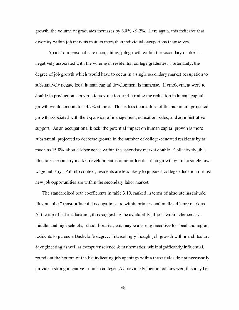
68

growth, the volume of graduates increases by 6.8% - 9.2%. Here again, this indicates that

diversity within job markets matters more than individual occupations themselves.

Apart from personal care occupations, job growth within the secondary market is

negatively associated with the volume of residential college graduates. Fortunately, the

degree of job growth which would have to occur in a single secondary market occupation to

substantively negate local human capital development is immense. If employment were to

double in production, construction/extraction, and farming the reduction in human capital

growth would amount to a 4.7% at most. This is less than a third of the maximum projected

growth associated with the expansion of management, education, sales, and administrative

support. As an occupational block, the potential impact on human capital growth is more

substantial, projected to decrease growth in the number of college-educated residents by as

much as 15.8%, should labor needs within the secondary market double. Collectively, this

illustrates secondary market development is more influential than growth within a single low-

wage industry. Put into context, residents are less likely to pursue a college education if most

new job opportunities are within the secondary labor market.

The standardized beta coefficients in table 3.10, ranked in terms of absolute magnitude,

illustrate the 7 most influential occupations are within primary and midlevel labor markets.

At the top of list is education, thus suggesting the availability of jobs within elementary,

middle, and high schools, school libraries, etc. maybe a strong incentive for local and region

residents to pursue a Bachelor’s degree. Interestingly though, job growth within architecture

& engineering as well as computer science & mathematics, while significantly influential,

round out the bottom of the list indicating job openings within these fields do not necessarily

provide a strong incentive to finish college. As previously mentioned however, this may be

69

due to the volume of laborers required in these fields relative to others. Also noteworthy is

the influence of job growth in farming relative to the primary and midlevel occupations with

lower standardized betas. In effect, county development within the farming industry may be

more of a deterrent to higher education than jobs with healthcare technology and computer

science are an incentive.

Discussion,ImplicationsforModelofIndividualsOverall, employment growth in several occupational categories was positively associated

with gains in counties’ high school graduate/G.E.D. stock, Associate’s degree earners, and

Bachelor’s degree earners. A comparative summary detailing the impact of job growth on

aggregate human capital is provided in table 3.11. Regarding the volume of county residents

with a high school degree or G.E.D., most growth was associated with increases in

employment increases within the midlevel labor market, specifically sales and administrative

support occupations. Job development within primary and secondary labor markets are also

positively associated with the volume of high school graduates, though surprising their

predicted slope effects are similar. Interestingly, job growth in two primary market

occupations is negatively associated with high school graduation. This is likely because jobs

within these industries require at least some form of postsecondary education. As such, job

growth in life, physical, and social sciences as well as architecture and engineering does not

incentive local residents to culminate their education with a high school degree nor does it

incentive high school graduates to relocate to counties with job opportunities in these fields.

Farming was the only secondary market occupation to negatively impact counties’ stock of

high school graduates. This suggests that a high school education is not necessary for farm

employment as the required skills needed for day-to-day tasks are learned on the job.

70

Growth in the remaining occupations, however, have a positive influence on the residential

stock of high school graduates, though to varying degrees.

Job growth in all labor market tiers and most occupations had a significant impact on

counties’ stock of Associate degree earners, with just six occupations proving uninfluential.

Three primary market occupations were positively associate with an increase in the number

of 2-year degree holders, specifically; healthcare, management, and education. Among mid-

market occupations, employment gains in protective services and installation & repair did not

significantly impact aggregate human capital growth, suggesting many jobs within these

sectors do not require education beyond high school, nor do they provide incentive to enroll

in college. As with high school graduation, the association between employment in farming

and Associate’s degree earners was also negative.

Comparatively, the influence of employment growth in primary and midlevel labor

markets on the volume of Associate degree earners is statistically identical, suggesting local

job opportunities in high-wage and medium-wage occupations incentivize college enrollment

equally. On the other hand, growth in secondary labor markets reduce growth of Associate’s

degree earners suggesting locals will not invest in a college degree if the job market does not

adequately compensate their efforts.

Nearly all primary market occupations influence growth in the number of college

educated residents, which is somewhat intuitive. Most occupations in fields like “Computers

& Mathematics,” “Architecture & Engineering,” etc. likely require a college degree as a

prerequisite for employment. Additionally, most midlevel occupations are positively

associate with the volume of Bachelor’s degree earners, though the influence of job growth

in the midlevel markets, as a whole, is slightly smaller. This is likely due to the varied

71

educational requirements of jobs nested within the subcategories of mid-market occupations.

Many jobs within sales and administrative support, for example, may require employees to

have an Associate’s or Bachelor’s degree before considering them for employment.

Only two mid-market occupations did not significantly contribute to counties’ stock of

Bachelor’s degree earners; specifically, protective service jobs and installation and repair

jobs. This suggests a large proportion of jobs within these industries do not require a college

education, hence employment growth within these occupations generally would not provide

incentive to pursue a postsecondary degree.

Lastly, four secondary market occupations were illustrated to impact the volume of

residential college graduates, three of which negatively so. While employment growth in

personal care has a small, positive influence on human capital growth, gains in production

and construction/extraction, and farming were negatively associated with human capital

growth. This suggests that most jobs grouped into these categories do not require their

employees to have earned a 4-year degree for employment, thus job opportunities in these

fields do not incentivize continuing one’s education beyond high school.

As illustrated, all labor market tiers and many individual occupations are associate with

local human capital growth via increases in the number of high school graduates, Associate’s

degree earners, and Bachelor’s degree earners. The caveat is that the extent of those gains is

dependent on the type of occupations available. Comparatively, expansion in primary

markets generated more growth than mid-level or secondary market occupations in terms of

4-year degree earners, yet did not increase the number of high school graduates as much as

mid-level markets. This pattern becomes more apparent when considering labor market tiers.

For example, counties’ stock of high school graduates was predicted to increase by 8.3% -

72

14.10% for each doubling of employment within primary market occupations, 29.3% - 36.0%

within mid-market occupations, and 9.0% - 15.2% within secondary market occupations. As

such, primary market job opportunities are about as influential as secondary job market

opportunities when it comes to growth in the number of high school graduates; midlevel

markets are far more influential in this respect.

The pattern between secondary market occupations and regional human capital growth is

also illustrative of a relationship between job type and educational credentials, with

associated gains in counties’ stock of Associate and Bachelor’s degree earners being

minimal—and in fact negative—compared to high school graduates/GED earners. At 100%

growth in the number of employed persons, in secondary markets are predicted to increase

the percent of high school graduates by 9.0% - 15.2%; decrease the volume of Associate’s

degree earners by 16.1% - 27.6%; and decrease the volume of Bachelor’s degree earners by

7.7% - 15.8%. These findings are in line with what human capital theory would predict;

growth in occupations which do not offer high wages, good benefits, etc. generates less

growth counties’ stock of high school graduates than college degree earners.

Overall, results indicate that growth in any job type, while somewhat influential to human

capital, does not make a substantial contribution. Sizable growth does not occur until

employment gains are several standard deviations above the mean. At this threshold, growth

in occupations like management, healthcare diagnostics, and education generate considerable

gains. As such, occupational gains are more influential as consolidated units, i.e., primary

market jobs (or tier 1), mid-level market jobs (tier 2) and secondary market jobs (tier 3). This

will be become more apparent when individual outcomes are regressed against employment

changes by occupation tiers.

73

HypothesesRevisited

Regarding hypotheses, results of the aggregate models are generally supportive. The

first hypothesis, “Local job markets with high employment growth in primary market

occupations—i.e., occupations which typically require education beyond high school—will

generate more high school graduates as well as Associate and Bachelor’s degree earners.”

received mixed support by the county-level models. Overall, Employment growth in primary

market occupations was positively associate with growth in each degree type, though the

volume of a growth varied by degree. Specifically, job growth in primary labor markets was

predicted to increase counties’ stocks of high school graduates by 8.3% - 14.1% per each

doubling of employment; increased Associate’s degree earners by 28.0% - 39.4%; and

Bachelor’s degree earners by 48.7% - 56.8%.

As for the second hypothesis, “growth in primary market occupations will generate a

larger increase in college degree earners, compared to the mid-level and secondary job

markets;” is partially supported. Specifically, expansion of primary market employment

increased counties’ stock of Bachelor’s degree earners yet midlevel market growth generated

more Associate’s degree earners.

Implicationsformodelofindividualoutcomes

Results from this chapter dictate which variables are used to assess the relationship

between county-level job growth and individuals’ educational attainment outcomes. Only

those occupations which have a significant impact on counties’ human capital growth are

included, thus job growth in “Architecture & Engineering,” “Production,” and

“Transportation” will not be used to assess the probability of graduating high school;

“Protective Services,” “Healthcare Support”, “Personal Care,” “Food Preparation,” and

74

“Maintenance” will not be used to assess earning a 2-year degree; etc. That said, a model

with all 23 ACS occupations grouped into their respective tiers will be utilized to evaluate

the aggregate influence of growth within primary, mid-level, and secondary markets. In

addition, results from this model will be used to support or refute hypotheses 3, 4, and 5.

Table 3.1. Summary Statistics

Variables Mean std. dev.

HS Degree/G.E.D. 0.207 0.166 Associate's Degree 0.417 0.271 Bachelor's Degree 0.351 0.281 Asian 0.604 1.159 Black 0.504 1.485 Hispanic 0.923 0.902 Native ‐0.095 0.550 Pacific 0.200 1.343 White ‐0.038 0.169 Two or more 0.434 0.850 Other ‐0.738 0.366 Rurality 0.050 0.027 Legal Occupations 0.211 0.684 Healthcare Practitioners 0.312 0.433 Life, Physical, and Social Sciences 0.134 0.676 Computers & Mathematics 0.446 0.876 Architecture & Engineering 0.077 0.585 Management 0.095 0.278 Business & Finance 0.191 0.433 Education, Training, & Libraries 0.097 0.306 Community & Social Services 0.207 0.521 Arts & Design, Entertainment 0.082 0.542 Healthcare Technologists 0.381 0.578 Protective Services 0.276 0.517 Sales 0.020 0.239 Office/Admin Support ‐0.016 0.191 Installation & Repair ‐0.093 0.277 Healthcare Support 0.269 0.484 Production ‐0.200 0.283 Transportation 0.028 0.273

75

Personal Care 0.291 0.434 Construction/Extraction ‐0.009 0.320 Food Preparation & Service 0.166 0.382 Maintenance Occupations 0.240 0.375 Farming 0.005 0.510 Primary Market Occupations 0.112 0.217 Mid‐Level Market Occupations ‐0.005 0.161 Secondary Market Occupations 0.022 0.188 N = 3,132

Table 3.2. Percent Change in the Number of Adults, 25 or older, with a High School Degree Model 1 Model 2 Model 3

B Std. Error B Std.

Error B Std. Error

Asian .012*** .003 .002 .002 .003 .002 Black 0.003 .003 ‐.006 .003 ‐.003 .003 Hispanic .023*** .005 .004 .004 ‐.001 .004 Native .001 .002 ‐.001 .002 .000 .002 Pacific .000 .002 ‐.003 .002 ‐.001 .002 White .133*** .013 .070*** .011 .068*** .011 Two or More ‐.008*** .004 ‐.013*** .003 ‐.013*** .003 Other ‐.024*** .001 ‐.003** .001 ‐.004** .001 Rurality ‐.013*** .008 ‐.004*** .001 ‐.002* .001 Primary Occupations .111*** .015 Mid‐Market Occupations .327*** .017

Secondary Occupations .123*** .015 Legal Occupations .002 .002 Healthcare Practitioners .007 .005 Life, Physical, and Social Sciences ‐.007** .002 Computers & Mathematics .002 .002 Architecture & Engineering ‐.006* .003 Management .075*** .010 Business & Finance ‐.009 .005 Education, Training, & Libraries .018* .008 Community & Social Services .000 .004 Arts & Design, Entertainment ‐.005 .003 Healthcare Technologists .007 .004 Protective Services .028*** .004 Sales .092*** .009 Office/Admin Support .142*** .012

76

Installation & Repair .030*** .007 Healthcare Support .030*** .005 Production .005 .006 Transportation .044*** .008 Personal Care .024*** .004 Construction/Extraction ‐.005 .007 Food Preparation & Service .042*** .007 Maintenance Occupations .020** .007 Farming ‐.011** .003 Constant .117*** .008 .087*** .008 .067*** .008 F 54.80 136.10 53.63

F‐Partial 328.28 46.01

R2 .134 .341 .350

*** = p< .001; ** = p < .01; * = p < .05

Table 3.3. Influence of Occupational Growth on Percent Change in Residential High School Graduates/G.E.D. Earners, 90% CI

Occupations Change per 1% increase

Change per 10% increase



Lower Upper Lower Upper Lower Upper Lower Upper Legal Occupations n.s. n.s. n.s. n.s. n.s. n.s. n.s. n.s. Healthcare Practitioners n.s. n.s. n.s. n.s. n.s. n.s. n.s. n.s. Life, Physical, and Social Sciences ‐0.01% 0.00% ‐0.11% ‐0.03% ‐0.55% ‐0.15% ‐1.10% ‐0.30% Computers & Mathematics n.s. n.s. n.s. n.s. n.s. n.s. n.s. n.s. Architecture & Engineering ‐0.01% 0.00% ‐0.11% ‐0.01% ‐0.55% ‐0.05% ‐1.10% ‐0.10% Management 0.06% 0.09% 0.57% 0.94% 2.85% 4.70% 5.70% 9.40% Business & Finance n.s. n.s. n.s. n.s. n.s. n.s. n.s. n.s. Education, Training, & Libraries 0.00% 0.03% 0.04% 0.32% 0.20% 1.60% 0.40% 3.20% Tier‐1 Occupations 0.09% 0.14% 0.87% 1.36% 4.35% 6.80% 8.70% 13.60% Community & Social Services n.s. n.s. n.s. n.s. n.s. n.s. n.s. n.s. Arts & Design, Entertainment ‐0.01% 0.00% ‐0.10% 0.00% ‐0.50% ‐0.01% ‐1.00% ‐0.01% Healthcare Technologists n.s. n.s. n.s. n.s. n.s. n.s. n.s. n.s. Protective Services 0.02% 0.04% 0.20% 0.37% 1.00% 1.85% 2.00% 3.70% Sales 0.08% 0.11% 0.76% 1.08% 3.80% 5.40% 7.60% 10.80% Office/Admin Support 0.12% 0.16% 1.23% 1.61% 6.15% 8.05% 12.30% 16.10% Installation & Repair 0.02% 0.04% 0.17% 0.40% 0.85% 2.00% 1.70% 4.00% Tier‐2 Occupations 0.30% 0.36% 2.98% 3.55% 14.90% 17.75% 29.80% 35.50% Healthcare Support 0.02% 0.04% 0.22% 0.40% 1.10% 2.00% 2.20% 4.00% Production n.s. n.s. n.s. n.s. n.s. n.s. n.s. n.s. Transportation 0.03% 0.06% 0.31% 0.60% 1.55% 3.00% 3.10% 6.00% Personal Care 0.02% 0.03% 0.15% 0.33% 0.75% 1.65% 1.50% 3.30%

77

Construction/Extraction n.s. n.s. n.s. n.s. n.s. n.s. n.s. n.s. Food Preparation & Service 0.03% 0.05% 0.30% 0.50% 1.50% 2.50% 3.00% 5.00% Maintenance Occupations 0.01% 0.03% 0.10% 0.30% 0.50% 1.50% 1.00% 3.00% Farming ‐0.02% ‐0.01% ‐0.20% ‐0.10% ‐1.00% ‐0.50% ‐2.00% ‐1.00% Tier‐3 Occupations 0.10% 0.15% 0.98% 1.47% 4.90% 7.35% 9.80% 14.70%

Table 3.4. Standardized Beta Coefficients, High School Graduation Std. Beta Office/Admin Support 0.192 Sales 0.155 Management 0.132 Food Preparation & Service 0.102 Healthcare Support 0.098 Protective Services 0.097 Transportation 0.086 Installation & Repair 0.069 Personal Care 0.069 Farming 0.048 Maintenance Occupations 0.046 Life, Physical, and Social Sciences 0.045 Education, Training, & Libraries 0.036 Architecture & Engineering 0.030

Table 3.5. Percent Change in the Number of Adults, 25 or older, with an Associate’s Degree Variables Model 1 Model 2 Model 3

B Std. Error B Std.

Error B Std. Error

Asian ‐.010* .005 ‐.019*** .004 ‐.020*** .004 Black .018** .006 .012 .006 .010 .006 Hispanic .022* .009 .000 .009 .000 .009 Native ‐.008 .005 ‐.006 .004 ‐.007 .004 Pacific ‐.001 .003 ‐.002 .003 ‐.002 .003 White .258*** .023 .146*** .022 .162*** .022 Two or More ‐.001 .007 .005 .006 .003 .006 Other ‐.010*** .003 ‐.006* .002 ‐.005* .002 Rurality ‐.001 .002 ‐.010*** .002 .010*** .002 Primary Occupations (Tier‐1) .337*** .029 Mid‐Market Occupations (Tier‐2) .405*** .034

78

Secondary Occupations (Tier‐3) ‐.218*** .029 Legal Occupations .008 .004 Healthcare Practitioners .089*** .011 Life, Physical, and Social Sciences ‐.004 .004 Computers & Mathematics .006 .005 Architecture & Engineering .000 .006 Management .075*** .019 Business & Finance .005 .009 Education, Training, & Libraries .076*** .017 Community & Social Services .031*** .008 Arts & Design, Entertainment ‐.017** .006 Healthcare Technologists .023** .008 Protective Services .001 .009 Sales .099*** .018 Office/Admin Support .188*** .023 Installation & Repair .024 .013 Healthcare Support ‐.005 .009 Production ‐.028* .013 Transportation ‐.036* .016 Personal Care .017 .011 Construction/Extraction ‐.003 .014 Food Preparation & Service ‐.004 .013 Maintenance Occupations ‐.002 .014 Farming ‐.030*** .007 Constant .413*** .015 .350*** .015 .345*** .016 F 22.61 52.80 20.12

Partial F ‐‐ 134.68 18.02

R2 .059 .166 .164

*** = p< .001; ** = p < .01; * = p < .05; ~ = p < .01

Table 3.6. Influence of Occupational Growth on Percent Change in Residential Associate’s Degree Earners, 90% CI





Lower Upper Lower Upper Lower Upper Lower Upper Legal Occupations 0.00% 0.02% 0.04% 0.15% 0.20% 0.75% 0.40% 1.50%Healthcare Practitioners 0.07% 0.11% 0.70% 1.10% 3.50% 5.50% 7.00% 11.00%Life, Physical, and Social Sciences n.s. n.s. n.s. n.s. n.s. n.s. n.s. n.s. Computers & Mathematics n.s. n.s. n.s. n.s. n.s. n.s. n.s. n.s. Architecture & Engineering n.s. n.s. n.s. n.s. n.s. n.s. n.s. n.s. Management 0.04% 0.11% 0.37% 1.11% 1.85% 5.55% 3.70% 11.10%

79

Business & Finance n.s. n.s. n.s. n.s. n.s. n.s. n.s. n.s. Education, Training, & Libraries 0.05% 0.10% 0.48% 1.03% 2.40% 5.15% 4.80% 10.30%Tier‐1 Occupations 0.27% 0.36% 2.72% 3.64% 13.60% 18.20% 27.20% 36.40% Community & Social Services 0.02% 0.04% 0.17% 0.44% 0.85% 2.20% 1.70% 4.40%Arts & Design, Entertainment ‐0.03% ‐0.01% ‐0.28% ‐0.05% ‐1.39% ‐0.25% ‐2.77% ‐0.50%Healthcare Technologists 0.01% 0.04% 0.07% 0.39% 0.35% 1.94% 0.70% 3.87%Protective Services n.s. n.s. n.s. n.s. n.s. n.s. n.s. n.s. Sales 0.07% 0.13% 0.68% 1.29% 3.40% 6.45% 6.80% 12.90%Office/Admin Support 0.15% 0.23% 1.49% 2.27% 7.45% 11.35% 14.90% 22.70%Installation & Repair 0.00% 0.05% 0.02% 0.46% 0.10% 2.30% 0.20% 4.60%Tier‐2 Occupations 0.36% 0.47% 3.64% 4.73% 18.20% 23.65% 36.40% 47.30% Healthcare Support n.s. n.s. n.s. n.s. n.s. n.s. n.s. n.s. Production ‐0.05% ‐0.01% ‐0.52% ‐0.06% ‐2.60% ‐0.30% ‐5.20% ‐0.60% Transportation ‐0.06% ‐0.01% ‐0.62% ‐0.06% ‐3.10% ‐0.30% ‐6.20% ‐0.60% Personal Care n.s. n.s. n.s. n.s. n.s. n.s. n.s. n.s. Construction/Extraction n.s. n.s. n.s. n.s. n.s. n.s. n.s. n.s. Food Preparation & Service n.s. n.s. n.s. n.s. n.s. n.s. n.s. n.s. Maintenance Occupations n.s. n.s. n.s. n.s. n.s. n.s. n.s. n.s. Farming ‐0.04% ‐0.02% ‐0.40% ‐0.18% ‐2.00% ‐0.90% ‐4.00% ‐1.80%Tier‐3 Occupations ‐0.28% ‐0.16% ‐2.76% ‐1.61% ‐13.78% ‐8.07% ‐27.55% ‐16.13%

Table 3.7. Standardized Beta Coefficients, Associate Degree Attainment Occupations Std. Beta Healthcare Practitioners 0.151Office/Admin Support 0.146Sales 0.096Education, Training, & Libraries 0.088Management 0.075Farming ‐0.074Community & Social Services 0.065Healthcare Technologists 0.050Arts & Design, Entertainment 0.050Transportation ‐0.040Production ‐0.039Installation & Repair 0.032Legal Occupations 0.029

80

Table 3.8. Percent Change in the Number of Adults, 25 or older, with an Associate’s Degree Variables Model 1 Model 2 Model 3

B Std. Error B Std.

Error B Std. Error

Asian .019*** .004 .005 .003 .004 .003 Black .021*** .005 .012** .004 .012** .004 Hispanic .042*** .007 .009 .006 .004 .006 Native ‐.004 .004 ‐.004 .003 ‐.005 .003 Pacific .003 .002 .001 .002 .002 .002 White .227*** .018 .078*** .016 .093*** .016 Two or More ‐.012* .005 ‐.001 .004 ‐.005 .002 Other ‐.009*** .002 ‐.003 .002 ‐.003 .005 Rurality ‐.017*** .001 ‐.002 .001 .001 .001 Primary Occupations (Tier‐1) .508*** .020 Mid‐Market Occupations (Tier‐2) .338*** .024

Secondary Occupations (Tier‐3) ‐.113*** .021 Legal Occupations .004 .003 Healthcare Practitioners .049*** .008 Life, Physical, and Social Sciences .002 .003 Computers & Mathematics .007* .003 Architecture & Engineering .009* .004 Management .144*** .014 Business & Finance .045*** .007 Education, Training, & Libraries .176*** .012 Community & Social Services .032*** .006 Arts & Design, Entertainment .011** .004 Healthcare Technologists .018** .006 Protective Services .009 .006 Sales .122*** .013 Office/Admin Support .113*** .017 Installation & Repair .004 .010 Healthcare Support ‐.005 .007 Production ‐.027** .009 Transportation .004 .012 Personal Care .024** .008 Construction/Extraction ‐.028** .010 Food Preparation & Service .002 .009 Maintenance Occupations .003 .010 Farming ‐.019*** .005 Constant .314*** .011 .209*** .011 .210*** .012 F 72.34 178.23 64.81

Partial F ‐‐ 410.45 51.31

81

R2 .170 .405 .394

*** = p< .001; ** = p < .01; * = p < .05

Table 3.9. Influence of Occupational Growth on Percent Change in Residential Bachelor’s Degree Earners, 90% CI





Lower Upper Lower Upper Lower Upper Lower Upper Legal Occupations n.s. n.s. n.s. n.s. n.s. n.s. n.s. n.s. Healthcare Practitioners 0.04% 0.06% 0.36% 0.61% 1.80% 3.05% 3.60% 6.10% Life, Physical, and Social Sciences n.s. n.s. n.s. n.s. n.s. n.s. n.s. n.s. Computers & Mathematics 0.00% 0.01% 0.01% 0.12% 0.05% 0.60% 0.10% 1.20% Architecture & Engineering 0.00% 0.02% 0.02% 0.16% 0.10% 0.80% 0.20% 1.59% Management 0.12% 0.17% 1.21% 1.66% 6.05% 8.30% 12.10% 16.60% Business & Finance 0.03% 0.06% 0.34% 0.55% 1.70% 2.75% 3.40% 5.50% Education, Training, & Libraries 0.16% 0.20% 1.56% 1.95% 7.80% 9.75% 15.60% 19.50% Primary Market Occupations 0.48% 0.54% 4.76% 5.41% 23.80% 27.05% 47.60% 54.10% Community & Social Services 0.02% 0.04% 0.22% 0.42% 1.10% 2.10% 2.20% 4.19% Arts & Design, Entertainment 0.00% 0.02% 0.04% 0.18% 0.20% 0.89% 0.40% 1.77% Healthcare Technologists 0.01% 0.03% 0.08% 0.28% 0.40% 1.38% 0.80% 2.75% Protective Services n.s. n.s. n.s. n.s. n.s. n.s. n.s. n.s. Sales 0.10% 0.14% 0.96% 1.43% 4.80% 7.15% 9.60% 14.30% Office/Admin Support 0.09% 0.14% 0.85% 1.40% 4.25% 7.02% 8.50% 14.04% Installation & Repair n.s. n.s. n.s. n.s. n.s. n.s. n.s. n.s. Midlevel Market Occupations 0.30% 0.37% 2.99% 3.75% 14.95% 18.73% 29.90% 37.45% Healthcare Support n.s. n.s. n.s. n.s. n.s. n.s. n.s. n.s. Production ‐0.04% ‐0.01% ‐0.41% ‐0.12% ‐2.07% ‐0.59% ‐4.13% ‐1.18% Transportation n.s. n.s. n.s. n.s. n.s. n.s. n.s. n.s. Personal Care 0.01% 0.04% 0.12% 0.37% 0.59% 1.84% 1.18% 3.67% Construction/Extraction ‐0.04% ‐0.01% ‐0.44% ‐0.11% ‐2.20% ‐0.55% ‐4.40% ‐1.09% Food Preparation & Service n.s. n.s. n.s. n.s. n.s. n.s. n.s. n.s. Maintenance Occupations n.s. n.s. n.s. n.s. n.s. n.s. n.s. n.s. Farming ‐0.03% ‐0.01% ‐0.27% ‐0.11% ‐1.35% ‐0.57% ‐2.70% ‐1.15% Secondary Market Occupations ‐0.15% ‐0.08% ‐1.47% ‐0.79% ‐7.35% ‐3.95% ‐14.69% ‐7.90%

82

Table 3.10. Standardized Beta Coefficients, Bachelor’s Degree Attainment Std. Beta Education, Training, & Libraries 0.243 Management 0.172 Sales 0.140 Office/Admin Support 0.104 Business & Finance 0.101 Healthcare Practitioners 0.097 Community & Social Services 0.081 Farming ‐0.058 Personal Care 0.048 Healthcare Technologists 0.046 Production ‐0.044 Construction/Extraction ‐0.041 Arts & Design, Entertainment 0.039 Architecture & Engineering 0.032 Computers & Mathematics 0.028

83

Table 3.11. Influence of Occupational Growth on Percent Change in Human Capital Development, 90% CI

Volume of High School Degrees Volume of Associate’s Degrees Volume of Bachelor's Degrees







Lower 95% CI

Upper 95% CI

Lower 95% CI

Upper 95% CI

Lower 95% CI

Upper 95% CI

Lower 95% CI

Upper 95% CI

Lower 95% CI

Upper 95% CI

Lower 95% CI

Upper 95% CI

Legal Occupations n.s. n.s. n.s. n.s. 0.20% 0.75% 0.40% 1.50% n.s. n.s. n.s. n.s. Healthcare Practitioners n.s. n.s. n.s. n.s. 3.50% 5.50% 7.00% 11.00% 1.80% 3.05% 3.60% 6.10% Life, Physical, and Social Sciences ‐0.55% ‐0.15% ‐1.10% ‐0.30% n.s. n.s. n.s. n.s. n.s. n.s. n.s. n.s. Computers & Mathematics n.s. n.s. n.s. n.s. n.s. n.s. n.s. n.s. 0.05% 0.60% 0.10% 1.20% Architecture & Engineering ‐0.55% ‐0.05% ‐1.10% ‐0.10% n.s. n.s. n.s. n.s. 0.10% 0.80% 0.20% 1.59% Management 2.85% 4.70% 5.70% 9.40% 1.85% 5.55% 3.70% 11.10% 6.05% 8.30% 12.10% 16.60% Business & Finance ‐1.00% ‐5.00% ‐2.00% ‐10.00% n.s. n.s. n.s. n.s. 1.70% 2.75% 3.40% 5.50% Education, Training, & Libraries 0.20% 1.60% 0.40% 3.20% 2.40% 5.15% 4.80% 10.30% 7.80% 9.75% 15.60% 19.50% Tier‐1 Occupations 4.35% 6.80% 8.70% 13.60% 14.00% 19.70% 28.00% 39.40% 24.68% 28.08% 49.36% 56.15% Community & Social Services n.s. n.s. n.s. n.s. 0.85% 2.20% 1.70% 4.40% 1.10% 2.10% 2.20% 4.19% Arts & Design, Entertainment ‐0.50% ‐0.01% ‐1.00% ‐0.01% ‐1.39% ‐0.25% ‐2.77% ‐0.50% 0.20% 0.89% 0.40% 1.77% Healthcare Technologists n.s. n.s. n.s. n.s. 0.35% 1.94% 0.70% 3.87% 0.40% 1.38% 0.80% 2.75% Protective Services 1.00% 1.85% 2.00% 3.70% n.s. n.s. n.s. n.s. n.s. n.s. n.s. n.s. Sales 3.80% 5.40% 7.60% 10.80% 3.40% 6.45% 6.80% 12.90% 4.80% 7.15% 9.60% 14.30% Office/Admin Support 6.15% 8.05% 12.30% 16.10% 7.45% 11.35% 14.90% 22.70% 4.25% 7.02% 8.50% 14.04% Installation & Repair 0.85% 2.00% 1.70% 4.00% 0.10% 2.30% 0.20% 4.60% n.s. n.s. n.s. n.s. Tier‐2 Occupations 14.90% 17.75% 29.80% 35.50% 16.95% 23.50% 33.90% 47.00% 10.01% 17.93% 20.01% 35.85% Healthcare Support 1.10% 2.00% 2.20% 4.00% n.s. n.s. n.s. n.s. n.s. n.s. n.s. n.s. Production n.s. n.s. n.s. n.s. ‐2.60% ‐0.30% ‐5.20% ‐0.60% ‐2.07% ‐0.59% ‐4.13% ‐1.18% Transportation 1.55% 3.00% 3.10% 6.00% ‐3.10% ‐0.30% ‐6.20% ‐0.60% n.s. n.s. n.s. n.s. Personal Care 0.75% 1.65% 1.50% 3.30% n.s. n.s. n.s. n.s. 0.59% 1.84% 1.18% 3.67% Construction/Extraction n.s. n.s. n.s. n.s. n.s. n.s. n.s. n.s. ‐2.20% ‐0.55% ‐4.40% ‐1.09% Food Preparation & Service 1.50% 2.50% 3.00% 5.00% n.s. n.s. n.s. n.s. n.s. n.s. n.s. n.s. Maintenance Occupations 0.50% 1.50% 1.00% 3.00% n.s. n.s. n.s. n.s. n.s. n.s. n.s. n.s. Farming ‐1.00% ‐0.50% ‐2.00% ‐1.00% ‐2.00% ‐0.90% ‐4.00% ‐1.80% ‐1.35% ‐0.57% ‐2.70% ‐1.15% Tier‐3 Occupations 4.90% 7.35% 9.80% 14.70% ‐13.78% ‐8.07% ‐27.55% ‐16.13% ‐7.58% ‐3.84% ‐15.15% ‐7.69%

84

CHAPTERIV

THEINFLUENCEOFEMPLOYMENTGAINSINPRIMARY

MARKETSONTHEPROBABILITYOFGRADUATINGHIGH

SCHOOLAND/OREARNINGACOLLEGEDEGREE

This chapter tests hypotheses 3, 4, and 5; evaluating the influence of employment growth

within primary, midlevel, and secondary labor markets on the probability of graduating high

school, earning an Associate’s degree, and earning a Bachelor’s degree. In addition, the

influence of job growth in individual occupations within each labor market tier is assessed.

Results indicate employment growth plays a small yet significant role in respondents’

education outcomes. Networks, however, play a much larger role.

DescriptiveStatisticsofIndividualOutcomes

Table 4.1 details the summary statistics for variables used in logistic models. Overall,

95.5% of participants completed high school or earned a G.E.D., suggesting a sampling bias

within the data. According to the most recent ACS 5-year estimate, 86.3% of the US

population have earned a high school degree or its equivalent—nearly 10% less the than

graduation rate of ELS respondents. Here, self-selection bias is the most likely cause of the

skew. Respondents who participated in the ELS survey may value education more than the

general public.

In regards to demographics, the sample is reflective of the general population in some

aspects but differs in others. Males and females have roughly equal representation with 50%

of each included in the sample. Asians constitute 9.7% of respondents, though in 2000 and

85

2005, roughly the timeframe when potential respondents were contacted, Asians accounted

for just 3.5% and 4.3% of the population, respectively. Population figures for Blacks,

Hispanics, and Native Americans (accounting for 12%, 13%, and 1% of the sample

respectively) are moreorless in line with those from the 2000 census and 2005 ACS, plus or

minus 1%. Parent’s income also suggests a slight upward skew within the sample data, as the

average US household income in 2000—just two years prior to the first wave of survey

interviews—hovered around $55,000. The average income of respondents’ parents is just

above $69,000. As for parents’ highest level of education, most had at least some college

experience, but did not necessarily obtain a 2-year or 4-year degree (an average of 13.46

years of education).

As illustrated in table 4.1, the average number of respondents’ friends who planned to

attend community college after high school falls between “Some” and “Most.”

Comparatively, respondents reported that “Most” to “All” of their friends had plans to attend

a 4-year college. It’s difficult to ascertain how representative these figures are of the general

populous circa 2004, the year most ELS participants would have graduated. According to the

National Center for Higher Education Management Systems (NCHEMS)23, 55.7% of

graduates enrolled in college the following semester (in 2004). This would roughly

correspond to “Most.”

On average, respondents reported about two-thirds of persons with whom they have close

ties encouraged them to enroll in college. Here again, the purpose of this measure is to gauge

the degree to which respondents feel they are expected to pursue a college degree; the more

encouraged they feel to continue their education beyond high school, the more likely they

23 http://www.higheredinfo.org/dbrowser/?year=2004&level=nation&mode=map&state=0&submeasure=63

86

will actually graduate high school. The average of this index variable suggests that over half

of respondents’ close ties wanted them to continue their education. In comparison, very few

respondents reported their close ties preferred them to get a job instead of pursuing a

postsecondary degree. In fact, of the 12,670 respondents, less than 10% believed any of their

ties wanted them to seek employment immediately after graduation. Corollary, and at the

school level, an average of 44.5% of the previous year’s graduating class enrolled at 4-year

universities the following semester, and 11.33% entered the job market.

By and large, most respondents attended high school in metro counties with a population

nearing 250,000, as suggested by an average rurality score of 2.95. Regarding primary

market occupations, there was growth among all job types, from a low of 1.23% in

architecture and engineering to a maximum of 36.39% in healthcare practitioner jobs.

Compared to the descriptive statistics for the aggregate model (table 3.1), employment gains

in the logistic model differ substantially, likely due to the smaller number of counties

included in the model as well as repeated observations. For example, average employment

gains in management and education, educational training, and library occupations were

9.46% and 9.71%, respectively, when all 3,142 counties are included. When the sample is

reduced to 710—the number of counties corresponding to respondents’ high school

locations—employment gains increase to 18.14% and 19.74% respectively. In addition, the

spread in employment growth by occupation is not as pronounced. This suggests that

respondents’ counties of origin may fundamentally differ from counties not included in the

logistic model. Overall, job growth in primary labor markets averaged 22.2%.

From 2000 to 2014, there was 4.2% employment gain in mid-level market occupations,

with a large degree of variation by job type. For example, employment in installation &

87

repair as well as office and administrative support positions decreased by 8.4% and 2.4%,

respectively. At the other extreme, employment in healthcare technologies, protective

services, and community & social services increased by an average of 41.7%, 28.2%, and

26.2%, respectively. There were modest expansions within art, design, & entertainment as

well as sales occupations, each experiencing 11.6% and 6.3% growth.

Average county growth in the majority of secondary market occupations was substantial,

with the only decline occurring in production. Positive growth in both healthcare support and

personal care, coupled with employment gains in healthcare technologies and healthcare

diagnoses suggest a general upward trend in demand for health-related occupations; a pattern

most likely attributable to an aging baby-boom population, many of which are approaching

retirement. Average employment growth in maintenance as well as food preparation and

service jobs was considerably larger compared to growth in the majority of occupations in all

three tiers. This suggests a continued increase in service based occupations.

Comparing average employment gains within each occupational tier, there was more

growth within primary labor markets at 22.2%. Additionally, growth within each individual

tier-1 occupation exceeds 15%, and three exceed 20%. This suggests an increasing demand

for skilled workers among employers, which is hypothesized to have a positive impact on the

likelihood of graduating high school, earning an Associate’s degree, and earning a Bachelor’s

degree. Job growth within the mid-level market was substantially smaller at just 4.2%

between 2000 and 2014. Growth within the secondary market was more than three times that

of mid-market occupations at 13.8%.

88

LogisticModelResults

HighSchoolGraduation/G.E.D.Table 4.2 highlights the odds of earning a high school degree or a G.E.D. based on

assessed independent variables across three models. Model 1 details the influence of rurality

and information access about college via network/homophily effects. Model 2 introduces

employment growth within primary, midlevel, and secondary labor markets. The final model

accounts for all three tiers, rurality, and network/homophily effects. Of note, the influence of

control variables is not displayed in any of the models.

Indicated in model 1, networks/homophily have a significant impact on the probability of

graduating high school. Respondents who reported their friends planned on attending college

were more likely to graduate compared to their counterparts. Here, the magnitude and

significance is dependent on the type of college respondents’ friends want to attend.

Participants were projected to be 10.2% more likely to graduate high school if some of their

friends planned to attend a 2-year community college and 51.2% more likely if they planned

to enroll at a 4-year university. Corollary, those who reported nearly all of their friends

planned to attend a 2-year or 4-year college are projected to be 30.6% and 153.3% more

likely to graduate.

Students believing their family, friends, peers, etc. wanted them to enroll in college were

more likely to graduate high school. Respondents who reported that at least one close family

member, peer, or school faculty member encouraged them to attend college were nearly

30%24 more likely to graduate or earn a G.E.D. This suggests the average student would

more than likely graduate, since participants reported receiving encouragement from about 3

24 Percentages will no longer be referred to as projections, though it should still be assumed.

89

close ties. High school graduation was not effected by encouragement to enter the job

market though. This is likely due to most occupations requiring potential employees to have

at least earned a high school degree.

The percentage of the previous year’s graduating class that enrolled in college or entered

the job market had a positive effect on the likelihood of graduation. In both instances,

respondents were 2.4% more likely to graduate for each percentage increase in the number of

the previous year’s cohort that went to a 4-year university. The location of respondents’ high

schools also influenced whether they graduated, with rural schools outperforming urban and

suburban schools.

The constant for model 1 indicates that, on average, students have a fairly high likelihood

of finishing high school—predicted to be about 80%. Regarding fit, two test statistics will be

utilized to gauge whether the addition of labor market and occupation variables improve the

base model. The BIC is used to determine if the inclusion of additional variables offers more

explanatory power, controlling for the number of factors used. Ideally, the BIC value should

decrease the more complex the model becomes, indicating a better fit. Tjur’s-R2 will be used

in conjunction with the BIC, though it is not based on the percent reduction of the negative

log likelihood. Instead, it is the difference between the predicted mean likelihood of an event

occurring and the predicted mean likelihood of the event not occurring. In model 1, for

example, the predicted mean likelihood of respondents graduating high school was 95.5%

while the predicted mean of not graduating was 4.5%. The difference between the two

values is 91%.25 Whereas the BIC should ideally decrease with the addition of occupational

variables, the Tjur’s R2 should increase, indicating the gap between the predicted mean of

25 For a more in depth discussion of Tjur’s R2, see Tjur (2009).

90

graduating, earning a Associate’s etc. and the predicted mean of not graduating, etc. has

widened.

In model 2, the influence of employment growth within primary, midlevel, and secondary

labor markets are added to the model. Whereas the influence of job growth in individual

occupations may be too small to measure, collapsing occupations into their respective tiers

may illuminate labor market influences on high school graduation that are otherwise

invisible. Results indicate that employment gains within primary labor markets are a

significant predictor of finishing high school/earning a G.E.D. Here, a 1% increase in

employment is predicted to generate a 2.37% increase in the likelihood of graduating.

Attending high school in counties where primary market job growth was extreme would

heavily influence respondents’ educational outcomes. If primary market employment were

to increase by 10%, respondents are predicted to be 23.7% more likely to graduate; at 25% it

increases to 59.3%, and so on. In short, employment growth in high-skill, high-wage

occupations begets an increased likelihood of finishing high school, thus it may function as

an incentive for students to invest in their education. Regarding model fit though, the Tjur’s

R2 (still .911), BIC (increased from 3253.03 to 3276.62), and network/homophily factors are

virtually unchanged compared to model 1. This suggests the inclusion of job growth by

occupational tier does not add any additional explanatory power to the base model, despite

the significance of growth within primary markets.

Model 3 parses out occupations within each labor market tier which were found to

significantly affect local human capital growth. As with models 1 and 2, respondents who

attended high school in rural and suburban counties were more likely graduate, all other

factors being equal. Additionally, the predicted magnitude of effect was roughly the same as

91

in previous models, or about a 12.8% increased/decreased chance of graduating per unit

change. Among primary market occupations, employment growth within management and

business & finance are illustrated to increase the odds of obtaining a degree. Regarding

management, the impact is substantial, predicted to increase the likelihood of graduation by

1.9% for every 1% increase in employment. This suggests the availability of jobs within

management may incentivize students to finish high school as they may not be considered for

these positions otherwise. On the other hand, it may reflect resources made available to local

schools. Given management occupations are classified as high-wage, an increase in the

number of persons employed in these positions would likely constitute an increase in local

school revenues via property taxes. Though job development in business & finance does not

seem as influential given its slope effect, the influence is still noteworthy, projected to

increase the odds of graduation by an average of .553% per percent employment growth. In

addition, the standard error for growth in management indicates its effect size could be

markedly lower than what is reported in model 3.

Regarding midlevel and secondary market occupations, none of the former are

significantly influential. Among secondary market occupations, employment growth in food

preparation & service negatively impact on graduation; predicted to decrease the likelihood

by .621% per 1% increase in employment. Here, this may indicate respondents are less

motivated to finish high school if local job opportunities do not require it. As with

management, however, it could also reflect local school funding—food service occupations

are low-wage, hence funds available to local schools would likely decrease within counties

where development of the food and service industry was rapid and extreme.

92

As for model fit, the Tjur’s R2 remains unchanged when all occupational factors are

incorporated into the model. Additionally, the BIC increases from 3253.03 in the base model

to 3366.29 in the full model. This suggests that county-level predictors did not add any

additional explanatory power to the networks/homophily model despite the influence of

employment gains in primary labor markets, management occupations, and the food and

service industry. As with models 1 and 2, network/homophily factors are virtually

unchanged.

Summary:Networks/Homophily,EmploymentGrowth,andHighSchoolGraduation

Table 4.3 summarizes influential factors of high school graduation as well as a few non-

significant factors for added context. Broken up into four sections, the table converts odds

ratios to percentages and details how a unit change in “x” affects “y”. The unit of change is

unique in each section, thus each has its own designated heading. Here, the purpose is to

better compare and contrast the roles of social networks/homophily and job growth on

earning a high school degree/G.E.D.

Overall, networks/homophily are more influential on respondents’ educational outcomes

compared to local job growth. Regarding “Networks & Homophily 1,” students who

reported at least a few of their friends had college aspirations were more likely to finish high

school. If most of their friends planned to attend college, the likelihood of graduation was

amplified. It is important to note, however, the extreme range associated with each network

factor. For example, if a few friends planned to attend community college, respondents are

projected to be 2.2% - 18.4% more likely to finish high school. If most of their friends

planned to attend community college the range increases to 6.6% - 55.2%. Another way of

interpreting this is having connections to people with minor college ambition may influence

93

one’s education a little or a lot. What can be said with more certainty is the difference of

influence between having friends who want to go to community college vs. having friends

who want to go to a 4-year college is substantial. Having just a few Bachelor’s-seeking

friends is projected to increase the likelihood of graduation by 41.1% - 63.4%.

The expectations of others also exert a substantial influence as to whether respondents

finished high school or earned a G.E.D. Having at least one contact who harbors college

aspirations for the respondent is projected to increase their odds of graduating by 24.2% -

35.5%. The strongest network/homophily predictors, however, were the actions of the

previous graduating cohort. For example, if students were enrolled at an institute in which

25% of the previous cohort attended a 4-year college; they were 50.0% - 72.5% more likely

to graduate. If 25% of the previous cohort entered the job market, respondents were 42.5% -

87.5% more likely to graduate.

Job growth within counties can substantially impact the odds of finishing high school.

As with a few networks/homophily effects, however, there is some uncertainty as to just how

impactful it actually is. For example, employment growth within management was predicted

to have a positive influence on the odds of high school graduation. From table 4.3, the

projected likelihood of graduating increases by .39% - 4.9% for each 1% increase in

employment. Of the 710 counties included in this analysis, the volume of persons employed

in management increased by 100% or more in 4 of them. So, in those four counties the

likelihood of finishing high school is projected to have increased by at least 39.0% - 490.0%.

Similarly, employment growth within primary markets is projected to increase the likelihood

of high school graduation by .33% - 7.52% per 1% increase. Within the same four counties,

growth in primary market employment also exceeded 100%, equating to an increased

94

likelihood of 33.0% - 752.0%. Collectively, this indicates very few counties experienced

extreme growth in the number of management and/or primary market positions, and among

those that did, the impact could have ranged from extreme to minimal. As such, all that can

be said is that perceived job opportunities within management and/or primary market

occupations potentially incentivizes students to finish high school.

Associate’sDegree

Table 4.4 details the log-odds results of obtaining an Associate’s degree based on

employment growth within county labor markets and network/homophily effects. Several

network/homophily measures significantly influence the odds of earning a junior college

degree. First, respondents were more likely to earn an Associate’s if at least some of their

friends planned to attend a 2-year college after high school and less likely if they planned to

attend a 4-year college. Regarding the former, students were predicted to be 26.1% more

likely to obtain a degree if at least some their friends planned to attend community college.

If all of their friends planned to enroll, this figure increases to 78.3%. As for the latter,

respondents were 12.1% less likely to earn a 2-year degree if some of their friends planned to

attend a 4-year university and 36.3% less likely if all of them planned to enroll.

Whether respondents believed they were expected to go to college and/or enter the labor

market after high school is also illustrated to affect their educational outcomes. Those who

felt their parents, friends, peers, etc. wanted them to go to college were more likely to

continue their education and earn an Associate’s. Those who felt expected to enter the job

market were less likely to earn a degree, though it is unclear whether this means they were

also less likely to pursue a postsecondary degree, and/or more likely to get a job immediately

after high school.

95

Respondents who felt that at least one of their close ties (mother, father, other relative,

friend, school counselor, etc.) wanted them to enroll in college were projected to be 5.8%

more likely to do so, eventually earning a degree. If all measured ties encouraged them to

continue, the predicted odds increased to 34%. Comparatively, believing friends and relatives

prefer labor market entry to college enrollment is a stronger incentive; on average,

respondents were projected to be 15.3% less likely to earn a 2-year degree for each tie they

believed would prefer it if they [respondents] would get a job after graduation. If

respondents believed this of all measured ties, it is projected to decrease the odds by 91.8%.

From model 2, employment growth in primary and secondary labor markets significantly

impact the likelihood of earning an Associate’s. Regarding primary labor markets, job

growth positively influences on education outcomes predicted to increase the odds of earning

a degree by about 1.5% for each 1% increase in employment. Growth within secondary

markets has the opposite effect, reducing the likelihood of degree obtainment by about .56%

per 1% gain in employment. Mid-level market occupations do not influence degree

attainment. Taken together, this supports the assumption that access to higher paying and

higher skilled jobs increases the likelihood of local residents investing in their education.

Likewise, respondents are less likely to pursue education beyond high school if it is not

requirement for local employment.

Regarding fit, a slightly larger BIC statistic for model 2 indicates the addition of labor

market effects to network/homophily factors does not add additional explanatory power to

the model despite the significant influence of primary and secondary market growth. In

addition, the Tjur’s R2 remains static at .87. This suggests that while occupational

96

opportunities may incentivize respondents to pursue a 2-year degree, the educational

preferences of persons within their networks is more influential.

In the full model, employment growth in four occupations significantly impacts

respondents’ educational outcomes. Within the primary market, growth in the healthcare

industry increases the likelihood of earning an Associate’s; suggesting local development

within the medical field may incentivize students to pursue a postsecondary education.

Within local midlevel labor markets, job creation within art, design, and entertainment is

negatively influential, predicted to reduce the likelihood of degree attainment by an average

of .28% per 1% of employment growth. This suggests students are less likely to consider a

career in the entertainment industry when deciding whether they should enroll in college.

Further, this likely indicates students believe a high school education is sufficient enough for

most entertainment-related occupations.

Among secondary market occupations, an increased availability of production and

farming jobs reduces the likelihood of earning an Associate. Employment growth within

production, for example, is predicted to decrease the odds by an average of about .4% per 1%

increase in persons employed within the industry. Further development of the farming

industry decreases the odds by about .133% per percent growth. Taken together, this

suggests job development within local secondary labor markets does not incentivize students

to pursue a postsecondary education. Instead, it suggests students are more likely to enter the

labor market after high school graduation as local job opportunities do not require additional

schooling.

As for fit, the full model does not increase Tjur’s R2 yet the associated BIC increases by

nearly 80 compared to the base model. As such, the inclusion of occupational variables does

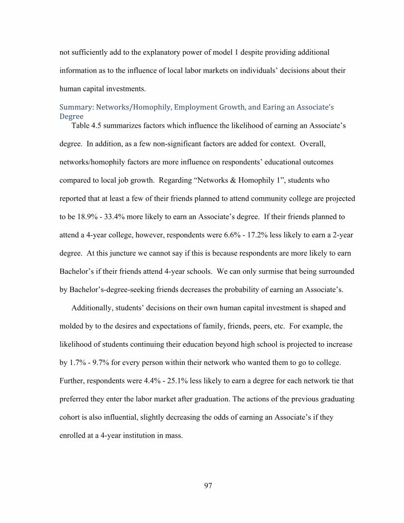
97

not sufficiently add to the explanatory power of model 1 despite providing additional

information as to the influence of local labor markets on individuals’ decisions about their

human capital investments.

Summary:Networks/Homophily,EmploymentGrowth,andEaringanAssociate’sDegree

Table 4.5 summarizes factors which influence the likelihood of earning an Associate’s

degree. In addition, as a few non-significant factors are added for context. Overall,

networks/homophily factors are more influence on respondents’ educational outcomes

compared to local job growth. Regarding “Networks & Homophily 1”, students who

reported that at least a few of their friends planned to attend community college are projected

to be 18.9% - 33.4% more likely to earn an Associate’s degree. If their friends planned to

attend a 4-year college, however, respondents were 6.6% - 17.2% less likely to earn a 2-year

degree. At this juncture we cannot say if this is because respondents are more likely to earn

Bachelor’s if their friends attend 4-year schools. We can only surmise that being surrounded

by Bachelor’s-degree-seeking friends decreases the probability of earning an Associate’s.

Additionally, students’ decisions on their own human capital investment is shaped and

molded by to the desires and expectations of family, friends, peers, etc. For example, the

likelihood of students continuing their education beyond high school is projected to increase

by 1.7% - 9.7% for every person within their network who wanted them to go to college.

Further, respondents were 4.4% - 25.1% less likely to earn a degree for each network tie that

preferred they enter the labor market after graduation. The actions of the previous graduating

cohort is also influential, slightly decreasing the odds of earning an Associate’s if they

enrolled at a 4-year institution in mass.

98

As with several occupations mentioned thus far, the projected range of influence of job

growth is fairly broad. For example, employment gains within healthcare is predicted to

increase degree attainment by .05% - 1.07% per 1% growth. If the number of employed

persons were to double, the range would increase to 4.6% - 107.0%. As such, it is difficult to

pin down how attractive local careers in medicine are to potential college students. Likewise,

it is hard to say anything concrete as to the size of the impact of growth within the

entertainment, manufacturing, and farming industries—only that the impact is indeed

negative.

Similar to growth within individual occupations, the predicted range of impact associated

with job development within primary and secondary labor markets is rather large. Within

primary markets, the degree of influence ranges from .27% - 4.2% for each 1% of

employment growth. In counties where primary market employment has doubled, the range

increases to 26.8% - 416.0%. As for secondary market growth, each doubling is projected to

reduce the odds of degree obtainment by 18.7% - 76.5%. Collectively, this suggests that

while the local availability of high-wage and low-wage occupations significantly impacts

students’ human capital investment decisions, the magnitude of influence ranges from “a

little” to “a lot.”

Bachelor’sDegree

Table 4.6 highlights the influence of networks/homophily, high school location, and job

growth on the likelihood of earning a Bachelor’s degree. In the base model, all

network/homophily variables are illustrated to significantly impact the odds of earning a

Bachelor’s degree. For example, respondents were less likely to earn a 4-year degree if their

friends planned to enroll at a junior college after high school, yet more likely if their friends

99

planned to attend a 4-year university. Here, the difference in projected influence is

substantial, suggesting that network ties to Bachelor’s-seeking friends many outweigh the

negative influence of ties to Associate’s seekers. On average, respondents were projected to

be 39.5% more likely to earn a Bachelor’s if a few of their friends (compared to none of

them) planned to enroll at a 4-year university. Ties to a few Associate-seeking friends is

projected to decrease 4-year degree attainment by about 12%. Despite the negative

association, the relative influence of friends attending a 4-year university is more influential.

If respondents had an equal number of friends planning to enroll in community college and a

4-year university, they themselves were more likely to earn a Bachelor’s degree.

The desires of respondents’ parents, other family members, friends, peers, etc. has a

strong impact on earning a 4-year degree. For example, the projected likelihood of students

continuing their education beyond high school increased by 14.5% for each person wanting

the respondent to go to college. Further, projected degree attainment is reduced by 31.1% for

each tie who preferred they enter the labor market. Similarly, an increase in volume of the

previous graduating cohort who enrolled in a 4-year college was positively associated with

earning a degree while entering the job market or military was inversely related. Collectively,

this highlights the importance of social networks/homophily in respondents’ decisions

regarding their own human capital development.

From model 2, job growth in midlevel labor market occupations is negatively associated

with Bachelor’s degree attainment. Here, the odds of graduating college are projected to be

reduced by roughly .5% for each 1% of employment growth within medium-wage

occupations. Oddly though, job growth in the primary markets does not influence college

completion, yet from table 4.4 and 4-5, both affect the likelihood of earning an Associate’s.

100

This suggests respondents are able to find jobs within the primary market despite not having

a 4-year degree and/or many jobs within the primary market do not require a BA. As such,

respondents invest as much as necessary in their own human capital to earn a 2-year degree.

Further, job growth within secondary markets marginally influences 4-year degree

attainment—a finding that seems somewhat counterintuitive. Here, a local overabundance of

low-wage jobs may incentive students to finish college and seek employment outside of the

region. Additionally, it may reflect services typically used in college town by current

students, i.e., fast food, recreational activities, etc. As the demand for student-oriented

services increases, so too does the volume of persons required to provide these services.

Regarding fit, the addition of employment growth within local labor markets increases the

BIC statistic by 20, indicating the inclusion of network/homophily factors along with control

variables is more parsimonious.

From model 3, job growth in the farming industry is positively associated with earning a

Bachelor’s degree while employment gains in the remaining jobs are non-influential. Similar

to model 2, this may indicate a lack of local high-wage job opportunities is a catalyst for

human capital investment as a means of leaving the area. Also noteworthy is that job growth

within any individual medium-wage occupation does not affect degree attainment, despite the

negative association between midlevel markets and college completion. This may indicate

employment options within individual occupations does not matter as much as options within

aggregated labor markets. Regarding fit, the increase in the BIC from model 1 and the

unchanging Tjur’s R2 value further indicates the inclusion of individual market occupations

does not improve upon the networks/homophily model.

101

Summary:Networks/Homophily,EmploymentGrowth,andEarningaBachelor’sDegree

Table 4.7 summarizes factors that influence the likelihood of earning a Bachelor’s

degree. As with previous summary tables, factors are broken up into four sections with a

unique unit of change in each section. Again, networks/homophily prove more influential on

respondents’ educational outcomes compared to local job growth. First, the type of college

students’ friends aspire to attend significantly effects the likelihood of earning a Bachelor’s

degree. If they planned to attend a 2-year college, respondents were less likely to earn a 4-

year degree. On the other hand, if they planned to attend a 4-year college, respondents were

more likely to earn a 4-year degree. Coupled with an increased probability of earning an

Associate’s if friends planned to attend community college (tables 4-4 and 4-5), we can now

assert respondents tend to pursue the same type of degree (2-year, 4-year, professional, etc.)

as their friends, be it a product of peer influence or the tendency to associate with persons

similar to themselves.

Again, the desires and expectations of others seemed to impact students’ decisions in

relation to their own human capital development. For example, the likelihood of respondents

continuing their education beyond high school is projected to increase by 11.7% - 17.6% for

every person within their networks who wanted them to go to college. Further, respondents

were .2% - .3% less likely to earn a degree for each network tie that preferred they enter the

labor market after high school graduation. The human-capital related decisions of the

previous cohort impacted respondents’ decision making in a similar fashion. As the

proportion of graduates who enrolled in a 4-year college increased, so too did the likelihood

of earning a Bachelor’s degree. As the proportion of graduates entering the labor market

increased, the probability that respondents would earn a Bachelor’s decreased.

102

As with high school completion and Associate degree attainment, job growth is not as

influential on respondents’ education outcomes. Here again, the projected ranges of

influence are substantial. For example, development within the farming industry is projected

to increase the odds of earning a Bachelor’s degree by .01% - .2% for each percent of

employment growth. If farming employment were to double, the projected increase in odds

ranges between 1% and 20%. The impact of job availability within local secondary labor

markets can range from a .01% - 1.2% increased likelihood at 1% growth to a 1.0% - 120.0%

at 100% growth. In short, while employment growth within midlevel and secondary markets

is influential, the magnitude of effect can range from miniscule to large. Perhaps the most

counter-intuitive finding however is that job growth within local primary markets did not

influence Bachelor’s degree attainment. This suggests those who finished college did not

consider employment in local, high-wage occupations as a reason to pursue their degree.

Further, growth in mid-level occupations negatively impacted the likelihood of earning a 4-

year degree. This may be due to the fact that the majority of mid-level occupations do not

require a Bachelor’s as a prerequisite to employment, thus job growth in these industries

decreases the likelihood of finishing college.

Discussion/Conclusion

Table 4.8 summarizes factors found to influence the likelihood of finishing high school,

earning an Associate’s degree, and earning a Bachelor’s degree. Overall, county-level

employment growth in just a handful of occupations influenced respondents’ educational

outcomes, and the occupations which proved influential varied by degree. Among high

school graduates, growth in a single primary market occupations significantly influences the

odds of earning a degree or a GED. Specifically, growth in management occupations

103

significantly influenced the probability of graduation, though; A) growth must be substantial

to have a sizeable effect; and B) the projected impact can range from minute to substantial,

thus it is difficult to say anything concrete about the availability of management-oriented

occupations as an incentive to graduate high school. When primary market occupations are

aggregated together however, the association is positive thus lending partial support to

hypothesis 3; employment growth in primary market occupations will have a positive impact

on degree attainment. Again, however, it is important to note the projected range of

influence is broad. Growth in mid-market occupations proved non-influential whereas job

growth in a single secondary market occupation—food preparation and service—was

negatively associated with graduation. Here again though, the effect size was small, equating

to a .13% - .84% decline in the odds of graduation per 1.0% employment growth. This,

coupled with the fact that the aggregate effect of secondary market occupations was not

influential—it is difficult to say anything concrete about the relation between low-skill, low-

pay jobs and high school graduation.

Job growth in primary market occupations was also shown to affect the likelihood of

earning an Associate’s degree. Specifically, job growth in management and healthcare

improve the likelihood of earning 2-year degree, the former considerably more so than the

latter. In addition, the aggregate influence substantially improves the odds, projected to

increase them by as much as 5.2% per percentage of employment growth. From this we can

inferred that local job growth within primary markets incentivizes students to finish high

school as well as pursue additional education. Strangely though, local growth with primary

markets did not affect the likelihood of earning a Bachelor’s degree. This may suggest those

pursuing a 4-year degree look beyond local markets for job prospects, hence local economic

104

conditions do not factor into their decision to attend college. Respondents have likely

considered a plethora of potentially job opportunities before attending a 4-year university.

Job growth within mid-market occupations is not as influential on educational outcomes

when considered as an aggregate whole. In fact, growth within individual mid-market

industries did not influence the likelihood of finishing high school or earning a Bachelor’s

degree, though growth in the entertainment industry reduced the odds of earning an

Associate’s. As an aggregate labor market, however, it is projected to reduce influence the

probability of earning a Bachelor’s by as much as .63% per percent of employment growth.

In addition, job growth in the arts and entertainment industry is negatively associated with

earning a 2-year degree, though does not affect the likelihood of graduating high school or

earning a Bachelor’s.

Regarding secondary market occupations, growth within food service and farming

industries are illustrated to influence the educational outcomes of respondents, thus here too,

the type of jobs locally available may affect peoples’ decisions on their own human capital

investments. Job growth within the food preparation industry—an industry dominated by fast

food jobs which do not require employees to have a high school degree—decreased the

likelihood of graduating high school, but was not associated with earning a college degree.

Growth in the farming industry negatively impacts the odds of earning a 2-year degree, yet

increases the odds of earning a Bachelor’s. When aggregated, employment growth within

secondary labor markets are illustrated to negatively affect the odds of earning an Associate’s

degree yet positively affect the likelihood of earning a Bachelor’s.

Perhaps the most illuminating, though unsurprising aspect of this study is the strong

association between network/homophily factors and degree attainment. By and large,

105

networks not only have a great deal of influence on educational outcomes—thus decisions

regarding human capital—they also exert a stronger impact compared to local labor market

conditions. For example, respondents who reported having friends with college aspirations

were more likely to graduate high school and earn an Associate’s or Bachelor’s degree,

depending on the type of college they wanted to attend. Having friends who wanted to attend

a 2-year college increased the likelihood of earning an Associate’s but had a negative effect

on earning a Bachelor’s. Likewise, having friends who wanted to attend a 4-year college

increased the odds of earning a Bachelor’s but was negatively associated with earning a 2-

year degree. Additionally, students who felt as though their parents, relatives, friends,

teachers, etc. expected them to enroll in college were more likely to finish high school as

well as earn a college degree. If they felt as though they were supposed to get a job after high

school, they were less likely to earn an Associate’s or Bachelor’s. Even the post-high school

graduation plans of the previous senior cohort influenced whether respondents themselves

graduated high school and/or earned a 4-year degree.

HypothesesRevisitedSupport for hypotheses three, four, and five has been mixed. Regarding hypothesis 3

(Employment growth within primary market occupations will increase the probability of

graduating high school, earning an Associate’s degree, and/or earning a Bachelor’s degree),

job growth within primary market occupations was positively associated with graduating

high school and earning a 2-year degree, but had no effect on earning a 4-year degree. When

disaggregated, job growth in management occupations had a positive effect on finishing high

school and earning an Associate’s degree. Growth in the healthcare industry increased the

odds of earning an Associate’s but had no effect on high school or college graduation.

Overall, results offer partial support to hypothesis 3.

106

Hypothesis 4, Employment growth in primary job markets will induce a higher

likelihood of earning an Associate’s degree and earning a Bachelor’s degree compared to

job growth in the mid-level and secondary job markets, is partially supported. First,

employment growth in midlevel job markets had a negative impact on the odds of earning a

Bachelor’s degree, yet primary market growth affected the odds of earning an Associate’s but

not a Bachelor’s. Oddly though, growth in secondary markets was positively associated with

earning a 4-year degree. Here again, this may suggest local labor markets are not a

consideration for those who decide to pursue a college degree. They may in fact, “casting a

wider net” so to speak, i.e., take regional, state, and national markets into account. Further,

employment growth within secondary labor markets may reflect services solicited by

students in college towns.

Hypothesis 5, Social Networks/Homophily will positively impact students’ education

outcomes; is also confirmed, and it should be noted that the influential difference between

job growth and network/homophily factors is quite large, and in favor of the latter. In

addition to the large cleavage in magnitude, the Tjur’s R2 statistic remained static between all

models of high school graduation, earning an Associate’s degree and earning a Bachelor’s

degree. In conjunction with the ever-increasing BIC value between models; one can

conclude that while local job growth within high-pay, high-skill occupations plays a role in

respondents’ education outcomes, it takes a back seat to the company they keep.

Table 4.1. Summary Statistics of Individual Model

Variables mean std. dev. N

HS 0.955 0.206 12,670Associate’s 0.065 0.246 12,670Bachelor’s 0.302 0.459 12,670Female 0.503 0.5 12,670Asian 0.097 0.296 12,670Black 0.123 0.328 12,670Hispanic 0.133 0.339 12,670Native 0.008 0.087 12,670Two or more 0.065 0.617 12,670Parent's Income 69028.5 2.36 12,670Parent's Highest Level of Education 13.46 5.73 12,670Number of Friends planning to attend a 2‐year college 2.42 1.05 12,670

Number of Friends planning to attend a 4‐year college 3.37 1.16 12,670

Expected to go to college 3.89 2.07 12,670Expected to get a job 0.15 0.58 12,670% of previous cohort who went to a 4‐year school 0.445 0.306 750

% of previous cohort who entered the job market after high school 0.113 0.433 750

Rurality 2.95 2.16 710Legal Occupations 0.187 0.372 710Healthcare Practitioners 0.364 0.305 710Life, Physical, and Social Sciences 0.080 0.400 710Computers & Mathematics 0.316 0.551 710Architecture & Engineering 0.012 0.286 710Management 0.181 0.212 710Business & Finance 0.220 0.270 710Education, Training, & Libraries 0.197 0.222 710Primary Market Occupations 0.222 0.189 710Community & Social Services 0.262 0.344 710Arts & Design, Entertainment 0.116 0.345 710Healthcare Technologists 0.417 0.365 710Protective Services 0.282 0.351 710Sales 0.063 0.180 710

108

Office/Admin Support ‐0.024 0.164 710Installation & Repair ‐0.084 0.192 710Mid‐Level Market Occupations 0.042 0.159 710Healthcare Support 0.430 0.350 710Production ‐0.190 0.174 710Transportation 0.116 0.218 710Personal Care 0.466 0.344 710Construction/Extraction 0.013 0.239 710Food Preparation & Service 0.319 0.286 710Maintenance Occupations 0.345 0.278 710Farming 0.167 0.502 710Secondary Market Occupations 0.138 0.187 710

Table 4.2. The Influence of Networks/Homophily and Labor Market Growth on earning a High School Degree Variables Model 1 Model 2 Model 3

B Std. Error B Std.

Error B Std. Error

Number of Friends planning to attend a 2‐year college 1.103* 0.049 1.106* 0.049 1.100* 0.049

Number of Friends planning to attend a 4‐year college 1.512*** 0.067 1.513*** 0.067 1.519*** 0.068

Expected to go to college after high school 1.296*** 0.034 1.297*** 0.034 1.296*** 0.034 Expected to get a job 1.080 0.073 1.083 0.072 1.080 0.073 % of previous cohort who went to a 4‐year college 1.024*** 0.003 1.024*** 0.003 1.024*** 0.003

% of previous cohort who entered the job market after high school 1.024*** 0.005 1.024*** 0.005 1.024*** 0.006

Rurality 1.122** 0.040 1.149*** 0.045 1.128** 0.047 Primary Occupations (Tier‐1) 3.366* 1.900 Mid‐Market Occupations (Tier‐2) 0.376 0.267

Secondary Occupations (Tier‐3) 1.009 0.542 Life, Physical, and Social Sciences 1.170 0.131 Architecture & Engineering 0.858 0.174 Management 2.924* 1.311 Education, Training, & Libraries 0.876 0.323 Protective Services 0.939 0.242

109

Sales 0.706 0.445 Office/Admin Support 0.621 0.335 Installation & Repair 1.404 0.548 Healthcare Support 1.004 0.276 Transportation 1.267 0.634 Personal Care 1.497 0.433 Food Preparation & Service 0.379* 0.160 Maintenance Occupations 1.024 0.365 Farming 1.119 0.143 Constant 4.177 .610 0.186 .036 .229 .056 BIC 3253.03 3276.62 3366.29

Tjur's R2 .91 .91 .91

Table 4.3. Summary of Factors Influencing High School Degree/G.E.D. Attainment, 90% Confidence Intervals

Networks & Homophily 1 Avg. A few Friends (1) Some Friends (2) Most Friends (3) Lower Upper Lower Upper Lower Upper

Number of Friends planning to attend a 2‐year college 2.42 0.80% 20.00% 1.60% 40.00% 2.40% 60.00%


Networks & Homophily 2 Avg. 1 network tie 3 network ties 6 network ties

Lower Upper Lower Upper Lower Upper

Expected to go to college after high school 3.89 23.10% 36.50% 69.30% 109.50% 138.60% 219.00%

Expected to get a job 0.15 n.s. n.s. n.s. n.s. n.s. n.s.

Networks & Homophily 3 Avg. 25% 50% 75%


% of previous cohort who went to a 4‐year college 44.50% 47.50% 75.00% 95.00% 150.00% 142.50% 225.00%

% of previous cohort who entered the job market after high school

11.33% 37.50% 92.50% 75.00% 185.00% 112.50% 277.50%

Occupations Avg. per 1% Increase per 10% Increase per 100% Increase Lower Upper Lower Upper Lower Upper

Management 18.10% 0.21% 6.04% 2.10% 60.40% 21.00% 604.00% Food Preparation & Service 31.90% ‐0.84% ‐0.13% ‐8.40% ‐1.30% ‐84.00% ‐13.00% Primary Market Occupations 22.20% 0.11% 9.20% 1.10% 92.00% 11.00% 920.00%Mid‐level Market Occupations 4.20% n.s. n.s. n.s. n.s. n.s. n.s.

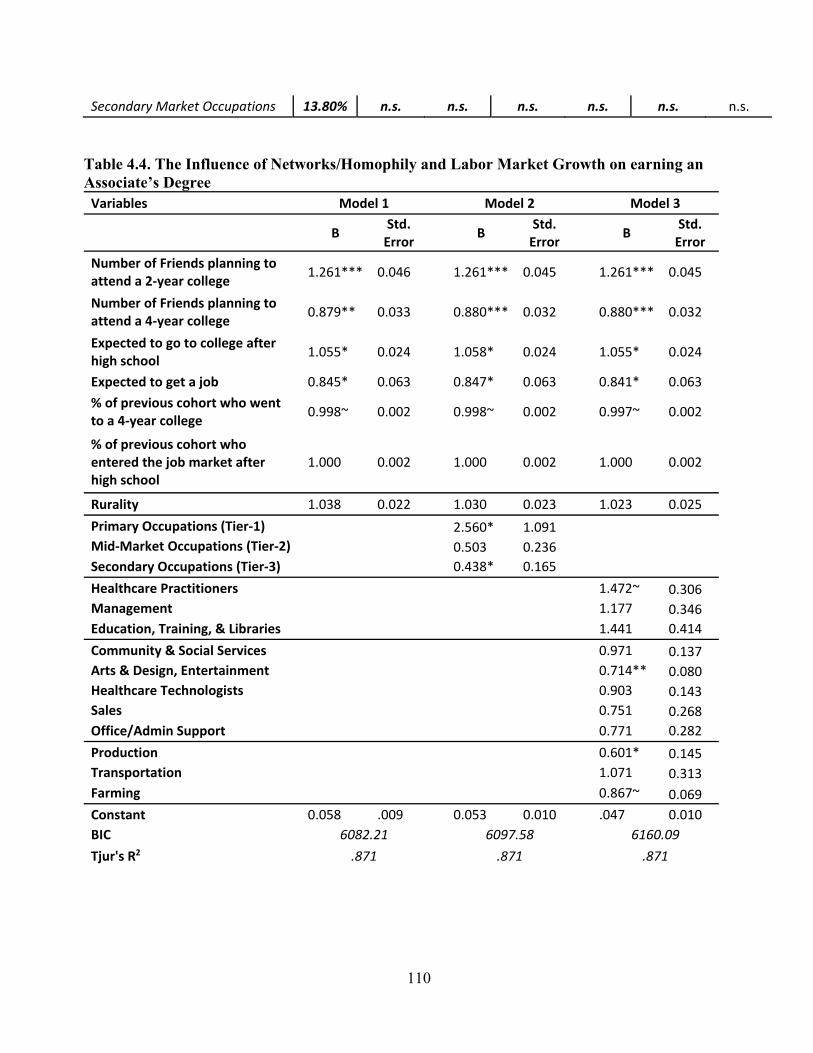
110

Secondary Market Occupations 13.80% n.s. n.s. n.s. n.s. n.s. n.s. Table 4.4. The Influence of Networks/Homophily and Labor Market Growth on earning an Associate’s Degree Variables Model 1 Model 2 Model 3

B Std. Error B Std.

Error B Std. Error


Number of Friends planning to attend a 4‐year college 0.879** 0.033 0.880*** 0.032 0.880*** 0.032

Expected to go to college after high school 1.055* 0.024 1.058* 0.024 1.055* 0.024

Expected to get a job 0.845* 0.063 0.847* 0.063 0.841* 0.063 % of previous cohort who went to a 4‐year college 0.998~ 0.002 0.998~ 0.002 0.997~ 0.002


1.000 0.002 1.000 0.002 1.000 0.002

Rurality 1.038 0.022 1.030 0.023 1.023 0.025 Primary Occupations (Tier‐1) 2.560* 1.091 Mid‐Market Occupations (Tier‐2) 0.503 0.236

Secondary Occupations (Tier‐3) 0.438* 0.165 Healthcare Practitioners 1.472~ 0.306 Management 1.177 0.346 Education, Training, & Libraries 1.441 0.414 Community & Social Services 0.971 0.137 Arts & Design, Entertainment 0.714** 0.080 Healthcare Technologists 0.903 0.143 Sales 0.751 0.268 Office/Admin Support 0.771 0.282 Production 0.601* 0.145 Transportation 1.071 0.313 Farming 0.867~ 0.069 Constant 0.058 .009 0.053 0.010 .047 0.010 BIC 6082.21 6097.58 6160.09

Tjur's R2 .871 .871 .871

111

Table 4.5. Summary of Factors Influencing Associate’s Degree Attainment, 90% Confidence Intervals

Networks & Homophily 1 Avg. A few Friends (1) Some Friends (2) Most Friends (3) Lower Upper Lower Upper Lower Upper


Number of Friends planning to attend a 4‐year college 3.37 ‐17.20% ‐6.60% ‐34.40% ‐13.20% ‐51.60% ‐19.80%




Expected to get a job 0.15 ‐25.70% ‐2.70% ‐77.10% ‐8.10% ‐154.20% ‐16.20%



% of previous cohort who went to a 4‐year college

44.50% ‐0.15% ‐0.01% ‐0.30% ‐0.01% ‐0.45% ‐0.02%


11.33% n.s. n.s. n.s. n.s. n.s. n.s.


Healthcare Practitioners ‐‐ 0.04% 1.07% 0.40% 10.70% 4.00% 107.00%

Arts & Design, Entertainment ‐‐ ‐0.33% ‐0.11% ‐3.30% ‐1.10% ‐33.00% ‐11.00% Production ‐‐ ‐0.84% ‐0.13% ‐8.40% ‐1.30% ‐84.00% ‐13.00% Farming ‐‐ ‐0.24% ‐0.01% ‐2.40% ‐0.10% ‐24.00% ‐1.00% Primary Market Occupations ‐‐ 0.28% 5.20% 2.80% 52.00% 28.00% 520.00% Mid‐level Market Occupations ‐‐ n.s. n.s. n.s. n.s. n.s. n.s. Secondary Market Occupations ‐‐ ‐0.74% ‐0.18% ‐7.40% ‐1.82% ‐74.00% ‐18.20%

112

Table 4.6. The Influence of Networks/Homophily and Labor Market Growth on earning a Bachelor’s Degree Variables Model 1 Model 2 Model 3

B Std. Error B Std.

Error B Std. Error



Expected to go to college after high school 1.145*** 0.015 1.146*** 0.015 1.146*** 0.015

Expected to get a job 0.689*** 0.053 0.690*** 0.052 0.690*** 0.052 % of previous cohort who went to a 4‐year college 1.005*** 0.001 1.004*** 0.001 1.004*** 0.001


0.996* 0.002 0.997* 0.002 0.996* 0.002

Rurality 0.970* 0.013 0.982 0.014 0.986 0.015 Primary Occupations (Tier‐1) 1.448 0.403 Mid‐Market Occupations (Tier‐2) 0.506* 0.163

Secondary Occupations (Tier‐3) 1.494~ 0.342 Healthcare Practitioners 1.002 0.144 Computers & Mathematics 0.941 0.056 Architecture & Engineering 1.100 0.109 Management 0.966 0.209 Business & Finance 0.992 0.150 Education, Training, & Libraries 1.054 0.202 Community & Social Services 1.001 0.094 Arts & Design, Entertainment 1.067 0.081 Healthcare Technologists 0.942 0.092 Sales 1.133 0.301 Office/Admin Support 0.853 0.227 Production 0.898 0.129 Personal Care 1.130 0.138 Construction/Extraction 0.926 0.110 Farming 1.103~ 0.057 BIC 13658.27 13679.99 13723.73

R2 .39 .39 .39

113

Table 4.7. Summary of Factors Influencing Bachelor’s Degree Attainment, 90% Confidence Intervals

Networks & Homophily 1 Avg. A few Friends (1) Some Friends (2) Most Friends (3)


Number of Friends planning to attend a 2‐year college 2.42 ‐0.16% ‐0.08% ‐0.31% ‐0.16% ‐0.47% ‐0.25%





Expected to get a job 0.15 ‐0.31% ‐0.20% ‐0.92% ‐0.60% ‐1.83% ‐1.19%



% of previous cohort who went to a 4‐year college 44.50% 0.50% 1.50% 1.00% 3.00% 1.50% 4.50%


11.33% ‐0.01% ‐0.0010% ‐0.01% ‐0.0020% ‐0.02% ‐0.0030%

Occupations Avg. Change per 1% Increase Change per 10%

Increase Change per 100%

Increase Lower Upper Lower Upper Lower Upper

Farming 0.01% 0.20% 0.10% 2.00% 1.00% 20.00%

Primary Market Occupations ‐‐ n.s. n.s. n.s. n.s. n.s. n.s. Mid‐level Market Occupations ‐‐ ‐0.63% ‐0.05% ‐6.31% ‐0.49% ‐63.10% ‐4.90% Secondary Market Occupations ‐‐ 0.01% 1.20% 0.10% 12.00% 1.00% 120.00%

114

Table 4.8. Summary of Factors Influencing Degree Attainment, 90% Confidence Intervals High School Associate’s Degree Bachelor’

Networks & Homophily 1 Avg. A few Friends A few Friends (1) A few Friends


Number of Friends planning to attend a 2‐year college 2.42 0.80% 20.00% 18.90% 33.40% ‐0.16% ‐0.08%

Number of Friends planning to attend a 4‐year college 3.37 39.20% 65.80% ‐17.20% ‐6.60% 33.70% 45.90%

Networks & Homophily 2 Avg. 1 network tie 1 network tie 1 network tie



Expected to get a job 0.15 n.s. n.s. ‐25.70% ‐2.70% ‐0.31% ‐0.20%



% of previous cohort who went to a 4‐year college 44.50% 47.50% 75.00% ‐0.15% ‐0.01% 0.50% 1.50%


11.33% 37.50% 92.50% n.s. n.s. ‐0.01% ‐0.0010%


Management 18.1% 0.21% 6.04% n.s. n.s. n.s. n.s. Healthcare Practitioners 36.4% n.s. n.s. 0.04% 1.07% n.s. n.s. Arts & Design, Entertainment 11.6% n.s. n.s. ‐0.33% ‐0.11% n.s. n.s. Production ‐19.0% n.s. n.s. ‐0.84% ‐0.13% n.s. n.s. Farming 16.7% n.s. n.s. ‐0.24% ‐0.01% 0.01% 0.20% Food Preparation & Service 31.9% ‐0.84% ‐0.13% n.s. n.s. n.s. n.s. Primary Market Occupations 22.20% 0.11% 9.20% 0.28% 5.20% n.s. n.s. Mid‐level Market Occupations 4.20% n.s. n.s. n.s. n.s. ‐0.63% ‐0.05% Secondary Market Occupations 13.80% n.s. n.s. ‐0.74% ‐0.18% 0.01% 1.20%

115

CHAPTERV

DISCUSSION/CONCLUSION

Utilizing Human Capital theory and Dual Labor Market theory, this study attempts to

answer six questions addressing the relationship between job growth in primary, mid-level,

and secondary labor markets and their impact on human capital development. Specifically:

1. Does employment growth in primary market occupations stimulate growth in the number

of high school graduates and college degree earners? 2. Given (1) is verified, how does the

impact of employment growth in primary occupations compare to midlevel and secondary

market occupations? 3. Does employment growth in primary market occupations influence

the probability of respondents graduating high school and/or earning a college degree? 4.

Given (3), how does the impact of employment growth in primary occupations compare to

the impact of growth in lower-tiered occupations? 5. Does employment growth in primary,

mid-level, and secondary market occupations influence the probability of graduating high

school and/or earning a degree when controlling for network/homophily effects? 6. Do

occupations illustrated to affect regional growth/decline in the number of degree earners

translate into an increased/decreased probability of earning a degree among individuals?

Overall, aggregate and respondent-level analyses illustrate two separate stories as to the

role of local labor market conditions in the development of human capital. At the county-

level, employment growth within primary, midlevel, and secondary markets was shown to

influence aggregate human capital development via an increased volume of credential

residents. Network/homophily factors, however, are better predictors of individuals’ degree

attainment. Each will be addressed in turn.

116

Utilizing a series of log-log regression models, change in counties’ volume of high school

and college educated residents was in part, shown to be dependent on employment growth in

local markets. From table 3.2, job development within primary, midlevel, and secondary

markets positively impacts growth in counties’ stock of high school graduates/G.E.D.

earners. Among the three tiers, employment growth in midlevel occupations was

significantly more influential compared to primary and secondary markets; predicted to

increase the volume of graduates by an average of .327% for each percentage increase in

employment. The impact of primary and secondary market growth was statistically identical.

This suggests employment opportunities in medium-wage occupations are more of an

incentive to finish secondary school than high-wage or low-wage occupations. In hindsight,

this is somewhat intuitive as occupations within primary markets typically require education

beyond high school while many secondary market jobs do not require their employees to

graduate or earn a G.E.D. From table 2.1, the highest degree earned by persons employed

within midlevel market occupations leans towards high school completion or the equivalent.

Parsed out by occupations, many were shown to stimulate growth in the number of high

school graduates. Within primary markets, employment growth within management and

education were positively influential while growth in life, physical, and social sciences;

architecture and engineering; and business and finance were negatively influential. As with

model 2, the negative impact of the latter occupations likely reflects the need for additional

education to fill job vacancies within these fields. As such, those whose highest education

level of education is the equivalent of a high school degree are not incentivized by these

occupations. In turn, employment growth in life sciences, architecture, etc. may lead to a

decrease in counties’ stock of college-educated residents. Within midlevel and secondary

117

markets, growth within most occupations increased the volume of residential high school

graduates.

In table 3.5, all occupational tiers were shown to increase the volume of Associate’s

degree earners. Here though, primary and midlevel market growth were shown to have

roughly the same impact, suggesting local and/or regional job opportunities in both medium

and high-wage occupations may incentivize 2-year degree attainment. Job development

within secondary markets was shown to negatively impact the volume of Associate’s degree

earners; suggesting local secondary market expansion may not incentivize local/regional

residents to pursue education beyond high school, since these occupations typically do not

require a 2-year degree.

Parsed out by occupations, the impact of each generally reflected the influence of the

aggregate tier it fell under. For example, primary market job growth has a strong, positive

impact on the volume of Associate’s degree earners, projected to increase it by .337% per

percentage of employment growth. The influence of the four primary market occupations

found to significantly impact the number of college educated residents, was also shown to be

positive. Within all three tiers, job growth in the entertainment industry was the only

exception to the rule, generating negative growth while gains in midlevel market

employment generate positive growth.

In table 3.8, all three occupational tiers were once again shown to influence degree

attainment, this time change in the number of persons with a Bachelor’s degree. Overall, job

growth within primary markets had the strongest effect, predicted to increase the volume of

college graduates by .528% for each percentage increase in employment. Comparatively, the

impact of midlevel markets was predicted to be .319%. A significant difference test verified

118

the slope effect of primary market growth was indeed greater than midlevel market growth,

producing a z-score of 6.554. As one may suspect, secondary market job growth had a net

negative impact on the volume of residential college graduates, predicted to decrease growth

by .117% per percentage increase in employment.

Parsed out by occupations, most job types were reflective of their respective tier. For

example, all significant primary and midlevel occupations had the same direction of effect as

primary and midlevel markets. Also worth noting is that two midlevel market occupations—

specifically sales and office/administrative support—had statistically identical slope effects

as management, a primary market occupation. This suggests that while growth in midlevel

markets, as a whole, may not have the same impact on the volume of college educated

residence, local/regional job opportunities within a few midlevel occupations may incentivize

Bachelor’s degree attainment. Within secondary markets, job growth in personal care was

the only significantly influential occupation to positively affect aggregate human capital

development. As mention previously, this is not likely due to the level of education required

to get a job within the field of personal care. Instead, this likely stems from the demand for

the services provided by persons employed in personal care—daycare, hospice care, etc.

In table 3.11, the 90% confidence intervals for all occupations found to significantly

influence aggregate human capital development are presented. Echoing results from tables

3-2, 3-5, and 3-8, the potential impact of employment growth varies by labor market,

occupation type, and degree of interest. Also of note, the amount of employment growth

required to produce sizable increases/decreases in the volume of residential degree earners is

substantial. Regarding high school, a doubling of employment in management, for example,

was predicted to increase the volume graduates by 5.7% - 9.4%. For reference, recall from

119

table 3.1 the mean growth in employment within management positions between 2000 and

2014 was 9.5%. This translates to about a .2% - 1.0% increase in degree earners. A similar

pattern occurs when considering other degree-types. A doubling of employment in

office/administrative support was projected to increase the volume of Associate’s degree

recipients by 14.9% - 22.7%, yet average growth for the industry stood at -1.6%; a doubling

of employment in education was projected to increase the volume of Bachelor’s degree

earners by 15.6% - 19.5%, yet average growth was 9.7%. Collectively, this suggests that

while employment growth within primary, midlevel, and secondary labor markets—and the

jobs there within—may influence the type of degree local/regional residents ultimately earn,

the effect size can be quite small.

After accounting for the effects of employment growth on aggregate human capital

development, occupational tiers as well was the job types found to be significantly influential

were transferred to a series of logistic models as a means of analyzing the influence of local

labor markets on individuals’ education outcomes. In addition, the influence of social

networks/homophily was also included such that the impact of local market conditions and

social ties could be compared. Overall, job growth in primary market occupations increased

the probability of respondents graduating high school and earning an Associate’s degree, but

had no bearing on Bachelor’s degree attainment.

From table 4.2, job creation within local primary markets had a substantial impact on the

odds of graduating high school; the likelihood projected to increase by an average of 2.26%

for each percent of employment growth. Increases/declines in midlevel and secondary

markets were not significantly influential. Parsed out by occupations, job growth in

management, business & finance, and food services were illustrated to affect high school

120

graduation, the latter of the three in a negative fashion. This suggests growth within primary

markets may incentivize students to finish high school and possibly move on to college. In

addition, whereas job growth within secondary labor markets was not influential, growth in

specific fields might be. From table 2.1, nearly a quarter of workers employed in the food

and services industry have not graduated high school nor earned a G.E.D., thus if fast food

occupations are all that is locally available, residents may not feel the need to finish high

school—they can find employment without it.

The influence of social networks/homophily on high school graduation was readily

apparent. If respondents’ friends had college ambitions, they were more likely to finish high

school. In addition, if students felt as though their family, friends, peers, etc. expected them

to go to college, they were more likely to do so. Further, if members of the previous

graduating cohort enrolled in college or entered the labor market, respondents were again,

more likely to graduate.

Regarding Associate’s degree attainment (table 4.4), job growth within primary and

secondary markets were significantly influential factors; with the former associated with

increased odds, the latter with decreased odds. When labor markets were parsed out by

occupations found to influence aggregate human capital development, job growth within the

healthcare industry was positively associated with earning a 2-year degree, projected to

increase the odds by as much as 1.07% for each percent of employment growth. Further

development of the arts & entertainment industry, production, and farming reduced the odds.

Once again, networks/homophily were found to be substantially influential, though unlike

their impact on high school graduation, a few factors had a negative impact. For example,

the odds of earning a 2-year degree increased if respondents’ friends planned to enroll in

121

community college, but declined if they planned to enroll at a 4-year university. Similarly,

the odds decreased if the previous graduating cohort tended to enroll at 4-year universities.

The same affect occurs in regards to the desires and expectations of others, with the odds of

earning a degree increasing if respondents felt as though they were expected to go to college,

yet decreased if they believed their family, friends, peers, etc. expected them to get a job after

graduating high school.

From table 4.6, employment growth within midlevel and secondary markets were found

to influence the odds of earning a Bachelor’s degree, yet only one occupation was found to

be influential. Regarding midlevel markets, job growth had a net negative effect on college

graduation, projected to decrease the odds by an average of .494% for each percent of job

growth. Counterintuitively, development of secondary markets was found to be positively

influential while primary market growth did not have an effect. These two phenomena may

be linked, however. Bachelor’s seekers maybe incentivized by perceived job opportunities

outside of their local region due to the overabundance of low-wage occupations.

Bachelor’s degree attainment was also shown to be affected by respondents’ social

networks. If a respondent’s friends planned to enroll in community college, (s)he was less

likely to earn a Bachelor’s degree, yet if they planned to enroll at a 4-year university, (s)he

was more likely to earn a Bachelor’s. The same pattern occurs when considering the desires

and expectations of others as well as the actions of the previous graduate cohort. If

respondents believed their family members, peers, etc. preferred them to go to college; they

were more likely to attain a 4-year degree. If they felt they were expected to enter the job

market, they were less likely to finish college. Likewise, if the previous graduating cohort

122

went to college, respondents were more likely to go to college; if the cohort entered the work

force, respondents were more likely to enter the workforce.

Across all logistic models, the influence of job growth was shown to fluctuate to a large

degree. From table 4.5, for example, development within primary markets was projected to

increase the odds of earning an Associate’s by .28% - 5.2% per percentage increase in

employment. Secondary market development is projected to decrease the odds by .18% -

.74%. Held at the county average, this means the projected odds of a respondent earning 2-

year degree increases by 6.2% - 115.4% due to employment growth in the local primary

market. Corollary, the odds are reduced by 4.0% - 16.4% due to employment growth in the

local secondary market. As such, nothing concrete can be said about the influential

magnitude of primary and secondary markets on earning an Associate’s; only that the former

is positively influential, while the latter is negatively influential. This pattern is pervasive

across all models of educational attainment.

Overall, it is difficult to say whether the expansion of job opportunities is as influential

on individuals’ human capital decisions as the company they keep. The volume of growth

required to increase respondents’ prospects of finishing high school and/or earning a college

degree can be substantial and the magnitude of effect can range considerably. A 1.0%

increase in employment within local primary markets, for example, is projected to increase

the odds of earning an Associate’s degree by .28% - 5.2%. Network factors obviously play a

large role, yet the extent of their potential effect is artificially limited by the number of

persons in respondents’ networks they were asked about. If we consider “Networks &

Homophily 2” in tables 4-3, 4-5, and 4-7 the upper limit is 6 ties. Further, the range of

persons in ego’s network is limited to parents, close relatives, close friends, favorite teachers,

123

and the school guidance counselor. The number and variety of potentially influential persons

within respondents’ networks is likely greater than 6. That said, the odds of earning a 2-year

degree are projected to increase by 1.67% - 9.4% for each tie respondents felt expected them

to enroll in college.

If changes in Tjur’s R2 and the BIC are used as the yardstick to determine whether

perceived opportunity or networks/homophily have a greater impact on respondents’ human

capital decisions; the latter would be preferable. Across all models measuring their

association with high school graduation, earning an Associate’s degree, and earning a

Bachelor’s degree; the R2 value remained static while the BIC increased when market and

occupation variables were added. In addition, the value and significance of coefficients for

all network variables remained virtually unchanged when labor market characteristics were

included. This suggests that while local job growth may play a small role in respondents’

education outcomes, it does not provide any additional explanatory power compared to

network/homophily effects.

HypothesesRevisited

Evidence for the first hypothesis—that job growth in primary market occupations will

generate more high school graduates, Associate’s degree earners and Bachelor’s degree

earners—was confirmed via models of aggregate human capital growth in Chapter III. By

and large, Employment growth within primary labor markets was positively associated with

human capital growth. In addition, the amount of growth with which they were associated

generally increased monotonically with the type of degree assessed. Whereas the overall

influence of job growth was positively related to high school graduation, the amount of

human capital growth it accounted for was somewhat larger for 2-year and 4-year degree

124

earners. This suggests that job growth in high-wage, high-skill jobs are a catalyst for

regional human capital growth, whether it stems from the local populous furthering their

education or migrants.

The second hypothesis—job growth in primary market occupations will generate a

larger increase in Associate’s degree and Bachelor’s degree earners, compared to the mid-

level and secondary job markets—was partially supported. Whereas increased employment

opportunities in primary markets generated more human capital growth via the number of 4-

year degree holders, it generated fewer Associate’s degree earners compared to midlevel

markets. In hindsight, this makes sense as primary market jobs generally require “primary

market degrees,” as illustrated in table 2.1. This too, suggests people tend to strike

equilibrium between their own human capital investment and the types of occupations

available to them. If local job growth predominantly occurs within mid-level market

occupations, employment seekers will adjust their time and money investments to

compensate, i.e., obtain the degree of education required by most jobs available to them.

Whereas the first two hypotheses tested the relationship between local job growth and

aggregate human capital development, hypotheses three through five tested the effects of

local job growth on the probability of graduating high school and/or earn a college degree.

Evidence for hypothesis three— employment growth within primary market occupations will

increase the probability of graduating high school, earning an Associate’s degree, and/or

earning a Bachelor’s degree —was partially supported. Whereas primary market growth was

positively associated the odds of graduating high school and earning an Associate’s, it did

not influence Bachelor’s degree attainment. This may suggest local labor markets are not the

125

only consideration taken into account when deciding to pursue a 4-year degree. Regional,

state, and nation job opportunities may also be c.

Hypothesis four—employment growth in primary job markets will induce a higher

likelihood of earning an Associate’s degree and Bachelor’s degree compared to job growth in

the mid-level and secondary job markets—is partially supported, though with a few caveats.

First, employment growth in midlevel job markets were not significant predictors of

Associate’s degree attainment and was negatively associated with earning a Bachelor’s

degree. Second, while primary market growth did not significantly impact the odds of

earning a Bachelor’s, secondary market growth was positively associated though the effect

was marginal. It is also worth noting that primary market growth had a positive impact on the

odds of high school completion while midlevel and secondary markets where not influential.

Hypothesis five—Social Networks/Homophily will impact students’ education outcomes

—is also supported. Overall, the majority of network variables significantly influenced the

likelihood of graduating high school, earning an Associate’s degree, and earning a Bachelor’s

degree. Respondents were malleable to the influences and/or desires of the people around

them regarding decisions on their own human capital. In addition, the company respondents

kept proved more influential than local employment growth in high-wage, high-skill

occupations. In fact, adding employment variables did not increase the predictive power of

the base model, as indicated by the Tjur’s R2 statistic and the increased BIC. This suggests

that local employment changes by occupation, at best, play a minor role in individuals’

decisions pertaining to human capital development.

Finally, how does the association between aggregate primary market job growth and

aggregate human capital development compare to the behaviors of individuals? Overall,

126

primary market growth was illustrated to affect growth in the number of residential high

school graduates, Associate’s degree earners, and Bachelor’s degree earners. At the

individual level, it only affected the odds of high school completion. Additionally, whereas

growth within mid-level and secondary job markets where found to positively influence

counties’ stocks of high school graduates, neither affected the likelihood of residents

graduating high school. This suggests the bump in human capital was primarily due to

migration. Local job growth in midlevel markets was shown to positively affect the number

of college degree earners, yet did not affect the odds of respondents earning an Associate’s

and a negative effect on earning a Bachelor’s. This too, suggests much of counties’ increase

in human capital between 2000 and 2014 was primarily due to migration, not the conditions

of local markets themselves.

Improvements&Discussion

Several steps could be taken to strengthen the results of this analysis. Concerning data, it

would be beneficial to include measures of parental involvement in respondents’ educational

trajectories. If parents’ involvement in the education process effects whether their children

finish high school, enroll in college, earn an Associate’s or Bachelor’s, it may also affect

what respondents view as incentives to enter the job market. Further, data as to whether any

of the survey respondents’ network ties have leads on job opportunities would also be

beneficial. It is entirely possible that respondents who opt out of college still have access to

well-paying jobs despite local market conditions.

In addition, the present study would likely benefit from changes to the modeling

procedure. First, instead of measuring the impact of employment change from time A to time

B, it may be more beneficial to assess the impact from A to B to C to D, etc. The assessment

127

of market influences on respondents’ educational outcomes at multiple points in time would

be ideal as it would allow for the inclusion of factors which may be time sensitive and/or

“life events.” For example, respondents may not immediately enroll in college after high

school graduation and opt for employment instead. Should the job be lost, respondents may

pursue a college degree to increase their chances of obtaining a better occupation and

decrease the likelihood of unemployment in the future. In addition, life events such as

marriage, child birth, etc. may delay college entry and degree attainment once enrolled.

Further, market conditions may interact of life events to drastically increase or decrease the

likelihood of earning a degree. For example, persons living in rural areas with limited work

options may choose to enroll in college as a means of supporting themselves and their

dependents, whereas new parent(s) in areas with diverse job options may choose to work

instead.

This study could also benefit from hierarchical nesting which would permit the

assessment of market conditions at multiple levels of aggregation. This could illuminate

“which” job opportunities in “what” markets incentivize college attendance and/or the

pursual of a degree. For students pursuing a Bachelor’s within highly specialized fields, job

opportunities in the county might not matter as much as those within county groups, the

region, the state, or the US. If students from rural, landlocked areas want to go into

oceanography, they would not consider the local market as a viable option. In a hierarchical

time-series model, the market conditions at each level of aggregation could be modeled

overtime.

Results of this study carry some education policy implications, particularly when it

comes to the phenomenon dubbed “brain drain,” the tendency of young, college educated

128

persons to leave rural, underdeveloped areas. Results indicate growth in primary market

occupations has a positive effect on the likelihood of finishing high school and earning an

Associate’s degree yet growth in secondary markets had a negative impact on the later. This

suggests local governments should be mindful of the industries permitted to enter the area. If

the goal is to develop and improve market conditions such that young, educated youths will

remain in the county, region, state, etc.—further generating the manpower and skills

necessary to improve the local economy—emphasis should be placed on increasing job

opportunities in primary labor markets. Further, less emphasis should be placed on

secondary market industries such as production and farming. Policy makers should be wary

of giving tax incentives as a means of attracting car assembly plants, textile mills, warehouse

distribution centers, etc. and instead opt to recruit companies dedicated to healthcare, the

sciences, and education. Ideally, this would reduce the degree of regional brain drain and

increase the overall quality of residential life.

129

APPENDIXA

DESCRIPTIONOFOCCUPATIONS

Management Occupations: Jobs in management span all 23 ACS occupational

categories. This includes chief executives of companies, financial managers, transportation,

storage and distribution managers, farm managers, construction managers, education

administrators, funeral directors, etc. In short, occupations classified as “Management”

involve the oversight and guidance of employees. Additionally, management positions are

not categorized with their respective occupational groups. For example, farm managers are

not classified as both management occupations and farm occupations. They are classified

only as the former. Compared to other occupational categories, management jobs received

the highest desirability score, ranking of 6.

Business and Finance Occupations: Occupations within business and finance range

from credit, budget, and personal finance advisors to market analysts, logisticians, claims

adjusters, and cost adjusters, etc. In terms of desirability, occupations in business and

finance are ranked 7th.

Computer and Mathematical Occupations: Computer and mathematical occupations

include mathematicians, statisticians, web developers, database administrators, systems

analysts, etc. Computer and mathematical occupations are ranked 4th, in terms of

desirability.

Architecture and Engineering Occupations: Mechanical engineers, civil engineers,

chemical engineers, surveyors, cartographers, drafters, etc. are examples of job types

categorized as Architecture and Engineering occupations. Of note, though computer

hardware engineers are included in this category, they are not categorized as a “Computer

130

and Mathematical Occupation.” Architecture and engineering jobs received a desirability

ranking of 5th.

Life, Physical, and Social Science Occupations: Jobs in this category emphasize

research. Occupations range from biology, geology, chemistry, astronomy, and physics to

sociology, psychology, and econometrics. As measured, Life, physical, and social science

occupations are the 3rd highest ranking category.

Community and Social Services Occupations: Community and social services jobs

include councilors, social workers, probation officers, clergy, and other religious workers.

Occupations within this category have an aggregated desirability ranking of 8th out of 23.

Legal Occupations: Lawyers, judges, magistrates, paralegals, etc. are categorized as

legal occupations. Legal Occupations are the highest ranked occupational category in terms

of income and the educational attainment of its workforce.

Education, Training, and Library Occupations: Most occupations falling under this

category are involved with K-12 education, including elementary and middle school teachers,

high school teachers, teacher assistants, librarians, etc. Jobs within the education industry are

collectively ranked 8th out of 23.

Arts, Design, Entertainment, Sports, and Media Occupations: Jobs within this area

are largely within the entertainment industry. These occupations include athletes, singers,

songwriters, dancers, news anchors, actors, writers, authors, etc. In terms of desirability, jobs

within entertainment are ranked 10th.

Health Practitioner Occupations: Health practitioners include dentists, doctors, nurses,

physical therapists, speech pathologists, dieticians, optometrists, etc. Of note, health

practitioners does not include health technologists or health support staff, both of which are

131

their own designated categories. Occupations classified as “Health Practitioner” are ranked

2nd in terms of desirability.

Health Technology Occupations: Health technology occupations include clinical lab

technicians, emergency medical technicians (EMTs), and other technical positions not

including health practice or diagnosis. Health Technology Occupations received a

desirability rank of 11.

Health Support Occupations: By and large, persons holding jobs that are categorized as

“Health Support” do not perform health diagnoses. Instead, they occupy positions such as

home health aides, massage therapists, medical assistants, pharmacy aides, etc. Compare to

other occupational categories included in this analysis, health support occupations are in the

lower spectrum of desirability ranking of 16.

Protective Service Occupations: People employed in protective services include police

officers, firefighters, corrections officers, animal control workers, detectives, lifeguards, and

moreorless any occupation that involves public safety (sans healthcare). The protective

services industry is in “the middle of the pack” in terms of its desirability score, with a rank

of 12.

Food Preparation and Service Occupations: Bartenders, dishwashers, waiters,

waitresses, cooks, and any occupation that involves servicing the public foodstuffs fall into

this category. Compared to other occupational categories, food preparation received the

lowest desirability rank with a score of 21.

Building and Grounds Cleaning/Maintenance Occupations: Janitors, maids,

housekeepers, and pest control workers constitute the majority of jobs in this category.

132

Maintenance occupations are near the bottom of the hierarchy in terms of desirability with a

ranking of 22.

Personal Care and Service Occupations: Flight attendants, personal care aides, barbers,

hairdressers, tour guides, other recreation workers, etc. are classified into this category.

Personal care occupations are ranked in the lower quartile regarding desirability, with a rank

of 19.

Sales and Related Occupations: As suggested by its name, “sales and related

occupations” consists primarily of retail jobs, such as cashier, telemarketer, travel agent,

advertising, street vendor, insurance salesman, etc. Sales occupations scored a desirability

rank of 13 out of 23.

Office and Administrative Support Occupations: The spectrum of jobs in this category

is vast, but the common theme among them is that they consist of clerks, assistants, as well as

other jobs that were once labeled “pink-collar.” Occupations range from data entry, account

clerks, office clerks, mail clerks, library assistants, secretaries, dispatchers, etc. Office and

administrative support occupations received a ranking of 14 out of 23.

Farming, Fishing, and Forestry Occupations: Logging, fishing, hunting, forest

conservation, agricultural inspectors, etc. are lumped into this category. Compared to other

occupations, jobs like these generally do not require education beyond high school, nor do

they command a large salary, evidenced by their aggregate desirability ranking; 23 out of 23.

Construction and Extraction Occupations: Persons whose primary job is in anyway

related to construction fall into this category. This includes occupations such as carpentry,

dry walling, stone masonry, roofing, sheet-metal work, elevator installation, boiler making,

highway maintenance, etc. Though the type of labor involved is not related to construction,

133

mining is also included. Overall, jobs classified as “Construction and Extraction” have a

score of 20 out of 23.

Installation and Repair Occupations: Occupations such as small engine repair, aircraft

mechanics, home appliance repair, power-line installation and repair, etc. are grouped into

this category. These types of jobs received a desirability rank of 15 out of 23.

Production Occupations: Among all ACS occupational groupings, production jobs are

the most varied, ranging from motor assembly, print binding, and upholstery to baking,

tobacco roasting, and jeweler/precious stone worker. Despite the variability of job types

within this category, collectively production occupations received a rank of 17 out of 23.

This is likely due to the fact that most production jobs do not require an extensive skill set or

pay well.

Transportation and Material Moving Occupations: Bus drivers, airplane pilots, train

operators, truck drivers, sailors, and any other job involving public transportation, or the

transportation of product, are grouped into this category. Transportation occupations

received a rank of 18 out of 23.

134

APPENDIXB

SOCIALNETWORKS/HOMOPHILYSURVEYITEMS

F1S44A: Mother’s desire for respondent after high school (mark all that apply). a) Go to college b) Get a full-time job c) Enter vocational/technical school or an apprenticeship d) Enter military service e) Get married f) They think I should do what I want g) I don’t know

F1S44B: Father’s desire for respondent after high school (mark all that apply). a) Go to college b) Get a full-time job c) Enter vocational/technical school or an apprenticeship d) Enter military service e) Get married f) They think I should do what I want g) I don’t know

F1S44C: Close relative’s desire for respondent after high school (mark all that apply). a) Go to college b) Get a full-time job c) Enter vocational/technical school or an apprenticeship d) Enter military service e) Get married f) They think I should do what I want g) I don’t know F1S44D: Friend’s desire for respondent after high school (mark all that apply). a) Go to college b) Get a full-time job c) Enter vocational/technical school or an apprenticeship d) Enter military service e) Get married f) They think I should do what I want g) I don’t know

135

F1S44E: School counselor’s desire for respondent after high school (mark all that apply). a) Go to college b) Get a full-time job c) Enter vocational/technical school or an apprenticeship d) Enter military service e) Get married f) They think I should do what I want g) I don’t know F1S44F: Favorite teacher’s desire for respondent after high school (mark all that apply). a) Go to college b) Get a full-time job c) Enter vocational/technical school or an apprenticeship d) Enter military service e) Get married f) They think I should do what I want g) I don’t know

F1S65C: How many of your friends plan to attend a 2-year community college?

a) None b) A few c) Some d) Most e) All F1S65C: How many of your friends plan to attend a 2-year community college?

a) None b) A few c) Some d) Most e) All

F1S65D: How many of your friends plan to attend a 4-year college/university?

a) None b) A few c) Some d) Most e) All

136

F1A19A: Percent of 2003 graduates who went to a 4-year college/university

a) None b) 1-10% c) 11-24% d) 25-49% e) 50-74% f) 75-100% F1A19C: Percent of 2003 graduates who entered the labor market after graduation

a) None b) 1-10% c) 11-24% d) 25-49% e) 50-74% f) 75-100%

137

REFERENCESCITED

Alcobendas, M.A., & Rodriguez-Planas, N. (2010). Immigrants’ Assimilation Process in a

Segmented Labor Market. Revised IZA Discussion Paper No. 4394.

Altonji, J.G., Blom, E., & Meghir, C. (2012). Heterogeneity in Human Capital Investments:

High School Curriculum, College Major, and Careers. Working Paper Series, National

Bureau of Economic Research: Cambridge, MA.

Anderson, Kathryn H., Butler, John S., & Sloan, Frank A. (1987). Labor Market

Segmentation: A Cluster Analysis of Job Groupings and Barriers to Entry. Southern

Economic Journal, 53(3), 571-590.

Angrist, J. D. & Lang, K. (2002). How Important are Classroom Peer Effects? Evidence

from Boston’s Metco Program. W.E. UpJohn Institute for Employment Research,

working paper no. 02-85.

Arcidiacono, P. & Nicholson, S. (2003). Peer Effects in Medical School. Journal of Public

Economics, 89(2-3), 327-50.

Astone, N. M. & McLanahan, S.S. (1991). Family Structure, Parental Practices, and High

School Completion. American Sociological Review, 56(3), 309-20.

Baum, S. & Payea, K. (2005). The Benefits of Higher Education for Individuals and Society.

Education Pays 2004: Trends in Higher Education Series, Report for the College Board.

Becker, Gary. (1994). Human Capital Theory (3rd Edition). University of Chicago Press.

138

Bedard, K. & Herman, D. A. (2006). Who Goes to Graduate/Professional School? The

Importance of Economic Fluctuations, Undergraduate Field, and Ability. Economics of

Education Review, 27(2), 197-210.

Belman, D. & Heywood, J.S. (1991). Sheepskin Effects in the Returns to Education: An

Examination of Women and Minorities. The Review of Economics and Statistics, 73(4),

720-24.

Betes, J.R. & McFarland, L.L. (1995). Safe Port in a Storm: The Impact of Labor Market

Conditions on Community College Enrollments. The Journal of Human Resources,

30(4), 741-765.

Black, D.A., McKinnish, T.G., & Sanders, S.G. (2005). Tight Labor Markets and the

Demand for Education: Evidence from the Coal Boom and Bust. ILR Review, 59(1),

Article 1.

Blaug, M. (1976). The Empirical Status of Human Capital Theory: A Slightly Jaundiced

Survey. Journal of Economic Literature, 14(3), 827-855.

Boston, T.D. (1990). Segmented Labor Markets: New Evidence from a Study of Four Race-

Gender Groups. Industrial and Labor Relations Review, 44(1), 99-115.

Bowen, H.R. (1996). Investing in Learning: The Individual and Social Value of American

Higher Education. Transaction Publishers, New Brunswick (USA) and London (UK).

Bozick, R. (2009). Job Opportunities, Economic Resources, and the Postsecondary

Destinations of American Youth. Demography, 46(3), 493-512.

139

Brenner, M.H. (1976). Estimating the Costs of National Economic Policy. Study prepared for

the Joint Economic Committee, U.S. Congress, 94th Congress, 2nd Session. Washington

DC: U.S. Government Printing Office.

Calvo-Armengol, A. & Patacchini, E. (2009). Peer Effects and Social Networks in Education.

The Review of Economic Studies, 76(4), 1239-1267.

Cairns, R.B., Cairns, B.D., & Neckerman, H.J. (1989). Early School Dropout: Configurations

and Determinants. Child Development, 60(6), 1437-52.

Carbonaro, W. & Workman, J. (2013). Dropping Out of High School: Effects of Close and

Distant Friendships. Social Science Research, 42, 1254-68.

Carbonaro, W. & Workman, J. (2016). Intermediate Peer Contexts and Educational

Outcomes: Do the Friends of Students’ Friends Matter? Social Science Research, 58,

184-97.

Catterall, J.S. (1987). On the Social Costs of Dropping out of School. The High School

Journal, 71(1), 19-30.

Davies, S. & Guppy, N. (1997). Fields of Study, College Selectivity, and Student Inequalities

in Higher Education. Social Forces, 75(4), 1417-1438.

Davis-Kean, P.E. (2005). The Influence of Parent Education and Family Income on Child

Achievement: The Indirect Role of Parental Expectations and the Home Environment.

Journal of Family Psychology, 19(2), 294-304.

Dickens, William T., & Lang, K. (1985). A Test of Dual Labor Market Theory. The

American Economic Review, 75(4), 792-805.

140

Dickens, WT., & Lang, K. (1988). The Reemergence of Segmented Labor Market Theory.

The American Economic Review, 78(2), 129-134.

DiMaggio, P. (1982). Cultural Capital and School Success: The Impact of Status Culture

Participation on the Grades of U.S. High School Students. American Sociological

Review, 47, 189-201.

DiMaggio, P. & Mohr, J. (1985). Cultural Capital, Educational Attainment, and Marital

Selection. American Journal of Sociology, 90(6), 1231-1261.

Doeringer, P.B., & Piore, M.J. (1971). Low-Income Labor Markets and Urban Manpower

Programs: A Critical Assessment. Research and Development Findings No. 12.

Washington: Department of Labor.

Doeringer, P.B., & Piore, M.J. (1971). Internal Labor Markets and Manpower Analysis. D.C.

Heath and Company, Lexington, MA.

Dubow, E.F., Boxer, P. & Huesmann, L. R. (2009). Long-term Effects of Parents’ Education

on Children’s Educational and Occupational Success: Mediation by Family Interactions,

Child Aggression, and Teenage Aspirations. Merrill Palmer Q (Wayne State University

Press), 55(3), 224-49.

Duflo, E., Dupas, P. & Kremer, M. (2011). Peer Effects, Teacher Incentives, and the Impact

of Tracking: Evidence from a Randomized Evaluation in Kenya. The American

Economic Review, 101(5), 1739-74.

Duncan, B. (1965). Dropouts and the Unemployed Journal of Political Economy, 73(2), 121-

134.

141

Duncan, O.D., Haller, A.O. & Portes, A. (1968). Peer Influences on Aspirations: A

Reinterpretation. American Journal of Sociology, 74(2), 119-37.

Egerton, M. (1997). Occupational Inheritance: The Role of Cultural Capital and Gender.

Work, Employment, and Society, 11(2): 263-282.

England, P. (1982). The Failure of Human Capital Theory to Explain Occupational Sex

Segregation. The Journal of Human Resources, 17(3), 358-370.

Farkas, G. (2003). Racial disparities and Discrimination in Education: What do we know,

how we know it, and what do we need to know? Teachers College Record, 105(6),

1119-1146.

Gittleman, M.B. & Howell, D.R. (1995). Changes in the Structure and Quality of Jobs in the

United States: Effects by Race and Gender, 1983-1990. Industrial and Labor Relations

Review, 48(3), 420-440.

Glasgow, K.L., Dornbusch, S.M., Troyer, L., Steinberg, L., & Ritter, P.L. (1997). Parenting

Styles, Adolescents’ Attributions, and Educational Outcomes in Nine Heterogeneous

High Schools. Child Development, 68(3), 507-529.

Goldin, C. & Katz, L.F. (2008). Why the United States Led in Education: Lessons from

Secondary School Expansion, 1910 to 1940. Presentation Paper, revised version of

NBER Working Paper no. 6144.

Graham, J. & Shakow, D.M. (1990). Labor Market Segmentation and Job-Related Risk:

Differences in Risk and Compensation between Primary and secondary Labor Markets.

The American Journal of Economics and Sociology, 49(3), 307-323.

142

Green, D.P. & Shapiro, I. (1994). Pathologies of Rational Choice Theory: A Critique of

Applications in Political Science. New Haven: Yale University Press.

Griffin, L.J., Kllenberg, A.L., & Alexander, K.L. (1981). Determinants of Early Labor

Market Entry and Attainment: A Study of Labor Market Segmentation. Sociology of

Education, 54(3), 206-221.

Halle, T., Krutz-Costes, B., & Mahoney J. (1997). Family Influences on School Achievement

in Low-Income, African American Children. Journal of Educational Psychology, 89,

527-537.

Hanushek. E.A., Kain, J.F., Markman, J.M. & Rivkin, S.G. (2003). Does Peer Ability Affect

Student Achievement? Journal of Applied Econometrics, 18(5), 527-44.

Harrison, B. & Sum, A. (1979). The Theory of ‘Dual’ or Segmented Labor Markets. Journal

of Economic Issues, 13(3), 687-706.

Heckman, J.J., & Hotz, V. (1986). An Investigation of the Labor Market Earnings of

Panamanian Males Evaluating the Sources of Inequality. The Journal of Human

Resources, 21(4), 507-542.

Hechter, M. & Kanazawa, S. (1997). Sociological Rational Choice Theory. Annual Review of

Sociology, 27, 191-214.

Hiebert, D. (1999). Local Geographies of Labor Market Segmentation: Montreal, Toronto,

and Vancouver. Economic Geography, 75(4), 339-369.

Hillman, N.W. & Orians, E.L. (2013). Community Colleges and Labor Market Conditions:

How Does Enrollment Demand Change Relative to Local Unemployment Rates?

Research in Higher Education, 54, 765-780.

143

Hollingshead, A.B. (1949). Elmtown’s Youth: The Impact of Social Classes on Adolescents,

John Wiley & Sons, Inc.

Hoxby, C.M. Peer Effects in the Classroom: Learning from Gender and Race Variation.

(2000). National Bureau of Economic Research, NBER Working Paper No. 7867.

Hudson, K. (2007). The New Labor Market Segmentation: Labor Market Dualism in the

New Economy. Social Science Research, 36, 286-312.

Ihlanfeldt, K.R. & Sjoquist, D.L. (1998). The Spatial Mismatch Hypothesis: A Review of

Recent Studies and Their Implications for Welfare Reform. Housing Policy Debate,

9(4), 849-892.

Jaeger, D.A. & Page, M.E. (1996). Degrees Matter: New Evidence on Sheepskin Effects in

the Returns to Education. The Review of Economics and Statistics, 78(4), 733-740.

Jepsen, C., Troske, K. & Coomes, P. (2012). The Labor-Market Returns to Community

College Degrees, Diplomas, and Certificates. University College Dublin School of

Economics, Working Paper Series, WP12/23.

Jimerson, S., Egeland, B., & Teo, A. (1999). A Longitudinal Study of Achievement

Trajectories: Factors Associated with Change. Journal of Educational Psychology,

91(1), 116-126.

Kain, J.F. (1992). The Spatial Mismatch Hypothesis: Three Decades Later. Housing Policy

Debate, 3(2), 371-392.

Kalleberg, A.L. & Sorensen, A.B. (1979). The Sociology of Labor Markets. Annual Review

of Sociology, 5, 351-379.

144

Kandel, D.B. (1978). Homophily, Selection, and Socialization in Adolescent Friendships.

American Journal of Sociology, 84(2), 427-36.

Kane, T.J. & Rouse, C.E. (1995). Labor-Market Returns to Two- and Four-Year College. The

American Economic Review, 85(3), 600-614.

Kaufman, R.L., Hodson, R., & Fligstein, N.D. (1979). Defrocking Dualism: A New Approach

to Defining Industrial Sectors. CDE Working Paper #80-1.

Krein, S.F., Beller, A.H. (1988). Educational Attainment of Children from Single-Parent

Families: Differences by Exposure, Gender, and Race. Demography, 25(2), 221-234.

Ladson-Billings, G. (2006). From the Achievement Gap to the Education Debt:

Understanding Achievement in U.S. Schools. Educational Researcher, 35(7), 3-12.

Leontaridi, M.R. (1998). Segmented Labour Markets: Theory and Evidence. Journal of

Economic Surveys, 12(1), 63-101.

Little, D. (1991). Rational-Choice Models and Asian Studies. The Journal of Asian Studies,

50(1), 35-52.

Luster, T., Rhoades, K., & Haas, B. (1989). The Relation between Parental Values and

Parenting Behavior: A Test of the Kohn Hypothesis. Journal of Marriage and the

Family, 51, 139-147.

Manski, C.F., & Wise, D.A. (1983). College Choice in America. Harvard University Press.

Marcotte, D.E., Bailey, T., Borkoski, C., & Kienzi, G.S. (2005). The Returns of a

Community College Education: Evidence from the National Education Longitudinal

Survey. Educational Evaluation and Policy Analysis, 27(2), 157-175.

145

Marquis, S.M., & Long, S.H. (2001). Employer Health Insurance and Local Labor Market

Conditions. International Journal of Health Care Finance and Economics, 1(3/4), 273-

292.

Mata, F., & Pendakur, R. (1999). Immigration, Labor Force Integration and Pursuit of Self-

Employment. The International Migration Review, 33(2), 378-402.

McCall, L. (2001). Sources of Racial Wage Inequality in Metropolitan Labor Markets:

Racial, Ethnic, and Gender Differences. American Sociological Review, 66(4), 520-541.

McLafferty, S. & Preston, V. (1992). Spatial Mismatch and Labor Market Segmentation for

African-American and Latina Women. Economic Geography, 68(4), 406-431.

McMahon, W.W. & Wagner, A.P. (1981). Expected Returns to Investment in Higher

Education. The Journal of Human Resources, 16(2), 274-285.

Mincer, J. (1958). Investment in Human Capital and Personal Income Distribution. Journal

of Political Economy, 66(4), 281-302.

Morgenstern, R.D. (1973). Direct and Indirect Effects on Earnings of Schooling and Socio-

Economic Background. The Review of Economics and Statistics, 55(2), 225-233.

Morissette, R., Chan, P.C.W. & Lu, Y. (2014). Wages, Youth Employment, and School

Enrollment: Recent Evidence from Increases in World Oil Prices. Statistics Canada,

Analytical Studies Branch Research Paper Series.

Neumark, D., & Wascher, W. (1995). Minimum Wage Effects on Employment and School

Enrollment. Journal of Business and Economic Statistics, 13(2), 199-206.

Oster, G. (1979). A Factor Analytic Test of the Theory of the Dual Economy. The Review of

Economics and Statistics, 61(1), 33-39.

146

Osterman, P. (1975). An Empirical Study of Labor Market Segmentation. Industrial and

Labor Relations Review, 28, 508-523.

Pennington, K.L., McGinty, D. & Williams, M.R. (2002). Community College Enrollment

as a Function of Economic Indicators. Community College Journal of Research and

Practice, 26(5), 431-437.

Perna, L.W. (2000). Differences in the Decision to Attend College among African

Americans, Hispanics, and Whites. The Journal of Higher Education, 71(2), 117-141.

Piore, M.J. (1972). Notes for a Theory of Labor Market Stratification. Working Paper.

Massachusetts Institute of Technology.

Polachek, S.W. (1975). Discontinuous Labor Force Participation and Its Effects on Women’s

Market Earnings. In Sex, Discrimination, and the Division of Labor, ed. Cynthia Lloyd.

New York: Columbia University Press, 1975. 137-57.

Polachek, S.W. (1976). Occupational Segregation: An Alternative Hypothesis. Journal of

Contemporary Business, 5, 1-12.

Polachek, S.W. (1979). Occupational Segregation Among Women: Theory, Evidence, and a

Prognosis. In Women in the Labor Market, eds. Cynthia Lloyd, Emily Adrews, and

Curtis Gilroy. New York: Columbia University Press.

Polachek, S.W. (1981). Occupational Self-Selection: A Human Capital Approach to Sex

Differences in Occupational Structure. The Review of Economics and Statistics, 63(1),

60-69.

Rees, D.I., & Mocan, H.N. (1997). Labor Market Conditions and the High School Dropout:

Evidence from New York State. Economics of Education Review, 16(2), 103-109.

147

Reich, M., Gordon, D.M., & Edwards, R.C. (1973). A Theory of Labor Market

Segmentation. The American Economic Review, 63(2), 359-365.

Reid, L.W., & Rubin, B.A. (2003). Integrating Economic Dualism and Labor Market

Segmentation: The Effects of Race, Gender, and Structural Location on Earnings. The

Sociological Quarterly, 44(3), 405-432.

Reimers, C.W. (1983). Labor Market Discrimination against Hispanic and Black Men. The

Review of Economics and Statistics, 65(4), 570-79.

Roksa, J. & Levey, T. (2010). What Can You Do with That Degree? Major and Occupational

Status of College Graduates over Time. Social Forces, 89(2), 389-415.

Rocigno, V.J. (1998). Race and the Reproduction of Educational Disadvantage. Social

Forces, 76(3), 1033-1061.

Rouse, C.E. (2005). The Labor Market Consequences of an Inadequate Education Prepared

for the Equity Symposium on “The Social Costs of Inadequate Education.”

Rumberger, R.W. (1983). Dropping out of High School: The Influence of Race, Sex, and

Family Background. American Educational Research Journal, 20, 199-220.

Rumberger, R.W. (1987). High School Dropouts: A Review of Issues and Evidence. Review

of Educational Research, 57(2), 101-121.

Sacerdote, B. (2001). Peer Effects with Random Assignment: Results for Dartmouth

Roommates. The Quarterly Journal of Economics, 681-704.

Sakamoto, A., & Chen, M.D. (1991). Inequality and Attainment in a Dual Labor Market

American Sociological Review, 56(3), 295-308.

148

Sakamoto, A., & Powers, D.A. (1995). Education and the Dual Labor Market for Japanese

Men. American Sociological Review, 60(2), 222-246.

Sewell, W.H. & Shah, V.P. (1968). Parents’ Education and Children’s Educational

Aspirations and Achievements. American Sociological Review, 33(2), 191-209.

Shultz, T.W. (1961). Investment in Human Capital The American Economic Review, 51(1),

1-17.

Smith, C.L. (2012). The Impact of Low-Skilled Immigration on the Youth Labor Market.

Journal of Labor Economics, 30(1), 55-89.

Song, C. & Glick, J. (2004). College Attendance and Choice of College Majors among

Asian-American Students. Social Science Quarterly, 85(5), 1401-1422.

Sum, A., Khatiwada, I., & McLaughlin, J. (2009). The Consequences of Dropping Out of

High School: Joblessness and Jailing for High School Dropouts and the High Cost for

Taxpayers. Center for Labor Market Studies Publications. Paper 23.

Stratton, L.S., O’Toole, D.M., & Wetzel, J.N. (2004). “Factors Affecting Initial Enrollment

Intensity: Part-Time Versus Full-Time Enrollment.” Economics of Education Review,

23, 167-175.

Thompson, J.P. (2009). “Using Local Labor Market Data to Re-examine the Employment

Effects of the Minimum Wage.” Industrial and Labor Relations Review, 62(3), 343-

366.

Tjur, T. (2009). “Coefficients of Determination in Logistic Regression Models—A New

Proposal: The Coefficient of Discrimination.” The American Statistician, 63(4), 366-

372.

149

Veti, S. (1975). Sources of AFDC Caseload Growth in Massachusetts. Social Welfare

Research Institute, Region 1. Boston College.

Weisskoff, F.B. (1972). “’Women’s Place’ in the Labor Market.” The American Economic

Review, 62(1/2), 161-166.

Wilson, K.L. & Portes, A. (1980). “Immigrant Enclaves: An Analysis of the Labor Market

Experiences of Cubans in Miami.” American Journal of Sociology, 86(2), 295-319.

Zellnar, H. (1972). “Discrimination against Women, Occupational Segregation, and the

Relative Wage.” The American Economic Review, 62(1/2), 157-160.

Documents

THE INFLUENCE OF PRIMARY MARKET GROWTH ON HUMAN CAPITAL