The influence of GDP, FDI and energy consumption on the

Claudia Rozendal

960513714030

Master’s Thesis

Management, Economics and Consumer studies

Specialisation: Economics and Governance

ENR-80436

Supervisor: Dr. EH van der Werf

Environmental Economics and Natural Resources Group

12 February 2020

An econometric analysis using a panel ARDL model

The influence of GDP, FDI and energy

consumption on the amount of CO2 emissions

Master’s Thesis Claudia Rozendal 2

Acknowledgements

I would like to thank various people who supported me not only when writing this thesis, but

also during my study in general. First of all, I would like to thank my supervisor, Dr. Edwin van

der Werf of Wageningen University. He provided me with feedback during my thesis, which

helped me a lot during my writing process. I appreciate all the time he spent on our meetings

to discuss the chapters of my thesis, so I could improve and clarify my work.

I also wish to acknowledge the support of my parents, Henk and Thea; my brother, Tim and

my girlfriend, Madelon. Without their love, motivational phone calls and messages, I would not

have been able to finish my thesis. Lastly, I would like to thank all my friends for the

innumerable amount of coffee breaks and how they always showed interest in my thesis.


Abstract

The increasing amount of greenhouse gasses in the atmosphere result in (predominantly) negative consequences for people and nature (e.g. extreme weather events and melting ice sheets). Researching the drivers of CO2 emissions is therefore very relevant, so that better policies, to combat climate change, can be developed. The main focus of this thesis is therefore to look at the influence of foreign direct investment (FDI), gross domestic product (GDP) per capita and energy consumption on the amount of CO2 emissions. A distinction is made between fossil fuel energy consumption and renewable energy consumption. Also three other variables are included; the share of the industry sector- and the service sector as a percentage of GDP and the share of trade as a percentage of GDP. When researching the influence of these variables on the amount of CO2 emissions, a couple of theories and concepts are tested: the environmental Kuznets curve and the pollution haven- and halo hypothesis, as well as the scale-, composition- and technique effect. This research uses a ARDL model with an error correction term (ECT) for a panel of 16 countries over a time period of 1990 till 2014, to answer the research question of this thesis. The results of the pooled mean group estimator (PMG), show that FDI has a negative relationship with CO2 emissions, confirming the pollution halo hypothesis. Also evidence for the EKC is found in the analysis, as well as a (predominantly) negative relationship with CO2 emissions for renewable energy consumption and a positive relationship for fossil fuel energy consumption. Remarkable are the findings for the share of the industry sector and the share of the service sector, which is not in line with the composition effect, because a negative and positive relationship with CO2 emissions is found, respectively.


Table of Contents 1

Acknowledgements ................................................................................................................................. 2

Abstract ................................................................................................................................................... 3

1. Introduction ......................................................................................................................................... 6

2. Concepts .............................................................................................................................................. 9

2.1. Scale-, composition- and technique effect ................................................................................... 9

2.2. Comparative advantages ............................................................................................................ 10

2.3. FDI, income and energy consumption ........................................................................................ 10

2.3.1. Foreign direct investment ................................................................................................... 11

2.3.2. Income ................................................................................................................................. 13

2.3.3. Energy consumption ............................................................................................................ 13

2.3.4. Parameter expectations ...................................................................................................... 13

2.4. Other important drivers of CO2 emissions ................................................................................. 13

2.4.1. Composition of the economy .............................................................................................. 14

2.4.2. Trade (openness), financial development/openness, democracy, institutional failure ..... 14

2.4.3. Population ........................................................................................................................... 15

2.5. Relationship between FDI, income and energy.......................................................................... 15

2.6. Conclusion .................................................................................................................................. 16

3. Methodology review ......................................................................................................................... 17

3.1. Variables and research questions .............................................................................................. 17

3.2. Methods ..................................................................................................................................... 18

3.2.1. Unit root test(s) ................................................................................................................... 22

3.2.2. Lag Length............................................................................................................................ 23

3.2.3. Cointegration test(s) ............................................................................................................ 23

3.2.4. Vector error correction model (VECM) and autoregressive distributed lag (ARDL) model 24

3.2.5. Diagnostic test(s) ................................................................................................................ 28

3.3. Quantile regression method (with fixed effects) ....................................................................... 28

3.4. Outcomes ................................................................................................................................... 29

3.5. Data ............................................................................................................................................ 29

3.6. Conclusion .................................................................................................................................. 29

4. Methods and Data ............................................................................................................................. 31

4.1. Unit root tests............................................................................................................................. 31

4.2. Cointegration tests ..................................................................................................................... 32


4.3. ARDL model ................................................................................................................................ 33

4.4. The Hausman test and the (P)MG estimator ............................................................................. 35

4.5. Countries, variables and time period ......................................................................................... 35

4.5.1. Descriptive statistics ............................................................................................................ 37

4.6. Conclusion .................................................................................................................................. 37

5. Results ............................................................................................................................................... 38

5.1. Unit root tests............................................................................................................................. 38

5.2. Lag length ................................................................................................................................... 39

5.3. Cointegration tests ..................................................................................................................... 39

5.4. Model specification .................................................................................................................... 40

5.5. Model estimation ....................................................................................................................... 41

5.5.1. Model 1................................................................................................................................ 41

5.5.2. Model 2................................................................................................................................ 42

5.5.3. Model 3................................................................................................................................ 43

5.5.4. Model 4................................................................................................................................ 44

5.6. High- and low-income countries ................................................................................................ 45

5.7. Conclusion .................................................................................................................................. 46

6. Discussion .......................................................................................................................................... 48

7. Conclusion ......................................................................................................................................... 51

References ............................................................................................................................................. 54


1. Introduction

According to the IPCC (2014), the influence of human activities on the climate is growing and

causes irreversible impacts on the climate system and people. The amount of anthropogenic

greenhouse gas (GHG) concentrations has never been so high, causing an increase in the

temperature of both the atmosphere and the ocean. The Antarctic and Greenland ice sheets

are shrinking and the sea level is rising. Since the industrial revolution, the acidity of the ocean

also increased by 26%, due to the uptake of carbon dioxide (CO2). Precipitation intensities

change and the migration patterns and seasonal activities of species change as well. In many

regions, climate change also has a negative impact on crop yield and therefore undermines

food security and exacerbate the already existing human health problems. Lastly, there is an

increase in extreme weather events going on since about 1950 (e.g. heavy precipitation, heat

waves, cyclones) (IPCC 2014).

To combat all these problems, enhanced by climate change, it is necessary to investigate what

the main drivers are. The fifth assessment report of the IPCC (2014) points to economic- and

population growth as the most important drivers of the increase in CO2 emissions. However,

thereof the contribution attributed to population growth remained the same, while the impact

of economic growth has risen sharply recently (IPCC 2014). According to Riti et al. (2017),

economic growth causes an increase in GHGs, which has a negative impact on the

ecosystems and leading to catastrophic impacts on the earth. However, economic growth is

also very important to achieve. Living standards will increase (e.g. fewer diseases, less

malnutrition) when the economy grows, which is especially important for people with low

incomes (Kivyiro and Arminen 2014). However, also in the more developed countries,

economic growth is a goal which is embedded in society (Friedman 2006).

Policy frameworks nowadays are therefore focussed on achieving economic growth, but at the

same time reducing CO2 emissions and stimulating sustainable energy resources (Lee 2013).

This goal can be linked to the concept of green growth, which is upcoming and often used in

the last decade (Jacobs 2013). The World Bank (2018, p.4) defines Green Growth as

“economic growth that is efficient and sustainable in the use of natural resources and

minimizes negative environmental externalities, while aiming at improving the welfare of

society”. Globally, the attention paid towards the reduction of carbon emissions is increasing.

This is also reflected in international agreements, like the Paris Agreement, whereby countries

strive to minimize the temperature increase to 2 ºC, but aspire a maximum increase of 1.5 ºC

compared to pre-industrial magnitudes (Rauf et al. 2018).

The environmental Kuznets curve (EKC) corroborates that economic growth has an influence

on the amount of CO2 emissions. The EKC postulates a relationship between economic growth

and pollution; when the economy grows (i.e. income per capita increases), pollution per capita

will increase, which is called the scale effect (Grossmann and Krueger 1991). However, after

a certain income level, there is a turning point after which pollution decreases (and income is

still increasing). In other words, the relationship between economic growth and pollution can

be described as an inverted-U-shaped relation (Grossman and Krueger 1991).

Many countries try to attract foreign direct investment (FDI), because there is an overall belief

that it promotes economic growth in the host country (i.e. the country receiving FDI). Not only

directly by capital formation, but it also induces human capital growth, strengthens the

competitiveness of the host country and it stimulates the transfer of new and better

technologies (Lee 2013). Since the 1990s many enterprises started to invest capital in

developing countries. Nunnenkamp (2002) claims that under globalisation and the increasing


openness of the market, multinationals seek for the locations were production costs are the

lowest. The inflow of FDI increases production and stimulates economic growth. However, in

the literature, there is no consensus about the impact of FDI on the environment. There exist

two theories about the relationship between FDI and environmental pollution: the pollution

haven hypothesis and the pollution halo hypothesis. The first theory states that due to weak

environmental regulations in often developing countries, they have a comparative advantage

in polluting production. Through this, there is inflow of FDI which leads to the increase in

production (Pao and Tsai 2011; Zheng et al. 2010). In these countries, there is often a shift

towards dirtier industries and in combination with higher production, this leads to more pollution

(i.e. scale effect). The pollution halo hypothesis postulates that this scale effect can be

outweighed two effects; cleaner technologies that will be deffused by the inflow of foreign

capital (i.e. technique effect) and a shift in the composition of the economy (i.e. composition

effect) (Pao and Tsai 2011; Zheng et al. 2010).

To achieve economic growth and at the same time decrease environmental pollution, it is

relevant to investigate the impact of FDI and economic growth on CO2 emissions (i.e. testing

the pollution haven hypothesis, pollution halo hypothesis and the environmental Kuznets

curve). More information about the causal relationships between the variables, will help when

making appropriate policies (Kivyiro and Arminen 2014). However, looking at the already

existing literature, there is one more variable that is often associated with CO2 emissions and

interlinked with the other two variables: energy consumption. According to Lee (2013), it is

likely that FDI and economic growth influence the demand for energy. If one assumes that FDI

increases economic growth, it is likely that energy demand grows as well and that therefore

FDI and the increase in income impact the demand for energy (Lee 2013). However, this

relationship can also be the other way around in probably more developed countries; when the

economy grows, energy is expected to be used more efficiently and therefore FDI can help in

reducing energy consumption (Kivyiro and Arminen 2014). Energy consumption is therefore

an important variable to consider when investigating the drivers of CO2 emissions.

Many scientific articles focus on the relationship between only two variables (e.g. EKC,

pollution haven hypothesis) and do not investigate how FDI, income, and energy consumption

together affect CO2 emissions, while all these variables seem to be relevant. Therefore the

research question of this thesis will be:

To what extent do FDI, income and energy consumption affect the amount of CO2

emissions?

This research will not only contribute to the scientific literature, but will also help policymakers

to combat climate change. FDI, for example, plays an important role in achieving economic

growth and in policymaking (Lee 2013). It is therefore relevant to know if there is a relationship

between FDI and CO2 emissions, so (the increase of) GHG emissions can be reduced.

In this thesis, the focus will be on CO2 emissions as an indicator of environmental pollution,

because Baek and Choi (2017) designate CO2 emissions as the main cause of global warming.

Also, 78 percent of the increase in GHG emissions from 1970 till 2010, can be assigned to

CO2 emissions from industrial processes and fossil fuel combustion (IPCC 2014). Next to that,

CO2 emissions are highly correlating with other polluting emissions like nitrogen oxide and

sulphur dioxide (Kivyiro and Arminen 2014). It is therefore very likely that when looking at the

relationship between the variables and CO2 emissions, this relationship also exists for other

pollutants.

In the next chapter, the theory behind this nexus will be explained, concepts will be defined

and important variables are discussed. Thereafter, there is a chapter which gives an overview


of the variables and methods used in the already existing literature. Chapter 4 explains the

econometric model, the corresponding tests and estimators that will be used in this thesis to

analyse the data. The data for the different countries will be retrieved from the World Bank and

both developing and more developed countries will be incorporated in the panel of 16

countries. The results of this econometric analysis will be presented in Chapter 5 and this

report ends with a discussion and conclusion.


2. Concepts

Why should we investigate the effect of the three variables, FDI, income and energy

consumption on a pollutant like CO2? First of all, according to Kim (2019), the last twenty years

the Environmental Kuznets Curve and also the pollution haven- and halo hypothesis are

researched extensively. The former investigates the relationship between GDP and

environmental pollution and the latter two look at the relationship between FDI and

environmental pollution (Kim 2019). Next to that, a lot of research is conducted on the

relationship between energy consumption and economic growth (Kim 2019) and the

relationship between energy and environmental pollution (Zhu et al. 2016). All three variables

seem to be important when researching the drivers of CO2 emissions and should therefore be

investigated together to get a better insight into the effect of each variable.

In this chapter, an overview is provided of the most important concepts and theories discussed

in the literature about these relationships. The chapter starts with explaining the scale,

composition and technique effect. Secondly, the concept of comparative advantage is shorty

explained. The variables FDI, income and energy and their relationship with emissions will be

discussed after that. Their importance will be explained based on, among others, the pollution

haven hypothesis, the pollution halo hypothesis and the environmental Kuznets curve, which

are the most prominent theories on the relationships between the variables. Throughout the

chapter, the question arises if there are maybe more variables which should be taken into

account and therefore additional variables and their relevance will be discussed. The chapter

ends with a conclusion.

2.1. Scale-, composition- and technique effect Grossman (1995), explains that there are three effects which determine the amount of

emissions from production activities. These are the scale effect, composition effect and

technique effect. Initially one would say that an increase in production and consumption causes

an increase in emissions and depletes the natural resources of the earth. However, according

to Grossman (1995, p. 19)

“if, along with economic growth, there comes a transformation in the structure of

the world economy, as well as the substitution of cleaner and resource-conserving

technologies for dirtier, resource-using technologies, then growth can continue to

provide even higher standards of material living without threatening the

nonmaterial aspects of human wellbeing.“

Grossman refers here to the composition and technique effect. Initially, one would argue that

if output increases, pollution increases with the same rate, keeping all other things constant,

which is the scale effect. However, this effect can be outweighed by the composition and

technique effect. The composition effect entails that if the share of GDP from cleaner

production activities increases, emissions will fall. The composition effect is also represented

in Figure 1, whereby a decrease in pollution takes place when the economy shifts from an

industrial economy to a service oriented economy. Sometimes, the composition effect can also

have a negative influence on pollution. Tsurumi and Managi (2010) argue that if the change is,

for example, from a more agriculturally based economy towards an industrial economy, this

shift is towards a more energy-intensive economy and it is likely that this harms the

environment. The technique effect entails that the level of emissions will fall if dirty pollution

technologies will be replaced by more clean ones. This takes place, for example, due to

innovation or government regulations (Grossman 1995). The scale- composition- and

technique effect are also represented in Figure 1.


Figure 1 Graphical representation of the EKC with the scale-, composition- and technique effect (Kaika and Zervas 2013).

2.2. Comparative advantages For the following sections, it is important to discuss and understand the concept of comparative

advantages. The theory behind comparative advantages is a neo-classical trade theory.

Muradian and Martinez-Alier (2001) describe that David Ricardo was the first one who showed

that two countries can gain from trade. Even if a country has no absolute advantage in

producing a good, this country can still gain from trade. This is the basis of the neo-classical

theory: the Heckscher-Ohlin theory. The Heckscher-Ohlin theory explains the concept of

comparative advantage by the abundance of production factors in a country. Which means

that a country will produce the goods, at which production factors (e.g. technology, capital) are

needed, where they have a relative abundance in. Both countries would gain from trade in this

case (Muradian and Martinex-Alier 2001). As an example, Kohn (1998) explains that emitting-

intensive countries are the countries which are endowed with the inputs, which are most

needed for the production of polluting goods. In conclusion, all countries have a comparative

advantage in producing a good/service and therefore all countries can gain from trade.

2.3. FDI, income and energy consumption As mentioned before, three variables seem to be important when investigating the drivers of

CO2 emissions. This is also widely acknowledged in the literature:

“based on past literature, we find that energy consumption, FDI and economic

growth are the main determinants of CO2 emissions, but their impact on CO2

emissions remains controversial.” (Tang and Tan 2015 p. 447)

Zhu et al. (2016) also affirm that economic growth and energy consumption are the most

important variables that influence the environmental quality. Next to that, the increasing flows

of foreign direct investment into developing countries raise the question of what influence FDI

has on the environment (Zhu et al. 2016). However, these three variables are also interlinked,

which makes the relationships more complicated (see Figure 2).


Figure 2 FDI-income-energy-CO2 nexus

2.3.1. Foreign direct investment Foreign direct investment (FDI) is the first variable which is related to environmental pollution.

There exist two theories which postulate how FDI influences the environmental quality: the

pollution haven hypothesis and the pollution halo hypothesis. The Lucas paradox, however,

postulates that both theories cannot be correct, because FDI flows from developing to

developed countries.

2.3.1.1. Pollution haven hypothesis

The pollution haven hypothesis postulates that polluting industries shift from developed- to

developing countries, due to weaker environmental regulations in the developing countries

(Levinson and Taylor 2008; Cole 2004). The difference in the stringency of environmental

regulations gives developing countries a comparative advantage in polluting production (Cole

2004) and Zhu et al (2006) argue that this is the result of countries being not concerned with

environmental problems and therefore not implement (enforcing) regulations for environmental

protection. So the weak environmental regulations in developing countries give countries a

comparative advantage for polluting production and therefore more polluting production will

shift towards these countries. This means that the pollution haven hypothesis predicts that

there is a negative relationship between FDI and CO2 emissions (Zhu et al. 2016). Kim (2019)

explains that this effect is exacerbated because the developed countries are obliged to reduce

more GHG emissions and should therefore decrease their polluting activities. Therefore, the

migration of these activities towards developing countries is enhanced.

Sarkodie and Strezov (2019) mention a broader concept which is related to the pollution haven

hypothesis: the displacement effect. This means that polluting industries move towards

countries with less stringent environmental regulations (i.e. the pollution haven hypothesis)

and with cheaper production costs (Sarkodie and Strezov 2019). The pollution haven

hypothesis can also be reinforced by the ‘race to the bottom’ phenomenon. Which means that

under the pressure of competition, countries try to create a comparative advantage by setting

their environmental regulations as low as possible (Porter 1999).

Later on, this comparative advantage can disappear. The stringency of environmental policies

in developing countries can increase. That is because FDI inflows seem to increase income,

and looking at the research already conducted, environmental policies become more stringent

if income increases (He 2006). So developing countries will get more stringent environmental

regulations, because of the inflow of FDI. A high environmental stringency can also lead to


more efficient and environmental-friendly production process and encourage innovation (i.e.

technique effect) (He 2006). So the increase in environmental stringency can cancel out the

comparative advantage, some countries have due to weaker environmental regulations.

2.3.1.2. Pollution halo hypothesis

The pollution halo hypothesis postulates that FDI can reduce environmental pollution. This is

achieved when the ‘FDI corporations’, so the enterprises investing in the country, diffuse their

modern and environmental-friendly production techniques, which will cause a decrease in

pollution (i.e. the technique effect) (Zhang and Zhou 2016).

Next to what the pollution halo hypothesis is giving as a reason, He (2006) explains that host

countries (i.e. the countries receiving FDI) can also feel the urge to improve their production

techniques to increase their efficiency, because of the competition with the foreign companies

active in their country. This will reinforce more innovation and efficiency (He 2006). Also when

FDI is directed to the service sector, the amount of emissions can decrease (i.e. the

composition effect) (Zhu et al. 2016).

The Porter hypothesis also postulates that innovation can have a positive influence on

emission reduction. Not because of FDI inflows, but because of regulations, that bring cost-

reducing innovation (Levinson and Taylor 2008). So if you take the developed countries which

have more stringent regulations, there are incentives for innovation. These innovations reduce

the costs for production and therefore outweigh the comparative advantage between

developed and developing countries, created by the difference in the stringency of

environmental regulations (Porter and van der Linde 1995). Porter and van der Linde (1995)

call this the ‘innovation offsets’, which means that these innovations “can not only lower the

net cost of meeting environmental regulations, but can even lead to absolute advantages over

firms in foreign countries not subject to similar regulations” (Porter and van der Linde 1995 p.

98).

2.3.1.3. Lucas paradox

He (2006) argues that it is questionable if the environmental regulation costs, as suggested by

the pollution haven- and halo hypothesis, play a significant role in the determination of the FDI

location. Looking at the case of China, for example, first there was a lot of FDI inflow into China

due to their cheap labour, but more recently, this inflow is mainly to serve the growing local

Chinese market and to achieve a strategic position in the Chinese market (He 2006). This

suggests that environmental regulations do not give the comparative advantage for FDI flows

into China.

Lucas (1990) claims that it is even the other way around: capital flows from developing to

developed countries (i.e. the Lucas paradox). Alfaro et al. (2008) confirm this finding in their

research. They show that from 1970 till 2000 there is more inflow of capital per capita into rich

countries than into developing countries. Mainly because of the institutional quality, but also

human capital and asymmetric information play a role in the direction of capital flows (Alfaro

et al. 2008). This would mean that according to Lucas (1990) the pollution haven hypothesis

is invalidated. The flow of capital will not be determined by the stringency of environmental

regulations, but by other factors. Lucas (1990) distinguishes two groups of explanations:

differences in fundamentals that affect the production structure of the economy (e.g.

government policies, institutions) and international capital market imperfections (e.g.

asymmetric information) (Alfaro et al. 2008).


2.3.2. Income Growth of income, in this thesis also referred to as, gross domestic product (GDP) per capita,

is associated with a change in environmental pollution. The most popular theory about this

relationship is the environmental Kuznets curve (EKC).

2.3.2.1. Environmental Kuznets curve

There exists a theory about the relationship between income per capita and environmental

pollution per capita: the environmental Kuznets curve, which became famous due to the article

of Grossman and Krueger (1991). This theory postulates that the relationship between these

variables has an inverted U-shape (see Figure 1). Which means that when income per capita

increases, environmental pollution will increase as well (i.e. the scale effect). After a certain

level of income, there is a turning point and environmental pollution starts decreasing, while

income keeps increasing. (Pao and Tsai 2011) This can be the result of the composition effect

and/or the technique effect (Grossman and Krueger 1991). According to Zhu et al. (2016),

there is also evidence in the literature that this relationship is linear, N-shaped or does not even

exist (Zhu et al. 2016).

2.3.3. Energy consumption Beak (2016) emphasizes that excluding energy consumption from research on environmental

pollution will lead to omitted variable bias and misleading results, because in the already

existing literature there is proof that energy consumption has an impact on the environment.

Zhu et al. (2016), for example, find that an increase in energy consumption will cause an

increase in CO2 emissions. According to Sarkodie and Strezov (2019), a lot of countries

depend heavily on fossil fuel for their growing energy demand. It is therefore not surprising that

there is a positive relationship between energy consumption and CO2 emissions. To reduce

CO2 emissions, it is necessary to enhance energy efficiency, attract cleaner technologies and

change political institutions (Sarkodie and Strezov 2019). Brazil, for example, is the largest

producer of ethanol. Since 1970 the ethanol is added to gasoline, which reduced the

greenhouse gas emissions of the country (Pao and Tsai 2011). For developing countries, it is

often difficult to switch from fossil fuel energy- to renewable energy technologies, because they

want to keep their production costs low (Sarkodie and Strezov 2019). However, it is important

to keep in mind that fossil fuel energy consumption can have a different impact on the amount

of CO2 emissions than renewable energy consumption.

2.3.4. Parameter expectations Based on the theories of the variables discussed so far, the direction of the parameters of the

variables is expected to be as follows. The parameter of economic growth will be positive and

if one includes a quadratic variable, that one should be negative according to the environmental

Kuznets curve. Energy consumption will increase due to economic growth and therefore also

increase environmental pollution. For the FDI variable, it is unclear what direction the

parameter has, because of the stringency of different effects (pollution haven- or pollution halo

hypothesis) (Baek and Choi 2017).

2.4. Other important drivers of CO2 emissions Throughout this chapter, the theories about how FDI, income and energy consumption can

influence the amount of CO2 emissions are discussed. However, other factors can also play

an important role. Figure 3 summarizes this, by adding more important variables to the already

discussed relationships. These other variables can influence CO2 emissions directly or

indirectly. As we already saw in the Lucas paradox, other factors, like institutional quality,

directly influences FDI flows and therefore indirectly has an impact on the amount of CO2

emissions. In this sub-section, these other variables will be discussed.


Figure 3 Broader view on the drivers of CO2 emissions

2.4.1. Composition of the economy The composition effect, which is already discussed in this chapter, reflects the composition of

the economy. So a more industrial economy, would generate a higher level of emissions than

a more service-oriented economy. To investigate if this effect is significant, we can include a

variable in the econometric analysis of this thesis, which reflects the composition of the

economy. This variable would indirectly influence the amount of CO2 emissions, because an

increase in FDI and/or income generates CO2 emissions, but how much emissions that will

generate is depending on how polluting the sector is.

2.4.2. Trade (openness), financial development/openness, democracy, institutional failure Trade openness can also have an impact on the amount of CO2 emissions. Zhu et al. (2016)

argue that in especially low- and high-emissions nations, CO2 emissions can be alleviated by

a higher level of trade openness. They therefore include this variable as a control variable.

They also include population size, industrial structure (i.e. composition of the economy) and

financial development as control variables to avoid omitted variable bias. Shahbaz et al. (2017)

also researched the relationship between trade openness, economic growth and CO2

emissions. It seems that trade openness impedes the quality of the environment, because it

increases economic growth (Shahbaz et al. 2017). However some researchers argue that

liberalization of trade can also improve environmental quality, because resources will be used

more efficiently, it strengthens the potential of the internalization of environmental instruments

and it can maintain sustainable growth (Shahbaz et al. 2017).

You et al. (2015) argue that a lot of articles ignore the influence of some variables, they argue

that democracy and financial openness, can be different throughout the CO2 emission

distribution. A political variable like democracy is often included in research on the EKC,

because it influences how environmental policy rules are set in a country. If a country is a

democracy not only tells something about policymaking methods but can also explain

institutional failures (also mentioned by Lucas (1990)). In the literature, this is also called the

democracy-environmental pollution nexus. The impact on the environment is however

ambiguous. Financial openness, the other variable they include, can influence environmental

pollution in the sense that when financial infrastructure is improving, this can affect the

efficiency of technology. However, not much research is done on this relationship (You et al.


2015). In the model of You et al. (2015) also a trade variable is included and defined as import

plus export as the percentage share of GDP.

Peters et al. (2007) researched the determinants of CO2 emissions in China, and it seems that

urbanization and lifestyle changes are responsible for the increase in CO2 emissions. These

variables increase consumption and infrastructure construction and this will outweigh the

increase in efficiency (Peters et al. 2007). These lifestyle changes are the result of the

economic growth of China and people can therefore afford a higher consuming pattern. The

infrastructure construction often increases CO2 emissions in the early stage of economic

growth, however, later on, there are more emissions from the use of the infrastructure. Also

net trade has a small influence on the amount of CO2 emissions (Peters et al. 2007). One

should therefore consider if the change in consumption patterns and increase in infrastructure

are variables which are important to include in an econometric analysis on CO2 emissions.

2.4.3. Population According to Shi (2003), population growth is also an important variable, because it is

associated with an increase in CO2 emissions. Every person has a certain demand for food,

water etcetera and this all requires energy. Next to that, land use can change and deforestation

can increase, due to population growth. This all can lead to an increase in CO2 emissions (Shi

2003). However, Boserup (1981) argues that population growth gives an incentive for

technological innovation, especially in the agricultural sector. Which increases the yield and

the population can stay at the same level of welfare (Shi 2003). One would say that therefore

population growth can induce the technique effect and maybe even lower CO2 emissions.

An often-heard argument is that the increase in population growth comes along with an

increase in consumption of energy and resources and therefore impacts the environment, as

mentioned by Peters et al. (2007) in the previous sub-section. However other scholars argue

that the increasing pressure on the environment stimulates technological solutions for

environmental problems. But one can question if this is also the case for developing countries,

where there is no money and a lack of property right, which prevents the development of these

technologies (Shi 2003). In research done so far, there is proof for both arguments (Shi 2003).

2.5. Relationship between FDI, income and energy This thesis investigates, to what extent, FDI, income and energy consumption affect the

amount of CO2 emissions. However, there is also strong evidence that these three variables

interact. It is beyond the scope of this thesis, but important to keep in mind that this interaction

exists. We therefore shorty describe the FDI-income and the income-energy nexus.

The relationship between FDI and economic growth seems to be bi-directional. On the one

hand, countries try to attract FDI, to boost their economic growth (Lasmiraroj 2016). Take

Vietnam as an example, the growth of this economy is mainly driven by the inflow of FDI (Tang

and Tan 2015). On the other hand, economic growth can also attract FDI, because economic

growth is associated with high-income growth and the potentially vast market (Pao and Tsai

2011). According to Lamsiraroj (2016), next to the level of the labour force, trade restrictions

and beneficial investment climate, economic growth is one of the factors which influences the

level of FDI inflows.

The income-energy nexus also seems to be bi-directional. It is assumed that when income

grows, also the production of goods will increase, which results in a higher level of energy

consumption (Pao and Tsai 2011). Ahmed and Azam (2016) describe energy as “the life-blood

of growth process and ‘oxygen’ of the economy” (Ahmed and Azam 2016 p. 654). Which

means that energy is crucial in achieving economic growth, because it is a production factor

(Ahmed and Azam 2016). They thus argue that energy is needed to achieve economic growth.


The relationship between these two variables also depends on how depending economies are

on energy.

2.6. Conclusion Researching the drivers of CO2 emissions is important when making appropriate policies to

combat climate change. It seems that FDI, income and energy consumption are important

variables, but it is ambiguous what effect they have on the level of CO2 emissions. This is the

result of the strength of different effects: the scale-, composition- and technique effect. Next to

the three main independent variables, it seems that other variables also play a role in this

nexus. Institutional quality, the composition of the economy and for example the population

size. These do not always directly influence the amount of CO2 emissions, but also indirectly

influence the three important variables (i.e. FDI, income and energy). For this research, it is

therefore important to include (some of) these variables as well. The hypotheses which are

discussed in this chapter (pollution haven hypothesis, pollution halo hypothesis and the

environmental Kuznets curve) will be tested and also the effect of some other important

variables. This will be done with an econometric analysis, described in Chapter 4.


3. Methodology review

In Chapter 2, different theories and concepts are discussed based on the already existing

literature, as well as variables which seem to be related to CO2 emissions. These theories and

variables will be investigated in this thesis with an econometric analysis. Therefore, this chapter

provides an overview of the existing literature and their used methodology. In Table 1, an

overview can be found. The articles used in this table also investigated a nexus between CO2

emissions and (some of) the variables indicated as important in Chapter 2. In this chapter, first

the used variables and research questions are discussed. Second, two econometric models

together with the required tests and steps that are taken, will be explained. Third, some

outcomes will be discussed briefly and lastly the used data sources. This chapter ends with a

conclusion and the model which will be used in this thesis.

3.1. Variables and research questions Roughly two types of research questions can be distinguished. Unidirectional research

questions and bidirectional research questions. The former focuses on what impact different

variables have on CO2 emissions and the latter focuses on the (direction of the) relationship

between the variables. However, this distinction is in practice not as clear-cut; the research

questions which focus on CO2 emissions as the dependent variable, also often investigate the

direction of the relationship between the variables. In Table 1, Chandran and Tang (2013) for

example, have a unidirectional research question, but investigate also the (direction of)

relationships between all the variables. Also the articles with a bidirectional research question,

sometimes focus on CO2 emissions as the most important (dependent) variable in their results.

Thus, keep in mind that the direction of the research question (i.e. uni- or bidirectional) does

not immediately imply a certain method.

Most articles reviewed in this chapter also use panel data, see column 4 of Table 1. That

means that the data consist of different countries (i.e. cross-sectional data) and observations

through time per country (i.e. time series data) (Dougherty 2016). Zhu et al. (2016) argue that

in their research a panel data framework is chosen, because it gives more information and

greater efficiency in the estimation, in contrast to a single country analysis. Also, a lot of

environmental problems are cross-boundary, which suggests collective response of the

countries. Therefore researching the determinants of CO2 emissions in a panel data framework

seems to be an obvious choice (Zhu et al. 2016). Baek (2016) argues that a small sample size

can cause problems, because the coefficients are very sensitive to model specification and

can even be inefficient. Using panel data leads to more observations and can address this

problem. Another advantage of panel data is that it allows for heterogeneity of the countries

(Baek 2016). However, Chandran and Tang (2013) argue that through the use of time series,

the analysis can detect and account for country-specific complexities (e.g. the history of energy

development). The articles addressed in Table 1 do not only distinguish between panel data

and time-series data, but there is also a large variety in the number of countries included in the

analysis, some focus only on one country or a specific region and others include many

countries.

Next to the main variables (i.e. CO2, energy consumption, FDI, GDP), which will be included

in this thesis, some articles also include other (main) variables (see column 5 of Table 1). Like

financial development (Boutabba 2014) and population size (Riti et al. 2017). These two

variables seem to be variables which are often included as a control variable to avoid omitted

variable bias (Zhu et al. 2016; Boutabba 2014). Another example is Riti et al. (2017), who

distinguish between fossil fuel energy consumption and renewable energy consumption (Riti

et al. 2017). Why this distinction is important is explained already in Chapter 2. Rafiq et al.


(2016) include the added value of the agricultural- and service sector in their analysis, which

captures the composition effect of the economy (see Chapter 2). There are other remarkable

variables which are included in some analysis. Take Chandran and Tang (2013), they include

transportation sector’s energy consumption in their research, because this sector contributes

to the growing amount of emissions. Trade openness (Boutabba 2014; Rafiq et al. 2016; Zhu

et al. 2016) is also an often included variable, because it can, according to Zhu et al. (2016)

lower carbon emissions in low and high-income countries. This variable is often measured as

a ratio of import and exports to GDP (You et al. 2015; Zhu et al. 2016; Boutabba 2014). Rafiq

et al. (2016) link trade openness to the pollution haven hypothesis (Chapter 2), because a

higher trade openness stimulates the migration of dirty industries. Lastly, Pao and Tsai (2011)

use FDI as the measure for financial development. So it is important to keep in mind that some

variable can be multi interpretable.

Almost all articles transform their variables to their natural logarithms and this has different

purposes. By using natural logarithms, relative (i.e. percentage) changes, instead of absolute

changes are measured (Verbeek 2017). The results can in this way be interpreted as growth

terms when the variables are in first differences (Pao and Tsai 2011; Tang and Tan 2015).

Another advantage of transforming variables into natural logarithms is, according to Boutabba

(2014), that heteroskedasticity is reduced.

Lastly, some studies have more objectives and therefore carry out multiple regressions. This

is done by specifying a couple of different models (Rafindadi 2018; Rafiq et al. 2016) or by

distinguishing groups of countries based on income (Baek 2016; Rafiq et al. 2016). You et al.

(2015) also carry out two regressions based on two different measures of democracy.

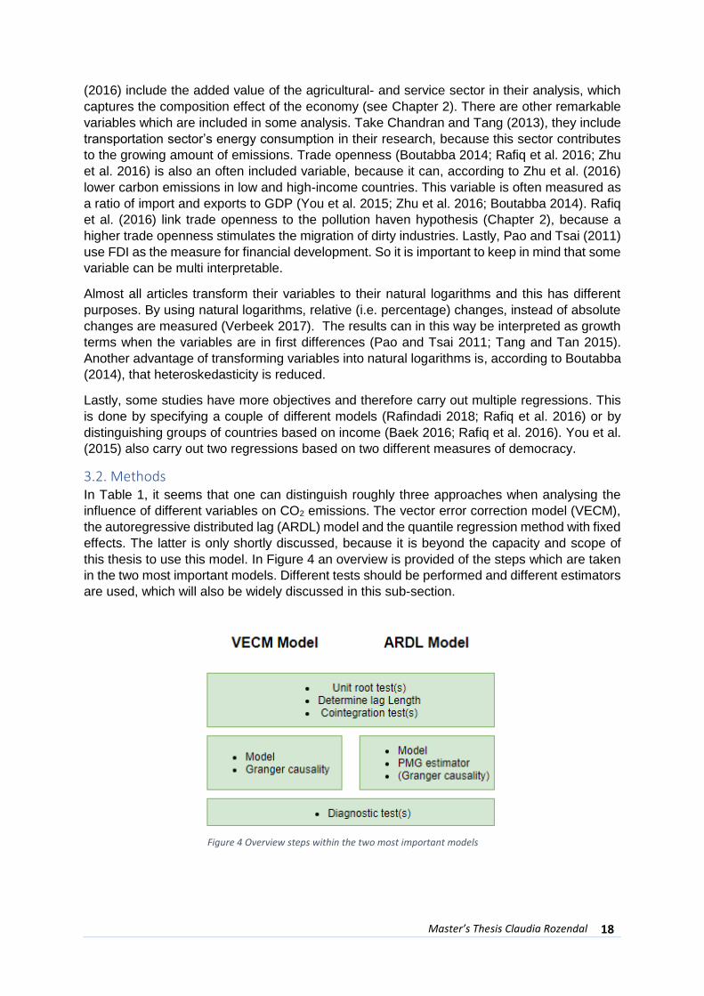
3.2. Methods In Table 1, it seems that one can distinguish roughly three approaches when analysing the

influence of different variables on CO2 emissions. The vector error correction model (VECM),

the autoregressive distributed lag (ARDL) model and the quantile regression method with fixed

effects. The latter is only shortly discussed, because it is beyond the capacity and scope of

this thesis to use this model. In Figure 4 an overview is provided of the steps which are taken

in the two most important models. Different tests should be performed and different estimators

are used, which will also be widely discussed in this sub-section.

Figure 4 Overview steps within the two most important models

Table 1 Literature overview

Article Research question Data retrieved from

Type of data

Variables ** Methods/models/tests Outcomes ***

Omri (2013) Examining the nexus between CO2 emissions, energy consumption and economic growth.

World Bank Panel data of 14 MENA countries, 1990-2011

CO2, energy consumption, GDP*, capital stock, total labour force, total population, financial development, urbanization, trade openness.

Cobb-Douglas production function. Simultaneous-equations models estimated by Generalized Method of Moments (GMM), two-stage least squares (2SLS) and three-stage least squares (3SLS).

Energy consumption ↔ GDP (+) Energy consumption → CO2 (+) GDP ↔ CO2 (+)

You et al. (2015)

Examine whether greater democracy and more financial openness consistently reduce emissions among the most and least emission nations.

World Bank, Marshall and Jaggers (2012), Freedom House (2011), Chinn and Ito (2008)

Panel data of 87 and 97 countries, 1985-2005

CO2, Financial openness, democracy, GDP, population size, trade openness, share of industry, freedom/polity2, Kaopen (financial openness).

Quantile regression method with fixed effect, unit root tests, Wald test.

Democracy → CO2 (+) in lower quantiles and (-) in upper quantiles Population size → CO2 (+) Industrial activity → CO2 (+) in upper quantiles GDP → CO2 (+), Evidence for EKC

Zhu et al. (2016)

Examine the impact of FDI, economic growth and energy consumption on carbon emissions.

World Bank Panel data of the ASEAN-5, 1998-2011

CO2, FDI, GDP*, energy consumption, population size, trade openness, industrial structure, financial development

Quantile regression model with fixed effects, unit root tests, Johansen-Fisher cointegration test, OLS and FMOLS

FDI → CO2 (-) in higher quantiles Energy consumption → CO2 (+) GDP → CO2 (-) in 95th quantile and (+) in lower quantiles Population size → CO2 (+) in lower quantiles and (-) in upper quantiles Trade openness → CO2 (-) No evidence for EKC

Tang and Tan (2015)

Understand the relationship between CO2 emissions, energy consumption, FDI and economic growth.

World Bank, CEIC databases

Time series for Vietnam, 1976-2009

CO2, energy consumption, FDI, GDP*

VECM model, Granger causality, Johansen cointegration test, unit root tests

GDP ↔ CO2 (+) Energy consumption → CO2 (+) FDI ↔ CO2 (-) Evidence for EKC

Pao and Tsai (2011)

What is the impact of both economic growth and financial development on environmental degradation.

World Bank, Energy Information Administration (EIA)

Panel data for BRIC countries, 1980-2007 (1992-2007 for Russia)

CO2, total energy consumption, FDI, GDP*

VECM model, Johansen Fisher test for cointegration, unit root tests, Granger causality, panel cointegration framework

CO2 ↔ FDI (+) GDP → FDI Energy consumption → CO2 (+) GDP ↔ CO2 GDP ↔ energy consumption Energy ↔ FDI Evidence for EKC

Chandran and Tang (2013)

What is the impact of transportation sector's energy consumption, foreign direct investment and income on CO2 emissions.

World Bank Time series data for the ASEAN-5, 1971-2008

Transportation sector's energy consumption, FDI, CO2, GDP*

VECM model, unit root tests, cointegration and Granger causality method

GDP ↔ CO2 (Indonesia and Thailand) GDP → CO2 (Malaysia) Transport energy consumption ↔ CO2 (Thailand and Malaysia) Transport energy consumption ↔ FDI (Thailand and Malaysia) FDI ↔ CO2 (Thailand and Malaysia) No Evidence for EKC

Riti et al. (2017)

What is the impact of energy use and financial development indicators by source in the environment-growth-energy model on CO2 emissions.

World Bank Panel data for 90 countries, 1980-2014

CO2, GDP, population size, renewable energy consumption, fossil fuel energy consumption, financial development indicators

VECM model, CADF and CIPC cointegration tests, DOLS, unit root test, Granger causality

Fossil fuel energy consumption → CO2 (+) GDP → CO2 (+) Renewable energy consumption → CO2 (-) Financial development→ CO2 (-) high and medium-income countries Financial development→ CO2 (+), low-income countries

Boutabba (2014)

Examining the long-run equilibrium and the existence and direction of the causal relationship between carbon emissions, financial development, economic growth,

World Bank Time series data for India, 1971-2008

CO2, financial development, GDP*, energy consumption, trade openness

ARDL approach, unit root tests, Granger causality, dynamic VECM

Financial development → CO2 (+) Financial development → energy use (+) GDP → CO2 (+) Energy consumption ↔ CO2 (+) Evidence for EKC

* Real GDP per capita

**Variables in bold are dependent variables and variables in italic are control variables or less important in the research.

***The arrows indicate if there is a uni- or bidirection relationship. The plus (+) and minus (-) signs indicate a positive or negative relationship respectively.

energy consumption and trade openness.

Rafiq et al. (2016)

What is the impact of sectoral production allocation, energy usage patterns and trade openness on pollutant emissions.

World Bank, Energy Information Administration (EIA)

Panel data of 53 countries, 1980-2010

CO2, trade openness, GDP, non-renewable energy consumption, renewable energy consumption, energy intensity, service sector value added levels, agricultural sector value-added levels, industrialisation total population

ARDL approach, mean group estimators, pooled mean group approaches, dynamic panel models, unit root tests, Johansen Fisher test, Granger causality test

GDP→ CO2 (+) Non-renewable energy consumption → CO2 (+) Energy intensity→ CO2 (+) Service sector→ CO2 (-) Agricultural sector → CO2 (-) Trade liberalisation → CO2 (-) Renewable energy consumption → CO2 (-) Evidence for EKC in high income countries

Baek (2016) What is the effect of FDI inflows, income and energy consumption on CO2 emissions

World Bank, UN conferences on Trade and Development (UNCTAD)

Panel data of the ASEAN-5, 1981-2010

CO2, FDI, GDP*, energy consumption,

ARDL model, pooled mean group (PMG) estimator, Hausman test, unit root tests, cointegration tests

FDI → CO2 (+) GDP → CO2 (+) Energy consumption → CO2 (+) Evidence for EKC

Rafindadi (2018)

Examining the effects of foreign direct investment inflows and energy consumption on environmental pollution

World Bank Panel data for 6 GCC countries, 1990-2014

CO2, energy consumption, FDI, GDP, relative income, domestic investment, energy use

ARDL model, pooled mean group (PMG), dynamic fixed effect (DFE), mean group (MG), unit root test, cointegration test

FDI → CO2 (-) Energy consumption → CO2 (+)

Mert and Bölük (2016)

What is the impact of foreign direct investment and the potential of renewable energy consumption on CO2 emissions

World Bank Panel data for 21 Kyoto countries, 1970-2010

CO2, renewable energy consumption, FDI, fossil fuel energy consumption, income

ARDL approach, unit root, cointegration test, pooled mean group estimator (PMG), Granger causality

FDI→ CO2 (-) Renewable energy consumption→ CO2 (-) No evidence for EKC


3.2.1. Unit root test(s) The first step when applying an econometric method is to look if the data contains a unit root

(see Figure 4). If data contains a unit root (i.e. is non-stationary), that means that the value of

X (in this case) is the same as from the previous period, but with a random error (Dougherty

2016):

𝑋𝑡 = 𝑋𝑡−1 + 휀𝑡

This can cause problems in further analysis. To solve this problem, first differences can be

taken to make the data stationary, the data is then integrated with order one (i.e. I(1)). When

the data is still non-stationary, again differences can be taken, so the data is integrated with

order two (i.e. I(2)) (Dougherty 2016) and so on.

This sub-section discusses what kind of tests for unit roots are applied in the academic articles

used in this chapter. However, first the most general unit root test will be discussed, to get

more insight into the unit root testing procedure. This test is the Dickey-Fuller t-test.

Take this model as an example to illustrate how the test works: 𝑌𝑡 = 𝛽1 + 𝛽2𝑌𝑡−1 + 휀𝑡

H0: β2=1 HA: β2<1

The null-hypothesis is that β2 is one, which means that the data is non-stationary (i.e. contains

a unit root) and the alternative hypothesis is that this parameter is less than one, which means

that the data is stationary.

If the null hypothesis will be rejected, depends on the t-test statistic, which is formulated as

follows:

𝑡 =�̂�2 − 1

𝑠. 𝑒. (�̂�2)

This value should be compared to the critical values. If one wants to do this test for a model

with more lag terms on the right-hand side, the augmented Dickey-Fuller test should be applied

(Dougherty 2016).

After this short explanation of what a unit root test entails, now the many tests which are applied

in the academic articles, will be discussed. A distinction is made between articles which use

time-series data and articles which use panel data.

First, we start with unit root tests applied on time series data. Chandran and Tang (2013) argue

that they use the Dickey-Fuller Generalised Leas Squares (DF-GLS), because of their small

sample size (time-series data for 1971-2008). Also Tang and Tan (2015) adjust their critical

values, because of the small sample size of their study (time-series data for 1976-2009). They

first apply the Augmented Dickey-Fuller (ADF) test and the Kwiatkowski-Phillips-Schmidt-Shin

(KPSS) test. However, for small samples, these tests are not very reliable, because of the so-

called ‘size distortion problem’. Therefore the Monte Carlo simulation based on 100,000

replications is used to generate the critical values for the unit root test, which are more reliable

(Tang and Tan 2015).

Not only small sample sizes can make unit root tests less reliable. If structural breaks occur in

the series, this will bias the results towards non-rejection of the null hypothesis (H0: unit root).

Therefore Boutabba (2014), uses the one- and two-break Lagrange Multiplier (LM) test

statistic. This test is very reliable, because it allows for a break under the alternative and null

hypothesis (Boutabba 2014).


Now we move to articles which applied unit root tests on panel data. First, Pao and Tsai (2011)

distinguish two types of unit root tests. The first category is the test which looks at the common

unit root, that means that there is a common unit root process across the cross-sections (i.e.

the LLC and Breitung test). The other category tests the individual unit root among the cross-

sections (i.e. the IPS, ADF and PP test) (Pao and Tsai 2011). These five tests are widely used

for panel data in the academic literature (Mert and Bölük 2016; Rafindadi 2018; Baek 2016;

Rafiq et al. 2016; Boutabba 2014).

Cross-sectional dependence can cause a bias for the panel unit root tests. Cross-sectional

dependence means that the data across the countries are contemporaneously correlating

(Verbeek 2017). Rafiq et al. (2016) test the existence of cross-sectional dependence with the

test of Friedman, Frees and Pesaran. To minimize this problem, as well as problems

associated with heterogeneity, Riti et al. (2017) apply the cross-sectional-augmented-Dickey

Fuller (CADF) and the cross-sectional Im, Peseran and Shin (CIPS) stationarity tests.

3.2.2. Lag Length Before applying the cointegration test(s), first the lag length of the variables should be chosen.

Multiple tests can be applied: AIC, SBC, FPE, HQ and LR test (Tang and Tan 2015). The first

two, the AIC and Schwarz Bayesian Criterion, are most commonly used in the literature (Riti

et al. 2017; Chandran and Tang 2013; Boutabba 2014; Baek 2016; Rafindadi 2018).

3.2.3. Cointegration test(s) When variables are non-stationary, spurious regressions may occur. This means that two

variables seem to be related, which is not the case (Dougherty 2016). This results in

inconsistent estimators and test statistics. However, this will not be the case, if these non-

stationary variables have a stationary long-run relationship, this is called a cointegration

relationship. So, if variables are I(1) (i.e. integrated with order one), but the linear combination

of these variables is I(0), these variables are cointegrated (Maddala et al. 1998). Thus after

testing for unit roots and determining the optimal lag length, the next step is testing for

cointegration (see Figure 4).

Verbeek (2017) explains cointegration more mathematically; suppose that xt and yt are I(1).

When 𝑦𝑡 − 𝛽𝑥𝑡 (for a certain β) is I(0), that means that there is cointegration. They have a

shared common trend. This means that xt and yt do not drift too far apart in the long run. If

these variables would drift far apart from each other in the long run, this would result in spurious

regression. Granger (1981) also says that cointegration means that “although the two series

may be unequal in the short term, they are tied together in the long run” (Granger 1981 p.129).

If you put it simply, cointegration is the existence of a long-run relationship between the non-

stationary variables (Verbeek 2017). In this sub-section, some cointegration tests will be

discussed. First tests which are applied on time series data and after that the ones commonly

used for panel data.

First, we will have a look at some articles applying cointegration tests on time series data. Tang

and Tan (2015) emphasize that a multivariate cointegration technique should be used instead

of a single-equation approach, because their model has more than two variables and therefore

more than one cointegration relationship can exist (Tang and Tan 2015). The Johansen test

seems to be the most used cointegration test. Chandran and Tang (2013) mention three

important steps when performing the Johansen cointegration test. First, the optimal lag length

should be chosen. Second, the constant and trend (i.e. deterministic components) should be

determined, because the Johansen cointegration test is very sensitive to this choice. And lastly,

there is the concern that, because of the small sample size, there is over-rejection of the null

hypothesis (H0: no cointegration). This issue is solved by adjusting the LR statistic (Chandran

and Tang 2013). The Johansen cointegration test has the advantage that it is not sensitive for


the choice of the dependent variable, because it is assumed that all variables are endogenous

(Tang and Tan 2015). Chandran and Tang (2013) also use the Johansen and the Johansen

and Juselius multivariate cointegration test to see if there is a long-run relationship. This last

test also assumes that all the variables are endogenous and that the test can find more than

one cointegration relationship.

Boutabba (2014) uses a very specific cointegration test; de ARDL F-bounds testing procedure,

which is developed by Pesaran et al. (2001) and can only be applied for time series. In

comparison with Engle and Granger and Johansen and Juselius cointegration techniques, this

testing procedure has a couple of advantages. The variables can be integrated with order one

and/or can be in levels. Next to that, if the research has a small sample, this method has a

higher chance of detection cointegration than the method of Johansen and Juselius. And even

if some independent variables are endogenous, the bounds test still gives unbiased long-run

estimates (Boutabba 2014). Note however that when applying the F-statistic and the variables

are integrated with order two, the test becomes invalid (Boutabba 2014). The F-test has not a

standard distribution and depends on the order of integration of the variables, the number of

explanatory variables in the ARDL model and if there is an intercept and/or time trend included

(Boutabba 2014).

Now we move to panel data cointegration tests. The Johansen Fisher and Kao test seem to

be popular methods to investigate cointegration relationships (Pao and Tsai 2011; Mert and

Bölük 2016). The disadvantage of the Kao cointegration test, however, is that it assumes that

the series in the panel data are homogeneous (i.e. the same). The Pedroni test considers that

the series are heterogeneous across cross-sections (Riti et al. 2017). Another advantage of

the Pedroni test is that it takes into account the cross-sectional dependence, which is already

explained in the previous sub-section (Riti et al. 2017). Therefore Mert and Bölük (2016),

Rafindadi (2018), Riti et al. (2017) and Baek (2016) all use the Pedroni test, which includes

two types of cointegration test: the within dimension test (v-statistic, p-statistics, Philips-Perron

statistic and Augmented Dickey-Fuller statistic), which considers common cross-sectional

autoregressive estimates and between dimension tests (p-statistic, Philips-Perron statistic and

the Augmented Dickey-Fuller statistic) (Riti et al. 2017). When there are mixed results from

these cointegration tests, it is very common to use the error correction term, which should be

negative and less than unity, to prove that there is a cointegration relationship (Baek 2016;

Rafindadi 2018). This error correction term will be further explained in the following sub-

sections.

3.2.4. Vector error correction model (VECM) and autoregressive distributed lag (ARDL) model In the literature, roughly two models can be distinguished (see Figure 4); the vector error

correction model (VECM) and the autoregressive distributed lag (ARDL) model. If there is

cointegration, as discussed in the previous sub-section, short-run dynamics are influences and

therefore an error correction mechanism should be modelled. Both models (can be) adjust(ed)

to a cointegration relationship and (can) include this error correction mechanism. This is the

so-called ‘equilibrium error’ which drives both the short- and long-run relationships in the model

(Verbeek 2017; Blackburne and Frank 2007).

In addition to the error correction mechanism, which can be/is included, the VECM and ARDL

model are both dynamic models. That means that the model captures causal relationships

over more than one period, by including lags (Verbeek 2017). Static models have some

disadvantages and therefore dynamic models are preferred. Rafiq et al. (2016) argue that static

models cannot capture short- and long term relationships, which is possible in dynamic models.

Also, static models assume homogeneity between variables (i.e. are the same) across cross-

sections, which is not realistic in a large sample (Rafiq et al. 2016).


In this sub-section, we therefore discuss these two models: the VECM model and the ARDL

model. Next to that the Granger causality test is used to investigates the direction of the causal

relationships and is often applied in the VECM model approach (see Table 1). Lastly, after the

ARDL model, the Pooled Mean Group (PMG) estimator will be discussed in this sub-section,

because this estimator seems to be the most commonly used estimator for ARDL models.

3.2.4.1. the VECM Model

This sub-section discusses the VECM, which is a model with more than one dependent

variable (captured in a vector) and the inclusion of an error correction term. The latter already

implies that this model assumes that there is cointegration, as explained earlier. The VECM is

discussed in more detail, because in the articles used for this methodology review, all detect

cointegration in their data. However, if there is no cointegration between the variables, a vector

autoregressive (VAR) system should be used, because the one-period error-correction term

(ECT) (which is included to deal with the cointegration relationship) will be removed (Tang and

Tan 2015).

“The vector error-correction model (VECM) is used for correcting disequilibrium in the

cointegration relationship, captured by the ECT, as well as to test for long- and short-run

causality among cointegrated variables” (Pao and Tsai 2001 p.687). Cointegration has

implications for the behaviour of the variables in the short-run. Therefore a mechanism should

be added that drives variables in their long-run equilibrium. This mechanism is represented in

the ECT (Verbeek 2017). So The VECM is a model which is very useful when (a) cointegration

relationship(s) exists and you want to estimate short- and long term parameters (Dougherty

2016). Another feature of the VECM is that all the variables in the VECM model are

endogenous (Dougherty 2016).

The VECM model specified for Pao and Tsai (2011) is as follows and gives an idea of how this

model can look like if the model is used in this thesis:

[ ∆𝑙𝑛𝐶𝑂𝑖𝑡

∆𝑙𝑛𝐸𝑁𝑖𝑡

∆𝑙𝑛𝐹𝐷𝐼𝑖𝑡∆𝑙𝑛𝐺𝐷𝑃𝑖𝑡

∆𝑙𝑛𝐺𝐷𝑃𝑖𝑡2]

=

[ 𝛼1

𝛼2

𝛼3

𝛼4

𝛼5]

+ ∑

[ 𝛽11𝑝 𝛽12𝑝 𝛽13𝑝 𝛽14𝑝 𝛽15𝑝

𝛽21𝑝 𝛽22𝑝 𝛽23𝑝 𝛽24𝑝 𝛽25𝑝



𝛽51𝑝 𝛽52𝑝 𝛽53𝑝 𝛽54𝑝 𝛽55𝑝]

[ ∆𝑙𝑛𝐶𝑂𝑖𝑡−𝑝

∆𝑙𝑛𝐸𝑁𝑖𝑡−𝑝

∆𝑙𝑛𝐹𝐷𝐼𝑖𝑡−𝑝

∆𝑙𝑛𝐺𝐷𝑃𝑖𝑡−𝑝

∆𝑙𝑛𝐺𝐷𝑃𝑖𝑡−𝑝2

]

𝑟𝑝=1 +

[ 𝜃1

𝜃2

𝜃3

𝜃4

𝜃5]

𝐸𝐶𝑇𝑖𝑡−1 +

[ 휀1𝑖𝑡

휀2𝑖𝑡

휀3𝑖𝑡

휀4𝑖𝑡

휀5𝑖𝑡]

(1)

In this example, the vector on the left-hand side includes the dependent variables, among

which the squared GDP to test the existence of the environmental Kuznets curve (see Chapter

2). Whereby i= 1,....,N, are the countries and t= 1,...T is the time period. The error term is

assumed to be serially uncorrelated and the ECTit-1 is the lagged error correction term. The Δ

is the first difference operator, because the data is assumed to be stationary when first

differences are taken. The r is the lag length and Ө is the speed of adjustment (Pao and Tsai

2011). This latter parameter in combination with the lagged error correction term, represents

the long-run equilibrium.

If you write the VECM as separate equations, ECM’s are obtained:

∆𝑙𝑛𝐶𝑂𝑖𝑡 = 𝛼1 + ∑ 𝛽11𝑝∆𝑙𝑛𝐶𝑂𝑖𝑡−𝑝

𝑟

𝑝=1

+ ∑ 𝛽12𝑝∆𝑙𝑛𝐸𝑁𝑖𝑡−𝑝

𝑟

𝑝=1

+ ∑ 𝛽13𝑝∆𝑙𝑛𝐹𝐷𝐼𝑖𝑡−𝑝

𝑟

𝑝=1

+ ∑ 𝛽14𝑝∆𝑙𝑛𝐺𝐷𝑃𝑖𝑡−𝑝

𝑟

𝑝=1

+ ∑ 𝛽15𝑝∆𝑙𝑛𝐺𝐷𝑃𝑖𝑡−𝑝2

𝑟

𝑝=1

+ 𝜃1𝐸𝐶𝑇𝑖𝑡−1 + 휀1𝑖𝑡

….


∆𝑙𝑛𝐺𝐷𝑃𝑖𝑡2 = 𝛼5 + ∑ 𝛽51𝑝∆𝑙𝑛𝐶𝑂𝑖𝑡−𝑝

𝑟

𝑝=1

+ ∑ 𝛽52𝑝∆𝑙𝑛𝐸𝑁𝑖𝑡−𝑝

𝑟

𝑝=1

+ ∑ 𝛽53𝑝∆𝑙𝑛𝐹𝐷𝐼𝑖𝑡−𝑝

𝑟

𝑝=1

+ ∑ 𝛽54𝑝∆𝑙𝑛𝐺𝐷𝑃𝑖𝑡−𝑝

𝑟

𝑝=1

+ ∑ 𝛽55𝑝∆𝑙𝑛𝐺𝐷𝑃𝑖𝑡−𝑝2

𝑟

𝑝=1

+ 𝜃5𝐸𝐶𝑇𝑖𝑡−1 + 휀5𝑖𝑡 (2)

3.2.4.2. Granger causality and estimators

The cointegration test, only tells something about the existence of a long-run causal

relationship. The direction of this relationship can be determined by the (VECM-based)

Granger causality test. Riti et al. (2017) explain Granger causality as follows; “A variable say

‘x’ Granger-causes a variable say ‘y’ if the current values of ‘y’ can be explained by past values

of both ‘x’ and ‘y’ collaboratively” (Riti et al. 2017 p. 890). When the panel cointegration test

shows that there is a long-run cointegration relationship, this means that there must be Granger

causality in at least one direction (Pao and Tsai 2011).

Except for Riti et al. (2017), the other articles who apply a VECM model, do not describe how

the long- and short term parameters are estimated. Riti et al. (2017) determine their long term

parameter estimates by the dynamic ordinary least squares (DOLS) and fully modified ordinary

least squares (FMOLS), which are preferred to OLS, because they are better able to solve the

endogeneity problem and the autocorrelation of the residuals. If there is cross-sectional

dependency among the series, the DOLS estimates are better (Riti et al. 2017).

3.2.4.3. The ARDL Model

The second model, the autoregressive distributed lag model, consists of two different

explanatory variables (i.e. variables on the right-hand side of the model). The lagged values of

the dependent variable are included and also lags of the independent variables are included

in the model (Dougherty 2016). In Sub-section 3.2.2., it is already explained which tests one

should use to find the optimal lag length.

One of the main reasons to use an ARDL model is that rich dynamics can be included and at

the same time the problem of multicollinearity can be reduced (Dougherty 2016). A dynamic

relationship means that there is a causal relationship over more than one period (Verbeek

2017). Or in other words that the model allows for changes in explanatory variables between

periods (ARUP 2010). Also, long- and short-run relationships can be estimated at the same

time with this model (Boutabba 2014).

Another feature of the ARDL model is that consistent estimators can be obtained if the

variables are I(0), I(1) or a combination of both. However, if (some of) the variables are I(2),

the results will produce spurious estimates (Baek 2016; Rafindadi et al. 2018).

The ARDL(p, q1,....qk) model can be specified as follows (Baek 2016; Rafindadi et al. 2018;

Mert and Bölük 2016; Blackburne and Frank 2007):

𝑙𝑛𝐶𝑂𝑖𝑡 = 𝜇𝑖 + ∑ 𝜆𝑖𝑗𝑙𝑛𝐶𝑂𝑖𝑡−𝑗 + ∑ 𝛿′𝑖𝑗𝑋𝑖𝑡−𝑗 + 휀𝑖𝑡𝑞𝑗=0

𝑝𝑗=1 (3)

CO represents, in this case, the amount of CO2 emissions and is the dependent variable. The

X is a vector of all independent variables and their lags.

As explained before an error correction format should be specified (Baek 2016; Mert and Bölük

2016), if a cointegration relationship exists. The ARDL model should be rewritten with an error

correction mechanism (ARUP 2010). Note that, in a single ARDL model, only one cointegration

relationship can exist (Verbeek 2017).


The error correction mechanism can be specified as follows:

𝜑𝑖(𝑙𝑛𝐶𝑂𝑖𝑡−1 − Θ0𝑖 − Θ′𝑖𝑋𝑖𝑡) (4)

With

𝜑𝑖 = −(1 − ∑ 𝜆𝑖𝑗)𝑝𝑗=1 Θ𝑖 = −(∑ 𝛿𝑖𝑗/𝜑𝑖)

𝑞𝑗=0 Θ0𝑖 = −(𝜇𝑖/𝜑𝑖)

This error correction mechanism, consist of the parameter φ, which measures the speed of

adjustment. If this parameter is zero, there is no evidence for cointegration. Between the

brackets is the error correction term, which represents the residuals of the original model (i.e.

the residuals of Equation 3) (Baek 2016; Rafiq et al. 2016). The Θ𝑖 is a vector consisting of the

long-run coefficients for all independent variables.

The error-correction modelling format of the ARDL model is specified as follows (Baek 2016;

Rafindadi et al. 2018; Verbeek 2017; Mert and Bölük 2016; Blackburne and Frank 2007):

∆𝑙𝑛𝐶𝑂𝑖𝑡 = 𝜇𝑖 + 𝜑𝑖(𝑙𝑛𝐶𝑂𝑖𝑡−1 − Θ0𝑖 − Θ′𝑖𝑋𝑖𝑡) + ∑ 𝜆𝑖𝑗

∗ ∆𝑙𝑛𝐶𝑂𝑖𝑡−𝑗 +

𝑝−1

𝑗=1

∑ 𝛿𝑖𝑗′∗∆𝑋𝑖𝑡−𝑗 +

𝑞−1

𝑗=0

휀𝑖𝑡 (5)

With 𝜑𝑖 = −(1 − ∑ 𝜆𝑖𝑗)𝑝𝑗=1 Θ𝑖 = −(∑ 𝛿𝑖𝑗/𝜑𝑖)


𝜆𝑖𝑗∗ = −∑ 𝜆𝑖𝑚

𝑝𝑚=𝑗+1 𝑗 = 1,2, . . . , 𝑝 − 1 𝛿𝑖𝑗

∗ = −∑ 𝛿𝑖𝑚𝑞𝑚=𝑗+1 𝑗 = 1,2, . . . , 𝑞 − 1

One can see that the error correction mechanism (Equation 4) is inserted in the original ARDL

model (Equation 3). The dependent variable and the variables on the right-hand side are also

in first differences, because it is assumed that the variables are non-stationary in levels.

To explain the model a bit further, the p represents the lag length of the dependent variable, q

the lag length of the independent variables and j is the number of time lags. Xit is a vector of k

explanatory variables, whereby 𝜆𝑖𝑗 and 𝛿′𝑖𝑗 are the coefficients for the short-run effects. The

long-run effects are represented in the second term on the right-hand side, the lagged error

correction term. The μi represents the fixed effect of each country and ɛit the error term. The

latter is assumed to be independently distributed across i and t and the regressors Xit, with

means zero and variances larger than zero (Baek 2016; Rafindadi 2018).

3.2.4.4. Estimators

The parameters of the variables should be estimated, and looking at Table 1, roughly two

estimators can be distinguished in the ARDL approach; the Pooled Mean Group (PMG)

estimator and the Mean Group (MG) estimator. These estimators are thus only applied when

the ARDL model is used and when the model is estimated with panel data. Which estimator to

choose, depends on the presence of the homogeneity restriction. This homogeneity restriction

means that the long-run coefficients are the same across the countries (i.e. homogeneous),

but the short-run coefficients and the error variance can vary across the countries (i.e.

heterogeneous) (Mert and Bölük 2016). When this homogeneity restricted is valid, the PMG

estimator should be applied, otherwise the MG estimator should be used. This can be tested

with the Hausman test (Mert and Bölük 2016; Baek 2016; Rafindadi 2018). The Mean group

(MG) estimator assumes full heterogeneity and therefore when applying the MG estimator,

there should be a separate ARDL model for every country (Rafindadi 2018).

All articles use the Pooled Mean Group (PMG) estimator of Pesaran et al. (1999). This

estimator accounts for individual effects. Using the PMG estimator in comparison to fixed


effects estimators has the advantage that parameters of the long-run effects are determined,

while the short-run coefficients, the intercepts and error variances can differ among the

countries (i.e. heterogeneity of the short-run coefficients and the error variance) (Baek 2016).

This estimator also reduces the problem of endogeneity (Rafindadi 2018). Note however that

the PMG cannot be applied when the data is I(2) (Rafindadi 2018).

Rafindadi (2018) applies next to MG and PMG, also the dynamic fixed effects technique (DFE).

Which allows for heterogeneity among the intercepts, but imposes homogeneity on all

coefficients and error variances (Rafindadi 2018).

Rafiq et al. (2016) argue that homogeneity is not realistic and therefore variants of the MG

estimator are used: the augmented mean group (AMG) and the common correlation effects

mean group (CCEMG) estimator. These estimators also have the advantage that they account

for cross-sectional dependence (Rafiq et al. (2016).

3.2.5. Diagnostic test(s) Some articles (both using VECM and ARDL models) apply diagnostic tests after short- and

long-run estimates. Tests are conducted to see if the residuals are normally distributed, if there

is evidence of autoregressive conditional heteroskedasticity (Tang and Tan 2015), or a

specification bias (Riti et al. 2017). The latter two are tested with the Ramsey reset test and

the ARCH test. The Breunsch-Godfrey Lagrangian test looks if there is no autocorrelation (Riti

et al. 2017). Boutabba (2014) checks the stability of the coefficients (i.e. if there are structural

breaks) by the cumulative sum (CUSUM) and the cumulative sum of squares CUSUMSQ

(Boutabba 2014).

3.3. Quantile regression method (with fixed effects) As said before, the quantile regression method (with fixed effects) is beyond the capacities and

scope of this thesis. However, because it seems to be a method which is sometimes used to

research this topic in the literature, the advantages and disadvantages will be shortly discussed

in this sub-section.

One can apply this method if the research question is (also) focused on looking at the

conditional distribution of the dependent variable (You et al. 2015). The parameters are

estimated for different quantiles; from the least emitting countries to the most emitting

countries. By applying the quantile regression method you avoid the problem of biased

outcomes as a result of distributional heterogeneity. Also policymakers are often interested in

the results of the low- and high emitting countries. For high emitting countries, it is more

important to know which variables have a significant influence, because these countries should

prioritize the implementation of policies to tackle environmental pollution. Another advantage

of this method is that it is robust to outliers of the dependent variable and when the error term

is non-normal, this regression is more efficient than an OLS regression (You et al. 2015). The

problem of unobserved individual heterogeneity of countries is corrected by including fixed

effects in the model (Zhu et al. 2016).

You et al. (2015) and Zhu et al. (2016) acknowledge a problem associated with panel quantile

regression with fixed effect. When there is a large number of fixed effects, the incidental

parameters problem can occur and estimates will be inconsistent. Koenker (2004) applies the

so-called shrinkage method to deal with this problem. However, that is the reason this method

is not widely used in scientific research (You et al. 2015; Zhu et al. 2016).


3.4. Outcomes The last column of Table 1, already provides a very clear overview of the outcomes of the

different analysis. In this sub-section, some outcomes are shorty discussed per econometric

approach.

For the articles which use a VECM model, two of them find evidence for the EKC (Tang and

Tan 2015; Pao and Tsai 2011) and one cannot find evidence (Chandran and Tang 2013).

Another contradiction is found between the influence of FDI and emissions. Tang and Tan

(2015) find that FDI can reduce CO2 emissions, while Pao and Tsai (2011) find that it increases

emissions. So there is evidence for both the pollution haven hypothesis and the pollution halo

hypothesis (see Chapter 2). Next to that Tang and Tan (2015) find that the influence of FDI on

CO2 emission is not significant in the short-run. This can be explained by the fact that in the

short term, new production techniques cannot be adapted (i.e. technique effect) (Tang and

Tan 2015). It is also observed that financial development can reduce CO2 emissions in middle-

and high-income countries, while in low-income countries it increases emissions (Riti et al.

2017). Energy consumption has a positive relationship with CO2 emissions (Pao and Tsai

2011; Tang and Tan 2015), however, Riti et al. (2017) distinguish between fossil fuel energy

consumption and renewable energy consumption. The latter has a negative relationship with

the amount of CO2 emissions, which is in accordance with the theory described in Chapter 2.

The articles applying the ARDL approach, all find that GDP increases CO2 emissions, but not

all find evidence for the EKC (Boutabba 2014; Rafiq et al. 2016; Mert and Bölük 2016). There

is also mixed evidence, like in the articles discussed before, on the influence of FDI on CO2

emissions. Baek (2016) argues that FDI increases the amount of CO2 emission, but Rafindadi

(2018) and Mert and Bölük (2016) find a decrease in CO2 emissions. Also energy consumption

is associated with an increase in CO2 emissions. However, renewable energy consumption is

found to decrease the amount of emissions (Rafiq et al. 2016; Mert and Bölük 2016). More

outcomes can be found in Table 1.

For the quantile regression method, the outcomes are as follows. Democracy increases CO2

emissions in the lower quantiles, but decreases emissions in the upper quantiles. Furthermore,

population size, the share of industry and income have a positive relationship with CO2

emissions (You et al. 2015). Zhu et al. (2016) find among others that FDI lowers the amount

of CO2 emissions only in upper quantiles and that economic growth increases emissions only

in lower quantiles. Energy consumption increases emissions in all quantiles (Zhu et al. 2016).

3.5. Data A lot of scientific articles retrieved their data from the Word bank: the World Bank Development

Indicators (You et al. 2015; Zhu et al. 2016; Tang and Tan 2016; Pao and Tsai 2015; Chandran

and Tang 2013; Riti et al. 2017; Boutabba 2014; Rafiq et al. 2016; Baek 201; Rafindadi 2018;

Mert and Bölük 2016). However, some articles use other data sources like the Energy

Information Administration (EIA) (Pao and Tsai 2011; Rafiq et al. 2016) or the UN conferences

on Trade and Development (UNCTAD) (Baek 2016).

3.6. Conclusion In this chapter, an overview is provided of the used methods and tests in the existing literature.

In addition to Table 1, which gives an overview of among others the used variables, methods

and outcomes. The sub-sections discuss in more depth what kind of unit root tests and

cointegration tests there exist and reasons to use these specific type of tests. The VECM and

ARDL model are the most used models in the literature and the models are specified in this

chapter. We see that using the Granger causality test is a logical step after specifying the

VECM model. This test determines the direction of the causality between the variables. Articles


using the ARDL model, often estimate their coefficients with the Pooled Mean Group estimator.

Looking at the outcomes of the articles, it is clear that there are contradicting outcomes and

therefore confirm the relevance of this thesis. After the methodology review in this chapter, the

ARDL model seems to be most suitable to apply in this thesis. Especially because this thesis

focusses on CO2 as the dependent variable and not on the relationship between all variables.

Therefore a single model is suitable to answer the research question. Another advantage of

the ARDL model is that both variables which are (0) and I(1), can be included and still

consistent estimators can be obtained. The ARDL specification can be found below, as well as

the ARDL model with an error correction mechanism. The model will be discussed in more

detail in the next chapter.

ARDL(p,q1,...,qk) model:

𝑙𝑛𝐶𝑂𝑖𝑡 = 𝜇𝑖 + ∑𝜆𝑖𝑗𝑙𝑛𝐶𝑂𝑖𝑡−𝑗 + ∑𝛿′𝑖𝑗𝑋𝑖𝑡−𝑗 + 휀𝑖𝑡

𝑞

𝑗=0

𝑝

𝑗=1

(3)

ARDL(p,q1,...,qk) model with error correction mechanism:



𝑝−1

𝑗=1


𝑞−1

𝑗=0

휀𝑖𝑡 (5)

With 𝜑𝑖 = −(1 − ∑ 𝜆𝑖𝑗)𝑝𝑗=1 Θ𝑖 = −(∑ 𝛿𝑖𝑗/𝜑𝑖)



𝑝𝑚=𝑗+1 𝑗 = 1,2, . . . , 𝑝 − 1 𝛿𝑖𝑗

∗ = −∑ 𝛿𝑖𝑚𝑞𝑚=𝑗+1 𝑗 = 1,2, . . . , 𝑞 − 1


4. Methods and Data

In Chapter 3 an overview is provided of the methodology used in the already existing literature.

From this review, we concluded that the ARDL model seems to fit the objective of this thesis

and will therefore be used to answer the research question: “To what extent do FDI, income

and energy consumption affect the amount of CO2 emissions?”. The tests and steps carried

out in the analysis of this thesis are also largely based on the methodology review of Chapter

3. This chapter will provide in more detail how these tests and other steps will be carried out

and the results will then be discussed in Chapter 5.

An overview of the different steps can be found in Figure 5, below. This chapter starts with

explaining the different unit root tests and the cointegration tests, together with the specific

hypothesis which are tested. After that the ARDL model will be explained and how this model

will be estimated. Which variables are used for the analysis, the countries in the panel and

time period of the analysis will be discussed in detail thereafter. The chapter ends with a short

conclusion.

For the econometric analysis, Stata/IC 15.1 is used. The different steps of the analysis are

largely based on the methodology review of Chapter 3, but are restricted by the options Stata

15.1 is providing.

Figure 5 Graphical overview of the steps in the analysis

4.1. Unit root tests Looking at Figure 5, the first step in the econometric analysis is conducting unit root tests. As

mentioned in Chapter 3, it is important to test for unit roots, because the ARDL model can only

be applied on variables that are stationary in levels or when first differences are taken (i.e. I(0)

and I(1)). However, if the variables contain a unit root, even when first differences are taken,

the estimates will become inconsistent. Also for the next step, testing for cointegration, it is

important to know if variables are integrated with order one (I(1)), because cointegration can

only occur between variables that are I(1).


H0: All panels contain unit roots HA: At least one panel is stationary

First of all, Stata supports six unit root tests, which can be applied on panel data: The Levin-

Lin-Chu test, Harris-Tzavalis test, Breitung test, Im-Pesaran-Shin test, Fisher type tests and

Hadri Lagrange Multiplier stationary test. In Chapter 3, it became clear that five unit root tests

are widely applied for panel data. The LLC and Breitung test (i.e. test for common unit roots

across the cross-sections) and the IPS, ADF and PP test (i.e. test for individual unit root among

the cross-sections). The latter two are part of the Fisher type test in Stata. The tests can take

into account cross-sectional dependence. Cross-sectional dependence can cause problems

for unit root tests and by subtracting the cross-sectional means, this problem is minimized. To

sum up, the following unit root tests will be carried out:

• Levin-Lin-Chu (LLC) test,

• Breitung test,

• Im-Pesaran-Shin (IPS) test,

• Fisher-ADF test,

• Fisher-PP test.

The unit root tests have a slightly different hypothesis that will be tested. The LLC and Breitung

test will test, as explained before, for a common unit root. So their null-hypothesis also states

that the panels contain unit roots. If this hypothesis can be rejected, that means that the panels

are stationary. The same null hypothesis applies to the other three tests, which test for

individual unit roots. However, if this null-hypothesis can be rejected, that means that some

panels are stationary (IPS test) or that at least one panel is stationary (Fisher-ADF and Fisher-

PP).

4.1.1. Lag length

The ARDL model is a dynamic model, which means that the relationship between variables

over more than one period is taken into account. Therefore, the optimal lag length of the

variables, including the dependent variable, should be determined. The optimal lag length will

be obtained by the Akaike Information Criterion (AIC). The LLC and IPS unit root tests,

described above, offer the possibility to obtain the optimal lag length with the AIC and at the

same time perform the unit root tests. The obtained lag lengths are used for both the unit root

tests and the estimation of the ARDL model.

4.2. Cointegration tests When the data is not stationary in levels, but integrated with order one, we will test for

cointegration. This is very important, because cointegration causes problems for the short-run

dynamics in the model. Therefore the model should be adjusted if a cointegration relationship

exists, otherwise inconsistent estimates will be obtained.

Stata supports three cointegration tests: The Kao test, Pedroni test and Westerlund test. As

discussed in Chapter 3, the Kao test has some disadvantages and none of the articles used

for the methodology review applied the Westerlund test. The Pedroni test is however widely

used. Next to the Pedroni test, a cointegration relationship can also be identified by looking at

the error correction term. When the parameter of the error correction term is negative and less

H0: Panels contain unit roots HA: Panels are stationary

H0: All panels contain unit roots HA: Some panels are stationary


than unity, there is evidence for cointegration. This error correction term will be further

explained in the next sub-section.

The Pedroni test includes two different types of tests, as described in Chapter 3: the within

dimension tests (for the whole panel) and between dimensions tests (for the individual

countries). In Stata, the outcomes of the between dimensions tests can be obtained by

including an AR parameter for each individual country. The outcomes of the within dimension

tests can be obtained by including an AR parameter which is the same for the whole panel.

For the cointegration tests, also the cross-sectional means will be subtracted, so the problem

of cross-sectional dependence is reduced.

We will therefore analyse the existence of a cointegration relationship based on:

• The Pedroni test, consisting of:

o Panel v-statistic,

o Panel rho-statistic,

o Panel PP-statistic,

o Panel ADF-statistic,

o Group rho-statistic,

o Group PP-statistic,

o Group ADF-statistic.

• The error correction term.

The ARDL model is a single model and therefore only one cointegration relationship can be

found. Therefore, the null hypothesis and alternative hypothesis of the Pedroni tests state that

there is no cointegration and that all panels are cointegrated, respectively. Stata, however,

only allows testing for cointegration between 7 variables. Which means that not all variables

can be included at the same time. To deal with this problem, we first take out the variables

which are stationary in levels (these can’t be cointegrated), if possible. Next to that, different

groups of variables will be tested for cointegration. For example, first the most important

variables, like CO2, GDP, FDI and energy consumption. When different groups of variables are

tested, we can get an indication of whether a cointegration relationship exists or not. Lastly,

when the outcomes of the Pedroni test show evidence for cointegration, we will include an ECT

in the ARDL model and look if the coefficient shows indeed evidence for cointegration.

4.3. ARDL model After the unit root tests and cointegration tests, the next step is to specify the ARDL model to

estimate de coefficients of the variables. The model is very suitable to investigate how different

variables affect the amount of CO2 emissions in countries. Lagged values of the dependent

variable (CO2 emissions per capita), as well as lagged values of the independent variables,

can be included in the model. Another advantage is that short- and long-run parameters can

be estimated at the same time and that variables can both be I(0) and I(1). Also when there is

cointegration in the data, this problem can be easily solved by inserting an error correction

term (ECT). The model can be estimated in Stata with the pooled mean group (PMG) or mean

group (MG) estimator, which are explained later in this chapter.

The starting point is the long-run relationship we want to investigate in this thesis:

𝑙𝑛𝐶𝑂𝑖𝑡 = 𝛼0+𝛼1𝑙𝑛𝐺𝐷𝑃𝑖𝑡 + 𝛼2𝑙𝑛𝐺𝐷𝑃𝑖𝑡2 + 𝛼3𝑙𝑛𝐹𝐷𝐼𝑖𝑡 + 𝛼4𝑙𝑛𝐹𝐸𝑁𝑖𝑡 + 𝛼5𝑙𝑛𝑅𝐸𝑁𝑖𝑡 + 휀𝑖𝑡 (6)

H0: No cointegration HA: All panels are cointegrated

ECT = negative and less than unity → cointegration ECT≠ negative and less than unity → no cointegration


However, in Chapter 2 and 3, also some other variables seem to be interesting to take into

account in the analysis. Therefore it is interesting to build different models, with different

variables. We start with the variables, included in Equation (6) and specify three more models.

This results in the following long-run relationships:

𝑙𝑛𝐶𝑂𝑖𝑡 = 𝛼0+𝛼1𝑙𝑛𝐺𝐷𝑃𝑖𝑡 + 𝛼2𝑙𝑛𝐺𝐷𝑃𝑖𝑡2 + 𝛼3𝑙𝑛𝐹𝐷𝐼𝑖𝑡 + 𝛼4𝑙𝑛𝐹𝐸𝑁𝑖𝑡 + 𝛼5𝑙𝑛𝑅𝐸𝑁𝑖𝑡+𝛼6𝑙𝑛𝐼𝑁𝐷𝑖𝑡

+ 𝛼7𝑙𝑛𝑆𝐸𝑅𝑉𝑖𝑡 + 휀𝑖𝑡 (7)

𝑙𝑛𝐶𝑂𝑖𝑡 = 𝛼0+𝛼1𝑙𝑛𝐺𝐷𝑃𝑖𝑡 + 𝛼2𝑙𝑛𝐺𝐷𝑃𝑖𝑡2 + 𝛼3𝑙𝑛𝐹𝐷𝐼𝑖𝑡 + 𝛼4𝑙𝑛𝐹𝐸𝑁𝑖𝑡 + 𝛼5𝑙𝑛𝑅𝐸𝑁𝑖𝑡 + 𝛼8𝑙𝑛𝑇𝑅𝐴𝐷𝐸𝑖𝑡

+ 휀𝑖𝑡 (8)

𝑙𝑛𝐶𝑂𝑖𝑡 = 𝛼0+𝛼1𝑙𝑛𝐺𝐷𝑃𝑖𝑡 + 𝛼2𝑙𝑛𝐺𝐷𝑃𝑖𝑡2 + 𝛼3𝑙𝑛𝐹𝐷𝐼𝑖𝑡 + 𝛼4𝑙𝑛𝐹𝐸𝑁𝑖𝑡 + 𝛼5𝑙𝑛𝑅𝐸𝑁𝑖𝑡+𝛼6𝑙𝑛𝐼𝑁𝐷𝑖𝑡

+ 𝛼7𝑙𝑛𝑆𝐸𝑅𝑉𝑖𝑡 + 𝛼8𝑙𝑛𝑇𝑅𝐴𝐷𝐸𝑖𝑡 + 휀𝑖𝑡 (9)

The exact definition of the variables included in the analysis will be explained later in this

chapter. We will now have a look at the specification of the model. In the ARDL model, the

variables on the right-hand side of Equations 6 till 9 (i.e. the independent variables) will be

captured in a 𝐾 × 1 vector. As an example, for the long-run relationship of the first model

(Equation (6)), the following X vector is formulated:

𝑋𝑖𝑡 =

[ 𝑙𝑛𝐺𝐷𝑃𝑖𝑡

𝑙𝑛𝐺𝐷𝑃𝑖𝑡2

𝑙𝑛𝐹𝐷𝐼𝑖𝑡𝑙𝑛𝐹𝐸𝑁𝑖𝑡

𝑙𝑛𝑅𝐸𝑁𝑖𝑡]

(10)

The other three models have an X vector, with their set of independent variables.

The ARDL (p,q1,...,qk) model is used to estimate the long-run relationships, as formulated

above:

𝑙𝑛𝐶𝑂𝑖𝑡 = 𝜇𝑖 + ∑𝜆𝑖𝑗𝑙𝑛𝐶𝑂𝑖𝑡−𝑗 + ∑𝛿′𝑖𝑗𝑋𝑖𝑡−𝑗 + 휀𝑖𝑡

𝑞

𝑗=0

𝑝

𝑗=1

(11)

Keep in mind that this is the general ARDL model and that the four different models that will

be estimated, all have a different X vector. The X vector is included included in the model,

consisting of the (lagged) independent variables, as well as the lagged variable(s) of the

dependent variable: lnCOit-j. The number of lags for the dependent variable and independent

variables are p and q, respectively. The μi is the country-specific intercept and ɛit is the error

term.

This ARDL model should be re-specified if there is cointegration in the data. Cointegration

causes problems in the short-run dynamics and the error correction term (ECT) should be

included, so consistent estimates can be obtained. The error correction term is specified as

follows:

𝜑𝑖(𝑙𝑛𝐶𝑂𝑖𝑡−1 − Θ0𝑖−Θ′𝑖𝑋𝑖𝑡) (12)


With

𝜑𝑖 = −(1 − ∑ 𝜆𝑖𝑗)𝑝𝑗=1 Θ𝑖 = −(∑ 𝛿𝑖𝑗/𝜑𝑖)


The parameter, 𝜑𝑖, measures the speed of adjustment. So if 𝜑𝑖 = 0, there is no evidence for a

long-run relationship (i.e. cointegration). This error correction term consists of this parameter

and the lagged residuals of Equation (11), the term between brackets. The Θ𝑖 is a vector

consisting of the long term coefficients for all independent variables.

The error correction term should be included in the original ARDL model (Equation 11) to obtain

consistent estimates when there is cointegration:

∆𝑙𝑛𝐶𝑂𝑖𝑡 = 𝜇𝑖 + 𝜑𝑖(𝑙𝑛𝐶𝑂𝑖𝑡−1 − Θ0𝑖−Θ′𝑖𝑋𝑖𝑡) + ∑ 𝜆𝑖𝑗

∗ ∆𝑙𝑛𝐶𝑂𝑖𝑡−𝑗 +𝑝−1𝑗=1 ∑ 𝛿𝑖𝑗

′∗∆𝑋𝑖𝑡−𝑗 +𝑞−1𝑗=0 휀𝑖𝑡 (13)

with

𝜑𝑖 = −(1 − ∑ 𝜆𝑖𝑗)𝑝𝑗=1 Θ𝑖 = −(∑ 𝛿𝑖𝑗/𝜑𝑖)



𝑝𝑚=𝑗+1 𝑗 = 1,2, . . . , 𝑝 − 1 𝛿𝑖𝑗

∗ = −∑ 𝛿𝑖𝑚𝑞𝑚=𝑗+1 𝑗 = 1,2, . . . , 𝑞 − 1

This equation also has some other differences, compared with Equation (11). The variables

are now in first differences (i.e. Δ), because cointegration automatically means that the

variables are not stationary in levels. The term between brackets, estimates the long-run

influence of the variables, while the terms with the summation signs, capture the short-run

effects. Note that the number of lags will be p-1 and q-1 in this ARDL model.

4.4. The Hausman test and the (P)MG estimator To estimate the ARDL model, we can choose between two different estimators: the pooled

mean group (PMG) estimator and the mean group (MG) estimator. In Chapter 3, the difference

is already explained. Which one is the most efficient estimator, depends on the validity of the

homogeneity restriction. This homogeneity restriction entails that long-run coefficients are the

same for the whole panel, but short-run coefficients and error variances are country-specific.

This restriction is tested by the Hausman test. Therefore first both estimators should be

performed in Stata, where after the Hausman test concludes which estimator is the most

suitable.

The following null-hypothesis and alternative hypothesis are formulated for the Hausman test:

H0: (b) is consistent, (B) is consistent and efficient or homogeneity restriction is valid

HA: (b) is consistent, (B) is inconsistent

(b)= mg (B)= PMG

The null-hypothesis states that the homogeneity restriction is valid, which means that the PMG

estimator is the most efficient estimator to use. If the null hypothesis can be rejected, the MG

estimator should be used, because the PMG estimator will generate inconsistent results.

4.5. Countries, variables and time period For the analysis, multiple countries and a time period of 25 years is included, which means

that it is a panel analysis. This choice is based on a couple of advantages of panel data. As

explained in Chapter 3, panel data gives more information and greater efficiency in estimation.

Panel data has a larger sample size and the estimators are therefore less sensitive to model

specification. Lastly, by including a country-specific intercept, a model with panel data can


allow for heterogeneity. The countries included in the analysis can be found in Table 2. The

choice of the countries is first of all, based on the availability of the data for the period 1990-

2014. Within this period a selection of countries is made, whereby different income levels and

geographical distribution are taken into account.

Table 2 Countries included in the analysis

Income category Country (Stata code)

Low-income countries Benin (BEN) Senegal (SEN) Togo (TGO) Tanzania (TZA)

Low-medium income countries Ghana (GHA) India (IND) Pakistan (PAK) Philippines (PHL)

Upper-medium income countries Bulgaria (BGR) Mexico (MEX) South Africa (ZAF) Guatemala (GTM)

High-income countries The Netherlands (NLD) New Zealand (NZL) Chile (CHL) Rep. Korea (KOR)

The data is retrieved from the World Bank and the following variables are used in the analysis:

Table 3 Original definitions and units of the variables used for the analysis

Variable Original definition and unit

CO CO2 emissions (metric tons per capita)

GDP GDP per capita (current US$)

FDI Foreign direct investment, net inflows (% of GDP)

REN Renewable energy consumption (% of total final energy consumption)

FEN Fossil fuel energy consumption (% of total)

IND Industry (including construction), value added (% of GDP)

SERV Services, value added (% of GDP)

TRADE Trade (% of GDP)

These variables are chosen, based on the availability of the data, the literature review in

Chapter 2 and the variables included in other research, described in Chapter 3. The research

question of this thesis already indicates that CO2 emissions, GDP, FDI and energy

consumption should be included. Whereby the latter is split up in renewable energy

consumption and fossil fuel energy consumption, to see if there is a difference in the influence

of the two different sources of energy. In Chapter 2, also other variables are mentioned as

relevant in such an analysis. The two other variables, IND and SERV, represent the amount

of GDP generated by the industry- and the service sector, respectively. These variables

represent the composition effect. This effect postulates that an industry-based economy emits

more CO2 emissions, than a service-oriented economy. Therefore these variables are included

to investigate the strength of this effect. Lastly, from Chapter 2 it became clear that a lot of

articles include variables like trade(openness) and financial development/openness in their

analysis. A trade variable can be added in a model to avoid omitted variable bias, but another

argument is that more trade can also accelerate economic growth, which has an effect on the

amount of CO2 emissions. Therefore, the last variable in the analysis captures the amount of

trade in a country as a percentage of GDP.

All variables will be transformed into natural logarithms, because in that way, the parameters

can be interpreted as relative (i.e. percentage) changes. Expressing the variables in relative


numbers can also reduce heteroskedasticity. This, however, causes problems for the FDI

variable, because natural logarithms can only be taken from positive numbers, which is not

always the case for FDI. Therefore we add a constant (+10) to the variable, like Baek (2016)

did in his research. Also a new variable is created, the squared GDP (GDP2), to test the

environmental Kuznets curve (EKC) (see Chapter 2).

4.5.1. Descriptive statistics In Table 4, a summary of the variables can be found for the 16 countries. For every variable,

we have 400 observations, because we have data over a time period of 25 years for 16

countries. The diversity of the countries is very clear when looking at especially the minimum

and maximum values of variables. If we look at TRADE for example, the minimum is 15

percent, while the maximum is 150 percent trade of the amount of GDP. That the minimum

value and the maximum value are far apart from each other, is the case of every variable.

However, remarkable are the values of FDI. The minimum and maximum value are far apart

from each other, but the mean has a low value, as well as the standard deviation. That would

imply that this variable has some strong upwards outliers.

Table 4 Descriptive statistics

Variable Mean Std. Dev. Min Max Observations

CO 3.501 3.773 0.078 11.967 400

GDP 6697.139 10982.79 157.061 57644.48 400

FDI 3.334 6.765 -5.007 86.611 400

REN 40.773 28.076 0.442 95.178 400

FEN 57.191 26.680 3.781 98.045 400

IND 25.768 6.393 11.983 51.275 400

SERV 50.977 9.341 26.246 69.910 400

TRADE 64.754 25.483 15.506 150.054 400

4.6. Conclusion This chapter describes which steps are carried out in this research. Five unit root tests are

applied, to see if the data is stationary in levels or first differences. When it turns out that (some

of) the variables are I(1), also cointegration should be tested. The Pedroni test includes 7

different cointegration tests, which should be carried out. Next to that, we will have a look at

the ECT, to see if cointegration is a problem in the data. The four different ARDL models are

specified and the variables which are used. All variables are transformed into natural

logarithms, so relative changes instead of absolute changes will be obtained. The model can

be estimated with the PMG or MG estimator. Which estimator is the most suitable, will be

tested with the Hausman test. The analysis will include a panel of 16 countries over the period

of 1990 till 2014. This decision is based on the availability of the data and a representation of

a variety of countries. The results of the tests and the model estimations will be widely

discussed in the next chapter.


5. Results

The previous chapter discussed, which steps will be carried out in the econometric analysis of

this thesis. These steps were based on Chapter 3, which described elaborately how other

studies performed a similar analysis. In this chapter, the results of the tests and model

estimation will be discussed. Whereby the concepts and theories explained in Chapter 2, will

be linked to the outcomes of the model. Therefore this chapter will answer the research

question of this thesis: To what extent do FDI, income and energy consumption affect the

amount of CO2 emissions? First, the outcomes of the unit root tests, the determination of the

lag length and the cointegration test results will be discussed. Based on these outcomes, the

final model is specified and thereafter, the outcomes of the four models will be presented. At

the end of the chapter an overall conclusion is provided.

Two important concepts will be used throughout the chapter and it is therefore important to

explain them beforehand: statistical significance level and p-values. For every test that is

conducted and every parameter that is estimated, a test statistic and a corresponding p-value

are generated. With this p-value, we can conclude if the null-hypothesis of the test can be

rejected or not (i.e. if the alternative hypothesis can be accepted). One should specify a value

for the level of significance (also referred to as α), which is most times 0.05. If the p-value is

lower than α, the null hypothesis is rejected and if the p-value is higher than the significance

level, the null hypothesis is not rejected. The hypothesis of the unit root-, cointegration- and

Hausman test are already explained in the previous chapter. However, when the coefficients

of the variables are determined with the PMG and MG estimator, the null hypothesis is as

follows. We test if the coefficient of the parameter is different from zero (H0: coefficient = 0). If

the p-value is lower than the significance level, the null hypothesis can be rejected and proves

that the variable has a significant influence on the dependent variable (Ott et al. 2010).

5.1. Unit root tests The unit root tests, test for the existence of a unit root in de data and thus if the data is

stationary. The ARDL model can be estimated with both I(0) and/or I(1) variables. It is thus

important that the variables are stationary in levels or when first differences are taken (i.e. I(1)).

In Table 5, the outcomes of the five different unit root tests can be found. Some variables

contain a unit root in levels, but are clearly stationary in first differences. Look at lnCO for

example, all tests show that there is strong evidence for a unit root, but in first differences, the

null hypothesis that the data contains a unit root, can be rejected at a 1 percent significance

level. This is also the case for lnREN and lnTRADE. The outcomes are sometimes also

ambiguous, when some tests reject the null hypothesis of the presence of a unit root and others

show evidence that some/at least one panel(s) is/are stationary. Looking at for example

lnGDP2, the tests give different results. Therefore, first differences are taken, whereafter all

the tests reject the null hypothesis with a significance level of 1 percent. lnFDI is the only

variable where, without any doubt, the data is stationary in levels. The tests all reject the null

hypothesis with a 1 percent significance level. As emphasized by Baek (2016), the ARDL

model is suitable for both variables which are stationary in levels and in first differences. The

conclusion of the unit root test is therefore that all variables can be used to estimate the ARDL

model and that cointegration should be tested because most variables are I(1).


The asterisks ***, ** and *, indicate a statistical significance at a 1, 5 and 10 percent level, respectively. The values between brackets ( )

denote the p-values.

Table 5 Outcomes unit root tests

5.2. Lag length The optimal lag length is determined with the Akaike Information Criterion (AIC), which is

carried out in the LLC and IPS unit root tests. The optimal lag lengths can be found in Table 6,

whereby the second column shows the results of the AIC. For the other unit root tests, also lag

lengths are taken into account, whereby the lag lengths are rounded, as shown in column 3 of

the table. For the ARDL model with an error correction term, the lag lengths minus one should

be used, which result in the lag lengths in the last column of Table 6.

Table 6 Outcomes optimal lag length

Variable Lag length determined by AIC

Lag Length used for unit root testing

Lag Length used for the ARDL model with ECT

lnCO 1.81 2 1

lnGDP 1.38 1 0

lnGDP2 1.5 1 0

lnFDI 1.13 1 0

lnREN 0.75 1 0

lnFEN 2.13 2 1

lnIND 1.56 2 1

lnSERV 0.25 0 0

lnTRADE 1 1 0

5.3. Cointegration tests The Pedroni cointegration test is applied, because a lot of variables are I(1) and therefore

cointegration can be a problem. The Pedroni test, consist of four panel specific cointegration

tests and three groups specific tests. Stata limits the number of variables that can be tested to

a maximum of seven, through which we specified different groups of variables, to test for

cointegration:

• Group 1: lnCO, lnGDP, lnGDP2, lnREN, lnFEN

• Group 2: lnCO, lnGDP, lnGDP2, lnREN, lnFEN, lnIND, lnSERV

• Group 3: lnCO, lnGDP, lnGDP2, lnREN, lnFEN, lnTRADE

Variable

levels First differences

LLC Breitung IPS ADF PP LLC Breitung IPS ADF PP

lnCO 0.03 (0.51)

2.07 (0.98)

-1.21 (0.11)

1.86 (0.97)

1.33 (0.91)

-13.71*** (0.00)

-3.29*** (0.00)

-13.11*** (0.00)

-4.89*** (0.00)

-16.53*** (0.00)

lnGDP -8.07**

(0.02) -1.04 (0.15)

-2.59*** (0.00)

-1.82** (0.03)

-2.36** (0.01)

-11.20*** (0.00)

-6.02*** (0.00)

-12.52*** (0.00)

-11.11*** (0.00)

-16.29*** (0.00)

lnGDP2 -3.21*** (0.00)

-0.73 (0.23)

-1.90** (0.03)

-1.23 (0.11)

-1.45* (0.07)

-11.78*** (0.00)

-6.64*** (0.00)

-12.29*** (0.00)

-10.85*** (0.00)

-15.72*** (0.00)

lnFDI -4.90*** (0.00)

-3.97*** (0.00)

-4.64*** (0.00)

-4.01*** (0.00)

-5.06*** (0.00)

lnREN 2.69 (1.00)

4.18 (1.00)

4.53 (1.00)

4.02 (1.00)

4.16 (1.00)

12.27*** (0.00)

-5.76*** (0.00)

-12.40*** (0.00)

-8.62*** (0.00)

-15.49*** (0.00)

lnFEN -9.01*** (0.00)

1.63 (0.95)

-5.52*** (0.00)

-2.30** (0.01)

1.48 (0.93)

-9.59*** (0.00)

-4.52*** (0.00)

-10.99*** (0.00)

-10.15*** (0.00)

-14.68*** (0.00)

lnIND -1.71** (0.04)

-0.70 (0.24)

-1.75** (0.04)

-1.67* (0.05)

-1.03 (0.15)

-13.50*** (0.00)

-1.52* (0.07)

-12.81*** (0.00)

-6.19*** (0.00)

-16.07*** (0.00)

lnSERV -3.31*** (0.00)

-1.62* (0.05)

-2.80*** (0.00)

-2.53** (0.01)

-2.53** (0.01)

-12.96*** (0.00)

-11.53*** (0.00)

-13.18*** (0.00)

-16.28*** (0.00)

-16.28*** (0.00)

lnTRADE -0.94 (0.17)

-1.43* (0.08)

-0.59 (0.28)

-0.98 (0.16)

-0.71 (0.24)

-12.37*** (0.00)

-5.56*** (0.00)

-12.85*** (0.00)

-9.42*** (0.00)

-14.68*** (0.00)


The asterisks ***, ** and *, indicate a statistical significance at a 1, 5 and 10 percent level,

respectively. The values between brackets ( ) denote the p-values.

The FDI variable is not included in any of the tests, because this variable is I(0) and can

therefore not be cointegrated. The groups are based on the four models that are already shorty

discussed in the previous chapter. The first group includes the most important variables (tested

in Model 1) and the other two groups include the extra variables included in Model 2 and 3,

respectively.

In Table 7, the outcomes of the Pedroni test can be found. It is clear that, irrespective of the

group of variables, the outcomes of the test are ambiguous. For group 1, four tests cannot

reject the null hypothesis of no cointegration and three can reject the null hypothesis, with a

significance level of 5% (or less). The second group shows more evidence for cointegration,

whereby five tests accept the alternative hypothesis of cointegration. The last group has four

tests with a p-value lower than 0.05, and therefore accept the alternative hypothesis. In

conclusion, we can say that the results of the cointegration tests are ambiguous and therefore

an ECT will be included. If this ECT is negative and less than unity, this will prove the existence

of cointegration.

Table 7 Outcomes cointegration tests

Cointegration test Group 1 Group 2 Group 3

Panel v-statistic -2.45** (0.01)

-3.48*** (0.00)

-2.97*** (0.00)

Panel rho-statistic 1.84** (0.03)

2.78*** (0.00)

2.40** (0.01)

Panel PP-statistic 0.06 (0.48)

-0.43 (0.34)

-0.11 (0.45)

Panel ADF-statistic -0.26 (0.40)

-0.99 (0.16)

-0.79 (0.21)

Group rho-statistic 2.75*** (0.00)

3.84*** (0.00)

3.04*** (0.00)

Group PP-statistic -0.28 (0.39)

-1.40* (0.08)

-1.02 (0.15)

Group ADF-statistic -0.52 (0.30)

-1.62* (0.05)

-2.18** (0.01)

5.4. Model specification The lag length has been determined and the Pedroni test indicates a possible cointegration

relationship between the variables, now the ARDL models with ECT can be formulated.

In Chapter 4, four different models are formulated. The first model is the one with the most

important variables, according to the literature described in Chapter 2. After that, we formulate

model 2 and 3, whereby the most important variables are included and 2 more variables and

1 more variable, respectively. The fourth model includes all 9 variables.

The general ARDL (p,q1,....,qk) model with ECT is formulated as follows:



𝑝−1

𝑗=1


𝑞−1

𝑗=0

휀𝑖𝑡 (14)

with

𝜑𝑖 = −(1 − ∑ 𝜆𝑖𝑗)𝑝𝑗=1 Θ𝑖 = −(∑ 𝛿𝑖𝑗/𝜑𝑖)

𝑞𝑗 Θ0𝑖 = −(𝜇𝑖/𝜑𝑖)


𝑝𝑚=𝑗+1 𝑗 = 1,2, . . . , 𝑝 − 1 𝛿𝑖𝑗

∗ = −∑ 𝛿𝑖𝑚𝑞𝑚=𝑗+1 𝑗 = 1,2, . . . , 𝑞 − 1


The only difference between the models is the X vector, consisting of all the independent

variables, and the corresponding lag lengths (see last column Table 6). Below, the 4 different

X vectors for the models are formulated.

Model 1: ARDL (1,0,0,0,0,1) model, with X vector:

𝑋𝑖𝑡 =



𝑙𝑛𝐹𝐷𝐼𝑖𝑡𝑙𝑛𝑅𝐸𝑁𝑖𝑡

𝑙𝑛𝐹𝐸𝑁𝑖𝑡]

(15)

Model 2: ARDL (1,0,0,0,0,1,1,0) model, with X vector:

𝑋𝑖𝑡 =




𝑙𝑛𝐹𝐸𝑁𝑖𝑡

𝑙𝑛𝐼𝑁𝐷𝑖𝑡

𝑙𝑛𝑆𝐸𝑅𝑉𝑖𝑡]

(16)

Model 3: ARDL (1,0,0,0,0,1,0) model, with X vector:

𝑋𝑖𝑡 =

[

𝑙𝑛𝐺𝐷𝑃𝑖𝑡




𝑙𝑛𝑇𝑅𝐴𝐷𝐸𝑖𝑡]

(17)

Model 4: ARDL (1,0,0,0,0,1,1,0,0) model, with X vector:

𝑋𝑖𝑡 =

[

𝑙𝑛𝐺𝐷𝑃𝑖𝑡




𝑙𝑛𝐼𝑁𝐷𝑖𝑡

𝑙𝑛𝑆𝐸𝑅𝑉𝑖𝑡

𝑙𝑛𝑇𝑅𝐴𝐷𝐸𝑖𝑡]

(18)

5.5. Model estimation The models are estimated with both the mean group (MG) estimator as well as the pooled

mean group estimator (PMG). Thereafter the Hausman test is applied, to see which of the two

estimators is efficient. All four models and their results will be discussed in this sub-section.

5.5.1. Model 1 The results of the first model can be found in Table 8 below. We will first look at the result of

the Hausman test. The chi-square statistic has a value of 0.54 with a corresponding p-value of

0.99. This means that the null hypothesis can’t be rejected. That means that the homogeneity

restriction is valid and the results of the PMG estimator the most efficient. Therefore, we focus

on the results of the PMG estimator. First, the ECT is statistically significant (with a significance


The asterisks ***, ** and *, indicate a statistical significance at a 1, 5 and 10 percent level, respectively. The values between

brackets ( ) denote the p-values.

level of 0.05) and the coefficient has a value of -0.14, which indicates that the model indeed

contains a cointegration relationship. The first remarkable outcome is that in the long-run, only

one variable has a significant influence on the amount of CO2 emissions per capita. The

variable of fossil fuel energy consumption has a coefficient of 0.92, which is statistically

significant at a 1 percent significance level. This is in line with Chapter 2, were (fossil fuel)

energy consumption is associated with an increase in CO2 emissions. A one percent increase

in fossil fuel energy consumption as a percentage of the total amount of energy consumption,

means that there is 0.92 percent increase in CO2 emissions per capita. In the short run, only

renewable- and fossil fuel energy consumption have a significant influence on the amount of

CO2 emissions per capita. Whereby fossil fuel energy consumption increases the amount of

CO2 emissions and renewable energy decreases emissions. The latter is also in line with the

expectations, as explained in Chapter 2.

Table 8 Outcomes Model 1

Variables Pooled mean group Mean group

Long-run Short-run Long-run Short-run

ECT -0.14**

(0.02) -0.85***

(0.00)

LnCOit-1 -0.10 (0.18)

0.13 (0.12)

lnGDPit -0.16 (0.81)

1.48 (0.12)

-0.75 (0.69)

1.34 (0.30)

lnGDP2it 0.05 (0.29)

-0.11 (0.13)

0.12 (0.36)

-0.11 (0.25)

lnFDIit -0.15 (0.17)

0.00 (0.98)

-0.08 (0.62)

0.04 (0.40)

lnRENit 0.35 (0.14)

-0.45*

(0.06) 0.12 (0.82)

-0.02 (0.91)

lnFENit 0.92***

(0.00) 0.82**

(0.01) 0.56 (0.45)

0.61*

(0.05)

lnFENit-1 0.17 (0.45)

0.09 (0.63)

Constant -0.86**

(0.02) 5.49

(0.43)

Hausman 0.54 (0.99)

5.5.2. Model 2 In Model 2, the composition effect is taken into account. Next to the most important variables

(Model 1), the two variables for the percentage that the industry sector and service sector add

to the total amount of GDP, are added to the model. The Hausman test, again shows that the

PMG estimator is the most efficient, with a p-value of 0.98. We also see that the ECT is

negative and less than unity, so this proves a cointegration relationship. Now the two extra

variables are added, GDP per capita and renewable energy consumption show a statistically

significant influence on the amount of CO2 emissions per capita, while they were not significant

in the previous model. Starting with the long-run effect of the variables, we see that GDP per

capita has a positive relationship with CO2 emissions per capita (i.e. increases the amount of

emissions). This is in line with the scale effect, discussed in Chapter 2. We therefore can

conclude that the scale effect cannot be outweighed by for example the technique effect. The

fossil fuel energy consumption variable and the renewable energy consumption variable have,

as expected, a positive and negative effect on the amount of emissions per capita, respectively.

The other variable, which is significant in the long run, is the share of industry as a percentage

of GDP. One expects that, the more industry in a country, the more emissions per capita, in

accordance with the composition effect. However, the estimation shows that when the amount




of industry increases by 1 percent, emissions per capita will fall with 0.56 percent. This

outcome is statistically significant at a 1 percent level and is in contradiction with what is

expected. Possibly, the industry sector is not as polluting as one would expect. In the short

run, only fossil fuel energy consumption has a positive influence on the amount of CO2

emissions per capita.




ECT -0.22***

(0.00) -1.04***

(0.00)

lnCOit-1 -0.08 (0.25)

0.28**

(0.02)

lnGDPit 0.40**

(0.01) -0.26 (0.80)

-1.90 (0.61)

1.21 (0.63)

lnGDP2it -0.01 (0.28)

0.02 (0.83)

0.27 (0.29)

-0.12 (0.52)

lnFDIit 0.01 (0.90)

-0.02 (0.70)

-0.30 (0.30)

0.06 (0.40)

lnRENit -0.23***

(0.00) -0.29 (0.39)

1.51 (0.23)

0.15 (0.78)

lnFENit 1.06***

(0.00) 0.55**

(0.03) 0.55 (0.69)

0.61 (0.18)

lnFENit-1 0.06 (0.83)

0.05 (0.84)

LnINDit -0.56***

(0.00) -0.12 (0.33)

-0.98 (0.50)

-0.86 (0.10)

LnINDit-1 0.04 (0.65)

-0.28 (0.17)

lnSERVit 0.03 (0.76)

-0.51 (0.12)

-3.28**

(0.02) -1.14 (0.14)

Constant -0.80***

(0.00) 18.48

(0.23)

Hausman 1.48 (0.98)

5.5.3. Model 3 The third model adds trade as a percentage of GDP, as an extra variable on top of the variables

in Model 1. Again, the null hypothesis of the Hausman test cannot be rejected, that means that

the PMG is the most efficient estimator. Also the ECT is negative and less than unity, which

indicates the existence of cointegration. In Table 10, the results can be found and what stands

out immediately is that in the long-run, all variables have a significant influence on CO2

emissions per capita. Starting with the variables of GDP. The outcomes are as expected when

looking at the EKC. The EKC postulates an inverted U-shape, which implies that the variable

for GDP per capita should be positive and GDP2 per capita negative. This is indeed the case,

as the coefficients are 1.34 and -0.07, respectively. The energy consumption coefficients are,

again, as expected positive (for fossil fuel energy consumption) and negative (for renewable

energy consumption). If we compare the results with the previous model, the coefficient of

renwable energy consumption is almost the same, while the coefficient of fossil fuel energy

consumption is more than three times smaller than in Model 2. As discussed in Chapter 2,

there was no clear answer about the influence of FDI on environmental pollution as well as the

influence of the amount of trade. In Table 10, we see that FDI has a small negative effect on

the amount of CO2 emissions per capita and trade has a small positive effect on the amount

of CO2 emissions per capita. The latter also confirm that trade, as a variable, should be

included in such an analysis, because it shows an influence on environmental pollution. This




was doubtful, because only a few articles included trade as an important variable. Lastly, in

the short run, only fossil fuel energy consumption has a positive and significant influence on

the amount of CO2 emissions per capita.




ECT -0.34**

(0.01) -0.81***

(0.00)

LnCOit-1 -0.00 (0.97)

0.12 (0.23)

lnGDPit 1.34***

(0.00) -0.03 (0.97)

-30.22 (0.33)

2.33 (0.13)

lnGDP2it -0.07***

(0.00) -0.01 (0.93)

2.43 (0.32)

-0.18 (0.12)

lnFDIit -0.03**

(0.02) -0.03 (0.50)

2.72 (0.33)

-0.02 (0.71)

lnRENit -0.22***

(0.00)

-0.30

(0.22)

7.68

(0.32)

0.02

(0.95)

lnFENit 0.29**

(0.01) 0.69**

(0.01) -0.82 (0.56)

0.51**

(0.03)

lnFENit-1 0.06 (0.79)

-0.06 (0.79)

lnTRADEit 0.09**

(0.01)

0.06

(0.24)

4.39

(0.30)

0.10

(0.15)

Constant -2.03***

(0.00) -2.22

(0.69)

Hausman 2.07 (0.91)

5.5.4. Model 4 The estimation of Model 4 will show the results of all the variables discussed so far in the

previous models (see Table 11). Some results are the same as seen in the previous models

and others will give opposite results. Again, the Hausman test indicates that the PMG estimator

is the most efficient and also the ECT has a coefficient that is negative and less than unity,

which means that there is indeed cointegration. Again, the GDP per capita and GDP2 per capita

show evidence for the EKC, because the coefficient of the former is positive and of the latter

negative. FDI has a negative impact on CO2 emissions per capita, but in this model, the effect

is stronger (-0.20) in comparison to the previous model (-0.03). Remarkable is that renewable

energy consumption seems to have a positive influence on CO2 emissions per capita, which

is not in line with the previous results and the expectations described in Chapter 2. However,

if you look at the short-run effect, the coefficient is negative, as expected. Also the variables

that take into account the share of GDP from the industry and service sector show remarkable

results. One would expect that the higher the share of industry, the more CO2 emissions and

that the service sector is less polluting, so this coefficient would be negative. However, looking

at the outcomes in Table 11, the higher the share of the industry sector, the lower the emissions

per capita and the higher the share of the service sector, the higher the emissions per capita.

Lastly, trade has both in the long and short-run a significant effect on the amount of emissions.

In the short run, more trade results in more emissions per capita, while in the long-run it will

lower the amount of emissions per capita in a country. The latter can indicate that the technique

effect will prevail, because more trade can diffuse cleaner and more efficient production

techniques which can reduce the amount of CO2 emissions. It takes time to implement new

and cleaner techniques, which will explain the positive effect in the short-run and the negative

effect in the long-run.







ECT -0.20***

(0.00) -0.88**

(0.01)

lnCOit-1 -0.13 (0.10)

0.20 (0.21)

lnGDPit 1.73***

(0.00)

-0.03

(0.99)

2.06

(0.77)

1.88

(0.63)

lnGDP2it -0.09***

(0.00) -0.01 (0.90)

-0.02 (0.97)

-0.18 (0.53)

lnFDIit -0.20***

(0.00) -0.03 (0.62)

0.35 (0.52)

0.07 (0.76)

lnRENit 0.14**

(0.03) -0.43*

(0.05) 6.92 (0.26)

-0.26 (0.80)

lnFENit 0.75***

(0.00) 0.58**

(0.03) 4.19 (0.12)

0.27 (0.74)

lnFENit-1 0.16 (0.57)

-0.15 (0.71)

LnINDit -0.14*

(0.09) -0.19 (0.15)

0.07 (0.97)

-1.09 (0.16)

LnINDit-1 0.05 (0.48)

-0.60 (0.07)

lnSERVit 0.22***

(0.00) -0.34 (0.26)

-4.06**

(0.04) -0.95 (0.31)

LnTRADEit -0.30***

(0.00) 0.15**

(0.01) -0.25 (0.49)

-0.02 (0.88)

Constant -1.96***

(0.00) 24.16

(0.32)

Hausman 0.35 (1.00)

5.6. High- and low-income countries The above analysis is done for a panel of 16 countries, with a wide range in the level of income between the countries. The conclusions, which are given above are therefore very general. As mentioned in Chapter 2, the effects of variables on the amount of CO2 emissions depends sometimes on the ‘phase’ of the country. For example, if countries have a low income level, FDI will have a different impact than FDI in countries with a high income level. This refers to the pollution haven hypothesis, which is discussed elaborately in Chapter 2. This pollution haven hypothesis postulates that high-income countries reallocate their polluting production to low-income countries. Searching for evidence for this hypothesis is more difficult in an analysis as done in this chapter. That’s because, in this analysis, we cannot distinguish between high and low-income countries. Also the other variables included in the analysis will show probably other results when we make a panel of high-income countries and low-income countries. For this thesis, the panel of 16 countries was split up in two panels: the low- and medium-low income countries and the upper-medium and high-income countries. The next step was to carry out the analysis for these two new panels, with the corresponding unit root tests, cointegration test and the estimation of the four models. However, the results of the models were not as expected. For simplicity, we will call the panel with the low-income countries, panel B1 and the panel with high-income countries, panel B2. For the former, only Model 1 and model 3 showed consistent results. Panel B2 only showed ‘normal’ results for Model 2 and 4 (see Table 12). First of all, it is surprising that the two panels, both estimate 2 models in the right way, but not the same models. That is remarkable, but also raises the question of why not all the models can be estimated. Therefore, we will explain what went wrong in estimating model 2 and 4 in panel B1 and in estimating model 1 and 3 in panel B2.


Table 12 Overview, model estimation for two different panels

Panel B1 Panel B2

Model 1 ✓ Problems Hausman test

Model 2 ✓

Model 3 ✓ ECT not significant

Model 4 Problems Hausman test ✓

In Table 12, a clear overview is provided of the models that can be estimated and of the problems encountered by estimating the other models. No results can be obtained for Model 2 of panel B1. The remaining models can be estimated, but give uncommon results. The problem occurring in model 4 of panel B1 and model 1 of panel B2 is related to the Hausman test. The chi-square statistic is negative, which is not allowed in this test statistic. Therefore, the p-value for the Hausman test is not generated and it can not be determined which estimator is consistent and efficient. For model 3 of panel B2, the problem that occurs is that the Hausman test points to the PMG estimator as the most efficient estimator. However, the ECT is not significant, which means that there is no cointegration. We discussed in Chapter 4, that the general ARDL model can be applied in that case. However, the PMG estimator or MG estimator are not suitable for estimating a general ARDL model. Applying another estimator for this model is beyond the scope and time of this thesis. In conclusion, the results of the models for two separate panels give some problems for the Hausman test and also an explanation why Models 1 and 3 for panel B1 and Models 2 and 4 for panel B2, can be estimated without such problems is not clear. A solution, to distinguish between the 8 low- and 8 high-income countries is to include a dummy variable in the original analysis. Unfortunately, a dummy variable cannot be added when the model is estimated with the PMG and MG estimator in Stata. It is difficult to give an explanation, why the models can be estimated for the panel of 16 countries, but not when we split up this panel into 8 countries per panel. The only explanation, which is obvious, would be that the estimator is developed for a large N and a large T (Blackburne and Frank 2007). By splitting up the original panel, maybe the number of countries is too small. However, when looking at Table 1 in Chapter 3, we see that Baek (2016) and Rafindadi et al. (2018) apply the PMG and MG on a panel with five and six countries, respectively. In conclusion, it is decided to omit the analysis for the 2 separate panels from this thesis.

5.7. Conclusion This chapter shows the results of the econometric analysis. First, all the variables are tested

for unit roots and all the variables are stationary in levels or first differences. Secondly, the

optimal lag lengths for both the dependent and the independent variables are determined with

the Akaike information criterion. Thereafter, the Pedroni test is carried out, to see if there is

cointegration in the data. This test was carried out, because most of the variables are

integrated with order one and a cointegration relationship can have an influence on the short-

run dynamics of the model. The test shows ambiguous results and therefore an ECT is

included in the model. This ECT ensures that consistent results are obtained if there is

cointegration. Next to that, the ECT also indicates if cointegration is present in the data. The

results of the cointegration tests are ambiguous, but the ECT shows clearly that there is a

cointegration relationship in the data. Thereafter, four different models are estimated with the

ARDL model including an ECT. The Hausman test is conducted to see which estimator, the

PMG or MG, is consistent and efficient. For all the models, the PMG is the most efficient

estimator. The most remarkable in this analysis is that the first model (with 5 independent

variables) only shows one variable that has a statistically significant influence on the amount

of CO2 emissions per capita in the long run: the share of fossil fuel energy consumption of the


total amount of energy consumption. The second model adds 2 more variables: the share of

the industry sector and the service sector of GDP. This results in more variables that are

significant in the long run. Now, not only fossil fuel energy consumption has a significant

positive impact on the amount of CO2 emissions per capita, also renewable energy

consumption shows a significant negative impact, as expected. Also GDP per capita shows a

significant positive influence on CO2 emissions per capita, which means that an increase in

GDP per capita results in an increase in the amount of emissions per capita (i.e. scale effect).

The share of industry as a percentage of GDP is also significant and has a negative

relationship with CO2 emissions per capita. This is not as expected, because one would expect

that the industry sector is polluting and therefore a higher share of industry would lead to an

increase in the amount of emissions per capita. The third model includes all the variables of

Model 1 and trade as the extra variable. Now all the variables have a significant influence in

the long run. Again, renewable energy consumption and fossil fuel energy consumption show

a negative and positive relationship, as expected. In this model also GDP2 per capita is

significant, as well as GDP per capita. Looking at these two variables, we can conclude that

there is evidence for the EKC, because GDP per capita has a positive coefficient and GDP2

per capita a negative coefficient. The other two variables, FDI and trade, show both a small

influence on the amount of emissions per capita. FDI lowers the amount of emissions per

capita and trade increases the amount of emissions per capita. The last model includes all the

variables of Models 1, 2 and 3. It is not surprising that all the variables have a significant

influence on the amount of CO2 emissions per capita in the long run. The two variables, GDP

per capita and GDP2 per capita, show, as in the third model, that there is evidence for the

existence of the EKC. As well as FDI, which still indicates that it lowers the amount of emissions

per capita. This is also the case for trade in the long run, but in the short-run it increases the

amount of emissions per capita. The share of the industry and the service sector, are in

contradiction with the expectation, because there is a negative relationship between industry

and CO2 emissions per capita and a positive relationship between the service sector and CO2

emissions per capita. Also the variable for renewable energy consumption shows a remarkable

result. In de previous models, the coefficient of the variable was negative (as one would expect)

and now the coefficient is positive. However, in the short run, the variable shows a negative

relationship with CO2 emissions per capita, which is again in line with the expectations. For

this chapter, also an analysis is performed for two panels with lower-income countries and for

higher-income countries. The estimations of the models, however, caused some problems.

Mainly, an inconsistent statistical value for the Hausman test and an ECT which was not

significant. Therefore it was decided to leave these analyses out.


6. Discussion

As pointed out in the introduction of this thesis report, this thesis is relevant in two aspects.

First, in the existing literature, there is no clear answer on the influence of the variables, used

in this thesis, on the amount of CO2 emissions. Also the set of variables as used in this thesis,

is as far as we know, not tested before. Next to filling the knowledge gap in the scientific

literature, this thesis is also relevant in a social aspect. Nowadays, policymakers are focussed

on reducing the amount of CO2 emissions and the corresponding negative effects of

greenhouse gasses. Therefore, it is important to know what factors influence the amount of

emissions, so regulations can be adjusted in response to the findings of this thesis.

Next to the findings that answer the research question of this thesis directly, the most

remarkable of the econometric analysis is that the significance of the variables, depends

heavily on the number and/or composition of variables that are included in the model. We see

that in the model with only five independent variables, only one has a significant influence on

the amount of CO2 emissions per capita, while the last model with eight independent variables

shows that all variables have a significant influence.

The finding which is not surprising is that fossil fuel energy consumption increases the amount

of CO2 emissions per capita. Most other research (discussed in Chapter 3), only include total

energy consumption as a variable, but Riti et al. (2017) and Rafiq et al. (2016) also test the

influence of fossil fuel energy consumption and non-renewable energy consumption,

respectively. These all indicate that (fossil fuel) energy consumption has a positive relationship

with the amount of CO2 emissions per capita, which is in line with the result of this thesis. The

same two articles, also researched the influence of renewable energy consumption on the

amount of emissions per capita, as did Mert and Bölük (2016). All three find a negative

relationship between renewable energy consumption and CO2 emissions per capita. This

outcome was also found for Models 2 and 3 of this thesis. However, Model 4 shows a

significant positive relationship with the amount of emissions per capita in the long-run and a

significant negative relationship in de short-run. That is not in line with the other articles and

the result of the other two models. The variables for GDP per capita and the GDP2 per capita,

are in line with the environmental Kuznets curve as described in Chapter 2. The EKC

postulates an inverted-U shaped curve for the relationship between GDP per capita and CO2

emissions per capita. That would imply that the GDP variable should have a positive

relationship with the amount of emissions, also called the scale effect, and the GDP2 variable

should have a negative relationship. The results of the analysis are in line with this theory,

because GDP per capita shows a significant positive relationship in Models 2, 3 and 4 and

GDP2 per capita a significant negative relationship in Models 3 and 4. That GDP per capita

increases the amount of CO2 emissions per capita, is often confirmed by other research (Riti

et al. 2017; Omri 2013; You et al. 2015; Tang and Tan 2015; Rafiq et al. 2016; Baek 2016).

However, the existence of the EKC is ambiguous. The findings of this thesis are in line with

Baek (2016), You et al. (2015), Tang and Tan (2015), Pao and Tsai (2011) and Boutabba

(2014), because they find evidence for the EKC. However, other articles do not find evidence

for the EKC (Chandran and Tang 2013; Zhu et al. 2016; Mert and Bölük 2016). Another

important relationship in this research is the amount of FDI inflow in a country and the influence

on the amount of CO2 emissions per capita. This variable has also evidence for both negative

and positive relationships with CO2 emissions per capita. Not only when looking at the

outcomes of other research, but also in the theory. The pollution haven hypothesis, predicts a

positive relationship and the pollution halo hypothesis a negative relationship. The analysis of

this thesis confirms the pollution halo hypothesis, because the coefficient of the FDI variable

is significantly negative for Models 3 and 4. The share of the industry and service sector in a


country reflects the composition effect. This effect postulates that the industry sector is

associated with an increase in CO2 emissions per capita and the service sector with a decrease

in CO2 emissions per capita. This is also confirmed by other research, which carried out an

analysis with these variables (You et al. 2015; Zhu et al. 2016; Rafiq et al. 2016). The results

of the analysis in this thesis are therefore unexpected. The variable for the share of industry

has a negative coefficient, which means that an increase in the share of industry, results in a

decrease in the amount of emissions per capita. The share of the service sector has a positive

coefficient, which means that an increase in the share of the service sector will lead to an

increase in the amount of emissions per capita. This is remarkable, because it is not in line

with both the theory and the outcomes of other research. The last variable, trade, shows

ambiguous results. In Model 3 the variable shows a positive relationship and in Model 4 a

negative relationship. Looking at other articles, Zhu et al. (2016) and Rafiq et al. (2016), find a

negative relationship between trade and CO2 emissions per capita, which is in line with Model

4. Boutabba (2014), however, took this variable also into account, but found no significant

influence of this variable on the amount of emissions.

The analysis carried out for this thesis has also some limitations. The choice for panel data

has some advantages, but at the same time rules out the advantages of a time series analysis.

The country-specific intercept captures some characteristics of the individual countries.

However, the long-run relationships between CO2 emissions and the variables, are assumed

to be homogeneous. Therefore, the conclusions drawn in this thesis are very general and the

influence of the variables can differ among countries. That was already clear in Chapter 2,

where the influence of FDI and GDP on the amount of emissions were described by theories

and depend on how developed a country is. The environmental Kuznets curve postulates, that

GDP per capita will increase the amount of emissions per capita in low-income countries, but

will decrease the amount in high-income countries. Also the pollution haven- and halo

hypothesis, focus especially on the influence of FDI on developing countries. Therefore, these

theories can be tested much better in a time series analysis or a panel with only developed or

developing countries. As described in Chapter 5, the panel of 16 countries was split up in the

high-income countries and low-income countries, to especially test these theories and see if

there was a difference in the influence of the variables on the amount of CO2 emissions.

Unfortunately, the results were omitted from this thesis, because we couldn’t explain the

somewhat strange results. What should be kept in mind is therefore that the conclusions

drawn, about the influence of the different variables, are very general and can be different for

every individual country. There can also be a bias in the results, as a result of the countries

chosen for the panel. The panel has a range in different income levels and geographical

distribution. However, one could wonder if the fact that these countries have available data

from 1990 till 2014, says something about the particular characteristics of these countries (e.g.

institutional quality). Another limitation of this research is that only uni-directional relationships

are estimated (i.e. only one dependent variable). While in Chapter 2, it is discussed that the

variables mutually influence each other as well and that the relationships between the variables

can also work both ways. Also, the estimation of the ARDL model with the (P)MG estimator

seems to be very sensitive to the model specification. Just looking at the different models and

the fact that for the model with five independent variables, only one variable is significant and

that the model with eight independent variables result in eight significant variables. Besides

that, in the process towards these four models, we came across that the number of lags that

are included, also influences both the significance as well as the sign of the coefficients. This

is very important to keep in mind, because the model specification, therefore, influences the

outcomes of the models fairly. Lastly, in Chapter 3, diagnostic tests are shorty discussed,

because some other articles applied diagnostic tests after their model estimation. This is done

for different purposes, like testing if residuals are normallly distributed or see if the coefficients


are stable (do not contain structural breaks). In this thesis, however, such tests are not carried

out and therefore some potential problems can not be detected.


7. Conclusion

All the chapters of this thesis report contribute to answering the following research question: To

what extent do FDI, income and energy consumption affect the amount of CO2 emissions? In

this concluding chapter, therefore, the conclusions and main findings of every chapter are

discussed, as well as recommendations for further research

First, a literature review is conducted, whereby the most important concepts and theories

among the four variables, CO2 emissions, FDI, GDP and energy consumption, are formulated

and explained. Starting with the environmental Kuznets curve, which postulates that in

countries with low incomes, when GDP per capita increases, also CO2 emissions per capita

will increase. This is called the scale effect. However, when countries become richer, they

develop better and cleaner technologies (i.e. technique effect) and shift from an agricultural

economy to an industrial economy and in the end to a service economy (i.e. composition

effect), resulting in a decrease in CO2 emissions per capita. Two other theories explain the

relationship between FDI and CO2 emission: the pollution haven hypothesis and the pollution

halo hypothesis. The former postulates that FDI flows from developed to developing countries,

because developing countries have a comparative advantage for polluting production. This is

the result of their weak environmental regulations and therefore FDI inflow is associated with

an increase in polluting production and thereby an increase in CO2 emissions. The pollution

halo hypothesis, however, postulates that the inflow of FDI is associated with a decrease in

CO2 emissions, because cleaner and more efficient production techniques will be spread in

the country. The last variable, energy consumption, is often associated with an increase in CO2

emissions. Only when the energy source is less polluting, CO2 emissions can be reduced.

Lastly, a couple of other variables also seem to be relevant, when investigating the drivers of

CO2 emissions. A couple will be included in this analysis as well: the percentage of GDP

generated by the industry sector, the percentage of GDP generated by the service sector and

the amount of trade in a country as a percentage of GDP. The former two, represent the

composition effect. The variable representing the amount of trade is often included in other

research, to avoid omitted variable bias.

Investigating the influence of the above-mentioned variables is very relevant. Not only because

there is no consistency in the literature about the role of the variables in the amount of CO2 that

is emitted, but also because policymakers try to set policies to reduce emissions. Therefore a

better view of these relationships is relevant for both scientific and policy purposes. To estimate

these relationships, first a suitable method should be found. The method is determined based

on the methodology review in Chapter 3. It seems that both the vector error correction model

(VECM) and the autoregressive distributed lag (ARDL) model, are the most suitable models.

They are both dynamic models (i.e. include lags) and they can estimate both short- and long-

run effects at the same time. However, the VECM, has a vector of dependent variables, while

the ARDL model only has one dependent variable. Considering the research question of this

thesis, the ARDL model is a more appropriate choice, because the focus is on CO2 emissions

as the dependent variable. The ARDL model also has the advantage that the model can be

estimated with variables that are I(0), I(1) or both. Also when cointegration exists, the model

can be converted to an ARDL model with an error correction term (ECT), so cointegration will

not cause problems in the model estimation. Other articles, which used the ARDL model,

applied most times the pooled mean group (PMG) and mean group (MG) estimator, to estimate

their model. Before the model can be estimated, unit roots should be tested, optimal lag lengths

should be determined and cointegration tests should be applied. The methodology review and

the options available by Stata (the software used to carry out the analysis), determined which

tests were used for this analysis. The unit roots were tested by five different unit root tests, the


lag length determined with the Akaike information criterion and the Pedroni cointegration test

is applied.

The analysis is performed for a panel of 16 countries, with a broad range in different income

levels and geographical distribution. The time period over which the analysis is performed is

determined by the availability of the data and is from 1990 till 2014. The variables are in natural

logarithms, because the relative changes instead of absolute changes will be obtained from

the estimation and heteroskedasticity will be reduced. In total four models are estimated. The

first one with only the most important variables, CO2 emissions, FDI, GDP, GDP2, fossil fuel

energy consumption and renewable energy consumption. The squared GDP variable is

included to test the EKC, which postulates an inverted-U shape relationship between GDP and

CO2 emissions. Also energy consumption is split up in two different sources, because it is likely

that there will be a difference in the (strength of) influence on the amount of emissions. The

second and third model, will add the share of industry and the service sector (Model 2) and the

amount of trade (Model 3), on top of the variables included in Model 1. The last model includes

all variables. The models are estimated with the PMG and MG estimator, where after the

Hausman test indicates which estimator is the most efficient.

The results of the unit root tests show that FDI is stationary in levels (i.e. I(0)) and that the

other variables show either ambiguous results or clear that the data is stationary when first

differences are taken (i.e. I(1)). However, all variables are stationary in first differences or in

levels, whereby the ARDL model can be applied. The Pedroni cointegration test shows

ambiguous results as well and therefore an ECT is included to, on the one hand, adjust for

cointegration and on the other hand, see if this term indicates a cointegration relationship. In

all four models, the ECT proves that cointegration exist and therefore all four models include

an ECT. The Hausman test, applied after all the models, indicate that the PMG estimator is

the most efficient estimator and therefore the results of this estimator are discussed.

The most remarkable, if you look at the four models, is that in the first model, only one variable

has a significant influence on the amount of CO2 emissions per capita and in the last model,

all variables show a significant influence. Overall there seems to be evidence for the EKC,

because out of the four models, in three models GDP per capita has a positive relationship

with CO2 emissions per capita and the squared-GDP per capita variable is significantly

negative in two of the models. This is in line with the predictions of the environmental Kuznets

curve. FDI has no significant influence in the first two models, but in the last two models, the

variable has a significant negative influence. Which means that more FDI, lowers the amount

of CO2 emissions per capita in the long run. The only variable that is significant in all the four

models, both in the long- and short-run, is fossil fuel energy consumption. As expected, fossil

fuel energy consumption increases the amount of CO2 emissions per capita. Renewable

energy consumption becomes significant when additional variables are included on top of the

basic model. In Model 2 and 3, the consumption of renewable energy lowers the amount of

emissions per capita. However, in the fourth model (with all the variables), the coefficient is

positive in the long-run and again negative in the short-run, which is remable. The share of

industry has a negative relationship with CO2 emissions per capita (i.e. lowers the amount of

emissions), while the share of service has a negative relationship with CO2 emissions per

capita (only significant in the last model), which is not in line with the composition effect. The

trade variable shows ambiguous results, because in Model 3, this variable has a positive

relationship with CO2 emissions per capita and in Model 4 a negative relationship. In the latter

model, however, the variable has a positive relationship in the short run.

The research question of this thesis has no straight answer, because the results are often

ambiguous and depend on the model specification. It is however clear that fossil fuel energy

consumption and GDP per capita will increase the amount of emissions per capita. There is


also evidence for the environmental Kuznets curve, in the models were the trade variable is

included as well. FDI lowers the amount of emissions per capita and the amount of energy

consumption from renewable energy shows predominantly a negative influence as well.

This research is a solid basis for further research. As mentioned in the discussion chapter,

there are some limitation and a couple of them can be solved in further research. As mentioned

in Chapter 3, the VECM model also seems to be a good model to estimate these relationships,

therefore this research can also be carried out with a VECM model. This model has more

independent variables and therefore the relationships among the variables can be researched

as well. Also the original panel can be extended (for both a VECM and ARDL model), where

after the panel can be split up in high- and low-income countries. This would give a better view

of the influence of the variables in developed and developing countries and the theories, as

described in Chapter 2, can be better linked to the results.


References

Ahmed, M., & Azam, M. (2016). Causal nexus between energy consumption and economic

growth for high,f middle and low income countries using frequency domain

analysis. Renewable and Sustainable Energy Reviews, 60, 653-678.

Alfaro, L., Kalemli-Ozcan, S., & Volosovych, V. (2008). Why doesn't capital flow from rich to

poor countries? An empirical investigation. The review of economics and statistics, 90(2),

347-368.

ARUP (2010). How has the preferred econometric model been derived? Econometric

approach report. Retrieved from UK Government:

https://assets.publishing.service.gov.uk/government/uploads/system/uploads/attachment_dat

a/file/4233/econometric-approach.pdf

Baek, J. (2016). A new look at the FDI–income–energy–environment nexus: dynamic panel

data analysis of ASEAN. Energy Policy, 91, 22-27.

Baek, J., & Choi, Y. (2017). Does Foreign Direct Investment Harm the Environment in Developing Countries? Dynamic Panel Analysis of Latin American countries. Economies, 5(4), 39 Blackburne III, E. F., & Frank, M. W. (2007). Estimation of nonstationary heterogeneous panels. The Stata Journal, 7(2), 197-208. Boserup, E. (1981). Population and technology (Vol. 255). Oxford: Blackwell. Boutabba, M. A. (2014). The impact of financial development, income, energy and trade on carbon emissions: evidence from the Indian economy. Economic Modelling, 40, 33-41. Chandran, V. G. R., & Tang, C. F. (2013). The impacts of transport energy consumption, foreign direct investment and income on CO2 emissions in ASEAN-5 economies. Renewable and Sustainable Energy Reviews, 24, 445-453. Cole, M. A. (2004). Trade, the pollution haven hypothesis and the environmental Kuznets curve: examining the linkages. Ecological economics, 48(1), 71-81. Dougherty, C. (2016). Introduction to econometrics. Oxford University Press. Friedman, B. M. (2006). The moral consequences of economic growth. Society, 43(2), 15-22.

Granger, C. W. (1981). Some properties of time series data and their use in econometric

model specification. Journal of econometrics, 16(1), 121-130.

Grossman, G. M. (1995). Pollution and growth: what do we know. The economics of

sustainable development, 19, 41.

Grossman, G. M., & Krueger, A. B. (1991). Environmental impacts of a North American free

trade agreement. National Bureau of Economic Research, 3914.

He, J. (2006). Pollution haven hypothesis and environmental impacts of foreign direct

investment: The case of industrial emission of sulfur dioxide (SO2) in Chinese province.

Ecological Economics, 60, 228–45.

https://assets.publishing.service.gov.uk/government/uploads/system/uploads/attachment_data/file/4233/econometric-approach.pdf

https://assets.publishing.service.gov.uk/government/uploads/system/uploads/attachment_data/file/4233/econometric-approach.pdf


IPCC. (2014) Climate Change 2014: Synthesis Report. Contribution of Working Groups I, II

and III to the Fifth Assessment Report of the Intergovernmental Panel on Climate Change

[Core Writing Team, R.K. Pachauri and L.A. Meyer (eds.)]. IPCC, Geneva, Switzerland, 151

pp.

Jacobs, M. (2013) ‘Green Growth’, in R Falkner (ed), Handbook of Global Climate and Environmental Policy, Oxford: Wiley Blackwell Kaika, D., & Zervas, E. (2013). The Environmental Kuznets Curve (EKC) theory—Part A: Concept, causes and the CO2 emissions case. Energy Policy, 62, 1392-1402. Kim, S. (2019). CO2 Emissions, Foreign Direct Investments, Energy Consumption, and GDP

in Developing Countries: A More Comprehensive Study using Panel Vector Error Correction

Model. Korean Economic Review, 35, 5-24.

Kivyiro, P., & Arminen, H. (2014). Carbon dioxide emissions, energy consumption, economic growth, and foreign direct investment: Causality analysis for Sub-Saharan Africa. Energy, 74, 595-606. Koenker, R. (2004). Quantile regression for longitudinal data. Journal of Multivariate

Analysis, 91(1), 74-89.

Kohn, R. E. (1998). Environmental protection by one or both trading partners in a Heckscher-Ohlin-Samuelson model. Open economies review, 9(4), 327-342. Iamsiraroj, S. (2016). The foreign direct investment–economic growth nexus. International Review of Economics & Finance, 42, 116-133. Lee, J. W. (2013). The contribution of foreign direct investment to clean energy use, carbon emissions and economic growth. Energy Policy, 55, 483-489. Levinson, A., & Taylor, M. S. (2008). Unmasking the pollution haven effect. International economic review, 49(1), 223-254. Lucas, R. E. (1990). Why doesn’t capital flow from rich to poor countries?. American Economic Review, 80(2), 92-96. Maddala, G. S., & Kim, I. M. (1998). Unit roots, cointegration, and structural change (No. 4). Cambridge university press. Mert, M., & Bölük, G. (2016). Do foreign direct investment and renewable energy consumption affect the CO2 emissions? New evidence from a panel ARDL approach to Kyoto Annex countries. Environmental Science and Pollution Research, 23(21), 21669-21681. Muradian, R., & Martinez-Alier, J. (2001). Trade and the environment: from a ‘Southern’ perspective. Ecological Economics, 36(2), 281-297. Nunnenkamp, P. (2002). Determinants of FDI in developing countries: has globalization

changed the rules of the game? Kiel working paper, 1122.

Omri, A. (2013). CO2 emissions, energy consumption and economic growth nexus in MENA

countries: Evidence from simultaneous equations models. Energy economics, 40, 657-664.

Ott, Lyman & Longnecker, Michael (2010). An introduction to statistical methods and data

analysis (6th ed). Brooks/Cole Cengage Learning, Belmont, CA


Pao, H. T., & Tsai, C. M. (2011). Multivariate Granger causality between CO2 emissions,

energy consumption, FDI (foreign direct investment) and GDP (gross domestic product):

evidence from a panel of BRIC (Brazil, Russian Federation, India, and China)

countries. Energy, 36(1), 685-693.

Pesaran, M.H., Shin, Y., Smith, R.P. (1999). Pooled mean group estimator of dynamic heterogenous panels. Journal of the American Statistical Association, 94(446), 621-634. Pesaran, M. H., Shin, Y., & Smith, R. J. (2001). Bounds testing approaches to the analysis of level relationships. Journal of applied econometrics, 16(3), 289-326. Peters, G. P., Weber, C. L., Guan, D., & Hubacek, K. (2007). China's growing CO2 emissions a race between increasing consumption and efficiency gains. Environmental Science & Technology, 41(17), 5939-5944. Porter, G. (1999). Trade competition and pollution standards:“race to the bottom” or “stuck at the bottom”. The Journal of Environment & Development, 8(2), 133-151. Porter, M.E., & van der Linde, C. (1995) Toward a New Conception of the Environment-Competitiveness Relationship. Journal of Economic Perspectives, 9(4), 97-118. Rafindadi, A. A., Muye, I. M., & Kaita, R. A. (2018). The effects of FDI and energy consumption on environmental pollution in predominantly resource-based economies of the GCC. Sustainable Energy Technologies and Assessments, 25, 126-137. Rafiq, S., Salim, R., & Apergis, N. (2016). Agriculture, trade openness and emissions: an empirical analysis and policy options. Australian Journal of Agricultural and Resource Economics, 60(3), 348-365. Rauf, A., Liu, X., Amin, W., Ozturk, I., Rehman, O. U., & Hafeez, M. (2018). Testing EKC hypothesis with energy and sustainable development challenges: A fresh evidence from Belt and Road Initiative economies. Environmental Science and Pollution Research, 25(32), 32066-32080. Riti, J. S., Shu, Y., Song, D., & Kamah, M. (2017). The contribution of energy use and financial development by source in climate change mitigation process: a global empirical perspective. Journal of cleaner production, 148, 882-894. Sarkodie, S. A., & Strezov, V. (2019). Effect of foreign direct investments, economic development and energy consumption on greenhouse gas emissions in developing countries. Science of the Total Environment, 646, 862-871. Shahbaz, M., Nasreen, S., Ahmed, K., & Hammoudeh, S. (2017). Trade openness–carbon emissions nexus: the importance of turning points of trade openness for country panels. Energy Economics, 61, 221-232. Shi, A. (2003). The impact of population pressure on global carbon dioxide emissions, 1975–1996: evidence from pooled cross-country data. Ecological Economics, 44(1), 29-42. Tang, C. F., & Tan, B. W. (2015). The impact of energy consumption, income and foreign direct investment on carbon dioxide emissions in Vietnam. Energy, 79, 447-454. Tsurumi, T., & Managi, S. (2010). Decomposition of the environmental Kuznets curve: scale, technique, and composition effects. Environmental Economics and Policy Studies, 11(1-4), 19-36.


Verbeek, M. (2017). A guide to modern econometrics. John Wiley & Sons. World Bank. (2018). Measuring inclusive green growth (English). Washington, D.C.: World Bank Group. Retrieved from: http://documents.worldbank.org/curated/en/648791521655404869/Measuring-inclusive-green-growth You, W. H., Zhu, H. M., Yu, K., & Peng, C. (2015). Democracy, financial openness, and global carbon dioxide emissions: heterogeneity across existing emission levels. World Development, 66, 189-207. Zhang, C., & Zhou, X. (2016). Does foreign direct investment lead to lower CO2 emissions? Evidence from a regional analysis in China. Renewable and Sustainable Energy Reviews, 58, 943-951. Zheng, S., Kahn, M. E., & Liu, H. (2010). Towards a system of open cities in China: Home prices, FDI flows and air quality in 35 major cities. Regional Science and Urban Economics, 40(1), 1-10. Zhu, H., Duan, L., Guo, Y., & Yu, K. (2016). The effects of FDI, economic growth and energy consumption on carbon emissions in ASEAN-5: evidence from panel quantile regression. Economic Modelling, 58, 237-248.

http://documents.worldbank.org/curated/en/648791521655404869/Measuring-inclusive-green-growth

http://documents.worldbank.org/curated/en/648791521655404869/Measuring-inclusive-green-growth

Documents

The influence of GDP, FDI and energy consumption on the