Embed Size (px)
Citation preview

The Industry Life-Cycle of The Size Distribution of Firms∗
Emin M. Dinlersoz†
University of Houston
Glenn M. MacDonald‡
Washington University in St. Louis
January 2005
PRELIMINARY
Abstract
This paper analyzes the evolution of firm size distribution in the U.S. manufacturing
industries over 35 years from 1963 to 1997. Firm size distribution undergoes systematic
changes, the magnitude and the direction of which depend on whether an industry ex-
periences a phase of growth, shakeout, stability, or decline. The observed patterns have
implications for the theories of industry dynamics and evolution.
JEL Classification: L11, L60.
Keywords: Firm size distribution, industry evolution, industry dynamics, manufacturing industries.
∗We thank Roger Sherman and seminar participants at the Universities of Houston and Iowa for helpful comments and
suggestions. Part of this research was conducted when the first author was a research associate at the California Census
Research Data Center (CCRDC) in the University of California at Berkeley. The output in this paper was screened
to prevent disclosure of confidential data. The results and views expressed here are those of the authors and do not
necessarily indicate concurrence by the Census Bureau. We gratefully acknowledge the assistance of Ritch Milby of the
CCRDC. Melanie Fox-Kean provided expert research assistance in the early phases of this project. Financial support
was provided by the Center for Research in Economics and Strategy at the Olin School of Business.†Department of Economics, 204 McElhinney Hall, Houston, TX 77204-5019. E-mail: [email protected]‡Olin School of Business, Washington University in St. Louis, Campus Box 1133, One Brookings Drive, St. Louis,
MO, 63130-4899. E-mail: [email protected]

1 Introduction
The size distribution of firms has been the subject of considerable theoretical and empirical
work.1 This attention is well-deserved, because firm size distribution is tied to the distribution of
productivity, the heterogeneity of production technology, and the degree and type of competition
among firms. To specialists of industrial organization, the importance of understanding changes in
firm size distribution is like the importance of understanding changes in income inequality for growth
and development economists, or the importance of understanding changes in wage inequality for labor
economists. Describing the evolution of firm size heterogeneity is a critical task for understanding
industry evolution and the resulting industry structure.
When all manufacturing firms in the U.S. are considered, the shape of the size distribution, mea-
sured either by employment or value of output, is relatively stable over time.2 This apparent stability at
the aggregate level is remarkable because empirical findings on industry life-cycles, theoretical models
of industry life-cycle and dynamics, and empirical patterns of firm and industry dynamics collectively
suggest that the firm size distribution should change as an industry ages.3 Despite the importance of
understanding how heterogeneity among firms changes over time, the empirical literature on industry
dynamics has not paid specific attention to the evolution of firm size. In both static and dynamic
studies of firm size distribution, industries are usually lumped together regardless of whether they are
in their infancy, in their maturity, or in their decline. This aggregation of industries with respect to
an industry’s life-cycle phase might have so far obscured any regularities that may exist.
The fact that manufacturing industries, despite their differences, go through remarkably similar
life-cycle phases was initially revealed by Gort and Klepper (1982). Since then, additional evidence has
enhanced our understanding of industry life-cycles.4 Although there are some exceptions, the time path
which the number of firms follows as an industry ages is generally not monotonic. This non-monotonic
path is sketched in Figure 1. An initial rise in the number of firms is typically followed by a phase
called the “shakeout”, during which the number of firms falls before it eventually becomes relatively
stable. Growing output and declining price accompany this non-monotonic path. In addition to the
phases in Figure 1, there is a final phase of the life-cycle that is increasingly common in manufacturing
industries: decline or contraction. In this terminal phase, the number of firms and the output both
decrease. Life-cycle movements in price, output, and the number of firms are usually much stronger
than business cycle effects or other industry-wide economic shocks, and they dominate the long-run
trends in an industry.
1For early studies, see, e.g., Simon and Bonini (1958), Ijiri and Simon (1964,1974,1977), and Lucas (1978). For more
recent work, see, e.g., Sutton (1991), Kumar, Rajan, and Zingales (2001), and Axtell (2002).2See, e.g., Ijiri and Simon (1964, 1974, 1977), Sutton (1997), Axtell (2001).3For empirical analysis product life-cycles, see, e.g., Gort and Klepper (1982) and Agarwal (1998). For theoretical
models of industry evolutions, see, e.g., Jovanovic (1982), Jovanovic and MacDonald (1994a,b). For empirical patterns
of firm growth, entry and exit, see, e.g., Dunne, Roberts and Samuelson (1988, 1990).4See, e.g., Klepper and Graddy (1990), Agarwal and Gort (1996, 2001), Klepper and Simons (2000), and Simons
(2001).
2

Our objective is to describe in detail how firm heterogeneity evolves as an industry goes through
its life-cycle. For this purpose, we use the most compherensive dataset on firm size in the U.S.: The
Census of Manufactures. The data cover a period of 35 years made up of census years 1963, and
1967 through 1997 quinquennially, for a large number of manufacturing industries. We document the
changes in the moments of firm size, such as mean, variance, skewness and kurtosis, as well as the
stochastic shifts in firm size distribution as industries go through life-cycle phases. By examining the
behavior of the entire firm size distribution and its moments, instead of a summary measure such as a
concentration ratio, we are able to offer comprehensive evidence on the evolution of firm heterogeneity.
Our main finding is that firm size distribution, as measured by either the distribution of employ-
ment or of output, exhibits significantly different behavior across industries experiencing different
phases of their life-cycles. The moments of firm size undergoes systematic changes depending on
whether an industry is in a growth, shakeout, stability or decline phase. The general pattern observed
can be summarized as follows. Firm output distribution in an industry is typically highly positively
skewed throughout the life-cycle. Average firm output increases steadily as the industry ages. As the
industry experiences the phase of escalated entry, the dispersion of firm output relative to its mean
increases. At the same time, firm output becomes even more positively skewed toward smaller firms.
The kurtosis of firm output also increases during this phase, implying a thicker-tailed distribution. As
the industry goes through the phase of declining number of firms, or the shakeout, the dispersion in
firm output relative to the mean continues to increase, but at a much slower rate. Skewness moves in
the negative direction and kurtosis decreases, indicating an increasing symmetry in firm size distribu-
tion and the thinning of its tails. As the number of firms stabilizes, the average firm output continues
to grow, but at a much smaller rate compared to the previous phases, while the dispersion with respect
to the average, skewness, and kurtosis all exhibit small positive changes. In addition to these changes
in the moments, firm size distribution exhibits systematic stochastic shifts depending on the phase.
The fraction of output accounted by different parts of the firm size distribution also tend to change
systematically within different phases of the life-cycle.
The analysis in this paper is related to a growing empirical literature on the dynamics of firm
size distribution. Cabral and Mata (2002) analyze the evolution of firm size distribution by following
cohorts of entrants in Portuguese manufacturing industries over a period of eight years. The logarithm
of firm size for entering firms in these industries is positively skewed initially and becomes more
symmetric as a result of firm growth and exit. Lotti and Santarelli (2004) also examine the evolution
of firm size in entering cohorts in five different industries in Italian manufacturing using over a period
of six years. The distributions of the logarithm of firm employment in these industries are initially
positively skewed and tend to converge to a limit distribution over time, albeit at different rates. These
two studies are limited to a small number of relatively mature and highly aggregated manufacturing
industries, and to small economies compared to the U.S. More importantly, they do not consider the
life-cycle of an industry, but rather focus on the life-cycle of a cohort of entrants. While it is important
to understand the evolution of a cohort of entrants, theories of industry evolution suggest that even
3

the evolution of a cohort depends on the life-cycle stage during which the cohort enters the industry.
For instance, certain models of industry shakeout predict that the evolution of cohorts that enter
at an earlier versus later stage of the industry’s life-cycle should be different. By examining a large
number industries over a much longer period of time, we provide a more complete documentation
of the evolution of the size distribution. Moreover, in contrast to most earlier studies of firm size
distribution which focus on a single measure of firm size such as employment or sales, we use two
alternative measures of firm size, employment and output, so that the effects of the choice of firm size
on findings can be assessed.
The rest of the paper is organized as follows. Section 2 lays out the theoretical motivation. The
data and empirical methodology are described in Sections 3 and 4, respectively. Selected industries
are studied in Section 5 to illustrate the empirical approach, followed by the full analysis in Section
6. Section 7 concludes.
2 Theoretical motivation
2.1 Models of industry evolution
The evolutionary trends pictured in Figure 1 were documented initially by Gort and Klepper
(1982), and later extended by Klepper and Graddy (1990), Agarwal (1998), and Gort and Agarwal
(2001), as well as others. Several models of industry evolution have been offered to explain these
trends. One of those which also offer predictions on the evolution of firm size distribution is that of
Jovanovic and MacDonald (1994a). A group of firms enter a competitive industry and start producing
as soon as a technological innovation allows for low-tech production. Nothing else happens until a
technological refinement arrives. Once the refinement takes place, existing firms can adopt it and
become high-tech. New firms can also enter with the hope of innovating. Some of these newcomers
innovate and become low-tech, the rest fail to do so and exit. From that point on, a constant fraction
of the existing low-tech firms innovate and become high-tech each period and, gradually, an increasing
fraction of firms becomes high-tech. Technology dictates firm size and high-tech firms are assumed
to have lower cost of production and hence, higher output, compared to low-tech firms. As a result,
industry output must rise and price must fall as the mixture of firms shifts towards high-tech ones,
potentially leading to the exit of low-tech firms. In the rest of the industry’s life-cycle two things
can happen. In one scenario, price does not fall enough and low-tech firms never exit. In the second
scenario, product price falls and exit occurs. If the high-tech firms are much larger than low-tech
firms or if it is easy to become a high-tech firm, price falls and output rises very quickly, implying a
mass exit of low-tech firms. Otherwise, exit is gradual. The cases of gradual and mass exit are both
empirically relevant, as is the case of no exit.5
The model generates testable implications on the time path of the distribution of output. Initially,
5See Gort and Klepper (1982) and Agarwal (1998).
4

the distribution is degenerate at the output of a low-tech firm. As the mix of the firms shifts towards
high-tech firms, price falls, depressing the sizes of all firms, but at the same time the increase in the
fraction of high-tech firms acts to increase average firm size. Depending on the strength of the two
effects, firm size can initially stochastically decrease or increase.6 Once the exit of low-tech firms
starts, price stabilizes and firm size stochastically increases as the mix of firms shifts further towards
high-tech ones. Output becomes more dispersed initially as some firms become high-tech, but the
dispersion eventually declines as the fraction of high-tech firms increases. Firm size is also positively
skewed when there are only a few adopters of high-tech know-how, but the skewness moves in the
negative direction as the industry matures. Similarly, kurtosis is also high when initially a small
fraction of firms are high-tech, but declines as the mix of firms changes in favor of high-tech firms, and
eventually increases again as the industry comprises a considerable fraction of high-tech firms. These
implications of the model on the evolution of firm size distribution are formally derived in Appendix
A. Using the data for the U.S. automobile tire industry, the evolution of the moments of firm size
distribution are also estimated, as shown in Figure 2.7
In a related model of technology diffusion, Jovanovic and MacDonald (1994b) consider a richer
setup for firm heterogeneity. While this model does not incorporate firm entry and exit, it provides
deeper insight into the evolution of firm size distribution. The degree of technological know-how, which
is positively associated the production technology and the output of a firm, diffuses gradually over
time among firms in a competitive industry. At any point in time, firms differ with respect to their
technological know-how, and hence production technology. Diffusion occurs through both innovation
and imitation, both of which are costly and imperfectly controllable. The firm size distribution evolves
continuously over time, as firms adopt better production technologies. Average firm size increases,
but firm size does not necessarily increase stochastically. The variance of firm size generally exhibits
a non-monotonic path, initially increasing as firms become more diverse in their know-how due to
innovation, later declining as firms become closer technologically due to imitation as opportunities
to innovate further dwindle in the presence of an upper bound to technological know-how. However,
depending on the relative costs of innovation and imitation, as some firms expand the frontier of
know-how, and others try to catch-up, the non-monotonic path of variance may repeat itself before
the distribution of know-how settles, if ever. A similar argument applies to skewness and kurtosis.
6Throughout the paper, “stochastically increasing (decreasing)” refers to an “increase (decrease)” in a random variable
in a first-order stochastic sense.7The model described above does not fully incorporate heterogeneity across firms. The fact that there are only two
types of firms simplifies, but also gives a special structure to the model. In addition, the episode of entry by new firms
when the technological refinement becomes available is represented by a single period, which may actually correspond
to several years of entry in data. If entry continues as some firms become high-tech, firm size distribution can decline
stochastically, especially if the entry rate is high and the rate of adoption of high-tech know-how is low. Another
simplification in the model is the instantaneous firm growth. Most firms are actually small upon entry and grow slowly,
and may not achieve their optimal size for a while. This gradual growth of firms may increase the tendency of firm size
to decline stochastically as entry occurs. Similarly, it can also slow down the stochastic increase in firm size as adopters
of high-tech production grow only gradually.
5

Klepper (1996) also considers technological innovation as the driver of industry evolution. Firms
differ in their success in innovation, and can undertake both product and process innovation, the former
aimed at introducing a new product, and the latter reducing the cost of production. In any period,
entry and exit can occur and all firms engage in one or both types of innovation. Over time incumbents
grow, and it becomes harder for new entrants to surmount incumbents’ scale advantages through new
product introductions. Gradually, process innovation starts to overtake product innovation, and entry
eventually ceases. Less innovative entrants exit as non-exiting incumbents continue to expand. As the
number of firms increases in the industry, firm size can stochastically increase or decrease, depending
on the strength of the entry and expansion effects. As exit takes over and the number of firms declines,
the expansion of the firms remaining in the industry coupled with the exit of smaller firms leads to a
stochastic increase in firm size and to an increase in average firm size. The variance of firm size can
increase in the entry phase as small firms enter and co-exist alongside with expanding incumbents.
However, as exit occurs and smaller firms are shaken out, firm size becomes less dispersed and the
variance declines. Skewness is expected to become more positive initially as smaller firms enter and
existing firms expand, but it can become negative later as smaller firms exit and remaining firms
become larger. Kurtosis can also exhibit a non-monotonic path, increasing initially as entry leads to a
more peaked distribution and firm expansion thickens the right tail of the distribution, but decreasing
later as smaller firms exit.
Some of the implications of the models discussed so far can also emerge in other theoretical work
on industry dynamics that abstract from technological innovations. For instance, in Jovanovic’s (1982)
model of selection and industry evolution, firm size distribution changes over time as firms gradually
learn about their intrinsic efficiency and those that discover they are not efficient exit. Average firm
size can increase or decrease, depending on the behavior of prices. Initially all firms have the same
size, so the variance of firm size is zero, but over time heterogeneity increases as firms’ outputs diverge.
However, this increase need not be monotonic. Ericson and Pakes (1995) also consider a rich model of
industry dynamics which can accommodate a variety of models of competition. The implications of
their model on the evolution of the moments of the size distribution depends on the exact specification
of the type of competition among firms and no general predictions can be made.
The implications of the various models discussed are summarized compactly in Table 1. One
shortcoming of all the models is that they abstract from mergers, which tend to prevail during the
shakeout and decline phases. Mergers reinforce the tendency for firm size to increase stochastically,
especially in industries where firms accumulate industry-specific capital which are typically not wasted
as a result of a merger or acquisition.
In addition to theoretical predictions, existing empirical regularities about firm growth and turnover
also have implications on the evolution of firm size distribution. Two observations are especially
relevant. First, entrants are usually small and grow slowly.8 Second, smaller and younger firms are in
8See Geroski (1995) for a discussion of evidence on the general properties of entrants. See Dunne, Roberts, and
Samuelson (1988) for evidence on the size of entrants in U.S. manufacturing industries.
6
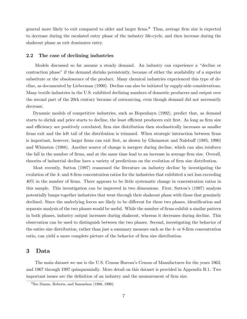
general more likely to exit compared to older and larger firms.9 Thus, average firm size is expected
to decrease during the escalated entry phase of the industry life-cycle, and then increase during the
shakeout phase as exit dominates entry.
2.2 The case of declining industries
Models discussed so far assume a steady demand. An industry can experience a “decline or
contraction phase” if the demand shrinks persistently, because of either the availability of a superior
substitute or the obsolescence of the product. Many chemical industries experienced this type of de-
cline, as documented by Lieberman (1990). Decline can also be initiated by supply-side considerations.
Many textile industries in the U.S. exhibited declining numbers of domestic producers and output over
the second part of the 20th century because of outsourcing, even though demand did not necessarily
decrease.
Dynamic models of competitive industries, such as Hopenhayn (1992), predict that, as demand
starts to shrink and price starts to decline, the least efficient producers exit first. As long as firm size
and efficiency are positively correlated, firm size distribution then stochastically increases as smaller
firms exit and the left tail of the distribution is trimmed. When strategic interaction between firms
is important, however, larger firms can exit first, as shown by Ghemawat and Nalebuff (1985, 1990)
and Whinston (1988). Another source of change is mergers during decline, which can also reinforce
the fall in the number of firms, and at the same time lead to an increase in average firm size. Overall,
theories of industrial decline have a variety of predictions on the evolution of firm size distribution.
Most recently, Sutton (1997) reassessed the literature on industry decline by investigating the
evolution of the 4- and 8-firm concentration ratios for the industries that exhibited a net loss exceeding
40% in the number of firms. There appears to be little systematic change in concentration ratios in
this sample. This investigation can be improved in two dimensions. First, Sutton’s (1997) analysis
potentially lumps together industries that went through their shakeout phase with those that genuinely
declined. Since the underlying forces are likely to be different for these two phases, identification and
separate analysis of the two phases would be useful. While the number of firms exhibit a similar pattern
in both phases, industry output increases during shakeout, whereas it decreases during decline. This
observation can be used to distinguish between the two phases. Second, investigating the behavior of
the entire size distribution, rather than just a summary measure such as the 4- or 8-firm concentration
ratio, can yield a more complete picture of the behavior of firm size distribution.
3 Data
The main dataset we use is the U.S. Census Bureau’s Census of Manufactures for the years 1963,
and 1967 through 1997 quinquennially. More detail on this dataset is provided in Appendix B.1. Two
important issues are the definition of an industry and the measurement of firm size.
9See Dunne, Roberts, and Samuelson (1988, 1990).
7

3.1 Industry definition
Models of industry evolution usually focus on a homogenous product or a group of products
that are very closely related. The industry classification system (SIC) of 1987, which we adhere to
consistently throughout the sample period, consists of 5 levels of aggregation for individual products.
A “product” is usually defined uniquely by a 7-digit code. Similar products are grouped into “product
classes”, identified by their common 5-digit code. There were 1,446 such classes in the 1987 SIC
system. These product classes are further grouped into 459 “industries” according to the first 4 digits
of the product class code.10 This 4-digit level is the level of aggregation we focus on.
Some 4-digit industries contain a single product, and some contain several products that are closely
related. Our focus on a 4-digit industry reflects a desire to keep the industry definition narrow enough
to maintain connection to the theory, but flexible enough to include closely related products. The
4-digit level industry classification is generally coarser than the product level analysis of Gort and
Klepper (1982). However, it can be argued that even a narrowly defined product category can consist
of several products. For instance, the fluorescent lamp, one of the products used by Gort and Klepper
(1982), is essentially a product category and contains many different types of lamps in various sizes,
shapes, and capacities. Nevertheless, these products are very close substitutes and it makes sense to
treat them as a single category.
Our final sample consists of 322 industries out of a total of 459 4-digit industries defined by the
1987 SIC system. Several reasons led us to drop a number of industries to improve data quality.
Some industries were found to have problems in their product codes by other researchers. Some are
collections of firms that manufacture eclectic products that are not classified elsewhere. To maintain
uniformity of products within an industry as much as possible, we excluded these industries. Finally,
some industries had missing observations and a few of them exhibited substantial discontinuities in
the time series for number of firms and output due to revisions in SIC codes. Appendix B.1 provides
more detail on the selection process that led to our sample.
3.2 Measures of firm size
Theories focus on a firm as the unit of analysis rather than a plant. To maintain consistency with
the models, we aggregated plant-level data to firm level using firm identifiers assigned to each plant.
We follow two main procedures for classifying plants into industries. The first one is the “primary-
SIC-code-based classification”, which assigns a plant into a 4-digit industry if the plant’s highest value
of shipments among all products it produces falls into that industry. This approach is also the main
method followed by the Census Bureau in classifying plants into 4-digit industries, assuming that each
10On average, there were 3.15 5-digit product classes within a 4-digit industry in the 1987 SIC system. This average
was highest (5.00) for the 4-digit industries classified under the 2-digit group Printing and Publishing industries, and
lowest (1.09) for the 4-digit industries classified under the 2-digit group Leather and Leather Products. A full list of
7-digit and 5-digit product groups classified under each 4-digit industry is available from the U.S. Census Bureau’s 1987
supplement publications to the 1987 Census of Manufacturers.
8

plant is a single-product manufacturer rather than a multi-product one. This assumption in general
understates the number of firms and the entry rate in an industry, and overstates the exit rate. These
shortcomings are important when industry evolution is the focus. Nevertheless, this first approach
has been used by researchers. To remedy the shortcomings of the first approach, our second approach
takes into account all the 4-digit industries a plant produces in, and thus considers each plant as a
multi-product producer. The classification of a plant into each 4-digit industry it produces in is done
using product level data that provides the value of shipments of each plant by 7-digit product category,
which can be aggregated to the 4-digit level. We report our results for both classification schemes.
The ideal theoretical measure of firm size is output rather than employment or sales. While both
employment and sales have traditionally been used as measures of firm size, relatively little is known
about the relationship among different measures of firm size. If firm productivity increases along the
life-cycle, and especially if the increase is non-uniform across firms of different sizes, firm employment
may not be the best measure of firm size heterogeneity. Sales, on the other hand, suffer from the
effects of price changes over time. While output usually has a predictable path of positive growth
trend throughout the industry life-cycle, as shown in Figure 1, sales may increase or decrease over
time, depending on the elasticity of demand. Analysis of sales data is further complicated by inflation.
To assess the relative merits of different size measures, we consider both employment and output
as measures of size. Firm employment is the total employment of a firm’s plants classified in a given
4-digit industry. It is straightforward to calculate a firm’s employment when the employment of
each of its plants is assumed to be fully devoted to the production activity in its primary SIC code.
When plants are considered as multi-product manufacturers, a choice has to be made to allocate the
plant’s employment to the production of each product, because the Census Bureau does not collect
information on the number of employees engaged in the production of each product. We chose to
allocate employment in proportion to each product’s share in the plant’s total value of shipments.11
Firm output is obtained from the total value of shipments of a firm’s plants using 4-digit industry
price deflators for the shipments available from the NBER/CES Manufacturing Productivity Database.
This database is described in Appendix B.2. The price deflator for an industry allows us to construct a
time series for firm value of shipments in 1987 dollars. Thus, we can identify the output of a firm up to
a constant under the assumption that the industry price is common to all firms in a given census year.
The details of the construction of firm output and industry price deflators are discussed in Appendix
B.1.2. The NBER/CES dataset was also used to obtain industry real price series, as described in
Appendix B.2.1.
11This allocation can result, for instance, from a Cobb-Douglas production function specification for a plant, such as
Yi = ALαii K
1−αii , where i = 1, ...,m indexes the products, Li is the labor devoted to product i, Ki is the capital devoted
to product i, αi ∈ (0, 1) is labor’s share in the value of product i, and A is a fixed factor. Then, one can write, under acommon wage rate for all labor, Li =
αiPiYiPmj=1 αjPjYj
, where Pi is the price of product i.
9

4 Empirical methodology
Our empirical analysis comprises three main steps. First, industries are classified according to
the life-cycle phase(s) they had gone through during the sample period. Second, changes in the firm
size distribution during these life-cycle phases are analyzed. Finally, differences in the behavior of firm
size distribution in different life-cycle stages are documented.
4.1 Identification of life-cycle phases
Gort and Klepper (1982) originally identified 5 life-cycle “stages”, as shown in the upper panel
of Figure 1. Instead, we focus primarily on three “phases”, as shown in the lower panel of Figure
1, where a phase spans one or more stages. The main reasons for our focus on a small number of
phases, rather than all five original stages, are as follows.12 First, our data consists of quinquennial
observations, as opposed to annual observations in Gort and Klepper (1982), which do not allow us to
fine-tune the identification of phases. Second, Stage I, as identified by Gort and Klepper (1982), had
primarily disappeared in most products roughly by 1963 in which our sample period starts.13 Third,
it is inherently difficult to identify the period of temporary stability in the number of firms before
the shakeout (Stage III) from the eventual stability (Stage V). Accordingly, our Phase I is the initial
growth phase during which the number of firms in the industry increases, corresponding to Stages
I and II, and early parts of Stage III; Phase II is the shakeout during which the number of firms
decreases, corresponding to all of Stage IV, and later parts of Stage III and early parts of Stage V;
and finally, Phase III is the phase of stability or maturity corresponding to Stage V, during which
the number of firms does not change substantially. It is important to note that the life-cycle stages
or phases sketched in Figure 1, while typical, need not occur in every single industry. For instance,
there are some industries that have not gone through a shakeout phase.14 Phase III also includes the
case where an industry does not experience a shakeout, but only a stability in the number of firms
following Phase II. Our approach does not assume a priori that all three phases must be observed.
The time series available to us is not long enough to observe the entire life-cycle of an industry.
Instead, we observe a 35-year-long episode from the life-cycle. We therefore need to identify the trends
in the number of firms and output during these 35 years to classify the observed episode into life-cycle
phase(s). It is possible to identify the underlying trend in the number of firms using a time-series filter
such as the Hodrick and Prescott (HP) filter. Denote the number of firms in the industry at time t
by Nt, for t = 1, 2, ..., T. Nt is assumed to follow the process
Nt = N∗t + εt,
12In fact, Gort and Klepper (1982) admit that the number of stages or phases they identify is not definitive, and can
depend on the nature and the frequency of the data, as well as a researcher’s goal.13See Agarwal and Gort (1998) for evidence on the gradual disappearence of this phase.14Gort and Klepper (1982) found that there was little or no shakeout in the baseboard radiant heater, electrocardio-
graph and fluorescent lamp industries.
10

where N∗t is an underlying “smooth” function of t that describes the life-cycle behavior of the number
of firms, and εt is a zero-mean error component that captures deviations from this trend.15 Following
Hodrick and Prescott (1997), the trend is the solution to the optimization problem
min{N∗t }
Tt=1
(TXt=1
ε2t + λTXt=2
£(N∗t+1 −N∗t )− (N∗t −N∗t−1)
¤2)
where λ > 0 is a parameter that penalizes variability in N∗t .16
We use the procedure described above to also uncover the trend, Q∗t , in industry output, Qt. After
the estimates cN∗t and cQ∗t are obtained, the life-cycle phases can be identified, based on the jointbehavior of cN∗t and cQ∗t . If cQ∗t is increasing and cN∗t is increasing (decreasing), then the industry is inPhase I (Phase II). If cQ∗t is increasing and cN∗t is relatively stable or exhibits no clear trend, then theindustry is in Phase III. If both cN∗t and cQ∗t are decreasing, then the industry is in a decline phase.
Figure 4 contains sample paths for the number of firms that are, while not actual, representative
of what we observed in most of our sample of industries.17 In some cases, the number of firms did not
seem to fluctuate much and the trend was easily identified. In others, the number of firms exhibited
fluctuations, potentially attributable to business-cycle effects. In such cases, we relied more heavily on
the HP-filter to determine the underlying trend. In cases where classification was not straightforward,
we used several different values for the smoothing parameter λ to make sure that the classification is
made as accurately as possible. While the classification method is not error-free, in most cases the
trends were obvious and strong. Overall, we found that for most industries the trend in number of
firms for the entire period of 35 years for an industry can be classified as either Phase I, Phase II,
Phase III, or Phase I combined with Phase II. More detail on the classification is provided in the
section on empirical results.
Samples of time-paths for output are shown in Figure 5. These examples were produced using
the value of shipments and price deflator data from the NBER/CES productivity database, which
is publicly available. Output data computed from the Census of Manufactures, which we use for
our empirical analysis, exhibits similar behavior, but is only available in census years. Since the
NBER/CES data have a higher frequency (annual) and a longer time span, we chose to use it only to
generate figures, but to avoid any discrepancies between the two datasets we did not use it to construct
the output figures actually used in our empirical analysis.18 As in the case of the number of firms, the
15We treat the number of firms Nt as a continuous variable in this specification.16A practical issue is the choice of the smoothing parameter λ. Arguments in Ravn and Uhlig (2002) suggest a value
of λ in the range [0.01, 0.0182] for quinquennial data. We found that this suggestion did not yield satisfactory results
in many cases: the smoothed series were very close to the original series, simply because as λ gets closer to zero the
smoothed series approach the original series. Instead, for each industry we experimented with several values in the range
[1, 5] and found that usually λ = 2.5 to 3 worked well in most cases.17Restrictions imposed by the Census Bureau on the disclosure of research output preclude us from presenting a wide
range of detailed industry level data.18We compared the output and employment figures at the 4-digit industry level for the Census of Manufacturers and
the NBER/CES database. We found that these measures did not match perfectly across the two datasets. The reason
11

output generally exhibited three distinct trends throughout the sample period of 35 years: increasing,
decreasing, and relatively stable. In a few cases, there was also a non-monotonic (inverted U-shaped)
pattern, as we discuss in the empirical results.
4.2 Analysis of the size distribution
Following the classification of industries into phases, a series of statistical analyses are performed
on the firm size distribution.
4.2.1 Moments of firm size
Let Xt be a random variable that represents firm size in an industry at time t, and let Ft(x)
be its distribution function. Throughout the rest of the paper, we use the following theoretical def-
initions: the mean µt = E[Xt], the median mt = inf{x : Ft(x) ≥ 0.5}, the standard deviation
σt =¡E[(Xt − µt)2]
¢1/2, the coefficient of variation cvt =
σtµt, the skewness γt =
E[(Xt − µt)3]σ3t
, and
the kurtosis κt =E[(Xt − µt)4]
σ4t. We use the following estimates of these moments:
bµt =1
Nt
NtXj=1
xjt, bmt = {x(Nt/2+1) if Nt is odd,x(Nt/2) + x(Nt/2+1)
2otherwise}, (1)
bσt =
⎛⎝ 1
Nt − 1
NtXj=1
(xjt − bµt)2⎞⎠1/2
, bcvt = bσtbµt ,bγt =
1
Nt
NtXj=1
µxjt − bµtbσt
¶3, bκt = 1
Nt
NtXj=1
µxjt − bµtbσt
¶4.
Most of these empirical moments follow the usual conventions. The coefficient of variation is important
for our purposes, because in many cases, mean and the standard deviation both change over time and
a meaningful measure of dispersion in firm size is the variation in firm size with respect to the average
firm in the industry. Skewness captures whether the firm size distribution is symmetric around its
mean. A positively (negatively) skewed distribution corresponds to one that assigns more of the total
probability to the left (right) of the mean, i.e. more toward smaller (larger) firms. Kurtosis measures
the degress of peakedness or the thickness of the tails of the distribution. A higher value of kurtosis
means a less peaked, flatter distribution with more probability assigned to tails. Note that for kurtosis
κt, we use “kurtosis proper”, rather than “kurtosis excess”, which is the value in excess of the kurtosis
of the normal distribution. Since most of our analysis involves the growth rate of kurtosis, this choice
is inconsequential.
is that the NBER/CES database does not use the census data at the firm level directly to calculate these measures. See
Appendix B and Bartelsman and Gray (1996) for details.
12

4.2.2 Stochastic trends
In addition to the changes in individual moments of firm size, an important question is whether
the size distribution as a whole is changing significantly over time, in a first-order stochastic-dominance
sense. Specifically, for two points in time, t = 1 and t = T, we want to test the hypotheses
Ho : FT (x) = F1(x) for all x. (2)
Ha : FT (x) 6= F1(x) for some x.
We use relatively flexible methods capable of capturing movements in the size distribution regardless
of the exact type of change the distribution is undergoing. One of the distance-based measures that
can be used to test this hypothesis is the Kolmogorov-Smirnov (KS) test.19 Define the empirical
counterpart of Ft at any point x in the support of the firm size distribution by
bFt(x) = 1
Nt
NtXj=1
I(xjt ≤ x),
where I(·) is the indicator function. Let St be the set of observed firm sizes at time t = 1, T. The KS
test-statistic is given by
D = maxx∈(S1∪ST )
¯̄̄ bFT (x)− bF1(x)¯̄̄ . (3)
An attractive feature of the statistic D is that its distribution does not depend on the exact
distribution of firm size.20 This property is particularly useful for our purposes because the shape
of the size distribution varies from one industry to another, as well as over time. An important
assumption behind the KS test is the independence of the two samples, which can be violated in our
setting, since the set of firms active at time t = T is likely to contain firms that were also around at
time t = 1. The fact that we measure the size distributions at two points in time that are sufficiently
far apart (35 years) alleviates the concerns about dependence to some extent, but certainly does not
eliminate it.21
19A chi-square test is also feasible. However, the KS test has certain advantages over the chi-square test. First, the
KS test does not require data that come in groups or bins, while the performance of the chi-square test is affected by
the number of bins and their widths. Second, the KS test can be applied for small sample sizes, whereas the chi-square
test is more appropriate for larger samples. For more on the KS test, see, e.g., Gibbons (1971) and Siegel and Castellan
(1988).20The critical values of the KS test statistic are available in standard texts on nonparametric statistical analysis as
well as in common statistical software. See, for instance, Tables LI to LIII in Siegel and Castellan (1988), pp. 348 to 352.
We used STATA to calculate the KS statistics values and their significance. STATA allows for a better approximation
of critical values of the KS statistic for small samples. We used this improved approximation when the number of firms
at time t = 1 or t = T was less than 100.21Methods have been recently developed to obtain consistent KS test statistics under general dependence of the two
samples (see, e.g., Linton, Maasoumi, and Whang (2003)). However, they are computationally demanding, so we did not
implement them for this analysis.
13

The second issue of interest is the direction of change in the size distribution, in a first-order
stochastic sense. Higher orders of stochastic dominance, such as second-order or third-order, can also
be investigated using recent techniques. However, theories do not have obvious predictions on these
higher order shifts, so we focus only on first order dominance. A one-sided version of the KS test can
be used to test for first-order stochastic dominance. Define
D− = maxx∈(S1∪ST )
( bFT (x)− bF1(x)) (4)
for testing Ho in (2) against the alternative
Ha : FT (x) ≥ F1(x), for all x, and FT (x) > F1(x) for some x.
Similarly define
D+ = maxx∈(S1∪ST )
( bF1(x)− bFT (x)) (5)
to test against the alternative
Ha : FT (x) ≤ F1(x), for all x, and FT (x) < F1(x), for some x.
A sufficiently large positive value of D− favors a stochastically decreasing firm size going from t = 1 to
t = T . On the other hand, a sufficiently large positive value for D+ favors a stochastically increasing
firm size. However, note that D− and D+ can be simultaneously large. This can happen, for instance,
if the two distribution functions cross at a single point and the maximum distances between them on
both sides of this point are large. To identify cases in which only one of D− and D+ is significantly
large, we use the following simple approach: FT stochastically dominates F1 if D+ is statistically
significant at some level α% or lower, and at the same time, D− is not significant at α% or lower
levels. A similar definition applies to the case where F1 stochastically dominates FT .
4.3 Life-cycle effects
After identifying the life-cycle phases and obtaining the statistics pertaining to the size distribu-
tion, we summarize compactly the behavior of the size distribution by life-cycle phase. Let ∆y denote
the percent growth rate for the empirical moment y = bµ, bm, bσ, bcv, bγ, bκ between the two end points ofour sample, 1963, corresponding to t = 1, and 1997, corresponding to t = T. Denote the expected
value of ∆y by µ∆y, which can be viewed as the mean of the underlying random process that generates
the growth rates ∆y for industries. For each life-cycle phase, we describe the average behavior of ∆y,
and test the hypotheses
Ho : µ∆y = 0,
Ha : µ∆y 6= 0.
14

We also compare the average value of ∆y across phases, and identify any asymmetries in the behavior
of the moments across phases. Similarly, we summarize the patterns of stochastic movements in firm
size by life-cycle phase based on the KS tests.
Another issue of interest is whether the extent of the change in each moment of the size distribution
over time is related systematically to the extent of the life-cycle phase. The models discussed earlier,
in particular Jovanovic and MacDonald (1994a), suggest that the magnitude of change in the moments
should depend on the direction and magnitude of the change in the number of firms during a life-cycle
phase, which in turn depends on industry-specific fundamentals such as the rate of innovation and the
difference between the scales of high-tech and low-tech firms. Since most of these fundamentals are
not observable in our data, it is not possible to directly relate the changes in the moments to them.
Nevertheless, the magnitude of the change in the number of firms and industry output should reflect
the strength of these fundamentals. For instance, we expect to observe a more pronounced change in
the moments of firm size distribution in an industry that experiences a mass exit of a large fraction of
firms compared to an industry that loses only a small fraction of firms. In Jovanovic and MacDonald
(1994a), for example, a higher rate of adoption of the better technology and a larger gap between the
sizes of high-tech and low-tech firms lead to a more severe and faster decline in number of firms, a
larger growth rate in output, as well as a higher rate of increase in average firm size.
We measure the extent of the life-cycle phase using the percent change in the number of firms,
∆N, and in output, ∆Q, during a life-cycle phase. We relate each ∆y to ∆N and ∆Q for a given
life-cycle phase using a simple projection of the form
∆yi = α+ βN∆Ni + βQ∆Qi + βNQ(∆Ni∆Qi) + εi, (6)
where i indexes the industries and εi is a projection error that represents the effect of unobservables.
We include ∆N and ∆Q simultaneously in the projection, as well as an interaction term, because
two industries exhibiting similar behavior in the number of firms are likely to differ with respect to
∆y if the rates of change in output differ. The coefficients of interest are βN , βQ, and βNQ, which
describe the association of the extent of the change in a moment to the extent of the life-cycle effects
as measured by ∆N and ∆Q.
5 Examples
To illustrate our general analysis, we first consider two detailed examples. For these examples,
we classify plants based on their primary 4-digit industry. The results are very similar if we instead
classify plants into multiple industries based on all SIC codes they produce in.
15

5.1 Example 1: Electronic computers
The evolution of key variables in the Electronic Computers industry (SIC 3571) is shown in Figure
7.22 The number of firms exhibited a non-monotonic pattern, and parts of Phases I and II are both
clearly visible, even though they are not observed in their entirety. The number of firms peaked around
1982, and a shakeout followed, resulting in an exit of roughly half of the firms at the peak. In the
meantime, output increased exponentially, and price fell sharply.23 The distribution of the logarithm
of firm employment is highly skewed for all three census years considered. Between 1963 and 1982
(Phase I), firm employment tended to decrease stochastically, while between 1982 and 1997 (Phase II),
it appears to have exhibited a slight stochastic increase. In contrast to the employment distribution,
the output distribution tended to stochastically increase during both phases of the life-cycle. The
number of plants per firm also declined steadily throughout the two phases, rebounding slightly after
1992.
Figure 8 considers the evolution of firm employment distribution in more detail.24 While the
employment distribution mostly shifted left during the 1963-1982 period, it tended to shift right
between 1982 and 1997, after the number of firms reached its peak. Overall, the shift was not generally
monotonic, however, as indicated by the rightward shift between 1982 and 1987, followed by a leftward
shift thereafter.
The evolution of the moments of firm employment (in levels) shown in Figure 9 reveals an interest-
ing asymmetry between the two phases of the life-cycle. Before 1982, the mean, the median, and the
standard deviation of firm employment declined from their 1963 levels, while the coefficient of varia-
tion, the skewness, and the kurtosis increased. After 1982, all these trends appear to have reversed.
In other words, during Phase I of the life cycle firm employment became increasingly skewed towards
smaller firms, more dispersed relative to its mean, and had an increasingly heavier tail, whereas during
Phase II of the life-cycle it became more symmetric, less dispersed relative to its mean, and eventually
had a thinner tail compared to the peak year 1982.
The distribution of the logarithm of firm output exhibits an almost monotonic rightward shift
during both phases, as shown in Figure 10. The evolution of the moments of firm output (in levels)
is shown in Figure 11. Unlike in the case of firm employment, the median and the standard deviation
of firm output increased steadily beginning in 1963, and while the mean initially declined slightly, it
overall exhibited a strong upward trend. Average firm output in 1997 was about 13 times its value
22According to the 1987 SIC system, this industry is composed of two related 5-digit products: “Computers (excluding
word processors, peripherals and parts)” and “Parts for computers”. Thus, the industry consists of a relatively narrow
range of related products.23The output and price data are from the NBER/CES Manufacturing Productivity database. As mentioned earlier,
we use the NBER/CES output data to generate only the graph pertaining to the evolution of the output, because
the NBER/CES data has annual observations. For the examples, the pattern of output time-series is similar in the
NBER/CES data and the Census of Manufacturers.24The bandwidths used in kernel density estimates are in most cases higher than the optimal plug-in bandwidth. This
extra smooting is required to avoid the disclosure of firms’ sizes, especially towards the tails of the density estimates.
16
in 1963, and the standard deviation of output actually increased by about 18 times. The behavior of
the higher moments, though, is remarkably similar to the case of firm employment. The coefficient of
variation, the skewness, and the kurtosis all increased during Phase I, peaking in 1982 and thereafter
declined till the end of the sample period.
The evolutions of the computer industry and the automobile tire industry discussed in Appendix
A look alike in many ways, especially in terms of the time-paths of the number of firms, output, and
price. A comparison of the evolutions of the estimated moments of firm output in Figure 2 and in
Figure 11 also reveals substantial similarity. In both cases, average firm size tended to rise over time.
While the standard deviation behaved somewhat differently across the two industries, the coefficient
of variation, skewness, and kurtosis all moved in the positive direction initially and then reversed their
trends. The resemblance of the patterns exhibited by these two entirely unrelated industries going
through similar life-cycle phases encourages the examination of other industries for evidence of further
empirical regularity.
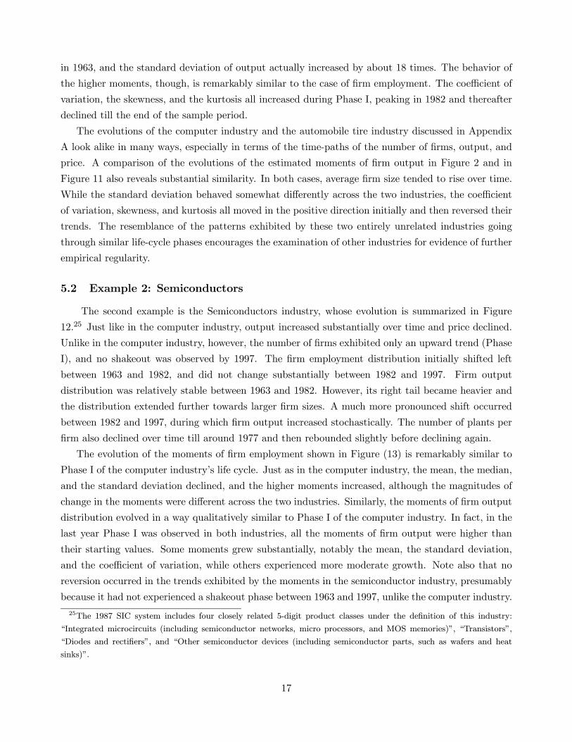
5.2 Example 2: Semiconductors
The second example is the Semiconductors industry, whose evolution is summarized in Figure
12.25 Just like in the computer industry, output increased substantially over time and price declined.
Unlike in the computer industry, however, the number of firms exhibited only an upward trend (Phase
I), and no shakeout was observed by 1997. The firm employment distribution initially shifted left
between 1963 and 1982, and did not change substantially between 1982 and 1997. Firm output
distribution was relatively stable between 1963 and 1982. However, its right tail became heavier and
the distribution extended further towards larger firm sizes. A much more pronounced shift occurred
between 1982 and 1997, during which firm output increased stochastically. The number of plants per
firm also declined over time till around 1977 and then rebounded slightly before declining again.
The evolution of the moments of firm employment shown in Figure (13) is remarkably similar to
Phase I of the computer industry’s life cycle. Just as in the computer industry, the mean, the median,
and the standard deviation declined, and the higher moments increased, although the magnitudes of
change in the moments were different across the two industries. Similarly, the moments of firm output
distribution evolved in a way qualitatively similar to Phase I of the computer industry. In fact, in the
last year Phase I was observed in both industries, all the moments of firm output were higher than
their starting values. Some moments grew substantially, notably the mean, the standard deviation,
and the coefficient of variation, while others experienced more moderate growth. Note also that no
reversion occurred in the trends exhibited by the moments in the semiconductor industry, presumably
because it had not experienced a shakeout phase between 1963 and 1997, unlike the computer industry.
25The 1987 SIC system includes four closely related 5-digit product classes under the definition of this industry:
“Integrated microcircuits (including semiconductor networks, micro processors, and MOS memories)”, “Transistors”,
“Diodes and rectifiers”, and “Other semiconductor devices (including semiconductor parts, such as wafers and heat
sinks)”.
17

The examples therefore raise the possibility of systematic differences in the behavior of the moments
during different phases of the life-cycle.
6 Results
In this section, we seek to uncover any regularities for the entire sample of industries available to
us.
6.1 Evolution of the moments
We first consider the primary-SIC-code-based classification. Using the methodology described in
Section 4.1, we were able to classify 322 4-digit industries into four basic groups based on the pattern
the number of firms exhibited: 140 industries with a general growth trend in the number of firms,
119 industries with a general decline trend, 53 industries with relatively stable pattern or no obvious
trend, and 10 industries with a clear non-monotonic path, i.e. first increasing and then decreasing
number of firms. Note that all of these patterns are consistent with what we expect to observe if
life-cycle effects are present in the data. For instance, a V-shaped time path for the number of firms
would be at odds with the general life-cycle pattern for the number of firms, and we indeed did not
observe such a pattern in any of the industries.
Between 1963 and 1997, the number of firms grew by 170.3% on average in industries in which the
number of firms exhibited a growth trend, and it declined by 47.8% in industries where the number of
firms tended to decline. In industries with relative stability and little trend group, there was a slight
increase (∼12%) in the number of firms on average, whereas in the non-monotonic case, the averageincrease was about 60%. At the same time, 270 industries exhibited a growth trend in output, 32 had
a persistent decline in output, and in 20 industries output had a non-monotonic, inverted U-shaped
path of an increase followed by a decline. The pattern of U-shaped output does not readily fit the
general monotonic behavior of output over the life-cycle, but such cases only account for only 6% of
all industries.
Consider now the classification of industries into life-cycle phases. In Table 3, industries are grouped
by the pattern the number of firms exhibits as well as the pattern of output. We were able to identify
4 major groups of industries. 127 industries exhibited both growing number of firms and output, 91
industries experienced a decline in number of firms but a growth in output, 22 industries declined
in both measures, and 44 industries exhibited no obvious trend in number of firms, but experienced
growth in output.26
26Some industries did not fall into any one of these four groups. These industries exhibited the following patterns: non-
monotonic (inverted-U) number of firms and growing output (8 industries); growing number of firms and non-monotonic
(inverted-U) output (10 industries); declining number of firms and non-monotonic (inverted-U) output (5 industries);
stable number of firms and declining output (5 industries), non-monotonic (inverted-U) number of firms and declining
output (4 industries), non-monotonic (inverted-U) number of firms and non-monotonic (inverted-U) output (1 industry),
18

In industries that went through Phase I, the output increased on average by about 20 times,
whereas in it increased by about 10 times on average in Phase II and about 2.5 times during Phase
III. In the decline phase, the output at the end of the sample period was about half the initial output
on average. We also calculated real price series for each industry using the procedure described in
Appendix B.2.1. In Phase I, real price decreased by about 25% on average, and by about 30% in
Phase II. In Phase III, the average rate of fall in price was about 11%, and about 20% during the
decline phase. The observed trends in output and price are broadly consistent with their theoretical
path throughout the life-cycle and also with the trends discovered in Gort and Klepper (1982).
Note the markedly different patterns in moments of firm size in Phase I versus Phase II. Table
3a indicates that, on average, employees per firm declined in Phase I, but increased in Phase II. The
dispersion of firm employment as measured by the coefficient of variation also increased in Phase I
by about 33%, but did not change significantly on average in Phase II. Skewness and kurtosis moved
in opposite directions during these two phases. In Phase III, the mean, the median and the standard
deviation did not change significantly, although the higher moments exhibited some positive growth,
similar to Phase I. In the decline phase, average firm employment did not change substantially, and
the only significant trends are observed in skewness and kurtosis, both of which moved in the positive
direction on average, indicating increasingly symmetric and thinner-tailed employment distribution as
the decline progresses.
For the case of output, the statistics in Table 3b indicate that average and median firm output
grew on average in all phases, but the rates of growth were different. The highest growth rate in
average output is observed in Phase II, followed by Phase I. While average output grew by about the
same amount in Phase III and in the decline phase, the median employment grew about 6 times more
in the case of declining industries. The ranking of the growth in the standard deviation across phases
points to a large increase for Phase I , followed by Phase II, Phase III, and the decline phase. However,
the increase in Phase I has the lowest statistical significance. The coefficient of variation increased
substantially during Phase I and Phase III, but it did not change by much in industries experiencing
Phase III or decline. Also notable is the similarity of the changes in skewness and kurtosis in Phases
I and III, and in Phase II and the decline phase. In Phases I and III, both moments tend to increase,
although much more in absolute value in the case of Phase I. In Phase II and the decline phase, they
both decrease, but at a higher rate on average in the decline phase.
Table 3c compares the trends in the moments for Phases I and II. The difference in average growth
rates of moments (Phase I minus Phase II) are mostly significant, except for the mean and the standard
deviation of output, even though the magnitudes of the differences in these two moments are quite
large.
growing number of firms and declining output (2 industries), stable number of firms and non-monotonic (inverted-U)
output (3 industries). Most of the patterns regarding moments of firm employment and output in these industries were
not statistically significant, due probably to a small number of observations in each case. As a result, we do not discuss
these groups of industries.
19

Tables 4 repeats the analysis of the evolution of moments for the alternative classification of plants
into industries based not only on their primary products, but also the other products they produce.
As discussed earlier, this approach addresses concerns about any understatement in the number of
firms and entry rates, and overstatement in exit rate when the primary-SIC-code-based classification
is used. We re-classified industries into the same groups as in Table 3. The re-classification resulted in
some change in the number of industries falling into different life-cycle phases, especially into Phases II
and III. Such differences are expected because in certain industries the number of firms may be more
responsive more to the classification scheme. A comparison of Tables 3 and 4 reveal a qualitatively
similar pattern across the two classification schemes. While the absolute values and the significance of
the growth rates differ across the comparable panels, the directions of shifts observed in the moments
and the relative magnitudes of the growth rates in moments for different phases are in general robust
to the classification scheme. The most notable discrepancy occurs in the case of Phase III. In the new
classification, the mean and the standard deviation of firm employment appears to have grown on
average, while in the primary-SIC-code-based classification these moments did not exhibit substantial
change.
6.2 The implied evolution of firm size
What is the implied evolution of firm size distribution given the changes in the moments described
in the previous section? To be able to answer this question, we need to describe the typical initial
distribution of firm size in an industry. However, the precise shape of firm size distribution in a
young industry cannot be obtained from the data available to us. Nevertheless, we can describe the
general shape of firm size distribution for a manufacturing industry and use this shape as a benchmark.
Consider the following normalization of firm size Xt in an industry at time t :
Xnt =
Xt − LtHt − Lt
=Xt − LtRt
,
where Lt and Ht are the lower and upper bounds of the compact support of Xt, and Rt = Ht − Lt.27
This normalization maps the support of Xt onto the interval [0, 1] and facilitates the comparison of
firm size distribution both over time and across industries. It is easy to show that the following
relationships between the moments of Xt and Xnt hold:
µnt =1
Rt(µt − Lt),σnt =
1
Rtσt, cv
nt =
σtµt − Lt
, γnt = γt,κnt = κt. (7)
An empirical analog to normalized firm size can be constructed from observed firm sizes xt as follows
xnt =xt − xmint
xmaxt − xmint
,
27This definition rules out unbounded supports, but in general technological and organizational limits on firm size
imply a compact support for the theoretical distribution of firm size.
20

where xmaxt and xmint are the observed maximum and minimum firm sizes, respectively. While xnt is
neither an unbiased nor a consistent estimate of Xnt , it is a practical estimator that helps us compare
the two empirical size distributions across industries and over time. As before, we use the definitions
in (1) to obtain the empirical moments based on xnt .
Table 5 provides the average moments of the normalized firm size across all 4-digit industries for
three different census years. Note that the normalized employment has, on average, higher mean and
higher standard deviation than the normalized output, but lower coefficient of variation. Both of the
normalized sizes are highly positively skewed on average, but the normalized employment is less skewed
than the normalized output. The normalized employment has also lower kurtosis compared to the
normalized output. All of these average moments are very precisely estimated and the hypothesis that
any given moment differs across the two normalized sizes for all three census years is easily rejected
using paired t-tests. There has been a slight decline in both of the average normalized sizes over time,
but the dispersion relative to the mean, skewness, and kurtosis have all increased.
The pattern in Table 5 indicates that firm employment and output in a typical manufacturing
industry are highly positively skewed at any point in time. Therefore, it is not unreasonable to assume
that typical initial firm size distribution in a young industry is also highly positively skewed. The
evolution of the moments observed so far, then, draw the following picture for the behavior of firm
employment and output along the life-cycle: As an industry experiences Phase I of its life-cycle,
firm employment declines on average, and it becomes more dispersed relative to its mean, indicating
an increase in firm size heterogeneity. In the meantime, average firm output increases and, like
employment, becomes much more dispersed relative to its mean. Skewness of both employment and
output become even more positive and asymmetry in firm size distribution increases. Kurtosis of
both size measures also increase, indicating a heavier right tail. As Phase II of the life-cycle sets on,
however, the trend in average firm employment reverses: firms become larger on average. Firm output,
on the other hand, continues to increase at a much higher rate compared to Phase I. Dispersion in
firm output and employment subsides, both distributions become more symmetric, and the right tail
gets thinner.
When the industry is in Phase III, average firm output continues to grow, but at a lower rate
on average than in Phases I and II. Other moments of firm employment and output do not usually
stabilize entirely in this phase. The coefficient of variation, skewness, and kurtosis all exhibit positive
growth rates on average, both for employment and output. Finally, in the decline phase, average
employment tends to decline slightly and other moments do not exhibit significant change, except
for skewness and kurtosis, which tend to move in the negative direction on average. Firm output in
declining industries, on the other hand, increases significantly on average, and its dispersion relative
to its mean increases only slightly. Firm output distribution also becomes more symmetric and less
peaked during decline.
21

6.3 Stochastic trends
Are the documented changes in the moments of firm employment and output accompanied by
first-order stochastic shifts in firm employment and output distribution? Such shifts need not occur
even when some moments of firm size change significantly. Table 6 summarizes the stochastic trends in
firm size distribution by phase for the primary SIC code classification. The column labelled “Change”
provides the percentage of industries within a group that exhibited a statistically significant change
in firm size distribution based on the test statistic D in (3). The columns labelled “Increase” and
“Decrease” give the percentage of industries which experienced a statistically significant stochastic
increase and decrease, respectively, in firm size, based on the convention we adopted using the test
statistics D− and D+ defined in (4) and (5).
Table 6a summarizes the trends in employment distribution. During Phase I, employment stochas-
tically declined in about 63% of the cases, and increased in only 20%. Phase II, on the other hand,
is characterized by a more even allocation of industries: in about 50% of the industries, firm employ-
ment stochastically increased, and in about 40% it declined. Even in the case of stable industries
(Phase III), most industries experienced a stochastic decrease in employment, similar to Phase I. Firm
employment also tended to decline stochastically in most of the declining industries.
Trends in firm output in Table 6b also point to systematic differences across life-cycle phases. In
Phase I, output increased stochastically in about 45% of the industries, and decreased in 37%. In
Phase II, however, there was a clear tendency for output to stochastically increase. In about 87%
of the industries, firm output distribution was stochastically higher in 1997 then in 1963. Again,
most of the industries exhibited a stochastically increasing output in Phase III, but there was also a
considerable number of cases where output stochastically declined. The case of declining industries is
also somewhat mixed. While about 36% of the industries experienced a stochastic increase in output,
about 27% ended up having stochastically lower output.
Table 7 repeats the analysis in Table 6 using the alternative classification scheme based on not only
the primary SIC code, but also other SIC codes of production a firm is engaged in. The general effect of
the alternative classification appears to be an increase in the fraction of industries exhibiting stochastic
decline in firm employment, and an increase in the fraction of industries exhibiting stochastic increase
in firm output, except in declining industries. Overall, the re-classification appears to reinforce the
trends that were documented in the case of the primary SIC code classification.
The patterns of stochastic dominance can help the identification of the life cycle phase an industry
is going through. For instance, suppose that a stochastic increase in firm output is observed in a given
industry over the sample period. Assuming only the four main phases are observed and using Bayes’
rule on the statistics in Table 7b, the probability that the industry is in Phase II is about 0.40, whereas
the probability that the industry is in decline is only about 0.07. If, instead, a stochastic decline in
output is observed, the probability that the industry is in Phase II is only 0.08, and the probability
that the industry is in decline is around 0.23.
22

6.4 The effect of the extent of a life-cycle phase
Not all industries experience the same amount of change in the number of firms, output, and
price during a given life-cycle phase. For instance, the extents of the shakeout are very different in
the computer industry and the automobile tire industry. In the former, the number of firms declined
by about 50% during the 15 years following the peak year 1982, whereas in the latter it declined by
81% within the same number of years after the peak year 1922. The growth rates in output were also
different during the respective periods. Do industries experiencing more pronounced life-cycle phases
also exhibit more dramatic changes in firm size distribution?
We use the simple regression framework in (6) to investigate whether the change in the moments
of firm size are related systematically to the extent of a life-cycle phase. For this purpose, we split
the industries into those with growing number of firms (∆N > 0) and those with declining number
of firms (∆N < 0). Since the direction of change in the moments in general depend on whether the
number of firms is increasing or decreasing, as demonstrated in Section 6.1, pooling these two groups
may result in a bias in the estimates. Estimating (6) separately by these two groups allows us to make
statements about the effect of the magnitude of the change in the number of firms and output on the
growth in the moments of firm size.
Tables 8 and 9 contain the estimates for the industries that exhibit a positive trend (∆N > 0) and a
negative trend (∆N < 0), respectively, in number of firms. These two tables focus on the primary SIC
code classification. Recall that the mean employment tended to decrease on average in industries that
experienced growth in number of firms, but increase in industries that lost firms. Mean output, on the
other hand, increased on average for both groups of industries. The estimates for mean employment
and mean output in Table 8 reveal that the growth rate in these moments decreases as the growth
rate in the number of firms increases. In contrast, the estimates for industries with decreasing number
of firms shown in Table 9 suggest that the growth rate of average firm size increases as ∆N becomes
larger in absolute value. Similar conclusion applies to median employment, although in the case of
∆N > 0 median firm output does not change significantly as ∆N changes.
Recall that the standard deviation of both firm size measures increased, on average, for both
groups of industries, except for the case of employment in industries with growing number of firms.
The estimates for the standard deviation of employment and output are insignificant and negative,
respectively, in Table 8, but significantly negative in Table 9, once the growth in output is controlled
for. Thus, in industries with declining number of firms, the growth rate of the standard deviation of
firm size is lower for industries with a larger drop in the number of firms. In the case of industries
with growing number of firms, the growth rate of standard deviation also declines as the growth rate
in the number of firms increases.
The growth rate of the coefficient of variation is significantly higher for industries with higher ∆N
in Table 8, but not statistically significantly higher for industries with higher ∆N in absolute value
in Table 9. This observation suggests that firm employment heterogeneity with respect to the average
23

firm in an industry increases more as an industry experiences a stronger increase in the number of
firms, but it does not respond by much to the extent of the decline in the number of firms.
Earlier, we found that both the skewness and the kurtosis of firm employment and output tended
to move in the positive direction for industries exhibiting an increase in the number of firms, but
decrease in industries exhibiting a decline in the number of firms. The absolute values of the growth
in skewness and kurtosis tend to get larger as the absolute value of ∆N increases, as indicated by the
estimates in Tables 8 and 9. Therefore, in the group ∆N > 0, a higher value of ∆N implies a larger
change in skewness in the positive direction, whereas in the group ∆N < 0, a higher absolute value of
∆N is associated with a larger change in skewness in the negative direction.
The growth rate of output, ∆Q, and the interaction term, ∆N∆Q, seem to have, in general, modest
effects on the growth rates of the moments of employment. Estimates of most of the coefficients for
these two variables are insignificant at conventional levels and small in magnitude compared to the
estimates of the coefficients of ∆N.
As before, we repeated the analysis in Tables 8 and 9 using the alternative classification of plants
based on both primary and other SIC codes of production. The results, shown in Tables 10 and
11, are qualitatively similar. Thus, our conclusions are once again robust to the classification scheme.
Overall, the magnitude of the change in the moments of firm size distribution appears to be significantly
associated with the extent of the life-cycle effects, especially on the rate of change in the number of
firms.
6.5 Robustness and extensions
In this section, we consider two robustness checks on the main findings, followed by two extensions.
6.5.1 Small firms
Many manufacturing industries contain a large fraction of small firms. A fraction of such firms
are single-employee firms. As noted by Dunne, Roberts, and Samuelson (1988), potential errors in
reporting and classification in the Census of Manufactures are likely to be concentrated in these firms.
While these firms only account for a minuscule proportion of industry employment and output, their
high frequency can influence the analysis of the moments of firm size, as well as the stochastic trends in
firm size distribution. To assess the effect of these firms on our results, we repeated our entire analysis
after dropping single-employee firms. Our results, not reported for brevity, were not substantially
different and our main conclusions remained the same. The patterns observed are not driven solely
by the presence of these firms.
6.5.2 Aggregate trends
Another important issue is the effect of aggregate economic trends. Two well-known trends are
especially relevant: the general decline in plant employment, and the overall productivity growth in the
24

U.S. economy. In fact, both trends are observed in the Census of Manufactures. Average employment
of a firm in a 4-digit manufacturing industry fell between 1963 and 1997, and average firm output
in constant dollars increased in the same period. Consider the bias that may be introduced by the
first trend. Earlier, we observed that the average firm employment declined on average in industries
experiencing a growth in the number of firms, whereas it increased on average in industries that lost
firms. If entering firms are increasingly smaller over time because of the economy-wide trend in plant
employment, then the pattern documented for the industries with escalating number of firms can be
an artifact of this trend.
To understand the influence of the general trend in plant employment on our results, we normalized
each firm’s employment by the average employment of a manufacturing firm in a 4-digit industry in
a given census year. Note that this normalization changes the mean, the median and the standard
deviation of firm employment, but does not affect the coefficient of variation, skewness, and kurtosis,
by the definitions of these moments. We repeated the entire analysis with this normalization. The
main differences were a less pronounced decline in the mean and the median firm employment dur-
ing Phase I, but a more pronounced increase in these moments during Phase II. There was also an
accompanying increase in the tendency for firm employment to exhibit stochastic increase over time.
Overall, however, the main conclusions and the discrepancies observed between Phases I and II were
not altered substantially. For the aggregate trends in firm output, we followed a similar approach. We
normalized firm output in constant dollars adjusted for industry price and inflation by the average of
that output across all firms in all 4-digit industries. The results were also robust to this normalization.
To control for the aggregate productivity increase, it is possible to follow a more refined approach,
such as the one in Jovanovic and MacDonald (1994a). The aggregate productivity growth rate was
estimated at 2.93% per year. This rate, however, was small in the short run compared to the substan-
tial productivity increase introduced by the postulated innovation. Aggregate productivity increase
is unlikely to account for all of the large growth rates we observed in average firm output (more than
300%, on average, in Phases I and II, as shown in Table 6b) in the data during the sample period of
35 years.28
6.5.3 Share of output by firm size class
The description of the changes in firm size distribution so far leaves open the question of what
part of the size distribution accounts for most of the changes that occur, especially in industry output.
For instance, when an industry experiences Phase I, is it small, medium, or large firms that contribute
most to output growth? More generally, is there a systematic change in the contribution of firms
with different sizes to output along the life-cycle? The theory suggests that the fraction of output
accounted by firms of different sizes should change over time. For instance, the model of Jovanovic and
MacDonald (1994a) implies a diminishing importance of small firms in industry output after Phase I.
28We chose not to follow a model-based estimation, because our analysis spans a large number of industries the
evolutions of which are unlikely to be confined to the framework of a stylized model.
25

Towards an understanding the role of firms with different sizes in industry evolution, we defined
three firm size classes for each industry: “small firms”, i.e. firms smaller than the 33rd percentile of
output, “medium firms”, i.e. firms larger than the 33rd percentile but smaller than the 66th percentile,
and “large firms”, i.e. firms larger than the 66th percentile. We then calculated the growth rate in the
fraction of total industry output accounted by each of these three size classes between 1963 and 1997
by life-cycle phase. Note that the values of the cut-off percentiles we use in dividing firms into size
classes also change over time depending on how the size distribution evolves, allowing us to maintain
a time-invariant definition of what is small and large. This approach is superior to defining firm size
classes based on absolute firm size cut-offs.
The results are in Table 12. Based on the primary-SIC-code-based classification in Table 12a, it
appears that the contribution of large firms to output is increasing consistently throughout the life-
cycle, and the contribution of small and medium firms declines, especially during Phases II and III.
When the classification based on all SIC codes of production is considered, as shown in Table 12b,
the results change for a few cases, but not substantially. The average growth rate in the fraction of
output accounted by small firms is now of the opposite sign and statistically significant, compared to
the previous classification. The sign of the average growth rate for medium firms in Phase II is also
reversed, but it is still insignificant. The contribution of small firms appears to decline on average in
all phases, although not significantly in Phase III and the decline phase. The contribution of large
firms increases, as before, throughout the life-cycle.
Overall, the evidence points to a growing importance of large firms over time, especially during
Phases III and the decline phase. The contribution of small firms, on the other hand, appears to
diminish over time. Note also that the decline phase does not lead to a particularly significant change
in the importance of small firms in industry output.
6.5.4 Number of plants per firm
The analysis so far focused on firms. Another issue of interest is how the number of plants per
firm changes along the life-cycle. Is there significant changes in the composition of single versus multi-
plant firms in an industry along its life-cycle? While there is no general theory of how the number
of plants per firm should change along the life-cycle, some conjectures can be made based on the
existing empirical regularities. Dunne, Roberts and Samuelson (1988) find that most entry and exit is
by single-plant firms. Because entry dominates exit in Phase I of the life-cycle, the number of plants
per firm may increase if the increase in the number of firms as a result of positive net entry is mostly
26

attributable to single-plant firms.29 If, on the other hand, the incumbent firms also open new plants
during Phase I, then the number of plants can increase. Similarly, because exit dominates entry during
Phase II, the number of plants per firm can increase. However, if multi-plant firms also shut down
some or all of their plants, or if there are mergers and acquisitions that may increase the number of
plants owned by merging or acquiring firms, then there can be an increase in the number of plants
per firm. Studies of industrial decline also have varying predictions and results on plant closures by
single-plant versus multi-plant firms (see e.g., Whinston (1998), Deily (1991)).
To uncover the trends, we calculated the average growth rate in the number of plants per firm
by phase. Table 13 contains the results. Based on the primary-SIC-code-based classification, there
appears to be a significant increase in the non-normalized number of plants per firm on average in
Phase II, and not a very significant change in other phases. However, there is a general trend in
the U.S. manufacturing sector towards smaller number of plants per firm, as documented by Dunne,
Roberts, and Samuelson (1988). To control for this effect, we re-calculated the growth rates after
normalizing the number of plants per firm in an industry by the average number of plants per firm
across 4-digit industries. The average growth rates for the normalized values indicate a significant
decline in the number of plants per firm during Phase I, but a subsequent increase in Phase II. There
is also a statistically insignificant decline trend in Phase III and in the decline phase. Under the
alternative classification based on all SIC codes of production, a similar picture emerges. In general,
there is some support in the data for a declining number of plants per firm during Phase I, a reversal
of that trend in Phase II, and a further decline in both Phase III and the decline phase.
6.6 Summary and discussion
The empirical findings can be compared with the predictions of the theories on the dynamics of
firm output distribution summarized in Table 1. Most of the models predict either an increase or a
decrease in the mean of firm output during Phase I. The data unambiguously point to an increase in
average firm output in Phase I. In Phase II, almost all models predict an increase in mean output,
and this is clearly supported by the data. The theoretical path of the standard deviation is generally
non-monotonic, first increasing in Phase I and then decreasing in Phase II. The data exhibit a strong
tendency for the standard deviation to increase in both Phases I and II. However, the increase in
Phase II is at most about half as large as the increase in Phase I, implying that the dispersion in firm
output subsides substantially during Phase II.
The behavior of the coefficient of variation is also largely consistent with its theoretical path, in
29Denote the number of firms and plants at the start of a phase by N and Np, respectively. Also, denote the net
increase in the number of firms during a phase by ∆N, and the net increase in the number of plants by ∆Np. If all the
increase in number of firms is due to single-plant firms, i.e. ∆Np = ∆N, then
Np +∆Np
N +∆N<Np
N, (8)
because Np ≥ N.
27

particular, with the inverted U-shaped path predicted by Jovanovic and MacDonald (1994a,b). On
average, the coefficient of variation significantly increases during Phase I in the sample of industries
studied, but this increase appears to slow down and becomes statistically much less significant dur-
ing Phase II. Thus, the heterogeneity of output with respect to the average firm initially increases
substantially, and subsides later on.
The higher moments also exhibit empirical time-paths that broadly follow their theoretical coun-
terparts. Firm size distribution at any point in time is heavily positively skewed. However, skewness
generally becomes even more positive (i.e. the distribution puts a heavier mass on smaller firms) dur-
ing Phase I, but tends to move in the negative direction (i.e. the distribution puts more mass on larger
firms) during Phase II. This asymmetric behavior can be generated by most of the models in Table
1. The kurtosis of firm output also increases during Phase I, implying a heavier tailed distribution,
and declines during Phase II, leading to a lighter tailed distribution. The general ambiguity in the
models regarding the behavior of kurtosis during Phase I is resolved in favor of the positive direction.
Overall, the growth rates in the coefficient of variation, skewness, and kurtosis are much smaller in
absolute value compared to the changes in the mean and the standard deviation.
For the case of industrial decline, we find a general increase in average firm output, but not much
change in the coefficient of variation, accompanied by less positive skewness and lower kurtosis. Thus,
the patterns in the decline phase is somewhat similar to those in Phase II. In an earlier study of
individual chemical products, Lieberman (1990) found that the coefficient of variation of firm capacity
declined in products that exhibited the greatest decline. Our findings do not indicate a substantial
decline in the coefficient of variation of output or employment, but somewhat increasing symmetry in
both firm distributions around their means, and thinning right tails. Nevertheless, firms on average
did not shrink during decline and firm heterogeneity with respect to the average firm did not change
by much. The discrepancy in the behavior of the coefficient of variation in Lieberman (1990) versus
here can be due to the differences in industries analyzed (only chemical industries versus eclectic
industries), industry definition (narrowly defined versus more aggregated products), and measure of
firm size (capacity versus output and employment).
Accompanying the changes in moments over the life-cycle is a steady increase in the contribution
of large firms to industry output, and a general decline in the contribution of small firms. The number
of plants per firm mostly decreases in earlier on in the life-cycle, but increases later on, especially
during Phase II, and slightly declines thereafter.
We were also able to compare the distributions of firm employment and output. By analyzing
suitably normalized versions of the two distribution across all 4-digit manufacturing industries and
over time, we found that employment in general has a higher mean and dispersion compared to output,
but it is also less positively skewed and exhibits lower kurtosis. Both distributions are highly skewed
and possess heavy right tails. These patterns are persistent over time, even though the normalized
moments have shifted somewhat across census years. The investigation of the differences exhibited by
different size measures also fills the void in the literature pointed out by Sutton (1997) regarding a
28

comparison of the alternative measures of size.
The emergence of postulated life-cycle patterns in the number of firms and output in many 4-digit
industries in the Census of Manufactures is also encouraging in terms of the future use of this dataset
for further analysis. While product aggregation and time frequency of observations differ from those
used in Gort and Klepper (1982), we have demonstrated that these differences do not impede at least
a coarse identification of life-cycle phases.
The time-period we focused on was not long enough to observe the entire life-cycle for any industry.
Therefore, heterogeneity across industries in different life-cycle phases may be partly responsible for
the absolute magnitudes of the average growth rates in the moments we found. For instance, we
cannot rule out the possibility that the higher average growth rate in average firm output in Phase II
compared to Phase I is a result of industries classified into Phase II being structurally very different
from those classified into Phase I. This potential bias in the absolute values of the effects, however, is
less of a concern for the directions of the effects found.
7 Conclusion
Along its life-cycle, an industry experiences dramatic changes in the number of firms, output, and
price. This article presented evidence that firm size distribution also undergoes systematic changes as
an industry evolves from its infancy to maturity. The moments of firm size exhibit predictable move-
ments across different phases of the life-cycle. While industries differ in many dimensions, including
the intrinsic shape of firm size distribution, the evidence presented here points to a regularity in the
evolution of firm size distribution in manufacturing industries.
Much of the previous work on firm size distribution analyzes a sample of industries at a given
point in time, or a single industry or industries for a period of time. Both of these approaches do not
take into account the heterogeneity of industries with respect to the life-cycle phase they are in. In
any cross-sectional study of firm size distribution, for instance, one would be pooling some industries
that are in their infancy, some that are in their maturity, and some that are declining. The findings
in this paper cautions against such pooling of industries when analyzing firm size distribution either
at a point in time or over time. It is important to know how old an industry is before attempting to
interpret firm size heterogeneity and its implications.
The empirical regularities presented encourage further theoretical work on the dynamics of firm
size distribution. While existing models can account for some of the observed patterns, most fall
short of offering a coherent and detailed set of predictions on the evolution of the moments of firm
size. In particular, the behavior of the higher moments documented here imposes further restrictions
which need to be considered by any model that aims to explain the life-cycle behavior of firm size
distribution. Development of such models will provide a more complete theory of industry dynamics
which can explain the evolution of firm heterogeneity as an industry ages. In particular, the roles of
small versus large firms in different phases of the life-cycle deserves further exploration.
29

Several extensions of the analysis carried out here are possible. An important one is the decom-
position of the relative contributions of incumbents, entrants, and exiting firms to the evolution of
the firm size distribution. The distribution of entrants’ sizes, as well as those of the exiting firms
can be constructed for each phase of the life-cycle, and both can be compared to the distribution
of incumbents. Tracing the changes in firm size distribution to these three groups of firms can help
the identification of the sources of change by life-cycle phase, further enhancing the assessment of
competing theories.
References
[1] Agarwal, Rajshree (1998) “Evolutionary Trends in Industry Variables”, International Journal of
Industrial Organization, 16: 511-525.
[2] Agarwal, Rajshree, and Gort, Michael (1996) “First-mover Advantage and the Speed of Compet-
itive Entry, 1887-1986”, Journal of Law and Economics, 44: 161-177.
[3] Agarwal, Rajshree, and Gort, Michael (2001) “The Evolution of Markets and Entry, Exit, and
Survival of Firms”, Review of Economics and Statistics, 78: 489-498.
[4] Axtell, Robert (2001) “Zipf Distribution of U.S. Firm Sizes”, Science, 292: 1818-1820.
[5] Bartelsman, Eric and Gray, Wayne (1996) “The NBER Manufacturing Database”, NBER Tech-
nical Working Paper 205.
[6] Cabral, Luis and Mata, Jose (2001) “On the Evolution of the Firm Size Distribution: Facts and
Theory”, American Economic Review, 93: 1075-1090.
[7] Deily, Mary E. (1991) ”Exit Strategies and Plant Closing Decisions: The Case of Steel”, Rand
Journal of Economics, 22: 250-263.
[8] Dunne, Timothy, Roberts, Mark, and Samuelson, Larry (1988) “Patterns of Firm Entry and Exit
in U.S. Manufacturing Industries”, Rand Journal of Economics, 19: 495-515.
[9] Geroski, Paul (1995) “What do We Know about Entry?”, International Journal of Industrial
Organization, 13: 421-440.
[10] Ghemawat, Pankaj and Nalebuff, Barry (1985) “Exit”, Rand Journal of Economics, 16: 184-194.
[11] Ghemawat, Pankaj and Nalebuff, Barry (1990) “The Devolution of Declining Industries”, Quar-
terly Journal of Economics, 105: 167-186.
[12] Gibbons, Jean Dickinson (1971) Nonparametric Statistical Inference. McGraw-Hill.
30

[13] Gort, Michael and Klepper, Steven (1982) “Time Paths in the Diffusion of Product Innovations”,
Economic Journal, 92: 630-653.
[14] Hodrick and Prescott (1997) “Post-war U.S. Business Cycles: An Empirical Investigation”, Jour-
nal of Money, Credit and Banking, 1: 1-16.
[15] Hopenhayn, Hugo (1992) “Entry, Exit, and Firm Dynamics in Long Run Equilibrium”, Econo-
metrica, 60: 1127-1150.
[16] Ijiri, Yuji and Simon, Herbert (1964) “Business Firm Growth and Size”, American Economic
Review, 54: 77-89.
[17] Ijiri, Yuji and Simon, Herbert (1974) “Interpretations of Departures from the Pareto Curve Firm-
Size Distributions”, Journal of Political Economy, 82: 315-331.
[18] Ijiri, Yuji and Simon, Herbert (1977) Skew Distributions and the Sizes of Business Firms, North-
Holland, New York.
[19] Jovanovic, Boyan (1982) “Selection and the Evolution of Industry”, Econometrica, 50: 649-670.
[20] Jovanovic, Boyan and MacDonald, Glenn (1994a) “The Life Cycle of a Competitive Industry”,
Journal of Political Economy, 102: 322-347.
[21] Jovanovic, Boyan and MacDonald, Glenn (1994b) “Competitive Diffusion”, Journal of Political
Economy, 102: 24-52.
[22] Klepper, Steven and Graddy, Elizabeth (1990) “The Evolution of New Industries and the Deter-
minants of Market Structure”, Rand Journal of Economics, 21: 27-44.
[23] Klepper, Steven (1996) “Entry, Exit, Growth, and Innovation over the Product Life Cycle”,
American Economic Review, 86: 562-583.
[24] Klepper, Steven and Simons, Kenneth (2000) “The Making of an Oligopoly: Firm Survival and
Technological Change in the Evolution of the U.S. Tire Industry”, Journal of Political Economy,
108: 728-760.
[25] Kumar, Krishna, Rajan, Raghuram, and Zingales, Luigi (2002) “What Determines Firm Size?”,
Working paper, Graduate Business School, University of Chicago.
[26] Lieberman, Marvin (1990) “Exit from Declining Industries: “Shakeout” or “Stakeout”?”, Rand
Journal of Economics, 21: 538-554.
[27] Linton, Oliver, Maasoumi, Esfandiar, and Whang, Yoon-Jae (2003) “Consistent Testing for
Stochastic Dominance under General Sampling Schemes”, forthcoming in Review of Economic
Studies.
31

[28] Lotti, Francesca, and Santarelli, Enrico (2004) “Industry Dynamics and the Distribution of Firm
Sizes: A Nonparametric Approach”, Southern Economic Journal, 70: 443-466.
[29] Lucas, Robert (1978) “On the Size Distribution of Business Firms”, Bell Journal of Economics,
9: 508-523.
[30] Ravn, Morten and Uhlig, Harald (2002) “On Adjusting the Hodrick-Prescott Filters for the
Frequency of Observations”, Review of Economics and Statistics, 84: 371-375.
[31] Siegel, Sidney, and Castellan, Jr., N. John (1988) Nonparametric Statistics for the Behavioral
Sciences. 2nd Edition, McGraw-Hill
[32] Simon, Herbert and Bonini, Charles (1958) “The Size Distribution of Business Firms”, American
Economic Review, 48: 607-617.
[33] Simons, Kenneth (2001) “Product Market Characteristics and the Industry Life-Cycle”,
Manuscript, University of London.
[34] Sutton, John (1997) “Gibrat’s Legacy”, Journal of Economic Literature, 35:40-59.
[35] Whinston, M. D. (1988) “Exit with Multiplant Firms”, Rand Journal of Economics, 19: 74-94.
A Derivation of the implications of Jovanovic andMacDonald (1994a)
In this appendix, we analyze the evolution of firm size distribution in the industry life-cycle
model of Jovanovic and MacDonald (1994a). Only the parts of the model relevant for our discussion
are highlighted. For details, the reader is referred to the original article.
Consider a competitive industry for a homogenous good. Time is discrete and the horizon is infinite.
A number of entrepreneurs with primitive know-how can choose to enter the industry as soon as a
technological advance enables them to produce. At time t = 0 a low-tech production method becomes
available for adoption. A fraction β of the potential entrants adopt this technology and become low-
tech producers at period t = 1. Nothing else happens till some period eT > 1, at which point a
refinement to the existing technology arrives. This “high-tech” refinement reduces total and marginal
cost of production, and thus allows for higher output. The outputs of high-tech and low-tech firms are
related as qHt > qLt , i.e. better technology implies higher output. The refinement can be adopted by
existing low-tech firms. Some new entrepreneurs with primitive know-how can also enter the industry
at that time with the hopes of becoming low-tech producers. A fraction ro of these entrants become
low-tech at period eT +1, and the rest exit. From time eT +1 onwards, a constant fraction r of existinglow-tech firms become high-tech each period. As more firms become high-tech, the industry price falls
and output increases. Falling price can induce exit, depending on the parameters. If exit occurs, it
can be of two types: gradual, in which low-tech firms leave the industry starting at some T 0 > eT + 1,or catastrophic, in which all low-tech firms exit en masse at T 0.
32

Let Nt be the total number of firms active at time t, NLt be the number of active low-tech firms,
NHt be the number of active high-tech firms, and No
t be the number of entrepreneurs with primitive
know-how who, without either low-tech or high-tech know-how, cannot participate in the market. The
evolution of the number of firms for each firm type is as follows:
1. Period t = 0 : Nt = 0, Not = N
o0 , N
Lt = 0, N
Ht = 0.
2. Epoch 1 ≤ t < eT : Nt = βNo0 , N
ot = 0, N
Lt = βNo
0 , NHt = 0.
3. Period t = eT : Not = N
oeT , Nt = βNo0 +N
oeT , NLt = βNo
0 , NHt = 0.
4. Epoch t ≥ eT + 1 :Case 1. No exit:
For t = eT + 1 : Nt = NLeT + roNoeT , Not = 0, N
Lt = (1− r)NLeT + roNoeT , NH
t = rNLeT ,For t > eT + 1 : Nt = NeT+1, No
t = 0, NLt = (1− r)NL
t−1,NHt = NH
t−1 + rNLt−1.
For t > eT + 1, it can be shown that the fraction of high-tech firms in the industry isft(r,β,N
o0 , r
o, NoeT ) = 1−(1− r)t−eT h(1− r)βNo
0 + roNoeT
iβNo
0 + roNoeT .
Note that ft is strictly increasing in t,β, No0 , N
oeT , r and ro.Case 2. Gradual exit: For some T 0 ≥ eT +1, all low-tech firms exit gradually starting at T 0.
Let xt denote the mass
of exiting firms in periof t. Then,
For t < T 0 : Nt = NLeT + roNoeT , No
t = 0, NLt = (1− r)NLeT + roNoeT ,NH
t = rNLeT ,For t ≥ T 0 : Nt = NT 0−1 −
t−1Xi=1
xi, Not = 0, N
Lt = (1− r)NL
t−1 − xt, NHt = NH
t−1 + rNLt−1.
For t > T 0, and some T 00 > T 0, it can be shown that the fraction of high-tech firms in the
industry is
f 0t(r,β, No0 , r
o,NoeT ) =⎧⎪⎨⎪⎩ 1−
(1−r)t− eT h(1−r)βNo0+r
oNoeTi−Pti= eT+1 ri− eTxi
βNo0+r
oNoeT−Pti= eT+1 xi
1
for t < T,
for t = T 00..
Note that f 0t is strictly increasing in t,β, No0 , N
oeT , r and ro for t < T 00.Case 3. Mass exit: For some T 0 ≥ eT + 1, all low-tech firms exit at T 0.For t < T 0 : Nt = N
LeT + roNoeT , Not = 0,N
Lt = (1− r)NLeT + roNoeT , NH
t = rNLeT ,For t ≥ T 0 : Nt = N
Ht−1,N
ot = 0, N
Lt = 0, N
Ht = NH
t−1.
33

The fraction of high-tech firms in the industry is 0 for t ≤ T 0 and 1 for t > T 0.
Table 2 summarizes the evolution of the moments of the size distribution implied by the evolution
of the number of firms.
Consider now the direction of change in each moment over time. For brevity, suppose that Case 2
applies.30 Even though time is discrete, for notational convenience we use “derivatives” to calculate
the rate of change in each moment. First, note thatdf 0tdt > 0 for all t < T
00, because the fraction of firms
that are high-tech increases over time. Second,dqHtdt < 0 and
dqLtdt < 0 for t ∈ {eT + 1, T 0 − 1}, because
as total output increases over time, price declines, depressing the output of both types of firms until
exit starts at time T 0. Once exit starts, the rate of exit by low-tech firms is just enough to maintain
a constant price, so qLt and qHt are both constant after T 0, i.e. dq
Htdt = 0 and
dqLtdt = 0 for t ≥ T 0.31
Let T ∗ = min{t : f(t) = 1/2} be the time at which exactly half of the firms in the industry arehigh-tech. The time derivatives of the moments are then as follows
dµtdt
=df 0tdt(qHt − qLt ) + f 0t(
dqHtdt− dq
Lt
dt) +
dqLtdt
⎧⎪⎪⎨⎪⎪⎩= 0, for t ≤ eT
≷ 0, for t ∈ {eT + 1, T 0 − 1}> 0, for t ∈ {T 0, T 00 − 1}
,
dσtdt
=1
2(f 0t(1− f 0t))−1/2(1− 2f 0t)(qHt − qLt )
df 0tdt+ (f 0t(1− f 0t))1/2(
dqHtdt− dq
Lt
dt)
⎧⎪⎪⎨⎪⎪⎩= 0, for t ≤ eT
> 0, for t ∈ {eT , T ∗ − 1}< 0, for t ∈ {T 0, T 00 − 1}
,
dcvtdt
=
dσtdtµt −
dµtdt
σt
µ2t
⎧⎪⎪⎨⎪⎪⎩= 0, for t ≤ eT
≷ 0, for t ∈ {eT , T ∗ − 1}< 0, for t ∈ {T ∗, T 00 − 1}
,
dγtdt
=1
(f 0t (1− f 0t))1/2
∙−1− 1
2f 0t (1− f 0t)
¸df 0tdt< 0, for all t < T 00
30Other cases can be worked out similarly.31To see this more clearly, suppose that the period profits are given by the general form πit = ptqt − ci(qt), i = L,H,
where both cost functions are strictly convex, cH(q) < cL(q) and c0H(q) < c0L(q) for all q. Then, the optimal choice of
outputs in a period are qit = c0−1i (pt) for i = L,H, where c0−1i (p) is the inverse function of c0i. The rates of change in
outputs over time during the period { eT + 1, T 0 − 1} are then related asdqLtdt
=dc0−1L (pt)
dp
dptdt
<dqHtdt
=dc0−1L (pt)
dp
dptdt,
where the first inequality follows from the facts thatdc0−1L (pt)
dp<
dc0−1H (pt)
dpand dpt
dt< 0 for t ∈ { eT + 1, T 0 − 1}. For t ≥
T 0,dqitdt= 0 for i = L,H, because dpt
dt= 0.
34

dκtdt
=1
f 0t(1− f 0t)
µ2f 0t − 1f 0t (1− f 0t)
¶df 0tdt
⎧⎪⎪⎨⎪⎪⎩= 0, for t ≤ eT
< 0, for t ∈ {eT , T ∗ − 1}> 0, for t ∈ {T ∗, T 00 − 1}
.
Using the derivatives above, the evolution of the moments can be described as follows. Firm size is
constant until time eT+1, and can increase or decrease initially, but it increases steadily after exit startsuntil the point when all low-tech firms have exited. The higher moments of the size distribution all
increase from zero to some positive value as soon as the refinement arrives and at least one firm adopts
it. After that point, the standard deviation can increase initially, but declines eventually to zero; the
coefficient of variation can increase or decrease initially, but declines gradually to zero; skewness moves
in the negative direction before becoming zero eventually; kurtosis declines but eventually rises again
and drops to zero when all firms are high-tech.32
Application: The U.S. Automobile Tire Industry
A dramatic example of industry life-cycles is given in Figure 6. The data pertains to the life-cycle
of the U.S. Automobile Tire Industry analyzed by Jovanovic and MacDonald (1994a). Note the initial
increase in the number of firms and the subsequent shakeout, accompanied by increasing output and
falling price. Between 1913 and 1973, average firm output increased by approximately 112 times.
While sales also increased over time, this increase was not monotonic. Average sales were also more
volatile compared to output per firm, especially during the initial phases of the life-cycle during which
price declined fast and fluctuated more. Once price stabilized, however, sales started to trace output
more closely.
The evolution of the estimated moments of firm size distribution in the industry is given in Figure
2, which was generated using the estimates of the model’s parameters based on the parameterization
in Jovanovic and MacDonald (1994a). This parameterization includes the effect of the general pro-
ductivity growth in the economy on the tire industry. Each moment is normalized by its maximum
value so that its highest value is 1. The industry’s evolution follows the mass exit pattern described
by Case 3 above. The estimated adoption probabilities are bβ = 0.0165, br = 0.0192, and bro = 0.1141. Ahigh-tech firms is estimated to be approximately 97 times larger than a low-tech firm. The estimated
arrival date of the high-tech know-how is eT = 1914, and the shakeout episode is estimated to take
place in the form of a mass exit at around T 0 = 1931. Finally, the general growth rate in productivity
of the economy during the period of analysis was estimated to be 2.93% per year. The productivity
growth rate leads to an increase (in addition to the one made possible by the refinement) in average
firm size at a constant rate throughout the industry’s evolution.
32Observe that the systematic dependence of the fraction of high-tech firms (fHt and f 0Ht ) on the fundamental param-
eters generates inter-industry differences in the evolutionary path of the firm size distribution. The higher the mass of
entry (high no0 and noeT ) and the higher the rate of innovation (high β, ro and r), the higher is the magnitude of the change
over time in any moment of the size distribution. Note also that the evolution of average firm size and the standard
deviation of firm size also depend on the extent the refinement reduces costs and, hence, increases firm size.
35

As shown in Figure 2, average firm output is initially high, as only a few firms produce in the
industry and the price is very high. However, average size declines abruptly as the refinement arrives
and price falls. It then increases monotonically until the shakeout as more and more firms become
high-tech. Between 1914 and 1931, the negative effect of the decline in price on output is more than
offset by the increase in the fraction of high-tech firms and the general productivity increase. In 1931,
average size increases abruptly as all low-tech firms exit and continues to increase at the rate of the
general productivity growth. All other moments surge from zero to a positive value as soon as a few
firms adopt the refinement in 1914. From that point on, the standard deviation increases steadily
until the shakeout, whereas the coefficient of variation, skewness and kurtosis all move in the negative
direction. After the shakeout all higher moments drop back to zero as only high-tech firms remain,
and the size distribution becomes degenerate.
B Data
B.1 Census of Manufactures
We use the census data available for all years 1963, and 1967 through 1997 quinquennially. The
data is at the plant level and each census year contains information on more than 250,000 individual
manufacturing plants. For each plant, the census provides total employment. In addition, the total
value of shipments of the plant in a given 7-digit product category is available. This information was
used to classify the output of each product manufactured by a plant into a 4-digit industry. The plant
level information was then aggregated to the firm level by using the firm identification codes for each
plant.
B.1.1 Industries
We grouped firms into industries based on the 1987 SIC system. The SIC system underwent three
major changes in 1972, 1987 and 1997 during our period of analysis.33 To obtain consistent industry
definitions over time, we adhere to the Census Bureau’s re-classification of industries based on the
1987 SIC codes. However, using this re-classification is not without problems. The re-classification
was made by mapping of 7-digit product codes onto 1987 SIC codes. While for most products the
re-matching of SIC codes over time is very good, for some it is relatively poor. Furthermore, earlier
researchers have found mistakes in coding of certain products. In particular, Dunne, Roberts and
Samuelson (1988) point to such errors for some 4-digit industries. For these reasons, it is neither
possible nor desirable to use all of the 459 4-digit industries in the 1987 SIC system.
To obtain as high quality data as possible, we first dropped all the 4-digit industries that were
found to have mistakes in product codes by Dunne, Roberts and Samuelson (1988). These 35 indus-
tries fall into the 2-digit industry groups 37 (Transportation Equipment) and 38 (Instruments and
33Some minor changes also occured in other years.
36

Related Products). Second, we excluded 65 industries with products ‘not elsewhere classified (n.e.c)’.
These industries are identified by the ‘n.e.c.’ abbreviation in their names and contain products which
could not be classified according to the existing product definitions. Since these industries do not
necessarily consist of closely related products, we decided to exclude them from the analysis to keep
the industry definitions as uniform as possible.34 Third, 19 industries grouped under the 2-digit cat-
egory 39 (Miscellaneous Manufacturing Industries) were deleted for the similar problem of potential
product non-uniformity. Finally, we deleted 18 industries that had either one or more years of missing
observations, or exhibited abrupt and substantial jumps in their time series for number of firms and/or
output during the years of major SIC code revisions, 1972, 1987 and 1997. For instance, in some cases
we found that an industry lost a very large number of firms in a matter of only five years following
a change in the SIC code, even though the industry exhibited little trend in the total number of
firms before and after that point in time. These changes do not look like shakeout episodes and tend
to coincide with a revision in SIC codes. We confirmed these abrupt changes by using the industry
concordances prepared by the Census Bureau. These concordances identify the fraction of value of
shipments in an industry that was re-classified into the new SIC codes after a revision in the codes.
In most cases, the abrupt changes in the number of firms and/or output occur for those industries for
which a large fraction of the value of shipments was reallocated into other industries. We examined
all industries for such abrupt changes and dropped all those with such obvious problems. We also
found that a few industries had one or more years of missing data. To avoid any possible errors, we
also dropped these industries even though the remaining years were usable. As a result of all these
deletions, we ended up with 322 industries.
We emphasize that the industries excluded from the analysis do not constitute a random sample.
The resulting sample is likely to be biased against fast-growing and fast-declining industries. Such
industries are more likely to have breaks or abrupt changes in time series because industry code
revisions are more likely in such industries over time, due to higher than usual rates of emergence of
new products and disappearance of old products. Nevertheless, our resulting sample includes many
industries that go through one or more of the life-cycle phases as described in the text.
B.1.2 Measures of firm size
We use both firm employment and output as measures of firm size. Firm employment is simply
the total number of employees in all the plants a firm operates in a given industry. Firm output is
obtained from firm value of shipments, which is aggregated from plant level shipments. The value of
shipments of a firm at census year t is given by
st = Ptqt,
34This is also the approach followed by Dunne, Roberts, and Samuelson (1988).
37

where Pt is the nominal price in the 4-digit industry assumed to be common across firms, and qt is
the firm output. The price Pt can be written as
Pt = πtP∗t ,
where P ∗t is the real price and πt is the inflation term. Suppose that a price deflator Dt is available
for the nominal price, i.e.
Dt =PtPτ,
where τ is a fixed census year (1987). Using this deflator, we obtain the value of output for each year
t in year τ dollars as follows
s∗t =stDt
= Pτqt.
Thus, we can identify firm output qt using s∗t up to a constant, Pτ . The evolution of s
∗t over time is
identical to that of qt. The industry price deflator we use comes from the NBER/CES Manufacturing
database described below.
B.2 NBER/CES Manufacturing Productivity Database
NBER’s Manufacturing Productivity Database contains data on several industry level variables
for the years 1958-1996 for all 4-digit manufacturing industries. Detailed information on this dataset
is available at www.nber.org/nberces/nbprod96.htm (see Bartelsman and Gray (1996)) A rich set of
industry aggregates are available. The only variables we use from this dataset are the industry price
deflator, using 1987 as the base year, and the value of shipments. The price deflator is used to obtain
industry output in constant dollars, as described in the previous section. The value of shipments is
used only in producing figures describing the time-series behavior of output, but not in the empirical
analysis, which utilizes the census data. The NBER/CES method of calculating the value of shipments
for an industry is not a plant-based approach, unlike what we did in our calculations from the LRD.
Rather, the NBER/CES data was based on published data from the Census, and changes in industry
codes over time were handled by using the published industry concordances in 1972 and 1987. While
practical, this approach introduces some noise. Indeed, we compared the total value of shipments
and employment measures at the 4 -digit level across the two dataset and found out that there were
some discrepancies between the two datasets. Our approach relies on the re-classification of individual
7-digit products into industry codes used by the Census considering the changes that have taken place
in the industry codes in 1972 and 1987. Product value of shipments were then aggregated to the
plant level shipments and summed over all plants to yield the industry level shipments. This approach
provides more accurate output measures than the NBER/CES dataset.
38

B.2.1 Industry price series
Using the price deflator, Dt, from the NBER/CES database and the Consumer Price Index (CPI)
series, πt, available from the 2001 Statistical Abstract of the United States, we calculated a real price
series for each industry, where the real price of the industry output in 1963 is normalized to 1. In
other words, real price in year t is given by
P ∗t =Ptπt=DtPτπt
,
for t ≥ 1963 and P ∗1963 = 1. This calculation assumes that the unmeasured quality increase in a
manufactured product was the same as the unmeasured quality change in the CPI commodity bundle.
39

Output
Price
Number of firms
Time
Phase I Phase II Phase III
Figure 1: Typical evolution of the number of firms, output, and price in an industry:
Top panel: Gort and Klepper’s stages of life-cycle (reproduced from Figure 1 in Gort and Klepper
(1982)).
Bottom panel: Three phases of life-cycle used in this study.

Figure 2: Evolution of the estimated moments of firm output in the U.S. Automobile Tire Industry,
1906-1946. (Based on the estimates from Jovanovic and MacDonald (1994a))

300
350
400
450
500
550
1960 1965 1970 1975 1980 1985 1990 1995 2000Year
Num
ber o
f firm
s
Original series Smoothed series
Figure 3: An example of the implementation of the HP-filter for time series data for the number of
firms in an industry.
a. Increasing number of firms
0
50
100
150
200
250
1960 1965 1970 1975 1980 1985 1990 1995 2000
Year
Num
ber o
f firm
s
b. Decreasing number of firms
0
100
200
300
400
500
600
1960 1965 1970 1975 1980 1985 1990 1995 2000
Year
Num
ber o
f firm
s
c. No trend or stability
470
480
490
500
510
520
530
1960 1965 1970 1975 1980 1985 1990 1995 2000
Year
Num
ber o
f firm
s
d. Non-monotonic number of firms
0
100
200
300
400
500
600
700
1960 1965 1970 1975 1980 1985 1990 1995 2000
Year
Num
ber o
f firm
s
Figure 4: Sample time-paths for number of firms

SIC 3625:Relays and industrial controls
0
2
4
6
1957 1967 1977 1987 1997
SIC 2021:Creamery butter
0.2
0.6
1
1.4
1957 1967 1977 1987 1997
SIC 3672: Cathode ray television picture tubes
0
10
20
30
40
50
1957 1967 1977 1987 1997
SIC 2254:Knit underwear mills
0
0.4
0.8
1.2
1.6
2
1957 1967 1977 1987 1997
SIC 3292: Asbestos products
0
0.3
0.6
0.9
1.2
1.5
1.8
1957 1967 1977 1987 1997
SIC 2284: Thread mills
0
0.4
0.8
1.2
1.6
2
1957 1967 1977 1987 1997
SIC 2371: Fur goods
0
0.4
0.8
1.2
1.6
1957 1967 1977 1987 1997
SIC 2131: Chewing and smoking tobacco
0
0.4
0.8
1.2
1.6
2
1957 1967 1977 1987 1997
SIC 3497:Metal foil and leaf
0
3
6
9
12
15
1957 1967 1977 1987 1997
b. Decreasing output
SIC 3625:Relays and industrial controls
0
2
4
6
1957 1967 1977 1987 1997
SIC 2021:Creamery butter
0.2
0.6
1
1.4
1957 1967 1977 1987 1997
SIC 3672: Cathode ray television picture tubes
0
10
20
30
40
50
1957 1967 1977 1987 1997
SIC 2254:Knit underwear mills
0
0.4
0.8
1.2
1.6
2
1957 1967 1977 1987 1997
SIC 3292: Asbestos products
0
0.3
0.6
0.9
1.2
1.5
1.8
1957 1967 1977 1987 1997
SIC 2284: Thread mills
0
0.4
0.8
1.2
1.6
2
1957 1967 1977 1987 1997
SIC 2371: Fur goods
0
0.4
0.8
1.2
1.6
1957 1967 1977 1987 1997
SIC 2131: Chewing and smoking tobacco
0
0.4
0.8
1.2
1.6
2
1957 1967 1977 1987 1997
SIC 3497:Metal foil and leaf
0
3
6
9
12
15
1957 1967 1977 1987 1997
c. Stable or no trend in output
b. Decreasing output
a. Increasing output
Figure 5: Sample time-paths for output (Output is defined as the value of output in 1987 dollars.
Time series is normalized so that the 1958 value is equal to 1.)

Number of Firms
0
50
100
150
200
250
300
1900 1920 1940 1960 1980
Year
Output
0
20
40
60
80
100
120
140
1900 1920 1940 1960 1980
Year
Price
0
0.2
0.4
0.6
0.8
1
1.2
1900 1920 1940 1960 1980
Year
Average Output
020406080
100120140160
1900 1920 1940 1960 1980
Year
Average Sales
0
2
4
6
8
10
12
1900 1920 1940 1960 1980
Year
Sales
00.5
11.5
22.5
33.5
44.5
5
1900 1920 1940 1960 1980
Year
Figure 6: Evolution of key industry aggregates in the U.S. Automobile Tire Industry 1906-1973. (All
time series, except for the number of firms, are normalized so that the initial value is 1)

050
010
00
1963 1982 1997
Number of Firms
050
000
1000
0015
0000
2000
00
1963 1982 1997
Output (in 1987 Mil. $)
0.00
0.20
0.40
0.60
0.80
1.00
1963 1982 1997
Price (1963 value = 1)
0.1
.2.3
.4.5
0 1 2 3 4log of employment
1963 1982 1997
Distribution of Firm Employment
0.1
.2.3
.4.5
0 2 4 6 8log of real sales (in 1987 $1,000)
1963 1982 1997
Distribution of Firm Output
1.04
1.06
1.08
1.10
1.12
1963 1982 1997
Number of Plants per Firm
Evolution of Key Variables: SIC 3571 Electronic Computers
Figure 7: Evolution of key industry aggregates: Electronic Computers, 1963-1997.

0.1
.2.3
.4.5
0 1 2 3 4 5log of employment
1963 1972 1982
Notes: Density estimates use a Gaussian kernel with a half-bandwidth of 0.3.
Distribution of Firm Employment: Electronic Computers, 1963-1982
0.1
.2.3
.4.5
0 1 2 3 4log of employment
1982 1987 1992 1997
Notes: Density estimates use a Gaussian kernel with a half-bandwidth of 0.3.
Distribution of Firm Employment: Electronic Computers, 1982-1997
Figure 8: Evolution of firm employment distribution: Electronic Computers, 1963-1997.

0.0
0.5
1.0
1.5
1963 1967 1972 1977 1982 1987 1992 1997year
Mean Median S.D. C.V. Skewness Kurtosis
Note: Each variable is normalized by its 1963 value.
Moments of Firm Employment: Electronic Computers, 1963-1997
Figure 9: Evolution of the moments of firm employment: Electronic Computers, 1963-1997.

0.1
.2.3
.4.5
-2 0 2 4 6log of real sales (in 1987 $1,000)
1963 1972 1982
Notes: Density estimates use a Gaussian kernel with a half-bandwidth of 0.3.
Distribution of Firm Output: Electronic Computers, 1963-1982
0.1
.2.3
.4.5
0 2 4 6 8log of real sales (in 1987 $1,000)
1982 1987 1992 1997
Notes: Density estimates use a Gaussian kernel with a half-bandwidth of 0.3.
Distribution of Firm Output: Electronic Computers, 1982-1997
Figure 10: Evolution of firm output distribution: Electronic Computers, 1963-1997.

0.0
5.0
10.0
15.0
20.0
1963 1967 1972 1977 1982 1987 1992 1997year
Mean Median S.D. C.V. Skewness Kurtosis
Note: Each variable is normalized by its 1963 value.
Moments of Firm Output: Electronic Computers, 1963-1997
Figure 11: Evolution of the moments of firm output: Electronic Computers, 1963-1997.

020
040
060
080
010
00
1963 1982 1997
Number of Firms
010
0000
2000
0030
0000
1963 1982 1997
Output (in 1987 Mil. $)
0.00
0.20
0.40
0.60
0.80
1.00
1963 1982 1997
Price (1963 value = 1)
0.1
.2.3
.4.5
0 1 2 3 4log of employment
1963 1982 1997
Distribution of Firm Employment
0.1
.2.3
.4.5
0 2 4 6 8log of real sales (in 1987 $1,000)
1963 1982 1997
Distribution of Firm Output
1.10
1.15
1.20
1.25
1.30
1963 1982 1997
Number of Plants per Firm
Evolution of Key Variables: SIC 3674 Semiconductors
Figure 12: Evolution of key industry aggregates: Semiconductors, 1963-1997.

0.0
0.5
1.0
1.5
2.0
2.5
1963 1967 1972 1977 1982 1987 1992 1997year
Mean Median S.D. C.V. Skewness Kurtosis
Note: Each variable is normalized by its 1963 value.
Moments of Firm Employment: Semiconductors, 1963-1997
Figure 13: Evolution of the moments of firm employment: Semiconductors, 1963-1997.
0.0
10.0
20.0
30.0
40.0
50.0
1963 1967 1972 1977 1982 1987 1992 1997year
Mean Median S.D. C.V. Skewness Kurtosis
Note: Each variable is normalized by its 1963 value.
Moments of Firm Output: Semiconductors, 1963-1997
Figure 14: Evolution of the moments of firm output: Semiconductors, 1963-1997.