Embed Size (px)
Citation preview

THE IMPORTANCE OF INDIVIDUAL
CHARACTERISTICS IN EXPERIMENTAL
ECONOMIC RESEARCH
Jonas Fooken
7310862
PhD Thesis
School of Economics and Finance
Queensland University of Technology
Principal supervisor: Prof. Uwe Dulleck, QUT
Associate supervisor: Prof. Benno Torgler, QUT
June 4, 2013

2
Contents
1 Introduction 1
1.1 Individual characteristics . . . . . . . . . . . . . . . . . . . . . . 6
1.2 Why neuroscientific and physiological measurements? . . . . . . . 7
1.3 Heart rate variability measurement . . . . . . . . . . . . . . . . . 9
I Consistency and sources of individual risk attitudes 11
2 Rist Attitudes Introduction 13
2.1 Introduction . . . . . . . . . . . . . . . . . . . . . . . . . . . . . . 13
2.1.1 Aims of the following chapters . . . . . . . . . . . . . . . 17
2.2 Risk elicitation methods . . . . . . . . . . . . . . . . . . . . . . . 19
2.2.1 Holt and Laury Method . . . . . . . . . . . . . . . . . . . 21
2.2.2 Andreoni and Harbaugh Method . . . . . . . . . . . . . . 23
3 Risk Attitude Consistency 27
3.1 Introduction . . . . . . . . . . . . . . . . . . . . . . . . . . . . . . 27
3.2 Desirable characteristics of risk elicitation methods . . . . . . . . 31
3.3 Experimental procedures . . . . . . . . . . . . . . . . . . . . . . . 33
3.4 Experimental results . . . . . . . . . . . . . . . . . . . . . . . . . 36
3.4.1 Replication of results and analysis of aggregate decisions . 36
3.5 Analysis of individual decisions . . . . . . . . . . . . . . . . . . . 38
3.5.1 Internal consistency of the methods . . . . . . . . . . . . 38
3.5.2 Comparison across methods . . . . . . . . . . . . . . . . . 45
3.6 Conclusion . . . . . . . . . . . . . . . . . . . . . . . . . . . . . . 46
3

4 CONTENTS
4 Risk Attitude Sources 51
4.1 Introduction . . . . . . . . . . . . . . . . . . . . . . . . . . . . . . 51
4.2 Background and Hypotheses . . . . . . . . . . . . . . . . . . . . . 53
4.3 Experimental details . . . . . . . . . . . . . . . . . . . . . . . . . 55
4.4 Experimental results . . . . . . . . . . . . . . . . . . . . . . . . . 58
4.4.1 Analysis separated by methods . . . . . . . . . . . . . . . 58
4.4.2 Analysis of the two methods with jointly estimated values
for α . . . . . . . . . . . . . . . . . . . . . . . . . . . . . . 64
4.4.3 Analysis of potential differences between HL and AH mea-
sures . . . . . . . . . . . . . . . . . . . . . . . . . . . . . . 66
4.4.4 Determinants of making a timely decision . . . . . . . . . 67
4.5 Conclusion . . . . . . . . . . . . . . . . . . . . . . . . . . . . . . 69
5 Risk Attitudes Conclusion 73
II Conditional social preferences and reciprocity 77
6 Social Preferences Introduction 79
6.1 Introduction . . . . . . . . . . . . . . . . . . . . . . . . . . . . . . 79
6.2 Aims of the following chapters . . . . . . . . . . . . . . . . . . . 82
6.3 Description of the experimental games . . . . . . . . . . . . . . . 83
7 Intercultural Social Preferences 89
7.1 Introduction . . . . . . . . . . . . . . . . . . . . . . . . . . . . . . 89
7.2 Intercultural trust and the labour market . . . . . . . . . . . . . 92
7.3 Experimental procedures . . . . . . . . . . . . . . . . . . . . . . . 95
7.3.1 Selection and invitation of participants . . . . . . . . . . . 95
7.3.2 Experimental implementation . . . . . . . . . . . . . . . . 99
7.4 Results of the pre-experimental questionnaire . . . . . . . . . . . 101
7.4.1 General elements of the questionnaire . . . . . . . . . . . 101
7.4.2 Selection into the experiment and experimental decisions 107
7.5 Experimental Decisions . . . . . . . . . . . . . . . . . . . . . . . 108
7.5.1 Employer decisions . . . . . . . . . . . . . . . . . . . . . . 111
7.5.2 Worker decisions . . . . . . . . . . . . . . . . . . . . . . . 118

CONTENTS 5
7.6 Conclusion . . . . . . . . . . . . . . . . . . . . . . . . . . . . . . 122
8 Policy-induced Social Preferences 127
8.1 Introduction . . . . . . . . . . . . . . . . . . . . . . . . . . . . . . 127
8.2 Segregation based on the hukou system . . . . . . . . . . . . . . 131
8.3 Experimental implementation and participants . . . . . . . . . . 133
8.3.1 Experimental implementation . . . . . . . . . . . . . . . . 133
8.3.2 Experimental participants . . . . . . . . . . . . . . . . . 135
8.4 Experimental results . . . . . . . . . . . . . . . . . . . . . . . . . 138
8.4.1 Hypotheses . . . . . . . . . . . . . . . . . . . . . . . . . . 138
8.4.2 Experimental data . . . . . . . . . . . . . . . . . . . . . . 139
8.4.3 Employer and worker behaviour . . . . . . . . . . . . . . . 143
8.5 Discussion . . . . . . . . . . . . . . . . . . . . . . . . . . . . . . . 147
9 Social preferences conclusion 153
III HRV as a relevance indicator 157
10 HRV in the lab and daily life 159
10.1 Introduction . . . . . . . . . . . . . . . . . . . . . . . . . . . . . . 159
10.2 Study design and data collection . . . . . . . . . . . . . . . . . . 162
10.2.1 Measurements over 24 hours . . . . . . . . . . . . . . . . . 163
10.2.2 Measurement during an economic experiment . . . . . . . 164
10.3 Experimental results . . . . . . . . . . . . . . . . . . . . . . . . . 171
10.3.1 Connection between the experiment and the exam . . . . 171
10.3.2 Measure of the magnitude of changes in HRV . . . . . . . 174
10.3.3 Relationships between the experimental parts . . . . . . . 175
10.3.4 Public good game . . . . . . . . . . . . . . . . . . . . . . 177
10.3.5 Dictator game . . . . . . . . . . . . . . . . . . . . . . . . 179
10.3.6 Betting decision and bidding game . . . . . . . . . . . . . 181
10.3.7 Math and ability tasks . . . . . . . . . . . . . . . . . . . . 184
10.4 Conclusion . . . . . . . . . . . . . . . . . . . . . . . . . . . . . . 185
6 CONTENTS
11 Conclusion 187
11.1 Individual-specific characteristics . . . . . . . . . . . . . . . . . . 189
11.2 The role of physiological measures . . . . . . . . . . . . . . . . . 190
11.3 Concluding remarks . . . . . . . . . . . . . . . . . . . . . . . . . 191
IV Appendix to Part I 213
A Appendix to chapters 3 and 4 215
A.1 Introduction . . . . . . . . . . . . . . . . . . . . . . . . . . . . . . 216
A.2 Type One Instructions . . . . . . . . . . . . . . . . . . . . . . . . 217
A.3 Type Two Instructions . . . . . . . . . . . . . . . . . . . . . . . . 218
A.4 Examples of experimental screens . . . . . . . . . . . . . . . . . . 220
V Appendix to Part II 227
B Appendix to chapter 7 229
B.1 Experimental instructions . . . . . . . . . . . . . . . . . . . . . . 230
B.1.1 Read out text . . . . . . . . . . . . . . . . . . . . . . . . . 230
B.1.2 Gift exchange game . . . . . . . . . . . . . . . . . . . . . 231
B.1.3 Wage promising game . . . . . . . . . . . . . . . . . . . . 233
B.2 Experimental selection . . . . . . . . . . . . . . . . . . . . . . . . 235
B.2.1 Selection into the experimental database . . . . . . . . . . 236
B.2.2 Participation in the experiment . . . . . . . . . . . . . . . 238
B.2.3 Questionnaire variables and experimental decisions . . . . 241
B.3 Decisions of double participants . . . . . . . . . . . . . . . . . . . 248
B.3.1 Employers in both games . . . . . . . . . . . . . . . . . . 248
B.3.2 Workers in both games . . . . . . . . . . . . . . . . . . . . 252
B.3.3 Varying employer-worker roles . . . . . . . . . . . . . . . 252
B.3.4 Adequacy of including repeated participants twice in the
analysis . . . . . . . . . . . . . . . . . . . . . . . . . . . . 254
C Appendix to chapter 8 257
C.1 Experimental Instructions . . . . . . . . . . . . . . . . . . . . . . 258
C.1.1 Screen 1 . . . . . . . . . . . . . . . . . . . . . . . . . . . . 258

CONTENTS 7
C.1.2 Screen 2 . . . . . . . . . . . . . . . . . . . . . . . . . . . . 258
C.1.3 Screen 3 . . . . . . . . . . . . . . . . . . . . . . . . . . . . 259
C.1.4 Screen: Gift exchange game . . . . . . . . . . . . . . . . . 259
C.1.5 Screen: Description of the wage promising game . . . . . 261
C.1.6 Screen: Practice questions . . . . . . . . . . . . . . . . . . 262
C.2 Recruitement of participants . . . . . . . . . . . . . . . . . . . . 263
C.3 Experimental data . . . . . . . . . . . . . . . . . . . . . . . . . . 266
C.3.1 Strategic meaning of the variables . . . . . . . . . . . . . 266
C.3.2 Wage offers . . . . . . . . . . . . . . . . . . . . . . . . . . 268
C.3.3 Efforts . . . . . . . . . . . . . . . . . . . . . . . . . . . . . 268
C.3.4 Final wages . . . . . . . . . . . . . . . . . . . . . . . . . . 269
C.3.5 Interrelations . . . . . . . . . . . . . . . . . . . . . . . . . 269
C.3.6 Time effects . . . . . . . . . . . . . . . . . . . . . . . . . . 271
C.3.7 Game order effects . . . . . . . . . . . . . . . . . . . . . . 272
C.3.8 Session Effects . . . . . . . . . . . . . . . . . . . . . . . . 273
C.3.9 Pooling of the data . . . . . . . . . . . . . . . . . . . . . . 274
C.4 Further specifications . . . . . . . . . . . . . . . . . . . . . . . . . 275
VI Appendix to Part III 285
D Appendix to chapter 10 287
D.1 Experimental instructions . . . . . . . . . . . . . . . . . . . . . . 288
D.1.1 Public good game (PGG) . . . . . . . . . . . . . . . . . . 288
D.1.2 Arithmetic questions pt.1 . . . . . . . . . . . . . . . . . . 290
D.1.3 Dictator game (DG) . . . . . . . . . . . . . . . . . . . . . 290
D.1.4 Betting game . . . . . . . . . . . . . . . . . . . . . . . . . 291
D.1.5 Arithmetic questions pt.2 . . . . . . . . . . . . . . . . . . 292
D.1.6 Bidding game . . . . . . . . . . . . . . . . . . . . . . . . . 293
D.1.7 Ability test . . . . . . . . . . . . . . . . . . . . . . . . . . 294
E Technical Appendix on HRV 297
E.1 HRV Measurement Equipment and Data processing . . . . . . . 298
E.1.1 Estimation of the power spectral density (PSD) . . . . . . 299
E.1.2 Data Collection and QRS detection . . . . . . . . . . . . 302

8 CONTENTS
List of Tables
1 List of abbreviations . . . . . . . . . . . . . . . . . . . . . . . . . 16
2.1 Multiple price list design as in HL . . . . . . . . . . . . . . . . . 22
2.2 Pairs of maximum gain and cost of probability . . . . . . . . . . 24
3.1 Summary statistics on experimental participants . . . . . . . . . 35
3.2 Overall distribution of risk attitudes . . . . . . . . . . . . . . . . 37
4.1 Determinants of α-estimates . . . . . . . . . . . . . . . . . . . . 60
4.2 Determinants of α and γ . . . . . . . . . . . . . . . . . . . . . . 65
4.3 Determinants of the joint estimation assuming no structural dif-
ference between the methods . . . . . . . . . . . . . . . . . . . . 67
4.4 Determinants of the differences in joint estimation . . . . . . . . 68
4.5 Probit regressions of decision to save swimmer . . . . . . . . . . 69
7.1 Attitudinal elements in pre-experimental questionnaire . . . . . 97
7.2 Attitudinal elements in pre-experimental questionnaire . . . . . 98
7.3 Summary statistics of questionnaire respondents . . . . . . . . . 103
7.4 Differences in trusting attitudes between Australian and Asian
questionnaire respondents . . . . . . . . . . . . . . . . . . . . . . 105
7.5 Differences in attitudes between Australian and Asian question-
naire respondents . . . . . . . . . . . . . . . . . . . . . . . . . . 106
7.6 Experimental selection . . . . . . . . . . . . . . . . . . . . . . . 107
7.7 Determinants of wage offers in the GEG . . . . . . . . . . . . . . 115
7.8 Determinants of wage offers in the WPG . . . . . . . . . . . . . 116
7.9 Determinants of final wages in the WPG . . . . . . . . . . . . . 117
9

10 LIST OF TABLES
7.10 Determinants of final wages in the WPG . . . . . . . . . . . . . 118
7.11 Determinants of efforts in the GEG . . . . . . . . . . . . . . . . 121
7.12 Determinants of efforts in the WPG separated by treatments . . 121
7.13 Determinants of efforts in the WPG including both treatments . 122
8.1 Participants by constellation . . . . . . . . . . . . . . . . . . . . . 134
8.2 Summary statistics . . . . . . . . . . . . . . . . . . . . . . . . . . 137
8.3 General levels of education in urban and rural areas . . . . . . . 138
8.4 Summary statistics looking on the importance of the game order
and the status of experimental counterparts . . . . . . . . . . . 141
8.5 OLS regression analysis of employer decisions . . . . . . . . . . . 144
8.6 OLS regression analysis of worker decisions . . . . . . . . . . . . 146
10.1 Study elemtents . . . . . . . . . . . . . . . . . . . . . . . . . . . 162
10.2 Table of betting odds for participants . . . . . . . . . . . . . . . 169
10.3 Best response in BG for player 3 given decisions of players 1 and 2 170
10.4 Correlations of HRV measurements in the experiment, during the
exam and during other activities . . . . . . . . . . . . . . . . . . 172
10.5 HRV differences between the exam and other activities . . . . . 175
10.6 Correlations between decisions in the games and tasks . . . . . . 176
10.7 Relationship between contributions and HRV in the public good
game without punishment . . . . . . . . . . . . . . . . . . . . . 178
10.8 Relationship between the decision to punish when being in the
role of the third party observer and HRV in the DG . . . . . . . 182
10.9 Relationship between the betting decision and HRV . . . . . . . 183
10.10Summary statistics of performance in the math tasks and ability
test . . . . . . . . . . . . . . . . . . . . . . . . . . . . . . . . . . 185
B.1 Potential factors driving the decision to be included into the
database . . . . . . . . . . . . . . . . . . . . . . . . . . . . . . . 237
B.2 Potential factors driving the decision to be included into the
database in the full sample . . . . . . . . . . . . . . . . . . . . . 238
B.3 Potential determinants of participation in experimental sessions 240
B.4 Potential factors driving the decision of participation in experi-
mental sessions . . . . . . . . . . . . . . . . . . . . . . . . . . . . 241

LIST OF TABLES 11
B.5 Relationship between wage offers and variables indicating a se-
lection effect into the experiment . . . . . . . . . . . . . . . . . . 245
B.6 Relationship between final wages in the WPG and variables in-
dicating a selection effect into the experiment . . . . . . . . . . 247
B.7 Effort decisions of Asian workers . . . . . . . . . . . . . . . . . . 254
C.1 Summary statistics looking on the importance of the game order
and experimental counterpart . . . . . . . . . . . . . . . . . . . 272
C.2 Alternative specifications for employer decisions with all 4 treat-
ments . . . . . . . . . . . . . . . . . . . . . . . . . . . . . . . . . 280
C.3 Alternative specifications for employer decisions with all 4 treat-
ments and further controls . . . . . . . . . . . . . . . . . . . . . 281
C.4 Alternative specifications for worker decisions with all 4 treat-
ments . . . . . . . . . . . . . . . . . . . . . . . . . . . . . . . . . 282
C.5 Alternative specifications for worker decisions with all 4 treat-
ments and further controls . . . . . . . . . . . . . . . . . . . . . 283
D.1 Table of betting odds for participants . . . . . . . . . . . . . . . 292

12 LIST OF TABLES

List of Figures
2.1 Illustration of AH decision screen . . . . . . . . . . . . . . . . . 24
3.1 Histogram of individual differences between the number of safe
choices over the two rounds in HL . . . . . . . . . . . . . . . . . 39
3.2 Correlations of decisions over two rounds of AH . . . . . . . . . 42
3.3 Comparison between the distribution of slope parameters . . . . 43
3.4 Distribution of standard deviations (on α) of experimental par-
ticipants in AH . . . . . . . . . . . . . . . . . . . . . . . . . . . 45
3.5 Allocation of individuals into risk categories by HL and AH . . . 47
4.1 Distributions of αi-parameters estimated using the two methods
separated by gender . . . . . . . . . . . . . . . . . . . . . . . . . 59
4.2 Distributions of αi- and γi-parameters estimated using HL . . . 63
4.3 Distribution of estimated individual risk attitudes (α) jointly es-
timated: . . . . . . . . . . . . . . . . . . . . . . . . . . . . . . . 66
6.1 Game tree of the GEG . . . . . . . . . . . . . . . . . . . . . . . 84
6.2 Game tree of the WPG . . . . . . . . . . . . . . . . . . . . . . . 85
7.1 Countries of origin of questionnaire respondents . . . . . . . . . 102
7.2 Aggregated trust levels of questionnaire respondents . . . . . . . 104
7.3 Development of wage offers over the rounds . . . . . . . . . . . . 110
7.4 Development of final wages over the rounds . . . . . . . . . . . . 111
7.5 Development of efforts over the rounds . . . . . . . . . . . . . . 111
7.6 Development of employer decisions over the rounds . . . . . . . 112
7.7 Relationship between final wages and received efforts . . . . . . 114
13
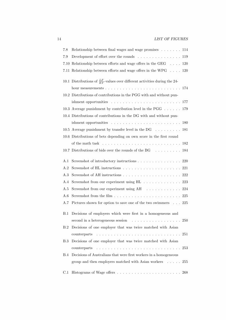
14 LIST OF FIGURES
7.8 Relationship between final wages and wage promises . . . . . . . 114
7.9 Development of effort over the rounds . . . . . . . . . . . . . . . 119
7.10 Relationship between efforts and wage offers in the GEG . . . . 120
7.11 Relationship between efforts and wage offers in the WPG . . . . 120
10.1 Distributions of LFHF -values over different activities during the 24-
hour measurements . . . . . . . . . . . . . . . . . . . . . . . . . . 174
10.2 Distributions of contributions in the PGG with and without pun-
ishment opportunities . . . . . . . . . . . . . . . . . . . . . . . . 177
10.3 Average punishment by contribution level in the PGG . . . . . . 179
10.4 Distributions of contributions in the DG with and without pun-
ishment opportunities . . . . . . . . . . . . . . . . . . . . . . . . 180
10.5 Average punishment by transfer level in the DG . . . . . . . . . 181
10.6 Distributions of bets depending on own score in the first round
of the math task . . . . . . . . . . . . . . . . . . . . . . . . . . . 182
10.7 Distributions of bids over the rounds of the BG . . . . . . . . . 184
A.1 Screenshot of introductory instructions . . . . . . . . . . . . . . . 220
A.2 Screenshot of HL instructions . . . . . . . . . . . . . . . . . . . . 221
A.3 Screenshot of AH instructions . . . . . . . . . . . . . . . . . . . . 222
A.4 Screenshot from our experiment using HL . . . . . . . . . . . . . 223
A.5 Screenshot from our experiment using AH . . . . . . . . . . . . 224
A.6 Screenshot from the film . . . . . . . . . . . . . . . . . . . . . . . 225
A.7 Pictures shown for option to save one of the two swimmers . . . 225
B.1 Decisions of employers which were first in a homogeneous and
second in a heterogeneous session . . . . . . . . . . . . . . . . . 250
B.2 Decisions of one employer that was twice matched with Asian
counterparts . . . . . . . . . . . . . . . . . . . . . . . . . . . . . 251
B.3 Decisions of one employer that was twice matched with Asian
counterparts . . . . . . . . . . . . . . . . . . . . . . . . . . . . . 253
B.4 Decisions of Australians that were first workers in a homogeneous
group and then employers matched with Asian workers . . . . . 255
C.1 Histograms of Wage offers . . . . . . . . . . . . . . . . . . . . . . 268

LIST OF FIGURES 15
C.2 Histograms of returned efforts . . . . . . . . . . . . . . . . . . . . 269
C.3 Histogram of final wages . . . . . . . . . . . . . . . . . . . . . . . 270
C.4 Simplified reaction patterns . . . . . . . . . . . . . . . . . . . . . 270
C.5 Development of average decisions during the games . . . . . . . . 271
E.1 The QRS complex in a typical heart rate signal . . . . . . . . . . 298

16 LIST OF FIGURES
Abbreviations
Table 1: List of abbreviations
AH Risk elicitation method by Andreoni and Harbaugh (2009)BDM Becker-DeGroot-Marschak mechanism by Becker et al. (1964)BG Bidding gameCRB Convex risk budgetDG Dictator gameECG ElectrocardiogramEG Risk elicitation method by Eckel and Grossman (2002)EUT Expected utility theoryGEG Gift exchange gameHF High frequencyHL Risk elicitation method by Holt and Laury (2002)HO Risk elicitation method by Hey and Orme (1994)HRV Heart rate variabilityLF Low frequencyMPL Multiple price listMSP Multiple switching pointsPGG Public good gamePT Prospect theoryRDU Rank-dependent utility theorySSP Single switching pointWPG Wage promising game
LIST OF FIGURES 17
Acknowledgements
While the compilation of a PhD thesis is primarily a significant individual task,
starting on a topic and progressing towards becoming a specialist in a field is
seldom an exclusively private accomplishment. For this reason I would like to
thank many of those that helped me embark onto, and finish the PhD journey,
by providing financial resources, subject-related and personal advice.
Financially, the research included in the following chapters has received mon-
etary support from Uwe Dulleck, Cameron Newton, Benno Torgler and Andrea
Ristl through their Australian Research Council Linkage Grant LP0884074 “Us-
ing Heart Rate Variability measurements to identify the effects of stress on de-
cision making” to conduct the economic experiments and to cover travel costs
to visit collaborators and conferences. Further financial support has been re-
ceived from the QUT School of Economics and Finance, for travel costs, con-
ferences and budgets that made economic experiments feasible. Furthermore,
much of the computational and storage resources were provided by QUT’s high-
performance computing group (HPC) services without which large parts of the
data analysis would have been infeasible. Additional funding has been re-
ceived from QUT’s international office, enabling me to collaborate with other
researchers around the globe. Further financial support has also been received
by Southeast University (Nanjing, China). I am very thankful for this support,
which made the research presented in this thesis possible.
I am also grateful for the support of other researchers, providing their valu-
able opinions on various parts of the projects. I received helpful comments and
profited from discussions during presentations at seminars at Southeast Univer-
sity in Nanjing, the University of Innsbruck, the University of Oviedo, and the
GATE at the University of Lyon. Furthermore, I advanced due to feedback re-
ceived at the following conferences. The ANZWEE 2010 in Sydney and 2011 in
Melbourne; the WEAI 2011 in Brisbane; the ESAM 2011 in Adelaide; the ACE
2011 in Canberra; the SWSEE 2011 in Sydney; the Australian PhD conference
2012 in Brisbane; the APESA 2012 in Xiamen; the Workshop in Behavioural
Economics 2012 in Brisbane; the THEEM 2012 in Kreuzlingen; the P&E Dok-
torandenforum 2012 in Zurich; and the ESEM 2012 in Malaga. Furthermore,

18 LIST OF FIGURES
helpful comments were also resulting form the QUT research colloquia 2010 and
2011.
Additional to this group feedback the work included in here also received
helpful comments and advice in personal communication from Mohammed Ab-
dellaoui, Simon Gachter, Pablo Guillen, Gigi Foster, Dirk Engelmann, David
Johnston, Rudolph Kerschbamer, Martin Kocher, David Matesanz, Xing Meng,
Cameron Newton, Nikos Nikiforakis, Lionel Page, Andrea Ristl and her team at
Autonom Talent, Markus Schaffner, Ulrich Schmidt, Bob Slonim, Marie-Claire
Villeval and Rudolf Winter-Ebmer as well as from three anonymous referee re-
ports.
I also would like to thank my principal supervisors Uwe Dulleck and Benno
Torgler who - additionally to their comments - helped to motivate and focus
my work which has now merged into this thesis. Special thanks also has to go
to Markus Schaffner who with his knowledge and willingness to give advice has
significantly contributed to my ability to finish this thesis. Additionally, I would
like to thank my fellow students at QUT for a very collaborative atmosphere,
enabling my to develop ideas and intergrate them into a joint thesis. I also
thank Tony Beatton, Ben Clapperton, Daniel Muller, Dave Savage and Juliana
Silva Goncalves for going through earlier versions of this work. Additionally, I
am thankful for research assistance work that I drew on in the course of this
thesis, particularly by Jessica Hay and George Li, but also of others who were
often available with helping hands.
Finally, I would like to acknowledge the work which has been done by others
in the projects which the chapters included in this thesis describe. For the study
in chapter 3 this have been Jacob Fell and Uwe Dulleck, for chapter 4 Markus
Schaffner, for chapter 7 Tony Beatton, Uwe Dulleck and Markus Schaffner, and
for chapter 8 Uwe Dulleck and Yumei He.
I would like to thank all these mentioned here and others who have helped
and supported me during this PhD journey with topic-related and personal
advice. A great thank you also goes to my parents Insa Fooken and Pit Wahl
who supported my academic development over a period of more than 10 years.
This support has been essential for my ability to finalise my academic degrees
of which this thesis is my potentially last achievement as a student.

LIST OF FIGURES 19
Statement of Original Authorship
The work contained in this thesis has not been previously submitted to meet
requirements for an award at this or any other higher education institution. To
the best of my knowledge and belief, the thesis contains no material previously
published or written by another person except where due reference is made.
Signature:
Date:
QUT Verified Signature

20 LIST OF FIGURES
Abstract
This thesis advances the knowledge of behavioural economics on the importance
of individual characteristics such as gender, personality or culture for choices
relevant to labour and insurance markets. It does so using economic experi-
ments, survey tools and physiological data, collected in economic laboratories
and in the field. More specifically, this thesis includes 5 experimental economic
studies investigating individual-specific characteristics (gender, age, personal-
ity, cultural background) in decision-making influenced by risk attitudes and
social preferences. One of these characteristics is also the physiological state
of decision-makers, measured by heart rate variability (HRV), recorded while
choices are being made. The results of the thesis show that individual-specific
characteristics play an important role for choices affected by social preferences,
a finding only to a lesser degree observable for risk preferences. This observation
is confirmed both when looking at revealed choice behaviour under economic in-
centives and when studying (latent) physiological responses of decision-makers.
Chapter 1
Introduction
A major insight of behavioural economics is that it is crucial to study human
decision making and social interactions in order to understand how individuals
and markets make use of and allocate scarce resources. Behavioural economics,
a branch of economics interested in developing a more refined and descriptively
adequate model of the individual decision maker, has been developing and grow-
ing over the last decades (e.g. Camerer, 2003; Camerer et al., 2003, as some
milestones). Often research in this field has been motivated by the inadequacy
of an overly simplistic standard model to explain behaviour observable in ex-
periments.1 That is, experiments tried to test the predictive accuracy of (often
central) theoretical assumptions and in many cases found that decision patterns
observed could not be aligned with standard model assumptions. This made it
necessary to develop economic theory further.
Designing and conducting simple thought, field and classroom experiments
has always been in the toolbox of economists to improve their theories. The
increasingly easier possibility of collecting and analysing large datasets on ex-
perimental decisions, particularly in computer laboratories through improved
IT infrastructure, has led to a rise of research in behavioural economic lab-
oratory experiments (see e.g. Friedman and Sunder, 1994; Roth and Kagel,
1995; Plott, 2008; Guala, 2005, for the recent development of methodology and
1What constitutes the standard, or most popular model is usually dynamic, but manybehavioural economic approaches have been triggered by observations that were not consistentwith the most commonly used model assumptions at the time of their development.
1

2 CHAPTER 1. INTRODUCTION
central results in experimental economics). Therefore, behavioural and experi-
mental economics are today closely linked, although neither is just a subset of
the other. Hence, differences exist between behavioural and experimental eco-
nomics, as behavioural economists also use observational datasets and do the-
oretical work. Conversely, non-behavioural experiments aim at understanding
only market-level outcomes. Furthermore, somewhat intermediary experiments
exist; for example, some experiments study behaviour based on assumptions
that are part of – or the core of – standard theory, some investigate the scope
of their applicability or quantify and find parameters for theoretical functional
forms of utility functions. Despite the fact that experimental and behavioural
economics are two separate fields with some overlap, much of the behavioural
economic research is motivated by experimental results and most experimental
studies investigate individual behaviour on a subject-specific or aggregate ba-
sis. Similarly, a large part of progress in behavioural economics is driven by
experimental results.
But what is the goal of behavioural economics, besides satisfying the intel-
lectual curiosity about wanting to learn about human decision making? And
what can economists learn more generally from empirically-driven experimental
approaches? Confirming specific theoretical assumptions does not validate a
theory and disproving them is not useful if there is no new, usable alternative
theoretical framework superior to the old one. Just knowing that part of a theory
is incorrect does not render the whole theory wrong. As most economists would
probably agree, their theories and models do not match some transcendental
and unobserved truth, but are useful tools for understanding and analysing re-
ality, for making predictions about observable phenomena in the world and,
arguably, to provide some normative advice. For example, in macroeconomics
many researchers would most likely agree that basically all assumptions of their
models are extremely simplistic and wrong in most specific cases but useful
for understanding aggregate behaviour. Similarly, in microeconomics incorrect
assumptions might be adequate if they are not too far from reality, if these devi-
ations from reality do not lead to unrealistic results, if they facilitate analysing
observed behaviour or if there is no usable and more accurate alternative at
hand.
3
An answer by behavioural economists to this willingness of being tolerant
towards some failures of the standard model is to search not just for single vio-
lations of theoretical assumptions, but patterns of behaviour not conforming to
theory. These patterns can be used to improve economic theories and models,
or to have a better working hypothesis and framework of thinking at hand us-
able for predictions.2 So far, three main modifications of the (most simplistic)
standard model based on such patterns have become more established, due to
the frequency of their observation, but also because of their empirical relevance
when making predictions. These can broadly be categorised as time, risk and
social preferences. Time preferences address the topic that individuals discount
outcomes in a non-continuous way depending on whether receiving these out-
comes occurs in the near or the far future. Risk (and uncertainty) preferences
take account of the fact that in the presence of probabilities (or likelihood lev-
els), individuals change their behavioural patterns compared to decision-making
with certain outcomes. Social preferences are used to explain why decision mak-
ers do not only care about their own outcomes, but also about the outcomes of
others.
These three types of behavioural preferences are by now widely accepted,
such that they have themselves become standard assumptions. This is par-
ticularly true for risk preferences, which have been discussed in the economic
literature for decades and further draw on a large research tradition in psychol-
ogy.3 Indeed, the existence of these three preference types (time, risk and social)
is often not investigated itself anymore, but it is studied under which conditions
behavioural preferences play a role and if it is possible to derive parameter es-
timates for them. Experimental techniques are the main way to study these
preferences and get a better picture about their applicability.
In the following thesis I will present 5 experimental studies that investigate
two of these elements. The first two of these, which are included in Part I,
investigate the measurement and determinants of risk attitudes. For this, the
2I refer to intermediary models that might not be a comprehensive and consistent theoryyet, but which help to develop and refine such a new, more comprehensive paradigm, asworking hypotheses or frameworks of thinking.
3For example, one might view expected utility theory as a core element of standard theoryand only the presence of probability weighting and reference-dependence as truly behaviouraleconomic theory, although both have been developed as a response to behavioural findingswhich could not be made sense of simply using expected value theory.

4 CHAPTER 1. INTRODUCTION
first study compares the results of two different elicitation methods of risk at-
titudes and uses experimental findings to evaluate what these methods can be
used for in other applications. The second study employs a similar framework
and adds personality measures and physiological data to risk attitude estimates
to investigate further sources and determinants of risk attitudes.
Part II continues with two studies that investigate determinants of social
preferences in an experimental labour market. In the first study of Part II
interaction between Australian and Asian students is studied. The second study
investigates attitudes towards inner-Chinese migrants and interaction between
groups of local and migrant workers.
Part III consists of one study that links decisions in a laboratory experiment
with activities outside of the laboratory. To do so, physiological measures are
used as a relevance indicator to compare the experiment to normal-day activities
and a university exam.4 In the experiment, social preferences and risk-taking
are studied, allowing to link and join Parts I and II.
The different studies and the Parts are, additional to all being behavioural
economic experiments, linked by two main factors. The first is that they all
are affected by and address the importance of individual characteristics in ex-
perimental decisions. Studying the importance of individual characteristics is
a central aspect for behavioural economists, although this aspect is often not
studied as a research agenda per se, but just one major underlying factor, al-
though studies directly investigating individual heterogeneity also exist (for ex-
ample Andrew Luccasen, 2012; Burlando and Guala, 2005). As such, a large
number of approaches study individual characteristics as a major factor de-
termining time, risk and social preferences as mainly co-varying factors or as
treatments. Examples are culture (Roth et al., 1991; Henrich, 2000; Henrich
et al., 2001), personality (Schmitt et al., 2008) or demographics such as gender
and age (Camerer, 2003, p.63-67). Indeed, the importance of individual-specific
factors is a central prerequisite for some behavioural economic research that tries
to get a better understanding of the foundations of certain preference types; for
example, research studying biological determinants of decision making such as
variations in decisions based on genes (e.g. Wallace et al., 2007; Cesarini et al.,
4The meaning of relevance is discussed in further detail in the context of this study.
5
2008) or on hormone levels (e.g. Zak et al., 2007; Crockett et al., 2010) strongly
relies on the fact that differences on the individual level matter for decisions.
However, the importance of individual characteristics is not only important
from the point of view of academic interest, but also if one wants to gener-
alise from experimental results: To interpret experimental findings in a wider
context, they have to contribute to understanding why individuals in the ex-
periment decided in a certain way, if general behavioural patterns are visible
(independent of the individuals studied), if and to what extend socialisation
and learning play a role or if behaviour is inherited (hence to what extend
observations are linked to the specific individual observed), and if institutions
can change certain preference types. Particularly the last factor is central for
policy-makers who are facing, but also influencing decisions of a – potentially
heterogeneous – population. These policy-makers need to know what leads to
more or less pronounced manifestations of certain preferences and which types
of individuals tend to have certain preferences patterns (more or less strongly)
to implement reasonable and effective policies. Therefore, understanding the
individual level is not only academically interesting, allowing to develop more
accurate theories, but also directly relevant for economic policy.
The second innovation in this thesis is the use of physiological data which
aims to make decisions comparable across different types of attitudes and to
out-of-laboratory events using objective data. Objective data has increasingly
been used in research using neuroscientific tools (Glimcher et al., 2008; Egidi
et al., 2008), and is a burgeoning field of research in economics (see further
below for a more detailed motivation of the specific data used in the studies
included in this thesis).
The following three sections introduce a framework of thinking which will
be referred to throughout the thesis to outline the understanding of individual-
specific characteristics. Furthermore, some background information on the intu-
ition of using physiological data is presented as it is essential for understanding
different Parts of the thesis.

6 CHAPTER 1. INTRODUCTION
1.1 Individual characteristics
Besides determining different types of behavioural preferences, another major
insight of behavioural economics is that individuals might differ in their time,
risk and social preferences. This insight can be summarised in the following sim-
ple framework of thinking in which a decision maker chooses between different
options in a way that can be made sense of with the following utility function:
Uit(p,Xi, Xj) =
∞∑t=1
k∑z=1
δtiwi(pz) (Vi(Xit) +Oij(Xjt)) (1.1)
Hence, decision maker i derives utility from the time-discounted (with 0 <
δti < 1 – preference for sooner to later) outcomes for himself (Xit) and for
others (Xjt) at times t and subject to the probability p of their occurrence.
Hence, the decision maker might value outcomes depending on whether they
will be consumed by him (Vi(·)), by others (Oij(·)) and depending on their
probability pz to be realised in state z (this probability might potentially be
weighted through wi(·)).5
Throughout this thesis, I will investigate several aspects of individual be-
haviour which can be understood in such a framework. However, I will drop the
time dimension and only study attitudes under risk and social attitudes.6 I will
come back to this framework and simplify or refine the framework depending
on the aspect under investigation. For example, such refinements make sense
when thinking about the shape or determinants of Vi(·), Oij(·) or wi(·). That is
in Part I, I will only study individual decision making, leaving out the dimen-
sion of Oij(·), and focus on situations for which I assume wi(p) = p, while only
including a small extension on probability weighting. In Part II I will focus on
decisions that are affected by social preferences. For this, I will further refine the
role of Vi(Xi) and Oij(Xj).7 In the last Part III I will include both dimensions
parallel to each other. I will return to the framework of thinking and provide
more detail in the respective Parts.
5The decision maker chooses by maximizing his utility given the budget constraint in statez ∈ [1, . . . , k] s.t. Xiz +Xjz ≤ Xz with Xz = the total amount in the opportunity set of i.
6Further including the time dimension is interesting but beyond the scope of this thesis.7Here and later Vi(·) and Oij(·) are described as additive, which is not a necessity. However,
as the framework in this thesis has only an illustrative purpose and as the additivity illustratesthe separability assumed about Vi(·) and Oij(·), this form is used throughout.

1.2. WHYNEUROSCIENTIFIC AND PHYSIOLOGICALMEASUREMENTS?7
1.2 Why neuroscientific and physiological mea-
surements?
Researchers in behavioural economics are interested in individual decision mak-
ing. However, as a professional economist interested in quantifiable outcomes,
why should one care about the neural or physiological process underlying de-
cisions? Why not stop with observed (or revealed) choices in experiments and
reality and simply study these? Economists are mainly concerned about how
individuals make decisions over scarce resources and observed choices should
be sufficient for understanding the tangible and economically relevant part of
decision making.
However, the approach of most behavioural economists goes further. They
want to improve the level of explanation of the decision making process and
understand how individuals make decisions. The belief behind this is that the-
oretical concepts should have more than just abstract meaning, but relate to
psychological and other potentially latent processes within the decision maker.
The belief is hence that this will eventually increase the relevance of theory in
explaining the natural foundation of reality and the goal is to understand the
full process of decision making. For this behavioural economists aim to check
if the theoretical concepts used in economic analysis have some correspondence
in neural or physiological processes (see e.g. Egidi et al., 2008). This notion has
led to the field of neuroeconomics, which mainly studies brain activity (with
brain scanners), but also physiological responses to stimuli that are not under
the conscious control of the decision maker. Examples for such physiological re-
sponses are facial expressions, sweating (measuring skin conductance) or heart
activity (using electrocardiograms) that parallel certain parts of the decision
process (see Camerer et al., 2005, for an introduction).
The goal of neuroeconomics is, as I see it (others may or may not agree),
not to prove or disprove theories, but exploratory in its nature. Hence, it can
help to point research into promising directions and provide some reality check
by adding objective information. However, as it uses research tools that are not
developed for testing economic theories, it always has to speak from outside to
economists and there is no direct causal link between neurological or physiolog-

8 CHAPTER 1. INTRODUCTION
ical measures and observed choice behaviour. These two data points just occur
at the same point in time and this fact is then interpreted such that they are
related, a procedure known as reverse inference.8 Additionally, a theoretical
dimension usually based on a neuroscientific understanding of decision-making
is added to the joint occurrence of the data to provide an indirect causal link.
As a result a neuroeconomic research agenda can at best help to detect a
neural basis of economic decisions, for example when detecting brain regions
that are active during social decisions making. Adding neural or physiological
data as an objective measure can help to put experimental decisions into a
broader perspective. For example, it can help to understand how important
experimental measurements are compared to other decisions inside and outside
the laboratory such as understanding experimental monetary gains on a scale
of positive emotional reactions. As such, physiological measurements could take
a role of shadow values or a relevance detector, similar to the role of using real
monetary stakes that depend on choices made in economic experiments. As such
it follows psychological research that uses physiological signals as psychological
indicators (e.g. Cacioppo and Tassinary, 1990; Rohrmann and Hopp, 2008) and
research on the intersection of economics and psychology which uses neural
markers as indicators for experienced values (O’Doherty, 2004; Knoch et al.,
2010) in the sense of Uit(·) in the framework described above.
In this sense I will use data on heart rate variability (HRV) of experimental
participants in Parts I and III, assuming that HRV measures potentially re-
flect Ui(·) as described above. In order to facilitate the understanding of these
sections the following section describes HRV in terms of measuring the physi-
ological state of an individual during the decisions making process. Although
itself not deductive, this section should also provide a link for why HRV and
economic decisions are potentially causally related.
8Reverse inference refers to the approach of measuring the paralleling development of twodata generating processes and interpreting joint development as causally related. Using reverseinference in neuroeconomic research is common, but not unproblematic (see e.g. Phelps, 2009,for a discussion).

1.3. HEART RATE VARIABILITY MEASUREMENT 9
1.3 Heart rate variability measurement
HRV describes changes in the heart rate over time. To measure HRV, usually
Electrocardiograms (ECGs) with numerous electrodes are used as signal detec-
tors. For the studies described in this thesis portable ECG Recorders (AR12)
with 3 electrodes attached to a participant’s chest were used to collect data on
the temporal succession of heart beats. From the recorded ECG the heart rate
as well as the heart rate variability for a given period is calculated. Here heart
rate measurements of participants over the entire course of the experiment is
used to determine their HRV in a succession of 5 second intervals, which are
averaged over the decision time investigated in the analysis.
HRV as a physiological indicator is mainly used in medical research (Camm
et al., 1996) and has been linked to psychological, emotional and mental states.
Interpretations of HRV measures mainly rest on the understanding that the au-
tonomous nervous system (ANS) is influenced by the sympathetic and parasym-
pathetic systems and that the influence of the two systems is reflected in the
heart rate (see Breedlove et al., 2010, for some general discussion of physio-
logical processes).9 The sympathetic system is responsible for fight-or-flight
responses, using sympathetic nerves and hormones (particularly adrenaline).
The parasympathetic system controls rest and relaxation through specific pace-
maker cells. While both systems are constantly active parallel to each other,
the degree to which one of the systems controls the heart rate in a given period
varies.
The two systems operate at different speeds. Changes in the heart rate due to
increased sympathetic activity have a longer time horizon compared to parasym-
pathetic activity.10 This allows for a decomposition of the heart rate into differ-
ent frequencies, with varying importance of sympathetic and parasympathetic
activity. Practically, this is done in estimation procedures using waves of differ-
ent lengths (different frequencies). Using decompositions into frequencies and
studying their relative influence (power) at a given time allows identification
9Other systems are active alongside, regulating respiration, body temperature and bloodpressure. The influence of these other systems is eliminated from the data before using HRVmeasures.
10Increases in sympathetic activity have their strongest effect after more than 5 second whileincreases in parasympathetic activity have their strongest effect after less than 5 seconds.

10 CHAPTER 1. INTRODUCTION
of the effect of the sympathetic and the parasympathetic system, reduces some
of individual heterogeneity in heart rate data and makes comparisons across
individuals possible.11
The ratio of the low frequency (LF, .033-.15 Hz) to the high frequency (HF,
.15-.4 Hz) mirrors the activity of sympathetic to parasympathetic activity (see
Malik, 2007). The LFHF ratio serves as an indicator of psychologically induced
physiological stress (see Appelhans and Luecken, 2006, who also include more
detail on how HRV measures are determined). In a laboratory environment
this indicator conveys information about psychological states (Berntson and
Cacioppo, 2008); for example, a higher ratio of sympathetic to parasympathetic
activity has been connected to increased mental stress (Berntson et al., 1994).
As these mental factors can play a decisive role in economic decision making,
studying a connection between economically important choices and HRV ap-
pears meaningful.
While the economic literature that uses HRV is still small, studies have been
conducted in the context of gambling (Meyer et al., 2000; Wulfert et al., 2005),
on perceptions of “unfair”payments (Falk et al., 2011), stress when being made
accountable for decisions (Brandts and Garofalo, 2011), time preferences (Daly
et al., 2009) and tax compliance (Dulleck et al., 2012b). Dulleck et al. (2011b)
provide general guidelines on linking economic experiments and HRV data.
11More information on the estimation procedures used for the studies is included in thetechnical appendix.

Part I
Consistency and sources of
individual risk attitudes
11

Chapter 2
Individual risk attitudes
2.1 Introduction
Understanding decision making under risk is a major and important topic in
economics due to its far-reaching consequences for individual, organisational
and policy choices and for understanding how particular market outcomes come
about. In this chapter, I try to contribute to this understanding of risk atti-
tudes by presenting two studies. In the first study I investigate the usefulness of
estimated risk aversion parameters from two experimental risk elicitation meth-
ods. I do so by asking how much information the resulting values can provide
and what they can be used for to make risk attitude statements about groups
of experimental participants and individuals. In the second study I investigate
potential sources of risk aversion, its physiological basis and its connection to
decision making in a dilemma with limited time.
But what does decision making under risk mean? Broadly speaking, individ-
uals decide under risk when they face outcomes that depend on probabilities or
when different choice options have differing (known) variances. Individuals are
confronted with such risky choices in various aspects of daily life, for example
in financial investments, when gambling, choosing job and business strategies,
or when setting their consumption and investment levels.
When trying to define attitudes towards risk on a more formal level, it
is useful to consider different decision rules that could guide decisions when
13

14 CHAPTER 2. RIST ATTITUDES INTRODUCTION
deciding over probabilistic outcomes.1 A first benchmark for risk attitudes is to
assume that individuals make choices providing the highest pay-off in terms of
their expected value (see for example Samuelson, 1938, for an early discussion).
If choosing options with the highest value would be an individual’s choice rule,
he or she would make decisions that give the highest expected value for
EVi =
k∑z=1
pz ·Xiz. (2.1)
Hence, under such a choice rule, when facing several risky options, outcomes
are simply weighted by their probability of occurrence. If an individual decides
based on the expected value of choice options, this is usually referred to as a
risk neutral attitude, and provides a benchmark for other, alternative decision
rules.
Preferring choice options with a smaller (larger) variance compared to the
risk neutral option and being willing to give up expected value for this implies
risk aversion (loving). In reality, and in many domains of economically relevant
decision making it is often observed that (on average) individuals are risk averse,
although there usually is some noticeable heterogeneity in risk attitudes between
individuals, showing different degrees of risk aversion, risk neutrality and loving
for different risky options.
In order to make sense of this empirical finding, economists have used ex-
pected utility theory (EUT) to model risk averse behaviour (see Stigler, 1950a,b,
for an early discussion of utility theory). Hence, EUT stems from behavioural
findings although today most behavioural economists tend to view EUT as too
simplistic and with an insufficient descriptive accuracy. For this reason, more
refined models, such as rank-dependent utility theory (RDU) and prospect the-
ory (PT) are increasingly popular.2 However, since much of the experimental
1There are a number of approaches to define risk attitudes without relying on functionalforms of utility functions. However, here I will focus on measures of risk attitudes based onfunctional forms.
2See Wakker (2010) for a detailed discussion of more advanced theories. These moreadvanced theories take account of the fact that specifications of the utility function for anindividual can be reference-dependent, particularly when comparing the utility from gains tothe one from losses. They are also able to capture how individuals transform probabilities, i.e.mainly through probability weighting functions where w(p) 6= p in the sense of the frameworkof thinking described in the introduction. Under these theories, the understanding of riskattitudes can be more complicated (potentially richer) then under EUT.

2.1. INTRODUCTION 15
literature still relies on EUT, in particular the literature that aims to go be-
yond the study of risk attitudes themselves and that tries to link experimental
measures on risk attitudes to other domains of decisions making, such as social
preferences or choices outside of the laboratory, the main part of the following
two chapters will focus on EUT and add only one small excursion on non-EUT
interpretations in the second chapter.3 The reason for this is - besides mak-
ing the studies comparable to the literature - that the data was collected with
methods designed for eliciting risk attitudes under this paradigm, making them
partly unsuitable and unreasonable for analysis that interprets decisions under
a more advanced paradigm. Furthermore, as visible in the small extension that
incorporated probability weighting, in the more advanced framework interpre-
tations of experimental results in terms of risk attitudes become more difficult.
The reason for this is that simple interpretations of risk attitudes are mainly
meaningful under an EUT framework and do not have the same one-dimensional
correspondence in other theories.
In order to understand the measures of risk elicitation used in the two stud-
ies of this Part, it is useful to recall some central elements of the EUT frame-
work. As mentioned above, EUT was mainly developed as a response to the
behavioural finding that individuals often do not decide based on the expected
value of risky outcomes (see Bernoulli, 1954, for a first introduction to EUT).
More formally said, for many individuals
E[Ui(p,Xi)] 6=k∑z=1
pz ·Xiz. (2.2)
The notion that most individuals are somewhat risk averse can be captured
with EUT, which incorporated the notion of decreasing marginal utility for
higher monetary outcomes. In other words this implies the (intuitively and
empirically confirmed) notion that the gain in utility from one extra dollar is
greater when having nothing than when having one hundred dollars already.
3The extension will allow for subjective probabilities which are weighted by the decision-maker such that objective probabilities have to be treated differently than subjective prob-abilities. Quiggin (1982) and Schmeidler (1989) developed theoretical approaches to modelthis behaviour. Practically, in the analysis this probability transformation is taken accountof by using a probability weighting function as described by Prelec (1998). See also Gonzalezand Wu (1999) for a discussion of the shape of the weighting function.

16 CHAPTER 2. RIST ATTITUDES INTRODUCTION
One could express this in the formal framework of thinking as
Ui(p,Xi) =
k∑z=1
pzVi(Xiz) (2.3)
with the common assumptions of ∂V (Xi)∂Xi
> 0 and ∂2V (Xi)∂X2
i< 0, the second
of which implies risk aversion. However, the EUT framework also allows for
heterogeneity of individuals, and so risk loving individuals with ∂2V (Xi)∂X2
i> 0 or
risk neutral individuals with ∂2V (Xi)∂X2
i= 0 might also be present in the population
studied.
Indeed, through the popularity of EUT, not least since its formalisation
by von Neumann and Morgenstern (1944), thinking about risk aversion on a
relatively simple and unique scale, identifying different degrees of risk averse,
risk neutral and risk loving individuals, is integrally linked to EUT, particularly
in theoretical terms.4 For example, the so-called Arrow-Pratt coefficients of risk
aversion (named after the work by Pratt, 1964; Arrow, 1971), which are also used
in the analysis in the following chapters, allow for a theoretically straightforward
and simple understanding of risk attitudes (see also Varian, 1992; Mas-Colell
et al., 1995, for a textbook discussion). Hence, assuming a certain functional
form of utility functions, individuals can be classified in terms of risk aversion
according to a simple parameter.
Building on these frameworks of EUT and the use of Arrow-Pratt coeffi-
cients, many experimental elicitation methods of risk attitudes assume simple
utility functions of the form Vi(Xi) = Xαii that imply constant relative risk
aversion (CRRA) for individual i, as in this framework the curvature of the
utility function αi is a direct measure of individual risk aversion. Given such
a utility function the Arrow-Pratt coefficient of relative risk aversion can be
calculated as
Ri(X) = −V′′(X) ·XV ′(X)
= −αi · (αi − 1) ·Xαi−2X
αiXαi−1= 1− αi (2.4)
4In most descriptively more advanced theories on decision making under risk and uncer-tainty it is still possible to talk about risk attitudes, but usually in these frameworks individualscan be both risk averse and risk loving, depending on the reference point or the likelihoodlevel of the decision. Under EUT, an individual is usually either risk averse or risk loving andat least this judgement is independent of the likelihood level .

2.1. INTRODUCTION 17
and∂Ri(X)
∂X= 0→ constant (2.5)
This coefficient allows for a simple interpretation. If αi > 1, Ri(X) < 0,
hence the individual is risk loving; if αi = 1, he is risk neutral; and if αi < 1,
he is risk averse. As a result, risk elicitation methods with which αi can be de-
termined have been the workhorse in large parts of the experimental economic
literature, particularly when trying to find measures that can be used in empir-
ical research designs in which risk attitudes are just one of several elements of
interest. Conversely, when just investigating risk attitudes, non-EUT functions
and non-parametric analysis are also frequently used.
2.1.1 Aims of the following chapters
Given the importance of risk attitudes in daily decision making for individuals,
organisations, policy makers and market outcomes, understanding risk attitudes
is not only a central topic for theorists, but also for empirical researchers. In
the following two chapters I will investigate two aspects in more detail, both
aimed at getting a better understanding of risk attitudes, how they can be
elicited in the lab and how their measured parameter values can be interpreted.
Following the main theme of this thesis, they will also be evaluated considering
the question of heterogeneity between individuals.
More specifically, the following chapter investigates the stability of two dif-
ferent risk elicitation measures from the perspective of their usability for further
research. That is, in this first study the consistency of choices in two methods
used to elicit EUT-based risk preferences is compared on an aggregate as well
as on an individual level. In the experiment subjects choose twice from a list
of nine decisions between two lotteries, as introduced by Holt and Laury (2002,
2005, HL). The HL method is by now the probably most popular method to
elicit risk attitudes. Decisions in the HL method alternate with decisions us-
ing the budget approach introduced by Andreoni and Harbaugh (2009, AH).
While results show that on an aggregate (subject pool) level the results within
each method are consistent, they provide different aggregate results between
the methods. That is, the distribution of risk attitudes is the same over the

18 CHAPTER 2. RIST ATTITUDES INTRODUCTION
two rounds for each method. However, the distributions of the two methods
differ from one another. Furthermore, on an individual (within-subject) level,
behaviour is far from consistent. Within each method as well as across meth-
ods low correlations of the estimated risk aversion coefficients of αi (assuming
Vi(Xi) = Xαii ) are observed, and even low correlations of ordered rankings of
risk attitudes between individuals are detected. This indicates that it is difficult
to elicit values of utility functions that are easily interpretable in an EUT frame-
work and illustrates the difficulty when aiming to use experimental measures
on risk attitudes for linking them to other decision patterns in experimental or
observational data.
The second chapter in this Part tries to improve the understanding of deci-
sion making more generally, as well as the results from the first chapter specif-
ically, adding psychological and physiological data to the measures of the risk
elicitation methods which were already used in the preceding chapter. Using
this additional data, the difference in the results of the two risk elicitation meth-
ods is further investigated by linking estimates of risk attitudes to gender, age,
personality traits, a decision in a dilemma, and physiological states – as mea-
sured by heart rate variability (HRV). The results of this study indicate that
differences between the two elicitation methods can partly be explained by gen-
der, but not by personality traits. Furthermore, HRV is linked to risk-taking in
the experiment for at least one of the methods, indicating that more stressed
individuals display more risk aversion. Finally, risk attitudes are not predictive
for the ability to decide in a dilemma, but personality traits are. Surprisingly,
there is also no apparent relationship between the physiological state during
the dilemma situation and the ability to make a decision. These are interesting
results for policy-makers, but also for personnel managers who have to decide
on incentives that are affecting certain types of people or who have to nominate
individuals for jobs that are characterised by risky environments where decisions
have to be taken relatively quickly.
As the same risk elicitation methods were used in both studies, I proceed
with giving a brief description of the two methods, as understanding them and
their connection is equally important for both studies. In the following two
studies, consequently, only information about the procedural implementation of

2.2. RISK ELICITATION METHODS 19
the methods into the experimental protocol is included.
2.2 Risk elicitation methods
In reality many decisions are taken where choices do not lead to outcomes pre-
dictable with certainty, but are leading to probabilistic realisations. Economists
usually refer to such situations as decisions under risk (or, more generally, under
uncertainty when including cases in which exact probabilities are not known).
As many individuals show different choice patterns when faced with risky out-
comes, it is important to have a good understanding of decision-making under
risk. For this reason elicitation of risk attitudes has been extensively discussed
in the experimental literature and various approaches have been proposed for
experimental risk elicitation. I will just mention central ones here to illustrate
the diversity of different options available, even when only focussing on methods
designed with an EUT framework in mind. For a more comprehensive discussion
of different methods of risk elicitation see Harrison and Rutstrom (2008). How-
ever, even the list included in their discussion could be further extended by more
recent approaches in this constantly evolving field. In the following description
I will therefore focus on the (in my perception) most popular methods.
One of the first methods used to elicit (EUT-based) risk attitudes in labora-
tory environments was the auction design method through the so-called Becker-
DeGroot-Marschak (BDM) mechanism (Becker et al., 1964). Early versions of
this method can be found in Harrison (1986, 1990). The basic idea of this
method is to use the selling behaviour in auctions as an experimental mea-
sure of risk aversion. The intuition behind the measure is that individuals will
strategically overstate selling prices to increase their payoffs. However, as over-
stating the selling price increases the risk of not selling at all, risk aversion will
limit such behaviour. While this procedure appears intuitive for professional
economists, the method has not become too popular amongst more empirical
oriented researchers and in the literature. One reason for this might be that
it is unclear if experimental participants understand this experimental set-up
similarly to the researchers, if they chose strategically only based on their risk
attitudes, or if they also make decisions based on some other (latent) heuristics.

20 CHAPTER 2. RIST ATTITUDES INTRODUCTION
Three other methods have become more popular that are also aimed at elic-
iting risk attitudes under EUT. One of these is the method used by Hey and
Orme (1994, HO) which sequentially presents subjects with a number of lottery
pairs that have varying combinations of probabilities and outcomes. These pair-
wise combinations of lotteries are usually presented in pie charts that illustrate
the probabilities and payoffs of the two lotteries in the pairwise choice.
The multiple price list (MPL) design also typically presents individuals pair-
wise (binary) choices between two options. However, in the “list”of lottery
choices, payoffs usually remain the same and only the corresponding proba-
bilities are varied when advancing to the next choice. The design by HL as
described in more detail below is by now probably the most popular version of
a MPL approach, and widely applied in the empirically oriented literature.
The third commonly used method is the approach by Eckel and Grossman
(2002, EG), in which experimental participants make decisions between differ-
ent options with fixed probabilities (usually p = .5 or p = 1, hence certainty
equivalents) and which varies the different outcomes that occur with a certain
probability or with certainty over a sequence of choices.5
While all these methods were designed with an EUT framework in mind,
they all differ somewhat in their choice variable or the experimenter’s treat-
ment variable. In the BDM procedure participants chose their selling prices; in
HO outcomes and probabilities change between periods; for HL only probabil-
ities change; and in EG probabilities remain constant and only payoffs change.
Hence, when looking at the comparability of EUT risk attitude measures these
might be different between methods because of their choice variables.
For the two methods studied in the following, this potential source of dif-
ferences in measured results is minimised by using two methods that are based
on the same choice variable, i.e. probabilities. Furthermore, the experimental
tasks were both designed with the same individual utility function of the form
Vi(Xi) = Xαii and EUT in mind. This allows to estimate risk attitudes for both
methods which can be directly compared between the two methods, based on
the Arrow-Pratt coefficient α.
The two methods used in the two studies included in this Part are the risk
5For example an individual would compare receiving 4 for certain to a first choice thatgives 0 or 10 with p = .5, a second choice that gives 2 or 8 with p = .5, and so on.
2.2. RISK ELICITATION METHODS 21
elicitation method by HL and a method by AH, which can be used to infer
CRRA coefficients representing risk attitudes. Both methods are described in
further detail below. In the implementation of the risk elicitation tasks the
experimental designs followed HL and AH closely. Instructions and screenshots
of the experiment can be found in the appendix. The implementation of the
two experiments was done similarly, and the common features are therefore
included in this introductory chapter. Some minor, more procedural details are
also included in the respective chapters describing the practical implementation
of the methods.
Procedurally, for both methods in the two experiments, a random incentive
mechanism with monetary incentives was used. This was done to avoid wealth
and portfolio-building effects in the two tasks. More specifically, one of two
rounds was randomly selected and from this round one randomly selected choice
of each method was determined for final payments. In both methods 2 rounds
with 9 choices for each method were played, alternating between methods. The
payoff structure for the two methods was designed such that the expected gain
for a risk neutral decision maker from the 18 decisions in each method was the
same across the two methods. This was done to increase their comparability,
which was particularly relevant for the analysis in the first study.
2.2.1 Holt and Laury Method
As mentioned before, HL used a MLP design which enabled them to easily
classify individuals into categories of risk aversion. It has become one of the most
popular elicitation methods. For the HL method, participants were able to see a
MPL and were asked to make choices separately for each row between a pair of
lotteries (see Table 2.1). The two lotteries each incorporate two outcomes, each
with a higher and a lower payoff. Both lotteries have the same probabilities
for the low and high option, but differing dispersions between the outcomes.
Hence, for each further decision row down, the probability mass on the higher
payoff increased by 10%, making the safer option A (i.e., the option with a
lower variance in payoffs) less attractive. The two studies included here deviate
from HL slightly by leaving out the certain option (i.e., 100% probability of the
higher payoff) to avoid any reference point of safety. This reduces the number
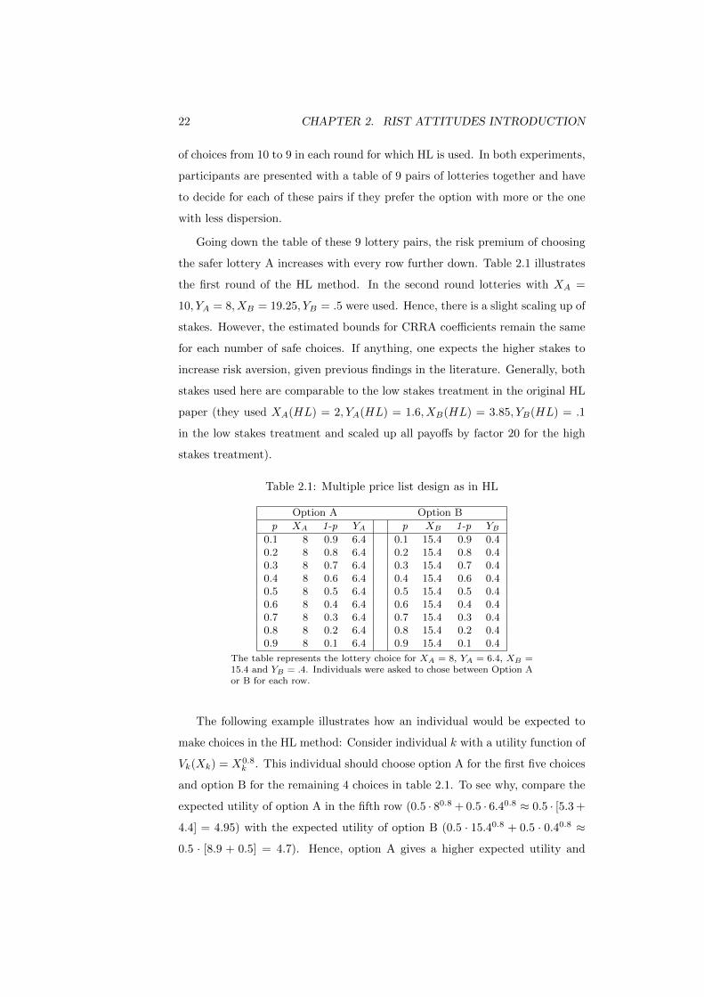
22 CHAPTER 2. RIST ATTITUDES INTRODUCTION
of choices from 10 to 9 in each round for which HL is used. In both experiments,
participants are presented with a table of 9 pairs of lotteries together and have
to decide for each of these pairs if they prefer the option with more or the one
with less dispersion.
Going down the table of these 9 lottery pairs, the risk premium of choosing
the safer lottery A increases with every row further down. Table 2.1 illustrates
the first round of the HL method. In the second round lotteries with XA =
10, YA = 8, XB = 19.25, YB = .5 were used. Hence, there is a slight scaling up of
stakes. However, the estimated bounds for CRRA coefficients remain the same
for each number of safe choices. If anything, one expects the higher stakes to
increase risk aversion, given previous findings in the literature. Generally, both
stakes used here are comparable to the low stakes treatment in the original HL
paper (they used XA(HL) = 2, YA(HL) = 1.6, XB(HL) = 3.85, YB(HL) = .1
in the low stakes treatment and scaled up all payoffs by factor 20 for the high
stakes treatment).
Table 2.1: Multiple price list design as in HL
Option A Option B
p XA 1-p YA p XB 1-p YB0.1 8 0.9 6.4 0.1 15.4 0.9 0.40.2 8 0.8 6.4 0.2 15.4 0.8 0.40.3 8 0.7 6.4 0.3 15.4 0.7 0.40.4 8 0.6 6.4 0.4 15.4 0.6 0.40.5 8 0.5 6.4 0.5 15.4 0.5 0.40.6 8 0.4 6.4 0.6 15.4 0.4 0.40.7 8 0.3 6.4 0.7 15.4 0.3 0.40.8 8 0.2 6.4 0.8 15.4 0.2 0.40.9 8 0.1 6.4 0.9 15.4 0.1 0.4
The table represents the lottery choice for XA = 8, YA = 6.4, XB =15.4 and YB = .4. Individuals were asked to chose between Option Aor B for each row.
The following example illustrates how an individual would be expected to
make choices in the HL method: Consider individual k with a utility function of
Vk(Xk) = X0.8k . This individual should choose option A for the first five choices
and option B for the remaining 4 choices in table 2.1. To see why, compare the
expected utility of option A in the fifth row (0.5 · 80.8 + 0.5 · 6.40.8 ≈ 0.5 · [5.3 +
4.4] = 4.95) with the expected utility of option B (0.5 · 15.40.8 + 0.5 · 0.40.8 ≈
0.5 · [8.9 + 0.5] = 4.7). Hence, option A gives a higher expected utility and
2.2. RISK ELICITATION METHODS 23
should consequently be preferred. Going one further decision row down, the
expected utility from option A is 4.94 (0.6 · 5.3 + 0.4 · 4.4) and from option B
5.54 (0.6 ·8.9+0.4 ·0.5), hence option B should be preferred. Furthermore, given
the utility function of Vj(Xj) = X0.8j , all choices before the fifth choice will be
in favour of option A, and after the fifth choice option B should be preferred,
as they provide a higher expected utility. Hence, given a utility function of the
form of Vi(Xi) = Xαii , individuals that make optimal choices should have a
single switching point (SSP) from option A to option B.
In their study, HL find that subjects are generally risk averse and that risk
aversion increases with the size of the stakes, a statement they refined in a
second study (Holt and Laury, 2005) replying to a comment by Harrison et al.
(2005b). Since it’s publication, HL’s method has been used in several studies
as it allows to determine risk premia that participants are willing to pay for
experimental lotteries. HL can also be used to infer CRRA coefficients. Due
to this (theoretically) straightforward design and its simplicity, HL enjoys a
high popularity in the economics literature. However, despite this simplicity,
experimental evidence reveals that subjects show behaviour inconsistent with
EUT, more specifically multiple switching points between option A (the option
with a lower variance) and option B (the option with a higher variance). This
may be interpreted as relatively broad bandwidths of possible risk premia -
including patterns of indifference between lotteries that make it unclear whether
individuals are risk loving or risk averse.
2.2.2 Andreoni and Harbaugh Method
The implementation of the AH risk elicitation method followed the original
approach, but deviated by not using lotteries involving losses. The method by
AH tries to elicit risk attitudes by letting participants allocate a (convex risk)
budget (CRB) between their probability of winning (prob) and the amount X
received in case of winning. Each extra percentage point of winning costs the
decision maker a certain price (price); hence, participants chose their preferred
prob∗ such that their winning amount will be X∗ = µ−prob∗ ·price with µ being
the maximum gain, or budget, that can be won with corresponding probµ = 0.
Table 2.2 includes the pairs of µ and price in the two rounds of the experiments.
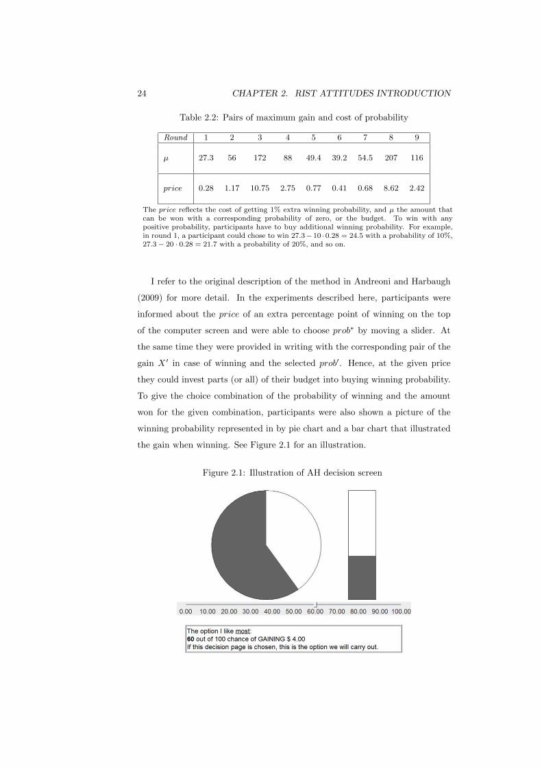
24 CHAPTER 2. RIST ATTITUDES INTRODUCTION
Table 2.2: Pairs of maximum gain and cost of probability
Round 1 2 3 4 5 6 7 8 9
µ 27.3 56 172 88 49.4 39.2 54.5 207 116
price 0.28 1.17 10.75 2.75 0.77 0.41 0.68 8.62 2.42
The price reflects the cost of getting 1% extra winning probability, and µ the amount thatcan be won with a corresponding probability of zero, or the budget. To win with anypositive probability, participants have to buy additional winning probability. For example,in round 1, a participant could chose to win 27.3−10 ·0.28 = 24.5 with a probability of 10%,27.3− 20 · 0.28 = 21.7 with a probability of 20%, and so on.
I refer to the original description of the method in Andreoni and Harbaugh
(2009) for more detail. In the experiments described here, participants were
informed about the price of an extra percentage point of winning on the top
of the computer screen and were able to choose prob∗ by moving a slider. At
the same time they were provided in writing with the corresponding pair of the
gain X ′ in case of winning and the selected prob′. Hence, at the given price
they could invest parts (or all) of their budget into buying winning probability.
To give the choice combination of the probability of winning and the amount
won for the given combination, participants were also shown a picture of the
winning probability represented in by pie chart and a bar chart that illustrated
the gain when winning. See Figure 2.1 for an illustration.
Figure 2.1: Illustration of AH decision screen

2.2. RISK ELICITATION METHODS 25
As the method of AH is somewhat complicated to understand without the
interactive graphical interface that was provided to the participants, the follow-
ing example is given here: In round 4 a participant starts with all of her budget
of $88 allocated to her gain in case of winning. The corresponding chance of
winning this amount is prob=0. The participant can then start to buy extra
probability of winning at the cost of $2.75 for each percentage point of winning.
She could, for example, chose to buy 10 percentage points at a cost of 10·$2.75
= $27.5. Consequently she would get $88 - $27.5 = $60.5 with a corresponding
probability of prob=10% and $0 otherwise (with 1−prob=90%). The participant
can continue to buy further winning probability, or decide to reduce the winning
probability and get a higher amount in case of winning. The participant will
(move the slider and) adjust her combination of probability and amount won
until some optimal pair prob∗ and ω∗ is reached.

26 CHAPTER 2. RIST ATTITUDES INTRODUCTION

Chapter 3
Consistency of elicited risk
attitude measures1
3.1 Introduction
Measuring and controlling for risk aversion in laboratory economic experiments
is commonplace. However, while the concept of measuring risk aversion is rel-
atively straightforward theoretically for a given utility function, finding an ap-
propriate test for risk aversion in economic experiments is less trivial. This
chapter analyses and compares results on implied risk attitudes of two elicita-
tion methods, HL and AH as described above. Both methods were developed
based on a utility function with constant relative risk aversion (CRRA). The ex-
perimental design of using each method twice, allows to check for consistency of
aggregate-level as well as individual-level measurements of risk aversion within
and between methods. The result of this analysis is that while analysis of ag-
gregate data indicates consistency in behaviour, this evidence is weak on the
individual level, both within methods and between methods.
A large literature suggests and discusses problems with elicitation methods
(see below). The interpretation of empirical results, even in the most carefully
designed experiments, is not nearly as clean and straightforward as its theo-
1This chapter builds on collaborative work with Uwe Dulleck and Jacob Fell (see alsoDulleck et al., 2011a).
27

28 CHAPTER 3. RISK ATTITUDE CONSISTENCY
retical basis. These problems have been acknowledged by adopting empirical
strategies, in particular by using utility functions incorporating stochastic ele-
ments affecting individual choices (e.g. Loomes and Sugden, 1995, 1998; Loomes
et al., 2002), by allowing for effects of interdependence between choices and the
choice options presented (Starmer and Sugden, 1993), or capturing explicitly
the idea of heterogeneity of players (Ballinger and Wilcox, 1997). Unfortu-
nately this literature - despite its insightful considerations - does not provide
an easily implementable toolkit for the elicitation of risk attitudes in labora-
tory experiments that overcomes inconsistencies observed in choice patterns of
experimental subjects.
Harrison and Rutstrom (2008)’s survey addresses this issue reviewing dif-
ferent risk elicitation methods and discussing ways used to estimate risk atti-
tudes. This review compares different elicitation methods and discusses specific
characteristics of the methods. It focuses on comparing (cross-sectional) group
aggregated data and does not compare differences in elicitation methods on an
individual or participant level. One reason for this might be that several studies
have found that individual as well as group aggregates (like averages) show that
different elicitation methods yield different measures, that is, the measurements
depend on different elicitation methods.2 Isaac and James (2000) compare im-
plied risk attitudes of 34 subjects that resulted out of choices made in a first
price auction to measurements based on the Becker-DeGroot-Marschak (BDM)
procedure, finding that experimental choices in the auction cannot be aligned
to risk attitudes based on the BDM procedure. Their results indicate that the
two methods only weakly keep the order in the measures of risk aversion, i.e.
the methods are not just shifters of risk aversion measures within individuals,
as ranked correlations (across individuals) are only around 39%.
The analysis included in this chapter builds on and adds to the literature
on within-subject consistency of risk elicitation. Consistency here is referred to
as the ability of a method to provide reliable measures in the context of the
theoretical framework for which the method was designed. Hence, an individual
would not always have to make identical choices when repeatedly presented with
2Isaac and James (2000) published the first well-known study addressing this, and sub-sequent papers, as outlined in more detail below, included further elicitation methods andinvestigated further aspects of this original finding.

3.1. INTRODUCTION 29
the same choice options, but only required to make choices which imply a similar
(ideally the same) conclusion about the risk attitude of this individual.
Several studies have found that measures of risk attitudes are not stable
within individuals in experimental settings: Berg et al. (2005) found that im-
plied risk attitudes depend on whether individual decisions are measured using
auctions for a risky or a riskless asset. Hey et al. (2009) compared willingness-
to-pay, willingness-to-accept, BDM measures and choices over pairwise lotteries,
finding inconsistencies and in some cases even negative correlations between re-
sults of the different methods within individuals. Anderson and Mellor (2009)
compare results of the method developed by HL and survey results on gambles
(over job and investment choices), finding that except for a small fraction of
superconsistent (“consistently consistent”, p.152) decision makers, the methods
did not provide consistent within-individual estimates of risk attitudes. Com-
paring HL results and decisions over what they refer to as the “Deal or No Deal
game”(named after a popular TV show), Deck et al. (2008) find that decisions
are not consistent and conclude that one elicitation method is treated as an in-
vestment (HL), while the other as a gambling decision. Harrison et al. (2005a)
measured risk attitudes using HL over a period of six months; while individuals
do not necessarily choose the same in the second measurement, the authors of
this paper interpret their results as support for the stability of risk attitudes,
arguing that deviations are due to order effects. Lonnqvist et al. (2011) also
look at intertemporal stability using HL and a survey; their results indicate
that the assumption of stability is problematic and that the predictive power of
implied risk attitudes based on HL and decisions in the trust game is low.
Each of these studies compares the results from one risk elicitation method
with the results from another choice setting (like an auction, a trust game, a
game show or a survey) in which choices are also likely to be driven by risk
attitudes. The approach taken in this chapter differs from this literature by
comparing the results of two risk elicitation methods (each applied twice) to
measure within-subject stability over a short time frame within individual and
within method (as opposed the long time frame as in Harrison et al. (2005a)).
Additionally, it investigates aggregate and individual cross-method consistency
using two methods of risk elicitation that have the same theoretical starting

30 CHAPTER 3. RISK ATTITUDE CONSISTENCY
point and the same choice variable, but employ different procedures.
In the literature, closest to this study is Dave et al. (2010, using a cross-
section of the Canadian population), who also compare the results of two meth-
ods. They use HL and the approach by EG and find that implied risk attitudes
of the two methods differ: In the EG method more individuals are risk neutral
and HL leads to more inconsistent choices, particularly among individuals with
lower mathematical skills, a further element included in the survey in which the
risk elicitation task was included. This indicates that the cognitive abilities to
understand the HL task play an important role for elicitation. The difference
between their approach and this study is not only the second elicitation method,
but also the fact that for the study in this chapter a more homogeneous (student)
population of experimental subjects is used. In the study by Dave et al. (2010)
this mattered for their result, as mathematical skills, which were widely dis-
tributed across their experimental subjects, changed the accuracy of measures
between methods.
Furthermore, the experiment presented in this chapter differs to the litera-
ture by letting subjects make decisions for both methods twice. This provides an
internal benchmark when comparing results across methods, as the deviations
across methods can be read in the light of deviations within a single method.
Additionally, the fact that the methods chosen for this study are based on the
same decision variable used to determine risk attitudes (i.e., an optimal proba-
bility over gains) further increases their comparability. As both methods were
designed with the same theoretical framework (utility function) in mind, an-
other potential reason for why different methods might provide different results
on risk attitudes for an individual, is eliminated here.
Results from this within- and between-method analysis show that (a) both
methods provide a divergent picture of the overall risk attitude of the groups
in the subject pool, i.e. whether the subject population is predominantly risk
neutral or risk averse depends on the elicitation method; (b) within-subject
consistency of individual decisions throughout the experiment is limited for both
methods, even within methods and (c) individual-level consistency decreases
further when comparing the two methods. In the following I will discuss these
issues further and try to interpret this result from the perspective of an applied
3.2. DESIRABLE CHARACTERISTICS OF RISK ELICITATIONMETHODS31
researcher.
What do these results imply? They confirm outcomes of prior research and
call into question in how far experimental results on risk attitudes can be used
for more than general statements about groups of subjects. Hence one should
be careful when using them as a stable measure for individual risk attitudes in
experiments trying to take out the risk aspect of other decisions and using ex-
perimental results on risk attitudes as indicators of whether individuals are risk
averse, risk neutral or risk seeking (e.g. in public good decisions (Gangadharan
and Nemes, 2009), trusting decisions (Houser et al., 2010) or when linking them
to genetic data (Zhong et al., 2009)).3 The observation of limited cross-method
consistency is further aggravated considering that the internal consistency is not
much better within than across methods, i.e. the problem does not only seem
to be that measures depend on framing.
3.2 Desirable characteristics of risk elicitation
methods
In this chapter, I will analyse various aspects of whether results from the two
methods in the experiment presented are consistent within method and across
methods. However, why is consistency a good or legitimate criterion for eval-
uating risk elicitation methods? Indeed, one could ask: What are desirable
characteristics of a risk elicitation method after all? This is a question which is
important when measuring risk attitudes, but is not discussed in the literature
mentioned above.
Indeed, the question of desirable characteristics of a risk elicitation method is
evidently not one-dimensional. For example, one could define elegance, sophis-
tication, or ability to test a certain theory as such characteristics. In fact, many
elicitation methods were designed for testing particular theoretical axioms, and
will be evaluated positively by economists who want to have a method at hand
which is well-connected to and can easily be interpreted in light of economic
theory. The BDM mechanism could be one such method, but also the implica-
3For a discussion of how to control for risk attitudes in econometric analysis when investi-gating experimental results see Harrison et al. (2006)

32 CHAPTER 3. RISK ATTITUDE CONSISTENCY
tions of choices in a MPL design as used in HL are easily understandable for
economists familiar with EUT.
However, while theoretical beauty of an elicitation method is nice and with-
out theoretical basis it is not clear what is elicited, it is also legitimate to ask for
the empirical value of estimates. This empirical value depends on the descrip-
tive adequacy of a theory; if a theory is not meant to contain any descriptive
value, then again elicitation is meaningless. Hence, any theory for which val-
ues are to be elicited should find some descriptively (at least approximately)
correct representation in observables, be it choice behaviour or other outcomes.
The theoretical concept of individual risk aversion should correspond to some-
thing measurable in economic experiments, although the role of theory is not
to perfectly describe reality, but give a structured sense of what is observable
in reality.
The focus on consistency of experimental risk aversion measures in this study
is chosen due to the importance of this aspect for empirical usability. The
viewpoint taken in this chapter is the one of the empiricist and practitioner who
would like to be able to determine usable and reasonably robust value estimates
given the theoretical framework for which the method was designed. Given this
focus, consistency within as well as across methods is of crucial importance, as
it has direct implications on the range for which interpretations of empirical
results can be made for.
Furthermore, estimates of risk aversion from experiments should be consis-
tent in the sense that they are not too sensitive to small manipulations in task
descriptions, payoffs or other unknown elements in the elicitation procedures,
as these might be difficult to fully capture when trying to find links to other
decision patterns, and when going beyond mere theory testing. While a priori
a method should have a stable link to the underlying theory, it should ex post
provide stable results which can be interpreted in light of this theory and which
can be applied in further research. The two methods analysed in this chapter
were chosen because they meet the a priori desirability criteria. Therefore, the
analysis focuses on the ex post criterion of consistency.
Consistency of experimental measures can be evaluated on several levels.
Besides trying to identify risk attitudes on an aggregate level, risk elicitation

3.3. EXPERIMENTAL PROCEDURES 33
should aim at identifying these attitudes on the individual level. As indicated
above, the literature shows that individuals are not identical in their risk atti-
tudes. Thus a desirable method should be able to capture a diversity of risk
attitudes, i.e. degrees of risk loving, risk neutrality and risk aversion. Given
that risk measurements are based on the assumption of individual-based utility
functions, a method should provide information about individual participants
in experiments. At least, it would be desirable if a method allows to classify
participants into groups of risk averse, risk neutral and risk loving individu-
als. A “perfect”elicitation method would even enable researchers to measure
the strength of these predispositions, for example measuring risk premia of in-
dividuals for given choices involving risk or allowing to estimate coefficients of
utility functions for individuals. These criteria will guide the analysis and the
evaluation of the experimental results.
3.3 Experimental procedures
To measure risk attitudes in the experiment, as described before, methods by
HL and AH were used. Both methods were designed to measure risk attitudes
assuming a utility function with constant relative risk aversion (CRRA) and
stable individual risk attitudes. The methods use the same choice variable, that
is participants can choose among probabilities, keeping payoffs constant in HL,
while facing a trade-off between payoffs and probabilities in AH. Both methods
have been designed to elicit risk attitudes in the laboratory, meaning that they
are somewhat laboratory-artificial and do not directly relate to real-life choice
problems. For this study main results of the original studies were replicated
and coefficient estimates were compared on an aggregate (full-sample) level, as
well as on a within individual level. Each subject made choices in both methods
twice, alternating between the two methods.
HL consists of a menu of lotteries (or multiple price list, MPL) and AH let
individuals allocate a budget (or convex risk budget, CRB) as described above.
Through this, CRRA coefficients can be calculated for each round of 9 choices in
HL; for AH a direct calculation of a CRRA coefficient from every decision taken
is possible, which increases the number of observations that can be collected on

34 CHAPTER 3. RISK ATTITUDE CONSISTENCY
one individual during the experiment. However, both methods finally allow to
derive measures of individual risk attitudes in an EUT framework as they were
designed with the same utility function, i.e. Vi(Xi) = Xαii , in mind. This allows
for a meaningful comparison between the methods.
The study used a within-subject design of individuals that made choices
based on the risk elicitation methods introduced by HL and AH. Results are
based on the analysis of decisions of 78 experimental participants from a regular
student population throughout 7 sessions. Participants were recruited online
from the experimental subject pool at the Queensland University of Technology
using ORSEE (Greiner, 2004) and through announcements in tutorials. Some
participants were also recruited in common places at the university in personal
communication. However, when asking students in person for participating
in the experiment, the same information was used for recruitment, including
the organiser (researchers at the School of Economics and Finance), average
earnings (around 20 Australian dollars) and time estimated to complete the
experiment (around 30 minutes). It was also pointed out to the students that
there would be no minimum payment for participating in the experiment. It is
worth noting that this recruitment of asking students personally to participate
was somewhat less controlled than common in many economic experiments.
However, as the main aim of this study was to make within-subject comparisons
and was still drawing from a relatively homogeneous student population, this
was of minor concern. Table 3.1 illustrates main summary statistics of the
experimental participants in the study.
The risk elicitation methods were implemented in a computer laboratory
using the java-based software CORAL (Schaffner, 2012). Upon arrival at the
laboratory participants were seated at computers, were asked to work through
experimental instructions and to start the experiment. Instructions included
examples of how to make choices in the experiment and two test questions for
each risk elicitation method. Further help by the experimenter was available
upon request of participants. When participants had passed the test questions,
they started the experiment, going through two rounds of 9 choices for each
risk elicitation method. The order of the risk elicitation methods was switched
for about half of the experimental sessions (no significant order effects across

3.3. EXPERIMENTAL PROCEDURES 35
Table 3.1: Summary statistics on experimental participants
Age Avg 21.45Min 17Max 40Std 4.04
Gender Male 50Female 28
Native English speaker yes 69no 9
Experience with experiments yes 30no 48
Marital status Married 4In partnership 28Single 46
Weekly income <$100 33$100 - $199 23$200 - $299 12$300 - $399 5$400 - $500 2>$500 3
Academic Major Business 33Engineering 9Science 6IT 7Law 3Double 20
Living situation Living alone (renting) 7Living alone (owning) 1Living with partner 10Living with your parents 45Living in a shared house 12Other 3
Cultural backround Australian 53American 1Asian 15European 6African 3
participant’s decisions depending on the order of the methods were found).
In order to avoid portfolio-building or wealth effects in the course of the ex-
periment, after completing the experiment, one of the two rounds was randomly
chosen for payment. For this round one choice of each method was randomly
selected. Thus, for each method one out of 18 decisions was payment-relevant.
For the two choices that were selected, participants were given the opportunity
to change their earlier decisions. This was done in order to test whether par-
ticipants, once they knew that this choice would be paid, would change their
36 CHAPTER 3. RISK ATTITUDE CONSISTENCY
decisions.4 Furthermore, the changes in this choice also provide an indicator
on the reliability of previously recorded choices over (potentially) hypothetical
stakes. Finally, participants were given a questionnaire that asked for some
demographic information and student status. After students had finished the
questionnaire they were paid and could leave the computer laboratory. Average
payments were $17 (s.d. $18) Australian dollars, of which $10 (s.d. $5) were
paid for decisions in HL and $7 (s.d. $17) for decisions in AH.
3.4 Experimental results
3.4.1 Replication of results and analysis of aggregate de-
cisions
In a first step some of the (central) results in the approaches by HL and AH that
were relevant for the comparison between the methods were replicated. Both
papers considered deriving parameter estimates for a CRRA utility function
of the form U(x) = x1−r
1−r as introduced in HL or similarly U(x) = xα as in
AH. In both methods the probability was the choice variable of interest for the
analysis. For this utility function, HL grouped experimental decision makers into
categories of individuals with a certain risk attitude, based on their coefficient
r.
Although the method used by HL does not allow to directly calculate such
a coefficient, bounds of it can be determined by looking at the switching points
from more risky to less risky choices. These bounds are, however, difficult
to identify if individuals have more than one switching point. Dealing with
these issues, HL counted the number of safe choices that an individual had
made and grouped individuals into categories that this number of safe choices
would have implied if they had only a single switching point (SSP). Table 3.2
reports the replicated results for the two payoff set-ups (both comparable to
the low stakes set-up of HL), as well as the original results in HL in their two
treatments with low and high monetary payoffs. The last column contains the
4Participants were informed about the random selection mechanism of the 2 choices at thebeginning of the experiment, but were not informed that they would be allowed to changetheir choices for these two decisions at the end of the experiment. This step follows Andreoniand Harbaugh (2009, p.12); implications of this are addressed in the discussion of the results.

3.4. EXPERIMENTAL RESULTS 37
empirical distribution of CRRA coefficients based on the choices in AH to allow
a comparison.
Table 3.2: Overall distribution of risk attitudes
Risk attitudeNumber HL (repl.) HL (2002) AHof safe (1) (2) (3) (4) (5)choices
Highly risk loving 0-1 r < −.95 1% 1% 1% 1% 5%Very risk loving 2 −.95 < r < −.49 0% 7% 1% 1% 2%Risk loving 3 −.49 < r < −.15 8% 5% 6% 4% 6%Risk neutral 4 −.15 < r < .15 29% 21% 26% 13% 61%Slightly risk averse 5 .15 < r < .41 17% 23% 26% 19% 11%Risk averse 6 .41 < r < .68 22% 19% 23% 23% 9%Very risk averse 7 .68 < r < .97 10% 22% 13% 22% 4%Highly risk averse 8 .97 < r < 1.37 4% 4% 3% 11% 2%Stay in bed 9-10 1.3 < r 9% 4% 1% 6% 0%
The table shows the share of decisions that would be classified in risk categories asproposed by HL. Replicated HL results are included in (1) and (2), the results from HL’soriginal (2002) paper (3) and (4), as well as results implied by the data in this study aboutthe AH method (5). Here, stakes are higher in (2) than in (1), but both correspond tothe low stakes treatment (3) in HL’s original approach, as they are significantly lowerthan in HL’s high stakes treatment (4) See Table 2.1 for the stakes used here and theadjacent text for HL’s stakes.
The AH risk elicitation method allows for a straightforward calculation of
CRRA coefficients under the functional form as described above. This was
done for each decision that experimental participants take and Table 3.2 re-
ports the distribution of all the decisions by all participants based on the im-
plied r-coefficient.5 For this study the full analysis by AH was not replicated,
as AH designed their study to answer five questions on expected utility. Instead
the focus was put on whether using a CRRA framework with a simple utility
function as characterised before is reasonable. Their regression results over all
decisions were confirmed showing that budget allocations of the winning proba-
bility and the winning price are approximately constant over the size of winning
stakes. This indicates that CRRA is a reasonable assumption. No further re-
sults reported in AH were replicated, as the main aim here is to compare the
two methods by HL and AH.
As can be seen in Table 3.2, the classification in terms of risk attitudes of
5Given that in AH U(X; prob) = prob · Xα and X = µ − price · prob, argmaxprobU(X; prob) =argmaxprob ln[U(X; prob)] = µ
price·(α+1), where µ is the maximum gain in a
period that can be chosen with a corresponding probability of zero. As µ and price areknown, for a chosen prob one can calculate α = µ
price·prob − 1, which can be transformed tor = 1 - α.
38 CHAPTER 3. RISK ATTITUDE CONSISTENCY
the subject pool in this study, when using the HL method, follows a similar
distribution to the one reported by HL in their original contribution. Generally,
a noticeable degree of risk aversion can be identified in the subject pool and there
is a tendency of (slightly) increasing risk aversion when the stakes over which
the lotteries are played increase. Although the stakes used in this experiment
are always close to the lower stake set-up of HL, slightly increasing the stakes
shifts the results in the expected direction. As pointed out by Harrison et al.
(2005b), one might also observe order effects. This potential confound through
increased stakes and order effects, both of which might serve as shifters between
the two rounds of HL, is accounted for by using ranked correlations in subsequent
analysis.
Using AH’s method provides coefficient estimates that indicate a higher num-
ber of risk neutral choices compared to results in HL, some risk averse choices
as well as some decisions that imply risk loving. Hence, there is some first indi-
cation that the two methods do not lead to the same estimated risk attitudes,
despite starting from the same theoretical framework. I.e., the average risk at-
titude in HL is between slightly risk averse and risk averse, while the average
decision in AH implies risk neutrality (with a tendency towards risk aversion).
This is true despite the fact that the expected monetary payoff is the same
across methods, as in expected value terms the same amount can be earned in
both methods.
3.5 Analysis of individual decisions
In order to get a better understanding of these differences in the results, the
decisions of participants were analysed on a within-subject basis. That is, since
all participants made 18 decisions in each method, it can be analysed if each
individual decided consistently within and across the two methods.
3.5.1 Internal consistency of the methods
A first step of analysis was to investigate if individuals made consistent deci-
sions within one risk elicitation method. For this, correlations of individual

3.5. ANALYSIS OF INDIVIDUAL DECISIONS 39
decisions over the two rounds were used.6 For the HL method, the number of
safe choices made in the first and the second period, which were used to calculate
CRRA coefficients as shown in Table 3, gave a correlation of 55% and a ranked
(Spearman’s ρ) correlation of 62%. Also a second way to measure the degree
of risk aversion was considered for which it was not necessary to assume that
participants have a clearly determinable SSP. Instead, the average risk premium
within their farthest switching points was considered. This corresponds to an
approach described by Andersen et al. 2006 who are, however, critical about
this procedure. These averages were correlated at a level of 68% (ρ=69%) over
the two rounds of HL. Figure 3.1 also illustrates the dispersion of the differences
between safe choices in the first round (over lower stakes) and the second round
(over higher stakes), indicating that there is a slight shift towards risk aversion,
but that it is not a one-directional shift.7
Figure 3.1: Histogram of individual differences between the number of safechoices over the two rounds in HL
0.1
.2.3
.4.5
Density
−10 −5 0 5Number of additional safe choices for higher payoffs
As in the HL method the idea of a SSP from less to more risky options is
important, it was checked whether assuming the general prevalence of SSP was
reasonable for the sample of students in this study. It was then investigated how
6As a reminder, in both rounds the two methods were played in the same order. Addition-ally, participants had gone through an instruction phase with test questions before the firstround, mediating the effect of potential learning between the two rounds. Furthermore, thenumber of SSPs did not increase from the first to the second round, advocating a minor roleof learning.
7Again, as a reminder, higher stakes were XA = 10, YA = 8, XB = 19.25, YB = .5 andlower stakes XA = 8, YA = 6.4, XB = 15.4, YB = .9.

40 CHAPTER 3. RISK ATTITUDE CONSISTENCY
many of the players with SSP consistently chose the same number of safe choices
over the two rounds. From all 78 participants in the experiment, 48 players had
a SSP in both rounds of the HL method.8 Of these, 22 made the same number
of safe choices in both periods.9 Of these 22 (HL-consistent) individuals, 10
participants were in the risk neutral category as introduced above and 12 were
either risk averse or risk loving.
When asked to reconsider their choices knowing the period that was paid,
8 out of 78 participants wanted to change their decision. One of these 8 in-
creased the number of safe choices, while all others increased the number of
risky choices. This indicates that generally participants were fine with the
choices they had made earlier. In order to get a better understanding of which
individuals switched their decisions, it was investigated if they differed in some
way from the other players. However, there was no noticeable correlation with
respect to gender, age, estimated risk attitude or mother language. There was
also no order effect depending on which method was played first. There was
only a small correlation of 13% showing that individuals were somewhat more
likely to change decisions around the risk neutral switching point. Hence, there
is no clear explanation why individuals changed their decisions in HL.
To analyse the internal consistency in the AH set-up, correlations between
decisions of individuals made between the rounds were used. For this purpose
the implied CRRA α-coefficients for each decision as described in the introduc-
tion was calculated. The coefficients showed correlations between 15% and 60%
for the same lottery (i.e. the same choice over a corresponding maximum gain
and price of an extra probability of winning) over the two rounds. Ranked cor-
relations were between 30% and 57% across individuals, indicating that ordinal
risk attitudes of individuals lowered the effect of outliers, but did not lead to
a greater consistency over the rounds.10 There was no apparent relationship
8The rate of individuals that had more than one switching point in this study is compar-atively high, at least when compared to the other studies mentioned in the introduction thatused the HL method; they reported non-consistent individuals and non-SSP individuals withshares between 2% and 9% of the sample. Here, the single round rate is higher than this andit is further increased as the HL method was played over two rounds.
9One of them changed the decision when being able to reconsider their choice at the endof the experiment.
10The correlations of α-coefficients understates the correlation of probabilities chosen overthe 2 rounds, as small differences in probabilities chosen over the rounds that are far away fromthe risk neutral choice optimum are amplified. Hence, for comparison also the probabilitieschosen over the rounds were looked at; these are correlated between 40% and 63%.

3.5. ANALYSIS OF INDIVIDUAL DECISIONS 41
between the stake or budget of the lottery (i.e. µ) and the correlation between
the two rounds. That is, it was not clear how to identify which factors led to
higher consistency over the rounds.
In the analysis, it was also considered if correlations are higher or lower
depending on whether the raw decision variable (i.e. the probability chosen
in a given period) or the implied α-coefficients for each round of the game is
considered. However, their level of correlation was similar. Figures 3.2 a and b
illustrate these correlations for each round. As can be seen, for all combinations
of µ and price a positive relationship exists, but correlations are far from perfect.
As a small error around the optimal decision between the first and the second
round can lower the correlation between the two rounds in AH, in a second step
it was tried to find an individual aggregate for the CRRA coefficient over the
different CRB choice allocations in a round. The obvious candidate for this
is to average the coefficients for each individual over each round. In order to
find out if such an aggregation was appropriate, it was tested if there was a
positive or negative relationship between the maximum gain and the implied
CRRA coefficient, hence the variables in each round. The result was somewhat
mixed at first sight: It did matter for some participants, but did not for most
individuals.
To get a better understanding of this ambiguous result, the following anal-
ysis was performed: The t-values for estimated β-coefficients in regressions of
the maximum gain (or budget µ in a given period) on deviations from risk neu-
tral probabilities and regressions of the maximum gain on the individual CRRA
coefficients were compared with what would be expected under a t-density of
the estimation. Practically this meant that for each participant an ordinary
least squares regression of the form yi = φi + βi · µi + εi was run, using the 18
observations of each participant i. All βi-estimates were saved and the distri-
bution of the βi-estimates was compared to a t-distribution (with 17 degrees
of freedom). For yi first ∆p = popt − pi was used, where popt was the optimal
probability chosen by a risk neutral individual and pi the probability chosen by
individual i. Secondly, the same analysis was done with yi = αi. The results
from this analysis showed that the difference between the two distributions is
statistically insignificant for the deviation from the risk neutral optimum ∆p

42 CHAPTER 3. RISK ATTITUDE CONSISTENCY
Figure 3.2: Correlations of decisions over two rounds of AH
(a) Correlations of probabilities
02
04
06
08
01
00
0 20 40 60 80 100
Round A
02
04
06
08
01
00
0 10 20 30 40
Round B
02
04
06
08
01
00
0 5 10 15
Round C
02
04
06
08
01
00
0 10 20 30
Round D
02
04
06
08
01
00
0 20 40 60
Round E
02
04
06
08
01
00
0 20 40 60 80
Round F
02
04
06
08
01
00
0 20 40 60 80
Round G
02
04
06
08
01
00
0 5 10 15 20
Round H
02
04
06
08
01
00
0 10 20 30 40 50
Round I
(b) Correlations of α-coefficients
02
46
81
0
0 2 4 6
Round A
02
46
81
0
0 1 2 3
Round B
02
46
81
0
0 1 2 3
Round C
02
46
81
0
0 1 2 3 4
Round D
02
46
81
0
0 2 4 6 8 10
Round E
02
46
81
0
0 5 10 15 20
Round F
02
46
81
0
0 1 2 3 4
Round G
02
46
81
0
0 2 4 6 8
Round H
02
46
81
0
0 1 2 3 4
Round I
The figure shows the correspondence of the choices made over the two rounds of the AH method
with each point representing the choices of one participant. The first round of AH is represented
on the x-axis and the second round of AH on the y-axis.
(t=-0.97) and marginally significant for α (t=-1.95). This can be taken as a fair
approximation to treat the CRRA coefficient for AH as constant over the size of
stakes and to proceed by averaging them. Figure 3.3 a and b illustrate the two
comparisons between the distribution of the estimated individual β-coefficients
and a t-distribution.
After this aggregation, average α-values of the two rounds were compared;
they showed a correlation of 70% by individual and a ranked correlation of 72%.
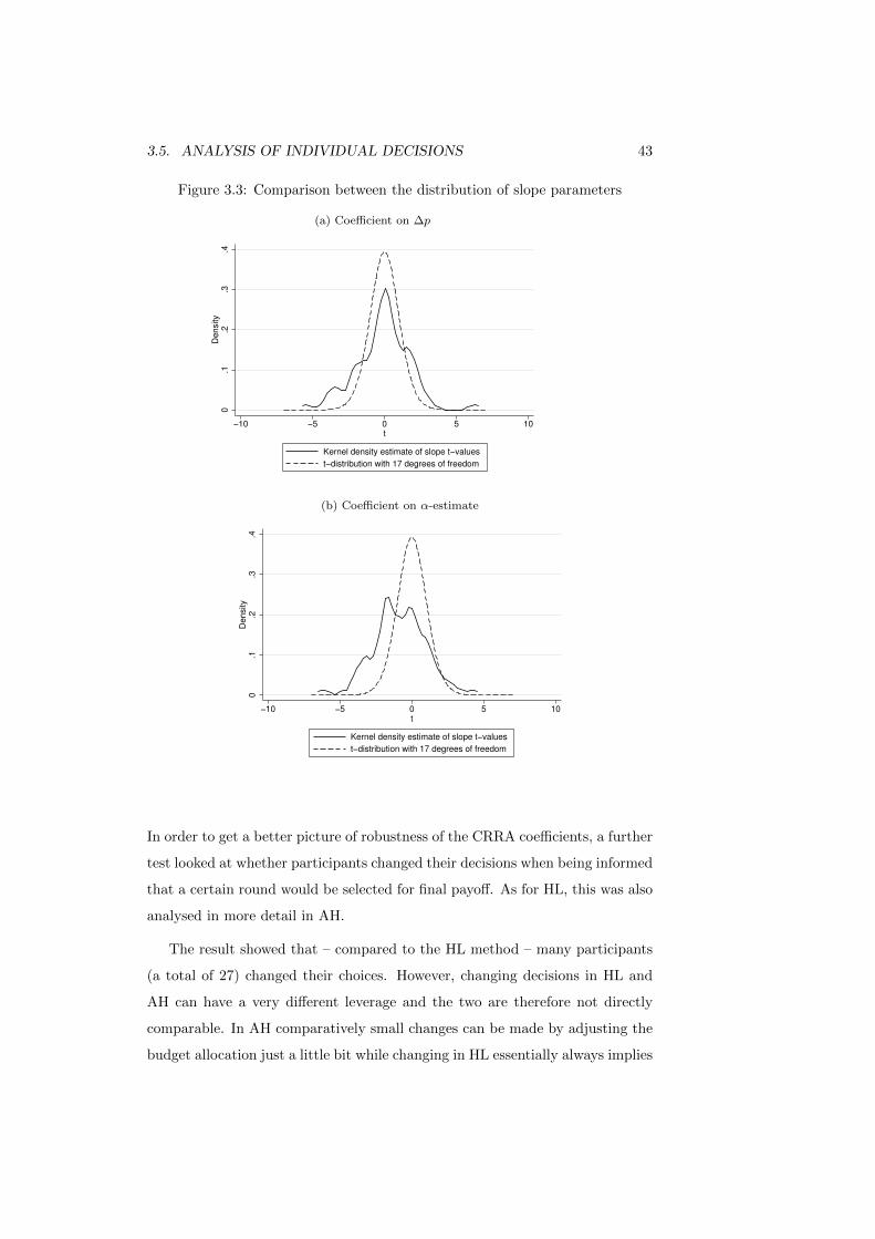
3.5. ANALYSIS OF INDIVIDUAL DECISIONS 43
Figure 3.3: Comparison between the distribution of slope parameters
(a) Coefficient on ∆p0
.1.2
.3.4
De
nsity
−10 −5 0 5 10t
Kernel density estimate of slope t−values
t−distribution with 17 degrees of freedom
(b) Coefficient on α-estimate
0.1
.2.3
.4D
en
sity
−10 −5 0 5 10t
Kernel density estimate of slope t−values
t−distribution with 17 degrees of freedom
In order to get a better picture of robustness of the CRRA coefficients, a further
test looked at whether participants changed their decisions when being informed
that a certain round would be selected for final payoff. As for HL, this was also
analysed in more detail in AH.
The result showed that – compared to the HL method – many participants
(a total of 27) changed their choices. However, changing decisions in HL and
AH can have a very different leverage and the two are therefore not directly
comparable. In AH comparatively small changes can be made by adjusting the
budget allocation just a little bit while changing in HL essentially always implies

44 CHAPTER 3. RISK ATTITUDE CONSISTENCY
a significant shift in measured risk attitudes. However, empirically this was not
a source of large difference, as in AH the percentage change of those individ-
uals that revised their decisions was noticeable. On average, participants that
changed their choices moved 12% towards safer choices and absolute changes
were 30%.
Hence, this result indicates that most participants (65%) made their best-
informed choice before. Those who did change, however, often made large
changes. About 34 of them made changes of 17% or more and numerous changes
are at the rate of 40% or more. Here, but also for the HL method, this raises
the question if revised choices are “better”in their cross-method stability. It
was therefore tested if the revised specifications would have implied a higher
consistency then the aggregate choices, but there did not seem to be further
improvement of consistency with previous choices (i.e., individuals that made
changes did not only do so when they were able to correct an outlier). There-
fore all participants (changers and non-changers) were treated the same by using
their original choices. However, the fact that a lot of switching is observed can
be viewed as a further indication for lack of consistency within the AH method.
Again, as for the HL method potential reasons for changing decisions were
investigated. Some variables were correlated with decision changes in the AH
method. Non-native speakers were more likely to make changes (correlation
of 24%), indicating that understanding the task might play a role.11 Age and
gender, however, did not play a role. Furthermore, individuals with higher
values of α are less likely to change their choices (correlation of 22%). However,
these relationships do not seem to be strong. Individuals who change their HL
choice are not more likely to do so for their AH choice as well, indicating that
switching is not correlated with individual-specific unobservables.
In the last step it was investigated if using average CRRA coefficients derived
in the AH method allowed to reliably classify participants into broad categories
of risk averse, risk neutral and risk loving individuals. Therefore it was tested
whether the average CRRA coefficient α was significantly different from one (or
r 6= 0 using HL’s terminology) using confidence intervals of 2 within-subject
standard deviations. The result from this analysis showed that only for 5 par-
11As the variance of choices does not decrease from the first to the second round in AH, itdoes not seem to be learning over the rounds which drives the effect.

3.5. ANALYSIS OF INDIVIDUAL DECISIONS 45
ticipants out of the 78 the CRRA coefficient α was significantly different from
one; these 5 participants were risk averse and all other participants were approx-
imately risk neutral. Main reason for this is that for almost all participants the
estimated standard deviation on α is larger than 0.3, as can be seen in Figure
3.4.
Figure 3.4: Distribution of standard deviations (on α) of experimental partici-pants in AH
0.5
11.5
Density
0 1 2 3 4Distribution of AH−alpha standard deviations for individuals
3.5.2 Comparison across methods
The data collected in this study also allows to compare the two risk elicitation
methods on a within-individual basis. One way to do so is to try to make
predictions based on one method about how an individual would have made
decisions using the other method. Following this rationale, the average risk
aversion coefficient derived using the AH method was used to predict how an
individual with this parameter would have decided in the HL framework.
Following this procedure would have predicted 76% and 75% of decisions in
the two rounds of the HL method, respectively. However, in this comparison any
individual that has multiple switching points (MSP) will have some incorrect
predictions, even if both methods estimate the same coefficient. To alleviate
this effect, only individuals with SSPs were looked at, which showed 83% and
82% correct predictions for single (rows of binary) HL choices (that is, not the
46 CHAPTER 3. RISK ATTITUDE CONSISTENCY
overall implied risk attitude) over the two periods. These numbers indicate a
high level of comparability.
However, these numbers have to be interpreted with care. The reason for this
is that AH was used to determine individual-specific risk attitudes and based
on these individual values choices in HL were predicted. A simple benchmark
is to assume all participants have the same risk attitude and see how well this
counterfactual can predict choices made in HL. For this, the probably simplest
was to assume all individuals to be risk neutral. This should bias the comparison
to the favour of the AH method as aggregate analysis for both methods indicates
risk aversion. Nevertheless, assuming these risk neutral participants would have
predicted choices made by individuals under the HL method equally well (85%
and 82%, respectively). This implies that individual-specific estimates derived
using AH do not outperform the counterfactual.
Another approach is to simply use the categorisation of participants into
groups with different risk attitudes as in Table 3.2. Using this procedure, indi-
viduals were allocated into these risk categories according to the two methods.
Using this approach, 10% of participants were grouped into the same risk atti-
tude category by both methods. Main reason for this is that the AH method (on
average) classifies individuals as more risk neutral than the HL method. In this
sense one could say the AH method “shifts”behaviour of individuals towards
risk neutrality. In this logic, an average shift of 27% is observable; however,
the shift is not only in one direction (the average absolute shift is about 33%)
and when looking at the ranked correlation on allocations to risk categories the
ranked correlation ρ is only 38%. Figure 3.5 illustrates this relationship.
3.6 Conclusion
Using the risk elicitation methods developed by HL and AH, the experiment
described in this chapter tested their internal and external consistency across
and within individuals. The analysis of results presented in the previous sec-
tion shows that within method correlations of about 60% to 70% of decisions
between periods could be established. Comparatively, cross-method predictions
and correlations were smaller and somewhat consistent estimates can only be

3.6. CONCLUSION 47
Figure 3.5: Allocation of individuals into risk categories by HL and AH
Very risk loving
Risk neutral
Risk averse
Highly risk averse
Highly risk loving
AH
Very ris
k loving
Risk ne
utra
l
Risk av
erse
Highly ris
k av
erse
Stay in b
ed
HL
The number of individuals at a point is indicated by the size of the dot. The line displays
the corresponding linear fit.
established on an aggregate level.
Another central finding of the study was that the two methods did not seem
to be procedurally invariant, both over the full subject pool (as visible in Table
3.2), as well as on an individual level. This seems undesirable considering that a
priori one would have guessed that the two methods would yield similar results
and it seems difficult to determine a better method ex post. The attempt was
to use two methods which were based on the same theoretical framework and
that had the same decision variable. Therefore, this puzzle of cross-method
inconsistency does not seem to be rooted in the goal to measure different things
or the decision variable, as in both methods individuals choose over probabilities.
This difference of a priori comparability and ex post divergence of the methods
can also not be resolved empirically given the data, as none of the additional
variables explained the difference and any reasoning seems highly speculative
given that the two methods have the same theoretical motivation.
Still, one could conjecture that the tasks were not sufficiently explained and
did not point out the logic of the methods (e.g. the use of SSPs in the instruc-
tions), leading to higher inconsistencies or that something in the design led to

48 CHAPTER 3. RISK ATTITUDE CONSISTENCY
an increase in inconsistency. However, the study used relatively standard in-
structions, included test questions and supported participants when they had
questions. Any protocol effects would be unintentional. Additionally, a con-
jecture could be that presenting the full choice list for HL at once in contrast
to presenting choices sequentially in AH might have an influence on decisions.
However, one would prefer a method with desirable characteristics to be robust
to such small changes, particularly as presenting HL choices sequentially would
be likely to further decrease within-individual consistency.
While there are no clear means to determine which of the two methods used
is the correct or superior one, from the results it can at least be evaluated in how
far the desirable characteristics mentioned in the beginning are met by the two
methods. Firstly, in the aggregate both methods allow for making statements
about the overall risk attitudes of the subject pool and one would conclude
that the subject pool is on average (moderately) risk averse. This confirms a
general result of the literature that on average individuals prefer safe options to
gambles. This is a first, though relatively minimal, empirical statement about
the two methods. The conclusion is true for both methods, although results
using the method by AH would suggest that most individuals are more centred
around risk neutrality.
However, while both methods are able to make a statement about the risk
attitude of the overall subject pool, it seems difficult to reliably infer the risk
attitude of an individual from the methods. Given that both methods take their
starting point in an individual-based utility function, it appears undesirable that
an elicitation method is essentially not very good in determining usable and
reasonably stable values in terms of the theory it was designed for. Furthermore,
adding a second measurement from either method for many participants did not
lead to decisions which implied the same coefficient of risk aversion. While this
does not invalidate the results of the methods, it clearly limits the scope of what
they can be used for in terms of individual-based analysis.
While individuals were more consistent over the two rounds in the HL
method than the AH method, for both methods it seems problematic to clearly
identify the risk attitude of an individual. Over the 18 decisions in the AH
method, it was not possible to identify more than 5 of 78 participants having a

3.6. CONCLUSION 49
CRRA coefficient significantly different from α = 1, although the overall picture
suggests that there is risk aversion in the population.
Upon first sight the HL method performs better on this ground, but still
only 22 participants made consistent decisions, and again for most participants
it is unclear whether they are risk averse, risk neutral or risk seeking. Indeed,
in both methods it seems that not only small errors are described as inconsis-
tencies, but results are shifted in a way that is crucial for the interpretation and
meaningfulness of estimated coefficients. This conclusion remains despite the
fact the HL task was only repeated over two rounds and one would conjecture
that increasing the number of repetitions might lead to more inconsistencies.
The analysis of the HL method can be improved by disregarding or simplifying
many inconsistent or mistaken choices that are observable in the data, but this
might not be advisable, as a study by Jacobson and Petrie (2009) has shown.
In any case, HL includes many choices which contribute to the stability of the
method, but are not too interesting in themselves: In HL, almost half of the
choices are only made to determine if individuals are at the extremes of the
scale of risk attitudes, as only being pivotal decisions for individuals with pref-
erences implying high degrees of risk aversion or risk loving. However, most
individuals display rather moderate levels of risk aversion or loving, an exper-
imental observation which is also observed in daily life (probably to an even
larger extend).
Finally, this study also provides information on individual-level consistency
between the two methods, finding ranked correlations of 38% between the meth-
ods. This is surprisingly close to what Isaac and James (2000) found in their
paper comparing risk attitudes of individuals using a first-price auction and the
BDM procedure, which was the first approach comparing two elicitation meth-
ods on an individual level. As most of the literature before, one would read
these individual-based cross-method correlations as (somewhat unsatisfactory)
low.
Furthermore, in this study there were not many superconsistent individuals
as, for example Anderson and Mellor (2009) found in their study. At least
in the subject pool in this study individual inconsistencies were observable for
many participants. The low correlations are also due to the low consistency of

50 CHAPTER 3. RISK ATTITUDE CONSISTENCY
decisions for even the same procedure, which can be observed in the within-
method benchmark. In this sense, ρ=38% is not so terrible, though evidently
one would like to have risk elicitation methods with more consistency. This is
particularly crucial from the perspective of a practitioner for whom measuring
risk attitudes is not the last step and ultimate goal, but who would like to use
this information for further analysis, for example when quantifying the role of
risk attitudes in decisions where risk and other elements determine experimental
outcomes jointly. The effect would also not be mediated if the reliability of
measures can be improved through further repeated measurements (Wilcox,
2008, shows that many repetitions are required for reliable risk attitude measures
in HO and a similar conclusion is likely to be true for other methods), as the
time that can be designated to risk elicitation in applied studies is often limited
and letting participants make hundreds of choices before the core experiment
starts is not feasible
To conclude, it seems that both risk elicitation methods, despite providing
some usable aggregate results are not as good as it would be desirable in deter-
mining individual risk attitudes, which remain ambiguous for most participants.
Given the desirable criteria of any method as described in the beginning of the
chapter, both methods seem not to meet more than the most basic ones, primar-
ily allowing to make statements about the general prevalence of risk attitudes
in the subject pool. Unfortunately, this effect is even more severe when adding
another risk elicitation method, which shows that estimates are not method
invariant. In the study presented here this was true both from a participant-
aggregate point of view as well as on an individual level. This is disappointing
considering that risk aversion, based on the notion of individual utility, is es-
sentially an individual-based concept.

Chapter 4
Sources of experimental
risk attitudes1
4.1 Introduction
As already pointed out in the previous chapter and the introduction, the com-
monly used concept of risk aversion in economics is mainly motivated in a the-
oretical framework, although much of its intuition is also based on the daily
observation that people avoid or are at least hesitant to take risks. Both the
theoretical as well as common sense understanding of risk aversion is based on
the idea that an underlying element reflects that some individuals make more
risky choices than others.2 Besides providing interesting theoretical and exper-
imental insights, risk attitudes also have clear implications for decision making,
be it for choices in daily life, business or policy. Hence, understanding decision
making under risk is of central importance for individuals, companies and pol-
icy makers. However, it seems non-trivial to clearly measure risk attitudes of
individuals in an experimental laboratory environment, which makes it difficult
to use experimental findings for informing decision makers.
In contrast to economists’ intuition, a large number of studies documents
1This chapter builds on joint work with Markus Schaffner.2The term risk aversion was originally coined with an expected utility (EUT) paradigm
in mind, where the curvature of the utility function can be understood as a measure of riskaversion. The main lines of argument in this chapter are in the EUT world, but one excursionand extension into a non-EUT framework is included.
51
52 CHAPTER 4. RISK ATTITUDE SOURCES
that individual-level inconsistencies in experimentally measured risk attitudes
are quite common (e.g. Isaac and James, 2000; Berg et al., 2005; Hey et al., 2009;
Dave et al., 2010). Individual measures obtained from different methods used
to infer risk attitudes provide conflicting results and can even differ within one
method over time (Harrison et al., 2005a). Also results from the previous chapter
support this evidence. However, the drivers of instabilities or inconsistencies are
often unclear.
Starting from these observations, this chapter presents a study that tries
to link theory-motivated risk aversion measures, demographics (age and gen-
der) and personality traits, the physiological state of individuals and a stressful
trade-off decision when presented with a dilemma. As in the preceding chapter,
elicitation methods by HL and AH are used to gather information about subject
pool and individual risk attitudes. Personality traits are elicited using a ques-
tionnaire. In the dilemma situation participants have to decide to save one of
two swimmers from drowning after watching a video describing this situation.3
To get physiological information of experimental participants, throughout
the experiment the electrocardiogram (ECG) of participants was monitored
during the decision making process. The chapter uses heart rate variability
(HRV) as a physiological measure, which has been linked to the processing of
information in the brain (Critchley et al., 2003). As outlined in the introduc-
tion of this thesis, using HRV is an interesting research frontier when trying
to understand economic decision making, because it carries an interpretation
reflecting the sympathovagal balance of the decision maker during the decision.
Confirming results from the preceding chapter, the study included in this
chapter finds that results from the two risk elicitation methods are correlated,
but that one method serves as a shifter of results towards more risk neutrality.
This difference is partly due to a difference of the gender effect. Personality
3The discussion of dilemmas has a long tradition in philosophy, particularly in thoughtexperiments. The dilemma used here is similar to the doctor’s dilemma or a more benignversion of Sophie’s Choice as described in Greenspan (1983) who discusses, like Marcus (1980),emotions and the feeling of guilt when deciding in a dilemma. Emotional engagement is alsoemphasised in a more recent experimental study which investigates neural correlates thatare connected to moral judgements in dilemma decisions (Greene et al., 2001), finding thatemotions play an important role in the decision making process. This second study canalso be seen as a first study in decision neuroscience (Shiv et al., 2005), which similar toneuroeconomics investigates neural correlates of behavioural decision making, a field to whichthis study connects to as well.
4.2. BACKGROUND AND HYPOTHESES 53
traits account only for a small fraction of the difference, if anything. With
respect to HRV measures, the study establishes a link between risk taking and
the physiological state for at least one of the methods, indicating that more
stressed individuals are more risk averse in the experiment. Finally, there is
some evidence that personality traits have an influence on whether individuals
made a decision in the dilemma situation or if they hesitated too long, failing
to make any decision. However, there was no connection between the dilemma
decision and risk attitudes, and, surprisingly, the HRV did not serve as an
indicator for the ability to make a decision.
4.2 Background and Hypotheses
The use of most elicitation methods to measure risk attitudes of individuals
builds on the idea that these are stable individual-specific characteristics and
traits. But what are determinants of risk attitudes and can they potentially
explain some of the differences in the results between different risk elicitation
methods? For example, gender and age effects, which have been found to vary
with risk attitudes, might be more or less pronounced between methods. For
example Hartog et al. (2002) study survey data of groups in the Dutch popu-
lation and connect risk attitudes with individual demographics. They find that
in general terms gender and age are related to risk attitudes. Similar results
are also included in Halek and Eisenhauer (2001). The experimental economics
literature also suggests that, if anything, females display more risk aversion, al-
though this results is not always significant (see Eckel and Grossman, 2008, for
an overview). Another example is included in Harrison and Rutstrom (2008).
Furthermore, different methods, although economists usually think about
risk aversion as a one-dimensional or baseline trait, could reflect risk attitudes
of risk domains. For example, one method might elicit primarily financial risk
taking, another method risk taking in a health and safety context. The notion
of domain-specific risk taking is common in psychological research (Weber et al.,
2002), while economists usually think of a more general (underlying) risk atti-
tude. However, general risk taking is nevertheless related to domain-specific risk
taking (see, for example Dohmen et al., 2011). Personality traits could influence

54 CHAPTER 4. RISK ATTITUDE SOURCES
how much risk aversion an individual displays in different domains (Soane and
Chmiel, 2005) and shift results in certain directions between methods.
It is therefore interesting to link the two laboratory-based risk elicitation
methods and personality traits, which are measured based on the so-called Big
Five personality classification system introduced by Goldberg (1981).4 Based
on results by Nicholson et al. (2005), who study the connection between per-
sonality traits and risk in specific domains as well as general risk attitudes, the
expectation is that experimentally elicited risk taking will be positively related
to extroversion and openness and negatively related to neuroticism, agreeable-
ness and conscientiousness.
Based on the study in the previous chapter, the results from the two risk
elicitation methods are expected to be different, but correlated. The hypothesis
made in the design of this study was that personality traits are one source for
explaining differences. This hypothesis is based on previous findings indicating
that risk attitudes across different domains are differentially related to personal-
ity traits and the different presentation of the two methods could frame attitudes
into different risk taking domains. Another hypothesised source was the role of
gender in the two methods, due to the mixed evidence of its influence in prior
literature. The hypothesis with respect to the ability to decide in the dilemma is
that it depends on personality traits as well as on risk attitudes: Both are inter-
preted as fundamental individual-specific characteristics and as such potentially
connected to how hesitant individuals are in their decision making.
Throughout the experiment the physiological state of participants was mea-
sured, reflected in their HRV. HRV is used as objective data that indicates
emotional and mental processes that are taking place within the individual and
that are connected to the decision making process. The hypothesis is not that
these measures are related to the decisions taken in the experiment in a way
that they are able to explain behaviour. Rather, they are correlates reflecting
mental states. Using reverse inference as described in the introduction, the fact
that decisions and changes in the physiological state occur at the same time is
interpreted such that they are causally related.5 Using this approach, it is anal-
4Also see John et al. (2008) for developments in research using the Big Five.5As outlined in the introduction there is also some reason to believe in a potentially causal
link between HRV and mental states.

4.3. EXPERIMENTAL DETAILS 55
ysed if risk taking in the experiment as well as the propensity to decide in the
dilemma situation are connected to the physiological state of individuals. Both
are conjectured to connect to HRV through emotions: Risk has been argued
to have a feelings-component (Loewenstein et al., 2001), and so has decision-
making in dilemmas (Greene et al., 2001). HRV, conversely has been shown to
reflect emotions in several studies (Appelhans and Luecken, 2006; Lane et al.,
2009; Wallentin et al., 2011) and can be interpreted as a correlate of emotions
in experiments.
The a priori conjecture is that greater risk taking is related to higher ex-
citement, emotional engagement, or stress.6 While this is hypothesised for both
methods, again the framing of the risk elicitation tasks into potentially differ-
ent domains could lead to a differentially strong effect of HRV across methods.
However, if individuals are able to make their excitement-optimal choice in the
experiment, a weak ad hoc relationship between the riskiness of a choice and
HRV measures are also reasonable. In this case, it might, however, still be possi-
ble to observe differences across individuals in risk taking, which would indicate
if generally more or less excited individuals take higher risks.
With respect to the willingness to make decisions in the dilemma, the ex-
pectation is that physiologically more excited individuals, once controlling for
personality traits, are more likely to make the decision of saving one of the
swimmers, as it helps them to overcome the tendency to hesitate. Similarly,
more risk averse individuals would be expected to be more hesitant in their
decision making and hence be less able to decide in the dilemma. However, it is
not hypothesised that this effect is different across methods, but should connect
to a common underlying risk attitude factor.
4.3 Experimental details
The experiment was run in a computer laboratory over several sessions on two
days in February and July 2011 with a total of 75 participants. Participants were
recruited from an online pool of about 2000 students using ORSEE (Greiner,
6This assumes that facing risky choices, hence the experiment itself, does not have a majorimpact on the physiological state of the participants, but that HRV changes mainly mirrorthe process of decision-making.

56 CHAPTER 4. RISK ATTITUDE SOURCES
2004). Participants were on average 21.8 (s.d. .5) years old, in about equal
shares of gender (51% were male) and were mostly enrolled in various business
degrees, such as accounting or marketing, as well as economics.
The invitation to the experiment included information about the length of
the experiment and information that the heart rate of participants would be
measured during the experiment. Upon arrival at the lab, participants were
welcomed and asked to put on the heart rate monitor. Afterwards, they were led
to a computer and asked to go through the experiment at their own pace. Most
participants needed about 30 minutes to do so. When participants had finished
the experiment, they were asked to raise their hand, were given an envelope with
their payment and returned the heart rate monitor. Participants were paid a
show-up fee of five Australian dollars for participating in the experiment plus
a second amount according to their decisions in the risk elicitation task. Using
this procedure, participants earned, on average, about 30 Australian dollars for
their participation. The computer-based experiment, which used experimental
software CORAL (Schaffner, 2012), continued through five major stages.
In the first stage participants were asked personality-related questions of
the Big Five Inventory (BFI, John et al., 1991) and some other personality-
related questions. The second stage of the experiment consisted of a relaxation
phase during which participants were shown a picture of the ocean and heard
background sound of the sea rushing on headphones. Participants were asked
to close their eyes, take a sea shell from the table into one of their hands,7 to
listen and relax. The relaxation phase lasted for five minutes. The purpose of
the relaxation phase was to get participants down to an undisturbed baseline
heart rate.
The third stage of the experiment consisted of two rounds in each of which
first the risk elicitation method by HL was played, followed by the method by
AH. For HL, the set-up with slightly lower stakes was played in the first round,
followed by the first round of AH, then HL with the slightly higher stakes,
followed by the second round of AH. The order of the two methods was not
switched because previous results did not hint to any order effects as described
in the preceding chapter.
7The purpose of the sea shell was to prevent participants from crossing their arms anddistorting the heart rate measurement by interfering with the electrodes on their chest.

4.3. EXPERIMENTAL DETAILS 57
After having finished the risk elicitation tasks, participants advanced to the
fourth stage and were shown a short video of about one minute length. The
video showed a life saver walking to the beach and then two people drowning in
the water. The video was supplemented by a voice that asked the participant
to imagine being in the role of the life saver and having to make a decision of
saving one of the two drowning people. Furthermore, information was included
saying that only one of the two could be saved (due to the urgency of the
situation: “you will only be able to save one of them”). After the end of the
video, participants automatically advanced to a decision screen that asked them
to save either the person on the left or on the right from the video they had
just seen. Snapshots of the video showing a hand coming out of the water were
included with the two choice options of either saving the person on the left or on
the right. Furthermore, a button for “more information”was included. Clicking
on this option led to a screen describing more hypothetical options one could
contemplate about, but that would require time after which both swimmers
would have drowned.8 An option to see even more information (which then,
however, said that there was no more information) and the option to return to
the decision screen were also included on this screen.9
Participants were given 20 seconds after entering the decision screen to make
a choice and save one of the two swimmers. However, participants were not
informed about this time limit and did not see any clock ticking down. The
reason for this was to identify those individuals who would be able to understand
the urgency of the situation and make a decision. In case they succeeded to do
so, they were shown a short video in which the swimmer they had chosen to
save was rescued. In case they did not make a decision and exceeded the time
limit, a time-out screen appeared informing them that they had failed to make
a decision.
Finally, participants advanced to a short demographic questionnaire that
included information about gender, age, student status and some health related
measures, marking the end of the experiment.10
8These options included the possibility to walk back to the life save station and call formore help, look around for other helpers, organise more equipment, etc.
9Beyond this, this screen only served the purpose of using up participant’s time. Manyparticipants clicked one or even both “more information”buttons, and some of these stillmanaged to save one of the two swimmers.
10This was done to detect potential problems that could distort heart rate measures, for

58 CHAPTER 4. RISK ATTITUDE SOURCES
4.4 Experimental results
4.4.1 Analysis separated by methods
For both elicitation methods used in this study, individual risk attitudes and
individual-specific risk aversion coefficients αi (assuming Ui(x) = xαi) in an
expected-utility (EUT) framework can be estimated. For AH, it is even possi-
ble to determine a coefficient of risk aversion for every choice made (αit), given
this utility function. Estimating these individual-specific values for both meth-
ods allows to get an idea about the distribution of individual risk attitudes for
both methods and to make some general comparisons between them. Figures
4.1 (a) and (b) illustrate the estimated values (separated by gender) for those
participants with s.d.(αit) ≤ 3 for AH and participants with less than 4 switch-
ing points in HL. In AH this leads to the exclusion of 5 individuals and in HL of
6 individuals. These restrictions were used as αi-estimates for these individuals
do not appear very meaningful in the context of EUT and of a utility function
as described above. Including those individuals does not qualitatively change
the overall distribution, but makes the graphs less readable.
As can be seen in these overviews, there seem to be differences between the
distributions of individual estimates by gender. Women seem to be more risk
loving than men in the AH method, but more risk averse in the HL method,
which is in line with previous findings. The estimated individual values for the
methods, αAHi and αHLi , are significantly correlated at the levels of .53 for males
(p=.002; Spearman’s ρ=.40, p=.025), .41 for females (p=.027; ρ=.50, p=.005),
and .42 for both males and females (p=.001; ρ=.38, p=.002).
In order to investigate the first hypothesis that for both methods a relation-
ship between gender, age and risk attitudes could be established, these were
included in the method-specific estimation procedure. Similarly, conjecturing
that there would be a relationship between some of the personality measures,
HRV measurements and risk attitudes, in a next step these variables were added
to the estimation. In both methods a potential relationship between the vari-
ables was tested using maximum likelihood estimations.11 Table 4.1 reports the
example medications or smoking. There were, however, no indications for specific healthmeasures that affected the recording of any participant.
11See Harrison and Rutstrom (2008) for a guideline on estimation proce-

4.4. EXPERIMENTAL RESULTS 59
Figure 4.1: Distributions of αi-parameters estimated using the two methodsseparated by gender
(a) AH
0.2
.4.6
−1 0 1 2 3x
Estimate AH for males Estimate AH for females
(b) HL
0.5
11.5
2
0 .5 1 1.5 2
x
Estimate HL for males Estimate HL for females
results of this procedure.
dures. Here, in the estimation the Likelihood functions used were LHL =∏18i=1
[Pr(yi|Xi, α, β)yi · (1− Pr(yi|Xi, α, β))1−yi
]with yi = 0 if option A was cho-
sen, yi = 1 if option B was chosen and assuming Pr(yi = 1|Xi, α, β) reflected in a
normal distribution for HL and LAH =∏18i=1
[probk|Xαi∑maxprob
j=1 probj |Xαi
]with probk indicating
the probability chosen by the decision maker and probj ∈ [1, . . . ,maxprob] indicating allprobabilities not chosen for AH. For joint estimations in the analysis described further belowLjoint = (LHL)d · (LAH)1−d with d = 1 for HL observations and d = 0 for AH observationswas used.

60 CHAPTER 4. RISK ATTITUDE SOURCES
Table 4.1: Determinants of α-estimates
AH1 AH2 AH3 HL1 HL2 HL3
αconstant 0.96* -0.19 1.14** 0.65*** 0.01 0.74***
(0.55) (1.20) (0.57) (0.11) (0.40) (0.11)Female 0.10 -0.16 -0.13 -0.16*** -0.13** -0.19***
(0.20) (0.21) (0.20) (0.05) (0.06) (0.06)Age -0.01 -0.00 0.00 0.00 0.01* 0.00
(0.03) (0.03) (0.03) (0.00) (0.00) (0.00)Extraversion -0.00 0.07*
(0.14) (0.04)Agreeableness 0.03 0.08*
(0.20) (0.05)Conscientiousness 0.10 0.02
(0.17) (0.05)Neuroticism 0.11 0.01
(0.20) (0.04)Openness 0.36 0.06
(0.32) (0.07)HRV ( LF
HF) -0.21* -0.21* -0.02 -0.04
(0.12) (0.12) (0.04) (0.04)
N 1188 1044 1080 1152 1026 1080
The table illustrates the influence of potential determinants for each elicitation method of AHand HL. *** indicates significance at the 1% level, ** 5% significance and * 10 % significance.Standard errors (in brackets) are clustered by individuals. The availability of HRV data hasreduced the sample between estimations (due to missing or unreadable data). The HRVmeasure for equations AH1−3 represents the average HRV during the AH stage and forequations HL1−3 the average HRV during the HL stage.
The results from the estimation support the first impression that the role of
gender is different between the two methods. I.e., there is no apparent relation-
ship between gender and risk-taking in AH and a significant negative relation-
ship in HL. Similarly, there is no age effect in the AH method and a statistically
small effect in the HL method.
Adding personality characteristics and HRV measures does not change the
significance level of any of the variables in the AH method. For AH none of
the personality characteristics has a significant influence on decisions. However,
there is a significant relationship between the αAH estimate and the HRV ( LFHF ).
A negative coefficient on the HRV variable indicates that individuals who were
physiologically less stressed during this task of the experiment took more risk;
or vice versa, more stressed individuals displayed more risk aversion.
In the HL method, further adding information on personality traits shows
that some of the personality characteristics have a significant influence on the

4.4. EXPERIMENTAL RESULTS 61
level of risk aversion. There is a positive effect of extroversion and agreeableness.
For extroversion, this is as expected. For agreeableness, the result is in the
opposite of what was expected based on previous findings. However, as the size
of the effect is relatively small, maybe not too much should be read into this
result. There is no clear evidence that for the HL method HRV is significantly
related to risk-taking.
While the physiological measure of the HRV is insignificant for the HL
method, the relationship is significant for the AH method. However, gener-
ally both have the same direction.12 This difference could partly be due to the
fact that the level of risk taking in HL is relatively stable between the choices,
while the risk taken between AH choices can vary greatly. For a slightly risk
averse individual the first 3 and the last 3 rows of the choice list of HL might be
straightforward, while only the pivotal ones are critical. For AH, on the other
hand, each period a full range of risky and riskless options can be chosen. In
fact, most individuals make both risk-seeking and risk-averse choices in the AH
method during the course of the experiment. Hence, individuals vary more in
their level of risk-taking and deviations from optimal stress-risk points can be
detected in the data.13
Another possible explanation is that the two methods measure different types
of risk taking (which could also be reflected in the difference of their estimated
values). The difference in the significance level between the methods could then
be explained by the conjecture that one of the methods, AH, is simply more
strongly related to the physiological state then the other.
Excursus: Results considering a non-EUT framework
All of the analysis so far has focussed on an EUT framework. This section
goes beyond EUT and includes a small excursion assuming that the patterns of
experimental choices do not only represent utility curvature, but also probability
weighting. However, as was mentioned before, both HL and AH were designed
to elicit risk attitudes under EUT. As a result, given the data generated in the
12The sign of this relationship was visible throughout basically all alternative specificationslooked at.
13Indeed, there is some evidence that in the AH method in periods where individuals havea lower LF
HF, they take more risky choices. However, this effect is not significant.
62 CHAPTER 4. RISK ATTITUDE SOURCES
AH method, the estimation of parameters of a probability weighting function is
not possible, as the decision maker chooses over a wide range of probabilities.
In fact, choices in AH are only interpretable in a meaningful way when EUT is
assumed.
Also the HL method mainly makes sense when an EUT framework is as-
sumed as under EUT switching points from the less to the more risky option
contain straightforward information. However, in the presence of probability
weighting these interpretations are not as clear any more, as multiple switching
points can become reasonable. As a consequence, it is not easy to determine if
multiple switching points result from small errors in decisions made, or if they
are due to probability weighting. Nevertheless, technically, it is possible to find
estimates for a given probability weighting function with data generated using
the HL method, although estimation results are usually statistically insignifi-
cant, particularly on an individual-specific level. In the following the estimation
results assuming probability weighting under the HL method are included. Due
to the structure of the AH data, this analysis cannot be extended to any of the
analysis that involves AH or both risk elicitation methods.
Distributions of values estimated for α and γ
In the following estimation procedures a probability weighting function of the
functional form wi(p) = pγi
(pγi+(1−p)γi )1/γi was assumed. The utility function for
risky choices can be written as
Ui(Xi) = wi(p) · Vi(Xi) (4.1)
with Vi(Xi) = Xαii as before. Individuals are assumed to choose the option with
the highest expected value under probability weighted outcomes, where wi(p)
assigns objective probabilities a subjective individual weight. For choices made
in the HL method, this allowed to estimate an average αi=.86 (s.d. =.33) and
a γi=1.10 (s.d. =.11). Hence, there is some evidence for probability weighting,
however, a γi which is significantly different from 1 (representing no probability
weighting) cannot be determined for most participants; this can be explained
by the relatively small number of choices each individual makes. Figures 4.2

4.4. EXPERIMENTAL RESULTS 63
(a) and (b) illustrate the distributions of the estimates. For this overview and
in the following analysis the sample was restricted to 45 individuals that had a
single switching point (SSP) in both periods of HL in order to make the graphs
readable and to ensure convergence of the maximum likelihood models.
Figure 4.2: Distributions of αi- and γi-parameters estimated using HL
(a) Distribution of α
0.5
11.5
Density
.5 1 1.5 2
Estimates for individual alphas
Kernel density estimate
(b) Distribution of γ
12
34
Density
.9 1 1.1 1.2 1.3 1.4
Estimates of individual gammas
Kernel density estimate

64 CHAPTER 4. RISK ATTITUDE SOURCES
Potential determinants of α and γ
In an extension of the analysis investigating factors that drive risk attitudes
under EUT, it was also investigated if demographics, personality traits and
physiological states were related to α and γ in a joint estimation. Table 4.2
shows the results from the main specifications of this analysis. The additional
result emerging from this analysis is observable for the coefficient on the HRV
measure, as there is no clearly significant effect of any of the other variables.
HRV is potentially positively related to utility curvature, which would be con-
trary to the result found for AH and the tendency in HL when assuming EUT.
Here, there is a negative relationship between HRV and probability weighting
observable which indicates that more stressed individuals are more likely to
display inverse S shape-type probability weighting. Taken together these two
effects could indicate that the relationship observable before EUT-based analy-
sis could be driven by probability weighting which cannot be estimated in AH,
but which might nevertheless play a role in decisions over AH choice options.
4.4.2 Analysis of the two methods with jointly estimated
values for α
Both methods by HL and AH allow to think of the same kind of risk parameter
α as they were designed with a utility function of Vi(Xi) = Xαii in mind.
Consequently, the following analysis proceeds with estimating an individual’s
risk attitude using a joint estimation procedure with data from both methods.
Figure 4.3 illustrates the distributions of these estimates separated by gender.14
As visible before, estimates for women were more dispersed. However, it is not
evident whether they are more risk loving then men from results of the joint
procedure.
Assuming this joint structure, it was investigated whether any variables had
a significant influence on the jointly estimated risk attitude. Table 4.3 illustrates
different specifications. Rather surprisingly, no variable seems to have a signif-
icant impact on α. While this could indicate that these variables simply have
no significant connection to the risk attitudes, another reason could be that the
14The same individuals were excluded for the joint estimation as described in the method-specific procedures.

4.4. EXPERIMENTAL RESULTS 65
Table 4.2: Determinants of α and γ
REDU1 REDU2 REDU3 REDU4α
Age -0.00 0.00 0.00(0.00) (0.00) (0.00)
Female -0.05 -0.02 0.02(0.04) (0.05) (0.05)
Extraversion 0.09 0.11**(0.08) (0.05)
Agreeableness 0.03 0.04(0.04) (0.05)
Conscientiousness -0.03 -0.01(0.07) (0.05)
Neuroticism 0.00 0.01(0.03) (0.02)
Openness -0.03 -0.03(0.06) (0.05)
HRV ( LFHF
) 0.04 0.06*(0.02) (0.03)
constant 0.73*** 0.50** 0.64*** 0.22(0.06) (0.21) (0.05) (0.26)
γ
Age -0.00 0.01 0.01(0.00) (0.01) (0.01)
Female -0.02 -0.10 -0.28**(0.03) (0.16) (0.13)
Extraversion -0.12 -0.16(0.29) (0.13)
Agreeableness 0.10 0.09(0.10) (0.09)
Conscientiousness 0.07 -0.01(0.24) (0.07)
Neuroticism -0.04 -0.03(0.10) (0.05)
Openness -0.11 0.00(0.11) (0.11)
HRV ( LFHF
) -0.09*** -0.16***(0.02) (0.05)
constant 1.06*** 1.21** 1.22*** 1.68***(0.03) (0.52) (0.05) (0.36)
N 810 774 756 720
*** indicates significance at the 1% level, ** 5% significance and * 10 %significance. Standard errors (in brackets) are clustered by individuals. Theavailability of HRV data has reduced the sample between estimations (due tomissing or unreadable data). The sample is limited to individuals with singleswitching points.

66 CHAPTER 4. RISK ATTITUDE SOURCES
Figure 4.3: Distribution of estimated individual risk attitudes (α) jointly esti-mated:
0.2
.4.6
.8
0 .5 1 1.5 2 2.5
x
Joint estimate for males Joint estimate for females
two methods are measuring (slightly) different things and the joint estimation
averages out some of the effects visible in Table 4.1. Therefore the next section
describes an estimation procedure that allows for the possibility that the two
methods measure different α-values.
4.4.3 Analysis of potential differences between HL and
AH measures
As prior overviews as well as simple correlations indicated that generally the
two methods do not provide the same estimate for αi, differences between the
two methods and potential determinants of such differences were further in-
vestigated. For this, Vi(Xi) = Xαi+∆HLi was assumed with ∆HL representing
the difference between the methods (AH was used as the baseline and ∆HL
hence reflects the additional effect of HL). The results from this estimation are
included in Table 4.4.
As can be seen in Table 4.4, a difference between the methods cannot clearly
be determined. Furthermore, there are no factors that seem to drive differences
– only extraversion seems to play a weakly significant role for having a higher
risk attitude in HL compared to AH. Hence, it cannot clearly be said that a
significant difference between the methods is observable.

4.4. EXPERIMENTAL RESULTS 67
Table 4.3: Determinants of the joint estimation assuming no structural differ-ence between the methods
JOI11 JOI12 JOI13 JOI14 JOI15α
0.72*** 1.00*** 0.12 -0.12 1.14***(0.07) (0.26) (0.85) (0.89) (0.32)
Female -0.00 -0.16 -0.14(0.15) (0.14) (0.13)
Age -0.01 -0.00 -0.00(0.01) (0.02) (0.01)
Extraversion 0.08 0.08(0.12) (0.11)
Agreeableness 0.04 0.08(0.16) (0.12)
Conscientiousness 0.09 0.09(0.13) (0.13)
Neuroticism 0.03 0.03(0.10) (0.10)
Openness 0.19 0.15(0.23) (0.21)
HRV ( LFHF
) -0.15 -0.12 -0.15(0.10) (0.09) (0.10)
N 2160 2160 1944 1944 2016
*** indicates significance at the 1% level, ** 5% significance and * 10 %significance. Standard errors (in brackets) are clustered by individuals. Theavailability of HRV data has reduced the sample between estimations (due tomissing or unreadable data).
4.4.4 Determinants of making a timely decision
Finally, the life saving dilemma was used to investigate if demographic char-
acteristics as well as risk attitudes, personality traits and physiological states
during the decision process were related to the ability of individuals to make
a decision and to save a swimmer (or failing to do so and exceeding the time
limit otherwise). Table 4.5 shows the results of Probit regressions of making a
decision.
As can be seen in Table 4.5, the demographic characteristics of gender and
age had no significant effect on the ability to make a decision. Furthermore,
at least when using the joint estimate of an individual’s risk attitude αi, risk
attitudes did not predict decisions. This is somewhat surprising, as one would
generally assume a more risk averse decision maker to be more hesitant as well;
but this does not seem to be the case.
In contrast, some of the personality traits did have an influence on the de-
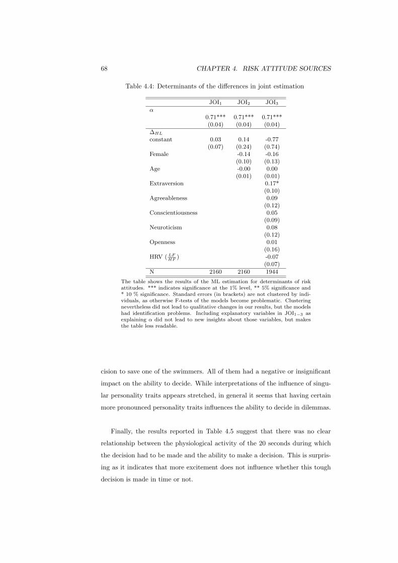
68 CHAPTER 4. RISK ATTITUDE SOURCES
Table 4.4: Determinants of the differences in joint estimation
JOI1 JOI2 JOI3α
0.71*** 0.71*** 0.71***(0.04) (0.04) (0.04)
∆HL
constant 0.03 0.14 -0.77(0.07) (0.24) (0.74)
Female -0.14 -0.16(0.10) (0.13)
Age -0.00 0.00(0.01) (0.01)
Extraversion 0.17*(0.10)
Agreeableness 0.09(0.12)
Conscientiousness 0.05(0.09)
Neuroticism 0.08(0.12)
Openness 0.01(0.16)
HRV ( LFHF
) -0.07(0.07)
N 2160 2160 1944
The table shows the results of the ML estimation for determinants of riskattitudes. *** indicates significance at the 1% level, ** 5% significance and* 10 % significance. Standard errors (in brackets) are not clustered by indi-viduals, as otherwise F-tests of the models become problematic. Clusteringnevertheless did not lead to qualitative changes in our results, but the modelshad identification problems. Including explanatory variables in JOI1−3 asexplaining α did not lead to new insights about those variables, but makesthe table less readable.
cision to save one of the swimmers. All of them had a negative or insignificant
impact on the ability to decide. While interpretations of the influence of singu-
lar personality traits appears stretched, in general it seems that having certain
more pronounced personality traits influences the ability to decide in dilemmas.
Finally, the results reported in Table 4.5 suggest that there was no clear
relationship between the physiological activity of the 20 seconds during which
the decision had to be made and the ability to make a decision. This is surpris-
ing as it indicates that more excitement does not influence whether this tough
decision is made in time or not.

4.5. CONCLUSION 69
Table 4.5: Probit regressions of decision to save swimmer
SLS2 SLS3 SLS4 SLS5
Female -0.05 -0.15 0.23 0.13(0.30) (0.38) (0.36) (0.44)
Age -0.00 0.01 0.00 0.01(0.03) (0.03) (0.03) (0.04)
αi(JOI11) -0.20 -0.17 -0.12(0.30) (0.28) (0.34)
Extraversion -0.45 -0.98**(0.30) (0.38)
Agreeableness -0.35 0.21(0.36) (0.44)
Conscientiousness -0.57* -0.88**(0.33) (0.41)
Neuroticism -0.61* -0.79**(0.34) (0.38)
Openness 0.10 0.67(0.53) (0.67)
HRV ( LFHF
) 0.00 0.04(0.13) (0.14)
constant -0.27 4.41* -0.47 4.11(0.59) (2.44) (0.65) (2.84)
N 71 61 59 56
The table shows the results of Probit regressions on whether a participantmade a decision to save a swimmer or not. *** indicates significance at the1% level, ** 5% significance and * 10 % significance.
4.5 Conclusion
In the analysis of this chapter, the main goal was to understand if risk attitudes,
measured using two different elicitation methods, demographics and personality
traits are related. Furthermore, it was investigated, how these were connected
to two other types of information, i.e. physiological data and the ability to make
a decision in a dilemma. For this goal information on each of these elements
was collected in an experimental laboratory environment.
The analysis of the experimental data shows that the results from the two
risk elicitation methods are correlated, but do not provide the same results: Cor-
relations as well as ranked correlations are far from one and there also seems
to be a shifter effect between the methods. In AH the distribution of risk atti-
tudes is also wider as it is in HL. With respect to demographics, the distribution
of risk attitudes is more dispersed for females than for males. Women appear
to be more risk taking in AH, though the effect is not statistically significant.
In contrast, they are significantly more risk averse in HL. However, there is no
70 CHAPTER 4. RISK ATTITUDE SOURCES
clear statistically significant gender effect driving the difference between the two
methods when analysing the results of a joint estimation.
In a further step, individual risk attitudes were linked to personality traits
(based on the Big Five). The conjecture was that the different methods could
be linked to different risk domains, and that this fact could be captured by a
different connection to personality traits. However, there was no strong support
for this hypothesis and only some weak evidence showing that more extroversion
and agreeableness are related to more risk seeking HL, while there is no signifi-
cant effect in the AH method. Similarly, looking at the factors driving differences
between the two methods, extroversion seems to play a weakly significant role.
Generally the connection between personality traits and risk attitudes is weak
and mostly insignificant. However, it reduces the gender effect in HL, reflecting
different distributions of personality traits across gender.
Apart from searching for sources of the differences between the elicitation
methods, a main aim was to investigate how risk attitudes and physiological
states were connected. For this, physiological HRV data was collected, using
the LFHF ratio as an indicator which reflects the mental stress during the decision
making process. The analysis tested whether such a relationship exists by in-
cluding the HRV measure of the time during which an experimental participant
made decisions in the risk elicitation task in the estimation procedure for risk
attitudes. Results of this analysis show that the HRV and risk taking are related
in a way indicating that individuals who are less stressed take higher risks in the
AH method.15 The connection between the HRV and risk taking is significant
for AH, but not for HL, although the direction of the effect is the same.16
What does this mean? While one could conjecture that risk taking is some-
thing ad hoc exciting, and expect a positive relationship between α and HRV,
results of this study indicate the reverse. This can potentially be interpreted
as resulting from the fact that risk attitudes are something more basic (and
not determined ad hoc). Less stressed individuals are less averse towards mak-
15Also the quantitative effect appears noticeable. However, due to the estimation procedureused no easily interpretable statement about the marginal effect can be made.
16When allowing for probability weighting the effect reversed for utility curvature and wassignificant for the weighting itself, indicating that more stressed individuals display moreinverse S shape-type probability weighting. This could be interpreted such that the effect onoverall risk aversion might be driven by probability weighting, which could not be estimatedfor AH.
4.5. CONCLUSION 71
ing more risky decisions, reflecting their general attitude towards risk at the
time of the experiment rather than their immediate reaction to the risk task
at hand. Hence, the HRV might represent more the general physiological state
during the experiment, influencing which decisions are made, rather than the
momentary excitement through the decision. Another reason for the observed
difference could also be that the emotional component differs between the two
methods and that decisions in AH contain a larger emotional part compared to
HL. However, this study can only give some first direction for such a conjec-
ture and further research in which emotional components can be experimentally
manipulated would be desirable to answer this question.
Finally, the study tried to link measures of risk attitudes, as well as de-
mographics, personality traits and physiological states to the ability to make a
timely decision in a dilemma situation. The result is that, except for some of the
personality traits (extroversion, conscientiousness and neuroticism) none of the
other measures was a significant predictor of whether or not a decision to save
one of the swimmers was made. This can be interpreted such that personality
traits are better in explaining this ability to decide, and that risk attitudes do
not extend to this context. Furthermore, the physiological state when having
to make the decision did not lead to or inhibit decision making in time.
While this study provided interesting insights about the connection between
risk attitudes, demographics, personality traits and the physiological state un-
derlying the decision making process, the study also has – evidently – limi-
tations. One is that the connection between risk-taking and HRV is only of
associative nature, as neither the risk attitude nor the physiological state were
experimentally manipulated. A similar statement is true for the dilemma. Fur-
thermore, also the quantitative results are difficult to interpret, not least due to
the relatively small sample and given the high variances in within-individual risk
attitudes and physiological measures. This makes it difficult to tell if insignifi-
cant results are due to small samples and large variances, or if the relationships
are simply too weak or not worth mentioning. Furthermore, it would also be in-
teresting to know if the difference between the two methods is indeed driven by
a differing emotional part, which would be one interpretation given the differing
connection of the methods to HRV. For this, for example, reported emotions
72 CHAPTER 4. RISK ATTITUDE SOURCES
would have been interesting covariates that were, however, unavailable.
Nevertheless, interesting first explorative conclusions might be drawn from
the present study. For example, the results from this study can be informative
for institutions in which risky or tough decisions have to be made. This po-
tentially accounts for the selection of individuals for certain jobs (more or less
stressful or risky environments), but also the design of (stressful or emotional)
work environments, in which risky or dilemma-like decisions have to be taken.
Chapter 5
Overall implications for the
study of risk attitudes of
individuals
In the introduction to this Part the two studies were approached under the
question of gaining a better understanding of risk attitudes and their determi-
nants, due to the importance of them for economic decision making. It was also
pointed out that a primarily descriptive approach was used, and that partic-
ularly the question of individual-specific measures would be investigated. For
this the first study used two different elicitation methods to determine if con-
sistent and reliable measures of risk attitudes could be found. While this was
possible on an aggregate level within method, results were not consistent in the
sense of being very reliable across methods on an aggregate level. They were
also not stable within method at an individual level. Hence, contrary to the
theoretical motivation of risk attitudes that are understood as being reliable
individual characteristics, the experimental results did not determine consistent
individual-specific values of αi.
In order to understand these results, the second study further investigated
potential drivers of risk attitudes of individuals and their connection to the
general differences in the results of the two methods. These individual-specific
73
74 CHAPTER 5. RISK ATTITUDES CONCLUSION
measures included demographics (gender and age), personality traits (based on
the Big 5 personality inventory) and physiological measures (heart rate vari-
ability). The results from the second study confirmed the general observation
of the first study, finding a large variance in individually measured risk atti-
tudes. Furthermore, there were only relatively weak connections between risk
attitudes and individual-specific characteristics (demographics and personality
traits) observable. I also showed that allowing for a more refined framework
that included probability weighting indicated that utility curvature, which is
the basis of risk attitudes in EUT, only played a relatively small (and economi-
cally insignificant) role for decisions. Taken jointly, these findings indicate that
the individual-specific dimension might generally be comparatively low in an
EUT context studying attitudes towards risk. Nevertheless it seems desirable
to further pursue the search for individual-specific risk aversion measures, as re-
sults from the second study also showed that some individual characteristics as
well as the physiological state of individuals were connected to decision making
under risk.
But what does this mean for the usability of experimental risk aversion mea-
sures and what are the implications for understanding decision making under
risk outside of the laboratory? The first study gave a relatively negative an-
swer to the first question, as results showed that the stability of risk aversion
measures was lower than desirable and only allowing for relatively general state-
ments about the overall subject pool, even in a laboratory setting. Furthermore,
it would be expected that the observed and already large variance in individual-
specific risk attitudes would increase when giving up controlled laboratory con-
ditions. Indeed, given the results from the first study one might be sceptical if
measures of risk aversion are useful for relatively small-scale evaluations (they
might however be useful when studying large groups in a population). Although
this effect might be mediated with more observations (as described in Wilcox,
2008), this characteristic of risk attitude measures is problematic, particularly
in applied studies in which risk attitudes are to be used as easily collectable
control variables.
Not too far from such a conclusion was also the second study, which showed
only weak outside links of risk attitude measures to personality traits and the

75
ability to decide in a dilemma situation. However, some interesting connections
to the physiological measures could be established, which provided promising di-
rections for future research linking decision making under risk in non-laboratory
environments to physiological states during the decision-making process.

76 CHAPTER 5. RISK ATTITUDES CONCLUSION
Part II
Conditional social
preferences and reciprocity
77


Chapter 6
Social preferences of
individuals
6.1 Introduction
As discussed in the beginning of this thesis, social preferences are a central
element in behavioural economics. In this Part, I will present two experimental
studies that investigate determinants and elements of social preferences in a
gift exchange environment. More specifically, in the first study decisions of
individuals from different cultural backgrounds and with different attitudes are
studied, investigating which role individual characteristics play for the decision
to participate in experiments and for experimental decisions. Furthermore, it is
studied how social preferences depend on the characteristic of the counterpart,
more specifically the interaction between Asian and Australian students living
in Australia is looked at. The second aspect of how important are characteristics
of counterparts in interaction, which can also be understood as discrimination,
is further investigated in the second study in this Part. For this Chinese workers
are hired in an artefactual field experiment and the interaction between groups
of locals and (inner-Chinese) migrants, two institutionally segregated groups, is
studied.
As described in the beginning, social preferences can be understood in a
framework of thinking as introduced in the beginning and further developed
79
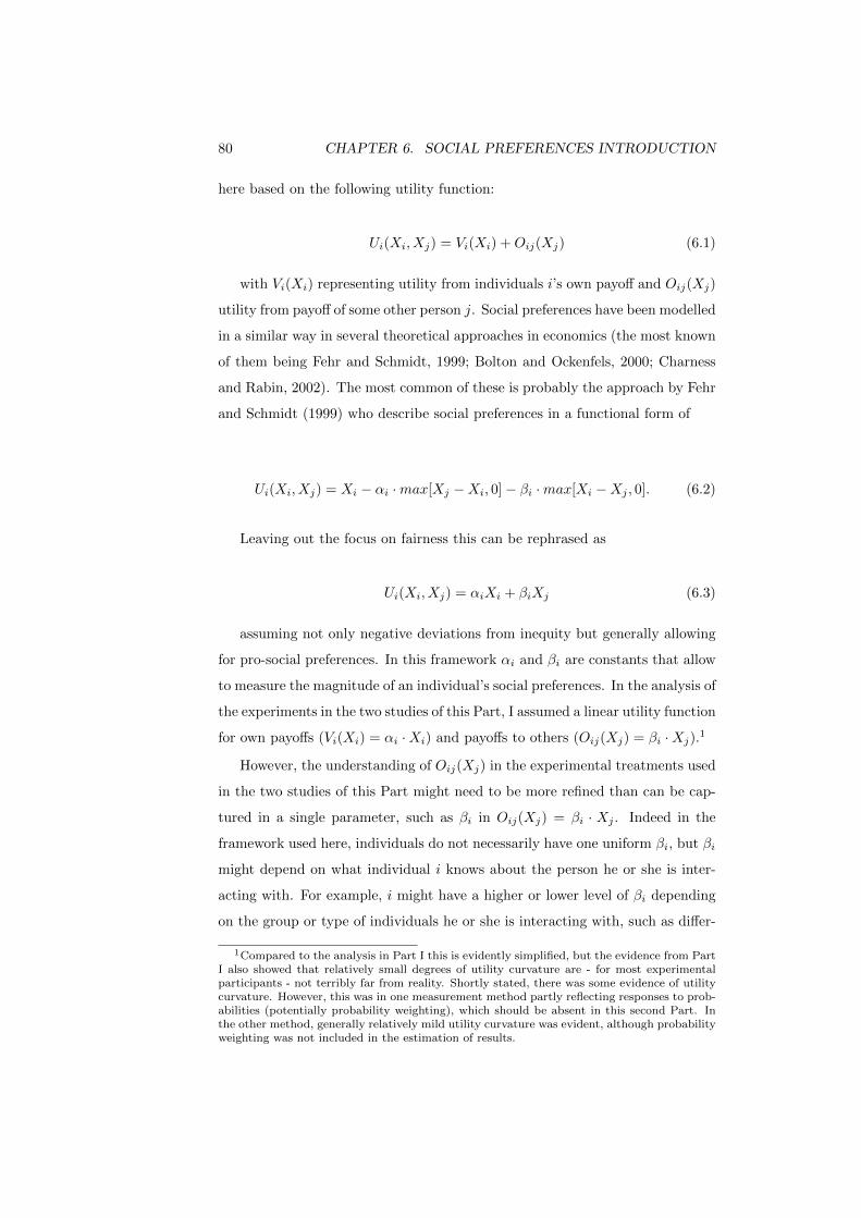
80 CHAPTER 6. SOCIAL PREFERENCES INTRODUCTION
here based on the following utility function:
Ui(Xi, Xj) = Vi(Xi) +Oij(Xj) (6.1)
with Vi(Xi) representing utility from individuals i’s own payoff and Oij(Xj)
utility from payoff of some other person j. Social preferences have been modelled
in a similar way in several theoretical approaches in economics (the most known
of them being Fehr and Schmidt, 1999; Bolton and Ockenfels, 2000; Charness
and Rabin, 2002). The most common of these is probably the approach by Fehr
and Schmidt (1999) who describe social preferences in a functional form of
Ui(Xi, Xj) = Xi − αi ·max[Xj −Xi, 0]− βi ·max[Xi −Xj , 0]. (6.2)
Leaving out the focus on fairness this can be rephrased as
Ui(Xi, Xj) = αiXi + βiXj (6.3)
assuming not only negative deviations from inequity but generally allowing
for pro-social preferences. In this framework αi and βi are constants that allow
to measure the magnitude of an individual’s social preferences. In the analysis of
the experiments in the two studies of this Part, I assumed a linear utility function
for own payoffs (Vi(Xi) = αi ·Xi) and payoffs to others (Oij(Xj) = βi ·Xj).1
However, the understanding of Oij(Xj) in the experimental treatments used
in the two studies of this Part might need to be more refined than can be cap-
tured in a single parameter, such as βi in Oij(Xj) = βi · Xj . Indeed in the
framework used here, individuals do not necessarily have one uniform βi, but βi
might depend on what individual i knows about the person he or she is inter-
acting with. For example, i might have a higher or lower level of βi depending
on the group or type of individuals he or she is interacting with, such as differ-
1Compared to the analysis in Part I this is evidently simplified, but the evidence from PartI also showed that relatively small degrees of utility curvature are - for most experimentalparticipants - not terribly far from reality. Shortly stated, there was some evidence of utilitycurvature. However, this was in one measurement method partly reflecting responses to prob-abilities (potentially probability weighting), which should be absent in this second Part. Inthe other method, generally relatively mild utility curvature was evident, although probabilityweighting was not included in the estimation of results.

6.1. INTRODUCTION 81
ent social preferences towards older or younger people, men or women, different
ethnicities, but also people with particular attitudes (e.g. List, 2006b, and refer-
ences therein). The common finding of “conditional cooperators”in public good
games (e.g. Kocher et al., 2008; Herrmann and Thoni, 2009; Thoni et al., 2012;
Fischbacher and Gachter, 2010) and of behaviour in gift exchange frameworks,
where kind actions by the counterpart are answered by more kind own actions,
sustain this view. Hence, βi could be understood as a function of the character-
istics of experimental counterparts. This aspect will be of particular importance
in the two studies in this Part.2
Hence, if experimental decisions of the counterparts allow to update informa-
tion about the type of the counterpart (such as beliefs over the level of kindness
of the other player) and once repeated decisions occur in experimental inter-
action, it might become reasonable to obfuscate or shade an own selfish type
or overstate own reciprocity for strategic reasons, e.g. by making more kind
offers. These actions would be such that the counterpart cannot (or at least
not fully) update beliefs about the true type of the player i. This consideration
is particularly central when investigating the difference between statistical and
taste-based discrimination in the second study of this Part.
The two studies in this Part describe experiments that investigate different
social preferences towards groups of people, or, in other words, discrimination
against a certain group; expressed formally, they study if βa and βb are different
between two groups of migrants (a) and locals (b). Furthermore, both studies
investigate the level of strategic decision-making, using two experimental games,
one in which strategic overstating makes sense, and one in which two decisions
comparable to the previously overstated decision can be made. In one the
incentive to overstate own kindness is increased, in the second it is eliminated.
As both experimental studies in this Part build on the same structure of using
two experimental games, the games are described in an introductory section
below, before describing the two studies and before their more specific research
2For example, if one would like to be more cooperative towards women then men, βwomeni >βmeni , where βxi , x ∈ [women,men] implies that the status of the counterpart in (experimentalor real) interaction is known and leads to changes in own decisions. Such notions of reciprocitythat conditions on the characteristics of the counterpart j have been modelled in more rigoroustheoretical frameworks, for example by Rabin (1993) or Dufwenberg and Kirchsteiger (2004).However, for understanding results in the studies presented here the simplified frameworkdescribed here should suffice.

82 CHAPTER 6. SOCIAL PREFERENCES INTRODUCTION
questions are addressed. To study these more specific questions as described in
the next section, the experiments in this Part use an interactive game structure
with two game variants that allow to measure different elements of βxi .
6.2 Aims of the following chapters
The first study of this Part investigates interaction between two different cul-
tural groups which are likely to interact in their future jobs. These groups are
native Australians and migrant Asians, mirroring a demographic trend in the
population structure in Australia where an increasing migrant Asian population
enters the labour market. As such, this is a topic with high policy relevance
due to its impact on the economic development of Australia. The experiment
investigates if the two groups behave differently as suggested by the literature
on cross-cultural experiments and if discrimination against Asians can be de-
tected.3 Furthermore, the study goes further into detail and investigates the de-
terminants of reciprocal decisions between the groups, finding that both groups,
despite their different cultural origin, behave similarly and that discrimination
against the migrant group is not observable. However, using the second game
structure indicates that the shape of social preferences is different depending
on whether Australians interact amongst themselves or with Asians. While the
overall level of reciprocity is similar for within- and cross-cultural interaction,
the social preference towards Australians is less dependent on the actions of their
experimental counterpart, while there is a significantly higher interactive reci-
procity (hence conditional kindness) towards Asians. At the same time Asians
are made promises which are just cheap talk, while promises to Australians play
a role for final decisions.
The second study in this Part takes its point of departure from observed
labour market discrimination in China. However, it is unclear what determines
the basis of discrimination and in particular which role policy plays. In this
study discrimination based on the hukou system is investigated, a policy seg-
regating Chinese citizens in groups of migrants and locals in urban China.4
3See the introduction to the chapter for a discussion of this literature.4Again see the discussion of discrimination towards the specific group of people in this
study for more detail and the underlying literature.
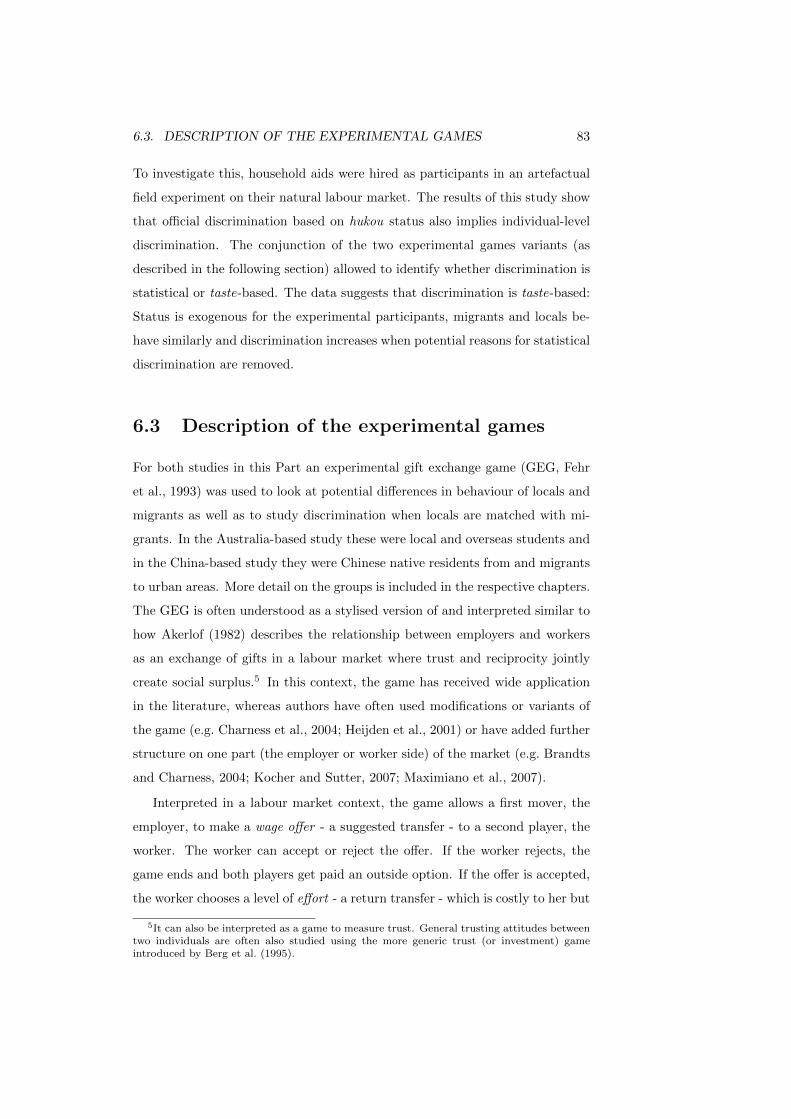
6.3. DESCRIPTION OF THE EXPERIMENTAL GAMES 83
To investigate this, household aids were hired as participants in an artefactual
field experiment on their natural labour market. The results of this study show
that official discrimination based on hukou status also implies individual-level
discrimination. The conjunction of the two experimental games variants (as
described in the following section) allowed to identify whether discrimination is
statistical or taste-based. The data suggests that discrimination is taste-based:
Status is exogenous for the experimental participants, migrants and locals be-
have similarly and discrimination increases when potential reasons for statistical
discrimination are removed.
6.3 Description of the experimental games
For both studies in this Part an experimental gift exchange game (GEG, Fehr
et al., 1993) was used to look at potential differences in behaviour of locals and
migrants as well as to study discrimination when locals are matched with mi-
grants. In the Australia-based study these were local and overseas students and
in the China-based study they were Chinese native residents from and migrants
to urban areas. More detail on the groups is included in the respective chapters.
The GEG is often understood as a stylised version of and interpreted similar to
how Akerlof (1982) describes the relationship between employers and workers
as an exchange of gifts in a labour market where trust and reciprocity jointly
create social surplus.5 In this context, the game has received wide application
in the literature, whereas authors have often used modifications or variants of
the game (e.g. Charness et al., 2004; Heijden et al., 2001) or have added further
structure on one part (the employer or worker side) of the market (e.g. Brandts
and Charness, 2004; Kocher and Sutter, 2007; Maximiano et al., 2007).
Interpreted in a labour market context, the game allows a first mover, the
employer, to make a wage offer - a suggested transfer - to a second player, the
worker. The worker can accept or reject the offer. If the worker rejects, the
game ends and both players get paid an outside option. If the offer is accepted,
the worker chooses a level of effort - a return transfer - which is costly to her but
5It can also be interpreted as a game to measure trust. General trusting attitudes betweentwo individuals are often also studied using the more generic trust (or investment) gameintroduced by Berg et al. (1995).
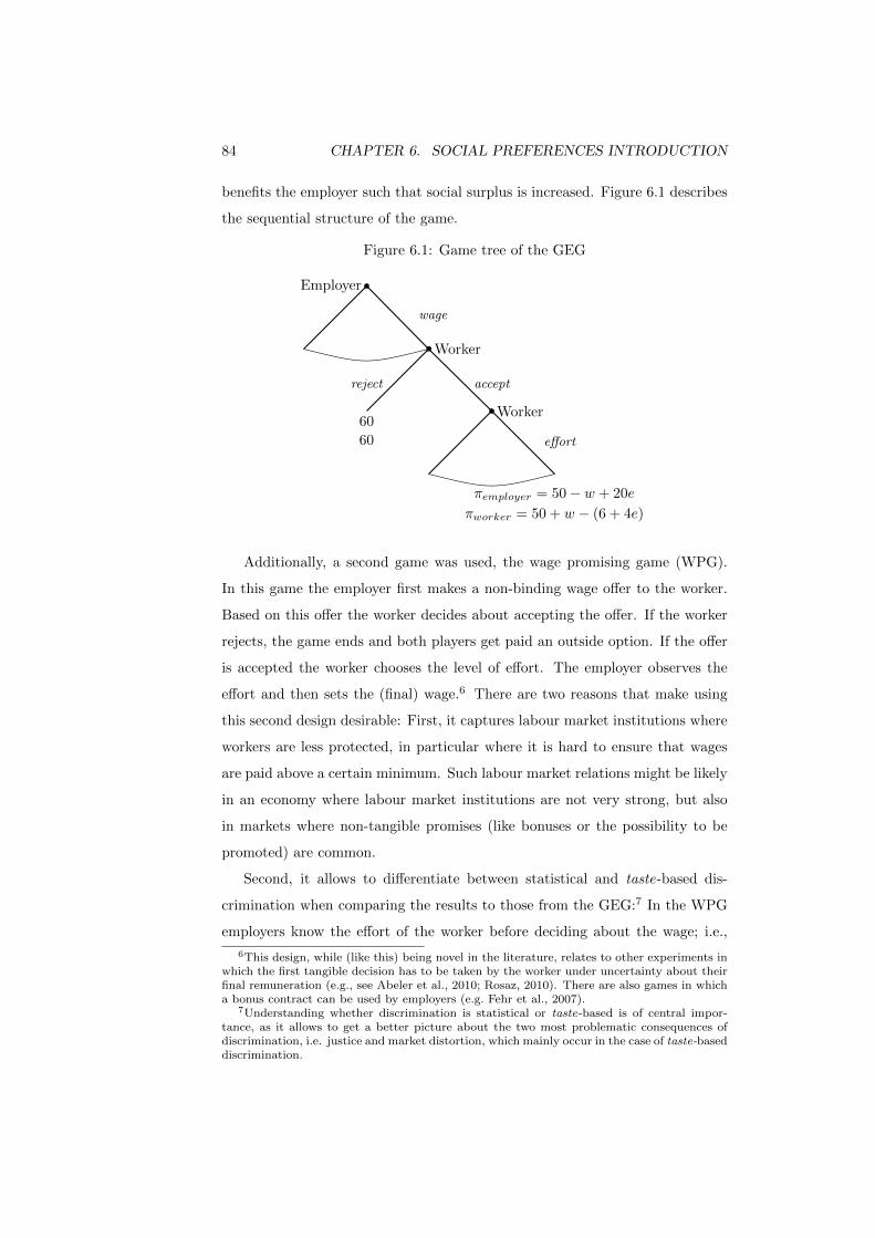
84 CHAPTER 6. SOCIAL PREFERENCES INTRODUCTION
benefits the employer such that social surplus is increased. Figure 6.1 describes
the sequential structure of the game.
Figure 6.1: Game tree of the GEG
Employer
Worker
Worker
wage
effort
reject accept
60
60
πemployer = 50− w + 20e
πworker = 50 + w − (6 + 4e)
Additionally, a second game was used, the wage promising game (WPG).
In this game the employer first makes a non-binding wage offer to the worker.
Based on this offer the worker decides about accepting the offer. If the worker
rejects, the game ends and both players get paid an outside option. If the offer
is accepted the worker chooses the level of effort. The employer observes the
effort and then sets the (final) wage.6 There are two reasons that make using
this second design desirable: First, it captures labour market institutions where
workers are less protected, in particular where it is hard to ensure that wages
are paid above a certain minimum. Such labour market relations might be likely
in an economy where labour market institutions are not very strong, but also
in markets where non-tangible promises (like bonuses or the possibility to be
promoted) are common.
Second, it allows to differentiate between statistical and taste-based dis-
crimination when comparing the results to those from the GEG:7 In the WPG
employers know the effort of the worker before deciding about the wage; i.e.,
6This design, while (like this) being novel in the literature, relates to other experiments inwhich the first tangible decision has to be taken by the worker under uncertainty about theirfinal remuneration (e.g., see Abeler et al., 2010; Rosaz, 2010). There are also games in whicha bonus contract can be used by employers (e.g. Fehr et al., 2007).
7Understanding whether discrimination is statistical or taste-based is of central impor-tance, as it allows to get a better picture about the two most problematic consequences ofdiscrimination, i.e. justice and market distortion, which mainly occur in the case of taste-baseddiscrimination.

6.3. DESCRIPTION OF THE EXPERIMENTAL GAMES 85
wages are not based on the workers expected effort (or trustworthiness, which
should only play a role as a decision variable in the GEG). The game structure
of the WPG is illustrated in Figure 6.2.
Figure 6.2: Game tree of the WPG
Employer
Worker
Worker
Employer
wage promise
effort
wage paid
reject accept
60
60
πemployer = 50− w + 20e
πworker = 50 + w − (6 + 4e)
In both studies a labour market framing, hence a description of the game
using these terms of employers, workers, wage offers, wage offer acceptance and
efforts were used. This made the game more understandable for participants,
but also limits the scope of potential interpretation of the results, as it framed
participants’ thinking to a labour market scenario. The payoff functions for
employers and workers were chosen to be reasonably simple and used values for
the level of wages that could be observed in a real labour market. I.e., wage
offers and final wages had to be between 5 and 100 experimental dollars and in
steps of 5. Returned efforts had to be between 1 and 10 in steps of 1 in case
the worker had accepted the wage offer. These decision variables and payoff
functions are similar to others in the literature (Gachter and Fehr, 2002). In
both games the payoff for the employer as well as for the worker in case the
worker rejected were πemployer = πworker = 60. In case the worker accepted,
the payoffs were (dependent on wages w and effort e):
πemployer = 50− w + 20e (6.4)

86 CHAPTER 6. SOCIAL PREFERENCES INTRODUCTION
and
πworker = 50 + w − (6 + 4e) (6.5)
Both games have a unique subgame perfect Nash equilibrium (in pure strate-
gies) in which both players receive the outside option: Wage payments will al-
ways be minimal as more than minimum effort, which is - out of equilibrium
- the best response of workers, cannot be enforced (GEG) or because they are
the optimal choice when paid ex post (WPG). Thus workers reject all offers.8
However, while this is the equilibrium in both games, previous experimental
evidence leads to the expectation of positive reciprocity in both games. Besides
preference to reciprocate, this behaviour may also stem from concerns for effi-
ciency – the mutual profit of employers and workers is increased by higher effort
of the worker. Gachter and Fehr (2002) provide an overview of a large part
of studies that make use of the GEG using various specifications. Similarly, in
the WPG it can also be conjectured that wage promises will be perceived as
relevant, at least if employers avoid lying in the signals they send (as in Gneezy,
2005). Furthermore, guilt aversion (Charness and Dufwenberg, 2006) might play
a role in decisions (but see Ellingsen et al., 2010): If employers feel guilty if they
promised high wages and only pay minimum ones, they will anticipate this and
both reduce the amount of their promises and orient their final wage decisions
closer on the promise. A similar effect could be due to positive surprises which
are more likely when low wage offers are made.
The comparison across the two games particularly makes sense when consid-
ering dynamic reciprocity as described above. In the GEG it can make sense for
employers to be strategically more reciprocal to workers in their wage offers and
to shade an own potential selfish type. The incentive to appear more reciprocal
further increases wage offers in the WPG, because in this game offers are not
binding; the shading motive disappears for final wage decisions in the WPG, as
there is no possibility to respond by the worker. Similarly, depending on the
importance of promises for final wage decisions, differences in feeling of guilt to-
8In the GEG wage offers above 10 are risky: If the worker accepts the offer and chooses theminimum effort (which is the least costly option for the worker), the employer would be worseoff than by getting the outside option. For workers in turn it is only (potentially) profitableto accept wage offers of 20 or more - even if they choose minimum effort. In the WPG wagepromises are just cheap talk, as they are not binding for final wage decisions. Any positiveeffort is hence risky for the worker compared to the safe option of rejecting.

6.3. DESCRIPTION OF THE EXPERIMENTAL GAMES 87
wards different groups can be studied. It is therefore hypothesised that (despite
the non-cooperative Nash equilibrium) individuals cooperate and reciprocate in
both games in terms of their tangible choices. It is further hypothesised that
(non-tangible) promises in the WPG play a role both for worker decisions and
for employer’s final wage decisions. More discussion of the strategic nature of
the variables is also included in the data appendices of the two chapters or
discussed and exemplified given the choices made by participants in the two
studies.
Finally, the structure of both games assumes that worker effort is (quantifi-
able and) observed by employers, a characteristic which is often not the case
in reality and a major source of principal-agent problems (see, for example,
Osborne and Rubinstein, 1994, for a discussion). However, this counterfactual
allows studying interesting elements of discrimination in the two approaches
included in the following.
In both studies these two games were played for 8 consecutive rounds each.
Participants received instructions for each game just before the first round of
each game (i.e., before rounds 1 and 9, respectively). Roles of workers and
employers were fixed throughout the experiment. In each of the 8 rounds pairs
of one worker and one employer were randomly rematched. From all 16 rounds,
4 rounds were randomly determined for final payoff. This was done to avoid
wealth effects in the course of the experiment and to make periods independent
in the sense that reputation-building should not play a role. Further procedural
details specific to the two studies are included in the descriptions of these studies.

88 CHAPTER 6. SOCIAL PREFERENCES INTRODUCTION

Chapter 7
Culture, trust and gift
exchange in an intercultural
labour market1
7.1 Introduction
The notion that people from different cultural backgrounds behave differently
from one another, particular when engaging in social interaction, is confirmed
by much anecdotal evidence and confirms many people’s daily observations
when dealing with someone from a different culture. Cultural differences in
behavioural patterns exist on many levels and on a gradual scale. They start
from slight differences between members of different families or people from ad-
jacent towns or villages to major cultural differences that are observable between
geographically distinct cultures such as Greeks and Chinese. Many of these dif-
ferences are based on social attitudes that are learned some way or another; i.e.
members of a cultural group usually learn about appropriate ways to interact
at home, school or simply through daily experience, shaping and maintaining
their behaviour in a culture-specific way.
The cultural knowledge about the own and outside groups results in differ-
1This chapter is based on collaborative work with Tony Beatton, Uwe Dulleck, and MarkusSchaffner.
89

90 CHAPTER 7. INTERCULTURAL SOCIAL PREFERENCES
ences of attitudes towards and of expectations about behaviour when interacting
with a different cultural group. This may be just based on accepted prejudice
about culture-specific characteristics, but is often not purely anecdotal. For ex-
ample, looking at and comparing cultures at a global level, Hofstede (2001) as
one of the most prominent examples gives structure to these differences and de-
velops a theoretical framework for understanding behavioural attitudes within
and between cultures.
Cultural differences have also been subject to scrutiny in terms of their eco-
nomic consequences. For example, variations in trust levels between countries
have been employed to explain differences in economic development and perfor-
mance between countries (Fukuyama, 1995; Knack and Keefer, 1997). However,
while these differences in cultural attitudes and values are quite certain to exist
on some level, it is not as clear that and, if so, in which way they impact eco-
nomic decisions. One channel of such behavioural differences could be different
distributions of social preferences within and between cultures (e.g. understood
in a theoretical framework as in Fehr et al., 1993; Bolton and Ockenfels, 2000;
Charness and Rabin, 2002, and with differences in β as described in the intro-
duction). For example, social preferences towards strangers could be stronger
in one country than in another. Similarly, the strength of social preferences
could be more or less dependent on the size of the group these preferences ex-
tend to. In societies in which family networks play an important role, social
preferences might be strong for family members, but weak for the wider society.
Inversely they might be less skewed for societies in which social networks are
less important in private matters and business relations.
Such patterns of social preferences between cultures could be used to explain
why culture-specific behaviour is observable. However, it is usually hard to
detect the culture-based preference patterns by just using observational data as
many unobservable effects confound the analysis. Therefore, using experiments
to study interaction of economic decision makers is a suitable and required
tool to investigate cultural differences and cross-cultural interaction. The role
of culture has consequently been studied in a large number of experimental
economic studies. Camerer (2003) provides a good overview of this literature,
covering result from the ultimatum bargaining game, the dictator game and

7.1. INTRODUCTION 91
the trust game. Some more recent studies (e.g. Ferraro and Cummings, 2007;
Bohnet et al., 2008) have further added to the literature.
Most of these cross-cultural studies compare the behaviour of culturally ho-
mogeneous subject groups, i.e. they study the behaviour of cultural groups in
their countries of origin. While many economic experiments have been con-
ducted involving participants of different cultural backgrounds, hence cross-
cultural studies, in particular in the context of the trust game (Croson and
Buchan, 1999; Holm and Danielson, 2005; Buchan et al., 2006; Ashraf et al.,
2006; Bohnet et al., 2008), much less work has been done involving interaction
between experimental participants from different cultural backgrounds, hence
intercultural studies.
Approaches that investigated intercultural interaction often employed the
strategy method, in which experimental participants in the recipient role specify
a (hypothetical) decision for every eventuality of game offers they might receive
(e.g. Walkowitz et al., 2005; Dakkak et al., 2007; Netzer and Sutter, 2009). In
these studies subjects in different locations around the globe described their
full intended behaviour and were informed that they will interact with partici-
pants from another culture. However, this allows for no direct communication
of choices back and forward between the groups and makes it more difficult
to interpret experimental results in terms of more direct (same-environment)
interaction between cultures. Furthermore, it is not as clear how likely these
groups of experimental participants are to interact in an intercultural context
in reality.
In the following analysis interaction of students that have a different cul-
tural origin, but live in the same country, was studied. These two groups were
Australian students and international students from Asia, a large group that
is likely to eventually migrate to Australia. To study intercultural interaction
between these two groups, an experimental labour market based on the gift ex-
change game (GEG) was used. Different cultural groups were identified using
a pre-experimental questionnaire that also provided information about trusting
attitudes of individuals.2 Trust, that is the willingness to put own outcomes in
the hand of others (or risk taking where the pro-social attitude of others is the
2As described with the results and discussed in more detail in the appendix, the question-naire can also be used to study selection into the experiment.

92 CHAPTER 7. INTERCULTURAL SOCIAL PREFERENCES
source of uncertainty), is understood as a major factor driving behaviour in the
GEG. In order to capture two different types of labour market contracts, the
experimental game was varied, using the GEG and WPG as described before.
The results of the study show that differences in (a) trusting attitudes and
behaviour as well as trustworthiness in the GEG are very similar across cultures,
making interaction between the cultural groups generally comparable. However,
it also shows that (b) interactions between the two cultures changed between
the two games. That is, there was no discrimination of Asian students in the
GEG with binding wage offers, but it can be observed that wage promises lose
their importance when made to Asians. This underlines the importance of the
institutional framework (which was modelled as an experimental game in this
study) for the interaction between cultures.
7.2 Intercultural trust and the labour market
A main aim of the study described in this chapter was to understand the in-
teraction between individuals from two culturally distinct groups who are likely
to interact in reality. Therefore, groups of Australian and Asian students were
identified who were not necessarily perfect representatives of their cultural group
of origin, but likely to migrate or interact with members of the other culture. For
this reason experimental participants were recruited in the Australian univer-
sity sector, which is characterised by a large number of international students,
a group likely to become the next generation of permanent migrants. Of these
international students a large fraction is Asian.3 The question of how the two
cultural groups interact is hence of high practical relevance. Furthermore, for
researchers interested in patterns of social interaction between individuals from
different cultures the Australian society is an interesting laboratory due to on-
going and dynamic immigration.
However, given theoretical considerations on cultural differences (as in Hof-
stede, 2001) and the experimental results from studies described in the intro-
3Australia is a country that, in a similar way to the United States, has a long and continuingtradition of immigration from different countries. For long periods immigration to Australia(and similarly to the USA) was based on migrants from mostly Western cultures that wereculturally similar to Australians. However, in more recent years migration patterns havechanged and immigrants are increasingly from Asian countries that have a different culturalbackground compared to Australia.

7.2. INTERCULTURAL TRUST AND THE LABOUR MARKET 93
duction, what patterns would be expected in interaction between Australians
(Westerners) and Asians (from Eastern cultures)? First answers to this can be
found in a study by Kuwabara et al. (2007) who investigate trusting behaviour
between Japanese and American students using trust games in an online lab-
oratory. They find differences between the two cultural groups and differences
between the cultures depending on whether participants are rematched. In
one-shot interaction American students are more trusting, in repeated interac-
tion the reverse result appears. In a study using domestic and international
students in Australia, Guillen and Ji (2011) find that (non-statistical) discrim-
ination against international students in the trust game is observable, which
in turn appears to lead to decreasing trust levels of the internationals over the
length of their stay in Australia.4 More precisely, their study finds insignificant
discrimination when looking at aggregate measures and significant discrimina-
tion once individual heterogeneity is taken into account. Hence, it seems that
culture matters for trusting decisions. It is therefore hypothesised that culture
has a significant influence on decisions of Australians, who might be discrimi-
nating against Asians. Partly as a response to this Asians might show different
patterns of reciprocity. Furthermore, it is hypothesised that the games change
the nature of interaction between the groups.
But why is trust between individuals from different cultures emphasised in
many studies (including the one in this chapter)? The first answer to this is that
the experimental and theoretical literature has identified trusting levels as an
area where individuals from Western and Eastern countries tend to differ. For
economists an important consideration is also to ask on which markets migrants
will have an impact in the country they arrive. For this it is useful to consider
the type of Asian migrants arriving in Australia. They are usually young, have
attained higher education and are aiming for at least middle-class jobs. In fact,
a major channel of Asian migration to Australia is via the tertiary education
system. Obtaining an Australian undergraduate or postgraduate degree, to-
gether with an employment opportunity, is seen as an entry ticket in terms of
visa regulations to stay in the country permanently. This has motivated a sig-
nificant number of Asian migrants to enrol in the Australian tertiary education
4Students in this study had been in Australia for a limited amount of time, usually lessthan five years.

94 CHAPTER 7. INTERCULTURAL SOCIAL PREFERENCES
system as a first step to migrate to the West. Hence, Asian student populations
at the university are likely to become permanent migrants. Once graduating
and leaving university (and potentially even before) these Asian migrants are
then likely to enter into the labour market, taking up jobs in which they are
employed by a local (Australian) company. The labour markets, particularly
those targeted by university graduates, as argued below, are markets in which
(employer-worker) trust is a major determinant of economic success.
Trust is important in this context as in many labour market situations em-
ployers ask workers to exert work effort which is not contractible ex ante or
verifiable ex post, at least not above some minimal level. If work effort is in
any way costly, workers that maximise their own benefit will hence never exert
more than minimal effort. However, only minimum effort is often not what
is observable in reality. In many cases employees work more than the mini-
mum specified in their contract. In response to this observation Akerlof (1982)
proposed the idea that such labour relationships are better understood as an
exchange of gifts. If employers pay more than minimum wages, these are per-
ceived as gifts by workers. This in turn induces workers to return a gift to the
employer through increased (non-enforceable) effort. Through this interaction,
positive reciprocity equilibria above the minimum pay-effort setting can evolve.
However, for such equilibria, the first mover (typically the employer paying an
above-minimum wage) has to have some trust into the worker’s willingness to
respond with more than minimum effort.
This idea is echoed in the experimental GEG, which models the relation-
ship between two players (employers and workers) as a mutual gift exchange
as described before. The main cornerstone of the gift exchange game is the
level of trust and social preferences (leading to reciprocal decisions) between
the involved players.
In the experiment used in this chapter the GEG and the WPG as described
before are used to implement labour market relationships between the cultural
groups. The WPG set-up was added to the GEG to reflect labour market
relationships in which employers make wage promises and pay wages ex post
and to see if including such a framework, which might be more typical for jobs of
highly qualified workers with an academic degree, would change the interaction

7.3. EXPERIMENTAL PROCEDURES 95
between the cultural groups.
7.3 Experimental procedures
7.3.1 Selection and invitation of participants
The central question of the experiment was to determine if cultural differences
would lead to different behaviour and different patterns of interaction in a labour
market situation. To study this, it was necessary to identify the cultural groups
so that they could interact in a controlled environment. For this the cultural
status of participants was identified before they came to the laboratory. Further-
more, some additional features, particularly the level of language comprehension
between the cultural groups had to be taken into account when studying the
interaction between the two cultural groups. The following paragraphs describe
the pre-experimental design and recruitment procedure.
In order to increase the control in the experiment, a questionnaire was used
which included information about cultural origin (asking for country of birth
and citizenship), length of stay in Australia (all of life or specifying years and
months), language proficiency, and various other questions, which are discussed
further below. Table 7.2 includes a list of attitudinal questions used in this
survey. Three further questions (culture, length of stay and language skills)
served as selection criteria by the experimenters. The main groups of interest
were Australians (who had lived there all their life) and Asians (more specifically
those from East and South-East Asia) in the student population; this second
group represents by far the largest cohort of international students at Australian
universities (see Australian Bureau of Statistics, 2007) and is perceived by much
of the resident Australian population as relatively homogeneous. Furthermore,
all these Asian students come from societies that are culturally quite distinct
from the Western culture in Australia.5
Evidently, however, there are always degrees of being a migrant and one
would expect cultural differences to diminish over time or at least conjecture
that migrants will adopt behavioural strategies that converge towards those of
5Evidently this group is also not entirely homogeneous and many Australians are aware ofthis. Nevertheless they are perceived as clearly culturally different, other than, for example,European immigrants.
96 CHAPTER 7. INTERCULTURAL SOCIAL PREFERENCES
the native population in the course of their stay (but see Guillen and Ji, 2011).
For this reason only students were invited that had only moved to Australia
relatively recently: They had to have moved after the age of 16 (increasing
the chances that they would have an accent when speaking English) and had
to have lived in Australia for less than 13 of their life. Practically, given that
mainly undergraduates in their first years were recruited for this study, most of
those identified as Asians were in their early 20s and had moved to Australia
less than 2 years before in order to so their university studies. As Australia
is a country with many Western migrants, some of which arrive in their early
childhood, Australian students were only selected when being born as Australian
(or New Zealand) citizens and who had ”lived in Australia all [their] life”, as
of the question in the survey. Hence, the definition included second-generation
migrants from any country (as of experimenter observations only one second-
generation Asian student participated – this was in a pure Australian session).
Furthermore, both groups had to answer an English proficiency test question
that asked them to understand a labour market situation. This was done to have
two groups in the experiment with comparable language and comprehension
skills. This allowed identifying groups who were (internally and between each
other) relatively homogeneous, but different in their cultural origin.
Furthermore, the questionnaire included information about work experience
of respondents, trust and social attitudes (such as religiousness, happiness or
workplace attitudes and experiences). Particularly trust, as it plays an impor-
tant role for decisions in the experimental (gift exchange) game, was of further
interest for this study. Participants were also asked for their consent of having
their e-mail address used for recruiting them for economic experiments.
The questionnaire was handed out to all students of the introductory eco-
nomics unit at the Queensland University of Technology over two years from
2010 to 2011 in the beginning of each teaching period (3 times per year). Ap-
proximately 3000 questionnaires were handed out in paper form in the first
weeks, which led to an almost complete coverage of the students. Additionally,
in the first teaching period of 2012, the questionnaire was provided online and
all students were made aware of this. From these, 2475 questionnaires were
returned completed, allowing to select students into the study. If students that

7.3. EXPERIMENTAL PROCEDURES 97
Tab
le7.
1:A
ttit
udin
al
elem
ents
inp
re-e
xp
erim
enta
lqu
esti
on
nair
e
Ple
ase
an
swer
thes
equ
esti
on
sw
hic
hask
ab
ou
ttr
ust
inoth
ers:
T1
Ind
ealin
gw
ith
stra
nger
s,it
isb
ette
rto
be
cau
tiou
su
nti
lth
eyh
ave
pro
vid
edev
iden
ceth
at
they
are
tru
stw
ort
hy
T2
Most
peo
ple
kee
pth
eir
pro
mis
esT
3M
ost
peo
ple
an
swer
qu
esti
on
sh
on
estl
yT
4M
ost
peo
ple
say
wh
at
they
bel
ieve
them
selv
esan
dn
ot
wh
at
they
thin
kyou
want
toh
ear
T5
Most
peo
ple
tell
the
tru
thab
ou
tth
elim
its
of
thei
rkn
ow
led
ge
T6
Most
peo
ple
can
not
be
cou
nte
don
tod
ow
hat
they
say
they
will
do
T7
Th
ese
days,
you
mu
stb
eale
rtor
som
eon
eis
likel
yto
take
ad
vanta
ge
of
you
T8
In
orm
all
yre
lyon
the
task
-rel
ate
dsk
ills
an
dab
ilit
ies
of
oth
ers
T9
Iw
ou
ldn
ot
follow
the
ad
vic
eof
oth
ers
on
imp
ort
ant
issu
esT
10
Ico
nfi
den
tly
allow
oth
erp
eop
leto
make
dec
isio
ns
for
me
du
rin
gan
ab
sen
ceT
11
Iw
ou
ldre
lyon
task
-rel
ate
dju
dgem
ents
mad
eby
oth
ers
T12
Iu
sually
mon
itor
oth
ers
wh
enth
eyh
ave
tod
oso
met
hin
gfo
rm
e
Ple
ase
thin
kof
an
idea
ljo
b,
dis
regard
ing
you
rp
rese
nt
job
,if
you
have
on
e.In
choosi
ng
an
idea
ljo
b,
how
imp
ort
ant
wou
ldit
be
toyou
to..
.C
1h
ave
suffi
cien
tti
me
for
you
rp
erso
nal
or
hom
elife
C2
have
ab
oss
(dir
ect
sup
erio
r)you
can
resp
ect
C3
get
reco
gn
itio
nfo
rgood
per
form
an
ceC
4h
ave
secu
rity
of
emp
loym
ent
C5
have
ple
asa
nt
peo
ple
tow
ork
wit
hC
6d
ow
ork
that
isin
tere
stin
gC
7b
eco
nsu
lted
by
you
rb
oss
ind
ecis
ion
sin
volv
ing
you
rw
ork
C8
live
ina
des
irab
leare
aC
9h
ave
ajo
bre
spec
ted
by
you
rfa
mil
yan
dfr
ien
ds
C10
have
chan
ces
for
pro
moti
on
...c
onti
nu
ati
on
on
nex
tp
age
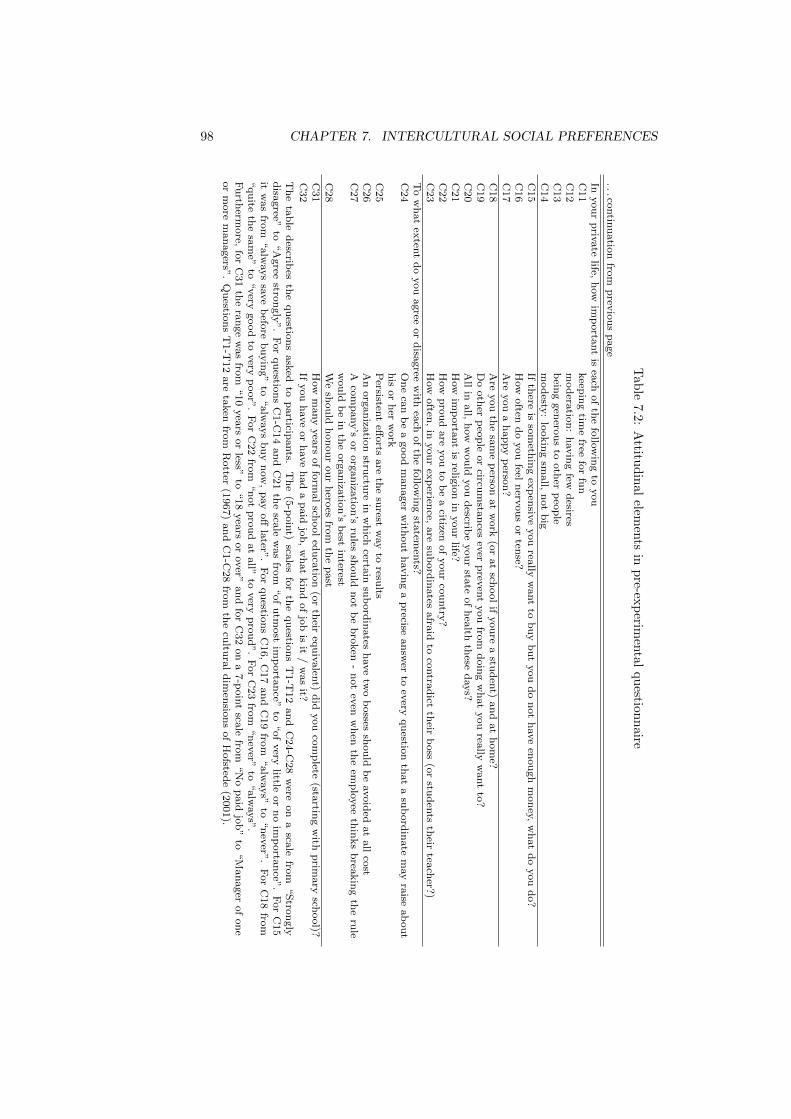
98 CHAPTER 7. INTERCULTURAL SOCIAL PREFERENCEST
able
7.2
:A
ttitud
inal
elemen
tsin
pre-ex
perim
enta
lqu
estionn
aire
...contin
uatio
nfro
mp
revio
us
page
Inyou
rp
rivate
life,h
ow
imp
orta
nt
isea
chof
the
follo
win
gto
you
C11
keep
ing
time
freefo
rfu
nC
12
mod
eratio
n:
havin
gfew
desires
C13
bein
ggen
erou
sto
oth
erp
eop
leC
14
mod
esty:
lookin
gsm
all,
not
big
C15
Ifth
ereis
som
ethin
gex
pen
sive
you
really
want
tob
uy
bu
tyou
do
not
have
enou
gh
mon
ey,w
hat
do
you
do?
C16
How
often
do
you
feeln
ervou
sor
tense?
C17
Are
you
ah
appy
perso
n?
C18
Are
you
the
sam
ep
erson
at
work
(or
at
school
ifyou
rea
stud
ent)
an
dat
hom
e?C
19
Do
oth
erp
eop
leor
circum
stan
cesev
erp
reven
tyou
from
doin
gw
hat
you
really
want
to?
C20
All
inall,
how
wou
ldyou
describ
eyou
rsta
teof
hea
lthth
esed
ays?
C21
How
imp
orta
nt
isrelig
ion
inyou
rlife?
C22
How
pro
ud
are
you
tob
ea
citizenof
you
rco
untry
?C
23
How
often
,in
you
rex
perien
ce,are
sub
ord
inates
afra
idto
contra
dict
their
boss
(or
stud
ents
their
teach
er?)
To
wh
at
exten
td
oyou
agree
or
disa
gree
with
each
of
the
follo
win
gsta
temen
ts?C
24
On
eca
nb
ea
good
man
ager
with
ou
th
avin
ga
precise
an
swer
toev
eryqu
estion
that
asu
bord
inate
may
raise
ab
ou
th
isor
her
work
C25
Persisten
teff
orts
are
the
surest
way
toresu
ltsC
26
An
org
an
izatio
nstru
cture
inw
hich
certain
sub
ord
inates
have
two
bosses
shou
ldb
eavoid
edat
all
cost
C27
Aco
mp
any’s
or
org
an
izatio
n’s
rules
shou
ldn
ot
be
bro
ken
-n
ot
even
wh
enth
eem
plo
yee
thin
ks
brea
kin
gth
eru
lew
ou
ldb
ein
the
org
an
izatio
n’s
best
interest
C28
We
shou
ldh
on
ou
rou
rh
eroes
from
the
past
C31
How
many
yea
rsof
form
al
school
edu
catio
n(o
rth
eireq
uiv
alen
t)d
idyou
com
plete
(startin
gw
ithp
rimary
school)?
C32
Ifyou
have
or
have
had
ap
aid
job
,w
hat
kin
dof
job
isit
/w
as
it?
Th
eta
ble
describ
esth
equ
estion
sask
edto
particip
ants.
Th
e(5
-poin
t)sca
lesfo
rth
equ
estion
sT
1-T
12
an
dC
24-C
28
were
on
asca
lefro
m“S
tron
gly
disa
gree”
to“A
gree
stron
gly
”.
For
qu
estion
sC
1-C
14
an
dC
21
the
scale
was
from
“of
utm
ost
imp
orta
nce”
to“of
very
littleor
no
imp
orta
nce”
.F
or
C15
itw
as
from
“alw
ays
save
befo
reb
uyin
g”
to“alw
ays
bu
yn
ow
,p
ay
off
later”
.F
or
qu
estion
sC
16,
C17
an
dC
19
from
“alw
ays”
to“n
ever”
.F
or
C18
from
“qu
iteth
esa
me”
to“very
good
tovery
poor”
.F
or
C22
from
“n
ot
pro
ud
at
all”
tovery
pro
ud
”.
For
C23
from
“n
ever”
to“alw
ays”
.F
urth
ermore,
for
C31
the
ran
ge
was
from
“10
yea
rsor
less”to
“18
yea
rsor
over”
and
for
C32
on
a7-p
oin
tsca
lefro
m“N
op
aid
job
”to
“M
an
ager
of
on
eor
more
man
agers”
.Q
uestio
ns
T1-T
12
are
taken
from
Rotter
(1967)
an
dC
1-C
28
from
the
cultu
ral
dim
ensio
ns
of
Hofsted
e(2
001).

7.3. EXPERIMENTAL PROCEDURES 99
filled out the questionnaire had indicated they would be willing to participate
in economic experiments (this was one question included at the end of the sur-
vey), the information required for this experiment was included into ORSEE
(Greiner, 2004), which was subsequently used for recruitment. Based on the
eligibility criteria (cultural background, language ability and consent to partic-
ipate in experiments) 1829 participants were invited to the laboratory.
The time distance between collecting the questionnaire and the experiment
was usually several weeks to reduce the problem of an influence of the ques-
tionnaire on experimental decisions. Based on these invitations, 172 students
came to the lab and 154 participated in the experiment. The appendix includes
more information on who participated and how the selection process might have
influenced decisions.6
7.3.2 Experimental implementation
At the start of the experiment, the first game was described to the partici-
pants and the roles of workers and employers were assigned. Instructions were
read out by a native English speaker and participants were asked to follow
the instructions which were also displayed on their computer screens. For the
investigation of differences between Australians and Asian migrants two treat-
ments were used. In the first scenario, Australian participants played among
each other. In the second scenario, Australians were assigned the role of the
employer and Asians the role of the worker. The rationale for this was that,
particularly in the early years of the employment history of Asians, this is the
most likely scenario in a real labour market where migrants are in the worker
role hired by local companies. For this second treatment an additional sentence
was used when reading out the instructions:
“Please note that in today’s session the roles have been assigned such that
the role of the worker has always been assigned to a foreign born person, more
specifically an Asian-born person, and the role of the employer has always been
assigned to an Australian-born person.”
While participants were unable to observe decisions on the computer screens
6In short, some non-experimenter-induced selection into the experiment is observable, how-ever, there should be no significant impact on the results reported in the following.

100 CHAPTER 7. INTERCULTURAL SOCIAL PREFERENCES
of others, they were able to observe the credibility of this claim based on the
fact that half of the laboratory was occupied by Asian and the other half by
Australian students. Hence, anonymity of decisions was preserved while the
instructions were credible. The experimental games were described in a labour
market framing. Participants were informed about potential earnings in the
experiment and the exchange rate between experimental and Australian dollars
of “100 experimental dollars = 5 Australian dollars”in the beginning of the
experiment.
All students proceeded through 8 rounds of each game, playing the GEG first
and the WPG second (hence one session consisted of 16 rounds). This design
does not allow to test for game order effects, which may be present. However,
there should be no interaction effect between game order and the treatment
driving the differences studied here. While they received feedback about the
outcomes in each round, they only learned about their final payoff based on 4
randomly determined rounds at the end of the experiment. Participants earned
on average about 20 Australian dollars during the experiment, which typically
lasted for about 1 hour, which included seating participants, the experiment
itself and a short post-experimental questionnaire.
Finally, some calculated drop-outs as well as unintended mistakes in the
implementation of the experiment should be mentioned. One calculated effect
was that due to the fact that 4 Australians and 4 Asians were required for
running an intercultural session significant overbooking was necessary, leading
to a noticeable number of individuals being sent home after paying them a
show-up fee. There was also a mistake in seating individuals in one session
(some Asians sat on computers that were giving them the employer role); this
session had to be dropped.
Finally, during some sessions participants were accidentally invited for a
second time to the experiment; these sessions were nevertheless included in the
analysis, but the impact of the potential double participants was scrutinised us-
ing several robustness checks. In total, 9 participants and 3 sessions (in which
repeated participants were present) were affected. Participants were in different
roles and treatments across participations which required an almost case-by-case
analysis of decisions. The appendix includes information about these partici-

7.4. RESULTS OF THE PRE-EXPERIMENTAL QUESTIONNAIRE 101
pants and reports results from various robustness checks, indicating that it is
acceptable to include the double participants in the analysis. To shortly sum-
marise, the robustness checks comprised of the exclusion of the second-time
participants from the sample as well as an analysis of observable changes in
decision patterns from the first to the second participation. The exclusion did
not lead to qualitative changes in the results, and any measurable changes (such
as changes in the significance levels) are reported in the following. With respect
to changes in behaviour accross the two participations, there might be more
cooperation observable in the second participation. However, this effect does
not appear to be different across treatments and does not seem to drive any of
the results reported in the following.
7.4 Results of the pre-experimental questionnaire
7.4.1 General elements of the questionnaire
The primary purpose of the questionnaire was to identify the cultural origin of
participants and to select two distinct groups that could meaningfully be com-
pared in an experiment. The questionnaire data supports the original conjecture
that the student population at the university where the study was conducted was
dominated by two populations, Australians and migrants from East and South-
East Asia, while migrants from other, various backgrounds take a small fraction
in the overall distribution. Figure 7.1 documents this observation. Students
were allocated to the categories of Australians, East Asians (covering Asia and
South-East Asia from China eastwards to Japan and southwards to Indonesia),
Central Asians (from Afghanistan to the middle East), Indians (India, Pakistan,
Sri Lanka and Bangladesh), Africans, Europeans (including Russia) and Ameri-
cans (North and South combined) as well as South Sea Islanders (countries such
as Papua New Guinea, Fiji, Tonga, etc.).
The pre-experimental questionnaire provided information about various other
demographics and attitudes of the student subject pool. As the questionnaire
was handed out to many students in the beginning of the semester, it provides
not only information about individuals that finally participated in the experi-
ment. It also includes information about those that were generally willing to

102 CHAPTER 7. INTERCULTURAL SOCIAL PREFERENCES
Figure 7.1: Countries of origin of questionnaire respondents
Australian East and Southeast Asian
Indian European
American African
Pacific Islander Central Asian
participate in experiments, but did not come to any of the sessions, as well as
about students that filled out the questionnaire, but were not willing to be ex-
perimental participants. Consequently, it can be investigated who was willing
to participate in sessions, who came and participated, and if participants were
representative of the overall student population studied. As understanding dif-
ferences between the two groups of Australians and Asians was a major goal in
this study, potential cultural differences can be investigated using the observa-
tional data from the questionnaire, which further adds to the information on
choices in the experiment.
In a further step, also the influence of any attitudes recorded in the ques-
tionnaire could be linked to decisions in the experiment, although the matching
of pre-experimental answers to experimental choices could not be achieved for
every participant.7 The importance of potential selection into the experiment
based on a number of characteristics, as well as the impact of any differences
between the two cultural groups in their attitudes on experimental decisions
could be studied. The following paragraphs describe the main features of the
7For 4 participants the participants number was not matched to the email address whenrunning the sessions, other participants changed their email address in the ORSEE databaseand could not be matched to their pre-experimental questionnaire any more.
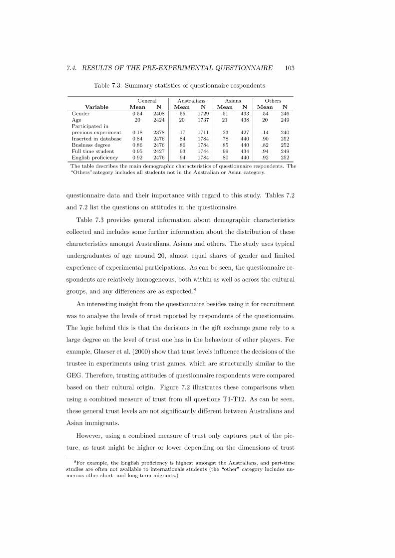
7.4. RESULTS OF THE PRE-EXPERIMENTAL QUESTIONNAIRE 103
Table 7.3: Summary statistics of questionnaire respondents
General Australians Asians OthersVariable Mean N Mean N Mean N Mean N
Gender 0.54 2408 .55 1729 .51 433 .54 246Age 20 2424 20 1737 21 438 20 249Participated inprevious experiment 0.18 2378 .17 1711 .23 427 .14 240Inserted in database 0.84 2476 .84 1784 .78 440 .90 252Business degree 0.86 2476 .86 1784 .85 440 .82 252Full time student 0.95 2427 .93 1744 .99 434 .94 249English proficiency 0.92 2476 .94 1784 .80 440 .92 252
The table describes the main demographic characteristics of questionnaire respondents. The“Others”category includes all students not in the Australian or Asian category.
questionnaire data and their importance with regard to this study. Tables 7.2
and 7.2 list the questions on attitudes in the questionnaire.
Table 7.3 provides general information about demographic characteristics
collected and includes some further information about the distribution of these
characteristics amongst Australians, Asians and others. The study uses typical
undergraduates of age around 20, almost equal shares of gender and limited
experience of experimental participations. As can be seen, the questionnaire re-
spondents are relatively homogeneous, both within as well as across the cultural
groups, and any differences are as expected.8
An interesting insight from the questionnaire besides using it for recruitment
was to analyse the levels of trust reported by respondents of the questionnaire.
The logic behind this is that the decisions in the gift exchange game rely to a
large degree on the level of trust one has in the behaviour of other players. For
example, Glaeser et al. (2000) show that trust levels influence the decisions of the
trustee in experiments using trust games, which are structurally similar to the
GEG. Therefore, trusting attitudes of questionnaire respondents were compared
based on their cultural origin. Figure 7.2 illustrates these comparisons when
using a combined measure of trust from all questions T1-T12. As can be seen,
these general trust levels are not significantly different between Australians and
Asian immigrants.
However, using a combined measure of trust only captures part of the pic-
ture, as trust might be higher or lower depending on the dimensions of trust
8For example, the English proficiency is highest amongst the Australians, and part-timestudies are often not available to internationals students (the “other” category includes nu-merous other short- and long-term migrants.)

104 CHAPTER 7. INTERCULTURAL SOCIAL PREFERENCES
Figure 7.2: Aggregated trust levels of questionnaire respondents
10
20
30
40
50
Tru
st
Africa
n
Amer
ican
Austra
lian
Cen
tral A
sian
East A
sian
Europ
ean
Indian
Pacific Island
er
investigated in the 12 questions.9 As can be seen in Table 7.4, significant dif-
ferences between many of the variables exist between the groups of Australians
and Asians, but these differences are washed out when creating a combined
measure. This statement is apparent when comparing the trust questions for
all Australians and Asians that answered the questionnaire (here Asians were
significantly more trusting based on variables T4, T5, T8 and T12, but signif-
icantly less trusting based on variables T1, T3, T6, T7, T9 and T11). Similar
switching between more and less trusting depending on the variables looked
at can also be observed for those Australians and Asians who participated in
experimental sessions. For this reason in later analysis it was checked if the
singular variables had any significant influence on experimental decisions.
Using the questionnaire, further information was recorded on other attitudes
as documented in Table 7.2. Generally, there were significant differences between
the Australian respondents and respondents from other regions; however, these
differences were usually region-specific. Individuals from regions such as Africa
as compared to India did not show the same differences when being compared
to Australians. The directions of these differences are mainly as expected and
9Hence looking at each question T1-T12 separately instead of using Trust(combined)=
∑12i=1 |Ti|.
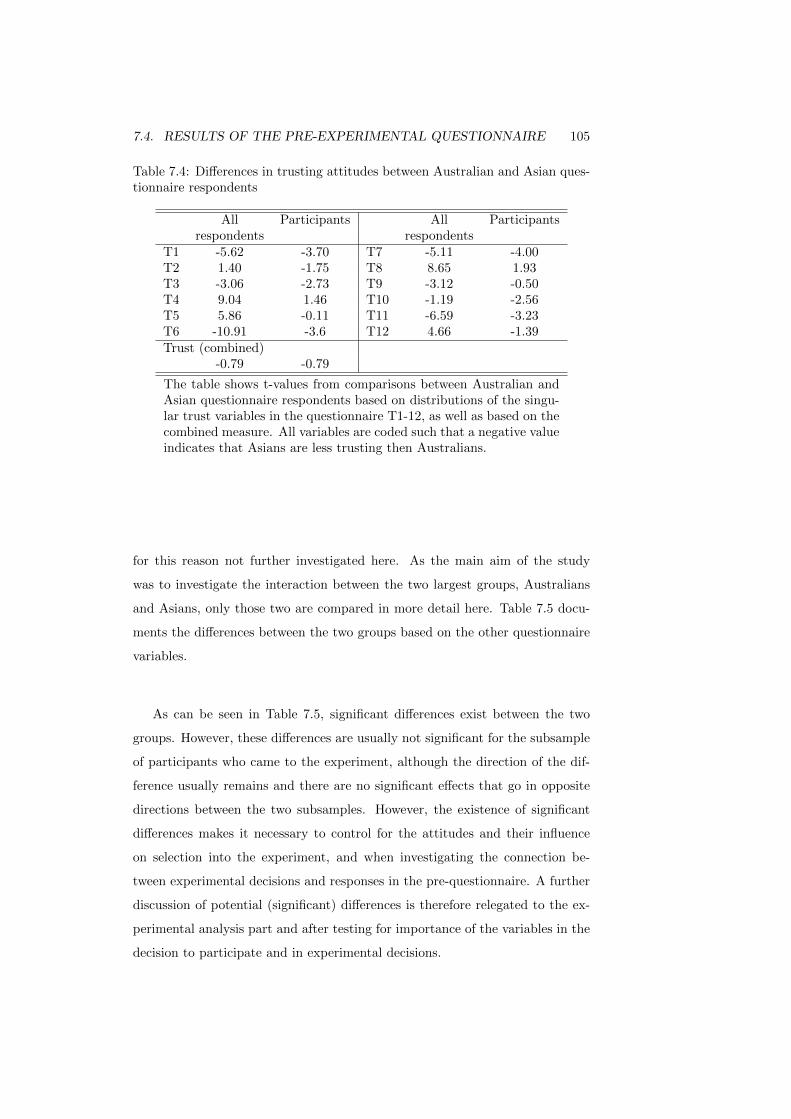
7.4. RESULTS OF THE PRE-EXPERIMENTAL QUESTIONNAIRE 105
Table 7.4: Differences in trusting attitudes between Australian and Asian ques-tionnaire respondents
All Participants All Participantsrespondents respondents
T1 -5.62 -3.70 T7 -5.11 -4.00T2 1.40 -1.75 T8 8.65 1.93T3 -3.06 -2.73 T9 -3.12 -0.50T4 9.04 1.46 T10 -1.19 -2.56T5 5.86 -0.11 T11 -6.59 -3.23T6 -10.91 -3.6 T12 4.66 -1.39Trust (combined)
-0.79 -0.79
The table shows t-values from comparisons between Australian andAsian questionnaire respondents based on distributions of the singu-lar trust variables in the questionnaire T1-12, as well as based on thecombined measure. All variables are coded such that a negative valueindicates that Asians are less trusting then Australians.
for this reason not further investigated here. As the main aim of the study
was to investigate the interaction between the two largest groups, Australians
and Asians, only those two are compared in more detail here. Table 7.5 docu-
ments the differences between the two groups based on the other questionnaire
variables.
As can be seen in Table 7.5, significant differences exist between the two
groups. However, these differences are usually not significant for the subsample
of participants who came to the experiment, although the direction of the dif-
ference usually remains and there are no significant effects that go in opposite
directions between the two subsamples. However, the existence of significant
differences makes it necessary to control for the attitudes and their influence
on selection into the experiment, and when investigating the connection be-
tween experimental decisions and responses in the pre-questionnaire. A further
discussion of potential (significant) differences is therefore relegated to the ex-
perimental analysis part and after testing for importance of the variables in the
decision to participate and in experimental decisions.

106 CHAPTER 7. INTERCULTURAL SOCIAL PREFERENCES
Table 7.5: Differences in attitudes between Australian and Asian questionnairerespondents
All Participants All Participantsrespondents respondents
C1 0.63 0.65 C15 2.09 -1.00C2 5.96 0.88 C16 -3.73 -1.83C3 -0.08 -2.55 C17 5.14 0.56C4 2.00 0.01 C18 7.61 0.31C5 -3.70 0.57 C19 -2.13 0.79C6 1.45 -0.53 C20 8.39 -0.45C7 5.52 0.45 C21 -6.56 -4.27C8 0.10 -1.19 C22 -6.14 -2.17C9 -4.78 -1.45 C23 -9.01 0.17C10 2.29 -1.07 C24 -11.01 -2.49C11 3.04 1.18 C25 -6.78 -0.83C12 -9.71 -3.62 C26 2.32 3.05C13 -1.62 -0.30 C27 2.08 0.01C14 -3.28 -0.74 C28 -3.65 -2.06
The table shows t-values for comparisons between Australian andAsian respondents in the pre-experimental questionnaire based ondistributions of the variables C1-C28. A positive value signifies thatthe value was higher for Australians. The interpretation of the coef-ficient is dependent on the scale of the question as described in Table7.2.

7.4. RESULTS OF THE PRE-EXPERIMENTAL QUESTIONNAIRE 107
7.4.2 Selection into the experiment and experimental de-
cisions
Given the large amount of questionnaire respondents, it was also possible to
investigate selection into the experiment and how this might have influenced
experimental decisions. A detailed analysis of these questions is included in
the appendix. Summarising the analysis in the appendix, some selection into
the experiment can be observed. Table 7.6 summarises the intended and unin-
tended selection effects, showing that on the first two selection steps, i.e. for the
database subscription and experimenter-induced selection (based on language
proficiency and cultural origin), the global selection effect is small.
Table 7.6: Experimental selection
Selection effect
1st step: Subscription to the database (84% of questionnaire respondentsdid so)
• For Australians: Main effect on non-subscription through part-time students (selection regression with a highest R2
adj ≈ .02)
• For Asians: Main effect on non-subscription through language pro-ficiency (selection regression with R2
adj ≈ .06)
2nd step: Experimenter-induced selection of cultural groups and of indi-viduals with sufficient language proficiency (88% of database subscriberswere invited)
3rd step: Registration and appearance for experimental sessions (7% ofquestionnaire respondents)
• For Australians: Main effect on participation through part-timestudents and language ability (selection regression with highestR2adj ≈ 0.2)
• For Asians: Main effect on participation through language abil-ity and questionnaire variables C18, C21, C26 (tracked throughfurther analysis, see appendix) (selection regression with highestR2adj ≈ .1)
In the third selection step, the decision to participate in the experiment the
sample reduces significantly; again, however, there does not seem to be a strong

108 CHAPTER 7. INTERCULTURAL SOCIAL PREFERENCES
(undesired) selection effect in this step (see appendix for details). Hence, this
selection does not seem to be undesired in the sense that it would lead to a
non-representative student population, as the effect of any undesired selection
into the experiment is (economically) small. Finally, one might ask if selection
into the experiment shifts experimental results in any way. As outlined in more
detail in the appendix, there is some selection effect for Australians which might
impact decisions. For Australians this selection goes through the trusting vari-
able T3 (which has a counterintuitive effect); for wage offers there is, however,
no effect on the treatment and the effect through this variable on final wages
does not shift results such that the conclusions need to be revised (again, this
is argued at more length in the appendix). As a result, there does not seem
to be a result-distorting selection effect and the conclusions from the analysis
presented in the following sections should remain.
7.5 Experimental Decisions
Given the design of the experiment, one main treatment variable was used,
i.e. sessions were done with either only Australians in the laboratory or with
Australian employers and Asian workers. I will also refer to these two treat-
ments as the Australian group and the intercultural group in the following. The
comparison of decision patterns across treatments, however, takes a different
interpretation depending on whether the employer or the worker role is stud-
ied. When looking at employer decisions potential discrimination is studied,
hence changes of decision patterns based on a characteristic of the experimental
counterpart. In terms of the overall framework of thinking this could be seen
as focussing on βji and studying its dependence on what is known about my
counterpart who will receive Xj .
When looking at worker decisions, in contrast, the interpretation of deci-
sions is somewhat different. As the characteristic of the counterpart is always
Australian, differences in behavioural patterns across treatments are based on
own characteristic or identity. Again, stated in the framework of thinking, the
focus is on αi and its dependence on a individual’s characteristic(s). Reflecting
this different interpretation of the treatment variable, in the following sections

7.5. EXPERIMENTAL DECISIONS 109
employer and worker decisions are described and analysed separately (while
recognising their reciprocal connections). However, before proceeding to the
more detailed analysis, some general features about the data, which are only
peripherally discussed in the analysis of the choice variables and which play a
role for both employers and workers, are described in the following paragraphs.
Firstly, as mentioned in the procedures section, some individuals accidentally
were allowed to participate in the experiment twice (the double participants).
Generally, there is nothing inherently wrong when letting a participant come
to the experiment twice, particularly when the time between the sessions was
long enough (as in our case it was in some cases more than one year). There-
fore, participants were most likely not reacting to their previous experimental
experience. For the double participants no noticeable change in behaviour be-
tween the first and the second session was observable. However, counting the
decisions of these individuals twice might distort the overall result if the double
participants are a special selection of the subject pool. Furthermore, if they
behave exactly the same between sessions, they might even drive overall results.
These possibilities were tested for by doing the analysis using two samples: one
sample uses both first and second participation decisions of these individuals,
the other just the first one. Results from this procedure show that there are
no qualitative changes due to using the double individuals and if there were
slight changes in the significance levels reported in the main analysis, these are
mentioned in footnotes.
Another general point relating to both employer and worker decisions is the
influence of demographic variables that were collected in the post-experimental
questionnaire. None of the demographic variables such as income, gender or
happiness had a clear and significant impact on the decision variables. Addi-
tionally, the post-experimental questionnaire also collected further information
about general trusting attitudes, which were argued to have an influence on
decisions in the gift exchange game. These variables had an influence on some
of the decision variables with the expected signs and in a statistically significant
way. There were some differences between the two treatments and although
confirming general conjectures about the intuition of the games with respect
to trust, they added no further insight beyond what is discussed in the ap-

110 CHAPTER 7. INTERCULTURAL SOCIAL PREFERENCES
pendix about the influence of answers in the pre-experimental questionnaire.
Furthermore, as the post-experimental questionnaire asked trust questions after
decisions were made, the causal direction is not clear and might even reflect
ex-post justification of decisions. For this reason, no further detail is included
here.
There are further general aspects about the data to consider. One is a
potential time trend in decisions, as in the experiment decisions were made
over several rounds. Indeed, time trends seem to be observable for all of the
decision variables with a tendency to reverse the time trend in later periods
(hence the variable period and period2 have opposite effects). However, the
economic significance of these time trends is small for both groups and games,
as shown in Figures 7.3, 7.4 and 7.5. Furthermore, the significance of time
trends disappears once regressions allowed for reciprocal patterns between own
decisions and those of others in previous periods.
Figure 7.3: Development of wage offers over the rounds
05
01
00
05
01
00
0 2 4 6 8 0 2 4 6 8
WPG, Australians only WPG, Intercultural group
GEG, Australians only GEG, Intercultural group
95% CI Fitted values Wage offer
Round
Finally, individual-specific effects may play an important role in decisions.
To account for this effect statistically, all standard errors in the regression anal-
yses included below were clustered by individual. When possible, regression re-
sults were corroborated using fixed effects models (this would correspond to the
approach by Guillen and Ji, 2011). As the treatment variable is an individual-
fixed characteristic, this was not feasible for some of the analysis (for this reason
they were only used in split-sample analysis). In these cases results were scru-
tinised using random effects models. The results from these analyses support

7.5. EXPERIMENTAL DECISIONS 111
Figure 7.4: Development of final wages over the rounds
05
01
00
05
01
00
0 2 4 6 8 0 2 4 6 8
WPG, Australians only WPG, Intercultural group
GEG, Australians only GEG, Intercultural group
95% CI Fitted values Final wage
Round
Figure 7.5: Development of efforts over the rounds
05
10
05
10
0 2 4 6 8 0 2 4 6 8
WPG, Australians only WPG, Intercultural group
GEG, Australians only GEG, Intercultural group
95% CI Fitted values Effort
Round
(and often underline) the results reported in the following.
7.5.1 Employer decisions
Employers made decisions over 8 rounds of each game using 3 choice variables:
binding wage offers in the GEG, and non-binding wage offers (or wage promises)
and final wages in the WPG. Figure 7.6 illustrates average decisions for these
choice variables in each round over the course of the experiment, separated by
the two treatments of homogeneous Australian and intercultural Australian-
Asian groups. As can be seen, no large differences between the treatments
are obvious. However, clear differences between the levels of wage offers, wage
promises and final wages in the two games are observable. These differences
between the decision variables are roughly as expected by the previous literature.
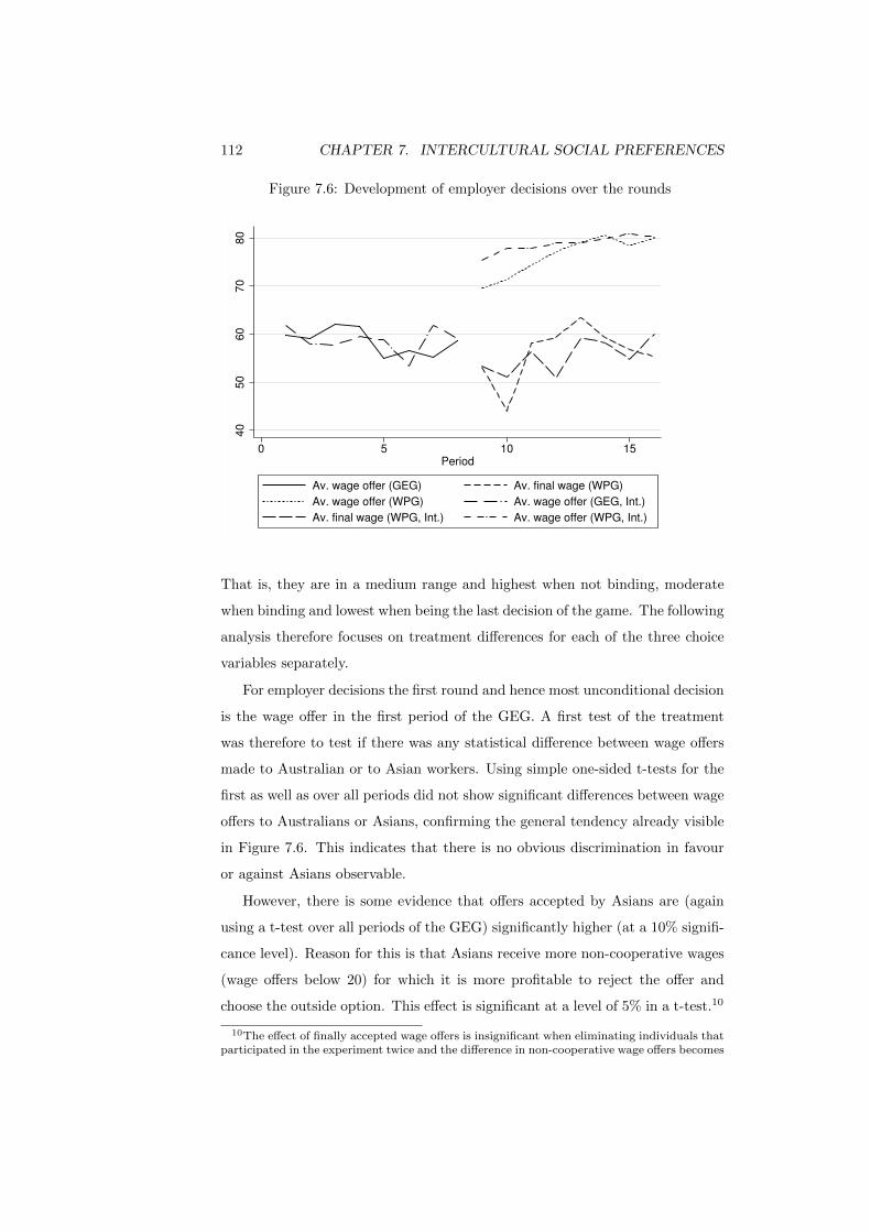
112 CHAPTER 7. INTERCULTURAL SOCIAL PREFERENCES
Figure 7.6: Development of employer decisions over the rounds
40
50
60
70
80
0 5 10 15Period
Av. wage offer (GEG) Av. final wage (WPG)
Av. wage offer (WPG) Av. wage offer (GEG, Int.)
Av. final wage (WPG, Int.) Av. wage offer (WPG, Int.)
That is, they are in a medium range and highest when not binding, moderate
when binding and lowest when being the last decision of the game. The following
analysis therefore focuses on treatment differences for each of the three choice
variables separately.
For employer decisions the first round and hence most unconditional decision
is the wage offer in the first period of the GEG. A first test of the treatment
was therefore to test if there was any statistical difference between wage offers
made to Australian or to Asian workers. Using simple one-sided t-tests for the
first as well as over all periods did not show significant differences between wage
offers to Australians or Asians, confirming the general tendency already visible
in Figure 7.6. This indicates that there is no obvious discrimination in favour
or against Asians observable.
However, there is some evidence that offers accepted by Asians are (again
using a t-test over all periods of the GEG) significantly higher (at a 10% signifi-
cance level). Reason for this is that Asians receive more non-cooperative wages
(wage offers below 20) for which it is more profitable to reject the offer and
choose the outside option. This effect is significant at a level of 5% in a t-test.10
10The effect of finally accepted wage offers is insignificant when eliminating individuals thatparticipated in the experiment twice and the difference in non-cooperative wage offers becomes

7.5. EXPERIMENTAL DECISIONS 113
These results are also confirmed in a Probit regression which shows a significant
effect indicating that wage offers accepted by Asians are higher; however, the
marginal effect of this estimation at the mean is not significant. The observation
that more non-cooperative wage offers are made to Asians might indicate that
some unwillingness to interact with Asians exists, but that wages above the non-
cooperative level are higher when made to Asians. However, the t-tests cannot
take account of potential game dynamics or individual-fixed effects, which will
be considered in the analysis below.
In the WPG employers have two decision variables, wage offers and final
wages. Simple t-test showed no significant differences for the first and over all
periods between the treatments. However, contrary to results of the GEG, there
were significantly less non-cooperative wage offers made to Asians. This effect
was statistically significant at the 1% level. When interpreting this result one
might want to recall the strategic importance of the wage offer in the WPG: It is
just cheap talk. However, if wage offers are perceived as promises by the employ-
ers, deviating from the promise might incur some psychological cost. If workers
know this, they will interpret wage offers as meaningful and higher wage offers
might increase worker effort. Employers might anticipate this, know they might
feel guilty when cutting down on promises and hence make lower offers due to
guilt aversion. Hence, if the wage offer takes a different role between the groups
(for example, to Asians it is just cheap talk while to Australians at least a rough
promise or indication) or if the level of feeling guilty differs depending on the
counterpart, higher wage offers to Asians may make sense. This interpretation
is further supported by the fact that Asians receive more non-cooperative wages
ex post (they are ripped off ; when being ripped off workers should have rejected
the offer and taken the outside option). This effect of non-cooperative ex post
wages is significant at the 10% level over all periods of the WPG.11 The result
of this significant difference is confirmed in a Probit regression which shows a
significant difference, but has an insignificant marginal effect at the mean.
Again, however, the results from the t-tests have to be interpreted with
care, as decisions might be dependent on other choice variables. This is most
obvious for final wage decisions in the WPG. Figures 7.7 and 7.8 illustrate the
significant at the 1% level.11When eliminating the double participants the significance level increases to the 5% level.

114 CHAPTER 7. INTERCULTURAL SOCIAL PREFERENCES
Figure 7.7: Relationship between final wages and received efforts
020
40
60
80
Fin
al w
age
0 2 4 6 8 10Effort
Australian group Intercultural group
potential connection between final wages and received efforts as well as wage
offers (promises). The following analysis therefore tries to take account of these
patterns, using (OLS) regressions on samples split between the two treatments
and joint regression with treatment and interaction terms.
Figure 7.8: Relationship between final wages and wage promises
45º020
40
60
80
Fin
al w
age
0 20 40 60 80 100Wage offer
Australian group Intercultural group
Wage offers are the first decision variable in each round of the GEG and
hence unconditional in a game-theoretic sense; however, decisions might still
depend on the history of the game. For example, if an employer expected to
receive a certain effort for a wage offered, after observing the effort chosen by the

7.5. EXPERIMENTAL DECISIONS 115
worker, expectations and hence optimal decisions might be updated although the
employer will not interact with the same worker in the next period. Such logic is
supported by regression results 1-4 in Table 7.7 which shows that efforts received
in previous periods lead to significantly higher wage offers and influence decisions
in an economically relevant way. A can be seen when comparing specifications 1
and 2, such an updating effect is stronger when employers interact with Asians.
Furthermore, Asians receive somewhat lower levels of wage offers, but, as can be
seen in the joint analysis in specifications 3 and 4 of Table 7.7, these effects are
not statistically significant and there is also no interactive effect with respect to
previous periods.
Table 7.7: Determinants of wage offers in the GEG
(1) (2) (3) (4)Split sample Joint sample
Australian Interculturalgroup group
Effortt−1 5.05*** 5.11*** 5.08*** 5.05***(0.52) (0.66) (0.43) (0.52)
Effortt−2 2.05*** 2.44*** 2.24*** 2.05***(0.65) (0.82) (0.52) (0.65)
Intercultural group -2.13 -3.55(2.63) (5.30)
(Effortt−1)*(Intercultural) 0.06(0.84)
(Effortt−2)*(Intercultural) 0.39(1.04)
constant 36.92*** 33.37*** 36.26*** 36.92***(3.68) (3.86) (2.90) (3.66)
N 240 216 456 456R2 0.38 0.41 0.39 0.39
The table shows potential determinants of wage offers in the GEG. Standard errors(clustered by individuals) are included in brackets. * indicates significance at the 10%level, ** at the 5% level and *** at the 1% level.
Similarly, wage offer decisions in the WPG are influenced by efforts received
in the previous period. The results as shown in Table 7.8 in specification 5 and 6
indicate that updating might be stronger when interacting with Australians, but
there is again no significant difference. Another potentially influential variable
in the WPG is the final wage paid in the previous period, which has a significant
effect on decisions and is very similar across treatments. Table 7.8 illustrates
this relationship, but specifications 7 and 8 again show that differences between
the treatments are not significant. Taken together, the results in Tables 7.7

116 CHAPTER 7. INTERCULTURAL SOCIAL PREFERENCES
and 7.8 document that positive reciprocity in the previous period increases the
willingness to be more kind in the current period. This statement is true for
wage offers in both games, across treatments and with no significant differences
between the treatments.
Table 7.8: Determinants of wage offers in the WPG
(5) (6) (7) (8)Split sample Joint sample
Australian Interculturalgroup group
Effortt−1 3.69*** 2.29** 3.12*** 3.64***(0.69) (1.02) (0.58) (0.68)
Final waget−1 0.12* 0.14* 0.12*** 0.13***(0.06) (0.07) (0.05) (0.05)
Intercultural group -0.24 7.76(2.93) (8.12)
(Effortt−1)*(Intercultural) -1.27(1.05)
constant 50.82*** 58.18*** 54.34*** 50.53***(6.33) (5.67) (4.71) (5.92)
N 258 239 497 497R2 0.32 0.24 0.28 0.29
The table shows potential determinants of wage offers in the WPG. Standard errors(clustered by individuals) are included in brackets. * indicates significance at the 10%level, ** at the 5% level and *** at the 1% level.
In a last step decisions over final in the WPG wages were analysed. Final
wages are decisions likely to be dependent on efforts received, but also poten-
tially on the promise made. Tables 7.9 and 7.10 illustrate the analysis investi-
gating this pattern and potential behavioural differences in interaction between
the groups. As can be seen in the split sample analysis of Table 7.9, the reaction
to the effort received appears to be higher when interacting with Asians. Fur-
thermore, the relationship to the wage offer is insignificant within both groups,
while the coefficient when interacting with Asians is noticeably lower. As both
split sample regressions have a relatively small number of observations and as
an influence of the wage offer makes sense when allowing for the wish to keep
promises, the variable was included and further investigated more detailed in
the joint sample analysis.
As can be seen considering the joint sample in specifications 11 and 12 of
Table 7.9, no lump-sum difference between the treatments can be determined.
However, this picture changes when allowing for interaction between the treat-
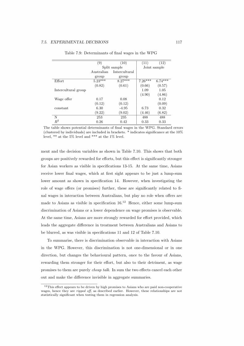
7.5. EXPERIMENTAL DECISIONS 117
Table 7.9: Determinants of final wages in the WPG
(9) (10) (11) (12)Split sample Joint sample
Australian Interculturalgroup group
Effort 5.23*** 8.27*** 7.26*** 6.74***(0.82) (0.61) (0.66) (0.57)
Intercultural group 1.09 1.05(4.90) (4.86)
Wage offer 0.17 0.08 0.12(0.12) (0.12) (0.09)
constant 6.30 -4.95 6.73 0.32(9.22) (9.02) (4.46) (6.82)
N 253 235 488 488R2 0.26 0.42 0.33 0.33
The table shows potential determinants of final wages in the WPG. Standard errors(clustered by individuals) are included in brackets. * indicates significance at the 10%level, ** at the 5% level and *** at the 1% level.
ment and the decision variables as shown in Table 7.10. This shows that both
groups are positively rewarded for efforts, but this effect is significantly stronger
for Asian workers as visible in specifications 13-15. At the same time, Asians
receive lower final wages, which at first sight appears to be just a lump-sum
lower amount as shown in specification 14. However, when investigating the
role of wage offers (or promises) further, these are significantly related to fi-
nal wages in interaction between Australians, but play no role when offers are
made to Asians as visible in specification 16.12 Hence, either some lump-sum
discrimination of Asians or a lower dependence on wage promises is observable.
At the same time, Asians are more strongly rewarded for effort provided, which
leads the aggregate difference in treatment between Australians and Asians to
be blurred, as was visible in specifications 11 and 12 of Table 7.10.
To summarise, there is discrimination observable in interaction with Asians
in the WPG. However, this discrimination is not one-dimensional or in one
direction, but changes the behavioural pattern, once to the favour of Asians,
rewarding them stronger for their effort, but also to their detriment, as wage
promises to them are purely cheap talk. In sum the two effects cancel each other
out and make the difference invisible in aggregate summaries.
12This effect appears to be driven by high promises to Asians who are paid non-cooperativewages, hence they are ripped off, as described earlier. However, these relationships are notstatistically significant when testing them in regression analysis.

118 CHAPTER 7. INTERCULTURAL SOCIAL PREFERENCES
Table 7.10: Determinants of final wages in the WPG
(13) (14) (15) (16)Joint sample
Effort 6.04*** 5.42*** 5.23*** 5.32***(0.97) (0.87) (0.82) (0.78)
(Effort)*(Intercultural) 2.52** 2.63** 3.04*** 2.92***(1.26) (1.25) (1.02) (0.96)
Intercultural group -15.70** -16.42** -11.25(6.93) (6.96) (12.82)
Wage offer 0.13 0.17 0.22**(0.09) (0.12) (0.09)
(Wage offer)*(Intercultural) -0.10 -0.22**(0.17) (0.09)
constant 15.00*** 8.30 6.30 1.57(5.64) (7.84) (9.17) (6.40)
N 488 488 488 488R2 0.34 0.34 0.34 0.34
The table shows potential determinants of final wages in the WPG. Standard errors(clustered by individuals) are included in brackets. * indicates significance at the 10%level, ** at the 5% level and *** at the 1% level.
7.5.2 Worker decisions
The analysis of worker behaviour is based on studying the acceptance of wage
offers and efforts. As for employer decisions, in a first instance simple one-sided
t-tests were used to analyse potential differences in the behaviour of Australian
and Asian workers. A worker’s first decision in both games is to accept or reject
the wage offer. There was no significant difference in acceptance behaviour
between Australians and Asians in both games. The major factor to reject an
offer is if this offer is non-cooperative. Furthermore, there is some tendency in
the WPG to reject offers if a non-cooperative wage was paid in the previous
period and this tendency is somewhat stronger for Asians. However, as these
relationships are not significant, they are not further investigated separately in
the following. Instead, rejections of offers are dealt with by recording worker
effort as zero.
The main decision variable of workers is hence their level of effort. Com-
paring effort levels between the two groups for the GEG showed that Asian
workers provided slightly more effort than Australian workers. This effect was
significant at the 10% level using a t-test over all periods and significant at a 1%
level when only taking efforts in response to cooperative wage offers (of 20 or

7.5. EXPERIMENTAL DECISIONS 119
above) into account. In the WPG, in contrast, there is no significant difference
between the groups. Figure 7.9 illustrates the development of efforts for the two
types of workers over the course of the experiment.
Figure 7.9: Development of effort over the rounds
34
56
7
0 5 10 15Period
Av. effort (GEG) Av. effort (WPG)
Av. effort (GEG, Int.) Av. effort (WPG, Int.)
Again, however, potential reaction patterns have to be taken into account,
as efforts are always conditional decisions. Most obviously, they are dependent
on wage offers.13 Figures 7.10 and 7.11 illustrate this conditional relationship
for both games, separated by treatment. The following analysis takes account
of these potential reciprocal relationships using regression analysis.
The results from the (OLS) regressions are included in Table 7.11. The
results from specifications 17-20 show that both Australians and Asians react
to wage offers in a very similar way. Furthermore, although there is a general
tendency of Asians to return higher efforts to employers, neither the level of
this nor the reaction pattern is significantly different from that of Australians;
hence, both groups behave similarly in the GEG.
As can be seen in Tables 7.12 and 7.13 the effort decisions in the WPG are
very similar to those observable in the GEG, despite the fact that wage offers are
not binding in the WPG. From the worker perspective wage offers are perceived
as meaningful signals, although the analysis of employer decisions showed that
13Evidently, effort decisions are also conditional on worker acceptance in the same stage. Ina further investigation it was analysed if some selection through the acceptance mechanismis apparent. However, as such a sub-sample-selection did not appear to play a role, only thesimplified results are described in the following.

120 CHAPTER 7. INTERCULTURAL SOCIAL PREFERENCES
Figure 7.10: Relationship between efforts and wage offers in the GEG
02
46
8E
ffort
0 20 40 60 80 100Wage offer
Australian group Intercultural group
Figure 7.11: Relationship between efforts and wage offers in the WPG
02
46
8E
ffort
0 20 40 60 80 100Wage offer
Australians Asians
offers did not play a significant role for final wages in employer decisions when
made to Asian workers and the effect was relatively weak in interaction between
Australians. Despite this observation it can be seen in specifications 25-28 of
Table 7.13 that there is no significant difference in worker decisions in response
to wage offers between Australians and Asians in the WPG .
In the WPG, however, efforts are not the last decision variable in each round,
but followed by the final wage decision. Due to this workers can get ripped off

7.5. EXPERIMENTAL DECISIONS 121
Table 7.11: Determinants of efforts in the GEG
(17) (18) (19) (20)Split sample Joint sample
Australian Interculturalgroup group
Wage offer 0.07*** 0.08*** 0.07*** 0.07***(0.01) (0.01) (0.00) (0.01)
Intercultural group 0.35 -0.27(0.32) (0.32)
(Wage offer)*(Intercultural) 0.01(0.01)
constant -0.84*** -1.11*** -1.15*** -0.84***(0.23) (0.22) (0.20) (0.23)
N 320 288 608 608R2 0.41 0.56 0.48 0.49
The table shows potential determinants of effort in the GEG. Standard errors (clus-tered by individuals) are included in brackets. * indicates significance at the 10%level, ** at the 5% level and *** at the 1% level.
Table 7.12: Determinants of efforts in the WPG separated by treatments
(21) (22) (23) (24)Split sample
Australian Intercultural Australian Interculturalgroup group group group
Wage offer 0.08*** 0.08*** 0.08*** 0.07***(0.01) (0.01) (0.01) (0.01)
Ripped offt−1 -0.22 -1.70**(0.61) (0.65)
constant -0.66 -0.66 -0.63 -0.25(0.48) (1.00) (0.48) (1.02)
N 320 288 320 288R2 0.33 0.21 0.33 0.25
The table shows potential determinants of effort in the WPG. Standard errors (clus-tered by individuals) are included in brackets. * indicates significance at the 10%level, ** at the 5% level and *** at the 1% level.
when they receive final wages.14 As can be seen in the Tables 7.12 and 7.13,
Asian workers reacted more strongly to these low final wages in the previous
period. This effect is significant at the 10% level, indicating that Asians (who
were generally ripped off more often) were more reactive to such behaviour.15
14As before, workers are ripped off when receiving final wages below 20.15An alternative control variable instead of being ripped off could simply be the final wage
received in the previous period. Indeed, using this variable, the effects described for the rippedoff variable appear to be even stronger. However, the final wage is significantly related tothe effort in the previous period, which is related to the effort in the current period throughindividual-specific effects. This in turn might overstate the role of the previous final wagereceived in the regression result. In contrast, whether an individual was ripped off in a period

122 CHAPTER 7. INTERCULTURAL SOCIAL PREFERENCES
As shown in Table 7.13, the difference in reactions to being ripped off can also
be seen in the joint-sample analysis. That is, workers react negatively to being
ripped off and this effect is driven by the behaviour of Asian workers, who show
a significant (and economically strong) reaction to it, while Australian workers
only show an insignificant tendency to react to this experienced counterpart
behaviour. However, despite this slight difference in reactions to being ripped off,
reaction patterns are generally very similar across the two groups as otherwise
there does not seem to be a significant lump-sum difference or a different reaction
to the wage promise depending on whether the worker is Australian or Asian.
Or, in other words, the cultural identity does not seem to play a major role in
worker decisions or decision patterns.
Table 7.13: Determinants of efforts in the WPG including both treatments
(25) (26) (27) (28)Joint sample
Wage offer 0.08*** 0.08*** 0.08*** 0.08***(0.01) (0.01) (0.01) (0.01)
Intercultural group -0.22 0.00 -0.17 0.07(0.47) (1.10) (0.46) (0.47)
(Wage offer)*(Intercultural) -0.00(0.01)
Ripped offt−1 -1.01** -0.21(0.46) (0.61)
(Ripped offt−1)*(Intercultural) -1.48*(0.88)
constant -0.58 -0.66 -0.43 -0.52(0.48) (0.48) (0.49) (0.48)
N 608 608 608 608R2 0.27 0.27 0.29 0.29
The table shows potential determinants of effort in the WPG. Standard errors (clus-tered by individuals) are included in brackets. * indicates significance at the 10%level, ** at the 5% level and *** at the 1% level.
7.6 Conclusion
The original question in the design of the experiment was to investigate if Aus-
tralians would discriminate against Asians and if Asians would decide differently
from Australians in an experimental labour market. Additionally, two differ-
ent games were used to investigate if the framework of interaction between the
was not significantly related to the previous period’s effort. Therefore, the ripped off variableis chosen here as a more conservative approach.
7.6. CONCLUSION 123
cultures would change discriminative behaviour. Furthermore, experimental
decisions were combined with observational data from a questionnaire, which
included numerous trusting variables; trust was investigated as it is theoretically
seen to differ between a Western (Australian) and an Eastern (Asian) culture
and to play an influential role for decisions in the experimental labour market
game used in this study. Given questionnaire and experimental results, the orig-
inal questions can be answered as follows: Analysis of general trusting attitudes
showed that on a combined trusting scale there was no significant difference
between Australians and Asians. This would indicate that Asians migrating to
Australia might not be representative of their home country peers or adapt to
Australian values and attitudes relatively quickly. However, the picture is more
nuanced, as the two groups significantly differ in different domains of trusting
attitudes.
However, how decision-relevant were these attitudes in the experiment? The
data showed that any differences in trusting attitudes did not drive behavioural
differences between Australian and Asian workers.16 The statistical and eco-
nomic significance of all singular trusting attitudes on decisions was relatively
low for any trust-dependent experimental decision variable (hence wage offers
in the GEG and efforts in the WPG) and a relationship was virtually non-
existent for the combined trusting attitude. As decision patterns of Australian
and Asian workers were very similar, the results suggest comparability between
the two cultural groups.
Furthermore, experimental results also indicated that the interaction be-
tween the two groups was similar in Australian and intercultural Australian-
Asian sessions: There were no major level differences in outcomes between the
groups once controlling for reciprocal patterns between employers and workers.
There was, however, a difference in interaction when Australian employers inter-
acted with Asian workers (as opposed to Australian workers) in the WPG. That
is, while worker effort was rewarded similarly for both types of workers in the
GEG, it was more strongly reciprocated in the WPG when Asians were in the
worker role. This would indicate that reverse discrimination towards Asians is
observable as they are treated more kind. At the same time there was, however,
16That is, the trusting attitudes in which Australians and Asians differed significantly didnot lead to strong changes in decisions.

124 CHAPTER 7. INTERCULTURAL SOCIAL PREFERENCES
either (a) a lump-sum lower base payment to Asian workers who hence had to
start at a lower general reciprocity level. When looking even more specifically,
though, (b) the results rather indicated a different role of the wage promise to
workers. This offer was meaningful when made to Australians, but basically
pure cheap talk when made to Asians. As both groups of Asian and Australian
workers reacted very similarly to these wage promises, treating them as mean-
ingful, this indicates discrimination towards Asians. Hence, the experimental
game mattered for the interaction between Australians and Asians.
Finally, one might also want to interpret the results of the study included in
this chapter in terms of their policy relevance, as this was a driving factor moti-
vating the research question of investigating the interaction of Australians and
Asians. Hence, it is possible to read the results in a light of Asian migration to
Australia and its impact on the labour market. As such this study complements
and adds more nuance to the study by Guillen and Ji (2011). The first central
result and observation of the data was the relative similarity of the groups in
terms of their attitudes as well as their behaviour. In the general migration con-
text this would indicate that an integration into the Australian labour market
should be unproblematic. However, there might be drawbacks when employer-
worker interaction relies on softer factors that facilitate reciprocal interaction in
the workplace. This would follow from the second central observation indicat-
ing that wage promises to Asians are cheap talk, but perceived as meaningful
and that being ripped off has a particularly negative impact in interaction with
Asians. Put differently, immigrants might expect that soft factors like promises
have the same meaning in interaction with them as with locals, but the local
group might not value them equally when dealing with migrants. Finally, the
third observation was that Asians were rewarded more than Australians for their
effort in the promising-framework. Hence, direct rewards might even work bet-
ter in the intercultural context. All three of these observations are factors which
should be taken into account on a management level in companies with many
migrant workers, as well as when designing workplace or immigration policies.
Finally, despite the fact that the results of the study are interesting and
contain information valuable for policy-makers and managers, the study has
also its limits: For example, it looked at a very specific subject population and
7.6. CONCLUSION 125
the students in the employer role are not likely to be employers of migrants
tomorrow. Also the external validity of a laboratory-based study like this one
is always limited. However, the study used a subject pool likely to be affected
by the interaction studied and results from laboratory studies are often not too
far from reality, leaving an overall positive conclusion about the usability of the
results.

126 CHAPTER 7. INTERCULTURAL SOCIAL PREFERENCES

Chapter 8
The role of policy in
shaping social preferences1
8.1 Introduction
The importance of labour market discrimination for economic outcomes has
been and continues to be an intensely debated topic in the academic literature.
Discrimination, that is, a change in behaviour towards groups of people with
certain characteristics, exists in basically all societies. Some attributes that are
a basis for discrimination are relatively obvious or at least have a natural foun-
dation, such as gender or height, others are more arbitrary. When reasons for
discrimination are arbitrary, it is rarely obvious what motivates discrimination
on a behavioural level. This is particularly critical for understanding taste-
based elements of discrimination (as introduced by Becker, 1971), in contrast
to statistical discrimination.
While it is easy to think of a taste as intrinsic and exogenous evolving on a
purely individual level, public policies and official institutions are also candidates
for establishing discrimination based on tastes; for example, they could not only
help to identify suitable cut-offs for statistical comparisons like a job certification
or an academic degree, but could also give rise to artificial tastes. The study
1This chapter is based on collaborative work with Uwe Dulleck and Yumei He (see alsoDulleck et al., 2012a).
127

128 CHAPTER 8. POLICY-INDUCED SOCIAL PREFERENCES
described in this chapter investigates this impact of policies on individual-level
discrimination in the labour market using a real, policy-induced attribute, the
Chinese hukou status. The hukou system institutionally segregates the labour
force into two types, locals and migrants. In Chinese cities, being classified as a
migrant deprives individuals of institutional “benefits”, i.e. (mainly) access to
public housing, employment and education. The experiment described in this
chapter studies how the presence of this system influences individually motivated
taste-based discrimination in an environment where different status is assigned
to seemingly identical individuals.
The experimental framework used here for studying discrimination based on
the hukou status allows to identify discrimination based on tastes and based
on statistical beliefs. Despite being independent by construction, in reality
taste-based and statistical discrimination can interplay through psychological
dynamics; for example, receiving low wage offers that are perceived as unfair
can cause disadvantaged workers to shirk, leading to a dual labour market where
high and low reciprocity employer-worker equilibria are present (as could be
reflected in the model by Akerlof and Yellen, 1990).
The notions of taste-based and statistical discrimination can, however, be
blurry, as both are usually used for analysing aggregate phenomena that em-
ploy behavioural foundations within individuals only as vehicles to ensure that
equilibrium outcomes can be derived theoretically. Therefore, a slight redef-
inition of the terms describing discrimination is used for the study presented
here: Throughout this chapter, the taste to discriminate against migrants is
referred to as an individual’s preferences which cannot be explained by ob-
jective or subjective beliefs or expectations about the behaviour of migrants.
Or, in terms of the framework of thinking used throughout this thesis using
Uij(Xi, Xj) = αiXi + βijXj as an illustration for social preferences, the dif-
ference between statistical and taste-based discrimination could be understood
such that the discrimination parameter ∆β = βlocal − βmigrant would be con-
stant for taste-based discrimination even when information about the counter-
part becomes available, while being information-dependent for statistical dis-
crimination.
Furthermore, given the reciprocal character of interaction in a gift exchange

8.1. INTRODUCTION 129
framework, it might be more reasonable to shade own offers for individuals mo-
tivated by taste-based discrimination, but not so for statistical discriminators.
Notably, this definition of taste-based discrimination is wider than the common
one, which describes it as a dislike to interact with another social group and
models it as a (psychic) cost when reciprocally interacting with this other group.
While the definition used here could entail psychic costs, it could also include
perceived differences of what is a fair split between the groups. In contrast,
statistical discrimination could be based on (potentially incorrect) beliefs, but
disappears with full information and in the absence of unobservables. Indeed,
the discrimination investigated in this study does not primarily address the dis-
crimination in hiring behaviour, but in a sense the after-market discrimination
in terms of reciprocity between employers and workers. Given the importance
of behavioural interaction in generating mutual benefit, discrimination in these
realms might be of equally high (if not often higher) importance. Given the
latency of such behavioural phenomena, using experiments is one potential and
even obvious tool to unveil such unobservable effects.
To study the discrimination of migrants, for the study presented here house-
hold aids were hired on their normal labour market in Nanjing for an artefactual
field experiment (see Harrison and List, 2004, for a classification). Discrimina-
tion was captured by controlling for hukou status, which is unchangeable and
exogenous for the participants of the experiment, by matching either groups of
all locals and all migrants to the roles of employers and workers. As described
in the introduction to this part, a gift exchange game (GEG) and the wage
promising game (WPG) were used. The conjunction of the GEG and the WPG
allows to disentangle statistical from taste-based discrimination: In the WPG
employers first make a non-binding wage offers; the worker observes this offer
and chooses her effort level; finally, the employer observes the effort choice and
chooses the final wage she wants to pay. Thus, in the WPG lower effort cannot
explain lower wages paid to migrants as wages are not based on beliefs.
Results of the experiment show that discrimination based on hukou status is
observable when wage offers are binding. Discrimination further increases when
non-binding promises can be made as migrants get promised similar wages, but
get paid significantly less in their final wages for the same effort provided. In
130 CHAPTER 8. POLICY-INDUCED SOCIAL PREFERENCES
contrast to the finding that the status of the counterpart motivates discrimina-
tion, own status does not lead to differing decisions (e.g. based on an underdog
identity, see Akerlof and Kranton, 2000), indicating that it is rather taste-based
than statistical discrimination that is observed. Hence, official segregation based
on hukou status is not a reflection of statistical characteristics, but a motivator
of taste-based discrimination. This observation is true although hukou status for
the experimental subjects, who are otherwise homogeneous, is an exogenously
imposed characteristic and the socio-economic group studied in this experiment
is effectively unable to change their status.
With its focus on the difference between taste-based and statistical discrim-
ination the approach in this chapter is closest to the study by Fershtman and
Gneezy (2001) who show how stereotypes between students with different fam-
ily history (Ashkenazic and Eastern Jews) can motivate discrimination using
trust and dictator games, finding that discrimination is statistical, but based
on stereotype-induced, incorrect (and self-denied) beliefs. While Fershtman and
Gneezy are studying arbitrary discrimination based on family history, the in-
terest here is particularly in the role of public policy, or official institutions
that motivate discrimination.2 In the framework studied here the state has at-
tributed hukou status exogenously to the subjects used for the study almost as
in a laboratory setting, like studied by Ball et al. (2001) who artificially induce
status to laboratory participants.3 They find that lower status participants be-
come more submissive in interaction. While similarly being interested in the
emergence of motivations to discriminate, the study included in this chapter
differs from their approach when making use of a real public policy for the ex-
perimental treatment and by studying subjects from a normal labour market for
whom hukou status is exogenous and unchangeable, making them a particularly
well-suited subject pool.4 By this it is possible to study how a real institution
2Additionally, in this study repeated and direct interaction is observed, giving rise toreasons for shading offers made in decisions by employing the choice method instead of thestrategy method. By this, the experiment described in this chapter also gathered informationfor the additional result that learning does not reduce discrimination.
3Ball et al. give participants a performance task and then assign status; however, statusis independent of performance in the task.
4Using non-student subjects in experiments is not completely uncommon in the literature(e.g. Gachter and Herrmann, 2010), but studying individuals in their naturally occurringenvironment and in field experiments is still relatively new (but see List, 2006a; Marechal andThoni, 2007).

8.2. SEGREGATION BASED ON THE HUKOU SYSTEM 131
leads to changes in motivations for discrimination and to disentangle statistical
from taste-based discrimination by introducing the WPG.
Furthermore, the study included here can add to the understanding of the
hukou system and its social consequences as described by Wang and Zuo (1999)
and investigated more quantitatively in the subsequent literature, mainly using
survey data (e.g. Demurger et al. 2009). This highly policy-relevant topic
is addressed by employing an experiment that eliminates factors difficult to
measure in surveys.
8.2 Segregation based on the hukou system
China’s hukou or household registration system requires people to live and work
only where they have official permission to do so. It was officially introduced
in 1958 to regulate migration, particularly between rural and urban regions.
Every citizen is to be registered as either agricultural (rural) or non-agricultural
(urban) and hukou status is passed on from parents to their children. This
classification leads to a separation within the city between locals (urban hukou
individuals registered in the region of their work place) and migrants (individuals
from an agricultural area, or another urban area). For almost two decades,
holders of rural hukou were barred from working in urban areas. Since the
beginning of economic reforms in the late 1970s, small numbers of rural migrants
were allowed to enter the cities. As China’s export and service industries began
to grow rapidly in the 1980s and 1990s, increasing numbers of rural workers
have been permitted to migrate to the cities to meet the demand for cheap
labour. However, while migrants are allowed to work in the cities, their rural
hukou status does not allow them access to many benefits that automatically
accrue to urban hukou holders.
Originally hukou status was derived from birth place and was not negotiable
(with very few exceptions). However, since the mid-1990s, this rigidity has been
relaxed and some local governments can now grant urban hukou to holders of
rural hukou who own stipulated levels of real estate or assets in the cities.
Sometimes hukou status is also adapted as rural districts or land are integrated
into an expanding city surface; in these cases people can be compensated for the

132 CHAPTER 8. POLICY-INDUCED SOCIAL PREFERENCES
loss of land through a change in their hukou status. Despite such relaxation,
the dualistic structure has generally remained intact. In practice very few rural
migrant workers are wealthy enough to take advantage of this policy change
and the effects of geographical incorporation are globally small. While the
hukou system has continued to be dynamic, segregation based on this invariable
status is still relevant for most (low income and low education rural) migrants,
especially in economically attractive metropolitan areas.
Due to its social and economic consequences - particularly being cut off from
public education, housing and employment, changing the hukou system has been
in the political discussion as well as a topic of the economic literature. Wang
and Zuo (1999) outline the rather precarious conditions that urban migrants
live in, describing the situation of migrants such that “[m]ost rural migrants
arrive in cities to take up marginal jobs that are characterised by long hours,
poor working conditions, low and unstable pay, and no benefits - jobs which
are unattractive to urban residents”(p.277). Wang and Zuo (1999) point out
that migrants often work longer hours and work for lower pay - indicating that
status and discrimination lead to changes in migrants’ behaviour, which could
blur statistics of income discrepancies between the social groups and make them
appear more benign.
The literature has evaluated various aspects of the hukou system and has
tried to get a clearer picture of its consequences. Liu (2005) quantifies and
estimates the value of urban hukou to rural individuals and concludes that it
would range between 2,741 Yuan to 45,654 Yuan,5 based on accessibility of
quality education, better-remunerated jobs and a better quality of life. The
major channel for differences is the attainability and price of education, which
illustrates that the hukou system leads to a persistence of social inequalities,
a result also reported in a simulation approach by Whalley and Zhang (2007)
who compare the status quo with a hypothetical situation without hukou-based
mobility restrictions.
Focusing on labour market outcomes, Lu and Song (2006) look at survey data
and observe that working conditions are to the detriment of migrants. While
they find no significant differences in total wages based on hukou status, differ-
5At a fixed exchange rate of 0.1207 at the time this research was published this reflectedvalues of USD 330 and 5,510 (between 22% and 55% of per capita GDP).

8.3. EXPERIMENTAL IMPLEMENTATION AND PARTICIPANTS 133
ences channel mainly through fringe benefits that are unavailable to migrants.
They also restate that migrants work for lower pay and longer hours, and that
the vast majority is employed on short-term contracts. Similarly, Demurger
et al. (2009) show that unstable working conditions are prevalent among mi-
grants and that significant differences in hourly wages exist. Limited access to
certain jobs due to hukou status restrictions, hence discrimination, is a main
contributor to these differences.
Zhang (2010) makes the same point that institutional discrimination based
on hukou status reduces the number of jobs available to migrants, increases their
job search costs and the cost of losing jobs. Based on search cost arguments,
migrants stay in jobs longer than their counterparts with local hukou status.
Hence, migrants remain in jobs with less desirable working conditions and wages,
implying that status affects behaviour. However, it is less clear how status
also leads to changes in motivations (or preferences) for discrimination on an
individual level.
8.3 Experimental implementation and partici-
pants
8.3.1 Experimental implementation
As described in the introduction to this part, the GEG and the WPG were used
to look at potential differences in behaviour of locals (i.e., those with local hukou
status) and migrants (i.e., those with hukou status from outside of the city).
The games were explained in a labour market framing and in very simple and
labour market specific language. The GEG was used as the study was interested
in the labour market effects of the hukou system. The WPG was added as it
captures labour markets where workers are less protected, in particular where
it is hard to ensure that wages are paid. It also allows to differentiate between
statistical and taste-based discrimination when comparing the results to those
from the GEG as in the WPG: Employers know the effort of the worker before
deciding about the wage; that is, wages are not based on the workers expected
effort (or trustworthiness, which the results in the GEG informed about).

134 CHAPTER 8. POLICY-INDUCED SOCIAL PREFERENCES
Each game was played for 8 consecutive rounds. The order of the games was
changed between sessions. Participants received instructions for each game just
before the first round of this game (i.e., before rounds 1 and 9, respectively).
They were assigned their role as either a worker or an employer at the beginning
of the experiment and remained in this role for all rounds. Sessions were organ-
ised controlling for hukou status of participants and groups were matched such
that there were groups of 8 participants (= 1 session) which purely consisted of
locals, groups that purely consisted of migrants, groups in which the employer
role was always taken by a local and the role of the worker was always taken by
a migrant as well as the reverse. Table 8.1 shows the number of participants in
each constellation used in the experiment.6
Table 8.1: Participants by constellation
EmployerLocal Migrant
WorkerLocal 80 (48,32) 24 (24,0)
Migrant 96 (56,40) 80 (32,48)
The table shows the number of participants for each constellation. The num-
bers in brackets indicate for how many of these participants the GEG or WPG
were played first, respectively.
In case the two hukou groups interacted, the status of the counterpart was
explicitly communicated to participants on their computer screens. The instruc-
tions screen included a phrase saying that in the current session the role of the
employer was always assigned to a person with local hukou and the role of the
worker was always assigned to a person with migrant hukou, or the correspond-
ing reverse. While this information was included on the screen, it was not read
out to participants together with the other descriptions, which the participants
were asked to read along. The reason for this was to avoid experimenter de-
mand effects greater than what would be observable in a real-life situation.7
6The small number of participants in the constellation migrant employer - local workerresulted from the elimination of 16 participants due to a mistake in seating them. Moreparticipants of the required type were not available at the time, therefore these sessions werenot rerun. Furthermore, the game reversal was not played in this constellation, as alreadyplenty of information had been collected on the game order effect. Finally, the number ofobservations was reduced in this particular matching (and not in others), as it appeared tobe the one with the least policy relevance.
7Hukou status is often not directly observable, but can easily be looked for on a person’sidentity card. Similarly, information about status was provided, but it was not directly pointedto, although participants knew that their status was previously checked and they were provided
8.3. EXPERIMENTAL IMPLEMENTATION AND PARTICIPANTS 135
The instructions to participants can be found in the appendix.
The experiment was conducted in a computer laboratory using z-tree (Fis-
chbacher, 2007). A computerised laboratory setting was chosen as it allowed
collecting data on interactions between participants in the two games relatively
easily and to observe whether patterns of interaction and discrimination changed
over periods. Using computers also facilitated employing the choice method,
which seems desirable in a setting investigating a potentially emotional decision
of discrimination.
The complete experiment lasted around 1.5 to 2 hours. Seating and in-
structing participants made up the largest part of this time.8 The conversion
rate from experimental to local currency was 5 experimental dollars = 1 Yuan.
Consequently, participants received between a minimum of 40 and up to 120,
averaging around 80 Yuan - or 40 Yuan per hour - for their participation in the
experiment. This compares to usual hourly pay between 15 to 20 Yuan.9
8.3.2 Experimental participants
For the study, household aids, so-called ayis, were recruited as experimental
participants from the city of Nanjing, a group that was particularly suitable
for the aim of this study. In Nanjing this occupation is pursued by both locals
and migrants, and the groups are comparable across hukou status; for example,
cultural differences (e.g. in cooking styles or dialects) are relatively small for
the sample used here. This, together with the fact that participants for this
study are from a low income group makes it possible to treat hukou status as
exogenous.
Participants were hired through their normal labour market channels and
based on usual hiring conditions for this type of workers. Some participants
with participant numbers based on their name. Hence, the treatment variable of whetherparticipants were matched with a migrant or a local counterpart was only introduced by onesentence on the computer screen.
8According to observations by the experimenters, these non-student participants did notneed much more time for making decisions than students that played the experiment do inthe weeks before in sessions organised to familiarise the local team of experimenters withconducting economic experiments. This local team of 6 students conducted the experimentalsessions. Furthermore, at least one of the authors was additionally present at each of thesessions.
9Higher than regular market level payments were necessary, as experiments were run onSundays, where opportunity costs were higher. Furthermore, participants incurred some extratravel cost (time and monetary) to the location of the experiment.
136 CHAPTER 8. POLICY-INDUCED SOCIAL PREFERENCES
were also recruited through a local trading school.10 More detail on ayis, their
labour market in Nanjing and the recruitment procedures is included in the
appendix.
The experimental sessions were run on 5 days with a total of 37 groups and
8 participants in each group. Sessions took place over the course of 7 weeks
in November and December of 2010. Due to the minimum requirements on
reading abilities and the necessity to use groups of 8 participants, 26 participants
(9%) were sent home after paying them a show-up fee. Due to a mistake in
matching participants, 2 groups had to be dropped from the sample, leaving
280 participants of which 99% were females. 2240 individual decisions were
collected for each of the two experimental games.
The original assumption of comparability across hukou status, which made
household aids suitable as experimental subjects, was corroborated using a
computer-based questionnaire at the end of our experiment. Although it was
not possible to ensure that every participant completed the questionnaire, most
participants answered most of the questions. Main summary statistics from the
questionnaire are included in Table 8.2.
The data confirms the conjecture about comparability. More particularly,
the average age of participants is in their early 40s. Average monthly income
just somewhat below 2 thousand Yuan, which shows that participants are in a
comparatively low income category. Hours worked are similar for both groups,
although migrants work slightly more for their higher income. However, com-
paring income and work hours indicates that hourly wages are comparable for
both groups. In contrast, however, differences in rents paid are noticeable de-
spite equal incomes; this confirms lines of research indicating that economic
differences based on hukou status are mainly channelled through fringe benefits
such as available housing and costs of education.
Most variables are similar across the groups and differences are as expected.
Migrants have more children, and have more brothers and sisters, reflecting
general demographic factors within the Chinese population.11 Migrants have
lived in Nanjing for a shorter time, but are not necessarily new arrivals; some
have lived there all their lives. Also, some locals have not lived in Nanjing all
10These individuals are identified with the variable “certificate”in later analysis.11For example, the enforcement of the one child policy is more strictly applied in the cities.
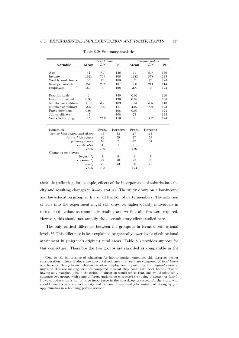
8.3. EXPERIMENTAL IMPLEMENTATION AND PARTICIPANTS 137
Table 8.2: Summary statistics
local hukou mirgant hukouVariable Mean SD N Mean SD N
Age 44 7.4 136 41 6.7 136Income 1911 703 108 1982 578 123Weekly work hours 35 23 108 37 26 124Rent per month 276 301 107 398 314 114Employers 3.7 2 108 3.8 2 124
Fraction male 0 140 0.02 140Fraction married 0.98 136 0.99 136Number of children 1.19 0.4 109 1.51 0.6 118Number of siblings 3.6 1.5 111 4.02 1.8 123Party members 0.04 108 0.05 124Job certificate 45 108 52 124Years in Nanjing 25 17.9 116 9 7.2 124
Education Freq. Percent Freq. Percentsenior high school and above 45 33 17 13
junior high school 80 59 77 57primary school 10 7 42 31
uneducated 1 1 0Total 136 136
Changing employersfrequently 7 6 9 7
occasionally 22 20 25 20rarely 79 73 90 72Total 108 124
their life (reflecting, for example, effects of the incorporation of suburbs into the
city and resulting changes in hukou status). The study draws on a low-income
and low-education group with a small fraction of party members. The selection
of ayis into the experiment might still draw on higher quality individuals in
terms of education, as some basic reading and writing abilities were required.
However, this should not amplify the discriminatory effect studied here.
The only critical difference between the groups is in terms of educational
levels.12 This difference is best explained by generally lower levels of educational
attainment in (migrant’s original) rural areas. Table 8.3 provides support for
this conjecture. Therefore the two groups are regarded as comparable in the
12Due to the importance of education for labour market outcomes this deserves deeperconsideration. There is also some anecdotal evidence that ayis are composed of local loserswho have lost their jobs and who have no other employment opportunity, and migrant winners,migrants that are making fortunes compared to what they could earn back home - despitehaving only marginal jobs in the cities. If education would reflect that, one would mistakenlycompare two groups with some different underlying characteristic (being a winner or loser).However, education is not of large importance in the housekeeping sector. Furthermore, whyshould winners migrate to the city and remain in marginal jobs instead of taking up jobopportunities in a booming private sector?

138 CHAPTER 8. POLICY-INDUCED SOCIAL PREFERENCES
sense that the level of education does not hint to deep-rooted (e.g. ability-based)
differences between the two groups.
Nevertheless, levels of education in the subject pool could change the oppor-
tunity costs of the participants outside of the laboratory. If anything, an ex-
perimental approach mediates this effect and makes decisions of the two groups
more comparable. Furthermore, a control variable on educational level was used
when testing the robustness of results in the analysis described below and no
strong effect (both statistically and economically) was apparent.13 The con-
clusion from this procedure of scrutinising the a priori assumption is that the
two groups are remarkably similar, making them suitable to be studied in an
experimental study that draws on the notion that hukou status can be treated
as an exogenous factor.
Table 8.3: General levels of education in urban and rural areas
Uneducated Primary Junior high Senior highschool school school or more
Rural 10% 38% 42% 9%Urban 3% 17% 35% 44%
Source: National Bureau of Statistics of China (2010)
8.4 Experimental results
8.4.1 Hypotheses
The experimental data was analysed to investigate if discrimination against the
migrant group is observable and to disentangle statistical discrimination, hence
treating the migrant group differently mainly because they react differently in
the experiment, from non-statistical discrimination, hence mainly taste-based
discrimination or, as migrant status is originating from an (arbitrary) official
institution, the exploitation of the lower social status of migrants. The expec-
tation given prior results from the literature was that discrimination would be
13The questionnaire also provided information about how often workers had to change theiremployers. It becomes obvious that employer turnover is generally not very frequent amongthe two groups. I.e., over 70% of the workers report that employer turnover is rare. Thisresult could indicate that job security is a major factor of importance in the housekeepingindustry. In fact, this could be a source of behavioural differences if the attainability of jobsecurity is different for locals and migrants, which probably cannot fully be captured by anyof the control variables used.
8.4. EXPERIMENTAL RESULTS 139
observable independent of whether the employer or the worker role is taken by
the migrant. However, it was less clear if this institutional discrimination of mi-
grants motivates individual-level, taste-based discrimination or if it goes along
with some statistical attributes of the migrants.
Nevertheless, one conjecture was that the mechanism for this is that official
discrimination helps to establish a social perception that migrants are an inferior
social group who can be treated worse and exploited more. This would be
reflected in results from the experimental games such that migrants get paid
lower wages although they do not fundamentally behave differently from locals.
Potentially they might even return more to their counterparts, as they are aware
of taste-based discrimination against them and are used to over-compensate for
this.
As for the results of the two games, the experimental design was aimed to
help identify what role statistical discrimination plays in decisions: Discrimina-
tion by employers in the gift exchange game could be partly driven by beliefs
that migrants will return more, while in the wage promising game the wage
decision is made ex post, meaning that statistical reasons cannot explain differ-
ences in discrimination. Assuming discrimination to be primarily taste-based,
discrimination of migrants was expected to be lower for wage promises in the
wage promising game and higher in the final wage decision compared to wage
offers in the gift exchange game.
Finally, if discrimination is mainly taste-based, one would expect that giving
less to migrants will be independent of the role taken in the experiment and that
migrants also receive less effort when they are in the employer role. Further-
more, if statistical discrimination does not play a significant role, own status
of employers and workers does not lead to significant differences in decisions
depending on whether the decision maker is a migrant or a local.
8.4.2 Experimental data
The analysis of the experimental data shows that discrimination of migrant
counterparts is observable and that it is different between the games; further-
more, hukou status of individuals has, if anything, only a weak effect on own
decisions. Together these results indicate that official discrimination based on

140 CHAPTER 8. POLICY-INDUCED SOCIAL PREFERENCES
hukou status leads to individual-level discrimination which is taste-based rather
than statistically motivated.
In order to come to these conclusions the experimental data was analysed
taking account of the structure of the data (the distribution of the decision
variables), the strategic nature of decision variables and the way treatments
were designed. For example, conditional and reciprocal relationships (higher
wage offers and wage promises are responded to by higher effort and higher
effort by higher final wages) can be expected; simple overviews of the decision
variables clearly confirm this conjecture.
As multiple periods of decisions in the games were used, time effects (earlier
and later periods) were checked as well as the individual decision histories of
participants. Furthermore, game order effects were controlled for (when the
wage promising game was played first, wage offers, effort levels and final wages
were approximately 10% higher). The main aspects are described below; more
detailed information is included in the appendix.
Structure of the decisions variables
In the gift exchange game a high proportion of wage offers in the high and
maximum category (w ≥ 70) can be found. These wage offers are reciprocated
by workers, leading to a large proportion of high efforts. Furthermore, there is
a second peak of efforts in the rejection and minimum-effort region which to a
large degree reflects low wage offers that cannot be responded with higher effort
levels without incurring a loss to the worker (compared to the outside option of
rejecting the offer). Some non-reciprocal (selfish payoff-maximizing) decisions
are also observable.
In the wage promising game decision variables and reciprocal patterns are
very similar to patterns in the gift exchange game. This indicates that the cheap
talk character of the wage offer does not play a big role for either employers nor
workers. Employers seem to be unwilling to break their promises and reciprocate
high efforts with high final wages. However, as final wages are conditional
on wage offers, the acceptance of the offer and on effort (both of which are
themselves conditional), they require careful interpretation.
Table 8.4 provides an overview of the decision variables in the two games.

8.4. EXPERIMENTAL RESULTS 141
They are separated by treatments and game order, as significant order effects
were found in the analysis. Reading from this overview table, discrimination
against migrants can be observed, although differences do not seem to be signif-
icant. That is, except for wage offers when the GEG was played first, transfers
(hence GEG wage offers, WPG final wages and efforts) were always lower when
the experimental counterpart was a migrant. However, it has to be taken into
account that not all decisions are unconditional and the following analysis in-
cludes more controls to account for these factors. This fact is also reflected by
the large variance around the decision variables.
Table 8.4: Summary statistics looking on the importance of the game order andthe status of experimental counterparts
GEG first WPG firstLocal Migrant Local Migrant
counterpart counterpart counterpart counterpartVariable Mean s.d. Mean s.d. Mean s.d. Mean s.d.
GEG
wage offer 68 31 72 26 79 27 74 26
effort 5.3 4.1 4.6 4.1 5.9 3.9 5.0 3.8
WPG
wage offer 70 31 72 25 83 25 76 24final wage 71 33 63 33 76 31 72 29
effort 5.9 4.0 4.8 3.8 6.6 3.6 5.4 3.8
Having identified the general structure, the experimental data was analysed
with respect to the hypotheses in more detail. Reflecting the nature of the
decision variables and structure of the data, employer and worker decisions were
investigated separately. In order to take account of the conditional nature of the
variables and to get a better picture about possible patterns and dynamics of
discrimination, (OLS) regression analyses were used. Functional specifications
were chosen reflecting the structure of the data as well as after considering
various alternatives.14 Both for employer and worker decisions specifications
that included the main control variables and further information from the post-
experimental questionnaire were considered. These included information on
14This included, for example structural models with a breakpoint at w=20, below whichworkers should reject offers.

142 CHAPTER 8. POLICY-INDUCED SOCIAL PREFERENCES
income, work hours, rental payments, employer turnover, education level, age,
marital status, gender and membership in the communist party.15 However, in
the final specification only such questionnaire variables were included that had
been significant in prior specifications and did not reduce the sample too much.
Including or excluding demographic controls did not significantly influence the
effect of the treatment variables.
For both employers and workers binary treatment variables of playing with
migrants and of being a migrant oneself were used (indicated by the variables
Migrant employer and Migrant worker). It was also checked whether using sepa-
rate variables for all of our four treatments was necessary, or if it was legitimate
to pool the data. There is no indication that a further variable, “Migrant em-
ployer and Migrant worker”, had a significant influence. This also indicates that
ingroup-outgroup effects do not drive results. Alternative regressions, as well
as a short discussion of this issue is included in the appendix. Furthermore, bi-
nary variables for the order of the games (GEG first) and for the days on which
the experiment was conducted were included, as these had been significant in
essentially all specifications. Results from two different specifications for both
employers and workers are reported in the analysis below: One including the
two treatment variables and a few controls,16 and one adding further controls
that were to reflect individual-specific effects (i.e. lagged and first period deci-
sions as an indicator of individual type) and learning about likely responses of
experimental counterparts (their responses in the previous period).
A typical conjecture is that expectations about reciprocal behaviour of ex-
perimental counterparts are most likely unconditionally revealed in the first
period of a game. For this reason this first period decision was included in
regressions as an individual baseline - or quasi-fixed effect - for later decisions,
although this meant that the first period had to be excludes from the regression
analysis. Using random effects regressions instead of the first period control to
15As the summary statistics hint to a wide distribution for some of the questionnaire vari-ables, (logarithmically) smoothed variables were used for income, hours worked, rental pay-ments and the number of employers to mitigate the effect of outliers.
16Date and game order controls were included as they had a significant influence in thespecifications before and demographic controls were further added when these had a significantinfluence in prior specifications. Particularly day effects play a role as shifters, which leads tothe fact that simple overviews, like the one in Table 8.4, do not show significant differences.Therefore an analysis within each day was tested, confirming the results as shown here; amore detailed discussion of this is included in the appendix.
8.4. EXPERIMENTAL RESULTS 143
capture individual-specific effects gives the same qualitative results (fixed ef-
fects regressions are not feasible, as the treatments are individual-fixed effects).
Reflecting the potential importance of the first period, the results of t-tests on
the treatment variables using only the first period of a game are also reported
in the text.
8.4.3 Employer and worker behaviour
Employer behaviour
Table 8.5 shows that employers discriminate against migrants in both games.
In the gift exchange game migrants are offered lower wages of approximately
one to two units or, measured at the average wage offer, between 5% and 13%
less than their local counterparts. In the wage promising game, discrimination
in (cheap talk) wage offers becomes smaller than in the gift exchange game
and loses statistical significance, indicating that offers to locals and migrants
are similar. In contrast, discrimination is significantly higher in the final wage
decision: Migrants receive more than two units of final wages less given the same
level of effort, corresponding to about 18% less at the mean final wage. Hence,
discrimination of migrants is clearly observable once the decision is tangible.
Furthermore, the difference between the games increases when individual effects
are taken into account.
In contrast to this result an individual’s own hukou status did not lead to
statistically significant differences in employer decisions. If anything, migrants
made higher offers and paid higher final wages, allocating less of the mutual
profit to the employer. However, as the statistical significance of own status
was never above the 5% level in any other specification used, avoiding to read
too much into this result might be advisable.
Putting more emphasis on unconditional decisions in the first period of the
game, t-tests were performed of wage offers and final wages between treatments.
While offers are higher when made to locals, no significant differences can be
found except for final wages, which were marginally significantly lower when
made to migrants. This, together with the results reported in Table 8.5 indicates
that discrimination increases in the course of the experiment.

144 CHAPTER 8. POLICY-INDUCED SOCIAL PREFERENCES
Table 8.5: OLS regression analysis of employer decisions
Wage offer (GEG) Wage offer (WPG) Final wage (WPG)(1) (2) (3) (4) (5) (6)β β β β β β
(S.E.) (S.E.) (S.E.) (S.E.) (S.E.) (S.E.)
Migrant worker -9.57** -3.65** -6.42* -2.42 -11.82*** -13.77***(counterpart) (4.08) (1.58) (3.63) (1.77) (3.36) (3.18)Migrant employer 7.38* 1.25 0.77 -2.30 4.83 9.70**(own status) (4.03) (1.45) (3.87) (1.67) (4.11) (4.04)
Wage offer in t=1 0.19*** 0.10**(0.04) (0.04)
Wage offerlag 0.59*** 0.61***(0.05) (0.06)
Effortlag 0.15 0.20(0.19) (0.22)
Effort 3.04*** 3.89***(0.55) (0.64)
Wage offer 0.56*** 0.51***(0.06) (0.08)
Final Wage in t=1 0.23***(0.08)
Education 0.80 -2.16(2.55) (2.19)
Male -19.30 -27.55*(19.80) (14.23)
Party member 2.08 -5.35**(4.22) (2.67)
Day effects Yes Yes Yes Yes Yes YesGame order effects Yes Yes Yes Yes Yes Yes
N 1120 980 1120 980 781 551R2 0.10 0.57 0.07 0.51 0.43 0.52
*** indicates statistical significance at the 1% level, ** at the 5% level and * at the10% level; standard errors are clustered by individual
Furthermore, the results in Table 8.5 indicate that taste-based discrimination
seems to play a major role in the decision to discriminate: Discrimination in
the wage promising game in terms of wage offers decreases when the wage offer
is not binding for final payoffs any more (comparing specifications 1 to 3 and 2
to 4), but increases in terms of payoff-relevant wages (comparing specifications
1 to 5 and 2 to 6). This means that discrimination becomes stronger once it
can be done more easily, showing that tastes seem to be a major motivator for
8.4. EXPERIMENTAL RESULTS 145
paying migrants less.
The effects of the control variables are as expected. The wage offer in the
wage promising game positively influences final wages, although from a strate-
gic point of view being just cheap talk. This fact can also help to provide an
explanation for the game ordering effect: Employers use the wage offer as a
positive signal, which is believed by workers. Worker’s higher effort is rewarded
by higher final wages and creates a more positive history. This positive reci-
procity is even remembered in the second game and leads to a higher level of
cooperation when the wage promising game has been played first.
Efforts provided to employers in the previous period have no significant im-
pact on the wage offer, meaning that learning effects are small in the course
of the game. This indicates that employers understood that they would not
interact with the same counterpart again in the following period, which was a
concern when designing the experiment, as one-shot cooperation was rare and
unfamiliar to experimental participants given their normal labour market trans-
actions. While effort levels provided in the previous period play no or only a
minor role in the gift exchange game, efforts provided in the wage promising
game have a positive impact on decisions over final wages. Notably, the coeffi-
cient on this variable is just somewhat below the cost of an extra unit of effort
(which would be 4), meaning that employers compensate workers (on average)
close to their marginal cost for further units of effort.
Other control variables that had a potentially significant impact on decisions
were the level of education, party membership and gender. However, education
was only marginally significant in some specifications and its economic signif-
icance was low. Interpreting the role of party membership seems difficult as
the effect is only based on 6 party members out of 140 individuals. A similar
conclusion is true for the gender variable as there were only three male partici-
pants; for this reason these issues are not further investigated here despite their
high statistical and economic significance. Dropping these three variables from
the estimations reported in Table 8.5 in order to increase the sample does not
lead to qualitative changes the results.
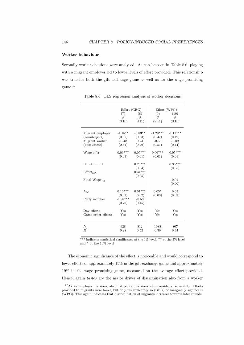
146 CHAPTER 8. POLICY-INDUCED SOCIAL PREFERENCES
Worker behaviour
Secondly worker decisions were analysed. As can be seen in Table 8.6, playing
with a migrant employer led to lower levels of effort provided. This relationship
was true for both the gift exchange game as well as for the wage promising
game.17
Table 8.6: OLS regression analysis of worker decisions
Effort (GEG) Effort (WPG)(7) (8) (9) (10)β β β β
(S.E.) (S.E.) (S.E.) (S.E.)
Migrant employer -1.15** -0.83** -1.29*** -1.17***(counterpart) (0.57) (0.33) (0.47) (0.42)Migrant worker -0.42 0.23 -0.65 -0.09(own status) (0.61) (0.29) (0.51) (0.44)
Wage offer 0.06*** 0.05*** 0.06*** 0.05***(0.01) (0.01) (0.01) (0.01)
Effort in t=1 0.26*** 0.35***(0.04) (0.05)
Effortlah 0.34***(0.05)
Final Wagelag 0.01(0.00)
Age 0.10*** 0.07*** 0.05* 0.03(0.03) (0.02) (0.03) (0.02)
Party member -1.98*** -0.53(0.70) (0.45)
Day effects Yes Yes Yes YesGame order effects Yes Yes Yes Yes
N 928 812 1088 807R2 0.28 0.52 0.30 0.44
*** indicates statistical significance at the 1% level, ** at the 5% leveland * at the 10% level
The economic significance of the effect is noticeable and would correspond to
lower efforts of approximately 15% in the gift exchange game and approximately
19% in the wage promising game, measured on the average effort provided.
Hence, again tastes are the major driver of discrimination also from a worker
17As for employer decisions, also first period decisions were considered separately. Effortsprovided to migrants were lower, but only insignificantly so (GEG) or marginally significant(WPG). This again indicates that discrimination of migrants increases towards later rounds.
8.5. DISCUSSION 147
perspective and differences in trust, which would play a bigger role in the wage
promising game, play a comparatively small role. In contrast to these results
depending on the status of the experimental counterpart, the worker’s own
hukou status did again not change the effort provided to the employer in a
statistically significant way. This insignificance, understood together with the
result on employer decisions shows that statistical discrimination cannot explain
why employers made lower offers to migrants, as own hukou status did not
change the effort decision.
The wage offer to participants was included as the main control variable.
The effect of the wage offer is significant and this effect is almost identical across
games. Additionally, the response to wage offers is close to an equilibrium: To
receive one more unit of effort, an employer would have to offer a wage increase
of 20, which corresponds to the extra profit the employer would earn from
this extra unit. Hence, employer offers are, on average, optimal given worker
responses.
Using the same reasoning as for employer decisions, age and party member-
ship were also included as further control variables, as these had been significant
for some of the specifications. However, due to the relatively low economic sig-
nificance of age and the small number of party members, they are not further
investigated here.
8.5 Discussion
Further interpretations
The experimental results showed that discrimination of migrant counterparts is
observable both from employers as well as from workers, but that own hukou
status does not lead to major changes in decisions. The implications of these re-
sults and their society-wide impact through the hukou system are less obvious.
And what is the impact of the system on individual attitudes when different
groups are dealing with each other in daily life? While the hukou system of-
ficially segregates Chinese citizens, official segregation does not automatically
have to lead to discrimination on an individual level. Nevertheless, official seg-
regation and discrimination might be interconnected; for example, segregation

148 CHAPTER 8. POLICY-INDUCED SOCIAL PREFERENCES
could sustain an (already existing) propensity to discriminate and exploit a
weaker social group if it legitimises discrimination or provides groups of people
with sufficient power to discriminate.18 In this sense discrimination that comes
as exploitation is observable.
As could be seen in the analysis, discrimination of the migrant group was
observable from employers as well as from workers. This indicates that discrim-
ination is independent of roles taken in the labour market and based on factors
such as lower preferences to cooperate with migrants, the conjecture that mi-
grants deserve to be worse off, or the assumption that they are more submissive
and content with smaller amounts. However, since migrants do not behave dif-
ferently than locals, discrimination just leads to lower levels of reciprocity and
less overall surplus available. Furthermore, the worse treatment of migrants
does also not seem to rely on statistical beliefs, or lower trust in migrants, as
discrimination again increased in the wage promising game when moving from
binding and up-front wages to ex post wage payments after observing effort.
Furthermore, the findings of this study also suggest that participants seem to
have adequate beliefs about likely (or maybe socially appropriate) reactions of
others, as average decisions seem to follow equilibrium response patterns, which
again suggests that tastes for discrimination, rather than statistical beliefs or
different trust in one of the groups drives behaviour. Again, these tastes can be
understood in a wider sense that may include social norms or the perception of
what is fair treatment of migrants. However, the results indicate that it is not
just something socially accepted by everyone to discriminate against migrants
(including migrants themselves), as it increases when wages are determined ex
post and when there is no risk any more that discrimination decreases own
outcomes through reduced reciprocity of the other player.
In the analysis of the experiment investigated two different games were cho-
sen to reflect different labour market contracts, one in which non-binding wage
offers are made, and one in which wage offers are binding. Allowing for non-
binding wage promises and allowing the employer to determine the final wage
at the end of the round leads to higher effort levels at slightly lower wages.
18The necessity to reach a certain income level through a limited number of income chan-nels available to the discriminated group could generate such a relationship when power isunequally distributed dependent on hukou status.

8.5. DISCUSSION 149
Cooperation between employers and workers remains high and even increases
with the introduction of wage promises. The reason for this is that employers
are able to use high wage offers as (true) positive signals. Locals and migrants
do not react differently to the two institutional frameworks; however, discrim-
ination of migrants significantly increases when non-binding promises become
possible, as the weaker bargaining position of workers is exploited more when
she is a migrant.
Another possible interpretation for what is observable is just different treat-
ments of in-group versus out-group members. For example, Ruffle and Sosis
(2006) report results from kibbutz members that are more cooperative amongst
themselves, but not different from normal citizens once they interact with these
other citizens. However, the hukou system segregates individuals only on the
basis of geographical characteristics and not on the wish to join a disadvan-
taged group, and for the experiments described here status was an essentially
exogenous factor. Furthermore, there is no reason to discriminate, as locals and
migrants are not fundamentally different. Nevertheless, the hukou system could
still be an in-group coordination device helping individuals to determine the
borders of their group. In any case, this still does not make the discrimination
of migrants based on the hukou system desirable.
Limitations
While the study allowed to derive interesting results, the approach also has clear
limitations. An occupational group of household aids was identified and their
behaviour studied in relation to participant’s hukou status. This group did lend
itself particularly well to being studied in the experiment, as being quite homo-
geneous across hukou groups and being unable to change their status. However,
it evidently remains an open question how one can generalise from the results
presented here to the general population and even to the general situation of
migrants in Nanjing. For example, for this low socio-economic group discrimi-
nation based on hukou status is likely to be more central than for the average
citizen. That is, if participants decide differently if they are more experienced in
the topic is a context-dependent empirical question (for example MBA students
with work experience were more willing to cooperate than undergraduates in a

150 CHAPTER 8. POLICY-INDUCED SOCIAL PREFERENCES
study by Hannan et al., 2002). Furthermore, tastes for discrimination can de-
pend on context, as even experiments on the easily observable attribute gender
have shown mixed results depending on the experimental framework (Eckel and
Grossman, 2008). However, the artefactual field experiment used in this study
can be regarded as an insightful approach studying this policy-relevant question
of the impact of the hukou system in this light. Nevertheless, more conservative
conclusions and interpretations restricted to the labour market, as done here,
are reasonable.
While experimental decisions were framed such that the descriptions were
more understandable for participants, a situation in which choices were com-
municated electronically between participants must have been unfamiliar to
participants who are employed in physical jobs and often had little experience
using computers. However, participants got through the experiment confidently
and relatively quickly and the share of strange decisions is not much higher than
is often observed when studying student populations.19
Finally, the experiment only allows to make statements about possible dis-
crimination once employers and workers with different hukou status actually
interact. However, discrimination might already take place earlier, for exam-
ple at the hiring level, reflecting what is commonly discussed on market level
effects of taste-based discrimination. For example, Slonim and Guillen (2010)
report experimental results indicating that discrimination mainly occurs when
individuals chose their partner of interaction.20 In the labour market of house-
hold aids, such discrimination probably takes place as well; i.e., agents that
were asked about this stated that about one third of clients request to hire only
locals.21 In this study individuals of different status were forced to interact in
the treatments, making it more difficult to predict how the behaviour observed
in the experiment can be representative of actual discrimination and if market
conditions lead to a long-term persistence or disappearance of discrimination
19Apparently, the definition of strangeness in decisions can be arbitrary; however, mostexperimenters will know that some participants follow decision patterns which are hard tomake sense of. In the games used here a high or maximum effort in response to a low orminimal wage offer would be a candidate for strange decisions.
20See also Bertrand and Mullainathan (2004), who study discrimination in hiring in a fieldexperiment using CVs.
21Reasons for this are usually the hope of hiring more civilised workers and individuals thathave similar preferences with respect to cooking styles; i.e. these are qualitative factors thatwere eliminated in the laboratory approach used here.

8.5. DISCUSSION 151
against migrants. However, results showed that the introduction of hukou sta-
tus has become a category of discrimination based on individual preferences, as
discrimination is the strongest in the WPG, where statistical characteristics or
unobservables that are correlated with the status of individuals are removed.
Furthermore, migrants usually do not take an employer role in reality and all
of the participants were used to being in the worker role. However, being able
to control for this counterfactual can also be seen as one of the advantages of
running experiments, allowing to observe attitudes that can be latent in reality.
Concluding remarks
As shown in the discussion of the analysis above, the study shows that migrants
are discriminated against. This is true although the experiment eliminates many
factors that might be the basis for discrimination in reality and that cannot
be captured in survey data, such as unobservable or perceived work quality.
The results indicate that discrimination is not based on different behaviour
of migrants. Hence, there is no objective reason for statistical discrimination.
Furthermore, discrimination also does not seem to be founded on (potentially
mistaken) beliefs about the trustworthiness of migrants - although lower trust
in migrants might also play a small role, at least judging by the increase of
discrimination from the worker side when moving to the wage promising game.
However, not much updating of beliefs about reactions of migrants and locals is
observable: Weak statistical significance in discrimination was seen in the first
period of the game. This significance increases when using all periods, and past
decisions of experimental counterparts do not have a significant influence on the
decision variables. Therefore, it seems that taste-based discrimination provides
the best explanation for observed behaviour.
The two different labour market frameworks show that migrants are discrim-
inated against and exploited more when employers can make non-binding wage
promises. This increases the undesirability of the hukou system, as (generally)
the introduction of non-binding wage promises increased efficiency in the sense
of more mutual surplus being created for employers and workers - even when
wages become binding in later periods, as employers and workers embark on a
152 CHAPTER 8. POLICY-INDUCED SOCIAL PREFERENCES
more cooperative path of positive reciprocity.22
Finally, the experimental results can be used to evaluate the hukou system.
The system had long been used to limit migration to urban areas by making
it less attractive for rural citizens to move and hukou status was used as the
official vehicle for this. However, the experimental results show that the system
also seems to have created motivations of individuals to discriminate against the
migrant group, probably by establishing a social perception that it is accept-
able to treat migrants less kind. However, disadvantaging migrants can create
discontempt and frustration among migrants, who do not seem to be fundamen-
tally different from locals; this frustration of migrants is unlikely to have been
desired by the hukou system.
But will just abolishing the official hukou system lead to disappearance of
discrimination? In a study using the Indian caste system, Hoff and Pandey
(2005) found that eliminating available information on caste status (of children
in an experiment) led to the elimination of behavioural differences. Similarly,
Afridi et al. (2010) applied the same experiment to Chinese school children us-
ing the hukou system instead of information on casts and come to a similar
conclusion. This gives rise to the assumption that official labelling of individ-
uals through the hukou system is actually a driver (and not just a mirror) of
discrimination. Results from this study support this view and give rise to the
hope that abolishing the system will also mediate individual-level discrimina-
tion, although it is well understood that positive effects through the reduction of
discrimination have to be weighed against other, potentially desirable elements
of the hukou system.
22The game order effect had a strong positive effect on wage offers in both games, leadingto higher wage offers throughout all periods when the wage promising game is played first.

Chapter 9
Overall implications for
social preferences of
individuals
The introduction to this part raised the question of what determines social pref-
erences, and how their shape might depend on strategic elements in the frame-
work of interaction. To study this question two experimental games, the GEG
and the WPG were used in two policy-oriented experimental studies using labour
market frameworks. In these labour market frameworks social preferences play
an important role in many applied contexts for generating mutual profits for
both sides of the labour market, because they rely on trusting attitudes and
reciprocity between employers and workers.
However, although both studies used the same experimental games, the out-
comes of the two studies were different. The first study showed that social
preferences of Australians did not depend on the characteristic of their counter-
part, as they made very similar offers to other Australians as they did to Asians,
or put formally in the framework of thinking βAustralians ≈ βAsians. This gen-
eral conclusion remained although the pattern of interaction between the two
groups changed when moving to the WPG. In the WPG promises played a differ-
ent role when made to Australians than when made to Asians. This indicates
153

154 CHAPTER 9. SOCIAL PREFERENCES CONCLUSION
that Asians are treated less kind by Australians (or βAustralians > βAsians),
but they were also rewarded more when positively reciprocating (indicating
βAustralians < βAsians). As both effects were of about the same size but in the
opposite direction, no general differences in social preferences were determinable.
Nevertheless, it was insightful to observe that the shape of the interactive frame-
work led to different patterns of reciprocity.
In contrast, similarity in social preferences depending on the characteris-
tic of the counterpart was not found in the second study, where the migrant
group was discriminated against, indicating βlocals > βmigrants. This statement
was true for both experimental games. Discrimination in wage offers decreased
when introducing non-binding wage promises, but increased in terms of realised
wages. This shows that different social preferences towards the two different
groups are observable and these preferences drive taste-based discrimination.
Indeed, as discrimination in the second study was strongest for final wages in
the WPG, it was not statistical discrimination that drove behaviour. As could
be seen in the results of the study, overstating own social preferences due to
reciprocity-concerns was observable: When the own outcome was still depen-
dent on the reciprocal decision of the counterpart, discrimination was reduced.
When lower wage offers were costly in terms of reducing the counterpart’s reci-
procity they were in a medium range. Discrimination was almost non-existent
when costly in reciprocity-terms, but not in outcome terms (i.e., in non-binding
wage promises). Finally, discrimination was at the highest level when costless
in reciprocity terms (as counterparts were not able to reciprocate unfavourable
treatment), but costly in outcome terms.
A second question and theme throughout this thesis was what role charac-
teristics of individuals played in decisions. For the first study this question was
investigated using extensive information from a pre-experimental questionnaire.
A first result of this procedure was that no strong selection into the experiment
out of the pool of students which were invited to experiment was observable.
However, some selection based on language abilities (which was experimenter-
induced) as well as based on some attitudinal factors played a role.
However, how important were any individual characteristics for experimental
decisions? Here the results showed that at least for the study included in the

155
first chapter no individual characteristic had a major impact on decisions taken
in the experiment. And if they had a statistically significant impact, they did
not drive the results found for any of the treatments. However, some attitudinal
characteristics did influence experimental decisions. In contrast, at least for the
subject pool studied, demographic characteristics such as gender and age (results
from this are not reported in the main results), but also cultural origin, did not
significantly change decisions. This conclusion also remained when including
fixed- and random- effects models to eliminate individual-level effects, as the
main results of the study remained.
Similarly, the statistical insignificance of the investigated status of being a
local or migrant was also found among participants in the second study. That is,
decision makers did not significantly differ in their choices based on whether they
were locals or migrants. With respect to other individual characteristics such
as age or gender this was, however, less clear and not always easy to interpret,
as the subjects were chosen to be relatively homogeneous.1 Nevertheless, there
was some indication that men are (statistically and economically) significantly
more selfish than women; the same was true for members of the communist
party. However, these (non-central) results were based on very small samples
and are therefore interpreted with care. Again, the overall effect of these fac-
tors on experimental results was small, but it indicates that some individual
characteristics may have a strong influence on how decisions are made in an
experimental setting. Nevertheless, using regression analysis that reduced the
individual effect did not invalidate the main results.
Finally, it is also interesting to consider the two economic experiments stud-
ied in this part as a policy evaluation tool. The first experiment used students
as experimental subjects which are most likely to be those to interact in the
future in the intercultural context studied. To understand the social interaction
between these two cultural groups, which is likely to be of growing importance
in the future, the experiment was a cheap tool to learn more about the speci-
ficities of their interaction. Similarly, the second study identified a subgroup
of the population that was particularly well-suited for studying the question at
hand. It found that hukou status as a public policy gave rise to taste-based dis-
1They were female except 3 male participants and had all the same occupation.

156 CHAPTER 9. SOCIAL PREFERENCES CONCLUSION
crimination, something not intended by the original introduction of the system.
Furthermore, it provided insights about how a public policy in general can be
used to shape individual-based preferences, which is an important and interest-
ing insight for policy-makers and complements other experimental studies on
labour market discrimination on the hiring level.

Part III
HRV as a relevance
indicator
157


Chapter 10
HRV as a relevance
indicator in the laboratory
and in reality
10.1 Introduction
As described in the introduction to this thesis, in the last decades behavioural
economists have increasingly become interested in the area of neuroeconomics, a
field trying to use neuroscientific data to inform economic analysis. First mile-
stones in this field have been an overview article by Camerer et al. (2005), the
book chapter by Egidi et al. (2008) and the book Neuroeconomics by Glimcher
et al. (2008). Since then various other studies have used neuroscientific tools
(mainly brain scans) to improve the understanding of economic decision mak-
ing. However, while providing interesting insights about processes in the brain
and the potential to localise social preferences (Fehr and Camerer, 2007; Fehr
et al., 2005; Quervain et al., 2004), risk and ambiguity attitudes (Hsu et al.,
2005; Huettel et al., 2006; Kuhnen and Knutson, 2005; McCoy and Platt, 2005;
Platt and Huettel, 2008) and time preferences (McClure et al., 2004; Kable
and Glimcher, 2007), the use of neuroeconomic tools has also limited research
opportunities in some ways. One such limit is that (particularly) brain scan-
159
160 CHAPTER 10. HRV IN THE LAB AND DAILY LIFE
ning techniques require extensive equipment, leading to the necessity of moving
studies increasingly into laboratory environments and out of field settings. As
economists are, however, interested in behaviour outside of the laboratory and
therefore often like to know about links to reality, studies with more connections
to the field are desirable. Examples for such attempts to move closer to the field
are field experiments on specific markets (e.g. List, 2006a; Marechal and Thoni,
2007) or laboratory- and field-based real effort experiments (e.g. Levitt and List,
2007; Hennig-Schmidt et al., 2010).
Linking laboratory-based measurements and measurements from the field is
particularly interesting if neuroeconomic data is interpreted as a relevance in-
dicator during the decision making process. Such an approach has been used
particularly in psychological research where psychological – that is mainly emo-
tional – significance is concluded from the significance of physiological measures
(Cacioppo and Tassinary, 1990). This approach has mainly been used con-
necting decisions in which emotions are involved to physiological data recorded
parallel to other observational data (e.g. Rohrmann and Hopp, 2008). Simi-
larly, it would be interesting to compare the physiologically-based relevance of
social preferences as compared to risk preferences. If thinking of the strength
of neuroscientific measures as mirroring an individual’s value function (such as
V (·) and O(·) in the overall framework of thinking used throughout this the-
sis), for example in terms of psychological costs and benefits, it would also be
interesting to relate the recorded signals during laboratory-based tasks to tasks
and decisions in real-life settings. This approach has been used in a number
of neuroeconomic studies, using brain signals as neural markers or value repre-
sentations in the brain (O’Doherty, 2004; Plassmann et al., 2007; Knoch et al.,
2010). To establish such a comparative link is the aim of this study which uses
heart rate variability (HRV) data as such a marker or indicator for (potentially
emotional) valuation, extending the realms of existing neuroeconomic studies to
what could potentially be described as physio-economics (Adam et al., 2011),
particularly in fields in which emotions play a role. HRV data can relatively
easily be collected in laboratory environments, and can also be recorded in the
field, because it does not require extensive recording equipment.
In order to compare laboratory results to field data, this study identifies
10.1. INTRODUCTION 161
a real-life event that is similar to a laboratory environment in which mainly
mental activity is exerted in relative silence and with predefined choice options.
For this a university exam was used. The physiological activity recorded dur-
ing the exam is consequently compared to physiological patterns during other,
less stressful mental activity and to the experiment, of which some parts were
designed to mimic the exam situation. Furthermore, the experiment includes
games to elicit social preferences and attitudes towards risk. To better un-
derstand the magnitude of experimental results and in order to get a better
picture of cross-individual heterogeneity in HRV, the study also collected data
of normal-day HRV activity of all participants over the course of 2 days. The
data from these measurements is subsequently used to compare HRV as a rel-
evance indicator during the experiment, comparing changes in HRV to their
corresponding changes based on experimental decisions and to its role as a rel-
evance indicator during daily activities. Furthermore, the study compares dif-
ferent preference types over risk and social attitudes. Throughout this analysis,
particular focus is put on an within-individual level of analysis.1
Results of the study show that physiological activity in the experiment, par-
ticularly in experimental tasks that resemble the exam task, and the exam are
similar. Within the experiment some decisions are connected to HRV when
social preferences play a role, while there is no clearly determinable connection
between HRV and risk taking in a gambling situation. This might be explained
by a higher emotional component of decisions that depend on social preferences.
Furthermore, the comparison of HRV as a relevance indicator in the experiment
and in reality shows that experimental effects are significant and support the
understanding that physiological data recorded in experiments includes valu-
able objective information that would correspond to significant physiological
processes in reality.
1Making within-subject comparisons is particularly relevant considering that some partic-ipants might be reacting stronger physiologically to any stressor, while showing only smallchanges in behaviour compared to other participants. This aspect of individual heterogeneitymight especially be relevant considering results reporting that changes in the HRV do nothave the same effects in terms of their magnitude across individuals (see, e.g. Crone et al.,2004).
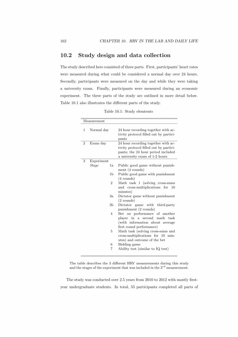
162 CHAPTER 10. HRV IN THE LAB AND DAILY LIFE
10.2 Study design and data collection
The study described here consisted of three parts. First, participants’ heart rates
were measured during what could be considered a normal day over 24 hours.
Secondly, participants were measured on the day and while they were taking
a university exam. Finally, participants were measured during an economic
experiment. The three parts of the study are outlined in more detail below.
Table 10.1 also illustrates the different parts of the study.
Table 10.1: Study elemtents
Measurement
1 Normal day 24 hour recording together with ac-tivity protocol filled out by partici-pants
2 Exam day 24 hour recording together with ac-tivity protocol filled out by partici-pants; the 24 hour period includeda university exam of 1-2 hours
3 ExperimentStage 1a Public good game without punish-
ment (4 rounds)1b Public good game with punishment
(4 rounds)2 Math task 1 (solving cross-sums
and cross-multiplications for 10minutes)
3a Dictator game without punishment(2 rounds)
3b Dictator game with third-partypunishment (2 rounds)
4 Bet on performance of anotherplayer in a second math task(with information about averagefirst round performance)
5 Math task (solving cross-sums andcross-multiplications for 10 min-utes) and outcome of the bet
6 Bidding game7 Ability test (similar to IQ test)
The table describes the 3 different HRV measurements during this studyand the stages of the experiment that was included in the 3rd measurement.
The study was conducted over 2.5 years from 2010 to 2012 with mostly first-
year undergraduate students. In total, 55 participants completed all parts of

10.2. STUDY DESIGN AND DATA COLLECTION 163
the study. Additionally, 2 participants took part in the experiment, but were
not measured during the exam. Furthermore, for 1 participant decision times
during the experiment were not recorded. Together this results in samples of 56
participants for experimental decisions and between 46 and 54 participants for
decisions linking out-of-laboratory with laboratory findings.2 For their partici-
pation in the study participants received 50 Australian dollars (fixed amount)
for the two 24-hour measurements and, on average, 24 Australian dollars de-
pending on their decisions and performance in the experiment, which typically
lasted for 80 minutes.
10.2.1 Measurements over 24 hours
In the two measurements over 24 hours participants arranged an individual time
with the experimenter to start their measurement. They were handed a heart
rate monitor, attached the 3 electrodes of the monitor to their chest in private
and started the measurement. The quality of the recording was tested using
an infrared connector to the heart rate monitor. Participants were handed a
template activity protocol (see appendix) which they were asked to fill out.
They were told that the protocol would have to be filled out depending on
their activities during the day, recording major changes in activities (such as
studying, walking, eating, sleeping, watching TV, etc.). It was further pointed
out to them that a minimum time interval useful for the analysis was around
5 minutes and that longer activities lasting for hours would be acceptable in
terms of the detail required for this study.
Measurement on the normal day
The measurement of participants on the normal day aimed to allow subjects
to get used to the monitoring device and to make sure that they would be
comfortable wearing the device on the exam day. Participants were also given
the opportunity to drop out of the study after this first measurement. Two
participants did so explicitly and others missed their appointment on the exam
day. However, most participants that started also completed the study. They
2The sample was reduced, for example as not all participants recorded to have done com-puter work during their 24-hour measurements.

164 CHAPTER 10. HRV IN THE LAB AND DAILY LIFE
also reported that the monitor was not noticeable few minutes after attaching it
and that it did not change normal activity patterns during the day. The other
reason for the normal day measurement was that it allowed to observe partici-
pants over various activities and provided a potential baseline for analysing and
understanding HRV measurements during the exam and the laboratory exper-
iment. For this reason participants were asked to behave as they would have
done on any other day.
Measurement on the exam day
The measurement of participants on the exam day was interested in the stress
level of participants during the exam. It also provided additional information
about the HRV level for activities that could be compared to the exam measure-
ment. Practically, participants were allowed to schedule the exam day session
(i.e., 24 hours) as they preferred, but were required to continue the measure-
ment until one hour after the exam to observe possible cooling-down effects.
The exams lasted generally one hour, although participants wore the monitor in
different exams. However, these exams were relatively comparable as almost all
were undergraduate business exams, they had to last between 1 and 2 hours and
had to count between 40% and 60% of the final grade of the subject. As such the
exam is seen as reflecting a relatively intense and potentially stressful mental
activity in a controlled environment similar to a laboratory. This resulted in
hypothesising that physiological activity would be higher than during every-day
mental activity, with the difference between these two providing a benchmark
for HRV changes in laboratory-based measures.
10.2.2 Measurement during an economic experiment
The third measurement was recorded during an economic experiment. The ex-
periment was implemented in a computer laboratory using z-Tree (Fischbacher,
2007). After the completion of the first two parts of the study, participants
were contacted individually via e-mail and experimental sessions were sched-
uled such that always multiples of 3 participants were required for one session.
In order to gain a better understanding of which experimental elements were
best comparable to the exam, a number of different games and specifications

10.2. STUDY DESIGN AND DATA COLLECTION 165
were played. After participants had entered their participant number, the games
and tasks were presented to the participants in a succession of 7 stages as de-
scribed below. Of these, the first 6 were payment-relevant. In the 7th and last
stage participants were only informed about their score, but not paid based on
their performance. Furthermore, in the first 6 stages instructions were read out
aloud by the experimenter, while in the last stage participants were asked to go
through the instructions privately.3 The first 6 stages were treated differently
from the 7th stage as representing experimental standards in economics and
psychological research. Experimental payoffs of the first 6 stages were calcu-
lated in experimental dollars that paid 20 experimental dollars = 1 Australian
dollar as announced in the beginning of the experiment. The full instructions
are included in the appendix.
Stage 1: Public good game (PGG)
In the first stage, participants played a standard public good game (PGG), which
has extensively been studied in the experimental economic literature since the
first far-reaching article published by Marwell and Ames (1981). In this game,
participants have a certain amount which they can use to contribute to a public
good. The public good is available to a group of other participants (and usually
also to the decision maker). However, as contributions are more costly than the
benefit received from the own contribution, selfish payoff-maximizing players
will contribute nothing. Assuming all players with such motives will lead to an
equilibrium outcome with no contributions, the socially worst outcome.
Formally, the PGG is usually described as follows. Each participant receives
an endowment of ωPGGi which can be kept for private use or contributed as
xPGGi ≤ ωPGGi to a public good. The public good is shared with n other
players. All n players benefitting from the public good have a payoff function
of
πPGGi = ωPGGi − xPGGi + λ
3∑j=1
xPGGj
with 1n < λ < 1 indicating positive contributions generate social gains, while
3Stages 2 and 5 had identical instructions; this was pointed out to participants in stage 5while the full instructions were not repeated in full.
166 CHAPTER 10. HRV IN THE LAB AND DAILY LIFE
own contributions xPGGi are costly for each contributor.
For the implementation in this study participants were provided with an
endowment of ωPGGi =10 experimental dollars, which they could keep or con-
tribute to a public good that was shared in a group of three participants. All
contributions made to this public good were multiplied by the factor 2, added
up and redistributed equally to the members of the group (hence λ = 23 ). Re-
sults from this game are usually interpreted in the context of cooperation and
high contributions interpreted as a higher willingness to sacrifice own resources
for common use. A common characteristic of this game is that contributors
are anonymous and it is not possible to observe which group member has con-
tributed which amount. With those specifications, the PGG was played for 4
rounds.
Afterwards a modification of the game was played in which participants, after
all group members had made their contributions, were able to observe who had
contributed which amount. They were then able to punish other players for
their decisions (independent of whether and how much they had contributed).
A punishment resulted in a situation where the punishing player had to incur a
costij of 2 experimental dollars per punished player j and punished players had
to pay a fineji of 4 experimental dollars for every player j that had punished
the decision maker. The payoff function hence changes to
πPGGi = ωPGGi − xPGGi + λ
3∑j=1
xPGGj −∑i
costij −∑j
fineji.
Results from various studies in the literature have shown that the presence
of punishment opportunities can lead to increased contribution levels and that
punishment is exerted towards free-riders although being costly to the enforcer
(Fehr and Gachter, 2000, 2005; Herrmann et al., 2008). The aim of this variant
of the game was particularly designed in order to observe if potential punish-
ments (for punishers or receivers) had effects on the stress level of participants
involved in the experiment. This second variant of the PGG was again repeated
for 4 rounds. It was hypothesised that higher contributions would be paralleled
by increase physiological activity, reflecting that pro-social choices are partly
motivated by social norms, which are connected to emotions. A similar argu-
10.2. STUDY DESIGN AND DATA COLLECTION 167
ment was assumed for punishment decisions (also see Dulleck et al., 2012b).
Stage 2: Math task part 1
In the following stage of the experiment, participants were asked to solve 20
arithmetic questions within a time limit of 10 minutes. Half of the questions were
asking participants to solve cross-sums (345 would be 3+4+5=12), the other half
were asking participants to solve cross-multiplications (345 would be 3*4*5=60)
without the use of pen and paper. Whether cross-sums or cross-multiplications
had to be answered changed between periods. Questions were increasing in
difficulty over time, whereas the first questions were simple, while later ones
were very hard to solve (even math-affine PhD students were struggling to solve
them without pen and paper within a short time-frame). For every question
correctly answered, students received 8 experimental dollars. The aim of this
part of the experiment was to determine whether this task was comparable to
HRV patterns that were observable in the exam. For this and the two other
effort-requiring tasks (see description below) it was hypothesised that higher
effort and a higher score would be reflected in higher physiological activity. It
was also hypothesised that the tasks would be most highly correlated (within
individual) to the exam measure.
Stage 3: Dictator game (DG)
In the next stage of the experiment, students played the so-called dictator game
(DG). See Engel (2011) for a review of the literature and a meta-analysis. In
this game, two players are matched with each other, one being the transferring
player, the dictator, and the other the recipient. The dictator can transfer any
fraction of an amount of her endowment ωDGi to the recipient and is not com-
pensated for this transfer. This will lead payoff-maximizing players to transfer
nothing. Results that show positive transfers (the literature usually reports val-
ues commonly close to half of ωDGi ) are usually interpreted as social preferences
of the dictators or such that their behaviour reflects conforming to social norms
about fair shares.
In the experiment here, the dictators were provided with an endowment of
ωDGi =10 experimental dollars. The transferring player was able to decide on
168 CHAPTER 10. HRV IN THE LAB AND DAILY LIFE
the allocation of ωDGi , which means that any share between 0 and 10 (in steps
of 1 experimental dollar) could be transferred to the recipient. The recipient
was passive and did not have the possibility to communicate anything back to
the transferring player. The aim of this game was to determine if having to
decide on social allocations mattered for the HRV of the participants. Any such
information would provide with insight of how for example social preferences or
the necessity to conform to social norms matter for stress levels of participants.
This standard version of the game was played for 2 rounds.
In a second step, the game was modified such that after the transfer to the
recipient had been made, a third player that was unaffected by the transaction
had the possibility to evaluate the transaction and to punish the transferring
player if wanted. Again, a fine of 4 experimental dollars was imposed on the
punished player and punishing had a cost of 2 experimental dollars. This mod-
ification was again repeated for 2 rounds. The aim was again to determine
if e.g. social preferences over allocations between third parties lead to differ-
ent HRV patterns. As for PGG decisions, increased physiological activity was
hypothesised to parallel more pro-social decisions.
Stage 4: Betting game
In the next stage of the experiment participants were informed that in the
following stage they would again solve math questions as they did earlier in the
experiment. They were provided with 30 experimental dollars which they were
allowed to bet on the performance of another player who had been randomly
assigned to them. The bet was on how many answers this assigned player
would (at least) answer correctly. Participants were informed about the average
performance of all participants in the first round of question-solving, but no
information on the assigned player was provided. Table 10.2 shows the betting
odds as presented to participants. The aim of the game was to determine if the
betting behaviour or the observation of the betting outcome had any impact on
the HRV. It was hypothesised that more (physiologically) stressed participants
would be more cautious when making their bets (as of the results in chapter 4).

10.2. STUDY DESIGN AND DATA COLLECTION 169
Table 10.2: Table of betting odds for participants
Number of Factor multipliedcorrect answers with 30 in
case of winning4 1.28 1.510 212 2.514 316 418 620 10
Stage 5: Math task part 2
The second arithmetic task had the same structure as before. Additionally, at
the end of the task, participants were informed about the outcome of their bet
made in the previous stage.
Stage 6: Bidding game (BG)
In the next stage participants were provided with an endowment of ωBGi =10
experimental dollars in every round, which they were able to keep or use to bid
xBGi for a common pot. The value of this pot was unknown to participants, as
it consisted of the bids placed by all bidders (again groups of three players were
forming a group) as well as 10 additional experimental dollars that were always
part of the pot. The allocation of the pot was determined by the ranking of the
bids: The player with the highest bid received 12 of the total amount in the pot,
the player with the second highest bid 13 and the player with the lowest bid 1
6 .
In case of equal bids, players equally shared what they would have won jointly.
Formally, the payoff function can be described as follows (in case there was no
tie):
πBGi = ωBGi − xBGi + νi(10 +
3∑j=1
xBGj );
with νi depending on the rank of i in the bids. The game does not have
an equilibrium in pure strategies, as the incentives are such that outbidding
other players is optimal until the maximum is reached. At this maximum point,
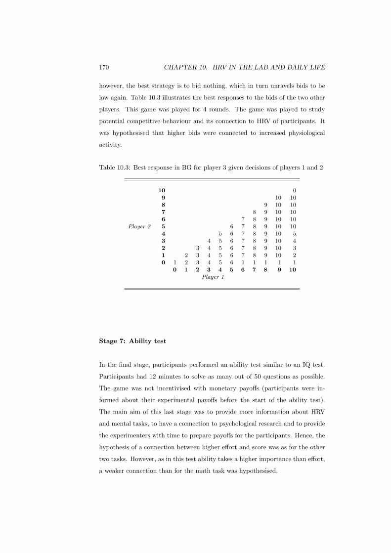
170 CHAPTER 10. HRV IN THE LAB AND DAILY LIFE
however, the best strategy is to bid nothing, which in turn unravels bids to be
low again. Table 10.3 illustrates the best responses to the bids of the two other
players. This game was played for 4 rounds. The game was played to study
potential competitive behaviour and its connection to HRV of participants. It
was hypothesised that higher bids were connected to increased physiological
activity.
Table 10.3: Best response in BG for player 3 given decisions of players 1 and 2
10 09 10 108 9 10 107 8 9 10 106 7 8 9 10 10
Player 2 5 6 7 8 9 10 104 5 6 7 8 9 10 53 4 5 6 7 8 9 10 42 3 4 5 6 7 8 9 10 31 2 3 4 5 6 7 8 9 10 20 1 2 3 4 5 6 1 1 1 1 1
0 1 2 3 4 5 6 7 8 9 10Player 1
Stage 7: Ability test
In the final stage, participants performed an ability test similar to an IQ test.
Participants had 12 minutes to solve as many out of 50 questions as possible.
The game was not incentivised with monetary payoffs (participants were in-
formed about their experimental payoffs before the start of the ability test).
The main aim of this last stage was to provide more information about HRV
and mental tasks, to have a connection to psychological research and to provide
the experimenters with time to prepare payoffs for the participants. Hence, the
hypothesis of a connection between higher effort and score was as for the other
two tasks. However, as in this test ability takes a higher importance than effort,
a weaker connection than for the math task was hypothesised.
10.3. EXPERIMENTAL RESULTS 171
10.3 Experimental results
For the analysis of the experimental data, decisions made during the games were
joined with the HRV measures. This was done such that for every decision made
the HRV recorded in an interval of 10 seconds on each side of the measurement
was assigned to an experimental decision.4 Subsequently, for each individual,
HRV measures from activities of the 24-hour measurements were added to the
experimental data.5 From this 24-hour measurement data the most common
activities were investigated. These were the exam, mental activity, computer
work, sleeping, watching TV, walking or cycling, resting or relaxing, eating and
drinking, communication, using public transport and driving. The following
paragraphs describe the general analysis of the experiment, its connection to the
exam and to other out-of-laboratory activities. Following this, more detail and
analysis on the specific games that were played in the course of the experiment
is included.
10.3.1 Connection between the experiment and the exam
One first conjecture of adding exam data to experimental data was to scrutinise
if the physiological state during the exam and the experiment were similar,
compared to the physiological state during other activities. Table 10.4 shows
the correlations of the HRV during different experimental games, the exam and
other activities. As can be seen, the correlations between the HRV during
experimental tasks and during the exam is significant. A similar and partly
stronger result is observable for other activities that would also be comparable
to the experiment, like mental activity or computer work. Other activities, in
contrast, appear to be unrelated to the experiment, such as sleeping or relaxing.
Table 10.4 illustrates these correlations.
4Practically, every event in the experiment, such as entering a screen or clicking the OKbutton was recorded with its corresponding time. These events were then matched to theHRV data such that the event time served as the midpoint of a 20 second interval. Theanalysis below used the moment of clicking the ok button as the event to be linked to thedecision. Furthermore, a second measure was used, i.e. the average HRV during which adecision was made from entering the decision screen to leaving it. Alternative events wereused to corroborate the results described in the description below. There were no qualitativechanges on results reported here.
5For this the averaged HRV over the complete time of the activity as recorded in theactivity protocol was used.
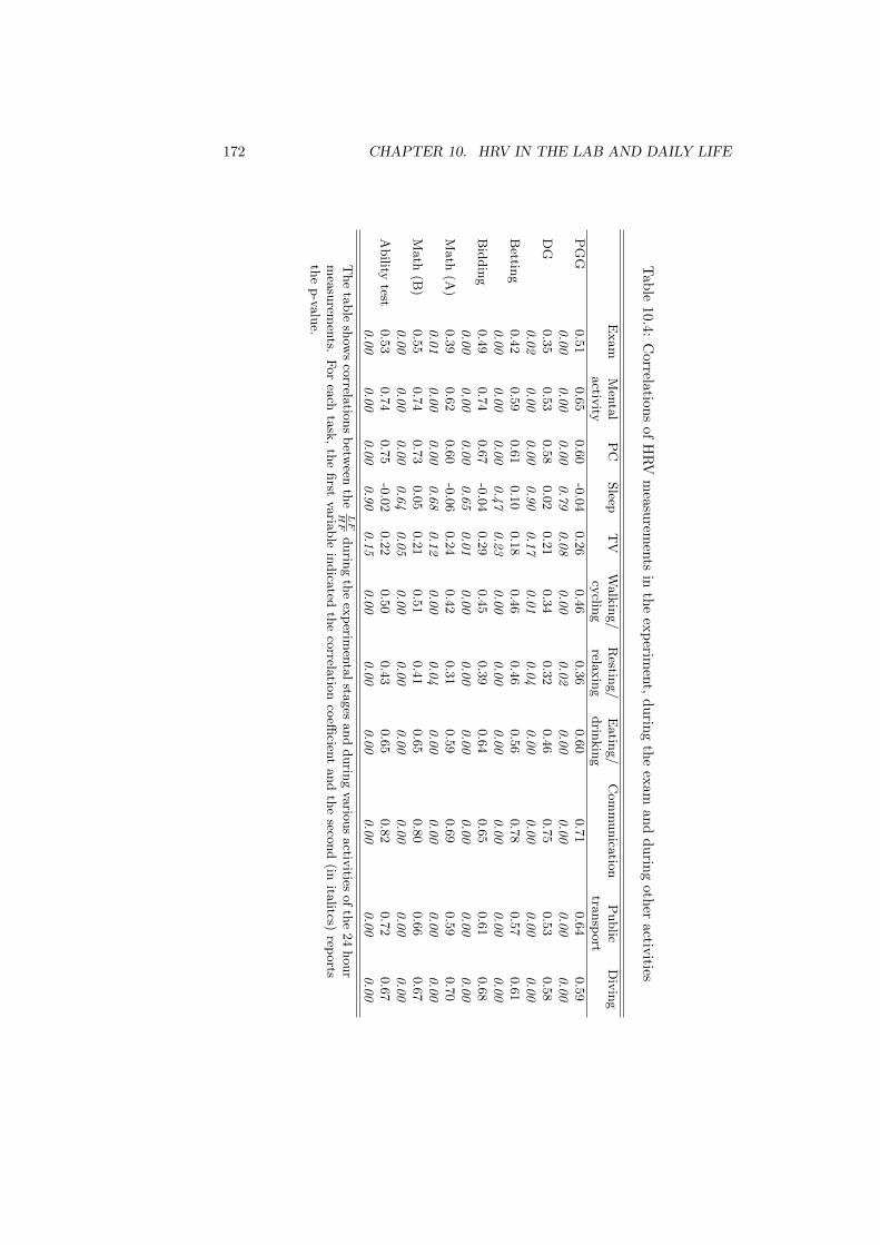
172 CHAPTER 10. HRV IN THE LAB AND DAILY LIFE
Tab
le10.4:
Correla
tions
ofH
RV
mea
surem
ents
inth
eex
perim
ent,
du
ring
the
exam
and
du
ring
other
activities
Exam
Men
tal
PC
Sleep
TV
Walk
ing/
Restin
g/
Eatin
g/
Com
munica
tion
Public
Div
ing
activ
itycy
cling
relaxin
gdrin
kin
gtra
nsp
ort
PG
G0.5
10.6
50.6
0-0
.04
0.2
60.4
60.3
60.6
00.7
10.6
40.5
90
.00
0.0
00
.00
0.7
90
.08
0.0
00
.02
0.0
00
.00
0.0
00
.00
DG
0.3
50.5
30.5
80.0
20.2
10.3
40.3
20.4
60.7
50.5
30.5
80
.02
0.0
00
.00
0.9
00
.17
0.0
10
.04
0.0
00
.00
0.0
00
.00
Bettin
g0.4
20.5
90.6
10.1
00.1
80.4
60.4
60.5
60.7
80.5
70.6
10
.00
0.0
00
.00
0.4
70
.23
0.0
00
.00
0.0
00
.00
0.0
00
.00
Bid
din
g0.4
90.7
40.6
7-0
.04
0.2
90.4
50.3
90.6
40.6
50.6
10.6
80
.00
0.0
00
.00
0.6
50
.01
0.0
00
.00
0.0
00
.00
0.0
00
.00
Math
(A)
0.3
90.6
20.6
0-0
.06
0.2
40.4
20.3
10.5
90.6
90.5
90.7
00
.01
0.0
00
.00
0.6
80
.12
0.0
00
.04
0.0
00
.00
0.0
00
.00
Math
(B)
0.5
50.7
40.7
30.0
50.2
10.5
10.4
10.6
50.8
00.6
60.6
70
.00
0.0
00
.00
0.6
40
.05
0.0
00
.00
0.0
00
.00
0.0
00
.00
Ability
test0.5
30.7
40.7
5-0
.02
0.2
20.5
00.4
30.6
50.8
20.7
20.6
70
.00
0.0
00
.00
0.9
00
.15
0.0
00
.00
0.0
00
.00
0.0
00
.00
The
table
show
sco
rrelatio
ns
betw
eenth
eLF
HF
durin
gth
eex
perim
enta
lsta
ges
and
durin
gva
rious
activ
itiesof
the
24
hour
mea
surem
ents.
For
each
task
,th
efirst
varia
ble
indica
tedth
eco
rrelatio
nco
efficien
tand
the
second
(inita
litcs)rep
orts
the
p-va
lue.

10.3. EXPERIMENTAL RESULTS 173
For some activities that are correlated to the activity in the experiment the
correlation is stronger than the correlation of the exam and the experiment. This
indicates that the exam is not the only comparable activity to the experiment
in terms of physiological states. However, this is not necessarily a negative
result, as in these other activities similarly stressful decisions with economic
consequences are taken. For example, the strong correlation to physiological
activity during communication seems desirable when studying social preferences
which played a role in two of the games studied here.
In this context, the results presented in Table 10.4 also inform about the
degree of correlation of the different experimental tasks and games to the exam
(and other activities). Within the experiment it appears that the tasks, par-
ticularly the second math task and the ability test are most comparable to the
exam and to other activities outside of the laboratory.
At the same time it is surprising that – generally – high correlations for
almost all activities and the exam are observable. A main reason for this is
a high heterogeneity in HRV measures across individuals, which leads to the
observation that HRV is not easily comparable across individuals. This leads
to the result that different activities, like computer work and driving (and also
decisions during the experiment) do not appear to be significantly different
from one another unless there are some decisions or activities that have a very
strong effect on physiological activity. Figure 10.1 illustrates this observation,
of seemingly insignificant results in HRV across individuals. For this reason the
following analysis describes the connection of HRV measures and experimental
decisions on two levels and reporting different alternatives. The first level uses
direct LFHF -results, values standardised by individual, as well as standardised by
24-hour activities (the exam, mental activity and sleep).6 However, on this first
level no clear differences across individuals could be determined. The results
reported therefore refer to the second level which uses individual-fixed effects
models to analyse experimental decisions to account for individual heterogeneity.
This is done assuming that any connection between HRV and experimental
decisions should at least be apparent in this type of within-individual analysis.
6Normal standardisation is done usingLFHF
sd( LFHF
)and standardisation by activities through
usingLFHF
activity−mean( LFHF
)

174 CHAPTER 10. HRV IN THE LAB AND DAILY LIFE
Figure 10.1: Distributions of LFHF -values over different activities during the 24-
hour measurements
05
10
15
20
LF
/HF
bus, m
etro
, ect.
com
mun
icat
ion
com
pute
r wor
k
driving
eatin
g/dr
inking
exam
men
tal a
ctivity
slee
p tv
walking
/cyc
ling
Again, on this second level the same alternative specifications for the HRV as
before were used to check for the robustness of results. The following sections
will describe cross-individual comparisons and then move to further analysis
of within-individual relationships of HRV and experimental decisions for which
significant relationships can be determined.
10.3.2 Measure of the magnitude of changes in HRV
HRV data measured outside of the laboratory can also be used for some further
analysis in connection to the games. The exam, as compared to other actives
during the 24-hour period, was usually more stressful within individuals when
being compared to other, primarily mental activities. The exam was assumed
to be more stressful, based on a study done on medical students (Lucini et al.,
2002) that recorded the HRV of students on the day of their medical exam and
compared this to a control day. This study found higher stress in the hour before
taking the exam. Table 10.5 confirms these findings and illustrates this for com-
parisons based on HRV between the exam and other daytime activities which
imply some minor physiological stress, i.e. computer work, mental activity and

10.3. EXPERIMENTAL RESULTS 175
Table 10.5: HRV differences between the exam and other activities
Exam – Exam – Exam –mental activity computer work communication
Exam 0.45*** 0.27* 0.52***(0.17) (0.16) (0.19)
Individual Effects Yes Yes Yes
N 208 343 145R2 0.577 0.488 0.734
The table reports results from fixed-effects regressions of the exam on HRV for otheractivities during the 24-hour period. Standard errors (clustered by individuals) areincluded in brackets. *** indicates 1% significance, ** 5% significance and * 10%significance.
communication.7 Hence, the coefficients in Table 10.5 on the exam variable pro-
vide an idea about the magnitude of changes in terms of the HRV indicator LFHF
between these normal activities and the exam. As can be seen in the regression
Table 10.5, the exam was, once controlling for individual heterogeneity in the
HRV, significantly more stressful (in the sense of implying higher HRV activity)
than other mental activity. The table also includes comparisons of the exam and
other activities that might potentially be comparable to the exam and of which
a large enough number of participant recordings during the 24-hour measure-
ment were available. As can be seen in these other comparisons, computer work
appeared to be more stressful and closer to the exam, although still less stress-
ful. Conversely, communication (covering mainly longer phone calls) appeared
to be less stressful than the other activities and most different from the exam.
Furthermore, these results put changes in HRV based on experimental decisions
into perspective in terms of their physiological magnitude (or economic signif-
icance), although a direct interpretation of the coefficients’ magnitude seems
difficult as describing changes within (heterogeneous) individuals.
10.3.3 Relationships between the experimental parts
In a first step of analysis within the experiment connections between the different
parts of the game were analysed. Table 10.6 shows correlations between the
different decision variables and the number of correct answers during the two
7Other activities, such as walking and cycling or using public transport are often morestressful than the exam in a physiological sense as they do not only reflect mental activity.
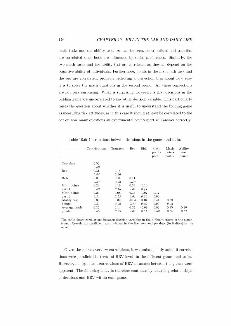
176 CHAPTER 10. HRV IN THE LAB AND DAILY LIFE
math tasks and the ability test. As can be seen, contributions and transfers
are correlated since both are influenced by social preferences. Similarly, the
two math tasks and the ability test are correlated as they all depend on the
cognitive ability of individuals. Furthermore, points in the first math task and
the bet are correlated, probably reflecting a projection bias about how easy
it is to solve the math questions in the second round. All these connections
are not very surprising. What is surprising, however, is that decisions in the
bidding game are uncorrelated to any other decision variable. This particularly
raises the question about whether it is useful to understand the bidding game
as measuring risk attitudes, as in this case it should at least be correlated to the
bet on how many questions an experimental counterpart will answer correctly.
Table 10.6: Correlations between decisions in the games and tasks
Contributions Transfers Bet Bids Math Math Abilitypoints points testpart 1 part 2 points
Transfers 0.530.00
Bets 0.31 0.150.02 0.26
Bids 0.08 0.3 0.110.57 0.02 0.43
Math points 0.29 0.19 0.34 -0.10part 1 0.03 0.16 0.01 0.47Math points 0.20 0.08 0.33 -0.07 0.77part 2 0.14 0.53 0.01 0.60 0.00Ability test 0.33 0.32 -0.04 0.16 0.41 0.28points 0.01 0.02 0.77 0.23 0.00 0.04Average math 0.26 0.14 0.35 -0.09 0.93 0.95 0.36points 0.05 0.29 0.01 0.51 0.00 0.00 0.01
The table shows correlations between decision variables in the different stages of the exper-iment. Correlation coefficient are included in the first row and p-values (in italitcs) in thesecond.
Given these first overview correlations, it was subsequently asked if correla-
tions were paralleled in terms of HRV levels in the different games and tasks.
However, no significant correlations of HRV measures between the games were
apparent. The following analysis therefore continues by analysing relationships
of decisions and HRV within each game.
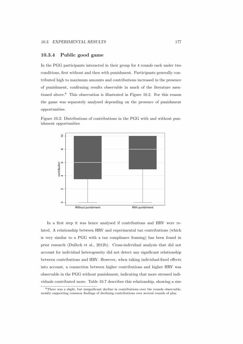
10.3. EXPERIMENTAL RESULTS 177
10.3.4 Public good game
In the PGG participants interacted in their group for 4 rounds each under two
conditions, first without and then with punishment. Participants generally con-
tributed high to maximum amounts and contributions increased in the presence
of punishment, confirming results observable in much of the literature men-
tioned above.8 This observation is illustrated in Figure 10.2. For this reason
the game was separately analysed depending on the presence of punishment
opportunities.
Figure 10.2: Distributions of contributions in the PGG with and without pun-ishment opportunities
02
46
810
contr
ibution
Without punishment With punishment
In a first step it was hence analysed if contributions and HRV were re-
lated. A relationship between HRV and experimental tax contributions (which
is very similar to a PGG with a tax compliance framing) has been found in
prior research (Dulleck et al., 2012b). Cross-individual analysis that did not
account for individual heterogeneity did not detect any significant relationship
between contributions and HRV. However, when taking individual-fixed effects
into account, a connection between higher contributions and higher HRV was
observable in the PGG without punishment, indicating that more stressed indi-
viduals contributed more. Table 10.7 describes this relationship, showing a size
8There was a slight, but insignificant decline in contributions over the rounds observable,weakly supporting common findings of declining contributions over several rounds of play.
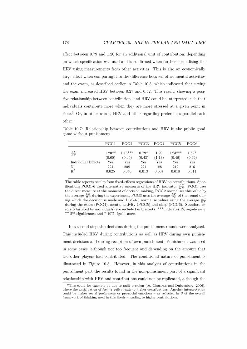
178 CHAPTER 10. HRV IN THE LAB AND DAILY LIFE
effect between 0.79 and 1.20 for an additional unit of contribution, depending
on which specification was used and is confirmed when further normalising the
HRV using measurements from other activities. This is also an economically
large effect when comparing it to the difference between other mental activities
and the exam, as described earlier in Table 10.5, which indicated that sitting
the exam increased HRV between 0.27 and 0.52. This result, showing a posi-
tive relationship between contributions and HRV could be interpreted such that
individuals contribute more when they are more stressed at a given point in
time.9 Or, in other words, HRV and other-regarding preferences parallel each
other.
Table 10.7: Relationship between contributions and HRV in the public goodgame without punishment
PGG1 PGG2 PGG3 PGG4 PGG5 PGG6
LFHF
1.20** 1.16*** 0.79* 1.29 1.23*** 1.82*(0.60) (0.40) (0.43) (1.13) (0.46) (0.99)
Individual Effects Yes Yes Yes Yes Yes Yes
N 224 208 224 188 212 216R2 0.025 0.040 0.013 0.007 0.018 0.011
The table reports results from fixed-effects regressions of HRV on contributions. Spec-ifications PGG1-6 used alternative measures of the HRV indicator LF
HF. PGG1 uses
the direct measure at the moment of decision making, PGG2 normalises this value bythe average LF
HFduring the experiment, PGG3 uses the average LF
HFof the round dur-
ing which the decision is made and PGG4-6 normalise values using the average LFHF
during the exam (PGG4), mental activity (PGG5) and sleep (PGG6). Standard er-rors (clustered by individuals) are included in brackets. *** indicates 1% significance,** 5% significance and * 10% significance.
In a second step also decisions during the punishment rounds were analysed.
This included HRV during contributions as well as HRV during own punish-
ment decisions and during reception of own punishment. Punishment was used
in some cases, although not too frequent and depending on the amount that
the other players had contributed. The conditional nature of punishment is
illustrated in Figure 10.3. However, in this analysis of contributions in the
punishment part the results found in the non-punishment part of a significant
relationship with HRV and contributions could not be replicated, although the
9This could for example be due to guilt aversion (see Charness and Dufwenberg, 2006),where the anticipation of feeling guilty leads to higher contributions. Another interpretationcould be higher social preferences or pro-social emotions – as reflected in β of the overallframework of thinking used in this thesis – leading to higher contributions.

10.3. EXPERIMENTAL RESULTS 179
direction of the within-individual relationship remained the same (but was in-
significant).10
Figure 10.3: Average punishment by contribution level in the PGG
02
46
8M
ean p
unis
hm
ent by c
ontr
ibution
0 1 2 3 4 5 6 7 8 9 10
Furthermore, also the connection between own punishment and the effect of
being punished was studied. However, the connection between these and HRV
was mostly insignificant, with only some weak indication that being punished
was negatively associated with HRV. As this second result was dependent on
the HRV measure used and was not a stable result, no further emphasis was
put on it, as a clearly determinable relationship appears insufficiently robust to
slight variation in the specification used in the analysis.
10.3.5 Dictator game
The DG was also played in the two no-punishment conditions followed by a
punishment condition. As illustrated in Figure 10.4 the presence of punish-
ment raised the level of pro-social behaviour. It is surprising to see that in
both conditions a noticeable number of self-sacrificing individuals exist, hence
individuals who allocate more than half of their endowment to an experimental
10This might potentially be driven by a crowding out of own positive emotions when con-tributing or the fact that in the presence of punishment opportunities also more selfish indi-viduals contribute moderate to high amounts to avoid being punished.

180 CHAPTER 10. HRV IN THE LAB AND DAILY LIFE
counterpart.11
Figure 10.4: Distributions of contributions in the DG with and without punish-ment opportunities
02
46
810
transfe
r
Without punishment With punishment
Linking the decisions over transfers and HRV does not show significant re-
sults, neither when looking across individuals nor when taking individual het-
erogeneity into account. Furthermore, this observation was true for both the
no-punishment and the punishment condition, although the direction of any
effect was again the same to the one observable in the PGG.12
Furthermore, it was analysed if punishment, which was in this case done by
a third party, was linked to HRV. Although the punisher was not personally
affected by the transfer and even incurred a cost when punishing, punishments
of low transfers can be observed, as illustrated in Figure 10.5. While observ-
ing the result that receiving punishment was not related to HRV, there was a
significant relationship between HRV and the decision to punish others for the
third party punisher. Table 10.8 illustrates this relationship, indicating that
higher physiological activity implies a higher probability to punish. This again
might reflect emotional pro-social attitudes motivating the decision to punish,
11For this reason only individuals that contributed half of their endowment or less wereanalysed separately. However, there was no significant change in results observable.
12One reason for this difference might be the relatively small number of within-condition andwithin-individual decisions in the DG studied here. Furthermore, a significant effect could beshown for transfers in the punishment condition when using exam-normalised HRV-measures.However, as this result was not robust across different specifications, it is not emphasised here.

10.3. EXPERIMENTAL RESULTS 181
Figure 10.5: Average punishment by transfer level in the DG
01
23
Mean p
unis
hm
ent by tra
nsfe
r
0 1 2 3 4 5 6 7 8 9 10
which confirms the findings on contributions in the PGG. As in the PGG the
magnitude of this effect is again worth noticing when comparing the change in
HRV ranging between 0.19 and 0.37 higher in LFHF paralleling the decision to
punish to the difference between the exam and other mental activities. This
result was robust to the specification used and equally visible when further nor-
malising individual HRV with measurements from other activities and appears
high in comparison to the effect of higher HRV between 0.27 and 0.52 between
normal-day mental activity and the exam.
10.3.6 Betting decision and bidding game
The two additional games included in the experiment were the betting decision
and the BG. The two games were originally seen to both relate to risk attitudes
and are therefore dealt with jointly. In the betting decision, most participants
betted in a medium range and choose values relatively close to the average
number of correct answers in the first round. As already visible in the correlation
table before, there was some tendency to bet higher when the own score had
been higher in the first round of the math task. Figure 10.6 illustrates this
tendency. For this reason the score in the first math task was included as a
control variable in the analysis connecting HRV and the betting decision.

182 CHAPTER 10. HRV IN THE LAB AND DAILY LIFE
Table 10.8: Relationship between the decision to punish when being in the roleof the third party observer and HRV in the DG
DG1 DG2 DG3 DG4 DG5 DG6
LFHF
0.37** 0.19* 0.29** 0.58** 0.34* 0.43*(0.15) (0.10) (0.13) (0.23) (0.20) (0.24)
Individual Effects Yes Yes Yes Yes Yes Yes
N 111 103 112 94 106 108R2 0.075 0.058 0.062 0.086 0.047 0.042
The table reports results from fixed-effects regressions of HRV on the (binary) decisionto punish. Specifications DG1-6 used alternative measures of the HRV indicator LF
HF.
DG1 uses the direct measure at the moment of decision making, DG2 normalisesthis value by the average LF
HFduring the experiment, DG3 uses the average LF
HF
of the round during which the decision is made and DG4-6 normalise values usingthe average LF
HFduring the exam (DG4), mental activity (DG5) and sleep (DG6).
Standard errors (clustered by individuals) are included in brackets. *** indicates 1%significance, ** 5% significance and * 10% significance.
Figure 10.6: Distributions of bets depending on own score in the first round ofthe math task
810
12
14
16
18
5 10 15 20Math points part A
betting range trend line
Table 10.9 includes the results from this estimation, showing an unclear re-
lationship between HRV and the bet. That is, there is some small indication
that higher HRV and higher bets were related, but this effect disappears when
adjusting the decision variable to a risk-decision (the regression output is not
further included here). The conversion to a risk decision was done by transform-
ing the bet using own and average first round outcomes, which give an indication

10.3. EXPERIMENTAL RESULTS 183
about the result that can be expected in the second round. Due to this lack of
robustness in significance, the result is not further emphasised here. It was also
visible that there was no significant effect of observing the bet outcome (hence
whether the player won or lost the bet) at the end of the second math task,
which again speaks against a strong connection between the bet and HRV.
Table 10.9: Relationship between the betting decision and HRV
BET1 BET2 BET3 BET4 BET5 BET6
Math points part A 0.23** 0.21** 0.23** 0.25** 0.30*** 0.27***(0.11) (0.10) (0.11) (0.10) (0.10) (0.10)
LFHF
0.24 0.39** 0.28 0.21 0.34 0.69(0.19) (0.19) (0.19) (0.57) (0.23) (0.45)
Individual Effects Yes Yes Yes Yes Yes Yes
N 56 52 56 47 53 54R2 0.133 0.152 0.138 0.142 0.188 0.174
The table reports results from fixed-effects regressions of HRV and the own scorein the first round of the math task on the amount of correct answered nominatedas being answered correctly by the assigned player in the second round of the mathtask. Specifications BET1-6 used alternative measures of the HRV indicator LF
HF.
BET1 uses the direct measure at the moment of decision making, BET2 normalisesthis value by the average LF
HFduring the experiment and BET3 uses the average LF
HF
of the round during which the decision is made and BET4-6 normalise values usingthe average LF
HFduring the exam (BEt4), mental activity (BET5) and sleep (BET6).
Standard errors (clustered by individuals) are included in brackets. *** indicates 1%significance, ** 5% significance and * 10% significance.
Finally, also BG decisions were connected to HRV. While there was a de-
tectable behavioural pattern of increasing bids over the rounds of this game, as
illustrated in Figure 10.7, there was no clear connection to HRV. Due to the
fact that this task was uncorrelated to any other task in the experiment and as
it was unclear what motivated the increase in bids over the rounds, the results
from this game are not further discussed here, as not adding more insight with
respect to HRV.13
13Also, the assumption that the BG reflects risk attitudes was dropped. If risk attitudeswere a main driver in decisions, this would imply at least a small correlation with the decisionin the betting stage. Furthermore, in case the bidding decision reflects risk attitudes it wouldbe unclear why bids increase over the periods of the game.

184 CHAPTER 10. HRV IN THE LAB AND DAILY LIFE
Figure 10.7: Distributions of bids over the rounds of the BG
02
46
810
bid
Round 1 Round 2 Round 3 Round 4
10.3.7 Math and ability tasks
Finally, one can look at the relationship of HRV and the score in the 3 tasks.
Table 10.10 summarises the results of these tasks and shows their correlations of
HRV and the score in the task. However, as not each correct and wrong answer
was matched to a HRV measurement, only the total score and average LFHF values
in the tasks could be related. There was no significant relationship between the
score and HRV observable. That is, as shown in Table 10.10 the correlation
between HRV and performance in the two math tasks is positive, but small and
insignificant. In the ability task the relationship is negative, but again small
and not significant. This indicates that the performance results are more driven
by underlying ability than by the momentary effort when answering questions.
This could also be an indication for the opposite direction of the correlation
in the math and ability tasks, as the ability test is more tailored to measure
unchangeable ability while the math task includes questions solvable relatively
independent on ability and more dependent on effort.

10.4. CONCLUSION 185
Table 10.10: Summary statistics of performance in the math tasks and abilitytest
Mean Std. Dev. Correlation p-valuewith HRV
Math points part A 12.982 3.194 0.14 0.31Math points part B 14.179 3.609 0.10 0.46Ability test points 23.232 4.529 -0.15 0.26
N 56
10.4 Conclusion
The analysis of the experimental data shows that contributions in the PGG
without punishment were significantly related to HRV measures. A similar con-
clusion was true for third-party punishment in the DG, although the meaning
of these decisions is not exactly the same. One (in the PGG) is a contribu-
tion benefitting oneself as well as others and potentially influenced by efficiency
concerns. Furthermore, in the presence of conditional cooperators, reciprocity
plays a role. The other decision of third party punishment (in the DG) is in
contrast purely altruistic, as there is a private cost and no direct personal ben-
efit; additionally, punishment is reducing efficiency, as social surplus decreases.
However, both are strongly influenced by (pro-)social preferences.
The experimental results indicate that physiological states reflecting mental
stress are connected to decision making in a pro-social context. This effect was
observable despite the relatively small sample used here. Linking physiological
stress during the experiment, the exam and normal day activities allows to read
the results in a wider, out of laboratory context. As shown in the analysis,
comparing physiological changes paralleling pro-social decisions in the experi-
ment with physiological changes between normal mental activity and an exam
indicate that effects observable in the experiment are substantial in terms of
their magnitude. This underpins the original conjecture that HRV might serve
as a powerful relevance indicator considering its connection to experimental de-
cisions. As such it seems to reflect (potentially emotional) mental states of
decision making in experimental decisions and warrants to further investigate

186 CHAPTER 10. HRV IN THE LAB AND DAILY LIFE
the connection between physiological states and experimental decisions based
on preferences and emotions. In other words, results from the experiment and
the out-of-laboratory observations indicate that experimental results have a no-
ticeable correspondence to (physiologically reflected) mental processes in reality.
HRV as a relevance indicator, with its connection to mental states and the fea-
sibility to measure it in the laboratory as well as in daily-life settings, is a useful
tool for understanding experimental results beyond the laboratory.
Finally, the study also allowed making comparisons of the relative relevance
of different types of preferences and their link to HRV. As it seems, social pref-
erences were linked stronger to the physiological state than a betting decision,
which should partly reflect risk attitudes, but for which no significant relation-
ship to HRV was observable. This might be due to the fact that decisions
over these two types of social and risk preferences are made differently. Mental
processes linked to (potentially emotional) social preferences leave a more ob-
servable trace (in terms of implying a physiological state) than mental processes
linked to betting decisions involving risk or to competitive behaviour in bidding
decisions in a zero-sum game, which were also unrelated to HRV.
Chapter 11
Conclusion
As outlined in the beginning, this thesis investigated determinants of decision
making in economic experiments while focussing on asking which role individual-
specific characteristics play for decisions of experimental participants. To do so,
I used 5 experimental studies to get a better picture of how experimental choices
can be measured and which factors (personality, physiological states, origin) play
a significant role for decisions.
To get this better understanding, in the first Part risk attitude measure-
ments using two elicitation methods and their determinants were investigated
in two studies. The first of these studies asked about the reliability of two elici-
tation methods and how their interpretation of providing consistent and stable
indicators for risk attitudes is appropriate. The study found that measures of
risk attitudes were at least very “noisy”for individuals and did not provide with
stable within-individual results. Instead, it can be concluded that general dis-
tributions of risk attitudes make sense, but care is required when relying on the
assumption that experimental measures provide reliable and stable values for
individuals.
The second study in Part I added to this approach and introduced a number
of individual-specific characteristics which were investigated for their connection
to risk attitudes. These characteristics included demographics, personality traits
and physiological states. The study showed that demographics and personality
traits were weakly related to risk attitudes, as a connection was only visible in
187

188 CHAPTER 11. CONCLUSION
one of the elicitation methods. There was also some indication that physiological
measures (based on HRV) were related to risk-taking. However, again the effect
was only significant in one of the methods and linked rather to the general state
of the decision maker than to his immediate excitement. Interpreted together,
the indication from the two studies in Part I is that risk attitudes, at least in the
way measured in these two experiments, are not some stable individual-specific
characteristic having a clear correspondence to how they are intuitively often
thought of and how they are treated in theoretical frameworks.
Part II of this thesis continued with two studies that looked at the im-
portance of individual-specific characteristics of experimental decision makers
themselves and of their experimental counterparts. These characteristics were
studied for their importance in choices and in interaction patterns in an experi-
mental labour market. More specifically, in the first study of Part II, Australian
and Asian students interacted in the roles of employers and workers in a lab-
oratory experiment. As could be seen in this study, individual characteristics
of decision makers (such as demographics, trusting and cooperation attitudes,
and cultural background) and the cultural background of the counterpart played
some role. However, the characteristics did not always have a significant effect
on decisions and sometimes also had an economically small effect on whether
an individual participated in an experiment and on experimental choices. For
example, demographics played a relatively minor role for the overall outcome of
the study. However, there was also evidence that some individual-specific char-
acteristics played a role, for example (some) trusting and other attitudes had
a significant influence on decisions. Furthermore, the characteristic of cultural
origin of the counterpart changed the pattern of interaction between employers
and workers.
The second study of Part II used the same structure of an experimental
labour market and studied interaction between locals and migrants in urban
China. It was shown that individual characteristics of decision makers and
experimental counterparts played a mixed role. The main characteristic inves-
tigated (i.e., whether an individual was a migrant or a local herself) played a
small role for how the individual decided. Other characteristics, particularly
party membership and gender, had a statistically and economically strong im-

11.1. INDIVIDUAL-SPECIFIC CHARACTERISTICS 189
pact on decisions. However, this result should be interpreted with care, as rely-
ing on very small samples. Furthermore, the characteristic of the counterpart,
i.e. whether she was a local or a migrant, had a strong influence on decisions.
Together the results of the two studies in Part II indicate that individual-
specific characteristics play a potentially strong role for decisions that are based
on social preferences. However, whether or not own or counterpart character-
istics played a role was dependent on the context investigated and (at least in
the first study) potentially even influenced by the specifics of the experimental
framework used. This was true for both parties in the social interaction (hence
characteristics of the decision maker as well as of the experimental counterpart).
This provides a mixed result but points out that studying individual-specific
characteristics is warranted when there is some reason to believe that these
could play a role in social interaction (and preferences).
Part III of this thesis studied within-individual changes in physiological
states when experimental decisions were made. In the study of Part III it was
visible that individual heterogeneity was noticeable, as comparisons based on
HRV across individuals did not show significant relationships to decisions, but
in within-individual analysis significant results were observable when decisions
involving social preferences were made. This was true despite the relatively
small sample used in this study. Results from the study hence again indicate
the potential importance of individual-specific characteristics when making de-
cisions, at least when studying social preferences, confirming results of Part II.
However, in comparison, the result of a strong effect through individual-specific
characteristics was less evident when looking at decisions involving risk in a
betting decision.
11.1 Individual-specific characteristics
Given the results from the three Parts taken together, at this stage it is also
reasonable to return to the framework of thinking introduced in the beginning
and followed throughout the thesis, and to revisit the importance of individual
characteristics. Hence, which role did “i ”and “j ”play in
190 CHAPTER 11. CONCLUSION
Ui(Xi, Xj) =
k∑z=1
pz(Vi(Xi) +Oij(Xj)) (11.1)
Part I investigated the role i played in∑kz=1 pzVi(Xi). Summarising the
results from this Part, it can be said that individual-specific aspects played
a comparatively minor role. Simplifying the expression to∑kz=1 pzV (X) and
assuming V (X) to have some random-variable properties, which includes some
distribution and a loose link to some individual characteristics, is reasonable.
Part II studied determinants of Vi(Xi) +Oij(Xj). In contrast to Part I, the
results of Part II indicated that neglecting i and j would be too simplistic, as
individual-specific characteristics influenced decisions over social allocations -
although not every characteristic always played a significant role. Finally, Part
III included both elements of risk and social aspects in different games of the
experiment. Results from the study in Part III join and confirm the observations
from Parts I and II, indicating that individual effects play a more important role
in decision making under social preferences than when involving risk.
11.2 The role of physiological measures
The thesis also investigated the connection of economic decisions and physi-
ological states, which were recorded as an otherwise latent individual-specific
characteristic. Although the connection between HRV and decisions was not
strong in every measurement, it seemed that there is some link between the
physiological state and economic decisions. However, what is the interpretation
of HRV results in the two studies that used HRV data and can it be interpreted
as a shadow value of decisions as conjectured in the introduction?
The answer from the first study using HRV, which linked it to risk attitudes,
found a connection between the two. However, this connection did not indicate
that HRV directly reflects risk-taking. It rather appeared that the two measures
were connected such that the general physiological state during the experiment
and the level of risk taking were associated. HRV as a measure of excitement
when taking risks was, if anything, only weakly linked to risk attitudes in a
decision. However, this result of finding only a connection between the general
11.3. CONCLUDING REMARKS 191
physiological state and the general level of risk attitudes appears reasonable
in the light of finding that measures of risk attitudes themselves were only
providing information about general tendencies for risk attitudes. Additionally,
these findings are interesting, for example from a management perspective in
work environments where stress and risk potentially interact.
In the second study linking various attitudes with HRV, a connection be-
tween immediate physiological reactions within individuals and social prefer-
ences could be observed, while there was again no strong connection to the
level of risk-taking and HRV. This indicates that HRV might serve as a use-
ful shadow value and relevance indicator for some decisions, while less so for
others. One interpretation of this result showing a difference between the two
types of preferences is that more immediate physiological reactions are observ-
able when making more emotional, intrinsically motivated decisions in a social
context. They play a comparatively small role in decisions over risk, during
which mainly decisions over extrinsic financial outcomes are made.
When observing a relationship between the physiological state and decisions,
the role of a relevance indicator can be substantial if interpreted in the context of
more or less stressful events in reality, as shown in the study included in Part III.
From this it can be concluded that HRV adds to research using neuroscientific
data in a meaningful way and allows to connect to out-of-laboratory research,
which could not as easily be studied with other neuroscientific tools. In this
sense, the results provided some first results, and point to an interesting research
direction warranting further studies that make use of HRV in the context of
economic decisions.
11.3 Concluding remarks
The topic of this thesis was motivated by stating that economic experiments
studying individual decisions and understanding the individual-specific deter-
minants of these decisions are a major driver of progress in behavioural eco-
nomics. One outcome of such advancement would merge into developing new
theories which improve the understanding of reality. However, I did not offer
a new behavioural model. Instead, I only outlined empirical results based on a
192 CHAPTER 11. CONCLUSION
theory-motivated framework of thinking and pointed out which role individual-
specific characteristics play for experimental choices. While I do not offer such a
theoretical framework, I nevertheless hope to have contributed with this thesis
to an improved understanding of empirical and theoretical decision makers and
of the role experiments may play in refining theoretical models. Particularly the
studies in Part I and Part III were designed to contribute to this understanding,
as trying to investigate potential sources of behavioural preferences. As such, I
hope that the studies presented here will inform future theoretical work by me
or others.
Within themselves the studies also added to the experimental literature, each
on their own small scales. That is, the first study further added to the under-
standing of risk attitude measures using one established and one new method.
The study compared the methods within and across the methods in relatively
short time succession, providing results that are very relevant for researchers
who want to collect risk attitude data and connect this information to other
observational data. The recommendation of the results, i.e. that the usability
of these elicited risk attitudes is limited, is therefore of high practical impor-
tance for applied researchers. The second study expanded this first study of risk
atitudes with physiological tools, extending the very innovative area neuroeco-
nomics to physiological data. The use of HRV data is innovative and has so far
only been studied in a limited number of very recent studies in economics.
The third study looked at behavioural aspects in interaction between two
groups to get a better picture of the economic consequences of intercultural
labour market interaction and migration to Australia. This study added to the
existing literature of economic consequences of migration, building on observa-
tional data and adding a component that allows to study behavioural dynamics
between the main social groups, i.e. Australians and Asian migrants, the un-
derstanding of which is central for migration policy in Australia. The fourth
study then investigated economic consequences of the hukou system, which has
received much attention in the applied literature. The approach presented in
the thesis added to this literature, studying behavioural consequences induced
by the system, and complements studies that investigated only aggregate (and
not the behavioural) consequences of the system.

11.3. CONCLUDING REMARKS 193
Finally, in the fifth study the literature on physio-economics was further sup-
plemented and it was investigated if and in which domains of economic behaviour
HRV can be used as a relevance indicator (relating decisions to psychological and
economic valuation). The study found that particularly in the domain of social
preferences HRV data can provide interesting and (out-of-laboratory) relevant
value indications.
Additional to the potential to inspire future theoretical work and adding to
the literature on a small scale, the studies in this thesis also include two further
innovative elements. The first of these is the use of physiological data and
linking it to decisions, as done in chapters 3 and 10. The use of neuroscientific
tools in experimental economics has become increasingly common, but the use
of (physiological) HRV data is still quite new. Chapter 10 pointed out how
HRV - connecting experimental decisions to out-of-laboratory observations -
can be an interesting way to understand decision patterns in an experiment
using further physiologically meaningful information. As such, using HRV is a
promising research frontier and the study included in chapter 3 in an interesting
application of such HRV-based research, adding to the small but growing number
of studies in this area (to my knowledge as of today these are 7: Meyer et al.,
2000; Wulfert et al., 2005; Falk et al., 2011; Brandts and Garofalo, 2011; Daly
et al., 2009; Dulleck et al., 2011b, 2012b).
The second innovative element is the use of economic (laboratory-based) ex-
periments to directly study policy-relevant questions. The introduction stated
that experiments might – more generally – be an interesting research frontier in
economics to investigate theoretical, but also policy-motivated questions. In this
policy context, the usefulness of experiments is particularly worth considering
when latent processes (due to unobservable individual decision-making ratio-
nales or blurred through dynamic interactions) are driving aggregate outcomes.
Experiments might then be a suitable tool to unveil these latencies. The stud-
ies in Part II showed that experiments can be used for such policy-motivated
approaches: Compared to observational data (for example using surveys on in-
come based on hukou status), using experimental data introduced more control
over the effects of the variables investigated (for example the subjective quality
of work effort provided by workers). Approaches as presented in Part II can be

194 CHAPTER 11. CONCLUSION
used to find out about the underlying processes and the role that (potentially
dynamic) institutions play in reality through testing potential conditions and
even a counter-factual in the laboratory. Given the results from both studies,
such approaches may consequently be used to inform policy-makers.
I conclude this thesis with reemphasising the important role of behavioural
factors for individual and social outcomes. Therefore, it is important to have a
good (and constantly improving) understanding of determinants of individuals’
decisions under risk and under social preferences as well as about potential
policy applications. I hope that this thesis, while only being a small step-stone,
may be able to contribute to this improved understanding and will inspire future
applied and theoretical work.
Bibliography
Abeler, J., Altmann, S., Kube, S., and Wibral, M. (2010). Gift exchange and
workers’ fairness concerns: When equality is unfair. Journal of the European
Economic Association, 8(6):1299–1324.
Adam, M. T., P, Kramer, J., Jahnig, C., Seifert, S., and Weinhardt, C. (2011).
Understanding auction fever: a framework for emotional bidding. Electronic
Markets, 21(3):197–207.
Afridi, F., Li, S. X., and Ren, Y. (2010). Social identity and inequality: The
impact of china’s hukou system. Working Paper; University of Texas at Dal-
las.
Akaike, H. (1969). Power spectrum estimation through autoregressive model
fitting. Annals of the institute of Statistical Mathematics, 21(1):407–419.
Akerlof, G. A. (1982). Labor contracts as partial gift exchange. Quarterly
Journal of Economics, 97(4):543–569.
Akerlof, G. A. and Kranton, R. E. (2000). Economics and identity*. Quarterly
Journal of Economics, 115(3):715–753.
Akerlof, G. A. and Yellen, J. L. (1990). The fair wage-effort hypothesis and
unemployment. Quarterly Journal of Economics, 105(2):255.
Andersen, S., Harrison, G. W., Lau, M. I., and Rutstrom, E. E. (2006). Elicita-
tion using multiple price list formats. Experimental Economics, 9(4):383–405.
Anderson, L. R. and Mellor, J. M. (2009). Are risk preferences stable? compar-
ing an experimental measure with a validated survey-based measure. Journal
of Risk and Uncertainty, 39(2):137–160.
195

196 BIBLIOGRAPHY
Andreoni, J. and Harbaugh, W. (2009). Unexpected utility: Experimental tests
of five key questions about preferences over risk. Working Paper.
Andrew Luccasen, R. (2012). Individual differences in contributions and
crowding-out of a public good. Scottish Journal of Political Economy,
59(4):419–441.
Appelhans, B. M. and Luecken, L. J. (2006). Heart rate variability as an index
of regulated emotional responding. Review of General Psychology, 10(3):229.
Arrow, K. J. (1971). Aspects of the Theory of Risk Bearing. Markham Pub. Co.
(Chicago).
Ashraf, N., Bohnet, I., and Piankov, N. (2006). Decomposing trust and trust-
worthiness. Experimental Economics, 9(3):193–208.
Australian Bureau of Statistics (2007). International students in australia. Aus-
tralian Social Trends.
Ball, S., Eckel, C., Grossman, P. J., and Zame, W. (2001). Status in markets*.
Quarterly Journal of Economics, 116(1):161–188.
Ballinger, T. P. and Wilcox, N. T. (1997). Decisions, error and heterogeneity.
The Economic Journal, pages 1090–1105.
Becker, G. M., DeGroot, M. H., and Marschak, J. (1964). Measuring utility by
a single-response sequential method. Behavioral science, 9(3):226–232.
Becker, G. S. (1971). The economics of discrimination. University of Chicago
Press.
Berg, J., Dickhaut, J., and McCabe, K. (1995). Trust, reciprocity, and social
history. Games and Economic Behavior, 10(1):122–142.
Berg, J., Dickhaut, J., and McCabe, K. (2005). Risk preference instability across
institutions: A dilemma. Proceedings of the National Academy of Sciences of
the United States of America, 102(11):4209.
Bernoulli, D. (1954). Exposition of a new theory on the measurement of risk.
Econometrica, 22(1):23–36.

BIBLIOGRAPHY 197
Berntson, G. G. and Cacioppo, J. T. (2008). Heart rate variability: Stress and
psychiatric conditions. In Camm, J. A. and Malik, M., editors, Dynamic
Electrocardiography. John Wiley & Sons, Ltd, Oxford.
Berntson, G. G., Cacioppo, J. T., Binkley, P. F., Uchino, B. N., Quigley, K. S.,
and Fieldstone, A. (1994). Autonomic cardiac control. III. psychological
stress and cardiac response in autonomic space as revealed by pharmaco-
logical blockades. Psychophysiology, 31(6):599–608.
Bertrand, M. and Mullainathan, S. (2004). Are emily and greg more employable
than lakisha and jamal? a field experiment on labor market discrimination.
American Economic Review, 94(4):991–1013.
Bohnet, I., Greig, F., Herrmann, B., and Zeckhauser, R. (2008). Betrayal aver-
sion: Evidence from brazil, china, oman, switzerland, turkey, and the united
states. American Economic Review, 98(1):294–310.
Bolton, G. E. and Ockenfels, A. (2000). ERC: a theory of equity, reciprocity,
and competition. American economic review, pages 166–193.
Brandts, J. and Charness, G. (2004). Do labour market conditions affect gift ex-
change? some experimental evidence. The Economic Journal, 114(497):684–
708.
Brandts, J. and Garofalo, O. (2011). Gender pairings and accountability effects.
Journal of Economic Behavior & Organization.
Breedlove, S. M., Rosenzweig, M. R., and Watson, N. V. (2010). Biological Psy-
chology: An Introduction to Behavioral and Cognitive Neuroscience. Sinauer
Associates.
Buchan, N. R., Johnson, E. J., and Croson, R. T. (2006). Let’s get personal:
An international examination of the influence of communication, culture and
social distance on other regarding preferences. Journal of Economic Behavior
& Organization, 60(3):373–398.
Burg, J. P. (1968). A new analysis technique for time series data. NATO
Advanced Study Institute on Signal Processing, Enschede, Netherlands, 32.

198 BIBLIOGRAPHY
Burlando, R. M. and Guala, F. (2005). Heterogeneous agents in public goods
experiments. Experimental Economics, 8(1):35–54.
Cacioppo, J. T. and Tassinary, L. G. (1990). Inferring psychological significance
from physiological signals. American Psychologist, 45(1):16.
Camerer, C. (2003). Behavioral Game Theory: Experiments in Strategic Inter-
action. The Roundtable series in behavioral economics. Princeton Universi-
tyPress, Princeton, N.J.
Camerer, C., Loewenstein, G., and Prelec, D. (2005). Neuroeconomics: How
neuroscience can inform economics. Journal of Economic Literature, 43(1):9–
64.
Camerer, C. F., Loewenstein, G., and Rabin, M. (2003). Advances in behavioral
economics. Princeton University Press.
Camm, A., Malik, M., Bigger, J., Breithardt, G., Cerutti, S., Cohen, R.,
Coumel, P., Fallen, E., Kennedy, H., and Kleiger, R. (1996). Heart rate vari-
ability: standards of measurement, physiological interpretation, and clinical
use. Circulation, 93(5):1043–1065.
Cesarini, D., Dawes, C. T., Fowler, J. H., Johannesson, M., Lichtenstein, P., and
Wallace, B. (2008). Heritability of cooperative behavior in the trust game.
Proceedings of the National Academy of sciences, 105(10):3721–3726.
Charness, G. and Dufwenberg, M. (2006). Promises and partnership. Econo-
metrica, 74(6):1579–1601.
Charness, G., Frechette, G. R., and Kagel, J. H. (2004). How robust is labora-
tory gift exchange? Experimental Economics, 7(2):189–205.
Charness, G. and Rabin, M. (2002). Understanding social preferences with
simple tests. Quarterly Journal of Economics, 117(3):817–869.
Critchley, H. D., Mathias, C. J., Josephs, O., O’Doherty, J., Zanini, S., Dewar,
B.-K., Cipolotti, L., Shallice, T., and Dolan, R. J. (2003). Human cingulate
cortex and autonomic control: converging neuroimaging and clinical evidence.
Brain: A Journal of Neurology, 126(Pt 10):2139–2152.
BIBLIOGRAPHY 199
Critchley, H. D., Rotshtein, P., Nagai, Y., O’Doherty, J., Mathias, C. J., and
Dolan, R. J. (2005). Activity in the human brain predicting differential heart
rate responses to emotional facial expressions. NeuroImage, 24(3):751–762.
Crockett, M. J., Clark, L., Lieberman, M. D., Tabibnia, G., and Robbins, T. W.
(2010). Impulsive choice and altruistic punishment are correlated and increase
in tandem with serotonin depletion. Emotion, 10(6):855.
Crone, E. A., Somsen, R. J., van Beek, B., and van der Molen, M. W. (2004).
Heart rate and skin conductance analysis of antecendents and consequences
of decision making. Psychophysiology, 41:531–540.
Croson, R. and Buchan, N. (1999). Gender and culture: International ex-
perimental evidence from trust games. The American Economic Review,
89(2):386–391.
Dakkak, I., Hennig-Schmidt, H., Selten, R., Walkowitz, G., and Winter, E.
(2007). Actions and beliefs in a trilateral trust game involving germans,
israelis and palestinians. Working paper.
Daly, M., Harmon, C., and Delaney, L. (2009). Psychological and biological
foundations of time preference. Journal of the European Economic Associa-
tion, 7(2-3):659–669.
Dave, C., Eckel, C. C., Johnson, C. A., and Rojas, C. (2010). Eliciting risk
preferences: When is simple better? Journal of Risk and Uncertainty, pages
1–25.
Deck, C., Lee, J., Reyes, J., and Rosen, C. (2008). Measuring risk attitudes
controlling for personality traits. Working Paper; University of Arkansas,
Florida International University.
Demurger, S., Gurgand, M., Li, S., and Yue, X. (2009). Migrants as second-class
workers in urban china? a decomposition analysis. Journal of Comparative
Economics, 37(4):610–628.
Dohmen, T., Falk, A., Huffman, D., Sunde, U., Schupp, J., and Wagner, G. G.
(2011). Individual risk attitudes: Measurement, determinants, and behavioral
consequences. Journal of the European Economic Association.

200 BIBLIOGRAPHY
Dufwenberg, M. and Kirchsteiger, G. (2004). A theory of sequential reciprocity.
Games and Economic Behavior, 47(2):268–298.
Dulleck, U., Fell, J., and Fooken, J. (2011a). Within-subject intra-and inter-
method consistency of two experimental risk attitude elicitation. NCER
Working Paper Series.
Dulleck, U., Fooken, J., and He, Y. (2012a). Public policy and individual la-
bor market discrimination: An artefactual field experiment in China. QuBE
Working Paper Series.
Dulleck, U., Fooken, J., Newton, C., Ristl, A., Schaffner, M., and Torgler,
B. (2012b). Tax Compliance and Psychic Costs: Behavioral Experimental
Evidence Using a Physiological Marker. Technical report, Center for Research
in Economics, Management and the Arts (CREMA).
Dulleck, U., Ristl, A., Schaffner, M., and Torgler, B. (2011b). Heart rate vari-
ability, the autonomic nervous system, and neuroeconomic experiments. Jour-
nal of Neuroscience, Psychology, and Economics, 4(2):117.
Eckel, C. C. and Grossman, P. J. (2002). Sex differences and statistical stereo-
typing in attitudes toward financial risk. Evolution and Human Behavior,
23(4):281–295.
Eckel, C. C. and Grossman, P. J. (2008). Chapter 57 differences in the economic
decisions of men and women: Experimental evidence. In Plott, C. R. and
Smith, V. L., editors, Handbook of Experimental Economics Results, volume
Volume 1, pages 509–519. Elsevier.
Egidi, G., Nusbaum, H. C., and Cacioppo, J. T. (2008). Neuroeconomics: Foun-
dational issues and consumer relevance. In Handbook of Consumer Psychology.
New York: Taylor & Francis Group, pages 1177–1207.
Ellingsen, T., Johannesson, M., Tjøtta, S., and Torsvik, G. (2010). Testing guilt
aversion. Games and Economic Behavior, 68(1):95–107.
Engel, C. (2011). Dictator games: A meta study. Experimental Economics,
14(4):583–610.

BIBLIOGRAPHY 201
Falk, A., Menrath, I., Verde, P. E., and Siegrist, J. (2011). Cardiovascular
consequences of unfair pay. IZA Discussion Paper No. 5720.
Fehr, E. and Camerer, C. F. (2007). Social neuroeconomics: the neural circuitry
of social preferences. Trends in cognitive sciences, 11(10):419–427.
Fehr, E., Fischbacher, U., and Kosfeld, M. (2005). Neuroeconomic foundations
of trust and social preferences: initial evidence. American Economic Review,
pages 346–351.
Fehr, E. and Gachter, S. (2000). Cooperation and punishment in public goods
experiments. American Economic Review, 90(4):980–994.
Fehr, E. and Gachter, S. (2005). Human behaviour: Egalitarian motive and
altruistic punishment (reply). Nature, 433(7021):E1–E2.
Fehr, E., Kirchsteiger, G., and Riedl, A. (1993). Does fairness prevent market
clearing? an experimental investigation. Quarterly Journal of Economics,
108(2):437–459.
Fehr, E., Klein, A., and Schmidt, K. M. (2007). Fairness and contract design.
Econometrica, 75(1):121–154.
Fehr, E. and Schmidt, K. M. (1999). A theory of fairness, competition, and
cooperation. Quarterly Journal of Economics, 114(3):817–868.
Ferraro, P. J. and Cummings, R. G. (2007). Cultural diversity, discrimina-
tion, and economic outcomes: An experimental analysis. Economic Inquiry,
45(2):217–232.
Fershtman, C. and Gneezy, U. (2001). Discrimination in a segmented society:
An experimental approach*. Quarterly Journal of Economics, 116(1):351–
377.
Fischbacher, U. (2007). z-tree: Zurich toolbox for ready-made economic exper-
iments. Experimental Economics, 10(2):171–178.
Fischbacher, U. and Gachter, S. (2010). Social preferences, beliefs, and the
dynamics of free riding in public goods experiments. American Economic
Review, 100(1):541–556.
202 BIBLIOGRAPHY
Friedman, D. and Sunder, S. (1994). Experimental methods: a primer for
economists. Cambridge University Press.
Fukuyama, F. (1995). Trust: the social virtues and the creation of prosperity.
Free Press.
Gachter, S. and Fehr, E. (2002). Fairness in the labour market – a survey
of experimental results. In Surveys in Experimental Economics. Bargain-
ing, Cooperation and Election Markets (Friedel Bolle and Marco Lehmann-
Waffenschmidt eds.), pages 95–132.
Gachter, S. and Herrmann, B. (2010). The limits of self-governance when co-
operators get punished: Experimental evidence from urban and rural russia.
European Economic Review.
Gangadharan, L. and Nemes, V. (2009). Experimental analysis of risk and uncer-
tainty in provisioning private and public goods. Economic Inquiry, 47(1):146–
164.
Glaeser, E. L., Laibson, D. I., Scheinkman, J. A., and Soutter, C. L. (2000).
Measuring trust*. Quarterly Journal of Economics, 115(3):811–846.
Glimcher, P. W., Fehr, E., Camerer, C. F., and Poldrack, R. (2008). Neuroeco-
nomics: decision making and the brain. Academic Press.
Gneezy, U. (2005). Deception: The role of consequences. American Economic
Review, 95(1):384–394.
Goldberg, L. R. (1981). Language and individual differences: The search for
universals in personality lexicons. Review of personality and social psychology,
2:141–165.
Gonzalez, R. and Wu, G. (1999). On the shape of the probability weighting
function. Cognitive psychology, 38(1):129–166.
Greene, J. D., Sommerville, R. B., Nystrom, L. E., Darley, J. M., and Co-
hen, J. D. (2001). An fMRI investigation of emotional engagement in moral
judgment. Science, 293(5537):2105–2108.

BIBLIOGRAPHY 203
Greenspan, P. S. (1983). Moral dilemmas and guilt. Philosophical studies,
43(1):117–125.
Greiner, B. (2004). The online recruitment system ORSEE 2.0 - a guide for
the organization of experiments in economics. Technical report, University of
Cologne, Department of Economics.
Guala, F. (2005). The methodology of experimental economics. Cambridge
University Press.
Guillen, P. and Ji, D. (2011). Trust, discrimination and acculturation: Exper-
imental evidence on asian international and australian domestic university
students. Journal of Socio-Economics, 40(5):594–608.
Halek, M. and Eisenhauer, J. G. (2001). Demography of risk aversion. Journal
of Risk and Insurance, pages 1–24.
Hannan, R. L., Kagel, J. H., and Moser, D. V. (2002). Partial gift exchange
in an experimental labor market: Impact of subject population differences,
productivity differences, and effort requests on behavior. Journal of Labor
Economics, 20(4):923–951.
Harrison, G., Johnson, E., McInnes, M., Rutstrom, E., and Boumans, M. (2006).
Measurement with experimental controls. In Measurement in Economics: A
handbook. Elsevier.
Harrison, G. W. (1986). An experimental test for risk aversion. Economics
Letters, 21(1):7–11.
Harrison, G. W. (1990). Risk attitudes in first-price auction experiments: A
bayesian analysis. The Review of Economics and Statistics, pages 541–546.
Harrison, G. W., Johnson, E., McInnes, M. M., and Rutstom, E. E. (2005a).
Temporal stability of estimates of risk aversion. Applied Financial Economics
Letters, 1(1):31–35.
Harrison, G. W., Johnson, E., McInnes, M. M., and Rutstrom, E. E. (2005b).
Risk aversion and incentive effects: Comment. American Economic Review,
pages 897–901.

204 BIBLIOGRAPHY
Harrison, G. W. and List, J. A. (2004). Field experiments. Journal of Economic
Literature, 42(4):1009–1055.
Harrison, G. W. and Rutstrom, E. E. (2008). Risk aversion in the laboratory.
In Risk Aversion in Experiments, volume 12 of Research in Experimental
Economics. Emerald Group Publishing.
Hartog, J., Ferrer-i Carbonell, A., and Jonker, N. (2002). Linking measured risk
aversion to individual characteristics. Kyklos, 55(1):3–26.
Heijden, E., Nelissen, J., Potters, J., and Verbon, H. (2001). Simple and complex
gift exchange in the laboratory. Economic Inquiry, 39(2):280–297.
Hennig-Schmidt, H., Sadrieh, A., and Rockenbach, B. (2010). In search of
workers’ real effort reciprocity–a field and a laboratory experiment. Journal
of the European Economic Association, 8(4):817–837.
Henrich, J. (2000). Does culture matter in economic behavior? ultimatum game
bargaining among the machiguenga of the peruvian amazon. The American
Economic Review, 90(4):973–979. ArticleType: research-article / Full publi-
cation date: Sep., 2000 / Copyright 2000 American Economic Association.
Henrich, J., Boyd, R., Bowles, S., Camerer, C., Fehr, E., Gintis, H., and McEl-
reath, R. (2001). In search of homo economicus: behavioral experiments in
15 small-scale societies. American Economic Review, pages 73–78.
Herrmann, B. and Thoni, C. (2009). Measuring conditional cooperation: a
replication study in russia. Experimental Economics, 12(1):87–92.
Herrmann, B., Thoni, C., and Gachter, S. (2008). Antisocial punishment across
societies. Science, 319(5868):1362–1367.
Hey, J. D., Morone, A., and Schmidt, U. (2009). Noise and bias in eliciting
preferences. Journal of Risk and Uncertainty, 39(3):213–235.
Hey, J. D. and Orme, C. (1994). Investigating generalizations of expected utility
theory using experimental data. Econometrica, pages 1291–1326.
Hoff, K. and Pandey, P. (2005). Opportunity is not everything. Economics of
Transition, 13(3):445–472.

BIBLIOGRAPHY 205
Hofstede, G. (2001). Culture’s consequences: comparing values, behaviors, in-
stitutions, and organizations across nations. SAGE.
Holm, H. J. and Danielson, A. (2005). Tropic trust versus nordic trust: Ex-
perimental evidence from tanzania and sweden*. The Economic Journal,
115(503):505–532.
Holt, C. A. and Laury, S. K. (2002). Risk aversion and incentive effects. Amer-
ican Economic Review, 92(5):1644–1655.
Holt, C. A. and Laury, S. K. (2005). Risk aversion and incentive effects: New
data without order effects. American Economic Review, 95(3):902–904.
Houser, D., Schunk, D., and Winter, J. (2010). Distinguishing trust from risk:
An anatomy of the investment game. Journal of Economic Behavior & Or-
ganization, 74(1-2):72–81.
Hsu, M., Bhatt, M., Adolphs, R., Tranel, D., and Camerer, C. F. (2005). Neu-
ral systems responding to degrees of uncertainty in human decision-making.
Science, 310(5754):1680–1683.
Huettel, S. A., Stowe, C. J., Gordon, E. M., Warner, B. T., and Platt, M. L.
(2006). Neural signatures of economic preferences for risk and ambiguity.
Neuron, 49(5):765–775.
Isaac, R. M. and James, D. (2000). Just who are you calling risk averse? Journal
of Risk and Uncertainty, 20(2):177–187.
Jacobson, S. and Petrie, R. (2009). Learning from mistakes: What do inconsis-
tent choices over risk tell us? Journal of Risk and Uncertainty, 38(2):143–158.
John, O. P., Donahue, E. M., and Kentle, R. (1991). The big five inventory.
Berkeley, CA: Berkeley Institute of Personality and Social Research, Univer-
sity of California.
John, O. P., Naumann, L. P., and Soto, C. J. (2008). Paradigm shift to the
integrative big-five trait taxonomy: History, measurement, and conceptual
issues. In John, O. P., Robins, R. W., and Pervin, L. A., editors, Handbook
of personality: Theory and research, pages 114–158. Guilford Press.
206 BIBLIOGRAPHY
Kable, J. W. and Glimcher, P. W. (2007). The neural correlates of subjective
value during intertemporal choice. Nature neuroscience, 10(12):1625–1633.
Kaiser, G. (1994). A friendly guide to wavelets. Birkhauser.
Knack, S. and Keefer, P. (1997). Does social capital have an economic pay-
off? a cross-country investigation. The Quarterly Journal of Economics,
112(4):1251–1288.
Knoch, D., Gianotti, L. R., Baumgartner, T., and Fehr, E. (2010). A neural
marker of costly punishment behavior. Psychological science, 21(3):337–342.
Kocher, M. G., Cherry, T., Kroll, S., Netzer, R. J., and Sutter, M. (2008).
Conditional cooperation on three continents. Economics Letters, 101(3):175–
178.
Kocher, M. G. and Sutter, M. (2007). Individual versus group behavior and the
role of the decision making procedure in gift-exchange experiments. Empirica,
34(1):63–88.
Kuhnen, C. M. and Knutson, B. (2005). The neural basis of financial risk taking.
Neuron, 47(5):763–770.
Kuwabara, K., Willer, R., Macy, M. W., Mashima, R., Terai, S., and Yamagishi,
T. (2007). Culture, identity, and structure in social exchange: A web-based
trust experiment in the united states and japan. Social Psychology Quarterly,
70(4):461 –479.
Lane, R. D., McRae, K., Reiman, E. M., Chen, K., Ahern, G. L., and Thayer,
J. F. (2009). Neural correlates of heart rate variability during emotion. Neu-
roimage, 44(1):213–222.
Levitt, S. D. and List, J. A. (2007). What do laboratory experiments measuring
social preferences reveal about the real world? The Journal of Economic
Perspectives, 21(2):153–174.
List, J. A. (2006a). The behavioralist meets the market: Measuring social
preferences and reputation effects in actual transactions. Journal of Political
Economy, 114(1):1–37.

BIBLIOGRAPHY 207
List, J. A. (2006b). Friend or foe? a natural experiment of the prisoner’s
dilemma. The Review of Economics and Statistics, 88(3):463–471.
Liu, Z. (2005). Institution and inequality: the hukou system in china. Journal
of Comparative Economics, 33(1):133–157.
Loewenstein, G. F., Weber, E. U., Hsee, C. K., and Welch, N. (2001). Risk as
feelings. Psychological bulletin, 127(2):267.
Lonnqvist, J. E., Verkasalo, M., Walkowitz, G., and Wichardt, P. C. (2011).
Measuring individual risk attitudes in the lab: task or ask? an empirical
comparison. SOEP Papers on Multidisciplinary Panel Data Research.
Loomes, G., Moffatt, P. G., and Sugden, R. (2002). A microeconometric test
of alternative stochastic theories of risky choice. Journal of Risk and Uncer-
tainty, 24(2):103–130.
Loomes, G. and Sugden, R. (1995). Incorporating a stochastic element into
decision theories. European Economic Review, 39(3-4):641–648.
Loomes, G. and Sugden, R. (1998). Testing different stochastic specificationsof
risky choice. Economica, 65(260):581–598.
Lu, Z. and Song, S. (2006). Rural-urban migration and wage determination:
The case of tianjin, china. China Economic Review, 17(3):337–345.
Lucini, D., Norbiato, G., Clerici, M., and Pagani, M. (2002). Hemodynamic and
autonomic adjustments to real life stress conditions in humans. Hypertension,
39(1):184–188.
Malik, M. (2007). Standard measurement of heart rate variability. In Malik, M.
and Camm, A., editors, Dynamic Electrocardiography, pages 13–21. Blackwell
Publishing.
Marcus, R. B. (1980). Moral dilemmas and consistency. The Journal of Philos-
ophy, pages 121–136.
Marechal, M. and Thoni, C. (2007). Do managers reciprocate? field experimen-
tal evidence from a competitive market. University of St. Gallen, Department
of Economics, Discussion Paper No. 2007-09.
208 BIBLIOGRAPHY
Marwell, G. and Ames, R. E. (1981). Economists free ride, does anyone else?:
Experiments on the provision of public goods, IV. Journal of Public Eco-
nomics, 15(3):295–310.
Mas-Colell, A., Whinston, M. D., and Green, J. R. (1995). Microeconomic
theory, volume 1. Oxford university press New York.
Maximiano, S., Sloof, R., and Sonnemans, J. (2007). Gift exchange in a multi-
worker firm. The Economic Journal, 117(522):1025–1050.
McClure, S. M., Laibson, D. I., Loewenstein, G., and Cohen, J. D. (2004). Sepa-
rate neural systems value immediate and delayed monetary rewards. Science,
306(5695):503–507.
McCoy, A. N. and Platt, M. L. (2005). Risk-sensitive neurons in macaque
posterior cingulate cortex. Nature Neuroscience, 8(9):1220–1227.
Meyer, G., Hauffa, B. P., Schedlowski, M., Pawlak, C., Stadler, M. A., and
Exton, M. S. (2000). Casino gambling increases heart rate and salivary cortisol
in regular gamblers. Biological psychiatry, 48(9):948–953.
National Bureau of Statistics of China (2010). China Population and Employ-
ment Statistics Yearbook 2010. China Statistics Press.
Netzer, R. J. and Sutter, M. (2009). Intercultural trust. an experiment in austria
and japan. Technical report, Faculty of Economics and Statistics, University
of Innsbruck.
Nicholson, N., Soane, E., Fenton-O’Creevy, M., and Willman, P. (2005). Person-
ality and domain-specific risk taking. Journal of Risk Research, 8(2):157–176.
O’Doherty, J. P. (2004). Reward representations and reward-related learning in
the human brain: insights from neuroimaging. Current opinion in neurobiol-
ogy, 14(6):769–776.
Osborne, M. J. and Rubinstein, A. (1994). Course in game theory. The MIT
press.
Phelps, E. A. (2009). The study of emotion in neuroeconomics. In Glimcher,
P. W., Fehr, E., Camerer, C. F., and Poldrack, R., editors, Neuroeconomics:
Decision making and the brain, pages 233–250. Academic Press.

BIBLIOGRAPHY 209
Plassmann, H., O’Doherty, J., and Rangel, A. (2007). Orbitofrontal cortex
encodes willingness to pay in everyday economic transactions. The Journal
of neuroscience, 27(37):9984–9988.
Platt, M. L. and Huettel, S. A. (2008). Risky business: the neuroeconomics of
decision making under uncertainty. Nature neuroscience, 11(4):398–403.
Plott, C. R. (2008). Handbook of experimental economics results, volume 1.
North-Holland.
Pratt, J. W. (1964). Risk aversion in the small and in the large. Econometrica,
pages 122–136.
Prelec, D. (1998). The probability weighting function. Econometrica, pages
497–527.
Quervain, D. J., Fischbacher, U., Treyer, V., Schellhammer, M., Schnyder, U.,
Buck, A., and Fehr, E. (2004). The neural basis of altruistic punishment.
Science, 305(5688):1254–1258.
Quiggin, J. (1982). A theory of anticipated utility. Journal of Economic Behav-
ior & Organization, 3(4):323–343.
Rabin, M. (1993). Incorporating fairness into game theory and economics.
American economic review, pages 1281–1302.
Rohrmann, S. and Hopp, H. (2008). Cardiovascular indicators of disgust. In-
ternational Journal of Psychophysiology.
Rosaz, J. (2010). Biased information and effort. Economic Inquiry.
Roth, A. E. and Kagel, J. H. (1995). The handbook of experimental economics,
volume 1. Princeton University Press Princeton.
Roth, A. E., Prasnikar, V., Okuno-Fujiwara, M., and Zamir, S. (1991). Bar-
gaining and market behavior in jerusalem, ljubljana, pittsburgh, and tokyo:
An experimental study. The American Economic Review, 81(5):1068–1095.
Rotter, J. B. (1967). A new scale for the measurement of interpersonal trust1.
Journal of personality, 35(4):651–665.

210 BIBLIOGRAPHY
Ruffle, B. J. and Sosis, R. (2006). Cooperation and the in-group-out-group
bias: A field test on israeli kibbutz members and city residents. Journal of
Economic Behavior & Organization, 60(2):147–163.
Samuelson, P. A. (1938). A note on the pure theory of consumer’s behaviour.
Economica, 5(17):61–71.
Schaffner, M. (2012). CORAL: A flexible framework to run economic experi-
ments. mimeo.
Schmeidler, D. (1989). Subjective probability and expected utility without ad-
ditivity. Econometrica, 57(3):571–587.
Schmitt, P., Shupp, R., Swope, K., and Mayer, J. (2008). Pre-commitment
and personality: Behavioral explanations in ultimatum games. Journal of
Economic Behavior & Organization, 66(3–4):597–605.
Seong, H., Lee, J., Shin, T., Kim, W., and Yoon, Y. (2004). The analysis
of mental stress using time-frequency distribution of heart rate variability
signal. In Engineering in Medicine and Biology Society, 2004. IEMBS ’04.
26th Annual International Conference of the IEEE, volume 1, pages 283–285.
Shiv, B., Bechara, A., Levin, I., Alba, J. W., Bettman, J. R., Dube, L., Isen,
A., Mellers, B., Smidts, A., and Grant, S. J. (2005). Decision neuroscience.
Marketing Letters, 16(3):375–386.
Slonim, R. and Guillen, P. (2010). Gender selection discrimination: Evidence
from a trust game. Journal of Economic Behavior & Organization.
Soane, E. and Chmiel, N. (2005). Are risk preferences consistent? the influence
of decision domain and personality. Personality and Individual Differences,
38(8):1781–1791.
Spyers-Ashby, J. M., Bain, P. G., and Roberts, S. J. (1998). A comparison
of fast fourier transform (FFT) and autoregressive (AR) spectral estimation
techniques for the analysis of tremor data. Journal of Neuroscience Methods,
83(1):35–43.
Starmer, C. and Sugden, R. (1993). Testing for juxtaposition and event-splitting
effects. Journal of Risk and Uncertainty, 6(3):235–254.

BIBLIOGRAPHY 211
Stigler, G. J. (1950a). The development of utility theory. i. Journal of Political
Economy, 58(4):307–327.
Stigler, G. J. (1950b). The development of utility theory. II. The Journal of
Political Economy, 58(5):373–396.
Thoni, C., Tyran, J.-R., and Wengstrom, E. (2012). Microfoundations of social
capital. Journal of Public Economics, 96(7–8):635–643.
Varian, H. R. (1992). Microeconomic analysis, volume 2. Norton New York.
von Neumann, J. and Morgenstern, O. (1944). Theory of games and economic
behavior. Princeton University Press, Princeton.
Wakker, P. P. (2010). Prospect theory: For risk and ambiguity. Cambridge
University Press.
Walkowitz, G., Oberhammer, C., and Hennig-Schmidt, H. (2005). Experiment-
ing over a long distance: A method to facilitate intercultural experiments.
Bonn Econ Discussion Papers.
Wallace, B., Cesarini, D., Lichtenstein, P., and Johannesson, M. (2007). Heri-
tability of ultimatum game responder behavior. Proceedings of the National
Academy of Sciences, 104(40):15631–15634.
Wallentin, M., Nielsen, A. H., Vuust, P., Dohn, A., Roepstorff, A., and Lund,
T. E. (2011). Amygdala and heart rate variability responses from listening to
emotionally intense parts of a story. Neuroimage, 58(3):963–973.
Wang, F. and Zuo, X. (1999). Inside china’s cities: Institutional barriers and
opportunities for urban migrants. American Economic Review, 89(2):276–280.
Weber, E. U., Blais, A. R., and Betz, N. E. (2002). A domain-specific risk-
attitude scale: Measuring risk perceptions and risk behaviors. Journal of
Behavioral Decision Making, 15(4):263–290.
Whalley, J. and Zhang, S. (2007). A numerical simulation analysis of (Hukou)
labour mobility restrictions in china. Journal of Development Economics,
83(2):392–410.
212 BIBLIOGRAPHY
Wiklund, U., Akay, M., and Niklasson, U. (1997). Short-term analysis of heart-
rate variability of adapted wavelet transforms. Engineering in Medicine and
Biology Magazine, IEEE, 16(5):113–118.
Wilcox, N. T. (2008). Stochastic models for binary discrete choice under risk:
a critical primer and econometric comparison. In Harrison, G. W. and Cox,
J. C., editors, Research in Experimental Economics, volume 12, pages 197–
292.
Wulfert, E., Roland, B. D., Hartley, J., Wang, N., and Franco, C. (2005). Heart
rate arousal and excitement in gambling: Winners versus losers. Psychology
of Addictive Behaviors, 19(3):311.
Zak, P. J., Stanton, A. A., and Ahmadi, S. (2007). Oxytocin increases generosity
in humans. PLoS ONE, 2(11):e1128.
Zhang, H. (2010). The hukou system’s constraints on migrant workers’ job
mobility in chinese cities. China Economic Review, 21(1):51–64.
Zhong, S., Israel, S., Xue, H., Sham, P., Ebstein, R., and Chew, S. (2009). A
neurochemical approach to valuation sensitivity over gains and losses. Pro-
ceedings of the Royal Society B: Biological Sciences, 276(1676):4181.

Part IV
Appendix to Part I
213


Appendix A
Appendix to chapters 3 and
4
215

216 APPENDIX A. APPENDIX TO CHAPTERS 3 AND 4
A.1 Introduction
The following part, or game, of this session is an economic experiment. This
means that the amount of your final payment will depend on the decisions you
take in the following stages. I.e., your decisions taken on the next screens, to-
gether with the random outcome of an external probability distribution, will
directly translate into how much you will be paid at the end of the experiment.
Please follow the instructions carefully, and please raise your hand if you have
a question: an experiment administrator will come to you. During the experi-
ment, any talking or other communication between participants is forbidden.
You will make decisions during this experiment by responding to questions dis-
played on the computer screen in front of you. After you have completed your
responses for the decisions on each screen, please press the Continue button at
the bottom of the screen to proceed to the next screen. Your decisions in this
experiment are anonymous, and you are identified solely by your participant
number. The payment you will receive at the end of the experiment will be
kept confidential from all other participants.
This experimental game will be continued over two rounds. You will receive
instructions for each step of the experimental game on your screen.
At the conclusion of the experiment, the computer will randomly select one
decision from Type One and one decision from Type Two to be played to de-
termine the amount that you will be paid. This means that you (or the admin-
istrator) do not know which decision will be selected. Therefore, it would be
reasonable to treat each decision as if it were the decision that will be selected
for determining your final payoff.
We hope you enjoy this part of the experiment! If you have any questions,
please raise your hand.
Please enter your 3-digit participant number here:

A.2. TYPE ONE INSTRUCTIONS 217
A.2 Type One Instructions
Please make sure to read all instructions very carefully. This is an instruction
screen. You do not have to make any decisions on this screen.
On the NEXT screen you will have to make nine decisions between two lot-
teries. For each of the nine decisions you MUST select either option A or option
B. Each lottery is characterised by the probability of receiving one of two payoffs.
Below is an EXAMPLE of only two of the nine decisions that you will be
required to make
Option A Option Bp XA 1-p YA p XB 1-p YB
A1 B10.3 3 0.7 1 0.5 5 0.5 0
A2 B20.6 3 0.4 1 0.2 10 0.8 0
In decision 1 you have to choose between lottery A1 and lottery B1. In
lottery A1 you either receive $1 with probability 0.3 and $3 with probability
0.7. In Lottery B1 you get $0 with probability 0.5 and $5 with probability 0.5.
(Note: a probability of 0.3 is the probability that when rolling a ten-sided dice
a number between 1 and 3 shows up)
In decision 2 you have to choose between lottery A2 and lottery B2. With
lottery A2 you will win either $1 with probability 0.4 and $3 with probability
0.6. If you choose lottery B2 you will either win $10 with probability 0.2 and
$0 with probability 0.8.
Remember, at the end of the experiment one decision will be selected at ran-
dom. This decision will then be played out and will then contribute to your final
payment. Because the decision that is played is selected randomly you do not
know which decision will be selected and hence it would be reasonable to answer
all decisions as if they were the decision that determined your final payment.
When you select an option, an X will indicate your choice. You can revise

218 APPENDIX A. APPENDIX TO CHAPTERS 3 AND 4
your choice as many times as you like. After you have made all nine choices,
click the Continue button to move to the next screen.
A.3 Type Two Instructions
PLEASE MAKE SURE TO READ THE INSTRUCTIONS CAREFULLY.
In this part of the experiment you will consider many options of gambles. The
gambles will differ according to the amount of money at stake and the chances
of winning that money. An option of gambles might look like this. Notice, you
see all available gambles in the option by moving the slider bar back and forth,
GIVE IT A TRY! The pie chart represents the probability of winning while the
bar chart represents the possible gain. See how there is a trade off between
these two variables as you move the slider.
Maximum gain is $10.00. Each 1 percent increase in the pie decreases possi-
ble earnings by $0.10. Each 1 percent decrease in the pie increases possible
earnings by $0.10
Notice that in this example, every time you try to increase the chance of win-
ning by 1 percentage point, you reduce the amount you would gain by $0.10.
Likewise, each time you increase the amount you can gain by $1, you reduce
the chance of you winning it by 10 percentage points (that is 1 divided by 10).

A.3. TYPE TWO INSTRUCTIONS 219
In this example, suppose the gamble you liked the MOST was a 40 out of
100 chance of gaining $6. If this was the game that was randomly selected to
be played and the computer randomly selected a number between 1 and 40,
you would be paid $6. However, if the computer randomly selected a number
bewtween 41 and 100, you would be paid $0.
You are simply required to position the slider in the position that you like
the most for each of the nine decision screens. Just as before, only one of your
nine decisions will be selected at random. Because you do not know which de-
cision will be selected it would be reasonable to make each decision as if it were
the decision that contributed to you final payment.

220 APPENDIX A. APPENDIX TO CHAPTERS 3 AND 4
A.4 Examples of experimental screens
Figure A.1: Screenshot of introductory instructions

A.4. EXAMPLES OF EXPERIMENTAL SCREENS 221
Figure A.2: Screenshot of HL instructions
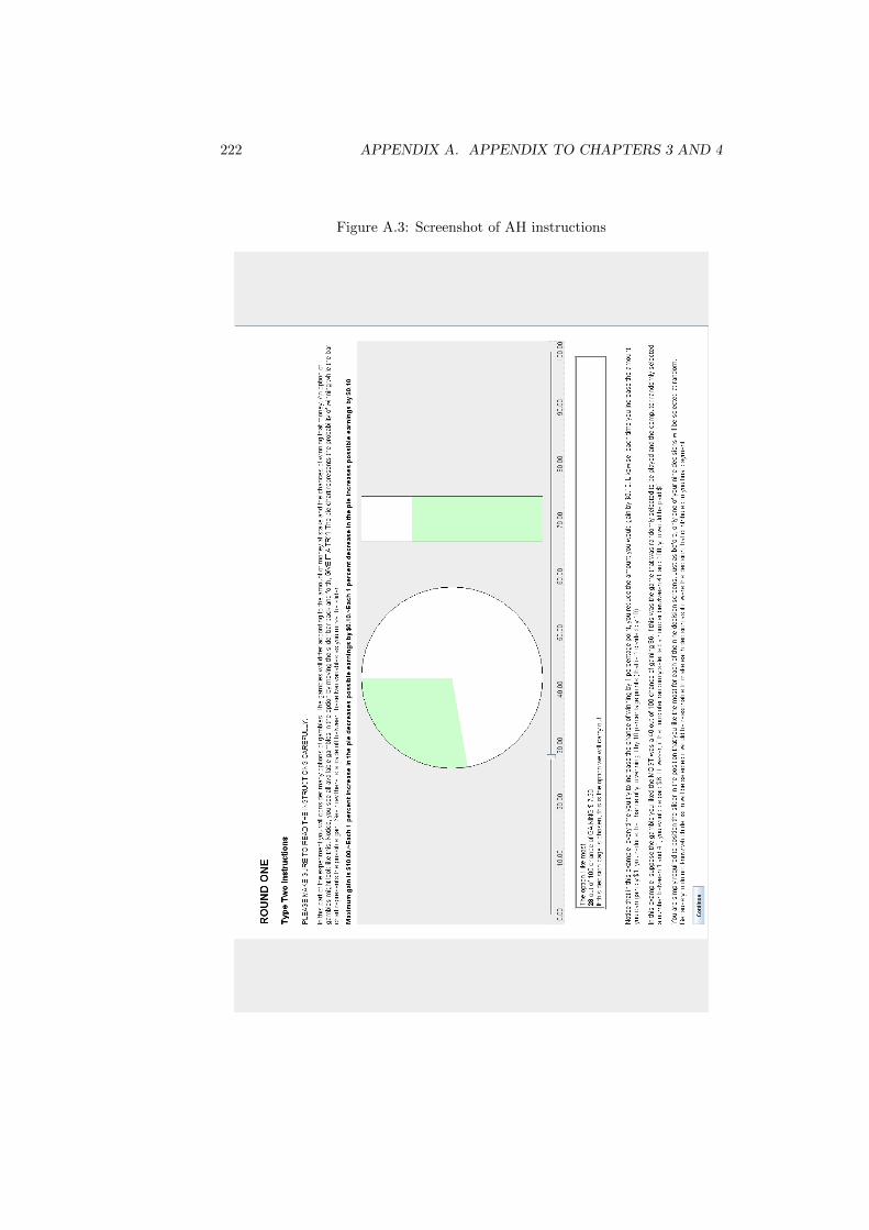
222 APPENDIX A. APPENDIX TO CHAPTERS 3 AND 4
Figure A.3: Screenshot of AH instructions

A.4. EXAMPLES OF EXPERIMENTAL SCREENS 223
Figure A.4: Screenshot from our experiment using HL

224 APPENDIX A. APPENDIX TO CHAPTERS 3 AND 4
Figure A.5: Screenshot from our experiment using AH

A.4. EXAMPLES OF EXPERIMENTAL SCREENS 225
Figure A.6: Screenshot from the film
Figure A.7: Pictures shown for option to save one of the two swimmers
(a) Save left swimmer (b) Save right swimmer

226 APPENDIX A. APPENDIX TO CHAPTERS 3 AND 4

Part V
Appendix to Part II
227


Appendix B
Appendix to chapter 7
229
230 APPENDIX B. APPENDIX TO CHAPTER 7
B.1 Experimental instructions
The following text presents the instructions provided to the experimental partic-
ipants. The text was read out to participants as described for the gift exchange
game. In case treatment sessions were used, the text in italics was included
additionally. For the second game, instructions were not read out, but partic-
ipants were made aware that the game structure had changed and that they
were asked to read through the instructions again.
B.1.1 Read out text
Dear participants,
Thank you for participating in our research project. This project investigates
the behaviour and choices of employers and workers in an experimental situ-
ation. The experimental design has been chosen so that it is similar to what
can be observed in real-world situation where an employer is hiring an employee.
During the experiment you will see a succession of different screens. There
are active screens and waiting screens. If you see a screen that asks you to
wait, please be patient, this means you are waiting for another participant to
make their decision. The experiment will continue immediately after the other
participants have made their decisions. This should only take a minute or two.
Now, please enter your participant number then click the ok button, which
is located in the lower right corner of your computer screen.
You will now see a screen with experiment instructions; please take the time to
go through them with me now.
Instructions:
You are about to begin the economic experiment. Before the experimental
session starts, please read the following instructions carefully. This is important
because the final payment you receive for participating in the experiment can be
B.1. EXPERIMENTAL INSTRUCTIONS 231
affected by how well you understand the instructions and your decisions during
the game.
Please note that all information provided during the experiment is treated con-
fidentially.
You are prohibited from communicating with other participants during the ex-
periment.
All the decisions you make during the game are anonymous. Neither other
participants nor the administrators can attribute decisions to any one individ-
ual.
If you have any questions now, or during this experiment, please indicate this
by raising your hand. Do not talk to other participants.
B.1.2 Gift exchange game
Game structure – part one
For the duration of the experiment you will be assigned the role of either an
employer or a worker. You will remain in this role for the whole experiment.
ıPlease be aware that in today’s session the roles of workers and employers
have been assigned such that the role of the workers is always assigned to a
foreign-born, or more specifically, an Asian-born person and the role of the em-
ployer is always assigned to an Australian-born person.
The experiment has 16 rounds. In each round, you will be randomly matched
with another player. That is, in every round a worker will be matched with a
new employer, or alternatively, an employer will be matched with a new worker.
The dollar values you see on the computer screens are ’experimental dollars’.
Your income and payoffs are calculated using these ’experimental dollars’. Your

232 APPENDIX B. APPENDIX TO CHAPTER 7
decisions, these calculations, and the four randomly chosen rounds for your final
payoff, determine how much you will receive for participating in the experiment.
The conversion rate from ’experimental dollars’ to the Australian dollars you
will receive for completing the experiment is:
100 experimental dollars = 5 Australian dollars.
Game structure – part two
As we mentioned before, the game has 16 rounds. Each round has three stages;
Stage 1: In the first stage the employer offers a worker a wage between 5
and 100 experimental dollars.
Stage 2: In the second stage the worker decides if she/he wants to accept
the employer’s wage offer.
If the worker does not accept the offer, the round ends and both the employer
and the worker are paid a fixed amount of 60 experimental dollars.
If the worker does accept the offer: the worker is paid the offered wage, and the
worker incurs a fixed cost of 6 experimental dollars.
Stage 3: The worker must then choose the level of effort he/she is willing
to put into the job. The level of chosen effort can be between 1 and 10. It
is this level of effort that determines the employer’s profit. Every additional
unit of effort costs the worker 4 experimental dollars and provides a profit of 20
experimental dollars to the employer.
To summarise what happens if the wage offer is accepted by the worker. The
income for the round will be:
For the employer: 50 - wage + 20* effort
B.1. EXPERIMENTAL INSTRUCTIONS 233
For the worker: 50 + wage - 4 * effort - 6
Throughout the experiment, use the scenario calculator on the right of your
screen to calculate the different outcomes. Now let’s do some test questions so
you can learn how to play the game and use the calculator.
B.1.3 Wage promising game
We play a different game for the remaining 8 rounds; each round is divided into
four stages.
Stage 1: In the first stage the employer offers a worker a wage between 5
and 100 experimental dollars.
Stage 2: In the second stage the worker decides if she/he wants to accept
the employer’s wage offer.
If the worker does not accept the offer, the round ends and both the em-
ployer and the worker are paid a fixed amount of 60 experimental dollars.
If the worker does accept the offer: the worker is paid the offered wage, and;
the worker incurs a fixed cost of 6 experimental dollars.
Stage 3: The worker must then choose the level of effort they are willing
to put into the job. The level of chosen effort can be between 1 and 10. It
is this level of effort that determines the employer’s profit. Every additional
unit of effort costs the worker 4 experimental dollars and provides a profit of 20
experimental dollars to the employer.
Stage 4: In the fourth stage the employer is informed about the level of effort
chosen by the worker. Depending upon what the employer thinks about the
level of effort chosen by the worker, the employer can change the wage they
offer to the employee. In this decision, the employer is not bound to the wage

234 APPENDIX B. APPENDIX TO CHAPTER 7
offer made in stage 1. The employer decides the final wage he will pay the
worker by choosing a wage between 5 and 100 experimental dollars.
To summarise what happens if the wage offer is accepted by the worker. The
income for the round will be:
For the employer: 50 - wage + 20* effort
For the worker: 50 + wage - 4 * effort - 6

B.2. EXPERIMENTAL SELECTION 235
B.2 Selection into the experiment and potentialinfluence on experimental results
The study was designed to select students into the laboratory who were suitable
for studying the interaction between Australians and Asians. However, the
questionnaire also allowed to investigate potential selection into the experiment
of students that responded to the questionnaire.1 For this, 3 steps of selecting in
or out of experiments can be considered. The first was a question included in the
questionnaire, asking students if they would generally be willing to be included
in an experimental database, from which invitations to experiments would be
send. In order to be included in the database students had to provide a readable
and correct email address. Furthermore, an opt-out question was included that
the students were able to tick if they were not interested in participating in any
experiment. Based on these two criteria, potential participants were included
into the database. This served as the first selection mechanism; however, the
selection at this stage was not strong, as 84% of the questionnaire respondents
were included into the database.
The second step was done by the experimenters, only selecting students that
were in the required cultural groups and had answered the language proficiency
question correctly. This was the second, and desired selection effect. In a third
step participants were then able to register for experiments and come to the
laboratory.2 In case they did so, they were recorded as having participated in
the experiment; this also included participants that had to be sent home due
to overbooking or under-booking after paying them a show-up fee. Here the
selection was much stronger, as only 7% of all respondents and 9% of those
included in the database came to the laboratory for an experiment.
1As the questionnaires were handed out early in the semester and in all of the main lectures,a very large fraction of the students could be approached; furthermore, once asked to fillout the questionnaire, a large majority filled out the questionnaire (although this was notcompulsory), and only very few students decided not to look at the questionnaire or returnedblank copies.
2The set of students being considered as having participated was extended to those thatcame to a second experimental study, which drew on the same subject pool, but for whichalso students in the non-Australian and non-Asian groups were invited. Extending this setdoes, however, not lead to any changes in the selection pattern observed.

236 APPENDIX B. APPENDIX TO CHAPTER 7
B.2.1 Selection into the experimental database
To find out about the selection into the database, it was studied if any of
the data collected in the questionnaire determined whether participants were
inserted into the database. As these were of particular interest for this study,
the relationship between trust measures on the selection was investigated more
closely. Table B.1 reports the results of these (OLS) estimations, considering the
influence of the trust variables and further demographics and attitudes collected
in the questionnaire.3 As this study was aimed at investigating the decisions
and interaction between the two largest cultural groups in the sample, results
are shown for Australians and Asians separately. As can be seen in table B.1,
there were some trust variables that had a statistically significant influence
on the decisions of questionnaire respondents to be included in the database.
However, the economic importance of the selection was small, as accounting
for only around 1-2% of the variance for Australians and only being somewhat
higher for Asians.
To get a better understanding of the importance of any of these singular fac-
tors for the selection into the experiment, an iterative procedure of successively
eliminating insignificant variables was used to identify what might have been
driving the selection. Table B.2 shows regression results, which emerged out of
this iterative procedure. As can be seen, there are a number of variables from
the questionnaire that had a statistically significant influence on whether some-
one was included into the database or not. However, the economic significance
of these variables is again very low, as even jointly only accounting for a very
small fraction of the variance.
As can be seen in the table, factors driving selection are different between
the groups and the selection effect is larger for Asians than for Australians.
The main variable driving this result is language ability, which might indicate
that comprehension might play a role determining whether an individual was
included. However, this is not necessarily undesirable, as those Asians finally
migrating to Australia will be more likely those with somewhat better language
abilities, since this is one of the main criteria which have to be met when ap-
3Marginal effects on Probit regression that were used as an alternative provide with qual-itatively very similar results.
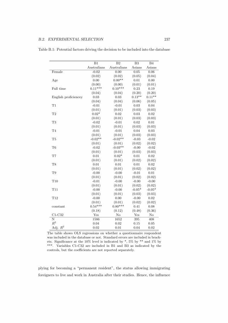
B.2. EXPERIMENTAL SELECTION 237
Table B.1: Potential factors driving the decision to be included into the database
B1 B2 B3 B4Australians Australians Asians Asians
Female -0.02 0.00 0.05 0.06(0.02) (0.02) (0.05) (0.04)
Age 0.00 0.00** 0.01 0.00(0.00) (0.00) (0.01) (0.01)
Full time 0.11*** 0.10*** 0.23 0.19(0.04) (0.04) (0.20) (0.20)
English proficiencey 0.03 0.03 0.13** 0.11**(0.04) (0.04) (0.06) (0.05)
T1 -0.01 -0.01 0.03 0.04(0.01) (0.01) (0.03) (0.03)
T2 0.02* 0.02 0.03 0.02(0.01) (0.01) (0.03) (0.03)
T3 -0.02 -0.01 0.02 0.01(0.01) (0.01) (0.03) (0.03)
T4 -0.01 -0.01 0.04 0.03(0.01) (0.01) (0.03) (0.03)
T5 -0.02** -0.02** -0.03 -0.02(0.01) (0.01) (0.02) (0.02)
T6 -0.02 -0.03** -0.00 -0.02(0.01) (0.01) (0.03) (0.03)
T7 0.01 0.02* 0.01 0.02(0.01) (0.01) (0.02) (0.02)
T8 0.01 0.01 0.01 0.02(0.01) (0.01) (0.02) (0.02)
T9 -0.00 -0.00 -0.01 0.01(0.01) (0.01) (0.02) (0.02)
T10 -0.01 -0.00 -0.00 -0.00(0.01) (0.01) (0.02) (0.02)
T11 -0.00 -0.00 -0.05* -0.05*(0.01) (0.01) (0.03) (0.03)
T12 -0.00 0.00 -0.00 0.02(0.01) (0.01) (0.02) (0.02)
constant 0.54*** 0.80*** 0.41 0.08(0.18) (0.12) (0.48) (0.36)
C1-C32 Yes No Yes No
N 1586 1652 395 408R2 0.04 0.02 0.15 0.05Adj. R2 0.02 0.01 0.04 0.02
The table shows OLS regressions on whether a questionnaire respondentwas included in the database or not. Standard errors are included in brack-ets. Significance at the 10% level is indicated by *, 5% by ** and 1% by***. Variables C1-C32 are included in B1 and B3 as indicated by thecontrols, but the coefficients are not reported separately.
plying for becoming a “permanent resident”, the status allowing immigrating
foreigners to live and work in Australia after their studies. Hence, the influence

238 APPENDIX B. APPENDIX TO CHAPTER 7
Table B.2: Potential factors driving the decision to be included into the databasein the full sample
B5 B6Australians Asians
Full time 0.08**(0.03)
English proficiencey 0.03 0.10**(0.04) (0.05)
T2 0.02*(0.01)
T5 -0.03***(0.01)
C13 -0.03**(0.01)
C18 0.01**(0.01)
C28 0.03***(0.01)
C10 -0.04*(0.02)
C21 -0.03**(0.02)
C3 -0.06**(0.03)
C31 -0.02*(0.01)
constant 0.68*** 1.10***(0.08) (0.10)
N 1701 433R2 0.02 0.07Adj. R2 0.02 0.06
The table shows pre-experimental questionnaire variables that drove theselection of subscription to the database. Standard errors are included inbrackets. Significance at the 10% level is indicated by *, 5% by ** and 1%by ***.
of the language questions represents some opting out before the experimenter-
induced selection strategy based on language proficiency that was employed for
this study.
B.2.2 Participation in the experiment
In a second step it was further investigated if, conditional on having subscribed
to the database, students came to the lab for participating in the experiment.
The selection on this second stage can similarly be analysed.4 Table B.3 shows
4Additional to the analysis shown in the tables, two other main specifications were consid-ered. One excluded the decision to subscribe to the database as a regressor; however, whilereducing the explanatory power of the regression, no qualitative difference in the results was

B.2. EXPERIMENTAL SELECTION 239
the results from (OLS) regressions analysis that looked at whether participants
came to the lab.5 As before, looking at the potential influence of the trusting
attitudes for the two different groups separately was the focus of this analysis.
There is no clear theoretical reason for trust to determine the decision to par-
ticipate. However, as trust was conjectured to influence experimental decisions,
trust was studied to understand the (external) validity of experimental results.
As can be seen in the estimation results reported in table B.3, some trusting
variables had a statistically significant influence on participation in an experi-
ment. This effect was weaker for Australians, for whom the total selection effect
into the experiment, even when considering the explicit selection criteria by the
participants (through their agreeing to be included into the database) and by
the experimenters (mainly through the language criterion) was very small. For
Asians, the selection effect was larger, again mainly being driven through lan-
guage ability, which was an explicit selection criterion to ensure comparable
comprehension of the participants of experimental instructions.
As some selection into the experiment was observable, again an iterative
procedure eliminating statistically non-significant regressors was used to inves-
tigate which factors were potentially driving the selection process. Table B.4
reports the outcome of this procedure. As can be seen in table B.4 there is some
statistically significant selection into the experiment observable, with some of
the trust and other attitudinal variables playing a role. However, the economic
significance of the selection effect is very small and is further reduced when not
including the explicit selection criterion of language ability.
However, the results in table B.4 also suggest that there is a bigger selection
effect for Asian then for Australian participants. Again, this effect is to a large
degree driven by the language proficiency requirement; but even when eliminat-
ing the language criterion and inclusion into the database, the selection effect is
stronger than for Australians. The three most influential variables are whether
individuals kept up a different social identity compared to their private identity
(C18), if they were religious (C21) and if they were favouring a hierarchical com-
evident as a result of this. The other analysis also recorded all participants that attended tothis (and) or a second study for which all students (hence also the non-Australian and non-Asian) were invited, which increases the number of individuals that decided to participate inexperiments. Again, there was no qualitative difference in the results when doing so.
5Again, marginal effects of Probit regressions provide with the same result.

240 APPENDIX B. APPENDIX TO CHAPTER 7
Table B.3: Potential determinants of participation in experimental sessions
B7 B8 B9 B10Australians Australians Asians Asians
In database 0.08*** 0.08*** 0.08** 0.11***(0.02) (0.02) (0.04) (0.03)
Female -0.00 -0.01 -0.04 -0.03(0.01) (0.01) (0.03) (0.03)
Age -0.00 -0.00 -0.00 -0.00(0.00) (0.00) (0.00) (0.00)
Full time 0.05* 0.05* 0.02 0.01(0.03) (0.03) (0.14) (0.14)
English proficiencey 0.06* 0.06* 0.06 0.06(0.03) (0.03) (0.04) (0.04)
T1 -0.01 -0.01* -0.00 0.00(0.01) (0.01) (0.02) (0.02)
T2 -0.01 -0.01 -0.03 -0.03(0.01) (0.01) (0.02) (0.02)
T3 0.02** 0.02* 0.00 0.00(0.01) (0.01) (0.02) (0.02)
T4 0.00 0.01 -0.02 -0.03(0.01) (0.01) (0.02) (0.02)
T5 0.00 0.00 -0.02 -0.01(0.01) (0.01) (0.02) (0.02)
T6 -0.00 -0.00 -0.01 -0.00(0.01) (0.01) (0.02) (0.02)
T7 0.01 0.01 0.02 0.03*(0.01) (0.01) (0.02) (0.02)
T8 -0.00 -0.00 0.00 -0.01(0.01) (0.01) (0.02) (0.02)
T9 -0.00 -0.00 -0.01 -0.01(0.01) (0.01) (0.02) (0.01)
T10 -0.01 -0.01 -0.03 -0.03*(0.01) (0.01) (0.02) (0.02)
T11 -0.00 0.00 -0.03 -0.02(0.01) (0.01) (0.02) (0.02)
T12 0.01 0.01 0.04** 0.04***(0.01) (0.01) (0.02) (0.02)
constant -0.13 -0.09 0.14 0.19(0.13) (0.09) (0.34) (0.25)
C1-C32 Yes No Yes No
N 1586 1652 395 408R2 0.05 0.02 0.21 0.13Adj. R2 0.02 0.01 0.10 0.09
The table shows OLS regressions on whether a questionnaire respondentcame to an experiment. Significance at the 10% level is indicated by *,5% by ** and 1% by ***. Variables C1-C32 are included in B7 and B9 asindicated by the controls, but the coefficients are not reported separately.
pany structure (C26). None of these variables has a direct intuition for why it
should change decisions in the experiment in a certain direction. Nevertheless,

B.2. EXPERIMENTAL SELECTION 241
Table B.4: Potential factors driving the decision of participation in experimentalsessions
B11 B12Australians Asians
In database 0.08*** 0.10***(0.02) (0.03)
Full time 0.06**(0.03)
English proficiencey 0.06** 0.07**(0.03) (0.04)
T3 0.02**(0.01)
C20 0.02**(0.01)
C22 -0.02***(0.01)
C23 -0.01*(0.01)
C28 0.02**(0.01)
C18 -0.02**(0.01)
C21 -0.02*(0.01)
C26 0.04**(0.02)
constant -0.15** -0.03(0.07) (0.08)
N 1703 434R2 0.03 0.07Adj. R2 0.03 0.06
The table shows pre-experimental questionnaire variables that drove the se-lection into the experiment separated for Australians and Asians. Standarderrors are included in brackets. Significance at the 10% level is indicatedby *, 5% by ** and 1% by ***.
these variables, as well as all others that showed some influence on selection
behaviour into the experiment, were considered when looking at the connection
between attitudes recorded in the questionnaire and experimental decisions.
B.2.3 Questionnaire variables and experimental decisions
In order to understand the importance of the selection effect into the experiment,
it was finally looked at the potential influence of attitudes recorded in the pre-
experimental questionnaire and experimental decisions. In this analysis the
experimental decisions were thought not to be influenced by the answers in the
pre-experimental questionnaire in the sense of “priming” respondents to make

242 APPENDIX B. APPENDIX TO CHAPTER 7
certain (e.g. more trusting or trustworthy) decisions. The reason for this was
that the questionnaire answers and experimental decisions were usually several
weeks and often even months apart from another. Nevertheless, they might
well be connected as both reflect general attitudes of the experimental decision
makers.
One first aspect is if trusting attitudes based on the questionnaire were giving
a similar result to what was inferred from experimental decisions. Secondly, it
is also interesting to investigate the influence of the other variables that had a
significant impact in the selection process as described in the section above.
In order to understand the influence of the variables, (OLS) regressions of
employer and worker decisions were used to understand the effect on decisions.
Furthermore, it was considered that general attitudes would have their strongest
impact in the first period of the two games, and that attitudinal variables would
have a comparatively minor impact compared to any game dynamics.6 In order
to identify these relationships, various specifications were used, which gave a
generally very mixed picture about the influence of the variables: It can be found
that general trusting attitudes using a combined measure of the 12 trusting
questions from the pre-experimental questionnaire was insignificantly related to
decisions over wage offers, efforts and final wages in the two games. This was
observable for first period decisions of the games, where game dynamics had
not yet influenced experimental decision patterns and general attitudes might
therefore show their strongest results.
Once each of the 12 different variables was included, however, a significant
relationship between some of the variables and experimental decisions could be
observed. A variable that seemed to play a significant role in wage offers was
T3, indicating that the more individuals thought others were honest, the lower
the wage offers were they made. This could for example in the WPG reflect
guilt aversion by the decision makers. Similarly, it was possible to observe if
some variables played a role when employers were interacting with Australians or
Asians. For example, variable T1, hence if it was reported to be rather careful in
interaction with strangers, led to lower wage offers when Australians interacted
6This would be suggested considering fixed effect model regressions of the experimentaldecisions, which provided with very similar results to those reported in the main section ofthe analysis.

B.2. EXPERIMENTAL SELECTION 243
with Asians, while it was not significant when interacting with Australians.
Hence those that reported to trust strangers less also showed less trust in the
GEG when playing with Asians.
However, the picture on basically all variables was mixed in the sense that
significance levels of the influence of questionnaire variables on experimental
decisions were usually low, i.e. mostly at a 5% or 10% level, differed for the
decision variables and were often sensitive to changes in the specifications or
not the same for the two different treatments of having a pure Australian or
Australian-Asian intercultural group (at the same time no significant treatment
and variable interaction effects could clearly be determined). Furthermore, it
was theoretically not clear why some of the trust variables should have a sig-
nificant influence while others would not, making it difficult to say if a causal
relationship between the variables exists, or if statistical factors drive the result.
In any case the economic significance of any relationship would be medium to
small, for example judging by the adjusted R2, which was below 15% for all
specifications and between 5% and 10% even when including all trusting vari-
ables jointly.7 This would correspond to less then half of the influence that
direct decision variables had (like the effort for final wage decisions) and all
trusting variables jointly explain less then adaptation behaviour in the course
of the game (as could be reflected using lagged variables).
The second and other interesting question was how the (non-intended) se-
lection into the experiment as described in the previous section might have
influenced decisions in some way. To do so, the relationship between the vari-
ables that had been significant for the two groups were related to the decisions
made in the experiment. Again, however, the results from this were not con-
clusive in the sense of directly pointing to any clear bias in decision patterns.
However, some of the variables were significantly related to decisions in the ex-
periments and were therefore investigated further. Results described here are
all referring to analysis of all periods of a game, as here results were generally
the strongest.8 As the variables having led to selection into the experiment
7Regression results are not presented here as it would be arbitrary to chose any out of thelarge multitude of specifications used.
8As before also the first period of each game was investigated separately, but as in thesealternative specifications the selection variables were usually all insignificant, no further em-phasis is put on this aspect here.
244 APPENDIX B. APPENDIX TO CHAPTER 7
were different between the two groups, Asians and Australians were analysed
separately.
The only variable that had been one of the selection variables into the ex-
periment and had a significant influence on decisions, was on C18 for Asians.9
Together, the selection effect and the effect on experimental decision might have
led to somewhat higher efforts by Asians. However, considering the joint selec-
tion and experimental effect, the economic significance of this variable was only
about 1%. The consideration that slightly lower effort level of Asians would
make them even more similar to Australians in the worker role further sup-
ports the conclusion of the main analysis, arguing for the similarity between
the decisions of the two groups. Hence, this selection effect does not change the
conclusion included in the main section.
For most decision patterns of employers a similar conclusion holds; hence,
there may be some selection, but it does no seem to have a strong influence
on the overall conclusion about the results of the experiment. The only critical
variable might be T3, which has an influence on selection into the experiment
and was significantly related to wage offers made.10 The relationship was such
that individuals who think people are more honest make lower wage offers.
This is somewhat against intuition, as it would indicate that decision makers
that trust less in others make higher wage offers, hence display higher trusting
levels. However, as the statistical and also the economic size of a selection
effect was considerable, the influence of this variable was further investigated.
Furthermore, the effect of the variable was not necessarily in the same direction
for interaction in homogeneous Australian and heterogeneous Australian-Asian
groups, although there was no statistical difference between the two groups when
testing for this in regressions using interaction effects. Table B.5 illustrates this
difference in significance as well as the insignificance of the difference when
looking at interaction terms.
Hence, any results underpinning the similarity between the two groups and
9This question asked if participants were behaving the same at work and at home. Thereis no clear causal intuition why this variable should drive decisions to influence decisions inthe experiment in one direction.
10The question asked “Most people answer questions honestly”. Hence, there is also somepotential causal relation additional to the statistical relationship between T3 and wage offers.However, although the considerations in the paragraph take it as if there was a true relation-ship, it should still be take in to account that the statistical significance of the effect mightbe driven by spurious effects (mainly through a type I error).

B.2. EXPERIMENTAL SELECTION 245
Tab
leB
.5:
Rel
atio
nsh
ipb
etw
een
wag
eoff
ers
an
dva
riab
les
ind
icati
ng
ase
lect
ion
effec
tin
toth
eex
per
imen
t
Gif
tex
change
gam
eW
age
pro
mis
ing
gam
eIn
terc
ult
ura
lA
ust
ralian
Join
tIn
terc
ult
ura
lA
ust
ralian
Join
tgro
up
gro
up
sam
ple
gro
up
gro
up
sam
ple
Eff
ortlag
5.6
5***
5.0
5***
5.3
8***
3.4
2***
2.6
6***
3.1
0***
(0.6
2)
(0.8
5)
(0.5
1)
(0.5
9)
(0.6
7)
(0.4
4)
T3
-3.9
4*
-3.7
9-4
.14*
-6.5
1*
-0.8
0-6
.81*
(2.3
3)
(2.8
5)
(2.4
1)
(3.3
7)
(2.9
8)
(3.4
4)
C20
-2.6
0-1
2.2
0**
-2.5
4-6
.36***
1.0
5-6
.55***
(1.7
9)
(5.0
2)
(1.8
2)
(2.2
4)
(5.3
6)
(2.2
9)
C22
-0.8
3-4
.04
-0.7
4-4
.07
-4.7
3*
-4.2
1(2
.27)
(2.8
9)
(2.3
0)
(3.5
4)
(2.3
5)
(3.5
6)
C23
-2.9
3-0
.86
-2.8
4-4
.08
-7.0
7*
-4.1
9(2
.82)
(3.7
5)
(2.8
4)
(2.9
5)
(3.7
7)
(2.9
9)
C28
0.2
7-1
.90
0.3
3-0
.90
2.5
2-0
.82
(2.6
0)
(4.0
2)
(2.6
5)
(3.8
0)
(4.7
9)
(3.8
3)
Inte
rcult
ura
lgro
up
26.0
5-3
9.1
3(2
8.1
0)
(31.9
8)
(Inte
rcult
ura
lgro
up)*
T3
0.5
56.1
9(3
.64)
(4.3
6)
(Inte
rcult
ura
lgro
up)*
C20
-9.1
7*
7.7
6(4
.93)
(5.3
6)
(Inte
rcult
ura
lgro
up)*
C22
-3.2
0-0
.21
(3.6
2)
(4.2
0)
Inte
rcult
ura
lgro
up)*
C23
2.1
1-2
.76
(4.5
9)
(4.7
2)
(Inte
rcult
ura
lgro
up)*
C28
-2.1
33.2
9(4
.68)
(5.8
5)
const
ant
72.4
1***
102.7
3***
72.8
8***
126.7
3***
95.8
2***
130.3
4***
(21.2
3)
(17.3
5)
(21.6
5)
(24.8
2)
(19.1
1)
(25.9
9)
N266
217
483
304
248
552
R2
0.3
60.3
40.3
50.4
00.2
70.3
5
The
table
show
sth
ere
lati
onsh
ipb
etw
een
wage
off
ers
and
vari
able
sfr
om
the
pre
-exp
erim
enta
lques
tionnair
e,w
hic
hhad
asi
gnifi
cant
influen
ceon
part
icip
ati
on
inth
eex
per
imen
t.Sta
ndard
erro
rs(c
lust
ered
by
indiv
idual)
are
incl
uded
inbra
cket
s.Sig
nifi
cance
at
the
10%
level
isin
dic
ate
dby
*,
5%
by
**
and
1%
by
***.

246 APPENDIX B. APPENDIX TO CHAPTER 7
documenting relatively similar interaction between the groups would be further
supported if the selection effect is taken in to account: Not being subject to the
selection effect would make wage offers to Asians and Australians even more
similar to one another.
The only critical point remaining is hence the different interaction between
Australians and Asians in the final wage decision of the WPG. Here, there would
be two potential effects through the selection reflected in the variable T3 as illus-
trated in table B.6.11 The effect is that it would slightly reduce the higher reward
of effort when interacting with Asians; however, even when this effect of higher
rewarding effort of Asians is somewhat reduced, the statistical significance of
the difference should still remain. The other effect would be a higher willingness
to pay Australian workers based on the previous wage promise. This would in
turn further strengthen the point of difference in the role that received effort
and previous wage promises play in the interaction between the two groups.
Hence, the overall conclusions in the main analysis should remain as it is, even
when a potential selection effect of students into the experiment is taken into
account.
11The following argument is motivated by several tests using interaction effects in regressionsof the data which are – due to their multitude – not documented here.

B.2. EXPERIMENTAL SELECTION 247
Table B.6: Relationship between final wages in the WPG and variables indicat-ing a selection effect into the experiment
Intercultural Australian Jointgroup group sample
Effort 5.64*** 8.41*** 6.93***(1.00) (0.78) (0.69)
T3 -6.21 7.36 -5.20(4.47) (4.39) (4.39)
C20 -0.07 0.55 0.52(3.29) (6.72) (3.45)
C22 2.15 -5.74 2.68(3.75) (3.85) (3.69)
C23 2.08 2.45 2.03(4.28) (4.34) (4.21)
C28 -0.44 13.75** -0.83(5.27) (5.24) (5.22)
Intercultural group -61.43(47.70)
(Intercultural group)*T3 12.20*(6.18)
(Intercultural group)*C20 -0.19(7.66)
(Intercultural group)*C22 -9.46*(5.47)
(Intercultural group)*C23 0.62(6.07)
(Intercultural group)*C28 15.06**(7.54)
constant 24.09 -63.79* 10.40(35.72) (34.38) (34.16)
N 240 205 445R2 0.28 0.50 0.38
The table shows the relationship between final wages and variables fromthe pre-experimental questionnaire, which had a significant influence onparticipation in the experiment. Standard errors (clustered by individual)are included in brackets. Significance at the 10% level is indicated by *,5% by ** and 1% by ***.

248 APPENDIX B. APPENDIX TO CHAPTER 7
B.3 Decisions of double participants
As described in the procedures section, a total of 9 participants came to the
laboratory twice. However, there was no clear indication that including or
excluding the second participation of these double participants changed the
overall results reported in the main text. However, it was further investigated
if participants changed their behaviour between the two sessions. The following
paragraphs describe decisions of these individuals over the two participations.
Following this analysis it is further discussed if including the participants twice
in the analysis is adequate.
However, for some of the double participants decisions over the two par-
ticipations were not directly comparable, for example because they played in
the role of the worker in the first participation and in the role of the employer
in the second participation. Furthermore, some subjects participated in both
homogeneous (Australian only) and heterogeneous (Australian-Asian) sessions.
Nevertheless, some comparisons between the sessions can be made. While it
does not appear that decisions were outside of the distribution of decisions of
all participants, it is nevertheless interesting to investigate if levels of reciprocity
or decision patterns might have changed between the first and the second par-
ticipation. This was tested for all participants for which such a comparison was
possible. However, all analysis included here should be interpreted with some
care, as only very small samples of 1-3 participants of a type of double partici-
pants served as the basis for comparison. The following sections describe these
comparisons for each type.
B.3.1 Employers in both games
Over the two experiments, 3 participants were employers in the first and the
second experiment. One of them was twice an employer in an Australian session
and the other two first in an Australian and second in an Australian-Asian
session. In order to test if there might be a change in behaviour observable
between the two rounds, a t-test for the levels of wage offers and final wages
in the two games were used. Firstly, decisions of those participants that were
first employers in a homogeneous group and then in a heterogeneous group
were studied. The results from these tests show that wage offers in the second

B.3. DECISIONS OF DOUBLE PARTICIPANTS 249
participation were significantly higher at a level of 10% in the GEG and at the
level of 1% in the WPG over all rounds of the games. However, final wages in
the WPG were not significantly higher in the second participation. Figure B.1
illustrates this finding.
However, it has to be recognised that these decisions were potentially condi-
tional on previous decisions over the rounds. Indeed, when just looking at the
first period of the game, there was no significant difference between the first and
the second participation. Hence, looking at regressions that use the previous
period as controls, only higher wage offers in the WPG remain significant when
controlling for decisions in previous periods. This can be interpreted such that
participants had gained a better understanding of the game dynamics. The
cheap talk character of the wage offer was potentially better understood, and
the positive effect of making higher offers might have been learned from the first
participation to the second.
Another interpretation of the result could be that reverse discrimination to-
wards Asians is observable. Therefore, the decisions of those double participants
first in an Australian and then in an Australian-Asian group were compared to
the individual that had been an employer in two mixed Australian-Asian ses-
sions. This individual displayed a similar pattern. In the second participation
wage offers in both games as well as final wages were higher, whereas the differ-
ence was only significant for the wage offer in the WPG (at a 5% level). Figure
B.2 illustrates the decisions of this participant between the two periods. The
pattern was similar to the other individuals that had been employers in the
two different treatments. Hence, there is no indication that moving from the
Australian to the Asian group was responsible for the shift in this behaviour.
Instead, there seems to be a general increase in the willingness to reciprocate
when a participant came to the lab twice.
A question arising from this was if there was a lump-sum higher willing-
ness to reciprocate for those individuals that were invited twice, or if also the
pattern of interaction between the first and the second participation changed.
And, if so, the change in the pattern would not correspond to what could be un-
derstood as normal variation equally observable between two randomly chosen
experimental subjects. Looking at the data confirmed the conjecture that the

250 APPENDIX B. APPENDIX TO CHAPTER 7
Figure B.1: Decisions of employers which were first in a homogeneous and secondin a heterogeneous session
(a)
40
50
60
70
80
90
First participation Second participation
Wa
ge
off
er
Graphs by doublesecond
(b)
40
50
60
70
80
90
First participation Second participation
Wa
ge
off
er
(c)
02
04
06
08
01
00
First participation Second participation
Fin
al w
ag
e
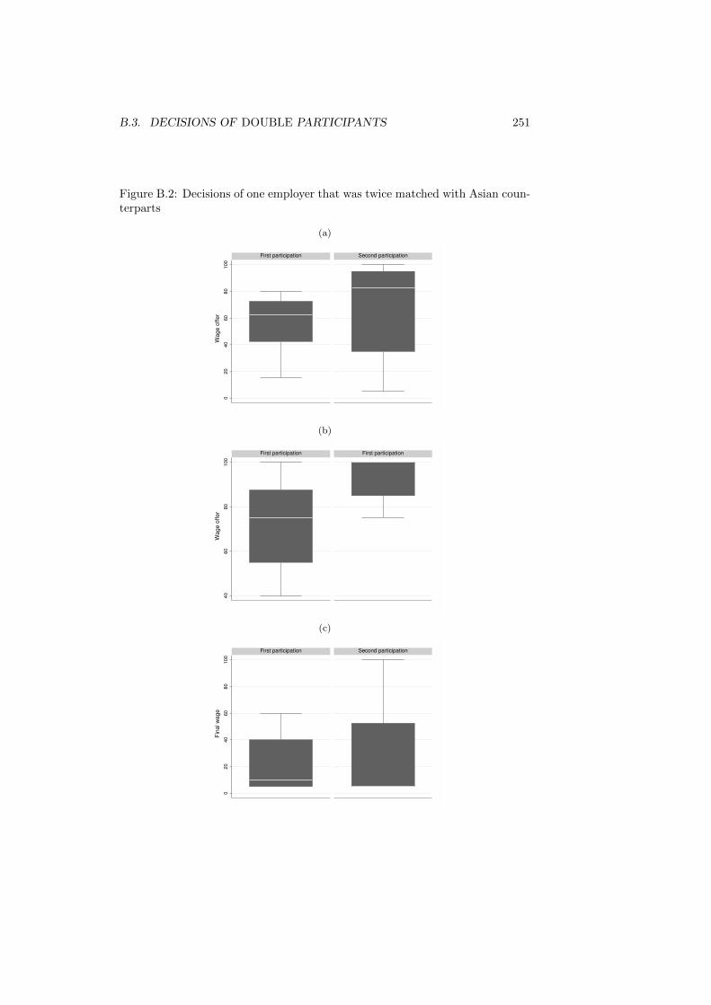
B.3. DECISIONS OF DOUBLE PARTICIPANTS 251
Figure B.2: Decisions of one employer that was twice matched with Asian coun-terparts
(a)0
20
40
60
80
10
0
First participation Second participation
Wa
ge
off
er
(b)
40
60
80
10
0
First participation First participation
Wa
ge
off
er
(c)
02
04
06
08
01
00
First participation Second participation
Fin
al w
ag
e

252 APPENDIX B. APPENDIX TO CHAPTER 7
reaction patterns for the first and the second participation were similar. That is,
there was some variation in within-individual decisions, but this pattern did not
shift decisions in a specific direction and was not necessarily unrepresentative
of normal decision patterns.
B.3.2 Workers in both games
Of the participants that came to the laboratory twice, some were twice in the
worker role. Of these 3 were Asian participants. To analyse their decisions
t-tests over all periods were used to understand if decisions changed between
the two participations. These tests showed insignificantly higher efforts in the
GEG and in the WPG significantly lower efforts at the 1% level. Figure B.3
illustrates this observation.
However, it has to be taken into account that efforts are always conditional
decisions and therefore the higher efforts might stem from higher wage offers or
more reciprocal reaction patterns between the sessions. Indeed, if such reciprocal
relationships are taken into account, the significant effect disappears.12 Table
B.7 illustrates this effect for the 3 Asian participants that were in the worker
role twice. Hence, there is no clear systematic change observable. However, any
tendency could be similar to what was observable for double participants in the
employer role, indicating higher general reciprocity in the second participation
and a better understanding of the cheap talk characteristic of wage offers in the
WPG.
B.3.3 Varying employer-worker roles
There were also participants that had the worker role during their first participa-
tion in an Australian group and the employer role in their second participation
in an Australian-Asian group. Evidently, it is difficult to determine if there is
any change in decisions between the two participations, as the role taken differs
between the two participations. One potential check is, however, to test if wage
offers and final wages in the second participation are higher then in the first
one. This would indicate that ex-workers treat current workers differently than
they were treated themselves. T-tests for the two participants who were first
12See the main section for variables potentially having an influence on decisions.
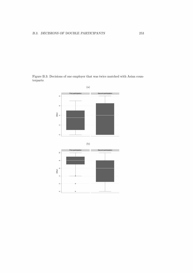
B.3. DECISIONS OF DOUBLE PARTICIPANTS 253
Figure B.3: Decisions of one employer that was twice matched with Asian coun-terparts
(a)
02
46
8
First participation Second participation
Eff
ort
(b)
02
46
81
0
First participation Second participation
Effo
rt

254 APPENDIX B. APPENDIX TO CHAPTER 7
Table B.7: Effort decisions of Asian workers
GEG WPG WPG—2nd participation 0.45 -2.36 -1.55
(0.77) (1.42) (1.39)Wage offer 0.08*** 0.05 0.03
(0.01) (0.03) (0.03)Final waget−1 0.04
(0.02)N 48 48 43R2 0.69 0.22 0.33
The table illustrates OLS regressions of effort decisions ofAsian participants twice in the worker role. Standard er-rors (clustered by individuals) are included in brackets. *signifies significance at the 10% level, ** a the 5% level and*** at the 1% level.
employers and then workers showed that they offered significantly higher wages
in both games and paid higher final wages. Furthermore, in the WPG wage
offers were even always the highest promise of 100. Figure B.4 illustrates these
relationships for the two participants.
However, again potential reciprocal relationships over the periods have to be
taken into account. For example, if in the first round a higher offer is made, this
is likely to lead to higher effort by the worker and through this induces higher
wage offers by the employer in the following periods (this mechanism works
although employers are not repeatedly interacting with workers); furthermore,
in the WPG final wages are potentially dependent on effort, which is influenced
by the wage offer. Indeed, once controlling for these reciprocal relationships
the significance of differences vanishes, except for wage offers in the WPG,
which again might reflect learning about the strategic meaning of the final wage
variable and the fact that it is not binding.
B.3.4 Adequacy of including repeated participants twicein the analysis
As described above, there were some, but no major changes in decisions of
participant that repeatedly came to the experiment. The results indicated that
there was a (weak) tendency to be more reciprocal in the second experiment,
although this effect was not significant once controlling for dynamic patterns.
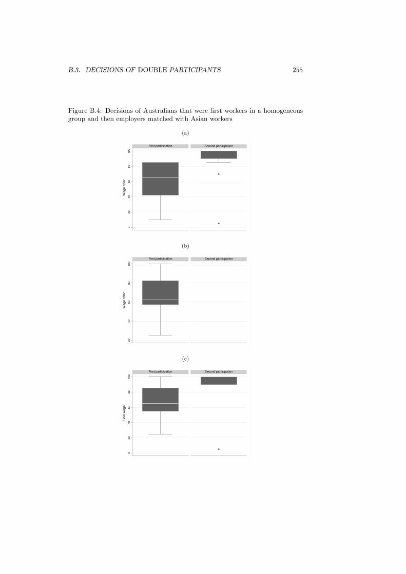
B.3. DECISIONS OF DOUBLE PARTICIPANTS 255
Figure B.4: Decisions of Australians that were first workers in a homogeneousgroup and then employers matched with Asian workers
(a)0
20
40
60
80
10
0
First participation Second participation
Wa
ge
off
er
(b)
20
40
60
80
10
0
First participation Second participation
Wa
ge
off
er
(c)
02
04
06
08
01
00
First participation Second participation
Fin
al w
ag
e
256 APPENDIX B. APPENDIX TO CHAPTER 7
However, potential differences are maybe too easily rejected, as for all types of
double participants there were only very small sub-samples, and it is not possible
to pool the data.
Nevertheless, it seems necessary to ask if including the participants twice
changes the outcomes of the results reported in the main part. For this two
main questions were asked. The first is if the double participants are not repre-
sentative of the other decision makers in the experiment. The second is if they
might have been driving some of the results described in the main section.
Regarding the first question, there does not seem to be any difference be-
tween individuals that came to the experiment twice using data from the pre-
experimental questionnaire. That is, these participants have similar demograph-
ics and attitudes compared to other participants. However, there was a be-
havioural change observable between participations. As could be seen in the
description above, during the second participation more reciprocity was observ-
able, both from the employer as well as from the worker side. But is this is a
level effect or did the pattern of interaction change for the double participants?
This question is difficult to answer given the sample sizes of the repeated deci-
sion makers. In order to scrutinise one can nevertheless consider if the reaction
patterns in the regression analysis change. Using regression results as described
above, it can be concluded that there was no indication that decision patterns
were significantly different for the double participants in either the first nor the
second participation compared to decision patterns of the other participants.
However, it should still be asked if even slight changes in decision patterns
could drive towards the results described in the main text. This is illustrated
by the fact that the double participants were always in Australian-Asian ses-
sions for their second participation. Given that reciprocity might be increasing
from the first to the second participation, this could give rise to a tendency of
the Australian-Asian sessions to show higher levels of reciprocity. While this
effect could be detected, it was insignificant. In any case, even with increased
statistical power a significant result would render the conclusion that the two
groups of Australians and Asians are similar in their decisions more strong. It
can therefore be concluded that including the double participants is adequate.

Appendix C
Appendix to chapter 8
257

258 APPENDIX C. APPENDIX TO CHAPTER 8
C.1 Experimental Instructions
The following is a translated version of the experimental instructions for the
case in which the gift exchange game was payed first and in which locals were in
the role of the employer and migrants in the role of the worker. The treatment
is included in italics (here, but not on the original screen). Screens 1-3 always
occurred in the order provided, while the game-specific screens were reversed
between sessions.
C.1.1 Screen 1
Please enter your participant number.
C.1.2 Screen 2
Instructions part 1:
This is an experiment of experimental economics. Please read the note be-
low before everything starts.
The note is very important, because your understanding of it and the choice
you make will affect the final result of the experiment.
All the information in this experiment will remain confidential.
During the experiment, you cannot talk to any other participants.
All the decisions and choices you make are made anonymously and no one will
know about the choice maker’s identity, be it other participants or the monitors
of this experiment.
Whenever you have any question, please raise your hand and do not communi-
cate with other participants.

C.1. EXPERIMENTAL INSTRUCTIONS 259
C.1.3 Screen 3
Instructions part 2:
In the current experiment, you will play a role as either employer or worker
and the role you play will stick to you throughout the whole experiment.
In todays game, the Nanjing locals will keep playing the role of employer, and
non Nanjing local will keep playing the role of worker.
There are 16 rounds in this experiment and in each round you will be ran-
domly regrouped with another participant.
More specifically, in each round, every worker will meet a new employer and
vice versa.
The amount of money shown on the computer screen is called experimental
dollars, your income and payment will be calculated by those experimental dol-
lars.
Your actual final reward will be affected by: 1. your decision, 2. the exchange
from experimental dollars into RMB, 3. your total income in the 4 round of
experiment randomly chosen by the computer.
The exchange rate between experimental dollar and RMB is:
100 dollars = 5RMB
C.1.4 Screen: Gift exchange game
The structure of the game
As is mentioned before, the experiment consists of 16 rounds of game. And
there are 3 stages in every round.

260 APPENDIX C. APPENDIX TO CHAPTER 8
Stage 1:
The employer will raise a salary proposal to the worker. The salary should
be between 5 to 100 dollars.
Stage 2:
The worker will decide whether to accept the proposal.
If the proposal is rejected by the worker, then the round ends. And both em-
ployer and worker get the same amount of income which is 60 experimental
dollars.
If the proposal is accepted, then the worker gets the salary in the proposal
and pays 6 dollars as a fixed cost of the work.
Stage 3:
In this stage, the worker will choose the level of effort they made in the work
from level 1 to level 10. The higher the level, the more efforts the worker makes.
The level of efforts will affect the income of the employer.
With 1 level increase in effort, the worker will bring 20 dollars income to the
employer while the worker himself needs to sacrifice 4 dollars for the effort he
makes.
Generally, if the worker accepts the proposal of the employer, the income of
both sides in this round should be:
For the employer:
50 - salary + 20 * the level of effort the worker chose to make in the work

C.1. EXPERIMENTAL INSTRUCTIONS 261
For the worker:
50 + salary - 4 * the level of effort the worker chose to make in the work -
6
C.1.5 Screen: Description of the wage promising game
In the last 8 rounds of game, the game will be a little bit different from previous
games. Each round of game will be divided into 4 stages.
Stage 1:
The employer will raise a salary proposal to the worker. The salary should
be between 5 to 100 dollars.
Stage 2:
The worker will decide whether to accept the proposal.
If the proposal is rejected by the worker, then the round ends. And both em-
ployer and worker get the same amount of income which is 60 experimental
dollars.
If the proposal is accepted, then the worker gets the salary in the proposal
and pays 6 dollars as a fixed cost of the work.
Stage 3:
In this stage, the worker will choose the level of effort they made in the work
from level 1 to level 10. The higher the level, the more efforts the worker makes.
The level of efforts will affect the income of the employer.

262 APPENDIX C. APPENDIX TO CHAPTER 8
With 1 level increase in effort, the worker will bring 20 dollars income to the
employer while the worker himself needs to sacrifice 4 dollars for the effort he
makes.
Stage 4:
The employer will be informed about the level of effort that the worker chooses.
The employer can change the amount of salary in the proposal according to
worker’s level of effort.
In other word, the employer does not have to pay the salary in the proposal
of stage one. He can readjust the amount of salary. The salary should be
between 5 to 100 dollars
C.1.6 Screen: Practice questions
In the experiment, please use the calculator on the right of the screen. Here is
a little practice which will help you understand the game and the calculator
Question 1
If the employer proposed a 50-dollar salary, and the worker chooses level 2 of
effort, then the income of both sides are:
Question 2
If the worker rejects the proposal:
Question 3
If the employer proposed a 100-dollar salary, and the worker chooses level 10 of
effort, then the income of both sides are:

C.2. RECRUITEMENT OF PARTICIPANTS 263
C.2 Recruitement of participants
The subjects we recruited were housekeepers, or household aids in Nanjing, the
provincial capital of Jiangsu, China, which had a population of around 7.7 mil-
lion (in 2009).1 Housekeeping services comprise activities like cleaning, cooking
or caring for elderly, children and pets. The housekeepers were, besides their
hukou status deemed to be comparable, particularly with respect to the distri-
bution of education, age and gender, making them suitable for an experimental
study. As most migrant housekeepers in our study came from rural places within
a distance of 5-6 hours drive from Nanjing and only few came from the inner or
western (hence further distant) regions, cultural differences between our groups
were relatively small. Focusing on this low-skill and low-income group also al-
lowed us to mitigate the problem that wealth and education (through higher
income) are the major ways to change status and obtain local hukou, resulting in
a potentially causal relationship between hukou status and income or education.
For the group of housekeeping subjects, status changes driven by income or ed-
ucation should be a negligible factor, which makes hukou status an exogenous
label for our participants.
We controlled for hukou status throughout the recruitement process of our
participants. However, status was not itself part of our advertisement. We hired
our participants on the regular labor market for housekeepers. Most house-
keepers are self-employed and (or) represented through working agencies. An
estimated number of over 1000 such agencies cover six urban districts as well
as the suburban area, each typically representing around 100 ayis. Ayis in turn
often seek employment through more than one channel, being represented by
more than one agent as well as searching for job opportunities privately in their
local community.
Making use of this infrastructure, we recruited participants using several
channels. We collected contact information online, used local newspapers and
1The housekeeping sector in Nanjing has a both local and migrant labor force. Historically,the housekeeping labor force was dominated by rural workers without local hukou. Sincethe late 1980s, more and more local workers joined the housekeeping service industry asstate-owned enterprises laid off low-skilled or abundant workers during institutional reform orprivatization. Among these unemployed workers, the low-skilled or aged women had difficultiesin getting hired again in privatized enterprise or other business companies. As a result, manyof these women stayed at home or worked as housekeepers.

264 APPENDIX C. APPENDIX TO CHAPTER 8
contact information on blackboards on which housekeepers advertised their ser-
vices.2 Using these sources, we contacted agencies via phone and made an
appointment with the agents if they agreed to. Some of the agencies doubted
about the credibility and security of the experiment and refused to offer their
help, probably afraid of leaking information on their ayis. To convince them we
tried to meet agents in person and had an interview with them.
During the recruitement process, we also became aware of over 100 ayis
taking training courses at a local trade college and made use of these partici-
pants as well. Those ayis had to take a paper exam and a practical exam on
housekeeping service before receiving their qualification certificate. This cer-
tificate is not a requirement for housekeepers, but can be of additional merit.
We were able to gather information about the hukou status of those ayis and
their educational background, which allowed us to assess the required level of
qualification. In order to use these helpers, we organized permission of the col-
lege to arrange experiments in the time between two exams. Once the helpers
finished the experiment, they could go ahead taking their practical exam on
housekeeping. Furthermore, before the experiment, we conducted a short inter-
view with candidates to further eliminate unqualified ayis. Participants were
also required to take a computer training test before entering into the test round
of the experiment, which facilitated the process of the experiment.
To avoid agencies with overlapping pools of housekeepers, we located agen-
cies that were far away from each other. We particularly made use of two
agencies from the Qing Huai and Xuan Wu districts that are at a 20 minutes
driving distance. The two agents committed to the recruitement of migrant
and local ayis for a commission fee of 10 Yuan for each qualified participant
with literacy or 5-6 years schooling. This is a comparable fee to what other
market participants pay for commissions. We asked agents to inform the can-
didate helpers of our requirement (i.e. literacy and information on their hukou
status; moreover, we excluded helpers below 18 years of age) as well as about
the payment opportunities. We guaranteed each participant a minimum pay-
ment for joining the experiment of 40 Yuan. Most of the ayis were motivated
2The websites we used for our online recruitement werehttp://nanjing.liebiao.com/jiazheng/ and http://www.zhongguoyuesao.com/. Helpfulnewpapers were Yangtze Evening Post and Modern Express; furthermore, some participantswere recruited using university Blackboards.

C.2. RECRUITEMENT OF PARTICIPANTS 265
to join the experiment by a possible payoff up to over 100 Yuan based on their
performance.
266 APPENDIX C. APPENDIX TO CHAPTER 8
C.3 Experimental data
The following section provides further information about the strategic meaning
of the decision variables and the distribution and structure of our experimental
data.
C.3.1 Strategic meaning of the variables
In both the gift exchange game and the wage promising game the first decision
variable in each period is the wage offer by employers. However, the strategic
importance of this offer is different between the two games. In the gift exchange
game, the offer is binding and tangible. Knowing this, together with the fact
that the incentive structure of the workers is such that no, or only minimal
efforts should be returned when workers maximize their own payoff, employers
should offer wages of less than 20 (these would be rejected) if they assume selfish
workers. Higher offers only make sense if employers believe that workers do not
only maximize their own payoff, but will share the mutual profit from higher
wages in such a way that higher wages are also beneficial for the employer. This
believe about a mutually beneficial response by the worker can be interpreted
as trust in the worker’s trustworthiness.
A large amount of the experimental literature indicates that participants
trust each other to some degree and would predict that employers chose wages in
the middle range, judging their experimental counterparts as having a medium
level of trustworthiness. As we chose the parameters for our payoff functions in
line with the literature, we would expect that we will also observe many decision
in the medium range. Our results generally confirm these predictions and even
show a higher willingness to trust workers. I.e., we find a surprisingly small
fraction of wage offers in the low and medium category (wage offers ≤ 70) and
a high fraction in the high and maximum category in the gift exchange game.
In the wage promising game the wage offer is not tangible as it does not
determine final payments. In a sense it is just cheap talk and consequently any
distribution of wage offers is equally reasonable, if workers interpret wage offers
in the wage promising game as meaningless. The picture changes, however, if
employers avoid lying about the final wages they are willing to pay (as results by
Gneezy, 2005, had indicated). I.e., deviations from the wage promise would be

C.3. EXPERIMENTAL DATA 267
(e.g. psychologically) costly and avoided by employers (also see Charness and
Dufwenberg, 2006, about guilt aversion). As a result wage offers could serve as
true signals to workers. The fact that wage offers in the wage promising game
follow a very similar distribution as in the gift exchange game points out to such
a relationship.
Worker efforts are the second decision variable in both games. In the gift ex-
change game the level of effort chosen is the back-transfer from the worker to the
employer and can be interpreted as the worker’s trustworthiness. The incentive
structure for effort levels is also clear: If wage offers are below 20, they should
always be rejected, as the outside option will be more valuable than accepting
and providing the lowest possible effort. All higher offers should be accepted
and the payoff-maximizing option is to return the minimum effort of one. How-
ever, if workers reciprocate more generous wage offers, they should respond to
higher wage offers with higher effort levels. This motivates the assumption that
any non-minimum efforts in the gift exchange game are conditional choices and
we observe this conditional relationship in our experiment.
In the wage promising game the strategic meaning of efforts is different. As
wage offers are not tangible, workers take the role of the trusting party when
choosing the level of effort and should only (accept and) choose high effort levels
believing that these will be reciprocated by employers. However, effort levels are
again not necessarily unconditional, if the wage offer by the employer in the first
stage is a signal containing true information. Indeed, if the (psychologically)
binding effect of wage promises is strong, we might even expect effort response
levels that are similar to the ones in the gift exchange game.
We find that these (conditional) relationships are true and that effort cho-
sen is very similar across games. That is, on average wage offers and efforts
are positively related. This positive reaction pattern is qualitatively true for
both games and also quantitatively surprisingly similar across games. Hence,
somewhat reflecting the distribution of wage offers in the first stage, efforts are
distributed such that there are many choices in the maximum range.3 While
there are only relatively few effort choices in the middle range, a second peak
3I.e., there is a noticeable fraction of rejections, which are recorded as an effort level of 0,a large number of minimum efforts and a high number of maximum efforts. This last aspectis particularly worth noticing as maximum efforts lead to an allocation of more than 1
2of the
mutual profit to the employer, which is not commonly observed in experiments.

268 APPENDIX C. APPENDIX TO CHAPTER 8
of efforts is in the rejection and minimum effort range. However, as efforts
are conditional choices, rejections and low efforts in many cases simply reflect
responses to low wage offers by employers.
In the wage promising game the final wage paid is the last decision variable.
For a profit-maximizing employer paying minimum wages, irrespective of the
efforts returned, is always the optimal strategy. However, this is not what is
observed; i.e. high levels of reciprocity can be found, as employers pay high (and
often maximum) wages, although on average employers return slightly lower
wages than promised in the first stage of the game and although the fraction
of minimum wages increases compared to the gift exchange game. However, as
final wage decisions are conditional on wage promises and returned effort, raw
figures should be interpreted with care.
C.3.2 Wage offers
Figure C.1 shows the distribution of wage offers in the two experimental games,
illustrating the large amount of high wage offers and the similarity of distribu-
tions accross games.
Figure C.1: Histograms of Wage offers
0.0
5.1
0 50 100 0 50 100
Wage promising game Gift exchange game
Density
Wage offerHistograms, by game
C.3.3 Efforts
Efforts chosen by workers are conditional variables; in the gift exchange game
wage offers lower than 25 should be rejected, leading to an effort of zero. For

C.3. EXPERIMENTAL DATA 269
higher wages the payoff-maximizing strategy is to provide minimum effort of
one. In the wage promising game all offers should be rejected if the workers do
not believe that these offers have any meaning. However, our results show that
relatively few offers are rejected, that there are few minimum efforts and that
there is a large number of maximum efforts. Figure C.2 illustrates this and also
shows that the distribution of efforts is very similar across games.
Figure C.2: Histograms of returned efforts
0.5
1
0 5 10 0 5 10
Wage promising game Gift exchange game
Density
EffortHistograms, by game
C.3.4 Final wages
Final wages can only be changed in the wage promising game. Figure C.3
provides a picture of the final wages paid by employers. It can be observed that
high levels of positive reciprocity are observable and that high wages are paid in
high fractions. However, the fraction of minimum wages increased between the
games and the fraction of high and maximum wages decreased. This indicates
that employers generally paid lower wages than they had promised. As the
decision over final wages might be conditional on effort levels provided by the
workers as well as on own wage offers in the first stage, these overview have to
be interpreted with care.
C.3.5 Interrelations
Throughout our analysis we assume that decision variables (wage offers, efforts
and final wages) influence each other. This conjecture is sustained when looking

270 APPENDIX C. APPENDIX TO CHAPTER 8
Figure C.3: Histogram of final wages
0.0
5.1
0 50 100 0 50 100
Wage promising game Gift exchange game
Density
Final wagesHistograms, by game
at average decisions taken by our experimental participants, as can be seen in
Figure C.4. As can be seen in Figure C.4a, on average higher wage offers
are answered by higher effort levels in both games. While the relationship is
not strictly increasing, a general relationship appears evident. Furthermore,
the relationship between wage offers and returned efforts appears to be very
similar for both games, indicating that workers interpret wage offers in the
wage promising game as quite meaningful - almost as if they were binding.
The relationship between effort levels provided in the wage promising game and
average final wages paid is shown in Figure C.4b.
Figure C.4: Simplified reaction patterns
(a) Relationship of efforts and wage offers
02
46
8
0 50 100 0 50 100
Wage promising game Gift exchange game
Average effort, by wage offer Fitted value line
Wage offer
(b) Relationship of final wages and efforts
40
50
60
70
80
0 2 4 6 8 10Effort
Final wage, by effort (PG) Fitted value line

C.3. EXPERIMENTAL DATA 271
C.3.6 Time effects
The experiment was designed such that all periods are independent and that
reputation effects through repeated interaction would not play a role. This
was done using random matching between experimental participants. Since
participants were informed about this matching, there should not have been
any reputation building effects. While we have no means of controlling if our
participants understood that they would always be matched anew each period,
we did not find any evidence for reputation-building effects in the data. Figure
C.5a and b show the developments of average employer and worker decisions
over time and separated by our four treatment groups. We do not observe
time trends for any of the variables on an aggregate level, but we allowed for
individual-level updating in our analysis.
Figure C.5: Development of average decisions during the games
(a) Employer decisions
50
60
70
80
90
50
60
70
80
90
0 2 4 6 8 0 2 4 6 8
Local employers, migrant workers Local employers, local workers
Migrant employers, migrant workers Migrant employers, local workers
Average wage offer (GEG) Average final wage (PG)
Average wage offer (PG)
t
Wage decisions, by constellation
(b) Worker decisions
34
56
73
45
67
0 2 4 6 8 0 2 4 6 8
Local employers, migrant workers Local employers, local workers
Migrant employers, migrant workers Migrant employers, local workers
Average effort (GEG) Average effort (PG)
t
Effot levels, by constellation
Wage offers, effort levels and final wages are relatively stable over the periods
of the game and only small deviations from the average decision in the previous
period are observable. No trend is obvious. When having observed strong devi-
ations in a period, average decisions revert to the overall mean within the next
two periods. However, considering the fact that decisions are partly reactions
to decisions by other individuals and an experimental history, it makes sense to
control for effects of previous periods in the data when using statistical tools.

272 APPENDIX C. APPENDIX TO CHAPTER 8
C.3.7 Game order effects
We reversed the order of the games to be able to control for ordering effects.
Table C.1 provides with an overview of average decision variables depending on
the order of the games. Average levels of all variables were higher when the wage
promising game was played first. Roughly speaking, in this case, wage offers,
effort levels as well as final wages were all about 10% higher. Wilcoxon rank
sum tests of differences depending on the order of the games report a significant
difference at a 99% confidence level for all variables. Consequently, potential
game ordering effects should be kept in mind for further analysis. However,
the effect was not equally important for employers and workers, as the order
of the games did not play very significant role in worker decisions. This means
that higher levels of cooperation that were observable when the wage promising
game was played first (as can be read out of Table C.1) are driven by the higher
willingness of employers to cooperate and make higher wage offers; this enabled
employers and workers to embark on a more reciprocal, cooperative path. Back-
translated to the context of a firm this would mean that the possibility to signal
a positive, high-wage attitude to employees might induce higher worker efforts,
which the employer is consequently willing to reward. This positive effect even
persists when moving back to a regime with binding wage offers.
Table C.1: Summary statistics looking on the importance of the game order andexperimental counterpart
Gift exchange game first Wage promising game first
Variable Mean SD N Mean SD N
Giftexchange
game
wage offer 70.96 28 576 76.26 27 544
effort 5.04 4.0 576 5.54 3.9 544
Wagepromising
game
wage offer 71.01 27 576 79.22 25 544final wage 65.86 33 467 74.21 30 473
effort 5.55 4.0 576 6.11 3.7 544

C.3. EXPERIMENTAL DATA 273
C.3.8 Session Effects
In our analysis we made use of (dummy variable) controls for experimental date
effects. Variables that controlled for experimental dates had a large effect on
the levels of wage offers and final wages, i.e. particularly for the payoff-relevant
decisions for employers. While we have no apparent explanation for the direction
and size of these differences, their existence might be explained by the fact that
our experiments were not all conducted at the same location; for example, on
one day sessions were conducted at a trading school. Furthermore, the number
of participants that came in on a given day varied from 8 to 88. Sessions on day
4 and 5, which show the largest deviation from baseline day 1, involved lower
numbers of participants. Dropping them from the estimation did not invalidate
the results of Table 5 and 6 in the article.
We also looked at average decisions by date, using overviews like the one in
Table C.1 for each date. While not all treatments were investigated on every
date, we always had several treatments for each date (except for day 4, where we
only had one session; as before, eliminating this session does not lead to quali-
tative changes in the results). For each date, our main results are confirmed (if
anything appears different, wage discrimination in the GEG is weaker and final
wage discrimination in the WPG even stronger), though due to low sample sizes
within each date these are not statistically significant. Between the dates there
are level differences, which we account for with our date control in regression
analysis. Unfortunately, these date-based level effects cut our observations into
small subsamples, in which simpler tests and unconditional overviews appear
insignificant (except for discrimination in final wages, which - despite its con-
ditional nature and being influenced by wage promises and received efforts -
remains a clear result throughout, even when all controls are removed).
As controlling for the day of the experiment showed significant effects, we
also tried controls for each session (i.e. each group of 8) in order to determine
if we would need to be even more careful in our analysis. However, as we used
individual-clustered standard errors we did not have sufficient degrees of free-
dom any more. Therefore, we dropped all insignificant demographic control
variables, which increased the sample as some of the participants had not an-
swered all questions after finishing the experiment. This allowed us to make

274 APPENDIX C. APPENDIX TO CHAPTER 8
judgments about the usefulness of including controls for every session; it did
not substantially improve our estimation. Therefore, we reverted to a model
using only day controls. Our iterative pocedure is illustrated in the “Further
specifications” section.
C.3.9 Pooling of the data
In the analysis, we have throughout pooled the data and not separated the
analysis by all of our four treatments. The reason is that we didn’t detect any
reason against doing so. I.e., there was never any significant effect of whether
migrants were matched with migrants. This also speaks against the conjecture
that an ingroup-outgroup effect drives behavior. However, we also performed
further robustness checks of this for our final regressions. We report these
checks in Tables C.2 to C.5 in the “Further specifications” section. As can
be seen in these tables, the third treatment variable (migrant employer and
worker) is never statistically significant (or even near statistical significance).
Including this variable does not qualitatively alter the results of our regressions,
but tends to reduce statistical significance of some of our variables of interest.
However, our main result, i.e. that discrimination against migrants is highest in
the final wage decision, appears as strong or even stronger in these alternative
specifications.

C.4. FURTHER SPECIFICATIONS 275
C.4 Further specifications
Different specifications for the wage offer in the gift exchange game
β (S.E.) β (S.E.) β (S.E.) β (S.E.)Wage offert=1 0.190*** (0.047) 0.269*** (0.049) 0.239*** (0.048) 0.191*** (0.045)
Wage offert−1 0.556*** (0.067) 0.493*** (0.064) 0.553*** (0.050) 0.587*** (0.053)
Effortt−1 0.486** (0.211) 0.347* (0.206) -0.051 (0.187) 0.146 (0.192)
GEG first -0.809 (1.859) -6.112** (2.613) 0.181 (4.165) -5.422*** (1.835)
To migrant -3.350* (1.775) -8.249*** (1.866) 0.256 (9.059) -3.655** (1.584)
Migrant 0.077 (1.804) 2.498 (2.023) -1.465 (5.847) 1.245 (1.450)
Income -1.712 (2.268) -1.365 (2.291)Work hours 0.403 (0.964) 0.490 (1.087)Rent -0.525 (1.008) -0.043 (1.114)Employer number -1.477 (1.195) -0.978 (1.440)Education level -1.356 (1.399) -0.277 (1.563)Age -0.089 (0.165) -0.014 (0.158)Marital status 1.899 (2.534) 2.211 (3.040)Male -0.961 (2.247) -1.498 (2.775)Party member 0.446 (2.135) -3.226 (2.773)
DateDay 2 -4.318 (3.117) -2.971 (5.131) -4.201** (1.952)Day 3 -12.157*** (4.005) -3.195 (9.168) -9.791*** (2.733)Day 4 -32.323*** (5.750) -16.396 (10.731) -23.053*** (7.281)Day 5 -13.541*** (3.270) -1.589 (6.552) -10.448*** (2.858)
SessionSession 2 1.829 (1.960)Session 3 -2.631 (2.825)Session 4 0.844 (6.364)Session 5 -3.758 (7.545)Session 6 1.052 (3.303)Session 7 5.794 (9.517)Session 8 5.740** (2.297)Session 9 4.091 (12.128)Session 10 7.874 (6.321)Session 11 14.333 (10.321)Session 12 7.187 (6.490)Session 13 2.368 (2.623)Session 14 0.904 (6.635)Session 15 3.826 (11.918)Session 16 -1.624 (10.068)Session 17 3.754 (4.387)Session 18 7.605 (7.663)Session 20 -6.813 (17.145)Session 21 2.999 (8.497)Session 22 -3.452 (8.151)Session 23 2.396 (14.128)Session 24 -0.153 (5.888)Session 25 4.971 (14.230)Session 28 1.966 (10.819)Session 29 -14.998 (10.014)Session 32 -14.741** (6.755)Session 36 5.951 (3.602)
N 637 637 980 980R2 0.493 0.515 0.582 0.565

276 APPENDIX C. APPENDIX TO CHAPTER 8
Different specifications for the wage offer in the wage promising game
β (S.E.) β (S.E.) β (S.E.) β (S.E.)Wage offert=1 0.119** (0.052) 0.170*** (0.054) 0.131*** (0.046) 0.098** (0.044)
Wage offert−1 0.570*** (0.069) 0.524*** (0.070) 0.537*** (0.058) 0.614*** (0.059)
Effortt−1 0.329 (0.329) 0.208 (0.302) 0.050 (0.232) 0.201 (0.223)
GEG first -4.838** (2.121) -7.041** (2.758) -5.931 (6.338) -4.583** (2.155)
To migrant -3.314 (2.059) -8.448*** (2.398) 14.180 (10.409) -2.415 (1.771)
Migrant -2.955 (2.219) -0.290 (2.504) 1.566 (7.182) -2.300 (1.665)Income -2.214 (2.412) -2.657 (2.626)Work hours 0.666 (1.059) 1.431 (1.267)Rent -1.144 (1.397) -0.509 (1.532)Employer number -0.056 (1.672) 0.630 (1.924)Education level -0.975 (1.680) 0.279 (1.940)Age -0.287 (0.179) -0.191 (0.149)Marital status 0.042 (2.481) -0.610 (2.672)Male -0.665 (2.887) 1.481 (3.573)Party member 0.564 (3.798) -2.137 (4.312)
DateDay 2 -0.620 (3.294) -2.639 (10.690) -0.238 (2.144)Day 3 -3.904 (4.081) -6.396 (11.873) -1.912 (3.130)Day 4 -34.428*** (6.489) 1.858 (11.659) -11.880* (6.513)Day 5 -11.602*** (4.012) 9.698 (6.971) -3.787 (3.153)
SessionSession 2 6.402 (5.210)Session 3 -7.412 (6.452)Session 4 -12.387 (9.771)Session 5 -5.793 (9.582)Session 6 3.401 (5.712)Session 7 20.418* (12.286)Session 8 6.105 (5.268)Session 9 24.015 (16.402)Session 10 1.339 (11.696)Session 11 23.861* (13.381)Session 12 -6.093 (11.491)Session 13 -2.555 (7.868)Session 14 -9.411 (11.891)Session 15 20.131 (16.491)Session 16 1.327 (12.522)Session 17 0.030 (8.841)Session 18 0.321 (11.810)Session 20 19.116 (22.106)Session 21 1.880 (9.351)Session 22 1.371 (7.909)Session 23 20.701 (16.472)Session 24 4.768 (3.557)Session 25 21.913 (16.728)Session 28 -16.198 (12.285)Session 29 -10.286 (12.109)Session 32 -19.194*** (6.904)Session 36 -1.265 (4.240)
N 637 637 980 980R2 0.474 0.499 0.537 0.507
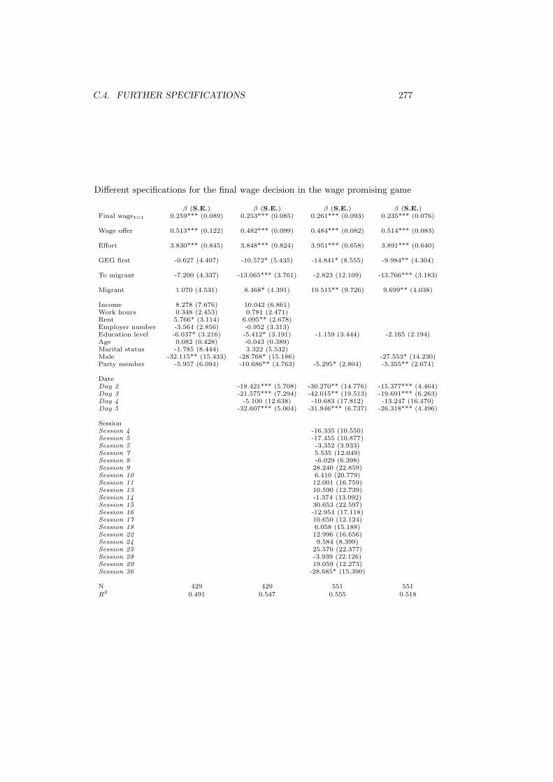
C.4. FURTHER SPECIFICATIONS 277
Different specifications for the final wage decision in the wage promising game
β (S.E.) β (S.E.) β (S.E.) β (S.E.)Final waget=1 0.259*** (0.089) 0.253*** (0.085) 0.261*** (0.093) 0.235*** (0.076)
Wage offer 0.513*** (0.122) 0.482*** (0.099) 0.484*** (0.082) 0.514*** (0.083)
Effort 3.830*** (0.845) 3.848*** (0.824) 3.951*** (0.658) 3.891*** (0.640)
GEG first -0.627 (4.407) -10.572* (5.435) -14.841* (8.555) -9.984** (4.304)
To migrant -7.200 (4.337) -13.065*** (3.761) -2.823 (12.109) -13.766*** (3.183)
Migrant 1.070 (4.531) 8.468* (4.391) 19.515** (9.726) 9.699** (4.038)
Income 8.278 (7.676) 10.042 (6.861)Work hours 0.348 (2.453) 0.781 (2.471)Rent 5.766* (3.114) 6.095** (2.678)Employer number -3.564 (2.856) -0.952 (3.313)Education level -6.037* (3.216) -5.412* (3.191) -1.159 (3.444) -2.165 (2.194)Age 0.082 (0.428) -0.043 (0.389)Marital status -1.785 (8.444) 3.322 (5.532)Male -32.115** (15.433) -28.768* (15.186) -27.553* (14.230)Party member -5.957 (6.094) -10.686** (4.763) -5.295* (2.804) -5.355** (2.674)
DateDay 2 -18.421*** (5.708) -30.270** (14.776) -15.377*** (4.464)Day 3 -21.575*** (7.294) -42.015** (19.513) -19.691*** (6.263)Day 4 -5.100 (12.638) -10.683 (17.812) -13.247 (16.470)Day 5 -32.607*** (5.004) -31.946*** (6.737) -26.318*** (4.496)
SessionSession 4 -16.335 (10.550)Session 5 -17.455 (10.877)Session 5 -3.352 (3.933)Session 7 5.535 (12.049)Session 8 -6.029 (6.398)Session 9 28.240 (22.859)Session 10 6.410 (20.779)Session 11 12.001 (16.759)Session 13 10.590 (12.739)Session 14 -1.374 (13.092)Session 15 30.653 (22.597)Session 16 -12.954 (17.118)Session 17 10.650 (12.124)Session 18 6.058 (15.188)Session 22 12.996 (16.656)Session 24 9.584 (8.399)Session 25 25.570 (22.377)Session 28 -3.939 (22.126)Session 29 19.059 (12.273)Session 36 -28.685* (15.390)
N 429 429 551 551R2 0.491 0.547 0.555 0.518

278 APPENDIX C. APPENDIX TO CHAPTER 8
Different specifications for the effort decision in the gift exchange game
β (S.E.) β (S.E.) β (S.E.) β (S.E.)Effortt=1 0.240*** (0.053) 0.242*** (0.053) 0.280*** (0.049) 0.255*** (0.044)
Wage offer 0.049*** (0.008) 0.047*** (0.008) 0.057*** (0.007) 0.051*** (0.007)
Effortt−1 0.387*** (0.061) 0.372*** (0.059) 0.295*** (0.052) 0.337*** (0.050)
GEG first 0.173 (0.308) -0.145 (0.380) 1.332*** (0.345) -0.142 (0.346)
To migrant -0.769** (0.358) -0.760** (0.372) -1.416* (0.825) -0.833** (0.325)
Migrant 0.080 (0.365) -0.244 (0.380) -1.802* (0.923) 0.227 (0.286)
Income -0.282 (0.243) -0.430 (0.289)Work hours 0.316* (0.175) 0.337* (0.174)Rent 0.175 (0.176) 0.175 (0.183)Employer number 0.194 (0.280) 0.194 (0.282)Education level -0.058 (0.291) -0.193 (0.323)Age 0.061* (0.031) 0.057* (0.032) 0.068*** (0.021) 0.065*** (0.021)Marital status 1.135 (0.689) 1.027 (0.675)Party member -0.703 (0.521) -0.909* (0.733) -0.672 (0.488) -0.530 (0.454)
DateDay 2 -0.721 (0.582) 2.498** (1.061) -0.118 (0.443)Day 3 -0.639 (0.713) 2.828* (1.510) -0.544 (0.615)Day 4 -1.810** (0.871) -0.789 (1.427) -1.269* (0.746)Day 5 -0.866 (0.681) -0.388 (0.868) -0.213 (0.595)
SessionSession 4 1.359 (1.937)Session 5 1.334 (1.379)Session 6 1.369* (0.769)Session 7 -1.007 (1.330)Session 8 1.900* (1.139)Session 9 -4.648*** (1.289)Session 10 -0.410 (1.215)Session 11 -2.046 (1.256)Session 12 1.372 (1.351)Session 13 -1.304 (0.927)Session 14 -1.139 (1.158)Session 15 -4.100*** (1.429)Session 16 -1.636 (1.318)Session 17 1.319 (1.026)Session 18 0.170 (1.252)Session 22 -0.662 (1.296)Session 24 -0.792 (1.493)Session 25 -3.300 (2.141)Session 28 3.000*** (1.045)Session 29 1.481 (1.461)Session 36 1.708*** (0.390)
N 602 602 812 812R2 0.545 0.548 0.558 0.522
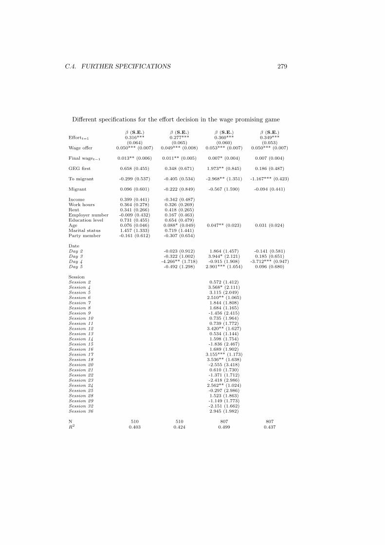
C.4. FURTHER SPECIFICATIONS 279
Different specifications for the effort decision in the wage promising game
β (S.E.) β (S.E.) β (S.E.) β (S.E.)Effortt=1 0.316*** 0.277*** 0.360*** 0.349***
(0.064) (0.065) (0.060) (0.053)Wage offer 0.050*** (0.007) 0.049*** (0.008) 0.053*** (0.007) 0.050*** (0.007)
Final waget−1 0.013** (0.006) 0.011** (0.005) 0.007* (0.004) 0.007 (0.004)
GEG first 0.658 (0.455) 0.348 (0.671) 1.973** (0.845) 0.186 (0.487)
To migrant -0.299 (0.537) -0.405 (0.534) -2.968** (1.351) -1.167*** (0.423)
Migrant 0.096 (0.601) -0.222 (0.849) -0.567 (1.590) -0.094 (0.441)
Income 0.399 (0.441) -0.342 (0.487)Work hours 0.364 (0.278) 0.326 (0.269)Rent 0.341 (0.266) 0.418 (0.265)Employer number -0.009 (0.432) 0.167 (0.463)Education level 0.731 (0.455) 0.654 (0.479)Age 0.076 (0.046) 0.088* (0.049) 0.047** (0.023) 0.031 (0.024)Marital status 1.457 (1.333) 0.719 (1.441)Party member -0.161 (0.612) -0.307 (0.654)
DateDay 2 -0.023 (0.912) 1.864 (1.457) -0.141 (0.581)Day 3 -0.322 (1.002) 3.944* (2.121) 0.185 (0.651)Day 4 -4.266** (1.718) -0.915 (1.908) -3.712*** (0.947)Day 5 -0.492 (1.298) 2.901*** (1.054) 0.096 (0.680)
SessionSession 2 0.572 (1.412)Session 4 3.568* (2.111)Session 5 3.115 (2.049)Session 6 2.510** (1.065)Session 7 1.844 (1.808)Session 8 1.684 (1.165)Session 9 -1.456 (2.415)Session 10 0.735 (1.964)Session 11 0.739 (1.772)Session 12 3.420** (1.627)Session 13 0.534 (1.144)Session 14 1.598 (1.754)Session 15 -1.836 (2.467)Session 16 1.689 (1.902)Session 17 3.155*** (1.173)Session 18 3.536** (1.638)Session 20 -2.555 (3.418)Session 21 0.610 (1.730)Session 22 -1.371 (1.712)Session 23 -2.418 (2.986)Session 24 2.562** (1.024)Session 25 -0.297 (2.986)Session 28 1.523 (1.863)Session 29 -1.149 (1.773)Session 32 -2.151 (1.662)Session 36 2.945 (1.982)
N 510 510 807 807R2 0.403 0.424 0.499 0.437
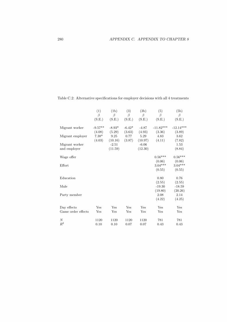
280 APPENDIX C. APPENDIX TO CHAPTER 8
Table C.2: Alternative specifications for employer decisions with all 4 treatments
(1) (1b) (3) (3b) (5) (5b)β β β β β β
(S.E.) (S.E.) (S.E.) (S.E.) (S.E.) (S.E.)
Migrant worker -9.57** -8.93* -6.42* -4.87 -11.82*** -12.14***(4.08) (5.29) (3.63) (4.93) (3.36) (3.89)
Migrant employer 7.38* 9.25 0.77 5.29 4.83 3.62(4.03) (10.16) (3.87) (10.97) (4.11) (7.82)
Migrant worker -2.51 -6.06 1.53and employer (11.59) (12.30) (8.84)
Wage offer 0.56*** 0.56***(0.06) (0.06)
Effort 3.04*** 3.04***(0.55) (0.55)
Education 0.80 0.76(2.55) (2.55)
Male -19.30 -18.59(19.80) (20.26)
Party member 2.08 2.14(4.22) (4.25)
Day effects Yes Yes Yes Yes Yes YesGame order effects Yes Yes Yes Yes Yes Yes
N 1120 1120 1120 1120 781 781R2 0.10 0.10 0.07 0.07 0.43 0.43

C.4. FURTHER SPECIFICATIONS 281
Table C.3: Alternative specifications for employer decisions with all 4 treatmentsand further controls
(2) (2b) (4) (4b) (6) (6b)β β β β β β
(S.E.) (S.E.) (S.E.) (S.E.) (S.E.) (S.E.)
Migrant worker -3.65** -3.00 -2.42 -1.72 -13.77*** -13.76***(1.58) (1.96) (1.77) (2.15) (3.18) (3.61)
Migrant employer 1.25 3.17 -2.30 -0.26 9.70** 9.75(1.45) (3.15) (1.67) (3.52) (4.04) (7.09)
Migrant worker -2.58 -2.74 -0.06and employer (3.62) (4.02) (8.67)
Wage offer in t=1 0.19*** 0.19*** 0.10** 0.10**(0.04) (0.04) (0.04) (0.04)
Wage offerlag 0.59*** 0.59*** 0.61*** 0.61***(0.05) (0.05) (0.06) (0.06)
Effortlag 0.15 0.15 0.20 0.21(0.19) (0.19) (0.22) (0.22)
Effort 3.89*** 3.89***(0.64) (0.64)
Wage offer 0.51*** 0.51***(0.08) (0.08)
Final Wage in t=1 0.23*** 0.23***(0.08) (0.08)
Education -2.16 -2.16(2.19) (2.21)
Male -27.55* -27.59*(14.23) (14.64)
Party member -5.35** -5.35*(2.67) (2.72)
Day effects Yes Yes Yes Yes Yes YesGame order effects Yes Yes Yes Yes Yes YesN 980 980 980 980 551 551R2 0.57 0.57 0.51 0.51 0.52 0.52

282 APPENDIX C. APPENDIX TO CHAPTER 8
Table C.4: Alternative specifications for worker decisions with all 4 treatments
(7) (7b) (9) (9b)β β β β
(S.E.) (S.E.) (S.E.) (S.E.)
Migrant employer -1.15** -1.63 -1.29*** -1.58(0.57) (1.07) (0.47) (0.97)
Migrant worker -0.42 -0.60 -0.65 -0.75(0.61) (0.71) (0.51) (0.59)
Migrant worker 0.66 0.39and employer (1.24) (1.17)
Wage offer 0.06*** 0.06*** 0.06*** 0.06***(0.01) (0.01) (0.01) (0.01)
Age 0.10*** 0.10*** 0.05* 0.05*(0.03) (0.03) (0.03) (0.03)
Party member -1.98*** -1.95***(0.70) (0.73)
Day effects Yes Yes Yes YesGame order effects Yes Yes Yes Yes
N 928 928 1088 1088R2 0.28 0.28 0.30 0.30

C.4. FURTHER SPECIFICATIONS 283
Table C.5: Alternative specifications for worker decisions with all 4 treatmentsand further controls
(8) (8b) (10) (10b)β β β β
(S.E.) (S.E.) (S.E.) (S.E.)
Migrant employer -0.83** -0.98* -1.17*** -1.33(0.33) (0.58) (0.42) (1.01)
Migrant worker 0.23 0.17 -0.09 -0.14(0.29) (0.38) (0.44) (0.46)
Migrant worker 0.21 0.22and employer (0.70) (1.12)
Wage offer 0.05*** 0.05*** 0.05*** 0.05***(0.01) (0.01) (0.01) (0.01)
Effort in t=1 0.26*** 0.25*** 0.35*** 0.35***(0.04) (0.04) (0.05) (0.05)
Effortlag 0.34*** 0.34***(0.05) (0.05)
Final Wagelag 0.01 0.01(0.00) (0.00)
Age 0.07*** 0.07*** 0.03 0.03(0.02) (0.02) (0.02) (0.02)
Party member -0.53 -0.52(0.45) (0.44)
Day effects Yes Yes Yes YesGame order effects Yes Yes Yes Yes
N 812 812 807 807R2 0.52 0.52 0.44 0.44

284 APPENDIX C. APPENDIX TO CHAPTER 8

Part VI
Appendix to Part III
285


Appendix D
Appendix to chapter 10
287

288 APPENDIX D. APPENDIX TO CHAPTER 10
D.1 Experimental instructions
The following sections document the instructions of the different stages of the
game (section titles were not provided to participants)
D.1.1 Public good game (PGG)
General introduction
Instructions
You are about to begin the economic experiment. Before the experimental ses-
sion starts, please read the following instructions carefully. This is important
because the final payment you receive for participating in the experiment can be
affected by how well you understand the instructions and your decisions during
the game.
Please note that all information provided during the experiment is treated con-
fidentially.
You are prohibited from communicating with other participants during the ex-
periment.
All the decisions you make during the game are anonymous in the sense that
other participants cannot attribute decisions to other individuals.
If you have any questions now, or during this experiment, please indicate this
by raising your hand. Do not talk to other participants
The experiment consists of several games and task solving exercises. A game in
this context means that players make decisions that directly or indirectly affect
the outcomes of other players. Those games are played for a (small) number of
consecutive rounds, during which the same game will be repeated. At the be-
ginning of each game, you will be informed about the number of rounds played.
The task solving exercises will always be played for only one round.
The dollar values you see on the computer screens are ’experimental dollars’.
Your income and payoffs are calculated using these experimental dollars. Your
decisions and answers hence determine how much you will receive for partic-
ipating in the experiment. The conversion rate from experimental dollars to
Australian dollars is:
D.1. EXPERIMENTAL INSTRUCTIONS 289
100 experimental dollars = 5 Australian dollars.
PGG without punishment
Instructions
In the following game you are supplied with 10 experimental dollars at the
beginning of each round. You can use this amount to either keep it to yourself
or to contribute up to 10 experimental dollars to a common pool.
The common pool is made up of the contributions from 3 players and jointly
owned by them. All players will remain in their group for all rounds of this
game. A group consists of three people.
After all group members have made their contributions to the pool, the total
contributions will be multiplied by the factor 2. Subsequently the pool will be
equally split between the group members. I.e. the split is such that each member
of the pool receives an equal amount. This also means that the redistribution
will be independent of what a player previously contributed to the common
pool.
All decisions made in the following rounds, both yours and those of others will be
anonymous; that is, you will be unable to observe which player has contributed
which amount to the common pool.
The game will be played for 4 rounds.
Finally, please note that contributions need to be multiples of one experimental
dollar.
PGG with punishment
Instructions modification
For the next 4 rounds the game will continue to be played as before. I.e. you
can make contributions to a common pool, which are then multiplied by the
factor 2 and equally split between the members of the group.
However, contrary to before, it will be possible to determine which player has
contributed what amount. Hence, in an additional step, all members of a group
will be informed about the other players’ contributions.
Having received this information, group members can then decide if they want to
punish other players for their contributions. If a player is punished, it will mean
that he has to pay a ”fine” of 4 experimental dollars, which will be subtracted

290 APPENDIX D. APPENDIX TO CHAPTER 10
from his final payoff.
The decision to punish other players will, however, be costly for the player who
punishes others. For every punishment made, the punishing player will incur a
cost of 2 experimental dollars.
It will not be possible to determine which player has punished other players.
That is, the punishment is anonymous.
D.1.2 Arithmetic questions pt.1
Instructions
In the following section you will be asked to solve two different types of math-
ematical questions. The questions will ask you to either solve the sum of the
digits provided, or the product of the digits provided.
To solve the questions you have to make the following calculations to find the
solution:
For the sum of digits, add up all the digits. For example, to solve 25901, arrive
at the solution by calculating 2+5+9+0+1 = 17.
For the product of digits, multiply the digits. For example, to solve 3172, arrive
at the solution by calculating 3*1*7*2 = 42.
The difficulty of the questions will increase with when proceeding in the game.
Please also note that questions for which you will have to calculate the sum of
digits and questions for which you have to calculate the product of digits will
randomly change between periods. Hence, make sure you check the task at the
beginning of each question.
Each correct answer is worth 8 experimental dollars. There is a time-limit of 10
minutes for all questions (on average 30 seconds per question).
D.1.3 Dictator game (DG)
DG without punishment
Instructions
For the following rounds, a new game will be played. Please go through the
instructions carefully again.
In this game, players are assigned the role of the transferring player or the role
of the recipient.

D.1. EXPERIMENTAL INSTRUCTIONS 291
The transferring player is supplied with 10 experimental dollars. The transfer-
ring player can then either keep this amount or transfer up to 10 experimental
dollars a second player who has been randomly matched in the role of the recip-
ient. The recipient will receive the transfer, but will not have the opportunity
to communicate anything back to the transferring player.
The game will be repeated for 2 rounds.
Please note that all transfers need to be multiples of one experimental dollar.
DG with punishment
Instructions modification
In the next rounds, the game will again be slightly altered. Again, there will be
a transferring player and a recipient. But additionally, after the decisions of the
transferring players have been made, the amount of their transfers will be made
available to a third player, who is unaffected by the transfer decision. That is,
this player is neither a transferrer nor a recipient in the transaction.
The third player can then evaluate if the transfer has been appropriate. If the
evaluating player thinks that the transfer has not been appropriate, the third
player can impose a fine on the transferring player of 4 experimental dollars.
However, for imposing the fine, the third (punishing) player will have to pay 2
experimental dollars.
Again, the game will be repeated for 2 rounds.
D.1.4 Betting game
Instructions
In the following section, all players will solve test questions that are similar to
those solved earlier in the experiment. As before, for every question correctly
answered, they will receive 8 experimental dollars.
Additionally to solving questions yourself, you have randomly been assigned an-
other player on whose performance you can bet. Similarly, another player will
be able to bet on your performance. The table below provides you with infor-
mation on the betting odds. There is only one fixed amount of 30 experimental
dollars, which you can place as a bet.
The number of correct answers on which you place your bet is a minimum num-
ber; that is, when your assigned player answers more questions correctly than

292 APPENDIX D. APPENDIX TO CHAPTER 10
you have chosen, you will still win your bet. If the number of correctly answered
questions is below your bet, you will lose. The odds on your bet increase with
the number of questions that you bet your assigned player will answer correctly.
Example: If you bet that the player that has been assigned to you will answer 10
questions correctly, you will receive 2*30 experimental dollars if your assigned
player answers 10 or more questions correctly and will lose your bet of 30 if your
assigned player answers less than 10 questions correctly.
Please also note for your further information:
The average number of questions correctly answered in the first round was .
Please tick the number of questions that you think will be answered correctly
on the lower right to make your bet.
Table D.1: Table of betting odds for participants
Number of Factor multipliedcorrect answers with 30 in
case of winning4 1.28 1.510 212 2.514 316 418 620 10
D.1.5 Arithmetic questions pt.2
Instructions
In the following section you will again be asked to solve two different types of
mathematical questions, i.e. to either solve the sum of the digits provided, or
the product of the digits provided. To solve the questions you have to make the
following calculations to find the solution:
For the sum of digits, add up all the digits. For example, to solve 25901, arrive
at the solution by calculating 2+5+9+0+1 = 17.
For the product of digits, multiply the digits. For example, to solve 3172, arrive
at the solution by calculating 3*1*7*2 = 42.
The difficulty of the questions will increase with when proceeding in the game.
Please also note that questions for which you will have to calculate the sum of

D.1. EXPERIMENTAL INSTRUCTIONS 293
digits and questions for which you have to calculate the product of digits will
randomly change between periods. Hence, make sure you check the task at the
beginning of each question.
Each correct answer is worth 8 experimental dollars. As pointed out before,
furthermore a randomly chosen second player has been able to place a bet on
your performance and will win or lose depending on your performance.
Again, there is a time-limit of 10 minutes for all questions (on average 30 seconds
per question).
D.1.6 Bidding game
Instructions
For the next 4 rounds the following game will be played: At the beginning of
each round, all participants will be provided with 10 experimental dollars that
they use for bidding for a common pot. Bids can be made between 0 and 10
experimental dollars. All bids will directly be paid into the pot.
Remaining money out of 10 that has not been used for bidding in a period will
be paid to the player at the end of the round.
The size of the pot will be made up of all bids that have been submitted by all
players plus an additional amount of 10 experimental dollars, which has been
placed in the pot by the experimenter. After all players have placed their bids,
the pot will be distributed between the players as follows:
• The player with the highest bid will be paid one half of the money in the
pot.
• The player with the second highest bid will be paid one third of the money
in the pot.
• The player with the lowest bid will be paid one sixth (the rest) of the
money in the pot.
• In case two or three players submit an equal bid, they will equally share the
amount that they would have won together. For example, if the highest
bid is shared by two players, then each of them will receive one half of
(one half + one third), i.e. 5/12.
294 APPENDIX D. APPENDIX TO CHAPTER 10
D.1.7 Ability test
Now you will be asked various types of questions that must be completed with-
out a calculator or any other aid.
Directions (Please Read Carefully)
This test contains 50 questions that increase in difficulty. It is unlikely that you
will finish all of them, but do your best.
After you start you will have 12 minutes to provide as many correct answers as
you can. Work carefully but do not spend too much time on any one question.
You can skip questions but you cannot return to unanswered questions on pre-
vious screens. Be sure to write your answers in the fields provided. Before you
begin taking this test, please answer the Sample Questions below.

interpersonal communication
computer work
problem solving/mental activity
driving a car
public transport
walking/ cycling
sports
housework
eating/ drinking
TV
personal hygiene
relaxation/resting
sleeping
other activities
mood
work/personal
alone / in a pair in a group
additional comments
J P J P J P J P J P J P J P J P J P J P J P
TIME
= go
od m
ood
= ba
d m
ood
J
= w
ork
P
= pr
ivat
e
= al
one
=
in a
pai
r =
in a
gro
up &
= p
hone
|
pl
ease
sig
n ac
tiviti
es a
t the
sam
e tim
e w
ith a
n .
Fir
st n
am
e:
L
ast
na
me:
Be
gin
nin
g o
f M
easu
rem
en
t:
Ple
ase
inse
rt t
ime
in t
he
corr
esp
on
din
g c
olu
mn
and
an
d m
ark
you
r m
oo
d a
t th
e ti
me.

= go
od m
ood
= ba
d m
ood
J
= w
ork
P
= pr
ivat
e
= al
one
=
in a
pai
r =
in a
gro
up &
= p
hone
|
pl
ease
sig
n ac
tiviti
es a
t the
sam
e tim
e w
ith a
n .
interpersonal communication
computer work
problem solving/mental activity
driving a car
public transport
walking/ cycling
sports
housework
eating/ drinking
TV
personal hygiene
relaxation/resting
sleeping
other activities
mood
work/personal
alone / in a pair in a group
additional comments
J P J P J P J P J P J P J P J P J P J P J P J P J P J P
TIME

Appendix E
Technical Appendix onHRV
297
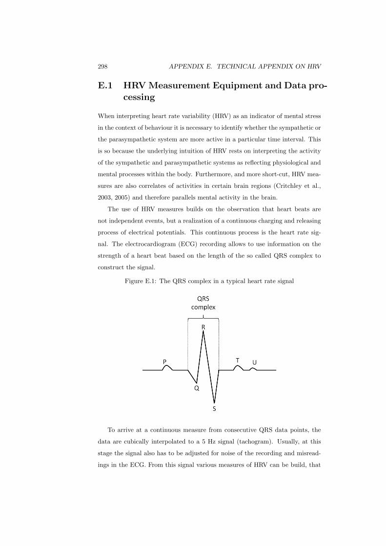
298 APPENDIX E. TECHNICAL APPENDIX ON HRV
E.1 HRV Measurement Equipment and Data pro-cessing
When interpreting heart rate variability (HRV) as an indicator of mental stress
in the context of behaviour it is necessary to identify whether the sympathetic or
the parasympathetic system are more active in a particular time interval. This
is so because the underlying intuition of HRV rests on interpreting the activity
of the sympathetic and parasympathetic systems as reflecting physiological and
mental processes within the body. Furthermore, and more short-cut, HRV mea-
sures are also correlates of activities in certain brain regions (Critchley et al.,
2003, 2005) and therefore parallels mental activity in the brain.
The use of HRV measures builds on the observation that heart beats are
not independent events, but a realization of a continuous charging and releasing
process of electrical potentials. This continuous process is the heart rate sig-
nal. The electrocardiogram (ECG) recording allows to use information on the
strength of a heart beat based on the length of the so called QRS complex to
construct the signal.
Figure E.1: The QRS complex in a typical heart rate signal
To arrive at a continuous measure from consecutive QRS data points, the
data are cubically interpolated to a 5 Hz signal (tachogram). Usually, at this
stage the signal also has to be adjusted for noise of the recording and misread-
ings in the ECG. From this signal various measures of HRV can be build, that

E.1. HRV MEASUREMENT EQUIPMENT AND DATA PROCESSING 299
describe how the heart rate changes over different time intervals. These inter-
vals can be long (i.e. to explore daytime variation) or very short covering only
minutes or even seconds.
Here HRV is represented as a power spectral density (PSD). This HRV es-
timation process builds on the fact that the heart rate signal can be explained
using a decomposition into time-frequency distributions.1 The PSD assigns a
power value to each frequency or wave length for each point in time (more ex-
actly for each time interval). The heart rate signal is thus represented in terms
of importance (power) of a particular wave (frequency) at a point in time.
The estimation of these PSD is, however, potentially dependent on the es-
timation technique employed. The three most commonly used time-frequency
decomposition methods are described in more detail below. These methods are
(i) the Short-term Fast Fourier Transformation (SFFT), (ii) the Autoregressive
Spectral Estimation (AR) and (iii) the Smoothed Pseudo Wigner-Ville Distri-
bution (SPWVD, a wavelet transformation). The three methods have different
properties with respect to accuracy and smoothness, which will be discussed
and evaluated following a brief description of these estimation techniques.
First, as mentioned in the context of linking cardiological and behavioural
data the effects of sympathetic and parasympathetic stimulation on the heart
rate is of primary interest. Activity of the sympathetic system has been linked
to so called low frequency (LF) [0.033 - 0.15 Hz] changes in the heart rate
signal, parasympathetic activity to high frequency (HF) [0.15 - 0.4 Hz] changes.
Daytime variation and long- to mid-term changes in the heart rate signal are
of minor interest. It is therefore necessary to eliminate any slowly varying
processes (waves that have a length of more than 27 seconds [ 0.033 Hz]) to
get accurate estimates. This process, called detrending, was conducted using a
standard DWT wavelet filter (Wiklund et al., 1997).
E.1.1 Estimation of the power spectral density (PSD)
For all of the following estimation methods a number of parameters have to
be considered. First, as mentioned before, there is a trade-off between time
resolution and frequency resolution. Consequently, one has to decide on the
1For example a composition of shorter and longer sine and cosine waves; for a more intuitiveunderstanding time-frequency distributions are in the following also referred to as “waves”.
300 APPENDIX E. TECHNICAL APPENDIX ON HRV
resolution of both. The lowest feasible time resolution is 27 seconds, which
corresponds to the lower end of the LF. For this time resolution a reasonable
frequency resolution would be 0.001 Hz, which results in a total of 512 frequency
bins. Finally, a second time resolution has to be chosen, which determines the
distance between two time points for which a new estimation is done. Since
estimations are over all values within a certain window, for all methods applied
the time window is adjusted with a Gaussian or Hamming scaling window, to
give more emphasis to the signal at the centre of the time window. In the case of
the wavelet transform the same procedure is also used to amplify the frequency
windows.
Short-term Fast Fourier Transformation (SFFT)
The oldest and simplest estimation method is the Fourier Transformation (FT).
The most commonly used algorithm for computation purposes is the Fast Fourier
Transformation (FFT). It is based on the principle, that any finite signal s can
be transformed into a series of parametrized sine and cosine functions. This
allows for estimates of the strength k of the frequency ω.
s(t) = α0 +
∞∑k=1
(αk cos(kωt) + βk sin(kωt)) (E.1)
The parameters αk and βk allow to deduct the desired PSD. The FFT is
a very well suited method for overlapping periodic signals. Unfortunately the
heart rate variation is to a large extend not periodic and time varying. The
common solution to this issue is to take short time intervals (that correspond
to the period of the longest frequency that is likely to be observed), detrend
this signal and apply the FFT after the detrending (short-term FFT, SFFT).
However, as this method is not very well suited to detect the isolated, short,
non-periodic changes in the heart rate, the SFFT is mainly used as a reference
point for other methods.
Autoregressive Spectral Estimation (AR)
Another widely used methodology to obtain the PSD of a signal is to fit an
autoregressive model of the form:

E.1. HRV MEASUREMENT EQUIPMENT AND DATA PROCESSING 301
Xt + α1Xt−1 + ...+ αMXt−M = εt (E.2)
where εt is a white noise process with a constant variance σ2. The PSD
estimate h(.) for different frequencies ω can be determined as:
h(ω) =σ2ε
2π
1
|1 +∑Mk=1 αke
−iωk|2(E.3)
where α1, ..., αM are the estimated model coefficients (Akaike, 1969). Esti-
mation with any order M bigger than 50 has been shown to yield a good “finite
order” approximation of the heart rate signal. The specific estimation technique
used goes back to a “maximum entropy” method first proposed by Burg (1968).
Spyers-Ashby et al. (1998) provide an overview for using both the SFFT and
the AR estimation techniques with physiological data.
Wavelet analysis using the Smoothed Pseudo Winger-Ville Distribu-tion (SPWVD)
The most recent estimation method is a wavelet analysis (Kaiser, 1994). The
intuition behind wavelet methods is that the signal is not simply cut into one
specific time window, but into a whole series of different windows. Each of these
windows is matched to a set of short periodic functions with certain frequen-
cies ω to obtain a power estimate. The resulting time-scale representation is
a collection of time-frequency distributions with different time and frequency
resolutions.
A suitable technique for HRV estimation is building the Smoother Pseudo
Wigner-Ville Distribution (SPWVD) (Seong et al., 2004). This method con-
denses the time-scale representation of the wavelet transform into a single time-
frequency distribution with a high time-frequency resolution.
PSDWV (t, ω) =
∫Wω(τ)×
[∫Wt(u− t)x(u+
τ
2)x∗(u+
τ
2)du
]e−iωtdτ
(E.4)
302 APPENDIX E. TECHNICAL APPENDIX ON HRV
Comparison and Evaluation of the estimation approaches in the con-text of HRV measurement
While the SFFT and the AR methods are well-established in the literature and
provide with reliable results, both techniques suffer from the trade-off between
time and frequency resolution. The reason for this is that both methods have
to use a predefined time window. This problem goes back to the Heisenberg
uncertainty principle; it is strictly not possible to get the exact frequency and
the exact time of occurrence of this frequency in the heart rate signal. In
comparison, the SPWVD technique allows for a much finer grade. The problem
that the result will contain overlapping time intervals, based on the same data
can be mitigated by using averages of the data. However, the SPWVD is not
yet used that frequently in practice. Therefore, it seems advisable to check the
results for consistency with the other two methods and to ensure that no major
discrepancies have arisen.
E.1.2 Data Collection and QRS detection
The heart rate measurement equipment used was the non-intrusive Holter Medilog
ECG Recorder AR12. This monitoring device has a pocket-size (10x7x2.5cm)
and is attached to the chest of the human subject using three conducting elec-
trodes. The monitoring device records the ECG with a high sampling rate of
4096 Hz. Furthermore, it records respiration levels and has a build-in QRS
detection algorithm. The data recorded is stored on an CF disk and can be
read using Medilog’s Darwin software; alternatively, the data can be exported
into a number of data formats (such as Matlab as was done here). In these
formats the raw recording data can be used for more user-specific analysis (such
as the application of the frequency distribution estimation methods described
above). To reduce the potential of irregularities and noisy readings, the heart
rate monitor function was tested using the IrDA (Infrared Data Association)
interface before the beginning of each recording session.