The Implicit Cost of Carbon AbatementDuring the COVID-19 Pandemic

EEA 2021. August 26th, 2021.

Natalia Fabra,∗ Aitor Lacuesta,‡ and Mateus Souza∗

∗ Universidad Carlos III de Madrid, EnergyEcoLab‡ Bank of Spain

1 / 17

Motivation

2 / 17

Motivation

Impact of the pandemic on carbon emissions:

Is there a silver lining? If so, how thick is it?

EU Green Deal:

By 2050, reach net zero CO2 emissions by 2050

By 2030, reduce emissions by at least 55% vs 1990 levels

Debate on how to achieve those goals:

Is it possible without sacrificing economic growth?

Or can we decouple growth from emissions?

What are the implicit costs of different strategies?

We focus on the case of Spain and its power sector.

3 / 17

Research Question

What are the implicit costs of carbon abatement accordingto alternative strategies?

1 Slowing down economic activity:

Pandemic as a natural experimentCaveat: Pandemic was a shock, not planned “degrowth”Pandemic is proxy of slow down, holding economic structurefixed

2 Investing in renewables:How much investment in renewables would we need to achievethe same carbon abatement as that observed during thepandemic?Can be considered as part of a decoupling strategy

4 / 17

Research Question

What are the implicit costs of carbon abatement accordingto alternative strategies?

1 Slowing down economic activity:

Pandemic as a natural experimentCaveat: Pandemic was a shock, not planned “degrowth”Pandemic is proxy of slow down, holding economic structurefixed

2 Investing in renewables:How much investment in renewables would we need to achievethe same carbon abatement as that observed during thepandemic?Can be considered as part of a decoupling strategy

4 / 17

Research Question

What are the implicit costs of carbon abatement accordingto alternative strategies?

1 Slowing down economic activity:

Pandemic as a natural experimentCaveat: Pandemic was a shock, not planned “degrowth”Pandemic is proxy of slow down, holding economic structurefixed

2 Investing in renewables:How much investment in renewables would we need to achievethe same carbon abatement as that observed during thepandemic?Can be considered as part of a decoupling strategy

4 / 17

Steps of the analysis

1 We measure the effects of the pandemic on emissionsreductions.

Counterfactual predictions in the power sector.Emissions from other sectors (from external references).

2 We measure the pandemic effects on the Spanish economy.

Counterfactual forecasts of GDP.

−→ After steps 1 and 2, calculate implicit cost of carbonfrom slowing down economic activity

3 Simulate investments in renewables necessary to achieveCO2 reductions similar to those observed in the power sectorduring the pandemic.

4 Compare the implicit cost of carbon abatement from thepandemic versus from investing in renewables.

5 / 17

Predicting Counterfactual Electricity Consumption

Objective:Predict counterfactual electricity consumption in absence ofthe pandemic

Obtain precise hourly predictions, which will be used later inelectricity market simulationsUse only covariates that are not affected by the pandemic

Data:Hourly consumption in Spain from 2015-2020Weather variables: temperature, precipitation, wind speed, andwind directionHolidaysDate/time fixed effects (seasonality)Time trends

6 / 17

Predicting Counterfactual Electricity Consumption

Predictive machine learning model of consumption:

Yt(0) = g(Xt) + εt

Covariates Xt : weather and date/time fixed effects

Model trained and cross-validated with past data (2015-2019)

Model selected based on out-of-sample performanceUsing forward chaining cross-validation (Hyndman andAthanasopoulos, 2018):

g(): Gradient Boosted Trees (GBT; Chen and Guestrin, 2016)

Impact of the pandemic on electricity demand:

bt = Yt(1)− Yt(0) = Yt(1)− g(Xt)

Main assumption: relationship g() between energy consumptionand covariates would not have changed from 2019-2020.

7 / 17

Forward Chaining Cross-Validation

Choose model based on prediction errors (RMSE) in 2019

GBT results in RMSE of 809 MWh; compared to avg. hourlyconsumption in 2019 = 28,528 MWh; or std. dev. = 4,525.

8 / 17

Cross-Validation Results – ML

Average out-of-sample residual is less than 1% of average hourly consumption9 / 17

Cross-Validation Results – fixed effects model

Day of year FE; hour of day interacted with weather; lagged (up to 3) weather10 / 17

Counterfactual Consumption in the Power Sector

Notes: Based on 30-day moving averages.11 / 17

Counterfactual Emissions in the Power Sector

Use the hourly consumption estimates to simulate the hourlyelectricity market outcomes with and w/o the pandemic

Simulations based on De Frutos and Fabra (2012)

Identify which plants would have been dispatched −→ obtaincarbon intensity of the market

We take all else as given:

Hourly availability of renewablesMonthly hydro availabilityExisting capacity of gas/coal/nuclear plantsDaily prices of gas/coal/CO2Caveats: nuclear availability and gas/coal/CO2 prices mayhave changed

12 / 17

Counterfactual Emissions in the Power Sector

Use the hourly consumption estimates to simulate the hourlyelectricity market outcomes with and w/o the pandemic

Simulations based on De Frutos and Fabra (2012)

Identify which plants would have been dispatched −→ obtaincarbon intensity of the market

We take all else as given:

Hourly availability of renewablesMonthly hydro availabilityExisting capacity of gas/coal/nuclear plantsDaily prices of gas/coal/CO2Caveats: nuclear availability and gas/coal/CO2 prices mayhave changed

12 / 17

Simulated Change in Emissions from Power Sector

Spanish power sector carbon emissions, measured in MtCO2

Simulations With Simulations WithCounterfactual Demand Realized Demand Difference

Coal 3.23 3.08 0.15Gas 21.69 18.00 3.69Cogen + Others 11.16 10.87 0.29

Total 36.07 31.94 4.13

Notes: Assuming competitive market structure. Results from strategic equilibrium

presented in the paper.

Almost 90% of abatement due to reduced gas usage.

13 / 17

Emissions from Other Sectors

CO2 Emissions for Other Sectorsin Spain

MtCO2 Emissions

2019 2020 Diff. Pct. Diff.

Domestic Aviation 5.64 3.00 2.63 46.68Ground Transport 84.83 75.40 9.43 11.12Industry 62.25 55.63 6.62 10.64Residential 36.70 36.14 0.56 1.53

Source: (Carbon Monitor; Liu et al., 2020)

Total abatement in Spain during 2020 = 23.14 MtCO2

14 / 17

Counterfactual Economic Activity

Counterfactual GDP based on forecasts from Bank of Spain

Forecasts made at the end of 2019 (no info. about pandemic)

Total GDP loss in 2020: 169.37 Billion Euros

Implicit cost of carbon = 7,319 €/Ton CO215 / 17

Investing in Renewables

Power market simulations (De Frutos and Fabra, 2012)Vary types of investments: increase solar or wind capacityKeep simulations that yield the same emissions reductions inthe power sector as the pandemic

Investment Costs (M EUR)

Emission ReductionsTotal

Annualized Implicit Cost of Carbon(M Tons) Investment+O&M (EUR/Ton)

Pandemic 4.13 - - -Solar Investments 4.53 6,890.11 275.60 60.80Wind Investments 4.06 6,122.97 244.92 60.34

Notes: Assuming competitive market structure. Results from strategic equilibrium

presented in the paper. Costs from IRENA (2020).

The implicit cost of carbon under each strategy is:

1 Slowing down economic activity: 7,319 €/Ton CO22 Renewables: 60 €/Ton CO2

16 / 17

Investing in Renewables

Power market simulations (De Frutos and Fabra, 2012)Vary types of investments: increase solar or wind capacityKeep simulations that yield the same emissions reductions inthe power sector as the pandemic

Investment Costs (M EUR)

Emission ReductionsTotal

Annualized Implicit Cost of Carbon(M Tons) Investment+O&M (EUR/Ton)

Pandemic 4.13 - - -Solar Investments 4.53 6,890.11 275.60 60.80Wind Investments 4.06 6,122.97 244.92 60.34

Notes: Assuming competitive market structure. Results from strategic equilibrium

presented in the paper. Costs from IRENA (2020).

The implicit cost of carbon under each strategy is:

1 Slowing down economic activity: 7,319 €/Ton CO22 Renewables: 60 €/Ton CO2

16 / 17

Conclusions

Carbon abatement may be obtained by slowing down economicactivity and/or investing in renewables

1 Results suggest that simply halting growth is too costly

The magnitude of the losses versus the relatively smallabatement make that clearCarbon abatement was short-lived, while economic losses areexpected to be long-lasting

2 Investments in renewables can achieve abatement at muchlower cost

Renewables could even provide more benefits in terms ofeconomic stimulus

3 Of course, these strategies should be complemented with:

Improving energy efficiency, revolutionizing transport andmobility, etc.

17 / 17

Thank You!

Comments? Feedback? Questions?mateus.nogueira@uc3m.es

http://energyecolab.uc3m.es/

This Project has received funding from the European Research Council(ERC) under the European Union´s Horizon 2020 research and innovationprogramme (grant agreement No 772331).

References

Chen, Tianqi and Carlos Guestrin (2016). “XGBoost: A ScalableTree Boosting System”. arXiv:1603.02754.

De Frutos, Marıa-Angeles and Natalia Fabra (2012). “How toallocate forward contracts: The case of electricity markets”.European Economic Review 56(3), pp. 451–469.

Hyndman, Rob J and George Athanasopoulos (2018). Forecasting:principles and practice. OTexts. Chap. 5.10 - Time seriescross-validation.

IRENA (2020). Renewable Power Generation Costs in 2019.Tech. rep. International Renewable Energy Agency, Abu Dhabi.

Liu, Zhu, Philippe Ciais, Zhu Deng, Steven J Davis, Bo Zheng,Yilong Wang, Duo Cui, Biqing Zhu, Xinyu Dou, Piyu Ke, et al.(2020). “Carbon Monitor, a near-real-time daily dataset ofglobal CO 2 emission from fossil fuel and cement production”.Scientific data 7(1), pp. 1–12.

Appendix: Why Machine Learning?

ML flexibly accounts for nonlienarities and high-orderinteractions

Agnostic about which variables are most important

Agnostic about functional forms

Best out-of-sample performance

Will compare to fixed effects models

Appendix: Cross-Validation Results

Using RMSE as accuracy metric. Values are in MWh.

Panel A: Validation Year RMSE

Model ID 2016 2017 2018 2019

ML 1 1155.88 934.42 856.18 809.13ML 2 1160.67 984.78 871.45 815.45ML 3 1517.53 1219.22 1165.42 1063.05ML 4 1532.10 1266.84 1152.23 1083.03

FE 1 1786.17 1837.05 1878.91 1998.73FE 2 1856.67 1836.63 1890.78 2019.15FE 3 2931.66 1814.91 1899.57 2009.61FE 4 1936.32 1227.76 1361.87 1550.50

Compared to avg. hourly consumption in 2019 = 28,528 MWh; orstd. dev. = 4,525.

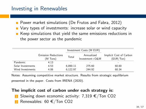
Appendix: Details on Specifications

Using RMSE as accuracy metric. Values are in MWh.

Panel B: Details on Model Specifications

Model ID ML Hyperparameters

ntrees max depth shrinkage minobspernode

ML 1 2000 10 0.05 20ML 2 2000 30 0.05 20ML 3 2000 10 0.5 20ML 4 2000 30 0.5 20

Model ID Fixed Effects Included

FE 1 Month of yearFE 2 Week of yearFE 3 Day of yearFE 4 Day of year; hour of day interacted with weather

Appendix: Inference With Machine Learning

Let bt be the effect of the pandemic.Yt(1) is realized demand, and Yt(0) is counterfactual demand

bt = Yt(1)− Yt(0)

bt = Yt(0) + bt − Yt(0)

−→ bt = bt + Yt(0)− Yt(0)

−→ bt = bt − rt

Where rt are residuals from the prediction of Yt(0)

Then we also have (assuming bt and rt independent):

Var(bt) = Var(bt) + Var(rt)

Note that rt cannot be observed, so we proxy it with the varianceof the (out-of-sample) residuals from 2019

Effect of the Pandemic on Electricity Consumption

Reduced electricity consumption by hour of the day

1st Partial Lockdown(March 11 - March 28)

Full Lockdown(March 29 - April 10)

Effect of the Pandemic on Electricity Consumption

Reduced electricity consumption by hour of the day

Partial Lockdowns(April 11 - August 14)

Rest of Year(August 15 - December 31)

Generation Mix in the Power Sector

(a) Realized consumption (b) Counterfactual consumption

Notes: Using data up to September 2020. Assuming competitive market structure.

Results from strategic equilibrium presented in the paper.

External Validity: France – Emissions

Sector MtCO2 Emissions

2019 2020 Diff. Pct. Diff.

Domestic Aviation 2.33 1.29 1.04 44.53Ground Transport 116.62 104.80 11.82 10.14Industry 61.67 54.47 7.20 11.67Residential 79.87 75.75 4.12 5.16

Counterfactual Realized Diff. Pct. Diff.

Power (lower bound) 22.68 21.79 0.90 3.95Power (upper bound) 171.28 164.50 6.77 3.95

Total (lower bound) 283.17 258.10 25.07 8.85Total (upper bound) 431.77 400.81 30.96 7.17

Lower bound assumes carbon intensity of 49 gCO2/kWh (avg. of sector)

Upper bound assumes carbon intensity of 370 gCO2/kWh (CCGTs)

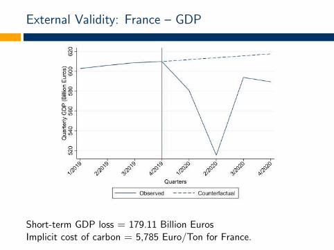
External Validity: France – GDP

Short-term GDP loss = 179.11 Billion EurosImplicit cost of carbon = 5,785 Euro/Ton for France.

External Validity: Italy – Emissions

Sector MtCO2 Emissions

2019 2020 Diff. Pct. Diff.

Domestic Aviation 1.89 1.00 0.89 47.02Ground Transport 91.13 81.63 9.50 10.42Industry 54.39 47.75 6.64 12.21Residential 74.95 73.92 1.04 1.38

Counterfactual Realized Diff. Pct. Diff.

Power (lower bound) 76.18 74.31 1.87 2.45Power (upper bound) 103.62 101.08 2.54 2.45

Total (lower bound) 298.54 278.61 19.93 6.68Total (upper bound) 325.98 305.38 20.60 6.32

Lower bound assumes carbon intensity of 272 gCO2/kWh (avg. of sector)

Upper bound assumes carbon intensity of 370 gCO2/kWh (CCGTs)

External Validity: Italy – GDP

Short-term GDP loss = 145.48 Billion EurosImplicit cost of carbon = 7,062 Euro/Ton for Italy.

Simulations Using Predictions from FE

Counterfactual Demand (FE Model) Realized Demand Difference

CO2 (M Ton) Competitive Strategic Competitive Strategic Competitive Strategic

Coal 3.36 3.87 3.08 3.52 0.28 0.35Gas 23.55 23.36 18.00 17.85 5.55 5.51Cogen + Others 11.21 11.56 10.87 11.49 0.34 0.07

Total 38.11 38.79 31.94 32.86 6.16 5.93

Abatement estimates are substantially higher with thesesimulations: assuming competitive behavior, abatement was 6.16Million Tons (almost 50% higher than those from ML).