THE IMPLICATIONS OF UNCERTAINTY FORMONETARY POLICY

Geoffrey Shuetrim and Christopher Thompson

Research Discussion Paper1999-10

November 1999

Economic Research Department

Reserve Bank of Australia

An earlier version of this paper was presented at the Reserve Bank ofNew Zealand workshop on Monetary Policy under Uncertainty, 29–30 June 1998.We thank participants at that conference for their comments, especiallyArthur Grimes, the paper’s discussant. The paper has also benefited fromdiscussions following a seminar at the Reserve Bank of Australia. In particular, weare grateful to Charles Bean, Adam Cagliarini, Gordon de Brouwer, David Gruen,Alexandra Heath, Philip Lowe and Gordon Menzies for their helpful comments.However, the views expressed are those of the authors and should not be attributedto the Reserve Bank of Australia.

i

Abstract

In this paper we use a simple model of the Australian economy to empiricallyexamine the consequences of parameter uncertainty for optimal monetary policy.Optimal policy responses are derived for a monetary authority that targets inflationand output stability. Parameter uncertainty is characterised by the estimateddistribution of the model coefficient estimates. Learning is ruled out, so themonetary authority can commit to its ex ante policy response. We find that takingaccount of parameter uncertainty can recommend more, rather than less, activistuse of the policy instrument. While we acknowledge that this finding is specific tothe model specification, parameter estimates and the shocks analysed, the resultdoes stand in contrast to the widely held belief that the generic implication ofparameter uncertainty is more conservative policy.

JEL Classification Numbers: E52, E58Keywords: optimal monetary policy, parameter uncertainty

ii

Table of Contents

1. Introduction 1

2. Sources of Forecast Uncertainty 2

3. An Economic Model 6

4. Optimal Policy Ignoring Parameter Uncertainty 9

5. Characterising Parameter Uncertainty 14

6. Optimal Policy Acknowledging Parameter Uncertainty 22

7. Conclusion 24

Appendix A: Generalising the Optimal Policy Problem 27

References 31

THE IMPLICATIONS OF UNCERTAINTY FORMONETARY POLICY

Geoffrey Shuetrim and Christopher Thompson

1. Introduction

Monetary authorities aim to achieve low and stable inflation while keeping outputat capacity. To achieve these goals they manipulate the policy instrument whichhas an effect on economic activity and prices through one or more transmissionmechanisms. Monetary authorities face many difficulties in achieving these goals.The current state of the economy, for example, is not known with certainty.Moreover, the responses of the economy to demand and supply shocks aredifficult to quantify and new shocks are arriving all the time. As if these problemsare not enough, the transmission channels from the policy instrument to theobjectives are complex and imprecisely estimated.

Economic models are useful tools for helping to deal with these uncertainties. Byabstracting from less important uncertainties, models provide a framework withinwhich the workings of the economy can be quantified. In doing so, modelsgenerally reduce the complexity of the policy decision-making process and gosome way towards helping monetary authorities achieve their goals. However, tothe extent that models are only an approximation to the ‘true’ economy, there willalways be uncertainty about the correct structure and parameters of an economicmodel.

Blinder (1995), commenting in his capacity as a central banker, observed thatmodel uncertainty can have important implications for policy. In particular,uncertainty about the model may make monetary authorities more conservative inthe sense that they determine the appropriate policy response ignoring uncertainty,‘and then do less’. This conservative approach to policy was first formalised byBrainard (1967). Although Blinder views the Brainard conservatism principle ‘asextremely wise’, he admits that the result is not robust. For practical purposes, thisrecommendation leaves two questions unanswered. First, how much should policy

2

be adjusted to account for model uncertainty? Second, is conservatism always theappropriate response?

This paper addresses both of these questions by generalising the Brainard model toa multi-period horizon and a multivariate model. A small data-consistent model ofthe Australian economy is used to illustrate the effect of parameter uncertainty onpolicy responses. Contrary to Brainard’s conservatism result, we show thatparameter uncertainty can actually induce greater policy activism following mosttypes of shocks. We argue that this increased activism is primarily a consequenceof uncertainty about the persistence of shocks to the economy. This type ofuncertainty cannot be incorporated into the static model of Brainard.

The remainder of the paper is structured as follows. In Section 2, we discuss thevarious sources of forecasting error which lie behind model uncertainty. Section 3summarises the specification of a small macroeconomic model used in theremainder of the paper. Section 4 shows how sensitive policy responses are tochanges in the parameter values when the policy-maker ignores this parameteruncertainty. Section 5 demonstrates how parameter uncertainty can beaccommodated in the solution to a monetary authority’s optimal policy problemand Section 6 illustrates the difference between naive policy, that ignoresparameter uncertainty, and policy that explicitly takes parameter uncertainty intoaccount. Section 7 concludes and summarises the practical implications formonetary policy.

2. Sources of Forecast Uncertainty

Clements and Hendry (1994) provide a taxonomy of forecast error sources for aneconomic system that can be characterised as a multivariate, linear stochasticprocess. This system can generally be represented as a vector autoregressivesystem of linear equations. Furthermore, most models of interest to policy-makerscan be characterised by a set of trends that are common to two or more variablesdescribing the economy. In these cases, the economic models can be written asvector error-correction models.

3

For these models, forecast errors can come from five distinct sources:

1. structural shifts;

2. model misspecification;

3. additive shocks affecting endogenous variables;

4. mismeasurement of the economy (data errors); and

5. parameter estimation error.

The first source of forecasting error arises from changes in the economic systemduring the forecast period. The second source of forecasting error may arise if themodel specification does not match the actual economy. This may arise, forexample, if the long-run relationships or dynamics have been incorrectly specified.Forecasting errors will also arise when unanticipated shocks affect the economicsystem. These shocks accumulate, increasing uncertainty with the length of theforecast horizon. If the initial state of the economy is mismeasured then this willcause persistent forecast errors. Finally, forecast errors may also arise becausefinite-sample parameter estimates are random variables, subject to sampling error.

By definition, without these sources of forecast error, there would be nouncertainty attached to the forecasts generated by a particular system of equations.Recent research by Clements and Hendry (1993, 1994 and 1996) explores therelative importance of each of these sources of forecasting error. They find thatstructural shifts in the data generating process or model misspecifications,resulting in intercept shifts, are the most persistent sources of forecasting error inmacroeconomic models.

Rather than comparing the relative importance of each of these sources ofuncertainty for forecasting, this paper makes a contribution toward understandingthe implications of parameter uncertainty for monetary policy decision-making. Inthe context of our economic model, we solve for ‘optimal policy’ explicitly takinginto account uncertainty about the parameter estimates. Comparing these optimalpolicy responses with those which ignore parameter uncertainty allows us to drawsome conclusions about the implications of parameter uncertainty for monetarypolicy.

4

Why focus only on uncertainty arising from sampling error in the parameterestimates? This question is best answered by referring to each of the remainingsources of forecast error. Firstly, structural change is the most difficult source ofuncertainty to deal with because the extent to which the underlying structure of theeconomy is changing is virtually impossible to determine in the midst of thosechanges. Clements and Hendry have devoted considerable resources towardexploring the consequences of such underlying structural change. However, thistype of analysis is only feasible in a controlled simulation. In the context ofmodels that attempt to forecast actual economic data, for which the ‘true’economic structure is not known, this type of exercise can only be performed bymaking assumptions about the types and magnitudes of structural shifts that arelikely to impact upon the economy. With little or no information on which to basethese assumptions, it is hazardous to attempt an empirical examination of theirconsequences for the conduct of monetary policy.1

Similarly, it is difficult to specify the full range of misspecifications that mayoccur in a model. Without being able to justify which misspecifications arepossible and which are not, analysis of how these misspecifications affect theimplementation of policy must be vague at best.

Turning to the third source of forecast errors, it is well known that when thepolicy-maker’s objective function is quadratic, mean zero shocks affecting thesystem in a linear fashion have no impact on optimal policy until the shocksactually occur.2 To the extent that a linear model is a sufficiently closeapproximation to the actual economy and given quadratic preferences, this impliesthat the knowledge that unforecastable shocks will hit the economy in the futurehas no effect on current policy. For this reason, the impact of random additiveshocks to the economic system is ignored in this paper. Instead, we concentrate onmultiplicative parameter uncertainty.

It is a common assumption in many policy evaluation exercises that the currentstate of the economy is accurately measured and known with certainty. However, 1 However, it may be possible to exploit the work of Knight (1921) to generalise the expected

utility framework for policy-makers who are not certain about the true structure and evolutionof the economy. See, for example, Epstein and Wang (1994).

2 This is the certainty equivalence result discussed, for example, in Kwakernaak and Sivan(1972).

5

the initial state of the economy, which provides the starting point for forecasts, isoften mismeasured, as reflected in subsequent data revisions. It is possible toassess the implications of this data mismeasurement for forecast uncertainty byestimating the parameters of the model explicitly taking data revisions intoaccount (Harvey 1989). For example, in a small model of the US economy,Orphanides (1998) calibrated the degree of information noise in the data andexamined the implications for monetary policy of explicitly taking this source ofuncertainty into account. Because this type of evaluation requires a completehistory of preliminary and revised data, it is beyond the scope of this paper.

In light of these issues, this paper focuses on parameter estimation error as theonly source of uncertainty. From a theoretic perspective, this issue has been dealtwith definitively by Brainard (1967). Brainard developed a model of policyimplementation in which the policy-maker is uncertain about the impact of thepolicy instrument on the economy. With a single policy instrument (matching theproblem faced by a monetary authority, for example) Brainard showed thatoptimal policy is a function of both the first and second central momentscharacterising the model parameters.3 Under certain assumptions about the crosscorrelations between parameters, optimal policy under uncertainty was shown tobe more conservative than optimal policy generated under the assumption that thetrue parameters are actually equal to their point estimates. However, Brainard alsoshowed that it is possible for other assumptions about the joint distribution of theparameters to result in more active use of the policy instrument than would beobserved if the policy-maker ignored parameter uncertainty.

Resolving the implications of parameter uncertainty for monetary policy thenbecomes an empirical issue. To this end, the next section describes the impact ofthis Brainard-type uncertainty on monetary-policy decision making in a smallmacroeconomic model of the Australian economy.

3 Only the first and second moments are required because of the assumption that the

policy-maker has quadratic preferences. Otherwise it is necessary to maintain the assumptionthat the parameters are jointly normally distributed.

6

3. An Economic Model

In this paper, rather than constructing a more sophisticated model, we use a simplemodel which has been developed in previous Reserve Bank research and whichwas recently applied by de Brouwer and Ellis (1998). Work on constructing amore realistic model for forecasting and policy analysis was beyond the scope ofthis paper.

The model we use is built around two identities and five estimated relationshipsdetermining key macroeconomic variables in the Australian economy: output,prices, unit labour costs, import prices and the real exchange rate. Despite its size,the model captures most aspects of the open economy monetary-policytransmission mechanism, including the direct and indirect influences of theexchange rate on inflation and output. The model is totally linear with onlybackward-looking expectations on the part of wage and price setters and financialmarket participants. The equations are estimated separately, using quarterly datafrom September 1980 to December 1997, except for the real exchange rateequation, which was estimated using quarterly data from March 1985.4 Thespecification of the model is summarised in Table 1. The model is described inmore detail in Appendix B of de Brouwer and Ellis (1998).

It is also necessary to specify the preferences of the policy-maker, in this paper,the monetary authority. Specifically, we assume that the policy-maker sets theprofile of the policy instrument, the nominal cash rate (short-term interest rate), tominimise the intertemporal loss function:

−+−+=

= =−+++

=+

h

j

h

jjtjtjt

h

jjtt iigapELoss

1 1

21

2*

1

2 )()( γππβα (1)

where gap is the output gap ( Table 1), π is the year-ended inflation rate of theunderlying CPI; *π is the inflation target specified in year-ended terms and tE isthe expectations operator conditional on information available at time t.

4 Unless otherwise specified, the equations were estimated by ordinary least squares and, where

necessary, the variance-covariance matrices of the coefficients were estimated using White’scorrection for residual heteroscedasticity and the Newey-West correction for residualautocorrelation.

7

Table 1: Specification of the ModelOutput(a)

6)01.0(5)07.0(4)08.0(3)10.0(2)09.0(2)04.0(

1)04.0()07.0(1)04.0(111)04.0(1

07.009.005.001.009.001.0

01.029.027.0)05.010.0(23.0

−−−−−−

−−−−−

−−+−−∆+

∆+∆++−+−=∆

tttttfarm

t

farmt

USt

USttttt

rrrrry

yyynftotreryy α

Prices(b)

3)01.0(3)01.0()02.0(11)02.0(11)02.0(2 12.002.008.0)(04.0)(04.0 −−−−−− +∆+∆+−+−+=∆ tmpttt

mptttt gappulcpppulcp α

Unit labour costs(c)

1)03.0(2)05.0(1)05.0(09.050.050.0 −−− +∆+∆=∆ tttt gapppulc

Import prices(d)

ttfmp

tmpt

mpt nernerppp ∆−+−−=∆ −−− )06.0(111)01.0(4 51.0)(18.0α

Real exchange rate(e)

tttttt totrrtotrerrer ∆+−++−=∆ −−−− )13.0(

*11)07.0(1)17.0(1)10.0(5 39.1)(72.019.031.0α

Nominal exchange rate*tttt pprerner +−≡

Real interest rate( )4−−−≡ tttt ppir

y Real non-farm gross domestic productrer Real trade-weighted exchange ratenftot Non-farm terms of tradeyus Real United States gross domestic productyfarm Real farm gross domestic productr Real (cash) interest ratep Treasury underlying consumer price indexulc Underlying nominal unit labour costspmp Tariff-adjusted import pricesgap Output gap (actual output less a production-

function based measure of potential output)

pfmp Foreign price of imports (trade-weighted price ofexports from Australia’s trading partners expressedin foreign currency units)

ner Nominal trade-weighted exchange ratetot Terms of trader* Foreign real short-term interest rate (smoothed

GDP-weighted average of real short-term interestrates in the US, Japan and Germany)

p* Foreign price leveli Nominal cash rate (policy instrument)

Notes: All variables except interest rates are expressed in log levels.Figures in ( ) are standard errors (adjusted for residual heteroscedasticity or autocorrelation where necessary).(a) The coefficients on the lagged level of rer and nftot were calibrated so that an equal simultaneous rise in

both the terms of trade and the real exchange rate results in a net contraction of output in the long run.(b) As specified, this equation implies linear homogeneity in the long-run relationship between prices,

nominal unit labour costs and import prices (this restriction is accepted by the data).(c) The restriction that the coefficients on lagged inflation sum to unity was imposed (this restriction is

accepted by the data) and the equation was estimated by generalised least squares to correct for serialcorrelation.

(d) As specified, this equation implies linear homogeneity between the domestic price of imports, thenominal exchange rate and the foreign price of imports. This is equivalent to assuming purchasing powerparity and full first-stage pass-through of movements in the exchange rate and foreign prices to domesticprices.

(e) A Hausman test failed to reject the null hypothesis that the first difference of the terms of trade wasexogenous so results are reported using OLS estimates (OECD industrial production and laggeddifferences of the terms of trade were used as instruments when conducting the Hausman test).

8

The first two terms in this objective function describe the policy-maker’spreference for minimising the expected output gap and deviations of expectedinflation from target. The third term in the loss function represents the penaltyattached to volatility in the policy instrument. This term is included to reduce themonetary authority’s freedom to set policy in a way that deviates too far from theobserved behaviour of the policy instrument. By penalising volatility in the policyinstrument, this term imposes a degree of interest-rate smoothing (Lowe andEllis 1997).

At each point in time, optimal policy is achieved by minimising the loss functionwith respect to the path of the policy instrument over the forecast horizon, 1+t to

ht + , subject to the system of equations described in Table 1.

The coefficients, α , β and γ are the relative weights (importance) attached tominimisation of the output gap, deviations of inflation from target and movementsin the policy instrument. In this paper, we set α , β and γ equal to 0.02, 0.98 and0.02 respectively. This particular combination of weights characterises a monetaryauthority with a strong emphasis on keeping inflation close to target. The weightswere selected so that the optimal policy response brings inflation back to targetwithin a reasonable number of years for most common kinds of shocks. There is amuch higher weight on inflation than on the output gap because the output gap isan important determinant of inflation. Therefore, policy which concentrates ongetting inflation back to target also indirectly aims to close the output gap. Whileoptimal policy is certainly sensitive to the choice of weights, they do not affect thequalitative implications of parameter uncertainty for monetary policy.

This completes the description of the model and the objectives of thepolicy-maker. The simulations in the following sections report optimal policyresponses to shocks that move the model from its steady state, where the steadystate is characterised by the error-correction terms in the equations.

The steady-state conditions are satisfied by normalising all of the constants andvariables to zero and assuming that the exogenous variables have zero growthrates. This particular steady state has two advantages. First, the zero growthassumption eliminates the need for more sophisticated modelling of the exogenous

9

variables.5 Second, different parameter estimates imply different long-runrelationships, but the zero-level steady state is the only one that satisfies each ofthese estimated long-run relationships. This means that the results which wepresent later can be interpreted as deviations from baseline.

4. Optimal Policy Ignoring Parameter Uncertainty

All of the estimated regression parameters in Table 1 are point estimates of thetrue parameter values and, as such, are random variables. The uncertaintysurrounding these point estimates is partly reflected in their associated standarderrors. This section highlights the consequences for monetary policy when thepolicy-maker assumes that these point estimates accurately describe the trueeconomy. We generate a range of model-optimal policy responses and associatedforecast profiles that would obtain under different draws of the parameterestimates from their underlying distribution. We describe these optimal policyresponses as ‘naive’ because they ignore parameter uncertainty. In Section 6, weshow how these policy responses can change when the optimal policy problem issolved recognising parameter uncertainty.

For each equation, we assume that the parameters are normally distributed withfirst moments given by their point estimates in Table 1 and second moments givenby the appropriate entries in the estimated variance-covariance matrix of theparameter vector.6 Because each equation is estimated separately, there is noinformation available concerning the cross correlations between the parameters inthe different equations. This implies that the variance-covariance matrix of the

5 However, in practice, generating forecasts and optimal policy responses from this model

would require explicit models for the exogenous variables, which would introduce additionalparameter uncertainty.

6 This approach to defining a distribution from which to draw the parameters of the model alsoignores uncertainty about the estimates of the variance-covariance matrices themselves. Notealso that the assumption that all parameter estimates are normally distributed is not correct.For example, the speed of adjustment parameters in each of the error-correction equations inTable 1 are actually distributed somewhere between a normal distribution and theDickey-Fuller distribution (Kremers, Ericsson and Dolado 1992). This distinction is unlikelyto make much difference to our results however, so for computational convenience, we havemaintained the assumption that all of the parameters are normally distributed.

10

entire parameter vector is block diagonal, with each block given by thevariance-covariance matrix of each individual equation.7

While we characterise parameter uncertainty as being entirely caused by samplingerror, this understates the variety of factors that can contribute to imprecision inthe parameter estimates. When we estimate each of the five behavioural equations,we assume that the parameters do not change over time. Any changes in theparameters must then be partially reflected in the parameter variance-covariancematrix. This contribution to parameter uncertainty actually derives from modelmisspecification rather than sampling error.8 While we ignore these distinctionsfor the remainder of the paper, we acknowledge that the sampling errorinterpretation of the variance-covariance matrices may overstate the true samplingerror problems and understate the problems of model misspecification andstructural breaks in the model.

The remainder of this section presents forecasts that arise when the monetaryauthority faces a given parameter-estimate draw and believes that this drawrepresents reality, with no allowance made for uncertainty.9 By solving theoptimal-policy problem for a large number of parameter draws, we obtain a rangeof forecasts which indicate the consequences of ignoring parameter uncertainty.Starting from the steady state defined in the previous section, we assume that thesystem is disturbed by a single one percentage point shock to one of the fiveestimated equations. Then, for one thousand different parameter draws, the naiveoptimal policy problem is solved to generate the path of the nominal cash rate andthe corresponding forecast profiles over a ten-year horizon. Each of thesimulations that follow are based on the same one thousand draws from theunderlying parameter distribution.

7 For the real exchange rate and terms of trade parameters in the output equation, which have

been calibrated, the appropriate terms in the variance-covariance matrix have beenapproximated by the corresponding terms in the variance-covariance matrix of theunconstrained (fully estimated) output equation.

8 An alternate interpretation is that instead of the parameters being fixed, but just estimatedwith error, the parameters may in fact vary stochastically (and, in this case, from amultivariate normal distribution). With this interpretation, however, the distinction betweenmodel misspecification and sampling error becomes less clear.

9 Each draw of the model parameters requires pre-multiplication of a vector of independentstandard normal variates by the lower triangular Cholesky decomposition of the fullvariance-covariance matrix.

11

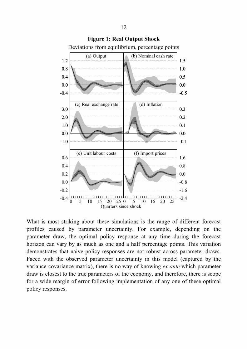
For example, consider a one percentage point shock to real output. Figure 1summarises the results of this simulation. In this figure, the maximum, minimumand median along with the first and third quartiles illustrate the dispersion offorecast profiles generated by the different parameter draws. The central black linedenotes the median, while the limits of the light shaded regions are the maximumand minimum. The darker shaded region corresponds to the inter-quartile range.

Note that the spread of forecasts around the median need not be symmetric. This isbecause asymmetries result from non-linearities in the way that the modelparameters enter the construction of the forecasts. Although the model is linear ineach of the variables, forecasts can be high-order polynomials in the lagcoefficients.

To begin with, the output shock opens up a positive output gap which generateswage pressures in the economy. Feedback between wages and prices means thatthis wage pressure eventually feeds into price inflation. Consistent with themonetary authority’s objectives, the optimal response to this shock is to initiallyraise the nominal cash rate. However, the size of this initial tightening can vary byup to three-quarters of a percentage point, depending on the parameter draw. Withbackward-looking inflation expectations, the rise in nominal interest rates raisesthe real cash rate, which has a dampening effect on output and eventually reversesthe upward pressure on unit labour costs and inflation. The higher real interest ratealso appreciates the real and nominal exchange rate, lowering inflation directly byreducing the Australian dollar price of imports and indirectly, by reducing outputgrowth.

Over time, the initial tightening is reversed and eventually policy follows adampening cycle as the output gap is gradually closed and wage and priceinflation pressures subside. In the limit, all real variables and growth rates returnto target and the system returns to the steady state.10

10 While this is true for the model which we are using in this paper, after the 27 periods shown in

Figure 1, some of the variables do not completely return to steady state. This is because themean parameter draw results in a model which is quite persistent anyway and furthermore,some of the more extreme parameter draws can generate larger and more long-lasting cyclicalbehaviour in the variables. Eventually, however, all of the real variables and growth rates willreturn to steady state.

12

Figure 1: Real Output ShockDeviations from equilibrium, percentage points

-2.4

-1.6

-0.8

0.0

0.8

1.6

-0.4

-0.2

0.0

0.2

0.4

0.6

-1.0

0.0

1.0

2.0

3.0

-1.0

0.0

1.0

2.0

3.0

-0.1

0.0

0.1

0.2

0.3

-0.1

0.0

0.1

0.2

0.3

-0.4

0.0

0.4

0.8

1.2

-0.4

0.0

0.4

0.8

1.2

-0.5

0.0

0.5

1.0

1.5

-0.5

0.0

0.5

1.0

1.5

(e) Unit labour costs

Quarters since shock

(f) Import prices

(c) Real exchange rate (d) Inflation

(a) Output (b) Nominal cash rate

2520151050 2520151050

What is most striking about these simulations is the range of different forecastprofiles caused by parameter uncertainty. For example, depending on theparameter draw, the optimal policy response at any time during the forecasthorizon can vary by as much as one and a half percentage points. This variationdemonstrates that naive policy responses are not robust across parameter draws.Faced with the observed parameter uncertainty in this model (captured by thevariance-covariance matrix), there is no way of knowing ex ante which parameterdraw is closest to the true parameters of the economy, and therefore, there is scopefor a wide margin of error following implementation of any one of these optimalpolicy responses.

13

It should be stressed that the optimal policy responses in Figure 1 assume nolearning on the part of the monetary authority. Although the monetary authoritymay set interest rates according to a calculated optimal policy path, the economywill only ever evolve according to the true parameter draw. Generically, theforecasts of the monetary authority will be proved wrong ex-post, providing asignal that the initial parameter estimates were incorrect. If the monetary authoritylearns more about the true model parameters from this signal, then Brainard-typeuncertainty will gradually become less relevant over time.11 However, in the naivepolicy responses shown in Figure 1, this type of learning is ruled out because weassume that the policy-maker always believes that the given parameter estimatesare the true parameter values. In this case, any deviation between the actual andforecast behaviour of the economy would be attributed to unanticipated shocks.

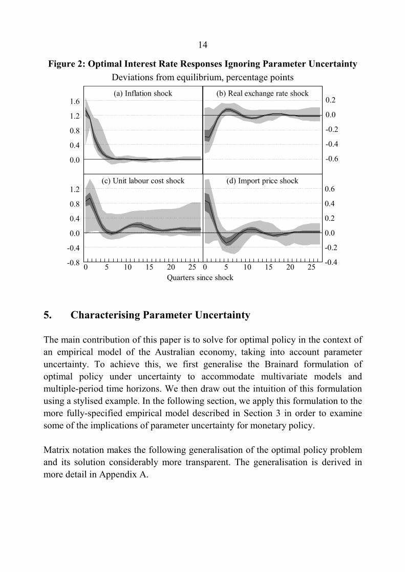
We also examine the range of forecast profiles obtained under shocks to the otherendogenous variables. Figure 2 shows the optimal response of the nominal cashrate to various other one percentage point shocks. These simulations are similar tothat shown for the output shock in the sense that they all exhibit considerablevariation in the optimal policy response across different parameter draws.However, in all cases, the optimal policy response drives the economy back intoequilibrium with real variables trending back to their baseline values and nominalgrowth rates stabilising in accordance with the inflation target.

These simulations show that, where there is uncertainty regarding the true modelparameters, the naive optimal policy response can vary quite considerably withobserved parameter estimates. There are certainly considerable risks involved inimplementing policy assuming that the estimated parameters are equal to their truevalues. In the next section, we demonstrate how the optimal policy problem can bemodified to explicitly take into account parameter uncertainty. Rather than solvingfor the optimal path of the cash rate for a particular set of parameter estimates, themonetary authority takes into account the uncertainty associated with thedistribution of parameter estimates and adjusts the policy response accordingly.

11 Of course, the policy-maker will not be able to resolve uncertainty through time if the source

of the ex-post forecasting error is parameter variation.

14

Figure 2: Optimal Interest Rate Responses Ignoring Parameter UncertaintyDeviations from equilibrium, percentage points

-0.8

-0.4

0.0

0.4

0.8

1.2

-0.4

-0.2

0.0

0.2

0.4

0.6

-0.6

-0.4

-0.2

0.0

0.2(b) Real exchange rate shock

(c) Unit labour cost shock (d) Import price shock

0.0

0.4

0.8

1.2

1.6(a) Inflation shock

Quarters since shock2520151050 2520151050

5. Characterising Parameter Uncertainty

The main contribution of this paper is to solve for optimal policy in the context ofan empirical model of the Australian economy, taking into account parameteruncertainty. To achieve this, we first generalise the Brainard formulation ofoptimal policy under uncertainty to accommodate multivariate models andmultiple-period time horizons. We then draw out the intuition of this formulationusing a stylised example. In the following section, we apply this formulation to themore fully-specified empirical model described in Section 3 in order to examinesome of the implications of parameter uncertainty for monetary policy.

Matrix notation makes the following generalisation of the optimal policy problemand its solution considerably more transparent. The generalisation is derived inmore detail in Appendix A.

15

The optimal policy problem for a monetary authority with quadratic preferencesgiven by Equation (1) and a backward-looking multivariate model of the economy(that is linear in both the variables and shocks) can be written in the followinggeneral form:

[ ]ΩTTR

′= ELossmin , (2)

subject to:

GRFT += , (3)

where T is a vector of policy targets in each period of the forecast horizon; R isthe vector of policy instruments; the matrices, F and G are functions of bothhistory and the parameter estimates while Ω summarises the penalties containedin the objective function. The time subscript has been omitted for simplicity. Thisgeneral form for the optimal policy problem highlights its similarity to theproblem originally solved by Brainard. Because the loss function is quadratic andthe constraint set is linear, the usual optimal policy response under parameteruncertainty will apply.

Specifically, if F and G are stochastic, then the solution to the optimal policyproblem is:

[ ] ,)()(~ 1 GΩFFΩFR* ′′−= − EE (4)

which can also be expressed as:

( ) ( ) ( ) ( ) ,~ 1

−′−+′

−′−+′−=

−

GGΩFFGΩFFFΩFFFΩFR* EE (5)

where F is the expectation of F and G is the expectation of G .

Alternatively, if F and G are deterministic (with values F and G ), then thesolution to the problem becomes:

( ) .1 GΩFFΩFR* ′′−= − (6)

16

F and G will be stochastic if they contain parameter estimates. Therefore, thesolution described by Equations (4) and (5) corresponds to optimal policyacknowledging parameter uncertainty. The deterministic case in Equation (6)describes the naive policy response, when the monetary authority ignoresparameter uncertainty. Comparing Equations (5) and (6), the difference betweenoptimal policy responses with and without parameter uncertainty can be ascribedto the variance of F and the covariance between F and G . Brainard’s policyconservatism result depends crucially on the independence of F and G . However,F and G will not be independent if they are derived from a model that exhibitspersistence.

To make the optimal-policy definition in Equation (5) operational, it is necessaryto compute the variance and covariance terms. This can be done using a sampleestimate of the loss function in Equation (2):

=

′=N

iiiN

Loss1

1 TΩT , (7)

where N is the number of parameter draws. This essentially computes the averageloss over N parameter draws. The first-order necessary condition for this lossfunction to be minimised subject to the set of constraints in Equation (3) is thenjust the sample estimate of (4):

.11ˆ1

1

1

′

′−= =

−

=

N

iii

N

iii NN

GΩFFΩFR* (8)

By averaging across a large number of parameter draws, optimal policy can becomputed from the linear relationship between the target variables of policy andthe policy instrument. As the number of draws from the estimated parameterdistribution increases, this approximation will tend to the true optimal policy givenby Equation (4). The naive policy response is computed by setting N=1 and usingthe mean parameter draw to compute optimal policy from Equation (8). In thiscase, the mean parameter draw is interpreted as the ‘true’ model parameters,ignoring any uncertainty which we may have about them.

17

To illustrate the intuition behind these results, we first examine optimal policyresponses in a stylised model which is an extension of the model considered byBrainard (1967). In the next section, we apply the generalised optimal policysolution to the model summarised in Table 1.

The original Brainard model assumed that the policy-maker minimised squareddeviations of a variable y from a target (normalised to zero) by controlling a singlepolicy instrument i, for an economy described by:

ttt iy εθ += , (9)

where θ is an unknown parameter representing the effectiveness of policy and εis an independently and identically distributed white-noise process. To explore theissues involved in generalising this specification, it is useful to consider aneconomy that also includes a role for dynamics:

tttt yiy ερθ ++= −1 , (10)

where ρ is another unknown parameter representing the degree of persistence inthe economy.

In this model, parameter uncertainty arises when ρ and θ can only be impreciselyestimated. The central message of this section and the next is that the implicationsof parameter uncertainty depend crucially upon the relative uncertainty aboutpolicy effectiveness (θ ) and persistence ( ρ ). If uncertainty about policyeffectiveness dominates, then the usual Brainard conservatism result obtains.However, if uncertainty about persistence is more important, then optimal policymay be more aggressive.

The loss function is assumed to be the unweighted sum of squared deviations ofthe target variable y in the current and all future periods. For a given shock to thetarget variable, the optimal policy response is found by minimising this lossfunction. Assume that the two parameter estimates in Equation (10) are drawnfrom different independent normal distributions. For the uncertainty-awareoptimal policy, we take one thousand draws from the underlying parameterdistributions and compute the optimal policy response using the frequencysampling approach described by Equation (8). We then compare this with the

18

naive optimal policy response which is computed using only the mean parameterdraw.

To contrast the policy implications of each of these two types of uncertainty, wederive the optimal policy responses to a standardised shock under differing levelsof relative uncertainty about each of the parameters. In what follows, we assumethat there is a one unit shock to the target variable in the initial period ( 10 =ε ), butthereafter ε is zero.

First, we examine the case where the persistence parameter is known withcertainty, but the policy effectiveness parameter can only be estimatedimprecisely.12 Figure 3(a) shows that the uncertainty-aware optimal policyresponse to the shock in y is more conservative than the naive response.Consequently, using the mean parameter draw to forecast the target variableoutcomes in Figure 3(b), the uncertainty-aware policy response means that thetarget variable takes longer to return to target. Of course, the actual ex-postoutcome under both policy responses will depend upon the ‘true’ parameters,which need not coincide with the mean parameter draw.

12 Specifically, in this simulation we assume that the persistence parameter ρ takes the value

0.5 with certainty while the policy effectiveness parameter θ is drawn from a normaldistribution with mean –0.5 and variance 0.25.

19

Figure 3: Uncertainty about Policy Effectiveness

-0.3 -0.2 -0.1 0.0 0.1 0.2 0.30

30

60

90

120

150

180

210

240

270(a) Optimal policy responses

(Two periods after the shock)

Periods since shock

Naive

0.0

0.3

0.6

0.9

1.2

0.0

0.3

0.6

0.9

1.2

-1 0 1 2 3 4-0.3

0.0

0.3

0.6

0.9(b) Target variable outcomes

(c) Histogram of target variableoutcomes

Uncertainty-aware

Naive

Uncertainty-aware

Uncertainty-aware policyNaive policy

For the two instrument paths shown in Figure 3(a), we can derive the impliedex-post target variable outcomes at any time horizon for each of the one thousandparameter draws. From this, we derive the distribution of target variable outcomes,which is presented as a histogram in Figure 3(c). In this Figure we only show thedistribution of target variable outcomes two periods after the shock. As expected,under naive policy, the distribution of outcomes is approximately normallydistributed with mean zero. For the conservative, uncertainty-aware optimalpolicy, however, the distribution of target variable outcomes for the one thousandparameter draws is slightly skewed and more tightly focused on small positiveoutcomes. In this example, because the conservative policy response reduces thespread of possible outcomes, it will generate a lower expected sum of squareddeviations of y from target and dominates the naive policy response. This, ofcourse, echoes Brainard’s result; when there is uncertainty about the effects ofpolicy then it pays to be more conservative with the policy instrument because thelarger the change in the instrument, the greater will be the uncertainty about itsfinal effect on the economy.

20

At the other extreme, we now consider the case where the effectiveness of policyis known with certainty, but the degree of persistence can only be impreciselyestimated.13 Using the same one thousand parameter draws as before, the results inFigure 4(a) suggest that the uncertainty-aware optimal policy response is nowmore aggressive than the naive policy response. Figure 4(b) shows the targetvariable outcomes for these two policy responses using the mean parameter draw.

Figure 4: Uncertainty about Persistence

0.0

0.3

0.6

0.9

1.2

0.0

0.3

0.6

0.9

1.2

-0.1 0.0 0.1 0.2 0.3 0.4 0.50

50

100

150

200

250

300

350

400

450(a) Optimal policy responses

(Two periods after the shock)

Periods since shock

Naive

-1 0 1 2 3 4-0.3

0.0

0.3

0.6

0.9(b) Target variable outcomes

(c) Histogram of target variableoutcomes

Uncertainty-aware

Naive

Uncertainty-aware

Uncertainty-aware policyNaive policy

If the policy-maker ignores uncertainty, then the target variable will only followthe path shown in Figure 4(b) if the ‘true’ parameters coincide with the meanparameter draw. The target variable will overshoot, however, if persistence islower than expected.14 In this case, because the economy is less persistent than

13 In this case, θ takes the value –0.5 with certainty and ρ is drawn from a normal distribution

with mean 0.5 and variance 0.25.14 Here an overshooting is defined as a negative target variable outcome because the initial

shock was positive. An undershooting, then, is defined as a positive target variable outcome.

21

expected, the overshooting will be rapidly unwound, meaning that the shock isless likely to have a lasting impact on the economy. In contrast, if the targetvariable undershoots, then persistence must be higher than expected, so the effectof the shock will take longer to dissipate. A policy-maker that is aware ofparameter uncertainty will take this asymmetry into account, moving the policyinstrument more aggressively in response to a shock.15 This will ensure that morepersistent outcomes are closer to target at the cost of forcing less persistentoutcomes further from target. This reduces the expected losses because theoutcomes furthest from target unwind most quickly.

Generally speaking, when there is uncertainty about how persistent the economyis, that is, how a shock to y will feed into future values of y, then it makes sense tobe more aggressive with the policy instrument with the hope of minimisingdeviations of the target variable as soon as possible. In Figure 4(c), for example,the aggressive uncertainty-aware policy response reduces the likelihood ofundershooting, at the cost of increasing the chance of overshooting. This policyresponse dominates, however, because the loss sustained by the many smallnegative outcomes that it induces is more than offset by the greater loss sustainedby the large positive outcomes associated with naive policy.16

These two simple examples show that the implications of parameter uncertaintyare ambiguous. Policy should be more conservative when the effectiveness ofpolicy is relatively imprecisely estimated, while policy may be more aggressivewhen the persistence of the economy is less precisely estimated. In between thetwo extreme examples which we have considered here, when there is uncertaintyabout all or most of the coefficients in a model, then one cannot conclude a prioriwhat this entails for the appropriate interest-rate response to a particular shock. Inthe context of any estimated model, it remains an empirical issue to determine theimplications of parameter uncertainty for monetary policy. This is what we do inthe next section.

15 Of course, there is a limit on how aggressive policy can be before it causes worse outcomes.16 However, in this case, it is important to recognise that if the loss function contained a discount

factor then this could reduce the costs of conservative policy. For example, with discounting,the naive policy-maker in Figure 4 will be less concerned about bigger actual losses sustainedfurther into the forecast horizon. This result applies more generally; if policy-makers do notcare as much about the future as the present, then they may prefer less activism rather thanmore.

22

This example also highlights the importance of assuming that monetary authoritiesnever learn about the true model parameters. The monetary authority alwaysobserves the outcome in each period of time. If the extent of the policy error in thefirst period conveys the true value of ρ or θ , then policy could be adjusted todrive y to zero in the next period. Ruling out learning prevents these ex-postpolicy adjustments, making the initial policy stance time consistent. To the extentthat uncertainty is not being resolved through time, this is a relevant description ofpolicy. Additional data may sharpen parameter estimates but these gains are oftenoffset by instability in the underlying parameters themselves. Sack (1997)explored the case in which uncertainty about the effect of monetary policy isgradually resolved through time by learning using a simple model in which theunderlying parameters are initially chosen from a stochastic distribution.

6. Optimal Policy Acknowledging Parameter Uncertainty

In this section we present uncertainty-aware optimal policy computations for themodel described in Section 3 and compare them with naive optimal policyresponses. The uncertainty-aware optimal policy response computed fromEquation (8) is estimated using one thousand different draws from the underlyingparameter distribution. A large number of draws is required because of the largenumber of parameters.

When computing the naive optimal policy response, it is necessary to specify theparameter vector that the monetary authority interprets as being the ‘true’parameter values. Usually this vector would contain the original parameterestimates. However, we compute the naive policy response using the averagevalue of the parameter vector draws. This prevents differences between the twopolicy profiles being driven by the finite number of parameter draws, the averageof which may not coincide exactly with the original parameter draw.

Beginning with a one percentage point shock to output, Figure 5(a) comparesoptimal policy responses using the model described in Section 3. The darker linerepresents optimal policy when parameter uncertainty is taken into account whilethe lighter line represents the naive optimal policy response.

23

Figure 5: Optimal Interest Rate Responses Ignoring andAcknowledging Parameter Uncertainty

Deviations from equilibrium, percentage points

0 5 10 15 20 25-0.4

0.0

0.4

0.8

1.2

0 5 10 15 20 25-0.4

0.0

0.4

0.8

1.2

-0.2

-0.1

0.0

0.1

-0.2

-0.1

0.0

0.1

-0.2

0.0

0.2

0.4

-0.2

0.0

0.2

0.4

-0.5

0.0

0.5

1.0

1.5

-0.5

0.0

0.5

1.0

1.5(a) Real output shock

Quarters since shock

Acknowledginguncertainty

Ignoringuncertainty

(b) Real exchange rateshock

(c) Import price shock

(d) Inflation shock (e) Unit labour costshock

The key feature of interest in Figure 5(a) is the larger initial policy response whenuncertainty is taken into account. While later oscillations in the cash rate aresimilar in magnitude, the early response of the cash rate is somewhat larger whenpolicy takes parameter uncertainty into account. The finding that policy shouldreact more aggressively because of parameter uncertainty is specific to the outputshock used to generate Figure 5(a). For example, the naive policy response isrelatively more aggressive for a one percentage point shock to the real exchangerate, as shown in Figure 5(b). This suggests that the persistence of a real exchangerate shock is more precisely estimated than the persistence of an output shockrelative to the estimated effectiveness of policy for each of these shocks. With lessrelative uncertainty about the persistence of a real exchange rate shock, the

24

optimal policy response taking into account uncertainty is more conservativebecause it is dominated by uncertainty about policy effectiveness.

Figures 5(c) - 5(e) present the policy responses to shocks to import prices,consumer prices and unit labour costs respectively. In each case, the naive policyresponse is initially more conservative than the policy response which takesaccount of parameter uncertainty.

These three types of nominal shocks to the model confirm that conservatism is byno means the generic implication of parameter uncertainty. In our model, itappears that uncertainty about the effectiveness of the policy instrument isgenerally dominated by uncertainty about model persistence and this explains themore aggressive optimal policy response to most of the shocks which weexamined.

7. Conclusion

This paper extends Brainard’s formulation of policy-making under uncertainty inseveral directions. First, it generalises the solution of the optimal policy problemto accommodate multiple time-periods and multiple objectives for policy. Thisgeneralisation develops the stochastic properties of the equations relating targetvariables to the policy instrument from the estimated relationships defining theunderlying economic model.

Whereas uncertainty about the effectiveness of monetary policy tends torecommend more conservative policy, we explore the intuition for why otherforms of parameter uncertainty may actually lead to more aggressive policy. In asimple example, we show that uncertainty about the dynamics of an economy canbe a source of additional policy activism. However, this consequence of parameteruncertainty is only relevant in a multi-period generalisation of the Brainard model.

25

In the context of any specific model, it is an empirical issue to determine the exactimplications of parameter uncertainty for monetary policy. We examine this usinga small linear model of the Australian economy that captures the key channels ofthe monetary policy transmission mechanism within an open-economy framework.Optimal policy responses ignoring parameter uncertainty are compared withoptimal responses that explicitly take parameter uncertainty into account. Whilethe differences between these policy responses vary with the source of shocks tothe economy, our evidence suggests that, for most shocks in our model, parameteruncertainty motivates somewhat more aggressive use of the instrument.

Although the results in this paper are reported as deviations from equilibrium, themethod used to construct optimal policy responses under parameter uncertainty isalso applicable in a forecasting environment where past data must be taken intoaccount. The approach is applicable to all backward-looking linear models inwhich the objectives of the policy-maker are quadratic.

The simulations also demonstrate how frequency-sampling techniques can be usedto evaluate the analytic expression for optimal policy under parameter uncertainty,despite the presence of complex expectations terms. This approach to policydetermination is as practical, and more theoretically appealing, than theapplication of alternative rules-based approaches.

While the findings of the paper are of considerable interest, they should not beoverstated. In particular, the implications of parameter uncertainty are dependentupon the type of shock being accommodated. They are also dependent upon thespecification of the model. For example, changes to the model specification couldsubstantially alter the measured uncertainty attached to the effectiveness of policyrelative to the measured uncertainty associated with the model’s dynamics. If thetechniques developed in this paper are to be of wider use, the underlying modelmust first be well understood and carefully specified. Also, it is worthremembering that, although our model suggests that optimal monetary policytaking account of uncertainty is more activist for most kinds of shocks, thedifference in policy response is quite small relative to the degree of conservatismthat is actually practiced by most central banks.

26

In this paper we have not sought to argue that conservative monetary policy is notoptimal. In fact, there are probably a number of good reasons why conservativepolicy may be optimal. Instead, the central message of the paper is that, if we areto motivate conservative monetary policy, then explanations other than Brainard’sare required.

27

Appendix A: Generalising the Optimal Policy Problem

In this appendix, we generalise Brainard’s (1967) solution to the optimal policyproblem for a monetary authority with quadratic preferences using a dynamic,multivariate model with stochastic parameter uncertainty.

To begin with, we show how the optimal policy problem for a monetary authoritywith quadratic preferences given by Equation (1) and a backward-lookingmultivariate model of the economy (that is linear in both the variables and theshocks) can be written in the following general form:

[ ]TΩTR

′= ELossmin , (A1)

subject to:GRFT += . (A2)

To prove this, recall that the preferences of the monetary authority can besummarised by the following intertemporal quadratic loss function:

−+−+=

= =−+++

=+

h

j

h

jjtjtjt

h

jjtt iigapELoss

1 1

21

2*

1

2 )()( γππβα , (A3)

which can be rewritten using matrix notation as:

[ ]tttttttELoss RΓIΓIRΠΠYY )()( −′−′−′+′= γβα (A4)

where:

[ ] ′= +++ htttt gapgapgap 21Y , (A5)

( ) ( ) ( )[ ] ′−−−= +++**

2*

1 ππππππ htttt Π , (A6)

[ ] ′= +++ htttt iii 21R , (A7)

28

Γ is the matrix that lags the nominal interest rate vector tR by one period; and Iis an ( hh× ) identity matrix. The subscript t denotes the current date from whichforecasts are being generated.

Given that the model of the economy (Table 1) is linear, the policy target variablesare affine transformations of the forecast profile for the policy instrument:

BRAY += tt (A8)

and

DRCΠ += tt , (A9)

where A , B , C and D are stochastic matrices constructed from the parameters ofthe model and the history of the economy. The structure of these stochasticmatrices is determined by the relationships laid out in the definition of the model’sequations. Matrices B and D are the impulse response functions of the output gapand inflation to a shock at time t. Likewise, matrices A and C are the marginalimpact of the nominal cash rate on the output gap and inflation respectively.

By defining tt RΓΙ∆ )( −≡ as the vector of first differences in the nominal cashrate over the forecast horizon, it is possible to specify the full set of policy targetsas:

[ ]tttt ∆ΠYT ′′′= . (A10)

Then, upon dropping time subscripts, the optimal policy problem can be restatedsuccinctly as:

[ ]TΩTR

′= ELossmin , (A11)

subject to:GRFT += , (A12)

where the matrices F and G are defined in terms of A , B , C , D and )( ΓΙ − as:

29

=

−=

0

000000

DB

G

ΓΙC

AF

(A13)

and the weights on the different components of the loss function α , β and γ ,have been subsumed into the diagonal matrix Ω according to:

ΙΩ ⊗

=γ

βα

000000

(A14)

where I is the same identity matrix used to define the first differences in the cashrates, ∆ . Ignoring the fact that it is in matrix notation and observing that the targetvalues of the target variables have been normalised to zero, this problem is exactlythe same as that examined by Brainard (1967).

If F and G are stochastic, the solution to the optimal policy problem described byEquations (A1) and (A2) is:

[ ] ,)()(~ 1 GΩFFΩFR* ′′−= − EE (A15)

which can also be expressed as:

( ) ( ) ( ) ( ) .~ 1

−′−+′

−′−+′−=

−

GGΩFFGΩFFFΩFFFΩFR* EE (A16)

Alternatively, if F and G are deterministic (with values F and G ), then thesolution to the optimal policy problem is:

( ) .1 GΩFFΩFR* ′′−= − (A17)

30

To show this, rewrite the loss function in Equation (A1) by adding and subtractingthe expected values of T from it, yielding:

[ ])()(min ′+−′+−= TTTΩTTTR

ELoss . (A18)

Upon expanding, this loss function can be also be expressed as:

[ ] [ ][ ] ,)()(

2)()(min

TΩTTTΩTT

TTΩTTΩTTTΩTTR

′+−′−=

−′+′+−′−=

E

EELoss(A19)

taking advantage of the fact that TT ≡)(E .

Substituting in Equation (A2) and simplifying then yields:

[ ].

(())((min

GΩGGΩFR2

RFΩFRGGR)FFΩGGRFFR

′+′′+

′′+−+−′−+−= ELoss(A20)

The first order necessary condition for this optimisation problem is obtained bydifferentiating with respect to R :

02~2~)()(2~)()(2 =′+′+−′−+−′− GΩFRFΩFRGGΩFFRFFΩFF *** .(A21)

Solving for *R~ then gives optimal policy when taking uncertainty into account, asexpressed in Equations (A15) and (A16). Given that the loss function is strictlyconvex, this first order necessary condition is also sufficient for a minimum of theexpected loss function.

The naive optimal policy response shown in Equation (A17) obtains as asimplification of Equation (A16) when F is set to F and G is set to G , that is,when F and G are deterministic.

31

References

Blinder, A.S. (1995), ‘Central Banking in Theory and Practice: Lecture 1:Targets, Instruments and Stabilization’, Marshall Lecture, presented at theUniversity of Cambridge, Cambridge, UK.

Brainard, W. (1967), ‘Uncertainty and the Effectiveness of Policy’, AmericanEconomic Review, 57(2), pp. 411–425.

Clements, M.P. and D.F. Hendry (1993), ‘On the Limitations of ComparingMean Square Forecast Errors’, Journal of Forecasting, 12(8), pp. 617–637.

Clements, M.P. and D.F. Hendry (1994), ‘Towards a Theory of EconomicForecasting’, in C. Hargreaves (ed.), Non-stationary Time-series Analysis andCointegration, Oxford University Press, Oxford, pp. 9–52.

Clements, M.P. and D.F. Hendry (1996), ‘Intercept Corrections and StructuralChange’, Journal of Applied Econometrics, 11(5), pp. 475–494.

de Brouwer, G. and L. Ellis (1998), ‘Forward-looking Behaviour andCredibility: Some Evidence and Implications for Policy’, Reserve Bank ofAustralia Research Discussion Paper No. 9803.

Epstein, L.G. and T. Wang (1994), ‘Intertemporal Asset Pricing UnderKnightian Uncertainty’, Econometrica, 62(2), pp. 283–322.

Harvey, A.C. (1989), Forecasting, Structural Time Series Models and the KalmanFilter, Cambridge University Press, Cambridge.

Knight, F.H. (1921), Risk, Uncertainty and Profit, Houghton Mifflin Co., Boston.

Kremers, J.M., N.R. Ericsson and J.J. Dolado (1992), ‘The Power ofCointegration Tests’, Oxford Bulletin of Economics and Statistics, 54(3), pp.325-348.

32

Kwakernaak, H. and R. Sivan (1972), Linear Optimal Control Systems, Wiley,New York.

Lowe, P. and L. Ellis (1997), ‘The Smoothing of Official Interest Rates’, inP. Lowe (ed.), Monetary Policy and Inflation Targeting, Reserve Bank ofAustralia, Sydney, pp. 286–312.

Orphanides, A. (1998), ‘Monetary Policy Evaluation with Noisy Information’,Federal Reserve System Finance and Economics Discussion Paper No. 1998/50.

Sack, B. (1997), ‘Uncertainty and Gradual Monetary Policy’, MassachusettsInstitute of Technology, mimeo.