The Impacts of the Clean Air Act Amendments of 1990and Changes in Rail Rates on Western Coal

by

John BitzanDenver Tolliver

Wayne Linderman

Upper Great Plains Transportation InstituteNorth Dakota State University

Fargo, North Dakota

April 1996

Disclaimer

The contents of this report reflect the views of the authors, who are responsible for the facts and theaccuracy of the information presented herein. This document is disseminated under the sponsorship of theDepartment of Transportation, University Transportation Centers Program, in the interest of informationexchange. The U.S. Government assumes no liability for the contents or use thereof.

ABSTRACT

This study examines the impacts of the Clean Air Act Amendments of 1990 (CAAA90) on

coal production and coal flows. The CAAA90 take a markedly different approach to pollution control

from stationary sources when compared to past `clean air' legislation. The new approach to limiting

sulfur dioxide emissions from electric utilities allows the least cost method of pollution control to be used

by those utilities that realize the lowest costs in reducing pollution. In many cases, the lowest cost

method of reducing pollution will be to purchase low sulfur coal. Because 86 percent of the nation's

recoverable low sulfur coal reserves are located in the west, this presents a great opportunity for

western coal producers. Linear programs are estimated in the study, showing the large potential

increases in western coal production resulting from the CAAA90. Finally, the study shows that future

changes in nationwide transportation rates could have a major impact on regional coal production and

market shares. To the extent that increases in railroad efficiency continue, western coal production

should realize an even greater opportunity. This study also presents a model of rail rates, showing the

influences of costs and competitive factors in determining individual rates for coal.

i

TABLE OF CONTENTS

INTRODUCTION . . . . . . . . . . . . . . . . . . . . . . . . . . . . . . . . . . . . . . . . . . . . . . . . . . . . . . . . . . . . . . . 1Coal Quality . . . . . . . . . . . . . . . . . . . . . . . . . . . . . . . . . . . . . . . . . . . . . . . . . . . . . . . . . . . . . 3Coal Origin Regions . . . . . . . . . . . . . . . . . . . . . . . . . . . . . . . . . . . . . . . . . . . . . . . . . . . . . . . . 5Coal Production . . . . . . . . . . . . . . . . . . . . . . . . . . . . . . . . . . . . . . . . . . . . . . . . . . . . . . . . . . . 8Coal Consumption . . . . . . . . . . . . . . . . . . . . . . . . . . . . . . . . . . . . . . . . . . . . . . . . . . . . . . . . 10Electricity Demand Regions . . . . . . . . . . . . . . . . . . . . . . . . . . . . . . . . . . . . . . . . . . . . . . . . . 13

East North Central Region . . . . . . . . . . . . . . . . . . . . . . . . . . . . . . . . . . . . . . . . . . . . . 16West South Central Region . . . . . . . . . . . . . . . . . . . . . . . . . . . . . . . . . . . . . . . . . . . . 19South Atlantic Region . . . . . . . . . . . . . . . . . . . . . . . . . . . . . . . . . . . . . . . . . . . . . . . . 21West North Central Region . . . . . . . . . . . . . . . . . . . . . . . . . . . . . . . . . . . . . . . . . . . . 23Mountain Region . . . . . . . . . . . . . . . . . . . . . . . . . . . . . . . . . . . . . . . . . . . . . . . . . . . 25

Coal Transportation . . . . . . . . . . . . . . . . . . . . . . . . . . . . . . . . . . . . . . . . . . . . . . . . . . . . . . . 26Rail Transportation of Western Coal . . . . . . . . . . . . . . . . . . . . . . . . . . . . . . . . . . . . . . . . . . . . 30

THE CLEAN AIR ACT AMENDMENTS OF 1990 . . . . . . . . . . . . . . . . . . . . . . . . . . . . . . . . . . . . . . . 33Rail Rates for Coal Transport . . . . . . . . . . . . . . . . . . . . . . . . . . . . . . . . . . . . . . . . . . . . . . . . 39

Determinants of Variations in Rail Coal Rates . . . . . . . . . . . . . . . . . . . . . . . . . . . . . . . 42Data . . . . . . . . . . . . . . . . . . . . . . . . . . . . . . . . . . . . . . . . . . . . . . . . . . . . . . . . . . . . 46Estimation Results . . . . . . . . . . . . . . . . . . . . . . . . . . . . . . . . . . . . . . . . . . . . . . . . . . 47

The Impact of the Clean Air Act Amendments on Western Coal . . . . . . . . . . . . . . . . . . . . . . . . 50Data Used for the Linear Programs . . . . . . . . . . . . . . . . . . . . . . . . . . . . . . . . . . . . . . 57Model and Data Issues . . . . . . . . . . . . . . . . . . . . . . . . . . . . . . . . . . . . . . . . . . . . . . . 62Base Model Results . . . . . . . . . . . . . . . . . . . . . . . . . . . . . . . . . . . . . . . . . . . . . . . . . 63

CONCLUSION . . . . . . . . . . . . . . . . . . . . . . . . . . . . . . . . . . . . . . . . . . . . . . . . . . . . . . . . . . . . . . . . 78

REFERENCES . . . . . . . . . . . . . . . . . . . . . . . . . . . . . . . . . . . . . . . . . . . . . . . . . . . . . . . . . . . . . . . . 81

APPENDIX - SUPPLEMENTARY TABLES . . . . . . . . . . . . . . . . . . . . . . . . . . . . . . . . . . . . . . . . . . . . 83

ii

LIST OF FIGURES

Figure 1. Coal-Bearing Areas of the United States . . . . . . . . . . . . . . . . . . . . . . . . . . . . . . . . . . . . 6Figure 2. U.S. Coal Production and Purchases, 1991 . . . . . . . . . . . . . . . . . . . . . . . . . . . . . . . . . . 9Figure 3. U.S. Coal Production and Purchases, 1980-91 . . . . . . . . . . . . . . . . . . . . . . . . . . . . 10Figure 4. Distribution of Coal Produced in the U.S., 1991 . . . . . . . . . . . . . . . . . . . . . . . . . . . . . 11Figure 5. U.S. Coal Distribution, 1991 (By Region) . . . . . . . . . . . . . . . . . . . . . . . . . . . . . . . . . . 12Figure 6. Percent of Coal Shipped to Electric Utilities . . . . . . . . . . . . . . . . . . . . . . . . . . . . . . . . 13Figure 7. Census Divisions . . . . . . . . . . . . . . . . . . . . . . . . . . . . . . . . . . . . . . . . . . . . . . . . . . . 14Figure 8. U.S. Electric Utility Receipts of Coal, 1991 . . . . . . . . . . . . . . . . . . . . . . . . . . . . . . . . . 15Figure 9. Receipts of Coal by Electric Utilities in Major Demand Regions, 1980-91 . . . . . . . . . . . . 16Figure 10. Coal Received by Electric Utilities in the East North Central Region, 1991 . . . . . . . . . . . 17Figure 11. Coal Delivered to Electric Utilities in the East North Central Region, 1980-91 . . . . . . . . . 18Figure 12. Coal Received by Electric Utilities in the West South Central Region, 1991 . . . . . . . . . . . 19Figure 13. Coal Delivered to Electric Utilities in the West South Central Region, 1980-91 . . . . . . . . 20Figure 14. Coal Received by Electric Utilities in the South Atlantic Region, 1991 . . . . . . . . . . . . . . 21Figure 15. Coal Delivered to Electric Utilities in the South Atlantic Region, 1980-91 . . . . . . . . . . . . 22Figure 16. Coal Received by Electric Utilities in the West North Central Region, 1991 . . . . . . . . . . 23Figure 17. Coal Delivered to Electric Utilities in the West North Central Region, 1980-91 . . . . . . . . 24Figure 18. Coal Received by Electric Utilities in the Mountain Region, 1991 . . . . . . . . . . . . . . . . . 25Figure 19. Transportation of Coal to Final Destination, 1991 . . . . . . . . . . . . . . . . . . . . . . . . . . 27Figure 20. Method of Transporting Coal to Final Desintation, 1991 . . . . . . . . . . . . . . . . . . . . . . . 28Figure 21. Percentage of U.S. Coal Shipments Delivered by Rail, 1980-91 . . . . . . . . . . . . . . . . . . . 29Figure 22. Coal as a Percentage of Revenue Freight Traffic and Total Revenue for

Class I Railroads . . . . . . . . . . . . . . . . . . . . . . . . . . . . . . . . . . . . . . . . . . . . . . . . . . . 30

iii

LIST OF TABLES

Table 1. Coal BTU Categories . . . . . . . . . . . . . . . . . . . . . . . . . . . . . . . . . . . . . . . . . . . . . . . . . 4Table 2. Coal Sulfur Content Categories . . . . . . . . . . . . . . . . . . . . . . . . . . . . . . . . . . . . . . . . . . 5Table 3. Coal Producing Regions of the United States . . . . . . . . . . . . . . . . . . . . . . . . . . . . . . . 5Table 4. Characteristics of Coal in the Three Producing Regions . . . . . . . . . . . . . . . . . . . . . . . . . 8Table 5. Estimation of Revenue per Ton Mile for Coal Rail Shipments . . . . . . . . . . . . . . . . . . . . 48Table 6. Data Sources for the Linear Programs . . . . . . . . . . . . . . . . . . . . . . . . . . . . . . . . . . . . 58Table 7. Estimation of In(CAPKW) . . . . . . . . . . . . . . . . . . . . . . . . . . . . . . . . . . . . . . . . . . . . 62Table 8. Coal Production Simulated by Minimizing Transport Costs with No Consideration

of Coal Sulfur Content . . . . . . . . . . . . . . . . . . . . . . . . . . . . . . . . . . . . . . . . . . . . . . . 64Table 9. Transportation as a Percentage of Total Acquisition Costs Based on Flows

Simulated by Minimizing Transport Costs with No Consideration ofSulfur Content . . . . . . . . . . . . . . . . . . . . . . . . . . . . . . . . . . . . . . . . . . . . . . . . . . . . 65

Table 10. Coal Production Simulated by Minimizing Transport Costs Subject to SulfurLimitations, with Current Rail Rates . . . . . . . . . . . . . . . . . . . . . . . . . . . . . . . . . . . . . 66

Table 11. Transportation as a Percentage of Total Acquisition Costs (does not include retrofitcosts) Based on Flows Simulated by Minimizing Transport Costs Subject to SulfurLimitations . . . . . . . . . . . . . . . . . . . . . . . . . . . . . . . . . . . . . . . . . . . . . . . . . . . . . . . 67

Table 12. Comparison of Coal Acquisition Costs for Utilities Between the Base Case and theSwitching Case (switching case includes retrofit costs) . . . . . . . . . . . . . . . . . . . . . . . . 68

Table 13. Coal Switching Simulated by the Impact Model That Does Not Allow ScrubberInstallation to Take Place . . . . . . . . . . . . . . . . . . . . . . . . . . . . . . . . . . . . . . . . . . . . . 70

Table 14. Coal Production Simulated by Minimizing Transport Costs Subject to SulfurLimitations, with a 10 Percent Overall Increase in Rail Rates . . . . . . . . . . . . . . . . . . . . . 72

Table 15. Coal Production Simulated by Minimizing Transport Costs Subject to SulfurLimitations, with a 10 Percent Overall Reduction in Rail Rates . . . . . . . . . . . . . . . . . . . 73

Table 16. New Scrubber Installations Simulated by the Impact Model That Does Not AllowFuel Switches . . . . . . . . . . . . . . . . . . . . . . . . . . . . . . . . . . . . . . . . . . . . . . . . . . . . . 74

Table 17. Comparison of Coal Acquisition Costs for Utilities Between the Base Case andthe Scrubber Retrofit Case (impact case includes scrubber retrofit costs) . . . . . . . . . . . 76

iv

1Alaska, Arizona, California, Colorado, Hawaii, Idaho, Montana, Nebraska, Nevada, New Mexico, NorthDakota, Oregon, South Dakota, Utah, Washington, and Wyoming.

2Smith, James N. And Robert R. Rose. Rail Transport of Western Coal. Prepared for the WesternGovernor’s Association, 1985.

3Energy Information Administration. Coal Production, 1990.

4Energy Information Administration. Annual Outlook for U.S. Electric Power, 1991.

1

INTRODUCTION

The market for western coal has grown immensely in recent years. This market growth is evident

in production trends. In states comprising the Western Governor's Association,1 there were 45 million tons

of coal produced in 1970.2 By 1991, annual production by these states had increased by more than 600

percent, reaching a level of more than 340 million tons.3 Much of this rise in the demand for western coal

has been a result of the increased desire for low sulfur coal by electric utilities in the United States.

Coal has been the dominant source of fuel used for generating electricity for many years, increasing its

share of electric energy generation from 46 percent in 1970, to 53 percent in 1990.4 Much of coal's

dominance in the electric utility market can be attributed to its status as the lowest-cost fossil fuel in terms

of price per BTU. Two characteristics of western coal that make its market potential great are low costs

of production and low sulfur content. First, the majority of western coal is produced in surface mines with

dense seams of coal that are easily accessible. This results in higher labor productivity, lower capital

costs, and a resulting lower cost associated with mining this coal. Second, the majority of western coal is

subbituminous coal which is generally low in sulfur. Nearly 95 percent of the recoverable reserves in the

west have less than 1.67 pounds of sulfur per million BTU, and 55 percent of the recoverable reserves in

the west have less than .6 pounds of sulfur per million BTU. By comparison, only 22 percent of the

Appalachian Region's recoverable reserves have less than .6 pounds of sulfur per million BTU, and less

than 1 percent of the Interior Region's recoverable reserves have less than.6 pounds of sulfur per million

2

BTU. More than 86 percent of the nation's low sulfur (less than .6 lbs. per million BTU) recoverable

reserves are located in the west.

There is currently a window of opportunity for western coal producers that previously has not existed.

Due to the Clean Air Act Amendments of 1990 (CAAA90), the demand for low sulfur coal is likely to

grow significantly in the next several years. The Amendments place strict limitations on the amount of

sulfur dioxide that may be emitted by electric utilities. However, they do not impose any requirements on

the geographic distribution of these emissions, or on how these emission limitations must be achieved.

Therefore, the least cost method of reducing sulfur dioxide emissions can be employed by those utilities

that experience the least costs in reducing such emissions. In many cases, this entails switching to low

sulfur coal.

One factor that may have a significant impact on the least cost method of reducing sulfur dioxide

emissions by utilities is the transportation rates for coal. While western coal is generally produced more

inexpensively than eastern coal, it faces a transportation disadvantage due to long distances to consuming

markets and lack of transportation competition.

This study examines opportunities associated with the Clean Air Act Amendments of 1990 (CAAA90),

and illustrates the impacts of various transportation rate changes on western coal production. By

understanding the potential opportunities associated with the Clean Air Act, western coal producers will

be better prepared to take advantage of such opportunities. An understanding of the dependence of coal

producing regions on the various modes of transportation will similarly allow producers to adjust to

changing conditions given a change in relative modal rates. The specific objectives of this study are as

follows:

1. Examine coal production, coal markets, and transportation trends over time.

3

2. Examine the Clean Air Act Amendments of 1990 and the opportunities they provide to

western coal producers.

3. Present a model of coal rail rates, showing how rail coal rates vary with intermodal,

intramodal, geographic, and product competition. These factors will be assessed in coal

producing regions and used to estimate western and eastern coal rail rates.

4. Present three spatial equilibrium models that show the optimal distribution of coal

nationwide. The first model will minimize the production and transportation costs of coal

shipped to electric utilities and will represent a base case. The second will minimize

production, transportation, and scrubbing costs, and place limitations on sulfur dioxide

emissions consistent with the Clean Air Act Amendments. This will estimate the impacts

of the Amendments. The third model will be identical to the second, but will introduce

changes in rail rates and will show the differential regional impacts of rail rate changes

due to differences in dependence on rail.

5. Discuss the implications of the Clean Air Act Amendments and any transportation

changes to western coal producers. This will include an assessment of the future outlook

for western coal producers and the opportunities provided.

Coal Quality

In general, the input demands of a firm can be expressed as a function of input and output prices or

quantities. However, the specific relationships that input demands have with input and output prices are

intimately related to the production technology employed and the quality of inputs. In the case of coal,

there is such a large variation in quality, technologies employed and electricity demand that the

relationship between coal price and the demand for coal by electric utilities will vary widely. Coal can

5One BTU is equal to the quantity of heat required to the raise the temperature of one pound of water byone degree Fahrenheit.

6However, in actuality less than 30 types exist. For example, almost all sub-bituminous coal will becategorized as low to medium sulfur coal.

7Energy Information Administration. Estimation of U.S. Coal Reserves by Coal Type. 1989.

4

vary in the levels of moisture, ash, sulfur and heat it contains. It can vary in texture and hardness, as well

as in many other ways.

Often the two primary quality variables used to classify coal are heat content and sulfur content.

The heat content associated with a given volume of coal can be measured in British Thermal Units

(BTUs).5 The sulfur content of coal can be measured as the pounds of sulfur per million BTU. By

combining these two quality variables, the amount of sulfur dioxide emitted per ton of coal burned can be

estimated. Moreover, the quantity of coal required to achieve a given level of electricity generation can be

estimated. The Energy Information Administration identifies five types of coal by BTU content (Table 1).

These coals can be further broken down by six categories of sulfur content (Table 2). Thus, there are

potentially 30 different kinds of coal according to this classification system.6

Table 1: Coal BTU Categories7

Coal Rank Million BTU per Short Ton

Bituminous >26

Bituminous >23, and <26

Bituminous >20, and <23

Sub-bituminous >15, and <20

Lignite <15

8Energy Information Administration. Estimation of U.S. Coal Reserves by Coal Type. 1989. Sulfurcategories are not named by EIA. However, the EIA considers low sulfur coal to be that with less than .6 lbs. ofsulfur per million BTU, medium sulfur coal to be that with .61 - 1.67 lbs. of sulfur per million BTU, and high sulfur coalto be that with more than 1.67 lbs. of sulfur per million BTU.

5

Table 2: Coal Sulfur Content Categories8

Coal Sulfur Category Pounds of Sulfur per Million BTU

Low #1 <.40

Low #2 .41-.60

Medium #1 .61-.83

Medium #2 .84-1.67

High #1 1.68-2.50

High #2 >2.50

Coal Origin Regions

As Figure 1 shows, the majority of coal reserves in the United States are concentrated in three

regions of contiguous fields. The three coal producing regions are the Appalachian region, the Interior

region, and the Western region. The regions are defined in Table 3.

Table 3: Coal Producing Regions of the United States

Appalachian

Alabama, Georgia, Eastern Kentucky, Maryland, Ohio, Pennsylvania, Tennessee, Virginia, andWest Virginia

Interior

Arkansas, Illinois, Indiana, Iowa, Kansas, Western Kentucky, Louisiana, Missouri, Oklahoma,and Texas

Western

6

Alaska, Arizona, California, Colorado, Montana, New Mexico, North Dakota, Utah,Washington, and Wyoming

7

Figure 1

9Energy Information Administration. Estimation of U.S. Coal Reserves by Coal Type, 1989.

8

The Appalachian region contains over ninety-eight billion tons of coal reserves, or about

twenty-one percent of the nation's total.9 Nearly all of the coal reserves located in the Appalachian region

are Bituminous. Thus, most of the coal reserves located in the Appalachian region contain more than

twenty million BTU per short ton. Approximately 22 percent of the Appalachian region's coal reserves

are low sulfur reserves (less than .61bs. per mmBTU), 38 percent are medium sulfur reserves, and the

remaining 40 percent are high sulfur reserves. Because many of the region's coal reserves are

underground, recoverable reserves in the Appalachian region only amount to about 55 billion tons.

Moreover, the percentages of the region's recoverable reserves that are low, medium, and high sulfur are

nearly identical to those of its demonstrated reserves.

The Interior region contains nearly 135 billion tons of coal reserves, or about 29 percent of the

nation's total. Like the Appalachian region, the majority of the Interior region's reserves are bituminous.

This region contains very few low sulfur coal reserves, fewer than 1 percent of the region's total reserves

contain less than.61 pounds of sulfur per million BTU. More than 83 percent of the Interior region's coal

reserves are considered high in sulfur content (more than 1.67 pounds of sulfur per million BTU). Since

much of the Interior region's reserves are illegal to mine and many are underground, recoverable reserves

amount to approximately 69 billion tons (51 percent of the region's demonstrated reserves). Roughly

eighty percent of the region's recoverable reserves are high sulfur, and less than one percent are low

sulfur.

The Western region contains about half of the nation's total coal reserves, or approximately 234

billion tons of coal. Unlike the Appalachian and Interior regions, the majority of the Western region's coal

reserves are subbituminous. Thus, most of the region's coal reserves have a low energy content relative to

Appalachian and Interior coal, containing less than 20 million BTU per short ton. On average, western

9

coal is much lower in sulfur than its eastern counterparts. More than 57 percent of all western coal

reserves contain less than .61 pounds of sulfur per million BTU, and another 38 percent contain less than

1.68 pounds of sulfur per million BTU. This means that less than 5 percent of all western coal reserves

are high sulfur reserves. The high proportion of the Western region's reserves that are legally minable and

the large amounts of reserves in surface mines make a larger portion of the area's reserves recoverable.

In total, more than 86 percent of the nation's recoverable low sulfur coal reserves, and more than

62percent of the nation's medium sulfur coal reserves reside in the west.

Table 4: Characteristics of Coal in the Three Producing Regions

Region

TotalDemonstrated

Reserves(million tons)

TotalRecoverable

Reserves(million tons)

Percent ofRecov.

Reservesthat are

Low Sulfur

PercentofRecov.

Reserves thatare HighSulfur Coal Rank

Appalachian 98695.6 55307.2 21.8 40.1 Bituminous

Interior 134810.1 69169.3 0.9 79.9 Bituminous

and Lignite

West 233544.3 143482.5 55.2 5.5 Sub., Bit., and

Lig.

Coal Production

In 1991, there were nearly one billion tons of coal produced in the United States (Figure 2). The

Appalachian region was the nation's leading coal producer, supplying approximately 458 tons of coal, or

46 percent of the total. The second leading producer was the West region, supplying approximately 35

percent of the total. The Interior region produced less than 20 percent of the total.

This represents a marked change from the coal production shares that existed in 1980 (Figure 3) when the

Appalachian region supplied 53 percent of the nation's coal, while the West region only supplied 26

percent of the total. The increase in electricity demand, combined with increased western development

10

Figure 2

and stringent environmental laws have greatly increased the quantity of coal produced in the West.

Western coal production has increased by 64 percent since 1980, and its market share has increased from

26 percent to 35 and its market share has declined from 53 percent to 46 percent. Finally, Interior coal

production has increased by 11 percent since 1980, and its market share has declined from 21 percent to

19 percent.

11

Figure 3

Coal Consumption

Nearly 80 percent of the coal produced in the United States is used for generating electricity

(Figure 4). This is not surprising given the abundance of electricity used in the U.S. for residential and

commercial purposes, and the relatively low costs of coal as a source of fuel for generating electricity.

Exports account for only 11 percent of consumption of U.S. coal, while industrial plants, coke plants, and

other miscellaneous uses account for 7, 3, and 1 percent of the consumption of U.S. coal, respectively.

12

Figure 4

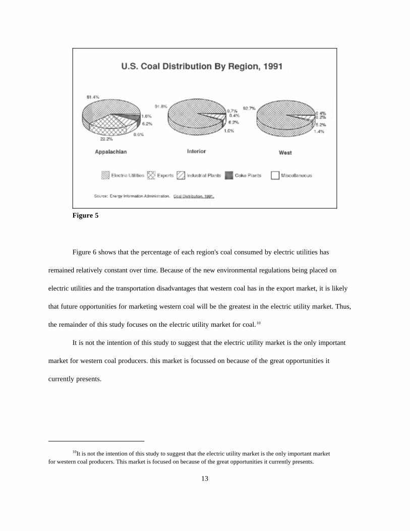
When examining the consumption of the coal produced by the individual regions, it is apparent that

the West and Interior regions market their coal almost exclusively to electric utilities (Figure 5). The

geographic location and transportation options available to Appalachian producers is somewhat

responsible for the increased share of Appalachian coal being exported and consumed by domestic coke

plants. However, some of this increase also is due to coal qualities. Because coking requires very high

heat levels, anthracite is often the preferred coal for this process. Moreover, the concentration of

environmental laws on domestic utilities makes their demand for low sulfur coal the greatest.

10It is not the intention of this study to suggest that the electric utility market is the only important marketfor western coal producers. This market is focused on because of the great opportunities it currently presents.

13

Figure 5

Figure 6 shows that the percentage of each region's coal consumed by electric utilities has

remained relatively constant over time. Because of the new environmental regulations being placed on

electric utilities and the transportation disadvantages that western coal has in the export market, it is likely

that future opportunities for marketing western coal will be the greatest in the electric utility market. Thus,

the remainder of this study focuses on the electric utility market for coal.10

It is not the intention of this study to suggest that the electric utility market is the only important

market for western coal producers. this market is focussed on because of the great opportunities it

currently presents.

14

Figure 6

Electricity Demand Regions

The nine regions defined by the U.S. Bureau of Census, can be used to examine coal demand by

electric utilities in the U.S. (Figure 7). These regions include New England, Middle Atlantic, East North

Central, West North Central, South Atlantic, East South Central, West South Central, Mountain and

Pacific regions.

15

Figure 7

In 1991, five of these regions accounted for more than eighty percent of the coal receipts by

electric utilities nationwide (Figure 8). Moreover, the top three regions received more than half of the coal

received by U.S. electric utilities.

16

Figure 8

Figure 9 shows that the quantity of coal demanded by electric utilities has increased greatly since

1980. In the period between 1980 and 1991, the East North Central region has had the largest demand for

coal by electric utilities. The West South Central region had the sixth highest quantity demanded by

electric utilities in 1980 but its use of coal increased over the time period making it the second largest

demander of coal for electricity generation by 1991. The South Atlantic region was the second largest

consumer of coal for electricity generation throughout most of the period, but consumed slightly less than

the West South Central region in 1991. The other major consumption regions during this time period were

the West North Central region and the Mountain region. The remainder of this section will focus on these

five regions.

17

Figure 9

East North Central Region

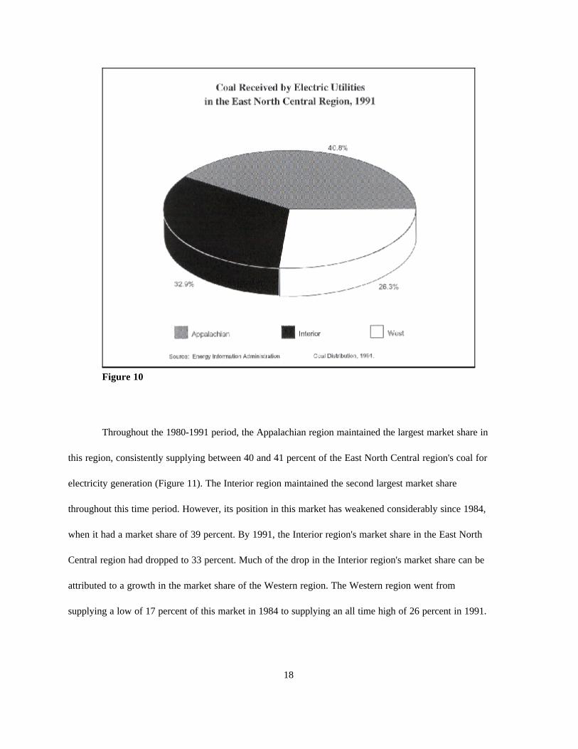
In 1991, the Appalachian region supplied nearly 41 percent of the coal received by electric utilities

in the East North Central region (Figure 10). The Interior region supplied the second most coal to this

region, or about 33 percent. The West region's 26 percent share of this market is remarkable, considering

the proximity of the market to the Appalachian and Interior producing regions.

18

Figure 10

Throughout the 1980-1991 period, the Appalachian region maintained the largest market share in

this region, consistently supplying between 40 and 41 percent of the East North Central region's coal for

electricity generation (Figure 11). The Interior region maintained the second largest market share

throughout this time period. However, its position in this market has weakened considerably since 1984,

when it had a market share of 39 percent. By 1991, the Interior region's market share in the East North

Central region had dropped to 33 percent. Much of the drop in the Interior region's market share can be

attributed to a growth in the market share of the Western region. The Western region went from

supplying a low of 17 percent of this market in 1984 to supplying an all time high of 26 percent in 1991.

19

Figure 11

This penetration by western coal producers at the expense of interior coal producers provides an excellent

example of the growing importance of sulfur content in coal purchases. Despite the fact that

this demand region encompasses much of the coal reserves in the Interior region, the high sulfur content

of this coal has reduced its desirability. Furthermore, entry of the Chicago and Northwestern into the

Powder River Basin in 1984 has increased transportation competitiveness to an area that previously had

only one transportation option.

20

Figure 12

West South Central Region

As Figure 12 shows, the West region supplied more than half the coal used for electricity

generation in the West South Central region in 1991. The Interior region also has a strong market share in

this region, supplying more than 43 percent in 1991. This is not surprising, since the majority of the

demand for coal for electricity generation in this region is in Texas, and the majority of low-sulfur coal

reserves in this region are in Texas (low sulfur lignite). The Appalachian region's 1991 market share in

this region was essentially zero.

21

Figure 13

Figure 13 shows the steady growth in this market between 1980 and 1991 when the West region

was its leading supplier. In 1980, the Western producing region had a market share of 53 percent. After a

growth in market share to a level of 62 percent in 1984, its market share has leveled off somewhat with

the West region supplying 57 percent of the coal used for electricity generation in 1991. The Interior

region supplied the remainder of this market throughout the period.

22

Figure 14

South Atlantic Region

In 1991, the Appalachian producing region dominated the market for coal by electric utilities in the

South Atlantic. It supplied nearly 87 percent of the coal to this market (Figure 14). In contrast, the Interior

region supplied approximately 12 percent of the coal received by electric utilities in this region in 1991.

The West region supplied only 1 percent. The low market share of the West region is apparently the

result of a lack of proximity to this market caused by long distances and a lack of transportation

alternatives resulting in high transportation rates for western coal shipping. In addition, the heart of the

low sulfur Appalachian reserves are in eastern Kentucky, southern West Virginia, and Virginia, in close

proximity to the market.

23

Figure 15

Throughout the 1980-1991 period, the Appalachian producing region dominated this market,

consistently supplying more than 86 percent of the coal received by electric utilities in the South Atlantic

(Figure 15). The Interior region supplied most of the remaining coal demanded throughout this period.

While the West generally supplied 0 percent of the coal demanded by electric utilities in this region

throughout the 1980s, the West gained a market share of 2 and 1 percent in 1990 and 1991, respectively.

Although this is not a significant amount of coal, this market could develop into a significant one for

western producers. The small amounts of coal shipped to this market in 1990 and 1991 suggest that in

some cases the advantages that western coal has over interior coal in sulfur content may be able to

overcome its transportation disadvantage in this market. However, the potential to displace Appalachian

coal in this market appears to be small due to the proximity of low sulfur Appalachian coal to this market.

24

Figure 16

West North Central Region

In 1991, the West producing region dominated the West North Central region's electric utility

market for coal by supplying more than 81 percent of the 77 million tons received (Figure 16). The

Interior region supplied most of the remaining coal received by electric utilities in this region;

approximately eighteen percent. The Appalachian region's market share was less than one percent in

1991 .

25

Figure 17

The West North Central region provides an excellent example of a market where the Western

production region was able to increase its share over time because of an increasing demand for low sulfur

coal and an increase in western transportation competitiveness (Figure 17). In 1980, the Western coal

production region supplied 67 percent of the West North Central market for coal by electric utilities. This

share steadily rose to a high of 81 beginning in 1984. This occurred as the Chicago Northwestern gained

access to the Powder River Basin in Wyoming; an area previously served solely by the Burlington

Northern. By contrast, the Interior production region's market share dropped from 32 to 18 percent

between 1980 and 1991. This is remarkable, as a large concentration of this region's coal receipts have

been in Missouri, Minnesota, and Iowa; states near the heart of the Interior coal reserves.

26

Figure 18

Mountain Region

Virtually all of the coal received by electric utilities in the Mountain region was supplied

by the West producing region in 1991 (Figure 18). This was the case throughout the 1980-1991 period.

This market is an example of the Western producing region's dominance where proximity exists.

When considered collectively, these five electric utility markets consumed more than 630 million

tons of coal in 1991. The Western producing region supplied more than 49 percent of this coal, or

approximately 310 million tons.

11In Figures 19 and 20, the method of transportation is defined as follows: water transportation includescoal hauled to or from water loading facilities by other modes of transportation; rail transportation includes coalhauled to or from the railroad siding by truck; truck transportation includes shipments where truck was used as theonly mode of transportation.

12This pipeline is the Black Mesa Pipeline that travels from Black Mesa, Arizona, to southern Nevada.

27

Coal Transportation

Several transportation options exist for coal producers nationwide. However, the majority

of coal in the United States is transported by rail; approximately 58 percent of the total in 1991 (Figure

19).11 The second leading mode of transportation in the United States for delivering coal in 1991 was

water transportation. Most of the coal delivered by water in the U.S. makes use of the inland river

system, while few transporters use the Great Lakes and tidewater ports. The third leading mode of

transportation for coal in 1991 was tramway, conveyer, and slurry pipeline. Tramway and conveyer

movements generally travel very short distances and are the primary methods of transporting coal to mine

mouth power plants. On the other hand, the only coal slurry pipeline in operation in the U.S. travels a

distance of 273 miles.12 Finally, only 11 percent of the nation's coal moves solely by truck. These

movements generally cover short distances.

28

Figure 19

29

Figure 20

As Figure 20 shows, the West region is far more dependent on rail for transporting its coal than

its eastern counterparts. In 1991, nearly 70 percent of the West regions shipments were transported by

rail, 6 percent were transported by water, and 5 percent were transported by truck. By comparison, the

Appalachian and Interior regions transported 55 and 43 percent of their shipments by rail in 1991,

respectively. Moreover, they transported 23 percent and 26 percent of their coal by water, respectively,

and 14 percent and 17 percent by truck, respectively. The larger percentages of shipments transported by

water and truck from the Appalachian and Interior regions are a function of their proximity to the inland

waterway system, and their proximity to major markets. The larger percentage of West coal shipments

that are transported by tramway, conveyer and slurry pipeline is primarily a function of the sizeable mine

mouth generation in the west.

30

Figure 21

Figure 21 shows that the West region has traditionally been much more dependent on rail for

transporting coal than the Appalachian or Interior regions. The heavy dependence on rail for transporting

coal to consumers by western producers suggests that continued efficient rail transportation is essential to

future marketing opportunities. Because of this dependence on rail, much of the remainder of this study

focuses on rail transportation of coal to electric utilities.

31

Figure 22

Rail Transportation of Western Coal

As Figure 22 shows, coal is an important commodity for the railroads in terms of total freight and

revenues. Coal comprises the most tonnage originated and the highest percentage of revenues of any

commodity hauled by Class I railroads. In 1991, coal represented 41 percent of revenue freight originated

and 23 percent of total revenues for Class I railroads. The second leading commodity in terms of tonnage

originated was farm products, at 10 percent. The second leading commodity in terms of revenues was

non-metallic minerals, representing 13 percent of revenues.

13Fieldston Coal Transportation Manual, 1991.

14Moody’s Transportation Manual is used to obtain 1994 carloadings and revenues when available.

32

In 1980, coal represented only 11 percent of total revenue freight originated, and 25 percent of

revenue earned. Since that time, coal has grown in importance for the railroads and has consistently

represented 35 to 41 percent of freight tonnage originated and 21 to 25 percent of total revenues for Class

I railroads. Much of this increase in importance of coal as a commodity for railroads can be attributed to

the increased exploitation of western coal reserves. The major coal hauling railroads in the west are

discussed briefly in the following paragraphs.

There are eight major coal hauling railroads serving western producers.13 These include the

Atchison, Topeka, and Santa Fe, the Burlington Northern, the Chicago & Northwestern, the Denver &

Rio Grande, the Kansas City Southern, the Southern Pacific, the Union Pacific, and Utah Railway. Seven

of these railroads are Class I railroads, while the Utah is a regional railroad.

The Atchison, Topeka, and Santa Fe (ATSF) serves coal producers in Colfax and McKinley

counties in New Mexico. Furthermore, the ATSF handles coal shipments originated by other carriers in

the Powder River Basin and in Colorado. In 1989, coal represented only 8 percent of the ATSF's freight

revenue, as the railroad carried more than 28 million tons of coal; 8.5 million which were originated by the

ATSF.

The Burlington Northern is the west's largest coal hauling railroad, carrying over 172 million tons

of coal in 1994, and originating more than 166 million tons.14 Coal also represents BN's most important

commodity in terms of freight revenue and accounted for more than 33 percent of revenues in 1994. The

BN originates more than 90 percent of its coal in the Powder River Basin in Wyoming and Montana - an

area that accounts for approximately 60 percent of annual coal production in the west. Other origins of

coal by the BN include coal produced in the Illinois Basin, Oklahoma, and North Dakota.

33

Until 1984, the Burlington Northern essentially had a monopoly in the Powder River Basin. In

1984, Western Rail Properties, Inc. (WRPI), a subsidiary of the Chicago & North Western opened, a

connector line with the Union Pacific that allowed it to transport coal from the southern portion of the

Powder River Basin in Wyoming. In 1986, after the Interstate Commerce Commission (ICC) gave the

C&NW permission to build and operate a 10.7 mile spur north of its existing terminal in the PRB, the BN

agreed to sell half of the interest in its existing line to the C&NW. Since that time coal has become the

C&NW's leading revenue producing commodity, supplying more than 26 percent of freight revenues in

1989, and accounting for more than 65 million tons; 45 million that were originated. Almost all of the

C&NW's coal traffic is originated from the Powder River Basin.

The Union Pacific (UP) serves coal producers in the Illinois Basin and the Hanna Basin in

Wyoming. However, most of the UP's coal traffic originates in the Powder River Basin on WRPI or in

the Uinta Basin in western Colorado and eastern Utah on the Utah Railway and the Denver & Rio

Grande Western. The UP is a major western coal hauler, hauling more than 129 million tons of coal in

1994, and originating more than 20 million tons in 1994. In 1994 coal was the second leading commodity

hauled on the UP in terms of revenue.

The Denver & Rio Grande Western purchased the Southern Pacific railroad and the St. Louis

Southwestern railroad in 1988. These lines operate as one integrated system and are referred to as

Southern Pacific Lines (SPL). These lines serve metallurgical (coking) coal producers and steam coal

producers in Colorado and Utah. In 1989, coal was the SPL's seventh leading commodity accounting for

more than 15 million tons, almost all of which was originated by SPL.

The Kansas City Southern (KCS) railroad hauled more than 15 million tons of coal in 1989,

accounting for more than 32 percent of the KCS's revenues in 1989. The KCS serves mostly as a

terminating carrier of coal traffic. The KCS terminates much of the coal traffic that originates in the

34

Powder River Basin on the Burlington Northern and the Chicago & North Western. KCS also originates

some coal in Texas.

Finally, the Utah railway (UTAH) serves coal producers in Carbon and Emery Counties in Utah.

In 1989, the UTAH originated about four million tons of coal in these counties. This traffic accounted for

more than 99 percent of the carrier's traffic, most of which was interchanged with the UP.

The purpose of this section has been to highlight some the major transporters of western coal, and

to illustrate the importance of coal to these railroads. Later in the report, competition between railroads

will be examined, along with the effects of competition on rates. The next section of the study highlights

the history of environmental regulations, and their effects on coal production and markets.

THE CLEAN AIR ACT AMENDMENTS OF 1990

The Clean Air Act Amendments of 1990 were considered a major breakthrough in the nation's

and the world's fight against environmental decline. The Clean Air Act of 1990 not only expanded and

strengthened existing environmental law, but included a new market-based approach to dealing with the

problem of acid rain. The market-based approach for dealing with the problem of acid rain provides a

pivotal market opportunity for western coal producers. This section of the report reviews some of the

history of environmental laws, how the recent changes represent a marked change in environmental

regulation, and how these changes provide opportunity for western coal interests.

The first major federal environmental policy took place in 1963 with the passage of the Clean Air

Act. This act increased funding for researching the causes of pollution, and established a legal process for

municipalities, states, and the federal government to take regulatory action against sources of pollution.

The act gave some focus to emissions by stationary sources such as electric utilities, but placed the major

focus of pollution control on automobile emissions.

15Bryner, Gary C. Blue Skies, Green Politics - The Clean Air Act of 1990.

16Ibid.

35

In 1967, the first attempt by the federal government to create standards for air pollution was

made with the passage of the Air Quality Act. This Act called for the establishment of metropolitan air

quality regions throughout the United States. Air quality standards were to be developed by states with

plans implemented to achieve them. Failure to establish standards and implement plans by the states could

result in federal government intervention by the Department of Health, Education, and Welfare.

Implementation of the provisions of this act was slow to develop, as the federal government had

designated only a small portion of air quality regions. States had not established standards or implemented

plans by 1970.15 Moreover, this act did not establish specific standards for stationary sources such as

electric utilities.

As a result of the lack of comprehensive regulations and a concern about the comparative

disadvantages that were possible for firms in states where standards and plans were being implemented,

President Richard Nixon called for extensive environmental regulations in his January 1970 State of the

Union address.16 In December of 1970, the Clean Air Act was passed. It shifted the responsibility of

developing air quality standards to the federal government (through national ambient air quality standards),

but continued to place the burden of implementation plans on the states. Thus, while each plan was to

include limitations for pollution emissions from stationary sources (e.g. electric utilities), the limitations

placed on existing electric utilities could vary widely among states based on the implementation plans put

in place by the states. However, some nationwide regulations on new electric utilities regarding emissions

were put in place.

The next major piece of legislation that attempted to reduce nationwide pollution levels was the

Clean Air Act Amendments of 1977. In the face of a shutdown of automobile production due to a failure

17Earlier legislation had mandated that tailpipe emission standards be met by the 1978 model year. Theautomobile industry had indicated that these standards would not be met. Bryner, Gary C. Blue Skies, Green Politics- The Clean Air Act of 1990.

18See Ackerman and Hassler. Clean Coal/Dirty Air - or How the Clean Air Act Became a Multibillion-Dollar Bail-Out for High Sulfur Coal Producers and What Should Be Done About It.

36

to meet tailpipe emission standards, President Jimmy Carter urged Congress to pass amendments before

the August congressional recess.17 The amendments extended the deadlines for meeting various pollution

levels and standards by regions, cities, and industries. However, the amendments also increased penalties

for noncompliance by stationary sources of pollution, and called for state collection of permit fees from

these sources. This act contained a key provision that affected the regional distribution and market share

of coal producers. This provision required that all new fossil-fuel burning utilities install scrubbers. This

stipulation, in essence, prevented high sulfur coal producers in the east from being at a competitive

disadvantage.18 It not only prevented western coal producers from realizing a prime opportunity in terms

of market share and production, but it prevented electric utilities from choosing the least cost method of

reducing emissions of pollutants. Authorization for the Clean Air Act ended in 1981. Funding for the

implementation of this act was achieved by Congress continually passing appropriations resolutions.

Several industry groups, as well as environmental groups, were not satisfied with the 1977

amendments and sought revisions of the Clean Air Act. Industry groups pointed to problems in the Act

such as its failure to take into consideration the costs of pollution control equipment, the high price of

acquiring permits, and other various provisions. Environmentalists and many in congress were dissatisfied

with the perceived lenient methods of enforcement of the Act by the Environmental Protection Agency.

The problem of acid rain also had been linked to the emission of sulfur dioxide (SO,) and nitrogen oxides

(NO), and the requirement to install scrubbers in plants built since 1977 had largely ignored the major

problem of sulfur dioxide emissions, since older plants constituted such a large portion of coal burned.

19Bryner, Gary C. Blue Skies, Green Politics - The Clean Air Act of 1990.

20Bryner, Gary C. Blue Skies, Green Politics - The Clean Air Act of 1990.

37

Steps toward reducing acid rain producing emissions were deemed as important for international relations

(particularly with Canada), and as an important issue to the American public.19

Throughout the 1980s attempts to amend the Clean Air Act were made, but without resolution

due to the conflicting regional, industrial, and environmental interests. Two changes in leadership were

considered major breakthroughs in the efforts to amend the Clean Air Act: the election of George Bush as

president, and the replacement of Robert Byrd as Senate Majority Leader with George Mitchell.20 Bush

had made several campaign promises regarding the environment, and used environmental issues to

distance himself from Ronald Reagan. Byrd had consistently blocked efforts to amend the Clean Air Act,

as he was concerned about the loss of jobs in the coal mining industry in West Virginia where high sulfur

coal is produced. Furthermore, Mitchell had been one of the leaders in the attempts to amend the Clean

Air Act. Both of these developments renewed the belief that effective amendments to the Clean Air Act

could be put in place.

In 1989, the Bush Administration introduced an amended Clean Air Act that was markedly

different from previous environmental law. The bill contained an innovative market approach that dealt

with the problem of acid rain. Whereas traditional environmental regulation placed limitations on pollution

sources in terms of the amounts that they could emit, the Bush bill provided a method for allocating

pollution rights in the most cost-effective manner. In 1990, the Clean Air Act was finally amended by

Congress. In many ways, the act was similar to the bill introduced by the Bush Administration.

For the most part, the Clean Air Act as amended represents a comprehensive, economic, and

longrange plan for pollution control. The major provision of the Act is Title IV, the acid rain provision.

Likewise, this is the provision that is likely to have the greatest effect on coal production and coal markets,

21Energy Information Administration. Annual Outlook for U.S. Electric Power, 1991.

22Federal Register. 40 CFR Parts 72 and 73 - Acid Rain Allowance Allocations and Reserves; ProposedRules.

23Federal Register. 40 CFR Parts 72 and 73 - Acid Rain Allowance Allocations and Reserves; ProposedRules.

38

nationwide. The following paragraphs explain the causes of acid rain and highlight the provisions

associated with reducing it in the 1990 Clean Air Act Amendments.

In 1990, more than 70 percent of all electricity was generated from fossil fuels, and more than 50

percent from coal.21 When fossil fuels are burned, significant amounts of sulfur dioxide (SO2) and

nitrogen oxides (NOx) are emitted. Coal and oil are the two highest emitters of these substances.

Scientific evidence has shown that several chemical reactions can occur to sulfur dioxide and nitrogen

oxides when they are released into the atmosphere causing their transformation into various chemical

products such as sulfates, nitrates, sulfuric acid, and nitric acid.22 Furthermore, these chemical products

can travel several miles or fall to the ground near their source, dropping to the earth in dry form as gases,

aerosols, or particulates, or in wet form as rain, fog, or snow. Damage to the environment and animals has

led many to believe that these forms of pollution also represent a threat to human health.

The 1990 Clean Air Act targets electric utilities for reducing the emissions of SO, and NO,,,

because more than two-thirds of all SO, emissions and more than one-third of NO,, emissions are the

result of the generation of electricity.23 The Act has a goal of reducing total annual sulfur dioxide

emissions by electric utilities to 10 million tons below the level emitted in 1980, calling for a national cap of

8.95 million tons of sulfur dioxide emissions per year by electric utilities. Furthermore, nitrogen oxides also

must be reduced by electric utilities. While both of these acid rain-contributing chemicals are reduced by

the Act, the approach used to reduce each is very dissimilar. The reduction of nitrogen oxides is done with

the traditional approach of mandating the use of a certain technology. The reduction of sulfur dioxide is

24It is important to remember that the Clean Air Act (as amended) does not consider the regionaldistribution of sulfur dioxide. Only the total nationwide production of SO2 is considered. Several observers haveleveled criticism at the amendments for this reason.

25Again, it is important to remember that this ignores the distributional impacts of sulfur emissions on theenvironment.

39

achieved by limiting total nationwide emissions and allowing those utilities whose costs of reducing

emissions are highest to keep on polluting. Thus, the important factor in the amendments that is likely to

affect market shares of various coal producers is the SO2 reduction provision.

The nationwide24 reduction of sulfur dioxide is to be achieved in three stages. The first stage of

the reduction occurred on Jan. 1, 1995, when the 110 largest utilities located in 21 states were required to

collectively meet an intermediate level of SO2 emissions (averaging 2.5 pounds of sulfur dioxide per

million BTU used on average from 1985 through 1987) as a maximum. This stage was officially known as

Phase I. The second stage of the reduction occurs on Jan. 1, 2000, when essentially all electric utilities in

the contiguous United States are required to collectively meet another intermediate (but more stringent)

level of SO2 emissions (averaging 1.2 pounds of sulfur dioxide per million BTU used on average from

1985 through 1987) as a maximum. This stage is known as Phase II, part 1. In the second part of Phase

II and beginning in the year 2010, the same electric utilities must collectively reduce sulfur dioxide

emissions even further.

Achievement of the various reductions discussed above is realized through a nationwide allocation

of sulfur dioxide emission allowances. Each allowance provides the right to emit one ton of sulfur dioxide

and can be used by any electric utility. Thus, electric utilities can freely buy and sell sulfur dioxide

allowances. They are not bound by any other mandate in regard to sulfur dioxide emissions than to have

an allowance for every ton that is emitted. By allowing utilities to trade pollution rights, the most

cost-effective solution to reducing pollution should be achieved in theory.25 This should occur, since

26Energy Information Administration. Estimation of U.S. Coal Reserves by Coal Type - Heat and SulfurContent.

40

utilities that would incur high costs from reducing emissions will place a higher value on the sulfur

allowances than the utilities where the costs from reducing emissions are not so high. Thus, in an open

bidding process, the minimum total costs of pollution control should be achieved as the utilities where the

costs of reducing emissions are high will purchase allowances at a price less than or equal to the cost of

reducing emissions, while the utilities where the costs of reducing emissions are low will reduce emissions

rather than holding allowances.

In many cases the lowest cost method of reducing pollution is likely to be low sulfur coal, as the

costs associated with scrubber installation and maintenance are very high. Since more than 86 percent of

recoverable low sulfur coal reserves (those emitting less than 1.2 pounds of sulfur dioxide per million

British Thermal Units (BTUs) of heat inputs) are located in the west, a great opportunity for market

expansion exists for western coal producers.26 Because of the great distances that western coal

producers are from most major population centers, rail transportation will play a critical role in the ability

of western coal producers to capitalize on this opportunity. The next section of the report examines rail

rates for hauling coal, focussing on the competitive factors influencing rates.

Rail Rates for Coal Transport

As shown previously, nearly two-thirds of western coal is transported by rail to its final

destination. Since most of the electric utilities located at distances from western mines where trucking is

cost competitive already use western coal, it is likely that most of the future growth in western coal

production will depend on low cost rail transportation to shippers. Long distances from consumption

regions increase the portion of delivered coal costs of western coal that is due to transportation, and

41

therefore magnify the importance of efficient transportation for western coal producers. This section of

the report presents a model of rail rates and highlights factors influencing rates that differ between

western, midwestern, and eastern coal shipments.

Several studies have examined coal rail rates and the economic rents captured by railroads in

transporting western coal. Three of these studies are reviewed in the following paragraphs.

Atkinson and Kerkvliet (1986) developed a model to estimate economic rents captured by

railroads, mines, electric utilities, and the state for Wyoming low sulfur coal sold to electric utilities. They

measured maximum potential rent captured by the buyer or the seller as the difference between the price

of a substitute input and the marginal cost of production (including rail transport). Using a 1980-1982 data

set, they found that railroads and coal producers each captured 23 percent of potential rents and that

electric utilities captured 47 percent of potential rents. They found that since railroad deregulation, rents

shifted toward the railroads. Their study also examined the extent of discriminatory pricing by railroads

and coal producers. Their model for examining price discrimination by railroads measures the variation in

the percentage markup of rail rates over marginal costs by the volume of coal purchased — a dummy

variable equal to unity when the best alternative fuel for the utility is another

coal — the percentage contribution of Wyoming coal to BTU input, and the date when the coal contract

was signed. The only significant variables in this estimation were volume and the percentage contribution

of Wyoming coal to BTU input. Volume had a negative sign suggesting that the elasticity of demand for

Wyoming coal was higher for high volume purchasers. The percentage contribution of Wyoming coal to

BTU input had a positive sign suggesting that the elasticity of demand is lower for utilities that are heavily

dependent on Wyoming low sulfur coal.

Garrod and Miklius (1987) also attempted to measure the ability of railroads to capture rents in

the shipment of western coal after deregulation. The authors focused on western coal shipments because

42

of their similarity to a captive market. They estimated the portion of the rents captured by railroads as the

outcome of an indeterminate bargaining process between railroads and electric utilities. Economic rents

were measured in several ways. First, they measured potential economic rents as the difference between

the delivered price of natural gas and the summation of railroad cost and mine mouth price of delivering

western coal. In estimating the economic rent captured by railroads in this way, they found that railroads

captured a smaller share of rents in 1983 than in 1970, but a larger real dollar amount of rents. Next, they

measured potential economic rents as the difference between the delivered price of the best alternative

coal and the summation of the railroad cost and mine mouth price of delivering western coal. When

estimating economic rents captured with this definition, assuming that western railroads take eastern and

midwestern coal rates as a given, they found that railroads serving western coal mines captured almost 20

percent of the potential rent. When estimating, this model assumed that western, eastern, and midwestern

rail rates are determined simultaneously, they found that railroads captured 25 percent of potential rents.

The authors show that if utilities were truly captive, one would expect the railroads' share of monopoly

rent to be one. They suggest that other factors such as geographic competition may constrain railroad

pricing power.

Dunbar and Mehring (1990) use the Public Use Waybill sample to construct a hedonic price index

for rail coal prices between 1973 and 1983. To construct this price index, they regressed real rail

revenues per ton-mile for certain origin-destination pairs on distance and volume. They then fixed volume

and distance at their 1973 levels to estimate 1978 and 1983 rail rates at 1973 volume and distance levels.

This allowed them to examine rail coal rate changes not due to changes in volume and distance. They

found that rail coal rates have increased slightly since deregulation, but that some markets have realized

rate decreases while others have realized increases.

43

Determinants of Variations in Rail Coal Rates

This study does not attempt to measure rents obtained by railroads in shipping coal. A rail rate

model was formulated for purposes of providing a greater understanding of factors influencing rail rate

variations and for providing predicted rail rates between all origins and destinations of coal to be used in a

later section of the report. Rail rates for coal shipments are examined in this study by an analysis of

revenue per ton-mile for electric utility contract shipments of coal. Revenue per ton-mile standardizes rail

rates on a volume and distance basis for comparison.

Almost all coal is purchased under supply contracts that last one year or more. Nearly 75 percent

of the coal supply contracts in existence in 1986 and 1987 were for more than 11 years. Such long-term

contracts are prevalent, as utilities attempt to obtain a stably priced future supply of coal. Because of the

desire to assure a stable price for some future time period, rail contracts to transport the coal typically

coincide with the coal supply contracts. Thus, an analysis of factors influencing rail rates should examine

relevant factors at the time when the coal supply contract (and probably the rail contract) was made. This

study makes use of a data set that provides information on when coal supply contracts were made.

To examine the variation in rail rates per ton-mile for annual rail volumes of coal moving between

coal mines and electric utilities, the influence of supply characteristics and factors influencing the price

elasticity of demand are considered. The general model used to explain rail rates for coal is as follows:

R = R(S,D)

where: R = revenue per ton-mileS = a vector of supply characteristicsD = a vector of variables affecting the elasticity of demand.

44

The vector of supply characteristics includes factors influencing costs such as shipment distance,

annual volume shipped, and shipment size. These variables all are expected to have a negative influence

on revenue per ton-mile, as each displays a negative relationship with unit costs. The vector of supply

characteristics also includes the number of railroads in the origin county, as a proxy for market

concentration and is expected to have a negative influence on rates.

The vector of variables influencing the elasticity of demand for rail service includes the distance

of the origin county from coal barge loading facilities, the prices of alternative fuels at the destination in

the year that the coal supply contract was negotiated, and regional and product dummy variables. The

distance of the origin county from barge loading facilities and the prices of alternative fuels at the

destination are expected to have a positive influence on rates, while the product and regional dummy

variables have indeterminant signs, a priori. The specific model used to estimate coal rail rates is the

following:

InRTM = $0 + $1lnVOL + $2lnDIST + $3lnUNIT + $4lnNRR +

$5InBDIST + $6lnALTF + $70WNRC + Quality Dummies +

Regional Dummies

where: RTM = revenue per ton-mileVOL = annual volume shipped over a given routeDIST = rail distance between the origin and destinationUNIT = dummy variable for unit train shipments (1 =unit, 0=single/multi)NRR = number of railroads in the origin countyBDIST = distance of the origin from the nearest coal barge loading facilityALTF = alternative fuel price at the destination in the first year of the coal

contract (average of oil and natural gas price at the destination)OWNRC = dummy variable for private ownership of rail cars.

The log-linear specification used allows the estimation of non-linear relationships with a model

that does not violate the classical assumption of linearity in parameters. The specification allows the

parameter estimates to be interpreted as elasticities.

45

Each of these variables is expected to have an important relationship with rail rates for coal.

Because the model does not include a measure of individual shipment size other than the unit train dummy

variable, annual shipment volume measures two effects: the effect of individual shipment size on rates,

and the effect of annual volume on rates. Both of these effects are expected to be negative. First, many

rail costs such as clerical costs, train crew wages, and locomotive ownership costs are relatively fixed

with respect to the volume of an individual shipment. Thus, as individual shipment volume increases, unit

costs per ton decline at a decreasing rate. Because variables affecting the elasticity of demand for rail

service and the supply characteristics of the rail service are included in the regression, the volume

variable is expected to have a negative sign. Second, large volume shippers are likely to have greater

bargaining power with the railroads in negotiating shipments, and thus, are likely to experience lower

rates, all else constant.

Shipment distance also is expected to have a negative influence on rail rates for coal. Many rail

costs such as loading and unloading costs and clerical costs are incurred for every rail movement, and are

invariant to distance. These costs are referred to as terminal costs. As rail distance increases, these

terminal costs become a smaller portion of total shipment costs that cause costs per mile to decrease.

Revenues per ton-mile also are expected to decrease with distance, since demand and other cost

variables are included.

In the data sample used, there are single car and unit train shipments. Unit train shipments are

those train shipments that are made as part of a dedicated service between a particular origin and

destination. They generally are comprised of very large shipment sizes. Because of the increased

efficiency associated with such a dedicated service and with large car size blocks, and because other

relevant demand and supply factors are included in the estimation, the parameter estimate of the unit train

dummy is expected to be negative.

46

The number of railroads in the origin county is included as a proxy for the degree of intramodal

competition realized for a given movement. As the number of carriers in the origin county is increased,

the potential for different railroads to compete in direct movements or in interconnections with other

railroads increases. Thus, the number of railroads in the origin county is expected to have a negative

influence on the revenue per ton-mile realized.

In measuring the degree of intermodal competition, competition is considered for long-haul

shipments only. For short-haul movements, the only mode that is cost competitive with rail, and is often

preferred to rail, is trucking. Because of the vast interstate highway system in the U.S. and the lack of

barriers to entry into the trucking industry, the degree of price competition provided by trucks for

short-haul shipments is fairly homogeneous among markets. On long-haul shipments, trucks are not cost

competitive with rail and the only form of transportation that can compete with rail on these shipments is

barge, truck/barge, or rail/barge combinations. Thus, the degree of intermodal competition realized for a

rail coal movement can be proxied by the highway distance of the origin county from coal barge loading

facilities. As this distance increases, the revenue per ton-mile realized for a shipment is expected to

increase, holding all other variables constant.

The dummy variable included for private ownership of cars is expected to have a negative

influence on rail revenue per ton-mile. With private car ownership, the shipper rather than the railroad

incurs the car ownership costs. Thus, rail rates using shipper-owned cars do not include the car rental

charges associated with shipments made with railroad-owned cars.

The natural gas price at the destination and the oil price at the destination, in the year that the coal

supply contract was negotiated, are measures of product competition. Product competition is defined as a

constraint on a rail carrier's market power that results from the receiver's ability to substitute other

commodities for the commodity being shipped, where the substitute commodities are transported by a

47

different carrier. In this case, natural gas price and oil price changes, relative to coal prices at the

destination, may alter the electric utility's fuel choice. The carrier's pricing power should be limited by

these alternative fuel prices, which are expected to have a positive influence on revenue per ton-mile.

Regional and quality dummies also are included to capture the effects of geographic and product

competition. Geographic competition is defined as a limit on rail rates resulting from the receiver's ability

to purchase the same kind of fuel from a different source, when the other source is served by a different

carrier. Quality dummies are expected to measure the effects of both geographic and product

competition. Because there is a wide variation in coal quality in U.S. coal mines and because many

electric utility plants were built for specific types of coal, shipments of coal that are in abundance in

several different regions or are easily substituted for are likely to realize lower rates than those that are

produced in only a few areas and that are not easily substituted for with another coal. Moreover, regional

dummies also are expected to measure geographic and product competition. Shipments of coal from

regions where the primary type of coal produced is also produced abundantly elsewhere, or can easily be

substituted for, are likely to realize lower rates that those from regions where the primary type of coal

produced is not produced abundantly elsewhere and cannot be easily substituted for by another coal. The

next section of the report discusses the data problems in examining rail coal rates and the data base used.

Data

An examination of rail rates for coal presents unique data problems. While the Waybill Sample is

most often used in rail rate analyses, the extensive use of contracts in the rail transport of coal make any

waybill analysis of coal rates misleading. The use of contracts in the rail transport of coal has been

increasing over time, and by 1989 more than 90 percent of all rail coal traffic moved by contract. Often

27See Wolfe for a discussion of the problems associated with using Waybill revenues to approximate actualrevenues.

28The Coal Transportation Rate Data Base (CTRDB) was developed by the Energy InformationAdministration from FERC Form 580.

29Shipments that traveled by more than one mode are not used in the rate analysis, as transportation ratesfor each mode are often not separable.

48

the revenues reported to the ICC on particular movements in the Waybill Sample differ substantially from

actual revenues. 27

This study uses the actual rail revenues reported by utilities in their reports to the Federal Energy

Regulatory Commission (FERC).28 The FERC sample covers all jurisdictional utilities with a steam

electric generating station greater than 50 megawatts. Between 1979 and 1987 these utilities purchased

between 69 and 75 percent of all utility contract tonnage of coal purchased in those years. Due to missing

transportation rates for some records, the coverage of the data used in this estimation is somewhat

smaller.

The rail rate estimation described above is performed using 1991 FERC data for all shipments

that originated and terminated by rail that did not have missing values for transportation rates.29 The next

section of the report shows the rail rate estimation results.

Estimation Results

Table 5 shows the parameter estimates obtained from the rail rate estimation. As the table shows,

the model explains nearly 75 percent of the variation in rail contract rates. All parameter estimates have

the expected signs, and many are significant at conventional levels.

As the table shows, variables affecting the costs of rail shipments all have the expected signs.

Annual volume, the unit train dummy, and distance have parameter estimates that are negative and

significant at the 5 percent level. This suggests that rates per ton-mile decrease at a decreasing rate with

49

increases in annual volume, shipment volume, and distance. The sign on the parameter estimate for the

shipper-owned car's dummy is negative as expected, but is not significant at conventional levels.

TABLE 5: ESTIMATION OF REVENUE PER TON MILE FOR COAL RAIL SHIPMENTS

VARIABLEPARAMETERESTIMATE T-RATIO

Intercept0.2488 0.85

VOL-0.0458 4.06*

DIST-0.5809 18.47*

NRR-0.0604 1.41

BDIST0.0514 2.50*

UNIT-0.1387 2.33*

ALTF0.0865 1.15

OWNRC-0.1613 1.28

Interior Region Dummy-0.3068 3.61*

West Region Dummy-0.0287 0.11

Quality Dummy (sulfur<.41 lbs. permmBTU, mmBTU per Ton 14.98-19.99)

-0.26 0.81

Quality Dummy (sulfur .41-.61bs per -mmBTU, mn1BTU per Ton >26)

0.6145 2.78*

Quality Dummy (sulfur .41-.61bs permmBTU, mmBTU per Ton 23-25.99)

0.2674 0.84

Qualtiy Dummy (sulfur .41-.61bs permmBTU, mmBTU per Ton 14.98-19.99)

-0.3186 0.94

Quality Dummy (sulfur .61-.831bs permmBTU, mmBTU per Ton >26)

0.1532 0.65

TABLE 5: ESTIMATION OF REVENUE PER TON MILE FOR COAL RAIL SHIPMENTS

VARIABLEPARAMETERESTIMATE T-RATIO

50

Quality Dummy (sulfur .61-.831bs permmBTU, mmBTU per Ton 23-25.99)

0.1569 0.95

Quality Dummy (sulfur .61-.83 lbs permmBTU, mmBTU per Ton 14.98-19.99)

-0.625 1.75**

Quality Dummy (sulfur .84-1.67 lbs permmBTU, mmBTU per Ton >26)

0.3421 2.33*

Quality Dummy (sulfur .84-1.671bs permmBTU, mmBTU per Ton 23-25.99)

0.0477 0.33

Quality Dummy (sulfur .84-1.671bs permmBTU, mmBTU per Ton 20-22.99)

0.1304 0.48

Quality Dummy (sulfur .84-1.671bs permmBTU, mmBTU per Ton < 14.98)

-0.2823 0.73

Quality Dummy (sulfur 1.68-2.501bs permmBTU, mmBTU per Ton > 26)

0.4454 3.05*

Quality Dummy (sulfur 1.68-2.501bs permmBTU, mmBTU per Ton 23-25.99)

0.262 1.97*

Quality Dummy (sulfur 1.68-2.501bs permmBTU, mmBTU per Ton 20-22.99)

0.2123 1.29

Quality Dummy (sulfur >2.501bs permmBTU, mmBTU per Ton > 26)

0.6886 3.61*

Quality Dummy (sulfur >2.501bs permmBTU, mmBTU per Ton 23-25.99)

-0.0358 0.32

all continuous variables are in natural logarithms*significant at the 5 percent level**significant at the 10 percent levelAdj. RZ = .7482N=212 F=26.08

The variables used to measure the degree of intermodal and intermodal competition realized for

the rail coal shipments also have the expected signs. The number of railroads, a proxy for the level of

51

intermodal competition, has a negative sign in the estimation suggesting that rail rates decrease with

decreases in railroad market concentration. However, the parameter estimate was not significant at the 5

percent level. The distance from barge loading facilities, a proxy for intermodal competition realized, has a

positive sign and is significant at the 5 percent level. This suggests that barges and truck1barge

combinations effectively serve as rate constraints on rail movements.

Geographic and product competition also appear to play an important role in explaining variations

in rail rates. As Table 5 shows, the sign on the parameter estimate of the average price of alternative

fuels at the destination when the rail contract began is positive, as expected. This suggests, that rail rates

are limited by the electric utility's ability to substitute alternative fuels for coal. While the parameter

estimate is not significant, its t-ratio is above one suggesting an important role for this variable. Many

regional and quality variables are significant as well, and suggest that railroads consider the utility's ability

to obtain fuels from other regions or to substitute other fuels for coal.

This section of the report has shown the important roles that factors influencing the supply and

price elasticity of demand for rail service play in determining rail coal rates. The next section of the report

presents linear programming models that attempt to show the changes in coal flows likely to result from

the Clean Air Act Amendments of 1990.

The Impact of the Clean Air Act Amendments on Western Coal

As mentioned in a previous section of the report, the preponderance of the reduction in sulfur

dioxide emissions by electric utilities is scheduled to occur in the year 2000, when total sulfur dioxide

emissions by electric utilities are limited to 8.95 million tons. While electric utilities are already starting to

plan for the change, a greater knowledge of the change in coal flows will be useful to government

agencies and coal producers.

52

This study simulates coal flows that would take place with a minimization of acquisition costs, and

the impact that the sulfur limitations and potential transportation rate changes are likely to have on coal

flows. This study estimates several linear programming models that provide insight into changes taking

place with the CAAA90 and with potential changes in future transportation rates. The base case linear

program, which provides a starting point for comparing all other linear programs, minimizes total coal

acquisition costs (including transport costs) for electric utilities. Because all of the models make

simplifications and abstractions from reality for purposes of tractability, they will not necessarily

approximate actual coal flows. Thus, it is the comparison of the impact models to the base case that will

provide insight into the possible magnitude of change - not the flows estimated by the various models. The

first impact case model simulates coal flows resulting from a minimization of total coal acquisition and

boiler retrofitting costs for low sulfur coal, subject to the constraint that utilities limit emissions to the 8.95

million tons of sulfur dioxide specified by the CAAA90 (while accounting for the scrubber installations

that are scheduled to take place in Phase I of the CAAA90 as specified in applications to the EPA for

Phase I bonuses). The model is expected to show the maximum amount of switching to low sulfur coal

that could occur due to the CAAA90, with current transportation rates. There are two reasons that the

magnitude of the switch are likely to be overstated. First, some of the coal purchases that currently take

place already include sulfur considerations due to early switching or previous environmental regulations.

Thus, the base case probably understates the portion of total coal purchased by utilities that is low in

sulfur. Second, the impact model does not allow scrubber installation by utilities that do not already have

scrubbers in place. Another impact model estimates the costs of scrubber installation and acquisition costs

under the scenario where utilities must meet the 8.95 million tons of sulfur dioxide limitation by installing

scrubbers. This case estimates the costs of compliance for electric utilities if scrubber installation were

the only option that can be compared to the costs of compliance for electric utilities if switching to low

53

sulfur coal were the only option. It will provide an estimate of where scrubbers could be installed most

efficiently. The other impact models simulate coal flows under a scenario where coal acquisition

(including transportation) costs and boiler retrofitting costs for low sulfur coal are minimized, subject to

CAAA90 sulfur limitations, under various changes in nationwide rail rates. Several recent changes in the

rail industry and its regulation raise the possibility of large future rail rate changes. Due to large

differences among producing regions in the portion of total acquisition costs that are attributed to

transportation, nationwide changes in rail rates could have a significant impact in regional shares of coal

production. These impact models are designed to show the possible magnitude of such changes.

The base case model, which will provide a starting point for assessing the impacts of changes in

the other models, is shown below:

where: Qij = quantity shipped from mines in county I to plants in county j in tonsOpi = average origin price per ton of coal from mines in county Irij = the average rail rate per ton of transporting coal from origin county I to

destination county jBTTi = average BTU per ton of coal from mines in county Iai = capacity in tons of mines in county Ibj = quantity demanded by utilities in county j in BTUs.

In this base case model, there are no constraints on coal sulfur content. The reason that no sulfur

constraints are included in the base case is because previous “clean air” legislation mandated scrubber

installation, rather than allowing utilities to pursue the least cost methods of sulfur reduction. Thus, under

pre-CAAA90 laws, utilities did not have the option of choosing low sulfur coal or scrubber installation

depending on costs. Instead, they installed scrubbers when mandated to do so, and purchased the coal that

54

could provide the most energy production at the least private cost (where transportation is one component

of this cost).

In issuing permits to utilities to emit sulfur dioxide, and allowing these permits to be freely

exchanged, the CAAA90 allow electrical utilities to choose the least cost method of reducing pollution.

They also suggest that a minimization of overall electric utility sulfur dioxide control costs will take place.

The reason is very simple, as shown by a hypothetical example. Suppose that there are a total of two

electrical utilities in the U.S. Utility A has a cost of reducing sulfur dioxide of $300 per ton, while utility B

has a cost of reducing sulfur dioxide of $100 per ton. Further, suppose that each utility has one permit to

emit a ton of sulfur dioxide, and that each utility would emit two tons of sulfur dioxide without any

attempts at reducing pollution. Utility A would be willing to pay a price only slightly smaller than $300 for

utility B's permit, while utility B would be willing to sell its permit for a price slightly higher than $100.

After the sale, utility A will own both permits and utility B will pursue operations aimed at reducing sulfur

dioxide. The total resource cost associated with reducing sulfur dioxide will amount to $200. On the other

hand, under a system where no exchange is allowed, the total resource cost associated with reducing

sulfur dioxide would amount to $400. Thus, under a system where exchange is allowed, mutually

beneficial exchange ensures that firms with the lowest costs of reducing pollution are the ones that use

resources for pollution control.

For each firm that does use resources for pollution control, the lowest cost method of reducing

pollution may entail a switch to low sulfur coal or the installation of a scrubber. The switch to low sulfur

coal may result in higher acquisition costs due to longer distance transportation, or may result in some

capital investment costs, as plants often must be retrofitted to use western coal. Similarly, the installation

of a scrubber will result in capital investment costs. Ideally, an impact case linear (or nonlinear) program

55

would minimize the total scrubbing and acquisition costs of coal, allowing each utility to pursue the least

cost method of reducing pollution. Such a program could be formulated as follows (non-linear program):

56

where: TSE = (Si * 2) (1 - Vj * .9)Qij = quantity shipped from mines in county i to plants in county j in tonsVi = proportion of county j's generation that is scrubbed (Each utility is

assumed to have a scrubber if the plant was built after 1977. Plants thatstated their intention to retrofit for scrubbers to comply with Phase Irequirements also are assumed to have a scrubber.)

SAj = sulfur allowances for utility plants in county j (one allowance permits theplant to emit one ton of sulfur per year)

Opi = average origin price per ton of coal from mines in county iSi = average tons of sulfur per ton of coal from mines in county iERj = the average cost per BTU of retrofitting plants in county j for low sulfur

eastern coal (less than .61 lbs. of sulfur per million BTU)Wrj = the average cost per BTU of retrofitting plants in county j for low sulfur

western coal (less than.61 lbs. of sulfur per million BTU)NSj = new scrubber capacity installed in county jSCj = average cost per BTU of retrofitting and operating scrubbers on plants in

county jBTTi = average BTUs per ton of coal from county iEi = dummy for counties located in the eastern coal producing regionWi = dummy for counties located in the western coal producing regionLSi = dummy for counties where the average sulfur content of coal is less than

.61 lbs. per million BTUPHSi = dummy for destination counties that use coal with a sulfur content of

more than .61bs. per BTU in the base caserij = the average rail rate per ton of transporting coal from origin county i to

destination county jai = capacity in tons of mines in county ibj = quantity demanded by utilities in county in BTUs.

By minimizing the total scrubbing and acquisition cost of coal, and by limiting the total sulfur

dioxide emissions by electrical utilities to the number of allowances issued, the above impact case

nonlinear program would simulate the coal purchases and scrubber installations under circumstances

where the firms with the lowest pollution control costs are those that use resources to control sulfur

dioxide emissions and where each firm uses the lowest cost method of reducing pollution. Thus, the coal

purchases and scrubber installations that are likely to take place under the CAAA90 are simulated by this

model. However, because of the large computer resources needed to estimate this model, it could not be

30The computer program necessary to estimate this model has been written, and the data necessary toestimate it has been collected. However, upon trying to run the model, the computer ran out of memory.

57

estimated in this study.30 Thus, two models are estimated to show the potential extremes of the impacts of

the CAAA90. The first model minimizes acquisition costs and retrofit costs for low sulfur coal subject to

the total sulfur constraint imposed by Phase 11 of the CAAA90, without allowing scrubber installation.

The second model minimizes retrofit and operation costs of new scrubbers installed to meet Phase II

requirements of the CAAA90, without allowing fuel switching.

The first impact case linear program is exactly the same as the linear program that allows utilities

to choose the least cost method of reducing pollution, with the exception of its failure to allow scrubber

installations. As previously stated, the model is likely to overstate the switch to low sulfur coal.

Nonetheless, it will provide insight into the potential magnitude of the switch. The linear program used to

model the first impact case is shown as follows:

where: TSE (Si * 2) (1 - Vj*.9)

Qij quantity shipped from mines in county i to plants in county j in tons

Vj proportion of county j's generation that is scrubbed (Each utility is assumed to have ascrubber if the plant was built after 1977. Plants that stated their intention to retrofitfor scrubbers to comply with Phase I requirements also are assumed to have ascrubber.)

58

SAj sulfur allowances for utility plants in county j (one allowance permits the plant toemit one ton of sulfur per year)

Opi average origin price per ton of coal from mines in county i

Si average tons of sulfur per ton of coal from mines in county iERj the average cost per BTU of retrofitting plants in county j for low sulfur eastern coal

(less than .61 lbs. of sulfur per million BTU)

WRj the average cost per BTU of retrofitting plants in county j for low sulfur westerncoal (less than.61 lbs. of sulfur per million BTU)

BTTi average BTUs per ton of coal from county i

Ei dummy for counties located in the eastern coal producing regionWi dummy for counties located in the western coal producing region

LSi dummy for counties where the average sulfur content of coal is less than .61 lbs. permillion BTU

PHSj dummy for destination counties that use coal with a sulfur content of more than .6lbs. per BTU in the base case

rij the average rail rate per ton of transporting coal from origin county i to destinationcounty j

ai capacity in tons of mines in county i

bj quantity demanded by utilities in county j in BTUs.

While the first impact model overstates the potential coal switching that would take place under

the Phase II requirements of the CAAA90, the second impact model simulates scrubber installations in

the event that CAAA90 sulfur limitations were met without fuel switching. Although neither of the two

models will simulate the coal flow changes that will take place with the Clean Air Act Amendments, each

will provide insight into the potential costs to utilities from switching and from scrubber installation, the

potential extremes in terms of the number of utilities switching or installing scrubbers, and the potential

extremes in terms of the market share gains made by producing regions. Since the first model requires

utilities to meet sulfur limitations through switching and the second requires them to meet sulfur limitations

through scrubber retrofitting, a comparison of utility locations that take the action of switching in impact

Case I to those locations that take the action of installing scrubbers in impact Case II may provide insight

59

into some of the utility locations where there is a definite advantage associated with pursuing one strategy

or the other. The second impact model is formulated as follows:

60

where: Vj = proportion of county j's generation that is scrubbed (Each utility isassumed to have a scrubber if the plant was built after 1977. Plants thatstated their intention to retrofit for scrubbers to comply with Phase Irequirements are also assumed to have a scrubber.)

NSj = new scrubber capacity installed in county jSCj = average cost per BTU of retrofitting and operating scrubbers on plants in county jbj = quantity demanded by utilities in county j in BTUsSAj = sulfur allowances for utility plants in county j (one allowance permits the plant to

emit one ton of sulfur per year)Si = average tons of sulfur per ton of coal from mines in county IQBij = quantity shipped from origin county i to destination county j in the base case

In addition to the two impact case studies presented above, the change in coal flows is simulated

under the model where all sulfur dioxide reductions are made through fuel switching and where

nationwide coal rail rates change. Because of continual improvements in rail productivity, recent changes

in rail regulatory oversight, and a changing structure of the rail industry, it is highly likely that overall real

rail rates will change in the future. By understanding the potential changes in coal flows resulting from

various rail rate changes, a greater understanding of potential market opportunities can be obtained by

making an assessment of the likely future changes in rail rates.

Data Used for the Linear Programs

To estimate these models, several data items are necessary. These include: the origin price of

coal per BTU at each origin mine in the U.S., an estimate of plant retrofitting costs for switching to

61

western coal for those not previously using western coal, identification of plants already using western

coal, an estimate of the rail rate per BTU of transporting coal from each mine to each utility plant, an

estimate of the truck rate per BTU of transporting coal from each mine to each utility plant, an estimate

of the cost of installing and operating scrubbers in utilities not previously equipped with them, an estimate

of sulfur and BTU content of coal produced at each mine, the total number of sulfur allowances available

to all utilities, a three year average of the amount of electricity that has been generated by each utility, the

heat rate - or number of BTUs needed to generate a kilowatt-hour for each utility, and an estimate of the

available reserves of each mine. Descriptions of the data items are provided in Table 6.

Table 6: Data Sources for the Linear Programs

Data Item Source

Average tons of sulfur per ton of coal from eachproducing county

U.S. Geological Survey. Coal Quality Database:Version 1.3.

Average BTU per ton of coal from each producingcounty

U.S. Geological Survey. Coal Quality Database:Version 1.3.

Average price per ton of coal from each producingcounty (1991 $)

Energy Information Administration. ResourceAllocation and Mine Costing Model (1992).

Capacity of mines in each producing county (existingand new)

Energy Information Administration. ResourceAllocation and Mine Costing Model (1992).

Number of railroads in each producing county TRANSCAD - GIS Software and the FRA GIS railroaddatabase

Distance of each producing county to coal bargeloading facilities

TRANSCAD - GIS Software, Oak Ridge Laboratoriesfacilities highway database, and Fieldstone CoalTransportation Manual

Average annual (three year avg. 1991-93) electricutility generation in KWH for each county (totalcounty generation done where coal is the primaryfuel)

Energy Information Administration, EIA 759, “MonthlyPower Plant Report.”

Average heat rate - BTU per KWH - for eachdestination county

Energy Information Administration, EIA 860, “AnnualElectric Generator Report.”

Table 6: Data Sources for the Linear Programs

Data Item Source

62

Average cost per KWH of retrofitting utility plants forlow sulfur eastern and western coal

Case study estimates by Rupinskas and Hiller,“Considerations for Switching from High-Sulfur Coal toLow Sulfur Coal,” are used for estimates of retrofit costsper kilowatt of nameplate capacity. Annualized costs areestimated using a 30 year plant life and an interest rateof 7 percent (annualization factor = .0806).

Year of initial operation for each coal burning utilityplant in the U.S.

Energy Information Administration. Inventory of PowerPlants in the United States, 1993.

Average rail rate from each origin county to eachdestination county

Rail rates are estimated using the rate function shownpreviously, along with the rail distances between eachorigin and destination estimated with TRANSCAD andthe FRA's rail line database, the number of railroads ineach producing county, the distance of each origincounty to barge loading facilities, and mean values ofother variables included in the rate function.

Total Phase II allowances available to utilities thatcurrently use coal to produce electricity

Environmental Protection Agency. Acid RainAllowance Allocations and Reserves; Proposed Rules,and EIA form 759.

Plants that have or will install scrubbers as part ofPhase I requirements

Energy Information Administration. Electric UtilityPhase I Acid Compliance Strategies for the Clean AirAct Amendments of 1990.

Average operating and maintenance costs forretrofitted scrubbers

A study by Decision Analysis Corporation of Virginia,"Regression Models for Analysis of Retrofit Flue GasDesulfurization Unit Cost and Performance," is used toestimate costs per killowatt of nameplate capacity. Thecosts are annualized using the 30 year plant life and 7percent interest used earlier. Annualized costs aredivided by generation to get costs per KWH.

Average retrofit costs for scrubbers Estimated in an ensuing regression.

One important data issue that has not been addressed deals with estimating a scrubber retrofit

cost per killowatt-hour for all electric utilities that don't already have scrubbers in place. Fortunately,

previous estimates of scrubber retrofitting costs have been made.

Two different approaches have been used to estimate the costs associated with scrubber

retrofitting. These two approaches include an econometric approach that uses actual scrubber retrofitting

31Decision Analysis Corporation of Virginia, “Regression Models for Analyzing Retrofit Flue GasDesulfurization Unit Costs and Performance,” report prepared for the Energy Information Administration (Vienna,VA, May 1993).

63

and operation data, and an economic engineering approach that examines the typical characteristics of an

electric boiler and estimates installation costs of the most efficient scrubber retrofit configuration.

There are advantages and disadvantages associated with each approach. Advantages of the

econometric approach are that it uses actual data and shows the variations in costs associated with

different configurations and boiler characteristics. Disadvantages are that it uses data that is based on the

technology in existence at the time of scrubber retrofitting, while the engineering approach makes retrofit

cost estimates based on current technology. Because of the wide variation in the sizes of electrical utility

plants in the U.S., an estimate of retrofitting costs that shows variations with plant size is imperative.

Thus, the econometric approach to estimating scrubber retrofit costs is used.

A previous study by Decision Analysis Corporation (DAC) has estimated both capital

construction costs and operating and maintenance costs for retrofitting electrical utilities with scrubbers

using a sample of 32 utilities that had scrubbers retrofitted to their plants between 1972 and 1990.31 This

sample of 32 included all of the retrofits that occurred on electrical utility plants with at least 100

megawatts of generating capacity that were in operation between 1985 and 1991.

In estimating the capital construction costs, DAC used measures of the retrofit scrubber size

needed for the particular plant, the design operating efficiency of the scrubber, the type of scrubber

technology used, and the vintage of the boiler as explanatory variables. Specifically, their estimation of

capital construction costs was formulated as follows:

CAPKW = $0 + $1FGDMOD + $2MAXMW + $3BGYEAR +

$4SULFDEF + $5TYPE2 + ,

64

where: CAPKW = real installed capital construction costs per killowatt of nameplateelectric capacity

FGDMOD = number of absorber modulesMAXMW = generator nameplate capacity in megawattsBGYEAR = boiler in-service year

SULFDEF = percentage design sulfur removal efficiencyTYPE2 = absorber type dummy variable (1=tray type, 0=otherwise), = error term.

While DAC obtained the expected results in estimating this model, the extremely limited degrees

of freedom provided by the data set and the linear estimation procedure are problematic. While the

sample size of utilities in operation between 1985 and 1991 that had scrubbers retrofitted cannot be

changed, the functional form that was estimated can be.

There is intuitive and empirical support for believing that estimated relationship is not linear. First,

the intuitive support for a nonlinear relationship is provided by examining the reasons for particular sign

expectations on some of the variables. In particular, DAC hypothesized that increases in the size of the

scrubber to be installed would result in decreased capital construction costs per kilowatt of generating

capacity. These economies are presumably the result of a large fixed cost component associated with

retrofitting a scrubber, and some incremental costs associated with increasing scrubber size. Thus, as

scrubber size increases, the fixed cost component becomes a smaller and smaller portion of total costs,

suggesting that average cost decreases. However, this explanation does not suggest that there is a linear

relationship between scrubber size and capital construction costs per kilowatt of generating capacity. It

does suggest that total capital construction costs increase at a decreasing rate with increased scrubber

size and, that as a result, average costs decrease at a decreasing rate with increases in scrubber size.

Similarly, the relationships between average capital construction costs per kilowatt of generating capacity

and the sulfur removal efficiency or the initial year of operation also are unlikely to be linear. In addition to

the intuitive support for nonlinearity, there is empirical support. In using the parameter estimates obtained

65

from the linear model with mean characteristics of all variables except MAXMW, estimated capital

construction costs per kilowatt of generating capacity are negative for some nameplate capacities used in

the sample. This suggests that the linear estimation does not provide a good fit.

Because of the problem, we re-estimated the same model with a semi-log specification. This

allows the nonlinear relationships to be captured with a model that remains linear in parameters.

Specifically, the following specification is used:

CAPKW = $0 + $1FGDMOD + $2MAXMW + $3BGYEAR +

$4SULFDEF + $5TYPE2 + ,

This specification is exactly the same as that used by DAC with the exception of the nonlinear

relationships between the dependent and independent variables. The estimated model is shown in Table 7.

As the table shows, the nonlinear model provides a good fit with an adjusted R2 of .81. The estimated

parameters, along with the mean values of FGDMOD, SULFDEF, and B GYEAR are used to estimate a

scrubber retrofit cost for all electrical utilities that were built before 1977.

Variable

Table 7: Estimation of ln(CAPKW)

Parameter Estimate t-ratioIntercept -0.7123 0.71

FGDMOD 0.3825 4.09*

MAXMW -0.0018 2.43*

BGYEAR 0.0169 1.28

SULFDEFF 0.0486 7.59*

TYPE2 0.4227 1.67

66

*significant at the 5 percent levelAdjusted R2=.8069F = 21.06S.E.E. = 0.4215

Model and Data Issues

As previously discussed, the models used in this study make abstractions from reality so that they

may be tractable. Some important abstractions include, but are not limited to, the model's use of an

exogenous price, the use of only coal burning utilities, and a focus that is strictly on the electrical utility

sector. Certainly, it must be recognized that these and other abstractions also may cause the model results

to stray from reality. However, such abstractions must be made to assure a model that is manageable and

estimable with available resources.

Similarly, the data contains several apparent anomalies. These include apparent inaccuracies in

several prices and coal quality. However, the data used is believed to be the best available. It would be

unscientific to make corrections in apparent anomalies where one is familiar with the data, while not

knowing whether the other data is correct or not. Therefore, this study uses the unaltered data.

Base Model Results

Table 8 shows the coal production simulated by the model that minimizes acquisition costs with no

consideration of sulfur dioxide limitations. As the table shows, western Kentucky is simulated to be the

largest coal producer with a market share of more than 21 percent. Second is Wyoming at nearly 19

percent. If the state tonnages are aggregated into the three producing regions, the base model shows 51

percent of the coal to be produced in the Interior region, 26 percent in the Western region, and 23 percent

in the Appalachian region. This is much different than the actual percentages where approximately 20

percent is produced in the Interior region, 35 percent produced in the Western Region, and 45 percent

67

produced in the Appalachian region. While there are several potential reasons for this, it backs the notion

that the base model is most useful for comparison purposes. These percentages may differ so much from

reality for several reasons, including: some utilities have already begun to switch to low sulfur coal due to

previous regulations or to make a smoother adjustment to the ensuing switch; the flows modeled are only

for electric utility purchases of coal, which comprises only two-thirds of the Appalachian region's coal

sales; and more than 90 percent of the other two regions' coal sales, and/or because the coal quality and

price data may not be reflective of actual data. Table Al shows the coal flows between origin and

destination states under the base case.

68

TABLE 8: COAL PRODUCTION SIMULATED BY MINIMIZING TRANSPORT COSTSWITH NO CONSIDERATION OF COAL SULFUR CONTENT

STATE TONS (1,000) MARKET SHAREWKY 156,671 21.02%

WY 138,443 18.57%

TX 113,340 15.20%

IN 76,120 10.21%

PA 48,071 6.45%

WV 45,260 6.07%

OH 27,014 3.62%

ND 21,424 2.87%

VA 20,124 2.70%

EKY 13,560 1.82%

AZ 12,900 1.73%

TN 10,842 1.45%

IL 10,650 1.43%

MT 9,543 1.28%

IA 9,461 1.27%

OK 8,214 1.10%

UT 7,850 1.05%

MD 6,850 0.92%

CO 6,504 0.87%

LA 2,623 0.35%

As previously stated, Western coal producers are extremely reliant on efficient transportation.

Often large portions of total acquisition costs by utilities are accounted for by transport costs. Table 9

shows the origin price, the total acquisition costs, and the portion of total acquisition costs accounted for

by transportation for coal from all origin states. As the table shows, Wyoming's shipments are heavily

dependent on efficient and reliable transportation as nearly 60 percent of the total acquisition costs of

69

Wyoming coal are due to transportation charges. Second is North Dakota, where more than 32 percent of

acquisition costs are due to transportation. This is amazing in light of the fact that all North Dakota Coal is

simulated to stay in North Dakota.

TABLE 9: TRANSPORTATION AS A PERCENTAGE OF TOTAL ACQUISITION COSTSBASED ON FLOWS SIMULATED BY MINIMIZING TRANSPORT COSTS WITH NO

CONSIDERATION OF SULFUR CONTENT

PRODUCING STATEORIGIN PRICE

(AVERAGE)RAIL RATE(AVERAGE)

PROPORTION OFTOTAL COST DUE TOTRANSPORTATION

(%)WY $8.20 $12.78 58.82

ND $7.84 $3.75 32.19

MD $24.96 $8.30 24.96

VA $27.45 $8.76 23.69

TX $12.20 $4.31 22.34

WKY $23.14 $6.40 21.14

AZ $19.69 $5.41 20.06

IA $18.77 $4.74 19.81

EKY $23.99 $4.32 14.67

TN $27.63 $4.61 13.89

WV $27.17 $4.82 13.49

IN $23.60 $3.74 12.71

OK $27.48 $2.73 8.67

UT $23.14 $2.18 7.93

PA $28.90 $2.73 7.82

1L $28.48 $0.80 2.55

OH $27.37 $0.47 1.45

CO $20.64 $0.00 0.00

LA $15.58 $0.00 0.00

MT $11.03 $0.00 0.00

Table 10 shows the coal production simulated by the impact case model that minimized acquisition

and retrofitting costs for low sulfur coal subject to meeting the sulfur dioxide restrictions mandated by the

70

CAAA90. As the table shows, Wyoming gained a large boost in market share with an increase of more

than seven percentage points. The West and Appalachian regions gained a great deal of market share at

the expense of the Interior region. The West's market share increased from 26 percent in the base case

to 34 percent, while the Appalachians increased from 23 percent to 33 percent. Conversely, the Interior

region's share dropped from 51 percent to 33 percent. Not only did the West's market share increase, but

its tonnage produced increases greatly. The West realized an increase in coal production of nearly 12

percent in this case. The Appalachian region realized an increase in coal production of more than 41

percent. Table A2 shows coal flows under this impact case.

TABLE 10: COAL PRODUCTION SIMULATED BY MINIMIZING TRANSPORT COSTSSUBJECT TO SULFUR LIMITATIONS, WITH CURRENT RAIL RATES

STATE TONS MARKET SHARE

WY 190,670 25.67%

TX 131,614 17.72%

W V 123,054 16.57%

WKY 53,779 7.24%

VA 50,570 6.81%

IN 43,561 5.87%

EKY 28,005 3.77%

ND 21,148 2.85%

PA 20,652 2.78%

AZ 12,900 1.74%

TN 12,898 1.74%

MT 10,263 1.38%

UT 7,850 1.06%

IA 7,700 1.04%

MD 7,651 1.03%

CO 6,509 0.88%

OK 6,392 0.86%

AR 4,507 0.61%

LA 2,623 0.35%

71

Table 11 shows the estimated origin price per ton, the estimated transport cost per ton, and the

portion of transport and origin price accounted for by transportation. As the table shows, transportation

charges now account for nearly 62 percent of total acquisition costs for Wyoming coal on average. For

several other states, the charges for transportation account for more than 20 percent of the total

acquisition costs.

72

TABLE 11: TRANSPORTATION AS A PERCENTAGE OF TOTAL ACQUISITION COSTS(DOES NOT INCLUDE RETROFIT COSTS) BASED ON FLOWS SIMULATED BY

MINIMIZING TRANSPORT COSTS SUBJECT TO SULFUR LIMITATIONS

PRODUCING STATEORIGIN PRICE PER

TON (AVERAGE)RAIL RATE PER TON

(AVERAGE)

PROPORTION OFTOTAL COST

DUE TOTRANSPORTATION

WY $8.05 $13.95 61.64%

ND $7.84 $4.57 36.81%

VA $27.45 $10.92 28.05%

TX $12.20 $5.18 25.68%

EKY $25.66 $8.84 24.91%

AR $32.57 $9.47 22.47%

MD $27.11 $7.75 22.32%

IA $18.77 $5.44 21.96%

AZ $19.69 $5.75 21.01%

WV $29.58 $7.35 19.11%

WKY $22.96 $5.08 17.47%

TN $28.48 $5.26 15.11%

IN $23.68 $4.19 14.51%

OK $27.56 $3.82 10.62%

IL $29.96 $2.93 8.92%

UT $23.14 $2.18 7.93%

PA $29.71 $2.68 7.31%

MT $11.03 $0.64 3.11%

CO $20.65 $0.00 0.00%

LA $15.58 $0.00 0.00%

Table 12 provides a comparison of the acquisition costs in the base case and those in the

switching case. As the table shows, Illinois utilities incur the greatest increase in costs as the

preponderance of Illinois coal switches from Illinois origins to Wyoming origins. Similarly, the majority of

Kentucky coal purchased by electric utilities in Kentucky switches from western Kentucky to eastern

Kentucky.

73

TABLE 12: COMPARISON OF COAL ACQUISITION COSTS FOR UTILITIESBETWEEN THE BASE CASE AND THE SWITCHING CASE

(SWITCHING CASE INCLUDES RETROFIT COSTS)

DESTINATION STATE BASE (MILLION $) IMPACT (MILLION $) PERCENT CHANGE

IL 680.06 779.22 14.58

KY 853.19 951.01 11.46

MO 562.83 619.55 10.08

MA 154.15 169.54 9.98

PA 1,210.27 1,330.60 9.94

OH 1,411.05 1,550.03 9.85

WI 460.39 505.04 9.70

MI 806.51 884.46 9.66

FL 794.01 867.91 9.31

IN 1,068.15 1,152.55 7.90

CT 28.16 30.29 7.57

NH 47.40 50.98 7.55

NJ 72.67 78.07 7.43

WV 745.84 798.68 7.08

GA 761.26 808.52 6.21

DE 63.79 67.71 6.14

IA 313.69 332.89 6.12

SC 327.80 346.50 5.70

ND 248.41 262.55 5.69

NY 308.78 325.17 5.31

MS 106.41 112.03 5.28

AL 784.35 822.20 4.83

LA 123.82 129.38 4.49

MD 302.84 315.96 4.33

VA 291.83 303.50 4.00

TN 612.30 628.01 2.57

NC 676.56 690.73 2.09

MT 116.02 116.90 0.76

OK 329.80 331.57 0.54

KS 321.35 322.43 0.33

MN 359.75 360.39 0.18

AZ 20.30 420.70 0.10

TABLE 12: COMPARISON OF COAL ACQUISITION COSTS FOR UTILITIESBETWEEN THE BASE CASE AND THE SWITCHING CASE

(SWITCHING CASE INCLUDES RETROFIT COSTS)

DESTINATION STATE BASE (MILLION $) IMPACT (MILLION $) PERCENT CHANGE

74

NV 241.61 241.61 0.00

NM 327.65 327.64 0.00

NE 157.23 157.23 0.00

UT 344.92 344.92 0.00

CO 321.67 321.67 0.00

WA 126.73 126.73 0.00

WY 350.37 350.37 0.00

SD 36.33 36.33 0.00

OR 53.22 53.22 0.00

TX 1,158.11 1,154.14 -0.34

AR 246.76 243.06 -1.50

TOTAL 18,728.33 19,821.99 5.84%

Table 13 shows the proportion of generation that switched to a low sulfur coal under the impact

case in each destination state. As the table shows, the majority of generation in some states such as

Wisconsin and Illinois switched to low sulfur coal, while none of the generation switched to low sulfur in

others such as Texas, Kentucky, and West Virginia. However, this is somewhat misleading, since utilities

that switched from high sulfur to medium sulfur don't show a switching. An example of this type of

switching occurred in Kentucky, with the shift from western Kentucky to eastern Kentucky.

75

TABLE 13: COAL SWITCHING SIMULATED BY THE IMPACT MODEL THAT DOESNOT ALLOW SCRUBBER INSTALLATION TO TAKE PLACE

DESTINATION STATE GENERATION (KWH)

PROPORTION OF GENERATIONUSING COAL WHERE

SWITCHING TOOK PLACE

TX 1.22E+11 0.00%

OH 1.2E+11 0.03%

PA 1.01E+11 2.51%

IN 9.7E+10 2.61%

KY 7.56E+10 0.00%

WV 7.09E+10 0.00%

MI 6.27E+10 18.20%

AL 6.18E+10 15.42%

FL 6.15E+10 3.65%

GA 6.05E+10 0.00%

IL 5.45E+10 53.96%

NC 5.34E+10 0.00%

TN 5.21E+10 12.27%

MO 4.51E+10 41.01%

WY 3.94E+10 0.00%

AZ 3.46E+10 0.00%

WI 3.32E+10 65.77%

UT 3.08E+10 0.00%

CO 2.98E+10 0.00%

OK 2.76E+10 0.00%

ND 2.66E+10 0.00%

MN 2.59E+10 0.00%

IA 2.58E+10 14.87%

NM 2.43E+10 0.00%

SC 2.42E+10 0.00%

KS 2.41E+10 1.85%

MD 2.37E+10 0.00%

VA 2.31E+10 5.29%

NY 2.22E+10 8.43%

AR 1.92E+10 0.00%

NV 1.61E+10 0.00%

MT 1.57E+10 0.00%

NE 1.36E+10 0.00%

MA 1.09E+10 0.00%

LA 1.09E+09 0.00%

TABLE 13: COAL SWITCHING SIMULATED BY THE IMPACT MODEL THAT DOESNOT ALLOW SCRUBBER INSTALLATION TO TAKE PLACE

DESTINATION STATE GENERATION (KWH)

PROPORTION OF GENERATIONUSING COAL WHERE

SWITCHING TOOK PLACE

76

WA 8.75E+09 0.00%

MS 8.46E+09 0.00%

NJ 5.37E+09 0.00%

DE 4.53E+09 0.00%

OR 3.33E+09 0.00%

NH 3.21E+09 0.00%

SD 2.66E+09 0.00%

CT 2.06E+09 0.00%

As mentioned previously, there are many factors that could cause future overall rail rates to

change from one direction to the other. Because of the heavy reliance of western coal on efficient and

effective transportation relative to the others, it is expected that reductions in overall rail rates will benefit

Western producers, while increases will hurt Western producers. The following table simulates coal

production under the first impact case scenario with a 10 percent overall increase in nationwide rail coal

rates. As the Table shows, the 10 percent increase leads to a reduction in Western coal production as

compared to the previous impact case.

77

TABLE 14: COAL PRODUCTION SIMULATED BY MINIMIZING TRANSPORTCOSTS SUBJECT TO SULFUR LIMITATIONS, WITH A 10 PERCENT

OVERALL INCREASE IN RAIL RATES

STATE TONS (1,000) MARKET SHAREWY 152,826 21.02%

WV 131,417 18.08%

TX 120,538 16.58%

WKY 51,913 7.14%

VA 50,570 6.96%

IN 45,298 6.23%

EKY 28,006 3.85%

PA 23,930 3.29%

ND 21,148 2.91%

UT 17,650 2.43%

AZ 12,900 1.77%

TN 12,898 1.77%

MT 10,160 1.40%

OK 9,806 1.35%

IA 9,250 1.27%

MD 7,651 1.05%

CO 6,509 0.90%

IL 5,120 0.70%

AR 4,507 0.62%

LA 2,623 0.36%

NM 2,292 0.32%

Table 15 shows that an overall 10 percent reduction in rail rates is simulated to have the opposite

effect. As the table shows, Western coal production increases as compared to the impact case with

current rail rates. In reality, this reduction in rail rates may show up in a price increase for Western coal

in addition to an increase in production. Nonetheless, the simulation shows that overall U.S. rail rate

reductions due to gains in railroad productivity or other factors would be comparatively beneficial to

Western producers, due to their greater dependence on long-distance transportation.

78

TABLE 15: COAL PRODUCTION SIMULATED BY MINIMIZINGTRANSPORT COSTS SUBJECT TO SULFUR LIMITATIONS,

WITH A 10 PERCENT OVERALL REDUCTION IN RAIL RATES

STATE TONS (1,000) MARKET SHAREWY 207,751 27.73%

TX 134,605 17.96%

WV 112,893 15.07%

WKY 55,409 7.40%

VA 50,570 6.75%

IN 37,996 5.070/o

EKY 29,757 3.97%

ND 21,341 2.85%

PA 19,507 2.60%

AZ 12,900 1.72%

TN 12,898 1.72%

MT 9,645 1.29%

MD 8,470 1.13%

UT 7,850 1.05%

IA 7,700 1.03%

CO 6,504 0.87%

OK 6,392 0.85%

AR 4,507 0.60%

LA 2,623 0.35%

Tables A3 and A4 of the appendix show that similar changes in coal production occur with

changes in overall U.S. rail rates by 20 percent. These four tables suggest that gains in railroad efficiency

and productivity that might be gained through mergers, labor policies, or other factors should be

encouraged by Western coal producers.

As previously suggested another impact case model that can be estimated is to allow electric

utilities to retrofit existing boilers for scrubbers, but not to allow them to switch fuel sources. This case

shows the costs that would take place if all sulfur dioxide emission limitations were achieved through

79

scrubber installation. It also provides insight into the locations where utilities can scrub most cheaply, in

comparison to other utilities. Table 16 shows the proportion generation that is simulated to be scrubbed by

new scrubbers under this impact case. As the table shows, a large portion of utilities in Ohio, Michigan,

and Illinois are able to scrub with new capacity more efficiently than utilities in other states. Of these

three states, Ohio is one that appears to have a clear comparative advantage in installing scrubbers, as it is

not simulated to switch fuels in the other impact case.

TABLE 16: NEW SCRUBBER INSTALLATIONS SIMULATED BY THEIMPACT MODEL THAT DOES NOT ALLOW FUEL SWITCHING

DESTINATION STATE GENERATION (KWH)

PROPORTION OF STATEGENERATION COVERED

BY NEW SCRUBBERINSTALLATIONS

TX 1.22E+11 0.00%

OH 1.20E+11 79.43%

PA 1.01E+11 43.08%

IN 9.70E+10 41.31%

KY 7.56E+10 42.26%

WV 7.09E+10 19.78%

MI 6.27E+10 76.42%

AL 6.18E+10 13.43%

FL 6.15E+10 36.88%

GA 6.05E+10 43.75%

IL 5.45E+10 62.84%

NC 5.34E+10 0.00%

TN 5.21E+10 31.11%

MO 4.51E+10 46.51%

WY 3.94E+10 0.00%

AZ 3.46E+10 0.00%

WI 3.32E+10 49.71%

UT 3.08E+10 0.00%

CO 2.98E+10 0.00%

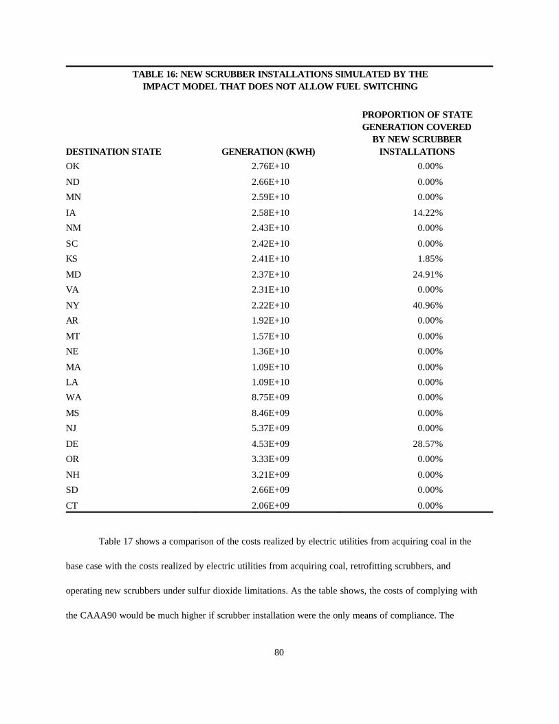
TABLE 16: NEW SCRUBBER INSTALLATIONS SIMULATED BY THEIMPACT MODEL THAT DOES NOT ALLOW FUEL SWITCHING

DESTINATION STATE GENERATION (KWH)

PROPORTION OF STATEGENERATION COVERED

BY NEW SCRUBBERINSTALLATIONS

80

OK 2.76E+10 0.00%

ND 2.66E+10 0.00%

MN 2.59E+10 0.00%

IA 2.58E+10 14.22%

NM 2.43E+10 0.00%

SC 2.42E+10 0.00%

KS 2.41E+10 1.85%

MD 2.37E+10 24.91%

VA 2.31E+10 0.00%

NY 2.22E+10 40.96%

AR 1.92E+10 0.00%

MT 1.57E+10 0.00%

NE 1.36E+10 0.00%

MA 1.09E+10 0.00%

LA 1.09E+10 0.00%

WA 8.75E+09 0.00%

MS 8.46E+09 0.00%

NJ 5.37E+09 0.00%

DE 4.53E+09 28.57%

OR 3.33E+09 0.00%

NH 3.21E+09 0.00%

SD 2.66E+09 0.00%

CT 2.06E+09 0.00%

Table 17 shows a comparison of the costs realized by electric utilities from acquiring coal in the

base case with the costs realized by electric utilities from acquiring coal, retrofitting scrubbers, and

operating new scrubbers under sulfur dioxide limitations. As the table shows, the costs of complying with

the CAAA90 would be much higher if scrubber installation were the only means of compliance. The

81

overall increase in costs to electric utilities is estimated at nearly 16 percent compared to an acquisition

cost increase of only 6 percent under the impact case where only switching is allowed. In actuality, some

utilities would switch coal, while others would install scrubbers. Thus, if the resources were available to

estimate the non-linear program that minimizes the total cost of compliance and coal acquisition, the

estimated total increase in compliance costs would be lower.

TABLE 17: COMPARISON OF COAL ACQUISITION COSTS FOR UTILITIESBETWEEN THE BASE CASE AND THE SCRUBBER RETROFIT CASE

(IMPACT CASE INCLUDES SCRUBBER RETROFIT COSTS)

DESTINATION STATE BASE (MILLION $) IMPACT (MILLION $) PERCENT CHANGE

OH 1,411.05 2,025.63 43.56%

MI 806.51 1,142.68 41.68%

IL 680.06 928.35 36.51%

WI 460.39 595.94 29.44%

MO 562.83 718.40 27.64%

IN 1,068.15 1,357.42 27.08%

KY 853.19 1,078.03 26.35%

NY 308.78 375.65 21.65%

PA 1,210.27 1,455.27 20.24%

TN 612.30 735.61 20.14%

FL 794.01 948.79 19.49%

GA 761.26 893.79 17.41%

DE 63.79 72.59 13.79%

IA 313.69 355.83 13.43%

MD 302.84 338.75 11.86%

WV 745.84 831.12 11.43%

AL 784.35 834.14 6.35%

KS 321.35 324.97 1.12%

TX 1,158.11 1,158.11 0.00%

NC 676.56 676.56 0.00%

WY 350.37 350.37 0.00%

AZ 420.30 420.30 0.00%

UT 344.92 344.92 0.00%

TABLE 17: COMPARISON OF COAL ACQUISITION COSTS FOR UTILITIESBETWEEN THE BASE CASE AND THE SCRUBBER RETROFIT CASE

(IMPACT CASE INCLUDES SCRUBBER RETROFIT COSTS)

DESTINATION STATE BASE (MILLION $) IMPACT (MILLION $) PERCENT CHANGE

82

CO 321.67 321.67 0.00%

OK 329.80 329.80 0.00%

ND 248.41 248.41 0.00%

MN 359.75 359.75 0.00%

NM 327.64 327.64 0.00%

SC 327.80 327.80 0.00%

VA 291.83 291.83 0.00%

AR 246.76 246.76 0.00%

NV 241.61 241.61 0.00%

MT 116.02 116.02 0.00%

NE 157.23 157.23 0.00%

MA 154.15 154.15 0.00%

LA 123.82 123.82 0.00%

WA 126.73 126.73 0.00%

MS 106.41 106.41 0.00%

NJ 72.67 72.67 0.00%

OR 53.22 53.22 0.00%

NH 47.40 47.40 0.00%

SD 36.33 36.33 0.00%

CT 28.16 28.16 0.00%

TOTAL 18,728.33 21,680.63 15.76%

83

CONCLUSION

This study has shown the great growth in coal production in the west. Since 1970, western coal

production has increased by more than 600 percent. Much of this increase has been due to an increased

desire for low sulfur coal by electric utilities. The Clean Air Act Ammendments of 1990 provide an

opportunity for a large increase in future coal production in the west. These amendments, which place a

cap on total sulfur dioxide emissions by U.S. utilities, allow electric utilities to use the least cost method of

reducing sulfur dioxide. This is in sharp contrast to previous environmental legislation, which has often

mandated scrubber installation. Because more than 80 percent of the nation's recoverable low sulfur

reserves are in the west, a great opportunity exists.

Linear programs were estimated, showing the large potential increases in annual western coal

production given the provisions of the Clean Air Act Ammendments of 1990. Because of a lack of

computer resources, a nonlinear program that minimizes total utility compliance costs while allowing

switching to low sulfur coal or scrubber installation could not be estimated. However, all of the data

required to estimate such a model have been collected and all of the programming required to estimate

such a model has been completed. Thus, when future computer resources become available, such a model

could be estimated.

While the linear programs estimated in this study show many of the expected changes with regard

to coal flows, they still do not come close to approximating reality. There are several problems with the

linear programs used in this study. First, they include many major simplifying assumptions such as an

exogenously-determined coal mine price, the use of only one transportation mode, the restriction of

demand points to electric utilities that already use coal as a primary fuel source, the elimination of exports

and imports from the model, and many others. These simplifications are made for purposes of tractability.

Second, they use data that is somewhat suspect. Many of the data items, particularly those related to coal

84

quality, appear to be inaccurate. However, the best known data sources are used. Finally, there may be

many other considerations by electric utilities in their fuel purchases, in addition to those modeled in the

linear programs. For example, many electric utility boilers in the U.S. were built with a particular fuel type

in mind. Changes in coal moisture content, ash content, and other volatile matter may have a large impact

on the efficiency with which coal is converted into electricity. However, no quantification of such effects

is known to exist.

Finally, the study shows that future changes in nationwide transportation rates could have a major

impact on regional coal production and coal market shares. Due to the west's lack of proximity to many

major utilities, transportation rates often consume a large portion of total acquisition costs by utilities in

purchasing western coal. To the extent that the increases in railroad efficiency that we have seen over

the past 15 years continue, western coal production should realize an even greater opportunity. However,

various trends affecting individual rates such as changes in railroad infrastructure, changes in the prices of

alternative fuels, and other factors will be equally important. This study also presents a model of rail rates,

showing the influences of costs and competitive factors in determining individual rates for coal.

85

86

87

REFERENCES

Ackerman and Hassler. Clean Coal/Dirty Air - or How the Clean Air Act Became aMultibillion-Dollar Bail-Out for High Sulfur Coal Producers and What Should Be Done About

It, New Haven, 1981.

Atkinson, Scott E. and Joe Kerkvliet. "Measuring the Multilateral Allocation of Rents: Wyoming Low Sulfur Coal, The Rand Journal of Economics, Autumn 1986.

Bryner, Gary C. Blue Skies, Green Politics - The Clean Air Act of 1990 and Its Implementation,Washington, D.C., 1995.

Decision Analysis Corporation of Virginia, "Regression Models for Analyzing Retrofit Flue Gas DesulfurizationUnitCostsandPerformance,"reportprepared fortheEnergyInformationAdministrationVienna,VA,May1993.

Dunbar, Frederick C. and Joyce S. Mehring, "Coal Rail Prices During Deregulation: A Hedonic Price Analysis," Logistics and Transportation Review, Vol. 26, No. 1, 1990.

Energy Information Administration. Acid Rain Compliance Strategies for the Clean Air ActAmendments of 1990, U.S. Department of Energy, Washington, D.C., 1994.

Energy Information Administration. Annual Outlook for U.S. Electric Power,U.S. Department ofEnergy, Washington, D.C., various years.

Energy Information Administration. Coal Production, U.S. Department of Energy, Washington,D.C., various years.

88

Energy Information Administration. Coal Distribution,U.S. Department of Energy, Washington, D.C., various years.

Energy Information Administration. Coal Transportation Rate Database,U.S. Department of Energy, Washington, D.C., 1991.

Energy Information Administration. Estimation of U.S. Coal Reserves by Coal Type,U.S. Departmentof Energy, Washington, D.C., 1989.

Energy Information Administration. Inventory of Power Plants in the United States 1993,U.S. Department of Energy, Washington, D.C., 1994.

Energy Information Administration. Resource Allocation and Mine Costing Model,U.S. Department of Energy, Washington, D.C., 1992.

Energy Information Administration. The U.S. Coal Industry, 1970-1990: Two Decades of Change,U.S. Department of Energy, Washington, D.C., 1993.

Energy Information Administration. Trends in Contract Coal Transportation 1979-1987,U.S.Department of Energy, Washington, D.C., 1991.

Energy Information Administration. "Annual Electric Generator Report, "U.S. Department of Energy, Washington, D.C., 1991-1993, available on the internet.

Energy Information Administration. "Monthly Power Plant Report "U.S. Department of Energy, Washington, D.C., 1991-1993, available on the internet.

Environmental Protection Agency, "40 CFR Parts 72 and 73 - Acid Rain Allowance Allocations and Reserves; Proposed Rules," Federal Register, 1992.

Fieldston Company, Fieldston Coal Transportation Manual, Washington, D.C., 1991.

Garrod, P.V. and W. Miklius. "Captive Shippers and the Success of Railroads in Capturing Monopoly Rent," Journal of Law and Economics, vol. 30, 1987.

Moody's Investor Service, Moody's Transportation Manual, New York, NY, 1995.

Rupinskas, Romas L. and Paul A. Hiller, "Considerations for Switching from High-Sulfur Coal to Low Sulfur Coal," Sargent and Lundy, paper presented at the 1992 International Joint PowerGeneration Conference and Exposition, Atlanta, GA, 1992.

Smith, James N. and Robert R. Rose. Rail Transport of Western Coal. Prepared for the WesternGovernor's Association, 1985.

U.S. Geological Survey. Coal Quality Database: Version 1.3, 1995.

89

Zimmerman, M.B. "Rent and Regulation in Unit Train Rate Determination" Bell Journal of Economics, 1979.

90

APPENDIX - SUPPLEMENTARY TABLES

91

92

TABLE A1: COAL FLOWS SIMULATED IN THE BASECASE

DESTINATIONSTATE ORIGIN STATE TONS (1,000)

SHARE OF DEST.STATE'S COAL REC.

AL WK 16,638.61 57.00%

AL TX 9,471.65 32.45%

AL TN 3,081.78 10.56%

AR TX 11,119.21 90.85%

AR OK 1,120.00 9.15%

AZ AZ 12,900.00 77.59%

AZ WY 3,726.83 22.42%

CO WY 10,505.05 61.76%

CO CO 6,503.77 38.24%

CT PA 762.75 100.00%

DE WV 1,642.05 100.00%

FL WK 24,389.17 91.94%

FL TX 2,137.87 8.06%

GA WK 19,958.35 86.30%

GA TN 3,168.25 13.70%

IA WY 8,253.94 57.26%

IA IA 6,160.59 42.74%

IL IL 10,650.08 45.47%

IL IN 8,654.71 36.95%

IL WK 3,482.02 14.87%

IL IA 634.58 2.71%

IN IN 41,257.01 97.63%

IN WK 999.62 2.37%

KS WY 14,688.97 98.63%

KS OK 203.85 1.37%

KY WK 19,740.32 59.44%

93

TABLE Al: COAL FLOWS SIMULATED IN THE BASE CASE

DESTINATIONSTATE ORIGIN STATE TONS (1,000)

SHARE OF DEST.STATE'S COAL REC.

KY EK 6,969.69 20.99%

KY IN 6,499.08 19.57%

LA TX 4,508.33 63.22%

LA LA 2,622.71 36.78%

MA WV 2,868.76 65.50%

MA WK 1,511.27 34.50%

MD WV 4,727.70 55.55%

MD MD 3,783.76 44.46%

MI WK 13,823.01 52.08%

MI IN 12,720.55 47.92%

MN WY 15,301.17 99.41%

MN IA 90.93 0.59%

MO WK 11,125.05 47.32%

MO WY 9,763.11 41.53%

MO IA 1,543.60 6.57%

MO OK 1,079.82 4.59%

MS TX 4,967.52 100.00%

MT MT 9,543.13 93.02%

MT WY 715.95 6.98%

NC VA 14,836.66 80.68%

NC WK 2,140.62 11.64%

NC EK 789.49 4.29%

NC WV 623.74 3.39%

ND ND 21,424.01 100.00%

NE WY 8,151.66 100.00%

NH WK 1,424.13 100.00%

NJ WV 1,198.53 62.27%

94

TABLE A1: COAL FLOWS SIMULATED IN THE BASECASE

DESTINATIONSTATE ORIGIN STATE TONS (1,000)

SHARE OF DEST.STATE'S COAL REC.

NJ PA 726.32 37.73%

NM WY 14,669.40 100.00%

NV WY 9,520.15 100.00%

NY PA 8,056.35 92.50%

NY WV 653.46 7.50%

OH OH 27,013.69 54.90%

OH WK 8,786.06 17.86%

OH EK 5,033.42 10.23%

OH IN 3,566.57 7.25%

OH PA 3,251.46 6.61%

OH WV 1,553.76 3.16%

OK TX 8,436.28 59.22%

OK OK 5,810.49 40.79%

OR WY 2,063.46 100.00%

PA PA 35,274.45 89.74%

PA MD 3,066.24 7.80%

PA WV 968.62 2.46%

SC WK 9,334.93 100.00%

SD WY 1,683.90 100.00%

TN WK 13,565.88 65.51%

TN TN 4,591.82 22.17%

TN VA 1,783.68 8.61%

TN EK 766.99 3.70%

TX TX 72,699.41 94.50%

TX WY 4,234.40 5.50%

UT UT 7,849.51 55.77%

UT WY 6,224.21 44.23%

95

TABLE A1: COAL FLOWS SIMULATED IN THE BASE CASEDESTINATION

STATE ORIGIN STATE TONS (1,000)SHARE OF DEST.

STATE'S COAL REC.VA WV 4,945.84 58.52%

VA VA 3,503.49 41.45%

VA WY 2.09 0.03%

WA WY 5,119.13 100.00%

WI WK 9,752.42 60.80%

WI IN 3,422.41 21.34%

WI WY 1,833.76 11.43%

WI IA 1,030.92 6.43%

WV WV 26,077.38 100.00%

WY WY 21,986.01 100.00%

96

TABLE A2: COAL FLOWS SIMULATED IN THE IMPACT CASE THAT DOES NOTALLOW SCRUBBER INSTALLATION

DESTINATIONSTATE

ORIGINSTATE TONS (1,000)

SHARE OF DEST.STATE'S COAL REC.

AL TX 12,789.77 45.09%

AL WK 5,484.25 19.33%

AL TN 5,156.54 18.18%

AL VA 3,525.55 12.43%

AL AR 1,410.22 4.97%

AR TX 12,608.91 100.00%

AZ AZ 12,900.00 77.59%

AZ WY 3,726.83 22.42%

CO WY 10,498.44 61.73%

CO CO 6,508.50 38.27%

CT W V 710.47 100.00%

DE WV 1;629.91 100.00%

FL WK 10,329.05 41.77%

FL VA 4,611.71 18.65%

FL TX 3,253.68 13.16%

FL AR 3,096.45 12.52%

FL EK 2,547.83 10.30%

FL OK 890.22 3.60%

GA VA 13,950.48 64.96%

GA WK 3,761.54 17.52%

GA EK 3,221.52 15.00%

GA TN 542.00 2.52%

IA WY 11,526.13 77.08%

IA IA 3,407.34 22.79%

IA OK 19.13 0.13%

IL WY 16,929.82 60.21%

IL IN 10,224.14 36.36%

97

TABLE A2: COAL FLOWS SIMULATED IN THE IMPACT CASE THAT DOES NOTALLOW SCRUBBER INSTALLATION

DESTINATIONSTATE

ORIGINSTATE TONS (1,000)

SHARE OF DEST.STATE'S COAL REC.

IL IA 512.51 1.82%

IL IL 450.23 1.60%

IN IN 28,531.14 67.47%

IN WK 9,996.64 23.64%

IN WY 1,388.98 3.29%

IN EK 1,358.54 3.21%

IN WV 1,013.20 2.40%

KS WY 15,007.38 100.00%

KY EK 16,366.05 51.31%

KY WK 14,330.80 44.93%

KY IN 1,197.05 3.75%

LA TX 4,483.20 63.09%

LA LA 2,622.71 36.91%

MA WV 3,864.96 100.00%

MD MD 4,633.78 54.23%

MD WV 3,910.94 45.77%

MI WV 15,064.21 59.49%

MI WY 6,649.48 26.26%

MI IN 3,609.03 14.25%

MN WY 15,301.17 99.34%

MN MT 102.29 0.66%

MO WY 20,803.20 78.34%

MO TX 3,964.75 14.93%

MO WK 1,069.08 4.03%

MO OK 717.31 2.70%

MS TX 5,045.81 100.00%

MT MT 10,160.42 100.00%

98

TABLE A2: COAL FLOWS SIMULATED IN THE IMPACT CASE THAT DOES NOTALLOW SCRUBBER INSTALLATION

DESTINATIONSTATE

ORIGINSTATE TONS (1,000)

SHARE OF DEST.STATE'S COAL REC.

NC VA 17,546.51 94.80%

NC W V 963.09 5.20%

ND ND 21,148.04 100.00%

NE WY 8,151.66 100.00%

NH W V 1,154.91 100.00%

NJ W V 1,868.59 100.00%

NM WY 14,669.40 100.00%

NV WY 9,520.15 100.00%

NY WV 4,190.16 48.68%

NY PA 2,280.35 26.50%

NY WK 2,136.32 24.82%

OH W V 39,826.46 90.75%

OH EK 3,295.47 7.51%

OH VA 745.82 1.70%

OH WY 18.55 0.04%

OK TX 10,332.03 68.44%

OK OK 4,765.00 31.56%

OR WY 2,063.46 100.00%

PA PA 18,371.76 48.54%

PA W V 16,460.25 43.49%

PA 3,017.02 7.97%

SC VA 6,927.64 79.51%

SC EK 843.52 9.68%

SC WV 810.45 9.30%

SC WK 131.70 1.51%

SD WY 1,683.90 100.00%

TN TN 7,199.46 31.85%

99

TABLE A2: COAL FLOWS SIMULATED IN THE IMPACT CASE THAT DOES NOTALLOW SCRUBBER INSTALLATION

DESTINATIONSTATE

ORIGINSTATE TONS (1,000)

SHARE OF DEST.STATE'S COAL REC.

TN TX 6,693.69 29.61%

TN WK 6,539.98 28.93%

TN VA 1,797.58 7.95%

TN EK 372.58 1.65%

TX TX 72,441.80 94.48%

TX WY 4,234.40 5.52%

UT UT 7,849.51 55.77%

UT WY 6,224.21 44.23%

VA WV 6,585.54 81.78%

VA VA 1,464.71 18.19%

VA WY 2.09 0.03%

WA WY 5,119.13 100.00%

WI WY 15,165.47 79.46%

WI IA 3,780.09 19.81%

WI WV 139.03 0.73%

WV WV 24,861.94 100.00%

WY WY 21,986.01 100.00%

100

TABLE A3: COAL PRODUCTION SIMULATED BY MINIMIZING TRANSPORT

COSTS SUBJECT TO SULFUR LIMITATIONS, WITH A 20 PERCENT

OVERALL INCREASE IN RAIL RATES

STATE TONS (1,000) MARKET SHARE

WV 135,698 18.84%

WY 133,608 18.55%

TX 117,127 16.26

WKY 51,846 7.20%

VA 50,570 7.02%

IN 48,690 6.76%

PA 29,925 4.16%

EKY 26,465 3.67%

ND 21,341 2.96%

UT 17,650 2.45%

AZ 12,900 1.79%

TN 12,898 1.79%

IL 12,033 1.67%

OK 10,348 1.44%

MT 10,160 1.41%

CO 8,800 1.22%

IA 5,768 0.80%

AR 4,507 0.63%

MD 4,380 0.61%

LA 2,623 0.36%

NM 2,292 0.32%

OH 592 0.08%94

101

TABLE A4: COAL PRODUCTION SIMULATED BY MINIMIZING TRANSPORT

COSTS SUBJECT TO SULFUR LIMITATIONS, WITH A 20 PERCENT

OVERALL REDUCTION IN RAIL RATES

STATE TONS (1,000) MARKET SHARE

WY 255,070 33.26%

TX 142,573 18.59%

WV 90,347 11.78%

WKY 55,605 7.25%

VA 49,350 6.43%

IN 32,113 4.19%

EKY 28,394 3.70%

ND 21,341 2.78%

PA 17,970 2.34%

AZ 12,900 1.68%

TN 12,898 1.68%

MD 11,230 1.46%

MT 9,730 1.27%

IA 8,882 1.16%

UT 7,850 1.02%

OK 5,689 0.74%

LA 2,623 0.34%

AR 2,253 0.29%

CO 179 0.02%

102

TABLE A5: COAL PRODUCING STATES AND COUNTIES INCLUDEDIN THE LINEAR PROGRAMMING MODELS

COAL PRODUCING STATE COAL PRODUCING COUNTY

AL BIBB

AL BLOUNT

AL CULLMAN

AL FAYETTE

AL JEFFERSON

AL MARION

AL SHELLBY

AL ST CLAIR

AL TUSCALOOSA

AL WALKER

AL WINSTON

AR JOHNSON

AR SALINE

AR SEBASTIAN

AZ NAVAJO

CA AMADOR

CO DELTA

CO FREMONT

CO GARFIELD

CO GARFIELD

CO GUNNISON

CO JACKSON

CO LA PLATA

CO LAS ANIMAS

CO MOFFAT

CO MONTROSE

CO PITKIN

TABLE A5: COAL PRODUCING STATES AND COUNTIES INCLUDEDIN THE LINEAR PROGRAMMING MODELS

COAL PRODUCING STATE COAL PRODUCING COUNTY

103

CO RIO BLANCO

CO ROUTT

CO WELD

IA MARION

IA MONROE

IL CHRISTIAN

IL CLINTON

IL DOUGLAS

IL EDGAR

IL FRANKLIN

IL FULTON

IL GALLATIN

IL HAMILTON

IL JACKSON

IL JEFFERSON

IL LOGAN

IL MACOUPIN

IL MCDONOUGH

IL PERRY

IL RANDOLPH

IL SALINE

IL SANGAMON

IL SCHUYLER

IL ST CLAIR

IL WABASH

IL WASHINGTON

IL WHITE

TABLE A5: COAL PRODUCING STATES AND COUNTIES INCLUDEDIN THE LINEAR PROGRAMMING MODELS

COAL PRODUCING STATE COAL PRODUCING COUNTY

104

IL WILLIAMSON

IN CLAY

IN DAVIESS

IN DUBOIS

IN GIBSON

IN GREENE

IN KNOX

IN MARTIN

IN OWEN

IN PERRY

IN PIKE

IN SPENCER

IN SULLIVAN

IN VERMILLION

IN VIGO

IN WARRICK

KS CRAWFORD

KS LINN

KY BELL

KY BOYD

KY BREATHITT

KY BUTLER

KY CALDWELL

KY CARTER

KY CHRISTIAN

KY CLAY

KY CLINTON

TABLE A5: COAL PRODUCING STATES AND COUNTIES INCLUDEDIN THE LINEAR PROGRAMMING MODELS

COAL PRODUCING STATE COAL PRODUCING COUNTY

105

KY DAVIESS

KY EDMONSON

KY ELLIOTT

KY FLOYD

KY GREENUP

KY HANCOCK

KY HARLAN

KY HENDERSON

KY HOPKINS

KY JACKSON

KY JOHNSON

KY KNOTT

KY KNOX

KY LAUREL

KY LAWRENCE

KY LEE

KY LESLIE

KY LETCHER

KY MAGOFFIN

KY MARTIN

KY MCCREARY

KY MCLEAN

KY MORGAN

KY MUHLENBERG

KY OHIO

KY OWSLEY

KY PERRY

TABLE A5: COAL PRODUCING STATES AND COUNTIES INCLUDEDIN THE LINEAR PROGRAMMING MODELS

COAL PRODUCING STATE COAL PRODUCING COUNTY

106

KY PIKE

KY PULASKI

KY UNION

KY WAYNE

KY WEBSTER

KY WHITLEY

KY WOLFE

LA DE SOTO

LA RED RIVER

MD ALLEGANY

MD GARRETT

MO BARTON

MO BATES

MO PUTNAM

MO RALLS

MO RANDOLPH

MO VERNON

MT BIG HORN

MT MUSSELSHELL

MT RICHLAND

MT ROSEBUD

ND BOWMAN

ND MCLEAN

ND MERCER

ND OLIVER

ND STARK

ND WILLIAMS

TABLE A5: COAL PRODUCING STATES AND COUNTIES INCLUDEDIN THE LINEAR PROGRAMMING MODELS

COAL PRODUCING STATE COAL PRODUCING COUNTY

107

NM COLFAX

NM MCKINLEY

NM SAN JUAN

OH ATHENS

OH BELMONT

OH CARROLL

OH COLUMBIANA

OH COSHOCTON

OH GALLIA

OH GUERNSEY

OH HARRISON

OH HOCKING

OH HOLMES

OH JACKSON

OH JEFFERSON

OH LAWRENCE

OH MAHONING

OH MEIGS

OH MONROE

OH MUSKINGUM

OH NOBLE

OH PERRY

OH STARK

OH TUSCARAWAS

OH VINTON

OH WASHINGTON

OK COAL

TABLE A5: COAL PRODUCING STATES AND COUNTIES INCLUDEDIN THE LINEAR PROGRAMMING MODELS

COAL PRODUCING STATE COAL PRODUCING COUNTY

108

OK CRAIG

OK HASKELL

OK LATIMER

OK LE FLORE

OK MCINTOSH

OK MUSKOGEE

OK NOWATA

OK OKMULGEE

OK ROGERS

OK WAGONER

PA ALLEGHENY

PA ARMSTRONG

PA BEAVER

PA BEDFORD

PA BLAIR

PA BUTLER

PA CAMBRIA

PA CARBON

PA CENTRE

PA CLARION

PA CLEARFIELD

PA CLINTON

PA COLUMBIA

PA ELK

PA FAYETTE

PA FULTON

PA GREENE

TABLE A5: COAL PRODUCING STATES AND COUNTIES INCLUDEDIN THE LINEAR PROGRAMMING MODELS

COAL PRODUCING STATE COAL PRODUCING COUNTY

109

PA INDIANA

PA JEFFERSON

PA LACKAWANNA

PA LAWRENCE

PA LUZERNE

PA LYCOMING

PA MERCER

PA NORTHUMBERLAND

PA SCHUYLKILL

PA SOMERSET

PA SULLIVAN

PA TIOGA

PA VENANGO

PA WASHINGTON

PA WESTMORELAND

TN ANDERSON

TN BLEDSOE

TN CAMPBELL

TN CLAIBORNE

TN CUMBERLAND

TN FENTRESS

TN GRUNDY

TN MARION

TN MORGAN

TN RHEA

TN SCOTT

TN SEQUATCHIE

TABLE A5: COAL PRODUCING STATES AND COUNTIES INCLUDEDIN THE LINEAR PROGRAMMING MODELS

COAL PRODUCING STATE COAL PRODUCING COUNTY

110

TX ATASCOSA

TX BASTROP

TX FREESTONE

TX GRIMES

TX HARRISON

TX HOPKINS

TX LEON

TX MILLAM

TX PANOLA

TX RUSK

TX TITUS

TX WEBB

UT CARBON

UT EMERY

UT SEVIER

UT SUMMIT

VA BUSHANAN

VA DICKENSON

VA LEE

VA RUSSELL

VA SCOTT

VA TAZEWELL

VA WISE

WA KING

WA LEWIS

WA THURSTON

WV BARBOUR

TABLE A5: COAL PRODUCING STATES AND COUNTIES INCLUDEDIN THE LINEAR PROGRAMMING MODELS

COAL PRODUCING STATE COAL PRODUCING COUNTY

111

WV BOONE

WV BRAXTON

WV BROOKE

WV CLAY

WV FAYETTE

WV GILMER

WV GRANT

WV GREENBRIER

WV HARRISON

WV KANAWHA

WV LEWIS

WV LINCOLN

WV LOGAN

WV MARION

WV MARSHALL

WV MASON

WV MCDOWELL

WV MERCER

WV MINERAL

WV MINGO

WV MONOGALIA

WV NICHOLAS

WV OHIO

WV PRESTON

WV RALEIGH

WV RANDOLPH

WV TAYLOR

TABLE A5: COAL PRODUCING STATES AND COUNTIES INCLUDEDIN THE LINEAR PROGRAMMING MODELS

COAL PRODUCING STATE COAL PRODUCING COUNTY

112

WV TUCKER

WV UPSHUR

WV WAYNE

WV WEBSTER

WV WYOMING

WY CAMPBELL

WY CARBON

WY CONVERSE

WY HOT SPRINGS

WY LINCOLN

WY SHERIDAN

WY SWEETWATER

113

TABLE A6: STATES AND COUNTIES WITH COAL CONSUMING ELECTRIC UTILITIES

DESTINATION STATE DESTINATION COUNTY

AL COLBERT

AL COVINGTON

AL ETOWAH

AL GREENE

AL JACKSON

AL JEFFERSON

AL MOBILE

AL SHELBY

AL WALKER

AL WASHINGTON

AR BENTON

AR INDEPENDENCE

AZ APACHE

AZ COCHISE

AZ COCONINO

AZ NAVAJO

AZ PIMA

CO ADAMS

CO BOULDER

CO DENVER

CO EL PASO

CO FREMONT

CO LARIMER

CO LAS ANIMAS

CO MESA

CO MOFFAT

CO MONTROSE

TABLE A6: STATES AND COUNTIES WITH COAL CONSUMING ELECTRIC UTILITIES

DESTINATION STATE DESTINATION COUNTY

114

CO MORGAN

CO PUEBLO

CO ROUTT

CT FAIRFIELD

CT HARTFORD

DE NEW CASTLE

DE SUSSEX

FL ALACHUA

FL BAY

FL CITRUS

FL DUVAL

FL ESCAMBIA

FL HILLSBOROUGH

FL JACKSON

FL ORANGE

FL POLK

FL PUTNAM

GA BARTOW

GA BIBB

GA CHATHAM

GA COBB

GA COWETA

GA DOUGHERTY

GA EFFINGHAM

GA FLOYD

GA HEARD

GA MONROE

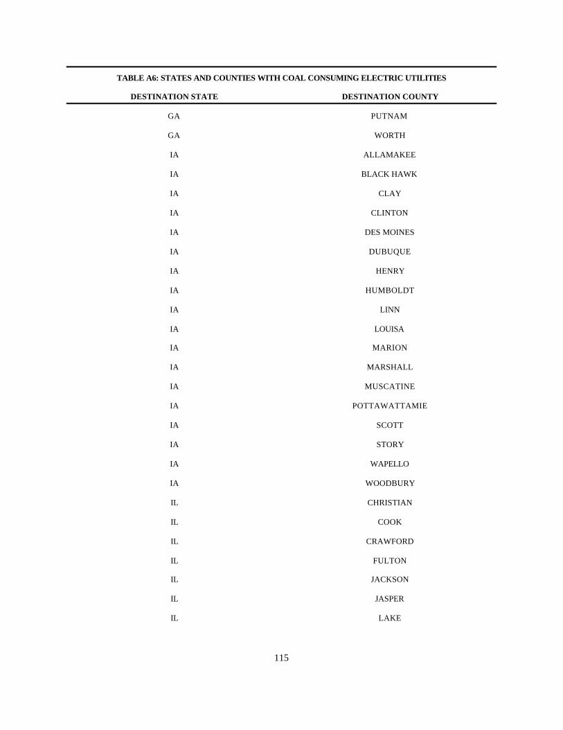
TABLE A6: STATES AND COUNTIES WITH COAL CONSUMING ELECTRIC UTILITIES

DESTINATION STATE DESTINATION COUNTY

115

GA PUTNAM

GA WORTH

IA ALLAMAKEE

IA BLACK HAWK

IA CLAY

IA CLINTON

IA DES MOINES

IA DUBUQUE

IA HENRY

IA HUMBOLDT

IA LINN

IA LOUISA

IA MARION

IA MARSHALL

IA MUSCATINE

IA POTTAWATTAMIE

IA SCOTT

IA STORY

IA WAPELLO

IA WOODBURY

IL CHRISTIAN

IL COOK

IL CRAWFORD

IL FULTON

IL JACKSON

IL JASPER

IL LAKE

TABLE A6: STATES AND COUNTIES WITH COAL CONSUMING ELECTRIC UTILITIES

DESTINATION STATE DESTINATION COUNTY

116

IL MADISON

IL MASON

IL MASSAC

IL MONTGOMERY

IL MORGAN

IL PEORIA

IL PIKE

IL PUTNAM

IL RANDOLPH

IL SANGAMON

IL TAZEWELL

IL VERMILLION

IL WILL

IL WILLIAMSON

IN CASS

IN DEARBORN

IN DUBOIS

IN FLOYD

IN GIBSON

IN HAMILTON

IN JASPER

IN JEFFERSON

IN KNOX

IN LA PORTE

IN LAKE

IN MARION

IN MIAMI

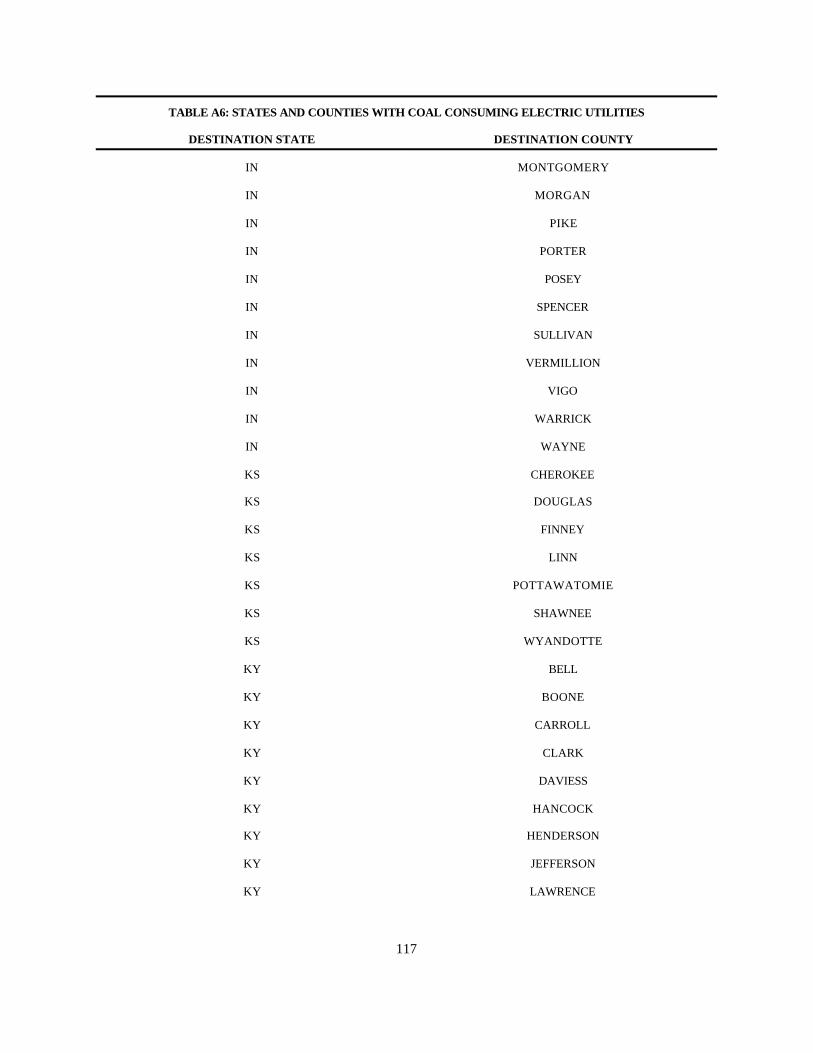
TABLE A6: STATES AND COUNTIES WITH COAL CONSUMING ELECTRIC UTILITIES

DESTINATION STATE DESTINATION COUNTY

117

IN MONTGOMERY

IN MORGAN

IN PIKE

IN PORTER

IN POSEY

IN SPENCER

IN SULLIVAN

IN VERMILLION

IN VIGO

IN WARRICK

IN WAYNE

KS CHEROKEE

KS DOUGLAS

KS FINNEY

KS LINN

KS POTTAWATOMIE

KS SHAWNEE

KS WYANDOTTE

KY BELL

KY BOONE

KY CARROLL

KY CLARK

KY DAVIESS

KY HANCOCK

KY HENDERSON

KY JEFFERSON

KY LAWRENCE

TABLE A6: STATES AND COUNTIES WITH COAL CONSUMING ELECTRIC UTILITIES

DESTINATION STATE DESTINATION COUNTY

118

KY MASON

KY MCCRACKEN

KY MERCER

KY MUHLENBERG

KY OHIO

KY PULASKI

KY TRIMBLE

KY WEBSTER

KY WOODFORD

LA CALCASIEU

LA DE SOTO

LA RAPIDES

MA BRISTOL

MA ESSEX

MA HAMPDEN

MD ANNE ARUNDEL

MD BALTIMORE

MD CHARLES

MD MONTGOMERY

MD PRINCE GEORGES

MD WASHINGTON

MI BARAGA

MI BAY

MI BRANCH

MI CHARLEVOIX

MI DELTA

MI EATON

TABLE A6: STATES AND COUNTIES WITH COAL CONSUMING ELECTRIC UTILITIES

DESTINATION STATE DESTINATION COUNTY

119

MI GRAND TRAVERSE

MI HILLSDALE

MI HURON

MI INGHAM

MI MARQUETTE

MI MONROE

MI MUSKEGON

MI OTTAWA

MI ST CLAIR

MI WAYNE

MN BROWN

MN CHIPPEWA

MN CLAY

MN DAKOTA

MN HENNEPIN

MN ITASCA

MN KANDIYOHI

MN MARTIN

MN MOWER

MN OLMSTED

MN OTTER TAIL

MN RAMSEY

MN SHERBURNE

MN ST LOUIS

MN WASHINGTON

MO BOONE

MO BUCHANAN

TABLE A6: STATES AND COUNTIES WITH COAL CONSUMING ELECTRIC UTILITIES

DESTINATION STATE DESTINATION COUNTY

120

MO CLAY

MO FRANKLIN

MO GREENE

MO HENRY

MO JACKSON

MO JASPER

MO JEFFERSON

MO LIVINGSTON

MO NEW MADRID

MO OSAGE

MO PLATTE

MO RANDOLPH

MO SALINE

MO SCOTT

MO ST LOUIS

MO ST CHARLES

MS HARRISON

MS JACKSON

MS LAMAR

MS LEFLORE

MT RICHLAND

MT ROSEBUD

MT YELLOWSTONE

NC BUNCOMBE

NC CATAWBA

NC CHATHAM

NC CLEVELAND

TABLE A6: STATES AND COUNTIES WITH COAL CONSUMING ELECTRIC UTILITIES

DESTINATION STATE DESTINATION COUNTY

121

NC GASTON

NC NEW HANOVER

NC PERSON

NC ROBESON

NC ROCKINGHAM

NC ROWAN

NC STOKES

NC WAYNE

ND MCHENRY

ND MCLEAN

ND MERCER

ND MORTON

ND OLIVER

NE ADAMS

NE DODGE

NE DOUGLAS

NE HALL

NE LANCASTER

NE LINCOLN

NE OTOE

NH MERRIMACK

NH ROCKINGHAM

NJ CAPE MAY

NJ CUMBERLAND

NJ HUDSON

NJ MERCER

NJ SALEM

TABLE A6: STATES AND COUNTIES WITH COAL CONSUMING ELECTRIC UTILITIES

DESTINATION STATE DESTINATION COUNTY

122

NM COLFAX

NM MCKINLEY

NM SAN JUAN

NV CLARK

NV HUMBOLDT

NY BROOME

NY CHAUTAUQUA

NY CHENANGO

NY ERIE

NY NIAGARA

NY ORANGE

NY ROCKLAND

NY STEUBEN

NY TOMPKINS

NY YATES

OH ADAMS

OH ASHTABULA

OH AUGLAIZE

OH BELMONT

OH BUTLER

OH CLERMONT

OH COSHOCTON

OH CUYAHOGA

OH FRANKLIN

OH GALLIA

OH HAMILTON

OH JEFFERSON

TABLE A6: STATES AND COUNTIES WITH COAL CONSUMING ELECTRIC UTILITIES

DESTINATION STATE DESTINATION COUNTY

123

OH LAKE

OH LORAIN

OH LUCAS

OH MAHONING

OH MIAMI

OH MONTGOMERY

OH MORGAN

OH PICKAWAY

OH RICHLAND

OH SUMMIT

OH TUSCARAWAS

OH WASHINGTON

OH WAYNE

OK CHOCTAW

OK MAYES

OK MUSKOGEE

OK NOBLE

OK ROGERS

OR MORROW

PA ALLEGHENY

PA ARMSTRONG

PA BEAVER

PA BERKS

PA CHESTER

PA CLEARFIELD

PA DELAWARE

PA GREENE

TABLE A6: STATES AND COUNTIES WITH COAL CONSUMING ELECTRIC UTILITIES

DESTINATION STATE DESTINATION COUNTY

124

PA INDIANA

PA LANCASTER

PA LAWRENCE

PA LUZERNE

PA MONTOUR

PA NORTHAMPTON

PA SNYDER

PA WARREN

PA WASHINGTON

PA YORK

SC AIKEN

SC ANDERSON

SC BERKELEY

SC COLLETON

SC DARLINGTON

SC GEORGETOWN

SC HORRY

SC LEXINGTON

SC RICHLAND

SD GRANT

SD LAWRENCE

SD PENNINGTON

TN ANDERSON

TN HAWKINS

TN HUMPHREYS

TN RHEA

TN ROANE

TABLE A6: STATES AND COUNTIES WITH COAL CONSUMING ELECTRIC UTILITIES

DESTINATION STATE DESTINATION COUNTY

125

TN SHELBY

TN STEWART

TN SUMNER

TX ATASCOSA

TX BEXAR

TX FAYETTE

TX FORT BEND

TX FREESTONE

TX GOLIAD

TX GRIMES

TX HARRISON

TX LAMB

TX LIMESTONE

TX MILAM

TX POTTER

TX ROBERTSON

TX RUSK

TX TITUT

TX WILBARGER

UT CARBON

UT EMERY

UT MILLARD

UT SALT LAKE

UT UINTAH

UT UTAH

VA ALEXANDRIA

VA CHESAPEAKE

TABLE A6: STATES AND COUNTIES WITH COAL CONSUMING ELECTRIC UTILITIES

DESTINATION STATE DESTINATION COUNTY

126

VA CHESTERFIELD

VA FLUVANNA

VA GILES

VA PRINCE WILLIAM

VA RUSSELL

VA YORK

WA LEWIS

WI ASHLAND

WI BROWN

WI BUFFALO

WI COLUMBIA

WI DANE

WI GRANT

WI KENOSHA

WI MANITOWOC

WI MARATHON

WI MILWAUKEE

WI OZAUKEE

WI ROCK

WI SHEBOYGAN

WI VERNON

WI WINNEBAGO

WI WOOD

WV GRANT

WV HARRISON

WV KANAWHA

WV MARION

TABLE A6: STATES AND COUNTIES WITH COAL CONSUMING ELECTRIC UTILITIES

DESTINATION STATE DESTINATION COUNTY

127

WV MARSHALL

WV MASON

WV MONONGALIA

WV PLEASANTS

WV PRESTON

WV PUTNAM

WY CAMPBELL

WY CONVERSE

WY LINCOLN

WY PLATTE

WY SWEETWATER

WY WESTON