THE IMPACTS OF REMOVAL OF FARM-FUEL TAX EXEMPTION ON CO2

EMISSIONS FROM PRAIRIE AGRICULTURE

Varghese Manaloor Augustana Faculty

University of Alberta

Abstract

The structural and technological changes that have taken place over the past several decades have resulted in an increased use of direct and indirect energy inputs in agriculture in the Canadian Prairies. Under the Kyoto protocol, which came into effect internationally on February 16, 2005, Canada has made a commitment to the international community to stabilize CO2 emissions at 6 percent below 1990 levels. The target is supposed to be reached by 2008 and maintained through 2012. This paper investigates the impacts of the removal of the current provincial farm fuel tax exemption programs on energy-use patterns, CO2 emissions, net farm income, and government tax revenue. To analyze these impacts, the elasticities of substitution between energy and other farm inputs were used. The elasticity estimates were used to look at changes in farm output and resulting changes in net farm income and CO2 emissions from the agricultural sector.

Varghese Manaloor Associate Professor Augustana Faculty

University of Alberta 4901-46th Avenue Camrose, Alberta Canada, T4V 2R3

Phone # (780) 679-1191 Fax # (780) 679-1129

E-mail: varghese.manaloor@ualberta.ca

Introduction

Interest in agricultural energy use in the late 1970s occurred mainly because of rising energy prices. During the 1990s environmental concerns were added on to the debate. Increased crop production in Canada, as in the rest of the developed world, has been achieved through technical change, that is, through the expanded use of increasingly sophisticated inputs, such as farm machinery, fertilizers, herbicides, and irrigation, and through the clearing of new lands, which all involved the use of commercial energy. And, the substitution of capital for labour has increased the reliance of agriculture on non-renewable energy resources. The largest anthropogenic source of carbon dioxide (CO2) emissions is the combustion of fossil fuels for energy generation. Agriculture contributes to increased CO2 concentrations in the atmosphere through the use of inputs such as fossil fuels, fertilizers, pesticides, and other energy-based inputs. The concentration of CO2 and other green house gases (GHG) in the atmosphere has been rising from historical levels, primarily due to fossil-fuel burning and land-use changes. Under the Kyoto protocol, which came into effect internationally on February 16, 2005, Canada has made a commitment to the international community to stabilize CO2 emissions at 6 percent below 1990 levels. The Climate Change Task Group (CCTG) identified options to achieve this goal in its “Report on Options for Canada's National Action Program on Climate Change” (1994). The CCTG recommended that voluntary measures should be given priority, yet acknowledged that the option for stabilization may have to involve the use of economic instruments, such as energy taxes, carbon taxes, and the removal or redirection of subsidies. These measures are proposed as tools to change the current incentive structure and, hence, the energy-use patterns. Olsen et al (2002) study points to the fact that GHG emissions in Canada have steadily increased in Canada since 1990. The AAFC (Agriculture and Agri-food Canada) study in 2000 looked at various options to reduce GHG. All measures were of bio-physical nature. Any change in taxes or subsidies that targets energy use is expected to alter the consumption patterns via their impact on relative prices. This, in turn, would affect production costs and input allocation decisions in agriculture. The magnitude of these impacts depends upon the substitution possibilities between energy, energy-based, and non-energy inputs that are employed in agricultural production. An analysis of the impacts of price changes on agricultural energy use requires information on substitution possibilities amongst the factors of production, and on own- and cross-price elasticities of demand for each input Carraro and Siniscalco (1994) have shown that taxation alone would not have a significant impact on CO2 emissions because of the low elasticities of substitution between energy and other inputs. In Canada, research on substitution of non-energy for energy inputs in agriculture has been rather limited. In 1982, Lopez and Tung estimated the elasticities of substitution between energy and non-energy inputs. Their results, however, are based on aggregate data (1961-79) for the entire country, and have limited use for policy analysis given the diverse nature of production, especially between Central and Western Canada. The regional differences in resource endowments resulted in different directions in technical change. In the Prairies, the direction has been machinery-using, that is, substituting capital for the scarce factor labour, while in Central Canada energy-based inputs such as fertilizers substituted for the scarce factor land (Karagiannis and Furtan 1990). The result has been different factor intensities in agriculture: high direct energy intensity in the Prairies and high indirect energy intensity in Central Canada. Yildirim and Manaloor (1995) estimated the elasticities of substitution and own and cross price elasticities for Western Canadian Agriculture1. This study examines the sustainability of the removal of provincial farm-fuel tax rebate/exemption programs in the Prairies. An assessment of the economic and environmental sustainability of a particular policy option requires a measure of the costs and benefits associated with this option. The environmental benefits of the policy are evaluated in terms of their ability to reduce total CO2 emissions from prairie agriculture. Economic costs and benefits are

1 The paper uses information available in research reports by Yildirim and Manaloor (1995) and Yildirim, Manaloor, and White (1995)

measured in terms of predicted changes in net farm income and in government revenue. Although the predicted changes in input demands will affect other sectors of the economy, these impacts cannot be analyzed within a partial-equilibrium framework. The cost-benefit calculations will therefore be limited to changes in net farm income and government tax revenue from the agricultural sector. Energy Use Patterns in Prairie Agriculture Energy use in agriculture can be divided into two categories: direct energy and indirect energy. Direct energy, the energy required to power machinery and to heat buildings, includes refined petroleum products, natural gas, and electricity. Indirect energy is the energy embodied in other factors of production, such as fertilizers, pesticides, and herbicides. In this study, direct energy includes fossil fuels, electricity, and natural gas. The organization of production in the three Prairie Provinces differs in each; the proportion of cash receipts from crop and livestock enterprises shows the diverse nature of their agricultural production. Table 1 shows the percentage share of crop and livestock in total cash receipts. Table 1 Farm Cash Receipts, 2003 (in ‘000 $) Saskatchewan Manitoba Alberta Total crops 2,743,907 1,678,231 1,898,395 % of Total (A) 67% 52% 34% Total Livestock 1,337,500 1,553,003 3,753,072 % of Total (A) 33% 48% 66% Total Payments 1,601,072 308,117 1,362,045 Total Receipts 5,682,479 3,539,351 7,013,512 Total Receipt less Payments (A) 4,081,407 3,231,234 5,651,467

Source: Statistics Canada, Catalogue No. 21-001-XIE, November, 2004

In 2003, 67 percent of total farm cash receipts in Saskatchewan were from crop

production. In Alberta, approximately 66 percent of total farm cash receipts originated from the livestock sector, whereas in Manitoba, crop and livestock receipts were each about 50 percent of the total farm cash receipts. The differences in output mix have implications for both the types and the quantities of energy used in production-related activities in each province. For example, diesel and indirect energy use are associated more with crop production, while electricity and natural gas are used mostly in the livestock sector. Specifically, gasoline and diesel are primarily used for farm machinery operations and transportation, while natural gas and electricity are mostly used for heating farm buildings and barns, crop drying, and irrigation. The share of energy inputs in expenditures in the three provinces provides an indication of their relative importance. Table 2 shows the expenditures on energy inputs in Saskatchewan, Manitoba, and Alberta. In Saskatchewan and Manitoba, combined expenditures on direct and indirect energy, in 2003, were respectively 37% and 30% of total farm operating expenses. Alberta’s share was approximately 25%. Table 2 Expenditure on Energy Inputs on Saskatchewan, Manitoba, and Alberta Farms, 2003 Saskatchewan Manitoba Alberta

Million $ Percent of TOE Million $

Percent of TOE Million $

Percent of TOE

Electricity 97.129 1.93 61.809 2.04 144.99 2.30 Heating Fuel 33.634 0.67 27.844 0.92 73.991 1.17 Machinery Fuel 401.124 7.95 184.494 6.09 368.828 5.85 Sub-total: Direct Energy Inputs 531.887 10.55 274.147 9.05 587.809 9.33 Fertilizer 737.593 14.62 388.539 12.82 570.352 9.05 Pesticides 614.882 12.19 241.656 7.97 321.521 5.10 Sub-Total: Indirect Energy Inputs 1352.475 26.82 630.195 20.79 891.873 14.16 Total Operating Expenses (TOE) 5043.642 100.00 3030.631 100.00 6300.494 100.00

Source: CANSIM (2005) Table Number 20005 Direct Energy Use Petroleum products and electricity constitute the bulk of direct energy use in prairie agriculture. Table 3 shows the quantities of the different types of energy used in prairie agriculture in 2003. The data reported in this section reflect the Statistics Canada estimates and do not include residential energy use in farms. Table 3 Energy Use in Agriculture, by Type of Energy, 2003 Type Alberta Saskatchewan ManitobaTotal Refined Petroleum Products ('000 Cu M) 1023.1 749.1 431.7 Gasoline ('000 Cu M) 428.2 211.7 148.2 Diesel ('000 Cu M) 590.1 530.8 280.7 Kerosene & Stove Oil ('000 Cu M) 0.5 1.9 1.3 Light Fuel Oil ('000 Cu M) 4.5 3.3 1.5 Lub Oil & Grease ('000 Cu M) n/a n/a n/a Natural Gas (GL) 127 132.7 1.5 Electricity (GWH) 1928.1 1441.9 1618.4

Source: CANSIM II (2005) Note: Cu M= cubic meters, GL= GigaLitres, and GWH= Gigawatt hours.

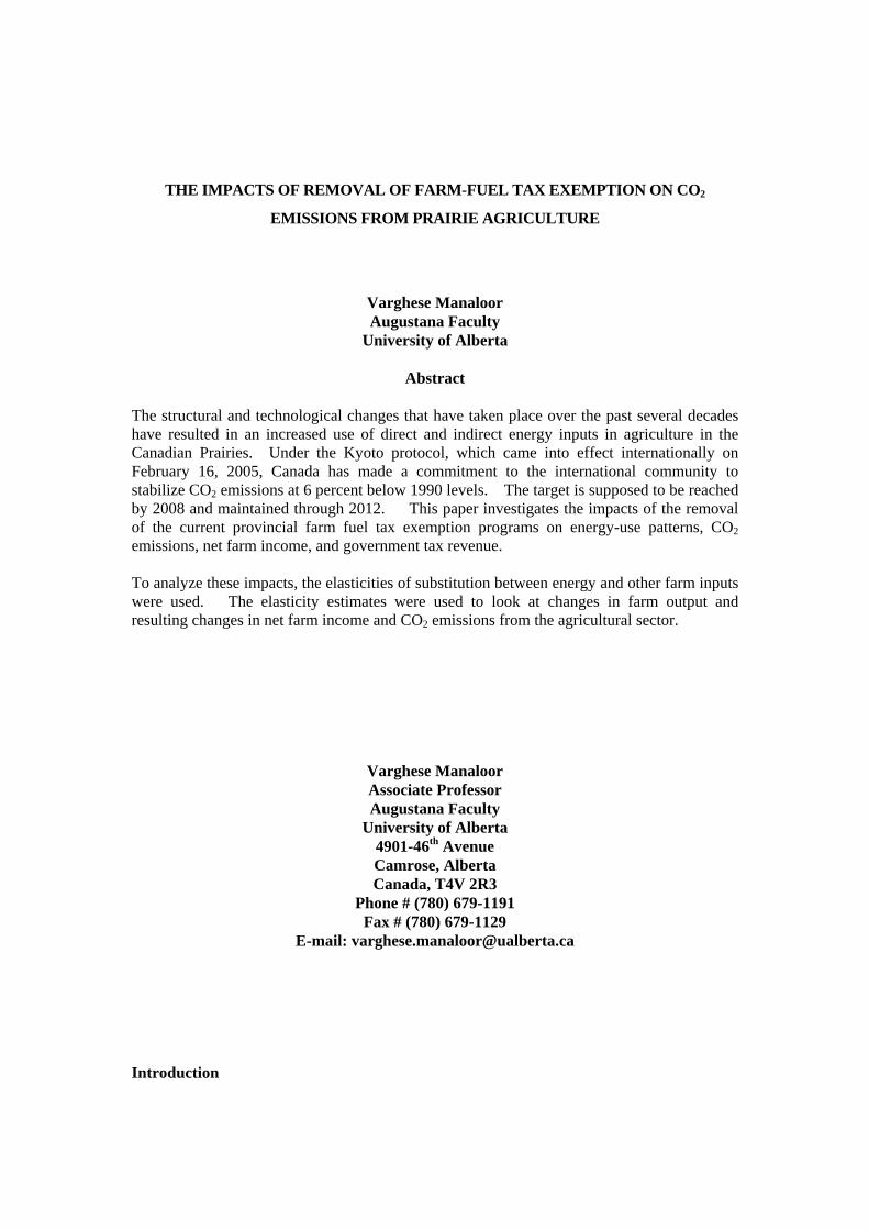
Table 4 shows the direct energy used (in TeraJoules) in prairie agriculture over the past 10 years. Conversions from energy quantities to standard energy measures were made based on the following assumptions: the energy content of all refined petroleum products is 38,680 KJ per litre, natural gas contains 38,020 KJ per m3, and electricity contains 3.6 TeraJoules per GWh (Statistics Canada, Energy Statistics Handbook, 1994). The shares of different types of direct energy used in Saskatchewan, Manitoba and Alberta agriculture for the 2000-03 period are shown in Figures 1, 2, and 3 respectively. Refined petroleum products constituted 73 to 78 percent of direct agriculture energy use in the three Prairie Provinces in 2003. The share of electricity was highest in Manitoba (26%) while natural gas share was the lowest (0.3%). In absolute terms, all three provinces have similar levels of electrical energy consumption, but in relative terms, Manitoba is a high electricity user. The share of electricity in total direct energy use in Manitoba is twice that in Alberta or Saskatchewan.

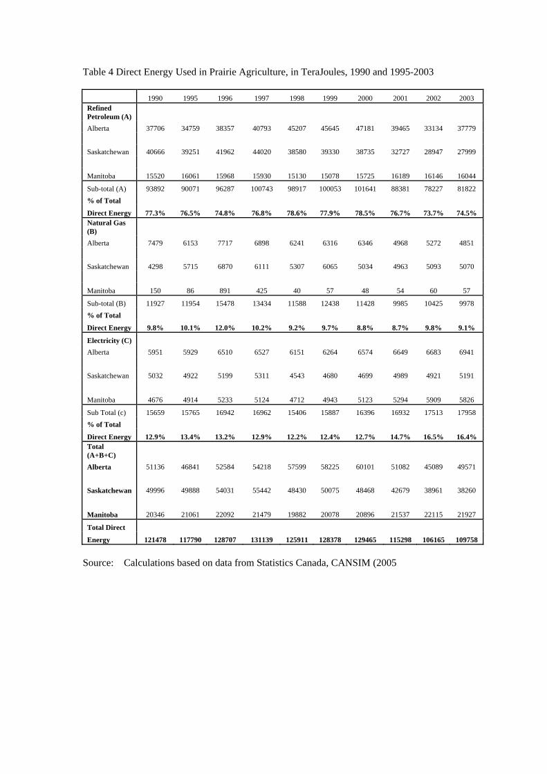
Table 4 Direct Energy Used in Prairie Agriculture, in TeraJoules, 1990 and 1995-2003

1990 1995 1996 1997 1998 1999 2000 2001 2002 2003 Refined Petroleum (A) Alberta 37706 34759 38357 40793 45207 45645 47181 39465 33134 37779 Saskatchewan 40666 39251 41962 44020 38580 39330 38735 32727 28947 27999

Manitoba 15520 16061 15968 15930 15130 15078 15725 16189 16146 16044

Sub-total (A) 93892 90071 96287 100743 98917 100053 101641 88381 78227 81822% of Total

Direct Energy 77.3% 76.5% 74.8% 76.8% 78.6% 77.9% 78.5% 76.7% 73.7% 74.5%Natural Gas (B) Alberta 7479 6153 7717 6898 6241 6316 6346 4968 5272 4851 Saskatchewan 4298 5715 6870 6111 5307 6065 5034 4963 5093 5070

Manitoba 150 86 891 425 40 57 48 54 60 57

Sub-total (B) 11927 11954 15478 13434 11588 12438 11428 9985 10425 9978 % of Total

Direct Energy 9.8% 10.1% 12.0% 10.2% 9.2% 9.7% 8.8% 8.7% 9.8% 9.1%

Electricity (C) Alberta 5951 5929 6510 6527 6151 6264 6574 6649 6683 6941 Saskatchewan 5032 4922 5199 5311 4543 4680 4699 4989 4921 5191

Manitoba 4676 4914 5233 5124 4712 4943 5123 5294 5909 5826

Sub Total (c) 15659 15765 16942 16962 15406 15887 16396 16932 17513 17958% of Total

Direct Energy 12.9% 13.4% 13.2% 12.9% 12.2% 12.4% 12.7% 14.7% 16.5% 16.4%Total (A+B+C) Alberta 51136 46841 52584 54218 57599 58225 60101 51082 45089 49571 Saskatchewan 49996 49888 54031 55442 48430 50075 48468 42679 38961 38260

Manitoba 20346 21061 22092 21479 19882 20078 20896 21537 22115 21927

Total Direct

Energy 121478 117790 128707 131139 125911 128378 129465 115298 106165 109758 Source: Calculations based on data from Statistics Canada, CANSIM (2005

80%Petrol

10%N Gas

10%Electricity

2000 77%Petrol

12%N Gas

12%Electricity

2001

74%Petrol

13%N Gas

13%Electricity

2002 73%Petrol

13%N Gas

14%Electricity

2003

Figure 1 Percentage share of natural gas, refined petroleum, and electricity in Saskatchewan agriculture, 2000-03

75%Petrol

0%N Gas

25%Electricity

2000 75%Petrol

0%N Gas

25%Electricity

2001

73%Petrol

0%N Gas

27%Electricity

2002 73%Petrol

0%N Gas

27%Electricity

2003

Figure 2 Percentage share of natural gas, refined petroleum, and electricity in Manitoba agriculture, 2000-03

79%Petrol

11%N Gas

11%Electricity

2000 77%Petrol

10%N Gas

13%Electricity

2001

73%Petrol

12%N Gas

15%Electricity

2002 76%Petrol

10%N Gas

14%Electricity

2003

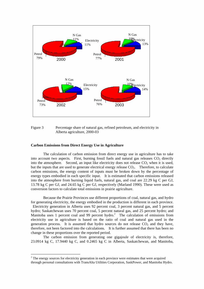
Figure 3 Percentage share of natural gas, refined petroleum, and electricity in Alberta agriculture, 2000-03 Carbon Emissions from Direct Energy Use in Agriculture The calculation of carbon emission from direct energy use in agriculture has to take into account two aspects. First, burning fossil fuels and natural gas releases CO2 directly into the atmosphere. Second, an input like electricity does not release CO2 when it is used, but the inputs that are used to generate electrical energy release CO2. Therefore, to calculate carbon emissions, the energy content of inputs must be broken down by the percentage of energy types embodied in each specific input. It is estimated that carbon emissions released into the atmosphere from burning liquid fuels, natural gas, and coal are 22.29 kg C per GJ, 13.78 kg C per GJ, and 24.65 kg C per GJ, respectively (Marland 1990). These were used as conversion factors to calculate total emissions in prairie agriculture. Because the Prairie Provinces use different proportions of coal, natural gas, and hydro for generating electricity, the energy embodied in the production is different in each province. Electricity generation in Alberta uses 92 percent coal, 3 percent natural gas, and 5 percent hydro; Saskatchewan uses 70 percent coal, 5 percent natural gas, and 25 percent hydro; and Manitoba uses 1 percent coal and 99 percent hydro.2 The calculation of emissions from electricity use in agriculture is based on the ratio of coal and natural gas used in the generation process. It is assumed that hydro sources do not release CO2 and they have, therefore, not been factored into the calculations. It is further assumed that there has been no change in these proportions over the reported period. The carbon emission from generating one gigajoule of electricity is, therefore, 23.0914 kg C, 17.9440 kg C, and 0.2465 kg C in Alberta, Saskatchewan, and Manitoba,

2 The energy sources for electricity generation in each province were estimates that were acquired through personal consultations with TransAlta Utilities Corporation, SaskPower, and Manitoba Hydro.

respectively. These per unit emissions were then multiplied by the total electrical energy used in agriculture to arrive at the CO2 emissions from farm electricity use. Table 5 summarizes the results of the estimated CO2 emissions from the direct energy use in agriculture. Refined petroleum is the greatest contributor to total CO2 emissions (76 percent). The use of natural gas has remained constant during the 1995 to 2003 and so has its contribution to total emissions (about 6%), whereas electrical energy use constitutes about 18 percent of total CO2 from direct energy use. Indirect Energy Use Indirect energy refers to the energy content of farm inputs, such as fertilizers, herbicides, farm buildings, and machinery. It is estimated that indirect energy accounts for approximately 60 percent of the total energy used in agricultural production in North America (Fluck 1992). In this report, the term "indirect energy" is used narrowly to include only fertilizers and farm chemicals. There are two reasons for this: first, estimating the energy content of farm machinery and buildings is very complicated, and second, the energy content of these inputs, like sunk costs, does not vary with production decisions. Fertilizers and herbicides are the most commonly used indirect energy inputs. The energy content of these inputs varies by the type of fertilizers and herbicides. The energy invested in producing, storing, and transporting fertilizers is assumed to be 60,700 KJ per kilogram of nitrogen, 12,560 KJ per kilogram of phosphate, and 6,700 KJ per kilogram of potash. The breakdown of energy in nitrogen fertilizer is 90 percent natural gas, 5.2 percent liquid fuels, and 4.8 percent electricity. The energy embodied in phosphate is 47.4 percent electricity, 26.7 percent liquid fuel, and 25.9 percent natural gas. Potash contains 42.1 percent electricity, 31.3 percent liquid fuel, and 26.7 percent natural gas (Pimentel 1980; and Lockeretz 1980).

Table 5 CO2 Emissions from Direct Energy Use, by Province, for 1990 and 1995-03 (tonnes of C)

1990 1995 1996 1997 1998 1999 2000 2001 2002 2003 Refined Petroleum (A) Alberta 840467 774778 854978 909276 1007664 1017427 1051664 879675 738557 842094 Saskatchewan 906445 874905 935333 981206 38602 876666 38757 729485 645229 624098

Manitoba 345941 358000 355927 355080 337248 336089 350510 360853 359894 357621

Sub-total (A) 2092853 2007683 2146237 2245561 1383514 2230181 1440932 1970012 1743680 1823812% of Total Direct Energy 79% 78% 77% 79% 70% 80% 72% 78% 75% 76% Natural Gas (B) Alberta 103061 84788 106340 95054 86001 87034 87448 68459 72648 66847 Saskatchewan 59226 78753 94669 84210 73130 83576 69369 68390 70182 69865

Manitoba 2067 1185 12278 5857 551 785 661 744 827 785

Sub-total (B) 164354 164726 213287 185121 159683 171396 157478 137593 143657 137497 % of Total Direct Energy 6% 6% 8% 6% 8% 6% 8% 5% 6% 6%

Electricity (C) Alberta 146692 146150 160472 160891 151622 154408 162049 163898 164736 171096 Saskatchewan 124039 121327 128155 130916 164250 115362 115830 122979 121303 127958

Manitoba 115263 121130 128993 126307 116151 121845 126282 130497 145657 143611

Sub Total (C) 385994 388607 417620 418113 432023 391615 404161 417374 431695 442665% of Total Direct Energy 15% 15% 15% 15% 22% 14% 20% 17% 19% 18% Total (A+B+C) Alberta 1090220 1005716 1121789 1165221 1245287 1258869 1301161 1112032 975941 1080036 Saskatchewan 1089710 1074985 1158157 1196332 275983 1075603 223956 920854 836713 821920

Manitoba 463271 480315 497198 487243 453950 458719 477454 492094 506378 502017Total Direct Energy 2643201 2561016 2777144 2848795 1975220 2793192 2002571 2524980 2319032 2403974

Source: Estimated Carbon Emissions from Indirect Energy Use in Agriculture Fertilizers, herbicides, and pesticides are used primarily for agricultural purposes. Like electrical energy, the use of these inputs does not release carbon directly but the inputs embodied in the manufacturing process contribute to CO2 emissions. CO2 emissions from fertilizer and herbicide use are based on the study by Yilidirim and Manaloor (1995). Nitrogen is the dominant source of CO2 emissions among the three fertilizers, with almost 90 percent of the total fertilizer energy derived from nitrogen and 90 percent of the total CO2 from fertilizer use associated with nitrogenous fertilizers.

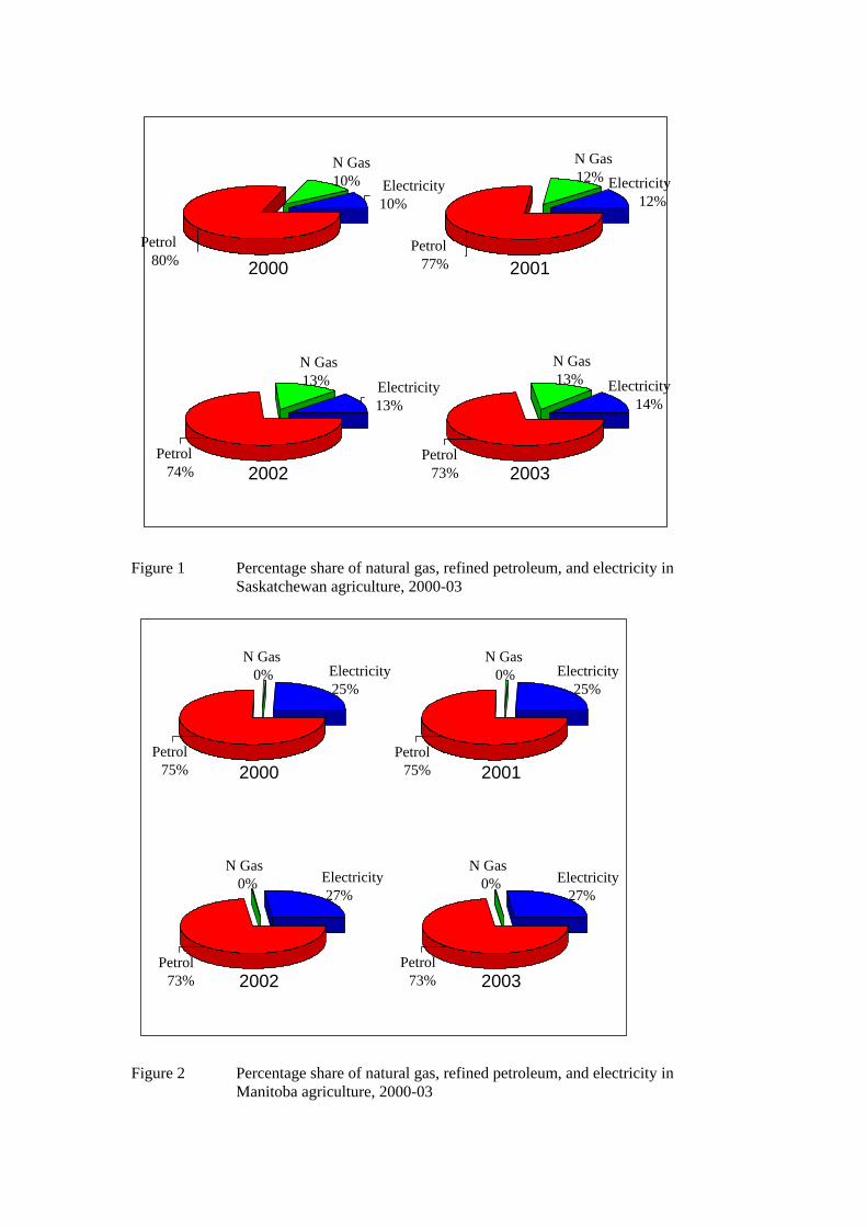
Figure 2.4 Total CO2 emissions from different energy inputs used in agriculture, 2000-03. Figure 4 shows the shares of CO2 emissions from different energy sources. The contribution of refined petroleum products to the total CO2 emission from agriculture varies from 48% to 55 % for the period 2000-03.

48%Ref.

Petroleum

N Gas13%

Total CO2 (2000) 3, 028, 614 tonnes Total CO2 (2001) 3, 551, 023 tonnes

Electricity2%Herbicides

31%Fertilizer

55%Ref.

Petroleum

4%N Gas 12%

Electricity2%

Herbicides

27%Fertilizer

Total CO2 (2002) 3, 345, 075 tonnes Total CO2 (2003) 3, 430, 017 tonnes

Empirical Analysis3

Conceptual Model The theoretical model that was used to investigate the determinants of energy demand in agriculture is a dual cost function. A dual cost function represents the minimum cost of producing a given level of output at a given set of input prices. Besides providing a solution to the multiple-output firms input decisions, this approach has several other advantages: (1) Economic theory establishes that the producer's decisions on all output supplies and input demands are interrelated by their common dependence upon the production possibilities frontier and the producer's objective function. Duality theory incorporates the behavioural hypothesis and the interrelations in production decisions to the estimation equations. (2) Dual cost functions are homogeneous of degree one in prices, regardless of the homogeneity properties of the underlying production function. Therefore, it does away with the necessity of imposing homogeneity conditions on the production process to arrive at estimation equations.

3 This section is taken from earlier study by Yildirim and Manaloor (1995)

52%Ref.

Petroleum

N Gas13%Electricity 2%

Herbicides

28%Fertilizer

53%PetroleumRef.

4%N Gas 13%

Electricity 2%Herbicides

28%Fertilizer

(3) Dual cost functions have prices as independent variables, which are exogenous to producers, rather than input quantities, which are choice variables. A dual cost function could be derived from a constrained cost minimization problem as follows:

( )[ ]Min L Min wj X jj

nq q X XnX j

s',....,=

=∑ + −

11λ (1)

where, Xj = Factors of production, j = 1, ....., n , wj = Input prices, j = 1, ......, n., q = q (X1, ....., Xn), production function. Solution to (1) yields the n constant-output factor demands , j = 1, ......, n.,

(2) ( )X X w wj q j q n/

*/

* ,....., ,= 1 q

where X*j/q refers to the demand for input j conditional on output level q. Substituting (2) into

( ) provides an expression for the minimum level of cost, Cw Xjj j∑ *, in terms of input prices

and output level: C*= C* (w1 , ....., wn , q). (3) Given that the production function in (1) is continuous and quasi-concave, to be interpreted as representing a theoretically valid output-constrained minimization of cost, any dual cost function derived from a direct objective function (1) must satisfy the following regularity conditions: (a) continuous with respect to input prices; (b) linearly homogeneous in input prices; (c) non decreasing in input prices; and, (d) concave in input prices. Once a dual cost function is specified so as to meet all regularity conditions, the system of input demand equations could be derived by applying Shepard's Lemma. The partial derivative of the dual cost function with respect to the jth input price yields the constant-output input demand function for input j: δ C*/ δ wj = ( )X X w wj q j q n/

*/

* ,....., ,= 1 q , for j=1, ... , n.

(4) The properties of the constant-output input demand function are as follows: (a) continuous with respect to input prices; (b) the slope of an input demand function with respect to own price, hence, the own-

price elasticity, is nonpositive (C* is concave in input prices); (c) homogeneous of degree zero in prices (C* is homogeneous of degree one in

input prices); and, (d) symmetric in input prices, which is also known as the integrability condition,

that is, (δ 2 C*/ δ wj δ wi = Cδ 2 */ δ wi δ wj, and, hence, δ Xj

* /δ wi = δ Xi*

/δ wj ).

Functional Form of Cost Functions Functional forms that have been utilized in past empirical analysis include the Cobb-Douglas, the Constant Elasticity of Substitution(CES), the Generalized Leontief, and the Translog. The Cobb-Douglas cost function corresponds to a Cobb-Douglas production function, and choosing this functional form automatically assumes a specific production technology. Unfortunately, the Cobb-Douglas form imposes serious and perhaps unrealistic restrictions on the production process. The CES cost function corresponds to a CES production function, and choosing this functional form also automatically assumes a certain production technology. While it is not as restrictive as the Cobb-Douglas form, the CES form still imposes the elasticities between each pair of inputs to be the same. There are two concerns in the choice of functional form: it should be simple enough to estimate, and it should not impose too many a priori restrictions on economic parameters. Two functional forms--the Generalized Leontief Cost Function and the Translog Cost Function--provide more flexibility. In this analysis, the following Translog Cost Function was utilized for empirical estimations: ln C(w,q) = ao + aq ln q + Σj aj ln wj + (1/2) Σj Σk bjk ln wj.ln wk

+ Σj bjq ln wj. ln q + Σj bjt ln wj ln t.

(5)

Then, applying Shepard's Lemma to (5) yields the following input share equations: δ ln C/ δ ln wj = (δC/C)/ (δwj/wj) = (δC/δwj).(wj/C)= (Xj w))/C = Sj, Hence, Sj = aj + Σk bkj. ln wk + bjq ln q + bjt ln t, for j= 1, 2, . . . ,n. (6) Regularity conditions in this case translate into the following: homogeneity of degree one in prices implies that Σj aj = 1, Σj bjk = 0, and Σkbjk = 0. The equality of second order cross-derivatives implies the symmetry constraint, bjk= bkj, and concavity implies that the matrix of second derivatives of the cost function with respect to input prices is negative semi-definite or the matrix of partial elasticities of substitution is negative semi-definite. Elasticities The estimated price coefficients of this model have no economic interpretation on their own. However, they are used together with predicted input shares to calculate the elasticities of substitution (σ) and price elasticities of input demands (η). The formulas used in these equations are given below: σjk = [bjk/(Sj Sk)]+ 1 for all j, k; σjj = [(bjj+ Sj

2 - Sj)/ Sj2] for all j;

ηjj = σjj Sj for all j; ηjk = σjk Sj for all j, k.

Data This analysis requires data on farm input expenditures, cost of production, total farm production, and input prices. Data on aggregate output and inputs were used to estimate the input share equations. As a measure of total production, an aggregate output index was used. Output indices for the three provinces were obtained from Agriculture and Agri-Food Canada. A regional aggregate index for the Prairies was computed using total cash receipts as weights. Data on expenditures were obtained from Statistics Canada, CANSIM data base. Expenditures on inputs were grouped into six categories: direct energy, indirect energy, machinery, labour, land and buildings, and miscellaneous inputs. The direct energy category includes the farm portion of electricity and fuel expenditures. The indirect energy includes expenditures on fertilizers, lime, and pesticides. Expenditures on machinery repair and depreciation were used to reflect expenditures on machinery services. Similarly, depreciation on buildings, cash and share rent, property taxes, and repairs to buildings and fences were used to represent annual expenditures on the services of land and buildings. Labour expenditures include the wages of the farm operator and family labour, and wages paid to hired labour. Data on wages and the number of hours worked by the three categories of labour were obtained from the Policy Branch of Agriculture and Agri-Food Canada. The miscellaneous inputs category includes expenditures on seed, irrigation, twine, wire and containers, custom work, and expenses on livestock. A weighted aggregate price index was calculated for each input group that had an available provincial price index. Data on price indices were obtained from the CANSIM data base of Statistics Canada. The weights used are the respective provincial expenditures. In cases where provincial price indices were not reported, the Western Canadian price index was used. Results Elasticities of Substitution The estimates of Allen Partial Elasticities of Substitution (AES) are reported in Table 6. AES measures the rate at which one input could substitute for another as the relative prices of these inputs change. Positive values indicate that the respective inputs are substitutes for each other. That is, as the price of one input relative to another increases the use of more expensive input vis-à-vis the other declines, while producing the same level of output. Negative signs imply a complementary relationship, that is, the use of two inputs in question change in the same direction in response to changes in relative prices. Table 6 Estimated Allen Partial Elasticities of Substitution

Direct Energy

Indirect Energy

Machinery Land & Bldgs

Miscellaneous Inputs

Labour -0.149 0.590 0.169 0.475 1.536

Direct Energy 2.932 0.679 0.508 -0.231

Indirect Energy 3.859 3.298 -2.738

Machinery 1.806 2.355

Land & Bldgs -1.582

Source: Estimated The estimated elasticity of substitution between labour and direct energy input pair is -0.149. This indicates that in response to a 1 percent increase in the wage rate/direct energy price ratio, the use of direct energy vis-à-vis labour will decrease by 0.14 percent. That is, labour and direct energy are complementary inputs. The elasticity of substitution for labour and indirect energy input pair is 0.59, which shows that a 1 percent increase in the labour/indirect energy price ratio will result in a 0.59 percent increase in the use of indirect energy vis-à-vis the quantity of labour. In other words, as labour becomes relatively more expensive, indirect energy inputs will substitute for labour in the production process. Our results also show that machinery services, land services, and miscellaneous inputs are substitutes for labour, with labour and miscellaneous inputs pair showing the largest substitution possibility (1.53). Direct energy and indirect energy inputs are substitutes in production, with the estimated elasticity of substitution being 2.93. This indicates that a 1 percent increase in the direct/indirect energy price ratio will result in indirect energy substituting for direct energy, and indirect energy/direct energy input use ratio will increase by 2.93 percent. This result is not surprising, considering that in certain activities, such as weed control and mechanical and chemical technologies, direct and indirect energy inputs substitute for each other as relative prices change. A good example of this is the recent increase in the area seeded with reduced tillage technology. This technology substitutes chemical weed control for mechanical weed control, so that while it saves labour and machinery time and direct energy inputs, it uses more herbicides, and hence indirect energy than the conventional tillage. This result is very crucial in assessing the impacts of direct energy-saving production techniques on CO2 emissions since indirect energy use will increase in response to a decline in direct energy use. The estimates also reveal that the elasticity of substitution for direct energy and machinery pair is 0.67, and for direct energy and land pair is 0.588, suggesting that their substitutability is not as high as between direct energy and indirect energy. Direct energy and miscellaneous inputs pair are complementary inputs with an estimated elasticity of (-0.23). This is an expected result as the increased use of miscellaneous inputs, such as seed, would result in an increased use of machinery and, hence, of direct energy. The elasticity of substitution between indirect energy and machinery services (3.8) is the highest among all input pairs and is consistent with the high elasticity of substitution between direct and indirect energy inputs. That is, a decrease in the price of herbicides relative to that of machinery services makes chemical weed control profitable and results in decreased use of both machinery and direct energy. Indirect energy and land pairs are also substitutes (3.298), indicating that as fertilizer prices come down, fertilizers would substitute for land services in production. This implies a switch from extensive to intensive production techniques. Indirect energy and miscellaneous inputs have the highest elasticity of substitution, -2.738, among all input pairs considered, indicating that a 1 percent increase in the indirect energy/miscellaneous inputs price ratio would result in a 2.738 percent decrease in the miscellaneous inputs/indirect energy use ratio. Similarly, machinery and land services, and machinery services and miscellaneous inputs are substitutes for each other. Land and miscellaneous inputs are complements in production. Own- and Cross-Price Elasticities Table 7 shows the own- and cross-price elasticities of demand for inputs employed in prairie agriculture. Own-price elasticity measures the responsiveness of the demand for an input to a change in its price. Own-price elasticity of demand is always negative, indicating that as the price of an input increases (decreases), the demand for this input decreases (increases). Cross-price elasticity measures the responsiveness of the demand for an input to the changes in the price of some other input. The sign of the cross-price elasticity depends on the interrelationship amongst input pairs. It is positive for those input pairs that are substitutes in production, and negative for those that are complements.

All of the estimated own-price elasticities, which are reported as the diagonal elements of Table 7 have negative signs, as expected. The magnitude of each of these elasticities is less than one, with the exception of indirect energy input. This implies that the responsiveness of the demand for any particular input to a change in its own price is rather low, especially for labour and direct energy inputs. The estimated own-price elasticity of direct energy input is (-0.3147). That is, in response to a 1 percent increase in energy price, agricultural energy use would decrease by only 0.31 percent. The estimated cross-price elasticities with respect to direct energy price are also very small, indicating that a change in the direct energy price would have very little impact on the demand for other inputs. They also indicate that labour and miscellaneous inputs category are complementary inputs to direct energy, while indirect energy, machinery services, and the services of land and buildings are substitutes for direct energy. The cross-price elasticity of labour with respect to direct energy price is (-0.1154), which suggests that if energy prices increase by 1 percent the demand for labour would decrease by 0.1154 percent. Similarly, the cross price elasticity of miscellaneous inputs with respect to direct energy price (-0.0179) indicates a very small decline in the use of these inputs as energy prices increase. A 1 percent increase in direct energy price will result in 0.23, 0.05, and 0.034 percent increase in the demand for indirect energy, machinery, and land inputs, respectively. The cross-price elasticity of energy demand with respect to other input prices is also very small, indicating that energy demand would change very little in response to changes in the prices of these inputs. Table 7 Estimated Own- and Cross-Price Elasticities of Input Demands in the Prairies.

Prices of Quantity

Labour Direct Energy

Indirect Energy

Machinery Land & Bldgs

Misc. Inputs

Labour -0.2706 -0.1154 0.0475 0.0309 0.0434 0.1602

Direct Energy -0.0688 -0.3147 0.2366 0.1245 0.0464 -0.0242

Indirect

Energy

0.2727 0.2274 -1.2243 0.7081 0.3017 -0.2856

Machinery 0.0779 0.0526 0.3114 -0.8530 0.1652 0.2457

Land & Bldgs 0.2195 0.0339 0.2661 0.3313 -0.6913 -0.1651

Miscellaneous Inputs

0.7101 -0.0179 -0.2208 0.4321 -0.1447 -0.7587

Source: Estimated The demand for indirect energy, on the other hand, is quite responsive to a change in its own price: a 1 percent increase in the price of indirect energy input leads to a 1.22 percent decrease in indirect energy use. The estimated cross-price elasticities are again rather small, and the signs of these elasticities indicate that miscellaneous inputs and indirect energy are complements in production, while all other input categories are substitutes for indirect energy. For example, if indirect energy price goes up by 1 percent the demand for miscellaneous inputs would fall down by 0.22 percent, while the same price change would result in 0.047 percent increase in the demand for labour, 0.236 percent increase in direct energy demand, 0.3114 percent increase in the demand for machinery services, and 0.266 percent increase in the demand for the services of land and buildings. The estimated cross-price elasticities of demand for indirect energy with respect to other input prices, which are all less than one. This indicates that indirect energy use would change very little in response to changes in other input prices.

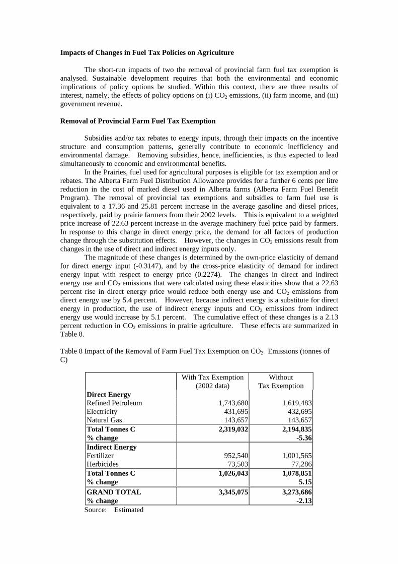
Impacts of Changes in Fuel Tax Policies on Agriculture The short-run impacts of two the removal of provincial farm fuel tax exemption is analysed. Sustainable development requires that both the environmental and economic implications of policy options be studied. Within this context, there are three results of interest, namely, the effects of policy options on (i) CO2 emissions, (ii) farm income, and (iii) government revenue. Removal of Provincial Farm Fuel Tax Exemption Subsidies and/or tax rebates to energy inputs, through their impacts on the incentive structure and consumption patterns, generally contribute to economic inefficiency and environmental damage. Removing subsidies, hence, inefficiencies, is thus expected to lead simultaneously to economic and environmental benefits. In the Prairies, fuel used for agricultural purposes is eligible for tax exemption and or rebates. The Alberta Farm Fuel Distribution Allowance provides for a further 6 cents per litre reduction in the cost of marked diesel used in Alberta farms (Alberta Farm Fuel Benefit Program). The removal of provincial tax exemptions and subsidies to farm fuel use is equivalent to a 17.36 and 25.81 percent increase in the average gasoline and diesel prices, respectively, paid by prairie farmers from their 2002 levels. This is equivalent to a weighted price increase of 22.63 percent increase in the average machinery fuel price paid by farmers. In response to this change in direct energy price, the demand for all factors of production change through the substitution effects. However, the changes in CO2 emissions result from changes in the use of direct and indirect energy inputs only. The magnitude of these changes is determined by the own-price elasticity of demand for direct energy input (-0.3147), and by the cross-price elasticity of demand for indirect energy input with respect to energy price (0.2274). The changes in direct and indirect energy use and CO2 emissions that were calculated using these elasticities show that a 22.63 percent rise in direct energy price would reduce both energy use and CO2 emissions from direct energy use by 5.4 percent. However, because indirect energy is a substitute for direct energy in production, the use of indirect energy inputs and CO2 emissions from indirect energy use would increase by 5.1 percent. The cumulative effect of these changes is a 2.13 percent reduction in CO2 emissions in prairie agriculture. These effects are summarized in Table 8. Table 8 Impact of the Removal of Farm Fuel Tax Exemption on CO2 Emissions (tonnes of C)

With Tax Exemption (2002 data)

Without Tax Exemption

Direct Energy Refined Petroleum 1,743,680 1,619,483 Electricity 431,695 432,695 Natural Gas 143,657 143,657 Total Tonnes C 2,319,032 2,194,835 % change -5.36 Indirect Energy Fertilizer 952,540 1,001,565 Herbicides 73,503 77,286 Total Tonnes C 1,026,043 1,078,851 % change 5.15 GRAND TOTAL 3,345,075 3,273,686 % change -2.13

Source: Estimated

These calculations did not take into account substitution possibilities between petroleum products and electricity and natural gas, which are likely to be negligible, at least in the short run. The substitution of indirect energy for direct energy inputs, however, indirectly causes inter-fuel substitution. Whereas petroleum products constitute a large percentage of direct energy use in prairie agriculture, indirect energy inputs, such as fertilizers, mostly require natural gas in the production process. Therefore, substituting indirect energy for direct energy, by increasing natural gas use and reducing petroleum products’ consumption, inadvertently causes inter-fuel substitution. Another important aspect of the removal of provincial farm fuel tax rebate programs is its potential impact on farm expenditures and income. These changes result from changes in the quantity of fuel and other inputs used in the production process, and changes in farm fuel prices. As a result of the calculated 22.63 percent increase in farm fuel prices, the demand for inputs that are substitutes for direct energy input, namely, indirect energy, machinery, and land and buildings, would increase, and the demand for complementary inputs, namely, labour and miscellaneous inputs, would decrease. Once all factor substitutions are made, the cost of producing the same level of output is estimated to increase by 0.56 percent. Keeping the level of output and output prices constant, this translates into an equal amount of decline in net cash income. Consequently, net cash income in the prairies is estimated to decrease by 1.63 percent. Table 9 Economic Effects of the Removal of Provincial Farm Fuel Tax Exemptions (`000 $)

2002(1)After the Removal of Tax Exemption

Net Cash

Income Net Cash Income

Change inNet Cash Income

% Change in Net Cash

Income

Change in Tax

Revenue

Net Welfare Gains

Manitoba 1,055,700 1,039,293 -16,407 -1.55 +49,531 +33,123

Saskatchewan 1,501,300 1,473,314 -27,986 -1.86 +108,210 +80,224

Alberta 2,404,100 2,367,675 -36,425 -1.52 +111,369 +74,944

TOTAL 4,961,100 4,880,282 -80,818 -1.63 +269,110 +188,292

Source: Estimated. Note: (1) Statistics Canada, CANSIM. The removal of provincial tax rebate/exemption programs would result in a different rate of change in net cash income in each province because of the differences in input use across the provinces. The values reported in the “Change in Tax Revenue” column of Table 9 are estimates of the cost of these programs to provinces, which would have been collected as tax revenue if there were no farm fuel tax rebate programs. In each province, the estimated change in tax revenues exceeds the predicted decline in farm income, indicating net welfare gains from the policy change. In summary, the removal of provincial farm fuel tax exemption would (i) reduce CO2 emissions by 2.13 percent from 2002 levels, (ii) improve efficiency in resource allocation, and (iii) result in net economic gains. In other words, provincial governments could compensate farmers, in a non-distorting way, for the losses in farm income and society overall would still be better off.

The emission levels in 1990 from Western Canadian agriculture when compared to the 2002 levels show that approximately 6 percent reductions have been achieved. This could be because of the increase in direct energy prices and the changes in farming practices.

List of References

Agriculture and Agri-Food Canada. (2000). Reducing Greenhouse Gas Emissions from Canadian Agriculture. Options Report of the Agriculture and Agri-Food Climate Change. Ottawa.

Agriculture Canada, Policy Branch. December 1990 Market Commentary: Farm Inputs

and Finance. Ottawa: Agriculture Canada. Canada’s National Action Program on Climate Change, (1995). Document tabled for the

first meeting of the Conference of the Parties to the Framework Convention on Climate Change on behalf of all federal, provincial, and territorial Energy and Environment ministers in Canada. Ottawa.

Carraro, C., and D. Siniscalco. (1994). Environmental Policy Reconsidered: The Role of

Technological Innovation. European Economic Review 38: 545-54. Climate Change Task Group. (1994). Report on Options for Canada’s National Action

Program on Climate Change. Ottawa. Fluck, R. C., ed. (1992). Energy in Farm Production, Volume 6 of Energy in World

Agriculture. Elsevier. Karagiannis, G., and W.H. Furtan. (1990). Induced Innovation in Canadian Agriculture:

1926-87. Canadian Journal of Agricultural Economics 38: 1-21 Lockeretz, W. 1980. Energy Inputs for Nitrogen, Phosphorous, and Potash Fertilizers. In

Handbook of Energy Utilization in Agriculture, edited by D. Pimentel. Boca Raton, Florida: CRC Press.

Lopez, R.E., and Fu-Lai Tung. (1982). Energy and Non-Energy Input Substitution

Possibilities and Output Scale Effects in Canadian Agriculture. Canadian Journal of Agricultural Economics 30: 115-32.

Marland, G., and A.F. Turhollow. (1990). CO2 Emissions from Production and

Combustion of Fuel Ethanol from Corn. Oak Ridge, Tennessee: Oak Ridge National Laboratory. ORNL/TM-11180.

Olsen, K., P. Collas, P. Boilleau, D. Blain, C. Ha, L. Henderson, C. Liang, S. McKibbon and

L. Morel-a-l’Huissier. 2002. Canada’s Greenhouse Gas Inventory 1990-2000. Ottawa: Environment Canada.

Pimentel, D. (1980). Energy Inputs for the Production, Formulation, Packaging, and

Transport of Various Pesticides. In Handbook of Energy Utilization in Agriculture, edited by D. Pimentel, Boca Raton, Florida: CRC Press.

Saskatchewan Energy Conservation and Development Authority, May 1993. A Report on

Energy Use in Saskatchewan Agricultural and Residential Sectors. Saskatoon: SECDA. Publication No. G800-93-P-002.

Statistics Canada. 2005. CANSIM. Ottawa: Statistics Canada. Yildirim T. and V. Manaloor. (1995). Energy and Non-Energy Input Substitution in

Agriculture: A Case Study of the Prairie Provinces. CAEDAC: Report no. 4/95, University of Saskatchewan.

Yildirim T., V. Manaloor and R. White. (1995). The Impacts of Energy Taxes on CO2

Emissions and Farm Income in Prairie Agriculture, CAEDAC, Report no. 5/95, University of Saskatchewan.