THE IMPACTS OF CLIMATE CHANGE ON AGRICULTURAL …

Page | i

Economic Commission for Latin America and the Caribbean

Subregional Headquarters for the Caribbean

AN ASSESSMENT OF THE ECONOMIC IMPACT OF CLIMATE CHANGE ON THE AGRICULTURE SECTOR IN TRINIDAD AND

TOBAGO

__________

This document has been reproduced without formal editing

LIMITED LC/CAR/L.321 22 October 2011 ORIGINAL: ENGLISH

Page | i

Table of Contents

List of Tables ............................................................................................................................................... iii List of Figures .............................................................................................................................................. iv Executive Summary .................................................................................................................................... vii INTRODUCTION ........................................................................................................................................ 1

A. OBJECTIVES ...................................................................................................................................... 2 B. THE ECONOMY OF TRINIDAD AND TOBAGO ........................................................................... 2 C. TRINIDAD AND TOBAGO‘S AGRICULTURAL SECTOR PERFORMANCE ............................. 4 D. PHYSICAL AND SOCIO-ECONOMIC VULNERABILITIES OF THE CARIBBEAN ................ 11

1. Land Capability ............................................................................................................................... 11 II. CLIMATE CHANGE IMPACTS ON AGRICULTURE ...................................................................... 15 III. LITERATURE REVIEW ..................................................................................................................... 16

A. MODELS ........................................................................................................................................... 16 B. DATA ................................................................................................................................................. 21

1. Climate Data ................................................................................................................................... 21 2. Root Crop and Vegetable Data ....................................................................................................... 21 3. Cocoa .............................................................................................................................................. 22 4. Fisheries .......................................................................................................................................... 22

IV. METHODOLOGY ............................................................................................................................... 23 A. MODELS ........................................................................................................................................... 23 B. RESULTS AND FORECASTS ......................................................................................................... 24 1. Key Model Variables .......................................................................................................................... 24

2. Baseline Case .................................................................................................................................. 27 3. A2 and B2 Scenarios ....................................................................................................................... 29

C. AGGREGATE VALUE OF YIELD LOSS FOR ROOT CROPS, FISHERIES AND VEGETABLE PRODUCTION ....................................................................................................................................... 41 D. POTENTIAL LAND LOSS ............................................................................................................... 42

IV. ADAPTATION OPTIONS AND BENEFIT COST ANALYSES ....................................................... 45 VI. CONSIDERATIONS FOR MITIGATION OPTIONS IN TRINIDAD AND TOBAGO.................... 63

A. EMISSIONS....................................................................................................................................... 63 B. LAND LOSS DUE TO FOREST FIRES ........................................................................................... 64

Page | ii

C. CLIMATE CHANGE AND THE IMPLICATIONS FOR FOOD SECURITY ................................ 65 D. DATA NEEDS FOR FUTURE WORK ............................................................................................ 65

VII. CONCLUSIONS ................................................................................................................................. 66 REFERENCES ........................................................................................................................................... 68

Page | iii

List of Tables

Table 1: Real GDP Growth Rate of Trinidad and Tobago ............................................................................ 3 Table 2: Real GDP Growth Rate of Trinidad and Tobago ............................................................................ 4 Table 3: Agricultural and Forest Land Area (1000 Hectares) and Tractor Use, Selected Years .................. 6 Table 4: Key Components of Agricultural GDP ........................................................................................... 7 Table 5: Climate Change and Related Factors Relevant to Agricultural Production at the Global Scale .. 15 Table 6: Descriptive Statistics of Model Variables .................................................................................... 24 Table 7: Estimated Total Annual Value (Millions TT$) of Fish Landings for Trinidad from 2001-2008 . 28 Table 8: Historical and Projected Mean Monthly Temperature and Rainfall – Trinidad & Tobago for the A2 and B2 Scenarios ................................................................................................................................... 30 Table 9: Historical and Projected Mean Monthly Temperature – Trinidad & Tobago for the A2 and B2 Scenarios, by Season ................................................................................................................................... 30 Table 10: Historical and Projected Mean Monthly Rainfall – Trinidad & Tobago for the A2 and B2 Scenarios, by Season ................................................................................................................................... 31 Table 11: Model Estimates for Root Crop Yield (RC) ............................................................................... 31 Table 12: Breusch-Godfrey Serial Correlation LM Test for the Root Crops Model .................................. 32 Table 13: Results of Unit Root tests for logged model variables ............................................................... 32 Table 14: Inverse Roots of AR/MA Polynomial(s) for the Root Crops Model .......................................... 33 Table 15: Present Value of Root Crop Cumulative Losses Relative to the Baseline* (TT $mil) ............... 35 Table 16: SIC Values of ARMA Variations of the Basic Cocoa Model..................................................... 35 Table 17: Present Value of Cumulative Losses Relative to the Baseline (TT$mil) ................................... 37 Table 18: Model Estimates for Green Vegetables ...................................................................................... 37 Table 19: Breusch-Godfrey Serial Correlation LM Test for the Green Vegetables Model ........................ 38 Table 20: Results of Unit Root Tests for Logged Model Variables ........................................................... 38 Table 21: Inverse Roots of AR/MA Polynomial(s) for the Green Vegetables Model ................................ 39 Table 22: Present Value of Cumulative Vegetable Losses Relative to the Baseline (TT $mil) ................. 41 Table 23: Present Value of Cumulative Losses for Agricultural Yield Relative to the Baseline (TT $mil) .................................................................................................................................................................... 41 Table 24: Estimate of the Cumulative Cost of the Impact of Climate Change (in 2008 GDP* % of the Net Present Value) ............................................................................................................................................. 42 Table 25: Summary of the Present Value Costs and Benefits of the Highest-Ranked Proposed Adaptation Actions for Trinidad and Tobago (4% Discount Rate) ............................................................................... 47 Table 26: Breakdown of Food Storage Costs ............................................................................................. 60 Table 27: Greenhouse Installation Costs .................................................................................................... 62 Table 28: CO2 Emissions in 2006 ............................................................................................................... 63

Page | iv

Table 29: Number and Size of Fires in Trinidad and Tobago, 2005 - 2009 ............................................... 64 Table 30: Estimated Total Annual Landings (tonnes) by Fleet from the Marine Capture Fisheries of Trinidad & Tobago for 1996-2008 (Fisheries Division records). ............................................................... 74 Table 31: Root Crop and Vegetable Climate Ranges ................................................................................. 75 Table 32: Cocoa Model .............................................................................................................................. 76 Table 33: Omitted Variables Tests.............................................................................................................. 76 Table 34: Potential Risks and Adaptation Options ..................................................................................... 77

List of Figures Figure 1: Real GDP Growth Rate of Trinidad and Tobago (%) ................................................................... 3 Figure 2: Real GDP (at Factor Cost) of Trinidad and Tobago ...................................................................... 3 Figure 3: Inflation Rate in Trinidad and Tobago (%) ................................................................................... 4 Figure 4: Agricultural GDP and Associated Growth Rate for Trinidad and Tobago ................................... 5 Figure 5: Percentage Contribution to GDP by Sector in Trinidad and Tobago, 1997 .................................. 5 Figure 6: Percentage Contribution to GDP by Sector in Trinidad and Tobago, 2009 .................................. 6 Figure 7: Key Commodities – 2008 (Contribution to Domestic Agriculture) .............................................. 7 Figure 8: Holders in Trinidad and Tobago by Type of Agricultural Activity ............................................... 8 Figure 9: Distribution of Holders by Type of Agricultural Activity and Parishes in Trinidad ..................... 9 Figure 10: Distribution of Holders by Type of Agricultural Activity and Parishes in Tobago .................... 9 Figure 11: Distribution of Holders by Type of Agricultural Production (a) in Trinidad and (b)Tobago.... 10 Figure 12: Distribution of Holders by Size in Trinidad and Tobago, 2004 ................................................ 10 Figure 13: Distribution of Holders by Age Group in Trinidad and Tobago, 2004 ..................................... 11 Figure 14: Land Utilized for Agriculture in Trinidad ................................................................................. 12 Figure 16: Historical Mean Monthly Rainfall – Trinidad and Tobago (1970-2008) (mm) ........................ 25

Figure 17: Historical Mean Monthly Temperature – Trinidad and Tobago (1970-2008) ( C) ................... 25 Figure 18: Monthly Values of Model Variables (in levels) from 1995-2008 ............................................. 26 Figure 19: Monthly Trips, 1996 – 2008 (a), and Nominal and Real Fish Prices (b) .................................. 28 Figure 20: Historical and Projected Mean Monthly Rainfall – Trinidad & Tobago for the A2 and B2 Scenarios ..................................................................................................................................................... 29 Figure 21: Historical and Projected Mean Monthly Temperature – Trinidad & Tobago for the A2 and B2 Scenarios ..................................................................................................................................................... 30 Figure 22: Forecasted Harvest of Root Crops Under the Business as Usual Scenario, 1996-2050 (‗000 kg) .................................................................................................................................................................... 33 Figure 23: Projections for Root Crop Harvests under the BAU, A2 and B2 Scenarios (‗000 kg) .............. 34 Figure 24: Cumulative Values of Root Crop Production ............................................................................ 34 Figure 25: Predicted Changes in Global Catch Potentials .......................................................................... 36

Page | v

Figure 26: Forecasted Green Vegetable Harvests Under the Business as Usual Scenario, 1996-2050 (‗000 kg) ............................................................................................................................................................... 39 Figure 27: Projections for the Value of Vegetable Yield under the BAU, A2 and B2 Scenarios (‗000 TT$) .................................................................................................................................................................... 40 Figure 28: Cumulative Values of Root Crop Production ............................................................................ 40 Figure 29: Projected Agricultural Land and Wetlands under a 0.255 m Sea Level Rise with 0.5m High Tide (Shown as Pink Labeled Areas) .......................................................................................................... 43 Figure 30: Projected Land under a 0.255 m Sea Level Rise and High Rainfall Intensity Event ................ 44 Figure 31: Agricultural Land Zones Adjacent to the Caroni Swamp ......................................................... 44 Figure 32: Per-Capita CO2 Emissions for Selected Caribbean Countries, 2006 ......................................... 63

Page | vi

Acknowledgement

The Economic Commission for Latin America and the Caribbean (ECLAC) Subregional Headquarters for the Caribbean, wishes to acknowledge the assistance of Sharon Hutchinson, consultant, in the preparation

of this report.

Page | vii

Executive Summary

The economic impact of climate change on root crop, fisheries and vegetable production for Trinidad and Tobago under the A2 and B2 scenarios were modeled, relative to a baseline ―no climate change‖ case, where the mean temperature and rainfall for a base period of 1980 – 2000 was assumed for the years up to 2050. Production functions were used, using ARMA specifications to correct for serial autocorrelation. For the A2 scenarios, rainfall is expected to fall by approximately 10% relative to the baseline case in the 2020s, but is expected to rise thereafter, until by the 2040s rainfall rises slightly above the mean for the baseline case. For the B2 scenario, rainfall rose slightly above the mean for the baseline case in the current decade, but falls steadily thereafter to approximately 15% by the 2040s. Over the same period, temperature is expected to increase by 1.34 C and 1.37 C under A2 and B2 respectively.

It is expected that any further increase in rainfall should have a deleterious effect on root crop production as a whole, since the above mentioned crops represent the majority of the root crops included in the study. Further expected increases in temperature will result in the ambient temperature being very close to the optimal end of the range for most of these crops. By 2050, the value of yield cumulative losses (2008$) for root crops is expected to be approximately 248.8 million USD under the A2 scenario and approximately 239.4 million USD under the B2 scenario.

Relative to the 2005 catch for fish, there will be a decrease in catch potential of 10 - 20% by 2050 relative to 2005 catch potentials, other things remaining constant. By 2050 under the A2 and B2 scenarios, losses in real terms were estimated to be 160.2 million USD and 80.1 million USD respectively, at a 1% discount rate.

For vegetables, the mean rainfall exceeds the optimal rainfall range for sweet peppers, hot peppers and melongene. However, while the optimal rainfall level for tomatoes is 3000mm/yr, other vegetables such as sweet peppers, hot peppers and ochroes have very low rainfall requirements (as low as 300 mm/yr). Therefore it is expected that any further decrease in rainfall should have a mixed effect on individual vegetable production. It is expected that any further increase in temperature should have a mixed effect on individual vegetable production, though model results indicated that as a group, an increase in temperature should have a positive impact on vegetable production. By 2050, the value of yield cumulative gains (2008$) for vegetables is expected to be approximately 54.9 million USD under the A2 scenario and approximately 49.1 million USD under the B2 scenario, given a 1% discount rate.

For root crops, fisheries and vegetables combined, the cumulative loss under A2 is calculated as approximately 352.8 million USD and approximately 270.8 million USD under B2 by 2050. This is equivalent to 1.37% and 1.05% of the 2008 GDP under the A2 and B2 scenarios respectively by 2050.

Sea Level Rise (SLR) by 2050 is estimated to be 0.255 m under A2 and 0.215 m under B2. GIS estimation indicated that for a 0.255 m sea level rise, combined with a 0.5 m high tide, there would be no permanent inundation of agricultural land in Trinidad. The total inundation area is 1.18 km2. This occurs only in the Caroni Watershed, on the western coast of Trinidad, and the areas are outside the Caroni Swamp. Even with an additional rise of 0.5 m to simulate a high rainfall event, the estimated inundated area is 4.67 km2, but with no permanent inundation, though likely to be subject to flooding.

Based on eleven (11) evaluation criteria, the top potential adaptation options were identified: 1. Use of water saving irrigation systems and water management systems e.g. drip irrigation; 2. Mainstream climate change issues into agricultural management; 3. Repair/maintain existing dams;

Page | viii

4. Alter crop calendar for short-term crops; 5. Adopt improved technologies for soil conservation; 6. Establish systems of food storage; 7. Promote water conservation – install on-farm water harvesting off roof tops; 8. Design and implement holistic water management plans for all competing uses; 9. Build on- farm water storage (ponds and tanks); 10. Agricultural drainage; and 11. Installation of greenhouses.

The most attractive adaptation options, based on the Benefit-Cost Ratio are: (1) Build on- farm water

storage such as ponds and tanks (2) Mainstreaming climate change issues into agricultural management and (3) Water Harvesting. However, the options with the highest net benefits are, (in order of priority): (1) Build on- farm water storage such as ponds and tanks, (2) Mainstreaming climate change issues into agricultural management and (3) Use of drip irrigation.

Based on the area burnt in Trinidad and Tobago between 2005 and 2009, the average annual loss due

to fires is 1717.3 ha. At US$17.41 per carbon credit, this implies that for the total land lost to forest fires on average each year, the opportunity cost of carbon credit revenue is 74.3 million USD. If a teak reforestation programme is undertaken in Trinidad and Tobago, the net benefit of reforestation under a carbon credit programme would be 69 million USD cumulatively to 2050.

Page | 1

I. INTRODUCTION

There is increasing evidence that anthropogenic activities are already impacting negatively on the world‘s climate. As a result, all countries are now seeking to determine the likely impact of joint and interrelated actions on the global commons, and more importantly, to find ways to reduce the potential negative impacts, while preparing local communities for change in order to cope with and/or even benefit from the projected changes. Fortunately, many countries are already making changes to reduce their emissions of greenhouse gases (GHG) in some sectors, through policy and legislative changes. However, other countries are vigorously trying to maintain their status quo, or are achieving very little changes in their contribution to climate change, as the final output relies heavily on individuals and firms making changes to their economic behavior, which may come at a personal cost, even though the aggregate benefit to society may vastly outweigh the sum of the individual costs.

In order to determine the impact of climate change on the agricultural sector in the Caribbean, a baseline period was first established. The IPCC‘s Special Report on Emissions Scenarios (SRES) A21 and B22 scenarios were then used as the projected future climate for the Caribbean (IPCC, 2000a). Using Atmosphere-Ocean General Circulation and Earth System Models, the IPCC (2007) projects that global temperatures will rise. Under the A2 and B2 scenarios, it is expected that relative to temperatures during 1980-1992, temperatures will rise globally by 3.4°C and 2.4°C, respectively, with a likely range of 2.0 – 5.4 °C, and 1.4 – 3.8°C, respectively, by 2090-2099. Furthermore, global sea levels are expected to rise by 0.23 – 0.51 m under the A2 scenario and between 0.2 – 0.43 m for the B2 scenario for the same period.

While climate projections have been made for a number of regions worldwide, the IPCC (1997) indicated that the potential change in many climate variables, including rainfall, for the Caribbean has had very little consistency among the Global Climate Models. From a small island perspective, one of the key concerns is the intensity, frequency and distribution of extreme events such as hurricanes, but model projections to date have not provided conclusive evidence of the patterns of these events that may occur in the future (IPCC, 1997).

In the Caribbean, the tropical climate of most countries reflects an annual rainfall regime that is often characterized by pronounced wet and dry seasons. In the tropics and low-latitude regions of the Southern Hemisphere, the El Niño Southern Oscillation (ENSO) is a major factor in year-to-year climate variability, with a marked effect on rainfall patterns (IPCC, 1997). This study econometrically analyses the projected impact of climate change on the agricultural sector of Trinidad and Tobago.

1 The A2 storyline and scenario family describes a very heterogeneous world. The underlying theme is self reliance and preservation of local identities. Fertility patterns across regions converge very slowly, which results in continuously increasing population. Economic development is primarily regionally oriented and per capita economic growth and technological change more fragmented and slower than other storylines.

2 The B2 storyline and scenario family describes a world in which the emphasis is on local solutions to economic, social and environmental sustainability. It is a world with continuously increasing global population, at a rate lower than A2 and intermediate levels of economic development. While the scenario is also oriented towards environmental protection and social equity, it focuses on local and regional levels.

Page | 2

A. OBJECTIVES

The main objective of this study is to determine the key climatic and economic factors that impact on agricultural output in Trinidad and Tobago for the A2 and B2 scenarios, relative to a baseline case, which represents a ―no climate change‖ situation where the mean temperature and rainfall for the 1980 – 2000 period were assumed to exist for all future years. This was done for the sub-sectors which currently have the largest contribution to Gross Domestic Product (GDP). The specific objectives are:

1. To collect relevant data on the socioeconomic status of Trinidad and Tobago, including the level and trends in the key economic drivers, livelihood characteristics, and drivers of development.

2. Evaluate the size and potential changes in the main factors that threaten the economy in relation to climate change.

3. To forecast the losses in agricultural output for key subsectors under the A2 and B2 scenarios, to 2050.

4. Prioritize the key threats, based on established research and expert opinion. 5. Determine the timeframe over which the climate change-related events are projected to occur. 6. To create a detailed list of possible mitigation and adaptation strategies suitable for Trinidad and

Tobago. 7. To calculate the discounted costs of selected mitigation and adaptation strategies in Trinidad and

Tobago, which have been identified by the local government. 8. Calculate expected losses from extreme events.

In the early part of the 20th century, agriculture was the mainstay of all Caribbean economies, but

over the last 20 years, the contribution of agriculture to total GDP fell dramatically in all of the Caribbean countries. Despite this, Guyana is the only country in the Caribbean Community (CARICOM) in which agriculture‘s allocation to GDP exceeds 20%. For Trinidad and Tobago, agriculture‘s contribution to GDP fell from 2.5% in 1990 to 1.5% in 1998 and then to 0.4% by 2006.

In the Caribbean, while most of the main agricultural exports are primary products (FAO, 2007), destined primarily to a single market, between 2001 and 2003 Trinidad and Tobago‘s main agricultural export was non-alcoholic beverages, which accounted for 30.9% of total agricultural exports. These exports accounted for 81% of production and were destined for CARICOM markets.

The agricultural sector in the Caribbean is not only important in terms of the contribution of the sector to GDP, but also since it also is a significant employer, and by extension supports directly and indirectly, many farm families and communities. In 2000, the agricultural sector employed 50,000 persons in Trinidad and Tobago, which represented 8.7% of total persons employed (FAO 2007).

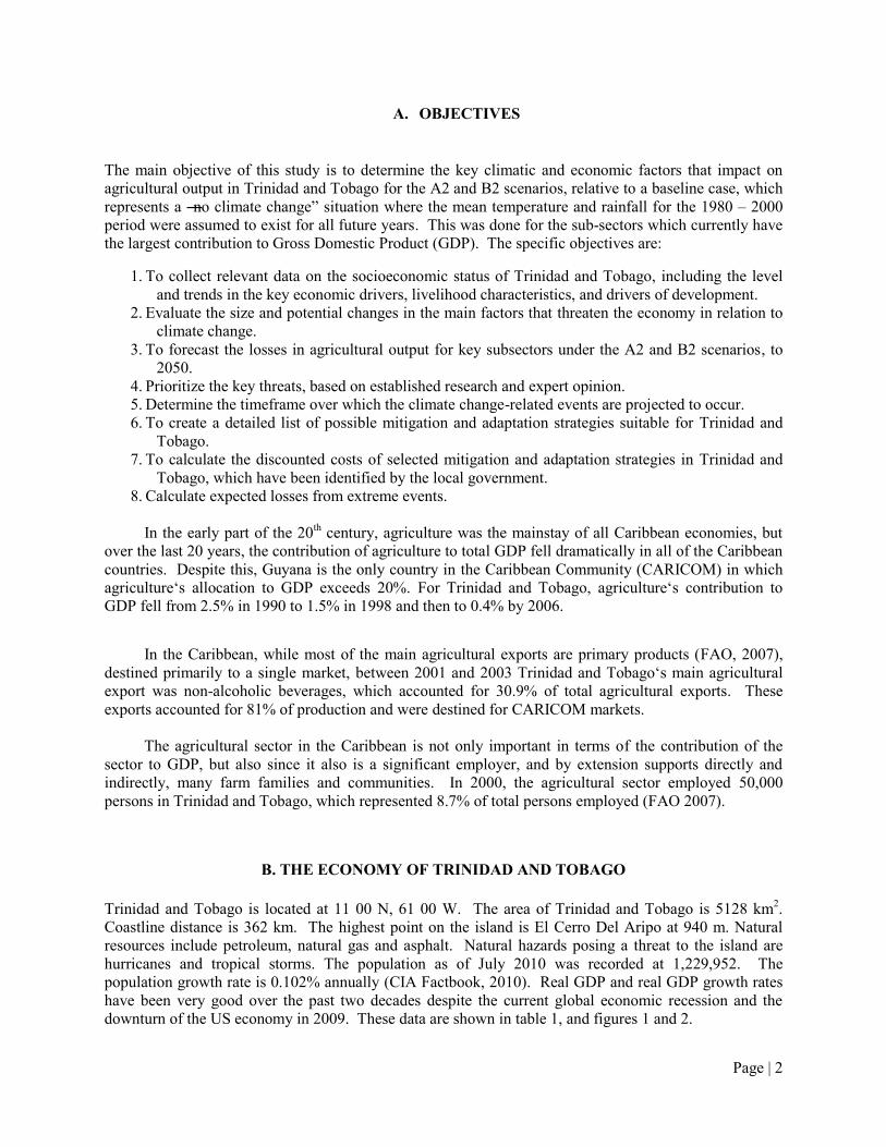
B. THE ECONOMY OF TRINIDAD AND TOBAGO Trinidad and Tobago is located at 11 00 N, 61 00 W. The area of Trinidad and Tobago is 5128 km2. Coastline distance is 362 km. The highest point on the island is El Cerro Del Aripo at 940 m. Natural resources include petroleum, natural gas and asphalt. Natural hazards posing a threat to the island are hurricanes and tropical storms. The population as of July 2010 was recorded at 1,229,952. The population growth rate is 0.102% annually (CIA Factbook, 2010). Real GDP and real GDP growth rates have been very good over the past two decades despite the current global economic recession and the downturn of the US economy in 2009. These data are shown in table 1, and figures 1 and 2.

Page | 3

Table 1: Real GDP Growth Rate of Trinidad and Tobago

Year Real GDP Growth Rate% Real GDP Figure (Factor Costs)

1996 7.09 3.2 1997 7.32 2.9 1998 7.48 4 1999 8.98 5.1 2000 7.25 4.7 2001 4.2 3.5 2002 7.92 2.7 2003 14.4 3.4 2004 7.8 4.2 2005 5.8 10 2006 13.4 12.2 2007 4.8 4.6 2008 2.4 2.3 2009 -3.5 0.9

Figure 1: Real GDP Growth Rate of Trinidad and Tobago (%)

Source: Central Bank of Trinidad and Tobago (1999, 2000, 2007)

Figure 2: Real GDP (at Factor Cost) of Trinidad and Tobago


Page | 4

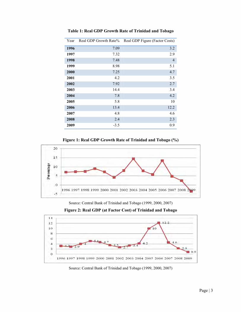
Inflation rates in Trinidad and Tobago increased steadily since 2004 (figure 3), fuelled primarily by a significant rise in local food prices, which in some respects mirrored increases in food prices on the global market, but which in general, reflected local market inefficiencies. This significant inflation rate is important in assessing the performance of the agricultural sector, because the rise in prices affects not only the prices of retail goods that consumers face, but since most of the inputs to the agricultural sector are imported, high inflation also increases the cost of production.

Figure 3: Inflation Rate in Trinidad and Tobago (%)


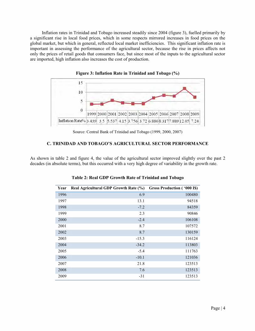
C. TRINIDAD AND TOBAGO’S AGRICULTURAL SECTOR PERFORMANCE As shown in table 2 and figure 4, the value of the agricultural sector improved slightly over the past 2 decades (in absolute terms), but this occurred with a very high degree of variability in the growth rate.

Table 2: Real GDP Growth Rate of Trinidad and Tobago

Year Real Agricultural GDP Growth Rate (%) Gross Production ( ‘000 I$) 1996 6.9 100480 1997 13.1 94518 1998 -7.2 84359 1999 2.3 90846 2000 -2.4 106108 2001 8.7 107572 2002 8.7 130159 2003 -15.3 116124 2004 -34.2 113803 2005 -5.4 111763 2006 -10.1 121036 2007 21.8 123513 2008 7.6 123513 2009 -31 123513

Page | 5

Figure 4: Agricultural GDP and Associated Growth Rate for Trinidad and Tobago


As shown in figures 5 and 6, the economy of Trinidad and Tobago became more and more dependent of revenue from the petroleum sector over time, while at the same time, the contribution of the agricultural sector fell from 2% of total GDP in 1997 to just 0.4% of total GDP in 2009.

Figure 5: Percentage Contribution to GDP by Sector in Trinidad and Tobago, 1997


Page | 6

Figure 6: Percentage Contribution to GDP by Sector in Trinidad and Tobago, 2009


Even though the forested area in Trinidad and Tobago fell by 5.3% between 1990 and 2008 (table 3), arable land availability fell by 35.6% over that time, and the available agricultural land fell by 29.9%, which would have a significant impact on total potential production.

Table 3: Agricultural and Forest Land Area (1000 Hectares) and Tractor Use, Selected Years

Year 1980 1990 2000 2008 Agricultural Land Area 101,00 77,00 67,00 54,00 Arable Land Area 60,00 36,00 35,00 25,00 Permanent Crops Area 35,00 35,00 25,00 22,00 Forested Area n\a 240,70 233,60 227,84 Total Area Equipped for Irrigation 3,00 4,00 5,00 7,00

Source: FAOSTAT

In 2008, the labour force in the agricultural sector accounted for 3.8% of all industries (Central Bank of Trinidad and Tobago, 2009). While this is a small number which represents direct employment, there is anecdotal evidence that the local agricultural sector supports a very large informal or indirect sector, particularly of the rural population. Therefore, agricultural employment is still very critical, despite its low contribution to national GDP, in terms of supporting rural livelihoods, and providing employment to many unskilled workers. Agricultural output is also increasingly significant as global food prices continue to increase and the Trinidad and Tobago government looks to increasing food security amidst a spiraling food import bill.

Agricultural land area was 84,990 ha, of which 56.4% were cultivated croplands. In 1980, the largest components of the agricultural sector were the sugar sub-sector, followed by domestic agriculture and then export agriculture. However, following the closure of the main sugarcane producing farm

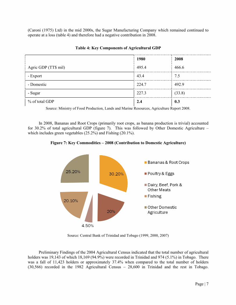
Page | 7

(Caroni (1975) Ltd) in the mid 2000s, the Sugar Manufacturing Company which remained continued to operate at a loss (table 4) and therefore had a negative contribution in 2008.

Table 4: Key Components of Agricultural GDP

1980 2008

Agric GDP (TT$ mil) 495.4 466.6

- Export 43.4 7.5

- Domestic 224.7 492.9

- Sugar 227.3 (33.8)

% of total GDP 2.4 0.3 Source: Ministry of Food Production, Lands and Marine Resources, Agriculture Report 2008.

In 2008, Bananas and Root Crops (primarily root crops, as banana production is trivial) accounted

for 30.2% of total agricultural GDP (figure 7). This was followed by Other Domestic Agriculture – which includes green vegetables (25.2%) and Fishing (20.1%).

Figure 7: Key Commodities – 2008 (Contribution to Domestic Agriculture)


Preliminary Findings of the 2004 Agricultural Census indicated that the total number of agricultural holders was 19,143 of which 18,169 (94.9%) were recorded in Trinidad and 974 (5.1%) in Tobago. There was a fall of 11,423 holders or approximately 37.4% when compared to the total number of holders (30,566) recorded in the 1982 Agricultural Census – 28,600 in Trinidad and the rest in Tobago.

Page | 8

Individual/Household/Sole Proprietor and Joint Partnerships accounted for 99.5% of all holders (GORTT, CSO, 2005).

Most of the holders, 13,874 or 72.4% were engaged in Crop Production (figure 8). Ninety six percent (96.0%) of all holdings were less than ten (10) hectares in area, with an average size of a Private Holder‘s household being 4.2 persons. Twenty two percent (22.0%) of all holdings were less than 0.5 hectares, 65.1% were between 0.5 and less than 5 hectares, 8.9% between 5 and 10 hectares, while only 4.0% were greater than 10 hectares in size.

The male/female ratio of holders was found to be 5.9: 1, and only forty percent (40.0%) of the Private Holders were registered under the Farmers Registration Programme of the Ministry of Agriculture, Lands and Marine Resources.

Figure 8: Holders in Trinidad and Tobago by Type of Agricultural Activity

Source: GORTT, CSO (2005), figure 1

Most of the farms (89.4%) were concentrated in six regions. The region of Couva/Tabaquite/Talparo recorded the highest number with 3,078 holders. There were 2,812 holders in the region of Princes Town, 2,099 in Mayaro/Rio Claro, 2,460 in Sangre Grande, 2,227 in Penal/Debe, 2,221 in Tunapuna/Piarco and 1,342 holders were in the region of Siparia (figures 9 and 10).

In 2004, Private Holders accounted for 19,055 or approximately 99.5% of which 18,505 were classified as ―Individual/Household/Sole Proprietor‖ and 550 as ―Joint Partnership‖. The remaining 0.5% of holdings was primarily Private Companies and Government Institutions. The percentage of Private Holders was the same in 1982.

Page | 9

Figure 9: Distribution of Holders by Type of Agricultural Activity and Parishes in Trinidad

Source: GORTT, CSO (2005), Map 1

Figure 10: Distribution of Holders by Type of Agricultural Activity and Parishes in Tobago

Source: GORTT, CSO (2005), Map 2

Page | 10

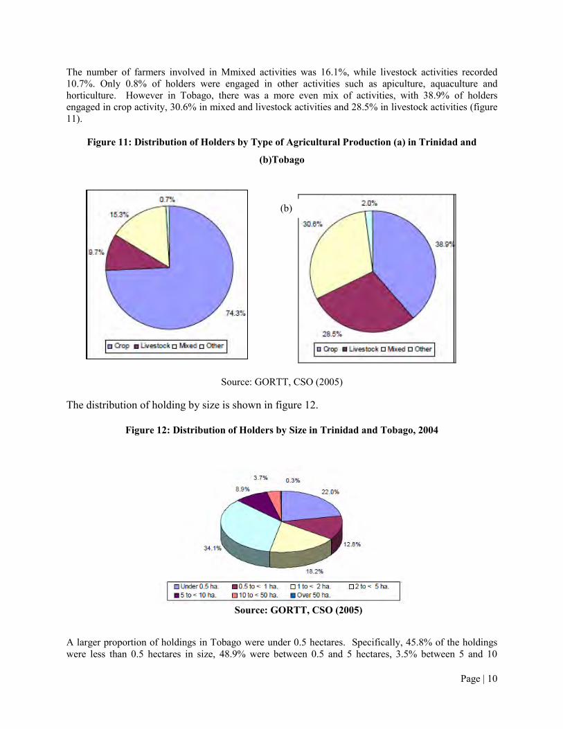
The number of farmers involved in Mmixed activities was 16.1%, while livestock activities recorded 10.7%. Only 0.8% of holders were engaged in other activities such as apiculture, aquaculture and horticulture. However in Tobago, there was a more even mix of activities, with 38.9% of holders engaged in crop activity, 30.6% in mixed and livestock activities and 28.5% in livestock activities (figure 11).

Figure 11: Distribution of Holders by Type of Agricultural Production (a) in Trinidad and

(b)Tobago

Source: GORTT, CSO (2005)

The distribution of holding by size is shown in figure 12.

Figure 12: Distribution of Holders by Size in Trinidad and Tobago, 2004


A larger proportion of holdings in Tobago were under 0.5 hectares. Specifically, 45.8% of the holdings were less than 0.5 hectares in size, 48.9% were between 0.5 and 5 hectares, 3.5% between 5 and 10

(b)

Page | 11

hectares while only 1.8% were greater than 10 hectares in size. The distribution of farmers by age group is shown in figure 13. Approximately two-thirds of all farmers were at least 45 years old.

Figure 13: Distribution of Holders by Age Group in Trinidad and Tobago, 2004


D. PHYSICAL AND SOCIO-ECONOMIC VULNERABILITIES OF THE CARIBBEAN

The Caribbean region is more vulnerable than many other Least Developed Countries (LDCs) when hurricanes and tropical storms strike, as the coast exposure is very high, relative to land mass (FAO 2007). In addition, hurricanes not only cause severe damage, but occur with a high frequency in the region. In addition, vulnerability is increased as a significant portion of the arable land in the Caribbean exists on steep slopes, which make them susceptible to soil erosion. Compared to LDCs, the per capita arable land availability is about half, which, with the difficulty of achieving economies of scale due to the small populations and the productivity of agricultural production declined over time.

―As barriers to world trade are dismantled, the most competitive producers increase their market share. Caribbean economies have low levels of competitiveness due to higher unit costs of production (caused by scarce resources, high transport costs, low economies of scale, small size of firms, etc.) and thus their market share will decrease under the new conditions.‖ FAO (2007)

Also, as a result of limited production diversity, most of the inputs needed for agricultural production, such as machinery, fertilizers and pesticides are imported, which further raises the vulnerability of the agricultural sector.

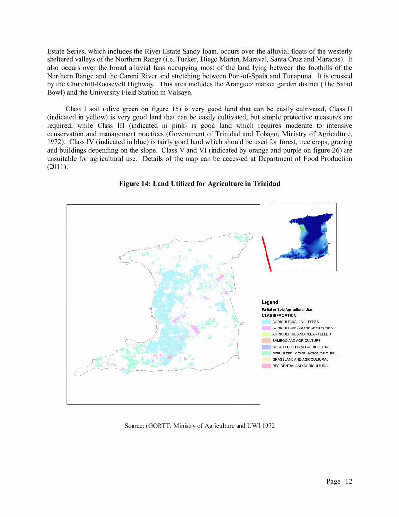
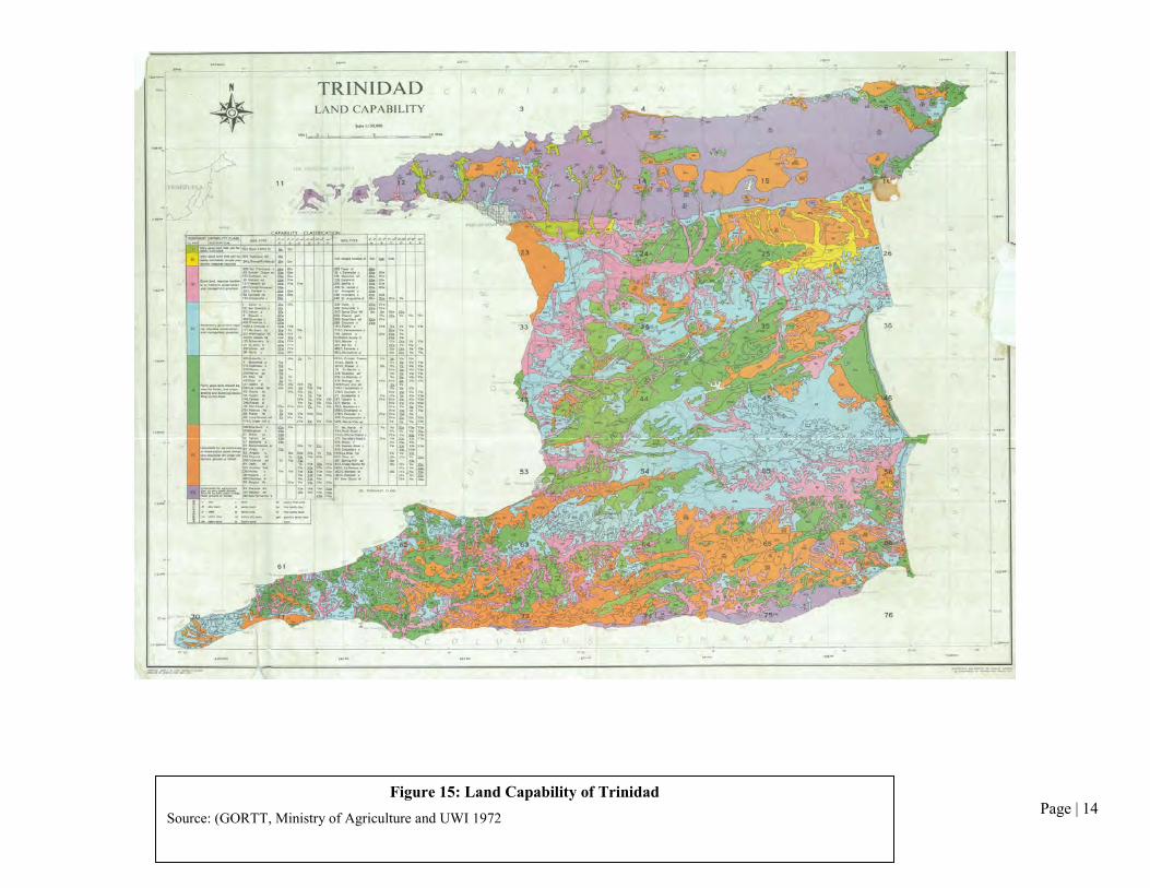
1. Land Capability

Land under various agricultural uses in Trinidad is shown in figure 14. Soil types and land capability are quite diverse in Trinidad and Tobago. Based on the work by Hardy (1977), land capability in Trinidad is divided into 7 classes. The best type of land is Class I, which is the River Estate Sandy Loam. The River

Page | 12

Estate Series, which includes the River Estate Sandy loam, occurs over the alluvial floats of the westerly sheltered valleys of the Northern Range (i.e. Tucker, Diego Martin, Maraval, Santa Cruz and Maracas). It also occurs over the broad alluvial fans occupying most of the land lying between the foothills of the Northern Range and the Caroni River and stretching between Port-of-Spain and Tunapuna. It is crossed by the Churchill-Roosevelt Highway. This area includes the Aranguez market garden district (The Salad Bowl) and the University Field Station in Valsayn.

Class I soil (olive green on figure 15) is very good land that can be easily cultivated, Class II

(indicated in yellow) is very good land that can be easily cultivated, but simple protective measures are required, while Class III (indicated in pink) is good land which requires moderate to intensive conservation and management practices (Government of Trinidad and Tobago, Ministry of Agriculture, 1972). Class IV (indicated in blue) is fairly good land which should be used for forest, tree crops, grazing and buildings depending on the slope. Class V and VI (indicated by orange and purple on figure 26) are unsuitable for agricultural use. Details of the map can be accessed at Department of Food Production (2011).

Figure 14: Land Utilized for Agriculture in Trinidad

Source: (GORTT, Ministry of Agriculture and UWI 1972

Page | 13

Page | 14

Figure 15: Land Capability of Trinidad Source: (GORTT, Ministry of Agriculture and UWI 1972

Page | 15

II. CLIMATE CHANGE IMPACTS ON AGRICULTURE

Potential impacts of climate change on agriculture are quite varied. A summary of key potential climate impacts are shown in table 5 below.

Table 5: Climate Change and Related Factors Relevant to Agricultural Production at the Global Scale

Source: Iglesias and others (2009)

While many early climate models predicted very severe impacts on the world‘s food supply, more

recent models have indicated there will be very negative impacts in some areas, especially in the tropics and in areas vulnerable to changes such as sea level rise, and in areas heavily dependent on rain fed agriculture (rural areas) for the sustenance for their livelihoods (Antle, 2008). In many of these cases, incomes are very low, and there is a high dependence on agriculture. However, it is also likely that there will be positive impacts, particularly in upland tropical and temperate regions. So as food supply increases in some areas, this could offset the negative impacts in other areas via price reductions and international trade. Globally overall, the impacts of climate change may well be positive (Antle, 2008).

Cline (2007) however, indicated that aggregate world agricultural impacts of climate change will be negative, though moderate, by late this century, which contradicts the view that world agriculture

Page | 16

would actually benefit in the aggregate from business as usual global warming over that horizon. What is consistent, and key for the Caribbean, is that his work, like previous research agrees that damage will be disproportionately concentrated in developing countries. Further analysis therefore needs to assess the projected increases in temperature (and changes in rainfall) to add further information on potential impacts on production. Crop specific climate impacts such as these, are also discussed in Box 1.

Box 1: Crop Responses to Changing Climate

Source: U.S. Global Change Research Program (2009)

III. LITERATURE REVIEW

A. MODELS Several approaches have been used to assess the impact of climate change on the agricultural sector. In some cases, impacts were measured in relation to specific dominant commodities, and other cases, the impact was measured on country – level impacts. Most of the models can be classified as:

1. Ricardian Models 2. Panel/Fixed Effects Models

Crop responses in a changing climate reflect the interplay among three factors: rising temperatures, changing water resources, and increasing carbon dioxide concentrations. Warming generally causes plants that are below their optimum temperature to grow faster, with obvious benefits. For some plants, such as cereal crops, however, faster growth means there is less time for the grain itself to grow and mature, reducing yields.193 For some annual crops, this can be compensated for by adjusting the planting date to avoid late season heat stress.164 The grain-filling period (the time when the seed grows and matures) of wheat and other small grains shortens dramatically with rising temperatures. Analysis of crop responses suggests that even moderate increases in temperature will decrease yields of corn, wheat, sorghum, bean, rice, cotton, and peanut crops. Some crops are particularly sensitive to high nighttime temperatures, which have been rising even faster than daytime temperatures. …. Further, as temperatures continue to rise and drought periods increase, crops will be more frequently exposed to temperature thresholds at which pollination and grain-set processes begin to fail and quality of vegetable crops decreases. …Higher temperatures will mean a longer growing season for crops that do well in the heat, such as melon, okra, and sweet potato, but a shorter growing season for crops more suited to cooler conditions, such as potato, lettuce, broccoli, and spinach. Higher temperatures also cause plants to use more water to keep cool. …But fruits, vegetables, and grains can suffer even under well-watered conditions if temperatures exceed the maximum level for pollen viability in a particular plant; if temperatures exceed the threshold for that plant, it won‘t produce seed and so it won‘t reproduce.

Page | 17

3. Agroeconomic Models 4. Agroecological Models 5. Crop Production Functions

Ricardian Models (Cross-Sectional Reduced-Form Hedonic Pricing Models) By far, most of the literature has focused on the use of Ricardian Models. These models look at the impact of climate change on farm land value or net farm income. Theoretically, it is assumed that changes in farm output in terms of the quantity of products or the value of products, together with the opportunity cost of the land is reflected in the farm‘s land value. Farmland net revenues reflect net productivity. In addition, ―the value of a parcel of land should reflect its potential profitability, implying that spatial variations in climate derive spatial variations in land uses and in turn land values.‖ Its clear advantage is that if land markets are operating properly, prices will reflect the present discounted value of land rents into the infinite future (Deschenes and Greenstone, 2006). In this case, farm land value is usually seen as dependent on output prices, labour costs, the level of capital investment, climate variables such as rainfall and temperature, and soil characteristics.

In addition, the effects are often modeled in terms of differences in the projected response of agricultural systems that are either rain fed or irrigated. This model has been used primarily for agricultural systems in Africa (Kurukulasuriya and Mendelsohn, 2008a; Kurukulasuriya and Mendelsohn (2008b), Sri Lanka (Seo, Mendelsohn and Munasinghe, 2005; Deressa and Hassan 2009; Molua and Lambi, 2007; Deressa, Hassan and Poonyth, 2005; Maddison, Manley and Kurukulasuriya, 2007; Seo and Mendelsohn, 2006; Kurukulasuriya and others, 2006), Latin America (Seo and Mendelsohn, 2008; Seo and Mendelsohn, 2007), and the US (Schlenker and others, Fisher, 2005).

The main strength of this model is that it incorporates the possibility of farmers adapting to climate change over time, using a number of mechanisms such as changing the type of crops or livestock farmed, changing crop varieties or livestock breeds, changing sowing times (in response to changing climatic conditions), or changing their production systems (by employing additional and/or different hard or soft technologies). Since farm-level data are used, the impact of climate change in the Ricardian model is determined from the changes in farm output from farms which are located in wide variety of climatic zones (with distinct variations in soil and climate parameters).

Based on work in Zimbabwe by Mano and Nhemachena (2007), which utilized surveys of 700 smallholder farm households, temperature and precipitation were found to have significant impacts on net farm revenues. Net farms incomes were negatively affected by temperature increases and benefitted from increases in rainfall. Seo, Mendelsohn and Munasinghe (2005) also found similar temperature and precipitation effects in Sri Lanka. Further, based on sensitivity analysis, net farm incomes for farms which utilized rain fed systems were very sensitive to changes in these climatic variables, relative to irrigated farms. This suggested that irrigation is an important adaptation strategy in the face of climate change. It was also discovered that farmers in Zimbabwe were already adapting to climate change by planting drought-resistant crops, changing planting dates and using irrigation.

A criticism of this model is that it may fail to include other variables that are also expected to affect farm net incomes, such as market access and soil quality, but for which data may be scarce. In such cases, the model may be subject to misspecification errors. In a climate change scenario, it is likely that agricultural output levels will change, which will affect prices. Since the Ricardian model also assumes that prices remain constant, this is another limitation, so that damages may be understated (as potential price drops are ignored) and benefits could be overstated (as increased supply values are inflated) (Mano

Page | 18

and Nhemachena, 2007). The method also cannot measure the effect of variables that do not vary across space such as CO2 (Seo, Mendelsohn and Munasinghe, 2005).

Another flaw of the Ricardian model is that it is static and therefore assumes that technology, policy and land use (which all have significant impacts on farmers‘ production decisions) do not change. In a country like Zimbabwe, the model also does not always take into account the potential for water supply, whether within or outside the country borders, and instead relies in rainfall impacts only. This is seen as another shortcoming. Therefore in the study by Mano and Nhemachena (2007), runoff is taken as a proxy for surface water availability.

Once the relationship between climatic and other independent variables on net farm income was

established, projections for various global climate scenarios were then undertaken. Seo, Mendelsohn and Munasinghe (2005) confirms that based on their research findings for Sri Lanka, and the findings of others, climate change damage could be large in tropical developing countries, but highly dependent on the actual climate scenario. Analyses that do not include efficient adaptation (such as the early agronomic studies) overestimate the damage associated with any deviation from the optimum. Adaptation can explain the more optimistic results found with the Ricardian method compared to more pessimistic results found in purely agronomic studies (Kurukulasuriya and Mendelsohn, 2008a).

Panel/Fixed Effects Models

The Ricardian model was also extended to a panel data model (Polsky, 2004), which may also be conditional on county and state by-year fixed effects, for assessing the impact of climate in the United States of America (Deschenes and Greenstone 2006). They found that the predicted increases in temperature and precipitation will have virtually no effect on yields among the key crops (corn for grain, soybeans, and wheat), even though there is a wide disparity in the results across states, with some states suffering significant losses, while others benefitting from climate change.

―This approach differs from the hedonic one in a few key ways. First, under an additive separability assumption, its estimated parameters are purged of the influence of all unobserved time invariant factors. Second, it is not feasible to use land values as the dependent variable once the county fixed effects are included. This is because land values reflect long run averages of weather, not annual deviations from these averages, and there is no time variation in such variables. Third, although the dependent variable is not land values, our approach can be used to approximate the effect of climate change on agricultural land values. Specifically, we estimate how farm profits are affected by increases in temperature and precipitation. We then multiply these estimates by the predicted changes in climate to infer the impact on profits. Since the value of land is equal to the present discounted stream of rental rates, it is straightforward to calculate the change in land values when we assume the predicted change in profits is permanent and make an assumption about the discount rate.‖ (Deschenes and Greenstone 2006).

This approach was also applied in Deschenes and Greenstone (2004, 2007). Agronomic-Economic Crop Models This approach to modeling climate change impacts in agriculture uses well-calibrated crop models from carefully controlled experiments in which crops are grown in field or laboratory settings that simulate different levels of precipitation, temperature and carbon dioxide. Under these conditions, farming methods are not allowed to vary and farmers‘ adaptation to changing climate cannot be captured in these

Page | 19

models. Scientists are able to estimate a yield response of specific crops to various conditions. The presumed changes in yields from the agronomic model are fed into an economic model, which determines crop choice, production, and market prices.

Rosenzweig and Parry (1994) predicted that doubling of atmospheric carbon would have only a small negative effect on global crop production, but the effects would be more pronounced in developing countries. Cline (2007) predicted overall significant falls in overall yields in Sub-Saharan Africa, using various global circulation models. Parry and others (2004) used this approach to estimate the potential impacts of climate change on global food production for the A1FI, A2, B1, and B2 IPCC climate change scenarios developed from the HadCM3 global climate model. (Finger and Schmid, 2007) also used an agronomic model to analyze corn and winter wheat production on the Swiss Plateau with respect to climate change scenarios. Yield functions were also modeled by Furuya, S. Kobayashi, and S. D. Meyer (2009), using subsidized producer price, and a time trend, in addition to temperature and precipitation variables. Agro-Ecological Zone Models (also called the crop suitability approach) In this case, crops are categorized into various agro-ecological zones and yields are then predicted. These models combine crop simulation models with land-use decision analysis and model changes in inputs and climate variables to assess changes in agricultural production, assuming that lands can shift from one agro-ecological classification to another with changes in environmental conditions (Cline, 2007). The agro-ecological models examine changes in agro-ecological zones and crops as climate changes and predict the effect of alternative climate scenarios on crop yields. Economic models then use the projected changes in yields to predict the overall supply effects.

One of the biggest advantages associated with agroecological zones is that the geographic distribution of the zones in [many] developing countries has been published (Mendelsohn and Dinar, 1999). However, there are still many problems. The climate zones usually represent large temperature categories, so that subtle shifts within a zone have no effect but a small shift from one zone to another has a dramatic consequence. Further, the effects of soils and climate are computed independently, which ignores the interrelationship of these variables. Here, as with the agroeconomic models, researchers must explicitly account for adaptation. Large price changes along with small changes in aggregate supply have often been found, indicating that there may be problems with the calibration of the underlying economic model (Mendelsohn and Dinar, 1999).

Some of the models have also been developed at the global scale, such as Golub, Hertel and Sohngen (2007), who estimated a linked supply and demand model for global land using a dynamic general equilibrium (GE) model that predicts economic growth in each region of the world, based on exogenous projections of population, skilled and unskilled labour and technical change, and that differentiate the demand for land by Agro-Ecological Zone (AEZ).

Crop Production Functions

Production function models generally link the outputs of crops or livestock as functions of inputs to the production process, such as land, labour, capital and entrepreneurial skill. These inputs can be incorporated individually, or as an index, such as the Laspeyres Quantity Index, which can combine any physical inputs together. As was shown for Spain by Quiroga Gómez and Iglesias (2005), these types of models utilized panel data to estimate the relationship between production (such as tonnes per hectare) as a function of socio-economic and climate variables in various agro-climatic zones. In this case, not only was the impact of mean temperature analyzed, but also the impact of maximum temperature, minimum

Page | 20

temperature and years for which annual rainfall fell below the mean (considered to be ―dry‖ years) for the period under consideration. In addition, the impact of various technological variables were also included such as machinery value, fertilizer use, pesticide imports, and percentage irrigated land for production of wheat, grapes, olives and oranges.

While the production function approach is the least common approach used to model the impacts of climate change on agricultural outputs to date, it is empirically sound. According to Deschenes and Greenstone (2006), the production function approach provides estimates of weather effects on crop yields that do not include bias due to agricultural output factors such as soil quality that are beyond farmers‘ control. On the other hand, these authors noted that a disadvantage is that production function estimates do not account for the full range of adaptation responses that farmers can make to changes in weather in order to maximize their profits. Since farmer adaptations are completely constrained in the production function approach, it is likely to produce estimates of climate change that are biased downwards.

JieMing, WenJie and DuZheng (2007) evaluated the impact of climate changes on grain yields in China, using the Cobb-Douglas production function. In this study, a monthly climate drought index was calculated (i.e. the monthly rainfall anomaly divided by the normal of this monthly rainfall), together with a climate input indicator to analyze and verify the relationship between yearly grain yield and yearly key month drought index.

One advantage of the production function approach is that historical farm-level and aggregated data take into account farmers‘ historical reactions to changes in climatic and economic conditions. However, these historical data are not able to capture future plant-climate interactions in a sufficient manner, especially where the crop-weather relationship is restricted to a few variables such as temperature and rainfall. In addition, these models cannot sufficiently integrate expected CO2 fertilization effects on plants due to low variation in historical CO2 concentrations (Finger and Schmid 2007).

Gay and others (2006) determined the relation between coffee production in Veracruz, Mexico and economic and climatic variables. The model showed that temperature was the most relevant climatic factor for coffee production, and that coffee production might not be economically viable for producers, since the model predicts a fall in production by 34%. The model used mean seasonal temperature, mean seasonal precipitation, and the seasonal variance of climatic variables. In addition, economic variables such as state and international coffee prices, a producer price index for raw materials for coffee, and national and United States of America coffee stocks were considered as well as the state real minimum wage, as a proxy for the price of labour employed for coffee production. These variables however, were not all modeled at the same time, due to the limited number of production data. Gay and others (2006) suggested that other explanatory variables could be used to assess climate change impacts on cop production. These include: seasonal averages of precipitation and temperature (linear and quadratic), their variations from a 20 year mean value, the percentage of full-time farm households, land slope and a time trend to account for technology changes.

Other models utilized economy-wide, global computable general equilibrium models such as the one used by Zhai, Lin, and Byambadorj (2009) who computed the impacts of climate change on the Republic of China‘s agricultural sector. Bosello and Zhang (2005) also used a global general equilibrium model.

Summary

Page | 21

All of the above mentioned models were theoretically appropriate for use in modeling agricultural production in Trinidad and Tobago; however, given that household level data on output, prices and input use were not available, the utilization of the Ricardian model, the fixed effects model and agroeconomic model could not be used in this study. Therefore, only the production function approach was considered.

B. DATA

1. Climate Data Monthly total rainfall and mean temperature data were obtained from the Trinidad and Tobago Central Statistical Office. Annual rainfall data were available for 1940 - 2008 and temperature data for 1946 - 2008. For the Providing Regional Climates for Impact Studies (PRECIS) model the mean annual rainfall and mean monthly temperature were 771 mm and 26.22 C respectively. Based on historical data for Trinidad and Tobago, the mean annual rainfall and mean monthly temperature were 1920 mm and 26.7 C respectively. Since there was a large difference between the historical means for rainfall and the PRECIS estimates, and based on the advice of the Institute of Meteorology (INSMET) in Cuba via personal communication, the model anomalies were used. The European Center Hamburg Model (ECHAM) anomalies for the estimated A2 and B2 climate variables were added to the mean historical rainfall and temperature for 1961-1990, the same period used as the base period in the ECHAM model, to determine the future climate levels under the A2 and B2 scenarios.

2. Root Crop and Vegetable Data The area under traditional cultivation for green vegetables and root crops was given in hectares, and was obtained from various Food Crop Bulletins, Quarterly Agricultural Reports and issues of the Agricultural Report (GORTT, CSO, 2005). The category of green vegetables was made up of 17 items: tomato, cabbage, cucumber, melongene, bodi, ochro, lettuce, pumpkin, patchoi, water melon, sweet peppers, celery, cauliflower, chive, hot peppers, dasheen bush and sorrel, as presented in the Agricultural Report3. The category of Root Crops was made up of 7 items: cassava, dasheen, yam, tannia, eddoes, ginger and sweet potato, as presented in the Agricultural Report4. This information was sought on a monthly basis from 1995 to 2008 for Trinidad only5. The quantity of harvest and price data were available for almost all months, but only 77% of the data were consistently available for area under cultivation for green vegetables and root crops.

The quantity of root crops and green vegetables was the estimated annual quantity of the commodities harvested from traditional cultivation only for Trinidad. These data were all converted to thousands of kg, using conversion factors provided by the National Marketing and Development

3 However, sorrel was omitted since its production was largely based on day length and most of the months had no data as the production is highly seasonal. Therefore, only 16 green vegetable commodities were modeled.

4 However, yam and tannia were omitted from the analysis as there was a significant portion of missing area, price and quantity data (>60%), and with very limited variability in the available data. Therefore, only 5 root crops were modeled.

5 Very little time series data were available for Tobago, so Tobago vegetable and root crop production could not be included in the analysis.

Page | 22

Company (NAMDEVCO) for the cases where quantities were presented as bundles, singles or heads, as in the case of some commodities such as lettuce. Nominal prices were obtained as the annual average food crop price received by farmers for traditional food crops, and again converted to $/kg when other price units were used. Based on this, a weighted price for root crops was calculated as the sum of all root crop values divided by total quantity of root crops harvested. The same approach was used to calculate a weighted price for green vegetables.

Based on personal communication with the CSO, prices reported for green vegetables and root crops refer to wholesale prices, and bundles (for celery, chive, bodi, dasheen bush and patchoi), were large bundles. In 2004, no surveys were done during November and December, in preparation for the nationwide census. In 2006, CSO reported that due to technical difficulties, no surveys were conducted for the year; therefore monthly data on yield and acreage were not available for this year.

Prior to July 2005, data on agricultural surveys or recordings of agricultural activity were not available for Tobago. NAMDEVCO‘s price data for 2006 and 2007 for the green vegetables and root crops were used as proxies. CSO reported that NAMDEVCO separates the prices for green vegetables (small, medium and large) and root crops (local and imported) whereas CSO takes the average for each.

Missing data (assumed to be zero-values) for green vegetables‘ quantity were replaced by the quantity of the crop in the previous year, for the same month. Missing data for green vegetables‘ prices used the same approach as that for missing quantities. The relative weights of the area under cultivation for 7 years in which all the year‘s data were available, were averaged. These weights were then applied to the real area data for the years in which 6 months (odd months) data were available. For 2003 where November and December data were missing, the previous year‘s data were used as proxies. Where zero values still existed, the previous year‘s data were used as proxies. The same approach was used for root crops.

Data on monthly imports of agricultural pesticides and machinery which can be used for vegetable and root crop production and fertilizers (all measured in kgs) and their associated values (measured in mil TT$), were obtained from CSO. These data were used to estimate a Laspeyres Quantity Input Index as a proxy for agricultural input use for that month, since data on actual inputs used at the farm level were not available. The effects of tropical storms on production were not modeled since the incidence of these events in Trinidad and Tobago was extremely low for the sample period utilized. The annual Consumer Price Index (CPI) for Trinidad and Tobago was obtained from NationMaster.Com (2010) for 1970-2005 and the monthly Consumer Price Index (CPI) for Trinidad and Tobago was obtained from the World Bank‘s statistical database for 1995-2008. Real prices were calculated using the CPI, with 2008 as the base year.

3. Cocoa The quantity of cocoa was the deliveries to principal exporters (in thousands of kgs), which was used as a proxy for production. The cocoa price used the average export price ($/kg). All the cocoa data were taken from Agricultural Reports for a variety of years.

4. Fisheries6 Data on the quantity of fish landed (kg), the associated value (TT$) and number of trips7 were obtained

6 Fisheries data was sought from the Fisheries Division of the Tobago House of Assembly. Permission was granted to access the data, however due to technical difficulties access was not possible.

Page | 23

from the Fisheries Division, Ministry of Food Production, Land, and Marine Affairs, Trinidad and Tobago, on a monthly basis from 1996 – 2008. These data accounted for all gear and species from Trinidad Artisanal Fleets (nets, lines and trawl) and the Trinidad Semi-Industrial Trawl fleet8. These data were used as it represented the vast majority of landings (see Appendix 1). In addition, available data on the Tobago fisheries were estimates with little variation over time, and data on other fleets were for very short time periods. From this source, the value of these landings was based on ex-vessel prices.

IV. METHODOLOGY

Based on a Production function framework, models for each of the four sub-sectors were initially estimated using an Ordinary Least Squares (OLS) approach. The assumption was that production is a function of land, capital, price of the output and climate variables (mean temperature and rainfall). A double log specification was employed for all variables. The squared climate variables were included as it was assumed that the effect of increasing levels of these variables exhibited diminishing returns. Each variable was tested for the presence of unit roots, and any serial correlation detected was corrected using ARMA models for each subsector, based on Q-statistics and the Breusch-Godfrey Serial Correlation LM Test. Models were also tested for the presence of heteroscedasticity using the Breusch-Pagan Godfrey heteroscedasticity test and White‘s test for heteroscedasticity.

A. MODELS Root Crops LOG(QR) = 1 + 2 LOG(RPR) + 3 (ARC) + 4 LOG(LASQIND) + 5 LOG(TEMP) + 6 LOG(TEMP)

2 + 7 LOG(RAIN) + 8 LOG(RAIN)

2 + 9 DRY + + 10 TREND

Where QR = quantity of root crops harvested (‗000kg)

RPR = Real weighted root crop prices ($/kg)

ARC = Area of root crops (hectares)

LASQIND = Laspeyres Quantity Index

Temp = mean monthly temperature ( C)

Rain = mean monthly rainfall (mm)

Dry = Dummy variable, shown as 1 during the dry season (January - May) and 0 otherwise.

Trend = monthly linear time trend

7 Trips for a particular species for a particular gear refer to trips of that gear that caught the species. Landings/trip and Value/Trip for a particular species for a particular gear is calculated using the total trips done by the gear and not the number of trips that caught the species. Trips are not standardized across gears.

8 These data do not include landings from the Trinidad semi-industrial multi-gear boats, industrial Trawling and Longline Fleet, Trinidad recreational boats, Tobago landings, and any landings from foreign fleets that may have operated in Trinidad and Tobago waters.

Page | 24

Cocoa LOG(QC) = 1 + 2 LOG(PCR) + 3 LOG(TEMP) + 4 LOG(TEMP)

2 + 5 LOG(RAIN) + 6

LOG(RAIN) 2 +

Where QC = quantity of cocoa exported (‗000kg)

PCR = Real cocoa export price ($/kg)

Green Vegetables

LOG(QVEG) = 1 + 2 LOG(RPVEG) + 3 (AVEG) + 4 LOG(FIMQ) + 5 LOG(TEMP) + 6

LOG(TEMP) 2 + 7 LOG(RAIN) + 8 LOG(RAIN)

2 +

Where QVEG = quantity of green vegetables harvested (‗000kg)

RPVEG = Real weighted green vegetable prices ($/kg)

AVEG = Area of green vegetables (hectares)

FIMQ = Quantity of Imported Fertilizer

For the green vegetables and root crops sub-sectors, a common Laspeyres Quantity Index was calculated using three components: monthly quantity of machinery, pesticide and fertilizer imports and associated values. Values for fertilizers and pesticides were available from 1995-2008, but machinery data for 1995 were largely zero valued, and could not be validated, therefore, the index was calculated as a proxy for input use from 1996-2008.

Laspeyres Quantity Index= n

i

titi

n

i

titi

QP

QPn

1,,

1,,

00

0

where the index measures the change in price, with to representing the base period, tn represents the current period and i represents machinery, pesticides and fertilizers.

B. RESULTS AND FORECASTS

1. Key Model Variables For the root crops and green vegetables, the base period of 1995-2008 was used, with the descriptive statistics for quantity, area, real average weighted price and climate variables provided in table 6.

Table 6: Descriptive Statistics of Model Variables

(a) QVEG AVEG RPVEG LASQIND RAINTT TEMPTT

Mean 1988.701 1638.552 5.419928 247.4396 166.5228 27.46280 Maximum 7287.774 2906.435 15.14753 1763.693 493.4000 29.20000 Minimum 506.0764 787.2251 1.684236 45.72023 5.900000 23.50000 Std. Dev. 1135.071 380.5591 2.417381 216.1362 94.71655 1.066150 Jarque-Bera 237.6818 1.845770 69.96419 3153.893 2.438107 36.69315 Probability 0.000000 0.397371 0.000000 0.000000 0.295510 0.000000 Observations 168 168 168 156 168 168

Page | 25

(b) QRC ARC RPRC

Mean 497.1911 1277.343 4.946937 Maximum 1733.800 2542.570 13.56411 Minimum 61.80000 374.9000 1.735037 Std. Dev. 308.8433 490.5813 2.188631 Jarque-Bera 38.98045 11.97388 93.25639 Probability 0.000000 0.002511 0.000000 Observations 168 168 168 From 1970 to 2008, average monthly rainfall showed a slightly downward trend, however the average monthly temperature had a sharp upward trend (see figures 16 and 17).

Figure 16: Historical Mean Monthly Rainfall – Trinidad and Tobago (1970-2008) (mm)

Source: Central Bank

Figure 17: Historical Mean Monthly Temperature – Trinidad and Tobago (1970-2008) ( C)

Source: Central Bank

Page | 26

Graphs of the monthly values of all the key variables utilized in the root crop and vegetable models are shown in figure 18.

Figure 18: Monthly Values of Model Variables (in levels) from 1995-2008

0

2,000

4,000

6,000

8,000

1996 1998 2000 2002 2004 2006 2008

QVEG

0

4

8

12

16

1996 1998 2000 2002 2004 2006 2008

RPVEG

500

1,000

1,500

2,000

2,500

3,000

1996 1998 2000 2002 2004 2006 2008

AVEG

0

100

200

300

400

500

1996 1998 2000 2002 2004 2006 2008

RAINTT

22

24

26

28

30

1996 1998 2000 2002 2004 2006 2008

TEMPTT

0

400

800

1,200

1,600

2,000

1996 1998 2000 2002 2004 2006 2008

LASQIND

0

2,000,000

4,000,000

6,000,000

8,000,000

10,000,000

1996 1998 2000 2002 2004 2006 2008

FIMQ

0

1,000,000

2,000,000

3,000,000

4,000,000

1996 1998 2000 2002 2004 2006 2008

PIMQ

0

100,000

200,000

300,000

400,000

1996 1998 2000 2002 2004 2006 2008

MACHIMQ

0

500

1,000

1,500

2,000

96 98 00 02 04 06 08

QRC

0

1,000

2,000

3,000

96 98 00 02 04 06 08

ARC

0

5

10

15

96 98 00 02 04 06 08

RPRC

40

60

80

100

96 98 00 02 04 06 08

CPI2

Page | 27

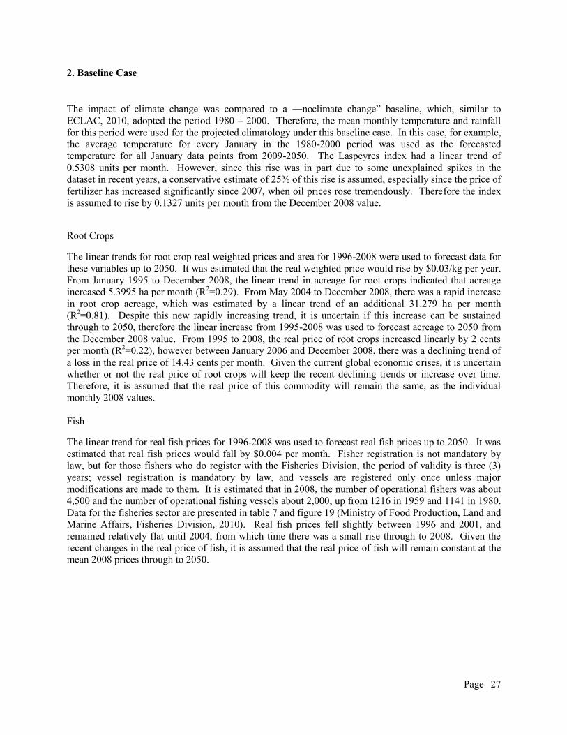
2. Baseline Case

The impact of climate change was compared to a ―no climate change‖ baseline, which, similar to ECLAC, 2010, adopted the period 1980 – 2000. Therefore, the mean monthly temperature and rainfall for this period were used for the projected climatology under this baseline case. In this case, for example, the average temperature for every January in the 1980-2000 period was used as the forecasted temperature for all January data points from 2009-2050. The Laspeyres index had a linear trend of 0.5308 units per month. However, since this rise was in part due to some unexplained spikes in the dataset in recent years, a conservative estimate of 25% of this rise is assumed, especially since the price of fertilizer has increased significantly since 2007, when oil prices rose tremendously. Therefore the index is assumed to rise by 0.1327 units per month from the December 2008 value.

Root Crops

The linear trends for root crop real weighted prices and area for 1996-2008 were used to forecast data for these variables up to 2050. It was estimated that the real weighted price would rise by $0.03/kg per year. From January 1995 to December 2008, the linear trend in acreage for root crops indicated that acreage increased 5.3995 ha per month (R2=0.29). From May 2004 to December 2008, there was a rapid increase in root crop acreage, which was estimated by a linear trend of an additional 31.279 ha per month (R2=0.81). Despite this new rapidly increasing trend, it is uncertain if this increase can be sustained through to 2050, therefore the linear increase from 1995-2008 was used to forecast acreage to 2050 from the December 2008 value. From 1995 to 2008, the real price of root crops increased linearly by 2 cents per month (R2=0.22), however between January 2006 and December 2008, there was a declining trend of a loss in the real price of 14.43 cents per month. Given the current global economic crises, it is uncertain whether or not the real price of root crops will keep the recent declining trends or increase over time. Therefore, it is assumed that the real price of this commodity will remain the same, as the individual monthly 2008 values. Fish

The linear trend for real fish prices for 1996-2008 was used to forecast real fish prices up to 2050. It was estimated that real fish prices would fall by $0.004 per month. Fisher registration is not mandatory by law, but for those fishers who do register with the Fisheries Division, the period of validity is three (3) years; vessel registration is mandatory by law, and vessels are registered only once unless major modifications are made to them. It is estimated that in 2008, the number of operational fishers was about 4,500 and the number of operational fishing vessels about 2,000, up from 1216 in 1959 and 1141 in 1980. Data for the fisheries sector are presented in table 7 and figure 19 (Ministry of Food Production, Land and Marine Affairs, Fisheries Division, 2010). Real fish prices fell slightly between 1996 and 2001, and remained relatively flat until 2004, from which time there was a small rise through to 2008. Given the recent changes in the real price of fish, it is assumed that the real price of fish will remain constant at the mean 2008 prices through to 2050.

Page | 28

Table 7: Estimated Total Annual Value (Millions TT$) of Fish Landings for Trinidad from 2001-2008

Fleet 2001 2002 2003 2004 2005 2006 2007 2008 Artisanal Multi-Gear (Nets & Lines)

105.17 112.72 79.02 96.48 125.04 90.34 94.02 112.58

Artisanal Trawl 10.70 8.25 6.96 6.89 10.73 9.23 7.32 8.03 Semi-Industrial Trawl 4.93 4.54 4.17 3.04 4.59 4.27 4.17 3.88 Industrial Trawl 13.14 15.98 11.25 10.38 14.11 18.35 20.04 21.83 Semi-Industrial Longline 4.50 9.68 11.24 12.69 15.95 20.94 Semi-Industrial Fishpot / A La Vive

15.60 15.60 15.60 15.60 15.60 15.60 15.60 15.60

Total 154.05 166.75 128.24 145.08 186.02 158.72 N/A N/A

Figure 19: Monthly Trips, 1996 – 2008 (a), and Nominal and Real Fish Prices (b)

Green Vegetables

From January 1995 to December 2008, the linear trend in acreage for root crops indicated that acreage increased 5.3995 ha per month (R2=0.29). From June 1995 to December 2008, the increase in vegetable acreage was estimated by a linear trend of an additional 8.7 ha per month. Despite this new rapidly increasing trend, it is uncertain if this increase can be sustained through to 2050, therefore it was assumed that area would increase at 25% of this rate. From 1995 to 2008, the real price of vegetables increased linearly by 2.7 cents per month (R2=0.30), however between 1995 and 2003, these prices were relatively stable at about $4/kg, then rose rapidly to a peak of $15.15 in May 2007, and has been declining subsequently, and reached $4.90 in December 2008. Given the current global economic crises, it is uncertain whether or not the real price of vegetables will keep the recent declining trend or increase over time. Therefore, it is assumed that the real price of this commodity will remain the same, as the individual monthly 2008 values.

Based on the annual trend for temperature from 1970-2008, the estimated linear trend was

applied to the monthly data, and projected to 2050. Here, it was calculated that temperature would increase by 0.007 C per bimonthly period. The same procedure was applied to forecasting rainfall for the baseline, which yielded an estimate of a fall in mean monthly rainfall by 0.0075 mm per bimonthly period. The long run linear trend (1970-2008) was used to avoid

Page | 29

biases in the movement of temperature and rainfall in the short run (1995-2008). The linear trend for green vegetable real weighted prices area for 1995-2008 was determined to be an increase of $0.05 per bi-monthly period. For a more conservative estimate, it was assumed that the future trend would be half of this slope ($0.03). Based on this forecasts of the real price was calculated up to 2050. Fertilizer imports were estimated to rise linearly by 1,234.9 kg per month between 1995 and 2008, therefore this rate was used to project the future changes in this variable.

3. A2 and B2 Scenarios In each of these scenarios, the same assumptions for the behaviour of the non-climate variables in the baseline case into the forecast period were made, except for temperature and precipitation where the forecasted A2 and B2 values (based on the PRECIS ECHAM model) were utilized. Graphical forecasts of rainfall and temperature to 2050 are shown in figures 20 and 21. For the A2 scenario, rainfall is expected to fall slightly through to 2020 (see table 8), and fall by approximately 10% relative to the baseline case in the 2020s, but is expected to rise thereafter, until by the 2040s rainfall rises slightly above the mean for the baseline case. For B2, rainfall rose slightly above the mean for the baseline case in the current decade, but falls steadily thereafter to approximately 15% by the 2040s. Over the same period, temperature is expected to increase by 1.34 C and 1.37 C under A2 and B2 respectively. The projected intra-year variations, relative to the baseline case, are shown in tables 9 and 10.

Figure 20: Historical and Projected Mean Monthly Rainfall – Trinidad & Tobago for the A2 and

B2 Scenarios

Source: Author‘s compilation

Page | 30

Figure 21: Historical and Projected Mean Monthly Temperature – Trinidad & Tobago for the A2

and B2 Scenarios


Table 8: Historical and Projected Mean Monthly Temperature and Rainfall – Trinidad & Tobago for the A2 and B2 Scenarios

2011-2020 2021-2030 2031-2040 2041-2050 A2 B2 A2 B2 A2 B2 A2 B2 Mean Temperature (1980-2000) = 27.08°C Temp (°C ) 27.66 27.54 27.86 27.96 28.08 28.14 28.42 28.45 Temp (D°C ) 0.58 0.46 0.78 0.88 1.00 1.06 1.34 1.37 Mean Rainfall (1980-2000) = 165.97 mm Rain (mm) 160.41 170.27 148.23 153.27 162.80 142.50 170.81 140.78 Rain (%D) -3.35 2.59 -10.69 -7.65 -1.91 -14.14 2.92 -15.18


Table 9: Historical and Projected Mean Monthly Temperature – Trinidad & Tobago for the A2 and B2 Scenarios, by Season

2011-2020 2021-2030 2031-2040 2041-2050 A2 B2 A2 B2 A2 B2 A2 B2 Mean Temperature (1980-2000) = 26.86°C Dry Temp (°C ) 27.47 27.28 27.66 27.68 27.80 27.86 28.15 28.17 Temp ( °C ) 0.61 0.42 0.80 0.82 0.94 1.00 1.29 1.31 Wet Mean Temperature (1980-2000) = 27.24°C Temp (°C ) 27.92 27.82 28.05 28.25 28.37 28.42 28.73 28.73 Temp ( °C ) 0.68 0.58 0.81 1.01 1.13 1.18 1.49 1.49


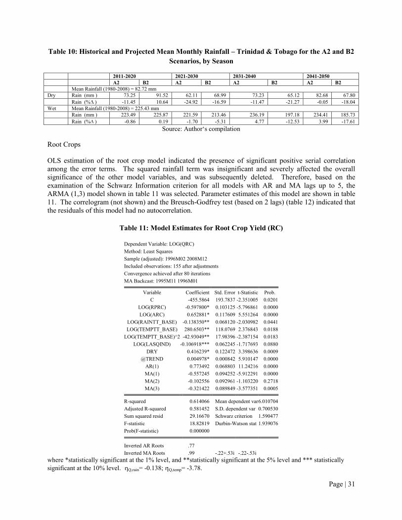
Page | 31

Table 10: Historical and Projected Mean Monthly Rainfall – Trinidad & Tobago for the A2 and B2 Scenarios, by Season

2011-2020 2021-2030 2031-2040 2041-2050 A2 B2 A2 B2 A2 B2 A2 B2 Mean Rainfall (1980-2008) = 82.72 mm Dry Rain (mm ) 73.25 91.52 62.11 68.99 73.23 65.12 82.68 67.80 Rain (% ) -11.45 10.64 -24.92 -16.59 -11.47 -21.27 -0.05 -18.04 Wet Mean Rainfall (1980-2008) = 225.43 mm Rain (mm ) 223.49 225.87 221.59 213.46 236.19 197.18 234.41 185.73 Rain (% ) -0.86 0.19 -1.70 -5.31 4.77 -12.53 3.99 -17.61


Root Crops

OLS estimation of the root crop model indicated the presence of significant positive serial correlation among the error terms. The squared rainfall term was insignificant and severely affected the overall significance of the other model variables, and was subsequently deleted. Therefore, based on the examination of the Schwarz Information criterion for all models with AR and MA lags up to 5, the ARMA (1,3) model shown in table 11 was selected. Parameter estimates of this model are shown in table 11. The correlogram (not shown) and the Breusch-Godfrey test (based on 2 lags) (table 12) indicated that the residuals of this model had no autocorrelation.

Table 11: Model Estimates for Root Crop Yield (RC)

Dependent Variable: LOG(QRC) Method: Least Squares Sample (adjusted): 1996M02 2008M12 Included observations: 155 after adjustments Convergence achieved after 80 iterations MA Backcast: 1995M11 1996M01

Variable Coefficient Std. Error t-Statistic Prob.

C -455.5864 193.7837 -2.351005 0.0201 LOG(RPRC) -0.597800* 0.103125 -5.796861 0.0000 LOG(ARC) 0.652881* 0.117609 5.551264 0.0000

LOG(RAINTT_BASE) -0.138350** 0.068120 -2.030982 0.0441 LOG(TEMPTT_BASE) 280.6503** 118.0769 2.376843 0.0188

LOG(TEMPTT_BASE)^2 -42.93049** 17.98396 -2.387154 0.0183 LOG(LASQIND) -0.106918*** 0.062245 -1.717693 0.0880

DRY 0.416239* 0.122472 3.398636 0.0009 @TREND 0.004978* 0.000842 5.910147 0.0000

AR(1) 0.773492 0.068803 11.24216 0.0000 MA(1) -0.557245 0.094252 -5.912291 0.0000 MA(2) -0.102556 0.092961 -1.103220 0.2718 MA(3) -0.321422 0.089849 -3.577351 0.0005

R-squared 0.614066 Mean dependent var 6.010704 Adjusted R-squared 0.581452 S.D. dependent var 0.700530 Sum squared resid 29.16670 Schwarz criterion 1.590477 F-statistic 18.82819 Durbin-Watson stat 1.939076 Prob(F-statistic) 0.000000

Inverted AR Roots .77

Inverted MA Roots .99 -.22+.53i -.22-.53i where *statistically significant at the 1% level, and **statistically significant at the 5% level and *** statistically significant at the 10% level. Q,rain= -0.138; Q,temp= -3.78.

Page | 32

All the key explanatory variables were significant. Given the mean monthly rainfall of 166.5 mm

from 1995 to 2008, the mean annual rainfall is 1998 mm. This value exceeds the optimal rainfall range for cassava, yam and sweet potatoes, and is at the upper end of the optimal range for dasheen, tannia and eddoes (see Appendix 2). Therefore it is expected that any further increase in rainfall should have a deleterious effect on root crop production as a whole, since the above mentioned crops represent the majority of root crops included in the study. Therefore, the computed elasticities of output for rainfall had the expected sign, also given that most of the root crop production occurs in the dry season. In addition, with the exception of ginger, the upper temperature limit for the root crops included in the study was 30 C. Given that the mean temperature from 1995 to 2008 was 27.08 C, further expected increases in temperature will result in the ambient temperature being very close to the optimal end of the range for most of these crops. Therefore the sign for temperature was as expected.

The signs on all the other variables were as expected, except for real price and the Laspeyres Index. The model results indicated that a 1% increase in real vegetable prices would lead to a 0.60% decrease in harvests, whereas a 1% increase in area would lead to a 0.65% increase in harvests. A 1% increase in rainfall is expected to cause an approximate 0.14% decrease in root crop harvests. Therefore, the anticipated fall in rainfall is expected to have a positive impact on root crop production.

Table 12: Breusch-Godfrey Serial Correlation LM Test for the Root Crops Model

F-statistic 1.162137 Prob. F(2,140) 0.3158

Obs*R-squared 2.288380 Prob. Chi-Square(2) 0.3185

Tests of the stationarity of all model variables (logged) were done (see table 13). The tests conducted were: the Augmented Dickey-Fuller (ADF) test, the Phillips-Perron (PP) test and the Kwiatkowski, Phillips, Schmidt, and Shin (KPSS) Unit Root test. Based on these, none of the model variables were found to be non-stationary.

Table 13: Results of Unit Root tests for logged model variables

Variable Unit Root Tests Unit Root1 ADF (Probability Values) PP (Probability Values) KPSS (LM-Stat)2 Lasqind 0.0000 0.0000 0.6537 No Rain 0.0000 0.0000 0.0838 No Temp 0.0001 0.0001 0.2989 No Qrc 0.0000 0.0000 0.6785 No Rprc 0.0002 0.0003 0.6495 No Arc 0.0195 0.0207 0.7018 No 1 Assumed an intercept in the test equation. 2 Critical values = [1%, 0.7390; 5%, 0.4630; 10%, 0.3470]

Forecasts of root crop harvest under the baseline case are shown in figure 22. While there is only a gradual rise in harvests over time, the confidence bands on these forecasts while initially narrow, widen greatly over time, indicating that the model forecasts are not very robust further in the future, but may be used with a fair degree of confidence in the next 2 decades.

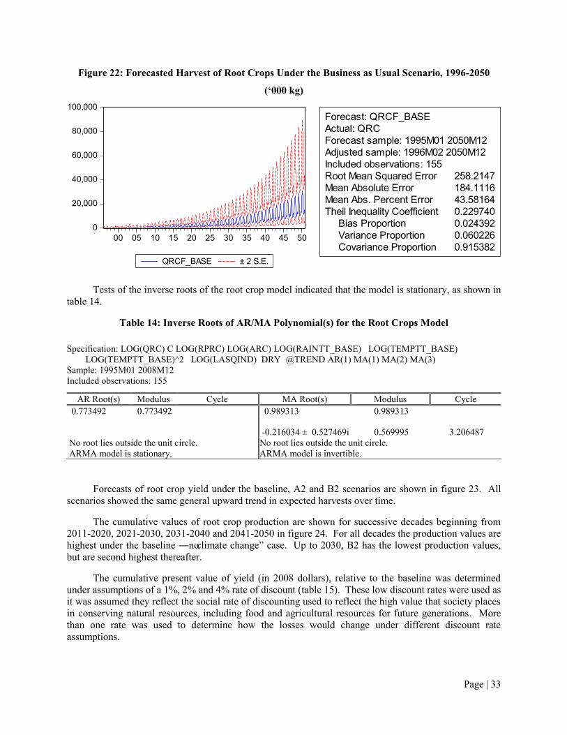
Page | 33

Figure 22: Forecasted Harvest of Root Crops Under the Business as Usual Scenario, 1996-2050

(‘000 kg)

0

20,000

40,000

60,000

80,000

100,000

00 05 10 15 20 25 30 35 40 45 50

QRCF_BASE ± 2 S.E.

Forecast: QRCF_BASEActual: QRCForecast sample: 1995M01 2050M12Adjusted sample: 1996M02 2050M12Included observations: 155Root Mean Squared Error 258.2147Mean Absolute Error 184.1116Mean Abs. Percent Error 43.58164Theil Inequality Coefficient 0.229740 Bias Proportion 0.024392 Variance Proportion 0.060226 Covariance Proportion 0.915382

Tests of the inverse roots of the root crop model indicated that the model is stationary, as shown in table 14.

Table 14: Inverse Roots of AR/MA Polynomial(s) for the Root Crops Model

Specification: LOG(QRC) C LOG(RPRC) LOG(ARC) LOG(RAINTT_BASE) LOG(TEMPTT_BASE) LOG(TEMPTT_BASE)^2 LOG(LASQIND) DRY @TREND AR(1) MA(1) MA(2) MA(3) Sample: 1995M01 2008M12 Included observations: 155

AR Root(s) Modulus Cycle MA Root(s) Modulus Cycle

0.773492 0.773492 0.989313 0.989313

-0.216034 ± 0.527469i 0.569995 3.206487 No root lies outside the unit circle. No root lies outside the unit circle. ARMA model is stationary. ARMA model is invertible.

Forecasts of root crop yield under the baseline, A2 and B2 scenarios are shown in figure 23. All scenarios showed the same general upward trend in expected harvests over time.

The cumulative values of root crop production are shown for successive decades beginning from 2011-2020, 2021-2030, 2031-2040 and 2041-2050 in figure 24. For all decades the production values are highest under the baseline ―no climate change‖ case. Up to 2030, B2 has the lowest production values, but are second highest thereafter.

The cumulative present value of yield (in 2008 dollars), relative to the baseline was determined under assumptions of a 1%, 2% and 4% rate of discount (table 15). These low discount rates were used as it was assumed they reflect the social rate of discounting used to reflect the high value that society places in conserving natural resources, including food and agricultural resources for future generations. More than one rate was used to determine how the losses would change under different discount rate assumptions.

Page | 34

Figure 23: Projections for Root Crop Harvests under the BAU, A2 and B2 Scenarios (‘000 kg)


Figure 24: Cumulative Values of Root Crop Production


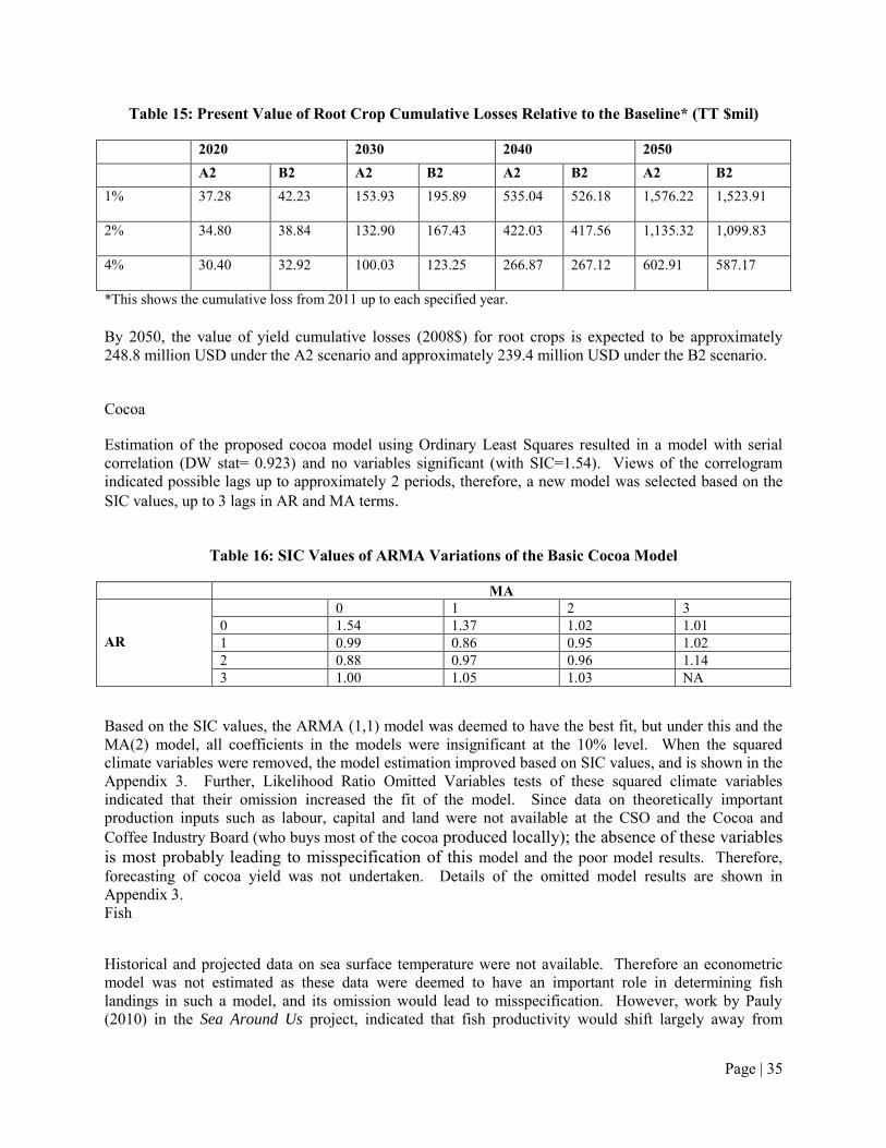
Page | 35

Table 15: Present Value of Root Crop Cumulative Losses Relative to the Baseline* (TT $mil)

2020 2030 2040 2050 A2 B2 A2 B2 A2 B2 A2 B2 1% 37.28 42.23 153.93 195.89 535.04 526.18 1,576.22 1,523.91

2% 34.80 38.84 132.90 167.43 422.03 417.56 1,135.32 1,099.83

4% 30.40 32.92 100.03 123.25 266.87 267.12 602.91 587.17

*This shows the cumulative loss from 2011 up to each specified year. By 2050, the value of yield cumulative losses (2008$) for root crops is expected to be approximately 248.8 million USD under the A2 scenario and approximately 239.4 million USD under the B2 scenario.

Cocoa

Estimation of the proposed cocoa model using Ordinary Least Squares resulted in a model with serial correlation (DW stat= 0.923) and no variables significant (with SIC=1.54). Views of the correlogram indicated possible lags up to approximately 2 periods, therefore, a new model was selected based on the SIC values, up to 3 lags in AR and MA terms.

Table 16: SIC Values of ARMA Variations of the Basic Cocoa Model

MA AR

0 1 2 3 0 1.54 1.37 1.02 1.01 1 0.99 0.86 0.95 1.02 2 0.88 0.97 0.96 1.14 3 1.00 1.05 1.03 NA

Based on the SIC values, the ARMA (1,1) model was deemed to have the best fit, but under this and the MA(2) model, all coefficients in the models were insignificant at the 10% level. When the squared climate variables were removed, the model estimation improved based on SIC values, and is shown in the Appendix 3. Further, Likelihood Ratio Omitted Variables tests of these squared climate variables indicated that their omission increased the fit of the model. Since data on theoretically important production inputs such as labour, capital and land were not available at the CSO and the Cocoa and Coffee Industry Board (who buys most of the cocoa produced locally); the absence of these variables is most probably leading to misspecification of this model and the poor model results. Therefore, forecasting of cocoa yield was not undertaken. Details of the omitted model results are shown in Appendix 3. Fish

Historical and projected data on sea surface temperature were not available. Therefore an econometric model was not estimated as these data were deemed to have an important role in determining fish landings in such a model, and its omission would lead to misspecification. However, work by Pauly (2010) in the Sea Around Us project, indicated that fish productivity would shift largely away from

Page | 36

tropical regions and towards higher latitudes (towards the poles), which would in general have a severe impact in the Caribbean. Utilizing data on the landings of all commercial species worldwide, a temperature preference profile was created for each species, which showed the regions that each species prefers to inhabit based on historical temperatures. Then, on a small scale (each 0.5 degree latitude and longitude), a population dynamics model was formulated to indicate the distribution range of each species, incorporating biological relationships, including the incidence of egg and larvae production, which are also affected by sea temperature.

The model used projections of sea temperature from the Ocean-Atmosphere Coupled General Circulation model (GCM) CM 2.1 of the National Oceanic and Atmospheric Administration (NOAA)‘s Geophysical Fluid Dynamics Laboratory, and also accounted for changes in currents for three GHG emission scenarios: 720 ppm, 550 ppm and 370 ppm CO2 concentration by 2100. The potential catch was then determined based on productivity in the new distribution area for each of the 1066 species in the model. By generating global maps in changes in catch potential (see figure 25), Pauly (2010) estimated that for the Caribbean Large Marine Ecosystem, there will be a decrease in catch potential of 10 - 20% by 2050 relative to 2005 catch potentials, other things remaining constant. Individual country estimates were not presented.

Figure 25: Predicted Changes in Global Catch Potentials

Source: Pauly (2010), figure 3

Given the range in possible reductions by Pauly (2010), and since the A2 scenario is the expected higher impact (higher GHG emission scenario) scenario, it was estimated that under the A2 and B2 scenarios, fisheries revenue loss would be 20% and 10% of the 2005 fish landings revenue, respectively. The 2005 total commercial landings of 15,889 tonnes for Trinidad and Tobago (see Appendix 1) were used as the baseline case for the analysis. The associated ex-vessel value was TT$186.02 mil. The 2005 landings were assumed constant to 2050 in the baseline case, and real prices were fixed during this period at the mean 2008 real price. The real price was also assumed to be fixed under the A2 and B2 scenarios.

The cumulative present value of losses, relative to the baseline was determined under assumptions of a 1%, 2% and 4% rate of discount (see table 17). By 2050 under the A2 and B2 scenarios, losses in real terms were estimated to be 29.3 million USD and $508.6 mil respectively, at a 1% discount rate.

Page | 37

Table 17: Present Value of Cumulative Losses Relative to the Baseline (TT$mil)

2020 2030 2040 2050 A2 B2 A2 B2 A2 B2 A2 B2

1% 126.43 63.21 350.75 175.37 653.28 326.64 1,017.19 508.60 2% 116.65 58.33 304.92 152.46 535.31 267.66 786.61 393.31 4% 99.75 49.88 233.36 116.68 368.36 184.18 489.77 244.89

Green Vegetables

OLS estimation indicated the presence of significant positive serial correlation among the error terms. Therefore, based on the examination of the Schwarz Information criterion for all models with AR and MA lags up to 5, the ARMA (2,2) model shown in table 18 was selected. Parameter estimates of this model are shown below. The correlogram and the Breusch-Godfrey test (table 19) indicated that the residuals of this model had no autocorrelation.

Table 18: Model Estimates for Green Vegetables

Dependent Variable: LOG(QVEG) Method: Least Squares Sample (adjusted): 1995M03 2008M12 Included observations: 166 after adjustments Convergence achieved after 24 iterations MA Backcast: 1995M01 1995M02

Variable Coefficient Std. Error t-Statistic Prob. C 293.5634 140.8741 2.083871 0.0388

LOG(RPVEG) -0.808485* 0.069170 -11.68837 0.0000 LOG(AVEG) 0.272838** 0.129340 2.109456 0.0365

LOG(RAINTT) -0.761402** 0.305511 -2.492223 0.0138 LOG(RAINTT)^2 0.081325** 0.034339 2.368284 0.0191 LOG(TEMPTT) -172.8033** 85.76769 -2.014783 0.0457

LOG(TEMPTT)^2 26.25488** 13.04478 2.012673 0.0459 LOG(FIMQ) -0.061115*** 0.035851 -1.704695 0.0903

AR(1) -0.266578 0.035353 -7.540353 0.0000 AR(2) -0.885227 0.034471 -25.68024 0.0000 MA(1) 0.388798 0.011637 33.41059 0.0000 MA(2) 0.977952 0.007682 127.2994 0.0000

R-squared 0.558108 Mean dependent var 7.461319

Adjusted R-squared 0.526544 S.D. dependent var 0.510850 Sum squared resid 19.02773 Schwarz criterion 1.041328 F-statistic 17.68194 Durbin-Watson stat 1.956242 Prob(F-statistic) 0.000000

Inverted AR Roots -.13+.93i -.13-.93i

Inverted MA Roots -.19-.97i -.19+.97i *statistically significant at the 1% level **statistically significant at the 5% level and ***statistically significant at

the 10% level. Q,rain=0.0706; Q,temp=1.1474

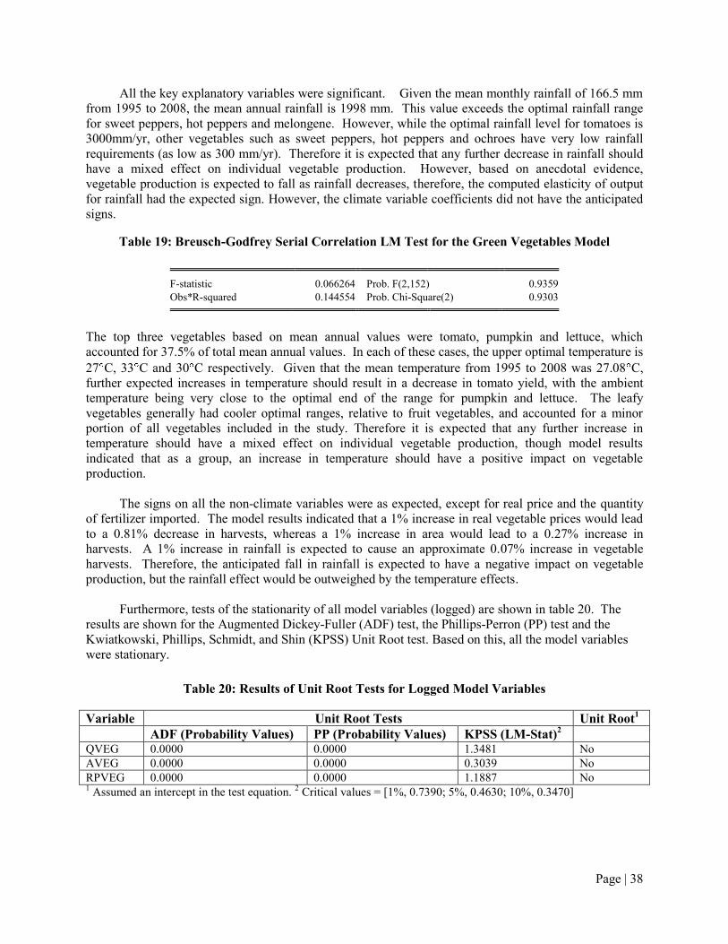
Page | 38

All the key explanatory variables were significant. Given the mean monthly rainfall of 166.5 mm from 1995 to 2008, the mean annual rainfall is 1998 mm. This value exceeds the optimal rainfall range for sweet peppers, hot peppers and melongene. However, while the optimal rainfall level for tomatoes is 3000mm/yr, other vegetables such as sweet peppers, hot peppers and ochroes have very low rainfall requirements (as low as 300 mm/yr). Therefore it is expected that any further decrease in rainfall should have a mixed effect on individual vegetable production. However, based on anecdotal evidence, vegetable production is expected to fall as rainfall decreases, therefore, the computed elasticity of output for rainfall had the expected sign. However, the climate variable coefficients did not have the anticipated signs.

Table 19: Breusch-Godfrey Serial Correlation LM Test for the Green Vegetables Model

F-statistic 0.066264 Prob. F(2,152) 0.9359

Obs*R-squared 0.144554 Prob. Chi-Square(2) 0.9303

The top three vegetables based on mean annual values were tomato, pumpkin and lettuce, which accounted for 37.5% of total mean annual values. In each of these cases, the upper optimal temperature is 27 C, 33 C and 30 C respectively. Given that the mean temperature from 1995 to 2008 was 27.08 C, further expected increases in temperature should result in a decrease in tomato yield, with the ambient temperature being very close to the optimal end of the range for pumpkin and lettuce. The leafy vegetables generally had cooler optimal ranges, relative to fruit vegetables, and accounted for a minor portion of all vegetables included in the study. Therefore it is expected that any further increase in temperature should have a mixed effect on individual vegetable production, though model results indicated that as a group, an increase in temperature should have a positive impact on vegetable production.

The signs on all the non-climate variables were as expected, except for real price and the quantity of fertilizer imported. The model results indicated that a 1% increase in real vegetable prices would lead to a 0.81% decrease in harvests, whereas a 1% increase in area would lead to a 0.27% increase in harvests. A 1% increase in rainfall is expected to cause an approximate 0.07% increase in vegetable harvests. Therefore, the anticipated fall in rainfall is expected to have a negative impact on vegetable production, but the rainfall effect would be outweighed by the temperature effects.

Furthermore, tests of the stationarity of all model variables (logged) are shown in table 20. The results are shown for the Augmented Dickey-Fuller (ADF) test, the Phillips-Perron (PP) test and the Kwiatkowski, Phillips, Schmidt, and Shin (KPSS) Unit Root test. Based on this, all the model variables were stationary.

Table 20: Results of Unit Root Tests for Logged Model Variables

Variable Unit Root Tests Unit Root1 ADF (Probability Values) PP (Probability Values) KPSS (LM-Stat)2 QVEG 0.0000 0.0000 1.3481 No AVEG 0.0000 0.0000 0.3039 No RPVEG 0.0000 0.0000 1.1887 No 1 Assumed an intercept in the test equation. 2 Critical values = [1%, 0.7390; 5%, 0.4630; 10%, 0.3470]

Page | 39

Forecasts of vegetable harvests under the baseline case are shown in figure 26. Yields are expected to rise gradually over the forecast period.

Figure 26: Forecasted Green Vegetable Harvests Under the Business as Usual Scenario, 1996-2050

(‘000 kg)

0

4,000

8,000

12,000

16,000

00 05 10 15 20 25 30 35 40 45 50

QVEGF_BASE ± 2 S.E.

Forecast: QVEGF_BASEActual: QVEGForecast sample: 1995M01 2050M12Adjusted sample: 1995M03 2050M12Included observations: 166Root Mean Squared Error 792.7344Mean Absolute Error 543.6768Mean Abs. Percent Error 29.15370Theil Inequality Coefficient 0.185565 Bias Proportion 0.027622 Variance Proportion 0.315932 Covariance Proportion 0.656446

Tests of the inverse roots of the green vegetable model indicated that the model is stationary, as shown in table 21.

Table 21: Inverse Roots of AR/MA Polynomial(s) for the Green Vegetables Model

Specification: LOG(QVEG) C LOG(RPVEG) LOG(AVEG) LOG(RAINTT) LOG(RAINTT)^2 LOG(TEMPTT) LOG(TEMPTT)^2 AR(1) AR(2) MA(1) MA(2) LOG(FIMQ) Sample: 1995M01 2008M12 Included observations: 166

AR Root(s) Modulus Cycle

-0.133289 ± 0.931376i 0.940865 3.668069

No root lies outside the unit circle. ARMA model is stationary.

MA Root(s) Modulus Cycle

-0.194399 ± 0.969619i 0.988915 3.552505

No root lies outside the unit circle. ARMA model is invertible.

Forecasts for vegetable yield are shown in figure 27. Overall, yield is expected to increase under all scenarios, though the increase is best under the A2 scenario by 1950.

Page | 40

Figure 27: Projections for the Value of Vegetable Yield under the BAU, A2 and B2 Scenarios (‘000

TT$)

The cumulative values of vegetable production are shown for successive decades beginning from 2011-2020, 2021-2030 until 2050 in figure 28 below. For all decades the production values are highest under the A2 scenario, followed by B2 and the baseline case.

Figure 28: Cumulative Values of Root Crop Production

The cumulative present value of yield, relative to the baseline case was determined under assumptions of a 1%, 2% and 4% rate of discount. The values are presented in table 22.

Page | 41

Table 22: Present Value of Cumulative Vegetable Losses Relative to the Baseline (TT $mil)

2020 2030 2040 2050 A2 B2 A2 B2 A2 B2 A2 B2 1% -65.06 -44.61 -146.16 -115.79 -235.30 -214.67 -349.14 -312.32

2% -60.64 -41.31 -128.45 -100.99 -196.37 -176.47 -274.92 -243.75

4% -52.85 -35.53 -100.38 -77.60 -139.92 -121.71 -177.44 -153.76

*This shows the cumulative loss (gains are negative) up to each specified year. Source: Author‘s compilation. By 2050, the value of yield cumulative gains (2008$) for vegetables is expected to be approximately 54.9 million USD under the A2 scenario and approximately 49.1 million USD under the B2 scenario, given a 1% discount rate.

C. AGGREGATE VALUE OF YIELD LOSS FOR ROOT CROPS, FISHERIES AND VEGETABLE PRODUCTION

Relative to the baseline case, the key subsectors in agriculture would be subjected to mixed impacts under the A2 and B2 scenarios. Fisheries outputs are expected to fall with climate change, but root crop and vegetable production are expected to rise. However, relative to the baseline, the values of yield will be worse under the A2 and B2 scenarios for both root crop and fisheries outputs, but better under these two scenarios for vegetable production, since most of the key vegetables have a relatively high temperature range for optimal production. In aggregate, in every decade up to 2050, these three key sub-sectors combined are expected to experience a loss under climate change, all scenarios, with the highest losses under A2. By 2050, the cumulative loss under A2 is calculated as approximately 352.8 million USD and approximately 270.8 million USD under B2 (table 23). These values as a percentage of the 2008 nominal GDP are shown in table 24.

Table 23: Present Value of Cumulative Losses for Agricultural Yield Relative to the Baseline (TT $mil)

2020 2030 2040 2050 A2 B2 A2 B2 A2 B2 A2 B2 1% 98.66 60.83 358.52 255.48 953.02 638.16 2,244.27 1,720.19

2% 90.81 55.85 309.37 218.90 760.97 508.74 1,647.02 1,249.39

4% 77.31 47.26 233.00 162.33 495.31 329.59 915.25 678.30


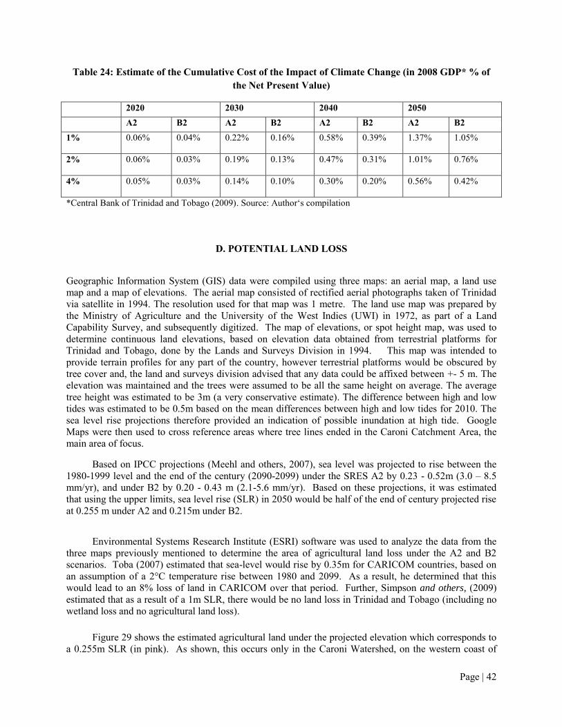
Page | 42

Table 24: Estimate of the Cumulative Cost of the Impact of Climate Change (in 2008 GDP* % of the Net Present Value)

2020 2030 2040 2050 A2 B2 A2 B2 A2 B2 A2 B2 1% 0.06% 0.04% 0.22% 0.16% 0.58% 0.39% 1.37% 1.05%

2% 0.06% 0.03% 0.19% 0.13% 0.47% 0.31% 1.01% 0.76%

4% 0.05% 0.03% 0.14% 0.10% 0.30% 0.20% 0.56% 0.42%

*Central Bank of Trinidad and Tobago (2009). Source: Author‘s compilation

D. POTENTIAL LAND LOSS

Geographic Information System (GIS) data were compiled using three maps: an aerial map, a land use map and a map of elevations. The aerial map consisted of rectified aerial photographs taken of Trinidad via satellite in 1994. The resolution used for that map was 1 metre. The land use map was prepared by the Ministry of Agriculture and the University of the West Indies (UWI) in 1972, as part of a Land Capability Survey, and subsequently digitized. The map of elevations, or spot height map, was used to determine continuous land elevations, based on elevation data obtained from terrestrial platforms for Trinidad and Tobago, done by the Lands and Surveys Division in 1994. This map was intended to provide terrain profiles for any part of the country, however terrestrial platforms would be obscured by tree cover and, the land and surveys division advised that any data could be affixed between +- 5 m. The elevation was maintained and the trees were assumed to be all the same height on average. The average tree height was estimated to be 3m (a very conservative estimate). The difference between high and low tides was estimated to be 0.5m based on the mean differences between high and low tides for 2010. The sea level rise projections therefore provided an indication of possible inundation at high tide. Google Maps were then used to cross reference areas where tree lines ended in the Caroni Catchment Area, the main area of focus.

Based on IPCC projections (Meehl and others, 2007), sea level was projected to rise between the 1980-1999 level and the end of the century (2090-2099) under the SRES A2 by 0.23 - 0.52m (3.0 – 8.5 mm/yr), and under B2 by 0.20 - 0.43 m (2.1-5.6 mm/yr). Based on these projections, it was estimated that using the upper limits, sea level rise (SLR) in 2050 would be half of the end of century projected rise at 0.255 m under A2 and 0.215m under B2.

Environmental Systems Research Institute (ESRI) software was used to analyze the data from the three maps previously mentioned to determine the area of agricultural land loss under the A2 and B2 scenarios. Toba (2007) estimated that sea-level would rise by 0.35m for CARICOM countries, based on an assumption of a 2°C temperature rise between 1980 and 2099. As a result, he determined that this would lead to an 8% loss of land in CARICOM over that period. Further, Simpson and others, (2009) estimated that as a result of a 1m SLR, there would be no land loss in Trinidad and Tobago (including no wetland loss and no agricultural land loss).

Figure 29 shows the estimated agricultural land under the projected elevation which corresponds to a 0.255m SLR (in pink). As shown, this occurs only in the Caroni Watershed, on the western coast of

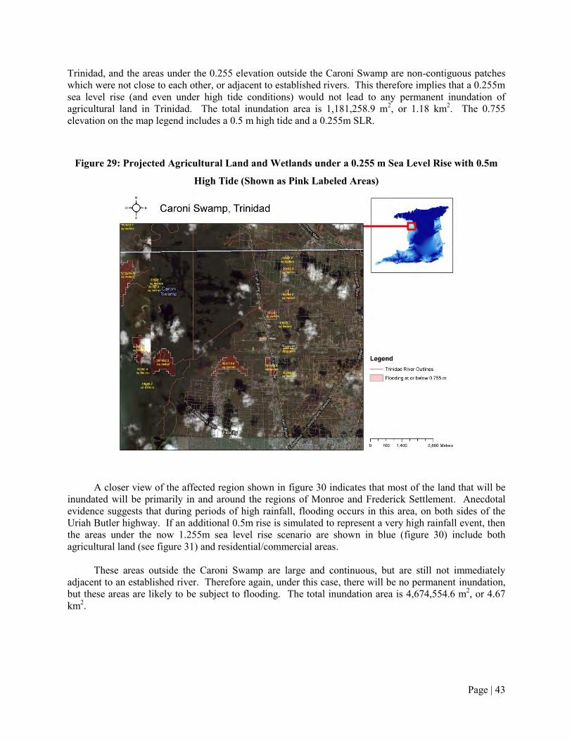
Page | 43

Trinidad, and the areas under the 0.255 elevation outside the Caroni Swamp are non-contiguous patches which were not close to each other, or adjacent to established rivers. This therefore implies that a 0.255m sea level rise (and even under high tide conditions) would not lead to any permanent inundation of agricultural land in Trinidad. The total inundation area is 1,181,258.9 m2, or 1.18 km2. The 0.755 elevation on the map legend includes a 0.5 m high tide and a 0.255m SLR.

Figure 29: Projected Agricultural Land and Wetlands under a 0.255 m Sea Level Rise with 0.5m

High Tide (Shown as Pink Labeled Areas)

A closer view of the affected region shown in figure 30 indicates that most of the land that will be

inundated will be primarily in and around the regions of Monroe and Frederick Settlement. Anecdotal evidence suggests that during periods of high rainfall, flooding occurs in this area, on both sides of the Uriah Butler highway. If an additional 0.5m rise is simulated to represent a very high rainfall event, then the areas under the now 1.255m sea level rise scenario are shown in blue (figure 30) include both agricultural land (see figure 31) and residential/commercial areas.

These areas outside the Caroni Swamp are large and continuous, but are still not immediately adjacent to an established river. Therefore again, under this case, there will be no permanent inundation, but these areas are likely to be subject to flooding. The total inundation area is 4,674,554.6 m2, or 4.67 km2.

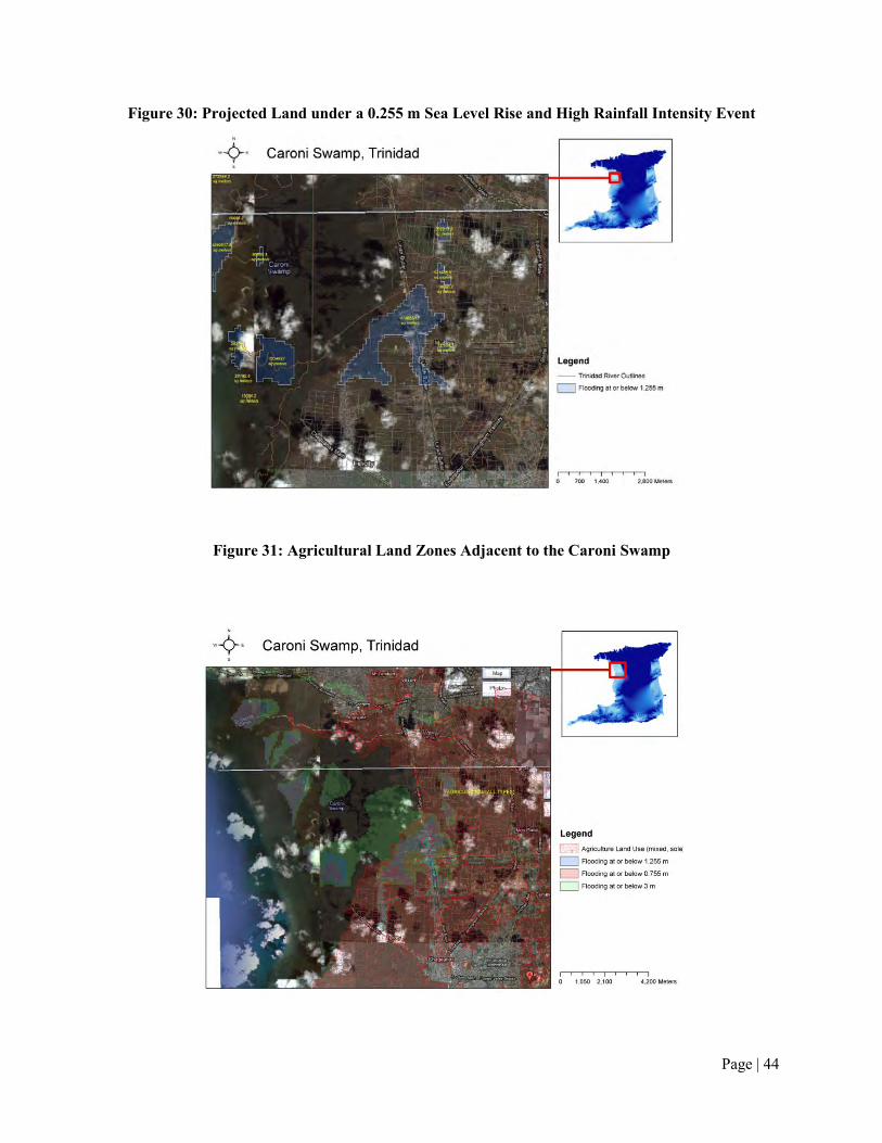
Page | 44

Figure 30: Projected Land under a 0.255 m Sea Level Rise and High Rainfall Intensity Event

Figure 31: Agricultural Land Zones Adjacent to the Caroni Swamp

Page | 45

Most of the areas which are prone to flooding, regardless of the scenario, will be in Class IV soils, which are just east of the Caroni Swamp. Currently, paw-paw, sweet peppers and other vegetables are cultivated extensively in this region, and there are areas in this vicinity that are already flooded due to high tides. Based on Hardy (1977), the soils to the east of the swamp are sub-class IVw soils, on which cultivation is limited by adverse water relations. Soils of this group usually occur on A and B-slopes, and are affected by excessive wetness for longer periods of time. They are all heavy clay soils and occur on alluvial plains which are subject to periodic flooding. Their internal drainage is restricted mainly because of their level land relief and clayey texture. Representatives of this group are Bejucal, Cacandee and Frederick. These clayey soil-series are suitable for the growing of rice in the wet season and market garden crops in the dry season and give only one crop of vegetables that are planted when the soil has partially dried out (under rain-fed conditions). The chief requirement of these soils is thorough drainage.

IV. ADAPTATION OPTIONS AND BENEFIT COST ANALYSES

Some priorities for adaptation in the agricultural sector in Trinidad and Tobago have been identified by the Ministry of the Environment in the Climate Policy, and as articulated by the Ministry of Food Production, Land and Marine Resources. However, this study expanded on the proposed recommendations and ranks each adaptation option from high (score of 5) to low (score of 1) based on internationally proposed criteria for adaptation strategies. The final rank of each proposal was based on resource availability and the policy environment currently in Trinidad and Tobago, and recognized existing adaptation activities or proposals that are currently being planned by the Ministry of Food Production. The rankings are shown in Appendix 4.

Each of the criteria used had the same weight. Based on the eleven (11) evaluation criteria presented in table 27, the top ten (10) potential adaptation options were identified:

1. Use of water saving irrigation systems and water management systems e.g. drip irrigation. 2. Mainstream climate change issues into agricultural management. 3. Repair/maintain existing dams. 4. Alter crop calendar for short-term crops. 5. Adopt improved technologies for soil conservation. 6. Establish systems of food storage. 7. Promote water conservation – install on-farm water harvesting off roof tops. 8. Design and implement holistic water management plans for all competing uses. 9. Build on- farm water storage such as ponds and tanks) (selected from among proposals with the

same rank) 10. Agricultural Drainage. (selected from among proposals with the same rank)

In addition, the following option was evaluated based on promotion of protected agriculture locally:

11. Installation of Greenhouses.

All of these adaptation options are important, but the options which focus on conserving and using water more efficiently are particularly important given that rainfall levels are expected to decline for Trinidad and Tobago through to 2050. The increased temperature is expected to exacerbate heat stress in plants, especially when coupled with a decline in precipitation, so water conservation techniques such as mulching (which conserves both soil and water) are particularly relevant in adapting to climate change. The installation of protected agriculture, such as green houses has received increased attention locally, but is not suitable for root crop production, and may be more useful for vegetable production as temperatures continue to increase past the anticipated levels for 2050.

Page | 46

Establishing the benefits and costs associated with altering the crop calendar was not feasible given the wide variety of crops included in the study. Therefore, a Benefit Cost Analysis (BCA) was not conducted for this option. Therefore, 10 options were used to calculate the Benefit/Cost of each proposal.

Given all the costs and benefits for all adaptation options which were provided in the subsequent section, from 2012 to 2050, the present value of each option was calculated using a 4% discount rate and shown in table 25. It indicates that the most attractive adaptation options, based on the Benefit-Cost Ratio are: (1) Build on- farm water storage such as ponds and tanks (2) Mainstreaming climate change issues into agricultural management and (3) Water harvesting. However, the options with the highest net benefits are, (in order of priority): (1) Build on- farm water storage such as ponds and tanks), (2) Mainstreaming climate change issues into agricultural management and (3) Use of drip irrigation. It should be noted that under the two criteria, different options are proposed. The final choice by governments should include these assessments, as well as the omitted intangible benefits, as well as the provision of other social goals such as employment.

Page | 47

Table 25: Summary of the Present Value Costs and Benefits of the Highest-Ranked Proposed Adaptation Actions for Trinidad and Tobago (4% Discount Rate)

TT$ Details Cumulative Present

Value of Benefits Cumulative Present

Value of Costs Benefit Cost Ratio Net Benefits

Payback Period (years)

Option 1

Use water saving irrigation systems and water management systems e.g. drip irrigation $7,573,792,616.81 $593,733,060.07 12.8 $6,980,059,556.74 0.64

Option 2

Mainstream climate change issues into agricultural management $28,521,600,000.00 $167,322,990.86 170.5 $28,354,277,009.14 0.01

Option 3 Repair/maintain existing dams $67,872,330.00 $25,961,538.46 2.6 $41,910,791.54 0.18

Option 4

Adopt improved technologies for soil conservation $341,830,575.59 $124,265,115.06 2.8 $217,565,460.53 0.00

Option 5 Establish systems of food storage $236,544,000.00 $15,777,944.63 15.0 $220,766,055.37 0.00

Option 6 Water conservation - Water Harvesting $3,029,517,046.72 $34,207,179.97 88.6 $2,995,309,866.76 0.18

Option 7 Water Management Plans $58,777,847.05 $1,201,845.58 48.9 $57,576,001.48 0.06

Option 8

Build on- farm water storage (ponds, tanks etc) $121,235,161,199.09 $150,123,684.47 807.6 $121,085,037,514.62 1.96

Option 9 Agricultural Drainage $210,217,987.50 $233,344,848.39 0.9 ($23,126,860.89) 0.00

Option 10 Installation of Greenhouses $20,387,207.01 $20,387,207.01 1.0 $0.00 0.28

Page | 59

Assumptions Made in Calculating the Costs and Benefits of Adaptation Options

The analysis was done for the period 2012 – 2050.

Option 1: Use Water Saving Irrigation Systems and Water Management Systems e.g. Drip

Irrigation.

It was assumed that: There was transformation of 2% or 219.94 ac of the 2008 green vegetable acreage

from a rain-fed system to a drip irrigation system (Porter's Agri-Industrial Agencies Ltd 2011), each year for 20 yrs.

For the drip irrigation system, the investment cost per acre = $50709. Year 1= 2012. The replacement of drip lines occurs every 5 yrs. The revenue of green vegetables in 2008 was $90,496,440. Irrigation of green vegetables increases yield by 20%. Rate of inflation = 4%.

Option 2: Mainstream Climate Change Issues into Agricultural Management.

It was assumed that: Mainstreaming requires the review of all national policies and projects to ensure that

climate change issues are included. In order to undertake the review, training of 150 workers per year @$5000/person

(in-house training, conferences, travel of experts, study abroad etc) would be needed. An Annual Policy Review utilizes 50 persons. The salary of an Economist I = $8,614.00 (Brathwaite 2011) There is a 2% annual rise in salaries The 2008 nominal GDP is mil TT$ 152,115.20 (Central Bank of Trinidad and

Tobago 2007)

Option 3: Repair/Maintain Existing Dams.

It was assumed that: Rehabilitation of a 0.227 img reservoir costs $1,800,000 (Trinidad and Tobago

WASA 2007). One (1) reservoir is repaired each yr for 5 yrs. The total 2008 green vegetables revenue was $90,496,440. The repairs to dams increase green vegetables revenue by 2%.

Page | 60

Option 4: Adopt Improved Technologies for Soil Conservation.

It was assumed that: Total acreage under green vegetables plus root crops in 2008 = 15,800.66 ac. One (1) roll of polyethylene mulching sheet = TT$2212.89+Vat (an area of 4000ft by

4ft). The plastic mulch is applied to 2% of the acreage of crops per year (316 ac). The mulch application increased yield by 2% on 316 acres. There is a 90% reduction in the labour cost of weeding as a result of applying the

mulch (CARDI 2009) There is an avoided cost for weedicide (except pre-emergent weedicide), labour,

material and equipment cost for insecticide in tomato production (Adams and others

2007).

Option 5: Establish Systems of Food Storage.

It was assumed that: Storage would provide food for 315,392 meals at 1 lb per meal, in the event of a

national emergency. Food storage consists of dry/canned goods and grains such as rice and wheat flour. The products stored are bought as a fiscal incentive and are owned by private firms,

except in national emergencies, when ownership reverts to the State. No replacement is needed for silos in the project period. Four (4) silos to be installed. The details of the cost are shown in table 26.

Table 26: Breakdown of Food Storage Costs

Item Cost(TT$) Reference Ten (10) ton wheat silo @Aus$5830 37778.4 Moylan Grain Silos (2011) Shipping & handling 37778.4 Sub-total 75556.8 Installation - labour 60000 15 persons @$400/day*10 days Total 135556.8 Four (4) warehouses (each of 25 by 40 ft) with holding capacity for143360 kg 6.4 kg food per sq ft 8 ft high stack 70% warehouse capacity Wheat price TT$/metric tonne 1959.552 IndexMundi Rice price TT$/metric tonne 3468.1608 IndexMundi Emergency meals: 315392 1 lb food per meal

Page | 61

Option 6: Promote Water Conservation – Installation of on-Farm Water Harvesting off Roof

Tops.

It was assumed that: Water can be collected off the roofs of on-farm sheds or buildings. The length of each on-farm shed/storage unit is 20ft. Two 1000 gallon tanks @ $2153.00 each + spouts and brackets = TT$3545.6. Benefit of water harvesting is 40% of the benefit of drip irrigation per acre. Labour costs = TT$400/man day. For 2 tanks, 10 ft down spouting and 10 brackets on the downspouts are required. There were 13,874 holdings of crops in 2004 (2004 Census). There is the establishment of 2% of holdings (110) per year with water harvesting

technology.

Option 7: Design and Implement Holistic Water Management Plans for all Competing Uses.

It was assumed that: The design and implementation of an appropriate plan would result in an

improvement in yield of 2% of the 2008 green vegetables and root crop values. Implementation requires 4 persons over 9 months. Follow up requires 2 persons for 6 months. There is a need for four (4) stakeholder consultations at a cost of TT$6000 each. Administration costs include: marketing, office supplies, travel costs, office

equipment and services. The policy review and monitoring occurs every 5 yrs. Follow up administration costs = 20% of Yr1 costs. Persons at a rank of Economist 1 would be employed to undertake the policy writing,

at a salary ofTT$10,000/mth.

Option 8: Build on- Farm Water Storage (Ponds, Tanks Etc)

It was assumed that: Impoundments are dug into the ground on-farm to collect surface runoff. The duration of job to dig a pond lasts 5 days. Excavator cost = $2000/day. Truck to move soil = $1200/day. Track Bobcat = $1800/day. Mobilization of the equipment = $2000/piece to and from the job site. The prices quoted include labour to operate the equipment. Other reference for the construction cost: In Ecuador, the average cost to construct an on-

farm pond was estimated at $0.93/m3 of water, but the range was from $0.10 to $2.00/m3. (Unit of Sustainable Development and Environment General Secretariat 2011). The

Page | 62

operation and maintenance costs ranged between $0.01 and $0.03/m3 of storage capacity. Even using the upper level of cost, these costs are too low for the Caribbean.

The on-farm ponds are established on 1% of crop holdings (138) per year for 10 years. The avoided crop losses = 40% of revenue on 138 farms (2008 value of green vegetables

and root crops). Revenue for vegetables and root crops in 2008($) = $112,116,260.

Option 9: Agricultural Drainage.

It was assumed that: Lumped Capital each year in the project period 10% annual operational cost Benefit = avoided loss to 5% of 2008 green vegetables and root crop values

Option 10: Installation of Greenhouses.

Assumptions of costs and benefits are provided in table 27.

Table 27: Greenhouse Installation Costs

Item Cost Reference Greenhouse Brand - 1 Southern Start Package (EC$) 114,767 Greenhouse Megastore S&H (20%) 22,953 30' by 48' (20 lb rating, 6 ft sidewall) Taxes (15%) 17,215 Land Prep - labour &machinery 5,000 Labour - Installation 32,000 Benches, Drip irrigation 11476.728 Total 203,413 Construct 5 per year for 10 years Traditional yield (tomatoes) 2363.32 Vital Earth Resources (1999) Additional% yield 0.6 Crops/yr 5 Additional yield 7089.96 Price/kg (2008) 9.06

Page | 63

VI. CONSIDERATIONS FOR MITIGATION OPTIONS

A. EMISSIONS

Trinidad and Tobago is a high per-capita emitter of CO2 (figure 32), and experienced 2-fold growth in carbon dioxide emission per capita from 1990 to 2006 (table 28).

Figure 32: Per-Capita CO2 Emissions for Selected Caribbean Countries, 2006

Source: UN Statistical Division

Table 28: CO2 Emissions in 2006

CO2 Emissions

% Change Since 1990

CO2 Emissions Per Capita

CO2 Emissions Per km2

mio. tonnes

% tonnes tonnes Saint Lucia 0.38 130.9 2.34 706.86 St. Vincent and the

Grenadines 0.20 145.5 1.65 509.00

Trinidad and Tobago 33.60 98.1 25.29 6 549.90

United Kingdom 557.86 -5.5 9.20 2 296.64 United States 5975.10 18.1 19.70 620.53

Source: UN Statistics Division.

Page | 64

Even though Trinidad and Tobago‘s contribution to total GHG emissions is less than 1%, its per-

capita rate of emission is very high, so measures to mitigate emissions should be adoption. The main proposals to reduce GHG emissions on the farm are:

Increased use of on-farm renewable energy Reduced use of energy-intensive inputs e.g. fertilizers Generation of fuels on-farm e.g biogas digesters from livestock production Use of more energy efficient heating and lighting

These measures are not appraised economically in this report, however, Trinidad and Tobago should also consider one of the main off-farm sources of mitigation, which has a direct impact on the agricultural sector – reforestation. This issue is elaborated below.

B. LAND LOSS DUE TO FOREST FIRES Based on the area burnt in Trinidad and Tobago between 2005 and 2009, the average annual loss due to fires is 1717.3 ha. The details by vegetation type for 2010 are shown in Appendix 4. Based on the IPCC (2000a) 17.6 106 km2 of Tropical Forests store 428 GtC (gigagtonnes of carbon). Therefore, when an average of 17.173 km2 (1717.3 ha) is lost every year to forest fires (table 29), 4.18 GtC is emitted into the atmosphere. Each carbon credit is for 1 kilo ton of sequestered carbon, therefore based on July 2011 carbon credit prices on the EU market (CarbonPositive 2011), carbon credits were at US$17.41. This implies that for the total land lost to forest fires on average each year, the opportunity cost of carbon credit revenue is US$ 72,773,800 (TT$ 471,574,224)9.

Table 29: Number and Size of Fires in Trinidad and Tobago, 2005 - 2009

Year No. of Fires Area Burnt (ha) (ha.) 2009 133 544.10

2008 226 1534.10 2007 452 3566.5 2006 210 1245.8 2005 270 1696.0

TOTAL 1291 8586.5 Source: Forestry Division, personal communication

If a reforestation programme is under taken in Trinidad and Tobago, given the average time for a teak plantation to mature is 25-40 years (Centeno), the benefit to 2050 will be the cumulative value of carbon sequestered ($74.3 million USD), and the costs to establish a forest (using the establishment cost for teak, a species commonly found in Trinidad and Tobago as an example) were US$3000/ha (Kjaer and Foster 1996) or $5.2 million USD for the total land loss to fires. In nominal terms, the net benefit of reforestation under a carbon credit programme would be 69 million USD cumulatively to 2050. This mitigation option can also be used as an adaptation option, since reforestation provides tree cover, which improves the value of the watershed and promotes water infiltration to the groundwater surface water supplies. This provides more water to the root zone of plants during times of lower rainfall.

9 US$1=TT$6.48

Page | 65

C. CLIMATE CHANGE AND THE IMPLICATIONS FOR FOOD SECURITY Food security has four main elements. Firstly, food must be available from either local or imported sources, in a form that it is needed. Climate change threatens the availability of food from global sources as the increased incidence of drought in key production areas of Australia and Russia in 2009 and 2010 caused severe shortages. When traditionally exporting countries have reduced local production, this often causes a focus on meeting local demands, with exports given a lower priority, which may lead to a fall in exports and therefore lowered world supply with associated higher global prices. Furthermore, climate change in Trinidad and Tobago is expected to result in lower rainfall through to 2050 and higher temperatures. Based on the analysis conducted, agricultural output for root crops and fisheries are expected to be adversely affected. This lower output will have a direct negative effect on employment in the agricultural sector as persons may be laid off as farmers‘ profits decline. This will have a negative multiplier on indirect employment in the sector, as well as supporting services such as marketing and distribution of produce. Overall, the livelihoods of farmers and their families will be affected, especially in the rural areas.

Secondly, for food security to exist, food must be accessible. This means that consumers must have the incomes needed to purchase food, and producers (who are mainly in rural areas) must also gain incomes to sustain their families and communities. Climate change effects that reduce farmers incomes immediately affect their access, and any real price increases will adversely affect consumers as well, with a greater effect on urban consumers, who generally have to access to food except via what can be purchased using their incomes. This is unlike rural consumers, who may often rely on back-yard gardens and the informal support of family members and friends who may be farmers or have backyard gardens.

A third key element is that food must be safe (free of pests and disease) and provide adequate nutrition. The final component of food security is that the availability, accessibility, safety and nutritious nature of our food must be stable at all times. Changes in climate which affect food quantities also threaten the stability of food flows to consumers. Overall, with lowered supply of food locally and strained ability to afford to spend more money on imported foods, any increased food prices will unfavorably affect the food security of the Trinidad and Tobago population, with bigger impacts on poorer persons who typically spend a higher percentage of their incomes on foodstuffs.

Historically, the agricultural sector has been allowed to decline as the country suffered from ―Dutch Disease‖, a case where rapid increases in incomes form the oil and gas sector stifled investments in non-energy sectors, including agriculture. As a result, much of the infrastructure was not maintained or replaced over time, leading to declined support services and infrastructure. Many persons were also attracted to higher paying non-agriculture jobs in the energy and construction sector, as the real wages in these alternate sectors grew relative to agricultural wages. The agricultural sector also suffered from a poor perception in society that the tasks involved were menial, not profitable and too risky (due to praedial larceny and weather risks). A lack of insurance for farmers also added to the risks they endured. The threat of climate change therefore adds a new level of burdens to the country‘s agricultural sector, but one to which adaptation options must be fast-tracked, if the sector is to survive to continue to sustain the livelihoods of so many in society.

D. DATA NEEDS FOR FUTURE WORK Based on the data availability challenges encountered, it is suggested that the following data be collected, in a consistent and timely manner and be publicly available to support future work in this area:

Page | 66

Monthly data on area under production – all crops. Monthly data for meats (versus quarterly data) – quantity reared and slaughtered, price. Type of irrigation used and type and acreage under each kind of irrigation. Monthly data on input use at the farm level

Fertilizer Pesticides Farm machinery Herbicides Labour – quantity and wages Technology

VII. CONCLUSIONS For the A2 scenarios, rainfall is expected to fall by approximately 10% relative to the baseline case in the 2020s, but is expected to rise thereafter, until by the 2040s rainfall rises slightly above the mean for the baseline case. For B2, rainfall rose slightly above the mean for the baseline case in the current decade, but falls steadily thereafter to approximately 15% by the 2040s. Over the same period, temperature is expected to increase by 1.34 C and 1.37 C under A2 and b2 respectively.

It is expected that any further increase in rainfall should have a deleterious effect on root crop production as a whole. Increases in temperature are expected to have larger impacts on root crop and vegetable production, relative to the effects of declining rainfall. By 2050, the value of yield cumulative losses (2008$) for root crops is expected to be approximately B$1.58 under the A2 scenario and approximately B$1.52 under the B2 scenario.

Relative to the 2005 catch for fish, there will be a decrease in catch potential of 10 - 20% by 2050 relative to 2005 catch potentials, other things remaining constant. By 2050 under the A2 and B2 scenarios, losses in real terms were estimated to be $1,017 mil and $508.6 mil respectively, at a 1% discount rate.

For vegetables, it is expected that any further decrease in rainfall should have a mixed effect on individual vegetable production. It is expected that any further increase in temperature should have a mixed effect on individual vegetable production, though model results indicated that as a group, an increase in temperature should have a positive impact on vegetable production. By 2050, the value of yield cumulative gains (2008$) for vegetables is expected to be approximately mil$349 under the A2 scenario and approximately mil $312 under the B2 scenario, given a 1% discount rate.

For root crops, fisheries and vegetables combined, the cumulative loss under A2 is calculated as approximately B$2.24 and approximately B$1.72 under B2 by 2050. This is equivalent to 1.37% and 1.05% of the 2008 GDP under the A2 and B2 scenarios respectively by 2050.

Sea Level Rise (SLR) by 2050 is estimated to be 0.255 m under A2 and 0.215m under B2. GIS estimation indicated that for a 0.255m sea level rise, combined with a 0.5 m high tide, there would be no permanent inundation of agricultural land in Trinidad. The total inundation area is 1.18 km2. This occurs only in the Caroni Watershed, on the western coast of Trinidad, and the areas are outside the Caroni Swamp. Even with an additional rise of 0.5 m to simulate a high rainfall event, the estimated inundated area is 4.67 km2, but with no permanent inundation, though likely to be subject to flooding.

Page | 67

The most attractive adaptation options, based on the Benefit-Cost Ratio are: (1) Build on- farm water storage (ponds, tanks etc) (2) Mainstreaming climate change issues into agricultural management and (3) Water Harvesting. However, the options with the highest net benefits are, (in order of priority): (1) Build on- farm water storage (ponds, tanks etc), (2) Mainstreaming climate change issues into agricultural management and (3) Use of Drip Irrigation.

Based on the area burnt in Trinidad and Tobago between 2005 and 2009, the average annual loss due to fires is 1717.3 ha. At US$17.41 per carbon credit, this implies that for the total land lost to forest fires on average each year, the opportunity cost of carbon credit revenue is TT$ 471,574,224. If a teak reforestation programme is undertaken in Trinidad and Tobago, the net benefit of reforestation under a carbon credit programme would be TT$ 438,189,912 cumulatively to 2050.

Page | 68

REFERENCES

Antle, J.M. 2008. Climate Change and Agriculture: Economic Impacts. Choices, 23(1): 9-11. Bosello, F. and J. Zhang. 2005. Assessing Climate Change Impacts: Agriculture. Centro Euro-

Mediterraneo Per i Cambiamenti Climatici. Working Paper No. 02.2007. Brathwaite, A. 2011. ―Duke: New Offer an Insult‖, Trinidad Express, 2nd March 2011 p3. Bueno, Ramon, C. Herzfeld, E. Stanton, and F. Ackerman. 2008. The Caribbean and Climate

Change: The Costs of Inaction. Global Development and Environment Institute. Central Bank of Trinidad and Tobago. 1999. Review of the National Economy: Overview of

Economic Developments, 1999 2000. Annual Economic Survey: Overview of Economic Developments, 2000. 2007. 2007 Annual Economic Survey: Review of the National Economy. Central Bank of Trinidad and Tobago, Port of Spain. 2009. 2009 Annual Economic Survey: Review of the National Economy. Central Bank of Trinidad and Tobago, Port of Spain.

CarbonPositive. 2011. EU carbon prices mired in bearish outlook. http://www.carbonpositive.net/viewarticle.aspx?articleID=2353 (accessed 07/20/11).

Adams, H., Umaharan, P., Brathwaite, R. and K. Mohammed. 2007. Hot Pepper Manual for

Trinidad and Tobago. Caribbean Agricultural and Research Development Institute (CARDI), St. Augustine.

Caribbean Agricultural and Research Development Institute (CARDI). 2009. CARDI Research

and Development Highlights 2007/2008. CARDI, St. Augustine. Centeno, J.C. The Management of Teak Plantations.

http://www.treemail.nl/teakscan.dal/files/mngteak.htm (accessed 07/20/11). Central Intelligence Agency (CIA). The World Factbook.

https://www.cia.gov/library/publications/the-world-factbook/geos/st.html (accessed October 20, 2010).

Cline, W. 2007. Global Warming and Agriculture. Centerfor Global Development and Peterson. Institute for International Economics.

Colorado State University. ―Extension: Vegetable Garden Hints.‖ http://www.ext.colostate.edu/mg/gardennotes/719.html (accessed June 16, 2011).

Department of Food Production. 2011. Caroni/Nariva Watershed Project. The University of the West Indies, St. Augustine. http://foodprod.sta.uwi.edu/trinidad/map.phtml?dg=communities,landuse_base&me=579643.540307,1104239.951,769002.012693,1207640.677&language=en&config=default. (accessed October 1, 2010)

Deressa, T., Hassan, R. and D. Poonyth. 2005. Measuring the Impact of Climate Change On South African Agriculture: The Case of Sugarcane Growing Regions. Agrekon, Vol 44,

No 4 (December 2005) Deressa T., and R. Hassan. 2009. Economic Impact of Climate Change on Crop Production in

Ethiopia: Evidence from Cross-Section Measures. Journal of African Economies.

Volume 18, Number 4, pp. 529–554.

http://www.carbonpositive.net/viewarticle.aspx?articleID=2353

http://www.treemail.nl/teakscan.dal/files/mngteak.htm

https://www.cia.gov/library/publications/the-world-factbook/geos/st.html

http://www.ext.colostate.edu/mg/gardennotes/719.html

http://foodprod.sta.uwi.edu/trinidad/map.phtml?dg=communities,landuse_base&me=579643.540307,1104239.951,769002.012693,1207640.677&language=en&config=default

http://foodprod.sta.uwi.edu/trinidad/map.phtml?dg=communities,landuse_base&me=579643.540307,1104239.951,769002.012693,1207640.677&language=en&config=default

Page | 69

Deschenes, O. and M. Greenstone. 2004. The Economic Impacts Of Climate Change: Evidence

From Agricultural Profits And Random Fluctuations In Weather. NBER Working Paper Series. Working Paper 10663. National Bureau of Economic Research, Cambridge, Massachusetts. 2006. The Economic Impacts of Climate Change: Evidence from Agricultural Profits

and Random Fluctuations of Weather. Social Science Research Network Electronic Paper Collection. Fondazione Eni Enrico Mattei, Milano. 2007. The Economic Impacts of Climate Change: Evidence from Agricultural Profits

and Random Fluctuations of Weather. The American Economic Review. Vol. 97 No. 1. Douglas, M, Heyes, J and B. Smallfield. 2005. Herbs, Spices and Essential Oils: Post-

Harvest Operations in Developing Countries. FAO: Rome. http://www.fao.org/inpho_archive/content/documents/vlibrary/ad420e/AD420E00.htm (accessed June 26, 2011).

Economic Commission for Latin America and the Caribbean (ECLAC). 2010. The Economics

of Climate Change in Central America: Summary 2010. ECLAC, Mexico City. FAOSTAT. 2009. www.faostat.com (accessed October 20th, 2010). FAO. 2007. Trade policy, trade and food security in the Caribbean (English) Deep Ford, J.R.,

Rawlins, G., In: Agricultural trade policy and food security in the Caribbean. Structural issues, multilateral negotiations and competitiveness Deep Ford, J.R. (ed.) Dell'Aquila, C. (ed.) Conforti, P. (ed.) / FAO, Rome (Italy). Trade and Markets Div., p. 7-39

Finger, R. and S. Schmid. 2007. Modelling Agricultural Production Risk and the Adaptation to

Climate Change. Munich Personal RePEc Archive. MPRA Paper No. 3943. Paper prepared for presentation at the 101st European Association of Agricultural Economists Seminar ‗Management of Climate Risks in Agriculture‘, Berlin, Germany, July 5-6, 2007.

Furuya, J., Kobayashi, S., and S. D. Meyer. 2009. Impacts of Global Warming on the World Food Market According to SRES Scenarios. World Academy of Science, Engineering

and Technology, 57. Gay, C., Estrada, F., Conde, C., Eakin, H. and L. Villers. 2006. Potential Impacts of Climate

Change on Agriculture: A Case Of Study Of Coffee Production In Veracruz, Mexico. Climatic Change, 79: 259 – 288.

Golub, A., Hertel, T., and B. Sohngen. 2007. Projecting Supply and Demand for Land in the

Long Run. Selected paper prepared for presentation at the American Agricultural Economics Association Annual Meeting, Portland, Oregon, July 29-August 1, 2007.

Government of the Republic of Trinidad and Tobago (GORTT), Central Statistical Office (CSO). Food Crop Bulletin. CSO, Port of Spain. Various Issues.

Government of the Republic of Trinidad and Tobago (GORTT), Central Statistical Office (CSO). Agricultural Report. CSO, Port of Spain. Various Issues.

Government of the Republic of Trinidad and Tobago (GORTT), Central Statistical Office (CSO). Quarterly Agricultural Report. CSO, Port of Spain. Various Issues.

Government of the Republic of Trinidad and Tobago (GORTT), Central Statistical Office (CSO). 2005. 2004 Agricultural Census Preliminary Report. CSO, Port of Spain.

Government of Trinidad and Tobago, Ministry of Agriculture and UWI. 1972. Land Capability

Survey, 1972.

Greenhouse Megastore. Commercial Greenhouses: Commercial Greenhouse Kits and Structures, Greenhouse Construction Services, Custom Greenhouse Quotes.

http://www.fao.org/inpho_archive/content/documents/vlibrary/ad420e/AD420E00.htm

http://www.fao.org/inpho_archive/content/documents/vlibrary/ad420e/AD420E00.htm

http://www4.fao.org/cgi-bin/faobib.exe?rec_id=578261&database=faobib&search_type=link&table=mona&back_path=/faobib/mona&lang=eng&format_name=EFMON

http://www4.fao.org/cgi-bin/faobib.exe?vq_query=A%3DDeep%20Ford,%20J.R.&database=faobib&search_type=view_query_search&format_name=@ELMON&sort_name=@SCHR&table=mona&page_header=ephmon&lang=eng

http://www4.fao.org/cgi-bin/faobib.exe?vq_query=A%3DRawlins,%20G.&database=faobib&search_type=view_query_search&format_name=@ELMON&sort_name=@SCHR&table=mona&page_header=ephmon&lang=eng

http://www4.fao.org/cgi-bin/faobib.exe?vq_query=A%3DDeep%20Ford,%20J.R.&database=faobib&search_type=view_query_search&table=mona&page_header=ephmon&lang=eng

http://www4.fao.org/cgi-bin/faobib.exe?vq_query=A%3DDell'Aquila,%20C.&database=faobib&search_type=view_query_search&table=mona&page_header=ephmon&lang=eng

http://www4.fao.org/cgi-bin/faobib.exe?vq_query=A%3DConforti,%20P.&database=faobib&search_type=view_query_search&table=mona&page_header=ephmon&lang=eng

Page | 70

http://www.greenhousemegastore.com/product/southern-starter-package/commercial-greenhouses (accessed 16/06/11)

Growinganything.com. ―GrowingAnything.Com. Your Guide to Organic Gardening and Landscaping.‖ http://www.growinganything.com/best-time-plant-vegetable-garden.html (accessed June 16, 2011).

Hardy, F. 1977. Land Capability Survey of Trinidad and Tobago No. 6 Trinidad-Land

Capability. A Publication of the Land Capability Survey Of Trinidad And Tobago. Horton, D. 1988. Underground Crops, Long-Term Trends in Production of Roots and Tubers.

http://pdf.usaid.gov/pdf_docs/PNABD277.pdf. Winrock International (accessed June 19, 2011).

Iglesias, A., Garrote, L., Quiroga, S. and M. Moneo. 2009. Impacts of climate change in

agriculture in Europe. PESETA-Agriculture study. European Commission, Joint Research Centre.

IndexMundi. Daily Wheat Price. http://www.indexmundi.com/commodities/?commodity=wheat (accessed January 2011).

Intergovernmental Panel for Climate Change (IPCC). 1997. The Regional Impacts of Climate

Change: An Assessment of Vulnerability. http://www.grida.no/publications/other/ipcc_sr/?src=/climate/ipcc/regional/index.htm (Accessed 09/10/09).

Intergovernmental Panel for Climate Change (IPCC). 2000a. Emissions Scenarios. Cambridge: Cambridge University Press, UK. http://www.grida.no/publications/other/ipcc_sr/?src=/climate/ipcc/emission/094.htm (accessed September 10, 2009).

——— 2000b. Robert T. Watson, Ian R. Noble, Bert Bolin, N. H. Ravindranath, David J. Verardo and David J. Dokken (Eds.) Special Report on Land Use, Land-Use Change, and Forestry (SR-LULUCF). Cambridge University Press, UK. http://www.grida.no/publications/other/ipcc_sr/?src=/climate/ipcc/land_use/019.htm (accessed July 20, 2011).

——— 2007. Climate Change 2007: The Physical Science Basis. Contribution of Working

Group I to the Fourth Assessment Report of the Intergovernmental Panel on Climate

Change. Cambridge, UK: Cambridge University Press. JieMing, C., WenJie, D. and Y. DuZheng. 2007. Construction of a novel economy-climate

model. Chinese Science Bulletin, April 2007, vol. 52, no. 7, 1006-1008. Kjaer, E.D. and Foster, G.S. 1996. The Economics of Tree Improvement of Teak (Tectona

grandis, L.). Humlebaek, Denmark, DANIDA Forest Seed Centre. http://www.treemail.nl/teakscan.dal/files/mngteak.htm (accessed July 20, 2011).

Kurukulasuriya, P and R Mendelsohn. 2008a. A Ricardian analysis of the Impact of Climate Change on African Cropland. African Journal of Agricultural and Resource Economics (AfJARE), Vol 2 No 1, March, p 1-23.

——— 2008b. Crop Switching as a Strategy for Adapting to Climate Change. African Journal

of Agricultural and Resource Economics (AfJARE), Vol 2 No 1 March , p 105-126. Kurukulasuriya, P., Mendelsohn, R., Hassan, R., Benhin, J., Deressa, T., Diop,M., Eid, H., Fosu,

K., Gbetibouo, G., Jain, S., Mahamadou, A, Mano, R., Kabubo-Mariara, J., El-Marsafawy, S, Molua, E., Ouda, S., Ouedraogo, M., Se´ne, I., Maddison, D., Seo, S.N.

http://www.growinganything.com/best-time-plant-vegetable-garden.html

http://pdf.usaid.gov/pdf_docs/PNABD277.pdf

http://www.indexmundi.com/commodities/?commodity=wheat%20

http://www.grida.no/publications/other/ipcc_sr/?src=/climate/ipcc/regional/index.htm

http://www.grida.no/publications/other/ipcc_sr/?src=/climate/ipcc/emission/094.htm

http://www.grida.no/publications/other/ipcc_sr/?src=/climate/ipcc/land_use/019.htm

http://www.treemail.nl/teakscan.dal/files/mngteak.htm

Page | 71

and A. Dinar. 2006. Will African Agriculture survive climate change? The World Bank

Economic Review, 20(3): 367 – 388. Maddison D., Manley M., and P. Kurukulasurija. 2007. The Impact of climate change on

African Agriculture: A Ricardian Approach. Policy Research Working Paper 4306, World Bank, August.

Mano R. and C. Nhemachena. 2007. Assessment of the Economic Impacts of Climate Change on Agriculture in Zimbabwe: A Ricardian Approach. Policy Research Working Paper 4292, World Bank.

Meehl, G.A., T.F. Stocker, W.D. Collins, P. Friedlingstein, A.T. Gaye, J.M. Gregory, A. Kitoh, R. Knutti, J.M. Murphy, A. Noda, S.C.B. Raper, I.G. Watterson, A.J. Weaver and Z. C. Zhao. 2007: Global Climate Projections. In: Climate Change 2007: The Physical Science

Basis.Contribution of Working Group I to the Fourth Assessment Report of the

Intergovernmental Panel on Climate Change [Solomon, S., D. Qin, M. Manning, Z. Chen, M. Marquis, K.B. Averyt, M. Tignor and H.L. Miller (eds.)]. Cambridge University Press, Cambridge, United Kingdom and New York, NY, USA.

Mendelsohn R., and A. Dinar. 1999. Climate Change, Agriculture and Developing Countries: Does Adaptation Matter? The World Bank Researcher Observer, 14 (2): 277-305.

Ministry of Food Production, Lands and Marine Affairs. Data on Crop Losses in Trinidad and Tobago, Selected Years. Personal Communication.

Ministry of Food Production, Lands and Marine Affairs, Fisheries Division. Estimated Total Annual Landings (tonnes) by Fleet from the Marine Capture Fisheries of Trinidad & Tobago for 1996-2008. Personal Communication.

Ministry of Food Production, Lands and Marine Affairs, Forestry Division. Data on Forest Fire Prevalence in Trinidad and Tobago. Personal Communication.

Molua E.L. and C.M. Lambi. 2007. The Economic Impact of Climate Change on Agriculture in

Cameroon. Policy Research Working Paper, 4364, World Bank. Moylan Grain Silos. 2011. Moylan Grain Silos 2011 Price List.

http://www.moylangrainsilos.com/pricelist.htm Accessed January 2011. NationMaster.Com. 2010. www.nationmaster.com Accessed September 2010. Pauly, D. 2010. If You Didn't like Overfishing, You Sure Won't Like Global Warming.

Proceedings of the 62nd Gulf and Caribbean Fisheries Institute. November 2 - 6, 2009, Cumana, Venezuela.

Parry, M.L., Rosenzweig, C., Iglesias, A., Livermore, M. and G. Fischer. 2004. Effects of climate change on global food production under SRES emissions and socio-economic scenarios. Global Environmental Change 14 (2004) 53–67

Porter‘s Agri-Industrial Agencies Ltd. 2011. Quotation, March 2011. Personal Communication.

Polsky, C. 2004. Putting Space and Time in Ricardian Climate Change Impact Studies: Agriculture in the U.S. Great Plains, 1969–1992 Annals of the Association of American

Geographers, 94(3), 2004, pp. 549–564. Purseglove, J.W. 1975. Tropical Crops: Monocotyledons. Blackwell Publishing Limited, New

Jersey. Quiroga Gómez, S. and A. Iglesias. 2005. Crop production functions for analysis of global

change impacts in Spain. Paper prepared for presentation at the 99th seminar of the

http://www.moylangrainsilos.com/pricelist.htm

http://www.nationmaster.com/

Page | 72

European Association of Agricultural Economists, August 24-27, 2005. http://ageconsearch.umn.edu/handle/24565 (accessed August 2010).

Rosenzweig, C. and M. L. Parry (1994). Potential Impact of Climate Change on World Food Supply. Nature. Vol 367, p 133 - 138.

Seo S and R. Mendelsohn . 2006. The Impact of Climate Change on Livestock Management In

Africa: A Structural Ricardian Analysis. CEEPA Discussion Paper No. 23, Centre for Environmental Economics And Policy In Africa, University Of Pretoria.

Seo, S and R. Mendelsohn. 2007. A Ricardian Analysis of the Impact of Climate Change on Latin American Farms, Working paper no. 4163.

Seo, S and R. Mendelsohn. 2008. Animal husbandry in Africa: Climate change impacts and adaptation. African Journal of Agricultural and Resource Economics (AfJARE), Vol 2 No 1 March 2008

Seo S., Mendelsohn R., and M. Munasinghe. 2005. Climate Change and Agriculture in Sri Lanka: A Ricardian Valuation. Environment and Development Economies, 10: 581-596.

Schlenker, W., Hanemann, W., and A. Fisher. 2005. The Impact of Global Warming on U.S. Agriculture: An Econometric Analysis of Optimal Growing Conditions. Review of

Economics and Statistics, 88(1), February 2006, p. 113-125. Simpson, M.C., Scott, D., New, M.,1 Sim, R., Smith, D.,1Harrison, M., Eakin, C.M., Warrick,

R., Strong, A.E., Kouwenhoven, P., Harrison, S., Wilson, M., Nelson, G.C., Donner, S., Kay, R., Geldhill, D.K., Liu, G., Morgan, J.A., Kleypas, J.A., Mumby, P.J., Christensen, T.R.L.,4 Baskett, M.L., Skirving, W.J., Elrick, C., Taylor, M., Bell, J., Rutty, M., Burnett, J.B., Overmas, M., Robertson, R. and Stager, H. 2009. An Overview of Modeling

Climate Change Impacts in the Caribbean Region with contribution from the Pacific

Islands. United Nations Development Programme (UNDP), Barbados, West Indies. Toba, Natsuko. 2007. Potential Economic Impacts of Climate Change in the Caribbean. World

Bank LCR Sustainable Development Working Paper No. 32. World Bank. Trinidad & Tobago Water and Sewerage Authority (WASA). 2007. WASA Business Plan 2007-

2011,Draft. http://www.ric.org.tt/consultations/WASA/2008/Wasa%20BP%202008%20Complied.pdf (accessed June 2, 2009).

Unit of Sustainable Development and Environment General Secretariat, Organization of American States (OAS). 1997. Source Book of Alternative Technologies for Freshwater

Augmentation in Latin America and the Caribbean OAS, Washington, D.C. http://www.oas.org/dsd/publications/unit/oea59e/ch14.htm#1.5 runoff collection using surface and underground structures (accessed February 2011).

United Nations Statistics Division. Environmental Indicators: Greenhouse Gas Emissions. http://unstats.un.org/unsd/environment/air_co2_emissions.htm (accessed October 2010).

———Millennium Development Goals Indicators: Carbon Dioxide Emissions per Capita http://mdgs.un.org/unsd/mdg/SeriesDetail.aspx?srid=751&crid= (accessed November 2010).

U.S. Global Change Research Program. 2009. Global Climate Change Impacts in the United

States. Thomas R. Karl, Jerry M. Melillo, and Thomas C. Peterson, (eds.). Cambridge University Press, New York.

http://ageconsearch.umn.edu/handle/24565

http://www.ric.org.tt/consultations/WASA/2008/Wasa%20BP%202008%20Complied.pdf

http://www.oas.org/dsd/publications/unit/oea59e/ch14.htm#1.5 runoff collection using surface and underground structures

http://www.oas.org/dsd/publications/unit/oea59e/ch14.htm#1.5 runoff collection using surface and underground structures

http://unstats.un.org/unsd/environment/air_co2_emissions.htm

http://mdgs.un.org/unsd/mdg/SeriesDetail.aspx?srid=751&crid

Page | 73

World Bank. World dataBank: World Development Indicators (WDI) and Global Development Finance (GDF). http://databank.worldbank.org/ddp/home.do (accessed September 2010).

Vital Earth Resources. 1999. ―Crop Results: Vitazyme on Tomatoes, Caribbean Agricultural Research and Development Institute (CARDI)‖ in Tomatoes Crop Report Directory. Vital Earth Resources: Gladewater, Texas.

Zhai, F., Lin, T., and E. Byambadorj. 2009. A General Equilibrium Analysis of the Impact of Climate Change on Agriculture in the People‘s Republic of China. Asian Development

Review, Vol. 26, no. 1, pp. 206−225.

http://databank.worldbank.org/ddp/home.do

Page | 74

Appendix 1: Overview of Fisheries Landings, 1996 - 2008 Table 30: Estimated Total Annual Landings (tonnes) by Fleet from the Marine Capture Fisheries of

Trinidad & Tobago for 1996-2008 (Fisheries Division records).

(a) FISHING FLEET 1996 1997 1998 1999 2000 2001 2002 COMMERCIAL Trinidad 9,901 10,962 15,014 13,335 11,633 13,482 15,487 Artisanal Multi-Gear (Nets & Lines) 6,867 7,972 11,804 9,893 8,523 10,439 12,221 Artisanal Trawl 476 389 541 640 543 571 453 Total Artisanal 7,343 8,361 12,346 10,532 9,066 11,010 12,673 Semi-industrial Trawl 254 280 358 454 405 379 398 Industrial Trawl 933 890 923 989 1,020 817 1,094 Semi-industrial Longline 402 461 417 390 171 306 351 Semi-industrial Fishpot / Line 1 970 970 970 970 970 970 970 Total Semi-industrial / Industrial 2,558 2,601 2,668 2,803 2,566 2,472 2,813 Tobago 2 2,479 2,479 2,479 2,479 2,479 2,479 2,479 TOTAL COMMERCIAL: T&T 12,380 13,441 17,493 15,814 14,112 15,961 17,966 RECREATIONAL Recreational Part Time 3 1,231 1,231 1,231 1,231 1,231 1,231 1,231 Game Fishing Tournaments T&T 4 3 3 3 3 3 3 4 TOTAL RECREATIONAL: T&T 1,234 1,234 1,234 1,234 1,234 1,234 1,235 GRAND TOTAL 13,615 14,676 18,727 17,048 15,345 17,196 19,201

(b) FISHING FLEET 2003 2004 2005 2006 2007 2008 COMMERCIAL Trinidad 11,058 11,204 13,410 9,536 9,490 10,117

Artisanal Multi-Gear (Nets & Lines) 8,109 8,412 10,127 6,317 6,114 6,674 Artisanal Trawl 440 401 506 431 360 403 Total Artisanal 8,549 8,813 10,633 6,748 6,475 7,077 Semi-industrial Trawl 362 369 438 315 298 231 Industrial Trawl 812 672 914 950 1,003 1,102 Semi-industrial Longline 365 380 455 554 745 737 Semi-industrial Fishpot / Line 1 970 970 970 970 970 970 Total Semi-industrial / Industrial 2,509 2,391 2,777 2,788 3,015 3,039

Tobago 2 2,479 2,479 2,479 2,479 2,479 2,479 TOTAL COMMERCIAL: T&T 13,537 13,683 15,889 12,015 11,969 12,596

RECREATIONAL Recreational Part Time 3 1,231 1,231 1,231 1,231 1,231 1,231 Game Fishing Tournaments T&T 4 4 4 2 3 4 3 TOTAL RECREATIONAL: T&T 1,235 1,235 1,233 1,234 1,235 1,234 GRAND TOTAL 14,772 14,918 17,123 13,249 13,204 13,830

1 In the absence of a data collection system for the Trinidad Semi-Industrial Fishpot & Line fleet, an estimate for 1997 is used for all years. 2 In the absence of total landings for the Tobago commercial fishery, an estimate for 1991 (Mohammed 1994) is used for all years. In 1991 there were a total of 275 registered fishing vessels, all of which were artisanal, compared with a 2006 estimate of 306 vessels of which about nine (9) were semi-industrial and the remainder artisanal (based on personal communication with staff of the Department of Marine Resources and Fisheries of the Tobago House of Assembly (THA)). 3 In the absence of a data collection system for the Recreational fleet, a 1993 annual estimate for the recreational fishery in the Northwest peninsula of Trinidad (Mike 1993) is used for all years. 4 In the absence of data for Game Fishing Tournaments in 1996, 1997, & 2001, an average over adjacent available years is used.

Page | 75

Appendix 2: Optimal Climate Ranges of Selected Vegetables and Root Crops

Table 31: Root Crop and Vegetable Climate Ranges

Crop Optimal Temperature Range (oC) Optimal Rainfall Range (mm/yr)

Fruit Vegetables 1 Tomato1 21-27 3000 2 Cucumber 23-28 3 Sweet Peppers1 21-35 625-1250 4 Hot Peppers1&3 21-35 625-1250 5 Ochro1 21-35 300-2500 6 Melon1 24-29 7 Pumpkin1 21-33 8 Melongene1 26-33 1500 Leafy Vegetables 9 Cabbage1&4 22-26 10 Lettuce1&4 25-30 11 Patchoi 12 Cauliflower1&4 24-27 13 Chive1&4 12-24 14 Celery1&4 21-24 Rootcrops 15 Cassava2 25-30 1000-1500 16 Dasheen2 24 1400-2000 17 Yam2 30 1150 18 Tannia2 13-29 1400-2000 19 Eddoes2 13-30 1400-2000 20 Ginger5&3 25-35 2500-3000 21 Sweet Potato2 15-30 750-1000 Legumes 22 Bodi1 15-24 1890-2700 1GrowingAnything.com,2Horton (1988), 3Douglas, Heyes and Smallfield (2005),4 Colorado State University (2011), 5Purseglove (1975).

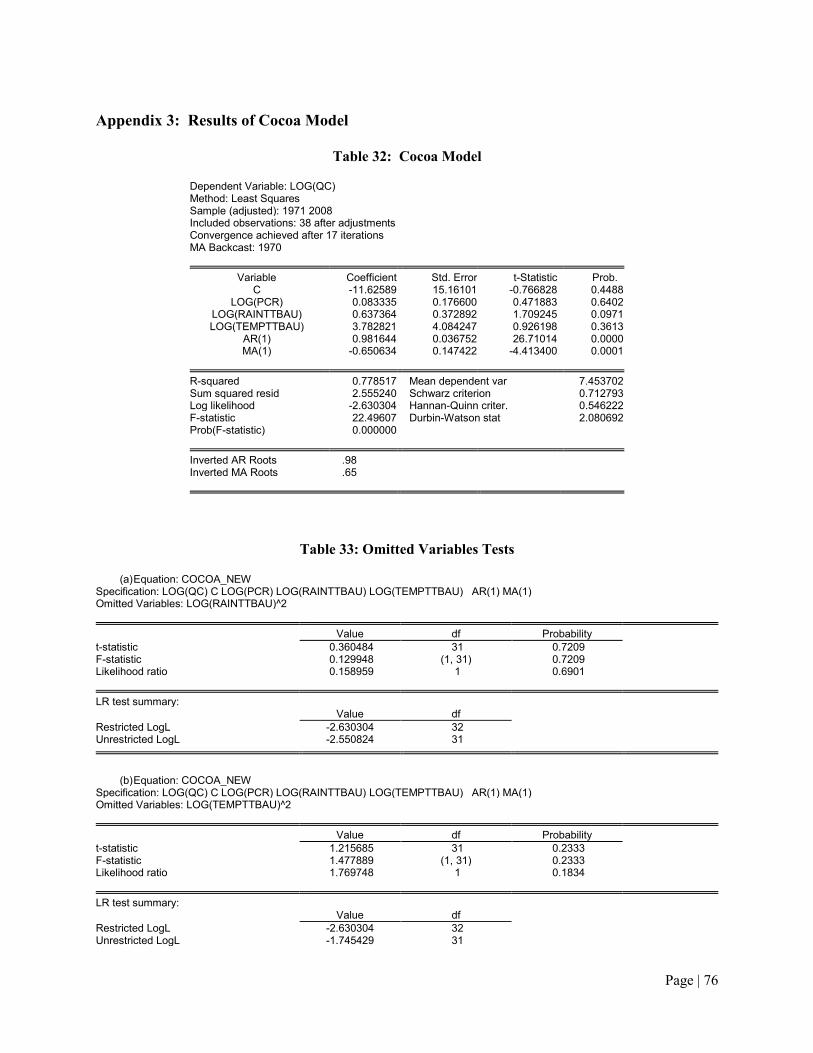
Page | 76

Appendix 3: Results of Cocoa Model

Table 32: Cocoa Model

Dependent Variable: LOG(QC) Method: Least Squares Sample (adjusted): 1971 2008 Included observations: 38 after adjustments Convergence achieved after 17 iterations MA Backcast: 1970

Variable Coefficient Std. Error t-Statistic Prob. C -11.62589 15.16101 -0.766828 0.4488

LOG(PCR) 0.083335 0.176600 0.471883 0.6402 LOG(RAINTTBAU) 0.637364 0.372892 1.709245 0.0971 LOG(TEMPTTBAU) 3.782821 4.084247 0.926198 0.3613

AR(1) 0.981644 0.036752 26.71014 0.0000 MA(1) -0.650634 0.147422 -4.413400 0.0001

R-squared 0.778517 Mean dependent var 7.453702 Sum squared resid 2.555240 Schwarz criterion 0.712793 Log likelihood -2.630304 Hannan-Quinn criter. 0.546222 F-statistic 22.49607 Durbin-Watson stat 2.080692 Prob(F-statistic) 0.000000

Inverted AR Roots .98 Inverted MA Roots .65

Table 33: Omitted Variables Tests

(a) Equation: COCOA_NEW Specification: LOG(QC) C LOG(PCR) LOG(RAINTTBAU) LOG(TEMPTTBAU) AR(1) MA(1) Omitted Variables: LOG(RAINTTBAU)^2

Value df Probability t-statistic 0.360484 31 0.7209 F-statistic 0.129948 (1, 31) 0.7209 Likelihood ratio 0.158959 1 0.6901

LR test summary: Value df

Restricted LogL -2.630304 32 Unrestricted LogL -2.550824 31

(b) Equation: COCOA_NEW Specification: LOG(QC) C LOG(PCR) LOG(RAINTTBAU) LOG(TEMPTTBAU) AR(1) MA(1) Omitted Variables: LOG(TEMPTTBAU)^2

Value df Probability t-statistic 1.215685 31 0.2333 F-statistic 1.477889 (1, 31) 0.2333 Likelihood ratio 1.769748 1 0.1834

LR test summary: Value df

Restricted LogL -2.630304 32 Unrestricted LogL -1.745429 31

Page | 77

Appendix 4: Adaptation Options and Forest Fires

Table 34: Potential Risks and Adaptation Options

(High/Yes=5; Medium=3;Low/No=1) Risk Source Adaptation

Option Evaluation Criteria

Low Cost

Effectiveness

Acceptance to Stakeholders

Endorsement by Experts

Short Time Frame

Institutional Capacity

Size of Beneficiary Group

Ease of Implementation

Adequacy for Current Climate

Potential Positive Social/Environmental Impact

Potential to Sustain Over Time

Score

Water Availability

Rainfall

Use water saving irrigation systems and water management systems e.g. drip irrigation

M H H H H H H H H H H 53

Build on- farm water storage (ponds, tanks etc)

H H H M M H M M H H M 45

Promote water conservation – install on-farm water harvesting off roof tops

H M L M H H H H H H H 47

Install protected agriculture facilities

L H M H M M M L H H M 37

Change agronomic practices e.g. mulching

M H L H H H H M H H M 45

Change water pricing to reflect increasing scarcity

H M L H H M H L H H M 41

Build new dams L H M H L M H L H M M 35 Design and

implement holistic water management plans for all competing uses

M H H H M H H L H H H 47

Repair/maintain existing dams

M H H H H H H H H H M 51

Provide fiscal incentives for

L H M M M L H M H H M 37

Page | 78

Risk Source Adaptation Option

Evaluation Criteria

Low Cost

Effectiveness



Short Time Frame







Score

water conservation

Relocate farms to lands with good agricultural capability

L M M H M M M L M H H 35

Establish germplasm bank of native drought tolerant varieties/ provide quick availability of planting material

L M M H L M H M M H M 35

Mainstream climate change issues into agricultural management

H M H H H H H H H H H 53

Alter crop calendar for short-term crops

H H H H H H H H L H H 51

Promote agricultural diversification

M M H H M M H M H H M 43

Reduce non-native competition by controlling invasive species

L H L H M M H M M H M 37

incidence of drought

Introduce more drought resistant/ tolerate species

L H H H L L H L H H M 37

Adopt improved technologies for soil conservation

H H M H H H H M H H H 51

Implement land policy to retain high quality land

L H H H L H H L H H L 39

Build new desalination plants to meet

L H M M M H H M H H H 43

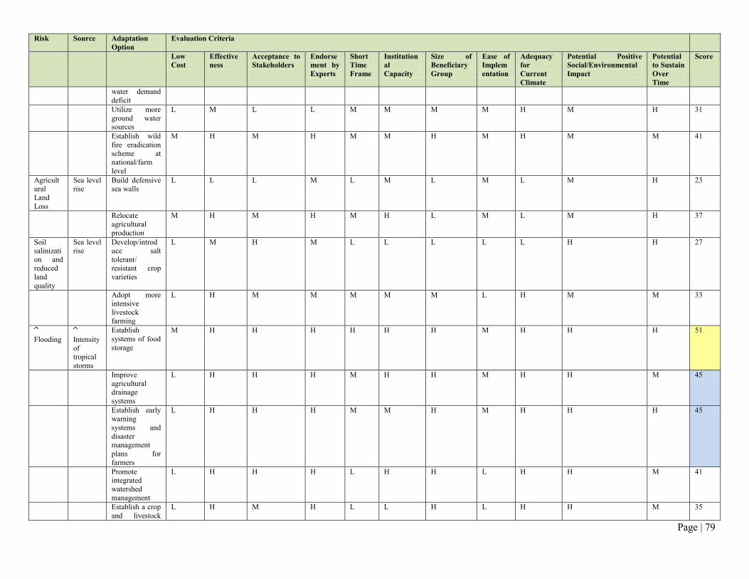
Page | 79


Evaluation Criteria

Low Cost

Effectiveness



Short Time Frame







Score

water demand deficit

Utilize more ground water sources

L M L L M M M M H M H 31

Establish wild fire eradication scheme at national/farm level

M H M H M M H M H M M 41

Agricultural Land Loss

Sea level rise

Build defensive sea walls

L L L M L M L M L M H 23

Relocate agricultural production

M H M H M H L M L M H 37

Soil salinization and reduced land quality

Sea level rise

Develop/introduce salt tolerant/ resistant crop varieties

L M H M L L L L L H H 27

Adopt more intensive livestock farming

L H M M M M M L H M M 33

Flooding

Intensity of tropical storms

Establish systems of food storage

M H H H H H H M H H H 51

Improve agricultural drainage systems

L H H H M H H M H H M 45

Establish early warning systems and disaster management plans for farmers

L H H H M M H M H H H 45

Promote integrated watershed management

L H H H L H H L H H M 41

Establish a crop and livestock

L H M H L L H L H H M 35

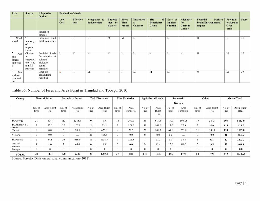
Page | 80


Evaluation Criteria

Low Cost

Effectiveness



Short Time Frame







Score

insurance scheme

Wind speed

Intensity of tropical storms

Introduce wind breaks on farms

H L L M M L H L H H L 31

Pest and disease outbreaks

Change in temperature and rainfall patterns

Establish R&D for adoption of cultural/ biological control measures

L H H H L L H L H H M 37

Sea surface temperature

Establish aquaculture facilities

L H M H H M M M H M M 39

Table 35: Number of Fires and Area Burnt in Trinidad and Tobago, 2010

County Natural Forest Secondary Forest Teak Plantation Pine Plantation Agricultural Lands Savannah/ Other Grand Total

Grasses No. of fires

Area Burnt (Ha)

No. of fires

Area Burnt (Ha.)

No. of fires

Area Burnt (Ha)

No. of fires

Area Burnt(Ha)

No. of fires

Area Burnt (Ha)

No. of fires

Area Burnt (Ha)

No. of fires

Area Burnt (Ha)

No. of fires

Area Burnt (Ha)

St. George 28 1404.7 113 1388.7 0 1.5 14 260.0 46 689.8 87.0 1069.3 15 349.9 303 5163.9 St. Andrew/ St. David

7 23.5 27 107.8 5 73.5 7 174.0 48 164.0 22.0 77.9 2 4.0 118 624.7

Caroni 0 0.0 3 28.5 2 625.0 9 32.5 26 148.7 67.0 233.6 31 100.7 138 1169.0

Victoria 0 0.0 0 0.0 21 455.6 0 0.0 0 0.0 0.0 0.0 0 0.0 21 455.6

St. Patrick 2 44.8 20 639.0 11 1551.7 7 122.5 1 27.2 5.0 54.4 1 33.7 47 2473.3 Nariva/ Mayaro

1 1.0 7 64.4 0 0.0 0 0.0 24 45.4 15.0 340.3 5 9.8 52 460.9

Tobago 0 0 0 0 0 0 0 0 0 0 0 0 0 0 0 0.0

TOTAL 38 1474 170 2229 39 2707.3 37 589 145 1075 196 1776 54 498 679 10347.4

Source: Forestry Division, personal communication (2011)

Documents

THE IMPACTS OF CLIMATE CHANGE ON AGRICULTURAL …