Embed Size (px)
Citation preview

DSpace Institution
DSpace Repository http://dspace.org
Structural Engineering Thesis
2020-04
THE IMPACT OF SEDIMENT ON
RESERVOIR VOLUME CHANGE, (THE
CASE OF KOGA RESERVOIR, UPPER
BLUE NILE BASIN, ETHIOPIA)
HANIBAL, GENET
http://ir.bdu.edu.et/handle/123456789/12473
Downloaded from DSpace Repository, DSpace Institution's institutional repository

BAHIR DAR UNIVERSITY
BAHIR DAR INSTITUTE OF TECHNOLOGY,
SCHCOOL OF RESEARCH AND GRADUATE STUDIES
FACULTY OF CIVIL AND WATER RESOURCES ENGINEERING
M.SC. THESIS: THE IMPACT OF SEDIMENT ON RESERVOIR
VOLUME CHANGE,
(THE CASE OF KOGA RESERVOIR, UPPER BLUE NILE BASIN,
ETHIOPIA)
BY: HANIBAL GENET
APRIL, 2020
BAHIR DAR, ETHIOPIA

BAHIR DAR UNIVERSITY
BAHIR DAR INSTITUTE OF TECHNOLOGY,
FACULTY OF CIVIL AND WATER RESOURCES
ENGINEERING
THE IMPACT OF SEDIMENT ON RESERVOIR VOLUME
CHANGE
(THE CASE OF KOGA RESERVOIR, UPPER BLUE NILE BASIN,
ETHIOPIA).
BY: HANIBAL GENET
A thesis submitted in partial fulfillment of the requirements for the
Degree of Master of Science in Hydraulic Engineering
Advisor: Bitew Genet (Ass. Prof.)
April, 2020
Bahir Dar, Ethiopia
@2020 Hanibal Genet

i

ii

iii

iv
Abstract
Ethiopia has long since been an area strongly affected by sedimentation. Sediment
accumulation modeling in the constructed dam is an obstacle by the lack of historic
sediment concentration data in developing countries. Nevertheless, the purpose of dams is
affected by sedimentation. Water balance models then used to simulate sediment
distribution in the reservoir. This often results in the estimation of sediment variability that
is not identically distributed throughout the time. To show the temporal distribution of
sediment in the Koga reservoir water balance model was used. It is likely that the volume
of the Koga reservoir would reduce over time due to reservoir sedimentation. This reservoir
sedimentation could mean a decrease in water supply for the irrigation project in the future.
In addition, the method applies existing and future knowledge of sedimentation and annual
climate variability relative to the Koga reservoir. Data collection of hydrology,
meteorology, and irrigation water supply for the project site have been statistically
compared and arranged as an input data source to fit the model. The volume change was
incorporated into the water balance model. According to the water balance model result a
reservoir volume reduction of 0, 5, 10, and 15Mm3 leads to minimum water storage of 6.7,
4.8, 2.9, and 0 Mm3 respectively in May. Because the minimum result appears just the end
of the winter season as this is the time of year when the reservoir has been in the largest
use. The thesis result shows sediment accumulation increase reservoir storage volume
decrease. From this study, it is possible to be concluded that the dam is capable of providing
enough irrigation water around 2027 E.C.
Keywords: dam, Sediment rate, Koga Reservoir, Useful period, water balance model

v
Acknowledgment
Much appreciation is expressed for my advisors Mr. Bitew Genet. (Ass. Prof.), his smart
and sweet advice put me on the journey of education and assisted me to begin this final
thesis. Again, I would like to express my thanks to the Ministry of Water, Irrigation, and
Energy for the data assistance given me in data collection. Acknowledgment is expressed
to the staff of Amhara Water Works Design and Supervision Enterprise and Amhara Water
resource and Energy bureau. Special thanks are due to my colleagues, family, relatives,
and friends for their cooperation to accomplish this study. Finally, I am also thankful to all
those who are not mentioned here but have helped and supported me in order to achieve
this research work successfully.

vi
List of Abbreviations
BNB Blue Nile Basin
GDP Gross Domestic Product
GIWR Gross Irrigation Water requirement
FAO Food and Agriculture Organization
ICTZ Inter-Tropical Convergence Zone
IPCC Intergovernmental Panel on Climate Change
Kc Crop coefficient
Kms Kilometers
m Meter
masl Mean Above Sea Level
mm Millimeter
Mm3 Million meter cube
M3/s Meter Cube per Second
MoWIE Ministry of Water, Irrigation, and Electricity
NMSA National Meteorological Services Agency
SN Scenarios
SRES Special Report on Emission Scenario
WEAP Water Evaluation and Planning System
WWDSE Water Works Design and Supervision Enterprise
NSR Night Storage Reservoir

vii
Table of Contents
Declaration ......................................................................... Error! Bookmark not defined.
Abstract .............................................................................................................................. iv
Acknowledgment .................................................................................................................v
List of Abbreviations ......................................................................................................... vi
List of Figure.......................................................................................................................x
List of Tables ................................................................................................................... xiii
1. Introd1uction ....................................................................................................................1
1.1. Back ground ..............................................................................................................1
1.3 Statement of the problem ...........................................................................................2
1.4 Scope of the Study......................................................................................................3
1.5 Significant of the Study ..............................................................................................3
1.6 Research questions .....................................................................................................4
1.7 Objectives of the Study ..............................................................................................4
1.7.1 General objective .................................................................................................4
1.7.2 Specific objectives ...............................................................................................4
1.8 Thesis outline .............................................................................................................4
2 Literature review ...............................................................................................................4
2.1 Sedimentation on Koga reservoir volume change......................................................4
2.2 Reservoir lifetime .......................................................................................................5
2.3 Crop Water demand ...................................................................................................5
2.4 Climate Change Impacts on Reservoir .......................................................................7
2.5 Decreasing Sediment Inflow into the Reservoir ........................................................7
2.6 Suggested and real cropping system ..........................................................................8
2.7 Users Bias on cropping system ....................................................................................10

viii
2.8 The Dam and reservoirs ...........................................................................................10
2.9 The project area and the canal ..................................................................................11
3 Materials and Methods ....................................................................................................13
3.1. Description of the Study Area .................................................................................13
3.2 Location ....................................................................................................................13
3.3 The hydrology and geology of Upper Blue Nile Basin ............................................14
3.4 The geology of the UBNB can be divided into three different part:- ......................14
3.5 Climate and rainfall data ..........................................................................................15
3.6 The water balance Model and its components .........................................................16
3.6.1 River discharge Inflow (Qin) .............................................................................18
3.6.2 Rainfall (P) ........................................................................................................19
3.6.3 Evaporation (E) of the Bahir Dar, Merawi, and Koga site ................................20
3.7 Outflow (Qout) ...........................................................................................................23
3.7.1 Release discharge for Maintenance and sediment flushing ...............................23
3.7.2 Environmental compensation flow ....................................................................23
3.7.3 Irrigation water release flow .................................................................................26
3.7.3.1 Crop water demand (CWR) analysis ..............................................................26
3.7.4. Secondary data collection.....................................................................................28
3.7.5 Data analysis techniques .......................................................................................28
3.8 Model scenarios........................................................................................................28
3.8.1 Model Scenario 1 ...............................................................................................29
3.8.2 Model Scenario 2 ...............................................................................................29
3.8.3 Model Scenario 3 ...............................................................................................29
3.8.4 Model Scenario 4 ...............................................................................................29
4 Model scenarios Results and discussion .........................................................................30
4.1 Model scenarios Results ...........................................................................................30

ix
4.1.1 Scenario 1 Reservoir volume under normal states ............................................30
4.1.2 Scenario 2 reservoir volume change by 5Mm3 ..................................................30
4.1.3 Scenario 3 reservoir volume change by 10 Mm3 ...............................................31
4.1.4 Scenario 4 reservoir volume change by 15 Mm3 ...............................................32
4.2 Model scenario Discussion ......................................................................................33
4.2.1 Model scenario 1 Reservoir volume under normal states ..................................33
4.2.2 Model Scenario 2 reservoir volume change by 5Mm3 ......................................34
4.2.3 Model Scenario 3 reservoir volume change by 10Mm3 ....................................35
4.2.4 Scenario 4 reservoir volume change by 15Mm3 ................................................36
4.2.5 Model scenario summary ...................................................................................37
5. Conclusion and recommendation ...................................................................................39
5.1 Conclusion ................................................................................................................39
5.2 Recommendations ....................................................................................................40
6. Reference .......................................................................................................................41
7. Appendix ........................................................................................................................60
Appendix A ....................................................................................................................60

x
List of Figure
Figure 1 Area coverage of dry season cropping system ......................................................9
Figure 2 the percentage and project area for each crop .......................................................9
Figure 3 the current dry season percentage of the project area for each crop. ..................10
Figure 4 the Koga reservoir and irrigation location. ..........................................................13
Figure 5 Merawi meteorological stations Tmax and Tmin. ...............................................15
Figure 6 Merawi meteorological stations rainfall and eto. ................................................16
Figure 7 Reservoir inflows and outflows; parameters for the water balance model .........17
Figure 8 Monthly Qin values used in the water balance model. ........................................19
Figure 9 Monthly Precipitation values used in the water balance model. .........................20
Figure 10 Monthly evaporation values used in the water balance model ..........................21
Figure 11 Comparison of monthly Eto, Ecal, and Koga E of the site. ...............................23
Figure 12 Water released from the reservoir for environmental compensation flow for each
month given in Mm3 (Ministry of Water Resources, 2006). .............................................25
Figure 13 Water released reservoir for partial environmental compensation release flow for
each month given in Mm3 (Ministry of Water Resources, 2006). ....................................25
Figure 14 Comparison of crop irrigation water demand CIWR from the design report
scenarios .............................................................................................................................27
Figure 15 Reservoir volume under normal states ..............................................................30
Figure 16 gives reservoir volume reduction by 5Mm3 for each month as computed in the
water balance model. .........................................................................................................31
Figure 17 gives reservoir volume reduction by 10Mm3 for each month as computed in the
water balance model. .........................................................................................................31
Figure 18 gives reservoir volume reduction by 15Mm3 for each month as computed in the
water balance model. .........................................................................................................32
Figure 19 Reservoir volume under normal state ................................................................34

xi
Figure 20 Reservoir volume by 5Mm3 reduction ..............................................................35
Figure 21 volume reductions Reservoir by 10 Mm3. ........................................................36
Figure 22 Reservoir volume by 15Mm3 reduction ............................................................37
Figure 23 summary of volume change due sediment accumulation in different year from
scenario 1-4 ........................................................................................................................38

xii
List of Tables
Table A1 suggested cropping plan for the wet and dry season (Ministry of Water
Resources, 2006) ................................................................................................................60
Table A2 Actual cropping pattern for dry season (Ministry of Water Resources, 2006). .60
Table A3 dry season proposed cropping system (%).........................................................60
Table A4. Reservoir simulation runs. PIA is the potential irrigated area in hectares
(Ministry of Water Resources, 2006) .................................................................................61
Table A5. Command Areas and their Sizes (Ministry of Water Resources, 2006). The
addition of the Tekel Dib extension area is designed for the future. .................................61
Table A6 Comparison of monthly evaporation between Bahir Dar meteorological station,
calculated and the Koga site. .............................................................................................62
Table A7 Data for Koga river inflow given by design reports Nile (Mott MacDonald, 2004)
............................................................................................................................................62
Table A8. Precipitation data for Bahir Dar (Ministry of Water Resources, 2004). ...........62
Table A9 Crop Water Usage Values estimated by Mott MacDonald in the project
report ..................................................................................................................................63
Table A10 these different scenarios modify the variables in the water balance equation to
represent changes in sedimentation. ..................................................................................63
Table A11 these different scenarios modify the variables in the water balance equation to
represent the partial environmental release. .......................................................................64
Table A12. Monthly compensation flows (Ministry of Water Resources, 2006). .............64
Table A13 Data for Crop Water Usage Calculations (Ministry of Water Resources,
2006) ..................................................................................................................................65
Table A14 Scenarios I-IV net irrigable are and. GIWR of the whole irrigated area (Ministry
of Water Resources, 2008). ................................................................................................67

xiii
Table A15 Growing season lengths in months and total irrigation water requirements in
mm for selected crops as estimated by ..............................................................................69
Table 16 Area covered by each crop ..................................................................................69
Table 17 Average monthly crop water requirement of cultivated crops in the project .....70

xiv

1
1. Introd1uction
1.1. Back ground
Ethiopia has long since been an area strongly affected by drought. Although there is a
relatively large amount of fresh water present in the country, (110 billion m3 of water are
discharged out of the country each year) variability in rainfall and lack of infrastructure
lead to the result that most of the population is undersupplied with water (Marx, 2011).
The upper Blue Nile Basin, known as the Abay River Basin in Ethiopia, has an estimated
irrigation potential of 760,000 ha yet actual irrigated land use was measured to be a mere
30,000 ha (Moges, 2010). Dam building balances the increased flow depth and decreased
flow velocity of a reservoir reduces the sediment transport capacity and causes
sedimentation. Silts carried into a reservoir may deposit throughout its full volume, thus
rapidly raising the bed elevation and causing addition. The layer of deposition generally
starts with a deltaic formation, mainly contains coarser sediments in the reservoir bed level.
The flow currents may transport finer sediment particles down to the reservoir. Reservoir
sediment accumulation was a complex process that varies with catchment sediment yield,
rate of motion, and form of accumulation. Reservoir silt accumulation depends on the river
morphology, flood occurrence, reservoir dimension and operation, flocculation potential
silt deposition, flow density currents, and possible watershed changes over the life
expectancy of the reservoir (Raghunath, 2006).
Agriculture employs 85% of the workforce in Ethiopia (CIA World Fact Book, 2012)
and is the largest economic activity (as of 2004) at 46.3%, with services being the second
most prominent at 41.2% of a Gross Domestic Product (GDP) per capita of 1000 USD (UN
Ethiopia, 2012). Despite this fact, the productivity of agriculture in Ethiopia is only 1.2
tons per ha, one of the lowest in the world making food security a serious problem for a
country with a fast growing population(Marx, 2011).
Development of irrigation projects is listed as a prime tool to ensure food security at the
household level. The Ministry of Water Resources sees expansion of irrigated agriculture
as a way to provide food security for a fast growing population. The Koga Dam is a key
project for the Ethiopian government, as a step towards achieving food self-sufficiency at

2
both national and regional levels for a country that has a history of draughts and famine
(Ministry of Water Resources, 2004). Population growth in Ethiopia is projected to be 2.5%
per year, while growth of crop yields is only increasing 1.4% per year (1960-2001),
creating a declining food availability per capital from domestic production(Ministry of
Water Resources, 2008).
On the household step, farmers in the Koga region stand to gain a lot of advantage from
this large irrigation system. The average landholding is 1.68 ha with this size of command
area, a family using a rain-fed irrigation system can have a net income of around 6000
Ethiopian birrs. But in the irrigated system, net income increases to 20000-26000 birr,
about four times as much as under the rain-fed system(Marx, 2011). Sedimentation is a
problem for many reservoirs around the world, and especially in this region. The volume
of the Koga reservoir will likely decrease over time due to reservoir sedimentation. An
enhanced variability in sediment is also predicted for the region which could mean years
with below-average rain. Damming of rivers causes major changes concerning water
availability in the watershed, for example, evaporation increases while runoff decreases.
All crops in the Koga site require water for irrigation during the Dry Season (vorosmarty,
1997).
For this site, it is important to know the irrigation water volume of the reservoir in order to
plan what crops to grow and how much land can be irrigated, which depends on the amount
of irrigation water available in the reservoir. This thesis aims to see the way the change in
maximum reservoir volume, in addition to a change in temperature, precipitation, and
evaporation, affected the irrigation water volume of the reservoir. When reservoir volume
reaches zero and is unable to supply any water is of special interest. An annual water
balance assessment of the Koga dam throughout the entire course of a hydrologic year was
done in order to estimate current and future annual changes in the reservoir’s volume.
Water is not only influenced by human activities, but also by natural factors, such as
temperature, precipitation, and evaporation change (IPCC, 2007).
1.3 Statement of the problem
Reservoir sedimentation is a harmful off-site cause of climate change with large
environmental and economic factors. The threat of sedimentation problems and

3
management methods vary widely from time to time. In the case of the Koga reservoir,
there is an inflow of a huge amount of sediment to the reservoir because of agricultural use,
domestic water supply, deforestation, overgrazing, and geological formation. The research
to study reservoir siltation and sediment change of a dam is a huge challenge for a hydraulic
engineer to determine the useful life of a designed structure and to predict the amount of
sediment settle in the reservoir.
1.4 Scope of the Study
This research was carried out at The Koga reservoir which was built on the Koga River,
about 35km south of the city of Bahir Dar and Lake Tana, outside the village of Merawi,
in the West Gojam zone of the Amhara region. The focus of this study was mainly on
computing the decrease of the reservoir volume due to sediment increase and to compare
the supply irrigation water volume of the reservoir with the crop water requiremen in
order to know a critical/minimum / reservoir supply volume for a given month.
1.5 Significant of the Study
Knowing about the effect of sediment change helps to take a lot of measures that protect
sediment yield entering into the Koga reservoir. The thesis was created announcement for
the farmer and the government to know about the role of sediment change on sediment
yield in the reservoir. In addition to that, the research will give warnings to the farmer and
the government to do different watershed protection activities to control the role of
sediment yield in the reservoir for the future. However, sediment variation would further
obliterate the periodic and chronic shortfall of water and result in repeat droughts in some
places in some time maybe a month. Research on sedimentation problems is important for
the user to know the current and future crop cover and supply irrigation water resources.
Promisingly my work would be an input for the responsible persons in the management,
crop pattern, and further building of the suggested new dam. It also had its own significance
towards the local farmer economy by the proper management of the watershed. This work
was intended for the user by Engineers, Scientists, and water Resource Managers to support
in formulating sediment management plans for reservoirs, in order to satisfy the objective
of plan a reservoir sustainable.

4
1.6 Research questions
What are the effects of sediment change on the reservoir volume?
How to estimate reservoir volume by using the the water balance model?
1.7 Objectives of the Study
1.7.1 General objective
The general objective of this study is to investigate and analyse the impact of sediment
accumulation on koga reservoir.
1.7.2 Specific objectives
To determine the temporal distribution of sediment deposition in the reservoir.
To identify the critical water shortage month in the reservoir.
To evaluate impact of sediment change on reservoir
To evaluate capacity of reservoir to support the command area
1.8 Thesis outline
The final thesis composed of eight main titles and each title has a section and sub-section
to describe the contents i.e.:-
Section1: Introduction
Section 2: Literature review: - Insight learning all research review.
Section 3: Methods/methodology (description of the study area, method, and materials).
Section 4: Result and Discussion: - Result obtained by water balance model including
predicting the use full life of the reservoir, sediment yield estimation from the reservoir,
current and future sediment deposited volume and their discussion.
Section 5: Conclusions and recommendations.
Section 6: References and Section 7 appendixes.
2 Literature review
2.1 Sedimentation on Koga reservoir volume change
Sediment travels in the stream as suspended load (fine particles) in the flowing water, and
as bed load (large particles), which moves along the channel bottom. Sometimes, the

5
particles (small particles of sand and gravel) roll by bouncing along the bed, which is
known as ‘saltation’, which is a critical stage between the bed and suspended load. The
particle, which travels as bed load at one section may be in suspension at another section.
At the time sediment-laden water reaches a reservoir, the velocity and turbulence are
greatly minimized. The dense fluid-solid composition along the bottom of the reservoir
travels slowly in the form of a density current or stratified flows, i.e., a diffused colloidal
suspension having a density that slightly varies from that of the main body of reservoir
water, due to dissolved minerals and temperature, and hence does not diffuse readily with
the reservoir water (IPCC, 2007).
Smaller particles may be settled near the base of the reservoir. Some of the density currents
and settled sediments near the base of the reservoir can be flushed out by operating the
sluice gates. The modern multipurpose reservoirs are operated at different water stages,
which is high in the deposition and movement of silt in the reservoir (Raghunath, 2006).
2.2 Reservoir lifetime
The capacity of the reservoir can also be minimized by sediment accumulation. This
happens because the flow velocity reduces when the water passes through the reservoir.
The consequence is reservoir volume minimization, and the maximization of life
expectancy of a reservoir is therefore limited. The design of a dam is based on future time,
important demographic and hydrological parameters, but with the present evidence of
climate change, such design could be a shortage if supply and demand condition varies.
One way of exercising if the reservoir is inadequate is to enlarge the reservoirs, if it is
topographically and hydrologically feasible(Britannica, 2010).
2.3 Crop Water demand
The quantity of irrigation water taken from the reservoir each month depends upon the
irrigation water requirements of the crops grown in the irrigable areas, as well as the
irrigation methods used. The way used to irrigate the fields in the Koga project area and
has a predicted efficiency of 50% (USGS, 2000). This means the water supplied for
irrigation will be smooth twice the evapotranspiration of any given crop. The gross
irrigation water demand (GIWR), the total amount of water required for irrigating, is
affected not only by the amount of precipitation available to the crops but also depends

6
upon what type of crop is irrigated how much area is under irrigation, and in what relation
crops are irrigated. All crops had different water demands due to different natural amounts
of evapotranspiration. Crops irrigated in the irrigable areas include wheat, maize, potato,
green pepper, onion, barley, beans, haricot beans, abish, fasolia, cabbage, tomato, carrot,
beatroot, teff, shallots, millet, noug, and garlic. Furrow irrigation is one of the oldest ways
to irrigate, probably the first system used by humans, and is still largely in use today
(USGS, 2000).
It includes transport of water to the field through farmer dug ditches in the case of the Koga
reservoir irrigable area (field observation). The water then travels the field between the
rows of crops and is absorbed by the crops after infiltrating the soil. Furrow irrigation is
less effective than other systems of irrigation such as drip irrigation. It is predicted that
only 50% of the water used in-furrow irrigation feeds the crop. Much amount is loosened
by the runoff, evaporation, and infiltration of uncultivated areas (USGS, 2000). In the Koga
irrigation project area, furrow irrigation is the system used due to the fact that it is relatively
easy and cheap. The efficiency of water use in irrigation is governed by three root zone
processes; macropore formation, fertilizer application systems, and depth of root uptake.
Knowledge of macropores from root decay and wormholes enhances the flow rate through
the soil and channelize the flow, and make the infiltration less uniform as the flow is
channelized. Macro pores called planar voids have also happened from soil expansion and
contraction cycles that affect water motion. The depth at which roots needed the most water
can be quickly controlled by plants in response to irrigation. When the irrigation water is
applied, near the surface roots become most active created that the volume of water
extracted by roots is much near the surface and shows a decreasing trend with depth.
Fertilizer use in the Koga command area is reduced (Clothier, 1993).
In the study on the efficient use of irrigation water done by (Clothier, 1993). It was
concluded that the most efficient system of irrigating plants that depend on the three root
zone processes stated above was to use little amounts of water and irrigate repeatedly. If
flood irrigation is used such as in the Koga watershed, then the soil should be controlled in
a way that micropores are eliminated or decreased before irrigation. Drainage loss from
micro pores controls two problems; both the loss of water from the root zone that could

7
have been used to grown crops and the enhanced pollution of ground- and surface water
sources (Clothier, 1993).
2.4 Climate Change Impacts on Reservoir
Water is communicated in all parameters of the climate system. Findings of the (IPCC,
2001) high suggests that water resource answered to the global warming in ways that
negatively impacted the water availability and water supplies. The decrease in the runoff
volume will lead to the reduction in the inflow to the reservoirs accordingly; a longer period
might be needed to fill the reservoir. As the result of the enhance in temperature, the rate
of evaporation from the reservoir open water surface may maximum and this may occur
the reservoir to fail to supply at least enough amount of water required because of its
shortage in the active storage water stage (Habtom, 2009).
The most acciaccatura climate drivers for water accessibility are rainfall, temperature, and
Evaporative (justified by net radiation at the ground, atmospheric humidity and wind speed,
and temperature). Water evaporated from the surface and transpired from plants called
evapotranspiration rises with air temperature. These make a huge decrease in runoff and
increase water shortages as a result of a combination of increased evaporation and reduced
precipitation. The repeated and severity of droughts could increase in some areas as a result
of a decrease in precipitation, more frequent dry spells, and higher ET (Kenneth, 1997).
2.5 Decreasing Sediment Inflow into the Reservoir
Sediment accumulation in reservoirs cannot be actually controlled but it can be reduced by
exercising some of the following measures:
I. Reservoir area, which are productive sources of sediment should be avoided.
II. Adopting soil-conservation mechanism in the watershed, as the silt originates in the
catchment area.
III. Agronomic soil conservation methods like cover cropping, strip cropping, contour
farming, suitable crop rotations, application of green manure (mulching), proper control
overgraze lands, terracing, and benching on steep hill slopes, etc. retard overland flow,
increase infiltration and decrease erosion.
IV. Contour trenching and afforestation on hill slopes, contour bundling gully plugging by
check dams, and stream bank control by the use of spurs, revetments, vegetation cover, etc.
are the main engineering measures of soil conservation mechanism.
V. vegetation cover on the land decreases the impact force of raindrops and reduce erosion.

8
VI. Sluice gates constructed in the dam at the various stage and reservoir operation, allow
the discharge of fine sediments without giving them time to reach the bottom.
VII. Sediment accumulation in tanks and small reservoirs may be avoided by excavation,
dredging, draining, and flushing either by mechanical or hydraulic methods and sometimes
may have some sales value.
2.6 Suggested and real cropping system
There is two crop period in a year, one classifying under the rain-fed summer season, and
the other classifying under the winter season that is only made possible by using irrigation.
The weather in the Koga command area is controlled by the motion of the ITCZ and like
most tropical regions it adopts a summer season (June-September) and dry season other
than the wet period. The precipitation during the summer season is assumed to be sufficient
to supply all of the crop water requirement, so no additional irrigation from the dam is
planned during the peak of the rain season. The consultants for the Koga irrigation project,
Mott MacDonald, provide that the crops irrigated during the summer season should have
short growing times in order to reduce the amount of irrigation water required at the end
of the wet season when the rainfall reduces below levels that can support rain-fed irrigation
(Ministry of Water Resources, 2004).
The suggested proportion of crops for each growing season in order to maximize profits
and reduce irrigation water requirements differs smoothly from the real cropping pattern
in place due to variation in crop prices and farmers' personal decisions. The suggested
cropping plan for the summer season and real cropping for the dry season is given in Figure
1-3 below. Values are also listed in Appendix A Tables A1, A2, and Table A3 wet and dry
season suggested cropping system and dry real cropping system respectively (Ministry of
Water Resources, 2006).
The proposed cropping pattern for the wet season is comprised of maize, millet, noug, and
teff. Most of the command area during the current dry season was irrigated with potato,
wheat, barley, maize, onion, and garlic. Crop distribution is different over the whole
command area as farmers ultimately choose what they wish to irrigate. There may also be
smooth differences between irrigable areas in soil quality influencing which crop is most
productive. Each irrigable area, therefore, has a different crop composition distribution to
the total ratios of crops throughout the whole command area. The actual amount of area

9
sown was less than the designed amount of the full 7000 hectares as this is the first year
that the project is fully operational and irrigation method efficiency, as well as farmer
competence, were still not perfect (IPCC, 2001).
Figure 2 the percentage and project area for each crop
20%
20%
20%
40%
wet season suggested cropping system(%)
maize
millet
noug
teff
Figure 1 Area coverage of dry season cropping system
16%
47%12%
7%
18%
dry season suggested cropping system(%)
potato
maize
shallote
peppers

10
Figure 3 the current dry season percentage of the project area for each crop.
2.7 Users Bias on cropping system
The Koga irrigation project office in Malawi does a planed what crops to grow each season
based upon market prices and water usage and supplied a list of possible crops to be
irrigated to the users. The users then make the final adjustment of what they will grow by
deciding from this list. A combination of reference from the project office and farmer
education concerning water efficiency would hopefully put a huge emphasis on efficient
water use when adjusting what crops to irrigate in the future. Users choose what crops to
irrigate each season based on many factors, practices with the crop, seed availability, labor
availability, environmental factors such as soil conditions and climate, government
policies, and availability for their consumption. Nevertheless, the huge factor influencing
their decision is relative productivity. For the Koga irrigation project users, the most
sufficient crop in terms of net returns per area is wheat (Ministry of Water Resources,
2008).
2.8 The Dam and reservoirs
The Koga dam is constructed on the Koga River, a tributary of the Upper Blue Nile
releasing into Lake Tana in Northern Ethiopia. The Koga river is the only river that
releasing water into the reservoir, which upon completion, had a volume of 83.1 Mm3 and
a surface area of 1750 ha ( Marx, 2011).
31.37
19.556
3.2310.1740.108
0.011
0.005
41.559
0.55
0.2290.001
0.004
1.215 1.378 0.601
dry season real cropping system(%)
wheat
Barely
Maize
bean
haricot bean
abish
fasolia

11
There are two outlets in the reservoir to give three purposes:- The first is the bottom outlet,
which uses as an emergency and environmental outlet. The maximum discharge from this
outlet is 31m3/s which is used to release the flow during emergencies or for maintenance.
Water may be flow for maintenance purposes in order to do maintenance on the dam
structure or to release out settled sediment. Sediment releasing happens once a year and
operates at maximum discharge for 30 minutes, releasing 55,800 m3 of water. When
maintenance does not happen, this outlet is used for environmental monthly balanced
flows. These flows change depending upon the month in the amount of water discharged.
Nevertheless, the outlet is set at a max discharge rate of 1m/s The reservoir covers a total
command area of 7000 ha (Ministry of Water Resources, 2008).
The second outlet in the dam uses the irrigation canal (Andualem, 2012). According to a
report from United Nations Environment Programm (UNEP, 2000) called “Climate
variability and Dams”, dams have two roles regarding climate change. They can be a source
of greenhouse gases; both carbon dioxide and, if the water at the bottom of the reservoir
becomes anaerobic, they could also emit methane gas. Another aspect of dams is that they
can be used as flood control infrastructures and if precipitation intensity increases due to
climate variability such infrastructure can save lives. A similar report tells that dams
themselves are affected by climate variability. High temperatures create high evaporation
and increased precipitation intensity would enhance the sediment transport to dams. Both
of these impacts decrease the capacity of the dam(UNEP, 2000).
2.9 The project area and the canal
The main canal receives water from the reservoir at a maximum rate of 9.11m3/s. Which
supply a series of 10 secondary canals it then provides water to multiple tertiary canals.
User dug quaternary canals transport water from the tertiary canals to the fields (site
observation). The Koga irrigation command area can be broken into four different units.
Arranging from largest to smallest, these are:- Command areas, Blocks, units, and Fields.
Command/irrigable/ areas are irrigated by a secondary canal dividing on of the main canal.
Then it is made up of blocks and can be anyplace from 220 ha to more than 1000 ha. Blocks
are areas feed by tertiary canals that receive water from the secondary canals. Blocks are
made up of multiple units and their size is different, from>100 ha to between 20 and 65 ha

12
in size. Units are groups of fields and can be the product of 2 or 4. Nevertheless, ideally
made up of 8 fields and ranges from 8 to 16 ha in size. Fields are the smallest unit in the
command area, usually, 2 ha in size, and Fields are irrigated using furrow
irrigation(Ministry of Water Resources, 2008).
All of the fields within a unit would be irrigated on a periodic cycle during which each
field is irrigated once every 8 days. If a unit is smaller than 8 fields, irrigation water coming
into the unit would be blocked off after all fields have been irrigated and the additional
water has used another place in the block until it is time for the periodic to begin again. At
max crop supply, fields operate on a schedule of 12 hours of irrigation from the irrigation
stream (Ministry of Water Resources, 2004).
Night Storage Reservoirs (NSR) are another design feature found in the command area and
control how much water is usable in the secondary canals, effectively doubling the amount
of water used from the main canal (Ministry of Water Resources, 2004). The discharge
from the NSR provides 50% of the maximum required to discharge for the fields. The
additional 50% comes directly from the main canal (Lema, 2012).
Table A3 in Appendix A lists the different command areas and their sizes. In addition to
these two outlets, there is a spillway in the place, if the dam volume should reach more
than its full volume of 83.1 million cubic meters (Mm3), excess water would be flushing,
thus keeping the reservoir volume from filling overcapacity. The Ministry of Water
Resources in Ethiopia has predicted in its Cost Recovery Study for the Koga Irrigation
Project that the irrigation demand of this area of 7000 ha can be fully met if the volume of
the reservoir is in 80 Mm3 and the rest is dead storage for aquatic life i.e 3.1 Mm3. Table
4 in Appendix A, gives values for 10 different model runs done by the Koga engineers
showing the potential irrigation area in ha for the reservoir with 80% reliability. Averaging
all these runs gives a value of 6665.4 ha for the amount of area that could potentially be
irrigated. This is less than the original value of 7000 ha. If these estimations are correct
then the reservoir could be at risk if the volume were to decrease The design volume of the
reservoir is over this recommended value (Ministry of Water Resources, 2006).

13
3 Materials and Methods
3.1. Description of the Study Area
3.2 Location
The Koga catchment lies within the UBNB, in the headwaters of the Upper Blue Nile
Basin. Monthly flow throughout the year varies with the precipitation system and thus the
minimum flow turnaround is during April and the maximum flow turnaround is during
August. The Koga reservoir was built on the Koga River in the Koga watershed, about
35km south of the city of Bahir Dar and Lake Tana, outside the village of Merawi, in the
West Gojam zone of the Amhara region. The dam was built as part of a project to enhance
food security in the country which is poorly low at the moment due to change in sediment,
rainfall, and dependence upon rain-fed agriculture by nearly 90% of the 600,000 people
living in the catchment. It was the first large scale project to be built in the UBNB since
1987 and the first in a series of planned projects (Eguavoen, 2011) and an effective pilot
project as the effectiveness of the Koga project may influence future projects still at the
planning level The wet(rainy) season (July-September) generates about 70% of the runoff
contributing the Koga River (Mott MacDonald, 2004).
Figure 4 the Koga reservoir and irrigation location.
Command
area Koga reservoir

14
3.3 The hydrology and geology of Upper Blue Nile Basin
The precipitation in the UBNB was guided by the Inter-Tropical Convergence Zone’s
migration over the region, which receives moisture from the Indian and Atlantic oceans.
Rainfall ranges between 800 and 2200 mm annually. Most of this Rainfall falls during the
wet season, which takes place from (June – September). The dry season lasts from
(December – May) which receives the smallest amounts of precipitation. This water
collected in the watershed produces an outlet flow of 49.4 G m3 yr-1 at the Sudanese border
(Gebrehiwot, 2010). At the time it reaches the Aswan Dam in Egypt, the Blue Nile accounts
for 62 percent of the flow at that point (Ministry of Water Resources., 1998)
3.4 The geology of the UBNB can be divided into three different part:-
√ Exposed crystalline basement rock covers 32% of the basin,
√ Sedimentary formations compose 11% and volcanic,
√ Formations make up the remaining 52 percent of the catchment.
The major soil type is clay vertisol, which covers around 15% of the region (Gebrehiwot,
2010). Vertisol can be defined as the main type of shrinking and expanding clay. This
movement in the clay can cause cracks to form when it dries and is very susceptible to
erosion (Gebrehiwot, 2010) The geology in the project site are mainly alisols type soils,
with light to medium composition. They are leaky, with a relatively high infiltration rate.
The soils had a fixed irrigation size of (2-4l/s) (Ministry of Water Resources, 2008).
The majority of the soils are very fine (silt-clay) category. Usable water in the root region
was found to be 187mm per meter of soil and the adopted management allowed depletion
level is 30-60% of the important moisture in the effective root zone, depending on the type
of irrigated land. 87% of the irrigation area has been categorized as silty clay soils best for
irrigation. Infiltration is available for irrigation, the soils are low in some nutrients needed
for plant growth, particularly phosphorus, and are acidic and high in sodium this can be
detrimental to cropland. Fertilizers are used in small quantities when available to counteract
this (Ministry of Water Resources, 2008). poor land management throughout the history
of the basin has caused erosion and exposed some bedrock (UNESCO, 2004).
15
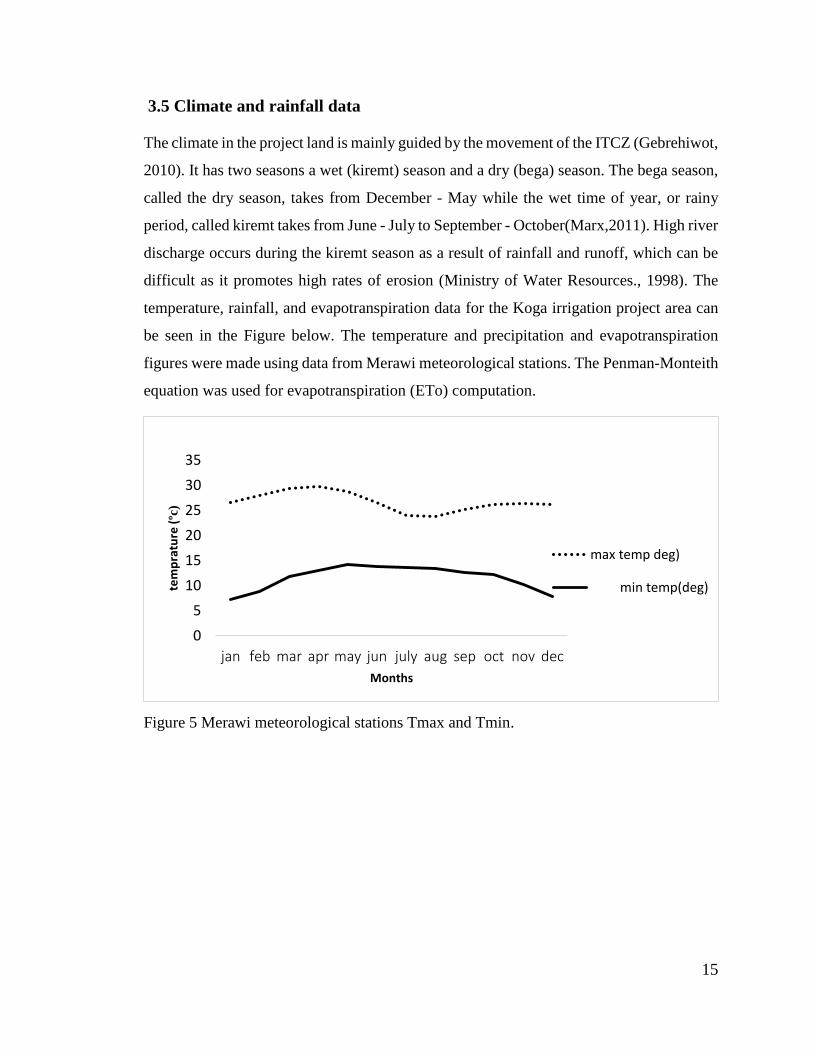
3.5 Climate and rainfall data
The climate in the project land is mainly guided by the movement of the ITCZ (Gebrehiwot,
2010). It has two seasons a wet (kiremt) season and a dry (bega) season. The bega season,
called the dry season, takes from December - May while the wet time of year, or rainy
period, called kiremt takes from June - July to September - October(Marx,2011). High river
discharge occurs during the kiremt season as a result of rainfall and runoff, which can be
difficult as it promotes high rates of erosion (Ministry of Water Resources., 1998). The
temperature, rainfall, and evapotranspiration data for the Koga irrigation project area can
be seen in the Figure below. The temperature and precipitation and evapotranspiration
figures were made using data from Merawi meteorological stations. The Penman-Monteith
equation was used for evapotranspiration (ETo) computation.
Figure 5 Merawi meteorological stations Tmax and Tmin.
0
5
10
15
20
25
30
35
jan feb mar apr may jun july aug sep oct nov dec
tem
pra
ture
(ºc
)
Months
max temp deg)
min temp(deg)

16
Figure 6 Merawi meteorological stations rainfall and eto.
3.6 The water balance Model and its components
The water balance model is a science and engineering rule such as applicable for protecting
the environmental role or improving the environmental benefits of a number of water
projects including irrigation, municipal water supply, and wastewater systems. The water
balance model, which calculates reservoir inputs and outputs, is another way of knowing
the hydrologic cycle and the feasibility of the reservoir cycle, as well as comparing the
supply volume of reservoir sustainability of sedimentation and climate change (Dingman,
2002). The water balance equation generally describes equating the balance between the
flowing input and output flow of any hydrological cycle. Due to the high degree of
complexity of our water process, they are always classified into independent components.
preparing a monthly water balance for the reservoir makes it possible to predict the supply
volume of the reservoir on a monthly basis. The water balance is designed to compare the
supply irrigation water volume of the reservoir with the crop water requirement in order
to estimate a final reservoir supply volume for a given month.
0
50
100
150
200
250
300
350
400
450
500
jan feb mar apr may jun july aug sep oct nov dec
rain
fal
l an
d e
to
month
rainfall and evapotranspiration
rain fall(mm/month)
eto(mm/month)

17
The model and equations used for calculating different parts of the water balance parameter
are described below. The water would be presented, along with a description of all of the
parameters and equations used to compute them. The parameters used in the reservoir
volume water balance model was computed in this section.
Vm= Vm-1 + p+ Qin) - (E + Qout). Equation 1
Equation 1 was taken For the Koga Reservoir because the water balance equation is used
for large reservoirs (with a volume of more than 50 Mm3). Put in a monthly time step as
much of the climate data used to calculate the parameter is given in monthly value. So my
project site is 83.1Mm3 which is greater than 50 Mm3 in a semiarid tropical region used by
(Guntner, 2004). Where Vm is the specific storage volume of the reservoir at the specific
month m,
P is precipitation,
Qin is the discharge from the Koga River into the reservoir,
E is evaporation and
Qout is the discharge out of the main irrigation canal and bottom outlet.
All parameters were given in millions of cubic meters (Mm3). The model computes the
volume of the reservoir for each month based on the volume of the last month add inputs
and subtract outputs of the month. Parameters in the model are the discharge from the Koga
River, precipitation, and runoff. Water losses from the reservoir were included evaporation
from the reservoir area, the water discharged into the primary irrigation canal, and water
flows through the bottom outlet for monthly environmental balanced flows and sediment
release. The change in reservoir volume from one month to the other is therefore equal to
Figure 7 Reservoir inflows and outflows; parameters for the water balance
model

18
the precipitation plus the discharge from the river subtract evaporation from the reservoir
area and discharge from the reservoir outlets. The water balance model take September as
the first month since Ethiopia is located to the south of the equator is which is the line of
the eastern hemisphere (east of Greenwich meridian) this is the beginning of the hydrologic
cycle for the Northern Hemisphere as given by the United States Geological Survey
(USGS, 2008).
Koga reservoir volumes beginnings in September and endings in August. The volume is
expressed in Mm3 for each value. The beginning volume in the model (Vm-1) is the volume
for September, taking October as the beginning computed volume. The model area was
chosen to be a maximum volume of 83.1 Mm3 and a minimum volume of dead storage
which is 3.9 Mm3. The increased reservoir volume is the point at which the water stage in
the reservoir higher than the height of the spillway, as given in the design reports( Mott
MacDonald, 2004).
The main parameter important for the equation was taken from the design reports done by
Mott MacDonald. Monthly values for precipitation (P) were given in mm. Estimated river
discharge (Qin) was also given in Mm3. Three parameters of Qout, environmental balanced
flows, and maintenance flow were given in Mm3 per month. Other parameters had taken
from the design reports were monthly climate data for crop water requirement and
evaporation (E) computation and a list of reservoir surface areas at particular reservoir
volumes curve used for making a volume to surface conversion equation to compute
evaporation from the reservoir.
3.6.1 River discharge Inflow (Qin)
The Koga River discharge is the only river entering into the reservoir. Direct discharge
value is not assessable for the inflow at the reservoir, but a gauging station is put on a
tributary of the river just side the reservoir that can be used. Monthly gauging discharge
values were listed in the design reports (Mott MacDonald, 2004). And are given in Fig 8
and the values are in appendix table A5.

19
Figure 8 Monthly Qin values used in the water balance model.
Assumptions
The river flow (Qin) was suggested to include all runoff from the watershed. The gauging
site from which the data obtained is only an estimate of the actual amount of discharge
flowing into the reservoir. As a result, the flow at the gauging site may vary from discharge
at the reservoir inlet. The river discharge values used in the water balance model are an
estimation of the best available information.
3.6.2 Rainfall (P)
Rainfall data were assessable for each month in Merawi meteorological station in mm. In
order to calculate the volume in cubic meters, the Rainfall was multiplied by the surface
area of the reservoir at max level. All Rainfall falling outside of this area is count as runoff,
which is added to river flow (Qin). When the reservoir is not at a full level due to
evaporation or water use, the surface area would be reduced. In spite of this, the area of the
reservoir at the full level is still used to determine the direct Rainfall falling on the reservoir.
This means the area used for computing the Rainfall input will be larger than the surface
area of the lake. As a result when the maximum volume, the Rainfall surface is equal to
the reservoir surface area plus the exposed land that would be included by the reservoir at
maximum level. This covered area would be incorporated into the runoff, although in order
to clear things the surface area is kept constant when calculating Rainfall. Monthly Rainfall
(P) values used in the water balance model are given in Figure 9 appendix A table A6.
0
5
10
15
20
25
30
35
40
Jan Feb Mar April May June July Aug Sep Oct Nov Dec
Qin
(Mm
3)
Months

20
Figure 9 Monthly Precipitation values used in the water balance model.
Assumptions
In computing the Rainfall input (P) it is suggested that all of the Rainfall falling on the
included area of the reservoir would make it into the reservoir as runoff. It is also suggested
that all runoff generated from Rainfall falling outside of the surface area of the reservoir at
a maximum level such as in the upstream watershed, is included in Qin.
3.6.3 Evaporation (E) of the Bahir Dar, Merawi, and Koga site
To compute the evaporation from the Koga project, the evaporation (Eo) from the
simplified Penman equation was multiplied by the surface area of the reservoir in
maximum capacity in order to get Mm3 evaporated.
Eo = (0.015 + 0.00042T + 10-6h) (0.8Rs-40 + 2.5F*u (T-Td) Equation 2
Where T is weighted air temperature in degrees Celsius, h is altitude in m, Rs is solar
radiation in w/m2, Td is the dew point temperature, F* is approximated as 1-8.7*10-5h, and
u is the wind speed in m/s. Weighted air temperature is used to estimate temperature from
the maximum (Tmax) and minimum (Tmin) temperature values. The equation for computing
weighted temperature is taken from Linacre (1993) and is given as:
T= (0.6Tmax+0.4Tmin) Equation 3
0
1
2
3
4
5
6
7
8
9
Jan Feb Mar April May June July Aug Sep Oct Nov Dec
P(M
m3)
Months

21
Dew point temperature would be calculated from relative humidity and air temperature
using the August-Roche-Magnus approximation (Equation 4)
Td = bG/a-G
Where G = (aT/b+T) + ln(RH/100) Equation 4
Where a is 17.271, b is 237.7 degrees Celsius, and RH is the relative humidity in %. The
output for the evaporation from the Koga project for each month in Mm3 is given in Figure
10. These are the result used in the water balance model when there has been a normal state
of the initial volume. New conversion curves were created and used to calculate new
monthly evaporation values for the scenarios suggesting a change in initial sediment.
Values for the evaporation in mm and Mm3 are given in Table A7 in Appendix A.
Figure 10 Monthly evaporation values used in the water balance model
Assumptions
The evaporation computation suggests a constant in the Koga reservoir’s area classification
throughout the time. Nevertheless, in actual the behavior of the reservoir concerning
evaporation would change as the depth in the reservoir changes. Therefore, It should be
0
0.5
1
1.5
2
2.5
3
3.5
Jan Feb Mar April May June July Aug Sep Oct Nov Dec
E (
Mm
3)
Months
Koga Reservoir

22
considered that these evaporation computations are predicted subject to huge margins of
error even though they are based on the best data and last research available. The computed
evaporation equation in mm (Ec) shows good results with the evapotranspiration (ET) data
from the Bahir Dar meteorological site.
3.6.3.1 Evaporation model scenario analysis
Comparing the computed evaporation for the Koga project, with the evapotranspiration
from Bahir Dar and merawi meteorological station, it can be seen that the output are similar
and follow the same monthly curve. This was true as Bahir Dar has a similar climate, found
just 35 km away from the Koga reservoir. The equation used to calculate evaporation
output is known as an assumption but the comparison did fit well, indicating the
calculations are consistent with observed values in the nearby Bahir Dar meteorological
station. To check the perfection of the computed evaporation for the Koga site, the values
were compared with data from the Bahir Dar meteorological station. The annual
evaporation in mm was calculated to be 1715.7, an equivalent of 24.4 Mm3. As a
comparison, the rainfall was predicted in the design report to be 1588.9mm yearly. The
month with the lowest evaporation in Mm3 is July and August, with a value of 1.7Mm3.
April is the month with the highest evaporation at 3.1 Mm3. These real evaporation values
for the reservoir depend not only on the evaporation rate but also on the shape of the
reservoir. Evaporation at the Koga reservoir and evapotranspiration in Bahir Dar
meteorological station, are compared in Figure 11. Monthly evapotranspiration values for
Bahir Dar meteorological site in mm, which is taken from the design report, are also
presented in Appendix A in Table A4.

23
Figure 11 Comparison of monthly Eto, Ecal, and Koga E of the site.
3.7 Outflow (Qout)
Discharge from the reservoir (Qout) can be classified into three different units; monthly
environmental compensation flows, maintenance flow, and irrigation flow. Monthly data
is assessed in the design report for environmental flow and maintenance flow, which occurs
only once annually. Climate data from the Merawi and Bahir Dar meteorological site and
the cropping patterns had given in the design reports were used for computing the irrigation
release.
3.7.1 Release discharge for Maintenance and sediment flushing
Maintenance flow occurs only once a year for sediment releasing taking 30 minutes, and
flushing 0.0558 Mm3 of water. This is a little significant compared with the other unit of
Qout. The maintenance flow is ordered for the month of June in the water balance model,
this means when the water level in the reservoir is low. Water can also be flushing for
maintenance than sediment releasing.
3.7.2 Environmental compensation flow
To see the possibility that in order to provide the irrigation water needed to supply the
whole command area the Koga project engineers were willing to neglect the environmental
compensation flow to compute sedimentation.
0
20
40
60
80
100
120
140
160
180
200
E(m
m)
month
koga E(mm)
KogaEcalc(mm)
BDR E(mm)

24
First, the reservoir volume was examined with decreasing volumes and under the
assumption that environmental release flows were only be shut off during the months where
the reservoir volume reaches a minimum.
Second, the reservoir volume is examined with change initial volumes and no
environmental flows released at the entire course of the year. Prioritizing the irrigation flow
over the environmentally balanced flows would advantage the farmers in the Koga
irrigation project area but would be respected by the downstream communities and
ecosystems as the water supply would be cut off. Stopping the environmental release is not
named in the design reports and is not likely to happen as a management activity in the
future for an ethical and legal case. However, the opportunity was examined for
theoretical/ideal/ purposes.
There is an actual amount of water that needs has to be flown into the downstream of the
Koga irrigation project area each month in order to respect natural flows in the Koga River
as they were before the Koga irrigation dam was built. In this way, it can be assured that
the downstream community will not be missing out on their water rights and the
downstream ecosystems can be protected. Turning off the environmental balanced release
during the months when the reservoir would run dry/ does not save enough water/ to irrigate
the whole project area using the current and future cropping pattern. Eliminating the
environmental balanced also becomes unable to supply sufficient water for irrigation after
the reservoir is forced to start operating at 78% maximum volume (Ministry of Water
Resources, 2006). The monthly Environmental compensation release was given in Figure
12 below

25
Figure 12 Water released from the reservoir for environmental compensation flow
for each month given in Mm3 (Ministry of Water Resources, 2006).
Figure 13 Water released reservoir for partial environmental compensation release
flow for each month given in Mm3 (Ministry of Water Resources, 2006).
As shown in Figure 12 and Figure 13 without affecting the downstream right I can redesign
the environmental compensation release flow and prolong the use full period of the
reservoir. As a result, shown above the redesign neither affecting the downstream nor the
reservoir.
0
0.5
1
1.5
2
2.5
3
month oct nov dec jan feb mar apr may
wat
er r
elea
se (
Mm
3)
Months
0
20
40
60
80
Sep Oct Nov Dec Jan Feb Mar April May June July Aug
wat
er r
elea
se (
Mm
3)
Months

26
3.7.3 Irrigation water release flow
3.7.3.1 Crop water demand (CWR) analysis
Nevertheless, this was not the final result used for the irrigation water flow parameters of
Qout, as there is no irrigation during the months of June-August. In order to check that the
policy of not irrigating during the peak of the wet season was realistic, I compared the
rainfall with the crop water demand for the three months in question. The wet season crop
pattern of 40% teff, 20% maize, 20% noug, and 20% millet give combined
evapotranspiration of about 27.95 Mm3 for the entire 7000 hectares of command area. For
the months of June-August, when there is no pattern irrigation, the combined evaporation
is 22.87 Mm3. Values for each month are given in Appendix A in Table A7. The rainfall
(Merawi extended rainfall values) falling on the command area’s 7000 ha during the rainy
season is 28.99 Mm3, for the combined months of June, July, and August. The precipitation
is therefore slightly larger than the total evapotranspiration during this season. If there is
no pattern irrigation during this period then the precipitation amount must fulfill the crop
water demand. The precipitation will meet crop water requirements if the efficiency of the
rain-fed irrigation is 79% (22.87Mm3/28.99Mm3) this shows the combined evaporation is
lower than the combined precipitation. It should be possible to operate using rain-fed
irrigation during June-August, nevertheless, if the whole project area is cropped during this
time, irrigation may not be needed to ensure crop survival.
The GIWR would vary based on the cropping patterns and irrigation schedule. Mott
MacDonald, therefore, estimated four different scenarios based on different climate data
and crop growing season lengths in order to generate different examples of possible gross
irrigation water demand. Total hectares of area irrigated each month vary between the
scenarios which affect the final yearly gross water requirement (GIWR).
Scenario I is dependent upon a short growing season and revised original climate data from
the working papers done by Mott MacDonald and has a predicted yearly GIWR of 60Mm3
(Ministry of Water Resources, 2006).
Scenario II uses the same data in conjunction with scenario I a longer growing season,
which has an estimated yearly GIWR of 76Mm3/yr.

27
Scenario III take a short growing season and wind speed data for evapotranspiration
computation from Bahir Dar, 30 km north of the site with a GIWR of 58Mm3/yr and
Scenario IV uses the same data in conjunction with scenario III but with a long growing
period, has an estimated yearly GIWR of 74Mm3/yr. These scenarios were estimated for
designing the dam and irrigation canals but none of them are being applied exactly in
practice today. Monthly values for each scenario as well as other details about the scenarios
are given in Table A14 in Appendix A. This comparison shows a tolerable difference
between the requirement (CIWR) design report result. So it is possible to use these data
enterchangebly for my thesis.
Figure 14 Comparison of crop irrigation water demand CIWR from the design
report scenarios
Assumption
The crop water demand computation is based on a few suggestions. These assumptions are
that the whole crops are planted at the same time, at the start of the respective planting day.
This is done in order to get the simplified result that well fits the water balance model on a
monthly respective time. In actual the crops are not all planted on the same day, they are
planted in different places on different days, always in rotations. For example, maize could
be planted on 4 different dates during the planting month, once at the starting of each week.
This prediction of water demand is therefore not perfect, but rather a monthly prediction
of water is needed. The computed crop water demand also assumes an irrigation efficiency
0
10
20
30
40
50
60
70
80
90
Oct Nov Dec Jan Feb Mar April May June July Aug Sep
CIW
R
month
Scenario IV(CIWR)
Scenario III(CIWR)
Scenario II(CIWR)
Scenario I(CIWR)

28
of 50% and are correspondingly computed as double the sum of the evapotranspiration for
each month.
3.7.4. Secondary data collection
Secondary data used for the study were collected as much as possible from responsible
bodies and officials. These data include discharge of the Koga River, climatic data, and
existed irrigation water requirements for the command area for the project. Discharge data
collected from the Ministry of Water Resources enclosed different stations on the Upper
Blue Nile basin.
3.7.5 Data analysis techniques
Data collected using different models, equations and techniques were analyzed and
interpreted as specific stated research objectives and study questions. A water balance
model that involves predictive sediment yield was used to analyze, interpret, and discussed.
Analysis and interpretation, preparatory works that involve data editing has been employed
in order to minimize irregularities and maximize accuracy by using medley software. To
this effect, physical data editing has been performed in order to see problems that made an
error, and data concentrated effort was the second task that I had employed as data collected
are subject to a series of check-ups in order to clean them from invalid formats, unusable
values and check the reasonableness of the distribution. The other preparatory task is data
Grammarly correction, where collected information is translated into values appropriate
for further data analysis, and types of variables representing the factors to be studied have
been identified, and given values/levels. To do this thesis I were used mendely softwear
for citation and bibliography, and grammarly checher.
3.8 Model scenarios
The Koga reservoir volume could reduce in the future mainly due to sedimentation and
climate change. I hope Sedimentation is occurred in the reservoir and knows about being a
harsh condition of the country. Draughts, minimum rainfall, and intense storms are capable
of reducing the reservoir’s volume, either by reducing the water demand from precipitation
and river runoff or by increasing sediment load and evaporation, this results an increase of
sedimentation in the reservoir.
If the sediment accumulation rates of reservoir 5 Mm3 every 7 years estimated in the design
reports by Mott MacDonald hold correct, this could mean the dam runs dry for at least one

29
or two months of the year ( Benjamin, 2013). In order to get an idea of how the reservoir
volume may change throughout a year under changed climate and sedimentation predicted
for the future, I created 4 scenarios
The reservoir volume decreases by 0 5, 10, and 15, Mm3 of sediment accumulation were
selected. These in turn correspond to new Vm-1 values of 83.1, 78.1, 73.1, and 68.1, Mm3.
The parameters in the water balance equation that were simplified in this scenario were the
extra several new Vm-1 equations were created. Monthly values for all of the model
component are presented in Appendix A in Tables A10.
3.8.1 Model Scenario 1
Computation from water balance equation, under 0 sediment acommulation. Figure 15
gives the normal state volume of the reservoir for a month as computed in the water balance
model or the volume reduction of the reservoir before 7 year as computed in the water
balance model. .
3.8.2 Model Scenario 2
Computation from water balance equation, under 5 Mm3 sediment acommulation. Figure
16 gives the volume reduction of the reservoir after 7 year as computed in the water balance
model.
3.8.3 Model Scenario 3
Computation from water balance equation, under 10 Mm3 sediment acommulation. Figure
17 gives the volume reduction of the reservoir after 14 year as computed in the water
balance model.
3.8.4 Model Scenario 4
Computation from water balance equation, under 15 Mm3 sediment acommulation. Figure
18 gives the volume reduction of the reservoir after 21 year as computed in the water
balance model.
The results from scenarios 1, 2, 3 , and 4, simulating possible upcoming reservoir volumes
change are presented below in figures 15-18.

30
4 Model scenarios Results and discussion
4.1 Model scenarios Results
In this part, the variability in volume of the reservoir throughout the period of a
hydrological year has resulted for each model scenario. The possible role of changes in
sedimentation on reservoir volume is discussed.
This volume decreases of reservoir by 0, 5, 10, and 15Mm3 due Sediment increase is in the
year of 2006, 2013, 2020, and 2027, respectively. These in turn correspond to new Vm-1
values of 83.1 78.1, 73.1, and 68.1Mm3.
4.1.1 Scenario 1 Reservoir volume under normal states
From Computation of water balance equation before 7 year sediment accumulation results
a minimum reservoir volume of 6.7Mm3 in may in 2006 E.C. The results from scenarios 1
simulating possible upcoming reservoir volumes are mentioned in figures 15.
4.1.2 Scenario 2 reservoir volume change by 5Mm3
Computation from water balance equation, under a 5Mm3 sediment accumulation or after
7 year sediment increase results a minimum reservoir volume of 4.8Mm3 in may in 2013
E.C. The results from scenarios 2 simulating possible upcoming reservoir volumes are
mentioned in figures 16.
0
20
40
60
80
100
Sep Oct Nov Dec Jan Feb Mar April May June July Aug
Volu
me(
Mm
3
Months
Before 7 years sediment accumulation
Figure 15 Reservoir volume under normal states

31
Figure 16 gives reservoir volume reduction by 5Mm3 for each month as computed
in the water balance model.
4.1.3 Scenario 3 reservoir volume change by 10 Mm3
From water balance equation Computation, under a 10Mm3 sediment accumulation or after
14 year sediment increase results a minimum reservoir volume of 2.9 Mm3 in may in 2020
E.C. The results from scenarios 3 simulating possible upcoming reservoir volumes are
mentioned in figures 17.
Figure 17 gives reservoir volume reduction by 10Mm3 for each month as
computed in the water balance model.
0
20
40
60
80
100
Sep Oct Nov Dec Jan Feb Mar April May June July Aug
Volu
me(
Mm
3)
Months
After 7 Years sediment accumulation
0
20
40
60
80
100
Sep Oct Nov Dec Jan Feb Mar April May June July AugVolu
me(
Mm
3
Months
After 14 years sediment accumulation

32
4.1.4 Scenario 4 reservoir volume change by 15 Mm3
Computation from water balance equation, under a 15Mm3 sediment accumulation or after
21 year sediment increase results a minimum reservoir volume of 0 in may in 2027 E.C.
The results from scenarios 4 simulating possible upcoming reservoir volumes are
mentioned in figures 18.
Figure 18 gives reservoir volume reduction by 15Mm3 for each month as
computed in the water balance model.
0
10
20
30
40
50
60
70
80
Sep Oct Nov Dec Jan Feb Mar April May June July Aug
Volu
me(
Mm
3
Months
After 21 years sediment accumulation

33
4.2 Model scenario Discussion
In this section:-
The results obtained in the last part are presented. The current and the future nature of the
Koga reservoir for the irrigation project is discussed,
The Koga reservoir volume could reduce in the future mainly due to sedimentation and
slight climate change. I hope Sedimentation is occurred in the reservoir and knows about
being a harsh area of the country. Water balance modeling to estimate an increase in
sedimentation direct to more water loss due to reservoir volume reduction and causing
more droughts and famine as well as minimum rainfall. Draughts, minimum rainfall, and
intense storms are capable of reducing the reservoir’s volume, either by reducing the water
demand from precipitation and river runoff or by increasing sediment load and evaporation,
resulting from an increase in dam sedimentation. The water balance model, not the only
model that the reservoir volume as it would behave under current climate conditions with
no reduction in maximum volume from sedimentation but also the future climate condition.
If the prediction of sedimentation yield of five Mm3 every seven years were true, the
reservoir would be depleted for at least part of the month in 2027 E.C. This tells us
decreases in the reservoir's maximum volume could create a huge problem for the reservoir
in the 21 years.
4.2.1 Model scenario 1 Reservoir volume under normal states
using current and future sedimentation results and unchanged in initial reservoir volume,
the reservoir should be able to feed sufficient water for irrigation and environmental
balance discharge throughout the month. The reservoir decreases a minimum volume of
6.7Mm3 in May. At this minimum volume, the reservoir is not in the problem of being
irrigating the entire command area and has sufficient flow to supply additional irrigation
area. The minimum result appears just the end of the winter season as this is the time of
year when the reservoir has been in the largest use. As the wet season starts, the reservoir
is no longer used for irrigating and starting instead it overfill. The reservoir is able to
overfill to a huge volume than the beginning volume. The entire course of the hydrological
year, the reservoir volume enhances 13.1Mm3 in size, make full to its maximum volume.

34
Even though, it has the capacity of irrigating the entire command areas. However, it might
not always be able to irrigate this in the future as sedimentation and changes in climate
become increase. Scenarios 1-4 give susceptible outcomes for Koga reservoir volumes in
the future and remedial measures/mitigation action/.
A 0 sediment accumulation in reservoir volume directs to the Koga reservoir just sufficient
to supply already in May and after a reservoir becomes 13.1Mm3 in June.
The graph shows the reservoir is longer able to feed sufficient water for the year, in May,
becoming close to the reservoir. The reservoir is still able to feed water year over
nevertheless, it reaches a minimum volume of 6.7 Mm3 it seems to good to irrigate.
4.2.2 Model Scenario 2 reservoir volume change by 5Mm3
In 5Mm3 reservoir volume reduction, by using future sedimentation result with the 2013
E.C year reduction in initial reservoir volume. Nevertheless, the reservoir should be able
to give sufficient water for the whole command area and possible to release environmental
compensation flow the entire year. The reservoir decreases a minimum volume of 4.8Mm3
in May. At this minimum volume, the reservoir is not in the problem of being irrigating the
entire command area and has sufficient flow tosupply additional irrigation area. The
reservoir is able to overfill to a huge volume than the beginning volume. During the entire
course of the hydrological year, the reservoir volume enhances 8.1Mm3 in size, make full
0
10
20
30
40
50
60
70
80
90
Sep Oct Nov Dec Jan Feb Mar April May June July Aug
Vo
lum
e( M
m3)
Months
Figure 19 Reservoir volume under normal state

35
to its maximum volume. Even though, it has the capacity of irrigating the entire command
areas. However, it might not always be able to irrigate this in the future as sedimentation
and changes in climate become increase. Scenarios 2-4 give susceptible outcomes for Koga
reservoir volumes in the future and remedial measures/mitigation action/.
Figure 20 Reservoir volume by 5Mm3 reduction
The graph shows the reservoir is longer able to feed sufficient water for the year, in May,
becoming close to the reservoir. But the reservoir is still able to supply water year over
nevertheless, it reaches a minimum volume of 4.8 Mm3 again it seems to good to irrigate
A 5Mm3 decrease in maximum volume directs to the Koga reservoir just becoming
minimum already in May and after the reservoir becomes 8.1Mm3 in June.
4.2.3 Model Scenario 3 reservoir volume change by 10Mm3
The graph shows the reservoir is longer able to feed sufficient water for the year, in May,
becoming close to the reservoir. The reservoir is still able to supply water year over
nevertheless, it reaches a minimum volume of 2.9 Mm3 again it seems to good to irrigate.
In 10Mm3 reservoir volume reduction, by using future sedimentation result with the
2020E.C year reduction in initial reservoir volume. Nevertheless, the reservoir should be
able to give sufficient water for the whole command area and possible to release
environmental compensation flow the entire year. The reservoir decreases a minimum
volume of 2.9Mm3 in May. At this minimum volume, the reservoir is not in the problem
0
10
20
30
40
50
60
70
80
90
Sep Oct Nov Dec Jan Feb Mar April May June July Aug
Vo
lum
e( M
m3)
Months

36
of being irrigating the entire command area and has sufficient flow to supply additional
irrigation area. The reservoir is able to overfill to a huge volume than the beginning volume
by10.3Mm3in June. Even though, it has the capacity of irrigating the entire command areas.
However, it might not always be able to irrigate this in the future as sedimentation and
changes in climate become increase. Scenarios 3-4 give susceptible outcomes for Koga
reservoir volumes in the future and remedial measures/mitigation action/.
A 10Mm3 decrease in maximum volume directs to the Koga reservoir just becoming
minimum already in May and after that, the reservoir becomes 10.3Mm3 in June.
Figure 21 volume reductions Reservoir by 10 Mm3.
4.2.4 Scenario 4 reservoir volume change by 15Mm3
In 15Mm3 reservoir volume reduction, by using future sedimentation result with the 2027
E.C year reduction in initial reservoir volume. Nevertheless, the reservoir should not be
able to give sufficient water for the whole command area, and impossible to release full
environmental compensation flow the entire year. At this minimum volume, the reservoir
is in the problem of being irrigating the entire command area and has an insufficient flow
to supply additional irrigation area. The reservoir is able to overfill to a huge volume than
the beginning volume by 7.5Mm3 in June. Therefore, it has not the capacity of irrigating
0
10
20
30
40
50
60
70
80
90
Sep Oct Nov Dec Jan Feb Mar April May June July Aug
Vo
lum
e( M
m3
Months

37
the entire command areas. Scenarios 4-4 give susceptible outcomes for Koga reservoir
volumes in the future. A 15Mm3 decrease in maximum volume directs to the Koga reservoir
just becoming empty already in May and after that, the reservoir becomes 7.5Mm3 in June.
4.2.5 Model scenario summary
When I summarise ize the four different scenarios for reservoir volume change discussed
in the calculation result obtained and described in the previous section, the calculated
reservoir volume change is roughly varied due to the number of reduction terms of volume
and greatly varied From year to year. This can be shown in Figure 23.
Figure 23 Scenario 1-4: shows Changes in reservoir volume with decreases in the
maximum volume due to sedimentation. Different decreases in the maximum volume are
given, ranging from no decrease to a 15Mm3 decrease in the initial reservoir volume.
Figure 24 displays the volumes calculated for each month in scenarios 1-4, using reduced
initial reservoir volumes to simulate sedimentation. The dam volume reaches zero in the
model runs with reductions in initial reservoir volume of 15Mm3 and greater than this. This
tells Sediment increase reservoir volume decrease
0
10
20
30
40
50
60
70
80
Sep Oct Nov Dec Jan Feb Mar April May June July Aug
Vo
lum
e( M
m3)
Months
Figure 22 Reservoir volume by 15Mm3 reduction

38
Figure 23 summary of volume change due sediment accumulation in different year
from scenario 1-4
0
10
20
30
40
50
60
70
80
90
Sep Oct Nov Dec Jan Feb Mar April May June July Aug
volu
me(
Mm
3 )
month
summary
2006 E.C
2013 E.C
2020 E.C
2027 E.C

39
5. Conclusion and recommendation
5.1 Conclusion
The following conclusions were listed after computing the change in reservoir
sedimentation based on the water balance model. The thesis first analyzed the sediment
variability, volume capacity loss, useful lifetime, and amount of deposited sediment over
its useful time in the Koga irrigation project. The water balance model requires several
parameters, such as Koga River inflow (Qin) the precipitation, evaporation, and the outflow
(Qout) of the reservoir.
In this study, the investigation of the change reservoir sedimentation was done through the
method of water balance equation. The main problem during my thesis was to know the
reservoir size every year to calculate precipitation and evaporation due to this difficulty I
did the reservoir size constant which could lead to huge errors. Therefore, in the future, the
Koga irrigation project engineer should consider the change in reservoir size.
According to the water balance model, the Koga reservoir should be able to feed sufficient
water for irrigating the whole project area up to 10Mm3 sedimentation deposition. The
reservoir is able to come up to maximum volume at the end of the hydrologic month in
four scenarios but scenario four did not do like others. Due to this, the future of the project
is threatened by the problem of sedimentation. The model result tells that after a 15 Mm3
reduction in initial volume the reservoir becomes dry for at least one month of the year.
The Koga irrigation project office aims to increase the number of command areas in the
future. If sedimentation happens, the reservoir supply volume will most likely be reduced
below the volume required to irrigate 7000 ha. If the reservoir fails to supply the required
volume for the project design, the dam could be considered a failure and might affect the
farmer’s interest. Not only farmers in the irrigable land affected, but also for the rest of
Ethiopia.
However, sedimentation increase had the greatest effect on reservoir volume this causes
large decreases in reservoir volume throughout the year and the model showed the dam
running empty.

40
Generally, the results of the model could use as an important origin to support the design
and implementation of sediment protection policy in the catchment area and deposition in
the Koga reservoir.
5.2 Recommendations
Based on the water balance studies and result the following recommendations were
suggested. Nevertheless, comparing the result of sediment rate and useful life/design period
of the reservoir with the design document was not formulated. There are so many active
gullies on the catchment area as observed in the study shows. These gullies have much
depth and width eroded simply by the flood. Therefore, it is very useful to treat these gullies
to decrease the inflow sediment and expand the life span of the dam. Irrigational farmland
near the reservoir is plowed around to the reservoir area on both sides of the reservoir.
Therefore, this practice maximizes the sediment deposition to the reservoir, then decrease
the incoming sediment and expand the life span of the reservoir. Engineers, Designers,
managers, and decision-makers should give attention to installing adequate bottom outlets
for sediment discharge/flushing deposited sediments /or sluice get by considering the
amount of sediment releasing from the reservoir on catchment designing in order to
maximize the useful life of the reservoir.
Generally, this study work in the Koga irrigation project has been performed by water
balance model and can provide some methodological benefit for other catchment studies
in the area. Koga irrigation scheme suffers from economic water scarcity that makes its
water utilization difficult. A detailed understanding of the hydrological processes is
important for balancing crop irrigation water requirement and the reservoir volume. And
this type of study has to be adopted and accomplished on some other irrigation projects in
the country. Hydrologic analysis, the 80% dependable flow of Koga River indefinite dry
years did not meet the Crop Water Requirement. For that reason, to take care of the
uncertainties, mechanisms such as increasing storage in the catchment in a form of a pond
and small dams, reduction of command area when demand is greater than the available
discharge in the river, adopting time management for irrigation means irrigating crops at
night, morning and evening is best and also the provision of night storage is important.

41
6. Reference
Alemaw, D., Ayana, E. K., Legesse, E. S., Michael, M., Tilahun, S. A., & Moges, M.
A. (2016). Estimating reservoir sedimentation using bathymetric differencing and
hydrologic modeling in data-scarce Koga watershed, Upper Blue Nile, Ethiopia.
110(2), 413–427. https://doi.org/10.12895/jaeid.20162.519
Britannica. (2010). Britannica Online Encyclopedia, available
Benjamin. (2013). Variability and change in Koga reservoir volume, Blue Nile, Ethiopia
CIAWorld Fact Book ( (2012). Available at: https://www.cia.gov/library/publications/the-
world-factbook/geos/et.html, Accessed 2012. 31(2), 3245.
Clothier. (1993). B. E., Green, S. R. Rootzone Processes and the efficient use of irrigation
water, Environment Group, Hort Research, Private Bag 11-030, Palmerston North,
New Zealand.
Dingman. (2002). Physical Hydrology. 2nd ed. New Jersey: Prentice-Hall.
Eguavoen. (2011). I., Weyni T. Rebuilding livelihoods after dam-induced relocation in
Koga, Blue Nile basin, Ethiopia, ZEF Working Paper 83. Bonn. August.
https://doi.org/10.21276/ijee.2017.10.0305
Guntner. (2004). Krol, M. S., De Araujo, J. C., Bronstert, A., Simple water balance
modeling of surface reservoir systems in a large data-scarce semiarid region,
Hydrological Sciences– Journal–des Sciences Hydrologiques, 49.
H.M.Raghunath. (2006). Hydrology, New Age International (P) Limited, Publisher New
Delhi.
Habtom. (2009). Evaluation of Climate Change Impact on Upper Blue Nile Basin
Reservoir. 9(8).
IPCC. (2001). The scientific basis technical summary of the working group I report.
Cambridge university press, New York, 94pp.
IPCC. (2007). Technical paper VI Climate change and Water.
Kenneth. (1997). Frederick, Senior, F. Water Resources and Climate Change, Washington,
DC. January. https://doi.org/10.1017/S0014479710000955
Marx. (2011). Large-Scale Irrigation in the Blue Nile Basin: Changes and Obstacles in
Implementing Farmers’ Self-Management a Case Study of the Koga Irrigation and
Watershed Management Project in Amhara Region, Ethiopia, Research report for the
project.
Ministry of Water Resources. (1998). Abbay river basin integrated development master
plan project. In: Phase 2: data collection- site investigation survey and analysis.
BECOM (French Engineering Consultants) in association with BRGM and ISL
Consulting Engineer, Addis Ababa, Ethiopia.
Ministry of Water Resources. (2004a). Koga Irrigation Project Working Paper Nr. 1-10,
Available as a hardcopy at Koga Irrigation Project Office in Merawi. February.
Ministry of Water Resources. (2004b). Koga Irrigation Project Working Paper Nr. 1-10,

42
Available as a hardcopy at Koga Irrigation Project Office in Merawi.
Ministry of Water Resources. (2006). Koga Dam and Irrigation Project Design Report,
available as a hardcopy at Koga Irrigation Project Office in Merawi. 10(4), 269–280.
https://doi.org/10.5897/AJAR2014.8703
Ministry of Water Resources. (2008). Large-Scale Irrigation in the Blue Nile Basin:
Changes and Obstacles in Implementing Farmers’ Self-Management a Case Study of
the Koga Irrigation and Watershed Management Project in Amhara Region, Ethiopia,
Research report for the project. 127–155.
moges. (2010). Moges, Semu, Helmut Kloos, Stuart McFeeters and Worku Legesse (2010),
The Water Resources of Ethiopia and Large-scale Hydropower and Irrigation
Development, in Kloos, H. et al. (eds.) Water Resources Management in Ethiopia.
Mott MacDonald. (2004). Koga Dam and Irrigation Project Contract KDIP 3: Koga
Irrigation and Drainage System, Hydrology Factual Report. Available as a hardcopy
at Koga Irrigation Project Office in Merawi.
UNEP. (2000). Climate Change and Dams: An Analysis of the Linkages between the
UNFCCC Legal Regime and Dams, available
at:1www.dams.org/docs/kbase/contrib/env253.pdf, Accessed 15-08-2015. 6(1), 1–11.
UNESCO. (2004). United Nations Educational, Scientific, and Cultural Organization
World Water Assessment Program. 153–162.
USGS. (2000). Irrigation Techniques, Available at
http://ga.water.usgs.gov/edu/irmethods.html, Accessed 2012.
USGS. (2008). Explanations for the Natural Water Conditions, Available at
http://water.usgs.gov/nwc/explain_data.html.
vorosmarty. (1997). The storage and aging of continental runoff in large reservoir systems
of the world.
Wahaj. (2007). Policy Research Working Paper 4288: Actual Crop Water Use in Project
Countries: A Synthesis at the Regional Level, The World Bank Development Research
Group Sustainable Rural and Urban Development Team.

60
7. Appendix
Appendix A
Table A1 suggested cropping plan for the wet and dry season (Ministry of Water Resources, 2006)
Crop potato maize shallots peppers wheat millet noug teff sum
Dry season
(%)
16 47 12 7 18 100
Wet
season (%)
20 20 20 20 100
Table A2 Actual cropping pattern for dry season (Ministry of Water Resources, 2006).
Crop whe
at
barel
y
mai
ze
bea
n
Haricotbe
en
abis
h
fasol
ia
potat
o
cabba
ge
toma
to
carr
ot
beatro
ot
garl
ic
onio
n
preenpep
per
dry(
%)
31.4 19.6 3.23 0.2 0.10
8
0.0
1
0.00
5
41.6 0.55 0.229 0.00
1
0.00
4
1.22 1.38 0.60
1
Table A3 dry season proposed cropping system (%)
potato maize shallote peppers wheat
16 46 12 7 18

61
Table A4. Reservoir simulation runs. PIA is the potential irrigated area in hectares (Ministry of Water Resources, 2006)
Exp No. PIA (ha)
1 5833
2 5879
3 6104
4 6332
5 7588
6 7331
7 6143
8 6481
9 7645
10 7318
Table A5. Command Areas and their Sizes (Ministry of Water Resources, 2006). The addition of the Tekel Dib
extension area is designed for the future.

62
Table A6 Comparison of monthly evaporation between Bahir Dar meteorological station, calculated and the Koga site.
Month Jan Feb Mar April May June July Aug Sep Oct Nov Dec
BDR Eto(mm) 124 126.6 160.27 164.4 150.36 123 102.6 100.8 111.6 125.55 117.3 114.1
KogaEcalc(mm) 136 141.8 169.54 175.75 158.12 125.19 99.35 92.49 112.72 135.36 127.2 128.7
kaga E(mm) 138 141.4 173.86 178.23 156.58 123.86 98.04 95.38 114.27 137.41 131.5 129.2
koga E(Mm3) 2.41 2.47 3.04 3.11 2.74 2.16 1.71 1.67 2 2.4 2.3 2.26
Table A7 Data for Koga river inflow given by design reports Nile (Mott MacDonald, 2004)
Month Jan Feb Mar April May June July Aug Sep Oct Nov Dec
Qin(Mm3) 2.71 2.13 2.15 2.12 2.61 5.09 24.93 35.74 22.58 9.79 4.95 3.52
Table A8. Precipitation data for Bahir Dar (Ministry of Water Resources, 2004).
Month Jan Feb Mar April May June July Aug Sep Oct Nov Dec
p(mm) 3.2 1.7 10.1 30.6 102.7 227.8 445.3 406.7 219.7 102.2 23 5.3

63
p(Mm3) 0.06 0.03 0.17 0.53 1.79 3.98 7.79 7.11 3.84 1.78 0.43 0.09
Table A9 Crop Water Usage Values estimated by Mott MacDonald in the project report
Month Jan Feb Mar April May June July Aug Sep Oct Nov Dec
CIWR(Mm3) 9.95 6.72 3.44 0 3.89 7.08 10.3 6.07 1.61 0 4.14 7.72
CIWR*50% 19.9 13.43 6.88 0 7.79 14.2 20.05 12.14 3.21 0 8.29 15.45
Table A10 these different scenarios modify the variables in the water balance equation to represent changes in
sedimentation.
Month Sep Oct Nov Dec Jan Feb Mar April May June July Aug
V@0(Mm3) 83.1 79.4 80.9 53.7 32.5 21.8 11.3 11.1 6.7 13.1 55.3 80.1
V@5(Mm3) 78.1 76.9 69.4 56.3 29.7 17.5 8.9 8.8 4.8 8.1 44.3 72.7
V@10(Mm3) 73.1 72.3 64.5 49.7 27.1 15.4 6.2 6.1 2.9 10.3 45.3 70.1
V@15(Mm3) 68.1 67.6 61.9 48.3 29.1 26.4 3.1 3 0 7.5 46.1 69.8

64
Table A11 these different scenarios modify the variables in the water balance equation to represent the partial
environmental release.
month Sep Oct Nov Dec Jan Feb Mar April May June July Aug
V0.5
(Mm3)
73.1 67.6 61.9 48.3 29.1 26.4 3.1 3 0.5 7.5 46.1 69.8
Table A12. Monthly compensation flows (Ministry of Water Resources, 2006).
Month volume(Mm3)
Oct 2.68
Nov 1.56
Dec 0.8
Jan 1.07
Feb 0.97
mar 0.8
Apr 0.67
may 0.8

65
Table A13 Data for Crop Water Usage Calculations (Ministry of Water Resources, 2006)
crop crowing season length (days) ET(kc*Eto)(mm/day) ET(mm/season) dry area wet area
initial development mid end initial mid end % ha % ha
tomato 30 40 40 25 2.5 5 3.75 506.66 0.23 16.02 0
maize 25 40 45 35 1.3 5 2.5 469.13 3.23 226.2 20 1400
onion 5 25 40 30 2.9 4 4.17 395.11 1.38 96.46 0
garlic 5 25 40 30 2.9 4 2.92 357.58 1.22 85.06 0
potato 30 40 50 30 2.1 5 3.13 533.76 41.56 2909.1 0
Greenpeper 25 35 40 20 2.5 4 3.75 433.16 0.6 42.07 0
wheat 20 30 50 30 1.3 5 1.67 405.53 31.37 2195.9 0
barley 20 30 50 30 1.3 5 1.04 386.77 19.57 1369.6 0
beans 15 25 25 10 1.7 5 1.46 240.3 0.17 12.21 0
Haricotbeens 15 25 25 20 1.7 5 2.29 271.57 0.11 7.54 0
abish 15 25 25 20 1.7 5 2.29 271.57 0.01 0.74 0
fasilia 15 60 25 20 1.7 5 2.29 271.57 0 0.34 0
cabbage 40 30 50 15 2.9 4 3.96 614.03 0.55 38.53 0
carrot 20 30 40 20 2.9 4 3.96 422.21 0 0.08 0
beatroot 25 30 25 10 2.1 4 3.96 298.16 0 0.26 0
teff 20 30 45 25 1.3 5 1.67 373.22 0 40 2800
shallots 5 25 40 30 2.9 4 3.96 399.8 0 0
noug 25 40 50 30 1.5 5 1.46 445.15 0 20 1400
millet 20 30 55 40 1.3 4 1.25 385.73 20 1400

67
Table A14 Scenarios I-IV net irrigable are and. GIWR of the whole irrigated area (Ministry of Water Resources, 2008).
The scenario I; Revised climate data and cropping pattern with short period growing
varieties
month Jan Feb Mar April May June July Aug Sep Oct Nov Dec total
Net irrigable area 5897 7000 6988 4874 2380 5261 6930 7000 6988 4736 1246 4615
GIWR(Mm3) 12.38 12.4 19.27 7.6 0.87 0 0 0 1.15 2.91 0.36 2.58 60
Scenario II; Revised climate data and cropping pattern with long period growing
varieties
Net irrigable area 5306 6811 7000 6370 3090 5460 7000 7000 7000 7000 4302 3015
GIWR(Mm3) 8.17 11.52 20.15 13.94 1.42 0 0 0 2.85 11.76 4.1 1.19 76
Scenario III; Revised climate data and cropping pattern with short period growing varieties using Bahir Dar wind speed
data
Net irrigable area 5897 7000 6988 4874 2380 5261 4641 7000 6988 4736 1246 4615
GIWR(Mm3) 11.96 11.95 18.6 7.36 0.84 0 0 0 1.08 2.85 0.36 2.5 58
Scenario IV; Revised climate data and cropping pattern with long period growing varieties using Bahir Dar wind speed
data
Net irrigable area 5729 7000 7000 6370 3090 5460 7000 7000 7000 7000 4302 3028
GIWR(Mm3) 9.08 11.41 19.44 13.51 1.36 0 0 0 2.76 11.56 4.01 1.15 74

69
Table A15 Growing season lengths in months and total irrigation water
requirements in mm for selected crops as estimated by
crop water needed(mm) growing
season(month)
wheat 450-650 4 to 5
teff 400-600 3 to 4
maize 600-1200 4 to 5
barley 400=800 4 to 6
noug 80-1100 4 to 5
sweet
potato
500-1000 4 to 5
peppert 600-900 3 to 5
tomato 400-600 3 to 5
Table 16 Area covered by each crop
Crop type Barley Beans Maize Peppers Vegetab
le
Wheat Total
Area
covered
(ha)
157.5 9.9 538.7 53.4 2196 2750 5705

70
Table 17 Average monthly crop water requirement of cultivated crops in the
project
CWR(m3/s) Average Monthly
Total
Month Barley beans
Maize Pepper Vegetable Wheat Average
Jan 0.077 0.005 0.20 0.034 1.70 0.87 2.89
Feb 0.20 0.012 0.59 0.050 2.50
2.40 5.75
Mar 0.23 0.014 0.81 0.070 2.88 3.96 7.97
Apr 0.15 0.007 0.65 0.073 0.94 3.52 5.34
May 0.00 0.000 0.10 0.022 0.00 0.54 0.66
Total 0.66 0.038 2.35 0.250 8.00 11.29 22.58