The Impact of Rebuilding Grants and Wage Subsidies on the Resettlement

Choices of Hurricane Katrina Victims∗

Jesse Gregory

University of Michigan

jessgreg@umich.edu

Job Market Paper

November, 2011

Abstract

Following Hurricane Katrina, the Louisiana Road Home program provided cash grants di-rectly to individual homeowners to offset repair costs and to encourage rebuilding. I developa dynamic discrete choice model of New Orleans homeowners’ post-Katrina choices regardingresidential locations, home repairs, home sales, and amounts to borrow or save, and I deriveand implement a maximum likelihood estimator for the model’s structural parameters. Usingsimulations I find that the Road Home program significantly increased the fraction of homesrebuilt within four years of Katrina, mostly by relaxing financing constraints for householdsthat strongly preferred to rebuild. I find that location preferences are highly heterogenous, andmost households are far enough from the margin with respect to their preferred location thateven large location subsidies induce few households to change locations. These findings suggestthat disaster-related subsidies to dangerous locations generate substantially smaller economicdistortions than would be predicted by spatial equilibrium models with homogeneous agents.

∗I am grateful to David Albouy, John Bound, Charlie Brown, Brad Hershbein, Fabian Lange, Mike McWilliams,Morgen Miller, Narayan Sastry, Kevin Stange and seminar participants at the University of Michigan, MichiganState/Western Ontario/Michigan “Labor Day”, and the Population Association of America 2011 meetings for helpfulsuggestions. All remaining errors are my own. This work has been supported in part by a grant from the NationalPoverty Center at the University of Michigan, which is supported by award #1 U01 AE000002-03 from the U.S.Department of Health and Human Services, Office of the Assistant Secretary for Planning and Evaluation. Anyopinions expressed are those of the author alone and should not be construed as representing the opinions or policyof any agency of the Federal Government.

1 Introduction

Policymakers designing disaster relief packages face a difficult tradeoff. The desire to assist disaster

victims must be weighed against the fear that subsidizing people to live in dangerous areas will

generate moral hazard with regard to subsequent location decisions. The size of the economic

distortion caused by this type of moral hazard depends on the extent to which individuals’ and

households’ location choices are influenced by financial incentives. If each household is nearly

indifferent between many different residence locations, then disaster policies that subsidize residence

in a particular location will generate large distortions. If most households strictly prefer one

location, then it is possible for disaster relief programs to increase the welfare of residents in disaster-

affected areas without generating large distortions. A full appraisal of the impact of disaster-relief

policy on social welfare must consider the direct impact of disaster relief on victims’ welfare and

the extent to which the programs distort individuals’ location decisions.

This paper develops and estimates a dynamic discrete choice model of New Orleans homeown-

ers’ post-Hurricane Katrina resettlement choices. In the model, households make choices regarding

residential locations, home repairs, home sales, and amounts to borrow or save. The model’s pa-

rameters describe households’ preferences over consumption and residence locations and describe

households’ ability to borrow. The model is identified by variation across households in the finan-

cial incentive to rebuild provided by the Louisiana Road Home rebuilding grant program and by

variation in the relative labor wages available in New Orleans versus away from New Orleans for

workers in different occupations. I use the estimated model to measure the impact of post-Katrina

relief programs on households’ short term resettlement choices and to quantify a key component of

the deadweight loss associated with a guarantee of future relief.

The estimated model finds that households in this population have a strong preference for

living in New Orleans on average; there is substantial variation across households in the strength

of that location preference; and large population subgroups face borrowing constraints. The model

finds that the government’s Road Home program, which paid cash rebuilding grants to individual

homeowners, increased the fraction of homes rebuilt during the first four years following Katrina by

11%. This impact occurred primarily by relaxing borrowing constraints for households that would

have strongly preferred to rebuild even in the absence of the subsidy if the associated costs could

have been smoothed.

Estimates suggest that heterogeneity in location preferences is substantial enough that most

households are far from the margin with respect to their preferred location. This pattern implies

that the elasticity of location choices with respect to financial incentives is low, as few households

1

switch locations in response to a location subsidy. For this reason, simulations find that a guarantee

of relief in the event of a future disaster generates a deadweight loss that is small relative to the

policy’s expected cost.

Several recent studies have estimated explicit dynamic behavioral models to measure the re-

sponsiveness of migration choices to financial incentives. Kennan and Walker (2011) estimate a

dynamic discrete choice model of optimal migration and find that labor flows are responsive to

variation in wages across space. Several related studies have considered variations on Kennan and

Walker’s model to investigate particular aspects of migration.1 This paper contributes to that

literature in several important ways. This paper is the first to estimate a dynamic structural model

of migration that explicitly includes the asset accumulation choice and allows for the possibility of

borrowing constraints. Borrowing constraints will affect the migration choices of any population

that faces large up-front costs to moving. In the disaster context, those costs reflect the price of

home repairs. The model would be equally well-suited to investigate migration choices, for example,

among homeowners with negative mortgage equity, or other populations that face up-front costs

to moving. This paper also contributes to this literature by estimating a dynamic structural mi-

gration model using directly observable sources of variation in location-specific financial incentives.

Other studies in this literature have relied heavily on variation in the individual-location match

component of workers’ wages, which must be inferred statistically from panel wage data, to identify

the influence of earnings opportunities on migration. Because I replicate several key findings of

the existing literature using a different and more transparent source of identification, my study

provides an out-of-sample validation for the main conclusions of the existing literature.

The responsiveness of individual migration choices to financial incentives is of general interest

beyond the disaster-policy context. For example, the manner in which local or regional labor

markets adjust to labor demand shocks depends critically on the willingness of affected workers to

relocate (Blanchard and Katz, 1992; Bound and Holzer, 2000).2 If workers’ location choices are

not strongly influenced by financial incentives, then localized labor demand shocks will have large

wage effects that persist until capital re-adjusts. If workers quickly relocate in response to financial

incentives, then localized labor demand shocks will have short lasting wage effects and larger effects

on the size of local populations.

The responsiveness of individual migration choices to financial incentives also figures promi-

nently in the broader literature that examines the economic distortions caused by place-based

policies. If, as in classic models of spatial equilibrium (Rosen, 1979; Roback, 1982), workers are

1Gemici (2011) develops a model in which married couples must consider the potential labor earnings of both householdmembers across locations. Bishop (2007) applies a computational innovation that allows her to model migrationwith enough geographic detail that migration choices become informative about preferences for spatially delineatedamenities.

2Blanchard and Katz (1992) consider a model in which fully mobile (in the long run) workers and firms arbitrage awayshocks to local employment and wages, and the long-run employment effects of such shocks depend on the relativespeed with which workers and firms relocate. Bound and Holzer (2000) consider differences across race, education,and experience subgroups in the impact of labor demand shocks on wages, focusing on differences across groups inthe elasticity of migration with respect to financial incentives as the primary explanation for these differences.

2

fully mobile and share homogeneous location preferences, the deadweight loss associated with a

tax or subsidy to a given location depends entirely on the elasticities of local labor demand and

local housing supply (Albouy, 2009). Because long-run labor demand and housing supply are quite

elastic, this sort of model suggests that local policies generate large distortions. On the other

hand, if workers’ preferences for locations are heterogeneous, then the long-run supply elasticity of

residents to locations is finite (Moretti, 2011; Busso, Gregory, and Kline 2011), and local policies

will generate smaller distortions.

Finally, this study contributes to the literature that examines the economic consequences of

disasters and the more narrow literature that has examined patterns of post-Katrina migration and

resettlement.3 Hurricane Katrina struck the Gulf Coast of the United States on August 29, 2005 and

generated, in the years following, the largest disaster-relief effort in the nation’s history. The city of

New Orleans received some of the storm’s most concentrated and costly damage when, in the days

following the storm, the city’s protective levees failed and flood waters covered large areas of the

city. Government disaster relief to New Orleans following Hurricane Katrina included substantial

compensation packages to individual homeowners, in addition to traditional public disaster relief

services such as debris removal and infrastructure repair. Much of the Gulf Coast, including New

Orleans, was declared a federal disaster area in Katrina’s aftermath. This declaration immediately

makes available several standing federal disaster-relief programs that assist individuals directly.

Most notably, the Federal Emergency Management Agency provides small Disaster Assistance

Grants, and the U.S. Small Business Administration provides subsidized disaster assistance loans

to some homeowners.

Congress typically funds additional relief using supplemental appropriations when severe dis-

asters occur, and Congress funded several post-Katrina programs in this manner. A block grant4

to the state of Louisiana funded a large-scale rebuilding grant program known as the Road Home

program. The Road Home program paid grants of up to $150,000 directly to individual homeowners

to offset any repair costs not covered by insurance and was advertised as the largest single hous-

ing recovery program in U.S. history. The program provided smaller net compensation packages

to households that chose not to rebuild, thus providing an explicit financial incentive to rebuild.

Most Road Home grants were not paid until more than two years after Hurricane Katrina, but,

despite the program’s slow rollout, the Road Home program provided substantial compensation to

more than half of New Orleans households that owned homes rendered uninhabitable by Hurricane

Katrina.

Using the fitted model, I conduct simulation experiments to estimate the impact of the Road

Home rebuilding grant program on households’ resettlement choices. I find that the Road Home

program’s impact varied considerably across population subgroups. The program increased the

3See Groen and Polivka (2010), Zissimopolous and Karoly (2010), Vigdor (2007 and 2008), and Paxson and Rouse(2008).

4Specifically, the U.S. Department of Housing and Urban Development provided a Community Development BlockGrant to the Louisiana Office of Community Development.

3

fraction of households with initially uninhabitable homes who rebuilt during the first four years af-

ter Katrina by about 11%, but the program’s impact was larger among groups with fewer resources

and among groups that faced borrowing constraints. For instance, the Road Home program in-

creased the rate of rebuilding by Katrina’s fourth anniversary by more than 20% among low-income

households and by more than 30% among low-income households with little insurance coverage.

I then use another set of simulations to quantify the distortionary effects of disaster-related

location subsidies. Specifically, I examine the deadweight loss associated with a hypothetical flow

subsidy to living in New Orleans. This hypothetical subsidy approximates the combined effect of

explicit location subsidies, such as federal subsidies to flood insurance premiums, and the location

subsidies that are implicit in government guarantees of relief aid in the event of a future disaster.

When combined with conservative assumptions regarding the elasticities of housing supply and

local labor demand in a simple general equilibrium framework, the results of these simulations are

sufficient to compute an upper bound on this deadweight loss using the standard Harberger (1964)

triangle method. I find that the deadweight loss associated with a guarantee of a full compensation

for property loss in the event of a future disaster is between 1% and 3% of that policy’s expected

flow cost. This estimate of the deadweight loss is substantially smaller than would be predicted by

a spatial equilibrium model that assumes homogeneous agents.

The remainder of this paper is structured as follows. Section 2 describes the dataset. Section 3

provides background information about U.S. disaster relief policy and describes the policy response

to Hurricane Katrina. Section 4 presents the dynamic structural model to be estimated. Section

5 describes the parameterization of the model for estimation and describes the estimation routine.

Section 6 presents the structural parameter estimates and assesses the model’s in-sample fit. Section

7 presents the results of simulation experiments. And, Section 8 concludes.

2 Data

This study analyzes a retrospective panel dataset that provides household-level measures of location,

home repair status, and home ownership status at twelve evenly-spaced points during the first four

years following Hurricane Katrina. The dataset draws from a population-representative survey of

pre-Katrina New Orleans residents, called the Displaced New Orleans Residents Survey (DNORS),

and from the Orleans Parish Assessor’s Office administrative property database. The DNORS

data (RAND, 2010) contribute information about demographic background traits, storm related

home damage, insurance coverage, and migration. The Assessment data contribute records of

post-Katrina home sales and provide information from annual property appraisals, which I use to

construct measures of the timing of home repairs. I restrict attention to households that prior to

Katrina owned a single-family home in New Orleans, either free-and-clear or with a mortgage,5

5Studying the behavior of homeowners is natural, because the vast majority of the disaster-relief programs targeted toindividual households go to homeowners. Home-ownership patterns in pre-Katrina New Orleans differed somewhatfrom those of the U.S. as a whole. For instance, in the 2,000 Decennial Census, only about 54% of New Orleanshouseholds owned their home, either with a mortgage or free-and-clear, compared to about 68% nationally. Also,

4

and I exclude working-aged households in which neither head was employed during the year prior

to Katrina.6 The combined dataset contains 560 households.

DNORS was fielded by RAND and the Survey Research Center at the University of Michigan.

Survey staff randomly selected dwellings from the universe of dwellings in New Orleans prior to

Katrina, located the pre-Katrina occupants of selected dwellings regardless of the occupants’ reset-

tlement choices, and conducted interviews between July of 2009 and April of 2010. The resulting

survey data provide a rich account of the post-Katrina experiences for a representative sample of

the pre-Katrina New Orleans population.

The Orleans Parish Assessor’s Office property database provides an appraised land value and

an appraised improvement value (the value of structures) for each property for calendar-years 2004-

2009 and provides a record of all home sales.7 I use changes over time in each property’s appraised

improvement value to construct binary measures of whether repairs had yet occurred in each model

period using a procedure described in Appendix I.

I obtain additional information on prices across locations from the 2005-2009 American Com-

munity Survey public use microdata files (Ruggles et al., 2010). Measures obtained from these data

include occupation-by-location-specific mean wages over time and a set of rental housing price in-

dices. Appendix II and appendix Table A.1 describe my method for constructing household-specific

housing variables using these indices and direct measures from the two primary data sources.

Finally, I use data from the 2005 Panel Study of Income Dynamics to compute, for each DNORS

household, an estimate of the distribution of liquid assets among Southern urban homeowners with

similar background traits.8 The pre-Katrina liquid asset holding is an important state variable in

the dynamic model that the DNORS interviews did not collect. During the estimation routine,

I condition this unobserved initial condition out of the likelihood function by computing each

household’s likelihood contribution at a range of values for the initial liquid asset holding and then

integrating with respect to the estimated conditional asset distribution.

Table 1 provides descriptive statistics for this study’s sample of households that owned homes in

New Orleans prior to Katrina. Not surprisingly, a sample of homeowners is more affluent on average

than the pre-Katrina New Orleans’ population as a whole. About 60% of homeowning households

New Orleans exhibited smaller disparities in home ownership rates between demographic groups than the U.S. as awhole. For example, the home-ownership rate blacks in New Orleans was about 77% that of non-blacks compared to67% nationally.

6I define a household as working aged if a male head younger than 65 is present or if there is no male head and thefemale head is younger than 65. I apply this restriction so that pre-Katrina occupation may be treated as a sourceof variation in post-Katrina wages.

7The 2004-2009 appraisals were used to determine residents property taxes for years 2005 through 2010. OrleansParish bills home owners in advance of the relevant tax year and, therefore, conducts the appraisals for year tax yeart during the summer and fall of year t − 1.

8In the PSID, I consider liquid assets to be the sum of a household’s checking account balance, savings account balance,money market account balance, and the balance of non-retirement investment accounts. Appendix III describes themethod for computing conditional asset distributions in more detail.

5

earned more than $40k in the year prior to Katrina, compared to about 46% of all households.9

About 48% of homeowning households had a head with a bachelor’s degree, compared to about

41% of all households. About 45% of homeowning households were couple-headed, compared to

only 34% of all households.

3 U.S. Disaster Policy and the Policy Response to Katrina

3.1 U.S. Disaster Policy

Federal disaster policy in the United States consists of a government-run flood insurance program

and an apparatus for coordinating and delivering relief in the event of a disaster. This section

describes the main provisions of the programs that provide relief services or benefits to individuals

and households.10

Flooding is the most common form of natural disaster, and the sole provider of flood insurance

in the U.S. is the government-run National Flood Insurance Program (NFIP). NFIP typically offers

premiums at a discount to the actuarially fair rate for each specific location. To encourage localities

to perform flood-plain maintenance and flood mitigation activities, NFIP provides discounts of

between 5% and 45% to residents’ premiums based on a locality’s flood mitigation activities.11

Also, NFIP offers substantial subsidies to the premiums of properties built during or before 1974

when NFIP first estimated actuarially fair premiums.12

The federal government’s post-disaster relief apparatus is triggered when the President officially

declares an area to be a major disaster area. This designation permits federal spending on ordinary

clean-up activities such as removing debris and repairing infrastructure. Also, once an area has

received this designation, homeowners and businesses become eligible for Disaster Relief Loans

through the Small Business Administration (SBA), and property owners become eligible for small

assistance grants from the Federal Emergency Management Administration (FEMA) to offset the

cost of minimal repairs or safety improvements to damaged properties that were not covered by

existing insurance arrangements.

In addition to these standing programs, a significant portion of government relief following ma-

jor disasters is allocated on an ad hoc basis through block grants to local and state governments.

Localities have used these types of grants in many ways, including; to purchase damaged homes, to

9The summary statistics for the full population of pre-Katrina New Orleans reported in this paragraph come from the2005 public use microdata ACS files (Ruggles et al., 2010).

10This section does not describe the federal government’s other primary role of coordinating clean-up activities andrepairing infrastructure. The federal policy for coordinating these tasks is governed by the Stafford Act of 1988,which modified the Disaster Relief Act of 1974

11This process is known as NFIP’s Community Rating System.12The National Flood Insurance Program refers to its set of estimated fair insurance rates as its Flood Insurance

Rating Map (FIRM). Subsidies are provided to so-called pre-FIRM properties. By the time of Hurricane Katrina,the fraction of NFIP policies receiving this discount had fallen to about one in four nationally. However, for areaslike New Orleans with declining populations and aging housing stocks, the fraction of properties with pre-FIRMdesignation remained substantially higher than the national average when Katrina struck.

6

provide cash grants for repairs, to provide subsidized loans for rebuilding, and to provide grants for

relocating away from unsafe areas. Another variety of ad hoc disaster relief that has gained popu-

larity in the past decade uses spatially targeted business subsidies to encourage capital investment

in disaster areas and to stimulate demand for the labor of local residents.

Program evaluation studies examining the impacts of disaster-relief programs are almost entirely

missing from the empirical literature on disasters, so the literature provides little evidence on the

effects of these programs on resettlement choices.13 Methodological challenges provide a likely

explanation for the absence of this sort of study from the literature. Quasi-experimental research

designs that are common in the program evaluation literature rely on the presence of an otherwise

similar control group with which the group exposed to the program may be compared. In a given

disaster area the entire affected population often receives the policy’s treatment. The structural

modeling approach adopted in this study allows these programs’ effects to be estimated even if the

programs’ effects are not directly identified by a quasi-experiment.

3.2 Hurricane Katrina’s Impact and the Policy Response

Hurricane Katrina struck New Orleans on August 29th, 2005. In the days following the storm’s

initial impact, the levees protecting the city failed and flood waters covered roughly 80% of the city

(McCarthy et al., 2006). The storm and subsequent flooding left two thirds of the city’s housing

stock uninhabitable without extensive repairs. In addition to damaging property, Katrina displaced

nearly all of New Orleans’ 460,000 pre-storm residents, and many spent a considerable amount of

time away from the city (or never returned). Appendix Table A.4 provides a time line of some key

events.

Table 2 describes the distribution of Katrina-related damage among homeowning households

and describes the resources that were available to households for repairs. About three out of

every four home owning households experienced flooding, and about 70% of homes were rendered

uninhabitable.14 Figure 1 provides kernel density estimates of repair costs for households with

different pre-Katrina income levels.

Insurance payments fell short of the full rebuilding cost for a majority of households. Although

New Orleans had one of the highest rates of flood insurance coverage in the nation prior to Katrina,

some households did not have any coverage. In some cases policies were not large enough to cover

the full cost of rebuilding.15 Finally, many have alleged that insurance companies refused some

valid homeowners insurance claims, citing uncertainty about the cause of property damage.

13One exception is a paper by Kamel and Loukaitou-Sideris (2004) that examined differences across groups in accessto disaster relief following the 1994 California Northridge earthquake. The paper finds that zip codes with a lowerratio of relief spending to earthquake damage experienced larger declines in population and housing units.

14Appendix Table A.3 provides a cross-tabulation of flood exposure and home damage categories and finds that both theself-reported measure of home damage from DNORS and a measure based on changes in appraised home values fromthe Assessor’s data are highly correlated with flood exposure. As one would expect, the two independent measuresof home damage are also highly correlated with one another.

15Vigdor (2008) provides a rational explanation for this type of shortfall. Because housing is a durable commodity andbecause New Orleans’ population had been steadily declining during the years prior to Katrina, many homes’ market

7

Several government relief programs increased the resources available to households and altered

households’ financial incentives for rebuilding versus relocating. The remainder this section de-

scribes these programs.

The Louisiana Road Home program was a large scale government16 grant program designed

to assist pre-Katrina Louisiana by providing cash rebuilding grants directly to homeowners. The

program paid cash grants of up to $150,000 to offset any repair and rebuilding expenses of pre-

Katrina (or pre-Rita) homeowners that were not covered by insurance (State of Louisiana, Office

of Community Development, 2008). The program was advertised as the largest single housing

recovery program in US history. During the first four years following Katrina, the Road Home

program disbursed more than nine billion dollars to Louisiana homeowners.

The Road Home program addressed two policy objectives. First, the program compensated

homeowners for their losses. The Road Home program made grant payments to participating

homeowners irrespective of whether they chose to rebuild or to relocate. Second, the program

created an incentive to rebuild by providing more generous grant packages to those who rebuilt

than to those who relocated.

Participating households selected from among three available Road Home benefits packages,

known as options 1, 2, and 3. Each Road Home option required participating households to meet

certain obligations with regard to their rebuilding and resettlement choices.

The vast majority of New Orleans participants in the Road Home program selected option 1,

the option that paid the most generous benefits. Option 1 participants agreed to repair and reside

in the pre-Katrina home within three years and to purchase any required flood insurance.17 Option

1 grants paid the estimated cost of repairs minus the value of any insurance payments already

received, up to a maximum of $150,000 or the home’s pre-Katrina value, whichever was smaller.18

Under options 2 and 3, participants received grant compensation but turned their properties

over to a public land trust. Option 2 paid a grant equal to the size of the option 1 grant and required

the homeowner to purchase another home in Louisiana within three years. Option 3 provided a

grant that was 40% smaller than the option 2 grant but did not require the grant recipient to

purchase another home or to remain in Louisiana.

The Road Home program provided a financial incentive to return home by paying the most

generous overall package to those who agreed to rebuild (option 1). The top panel of Table 3

summarizes the benefits paid to households under the various participation options. Although the

values prior to Katrina were substantially less than the home’s replacement cost. As a result, even if a home wasinsured for its full market value, as many mortgage agreements required, insurance payments could fall short of thefull cost of rebuilding.

16The Road Home program was funded through a U.S. Department of Housing and Urban Development CommunityDevelopment Block Grant and was administered by the Louisiana Office of Community Development

17Rebuilding households were also required to meet a minimum set of building standards.18Because of New Orleans declining population prior to Katrina and the durability of housing stock, some homes were

valued less than the cost to build them (Vigdor, 2007).

8

size of the grant payment itself is the same under options 1 and 2, option 2 participants lose any as-is

value of their properties, because option 2 requires participants to turn their properties over to the

Road Home Corporation. Homeowners also have the option to sell their homes privately. By selling

a home privately instead of rebuilding with an option 1 grant, a homeowner foregoes compensation

for the cost of any repairs not covered by insurance.19 A homeowner’s financial incentive to rebuild

roughly equals the smaller of the property’s as-is value and the value of uninsured repair costs.

Figure 2 illustrates how this financial incentive to rebuild varied depending on the level of home

damage and the fraction of repair costs covered by insurance. The horizontal axis describes the cost

of needed repairs as a fraction of the home’s value if it is repaired. One line plots total proceeds

(grant plus insurance settlement) that the household would receive if it accepted a Road Home

option 2 grant. Another line plots the total proceeds (insurance settlement plus proceeds from

the sale) that the household would receive if it sold its home privately. The financial incentive to

rebuild is the difference between full compensation under option 1 and the upper envelope of these

two lines. The financial incentive to rebuild is higher for households with less insurance coverage,

and, unless insurance coverage is nearly complete, the financial incentive to rebuild is larger for

households with intermediate levels of damage.

The bottom panel of Table 3 describes Road Home program participation patterns. About

three quarters of households with initially uninhabitable homes participated in the Road Home

program. Only about 10% of participants selected option 2 or 3. Consistent with the program’s

incentive structure, program participants with more comprehensive insurance and with less severe

home damage were more likely to select option 1 than options 2 or 3.

About 18% of households with an initially uninhabitable home sold the home during the first four

years following Katrina. As expected, more households sold their homes privately than accepted

a Road Home option 2 or 3 grant if the home was moderately damaged or if the household had

comprehensive insurance. More households accepted an option 2 or 3 grant if their home was

destroyed or if a significant fraction of their losses were not covered by insurance.

The Road Home program was announced in February of 2006, about six months after Hurricane

Katrina, although similar grant programs figured prominently in the policy debate prior to that

formal announcement. The program’s implementation was plagued by long delays in multiple

stages of the application process. After submitting an application to the program, applicants were

required to meet with a “program housing advisor” in order to provide documentation of identity,

home ownership, and the home’s initial value.20 Those living in Louisiana attended in-person

meetings at “Housing Assistance Centers” around the state. Those living out of state could conduct

19This assumes that the difference between the sale price of a property in an un-repaired state and in a repaired stateis equal to the cost of the needed repairs.

20Applicants were instructed to bring personal identification, documentation for any FEMA assistance received, proofof home ownership (property tax bill, title, mortgage documents, etc.), proof of insurance, any SBA loan documents,home appraisal information, proof of income for all adult household members, and a utility bill (Road Home Program,2006).

9

their meetings by telephone or at one of several Housing Assistance Centers opened in out-of-state

locations with large evacuee populations, including in Houston, Dallas/Fort Worth, San Antonio,

and Atlanta. Applicants then awaited a grant offer, after which the applicant formally selected

one of the Road Home options, signed a corresponding “covenant,” and awaited disbursement of

the grant. The Road Home program’s application deadline was July 31, 2007, almost two years

after Katrina. The median date of grant payments for New Orleans participants occurred near the

second anniversary of Katrina, and the standard deviation of grant payment dates was about four

months.

Estimating a dynamic model with forward-looking agents requires making assumptions about

agents’ expectations. For the model that I consider in this study, agents’ expectations about the

Road Home program’s eventual existence and about the timing of Road Home grant payments

are especially important. In the model, I assume that households know immediately after Katrina

that the Road Home program will eventually be available. This assumption greatly simplifies the

model’s solution, allowing me to ignore the manner in which households might learn about gov-

ernment programs. And while actual households could not have been certain about the program’s

eventual availability prior to its formal announcement, this particular model assumption should

not significantly alter the choice problem of model households, because quick rebuilding was nearly

impossible during the first few months following Katrina. Following the program’s announcement,

knowledge of the program was indeed widespread. Public service announcements advertised the

program throughout Louisiana on television and radio and in print. The program’s high partici-

pation rate itself also suggests that households were aware of the program. Without information

about the timing of grant payments to individual households, I further assume that all grants be-

came available on Katrina’s second anniversary, and I assume that households foresaw that timing

for payments. This assumption should provide a reasonable approximation to reality if households

anticipated considerable bureaucratic inefficacy in the program’s implementation.

For a household that did not have savings sufficient to cover the cost of needed repairs, the

ability to borrow was crucial if the household wanted to repair its home without a long delay.

For many households, the Small Business Adminstration’s (SBA) Disaster Loan Program

would be the most easily accessible lender. The SBA Disaster Loan Program is a standing program

that provides loans to individual homeowners in federally declared disaster areas to cover the cost

of home repairs (less any insurance payments) of up to $200,000. The terms of Disaster Loans

are determined on a case-by-case basis based on an assessment of each borrower’s ability to repay.

Approved applicants who do not have access to other credit receive an interest rate that is no more

than 4%, and approved applicants who could obtain credit elsewhere receive an interest rate that

is no more than 8%. SBA’s creditworthiness standards are marginally more lenient than a bank’s

standards, but not all applicants are approved.

The demand for SBA Disaster Loans following Hurricane Katrina was high, and by the end of

2005, about 276,000 Gulf Coast homeowners had submitted applications. However, nearly 82% of

the applications were rejected due to insufficient income or a poor credit history by the applicant

10

(New York Times, 2005). This rejection rate was higher than the rejection rates following other

recent disasters, reflecting the fact that Gulf Coast homeowners on average had lower incomes

and poorer credit histories than homeowners in less economically depressed regions. These figures

corroborate the findings of the estimated model that many homeowners could not easily borrow to

finance repairs.

The Gulf Opportunity Zone (GO Zone) initiative provided a package of investment subsi-

dies and tax credits targeted to firms operating in areas impacted by the storm. This approach to

disaster relief drew precedent from the use of Liberty Zones in New York City following the Septem-

ber 11, 2001 terrorist attacks. Spatially targeted business subsidies have been used increasingly

over the past thirty years (including state Enterprise Zones and federal Empowerment Zones, En-

terprise Communities, and Renewal Communities) to target transfers to areas with chronic poverty

and low economic activity. The Liberty Zones and GO Zone expanded the original scope of these

earlier programs by using business subsidies to cushion negative shocks caused by man-made and

natural disasters.

The package of GO Zone benefits to zone businesses included both subsidies for the hiring

and retention of workers and subsidies to capital investment. Specifically, the GO Zone program

provided an employee retention credit or a Work Opportunity Tax Credit (WOTC) of 40% of the

first $6,000 paid to a retained or newly hired employee who lived in the GO Zone on the day

before Katrina struck. Existing research suggests that spatially targeted hiring subsidies positively

impact local employment and wages (Busso, Gregory, and Kline, 2011). My simulation experiments

consider how these subsidies might have affected households’ resettlement choices through their

impact on New Orleans wages.

The GO Zone initiative also included provisions that altered the tax treatment of capital invest-

ment in ways that were favorable to businesses. These provisions altered the time frame over which

businesses could deduct various spending on clean-up, demolition, and acquiring property, allowed

for the use of tax exempt bonds to raise capital, and provided tax credits to offset rehabilitation

expenses. The literature studying the employment impacts of programs that rely primarily on tax

breaks and capital subsidies (mainly state Enterprise Zones) finds little evidence of an aggregate

impact on job creation or on wages,21 and my analysis of household outcomes therefore restricts

attention to the effects of the GO Zone’s wage subsidies.

The model considered in the remainder of the paper considers the influence of these policies on

households’ resettlement choices. Figure 3 plots trends in home repairs and home sales during the

first four years after Katrina. Figure 4 plots trends in residence-location outcomes during the first

four years following Katrina. In both figures, the plots on the left side compare the outcomes of

those with initially uninhabitable homes to outcomes of all homeowning households. The plots on

21See, for example, Papke (1993, 1994), Boarnet and Bogart (1996), Bondonio (2003), Bondonio and Engberg (2000),and Elvery (2009).

11

the right consider only households with initially uninhabitable homes and compare the outcomes

of black and non-black households in that group.

About one in five households with a severely damaged home sold its home during the first

four years following Katrina. About three in five repaired their homes during the first four years

following Katrina and maintained ownership of the home on Katrina’s fourth anniversary. And,

about one in five households still owned its home on Katrina’s fourth anniversary but had yet

to restore the home to a liveable condition. Large disparities in repair rates emerged between

blacks and non-blacks during the first two years following Katrina, but these disparities vanished

by Katrina’s fourth anniversary. These descriptive findings corroborate previous research (Groen

and Polivka, 2010; Zissimopolous and Karoly, 2010; Vigdor, 2008; and Paxson and Rouse, 2008)

that finds that blacks returned to New Orleans more slowly than non-blacks, with differences in

flood exposure accounting for some but not all of this disparity.

4 Model

To understand how policies influence the behavior of households, I consider a dynamic model of

household resettlement. The parameters of the model describe households’ preferences and the

ability of households to borrow. With the estimated model, I am able to assess the impact of the

various programs on households’ welfare and households’ behavior and to assess the extent to which

disaster-related location subsidies distort households’ location decisions.

4.1 Framework, Timing, and Preferences

I model the dynamic problem facing a home owning household in the aftermath of Hurricane Katrina

using a finite horizon, discrete time framework. Periods are indexed by t = 0, .., T , where 0 is the

period in which Hurricane Katrina struck, and T is the horizon of the household’s optimization prob-

lem. Each period is four months long. An asset holding A(t) and a vector X(t) = [L(t),H(t),D(t)]

characterize the state facing the household at time t; where L ∈ {1, 2, 3} denotes location (1 indi-

cates residence in the pre-Katrina home, 2 indicates residence in another New Orleans residence,

and 3 indicates residence elsewhere), H ∈ {0, 1} indicates ownership of the pre-Katrina home, and

D ∈ {0, 1} indicates the presence of any home damage caused by Hurricane Katrina.

Hurricane Katrina occurs at t = 0 at which time the household is endowed with an initial state

X(0) and an initial asset holding A(0). Each household owns its home at t = 0, and I assume

that initial housing damage and initial location are exogenously determined. If a household did

not return to New Orleans within four months of Katrina, I code its initial location as L(0) = 3.

If a household returned to New Orleans within four months of Katrina, I code its initial location

within New Orleans based on its initial damage state; L(0) = 1 if D(0) = 0 and L(0) = 2 if

D(0) = 1. Then in each period t the household observes its current state vector X(t) and must

select the subsequent period’s state X(t + 1) subject to several feasibility constraints that limit

12

the household’s available options. The household may not hold negative assets at time T . The

household may not re-purchase its home if it has been sold. The household may not reside in the

pre-Katrina home if the home has been sold or if it is damaged.

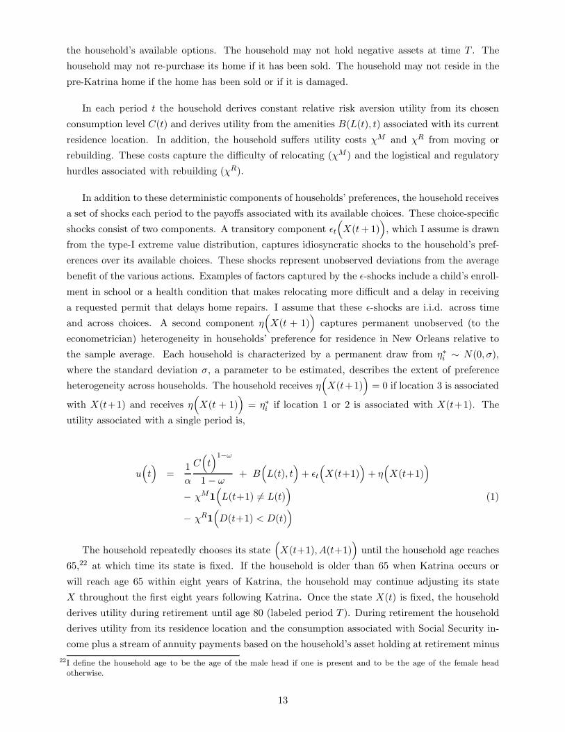
In each period t the household derives constant relative risk aversion utility from its chosen

consumption level C(t) and derives utility from the amenities B(L(t), t) associated with its current

residence location. In addition, the household suffers utility costs χM and χR from moving or

rebuilding. These costs capture the difficulty of relocating (χM ) and the logistical and regulatory

hurdles associated with rebuilding (χR).

In addition to these deterministic components of households’ preferences, the household receives

a set of shocks each period to the payoffs associated with its available choices. These choice-specific

shocks consist of two components. A transitory component εt

(X(t+ 1)

), which I assume is drawn

from the type-I extreme value distribution, captures idiosyncratic shocks to the household’s pref-

erences over its available choices. These shocks represent unobserved deviations from the average

benefit of the various actions. Examples of factors captured by the ε-shocks include a child’s enroll-

ment in school or a health condition that makes relocating more difficult and a delay in receiving

a requested permit that delays home repairs. I assume that these ε-shocks are i.i.d. across time

and across choices. A second component η(X(t + 1)

)captures permanent unobserved (to the

econometrician) heterogeneity in households’ preference for residence in New Orleans relative to

the sample average. Each household is characterized by a permanent draw from η∗i ∼ N(0, σ),

where the standard deviation σ, a parameter to be estimated, describes the extent of preference

heterogeneity across households. The household receives η(X(t+1)

)= 0 if location 3 is associated

with X(t+1) and receives η(X(t + 1)

)= η∗i if location 1 or 2 is associated with X(t+1). The

utility associated with a single period is,

u(t)

=1

α

C(t)1−ω

1 − ω+ B

(L(t), t

)+ εt

(X(t+1)

)+ η(X(t+1)

)

− χM1(L(t+1) 6= L(t)

)(1)

− χR1(D(t+1) < D(t)

)

The household repeatedly chooses its state(X(t+1), A(t+1)

)until the household age reaches

65,22 at which time its state is fixed. If the household is older than 65 when Katrina occurs or

will reach age 65 within eight years of Katrina, the household may continue adjusting its state

X throughout the first eight years following Katrina. Once the state X(t) is fixed, the household

derives utility during retirement until age 80 (labeled period T ). During retirement the household

derives utility from its residence location and the consumption associated with Social Security in-

come plus a stream of annuity payments based on the household’s asset holding at retirement minus

22I define the household age to be the age of the male head if one is present and to be the age of the female headotherwise.

13

any mortgage or rent payments associated with the chosen residential location. The household’s

objective is to maximize the present discounted value of future per-period utilities, denoted by U .

U =T∑

t=0

βt u(t)

(2)

where β is a subjective discount factor.

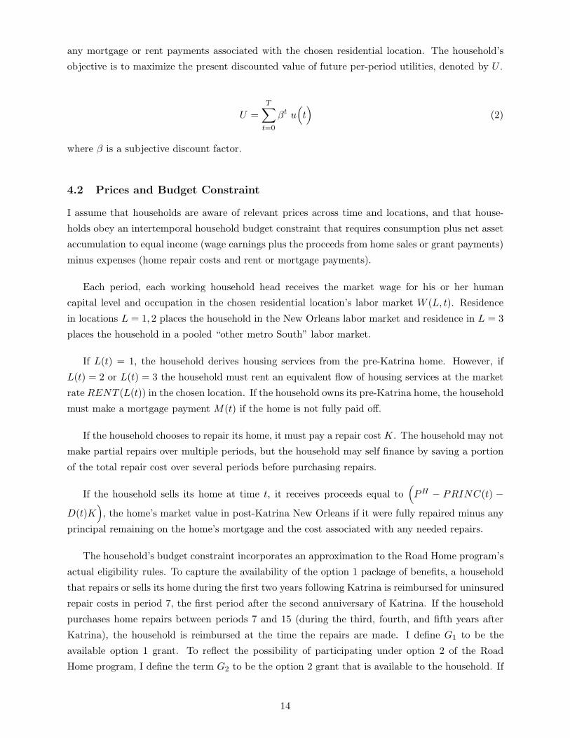
4.2 Prices and Budget Constraint

I assume that households are aware of relevant prices across time and locations, and that house-

holds obey an intertemporal household budget constraint that requires consumption plus net asset

accumulation to equal income (wage earnings plus the proceeds from home sales or grant payments)

minus expenses (home repair costs and rent or mortgage payments).

Each period, each working household head receives the market wage for his or her human

capital level and occupation in the chosen residential location’s labor market W (L, t). Residence

in locations L = 1, 2 places the household in the New Orleans labor market and residence in L = 3

places the household in a pooled “other metro South” labor market.

If L(t) = 1, the household derives housing services from the pre-Katrina home. However, if

L(t) = 2 or L(t) = 3 the household must rent an equivalent flow of housing services at the market

rate RENT (L(t)) in the chosen location. If the household owns its pre-Katrina home, the household

must make a mortgage payment M(t) if the home is not fully paid off.

If the household chooses to repair its home, it must pay a repair cost K. The household may not

make partial repairs over multiple periods, but the household may self finance by saving a portion

of the total repair cost over several periods before purchasing repairs.

If the household sells its home at time t, it receives proceeds equal to(PH − PRINC(t) −

D(t)K)

, the home’s market value in post-Katrina New Orleans if it were fully repaired minus any

principal remaining on the home’s mortgage and the cost associated with any needed repairs.

The household’s budget constraint incorporates an approximation to the Road Home program’s

actual eligibility rules. To capture the availability of the option 1 package of benefits, a household

that repairs or sells its home during the first two years following Katrina is reimbursed for uninsured

repair costs in period 7, the first period after the second anniversary of Katrina. If the household

purchases home repairs between periods 7 and 15 (during the third, fourth, and fifth years after

Katrina), the household is reimbursed at the time the repairs are made. I define G1 to be the

available option 1 grant. To reflect the possibility of participating under option 2 of the Road

Home program, I define the term G2 to be the option 2 grant that is available to the household. If

14

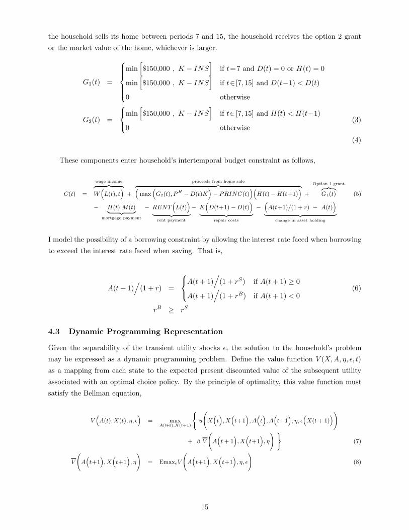
the household sells its home between periods 7 and 15, the household receives the option 2 grant

or the market value of the home, whichever is larger.

G1(t) =

min[$150,000 , K − INS

]if t=7 and D(t) = 0 or H(t) = 0

min[$150,000 , K − INS

]if t∈ [7, 15] and D(t−1) < D(t)

0 otherwise

G2(t) =

min

[$150,000 , K − INS

]if t∈ [7, 15] and H(t) < H(t−1)

0 otherwise(3)

(4)

These components enter household’s intertemporal budget constraint as follows,

C(t) =

wage income︷ ︸︸ ︷W(L(t), t

)+

proceeds from home sale︷ ︸︸ ︷(

max(G2(t), P

H − D(t)K)− PRINC(t)

)(H(t) − H(t+1)

)+

Option 1 grant︷ ︸︸ ︷G1(t) (5)

− H(t) M(t)︸ ︷︷ ︸

mortgage payment

− RENT(L(t)

)

︸ ︷︷ ︸rent payment

− K(D(t+1) − D(t)

)

︸ ︷︷ ︸repair costs

−(A(t+1)/(1 + r) − A(t)

)

︸ ︷︷ ︸change in asset holding

I model the possibility of a borrowing constraint by allowing the interest rate faced when borrowing

to exceed the interest rate faced when saving. That is,

A(t+ 1)/

(1 + r) =

A(t + 1)

/(1 + rS) if A(t + 1) ≥ 0

A(t + 1)/

(1 + rB) if A(t + 1) < 0(6)

rB ≥ rS

4.3 Dynamic Programming Representation

Given the separability of the transient utility shocks ε, the solution to the household’s problem

may be expressed as a dynamic programming problem. Define the value function V (X,A, η, ε, t)

as a mapping from each state to the expected present discounted value of the subsequent utility

associated with an optimal choice policy. By the principle of optimality, this value function must

satisfy the Bellman equation,

V(A(t),X(t), η, ε

)= max

A(t+1),X(t+1)

{

u

(

X(t), X(t+1

), A(t), A(t+1

), η, ε

(X(t + 1)

))

+ β V

(A(t + 1

), X(t+1

), η

) }(7)

V

(

A(t+1

), X(t+1

), η

)

= EmaxεV

(

A(t+1

), X(t+1

), η, ε

)

(8)

15

Because the choice specific ε shocks vary with X(t+1) but not A(t+1), the optimal asset accumulation

policy is a deterministic function of the current state and the chosen state, and Equation (7) may

be rewritten as,

V(A(t), X(t), η, ε

)= max

X(t+1)

{

u

(

X(t), X(t+1

), A(t), A∗

(X(t), η, X(t+1), A(t), t

), η, ε

(X(t + 1)

))

+ β V

(A∗

(X(t), η, X(t+1), A(t), t

), X(t+1

), η

) }(9)

where A∗(X(t), η,X(t+1), A(t), t

)is the optimal asset accumulation policy conditional on the

household’s initial state (X,A) and chosen state (X).

A∗

(X(t), η, X(t+1), A(t), t

)= arg max

A(t+1)

{

u

(

X(t), X(t+1

), A(t), A(t+1

), η, ε

(X(t + 1)

))

+ β V

(A(t + 1

), X(t+1

), η

) }(10)

This representation is convenient for estimation, because it allows for households’ financial assets

(which are not observed in the data) to be conditioned out of the likelihood function. In practice, I

discretize the asset space, so for any current state and chosen state the definition of A∗ in Equation

(10) requires finding the maximal element in a finite set.

The assumption that the ε shocks are drawn from the type I extreme value distribution allows for

a closed form representation of the expected maximal continuation value from any state (McFadden,

1975; Rust, 1987),

V(A(t), X(t), η

)= (11)

ln

∑

X(t+1)

exp(u(X(t), η, X(t+1), A(t),A∗

(X(t), η, X(t+1), A(t), t

))+ V

(A(t+1), X(t+1), η

))

+ γ

where γ ≈ 0.577 is Euler’s constant. Also, the conditional choice probabilities take the multinomial

logit form,

P(X(t+1)

∣∣∣A(t),X(t), η)

=

exp[u(X(t), η, X(t+1), A(t),A∗

(X(t), η, X(t+1), A(t), t

))+ V

(A(t+1), X(t+1), η

)]

∑X′(t+1) exp

[u(X(t), η, X ′(t+1), A(t),A∗

(X(t), η, X ′(t+1), A(t), t

))+ V

(A(t+1), X ′(t+1), η

)] (12)

Using these simplifications, it is straightforward to numerically solve the value function for any given

parameterization of the model using backward induction from the time T boundary condition.

16

5 Model Parameterization and Estimation

The parameters of the model to be estimated include a wage equation, a set of household preferences,

and the interest rate at which households may borrow. I estimate the model sequentially. The first

step estimates the wage equation. The second step takes the first step’s estimates as a known input

and estimates the parameters describing households’ preferences and the borrowing interest rate.

5.1 Wages

Each period, each household head who was employed during the year prior to Katrina receives a

wage that reflects the value of his or her skills in the worker’s residence location. That wage is

determined by,

lnwjklt = lnwklt + x′jβ + µj (13)

where j indexes workers, k indexes two-digit occupations, l indexes the labor market in which the

worker resides, t indexes the period, wklt is a period-location-specific mean occupation wage, xj is

a vector of worker human capital variables, and µj is a worker fixed effect.

I estimate this equation using pre-Katrina annual earnings records from DNORS23 and annual

earnings records from the New Orleans MSA respondents to the 2005 ACS. Pre-Katrina New

Orleans mean occupation wages wklt come from the 2005 ACS. I obtain estimates of the worker

fixed effects µj by computing the residuals from this regression for all DNORS records used to

estimate equation (13).

Estimation of the structural model requires an estimate of the labor wages that each household

faces in each location in each period. To construct these quantities, I compute the sum of the wages

predicted by equation (13) for each household’s working head or heads. I compute the location-

specific mean occupation wages that enter the right-hand side of equation (13) using the ACS. In

the model, each location’s mean occupation wages follow their observed paths in the ACS during

the first four years following Katrina and remain at their 2009 levels in each location in all later

years. Households with just one head who was employed during the year prior to Katrina receive

that worker’s wages, and couple-headed households with two working heads receive the sum of both

workers’ wages.

5.2 Parameterizing household’s preferences and the borrowing interest rate

Two parameters describe the consumption component of utility α

(C1−ω

1 − ω

), the coefficient of rel-

ative risk aversion ω and a parameter α that scales the importance of consumption utility relative

to that of the unobserved utility shocks ε.

23I estimate the wage equation using DNORS workers living in both renter-occupied and owner-occupied dwellings.

17

I normalize the borrowing interest rate for a group of relatively affluent households (non-black

households in which at least one household head holds a bachelor’s degree and pre-Katrina with

annual income exceeded $40k) to the risk-free rate (1/β). Affluent households were likely to be

eligible for the SBA Disaster Loan program or private loans. The borrowing interest rate for other

households differs from the risk-free rate according to,

ln(1 + rB) = ln(1/β) + γ11(black) + γ21(nocoll) + γ31(Inc < $20k) + γ41($20k < Inc < $40k)(14)

where 1(black) indicates that a household has a black household head, 1(nocoll) indicates that no

household head has a bachelor’s degree, and 1(Inc < $20k) and 1($20k < Inc < $40k) indicate

that pre-Katrina annual household income fell in the indicated range. A positive value for any of

the γ parameters indicates that on average the corresponding group faced borrowing constraints.

When estimating the location preference parameters, I normalize the payoff to living away from

New Orleans B(L = 3) to zero. The payoff B(L = 2) and the difference B(L = 1) − B(L = 2)

are parameters to be estimated. I allow these parameters to depend on a small set of household

and neighborhood characteristics. This parameterization captures differences in the benefits to

living in neighborhoods with different levels of flood damage and captures systematic differences in

attachment to place across groups.24

Following earlier structural migration studies (Kennan and Walker, 2011; Bishop, 2007), the

utility cost to moving χM depends on the distance and timing of the move.25 The utility cost to

repairing one’s home χR depends on whether the home was destroyed or the home was damaged

but not destroyed.

When discussing the estimation algorithm, I jointly refer to the set of model parameters de-

scribed here with θ = [B(L), χM , χR, rB, α, σ]′.

5.3 Estimation

When estimating the model, I follow earlier dynamic discrete choice studies of migration (Kennan

and Walker, 2011) by setting the subjective discount factor β = 0.95 annually. I set the coefficient

24Specifically, I allow B(L = 2) to follow a linear time trend during the first five years following Katrina. I allowB(L = 1, t) − B(L = 2, t) to depend on the fraction of owner-occupied homes on the same block segment (theDNORS sampling unit) that were rendered uninhabitable by Katrina. I group this continuous measure into threegroups; 0%− 50%, 50%− 90%, and 90%− 100%. I allow B(L = 1, t)−B(L = 2, t) to follow linear time trends duringthe first five years following Katrina within the two higher damage categories. This parameterization allows for thepossibility that living in a neighborhood that was heavily flooded might have been especially unappealing shortlyafter Katrina but may become more attractive as time passes. I also allow B(L = 1, t) − B(L = 2, t) to depend onthe 2000 poverty rate in the household’s Census block group, when the household purchased its home, and whethereither head was born outside of Louisiana.

25Specifically, the utility cost of moving depends on an indicator for any change in location, an indicator that the movewas to or from New Orleans (not within the city), and an indicator that the move occurred during the first periodafter a home repair. This parameterization allows for the possibilities that moving is more difficult if the destinationis far away, moving home is more likely immediately following a home repair, and the moving cost is different duringthe first period after Katrina than in subsequent periods.

18

of relative risk aversion ω = 4.17, the mean coefficient of relative risk aversion estimated by Barsky

et al. (1997) using an experimental approach with Health and Retirement Study data. As part

of a sensitivity analysis, I re-compute the model estimates and resulting policy simulations using

alternative values for ω.

To estimate the parameter-vector θ, assume that a sample of households i = 1, ..., N solve the

above model. For each household, I observe the sequence of choices{Xi(t)

}T

t=1. I do not observe

households’ initial financial asset holding, its permanent preference shock η, or its choice specific

utility shocks ε.

Conditional on an asset holding at time zero, the subsequent asset holding A∗ is a latent variable

whose path is determined within the model. This feature of the model allows for the likelihood of an

observed panel to be computed from observed choices if the initial asset holding is known. Because

the initial asset holding is unobserved, I condition that unobserved state out of the likelihood

function by computing each household’s observed choices at a range of initial asset values and

integrating those conditional likelihoods with respect to an auxiliary estimate of each household’s

distribution of initial asset holdings F iA0

(a) (described further below).

For a given value of Ai(0), I compute the model’s implied latent asset path consistent with a

household’s observed choice sequence using,

Ai

(t∣∣∣{Xi(τ)

}, A(0), η, θ

)=

Ai(0) if t = 0

A∗(Xi(t− 1),Xi(t), Ai(t− 1), t− 1

)if t > 0

(15)

where the function A∗() is defined in Equation (10). I use this asset path when computing the likeli-

hood function for a given household. Conditional on an assumed initial asset value, the household’s

likelihood contribution is:

li

(θ∣∣∣{Xi(t)

}T

t=1, A(0), η

)= Π11

t=0P(Xi(t+1)

∣∣∣Xi(t), Ai(t|A(0)), η, θ)

(16)

The household’s unconditional likelihood contribution may be obtained by integrating this condi-

tional expression with respect to the distribution of initial assets F iA(0)(a0) and the distribution of

the unobserved heterogeneity term Gη(η|θ):

li

(θ∣∣∣{Xi(t)

}T

t=1

)=

∫ ∫li

(θ∣∣∣{Xi(t)

}T

t=1, Ai(t|a0), η

)dF i

A(0)(a0) dGη(η|θ) (17)

Following Kennan (2004), I use discrete approximations to the continuous distribution F of

initial household asset holdings (10 support points) and the continuous distribution G of the het-

erogeneity term η (5 support points). To approximate the distribution of initial asset holdings,

19

I obtain an estimate of the 5th, 15th, ..., 95th percentiles of the distribution of each household’s

pre-Katrina asset holding conditional on the household’s observed characteristics. Appendix III

describes the approach in detail, which I apply to data from the 2005 wave of the PSID. Following

Kennan (2004), I approximate F iA0

(a) by imposing that the household’s prior probability of coming

from each of the 5th, 15th, ..., 95th percentiles of its initial asset-holding distribution is 1/10 and by

imposing that the household’s prior probability of coming each of 10th, 30th, 50th, 70th and 90th

percentiles of the distribution of η is 1/5. The integral in Equation 17 may then be approximated

by,

li(θ∣∣∣{

Xi(t)}T

t=1

)=

1

10

95∑

pa=5

1

5

90∑

pη=10

li(

θ∣∣∣{

Xi(t)}T

t=1, Ai(0)=F i−1

A(0)(pa), η=Gi−1η (pη)

)(18)

The log-likelihood for the full panel dataset is the log of the product of the individual household

likelihood contributions:

L(θ∣∣∣{X(t)}T

t=1

)= ln

(ΠN

i=1li

(θ∣∣∣{Xi(t)

}T

t=1

))(19)

Using this expression, I compute a nested fixed point estimator of θ. An “inner loop” computes a

numerical solution to the model and obtains a sample log-likelihood at a particular value of θ, and

an “outer loop” searches the parameter space for the likelihood maximizing parameter vector θ.

I conduct inference using the asymptotic variance-covariance matrix, robust to clustering at the

neighborhood level,26

COVθ

= H(θ)−1( K∑

k=1

gk(θ)gk(θ)′)H(θ)−1 (20)

where H(θ) = ∂2L(θ)/∂θ∂θ′ is the Hessian matrix and gk(θ) =∑

N (i)=k ∂li(θ)/∂θ is the sum of

household scores within cluster (neighborhood) k (N (i) returns household i’s neighborhood and j

indexes neighborhoods).

5.4 Identification

The assumption that the idiosyncratic component of the choice-specific preference shocks is drawn

from the Type-I EV distribution normalizes the variance of that unobserved component. Therefore,

as in a standard static logit model, the values of other parameters reflect their importance relative

to the importance of unobservables.

26I cluster by official New Orleans neighborhoods. That unit of geography is larger than Census blocks or block groups,so this approach is more conservative than clustering at these smaller units of geography at which some of the model’sexogenous variables are defined.

20

The importance of financial incentives to households’ location decisions is identified by varia-

tion in relative wages (wages in New Orleans minus wages in other Southern metro areas) across

occupations and time and variation in the financial incentive to rebuild provided by the provisions

of the Road Home grant program. The pre-Katrina occupations of households’ workers generate

variation in the time paths of their expected post-Katrina wages across locations. In New Orleans,

comparatively high wages were paid to occupations concentrated in industries that produced the

goods and services necessary for the region’s reconstruction. Comparatively low wages were paid to

occupations concentrated in industries that produce goods and services whose demand is especially

dependent on a sizeable permanent population. Second, the Road Home grant program paid more

generous net compensation to households that chose to rebuild (option 1) than those who chose

to relocate (options 2 and 3). The difference between the generosity of the various options varied

substantially across households depending on the extent of storm damage to the household’s home

and the fraction of the household’s repair costs that were covered by insurance payments.

The model’s effective borrowing rate parameters are identified in two ways. The first source

of identification resembles an approach developed by Cameron and Taber (2004) who, in the con-

text of higher education attainment, demonstrate that an effective borrowing rate is identified by

comparing how an investment choice (college attendance) varies with the direct cost of investing

and with a gradually accruing opportunity cost to investing. For an agent who is free to borrow,

the choice of whether to make a particular investment should be similarly influenced by a change

in the direct cost of the investment and an equivalent change in (the present value of) a gradually

accruing opportunity cost. On the other hand, for an agent who is borrowing constrained, the

choice should respond more strongly to a change in the direct cost of an investment, because for

a constrained agent the marginal utility of consumption will be highest in the period in which the

direct cost is paid. In the case of post-Katrina rebuilding, repair costs that are not covered by

insurance payments represent a direct cost that must be paid before returning to the pre-Katrina

residence. The difference between expected labor earnings in the evacuation location and New

Orleans represents a gradually accruing opportunity cost to returning and rebuilding.

A second source of identification involves examining the extent to which the propensity to

rebuild jumps at the time that Road Home grants are dispersed. This approach resembles an

approach found in the macroeconomics literature on consumption that tests the Permanent Income

Hypothesis by examining the consumption response to fully anticipated income windfalls (Shea,

1995; Souleles, 1999; Stephens, 2003). I impose that households in an affluent comparison group

(non-black households with a bachelor’s degree and with annual pre-Katrina income above $40,000

per year) may borrow at the risk free rate, since households in that group would have been very

likely to be eligible for government’s subsidized SBA disaster loan program. If, following the

payment of Road Home grants, the rebuilding rate of a particular group changes similarly to the

rebuilding rate of this (freely borrowing) comparison group, one could infer that the group also

faced low borrowing costs.

The flow benefit to the various residence locations is identified by the fraction of households

21

choosing each location after accounting for the financial incentives to do so. I normalize the flow

benefit to remaining away from New Orleans B(3) to zero. If the fraction of households that chose

to return to their pre-Katrina home exceeds the fraction predicted to do so based on financial

incentives alone then one may infer that the flow benefit to residence in the pre-Katrina home B(1)

is positive. The flow benefit to residing “elsewhere in New Orleans” B(2) is identified similarly. The

parameterization of the model allows B(1) to vary with neighborhood and household characteristics.

The parameters that describe how B(1) differs with particular pre-determined neighborhood and

household characteristics are identified by cross-sectional variation in those traits.

I allow for a utility cost to moving, following earlier dynamic discrete choice models of migration

(Kennan and Walker, 2011; Bishop, 2007). Because of its potentially important role in the post-

Katrina context, I also allow for a utility cost to repairing one’s home. To see the sort of variation

that allows for these sorts of “transition” costs (moving costs and repair costs both reduce the payoff

to particular state transitions) to be identified separately from the states’ flow benefits, consider

transitions involving two states, x1 and x2, which each provide a flow benefit. Optimality requires

that the state transition probabilities P (Xt+1 = x1|Xt = x1) and P (Xt+1 = x1|Xt = x2) both

increase with the flow benefit of state x1, but that the first quantity increases with the transition

cost and the second quantity decreases with the transition costs. With knowledge of the distribution

of unobservables, these two moments are sufficient to separately identify the transition cost and

the difference between the flow payoffs in x1 and x2.

Finally the scale of η, the persistent unobserved heterogeneity in the flow benefit that households

derive from residence in New Orleans, is identified from the degree of persistence in observed

choices. To see this, consider two extreme cases. If the scale of unobserved heterogeneity approaches

infinity, few households will be near the margin with respect to their residence location choices.

Households will quickly reveal their “types” by taking residence in New Orleans or away from New

Orleans, and initial location choices will be extremely persistent. In the other extreme, the i.i.d.

idiosyncratic preference shocks are the only unobserved influence on households’ choices. In that

case, choice probabilities depend only on a household’s current state, and otherwise do not vary

with the household’s state history. The estimator for the scale of persistent unobserved preference

heterogeneity is that which best rationalizes the persistence in observed choices, which presumably

falls between these two extremes.

6 Parameter Estimates and Model Fit

Table 4 presents estimates of the labor wage equation. In the second step of estimation, the labor

wages available to households across time and space are inferred from this equation and mean

year-location-occupation specific wages computed from the ACS. Figure 5 plots the time paths of

relative wages (log of mean New Orleans wages minus log of mean other Southern metro wages)

for several example occupations. In post-Katrina New Orleans, comparatively high wages prevailed

in occupations, like construction, concentrated in industries that produced the goods and services

22

necessary for the region’s reconstruction. Comparatively low wages prevailed in occupations, like

personal service providers and healthcare technicians, that are concentrated in industries that pro-

duce goods and services whose demand is especially dependent on a sizeable permanent population.

Table 5 provides estimates of the full model’s structural parameters. The estimates find that,

all else equal, households have a strong preference for living in New Orleans, and specifically in

their pre-Katrina homes. This estimate is driven by several features of the underlying data. By

Katrina’s fourth anniversary, majorities of households had returned to New Orleans, had maintained

ownership of their homes, and had repaired their homes. For most households those choices were

subsidized. But similar patterns occurred even among households with a negative financial return

to rebuilding — namely households with a small Road Home-induced incentive to rebuild and who

worked in occupations for which New Orleans offers comparatively low wages.

The flow benefits to residing on blocks with 50% − 90% or 90% − 100% of homes initially

uninhabitable follow statistically significantly positive time trends. Living in these areas was an

extremely undesirable option immediately following Katrina, but the benefit to residing in these

areas increased over time. The estimates find no statistically significant differences in flow location

benefits between block damage categories five years or more after Katrina.

My estimate of the borrowing rate equation finds that the effective borrowing rate is 41 log-

points higher than the saving interest rate for households with a pre-Katrina income less than $20k

per year, 35 log points higher for households with no bachelor’s degree, and 14 log-points higher

for black households. These estimates suggest that large segments of New Orleans households were

constrained in their rebuilding choices in Katrina’s immediate aftermath by low access to credit.

Consistent with other studies that estimate structural models of migration, I find that the

utility cost to moving is large relative to income. For instance, a median-income household would

be indifferent between paying the estimated baseline moving cost of 2.786 utils and suffering a

one-period consumption reduction of just above 90%. One might expect that returning to New

Orleans soon after Katrina would be especially difficult. The mandatory evacuation of the city

lasted for more than a month, and a lack of basic city services made returning difficult even after

some areas of the city were officially reopened. Indeed, I find that the moving cost is especially

high during the first period following Katrina. Finally, the moving cost is higher for moves to or

from New Orleans than for within-city moves.

The estimated utility cost to repairing a home is on the same order as the utility cost to moving.

As expected, the utility cost to repairing a destroyed home is significantly higher than the utility

cost of repairing an a home that was uninhabitable but not destroyed following Katrina.

The estimated standard deviation of η, the term capturing persistent unobserved heterogeneity

in the preference for living in New Orleans, is 0.65 utils. This parameter is difficult to interpret

23

directly, so it is useful to consider the location preferences of households with η draws one stan-

dard deviation above average and one standard deviation below average. A household with η= 0

belonging to the reference category of the location flow-benefit equations receives a long-term flow

benefit to residing in the pre-Katrina home of about 0.5 utils per period. A household with η

one standard deviation below average has a slight preference for living away from New Orleans,

all else equal, since 0.5+(−0.65)< 0. A household with η one standard deviation above average

has an extremely strong preference for living in the pre-Katrina home relative to living away from

New Orleans, about 0.5+0.65 = 1.1 utils per period. Holding other location costs and amenities

constant, a median income household with these location preference would be willing to remain in

the pre-Katrina home and accept a reduction in non-housing consumption of over 95% instead of

relocating away from New Orleans.

Table 6 assesses the model’s fit. I compare the model’s predicted fraction of households exhibit-

ing four different outcomes to the empirical fraction of households exhibiting those outcome on the

first four anniversaries of Katrina. I provide similar comparisons within the sample of households

with initially uninhabitable homes and within three sub-samples defined by pre-Katrina household

income. For each comparison, I report a cluster-corrected (clustered at the neighborhood level)

chi-squared test statistic associated with the null that the predicted moment and the sample mo-

ment are equal. The model predicts the key features of the data quite well, but the model’s fit is

not exact in a number of places. Among the four outcomes considered, the fraction of households

having sold their homes is matched least closely, and the formal chi-squared tests reject the model’s

fit to that outcome in several instances.

7 Policy Simulations

The remainder of this paper describes the results of simulation experiments designed to examine

how several aspects of disaster-relief policy influence households’ behavior.

I conduct simulations of households’ choices under a baseline scenario, in which households

face the actual post-Katrina policy environment, and under several alternative scenarios in which

particular policies are changed one at a time. For each scenario, I compute 10,000 simulated panels

for each household, initializing each panel using the household’s actual location L and home damage

status D in the first period after Katrina. I compute 1/50th of each household’s simulated panels

at each of the 50 combinations of the A(0) and η used to approximate the distributions of those

quantities during estimation. When computing mean outcomes from the simulated data, I weight

each simulated panel by the ex post probability that a household falls at the particular A(0) × η

combination conditional on the household’s actual choice sequence.27

27The ex post probability that a household is characterized by a given combination of an initial asset holding and η-draw

is equal to 0.02 × l(θ∣∣∣{

Xi(t)}T

t=1, A(0), η

)/l(θ∣∣∣{

Xi(t)}T

t=1

), that is, the ex-ante weight (1/50) times the ratio of

the household’s panel’s likelihood conditional on an A(0) × η combination to the household’s panel’s unconditionallikelihood.

24

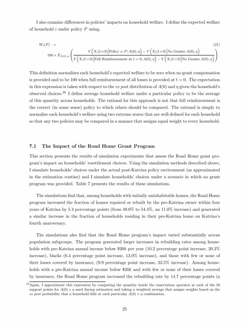
I also examine differences in policies’ impacts on household welfare. I define the expected welfare

of household i under policy P using,

Wi(P ) = (21)

100 × EA(0),η

V(Xi(t=0)

∣∣∣Policy = P ;A(0), η)− V

(Xi(t=0)

∣∣∣No Grants; A(0), η)

V(Xi(t=0)

∣∣∣Full Reimbursement at t = 0; A(0), η)− V

(Xi(t=0)

∣∣∣No Grants; A(0), η)

This definition normalizes each household’s expected welfare to be zero when no grant compensation

is provided and to be 100 when full reimbursement of all losses is provided at t = 0. The expectation

in this expression is taken with respect to the ex post distribution of A(0) and η given the household’s

observed choices.28 I define average household welfare under a particular policy to be the average

of this quantity across households. The rational for this approach is not that full reimbursement is

the correct (in some sense) policy to which others should be compared. The rational is simply to

normalize each household’s welfare using two extreme states that are well-defined for each household

so that any two policies may be compared in a manner that assigns equal weight to every household.

7.1 The Impact of the Road Home Grant Program

This section presents the results of simulation experiments that assess the Road Home grant pro-

gram’s impact on households’ resettlement choices. Using the simulation methods described above,

I simulate households’ choices under the actual post-Katrina policy environment (as approximated

in the estimation routine) and I simulate households’ choices under a scenario in which no grant

program was provided. Table 7 presents the results of these simulations.

The simulations find that, among households with initially uninhabitable homes, the Road Home

program increased the fraction of homes repaired or rebuilt by the pre-Katrina owner within four

years of Katrina by 5.4 percentage points (from 49.0% to 54.4%, an 11.0% increase) and generated

a similar increase in the fraction of households residing in their pre-Katrina home on Katrina’s

fourth anniversary.

The simulations also find that the Road Home program’s impact varied substantially across

population subgroups. The program generated larger increases in rebuilding rates among house-

holds with pre-Katrina annual income below $20k per year (10.2 percentage point increase, 20.2%

increase), blacks (6.4 percentage point increase, 13.0% increase), and those with few or none of

their losses covered by insurance, (9.9 percentage point increase, 22.5% increase). Among house-

holds with a pre-Katrina annual income below $20k and with few or none of their losses covered

by insurance, the Road Home program increased the rebuilding rate by 14.7 percentage points (a

28Again, I approximate this expression by computing the quantity inside the expectation operator at each of the 50support points for A(0)× η used during estimation and taking a weighted average that assigns weights based on theex post probability that a household falls at each particular A(0) × η combination.

25

34.0% increase). The program generated smaller impacts on rebuilding rates among non-blacks

(3.2 percentage point increase, 6.7% increase) and those with all or most of their losses covered by

insurance (0.7 percentage point increase, 1.2% increase).

Table 8 compares the Road Home program’s impact on households’ resettlement choices and

on households’ welfare to the impacts of counterfactual disaster relief policies. These comparisons

provide a better understanding of the mechanisms through which the Road Home program impacted

households’ welfare and choices. For each comparison, the first pair of columns report the results

using the full sample of households whose homes were initially uninhabitable following Katrina.

The second and third column pairs report the results for sub-samples of low-income households

(pre-Katrina annual income < $20k) and higher-income households (pre-Katrina annual income

> $40k).

The first three-row group in Table 8 compares the impact of the Road Home program to the

impact of a program that makes subsidized loans available to all households on Katrina’s second

anniversary (to approximately match the timing of the Road Home program’s “treatment”). These

simulations find that the expanded loan program generates an impact on the rate of residence in

the pre-Katrina home that is about 70% the size of the Road Home program’s impact, suggesting

that a large portion of Road Home’s treatment effect can be attributed to the program’s allowing

households that preferred to rebuild to overcome the initial hurdle of securing financing. Among

households with pre-Katrina annual income below $20k, the loan program’s impact is 87% the

size of Road Home’s impact, and among households with pre-Katrina annual income above $40k

the loan program’s impact is 55% the size of Road Home’s impact. Similarly, the loan program’s

impact on household welfare is 40% of Road Home’s impact on average, but is 69% of Road Home’s

impact among low-income households and just 25% of Road Homes impact among higher-income

households.

The second three-row group in Table 8 compares the Road Home program’s impact to the impact

of a program that pays option 1 grants to all households regardless of the resettlement choice. These

simulations find that a program that provides an option 1 grant to all households regardless of the

households’ resettlement choice generates about 97.5% of the Road Home program’s impact on

the fraction of households living in the pre-Katrina home. This finding suggests that the financial

incentive to rebuild generated by the difference in generosity between the Road Home program’s

option 1 grant and option 2 grant accounts for only a small fraction of the program’s impact on

household behavior.

I also report average household welfare under the policy that provides an option 1 to all house-

holds regardless of the households’ resettlement choices. This unconditional grant program’s impact

on average household welfare is about 75% higher than the impact of the actual Road Home pro-

gram. This calculation does not hold the program’s cost constant, and therefore does not necessarily

suggest that the Road Home program is sub-optimal within a class of equally expensive grant pro-

grams. Instead, these results simply suggest that, given the substantial heterogeneity in households’

26

preferences for living in New Orleans, two policies can have similar impacts on households’ location

choices even if the policies provide a dramatically different financial incentive for living in New

Orleans and have dramatically different effects on the welfare of inframarginal households.

The third three-row group compares the Road Home program’s impact to the impact of a

program with the same rules as the Road Home program but that paid grants at t = 0. The

simulations find that the fraction of households having rebuilt by Katrina’s fourth anniversary is

very similar under the actual Road Home program, which paid grants roughly two years after

Katrina, and under a grant program that paid grants immediately after Katrina. However, the

welfare effects of grant payments do depend on the timing of grant payments. The average welfare

effect of the immediately rolled out program is roughly one third larger than the welfare effect of the

actual Road Home program. This is because the immediately rolled out program allows households

with a strong preference for living in New Orleans to do so earlier. The difference between the

welfare effects of the immediately rolled out program and the later rolled out program was larger

among low-income households, because that group’s limited ability of to borrow makes the timing

of its rebuilding decisions especially sensitive to the timing of grant payments.

7.2 The Marginal Impact of Wage Subsidies and Direct grants

The Gulf Opportunity Zone program provided $2, 400-per-worker wage subsidies to employers who

hired or retained a worker who lived on the Gulf Coast just prior to Hurricane Katrina. In this

section I present the results of simulations that compare the marginal effect of $2, 400 per worker

boost in the present value of New Orleans labor wages (spread evenly over the first four years

following Katrina) to the impact of a $2, 400 per worker increase in the generosity of the Road

Home program’s option 1 grant. This comparison examines how the timing of a location subsidy

to a borrowing constrained population influences the effect of the subsidy on households’ location

choices. I include only working households in this comparison.

Table 9 presents the results of these simulation experiments. Both policy changes cause small

changes in behavior. However, the impact of the wage subsidy is only about half of the impact of an

equivalent change in the rebuilding grant. The effects of grants and wage subsidies differ because,

for borrowing constrained households, the benefit of a direct grant falls entirely in the period in

which repairs are purchased, when the marginal utility of consumption is high. Among households

with a pre-Katrina annual income less than $20k, the wage subsidy generates an impact that is only

about 20 of the impact generated by an equivalent change in the rebuilding grant. On the other

hand, among households with a pre-Katrina annual income above $40k, the wage subsidy generates

an impact that is about 70% of the impact generated by an equivalent change in the rebuilding

grant. These findings suggest that in the presence of borrowing constraints, wage subsidies are likely

to have a smaller impact on households’ resettlement choices than similarly sized direct grants. To

the extent that borrowing constraints are concentrated in segments of the population that have few

resources available for rebuilding, wage subsidies might even exacerbate disparities in rebuilding

rates across groups.

27

One should not conclude from these results alone that subsidies to local firms are an ineffective

means of providing disaster relief. To the extent that the incidence of these subsidies falls partially

to firms, the subsidies may increase the number of firms finding it (weakly) profitable to operate

in a disaster-affected area. Such a change may directly increase the flow benefit that a household

derives from living in the area, if the presence of more firms increases the ability of households to

obtain desired goods and services.

7.3 The Deadweight Loss from Disaster-Related Subsidies

Disaster-related location subsidies include up front subsidies like discounts to National Flood In-

surance Program premiums and guarantees of future payments in the event of a disaster. Both

types of subsidy reduce the expected cost of residing in a dangerous location. The size of the eco-

nomic distortion generated by these subsidies depends on the extent to which the subsidies induce

marginal households to alter their location decisions. As a final application of the model, I use the

model’s implied semi-elasticity of residence location with respect to housing costs to compute the

deadweight loss associated with a hypothetical subsidy for living in New Orleans.

I consider the effect of a flow subsidy for living in New Orleans measured as a fraction τ of

each household’s home’s value. For example, if τ = 1% then a household with a $100k home would

receive $1,000 per year. If the probability of a household’s home being destroyed by a disaster

is τ% each year, then this subsidy provides the actuarially fair value of an insurance policy that

guarantees full compensation when a disaster occurs. Therefore, I interpret the distortionary effects

of this policy as an approximation of the distortionary effects of a policy that guarantees relief in

the event of a disaster.

Let S(W − UCH) represent the long-run supply of households to New Orleans as a function of

the real wage, annual labor earnings minus the user cost of housing. In the presence of moving costs

and heterogeneity in location preferences across households, this supply curve slopes upward.29 The

subsidy generates a rightward shift in the supply curve, and therefore, if the labor demand and

housing supply have positive price elasticities, the subsidy increases the equilibrium population of

the city. To determine an upper bound on the deadweight loss of this subsidy, I consider the case

in which the long run price elasticities of labor demand and housing supply are both infinite. With

infinitely elastic labor demand and housing supply, none of the subsidy’s incidence falls to firms

or land developers (which would dampen the subsidy’s distortion of households’ location choices),

and the elasticity of supply of residents to the city is a sufficient statistic for the deadweight loss

associated with the subsidy.

29The classic Rosen-Roback model of spatial equilibrium (Rosen, 1979; Roback, 1982) and some applications of thatmodel in the modern local public finance literature (Albouy, 2009, for example) assume that moving is costlessand that preferences are homogeneous. That assumption immediate implies that in equilibrium, all individualsare indifferent between living in any location with population greater than zero and that the supply of residentsto locations is infinitely elastic with respect to the real local wage. In such a model, spatially targeted subsidiesmust generate large distortions. See Busso, Gregory, and Kline (2011) for an expanded discussion of the efficiencyconsequences of local subsidies in the presence of location-preference heterogeneity.

28

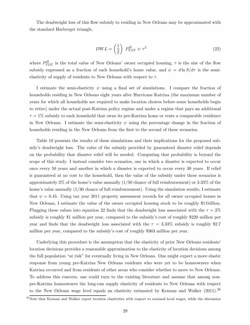
The deadweight loss of this flow subsidy to residing in New Orleans may be approximated with

the standard Harberger triangle,

DWL =

(1

2

)PH

TOT ψ τ2 (22)

where PHTOT is the total value of New Orleans’ owner occupied housing, τ is the size of the flow

subsidy expressed as a fraction of each household’s home value, and ψ = d lnS/dτ is the semi-

elasticity of supply of residents to New Orleans with respect to τ .

I estimate the semi-elasticity ψ using a final set of simulations. I compare the fraction of

households residing in New Orleans eight years after Hurricane Katrina (the maximum number of

years for which all households are required to make location choices before some households begin

to retire) under the actual post-Katrina policy regime and under a regime that pays an additional

τ = 1% subsidy to each household that owns its pre-Katrina home or rents a comparable residence

in New Orleans. I estimate the semi-elasticity ψ using the percentage change in the fraction of

households residing in the New Orleans from the first to the second of these scenarios.

Table 10 presents the results of these simulations and their implications for the proposed sub-

sidy’s deadweight loss. The value of the subsidy provided by guaranteed disaster relief depends

on the probability that disaster relief will be needed. Computing that probability is beyond the

scope of this study. I instead consider two scenarios, one in which a disaster is expected to occur

once every 50 years and another in which a disaster is expected to occur every 30 years. If relief

is guaranteed at no cost to the household, then the value of the subsidy under these scenarios is

approximately 2% of the home’s value annually (1/50 chance of full reimbursement) or 3.33% of the

home’s value annually (1/30 chance of full reimbursement). Using the simulation results, I estimate

that ψ = 0.45. Using tax year 2011 property assessment records for all owner occupied homes in

New Orleans, I estimate the value of the owner occupied housing stock to be roughly $11billion.

Plugging these values into equation 22 finds that the deadweight loss associated with the τ = 2%

subsidy is roughly $1 million per year, compared to the subsidy’s cost of roughly $220 million per

year and finds that the deadweight loss associated with the τ = 3.33% subsidy is roughly $2.7

million per year, compared to the subsidy’s cost of roughly $363 million per year.

Underlying this procedure is the assumption that the elasticity of prior New Orleans residents’

location decisions provides a reasonable approximation to the elasticity of location decisions among

the full population “at risk” for eventually living in New Orleans. One might expect a more elastic

response from young pre-Katrina New Orleans residents who were yet to be homeowners when

Katrina occurred and from residents of other areas who consider whether to move to New Orleans.

To address this concern, one could turn to the existing literature and assume that among non-

pre-Katrina homeowners the long-run supply elasticity of residents to New Orleans with respect

to the New Orleans wage level equals an elasticity estimated by Kennan and Walker (2011).30

30Note that Kennan and Walker report location elasticities with respect to nominal local wages, while the discussion

29

Kennan and Walker (2011) present estimates of the supply elasticity of residents to many locations

by simulating the effects of permanent changes to locations wages beginning when workers are 20,

and each estimate falls between 0.5 and 0.75. As another option for addressing this concern, one

might assume that among non-pre-Katrina homeowners the long-run supply elasticity of residents

to New Orleans with respect to the New Orleans wage level is well-approximated by the model’s

implied elasticity for young households. Figure 6 plots the model’s implied long-run elasticity

of New Orleans’ population with respect to the local wage separately for households of different

ages and finds that the elasticity for households under 35 is 0.96, compared to 0.22 among all

households.31 Columns 3 through 6 of Table 10 report additional estimates of the deadweight loss

from the hypothetical subsidies under additional scenarios that use the model’s implied elasticity of

location choices for households under 35 to approximate the long-run supply elasticity of residents

to New Orleans with respect to the New Orleans wage level. I choose the larger of the two available

elasticity estimates for that group so that the results are more likely to represent an upper bound

for the actual deadweight loss.

Columns 3 and 4 of Table 10 present calculations of the deadweight losses associated with the

same subsidies assuming a baseline under which 3/4 of households that reside in New Orleans

exhibit the model’s implied average location elasticity and 1/4 exhibit the higher location elasticity

found for young households. This 3 : 1 ratio is roughly the ratio found in New Orleans prior

to Katrina of Louisiana-native households to households with at least one head born outside of

Louisiana. In this scenario, the deadweight loss associated with a guarantee of relief in the event

of a future disaster is slightly less than 1% of the policy’s expected flow costs if a disaster occurs

with a probability of 1/50 each year, and the deadweight loss associated with a guarantee of relief

in the event of a future disaster is slightly more than 1% of the policy’s expected flow costs if a

disaster occurs with a probability of 1/30 each year. Finally, columns 5 and 6 of Table 10 compute

these deadweight losses under the assumption that all households exhibit the location elasticity

found for young households. This scenario is perhaps appropriate when considering the policies’

distortion over a very long horizon, perhaps multiple generations. However, even in this scenario

that assumes the most elastic response, the deadweight loss associated with the flow subsidy to

New Orleans is less than 3% of the policy’s expected cost.

Substantial heterogeneity in location preferences accounts for the relatively small size of these

deadweight loss figures relative to the subsidies’ expected flow costs. While disaster-related location

subsidies may comprise large difficult-to-justify transfers from residents of safe areas to residents

of dangerous areas, the distortions associated with these transfers appear to be relatively small.

in the previous paragraph considers location elasticities with respect to housing costs.31Again, household age is defined to be the age of the male household head if one is present and the age of the female

head otherwise.

30

8 Conclusion

This paper develops and estimates a dynamic structural model of pre-Katrina New Orleans home-

owners’ post-Katrina resettlement choices and uses the model to investigate the immediate and

long-term impacts of government disaster-relief policy. During the first two years following Hur-

ricane Katrina, low-income households and black households rebuilt damaged homes at a much

lower rate than higher-income households and non-black households. By the fourth anniversary of

Katrina, disparities in rebuilding rates had closed substantially. The structural model finds that

these patterns are best rationalized by a model in which pre-Katrina homeowners have a strong

preference on average for residing in New Orleans, there is substantial heterogeneity in the strength

of that location preference, and several large population subgroups face borrowing constraints.

Using the estimated model, I conduct a series of simulation experiments to assess the impact

of the Road Home rebuilding grant program on households’ resettlement choices and to assess the

relative impacts of wage subsidies and rebuilding grants. The simulation experiments find that the

Road Home program increased the fraction of households with severely damaged homes that had

rebuilt within four years by about 11%. The program’s impact occurred primarily within groups

that otherwise lacked the savings or ability to borrow that would have been necessary to finance

repairs or rebuilding if no grant program had been provided. A second set of simulation experiments

comparing the impact of direct grants to the impact of wage subsidies finds that, on the margin,

direct grants influence rebuilding rates by about twice the amount of similarly sized (in present

value terms) wage subsidies.

I then use the model’s implied elasticity of location choices with respect to financial incentives,

in the context of a simple general equilibrium framework, to assess the deadweight loss associated

with disaster-related location subsidies. The model finds that a guarantee of full compensation in

the event of a future disaster generates a deadweight loss that is about 1% of the subsidy’s expected

cost under the conservative assumption that a devastating disaster will occur on average once per

thirty years. While one may question the fairness of providing large transfers from safe locations

to unsafe locations, these results suggest that the distortionary effects of disaster-related location

subsidies are relatively small.

This paper considers a partial equilibrium model of households’ resettlement choices, and as

a consequence the policy experiments do not capture any general equilibrium price effects that

the programs might have had, and perhaps more importantly, do not capture any social spill-over

effects. A social spill-over would occur if, for instance, other things equal residing on a block on

which 50% of one’s neighbors had returned provided greater utility than residing on utility than

residing on a block on which 40% of one’s neighbors had returned. Capturing these types of effects

in a dynamic model presents considerable challenges for estimation, but would lead to a more

complete assessment of program impacts and will be one focus of my future work.

31

References

1. Aguirregabiria, V. and P. Mira (2010). “Dynamic discrete choice structural models: A survey.” Journal

of Econometrics 156(1): 38-67.

2. Arcidiacono, P. and J. B. Jones (2003). “Finite Mixture Distributions, Sequential Likelihood and the

EM Algorithm.” Econometrica 71(3): 933-946.

3. Albouy, D. (2009). “The Unequal Geographic Burden of Federal Taxation.” Journal of Political

Economy 117(4): 635-667.

4. Barsky, R., F. Juster, M. Kimball, and M. Shapiro (1997). “Preference Parameters and Behavioral

Heterogeneity: An Experimental Approach in the Health and Retirement Study.” The Quarterly

Journal of Economics 112(2): 537-579.

5. Bartik, T. J. (1991). “Who Benefits from State and Local Economic Development Policies?,” W.E.

Upjohn Institute for Employment Research.

6. Bishop, K. (2007). “A Dynamic Model of Location Choice and Hedonic Valuation.” Job Market

Paper.

7. Blanchard, O. J. and L. F. Katz (1992). “Regional Evolutions.”

8. Boarnet, M. G. and W. T. Bogart (1996). “Enterprise Zones and Employment: Evidence from New

Jersey.” Journal of Urban Economics 40(2): 198-215.

9. Bondonio, D. and J. Engberg (2000). “Enterprise zones and local employment: evidence from the

states’ programs.” Regional Science and Urban Economics 30(5): 519-549.

10. Bound, John and Harry J. Holzer (2000). “Demand Shifts, Population Adjustments, and Labor Market

Outcomes during the 1980s.” Journal of Labor Economics 18(1): 20-54

11. Busso, M, J. Gregory, P. Kline (2011). “Assessing the Incidence and Efficiency of a Prominent Place-

Based Policy.” Working Paper

12. Cameron, S. and C. Taber (2000). “Borrowing Constraints and the Returns to Schooling.” NBER

Working.

13. Cameron, S. V. and J. J. Heckman (2001). “The Dynamics of Educational Attainment for Black,

Hispanic, and White Males.” Journal of Political Economy 109(3): 455-499.

14. Chan, S. (2001). “Spatial Lock-in: Do Falling House Prices Constrain Residential Mobility?” Journal

of Urban Economics 49(3): 567-586.

15. de Leeuw, F. and N. F. Ekanem (1971). “The Supply of Rental Housing.” American Economic Review

61(5): 806-17.

16. Deaton, A. (1991). “Saving and Liquidity Constraints.” Econometrica 59(5): 1221-1248.

17. Elliott, J. R. and J. Pais (2006). “Race, class, and Hurricane Katrina: Social differences in human

responses to disaster.” Social Science Research 35(2): 295-321.

18. Elvery, J. A. (2009). “The Impact of Enterprise Zones on Resident Employment.” Economic Devel-

opment Quarterly 23(1): 44-59.

19. Engelhardt, G. V. (1996). “House prices and home owner saving behavior.” Regional Science and

Urban Economics 26(3-4): 313-336.

20. Evans, D. S. and B. Jovanovic (1989). “An Estimated Model of Entrepreneurial Choice under Liquidity

Constraints.” Journal of Political Economy 97(4): 808.

32

21. Federal Emergency Management Agency and Federal Insurance and Mitigation Administration. (2002).

“The National Flood Insurance Program: Program Description.” Government Report

22. French, E. and J. John Bailey (2011). “The Effects of Health Insurance and Self-Insurance on Retire-

ment Behavior.” Econometrica 79(3): 693732.

23. Fussell, E., N. Sastry, et al. “Race, socioeconomic status, and return migration to New Orleans after

Hurricane Katrina.” Population & Environment 31(1): 20-42.

24. Gallin, J. H. (2004). “Net Migration and State Labor Market Dynamics.” Journal of Labor Economics

22(1): 1-22.

25. Gemici, A. (2007). “Famiily Migration and Labor Market Outcomes.” Phd Dissertation.

26. Glaeser, E. L. and J. D. Gottlieb (2008). “The Economics of Place-Making Policies, National Bureau

of Economic Research, Inc.”

27. Glaeser, E.L. and J. Gyourko (2004) “Urban Decline and Durable Housing.” Journal of Political

Economy 113: 345-375.

28. Greenwood, M. J. (1985). “Human Migration: Theory, Models, and Empirical Studies.” Journal of

Regional Science 25(4): 521-544.

29. Groen, J. A. and A. E. Polivka (2009). “Going Home after Hurricane Katrina: Determinants of Return

Migration and Changes in Affected Areas.” Demography 47(4): 821-844.

30. Grummer-Strawn, L. M. (2003). “Regression Analysis of Current-Status Data: An Application to

Breast-Feeding.” Journal of the American Statistical Association 88(423): 758-765.

31. Harberger, Arnold. 1964. The Measurement of Waste. American Economic Review 54(3): 58-76.

32. Haurin, D. R., P. H. Hendershott, et al. (1996). “Borrowing Constraints and the Tenure Choice of

Young Households,” National Bureau of Economic Research, Inc.

33. Hotz, V. J., R. A. Miller, et al. (1994). “A Simulation Estimator for Dynamic Models of Discrete

Choice.” The Review of Economic Studies 61(2): 265-289.

34. Hubbard, R. G. and K. L. Judd (1987). “Social Security and Individual Welfare: Precautionary Saving,

Borrowing Constraints, and the Payroll Tax.” The American Economic Review 77(4): 630-646.

35. Ioannides, Y. M. and K. Kan (1996). “Structural Estimation of Residential Mobility and Housing

Tenure Choice.” Journal of Regional Science 36(3): 335-363.

36. Kamel, N. K. and A. Loukaitou-Sideris (2004). “Residential Assistance and Recovery Following the

Northridge Earthquake.” Urban Studies 41(3): 533-562.

37. Kates, R. W., C. E. Colten, et al. (2006). “Reconstruction of New Orleans after Hurricane Katrina:

A research perspective.” Proceedings of the National Academy of Sciences 103(40): 14653-14660.

38. Keane, M. P. and K. I. Wolpin (1994). “The Solution and Estimation of Discrete Choice Dynamic

Programming Models by Simulation and Interpolation: Monte Carlo Evidence.” The Review of Eco-

nomics and Statistics 76(4): 648-672.

39. Keane, M. P. and K. I. Wolpin (1997). “The Career Decisions of Young Men.” Journal of Political

Economy 105(3): 473-522.

40. Keane, M. P. and K. I. Wolpin (2001). “The Effect of Parental Transfers and Borrowing Constraints

on Educational Attainment.” International Economic Review 42(4): 1051-1103.

41. Keane, M. P. and K. I. Wolpin (2002). “Estimating Welfare Effects Consistent with Forward-Looking

Behavior. Part I: Lessons from a Simulation Exercise.” The Journal of Human Resources 37(3):

570-599.

33

42. Keane, M. P. and K. I. Wolpin (2002). “Estimating Welfare Effects Consistent with Forward-Looking

Behavior. Part II: Empirical Results.” The Journal of Human Resources 37(3): 600-622.

43. Kennan, J. (2004). “A Note on Approximating Distribution Functions.” Unpublished mimeo.

44. Kennan, J. and J. R. Walker (2011). “The Effect of Expected Income on Individual Migration Deci-

sions.” Econometrica 79(1): 211-251.

45. Linneman, P. and S. Wachter (1989). “The Impacts of Borrowing Constraints on Homeownership.”

Real Estate Economics 17(4): 389-402.

46. McCarthy, Kevin ; Peterson, D. J. ; Sastry, Narayan ; Pollard, Michael (2006). “The Repopulation of

New Orleans After Hurricane Katrina.” Technical report. RAND Corp.

47. Moretti, E. (2011). “Local Labor Markets.” Hanbook of Labor Economics.

48. Nichols, A. L. and R. Zeckhauser (1982). “Targeting Transfers through Restrictions on Recipients.”

American Economic Review 72(2): 372-77.

49. Ortalo-Magne, F. and S. Rady (2006). “Housing Market Dynamics: On the Contribution of Income

Shocks and Credit Constraints.” Review of Economic Studies 73(2): 459-485.

50. Papke, L. E. (1993). “What Do We Know about Enterprize Zones?,” National Bureau of Economic

Research, Inc.

51. Papke, L. E. (1994). “Tax policy and urban development : Evidence from the Indiana enterprise zone

program.” Journal of Public Economics 54(1): 37-49.

52. Paxson, C. and C. Rouse (2008). “Returning to New Orleans after Hurricane Katrina.” American

Economic Review 98(2): 38-42.

53. RAND Corporation (2010). “Restricted Data Files.” The Displaced New Orleans Residents Survey.

Website: http://www.rand.org/labor/projects/dnors.html

54. The Road Home Program (2006). “Checklist of Items to Bring to Your Initial Appointment.” Available

at URL: http://www.road2la.org/Docs/first_appt_items.pdf

55. Roback, J. (1982). “Wages, Rents, and the Quality of Life.” The Journal of Political Economy 90(6):

1257-1278.

56. Rosen, S. (1979). “Wage-Based Indixes of Urban Quality of Life.” Current Issues in Urban Economics.

57. Rosenzweig, M. and K. Wolpin (1993). “Credit Market Constraints, Consumption Smoothing, and

the Accumulation of Durable Production Assets in Low-Income Countries: Investment in Bullocks in

India.” Journal of Political Economy 101(2): 223-44.

58. Ruggles, S., J. T. Alexander, K. Genadek, R. Goeken, M. B. Schroeder, and M. Sobek. Integrated

Public Use Microdata Series: Version 5.0 [Machine-readable database]. Minneapolis: University of

Minnesota, 2010.

59. Rust, J. (1987). “Optimal Replacement of GMC Bus Engines: An Empirical Model of Harold Zurcher.”

Econometrica 55(5): 999-1033.

60. Rust, J. and C. Phelan (1997). “How Social Security and Medicare Affect Retirement Behavior In a

World of Incomplete Markets.” Econometrica 65(4): 781-831.

61. Shea, J. (1995). “Union Contracts and the Life-Cycle/Permanent-Income Hypothesis.” The American

Economic Review 85(1): 186-200

62. Shea, J. (2000). “Does parents’ money matter?” Journal of Public Economics 77(2): 155-184.

34

63. Sjaastad, L. A. (1962). “The Costs and Returns of Human Migration.” Journal of Political Economy

70(s5): 80.

64. Smith, S. and C. McCarty (1996). “Demographic Effects of Natural Disasters: a Case Study of

Hurricane Andrew.” Demography 33(2): 265-275.

65. Souleles, N. (1999). “The Response of Household Consumption to Income Tax Refunds.” The Amer-

ican Economic Review 89(4): 947-958.

66. State of Louisiana, Office of Community Development (2008). “The Road Home Homeowner Program

Policies Version 6.2.” Available at URL: https://www.road2la.org/Docs/policies/Homeowner_

Program_Policies_070908.pdf

67. Stephens, M. (2003). “ “3rd of tha Month”: Do Social Security Recipients Smooth Consumption

Between Checks?” The American Economic Review 93(1): 406-422.

68. Todd, P. E. and K. I. Wolpin (2006). “Assessing the Impact of a School Subsidy Program in Mexico:

Using a Social Experiment to Validate a Dynamic Behavioral Model of Child Schooling and Fertility.”

The American Economic Review 96(5): 1384-1417.

69. Topel, R. (1986). “Local Labor Markets.” Journal of Political Economy 94(3): 33.

70. Tunali, I. (2000). “Rationality of Migration.” International Economic Review 41(4): 893-920.

71. Venti, S. F. and D. A. Wise (1984). “Moving and housing expenditure: Transaction costs and dise-

quilibrium.” Journal of Public Economics 23(1-2): 207-243.

72. Vigdor, J. (2008). “The Economic Aftermath of Hurricane Katrina.” The Journal of Economic

Perspectives 22: 135-154.

73. Vigdor, J. L. (2007). “The Katrina Effect: Was There a Bright Side to the Evacuation of Greater

New Orleans?” The B.E. Journal of Economic Analysis & Policy 7(1).

74. Zissimopoulos, J. and L. Karoly (2010). “Employment and Self-Employment in the Wake of Hurricane

Katrina.” Demography 47(2): 345-356.

35

Appendix I: Computing a Measure of Home Repair Status

I construct measures of home repair status using a three step procedure. The procedure is to:

1. Use annual appraised improvement values to infer repair status on 1st, 2nd, 3rd, and 4th anniversaries ofKatrina.

2. Estimate a Weibull hazard model of the time until home repair for households with initially uninhabitablehomes, following the approach of Grummer-Strawn (1993) for fitting such a model to “current-status” data.

3. Use the fitted model and the measures of repair status on anniversaries of Katrina to stochastically impute arepair status for the periods that do not fall on anniversaries of Katrina.

Step 1: I classify a home as initially uninhabitable if the property’s improvement value in the Orleans ParishAssessor’s Office property database declined by more than 30% between the 2004 appraisal and the 2005 appraisal orthe household self-reported its home having been rendered uninhabitable by Katrina. The 2005 appraisal occurredin the months after Katrina in advance of the 2006 tax year and reflects Katrina-related home damage.

If a home is classified as liveable (not uninhabitable) immediately following Katrina, classify the home as liveable inall subsequent periods. For homes classified as uninhabitable immediately following Katrina, classify the home asliveable on the 1st, 2nd, 3rd, and 4th anniversaries of Katrina if, during the 2006, 2007, 2008, and 2009 appraisalsrespectively, the appraised improvement value exceeds the 2005 appraised improvement value.

One might fear that blanket appreciations applied by the Assessor’s Office would cause some still-damaged homes tobe classified by this procedure as liveable following a small increase in the appraised value. There are two reasons tothink that blanket appreciations are unlikely to confound this classification rule. First, in communications with theAssessor’s Office, I was informed that blanket appreciations were not applied to still-damaged properties. Second, Ifind very few instances in the data in which a home classified by this procedure as “still damaged” in year t experiencesa positive change in assessed improvement value that does not exceed 25%.

Step 2: Among households with homes classified as initially uninhabitable, I estimate a Wiebull accelerated failuretime model of the time until home repair. Because I have data on repair status at particular points in time insteadof duration data (time until home repair), I follow Grummer-Strawn (1993) and estimate the model by maximumlikelihood in its “current status” form using the complementary log-log regression,

ln(− ln

(S(ti)

))= α + p ln ti + Z′

iβ (23)

where S(.) is the survivor function, ti is a time at which repair status is observed, and Zi is a vector of householdand neighborhood characteristics.32

Step 3: For each household observed with its home still damaged at anniversary an t and its home repaired byanniversary t+1, I stochastically impute a repair date between those two anniversaries using the estimated hazardmodel. Periods in this paper’s structural model each span four months, so between any two anniversary periods thereare two non-anniversary periods. If an imputed repair date falls during the first four months following the earlieranniversary, the home is classified as repaired at both intermediate periods. If an imputed repair date falls duringthe fifth through eighth months following the earlier anniversary, the home is classified as not repaired at the firstintermediate period and repaired at the second intermediate period. If an imputed repair date falls during the firstlast months leading up to the later anniversary, the home is classified as not repaired at both intermediate periods.

32The explanatory variables embedded in the vector Zi in this model include; an indicator that a home was destroyedby Katrina, an indicator that a household is black, an indicator that a household is above age 65, an indicator that ahousehold is solo-female headed, an indicator that a household is solo-male headed, an indicator that a household’smore educated head is a high school dropout, an indicator that a household’s more educated head is a high schoolgraduate, an indicator that a household’s more educated head attended college but did not attain a bachelor’sdegree, an indicator that at least one head was born outside of Louisiana, an indicator that the household purchasedits home before 1980, an indicator that the household purchased its home between 1980 and 1995, an indicator thatthe household’s block received 2 to 4 feet of flooding, an indicator that the household’s block received greater than4 feet of flooding, an indicator that 50% − 90% of the owner-occupied homes on a household’s block segment wererendered uninhabitable by Katrina, an indicator that 90% − 100% of the owner-occupied homes on a household’sblock segment were rendered uninhabitable by Katrina, an indicator that the household’s income during the yearbefore Katrina was less than $20k, and an indicator that the household’s income during the year before Katrina wasbetween $20k and $40k.

36

Appendix II: Computing Housing-Related Price Variables

Table A1 describes how I construct each housing-related price that I use in the analysis.

Constructing several of these variables requires a set of rental-price indices that relate the cost of rental housing inpre-Katrina New Orleans to the cost of rental housing in post-Katrina New Orleans and the cost of rental housingin the pooled group of other Southern metro areas. I compute these rental-price indices using a regression to adjustrents across markets for observable differences in the housing characteristics.

ln renti = γ0 + Z′

iγ + γpost-K-N.O. + γpost−K−South + ei (24)

I use ACS data on rents and building characteristics for three distinct housing markets; the market in pre-KatrinaNew Orleans, the market in post-Katrina New Orleans from 2006 to 2009, and the market in a pooled sample of“other Southern metro” areas from 2006 to 2009. I regress the log of rent on a set of building characteristics andhousing market fixed effects. The housing-market fixed effects describe the difference between the log-rental-pricelevel in the indicated market and the log-rental-price level in pre-Katrina New Orleans.

Appendix Table A2 presents estimates of these rental-price indices. After adjusting for building characteristics, I findthat rental price levels in post-Katrina New Orleans exceeded rents in pre-Katrina New Orleans by 35 log points,and rental price levels in other Southern metros during the post-Katrina period exceeded rents in pre-Katrina NewOrleans by 23 log points.

Appendix III: Imputed Asset Distributions

I approximate the distribution of possible asset holdings for each sample household using the discrete approximationmethod suggested by Kennan (2004). Kennan shows that the best n-point finite approximation to a continuousdistribution assigns equal weight to each of the percentiles (2i−1)/(2n) for i = 1, ..., n. I approximate the distributionof pre-Katrina asset holdings for each household using 10 support points that assigns equal probability to the householdholding the 5th, 15th, ..., and 95th percentiles of the distribution of liquid assets among households sharing the givenhousehold’s observable characteristics.

For each sample household, I must therefore estimate F−1A(0)(p) for p = 0.05, 0.15, ..., 0.95 and where FA(0)() is the

CDF of the distribution of liquid non-housing assets conditional on the household’s observable characteristics. Toaccomplish this, I model the conditional distribution of liquid assets using responses to the 2005 wave of the PanelStudy of Income Dynamics (PSID).

I define each PSID household’s liquid asset holding to be the sum of the household’s of non-IRA stock holdings, bondholdings, and holdings in checking accounts, savings accounts, money market accounts, and CDs. I then estimate amodel of each quantile of the liquid asset distribution conditional on observable household characteristics using a twostep procedure. First, I model the probability that a household has zero liquid assets using a logistic regression of anindicator for zero assets on a large set of household covariates.33 Denote with p(x) the predicted probability of having

zero assets conditional on a particular combination of these covariates x. I set F−1A(0)(p|x) = 0 for each p < p(x).

Second, I estimate the remaining values of F−1A(0)(p|x) using a sequence of quantile regressions of the log of liquid

assets on the same set of covariates among households that hold positive assets. For a given value of the covariate

vector x, I estimate F−1A(0)(p|x) to be the estimated

(p − p(x)

1 − p(x)

)th

quantile of the distribution of assets among those

with positive assets. For example, if p(x) = .25 then F−1A(0)(p = .5|x) is the fitted 33 1/3 percentile, conditional on x,

of the distribution of assets among those positive assets.

33The list of covariates used in this model includes; indicators for solo-female headed household, solo-male headedhousehold, the more educated household head being a high school dropout, the more educated household headhaving attended college but not received a bachelor’s degree, the more educated household head having a bachelor’sdegree, a household head being black, the household residing in an urban area, the household residing in the south,an interaction of southern and urban, indicators for each of the four highest housing value quintiles, the age of themale head if present and the female head’s age otherwise, and the square of the age of the male head if present andthe square of the female head’s age otherwise. When linking these estimates back to DNORS households, all DNORShouseholds are classified as Southern and urban. The other inputs depend on the household’s survey responses.

37

Figure 1: Estimated Repair Costs Among Households with Initially Uninhabitable Homes

0.0

05.0

1.0

15D

ensi

ty

0 100 200 300 400Estimated Repair Costs ($1,000s)

HH Income (pre−Katrina) $0−20kHH Income (pre−Katrina) $20k−40kHH Income (pre−Katrina) > $40k

kernel = epanechnikov, bandwidth = 12.7731

Kernel density estimate

Note: This figure plots kernel density estimates of the repair cost distributions for households with low, middle, andhigh household income during the year prior to Hurricane Katrina. Source: DNORS and Orleans Parish Assessor’sOffice property database.

38

Figure 2: The Financial Incentive to Rebuild Generated by the Road Home Program

0

P(land)P(home)

1

1+

10

Repair Cost / (undamaged) Structure Value

Tota

l Ho

ldin

g /

Str

uct

ure

Va

lue

Road Home option 2

Road Home option 1P(land)P(home)

Private Sale 25% Insurance

Private Sale 50% Insurance

Incentive to rebuild

Note: If a household accepts an option 2 Road Home rebuilding grant, it holds cash approximately equal to the costof repairs (the sum of insurance payments and the grant payment). If a household sells its home privately, it holdscash approximately equal to the as-is value of the structure following Katrina (the sale price) plus any insurancepayments. This figure plots these two quantities as fractions of the home’s value if it was fully repaired. The financialincentive to rebuild is the difference between the value of the home if fully repaired, which the household owns underRoad Home option 1, and the upper envelope of these two quantities. The financial incentive to rebuild is highestfor households with little insurance and for households with intermediate levels of home damage.

39

Figure 3: Housing-Related Outcomes in the First Four Years After Katrina

0.5

1P

urch

ased

Rep

airs

/Reb

uilt

Katrina Yr. 1 Yr. 2 Yr. 3 Yr. 4

All HouseholdsH.H.’s With Initially Unliveable Homes

(a) Pre-Katrina Home Liveable

0.5

1

Katrina Yr. 1 Yr. 2 Yr. 3 Yr. 4

Blacks w/ Initially Unliveable HomesNon−Blacks w/ Initially Unliveable Homes

(b) Pre-Katrina Home Liveable – Those With InitiallyUninhabitable Homes

0.5

1S

old

pre−

Kat

rina

Hom

e

Katrina Yr. 1 Yr. 2 Yr. 3 Yr. 4

All HouseholdsH.H.’s With Initially Unliveable Homes

(c) Sold Pre-Katrina Home

0.5

1

Katrina Yr. 1 Yr. 2 Yr. 3 Yr. 4

Blacks w/ Initially Unliveable HomesNon−Blacks w/ Initially Unliveable Homes

(d) Sold Pre-Katrina Home – Those With InitiallyUninhabitable Homes

Note: Solid lines provide sample means and the dashed lines provide 95% confidence intervals. Source: DNORS andOrleans Parish Assessor’s Office property database

40

Figure 4: Residence Location Outcomes During the First Four Years After Katrina

0.5

1Li

ving

in N

ew O

rlean

s

Katrina Yr. 1 Yr. 2 Yr. 3 Yr. 4

All HouseholdsH.H.’s With Initially Unliveable Homes

(a) Living in New Orleans

0.5

1

Katrina Yr. 1 Yr. 2 Yr. 3 Yr. 4

Blacks w/ Initially Unliveable HomesNon−Blacks w/ Initially Unliveable Homes

(b) Living in New Orleans – Those With Initially Un-inhabitable Homes

0.5

1Li

ving

in p

re−

Kat

rina

Hom

e

Katrina Yr. 1 Yr. 2 Yr. 3 Yr. 4

All HouseholdsH.H.’s With Initially Unliveable Homes

(c) Residing in Pre-Katrina Home

0.5

1

Katrina Yr. 1 Yr. 2 Yr. 3 Yr. 4

Blacks w/ Initially Unliveable HomesNon−Blacks w/ Initially Unliveable Homes

(d) Residing in Pre-Katrina Home – Those With Ini-tially Uninhabitable Homes

Note: Solid lines provide sample means and the dashed lines provide 95% confidence intervals. Source: DNORS andOrleans Parish Assessor’s Office property database

41

Figure 5: Relative Wages – New Orleans vs. Other Southern Metro Areas

Personal Services

Food Prep./Serving

Office/Admin. Support

Healthcare Practitioners

Construction−

.10

.1.2

Log−

Wag

e P

rem

ium

in N

ew O

rlean

s

2005 2006 2007 2008 2009Year

Note: This figure plots the time path of log-relative wages for New Orleans vs. other Southern metro areas for severaloccupations during the first years following Hurricane Katrina. For each occupation, the log-relative wage is definedto be log(New Orleans wages) - log(wages in other Southern metro areas). During the years following Katrina, NewOrleans wages increased most in occupations employed heavily by industries that performed reconstruction activities(i.e. construction workers). New Orleans wages increased least (or fell) in occupations employed heavily by industrieswhose final goods demand depends on a large permanent population (i.e. occupations concentrated in personalservices). Source: American Community Survey.

42

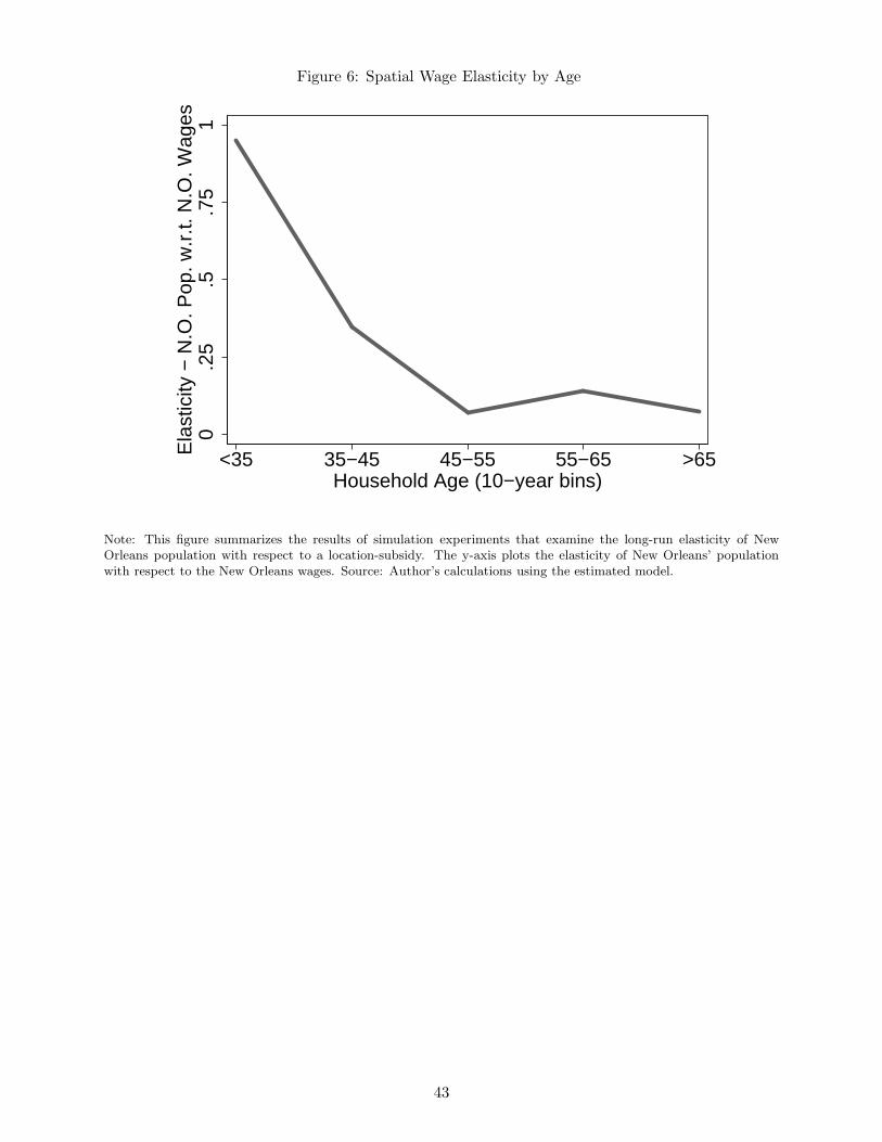
Figure 6: Spatial Wage Elasticity by Age

0.2

5.5

.75

1E

last

icity

− N

.O. P

op. w

.r.t.

N.O

. Wag

es

<35 35−45 45−55 55−65 >65Household Age (10−year bins)

Note: This figure summarizes the results of simulation experiments that examine the long-run elasticity of NewOrleans population with respect to a location-subsidy. The y-axis plots the elasticity of New Orleans’ populationwith respect to the New Orleans wages. Source: Author’s calculations using the estimated model.

43

(1)Composition

Solo male headed 17.3Solo female headed 29.6Couple headed 53.1

RaceEither head is black 57.6Neither head is black 42.4

Education of most educated headH.S. dropout 8.4H.S. graduate 17.8Some college 24.9Bachelor's degree or higher 48.9

Household age †Under 40 22.340-49 22.950-64 29.965 or older 25.0

Attachment to placeHome purchased > 25 years before Katrina 37.5Home purchased 10-25 years before Katrina 25.8Home purchased 0-10 years before Katrina 36.7

Either household head born outside of Louisiana 23.4Neither household head born outside of Louisiana 76.6

Pre-Katrina annual household income< $20,000 17.7$20,000 - $40,000 22.5$40,000 - $80,000 33.6> $80,000 26.3

Pre-Katrina home valueAppraised value less than $60k 31.9Appraised value between $60k and $120k 40.0Appraised value between $120k and $180k 9.9Appraised value more than $180k 18.3

Neighborhood povertyBlock group poverty rate (2000 Census), <10% 21.3Block group poverty rate (2000 Census), 10% - 25% 45.7Block group poverty rate (2000 Census), > 25% 32.7

Observations 560

Table 1. Household Background Characteristics

Note: This table reports the sample means of household background variables for the sample of pre-Katrina New Orleans households used to estimate the dynamic model. The sample includes only households that owned single-family homes (either free-and-clear or with a mortgage) at the time of Katrina. The sample also restricts attention to households in which at least one household head was employed during the year prior to Katrina or that had reached retirement age. Source: DNORS data and Assessor's data.

† Household age is defined to be the age of the male household head if present and the age of the female head otherwise.

44

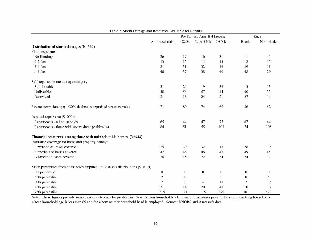
All households <$20k $20k-$40k >$40k Blacks Non-blacksDistribution of storm damages (N=560)Flood exposure

No flooding 26 17 16 31 11 450-2 feet 13 15 14 13 12 152-4 feet 21 31 32 16 29 11> 4 feet 40 37 38 40 48 29

Self-reported home damage categoryStill liveable 31 26 19 36 13 53Unliveable 48 56 57 44 60 33Destroyed 21 18 24 21 27 14

Severe storm damage; >30% decline in appraised structure value 71 80 74 69 86 52

Imputed repair cost ($1000s)Repair costs - all households 65 44 47 75 67 64Repair costs - those with severe damage (N=414) 84 51 55 103 74 108

Financial resources, among those with uninhabitable homes (N=414)Insurance coverage for home and property damage

Few/none of losses covered 25 39 32 18 28 19Some/half of losses covered 47 46 46 48 49 45All/most of losses covered 28 15 22 34 24 37

Mean percentiles from households' imputed liquid assets distributions ($1000s)5th percentile 0 0 0 0 0 025th percentile 2 0 1 2 0 550th percentile 7 3 4 10 2 1975th percentile 31 14 20 40 10 7895th percentile 219 101 145 275 101 477

Table 2. Storm Damage and Resources Available for Repairs

Pre-Katrina Ann. HH Income Race

Note: These figures provide sample mean outcomes for pre-Katrina New Orleans households who owned their homes prior to the storm, omitting households whose household age is less than 65 and for whom neither household head is employed. Source: DNORS and Assessor's data.

45

Property Holding / Payment Option 1 Option 2 or 3 SaleOwns Damaged Home or Receives Home's Market Value X X

Insurance Payment X X XRoad Home Grant (Repair Cost - Insurance Payment) † X X† Grant payment is 40% lower for option 3 participants

Group Option 1 Option 2 or 3 Private SaleNo R.H or

Sale TotalAll households with damaged homes 67 8 10 15 100

Not destroyed but uninhabitable 68 5 10 17 100Destroyed 75 14 6 5 100

Few/none of losses covered by insurance 78 12 2 9 100Some/half of losses covered by insurance 71 9 7 13 100All/most of losses covered by insurance 51 3 21 25 100

No flooding 0 0 18 82 1000-2 feet 60 0 15 25 1002-4 feet 75 5 8 12 100> 4 feet 68 12 9 11 100

<50% neighbors' homes uninhabitable 29 0 0 71 10050%-90% of neighbors' homes uninhabitable 53 8 11 29 100<50% neighbors' homes uninhabitable 71 8 10 11 100Observations 414

Program Participation --- Percent selecting various options among New Orleans homeowners with initially uninhabitable homes

Table 3. The Road Home Homeowner Program -- Program Benefits and Participation Patterns

Note: This table describes patterns of participation in the Road Home Homeowner program within the DNORS sample analyzed in this study. Road Home participants selected from three available reimbursement packages, known as options 1, 2, and 3. A household that selected option 1 received a grant payment equal to its estimated home-repair costs minus any private insurance payments and agreed to repair and reside in the home within three years of receiving the grant. A household that selected option 2 agreed to sell its home to a state land trust at a price equal to the grant that it would have been payed under option 1 and agreed to purchase another home in Louisianna within three years. A household that selected option 3 agreed to sell its home to a state land trust at a price equal to 60% of the grant that it would have been payed under option 1, but did not face any residency or home-purchase requirements.

Property Holding and Insurance/Grant

46

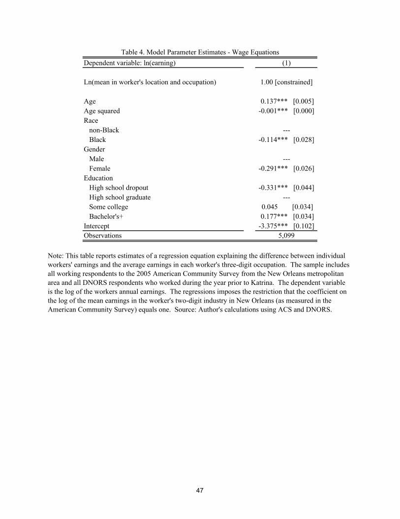
Dependent variable: ln(earning) (1)

Ln(mean in worker's location and occupation) 1.00 [constrained]

Age 0.137*** [0.005]Age squared -0.001*** [0.000]Race

non-Black ---Black -0.114*** [0.028]

GenderMale ---Female -0.291*** [0.026]

EducationHigh school dropout -0.331*** [0.044]High school graduate ---Some college 0.045 [0.034]Bachelor's+ 0.177*** [0.034]

Intercept -3.375*** [0.102]Observations 5,099

Note: This table reports estimates of a regression equation explaining the difference between individual workers' earnings and the average earnings in each worker's three-digit occupation. The sample includes all working respondents to the 2005 American Community Survey from the New Orleans metropolitan area and all DNORS respondents who worked during the year prior to Katrina. The dependent variable is the log of the workers annual earnings. The regressions imposes the restriction that the coefficient on the log of the mean earnings in the worker's two-digit industry in New Orleans (as measured in the American Community Survey) equals one. Source: Author's calculations using ACS and DNORS.

Table 4. Model Parameter Estimates - Wage Equations

47

(a) (b)Trend during first

five years following Parameter: Long run KatrinaFlow benefit from residence location - B(L)

Residence in a Southern metro area besides New Orleans -- B(3) 0.000 [ normalized]Residence in New Orleans -- B(2)

Intercept -0.068 [0.018]*** -0.148 [0.011]***

Residence in pre-Katrina home -- B(1)Intercept 0.577 [0.063]***Black -0.203 [0.057]***50%-90% of homes on the household's block segment uninhabitable -0.009 [0.096] 0.247 [0.036]***>90% of homes on the household's block segment uninhabitable 0.072 [0.054] 0.538 [0.074]***Block poverty rate (2000 Census), 10% - 25% -0.003 [0.093] Block poverty rate (2000 Census), > 25% 0.050 [0.059] Purchased home 10-20 years before Katrina -0.066 [0.048] Purchased home > 20 years before Katrina -0.135 [0.055]* Neither head born in Louisiana 0.002 [0.029]

Moving utility cost - χM

Move in the first period following Katrina 3.515 [0.037]***Moves after the first period 2.786 [0.067]***Additional cost to moves to or from New Orleans after the first period 1.240 [0.063]***Additional cost to moves in the first period following a home's repair -4.237 [0.098]***

Repairing/rebuilding cost - χR

Intercept 3.582 [0.120]***Additional utility cost to rebuilding a destroyed home 1.203 [0.019]***

Log of Borrowing interest rate - ln(1+rB)Intercept ln(1/β) [ normalized ]Black 0.141 [0.003]***No bachelor's degree 0.357 [0.011]***Annual household income before Katrina < $20,000 0.414 [0.015]***Annual household income before Katrina $20,000 to $40,000 -0.012 [0.003]***

Scale of shocks relative to u(c), α 5.047 [1.312] Scale of persistent unobserved heterogeneity, σ 0.647 [0.045]

Observations - household-periodsObservations - householdsLog-Likelihood

Table 5. Structural Parameter Estimates - Utility function and borrowing rate parameters

Note: This table reports nested fixed point maximum likelihood estimates of the model's structural parameters (see Section 6 for details). Assymptotic standard errors clustered at the neighborhood level are reported in brackets. Asterisks indicate statistical significance at confidence levels of (*) 5%, (**) 1%, and (***) 0.1% -- no *s are reported for the scale parameters. Source: Author's calculations using DNORS and Assessor's data covering calender years 2005 through 2009.

6,720560

-2,629.3

48

Moments - Percentage of households Data Model χ2 Data Model χ2 Data Model χ2 Data Model χ2

Home liveable1st Anniversary 30.7 32.6 0.06 22.7 22.6 0.00 21.2 25.7 0.57 36.7 38.1 0.022nd Anniversary 38.0 40.8 0.13 28.4 31.5 0.18 29.2 35.0 0.63 44.2 45.7 0.033rd Anniversary 47.7 53.4 0.78 30.7 46.5 4.26 36.5 49.0 2.97 56.7 57.1 0.004th Anniversary 69.6 66.3 0.56 67.0 61.7 0.81 67.2 63.8 0.25 71.3 68.5 0.34

Living in pre-Katrina home1st Anniversary 22.1 22.4 0.00 14.8 14.3 0.01 16.1 18.5 0.22 26.6 26.1 0.012nd Anniversary 29.1 29.7 0.01 21.6 21.9 0.00 23.4 26.4 0.22 33.4 33.1 0.003rd Anniversary 36.8 41.8 0.97 23.9 36.0 3.18 30.7 39.5 1.87 42.7 44.2 0.094th Anniversary 57.9 55.2 0.51 58.0 51.6 1.15 59.1 55.1 0.39 57.3 56.2 0.08

Living in New Orleans1st Anniversary 60.7 61.1 0.01 60.2 57.0 0.34 52.6 60.2 1.62 64.2 62.5 0.122nd Anniversary 71.4 71.3 0.00 71.6 68.1 0.57 67.2 71.3 1.32 73.1 72.2 0.043rd Anniversary 75.4 75.5 0.01 73.9 72.8 0.05 74.5 76.0 0.21 76.1 76.0 0.004th Anniversary 78.4 76.7 0.66 76.1 74.3 0.16 81.0 77.8 1.34 77.9 76.9 0.09

Sold pre-Katrina home1st Anniversary 3.2 4.8 4.12 2.3 5.8 4.68 1.5 4.5 9.02 4.2 4.7 0.182nd Anniversary 8.8 9.1 0.06 5.7 11.0 4.61 5.8 8.5 1.76 10.7 8.8 1.643rd Anniversary 16.1 12.8 4.64 11.4 15.4 1.28 13.9 11.9 0.39 18.2 12.4 11.784th Anniversary 19.6 15.9 4.15 19.3 19.1 0.00 15.3 14.9 0.02 21.5 15.5 7.13

Households 560 78 111 371

Moments - Percentage of households Data Model χ2 Data Model χ2 Data Model χ2 Data Model χ2

Home liveable1st Anniversary 6.3 8.9 1.26 6.9 6.7 0.00 3.6 9.1 6.16 7.4 9.5 0.462nd Anniversary 16.2 20.0 0.88 13.7 17.4 0.64 13.4 20.5 2.23 18.3 20.5 0.213rd Anniversary 29.2 37.0 3.50 16.4 35.5 11.47 22.3 37.6 7.77 36.7 37.2 0.024th Anniversary 58.9 54.4 1.32 60.3 53.8 0.99 59.8 55.7 0.31 58.1 53.9 1.34

Living in pre-Katrina home1st Anniversary 3.4 5.6 2.23 5.5 4.3 0.13 2.7 6.0 2.58 3.1 5.9 2.902nd Anniversary 11.8 13.6 0.34 11.0 12.2 0.09 9.8 14.2 1.19 13.1 13.7 0.053rd Anniversary 22.0 29.2 4.70 13.7 28.8 7.62 17.9 29.7 6.14 26.6 29.0 0.714th Anniversary 50.0 47.1 0.59 54.8 47.5 1.25 52.7 48.4 0.34 47.2 46.3 0.05

Living in New Orleans1st Anniversary 51.9 53.4 0.20 58.9 52.6 0.89 45.5 54.3 2.15 52.8 53.1 0.002nd Anniversary 65.7 65.5 0.00 69.9 64.8 0.95 61.6 66.7 2.05 66.4 65.2 0.063rd Anniversary 71.3 71.0 0.00 72.6 70.5 0.17 69.6 72.3 0.53 71.6 70.5 0.074th Anniversary 74.9 73.0 0.82 75.3 72.6 0.28 77.7 74.6 1.00 73.4 72.4 0.07

Sold pre-Katrina home1st Anniversary 2.4 5.4 12.63 0.0 6.2 - 0.9 4.9 21.12 3.9 5.3 1.262nd Anniversary 8.7 10.2 0.95 4.1 11.7 10.85 5.4 9.4 3.42 11.8 10.1 0.893rd Anniversary 17.4 14.2 2.87 9.6 16.3 3.20 15.2 13.1 0.34 21.0 14.1 11.024th Anniversary 21.3 17.6 3.02 19.2 20.1 0.04 16.1 16.3 0.01 24.5 17.5 7.26

Households 414 66 91 257

0k < HH Income < $4 HH Income > $40k

Table 6. Model Fit

All Households HH Income < $20k 0k < HH Income < $4

Note: This table compares the value of various sample moments to the model's predicted value for those moments. For each comparison, a cluster-robust chi-squared test stratistic (clustered at the neighborhood level) is reported for a test of the null that the predicted and empirical moments are equal. The critical value for the chi-squared(1) distribution with alpha=0.05 is 3.84.

All HouseholdsHH Income > $40k

Among Households with an Initially Damaged HomeAll Households HH Income < $20k

49

(1) (2) (3) (4) (5) (6) (7) (8)

GroupNo Grant Program

Road Home

ProgramNo Grant Program

Road Home

ProgramNo Grant Program

Road Home

ProgramNo Grant Program

Road Home

Program

All Households 49.0 54.4 42.7 47.1 70.8 73.0 19.9 17.6

Household Income:< $20k 43.7 53.8 38.6 47.5 69.2 72.6 22.9 20.1Between $20k and $40k 49.5 55.7 43.4 48.4 72.4 74.6 18.9 16.3> $40k 50.4 53.9 43.7 46.3 70.6 72.4 19.4 17.5

Race:Black 49.4 55.8 43.7 48.9 73.2 75.7 17.7 15.4Non-black 48.0 51.2 40.5 43.1 65.8 67.1 24.7 22.5

Insurance coverage:Few/none of losses covered 43.8 53.7 39.0 47.5 68.6 73.4 21.3 17.8Some/half of losses covered 46.3 52.2 40.7 45.2 69.9 71.9 21.2 18.5All/most of losses covered 58.1 58.8 49.4 49.9 74.4 74.5 16.5 16.1

Other illustrative subgroups:HH income < $20k & few/none of losses covered by insurance 43.1 58.1 39.3 53.0 69.5 75.9 20.6 17.0Bachelor's degree and all/most of losses covered by insurance 56.9 58.0 47.3 48.4 72.7 72.9 17.8 17.1

Table 7. The Impact of the Road Home Program on Resettlement Choices and Welfare

Note: This table provides the results of simulation experiments designed to assess the partial equilibrium impact of the Road Home program. The first four pairs of columns (columns 1-8) report pairs of simulated outcomes, the first of each pair reporting the outcome under a scenario in which no Grant Program was in place and the second reporting the outcome under the scenario in which the Road Home program was available. The final columns (column 9) computes the Road Home program's impact households' expected welfare. Expected welfare is computed at time t=0. For each household, welfare in the scernario in which no grant program is in place is normalized to zero . For each household, expected welfare under the scenario in which all home repairs not covered by insurance are reimbursed at t=0 is defined to by one hundred. The welfare impact of the Road Home program is reported as a fraction of the welfare impact of immediate full reimbursement. Source: Author's calculations using the estimated model.

Living in New Orleans

Home Repaired by Original Owner

Living in pre-Katrina Home Sold Home

Resettlement Outcomes -- Measured on Katrina's 4th Anniversary

50

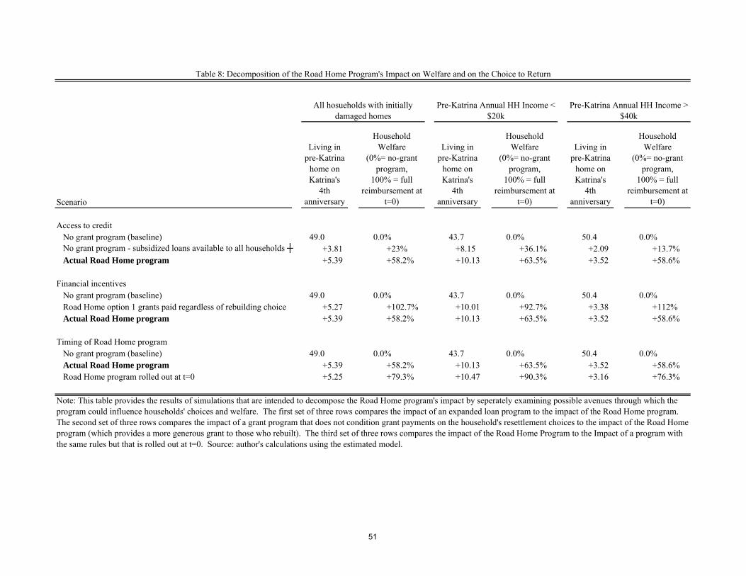
Scenario

Living in pre-Katrina

home on Katrina's

4th anniversary

Household Welfare

(0%= no-grant program,

100% = full reimbursement at

t=0)

Living in pre-Katrina

home on Katrina's

4th anniversary

Household Welfare

(0%= no-grant program,

100% = full reimbursement at

t=0)

Living in pre-Katrina

home on Katrina's

4th anniversary

Household Welfare

(0%= no-grant program,

100% = full reimbursement at

t=0)

Access to creditNo grant program (baseline) 49.0 0.0% 43.7 0.0% 50.4 0.0%No grant program - subsidized loans available to all households ┼ +3.81 +23% +8.15 +36.1% +2.09 +13.7%Actual Road Home program +5.39 +58.2% +10.13 +63.5% +3.52 +58.6%

Financial incentivesNo grant program (baseline) 49.0 0.0% 43.7 0.0% 50.4 0.0%Road Home option 1 grants paid regardless of rebuilding choice +5.27 +102.7% +10.01 +92.7% +3.38 +112%Actual Road Home program +5.39 +58.2% +10.13 +63.5% +3.52 +58.6%

Timing of Road Home programNo grant program (baseline) 49.0 0.0% 43.7 0.0% 50.4 0.0%Actual Road Home program +5.39 +58.2% +10.13 +63.5% +3.52 +58.6%Road Home program rolled out at t=0 +5.25 +79.3% +10.47 +90.3% +3.16 +76.3%

Note: This table provides the results of simulations that are intended to decompose the Road Home program's impact by seperately examining possible avenues through which the program could influence households' choices and welfare. The first set of three rows compares the impact of an expanded loan program to the impact of the Road Home program. The second set of three rows compares the impact of a grant program that does not condition grant payments on the household's resettlement choices to the impact of the Road Home program (which provides a more generous grant to those who rebuilt). The third set of three rows compares the impact of the Road Home Program to the Impact of a program with the same rules but that is rolled out at t=0. Source: author's calculations using the estimated model.

Table 8: Decomposition of the Road Home Program's Impact on Welfare and on the Choice to Return

All hosueholds with initially damaged homes

Pre-Katrina Annual HH Income < $20k

Pre-Katrina Annual HH Income > $40k

51

Group -- among population of working-aged householdsHome repaired by pre-Katrina owner by

Katrina's fourth Anniversary

All households with home damage not covered by insuranceActual policy environment 57.601Direct grant reduced by $2,400 -0.056Present value of New Orleans wages $2,400 lower -0.027

Households with pre-Karina annual income < $20kActual policy environment 59.017Direct grant reduced by $2,400 -0.188Present value of New Orleans wages $2,400 lower -0.039

Households with pre-Karina annual income > $40kActual policy environment 57.465Direct grant reduced by $2,400 -0.043Present value of New Orleans wages $2,400 lower -0.032

Table 9: The Relative Impact of Direct Grants and Similarly Sized Wage Subsidies

Note: This table provides the results of simulation experiments designed to assess the relative impact of direct grants and similarly sized wage subsidies on households' resettlement choices. These experiments restrict attention to working age households (head < 65 years old). For each set of results (three-row groups), the first row provides the fraction of homes repaired by the pre-Katrina owner under a baseline simulation that imposed the actual post-Katrina policy environment. The second row provides the impact of removing $2,400 per worker from the size of each household's Road Home option 1 grants. The third row provides the impact of removing $2,400 per worker from the present value of New Orleans labor wages (spread evenly over the first four years following Katrina). Source: author's calculations using the estimated model.

52

Spatial elasticity used in DWL calculation: Per-year probability of a disaster: 1/50 1/30 1/50 1/30 1/50 1/30

Baseline value of housing stock $11 B $11 B $11 B $11 B $11 B $11 BSubsidy's flow expcted value, as a fraction of home value (τ ) 2.00% 3.30% 2.00% 3.30% 2.00% 3.30%Elasticity: ψ = dln(N.O. homeowners) / d[ flood insurance subsidy (τ) ] 0.450 0.450 0.450 0.450Elasticity: ψ among young households 1.737 1.737 1.737 1.737

Flow cost of subsidy ( [ Value of Housing Stock] • τ ) $220 M $363 M $220 M $363 M $220 M $363 M

Deadweight loss ( ≈ 1/2 • [ Value of Housing Stock] • ψ • τ2 ) $1 M $2.7 M $1.7 M $4.6 M $3.8 M $10.4 M

Note: This table provides the quantities necessary to compute the deadweight loss associated with a hypothetical flow subsidy to residence in New Orleans. Sources: The baseline value of the New Orleans housing stock is computed from Orleans Parish Property Assessment data. The semi-elasticity of the New Orleans homeowning population with respect to a flow subsidy to residence in New Orleans (an annual subsidy as a fraction of a household's home's value) is computed using simulations with the estimated model. The quantity labeled average households' elasticity is computed using the change in the fraction of simulated panels for all model households in which the household is living in New Orleans eight years after Katrina. The quantity labeled young households' elasticity is computed using a similar calculation among houeholds that were age 35 or less when Katrina occurred.

Table 10: The Deadweight Loss Associated with a Flow Subsidy to Flood Insurance

Young Households' ElasticityAverage Households' Elasticity75% Average Households' Elasticity25% Young Households' Elasticity

53

Variable Description Method Data sourceMonthly mortgage payment for pre-Katrina home

Mortgage payment associated with a standard 30 year fixed rate mortgage

Computed using home's purchase date and purchase price assuming a thirty year fixed rate mortgage with a 20% down payment

-Assessor's data

Monthly rent for a different New Orleans residence

Estimate of the cost of renting housing that is comparable to the household's pre-Katrina home

Step 1: impute the home's rental value in pre-Katrina New Orleans 0.0785 x (appraised pre-Katrina value) / 12.Step 2: adjust that for differences in rental prices between pre-Katrina New Orleans and post-Katrina New Orleans using regression adjusted price indeces (see Appendix II for details on computing rental price indices)

-Pre-Katrina appraised home values come from Assessor's data-Housing price indices are computed using information on rental prices and building characteristics from the American Community Survey

Monthly rent for a residence in another Southern metro

Estimate of the cost of renting housing that is comparable to the household's pre-Katrina home

Step 1: impute the home's rental value in pre-Katrina New Orleans 0.0785 x (appraised pre-Katrina value) / 12.Step 2: adjust that for differences in rental prices between pre-Katrina New Orleans and the post-Katrina market in other Southern metro areas using regression adjusted price indeces (see Appendix II for details on computing rental price indices)

-Pre-Katrina appraised home values come from Assessor's data-Housing price indices are computed using information on rental prices and building characteristics from the American Community Survey

Cost of repairing home damage Estimate of the cost of repairing the household's home if the home was damaged but not destroyed, and an estimate of the cost of rebuilding the household's home if it was destroyed

-If home was destroyed, repair cost is imputed to be the appraised pre-Katrina improvement value multiplied by a price index that reflects the difference in housing prices between pre-Katrina and post-Katrina New Orleans (this assumes that post-Katrina housing prices more accurately reflect building costs than pre-Katrina prices (Vigdor, 2008))-If home was uninhabitable but not destroyed, repair cost is imputed to be the difference between the appraised pre-Katrina improvement value and the appraised improvement value immediately following Katrina multiplied by a price index that reflects the difference in housing prices between pre-Katrina and post-Katrina New Orleans

-Appraised home values come from Assessor's data-Housing price indices are computed using information on rental prices and building characteristics from the American Community Survey

Insurance payment Estimate of the insurance payment made to the household to cover damage to the household's home

Imputed by multiplying the household's repair costs by a fraction based on the household's categorical response to the DDNORS question asking what fraction of losses were covered by insurance (all or almost all, 1.0; most, 0.75; about half, 0.5; some 0.25; very few, none, or had no insurance, 0.0)

-DNORS

Sale price of pre-Katrina home if it is repaired

Estimate of the price at which the household's home would sell following Katrina if it were fully repaired

Imputed by multiplying the home's appraised pre-Katrina value by an estimated price index reflecting the difference in housing prices between pre-Katrina and post-Katrina New Orleans

-Pre-Katrina appraised home values come from Assessor's data-Housing price indices are computed using information on rental prices and building characteristics from the American Community Survey

Table A1. Constructing Housing-Related Price Variables

54

(1) (2)

Housing Market IndicatorsPre-Katrina New Orleans --- ---Post-Katrina New Orleans 0.383*** [0.015] 0.352*** [0.015]Elsewhere in Metro South 0.333*** [0.014] 0.233*** [0.013]

Constant 6.142*** [0.013] 6.142*** [0.013]Controls for building characteristics: centered around 2005 New Orleansmeans (X i-X bar)

No Yes

Observations 706,073 706,073

Table A2. Housing Price Index Regressions

Note: These regressions were computed using all renting households that lived in the New Orleans MSA in 2005-2009 or in another Southern metro from 2006-2009. The estimates were computed by regressing the log of rent on a constant, an indicator that an observation came from post-Katrina New Orleans, an indicator that an observation came from another southern metro, and (in the second column) a set of building characteristic variables centered around their mean values in the 2005 New Orleans sample. The housing market dummies should be interpreted as the mean difference in the log of rents between the indicated housing market and pre-Katrina New Orleans. Source: American Community Survey.

55

Uninhabitable butFlood exposure Still inhabitable not destroyed Destroyed Total Still inhabitable Uninhabitable Total

No flooding 92 8 0 100 84 16 1000-2 feet 31 60 9 100 24 76 1002-4 feet 11 69 19 100 4 96 100> 4 feet 1 59 39 100 0 100 100

Observations 560 560

Self-reported home damage Measure based on property appraisals

Note: this table describes the relationship between the depth of flooding on a household's block and the damage to the household's home. Source: flood depth comes from maps produced by FEMA. Self reported home damage comes from DNORS interviews. The property appraisal based measure classifies a property as uninhabitable if its appraised improvement value declined by more than 30% from the last appraisal prior to Katrina to the first appraisal after Katrina (conducted during the Fall of 2005).

Table A3. Distribution of Storm Damage by Flood Exposure

56

Date EventAugust 27, 2005 • New Orleans Mayor Ray Nagin announces a state of emergency and

suggests a voluntary evacuation of the city.

August 28, 2005 • Mayor Nagin announces a mandatory evacuation of New Orleans, and the Louisiana Superdome is opened as a refuge for those unable to leave the city.

August 29, 2005 • Hurricane Katrina makes landfall on the Gulf coast.

August 29, 2005 • President George W. Bush declares much of the Gulf coast (including New Orleans) to be a major disaster area. This designation allows residents who suffer storm-related damages to seek assistance through standing federal disaster relief programs, such as FEMA's Disaster Assistance Grants and SBA's Disaster Assistance loans.

September 6, 2005 • Mayor Nagin orders a forced evacuation of New Orleans, and National Guard troops enter the city to enforce the order. The city's population of pre-storm residents falls to nearly zero, from the pre-storm level of about 460,000.

September 28, 2005 • Residents of least damaged areas of the city are first permitted to return, but, with few city services yet restored, very few return this early.

December 17, 2005 • Congress passes the Gulf Opportunity Zone initiative into law.

February 20, 2006 • Louisiana officially announces the Road Home rebuilding grant program .

March 2, 2007 (week of) • The first Road Home rebuilding grant is paid to a New Orleans homeowner.

July 31, 2007 • The deadline for submitting Road Home grant applications occurs.

December 7, 2007 (week of) • About 32,000 Road Home grants have been paid to New Orleans homeowners, about 75% of the total number of grants eventually dispersed.

Table A4: Post-Katrina Policy Timeline

57