Embed Size (px)
Citation preview

THE IMPACT OF PULL SYSTEM
STRUCTURE AND CONFIGURATION
ON PRODUCTION LINE PERFORMANCE
UNDER STATE DEPENDENT BEHAVIOR
Master’s Thesis
By:
Hariadhi Wicaksono
Student number: S2699338
MSc Technology & Operations Management
University of Groningen, Faculty of Economics and Business
2015

i
Abstract
Purpose: Pull system design is defined by its structure and configuration, which are the
pattern of work in process limit and the level of the work in process (WIP) limit, respectively.
WIP limitation allows the occurrence of starving and blocking in the production system,
where experimental evidence shows that human workers adjusts their work processing time to
minimize the occurrence of starving and blocking. This processing time adjustment behavior,
referred to as the state-dependent behavior, is incorporated into the study of pull system
structure and configuration to analyze their effect on line performance. By studying
simulation models, this research aims to provide a more accurate understanding in designing
an efficient pull system with human workers.
Method: A pull system production line simulation model is made by incorporating a state-
dependent behavior model made by Powell and Schultz (2004) and a pull system design
model made by Gaury, Kleijnen, and Pierreval (2001). Different pull system structures and
pull system configurations are used as the experimental input for the simulation study to
analyze the relation between pull system structures and pull system configurations to line
performance under the influence of state-dependent behavior.
Findings: Increasing the occurrence of workflow disturbance through the pull system
structure increases the system throughput. Increasing the pull system configuration also
increases throughput, but with a diminishing rate of throughput increase.
Pull system structure under state-dependent behavior alters the initially balanced work
allocation pattern into an imbalanced allocation pattern. This occurrence increases the
throughput of the production line further when the higher workloads are distributed to the
workstation with faster average processing time and the lower workloads on the slower
workstations. In extended production lines, throughput decrease from higher stochastic
interference is minimized under state-dependent behavior due to more interior workers that
have faster processing times.
Recommendations: There are various possible pull system structures that can be studied
under state-dependent behavior, which might have a better cost efficiency than the
performance of the Kanban, POLCA, or CONWIP pull system structure.
Further development of the state-dependent behavior model should be done to incorporate the
diminishing awareness from increasing buffer capacity.

ii
Preface
This project is the final project that is done to obtain my Master of Science in Technology and
Operations Management degree. This project incorporates the principle of the program itself
by practicing how efficiency in a system can be attained through an appropriate management
of both technology and human who run the operation.
The objective of the project is to understand the two most important parts of a pull system
design, that is the structure and the configuration that implements limitation of work in
process in the production system. The result of the simulation study achieves the objective of
the study as well as providing new insights and interests for both operation management
practitioners and researchers.
I would like to thank my supervisor for his patience and continuous effort in providing
reviews and feedbacks throughout the project. Without his help in building the code, as well
as providing a facility to run the simulation, I could not finish the simulation on time.
I would also like to thank my co-assessor for his input on the initial stage of the project. I also
want to give the most gratitude to my fellow Technology and Operations Management master
students for providing me feedbacks during the initial poster presentation and final
presentation, especially to those who personally helps me with the writing of the report.
Finally, I thank every single person that has given me the knowledge and support up to this
point, so that I could finish this project in time.
Groningen, June 2015

iii
TABLE OF CONTENTS
1 Introduction .............................................................................................................. 1
2 Theoretical Background ........................................................................................... 3
2.1 State-Dependent Behavior ................................................................................ 3
2.2 Pull System Structure and Configuration ......................................................... 5
2.3 How Structure and Configuration Contributes to State-Dependent Behavior .. 7
2.4 Conceptual Model ............................................................................................. 7
3 Methodology ............................................................................................................ 8
3.1 Production Line Model ..................................................................................... 9
3.2 State-Dependent Behavior Model ..................................................................... 9
3.3 Simulation Program ........................................................................................ 10
4 Simulation .............................................................................................................. 11
4.1 Model Summary ............................................................................................. 11
4.2 Simulation Setup ............................................................................................. 14
4.3 Simulation Model Validation ......................................................................... 15
4.4 Simulation Result............................................................................................ 16
4.4.1 Structure, Configuration, and Speedup Constant ...................................... 16
4.4.2 Structure, Configuration, and Work Allocation ........................................ 18
4.4.3 Structure, Configuration, and Line Length ............................................... 20
5 Discussion .............................................................................................................. 22
5.1 Pull System Configuration .............................................................................. 22
5.2 Pull System Structure ..................................................................................... 23
5.3 Work In Process .............................................................................................. 25
6 Conclusion ............................................................................................................. 26
6.1 Conclusion ...................................................................................................... 26
6.2 Recommendations ........................................................................................... 27
6.3 Limitations and suggestions for future research ............................................. 28

iv
References .................................................................................................................... 29
APPENDIX A : WIP Movement Flowchart ................................................................ 31
APPENDIX B: Workers processing time adjustment model ....................................... 32
APPENDIX C: Warm-Up length, Replication, and Run Length ................................. 33
APPENDIX D: Summary of Simulation Result ........................................................... 37
3 Workstations: Throughput ..................................................................................... 37
3 Workstations: Average Cycle Time ....................................................................... 38
3 Workstations: Average WIP .................................................................................. 39
5 Workstations: Throughput ..................................................................................... 40
5 Workstations: Average Cycle Time ....................................................................... 41
5 Workstations: Average WIP .................................................................................. 42
TABLE OF FIGURES
Figure 2.1 Kanban pull system structure (Ziengs et al., 2012) ...................................... 6
Figure 2.2 CONWIP pull system structure (Germs and Riezebos, 2009) ...................... 6
Figure 2.3 POLCA pull system structure (Germs and Riezebos, 2009) ........................ 6
Figure 2.4 Conceptual Model of the Study .................................................................... 7
Figure 4.1 Generic pull system structure (Gaury, Kleijnen, and Pierreval, 2001) ....... 12
Figure 4.2 Efficiency On Different Speedup Constants ............................................... 15
Figure 4.3 Efficiency of each structure on increasing configuration ........................... 16
Figure 4.5 Production line efficiency under different work allocation pattern ............ 18
Figure 4.6 Efficiency on Different Line Lengths ......................................................... 20
Figure 5.1 Efficiency on excessively higher pull system configurations ..................... 22
Figure 5.2 Average Processing Times and Average WIP ............................................ 24
Figure.Appendix 1 WIP Movement Flowchart ............................................................ 31
Figure.Appendix 2 Processing time adjustment flowchart .......................................... 32
Figure.Appendix 3 Welch’s Method Calculation Result for 3 Workstations .............. 33
Figure.Appendix 4 Run Length Calculation Graph for 3 Workstations ...................... 34
Figure.Appendix 5 Welch’s Method Calculation Result for 5 Workstations .............. 35
Figure.Appendix 6 Run Length Graphical Method Graph for 5 Workstations ............ 36

v
TABLE OF TABLES
Table 4.1 Model summary ............................................................................................ 11
Table 4.2 Worker processing time for different line length ......................................... 13
Table 4.3 Efficiency of different structures under the same maximum WIP ............... 17
Table 4.4 Efficiency of different structures under the same maximum WIP ............... 19
Table 5.1 Average WIP With Equal Level Of Maximum WIP ................................... 25
Table 5.2 Production Line Efficiency Relative to Their Average WIP ....................... 26
Table.Appendix 1 Confidence Interval Calculation Result for 3 Workstations ........... 33
Table.Appendix 2 Run Length Calculation Result for 3 Workstations ....................... 34
Table.Appendix 3 Confidence Interval Calculation Result for 5 Workstations ........... 35
Table.Appendix 4 Run Length Calculation Result for 5 Workstations ....................... 36
Table.Appendix 5 Throughput of each simulation in 3 workstation setting ................ 37
Table.Appendix 6 Average cycle time of each simulation in 3 workstation setting .... 38
Table.Appendix 7 Average WIP of each simulation in 3 workstation setting ............. 39
Table.Appendix 8 Throughput of each simulation in 5 workstation setting ................ 40
Table.Appendix 9 Average cycle time of each simulation in 5 workstation setting .... 41
Table.Appendix 10 Average cycle time of each simulation in 5 workstation setting .. 42

1
1 Introduction
Studies in operations management categorized the production systems into push and
pull production systems. A pull system is a production system that explicitly limits the
amount of work in process (WIP) in the system (Hopp & Spearman 2004). WIP can be
limited through the structure and the configuration of the pull system (Gaury, Pierreval &
Kleijnen 2000).The pull system structure is the specific pattern of control loops that regulates
the workload on a certain area in the production line, while pull system configuration is the
WIP limit in each of the control loops (Germs & Riezebos 2009).
By maintaining the level of WIP, pull systems can perform more efficiently compared
to push systems (Hopp & Spearman 2004). This advantage has triggered both practitioners
and researchers to tailor pull system designs for specific kinds of manufacturing conditions
(Hopp & Spearman 2008). This has resulted in several types of pull system structures such as
CONstant Work In Process or CONWIP (Spearman et al. 1990) and Paired-cell Overlapping
Loops of Cards or POLCA (Krishnamurthy & Suri 2009). Gaury, Pierreval and Kleijnen
(2000) study the performance of various pull system designs by simulating a generic pull
system design that incorporates any possible types of pull system structure and pull system
configuration. They concluded that the CONWIP structure leads to better performance
compared to other pull system structures.
Pull system structure and pull system configuration are known to critically affect the
performance of the pull system (Khojasteh-Ghamari 2009). Coupling, a workflow disturbance
caused by starving and blocking of the buffer, is operationalized by the pull system structure
and configuration (Heimbach, Grahl & Rothlauf 2012). A tightly coupled pull system strictly
limits WIP which causes higher occurrence of starving and blocking. On the other hand, a
loosely coupled pull system like CONWIP, allows more WIP in the system to prevent
starving and blocking.
Past research generalizes that a pull system has a smaller production rate compared to
a push system due to the WIP limiting mechanism (Doerr et al. 1996). This conclusion,
however, may not be true for production lines with human workers since humans do not
behave independently of the situation around them (Schultz et al. 1998). Empirical studies
have shown that blocking and starving of the buffer made the workers adjust their processing
time, according to the state of the buffer and the speed of their co-workers (Doerr et al. 1996;
Schultz et al. 1998).

2
The workers processing time adjustment are strengthened in lower pull system
configurations because starving and blocking is more likely to happen, and workers adjust
their processing time to avoid this to happen (Schultz, Juran & Boudreau 1999). These studies
show that pull systems could benefit from the response of production workers to the state of
their production line and that performance deterioration has been overstated.
Powell and Schultz (2004) coined the term state-dependent behavior to define the
workers processing time adjustment behavior that opposes the independence assumption. In
their paper which examines the effect of state-dependent behavior on line performance and
line length, they mention that other aspects of line design would be a promising extension for
research in state-dependent behavior. Heimbach, Grahl, and Rothlauf (2012) extend the state-
dependent behavior research by including work allocation in their experiment. Both of the
literatures conclude that a tightly coupled production system benefits more from state-
dependent behavior rather than a loosely coupled system. This effect caused the state-
dependent pull system to outperform the state-independent push system that has no
interference from the coupling.
This is surprising because the studies in pull system structure and pull system
configuration suggest that the loosely coupled pull system design results in better line
performance, while studies in state-dependent behavior suggest the opposite. It is intriguing to
see how state-dependent behavior will alter the performance of various pull system structures
and pull system configurations with different degrees of coupling. This interest leads to the
following research question.
RQ: What is the impact of pull system structure and configuration on line
performance given state-dependent behavior?
Based on the research question, this study aims to provide a better understanding to
design an efficient pull system with human workers. The analyses are based on the line
performance of different pull system structures and pull system configurations that are
compared to the performance of a state-independent push system as the reference point.
In the end, this study contributes in several ways. In operations management literature,
the research provides a complete initial model to study various possible pull system structures
and pull system configurations under the state-dependent behavior. More importantly, this

3
study facilitates practitioners with a practical tool to explore the suitable pull system structure
and pull system configuration according to their individual cases.
2 Theoretical Background
2.1 State-Dependent Behavior
Relation between workers’ processing time and their workload has been studied for
decades. Edie (1954) studied service times of toll booths and found that workers work faster
when the queue is longer, while Franks and Sury (1966) shows that workers in conveyor work
adjust their processing time according to the pace of arrival times. The interests to study state-
dependent behavior continues to develop and extended to the retail industry, such as the
service speed of restaurant workers and amount of tables being served (Tan and Netessine,
2014), or the service times of checkout in retails and the queue design (Shunko, Niederhoff
and Rosokha 2014). However, this state-dependent behavior effect has more complexity in a
serial production line where the workers processing time is affected by both his/her own
workload and the workload of the subsequent workstation.
Because of the WIP limit, a pull system buffer can be starved or blocked. A station
becomes starved when it cannot work because there is no inventory in the upstream buffer,
and it becomes blocked when it cannot work because there is no space to put the finished
goods in the downstream buffer. The lower the WIP limit in the system, the higher the
probability of workflow disturbance from starving and blocking. Meanwhile, push system can
never experience blocking because it does not implement a WIP limit.
The study of Doerr et al. (1996) is the first to determine the relation of the states of the
production line to the behavior of the workers. The result of their experiment on comparing
unlimited inventory push system and the low inventory pull system shows that both
production systems result in similar processing rates, even though there are more interruptions
in the lower inventory pull system. They conclude that the workers put more effort when they
are in producing state, since they experience short breaks from the starving and blocking
occurring in the pull system.
Schultz et al. (1998) extends the research on state-dependent behavior, aiming to
clarify the effect of the production workers processing time adjustment to the state of the
production line. They argue that the assumption of human workers behaving independently of
the state of the buffer, or the independence assumption, might not be true in low inventory

4
settings. They show that the assumption does not hold, by providing concrete empirical
evidences of state-dependent behavior in the result of their study. This result sheds a new light
in the study of behavioral operations management, especially, on the fact that workers speed
up if others are starving and slow down if they are about to starve.
Having clear evidence on the effect of state-dependent behavior in pull production
systems, the focus of the studies shifted to the design of the pull production system line.
Powell and Schultz (2004) pioneered this by exploring the relation between throughput and
the length of the serial line. They modeled the effect of state-dependent behavior in processing
time adjustment through a speedup constant. This speedup constant mechanizes the
adjustment of processing times by decreasing it according to the state of the adjacent buffers.
Their study shows that state-dependent behavior causes the increase of production line
performance along with the increase in line length under high level speedup constant. This
result shows contradiction with the classic assumption where line performance deteriorates
when the production line is extended.
Empirical evidences on state-dependent behavior, encourage researchers to explore its
implication on practical settings, especially in the design of a production system. Heimbach,
Grahl, and Rothlauf (2012) take this chance to explore the different work allocations of the
serial line. Through a similar method to those of previous studies, they model the effect of
state-dependent behavior on the adjustment of workers processing time in different types of
work allocations, line length, and buffer size. Their conclusion adds more evidence that shows
that state-dependent behavior affects the production rate positively by minimizing interruption
in the production line.
These studies by Powell and Schultz (2004) and Heimbach, Grahl and Rothlauf (2012)
experimented with the design of serial production lines. However, none of their experiment
focused on pull system structure and pull system configuration. As has been mentioned
earlier, the performance of a production line is critically related to the pull system structure
and pull system configuration, since they define the coupling level of the production line. It is
important to study the impact of state-dependent behavior on pull systems with different
coupling levels to have a better understanding of creating a more efficient production line
with human workers.

5
2.2 Pull System Structure and Configuration
Germs and Riezebos (2010) define the structure of the pull system as the pattern of
control loops among the production line where the movement of the WIP is regulated by a
certain limit, while the configuration of the pull system is the number of cards which limits
the amount of the WIP within the control loop. The basic pull production system, namely the
Kanban system, used two types of cards to define that the WIP attached with the card has to
be moved or has to be operated (Sugimori et al. 1977). Different types of card-based pull
system are distinguished by their unique placement of control loops and the number of cards
within the control loops in the production line (Gaury, Kleijnen & Pierreval 2001).
Pull system structure and pull system configuration defines the coupling level of a pull
system. A tightly coupled pull system strictly limits WIP by having a structure with less
workstations in each control loop and low configuration level in each control loop, inducing
higher likelihood of starving and blocking. A loosely coupled pull system has less chance of
blocking due to a larger area of control loops and high configuration level in each control
loop.
In the following section, three pull system structures with different coupling levels are
explained. The first one, Kanban, represents the tightly coupled pull system. CONWIP
represents the loosely coupled pull system since it has a structure that disables blocking and
starving except for the first and last workstations. Lastly, POLCA represents the pull system
design that has moderate coupling level, combining the benefit of Kanban and CONWIP. The
behaviors of these structures are used as main examples to study various pull system
structures and configurations that are generated by the generic pull system design (Gaury,
Pierreval & Kleijnen 2000).
The Kanban system has the goal to objectify the Just In Time (JIT) production, which
is a production of parts of the various processes in the necessary amounts at necessary timing
(Sugimori, et al. 1977). The structure of the Kanban system consists of a single station and the
subsequent buffer, creating a control loop in each stage of the production line, depicted in
figure 2.1 (Ziengs et al., 2012). This creates an inventory limit on each stage of the production
line. Compared to CONWIP, Kanban performs better in WIP minimization when processing
times between stations are close to balanced (Khojasteh-Ghamari, 2009).

6
CONstant Work In Progress (CONWIP) is a pull system structure that intends to
combine the advantage of Kanban in minimizing inventory and the throughput maximization
of push production systems (Spearman et al., 1990). This characteristic is operationalized by
the use of cards, in which the control loop structure consists of the entire production line. This
way, the configuration of the cards applies to the whole production line, as shown in figure
2.2 (Germs & Riezebos 2009). Compared to Kanban, CONWIP performs better in inventory
minimization when processing times between stations are imbalanced (Khojasteh-Ghamari,
2009).
Paired-cell Overlapping Loops of Cards with Authorization (POLCA) is a pull system
structure that claims the best features of card-based pull systems and push systems
(Krishnamurthy & Suri 2009). Different from CONWIP, the structure of POLCA covers the
entire line with several different control loops that overlap each other, presented in figure 2.3
(Germs & Riezebos 2010). The fundamental difference between POLCA and other card-based
pull system policies is that the card used in POLCA does not represent a request to operate a
product, but a signal representing available capacity at a downstream loop.
Figure 2.1 Kanban pull system structure (Ziengs et al., 2012)
Figure 2.2 CONWIP pull system structure (Germs and Riezebos, 2009)
Figure 2.3 POLCA pull system structure (Germs and Riezebos, 2009)
Gaury, Pierreval and Kleijnen (2000) initiated the first effort to produce a generic pull
production control policy. In order to find the optimal pull system design, they created a
generic structure that is able to represent all possible pull system structures. Through a

7
simulation study, they concluded that the loosely coupled CONWIP is the best pull system
structure in general.
2.3 How Structure and Configuration Contributes to State-Dependent Behavior
None of the past studies in state-dependent behavior has considered the pull system
structure and pull system configuration in their experiment (Powell & Schultz 2004;
Heimbach, Grahl & Rothlauf 2012). In state-independent serial line with stochastic processing
times, the loosely coupled CONWIP is generally deemed as the best strategy among other pull
systems considering its performance in maintaining service level and minimizing inventory
(Gaury, Pierreval, & Kleijnen 2001). However, loose coupling leads to less interdependence
between the workers who interact through the production line and weakens the awareness of
the workers to adjust their processing time. This causes CONWIP to have little benefit from
state-dependent behavior, while Kanban has the most benefit.
2.4 Conceptual Model
The conceptual model (Figure 2.4) describes the framework of the study. To
incorporate the interest of understanding the manner of state-dependent behavior under
different pull system structures and pull system configurations, a model is built for the
simulation. The magnitude of the state-dependent behavior in the model is represented by a
speedup constant, a mechanism that represents the processing time adjustment of workers
under state-dependent behavior (Powell & Schultz 2004). This speedup constant is embedded
in a mathematical function that changes the processing time of a worker, according to the state
of the upstream and the downstream buffer (Heimbach, Grahl & Rothlauf 2012).
Pull System Structure and Configurations
Line Performance
State of Production :Blocked, About to be blocked,
Producing, About to be starved, Starved
Model
· Speed-up Constant· Line Length· Structure and
Configuration· Work Allocation Pattern
· Efficiency
Figure 2.4 Conceptual Model of the Study
8
The experiment also includes line length and work allocation pattern as part of the
experimental inputs. Conway et al. (1988) claims that longer line length in a pull system
suffers from increasing stochastic interference which leads to a reduced throughput, which is
later shown to be not true in a state-dependent pull system model with high level of speedup
constant (Powell & Schultz 2004). Hillier and Boling (1979) define a ‘bowl’ shaped work
allocation pattern that allocates slower processing time at the first and the last workstation in a
serial production line, which works better than a balanced production line. Heimbach, Grahl
and Rothlauf (2012) studied the effect of the bowl pattern, reverse bowl pattern, and the
balanced pattern under state-dependent behavior and found that each pattern increases line
performance differently at different state-dependent behavior level. Line length and work
allocation pattern are included in this study to validate the model used in this study with the
state-dependent model in previous studies, as well as extending the knowledge on how
different pull system structure and pull system configuration will relate to different line
lengths and work allocation patterns.
The model simulates the movement and the processing of WIP throughout the
production line, according to the different experimental inputs. Following Powell and Schultz
(2004), line performance is measured in efficiency, which is the throughput of the state-
dependent pull system model is compared to the throughput of the state-independent push
system in the same line length. This is done to further contrast the effect of state-dependent
behavior on pull system, which is considered to be less productive than a push system in past
literatures.
3 Methodology
The various possible pull system designs with different pull system structures and pull
system configurations have different coupling levels which affect line performance. The state
of the production line which defines the processing time adjustment of the workers
dynamically changes over time. This extensive and complex experiment requires a method
that is flexible and able to represent the reality accurately. Therefore, a simulation model is
decided to be the appropriate method to incorporate the complex interactions between pull
system configurations and pull system structures to line performance under state-dependent
behavior. (Robinson 2004:7).

9
3.1 Production Line Model
The production line model is modeled according to the generic pull system structure
proposed by Gaury, Kleijnen, and Pierreval (2001). When the WIP enters the model, its
movement through buffers and workstations in the production line is guided by cards. The
cards cycle in a certain loop according to the setting of the pull system structure, while the
number of cards in the loop is defined by the setting of the pull system configuration. In this
section, the steps that have to be taken for every movement of the WIP is explained, which
can be seen as a flowchart in appendix A.
First, the WIP arrives into a buffer prior to the production line. It does not require a
card to authorize its movement into the production line; therefore it could proceed to the first
buffer of the production line directly. After the WIP enters the production line, it is examined
for two conditions, the availability of cards required to advance and the availability of the
station ahead. If the cards required are not available, the WIP has to wait in the buffer until the
card becomes available. After the card is available, the status of the station next to the buffer
is examined. If the upcoming workstation is unavailable, then the WIP has to wait until the
station becomes available.
When the WIP arrives in a workstation, it will be processed with a processing time
that is adjusted according to the state-dependent behavior model explained in the next section.
After being processed, the WIP continues to the next buffer and releases an attached card
before entering another workstation. If the subsequent buffer is not available, the WIP will
block the machine from working. This blocking mechanism is referred as blocking-after
service, which is also used in other pull system state-dependent behavior models (Powell and
Schultz 2004; Heimbach, Grahl, Rothlauf 2012).
3.2 State-Dependent Behavior Model
This study adapted the state-dependent behavior model made by Heimbach, Grahl and
Rothlauf (2012). Workers have an initial average processing time that is exponentially
distributed. This processing time is then adjusted according to the state of the system, and
calculated by the following mathematical model:
( )

10
In equation 1, wi is the average initial processing time of the worker at workstation i,
while wiadj
is the workers processing time after they adjust according to the state of the
buffers. C is the maximum capacity of the buffers between the stations, ci,i+1 is the amount of
WIP in buffer bi,i+1 between stations i and i+1, and ci-1 is the amount of WIP in buffer bi-1,i.
Meanwhile, wirem
is the remaining processing time after a WIP leaves the downstream buffer
or arrived in the upstream buffer.
Powell and Schultz (2004) facilitate further processing time adjustment in the model,
assuming that workers change their processing time when the WIP level in the adjacent buffer
changes. To implement similar mechanism, Heimbach, Grahl and Rothlauf (2012) implement
this assumption in an additional model:
(
)
In this study, the maximum capacity of the buffer is decided by the pull system
structure and the pull system configuration level. Assuming that workers are aware of the
maximum allowed WIP that moves throughout their workstation, the maximum buffer
capacity is equal to the lowest pull system configuration that covers the area of the buffer. For
example, a CONWIP pull system structure with 5 configuration levels has the maximum
capacity of 5 for all the buffers. This is because the maximum possible number of WIP
queuing in a buffer is 5, even though a CONWIP structure does not have a buffer limit in the
buffers aside from the first and the last buffers. This mechanism of deciding maximum buffer
capacity also applies to different pull system structures and pull system configurations in the
same way. The implementation logic of the processing time adjustment model is defined in
the flowchart in appendix B.
3.3 Simulation Program
Python programming language (Van Rossum 1995) version 3.4.2 is used to build the
simulation model. This model is simulated using SimPy version 3.0.6 (Muller & Vignaux
2010), a process-based discrete-event simulation framework based on Python programming
language. The basic simulation model is based on the production line model in section 3.1 to
determine the WIP movement and the state dependent behavior model in in section 3.2 to
determine the processing time to work on the WIP.

11
4 Simulation
Prior to the execution of the simulation study, the model is carefully prepared in order
to properly attain the objective of the study. The simulation input defines the scope that is
observed through simulation, while the simulation setup keeps the obtained data to be
accurate and valid. Each simulation scenario is composed of different experimental inputs.
The result from simulating these scenarios is analyzed to understand the answer to the
research question.
4.1 Model Summary
Table 4.1 shows the summary of the model used in the simulation. Input variables for
the simulation model are divided into fixed and experimental.
Fixed input variables
Inter-arrival time 0.5
Utilization 0.9
Experimental input variables
Structure Kanban, CONWIP, POLCA
Configuration 1,2,3,4,5,6,7,8,9,10
Speedup constant 0.1, 0.5, 1
Workstation length 3,5
Processing time distribution 1. Bowl pattern
2. Balanced
3. Reverse bowl pattern
Output
Line performance Efficiency Table 4.1 Model summary
The simulation model is built based on the study of Heimbach, Grahl and Rothlauf
(2012) which assumes that the first workstation never starves. In order to do so, the model is
set in an inter-arrival time of 0.5 and a utilization of 0.9. This ensures that a work is released
to the system every 0.556 units of time, which is considered enough to generate WIP to fed
the system for the entire run length. The inter-arrival time is set at constant. This input is fixed
for every model built with different combinations of experimental variables.
A generic pull system structure made by Gaury, Pierreval and Kleijnen (2001) is used
to implement pull system structures and configurations in this study (figure 4.1). In the
diagram, Cij denotes the loop where the cards move from buffer i to workstation j. The
Kanban pull system structure is modeled by assigning pull system configurations into the
C11, C22, and C33. In the same way, the CONWIP pull system structure is represented by

12
allocating pull system configurations into C31, while the same is done to the POLCA pull
system structure by assigning pull system configurations into C21, and C32. These three pull
system structures are chosen to analyze how their different coupling levels affect line
performance. The rest of the control loop in the model that does not have a certain
configuration are given an unlimited configuration to nullify its restriction.
W1 B1 W2 B2 W3 B3
C11
C21
C31
C22
C32
C33
Figure 4.1 Generic pull system structure (Gaury, Kleijnen, and Pierreval, 2001)
Pull system configuration level defines the WIP limit, which affects the state-
dependent behavior. A range from 1 to 10 with the increment of 1 is implemented to observe
the effect of increasing the configuration level to line performance. In implementing the pull
system configuration, identical configuration level is assigned for each control loop, except
the loops with unlimited configurations.
For example, based on the 3 workstation model above, a Kanban structure with the
configuration level of 5 is modeled by assigning control loops C11, C22, and C33 with an
identical WIP limit of 5. A CONWIP structure with a configuration level of 5 is modeled by
assigning a WIP limit of 5 in control loop C31, while POLCA is modeled by assigning WIP
limit of 5 in control loops C21 and C32. Configuration of a control loop within a larger
control loop is restricted by the larger control loop. For example, if control loop C31 is
assigned with a configuration of 5, control loop C22 can only have 5 WIP in maximum even
though it is assigned with a configuration higher than 5.
It is impossible to implement an unlimited number in the pull system configuration. It
has to be replaced with a reasonable number that is large enough that it does not restrict the
intended WIP limitation, but also low enough that it will not burden the simulation model for
simulating too many cards. The number of 30 and 50 are selected to replace the unlimited
configuration for the 3 workstations and 5 workstations setting, respectively. Having the
highest configuration of 10 in the experimental design makes the chosen numbers that

13
replaced the unlimited configuration to not restrain the WIP movement. Hence, the simulation
model can still be represented accurately.
Line length of 3 workstations is the shortest line length that enables a model to
observe different processing time adjustment for workers at the end of the line and the interior
of the line. Line length of 5 workstations is selected as the longer line setting for it is
considered to be sufficient to examine the impact of extended line length, without excessive
use of time to execute the simulation.
According to Hillier and Boling (1966 cited by Heimbach, Grahl & Rothlauf 2012)
work allocation pattern is applied based on the degree of unbalance, or δ. N is the number of
workstations and wi is the processing time of workstation i, degree of unbalance is calculated
as:
∑ | |
Three different work allocation patterns are used as the experimental input. A balanced
work allocation pattern has δ of 0, while both of the bowl and reverse bowl pattern is assigned
with a same δ. The study of Heimbach, Grahl and Rothlauf (2012), shows that an unbalance
degree above 1 is enough to give a distinct effect to line performance.
For each different line length, table 4.2 shows the distribution of the work allocation
pattern of initial average worker processing time according to equation 3.
Line length Work Allocation
Pattern
Average worker processing time (unit of time)
First
Workstation
Middle
Workstations
Last
Workstation
3
Reverse Bowl 0.74 1.52 0.74
Balanced 1 1 1
Bowl 1.26 0.48 1.26
5
Reverse Bowl 0.74 1.173 0.74
Balanced 1 1 1
Bowl 1.26 0.82667 1.26 Table 4.2 Worker processing time for different line length
All of the experimental inputs above are used in the model together with 3 different
levels of speedup constants. The speedup constant receives a value of 0.1 to represent low
magnitude of state-dependent behavior, 0.5 for the moderate level and 1 for the maximum
effect of state-dependent behavior.

14
The performance of each scenario is based on the efficiency of the pull system
simulation model over the state-independent push system with a balanced work allocation
pattern and equal line length. This rate is obtained through the following calculation:
A scenario with an efficiency rate lower than 1 means that the design of the pull
system performs lower than a push system setting used as the benchmark, while efficiency
rate more than 1 means the opposite.
4.2 Simulation Setup
Five different experimental input variables are implemented into the basic simulation
model. To conduct a full factorial design of all levels in the experimental input, 540 unique
scenarios are run. Each of the scenarios is simulated and the results are analyzed to understand
the impact of each experimental variable, focusing on pull system structure and configuration
to line performance.
To obtain an accurate data, appropriate warm-up period, replications, and run length
have to be carefully done. A state-independent push system is used instead of the state-
dependent pull system model in calculating the setup, because a higher variation model needs
longer setup period. Benchmarking the simulation setup to the model with the most variation
is considered the safest decision to provide accurate simulation result.
A warm-up period is needed to prevent inaccurate data collection that happens during
initialization bias (Robinson 2004:142). To calculate the appropriate warm-up period for the
simulation, Welch’s Method (Heidelberger & Welch 1983) is used. The Welch’s Method is
calculated for both settings of line length 3 and 5 workstations, and the longer period between
the two is selected. 600 units of time are selected and implemented for each model with
different line length.
For a non-terminating model in this study, simulation can be done through multiple
replications or a single long run (Robinson 2004:162). This study used multiple replications to
obtain a better accuracy. Using the state-independent push system model with line length of 3
and 5 as the input, a confidence interval method described in Robinson (2004:154) determined
that 4 replications are enough to achieve a 95% confidence interval. Graphical method
(Robinson 1995) is used to decide the run length. As the result, 900 unit of time is decided to
15
be sufficient in providing accurate simulation result. The calculation of each warm-up time,
run length, and replications can be found in Appendix C.
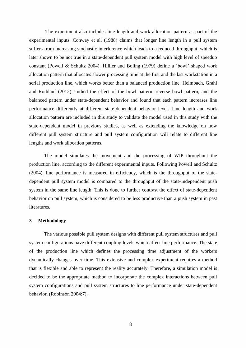
4.3 Simulation Model Validation
The result of the simulation model is compared with the result of previous state-
dependent model by Powell and Schultz (2004), which is used as the foundation for the
current state-dependent model.
Figure 4.2 Efficiency On Different Speedup Constants
The result produced by the model has similar interaction between speedup constant
and line performance with the result produced by the past model (figure 4.2), even though the
model used in this study has a slightly higher efficiency. This higher performance is caused by
a different mechanism of processing time adjustment. Powell and Schultz (2004) modeled the
processing time adjustment based on Markov models, while the current study adapted the
mathematical model proposed by Heimbach, Grahl and Rothlauf (2012). Adjusting processing
time based on the different state of the system is less sensitive compared to a mathematical
model that continuously adjusts according to the slightest changes in the system.
0.7
0.8
0.9
1
1.1
1.2
1.3
1.4
0 0.1 0.2 0.3 0.4 0.5 0.6 0.7 0.8 0.9 1
Effi
cie
ncy
Speed up constant (f)
Powell & Schultz (2004)
Current model

16
4.4 Simulation Result
The explanation of each simulation result in this section is done according to each of
the experimental variables. The impact of pull system structures and pull system
configurations to line performance under state-dependent behavior will be outlined
afterwards, followed by the work allocations and line lengths. Most of the results shown to
study the impact are taken from 3 workstations instead of 5 workstations to simplify and give
a clearer view of the effect. The complete summary of the simulation result can be found in
Appendix D.
4.4.1 Structure, Configuration, and Speedup Constant
Figure 4.3 Efficiency of each structure on increasing configuration
It can be observed in figure 4.3 that the increase in configuration also increases the
line performance, with a diminishing rate of increase. The slope of the graph shows that lower
configuration induces higher increase in line performance, compared to the higher
configuration. The effect on production performance resulting from the increase of the
speedup constant differs among structures. This different increase rate shows that line
performance of a pull system structure might reach an optimal level at higher pull system
configurations.
To understand how different structures affect line performance, the 3 different
structures are compared. However, it is not fair to directly compare the line performance of
the different pull system structures at the same configuration level. In 3 workstations settings,
0.20
0.40
0.60
0.80
1.00
1.20
1.40
1.60
0 1 2 3 4 5 6 7 8 910
Effi
cie
ncy
Configuration
CONWIP
0.20
0.40
0.60
0.80
1.00
1.20
1.40
1.60
0 1 2 3 4 5 6 7 8 910
Effi
cie
ncy
Configuration
POLCA
0.20
0.40
0.60
0.80
1.00
1.20
1.40
1.60
0 1 2 3 4 5 6 7 8 910
Effi
cie
ncy
Configuration
Kanban

17
a configuration of 5 in CONWIP structure with 1 control loop has the maximum WIP of 5.
POLCA structure with the same configuration level allows a maximum of 10 WIP, because
there are 2 control loops that are assigned with configuration of 5 in each of the control loops.
A Kanban structure that has 3 control loops has a maximum of 15 WIP in the production line.
In order to make an equal comparison, a level of 6 maximum WIP is used. The line
performance of the Kanban structure outperforms CONWIP and POLCA (table 4.3). The gap
of the line performance between the different structures gets wider as the effect of state-
dependent behavior gets stronger.
Speedup constant
CONWIP
(Configuration = 6,
Max WIP = 6)
POLCA
(Configuration = 3,
Max WIP = 6)
Kanban
(Configuration = 2,
Max WIP = 6)
0.1 0.80 0.72 0.85
0.5 0.94 0.83 1.04
1 1.12 1.03 1.33 Table 4.3 Efficiency of different structures under the same maximum WIP
In figure 4.4, it can be concluded that Kanban structure has more benefit from state-
dependent behavior compared to the POLCA and CONWIP pull system structures. However,
POLCA structure which is considered to have a tighter coupling than CONWIP has the lowest
performance. This shows that coupling in a pull system is not defined by the number of
control loops alone. The position of the control loops over the entire pull system structure also
affects the dynamic of the WIP, which critically affect the result.

18
4.4.2 Structure, Configuration, and Work Allocation
Figure 4.4 Production line efficiency under different work allocation pattern
0.20
0.40
0.60
0.80
1.00
1.20
0 1 2 3 4 5 6 7 8 910
Effi
cie
ncy
Configuration
CONWIP f=0.1
0.20
0.40
0.60
0.80
1.00
1.20
1.40
0 1 2 3 4 5 6 7 8 910
Effi
cie
ncy
Configuration
CONWIP f=0.5
0.20
0.40
0.60
0.80
1.00
1.20
1.40
1.60
1.80
0 1 2 3 4 5 6 7 8 910
Effi
cie
ncy
Configuration
CONWIP f=1
0.20
0.40
0.60
0.80
1.00
1.20
0 1 2 3 4 5 6 7 8 910
Effi
cie
ncy
Configuration
POLCA f=0.1
0.20
0.40
0.60
0.80
1.00
1.20
1.40
0 1 2 3 4 5 6 7 8 910
Effi
cie
ncy
Configuration
POLCA f=0.5
0.20
0.40
0.60
0.80
1.00
1.20
1.40
1.60
1.80
0 1 2 3 4 5 6 7 8 910
Effi
cie
ncy
Configuration
POLCA f=1
0.20
0.40
0.60
0.80
1.00
1.20
0 1 2 3 4 5 6 7 8 910
Effi
cie
ncy
Configuration
Kanban f=0.1
0.20
0.40
0.60
0.80
1.00
1.20
1.40
0 1 2 3 4 5 6 7 8 910
Effi
cie
ncy
Configuration
Kanban f=0.5
0.20
0.40
0.60
0.80
1.00
1.20
1.40
1.60
1.80
0 1 2 3 4 5 6 7 8 910
Effi
cie
ncy
Configuration
Kanban f=1

19
According to figure 4.5, the line performance of different structures tends to behave
similarly under the influence of state-dependent behavior. Under low speedup constant,
balanced pattern works better than bowl and reverse bowl pattern. But, the production
performance of reverse bowl pattern slowly outperforms the bowl pattern along the increase
of speedup effect, and finally tops the other patterns on the highest speedup constant.
Similar results are also shown by Heimbach, Grahl and Rothlauf (2012) in comparing
the best work allocation pattern with different speedup constant on low configuration settings.
On low and moderate speedup constant, the bowl shaped work allocation pattern and the
balanced line works best. As the speedup constant increases, reverse bowl work allocation
pattern becomes the best.
Work
Allocation
Pattern
Speedup
Constant
CONWIP
(Configuration = 6,
Max WIP = 6)
POLCA
(Configuration = 3,
Max WIP = 6)
Kanban
(Configuration = 2,
Max WIP = 6)
Reverse
Bowl
0.1 0.69 0.63 0.71
0.5 0.91 0.73 0.95
1 1.16 0.91 1.32
Bowl
0.1 0.72 0.69 0.79
0.5 0.86 0.84 0.95
1 1.05 1.06 1.24 Table 4.4 Efficiency of different structures under the same maximum WIP
Similarly with the result in a balanced work allocation pattern, Kanban is still the best
pull system structure in different work allocation patterns, while CONWIP is the second best,
and POLCA as the last. This shows that work allocation pattern does not respond differently
to Kanban, POLCA, and CONWIP structures.

20
4.4.3 Structure, Configuration, and Line Length
Figure 4.5 Efficiency on Different Line Lengths
0.00
0.20
0.40
0.60
0.80
1.00
1.20
1.40
0 1 2 3 4 5 6 7 8 910
Effi
cie
ncy
Configuration
CONWIP f = 0.1
0.00
0.20
0.40
0.60
0.80
1.00
1.20
1.40
0 1 2 3 4 5 6 7 8 910
Effi
cie
ncy
Configuration
CONWIP f = 0.5
0.00
0.20
0.40
0.60
0.80
1.00
1.20
1.40
0 1 2 3 4 5 6 7 8 910
Effi
cie
ncy
Configuration
CONWIP f = 1
0.00
0.20
0.40
0.60
0.80
1.00
1.20
1.40
1.60
0 1 2 3 4 5 6 7 8 910
Effi
cie
ncy
Configuration
POLCA f = 0.1
0.00
0.20
0.40
0.60
0.80
1.00
1.20
1.40
1.60
0 1 2 3 4 5 6 7 8 910
Effi
cie
ncy
Configuration
POLCA f = 0.5
0.00
0.20
0.40
0.60
0.80
1.00
1.20
1.40
1.60
0 1 2 3 4 5 6 7 8 910
Effi
cie
ncy
Configuration
POLCA f = 1
0.00
0.20
0.40
0.60
0.80
1.00
1.20
1.40
1.60
1.80
0 1 2 3 4 5 6 7 8 910
Effi
cie
ncy
Configuration
Kanban f = 0.1
0.00
0.20
0.40
0.60
0.80
1.00
1.20
1.40
1.60
1.80
0 1 2 3 4 5 6 7 8 910
Effi
cie
ncy
Configuration
Kanban f = 0.5
0.00
0.20
0.40
0.60
0.80
1.00
1.20
1.40
1.60
1.80
0 1 2 3 4 5 6 7 8 910
Effi
cie
ncy
Configuration
Kanban f = 1

21
The study by Heimbach, Grahl, and Rothlauf (2012) show that the deterioration of the
production performance is buffered by the state-dependent effect, while Powell and Schultz
(2004) show that a longer line will increase production performance under a high degree of
speedup effect. A similar result is obtained from this study, as can be seen in the graphs figure
4.6. Increasing the effect of the state-dependent behavior increased the line performance and
reduced the loss of line performance.
The result also shows that line performance of the Kanban structure in the high
speedup constant decreases in higher configuration. A similar result is also addressed by
Heimbach, Grahl and Rothlauf (2012) when increasing buffer capacity together with line
length. Allowing more WIP into the system increases throughput, but also allows more
variability and decreases the effect from state-dependent behavior. This makes the line
performance to be decreased after reaching an optimal performance in a certain pull system
configuration.
22
5 Discussion
The results demonstrated above reveal that difference in pull system structure and pull
system configuration play a role in affecting line performance. Still, the experimental design
used in this study only shows a limited view on the effect. In this section, further analysis is
done on the effect of pull system structure and pull system configuration on line performance,
and their implications on other pull system designs.
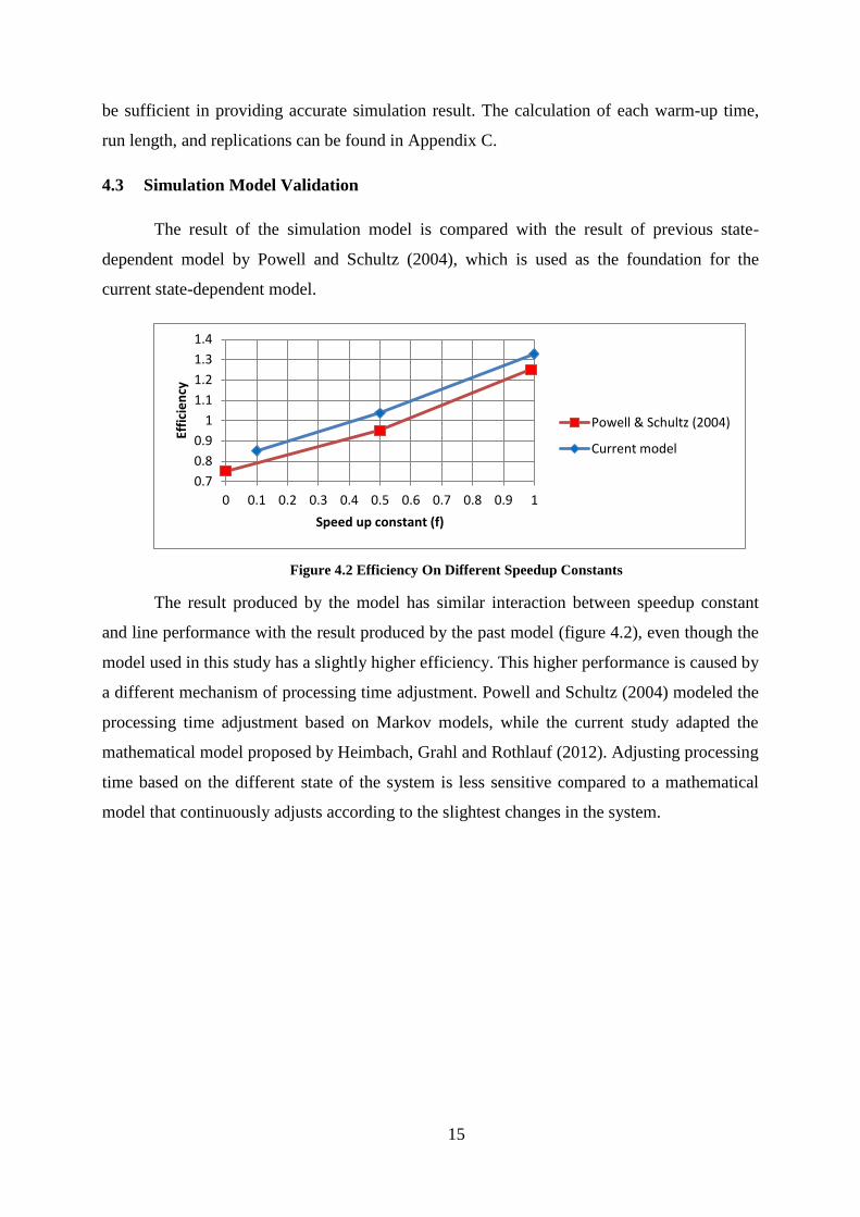
5.1 Pull System Configuration
The diminishing rate of line performance increase from increasing the configuration
level indicates that there might be an optimal performance level. The different rate of increase
also shows that a possibility of a certain structure might outperform the other at a higher
configuration level. To address this issue, an additional simulation in the higher configuration
for each pull system structure is done.
Figure 5.1 Efficiency on excessively higher pull system configurations
In higher configuration levels, line performance of the different pull system structures
seems to reach a certain level that is close to equal (figure 5.1). This shows that flooding the
pull system with WIP will lead to the different pull system structures to behave similarly. This
is explained by the formula used to model the processing time adjustment (Equation 1).
Assuming that the maximum capacity of each buffer used as the benchmark to adjust
processing time is the pull system configuration, putting a large number as the capacity will
1.20
1.25
1.30
1.35
1.40
1.45
1.50
1.55
1.60
0 10 20 30 40 50 60 70 80 90100
Effi
cie
ncy
Configuration
3 Workstations
0.00
0.20
0.40
0.60
0.80
1.00
1.20
1.40
1.60
0 10 20 30 40 50
Effi
cie
ncy
Configuration
5 Workstations
23
bring the average processing time of the system to almost half of the initial average processing
time. The first station will work half of the average initial processing time since the large
capacity makes the model treat the downstream buffer as empty and has to be filled. On the
other hand, the last station will work at the normal processing time because the large capacity
leads to the model behave as if there is only a very small number of WIP queuing in the
buffer. Meanwhile, the middle workstations are having a combined effect of the previous two
assumptions.
The result of the 5 workstations shows a decreasing line performance, which does not
happen to the 3 workstations setting. This happens due to the high variation in longer line
length (Conway et al. 1988). The high variation interferes the performance of the line, and
nullifies the positive effect of the state-dependent behavior.
In reality, increasing the buffer capacity of the pull system excessively would
transform the pull system into a push system. Workers that are initially aware of the buffer
state will cease to be concerned with the state of the buffer when the buffer limit is too high to
be noticeable, and return to their initial average processing time. The model used in this study
has not yet facilitated the diminishing effect of state-dependent behavior that occurs when
buffer capacity increases. To be able to create a more accurate processing time adjustment
model, empirical data would be needed.
5.2 Pull System Structure
To see the role of the pull system structure, the workstations and the buffers being
regulated by the structure have to be examined individually. In figure 5.2, the average
processing times of each workstation are displayed together with the average WIP level of
each buffer. The axis on the left of the chart shows the processing time unit, while the axis on
the right shows the average unit of WIP level in the buffer. The result of CONWIP, POLCA,
and Kanban pull system structures are compared assuming a balanced initial average
processing time and equal number of maximum WIP. The comparison is done in the context
of the highest state-dependent behavior effect to have a distinct effect.

24
Figure 5.2 Average Processing Times and Average WIP of CONWIP, POLCA, and Kanban in
Balanced Work Allocation
The smaller the area of a control loop, the more sensitive it gets to processing time
variability. Under state-dependent behavior, this occurrence increases the frequency of
processing time adjustment which minimizes processing time variability (Powell and Schultz,
2004). This effect is emphasized in the CONWIP and the POLCA which have less control
loops in their structure. The CONWIP structure does not strictly limit the middle workstation,
while the POLCA structure limits it through control from the beginning of the first
workstation. This difference in structure creates a higher processing time of the middle
workstation in CONWIP and POLCA structure, because of the unadjusted variability in
processing times.
Powell and Schultz (2004) mentioned in their study in a single Kanban structure
production line, that the middle workstation would have the most speedup effect of state-
dependent behavior since it is affected by both the upstream and downstream buffer. The
exact result is obtained from the Kanban structure in this study, while other pull system
structures have different processing time distribution. This makes it reasonable to implement a
certain work allocation pattern according to the average processing time distribution, which is
a reversed bowl pattern in the case of Kanban pull system structure.
Aside for processing time distribution, different pull system structures have different
WIP level distribution among the buffers. The simulation results show that POLCA has the
lowest performance, however, it also has the lowest average and most balanced WIP level in
each buffer compared to the other structures. This fact may not be interesting in the case that
0.00
0.50
1.00
1.50
2.00
2.50
0.000.200.400.600.801.001.201.401.601.802.002.202.40
Avg. processingtime
workstation 1
Avg. WIP inBuffer 1
Avg. processingtime
workstation 2
Avg. WIP inBuffer 2
Avg. processingtime
workstation 3
Ave
rage
WIP
in B
uff
er
Pro
cess
ing
tim
e
CONWIP Processing Time POLCA Processing Time Kanban Processing Time
CONWIP Buffer POLCA Buffer Kanban Buffer

25
only throughput is considered as the performance measure. But, WIP is an important measure
for a pull system because preventing WIP explosion and reducing WIP level is one of the
most important features of pull system (Hopp & Spearman 2004).
5.3 Work In Process
It is difficult to monitor the average WIP directly from the simulation model.
However, the average WIP of the simulation model can be obtained through Little’s law
(Hopp and Spearman 2008:239) with the formula:
This method of calculating average WIP is less accurate than direct measurement
because of the variation in throughput and cycle time. Throughput in this calculation is the
average output per unit time, while cycle time is the average time from when a job is released
into the station until it exits (Hopp and Spearman 2008:239). In this model, the cycle time is
calculated after a work enters the pull system structure and becomes a WIP.
Speedup constant
CONWIP
(Configuration = 6,
Max WIP = 6)
POLCA
(Configuration = 3,
Max WIP = 6)
Kanban
(Configuration = 2,
Max WIP = 6)
0.1 5.98 4.21 6.13
0.5 6.05 4.37 6.55
1 6.00 4.77 6.89
Table 5.1 Average WIP With Equal Level Of Maximum WIP
Table 5.1 shows the POLCA structure has the lowest average WIP, while CONWIP
and Kanban structures used the maximum WIP on average. This means that the Kanban and
CONWIP structures are blocked at most of the time during the process but still manage to
perform efficiently. The fact that Kanban has slightly higher WIP also contradicts with the
earlier finding by Khojasteh-Ghamari (2009) that claims Kanban has a better WIP
minimization ability in a balanced work allocation pattern in state-independent settings.
The result above is in line with the performance of each structure where higher WIP
supports line performance. However, this relation between WIP and throughput has different
strength between different structures. To understand the relation, the efficiency of the line is
divided by the average WIP.

26
Speedup constant
CONWIP
(Configuration = 6,
Max WIP = 6)
POLCA
(Configuration = 3,
Max WIP = 6)
Kanban
(Configuration = 2,
Max WIP = 6)
0.1 0.134 0.171 0.139
0.5 0.155 0.190 0.159
1 0.187 0.216 0.193 Table 5.2 Production Line Efficiency Relative to Their Average WIP
From the result in table 5.2, POLCA has the highest throughput efficiency over
average WIP compared to Kanban and CONWIP. It can be said that POLCA is the best
structure to use WIP efficiently to produce throughput under state-dependent behavior.
This is a discovery from one out of hundred different possible pull system structures.
Through the generic structure proposed by Gaury, Kleijnen and Pierreval (2001), further
research on different pull system structures and configurations under state-dependent behavior
can discover other optimal pull system designs.
6 Conclusion
Through the simulation, analysis, and discussions the objective of the research has
been achieved. This study has done its intended contribution, although still limited. These
limitations are considered as an insight for future research in state-dependent behavior.
6.1 Conclusion
Aiming to provide a better understanding of pull system design under the influence of
state-dependent behavior, this study has been done to answer the initial research question:
What is the impact of pull system structure and configuration on line performance given state-
dependent behavior? There are two main findings that answer the research question directly.
The pull system structure with tighter coupling effect has more benefit of increasing
line performance compared to other pull system structure with less coupling. However, tighter
coupling means more sensitivity to variation, which means that it is more prone to line
performance decrease in longer line length.
Meanwhile, increasing pull system configuration increases line performance with a
diminishing rate of increase, until it reached a certain level of where maximum processing
time adjustment occurs. This performance may decrease in longer line length, due to higher
variations.

27
Aside from pull system structure and pull system configuration, this study also
discovered several side findings on other aspects of pull system design. These side findings
provide further explanation on the main research question and complement the study.
Pull system structure under state-dependent behavior has a self-balancing mechanism
(Powell & Schultz 2004), but also alters the initially balanced work allocation pattern into an
imbalanced allocation pattern. Allocating higher workload to workstations with faster work
processing time, and lower workload to the workstations with slower processing time, will
result in higher line performance.
In extended production lines, the decrease of line performance is minimized under
state-dependent behavior due to more interior workers that have faster processing times. Pull
system structures with tighter coupling are more prone to experience line performance
decrease on longer line length, because of the higher sensitivity to workflow disturbance from
variations.
Analyzing the average WIP shows that different pull system structures have different
performance in minimizing WIP under state-dependent behavior. The POLCA structure has
the highest line performance-to-average WIP ratio compared to other pull system structures,
showing that it has better capability to minimize WIP usage while efficiently processing it
into finished goods.
6.2 Recommendations
The Kanban pull system structure provides the best performance under state-
dependent behavior. On the other hand, the POLCA pull system structure is one example that
provides both sufficiently high throughput compared to the push system, and low average
WIP level.
It is more feasible for management to manipulate pull system structure and
configuration compared to manipulate the length of the line or work allocation in order to
achieve higher performance. Pull system structure and pull system configuration has the
capability to distribute workload. By designing the pull system to distribute a higher workload
to faster workstations, and lower workload to slower workstation, will result in higher
performance.

28
Pull system design for longer line length has to consider their stochastic nature.
Implementing a pull system structure with tighter coupling to small parts of the production
system rather than to the entire production line might be more beneficial.
6.3 Limitations and suggestions for future research
Cost efficiency can be used instead of throughput to measure line performance, which
is able to incorporate important aspects of a production system. Designing a cost effective pull
system does not only focus in the capability to provide a high throughput. The capability of a
pull system to minimize WIP is an important part that has to be paid attention to minimize
operating expense.
From thousands of different possible pull system structure, only three structures are
studied. These possible structures might be able to provide more cost efficient pull system
design than the Kanban, POLCA, and CONWIP pull system structures. On the other hand,
non-identical configuration between control loops should also be considered in future research
to accommodate workload distribution with varying intensity. To perform a study with a vast
search space, a heuristic method is needed to perform the simulation effectively. Evolutionary
algorithm that is used in the study by Gaury, Kleijnen and Pierreval (2001) is an example of a
heuristic method with the capability to efficiently search the optimal result.
The state-dependent behavior model that is used to adjust workers’ processing time
has not completely incorporates the propensity of decreasing state-dependent behavior effect
on higher buffer capacity. Increasing the buffer capacity of a pull system would
disproportionately reduce or even erase the state-dependent behavior effect, and alters the pull
system into a state-independent push system. This further development of the model has be
based on concrete empirical research in a real production system.
The pull system model should facilitate stochastic inter-arrival times. In most
industries, order does not come at a constant rate, and this increases the variations in the
system even further. The processing time of each workstation should be distributed with a
Coefficient of Variation (CV) around 0.35, to represent the actual variations of a human
worker based on an empirical study (Schultz et al. 1998).
Humans are not machines. Hence, each individual obviously reacts differently on the
situations around them. Therefore, state-dependent behavior model in future studies should
consider implementing different speedup constant on each individual worker.

29
References
1. Conway, R., Maxwell, W., McClain, J. and Thomas, L. (1988). “The Role of Work-in-
Process Inventory in Serial Production Lines”. Operations Research, 36(2), pp.229-
241.
2. Doerr, K., Mitchell, T., Klastorin, T. and Brown, K. (1996). “Impact of material flow
policies and goals on job outcomes”. Journal of Applied Psychology, 81(2), pp.142-
152.
3. Edie, L. (1954). “Traffic Delays at Toll Booths”. OR, 2(2), pp.107-138.
4. Franks, I. and Sury, R. (1966). “The performance of operators in conveyor-paced
work”. International journal of production research, 5(2), pp.97-112.
5. Gaury, E., Kleijnen, J. and Pierreval, H. (2001). “A methodology to customize pull
control systems”. Journal of the Operational Research Society, 52(7), pp.789-799.
6. Gaury, E., Pierreval, H. and Kleijnen, J. (2000). “Evolutionary approach to select a
pull system among Kanban, Conwip and Hybrid”. Journal of Intelligent
Manufacturing, 11, pp.157-167.
7. Germs, R. and Riezebos, J. (2010).” Workload balancing capability of pull systems in
MTO production”. International Journal of Production Research, 48(8), pp.2345-
2360.
8. Heidelberger, P. and Welch, P. (1983). “Simulation Run Length Control in the
Presence of an Initial Transient”. Operations Research, 31(6), pp.1109-1144.
9. Heimbach, I., Grahl, J. and Rothlauf, F. (2012). “The effects of state-dependent human
behavior on the design of a serial line”. Z Betriebswirtsch, 82(7-8), pp.745-762.
10. Hillier, F. and Boling, R. (1966). “The effect of some design factors on the efficiency
of production lines with variable operation times”. Journal of Industrial Engineering,
17, pp.651-658.
11. Hillier, F. and Boling, R. (1979). “On the Optimal Allocation of Work in
Symmetrically Unbalanced Production Line Systems with Variable Operation Times”.
Management Science, 25(8), pp.721-728.
12. Hopp, W. and Spearman, M. (2004). To Pull or Not to Pull: “What Is the Question?”.
Manufacturing & Service Operations Management, 6(2), pp.133-148.
13. Hopp, W. and Spearman, M. (2008). Factory physics. New York, NY: McGraw-
Hill/Irwin/Irwin.

30
14. Khojasteh-Ghamari, Y. (2009). “Developing a framework for performance analysis of
a production process controlled by Kanban and CONWIP”. Journal of Intelligent
Manufacturing, 23(1), pp.61-71.
15. Krishnamurthy, A. and Suri, R. (2009).”Planning and implementing POLCA: a card-
based control system for high variety or custom engineered products”. Production
Planning & Control, 20(7), pp.596-610.
16. Müller, K.., Vignaux, T., (2010). SimPy (Version 3.0.6) [Computer program].
Available: http://simpy.sourceforge.net/ (Acessed 5 February 2015)
17. Powell, S. and Schultz, K. (2004). “Throughput in Serial Lines with State-Dependent
Behavior”. Management Science, 50(8), pp.1095-1105.
18. Robinson, S. (1995). “A Heuristic Technique for Selecting the Run-Length of Non-
Terminating Steady-State Simulations”. SIMULATION, 65(3), pp.170-179.
19. Robinson, S. (2004). Simulation. Chichester, Eng.: Wiley.
20. Schultz, K., Juran, D., Boudreau, J., McClain, J. and Thomas, L. (1998). “Modeling
and Worker Motivation in JIT Production Systems”. Management Science, 44(12-part-
1), pp.1595-1607.
21. Schultz, K., Juran, D. and Boudreau, J. (1999). “The Effects of Low Inventory on the
Development of Productivity Norms. Management Science, 45(12), pp.1664-1678.
22. Shunko, M., Niederhoff, J. and Rosokha, Y. (2014). “Humans are Not Machines:
Impact of Queuing Design on Service Time”. [Online]. Available at SSRN:
http://ssrn.com/abstract=2479342
23. Spearman, M., Woodruff, D. and Hopp, W. (1990). “CONWIP: a pull alternative to
kanban”. Int. J. of Prodn. Res., 28(5), pp.879-894.
24. Sugimori, Y., Kusunoki, K., Cho, F. And Uchikawa, S. (1977). “Toyota production
system and Kanban system Materialization of just-in-time and respect-for-human
system”. International Journal of Production Research, 15(6), pp.553-564.
25. Tan, T. and Netessine, S. (2014). “When Does the Devil Make Work? An Empirical
Study of the Impact of Workload on Worker Productivity”. Management Science,
60(6), pp.1574-1593.
26. Van Rossum, G. (1995). Python reference manual. Amsterdam, the Netherlands:
Centrum voor Wiskunde en Informatica.
27. Ziengs, N., Riezebos, J. and Germs, R. (2012). “Placement of effective work-in-
progress limits in route-specific unit-based pull systems”. International Journal of
Production Research, 50(16), pp.4358-4371.

31
APPENDIX A: WIP Movement Flowchart
The movement of the WIP in the simulation model is coded into the simulation
software according to the following flowchart. Pull system structures and pull system
configurations affect the WIP movement through the number of cards in every stage of the
movement.
Start
WIP
Any card required to move to the next workstation ?
Wait for the required card to be available
YESIs the required card available ?
YES
NO
NO
Wait in the buffer until workstation ahead becomes available
NO Is the workstation ahead available ?
YES
Move to workstation ahead and Start processing according to the
processing time adjustment model
YES
Is this the last workstation in the line ?
Any attached card that has to be released ?
Release cardYES
EndBlock the current machine until the
next buffer is availavle
NO
Is the next buffer available?
Move to the next buffer
YES
Attach the required card
NO
Figure.Appendix 1 WIP Movement Flowchart

32
APPENDIX B: Workers processing time adjustment model
The processing times of each workstation in the simulation model is coded according
to the following flowchart. Initially, the WIP is processed according to the initial state of the
buffer before the processing starts. During the process, the state of the buffer is continuously
monitored, and adjustment is made to the remaining processing time for every change of WIP
level in the upstream or downstream buffer.
Start
Mean processing times
Is the downstream buffer in full capacity?
YES(C-ci,i+1) = 0
NO
Is the upstream buffer empty?(ci-1,i)/C = 0 YES
NO
Process inventory according to the following formula:wi
adj =wi – f * (wi /2) * ((ci-1,i)/C)- f * (wi /2) * ((C-ci,i+1)/C)
Is there a new WIP entering the upstream buffer ?
YESAdjust remaining processing time into
wi+1rem,adj =wi+1
rem -f * (1/C)*wi+1rem
NO
Is there a WIP leaving the downstream buffer ?
NO
Adjust remaining processing time into wi
rem,adj =wirem -f * (1/C)*wi
rem
NO
EndHas the workstation finished
processing?
YES
YES
Figure.Appendix 2 Processing time adjustment flowchart
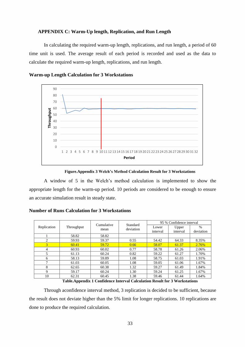
33
APPENDIX C: Warm-Up length, Replication, and Run Length
In calculating the required warm-up length, replications, and run length, a period of 60
time unit is used. The average result of each period is recorded and used as the data to
calculate the required warm-up length, replications, and run length.
Warm-up Length Calculation for 3 Workstations
Figure.Appendix 3 Welch’s Method Calculation Result for 3 Workstations
A window of 5 in the Welch’s method calculation is implemented to show the
appropriate length for the warm-up period. 10 periods are considered to be enough to ensure
an accurate simulation result in steady state.
Number of Runs Calculation for 3 Workstations
Replication Throughput Cumulative
mean
Standard
deviation
95 % Confidence interval
Lower
interval
Upper
interval
%
deviation
1 58.82 58.82
2 59.93 59.37 0.55 54.42 64.33 8.35%
3 60.41 59.72 0.66 58.07 61.37 2.76%
4 60.93 60.02 0.77 58.78 61.26 2.06%
5 61.13 60.24 0.82 59.22 61.27 1.70%
6 58.13 59.89 1.08 58.75 61.03 1.91%
7 61.03 60.05 1.08 59.05 61.06 1.67%
8 62.65 60.38 1.32 59.27 61.49 1.84%
9 59.17 60.24 1.30 59.24 61.25 1.67%
10 62.31 60.45 1.38 59.46 61.44 1.64%
Table.Appendix 1 Confidence Interval Calculation Result for 3 Workstations
Through aconfidence interval method, 3 replication is decided to be sufficient, because
the result does not deviate higher than the 5% limit for longer replications. 10 replications are
done to produce the required calculation.
0
10
20
30
40
50
60
70
80
90
1 2 3 4 5 6 7 8 9 10 11 12 13 14 15 16 17 18 19 20 21 22 23 24 25 26 27 28 29 30 31 32
Thro
ugh
pu
t
Period

34
Run Length Calculation for 3 Workstations
Replication 1 Replication 2 Replication 3
Period Result Cum.mean
average Result
Cum.mean
average Result
Cum.mean
average Convergence
1 49 49 92 92 94 94 91.84%
2 56 52.50 52 58.42 62 65.69 25.13%
3 63 56.00 66 59.50 56 63.83 13.98%
4 60 57.00 66 59.88 50 62.51 9.67%
5 66 58.80 44 59.15 60 61.53 4.64%
6 57 58.50 54 58.71 56 60.75 3.84%
7 63 59.14 61 59.04 74 61.10 3.49%
8 61 59.38 52 58.85 56 60.65 3.06%
9 55 58.89 63 58.86 57 60.41 2.64%
10 48 57.80 63 58.60 66 60.24 4.22%
11 64 58.36 52 58.56 51 59.93 2.68%
12 48 57.50 57 58.19 60 59.61 3.67%
13 59 57.62 64 58.35 80 59.93 4.02%
14 49 57.00 44 57.75 50 59.33 4.09%
15 81 58.60 61 58.36 67 59.72 2.34%
16 56 58.44 65 58.45 59 59.70 2.16%
17 58 58.41 53 58.33 61 59.59 2.15%
18 64 58.72 57 58.42 59 59.58 1.98%
19 55 58.53 66 58.49 70 59.69 2.04%
20 59 58.55 58 58.50 62 59.66 1.99%
Table.Appendix 2 Run Length Graphical Method Calculation Result for 3 Workstations
Figure.Appendix 4 Run Length Graphical Method Calculation Graph for 3 Workstations
In the graphical method, convergence level less than 3% is chosen instead of 5% to
ensure accuracy of the data. 15 periods or 900 units of time are considered sufficient since the
convergence level remains at the same even for a longer time period.
40
50
60
70
80
90
100
1 3 5 7 9 11 13 15 17 19 21 23 25 27 29
Thro
ugh
pu
t
Period
Replication 1
Replication 2
Replication 3

35
Warm-up Length Calculation for 5 Workstations
Figure.Appendix 5 Welch’s Method Calculation Result for 5 Workstations
Using the same number for window to calculate the length of the warm-up period for
the 5 workstation setting, 10 periods of time are considered stable to provide an accurate
simulation result.
Number of Runs Calculation for 5 Workstations
Replication Mean time in system
Cumulative mean
Standard deviation
95 % Confidence interval
Lower interval
Upper interval
% deviation
1 59.97 59.97
2 60.20 60.08 0.11 59.05 61.12 1.73%
3 57.12 59.10 1.39 55.62 62.57 5.88%
4 58.44 58.93 1.24 56.95 60.91 3.36%
5 59.61 59.07 1.14 57.65 60.49 2.41%
6 58.97 59.05 1.04 57.95 60.15 1.86%
7 60.07 59.20 1.03 58.24 60.15 1.61%
8 60.20 59.32 1.02 58.47 60.18 1.44%
9 59.23 59.31 0.96 58.57 60.05 1.25%
10 61.66 59.55 1.15 58.72 60.37 1.39%
Table.Appendix 3 Confidence Interval Calculation Result for 5 Workstations
Based on this calculation, 4 replications are needed to provide accurate results in
simulation with 5 workstation setting. It is decided to implement 4 replications for both the 3
and 5 workstations, assuming that more replications will provide a more accurate data.
0
10
20
30
40
50
60
70
80
1 4 7 10 13 16 19 22 25 28 31 34 37 40 43 46 49 52 55 58
Fin
ish
ed
Pro
du
cts
Period

36
Run Length Calculation for 5 Workstations
Replication 1 Replication 2 Replication 3
Period Result Cum.mean
average Result
Cum.mean
average Result
Cum.mean
average Convergence
1 60 60 85 85 86 86 43.33%
2 60 60 56 63.5 57 67.25 12.08%
3 67 62.33 44 61.59 59 64.42 4.60%
4 54 60.25 45 59.46 49 61.70 3.77%
5 55 59.2 57 58.98 59 60.93 3.30%
6 60 59.33 56 58.89 56 60.45 2.64%
7 53 58.42 63 58.78 57 60.10 2.87%
8 59 58.5 62 58.91 61 60.07 2.70%
9 67 59.44 57 59.16 67 60.28 1.89%
10 51 58.6 63 59.002 56 60.008 2.40%
11 63 59 47 58.76 60 59.78 1.74%
12 61 59.16 62 58.92 60 59.82 1.52%
13 73 60.23 63 59.42 54 59.98 1.36%
14 71 61 52 59.55 45 59.82 2.42%
15 70 61.6 60 59.84 47 59.81 2.99%
16 65 61.81 70 60.20 70 60.16 2.74%
17 50 61.11 60 60.01 74 60.21 1.83%
18 52 60.611 67 60.01 66 60.26 1.00%
19 69 61.052 63 60.24 47 60.25 1.35%
20 63 61.15 57 60.24 45 60.103 1.74%
20 63 61.15 57 60.24 45 60.1 1.74%
21 65 61.33 78 60.62 53 60.26 1.76%
22 55 61.04 62 60.56 64 60.28 1.27%
23 55 60.78 53 60.37 54 60.12 1.10%
24 64 60.91 70 60.56 44 60.11 1.34%
25 61 60.92 67 60.66 56 60.15 1.27%
20 63 61.15 57 60.24 45 60.103 1.74%
21 65 61.33 78 60.62 53 60.26 1.76%
22 55 61.04 62 60.56 64 60.28 1.27%
23 55 60.78 53 60.37 54 60.12 1.10%
24 64 60.91 70 60.56 44 60.11 1.34%
25 61 60.92 67 60.66 56 60.15 1.27%
26 49 60.46 60 60.50 64 60.101 0.67%
27 64 60.59 46 60.36 57 60.008 0.97%
Table.Appendix 4 Run Length Graphical Method Calculation Result for 5 Workstations
Figure.Appendix 6 Run Length Graphical Method Graph for 5 Workstations
Convergence level less than 3% is achieved after 6 periods of run, but it does not have
stable results until 15 periods of run. Therefore, the longer period is considered sufficient
since the convergence level remains stable even for a longer time period.
55
60
65
70
75
80
85
90
1 3 5 7 9 11 13 15 17 19 21 23 25 27 29 31
Thro
ugh
pu
t
Period
Replication 1
Replication 2
Replication 3
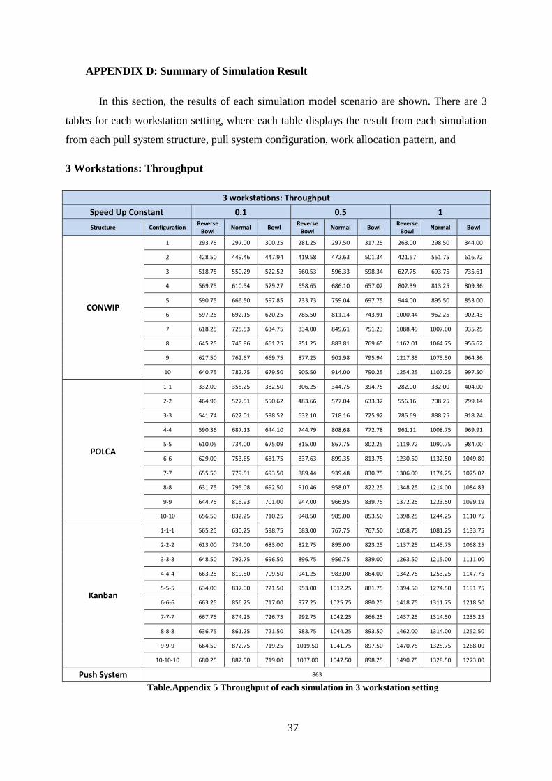
37
APPENDIX D: Summary of Simulation Result
In this section, the results of each simulation model scenario are shown. There are 3
tables for each workstation setting, where each table displays the result from each simulation
from each pull system structure, pull system configuration, work allocation pattern, and
3 Workstations: Throughput
3 workstations: Throughput
Speed Up Constant 0.1 0.5 1
Structure Configuration Reverse
Bowl Normal Bowl
Reverse Bowl
Normal Bowl Reverse
Bowl Normal Bowl
CONWIP
1 293.75 297.00 300.25 281.25 297.50 317.25 263.00 298.50 344.00
2 428.50 449.46 447.94 419.58 472.63 501.34 421.57 551.75 616.72
3 518.75 550.29 522.52 560.53 596.33 598.34 627.75 693.75 735.61
4 569.75 610.54 579.27 658.65 686.10 657.02 802.39 813.25 809.36
5 590.75 666.50 597.85 733.73 759.04 697.75 944.00 895.50 853.00
6 597.25 692.15 620.25 785.50 811.14 743.91 1000.44 962.25 902.43
7 618.25 725.53 634.75 834.00 849.61 751.23 1088.49 1007.00 935.25
8 645.25 745.86 661.25 851.25 883.81 769.65 1162.01 1064.75 956.62
9 627.50 762.67 669.75 877.25 901.98 795.94 1217.35 1075.50 964.36
10 640.75 782.75 679.50 905.50 914.00 790.25 1254.25 1107.25 997.50
POLCA
1-1 332.00 355.25 382.50 306.25 344.75 394.75 282.00 332.00 404.00
2-2 464.96 527.51 550.62 483.66 577.04 633.32 556.16 708.25 799.14
3-3 541.74 622.01 598.52 632.10 718.16 725.92 785.69 888.25 918.24
4-4 590.36 687.13 644.10 744.79 808.68 772.78 961.11 1008.75 969.91
5-5 610.05 734.00 675.09 815.00 867.75 802.25 1119.72 1090.75 984.00
6-6 629.00 753.65 681.75 837.63 899.35 813.75 1230.50 1132.50 1049.80
7-7 655.50 779.51 693.50 889.44 939.48 830.75 1306.00 1174.25 1075.02
8-8 631.75 795.08 692.50 910.46 958.07 822.25 1348.25 1214.00 1084.83
9-9 644.75 816.93 701.00 947.00 966.95 839.75 1372.25 1223.50 1099.19
10-10 656.50 832.25 710.25 948.50 985.00 853.50 1398.25 1244.25 1110.75
Kanban
1-1-1 565.25 630.25 598.75 683.00 767.75 767.50 1058.75 1081.25 1133.75
2-2-2 613.00 734.00 683.00 822.75 895.00 823.25 1137.25 1145.75 1068.25
3-3-3 648.50 792.75 696.50 896.75 956.75 839.00 1263.50 1215.00 1111.00
4-4-4 663.25 819.50 709.50 941.25 983.00 864.00 1342.75 1253.25 1147.75
5-5-5 634.00 837.00 721.50 953.00 1012.25 881.75 1394.50 1274.50 1191.75
6-6-6 663.25 856.25 717.00 977.25 1025.75 880.25 1418.75 1311.75 1218.50
7-7-7 667.75 874.25 726.75 992.75 1042.25 866.25 1437.25 1314.50 1235.25
8-8-8 636.75 861.25 721.50 983.75 1044.25 893.50 1462.00 1314.00 1252.50
9-9-9 664.50 872.75 719.25 1019.50 1041.75 897.50 1470.75 1325.75 1268.00
10-10-10 680.25 882.50 719.00 1037.00 1047.50 898.25 1490.75 1328.50 1273.00
Push System 863
Table.Appendix 5 Throughput of each simulation in 3 workstation setting

38
3 Workstations: Average Cycle Time
3 workstations: Average Cycle Time
speed up parameter 0.1 0.5 1
structure configuration reverse bowl normal bowl reverse bowl normal bowl reverse bowl normal bowl
CONWIP
1 3.06 3.04 3.00 3.20 3.03 2.84 3.43 3.01 2.62
2 4.22 4.01 4.05 4.36 3.91 3.63 4.36 3.26 3.04
3 5.22 4.91 5.21 4.87 4.60 4.53 4.34 3.90 3.76
4 6.33 5.89 6.24 5.50 5.32 5.51 4.51 4.43 4.49
5 7.64 6.76 7.54 6.15 6.01 6.46 4.77 5.03 5.28
6 9.08 7.78 8.73 6.88 6.71 7.32 5.46 5.61 6.08
7 10.20 8.68 9.94 7.55 7.43 8.45 5.84 6.26 6.81
8 11.17 9.65 10.92 8.46 8.16 9.38 6.23 6.77 7.60
9 12.98 10.61 12.12 9.25 8.99 10.21 6.68 7.53 8.44
10 14.06 11.51 13.33 9.97 9.88 11.42 7.19 8.16 9.05
POLCA
1-1 3.50 3.55 3.63 3.72 3.64 3.57 3.97 3.76 3.52
2-2 4.82 4.77 5.20 4.60 4.47 4.60 4.03 3.82 3.86
3-3 6.05 6.09 7.35 5.32 5.47 6.20 4.51 4.83 5.18
4-4 7.38 7.43 9.29 6.02 6.71 8.00 5.03 5.86 6.65
5-5 8.79 8.84 11.38 6.98 7.93 9.67 5.58 6.85 8.37
6-6 10.00 10.89 13.64 8.13 9.18 11.53 6.35 8.00 9.51
7-7 11.07 12.35 15.53 9.04 10.31 13.52 7.06 9.09 10.82
8-8 12.91 13.58 18.39 9.91 11.73 16.00 7.71 9.97 12.36
9-9 14.18 14.89 19.75 10.71 13.49 17.56 8.62 11.31 13.75
10-10 15.30 16.11 22.19 11.60 14.70 18.45 9.44 12.42 15.17
KANBAN
1-1-1 47.10 5.09 5.20 4.62 4.31 4.29 3.15 3.20 3.01
2-2-2 8.45 7.52 8.58 6.54 6.59 7.12 4.92 5.41 6.05
3-3-3 11.06 10.20 11.84 8.38 8.57 10.06 6.16 6.86 8.08
4-4-4 13.64 13.12 14.17 10.13 10.62 12.88 7.34 8.41 9.98
5-5-5 17.07 15.57 18.80 11.96 12.56 14.31 8.48 9.67 11.11
6-6-6 19.16 18.22 23.54 13.69 14.28 16.92 9.52 10.79 13.26
7-7-7 21.84 20.58 22.96 15.54 16.39 21.29 10.62 12.01 14.82
8-8-8 25.51 23.09 28.47 17.38 17.43 21.21 11.85 13.18 15.87
9-9-9 27.28 24.51 25.01 19.00 18.47 24.55 12.99 14.60 16.91
10-10-10 29.51 26.43 27.28 20.49 20.12 24.56 14.02 15.96 18.76
Table.Appendix 6 Average cycle time of each simulation in 3 workstation setting

39
3 Workstations: Average WIP
3 workstations: Average WIP
Speed Up Constant 0.1 0.5 1
Structure Configuration Reverse Bowl Normal Bowl Reverse Bowl Normal Bowl Reverse Bowl Normal Bowl
CONWIP
1 0.9988 1.0025 1.0009 1.0000 1.0003 1.0008 1.0012 0.9998 0.9997
2 2.0080 2.0032 2.0157 2.0344 2.0529 2.0237 2.0411 2.0000 2.0807
3 3.0067 2.9993 3.0222 3.0362 3.0451 3.0135 3.0253 3.0047 3.0721
4 4.0081 3.9963 4.0167 4.0242 4.0530 4.0193 4.0182 3.9997 4.0372
5 5.0159 5.0039 5.0059 5.0165 5.0651 5.0121 4.9988 5.0067 5.0017
6 6.0257 5.9840 6.0175 6.0058 6.0481 6.0532 6.0748 6.0033 6.0985
7 7.0044 6.9948 7.0104 6.9975 7.0103 7.0553 7.0671 6.9989 7.0719
8 8.0067 7.9963 8.0208 8.0034 8.0144 8.0191 8.0443 8.0044 8.0744
9 9.0494 8.9897 9.0200 9.0187 9.0138 9.0316 9.0394 8.9977 9.0441
10 10.0064 10.0120 10.0637 10.0316 10.0325 10.0262 10.0211 10.0356 10.0322
POLCA
1-1 1.2897 1.4029 1.5422 1.2644 1.3928 1.5678 1.2446 1.3887 1.5794
2-2 2.4910 2.7953 3.1793 2.4732 2.8684 3.2346 2.4911 3.0041 3.4291
3-3 3.6446 4.2088 4.8908 3.7394 4.3656 4.9970 3.9406 4.7676 5.2899
4-4 4.8402 5.6699 6.6462 4.9856 6.0300 6.8668 5.3711 6.5681 7.1662
5-5 5.9599 7.2078 8.5397 6.3180 7.6450 8.6190 6.9386 8.2984 9.1504
6-6 6.9862 9.1230 10.3347 7.5700 9.1780 10.4221 8.6793 10.0724 11.0910
7-7 8.0591 10.7001 11.9701 8.9324 10.7640 12.4795 10.2425 11.8555 12.9195
8-8 9.0652 11.9944 14.1488 10.0289 12.4876 14.6147 11.5530 13.4432 14.8989
9-9 10.1557 13.5196 15.3833 11.2736 14.4913 16.3873 13.1396 15.3696 16.7930
10-10 11.1640 14.8955 17.5135 12.2295 16.0877 17.4955 14.6609 17.1672 18.7283
Kanban
1-1-1 29.5828 3.5657 3.4585 3.5032 3.6779 3.6592 3.7063 3.8419 3.7966
2-2-2 5.7541 6.1299 6.5093 5.9782 6.5524 6.5120 6.2177 6.8880 7.1829
3-3-3 7.9690 8.9801 9.1593 8.3514 9.1076 9.3780 8.6448 9.2554 9.9777
4-4-4 10.0496 11.9487 11.1689 10.5916 11.6037 12.3673 10.9489 11.7112 12.7268
5-5-5 12.0271 14.4771 15.0689 12.6685 14.1295 14.0206 13.1448 13.6929 14.7090
6-6-6 14.1214 17.3366 18.7500 14.8662 16.2696 16.5510 15.0090 15.7322 17.9491
7-7-7 16.2017 19.9939 18.5419 17.1448 18.9796 20.4877 16.9538 17.5436 20.3424
8-8-8 18.0451 22.0992 22.8234 19.0001 20.2229 21.0578 19.2435 19.2426 22.0898
9-9-9 20.1452 23.7711 19.9864 21.5283 21.3740 24.4858 21.2244 21.5017 23.8176
10-10-10 22.3078 25.9174 21.7928 23.6068 23.4118 24.5073 23.2183 23.5540 26.5392
Table.Appendix 7 Average WIP of each simulation in 3 workstation setting

40
5 Workstations: Throughput
5 Workstations: Throughput
Speed Up Constant 0.1 0.5 1
Structure Configuration Reverse Bowl Normal Bowl Reverse Bowl Normal Bowl Reverse Bowl Normal Bowl
CONWIP
1 5.168 5.139 5.126 5.665 5.472 4.846 4.693 4.777 4.662
2 5.841 5.570 5.149 5.864 5.654 5.469 5.612 5.186 5.260
3 6.111 5.726 5.169 6.152 5.924 5.446 5.706 5.635 5.184
4 6.569 5.918 5.397 5.901 5.862 5.370 5.988 5.454 5.087
5 6.574 6.092 5.524 5.917 5.762 5.357 5.459 5.273 4.952
6 6.604 6.328 5.549 6.215 5.911 5.370 5.626 5.398 4.930
7 6.517 6.534 5.535 6.141 5.885 5.376 5.315 5.300 4.960
8 6.641 6.339 5.735 6.005 5.624 5.489 5.213 5.101 4.820
9 7.073 6.130 5.800 5.908 5.597 5.283 4.916 4.766 4.634
10 6.878 6.310 5.810 5.802 5.628 5.329 4.818 4.695 4.650
POLCA
1-1 5.162 5.122 5.159 5.792 5.549 5.331 3.471 5.008 3.970
2-2 5.964 5.234 5.148 5.761 5.030 4.706 3.423 4.014 3.549
3-3 6.180 5.666 5.351 5.326 5.047 4.609 3.428 3.922 3.475
4-4 6.242 5.879 5.340 5.036 4.953 4.610 3.469 3.552 3.473
5-5 6.311 5.946 5.533 5.021 4.802 4.555 3.477 3.510 3.432
6-6 6.790 5.901 5.745 5.090 5.066 4.719 3.297 3.502 3.446
7-7 6.703 5.948 5.801 5.077 4.944 4.713 3.298 3.499 3.440
8-8 6.632 6.144 5.743 5.028 4.905 4.698 3.301 3.491 3.427
9-9 6.411 6.117 5.793 5.249 4.932 4.711 3.306 3.480 3.438
10-10 6.584 6.158 5.801 5.136 4.879 4.690 3.313 3.468 3.419
Kanban
1-1-1 5.994 5.601 5.278 4.652 4.513 4.327 3.349 2.300 3.360
2-2-2 6.542 5.736 5.245 4.686 4.526 4.700 3.408 3.427 4.075
3-3-3 6.155 5.832 5.325 4.755 4.568 4.409 3.466 3.519 3.541
4-4-4 6.175 5.829 5.372 4.841 4.617 4.437 3.369 3.424 3.490
5-5-5 6.184 5.726 5.444 4.731 4.626 4.447 3.335 3.418 3.456
6-6-6 6.034 5.782 5.369 4.934 4.537 4.636 3.233 3.298 3.497
7-7-7 6.018 6.555 5.452 5.003 4.587 4.677 3.270 3.304 3.484
8-8-8 6.155 6.592 5.564 4.994 4.627 4.645 3.237 3.304 3.508
9-9-9 6.241 6.348 5.561 5.148 4.730 4.676 3.256 3.385 3.490
10-10-10 6.330 6.388 5.631 5.238 4.716 4.631 3.278 3.469 3.511
Push System 849.5
Table.Appendix 8 Throughput of each simulation in 5 workstation setting

41
5 Workstations: Average Cycle Time
5 Workstations: Average Cycle Time
speed up parameter 0.1 0.5 1
structure configuration reverse bowl normal bowl reverse bowl normal bowl reverse bowl normal bowl
CONWIP
1 5.173 5.154 5.131 5.677 5.493 4.854 4.711 4.781 4.674
2 7.545 7.094 6.413 7.436 7.114 6.687 7.152 6.355 6.366
3 10.009 8.881 7.784 9.850 9.109 7.940 9.124 8.467 7.494
4 13.292 11.350 9.579 11.200 10.839 9.336 11.451 9.726 8.655
5 15.931 13.542 11.227 13.142 12.140 10.717 11.980 10.984 9.769
6 17.627 15.693 13.065 16.611 14.158 11.914 14.404 13.060 10.716
7 19.485 18.333 14.563 18.045 15.682 13.192 14.935 13.978 12.075
8 22.524 19.895 16.758 19.281 16.195 14.866 16.129 15.083 13.074
9 26.684 20.856 18.815 20.177 17.668 15.864 17.118 15.234 13.972
10 29.090 23.548 20.049 22.251 19.482 17.574 17.789 16.326 15.208
POLCA
1-1 7.404 7.230 7.183 8.617 8.116 7.556 6.518 7.560 5.982
2-2 12.736 10.246 10.548 12.893 9.948 8.418 7.734 8.328 7.203
3-3 17.614 14.118 14.507 15.040 13.503 11.822 10.415 10.671 9.942
4-4 24.380 18.673 18.937 17.508 16.325 14.890 12.276 12.667 12.637
5-5 27.830 22.042 21.695 20.970 18.287 18.570 13.382 13.981 15.439
6-6 34.907 27.133 25.774 23.075 23.121 23.253 15.857 18.197 21.056
7-7 38.205 29.592 27.040 26.152 25.883 26.400 16.626 19.225 23.983
8-8 41.465 35.188 31.989 27.908 28.081 30.227 18.174 21.956 27.143
9-9 44.361 36.471 34.432 32.457 30.788 30.514 19.092 24.010 27.181
10-10 49.691 41.862 38.313 33.670 32.378 31.602 21.106 22.883 26.769
KANBAN
1-1-1 14.550 12.272 11.356 10.252 14.118 9.358 6.841 2.849 7.725
2-2-2 23.190 19.871 17.072 15.582 14.259 14.490 10.202 9.982 12.569
3-3-3 30.896 26.837 22.901 20.948 19.032 18.958 13.563 13.260 16.165
4-4-4 40.117 34.645 29.484 27.056 24.460 24.396 17.222 16.787 20.808
5-5-5 49.325 42.353 34.348 31.664 26.863 28.665 18.194 17.479 18.631
6-6-6 53.668 48.887 37.282 34.671 30.708 31.377 19.640 19.846 20.252
7-7-7 58.144 53.725 40.376 37.545 33.226 33.940 21.224 21.412 21.819
8-8-8 67.266 61.893 46.507 43.144 38.202 38.951 24.286 24.534 25.003
9-9-9 69.992 64.038 50.864 44.946 39.755 42.636 25.214 25.532 27.274
10-10-10 72.719 66.466 55.294 46.684 42.367 41.124 27.860 27.643 29.112
Table.Appendix 9 Average cycle time of each simulation in 5 workstation setting

42
5 Workstations: Average WIP
5 Workstations: Average WIP
Speed Up Constant 0.1 0.5 1
Structure Configuration Reverse Bowl Normal Bowl Reverse Bowl Normal Bowl Reverse Bowl Normal Bowl
CONWIP
1 1.0016 1.0036 0.9978 1.0029 1.0055 1.0766 1.1329 1.1119 1.1180
2 1.9670 1.9925 1.9462 2.1297 2.0256 2.0287 2.1435 2.1361 2.0829
3 3.0026 3.0219 2.9331 3.1245 3.0693 3.0606 3.1046 3.1624 3.0932
4 3.9679 3.9823 3.9687 4.0957 4.0163 4.0052 4.0825 4.0369 4.0474
5 5.0138 5.0370 5.0021 5.0012 4.9975 5.0340 5.0183 5.0161 5.0065
6 5.9825 5.9167 5.8910 6.0940 6.0154 6.0532 6.0894 6.1553 6.1374
7 6.9971 6.9716 6.8616 7.1541 7.0344 7.0770 7.0610 7.1502 7.1463
8 8.0397 8.0133 7.9357 8.1711 8.0080 8.1252 8.1008 8.1005 8.0623
9 9.0543 9.1964 8.9595 9.0753 8.9219 9.0439 9.1257 9.0352 8.9724
10 10.0119 10.0863 9.9746 10.1241 9.9843 9.9880 10.0411 10.0408 10.0457
POLCA
1-1 2.2437 2.3759 2.4482 2.2118 2.3560 2.5027 1.5080 3.2330 2.0184
2-2 4.5617 4.4295 5.2872 4.6841 4.8791 5.2729 4.3944 6.0180 5.6884
3-3 6.3996 6.4341 7.7828 6.9456 7.4436 8.1127 7.1612 8.6663 8.8791
4-4 9.5150 8.8741 10.9907 9.3146 10.1108 10.9758 10.2843 11.5585 12.1675
5-5 10.8845 10.6657 12.6853 11.7957 12.3638 14.0304 12.9434 13.9262 15.4729
6-6 13.4570 13.6524 14.8050 13.8842 15.0815 18.9769 15.1868 18.8414 21.7611
7-7 15.3526 15.0690 16.0358 15.9486 17.7201 22.1705 17.1875 20.8920 25.5736
8-8 17.0353 17.8993 19.8153 18.1818 20.3267 25.2292 20.0881 25.2279 28.9342
9-9 19.8088 18.6326 21.7016 19.9883 22.2585 26.1654 22.9710 27.5543 30.5226
10-10 21.5188 21.6522 24.1902 22.4214 24.4543 26.7735 25.5964 27.4348 30.9112
Kanban
1-1-1 5.7026 5.8771 6.1541 6.3104 11.3666 7.1712 7.8310 3.3149 9.2045
2-2-2 9.3442 10.5094 9.7311 10.6952 11.3202 12.3764 12.2614 12.1001 15.0743
3-3-3 13.9205 13.3827 14.3257 15.0303 15.7334 16.9840 17.0759 16.7073 19.6061
4-4-4 20.5181 17.6913 20.3766 19.8185 21.4979 22.6245 22.5231 21.8187 25.9015
5-5-5 24.5257 22.1249 24.7592 24.1526 24.1622 26.7305 24.0066 23.3981 23.3664
6-6-6 28.1443 30.3643 26.6569 27.1333 28.3193 29.1759 28.9291 29.2143 26.2827
7-7-7 31.2281 33.7356 29.1489 29.3617 30.9370 32.4192 30.5927 31.4243 28.1841
8-8-8 34.8660 38.8485 32.8520 34.5018 35.9097 37.5139 35.4848 35.6042 32.1130
9-9-9 37.5112 42.5641 36.3537 33.7349 37.5024 39.3306 36.0276 36.0627 34.8827
10-10-10 37.3697 43.3023 41.4244 34.9381 40.1189 38.7823 39.3989 37.8178 37.1335
Table.Appendix 10 Average cycle time of each simulation in 5 workstation setting


![CANAL [T] - Water Control Structures.pdf](https://img.dokumen.tips/doc/110x75/577ccefd1a28ab9e788e9877/canal-t-water-control-structurespdf.jpg)