The Impact of non-Poisson Arrival Processes in Health · PDF fileThe Impact of non-Poisson Arrival Processes in Health Care Facilities with Finite Capacity Christian Rohrbeck Supervisor:

The Impact of non-Poisson Arrival Processes in Health Care Facilities

with Finite Capacity

Christian Rohrbeck

Supervisor: Dave Worthington

Abstract

Queueing theory is widely used in health care applications to find the optimal level of staff and capacity.

In some applications, e.g. in a hospital, the performance is measured by the blocking probability, i.e. the

percentage of patients lost due to balking. In such systems, the arrivals are usually considered to have

exponentially distributed inter-arrival times. However, studies indicate that this assumption is not always

reasonable, as the variance is underestimated or overestimated by using Poisson arrival processes. This

work considers approaches to approximate or simulate the blocking probability for a non-Poisson arrival

process. In particular, the approximation method by Bekker and Koeleman (2011) is evaluated by a

simulation study based on Nelson and Gerhardt (2011). The results evidence a high sensitivity of the

blocking probability to variability, dependency and non-stationarity of the arrival process.

1 Introduction

In many countries, the health care system is op-

erated or at least supported by national institu-

tions. The National Health Service (NHS) in the

United Kingdom, for instance, is primarily funded

by general taxation rather than by private insur-

ance payments and provides comprehensive health

services. Currently, the costs increase due to the de-

mographic change (Seshamani and Gray, 2004) and

technical innovations (Bodenheimer, 2005). Con-

sequently, the budget of the NHS has to increase.

However, due to recession and national debts in de-

fault, the government cannot subsidise the system

with much money. Hence, the government decided

to reform the NHS in 2012, in order to provide more

efficient and effective care. In other words, costs

caused by ineffectiveness in the health care system

should be reduced. Queueing theory is a method

to detect such ineffectivenesses and to minimise the

total costs. The total costs can be divided into wait-

ing costs, i.e. costs associated with patients having

to wait for service and capacity costs, i.e. costs of

providing the service (Singh, 2006). Thus, queueing

theory is used to find the best compromise between

the patients who want fast and good service and the

health care providers who only have a finite budget

they want to spend effectively.

Several health care facilities can be formulated

as a queueing system, e.g. flu vaccination or the

collection of medicine. Flu vaccination in its sim-

plest form can be modelled as a system with one

queue and one server. The patients arrive at the

health center and go to the nurse surgery to get the

1

vaccine. If the nurse is already busy, the patients

have to queue, i.e. to sit in the waiting room. The

pharmacy store has, in contrast to the flu vaccina-

tion, usually more than one server to handle the de-

mand for service. In both examples, patients only

need one service. Kendal (1953) proposes a stan-

dard notation for queueing systems where patients

only require one service before leaving; the notation

is (A/B/S/d/e). Here, A and B denote the prob-

ability distributions of the inter-arrival times and

service times respectively. Following Kendal (1953),

exponentially distributed inter-arrival times are de-

noted by M and general distributions by G. The

parameter S denotes the number of servers, d the

maximal number of patients allowed in the system

and e the queuing discipline.

In a lot of applications, for instance flu vaccina-

tion or collection of medicine, the queuing discipline

is first in first out (FIFO). Furthermore, the arrivals

are usually considered to be independent with ex-

ponentially distributed inter-arrival times with pa-

rameter λ. The number of arrivals at time point

t is thus Poisson with parameter λt. Additionally,

it is often assumed that the service times are iden-

tically and independent distributed with mean 1/µ

and independent of the length of the queue.

One important property of a queueing system is

the expected number of patients E(n). Under the

assumptions above and for d = ∞, E(n) can be

calculated for specific settings of B and S. First, if

the service times are also exponentially distributed

and λ < µ·S, E(n) and the steady-state behaviour of

the system can be calculated directly. In particular,

E(n) and the steady-state behaviour are determined

by λ, µ and S; see, for instance, Worthington (2009)

for details. Second, if S = 1 and λ < µ, E(n) is

determined by the Pollaczek– Khinchine formula;

for a proof see Gross and Harris (1985). It states

that the expected number of patients in the system

only depends on λ, µ and the variance of the service

times, σ2, but not on the service time distribution

itself. Formally,

E(n) =λ

µ+λ2(1/µ2 + σ2)

2(1− λ/µ). (1)

Nevertheless, the assumption of constant arrival

rates seems not reasonable in a lot of applications

like accident and emergency (A&E) units, see for

example Lane et al. (2000). If S =∞, the expected

number of patients in the system at time point t is

determined by

E(n(t)) =

∫ t

−∞λ(u)F (t− u)du, (2)

where F (t − u) = P(service time > t − u). Aside

from E(n), the expected waiting time E(W ) is a

further important value to evaluate the performance

of a queueing system. According to Little’s formula

(Little, 1961), the expected time a patient spends

in the system, E(W ), determines to the quotient of

the expected number in the system, E(n) and the

mean arrival rate E(λ). Formally,

E(W ) =E(n)

E(λ). (3)

Despite its flexibility, the notation by Kendal

(1953) cannot capture any system where patients

need more than one service. For example, the ap-

pointment practice in health care centres is a net-

work of queues, i.e. patients need more than one ser-

vice. First, patients queue at the reception, get an

appointment and then come back some days later

to see the doctor. Consequently, each patient re-

quires service at two servers, reception and doc-

tor. Creemers and Lambrecht (2009) show that the

inter-arrival times can be considered to be exponen-

tially distributed. If also the service times are ex-

ponentially distributed and independent from each

other, the system can be formulated as a Jackson

Network; see (Jackson, 1957) for details.

A more complicated instance is the modelling of

ambulance and emergency units (A&E) in hosipi-

2

Figure 1: Modelling of an ambulance and emergencydepartment

tals, see Figure 1. Patients arrive at the hospital

and the doctor assesses the severity of emergency.

If the doctor is unsure about the cause of emergency,

the patient is sent to the diagnostics centre and then

assessed again. As soon as the cause is known, the

patient is treated. After the treatment, the patient

either has to stay in hospital to regenerate or is dis-

charged directly. In simulations, it is necessary to

consider that both, assessment and treatment, use

the same medical staff. In a wide range of publi-

cations, such as Deo and Itai (2011) and Izady and

Worthington (2012), the inter-arrival times for the

emergency department are considered to be expo-

nentially distributed.

But is the assumption of independent exponen-

tially distributed inter-arrival times always reason-

able? The disadvantage of this assumption is that

the variability of the arrival process is determined

by the mean. Current studies indicate that the vari-

ance of some arrival processes in health care appli-

cations is not well fitted by Poisson. One example is

the arrival process of patients at their appointment

dates. The reception usually anticipates a mean ser-

vice time of about 10 to 15 minutes and therefore

schedule the appointment dates in this way. Never-

theless, the work by Fontantesi et al. (2002) shows

that this is not reasonable as patients often arrive in

clusters due to bus schedules, parking space avail-

ability, etc. Fontantesi et al. (2002) propose to per-

form group scheduling and variable sized-blocks of

appointment times. Another example is the study

by McManus et al. (2003) on surgical caseload that

indicates that the variability in scheduled admis-

sions is very high and exceeds that of emergencies.

The work by Litvak et al. (2005) implies that reduc-

ing the variability has a direct effect on the patients,

as the stress of the nursing staff decreases with de-

creasing variability. Therefore, there is a high de-

mand for methods and results for non-exponentially

distributed inter-arrival times in order to provide

the optimal level of care.

Recent publications aim to approximate and sim-

ulate the impact of non-Poisson arrival processes.

Bekker and Koeleman (2011) consider the prob-

lem described by McManus et al. (2003) and aim

to schedule admissions in the corresponding system

which has finite capacity. In particular, Bekker and

Koeleman (2011) focus on stationary as well as non-

stationary arrival rates and explore existing approx-

imation methods. The results evidence a sensibil-

ity of the system to non-stationarity and variabil-

ity. However, a possible dependency in the arrival

process is ignored in the approximations.

Nelson and Gerhardt (2011) provide an algorithm

for simulating non-stationary, non-Poisson arrival

processes with possible dependency between the ar-

rivals. The algorithm extends the work by Gerhardt

and Nelson (2009) in that the methods are also ap-

plicable to dependent arrivals. This work aims to

apply this simulation method to evaluate the results

by Bekker and Koeleman (2011) and to investigate

the sensitivity of the system to dependency in the

arrival process.

The remainder of this work is organised as follows:

In Section 2, the approach by Bekker and Koeleman

(2011) is described. First, stationary and then non-

stationary arrival rates are considered. In Section

3, the approach by Nelson and Gerhardt (2011) is

presented that allows to simulate dependent arrivals

with any choice of the first two moments. In Section

4, this simulation method is applied to the frame-

work of Bekker and Koeleman (2011). The work

concludes with Section 5, where the contribution of

this report is discussed.

3

2 Bekker and Koelemann (2011)

One important task for a hospital manager is to

know the bed demand for a week. The bed demand

itself depends on scheduled admissions and emer-

gency admissions. According to Bekker and Koele-

man (2011), the arrivals of emergency admissions

are well modelled by a Poisson process. However,

the studies by McManus et al. (2003) and de Bruin

et al. (2010) evidence a higher variability in sched-

uled admissions than in emergency admissions. This

variability is highly affected by the schedule of op-

erations - scheduled operations are usually done on

weekdays and their number can vary significantly.

Therefore, the arrival process of scheduled admis-

sions is non-Poisson. Additionally, the number of

elective patients is very small on weekends. As men-

tioned in Section 1, reducing the variability would

result in less stressed nurses and a higher patient

safety. Currently, the number of staffed beds in hos-

pitals is higher on weekdays than on the weekend,

partly due to higher staffing costs.

Bekker and Koeleman (2011) use existing ap-

proximations for the corresponding queueing system

with a non-Poisson arrival process with independent

arrivals. Furthermore, the services are assumed to

be independent and identically distributed. The ap-

proach by Bekker and Koeleman (2011) considers

the usage of different admission quota per day of

the week. Further, patients are divided into differ-

ent types, taking differences in the length of stay

(LOS) into account. However, this section focuses

on introducing the approximations used by Bekker

and Koeleman (2011). First, the stationary and

then the non-stationary case with time-dependent

arrivals is considered. In particular, the arrival rates

are assumed to be constant during a day and do not

change weekly. Both approaches are explained in

the following and numerical examples are given. In

Section 4, these numerical examples are then com-

pared to the results of the simulation study.

2.1 Stationary arrivals

In a hospital, the capacity is equal to the number

of beds s. If all beds are occupied, an arriving pa-

tient is rejected and sent to another hospital, which

means the patient does not queue. As each patient

only requires one service, i.e. to stay at the ward,

the system can be notated based on Kendal (1953).

As a patient is either served directly or rejected, the

parameter d in the notation is equal to s. Patients

arrive with rate λ and L denotes the length of stay

at the ward with mean 1/µ. The performance of

the hospital is evaluated by the blocking probabil-

ity, i.e. the probability that an arriving patient is

rejected. A too high blocking probability indicates

the necessity to increase the bed capacity s. If the

arrival process would be Poisson with rate λ, the

blocking probability could be calculated using the

Erlang loss formula

B(s, λ/µ) =(λ/µ)s/s!∑sk=0 (λ/µ)k/k!

. (4)

The Erlang loss formula is applied in several health

care applications, as de Bruin et al. (2007), Restrepo

et al. (2009) and de Bruin et al. (2010). However,

as the assumption of a Poisson arrival process is not

reasonable, Equation 4 is not applicable. There-

fore, the queueing system has to be modelled as

(G/G/s/s/−).

Bekker and Koeleman (2011) approximate the

(G/G/s/s/−) model by its infinite-server counter-

part, i.e. a (G/G/∞) model. By considering this

infinite-server system, some theoretical results are

applicable to approximate the blocking probability.

Let ca denote the coefficient of variation of the inter-

arrival time, i.e. the coefficient of the standard devi-

ation and the mean of the inter-arrival time distribu-

tion. For instance, if the arrival process is Poisson,

ca = 1. For the considered model, the heavy-traffic

approximation by Borovkov (1967) is applicable. In

general, a heavy-traffic approximation is a stochas-

tic process which has a similar behaviour to a scaled

4

version of the considered queueing model when util-

isation of the system is very high. Here, follow-

ing Borovkov (1967), the number of busy servers

X(λ, µ) approaches a normal distribution if λ/µ

tends to infinity. Formally,

X(λ, µ)− λ/µ√z · λ/µ

→ N (0, 1), as λ/µ→∞,

where

z = 1 + (c2a − 1)1

EL

∫ ∞0

P(L > y)2dy. (5)

Here, the term ∫ ∞0

P(L > y)2dy

is a measurement for the inequality in the length of

stay L. The parameter z measures the peakedness

of the arrival rate and service times; Whitt (1984)

discusses this parameter in particular.

From Equation 5, it is concluded that the peaked-

ness and thus the variance of busy servers increases

with ca. On the other hand, whether the manager

of the hospital should consider to reduce the vari-

ability in the length of stay depends on the sign of

(c2a − 1). In other words, considering the variabil-

ity in the length of stay is only beneficial if the ar-

rival process is quite stable. Thus, managers should

focus on stabilising the arrival process before sta-

bilising the length of stay distribution (Bekker and

Koeleman, 2011). Following the square root staffing

rule by Whitt (1992), the required number of beds

is the sum of the mean of occupied beds λ/µ and a

constant times the standard deviation of occupied

beds√z · λ/µ.

The blocking probability is then approximated by

the Hayward approximation by Whitt (1984) and

depends on z. Formally,

Bc = Bc(s, λ/µ, z) ≈ B(s

z,λ

µz

). (6)

In other words, the Erlang loss formula is applied

to the number of servers s and the load of the tar-

get λ/µ but both are divided by the peakedness z.

As the first component is non-integer in the origi-

nal definition, the continuous version of the Erlang

formula proposed by Jagers and Van Doorn (1986)

is applied. The continuous Erlang loss formula im-

plies that with increasing peakedness, the blocking

probability increases. Hence, the blocking probabil-

ity increases in the variation of the arrival processes,

determined by ca.

2.2 Numerical examples

In order to illustrate that ca and the service time dis-

tribution have a high impact on the blocking prob-

ability, some numerical examples are run. In par-

ticular, the approximations are calculated for some

values of ca and different service time distributions.

The setting is the same as in Bekker and Koele-

man (2011). Specifically, let s = 28, λ = 41/7

and 1/µ = 4, i.e. λ < sµ. Bekker and Koele-

man (2011) argue that the length of stay at the

ward is well modelled by a exponential or a hyper-

exponential distribution. The hyper-exponential

has higher variance than the exponential distribu-

tion with equal mean. These two and the deter-

ministic distribution are the three considered service

time distributions. By using Equation 5, Equation

6 and the continuous Erlang loss formula by Jagers

and Van Doorn (1986) given by

B

(s

z,λ

µz

)=

[λ

µz

∫ ∞0

exp

(λ

µzt

)(1 + t)s/zdt

]−1,

the blocking probability is calculated for the consid-

ered choices of ca and L .

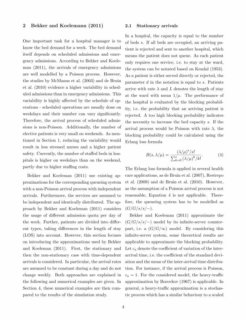
Table 1 provides the approximated blocking prob-

ability and standard deviation of the offered load for

some choices of c2a and the considered service time

distributions. For the hyper-exponential distribu-

tion, the parameters are set to p1 = 0.5, 1/µ1 = 3

and 1/µ2 = 5. The results evidence an increasing

blocking probability with increasing ca. Further-

5

Table 1: Approximated blocking probability and es-timated standard deviation of the offered load fordifferent ca.

c2a Length of stay z Bc (%)√z · λ/µ

1 Deterministic 1 5.8 4.84Exponential 1 5.8 4.84H2(p1 = 0.5) 1 5.8 4.84

2 Deterministic 2 10.1 6.85Exponential 1.5 8.5 5.93H2(p1 = 0.5) 1.48 8.4 5.90

0.5 Deterministic 0.5 2.5 3.42Exponential 0.75 4.2 4.19H2(p1 = 0.5) 0.76 4.3 4.21

more, for c2a < 1, the deterministic service time dis-

tribution leads to a lower blocking probability than

the other two. For ca > 1, this relation is the other

way round.

2.3 Time-dependent arrivals

In the following, it is assumed that the arrival rate

for each hour of the day is constant but can dif-

fer from day to day. Furthermore, the arrival rate

per day of the week does not change weekly. Con-

sequently, the arrival process can take seven differ-

ent arrival rates, one for each day. Formally, let

λ1, · · · , λ7 denote the arrival rates for the seven days

of the week with λ1 being the arrival rate at Mon-

days. Further, λ denotes the average arrival rate.

Bekker and Koeleman (2011) apply the approach

by Holtzmann and Jagerman (1979) and split up

the peakedness into a random part, zrand, and a pre-

dictable part, zpred, both depending on the arrival

process. Specifically, the predictable part comes

from the changing arrival rates whereas the random

part depends on ca. The random part of the peaked-

ness is determined by Equation 5. Formally,

z = zrand + zpred

= 1 + (c2a − 1)1

EL

∫ ∞0

P(L > y)2dy + zpred(7)

Applying the Hayward approximation, see Equation

6, and the continuous Erlang loss formula, it is noted

that the blocking probability for a non-stationary

arrival process is at least as high as the blocking

probability of the stationary arrival process with ar-

rival rate λ.

In order to estimate the predictable peakedness,

Bekker and Koeleman (2011) apply the fluid ap-

proximation by Massey and Whitt (1993). There-

fore, the parameter zpred determines as the coef-

ficient of the variance and the mean of the ex-

pected number of occupied beds in the correspond-

ing (G/G/∞) queueing system. Formally,

zpred =V ar[m(t)]

E[m(t)], (8)

where m(t) is the mean number of occupied beds in

the system at time point t.

As the arrival process is non-Poisson, Equation

2 cannot be applied directly. However, due to the

independence of the arrivals, Equation 2 can be gen-

eralised to this specific case of non-Poisson arrivals.

In particular, for a discrete time process, the ex-

pected number of patients in service at the end of

day d, d ∈ N, is determined by

m(d) = E[number in the system at day d]

=d∑

i=−∞E[arrivals day i] · P[still in service]

=

∞∑i=0

λ(d− i)P(L > i).

However, as the patients can arrive and be dis-

charged at each time of the day, the formula for

m(d) has to be formulated in continuous time. In

the continuous case, m(t) determines to

m(t) =

∫ ∞0

λ(t− y)P(L > y)dy (9)

According to the arrival rates considered, λ(t) is

defined as λ(t) = λi, if i = dte mod 7 + 1. Con-

6

sequently, the interval (d− 1, d) corresponds to the

day d.

As mentioned in Section 2.2, Bekker and Koele-

man (2011) model the service times at the ward

by a exponential or a hyper-exponential distribu-

tion. For the case of exponential service times and

d ∈ N, a recursive relation is obtained for the ex-

pected number of patients in the system, denoted

by me(d), at time point d. Formally,

me(d) =

∫ ∞0

λ(d− s)e−sµds

=

∫ 1

0λ(d)e−sµds+

∫ ∞1

λ(d− s)e−sµds

=λ(d)

µ

(1− e−µ

)+ e−µ

∫ ∞0

λ(d− s− 1)e−sµds

=λ(d)

µ

(1− e−µ

)+ e−µme(d− 1)

Iteratively applying this recursive relation yields

me(d) =(1− e−µ)

µ+

n−1∑i=0

λ(d−i)e−µi+e−µnme(d−n)

By using the periodicity of the daily arrival rates, as

λ(d+ T ) = λ(d) with T = 7, this relation simplifies

to

me(d) =1

µ

(1− e−µ

1− e−µT

) T−1∑i=0

λ(d− i)e−µi (10)

In case of a hyper-exponential distribution, m(t)

determines to

m(t) =

∫ ∞0

λ(t− s)

J∑j=1

pje−µjs

ds

=J∑j=1

pj

∫ ∞0

λ(t− s)e−µjsds

=

J∑j=1

pjmej(t),

where mej(t) is the expected number of patients at

time point t for the exponential service time distri-

bution with mean µi.

Table 2: Fraction of refused admissions for station-ary arrivals

c2a Length of stay zrand zpred Bc (%)

1 Deterministic 1 0.553 8.7Exponential 1 0.152 6.7H2(p1 = 0.5) 1 0.150 6.7

2 Deterministic 2 0.553 13Exponential 1.5 0.152 9.2H2(p1 = 0.5) 1.48 0.150 9.1

0.5 Deterministic 0.5 0.553 6.1Exponential 0.75 0.152 5.2H2(p1 = 0.5) 0.76 0.150 5.3

The coefficient of variance and mean of the ex-

pected number in the system is then determined by

zpred =1

T − 1

T∑d=1

(m(d)−m)2

m, (11)

where m =∑T

d=1m(d)/T = λ/µ.

2.4 Numerical examples

As for the stationary case, numerical examples for

the non-stationary case are run. Bekker and Koele-

man (2011) set the arrival rate on working days to

7 and 3 otherwise. This implies a mean arrival rate

of 41/7 and an average workload of 23.43. Conse-

quently, zrand is equal to the parameter z in Table

1. The mean service time is set to 1/µ = 4 as in Sec-

tion 2.2 and the same service time distributions are

considered. The approximation results in Table 2

illustrate that the influence of the time-dependency

on the blocking-probability depends immensely on

the service time distribution. In particular, if the

service time is deterministically distributed, the pre-

dictable peakedness is very high with 0.553. Expo-

nentially and hyper-exponentially distributed ser-

vice times does not differ much. In difference to

Table 1, the approximated blocking probability is

for any of the c2a higher for the deterministic than

for the other two service time distributions.

7

3 Nelson and Gerhardt (2011)

Given the numerical examples in Section 2.2 and

2.4, the results should be verified by a simulation

study. Therefore, it is necessary to simulate inter-

arrival times from a non-stationary, non-Poisson ar-

rival process with the desired properties. For this

purpose, the simulation method by Nelson and Ger-

hardt (2011) is introduced in this section and ap-

plied in Section 4. Nelson and Gerhardt (2011) ad-

dress the simulation of non-stationary, non-Poisson

processes with integrable arrival rates and a depen-

dence structure between the arrivals. Specifically,

the dependency is modelled by a geometric auto-

correlation function.

The worksheet made available by Nelson and Ger-

hardt (2011) handles the case of piece-wise constant

arrival rates. As the numerical examples in Section

2 consider the case of a constant arrival rate dur-

ing a day, the approach by Nelson and Gerhardt

(2011) is applicable. However, Nelson and Gerhardt

(2011) argue that the simulated arrival process only

captures or approximates some important charac-

teristics of the desired arrival process; in particular,

mean, variance and autocorrelation. Nevertheless,

these are the characteristics used for the approxi-

mation by Bekker and Koeleman (2011).

The simulation method proposed by Nelson and

Gerhardt (2011) generates a non-stationary, non-

Poisson arrival process with dependent arrivals in

two steps. First, a stationary non-Poisson arrival

process, the base process, is generated. Second, the

inversion method is applied to transform the sta-

tionary process into a non-stationary process. The

inversion method, for instance described by Cinlar

(1975) and Rolski and Szekli (1991) is well-known in

order to transform a stationary Poisson process into

a non-stationary Poisson process. However, Nelson

and Gerhardt (2011) prove that it is applicable in

this more general framework of non-Poisson pro-

cesses with dependent arrivals. A second popular

method used to transform stationary Poisson pro-

cesses into non-stationary Poisson processes is the

thinning method by Lewis and Shedler (1979). Nev-

ertheless, the work by Gerhardt and Nelson (2009)

implies that this method can also be used for re-

newal processes, i.e. non-Poisson processes with in-

dependent arrivals. This section is organised as fol-

lows: In Section 3.1, the notation for the following

sections is given. Section 3.2 describes the simu-

lation of the base process. Finally, inversion and

thinning methods are described in Section 3.3 and

3.4, respectively.

3.1 Notation

In the first step, inter-arrival times {Xn : n ≥ 1}of a stationary process are generated. This process

captures important features like the autocorrelation

of the desired process. The resulting arrival count

process, i.e. the number of arrivals occurred until

time point t, is denoted by

N(t) = max

{m ≥ 0 :

m∑i=1

Xi ≤ t

}.

It is assumed that N(t) is initialised in equilibrium

with X2, X3, . . . identically distributed whereas X1

has the associated equilibrium distribution. There-

fore, E[N(t)] = rt for some fixed rate r > 0. Nelson

and Gerhardt (2011) fix the parameter r to 1. The

second step of the algorithm then transforms the se-

quence of inter-arrival times of the stationary pro-

cess into the inter-arrival times {Wn : n ≥ 1} of the

desired process with integrable arrival rates. Sim-

ilarly to the stationary process, the arrival count

process I(t) is defined by

I(t) = max

{m ≥ 0 :

m∑i=1

Wi ≤ t

}.

3.2 Base process

In the first step, a stationary process with the de-

sired characteristics is simulated. In order to model

8

a non-Poisson arrival process with dependency of

the arrivals, the Markovian Arrival Process (MAP)

introduced by Lucantoni et al. (1990) is a common

example and used in several publications, e.g. Alfa

and Frigui (1996) or Ramirez-Cobo and Carrizosa

(2012). For instance, Wang et al. (2010) or Bause

and Horvath (2010) consider the problem of fitting

such models. In general Markovian Arrival Pro-

cesses can be seen as a generalisation of the phase-

type inter-arrival times.

Nelson and Gerhardt (2011) use the Markov-

MECO (Mixture of Erlangs of Common Order) ap-

proach proposed by Johnson (1998) for simulating a

stationary non-Poisson arrival process with depen-

dence structure. The Markov-MECO is a particular

case of a Markovian Arrival Process. Gerhardt and

Nelson (2009) argue that by using a MAP base pro-

cess, the process can be initialised in equilibrium,

requiring to compute the distribution of the current

state of the continuous time Markov chain in equi-

librium (Nelson and Gerhardt, 2011).

The Markov-MECO approach extends the MECO

process by Johnson and Taaffe (1989) which can

capture the first three moments of the inter-arrival

time distribution. Johnson (1998) additionally pro-

vides a control over the dependency between the ar-

rivals. In particular, the dependency is modelled by

a Markov Chain and the autocorrelation function is

geometric; for more details on the Markov-MECO

approach, see Johnson (1998). An example of a

Markov-MECO process is illustrated in Figure 2.

The current inter-arrival time has either an Ek(λ1)

or an Ek(λ2) distribution and a Markov chain gov-

erns from which distribution the next inter-arrival

time is sampled.

Although the Markov-MECO approach can han-

dle any first three moments, in the worksheet fa-

cilitated by Nelson and Gerhardt (2011), some pa-

rameters cannot be chosen by the user. The first

parameter is the mean of the base process because

it is set to 1. Nevertheless, as the process is trans-

Figure 2: The Markov chain that describes Markov-MECO inter-arrival times. Source: Nelson and Ger-hardt (2011), page 6

formed to the desired mean arrival rates in the next

step by the inversion method, this restriction does

not limit the set of arrival processes contained in

the Markov-MECO approach.

Second, the user cannot set the skewness, as this

parameter is hard to select just by intuition. Nelson

and Gerhardt (2011) fix this parameter as the third

moment of a Markovian distribution which is fully

determined by the mean and the variance. Specif-

ically, if ca < 1, the MECon distribution by Tijms

(1994) is used and a balanced hyper-exponential dis-

tribution, for example by Sauer and Chandy (1975),

otherwise (Nelson and Gerhardt, 2011). Conse-

quently, the user can choose the parameter for the

variance c2a and the dependence structure. As the

autocorrelation function is geometric, it is suffi-

cient to give the correlation between two consec-

utive arrivals, ρ1. The worksheet is available for

download at http://users.iems.northwestern.edu/

∼nelsonb/NSNR.xls.

3.3 Inversion method

The inversion method is widely used in simulations

to transform a stationary into a non-stationary Pois-

son process. However, Gerhardt and Nelson (2009)

and Nelson and Gerhardt (2011) apply this method

to transform a non-Poisson arrival process. Specif-

ically, suppose that r(t), t ≥ 0, is the desired non-

negative, integrable arrival rate for I(t). Further,

set

R(t) =

∫ t

0r(s)ds

9

and define

R−1(s) = inf {t : R(t) ≥ s}

for all s > 0. By applying this inverse func-

tion to the inter-arrival times sampled from the

base process, the stationary inter-arrival times

{Xn : n ≥ 1} are transformed to the inter-arrival

times {Wn : n ≥ 1} and arrival times {Vn : n ≥ 1}.Formalising this procedure leads to Algorithm 1.

Algorithm 1 Inversion Method for arrival pro-cessesRequire: Inter-arrival times {Xn : n ≥ 0}Require: Integrated arrival rate R(t)1: Set W0 = 0, m = 0, V0 = 0 and S0 = 02: while Further arrivals do3: Set m = m+ 14: Set Sm = Xm + Sm−15: Set Vm = R−1(Sm)6: Set Wm = Vm − Vm−17: end while8: return Inter-arrival times {Wn : n ≥ 1}9: return Arrival times {Vn : n ≥ 1}

Figure 3 illustrates the algorithm for r(t) = 2t, i.e.

the mean arrival rate increases with constant rate

over time. The circles on the left vertical axis are the

simulated arrival times of the base process. Then

the inversion method is run on these and the crosses

on the horizontal bottom axis are the transformed

arrivals.

However, the inversion method does not automat-

ically imply that the transformed arrival counting

process I(t) is non-stationary with the desired char-

acteristics. In particular, it is necessary to exclude

that the transformed process is Poisson. For this

reason, Nelson and Gerhardt (2011) considers the

index of dispersion for counts (IDC), e.g. used in

Sriram and Whitt (1986) or Kim (2011). The IDC

of the base process N(t) is given by

IDC = limt→∞

V ar[N(t)]

E[N(t)]. (12)

Figure 3: Illustration of the inversion method withr(t) = 2t.

For example, if N(t) is a Poisson process, the IDC

is 1. Therefore, it can be concluded that the trans-

formed process I(t) is non-Poisson if the correspond-

ing index of dispersion for counts is not 1. Nel-

son and Gerhardt (2011) prove that this property is

given for the inversion method.

Theorem 1. E[I(t)] = R(t), for all t ≥ 0, and

V ar[I(t)] ≈ IDC·R(t), for large t.

Proof by Nelson and Gerhardt (2011).

The assumption that N(t) is initialised in equilib-

rium with rate r = 1 implies E[N(t)] = t, for all

t ≥ 0. Further, because of equation 12, V ar[N(t)] ≈IDC · t, for large t. Thus

E[I(t)] = E[E {I(t)|N(R(t))}]

= E[N(R(t))]

= R(t)

for all t ≥ 0, while

V ar[I(t)] = E[V ar {I(t)|N(R(t))}]+

V ar [E {I(t)|N(R(t))}]

= 0 + V ar[N(R(t))]

≈ IDC ·R(t)

for large t.

10

Thus Theorem 1 implies that the transformed

process I(t) has approximately the same IDC as

the base process N(t). Consequently, if the simu-

lated, stationary arrival process has an IDC which

is significantly different from 1, the transformed

non-stationary process preserves this property and

is thus non-Poisson. In the same way, the result

implies that the non-stationary process generated

by applying the inversion method to a stationary

Poisson process is also Poisson. In summary, apply-

ing the inversion method leads to the desired arrival

rate under preserving the IDC. The worksheet facil-

itated by Nelson and Gerhardt (2011) works with

piecewise-constant arrival rates which have to be

specified by the user. Finally, the user has to set the

length of the simulation and the number of replica-

tions to run. The simulated inter-arrivals times are

then wrote in a Excel-spreadsheet with one replica-

tion per column and can be used for the simulation.

Nelson and Gerhardt (2011) mention that the

IDC is not a quite intuitive measure of variability

and dependence. Therefore, the authors also con-

sider the index of dispersion for intervals (IDI) by

Gusella (1991). Formally, the IDI is given by

IDI = limn→∞

V ar[∑n

i=1Xi]

nE2[X2]

=c2a

1 + 2∞∑j=1

ρj

,

where ρj is the lag-j autocorrelation of the station-

ary inter-arrival times X2, X3, . . .. The work by

Whitt (2002) proves that both indexes are identi-

cal under some conditions. Specifically, the IDC

exists and is equal to the IDI if∑n

i=1Xi of the base

process N(t) satisfy a Central Limit Theorem of the

form1√n

(n∑i=1

Xn − nµ

)D→ N (0, τ2).

Consequently, the IDC captures both, dependency

and variability of the arrivals.

3.4 Thinning method

Another approach used in simulations to transform

a stationary to a non-stationary Poisson process

is the thinning method. The work by Gerhardt

and Nelson (2009) proves that the thinning method

is also applicable to transform a stationary, non-

Poisson process to a non-stationary non-Poisson un-

der the condition that the arrivals are independent.

In particular, let r∗ = max {r(t) : t ≥ 0} be the

maximum arrival rate occurring and assume that

r∗ is finite.

The first step is again to simulate the inter-arrival

times {Xn : n ≥ 1} of a stationary non-Poisson pro-

cess with arrival rate r∗ and variance c2a/(r∗)2, i.e.

the inter-arrival distribution has mean 1/r∗ and

variance c2a/(r∗)2 (Gerhardt and Nelson, 2009). For

instance, the MECO process by Johnson and Taaffe

(1989) could be used again. After simulating this

stationary process, a simulated arrival at time point

t is accepted with probability r(t)/r∗, i.e. if r(t) =

r∗, all sampled arrivals are accepted. Otherwise,

the simulated arrival time is rejected and does not

appear in the transformed arrival process. This ap-

proach leads to Algorithm 2.

Algorithm 2 Thinning Method for non-stationaryarrival processes

Require: Inter-arrival times {Xn : n ≥ 1}Require: Arrival rate r(t)1: Set r∗ = max {r(t) : t ≥ 0}2: Set m = 0, p = 0, V0 = 0, W0 = 0 and S0 = 03: while Further arrivals do4: Set m = m+ 15: Set Sm = Xm + Sm−16: Generate Um ∼ Uniform[0, 1]7: if Um < r(Sm)/r∗ then8: Set p = p+ 19: Set Vp = Sm

10: Set Wp = Vp − Vp−111: end if12: end while13: return Inter-arrival times {Wn : t ≥ 1}14: return Arrival times {Vn : n ≥ 1}

11

Figure 4: Illustration of the thinning method withpiecewise-linear arrival rates with accepted arrival(red) and rejected arrivals (black).

Figure 4 illustrates a resulting arrival process with

piecewise-constant arrival rates and r∗ = 4.8. The

red crosses are the generated and accepted arrivals

and the black crosses are generated by the non-

stationary arrival process but rejected. Gerhardt

and Nelson (2009) prove that E[I(t)] = R(t) for

all t ≥ 0. Further, Gerhardt and Nelson (2009)

prove that the index of dispersion for counts of the

transformed process I(t) at time point t can be ap-

proximated; see Result 2.3 of Gerhardt and Nelson

(2009). Gerhardt and Nelson (2009) use Phase-type

distributions to simulate the stationary non-Poisson

process. Phase-type distributions are widely used to

fit renewal processes, see for instance Harper et al.

(2011) or Payne et al. (2012). However, as the sim-

ulation study in Section 4 is based on the work-

sheet by Nelson and Gerhardt (2011), the thinning

method is not considered in more detail.

This section concludes by mentioning that the

processes generated by thinning and inversion are

not equivalent in general as an example by Gerhardt

and Nelson (2009) evidences. Consider R(t) = t/2,

i.e. r(t) = 1/2, and the base process has rate 1.

Then the expectation of the process generated by

inversion is 2n+ c2a− 1. Otherwise, the expectation

of the process generated by thinning is 2n+ c2a−12 .

4 Simulation Study

The numerical examples in Section 2 evidence two

results. First, the blocking probability increases

with the variance of the arrival process. Second,

a non-stationary arrival process leads to a higher

blocking probability than a stationary arrival pro-

cess with the same mean arrival rate. In order to

evaluate the approximations obtained in Section 2.2

and 2.4, several simulations are run. Nevertheless,

the approximations do not consider the case of de-

pendent arrivals. Therefore, the sensitivity of the

blocking probability on positive and negative corre-

lation is investigated. Another not considered as-

pect is the possibility of batched arrivals. For in-

stance, in case of a car accident with several casu-

alties, family members are normally taken to the

same hospital. This case is as well investigated by

simulation.

Following the setting in Section 2, the bed capac-

ity is fixed at s = 28 beds and the average length

of stay is four days. In particular, the service time

distributions considered are the deterministic, the

exponential and the hyper-exponential distribution.

Here, the hyper-exponential distribution is the mix-

ture of two exponential distributions with parame-

ter µ1 = 3, µ2 = 5 and p1 = 0.5.

The samples of the arrival processes are generated

by the worksheet facilitated by Nelson and Gerhardt

(2011). Each arrival process is the union of ten ar-

rival processes of run length 365 days, i.e. the total

run length is about 10 years. Due to overflow prob-

lems, the worksheet cannot handle a time period of

more than 3000 days. All simulations are run in

Simul8 and the generated samples are imported as

csv-files. To avoid incorrectness, a warm-up period

of 10 days is set. In the simulation, a patient queues

at maximum 15 minutes, although the setting in

Section 2 states that the patient leaves automati-

cally. However, the results of the simulated queue

indicate that the number of patients which get a bed

12

Table 3: Approximated and simulated blockingprobability for stationary independent arrivals anddifferent choices of c2a.

c2a Length of stay approx.(%) simul. (%)

1 Deterministic 5.8 5.7Exponential 5.8 5.7H2(p1 = 0.5) 5.8 5.7


0.5 Deterministic 2.5 3.0Exponential 4.2 4.4H2(p1 = 0.5) 4.3 4.4

because they wait 15 minutes is negligible. In order

to achieve valid results, for each arrival process and

each length of stay distribution, ten repetitions are

run and the blocking probability is taken as the av-

erage number of rejected patients and divided by the

number of arrived patients. The Simul8 worksheet

and all generated arrival processes are available for

download at http://www.lancs.ac.uk/pg/rohrbeck/

simulation-project.zip.

This section is organised as follows: First in Sec-

tion 4.1, the blocking probability of the stationary

case is simulated and compared to the approximated

results of Section 2.2. Then the case of slightly pos-

itive or negative correlated arrivals is considered.

Section 4.2 considers the case of non-stationary ar-

rivals in the same way as Section 4.1. Finally, Sec-

tion 4.3 investigates whether it is important to con-

sider batched arrivals or not in this setting.

4.1 Stationary arrivals

According to the numerical examples in Section 2.2,

the arrival rate per day is set to λ = 41/7. Addition-

ally, the arrivals are independent. Table 3 provides

the approximated and simulated blocking probabil-

ities for this setting. The results evidence that the

approximation fits the simulated blocking probabil-

ity very well. In particular, the largest difference

of 0.5 occurs for c2a = 0.4 and deterministically dis-

tributed service times.

All the properties concluded by the approxima-

tions are approved by the simulations. First, the

blocking probability increases with the coefficient of

variation ca. Second, the deterministic service time

distribution is more sensitive to changes in variance

than the other two considered distributions. Sen-

sitivity in this context refers to the relative change

of the blocking probability with changing ca. How-

ever, also the absolute change is higher. Third, the

blocking probability for c2a = 1 is equal for each

of the three considered service time distributions.

Property two and three imply that for c2a < 1,

the deterministic service time distribution implies

a lower blocking probability than the other two dis-

tributions. For c2a > 1, the relation is the opposite

way round. Forth,the difference between exponen-

tial and hyper-exponential distributed service times

is small.

Next, the sensitivity of the blocking probability

on possible dependency in the arrival process, pos-

itive as well as negative, is investigated. In order

to compare this setting to the one in Section 2.2,

the same service time distributions and values for

c2a as in Table 3 are considered. In difference to the

previous simulations, the parameter value ρ1 of the

geometric autocorrelation function is not equal 0. In

particular, in order to model positive correlation, ρ1

is set to 0.2. Otherwise, ρ1 is set to -0.2 for negative

correlation. For c2a = 2, ρ1 = −0.2 is not contained

in the feasible region of the worksheet by Nelson

and Gerhardt (2011). In this case, ρ1 is set to the

smallest possible value, ρ1 = −0.085. Consequently,

six different arrival processes are generated, two for

each value of c2a.

Table 4 provides the blocking probabilities for the

considered parameter settings. Several conclusions

are drawn from this results. First, the higher ρ1,

the higher the blocking probability. In particular,

if the arrivals are negatively correlated, the block-

13

Table 4: Simulated blocking probability for positiveand negative correlated, stationary arrivals and dif-ferent choices of c2a.

c2a ρ1 Length of stay simulated Bc(%)

1 -0.2 Deterministic 4.5Exponential 5.1H2(p1 = 0.5) 5.2

0.2 Deterministic 9.9Exponential 8.3H2(p1 = 0.5) 8.4



0.5 -0.2 Deterministic 2.0Exponential 3.9H2(p1 = 0.5) 3.9


ing probability is lower than in the case of indepen-

dent arrivals. Contrary, positive correlated arrivals

lead to a higher blocking probability. Especially if

c2a = 2, the absolute change in per cent is large. In

other words, the more the arrivals are correlated,

the higher is the number of rejected patients.

Second, the absolute difference in the blocking

probability between the negative correlated and the

independent arrivals is lower than the absolute dif-

ference between the positive correlated and indepen-

dent arrivals. For instance, for c2a = 1 and the de-

terministic distribution, the absolute difference be-

tween negative correlated and independent arrivals

is 1.2%. On the other hand, the absolute differ-

ence between positive correlated and independent

arrivals is 4.2%. Thus, the blocking probability is

more sensitive to positive than to negative correla-

tion. Third, independent of the correlation of the

arrivals, a higher c2a leads to a higher blocking prob-

ability. Therefore, the property concluded by the

approximations is valid for correlated arrival pro-

cesses too. Forth, the blocking probabilities for ex-

ponentially and hyper-exponentially distributed ser-

vice times are similar though the blocking probabil-

ity for the exponential service time distribution is

often smaller.

Last, the deterministic service time distribution

is more sensitive to correlation than the other two

service time distributions; e.g. for c2a = 1 the rel-

ative difference between positive correlated and in-

dependent arrivals is 74% whereas it is 46% for the

exponential distribution. Another example is that

the blocking probability of the determisitc distribu-

tion for c2a = 0.5 and ρ1 = 0.2 is higher than for the

exponential distribution although it is the other way

around for ρ1 = 0. On the other hand, for c2a = 1

and ρ1 = −0.2, the deterministic distribution leads

to a lower blocking probability than the exponen-

tial distribution although the blocking probabilities

were equal for ρ1 = 0. In summary, correlation has a

high influence on the blocking probability. However,

the degree of influence depends on the service time

distribution. The determinsitic service time distri-

bution in particular is highly sensitive to changes in

the dependence structure of the arrival process.

4.2 Non-stationary arrivals

The theoretical results of Section 2.3 imply an

higher blocking probability for non-stationary ar-

rivals than for stationary arrivals with the same av-

erage arrival rate. The impact of time-dependent

arrivals has been observed in various studies, for

instance by Melamed et al. (1992) on compressed

video frame bits and by Ware et al. (1998) on com-

puter networks. For example, Biller and Nelson

(2005) introduce an approach to fit stochastic mod-

els to dependent time-series processes inputs.

According to Section 2.4, the mean arrival rate

is set to 7 patients per day on working days and 3

per day on the weekend. This implies an average

arrival rate of λ = 41/7. First, the case of inde-

14

Table 5: Approximated and simulated blockingprobability for non-stationary independent arrivalsand different choices of c2a.

c2a Length of stay approx.(%) simul. (%)




pendent arrivals is considered. Table 5 provides the

simulated and approximated blocking probabilities

for the considered arrival processes with different

values for c2a. Compared to Table 3, the simulated

blocking probability is higher for the non-stationary

than for the stationary case. Consequently, the sec-

ond conclusion of Section 2 is approved by the sim-

ulation.

As for the stationary case, the blocking proba-

bility increases with c2a. Further, the results con-

firm that the deterministic service time distribution

leads to higher blocking probabilities than the other

two service time distributions for any of the consid-

ered values for c2a and is thus more sensitive to non-

stationarity. As in Table 3, the difference between

the exponential and hyper-exponential service time

distributions is very small. However, in difference

to Table 3, the difference between simulated and

approximated blocking probability is higher. This

effect may be due to the higher number of approx-

imations used in the non-stationary case, e.g. the

fluid approximation for calculating the predictable

peakedness. Nevertheless, the approximations fit

the simulated blocking probabilities quite well.

After investigating the case of independent ar-

rivals, the case of dependent arrivals is considered in

the following. The parameter values for ρ1 are set to

Table 6: Simulated blocking probability for positiveand negative correlated, non-stationary arrivals anddifferent choices of c2a.

c2a ρ1 Length of stay simulated Bc(%)





0.5 -0.2 Deterministic 6.4Exponential 5.1H2(p1 = 0.5) 5.0


the same values as in Section 4.1, i.e. negative and

positive correlated arrivals are simulated. Although

the influence of dependency of the arrivals was al-

ready studied in Section 4.1, it is not clear how large

the combined effect of non-stationarity and depen-

dency is. In particular, the correlation between de-

pendency of the arrivals and a non-stationary arrival

process is investigated. Table 6 provides the simu-

lated blocking probabilities for non-stationary ar-

rival processes with dependent arrivals for the three

considered service time distributions.

Several results obtained in Section 4.1 are also

valid for this case. First, the blocking probability

for a non-stationary arrival process increases with

ρ1 and c2a. Second, the blocking probability is more

sensitive to positive than to negative autocorrela-

tion. For instance, for the case of c2a = 0.5 and

deterministic service time distribution, the simu-

lated blocking probability is 43% higher if ρ1 is 0.2

than for the independent case in Table 5. On the

15

other hand, the blocking probability decreases by

9% if the parameter ρ1 is −0.2. Third, the deter-

ministic distribution is more sensitive to correlation

than the exponential or hyper-exponential distribu-

tion. Last, as in all simulations before, the differ-

ence between exponential and hyper-expoential ser-

vice time distribution is not high.

Additionally to these results, further conclusions

can be found about the influence of the non-

stationarity. First, the relative change caused by

the dependency in the arrival process in the non-

stationary case is less than in the stationary case;

e.g. for c2a = 1 and the exponential distribution, the

relative difference between independent and posi-

tive correlated arrivals is 46% in the stationary case

whereas it is 34% in the non-stationary case. In

other words, if the arrival process is non-stationary,

the blocking probability is less sensitive to depen-

dency.

Second, a higher value of ρ1 decreases the rel-

ative difference between the stationary and non-

stationary arrival process. For instance, for the

deterministic service time distribution, the rela-

tive difference between the stationary and the non-

stationary case is 63% for c2a = 1 and ρ1 = 0 , but

25% for c2a = 1 and ρ1 = 0.2. The same result holds

for c2a. These observations can be formulated in the

following two points for the considered service time

distributions:

1. The higher c2a, the less sensitive is the block-

ing probability to non-stationarity of the arrival

process.

2. The higher ρ1, the less sensitive is the block-

ing probability to non-stationarity of the arrival

process.

In summary, the non-stationarity of the arrival

process increases the blocking probability compared

to the stationary case. On the other hand, the

blocking probability is less sensitive to changes in

the variability or dependency of the arrival process.

Table 7: Approximated and simulated blockingprobability for stationary independent arrivals anddifferent choices of c2a for the case of batched arrivalsand not batched arrivals.

c2a Length of stay no batches batches




4.3 Batches of arrivals

All the approximations considered so far assume

that patients arrive single. The simulations done

in Section 4.1 and Section 4.2 evidence an high im-

portance to know whether the arrivals are truly in-

dependent. In the previous sections, dependency

was modelled by a geometric autocorrelation func-

tion. Here, the dependency is considered to be in

the form that some patients arrive in batches. As

the worksheet does not give the opportunity to sim-

ulate such arrival processes, they are generated by

rounding up the arrival times generated for Table

3. In particular, the day is split up into intervals of

2.5 hours length and arrivals in one interval arrive

at the same time. This leads to batches of size two

or three at some time points.

Table 7 provides the simulated blocking probabil-

ities for the case of batched arrivals. The results evi-

dence a small difference between the case of batched

arrivals and the case of independent arrivals. How-

ever, the difference is not significant. Therefore, it

is concluded that the possibility of small batches of

arrivals has not to be considered in this application.

All other properties concluded from Table 3 can be

also approved for the case of batched arrivals.

16

5 Summary and Discussion

The motivation for this work was to investigate

the impact of non-Poisson arrival processes on the

blocking probability of a (G/G/s/s/−) model. In

particular, the impact of variance, non-stationarity

and dependency was considered. Studies in health

care applications motivate the necessity to consider

such systems with non-Poisson arrival processes.

McManus et al. (2003), for example, evidence that

the arrivals of scheduled admissions at a clinical

ward is not well modelled by a Poisson process.

Bekker and Koeleman (2011) consider indepen-

dent, non-Poisson arrivals and approximate the cor-

responding queueing system by a (G/G/∞) model.

However, possible dependency in the arrival pro-

cess is not investigated, The blocking probability

is then estimated by applying the Hayward ap-

proximation and the heavy-traffic approximation by

Borovkov (1967). For the non-stationarity arrival

process, the fluid approximation is used addition-

ally. In order to measure the impact of variation and

non-stationarity, the approximations were applied

to several service time distributions and arrival pro-

cesses with equal mean but different variability. The

theoretical results implied that the blocking proba-

bility is higher for non-stationary arrival processes

and increases with the variation of the arrival pro-

cess. Furthermore, the sensitivity to the variance

depends on the service time distribution. Bekker

and Koeleman (2011) also considers shortly the case

of health chains, i.e. systems with more than one

ward. In this case, heavy-traffic approximations ex-

ist too, e.g. see Glynn and Whitt (1991). However,

these have a more complicated form than the ap-

proximation considered here.

In the simulation studies, the worksheet by Nel-

son and Gerhardt (2011) was then used to simu-

late non-Poisson arrival processes which captured

the features considered by Bekker and Koeleman

(2011); mean, variance and non-stationarity. The

approach by Nelson and Gerhardt (2011) samples

inter-arrival times from a Markov-MECO process

which can capture the first three moments of the de-

sired inter-arrival time distribution. Furthermore,

Markov-MECO allows to model dependency be-

tween the arrivals by a geometric autocorrelation

function. By using the inversion method, the simu-

lated inter-arrival times are then transformed to the

desired non-stationary arrival process. The possibil-

ity of dependency of the arrivals was also used, in

order to investigate the sensitivity of the blocking

probability to dependency between the arrivals.

However, whether the Markov-MECO approach

is always appropriate to model the arrival process is

unsure. The knowledge which descriptors are most

important to approximate the arrival process suffi-

ciently, is still limited (Johnson and Taaffe, 1989).

The work by Anderson et al. (2004) evidence that

an Markovian Arrival process and its reverse can-

not be distinguished properly by classical statistical

descriptors like mean, variance, etc. Additionally,

several authors propose new descriptors for arrival

processes. Johnson and Narayana (1996), for ex-

ample, proposes new descriptors of burstiness of a

Markovian arrival processes. Therefore, further re-

search is needed to specify which descriptors are re-

quired under which conditions to model the arrival

process sufficiently in order to approximate the de-

sired properties of the queueing system.

The simulated blocking probabilities approved

the approximations for all considered cases. Fur-

ther, the influence of possible dependency between

the arrivals on the blocking probability was investi-

gated. The results implied that the blocking prob-

ability increases with the dependency in the arrival

process. This means, a positive correlation between

the arrivals led to a higher blocking probability com-

pared to the case of independent arrivals. In the

same way, negative correlated arrivals led to a lower

blocking probability. Last, the case of batched ar-

rivals was considered and the results evidenced that

17

small batches do not have to be modelled in the

considered setting.

However, further research is still necessary. First,

as the simulation study evidences that a depen-

dency between the arrivals has a high impact on

the blocking probability, it is necessary to find a

closed form approximation for the case of depen-

dent arrivals. Following the Hayward approxima-

tion, one approach may be to extend the formula

of the peakedness in the heavy-traffic approxima-

tion by a factor for the autocorrelation between the

arrivals. Second, Bekker and Koeleman (2011) use

the fluid approximation to model the non-stationary

case. Nevertheless, the simulation results indicate

that there may exist a better approach to capture

the non-stationarity.

Third, Gerhardt and Nelson (2009) also propose

the thinning method to transform independent non-

Poisson arrivals. However, it is not clear whether

this method can also be applied to dependent ar-

rivals in the way that an index measure, such as the

IDC, is preserved. Forth, as the number of staffed

beds varies during a week, it is necessary to inves-

tigate whether the variation of the capacity has a

high impact on the blocking probability or whether

the blocking probability is possibly reduced due to

a higher capacity during days of high admission.

This work considered the problem of modelling

arrival processes in health care applications with re-

spect to finite capacity. The consideration of non-

Poisson arrival processes in health care applications

is of great importance as shown by several stud-

ies. For the considered setting, methods to approx-

imate or simulate the performance of the system

exist. Specifically, the approaches by Bekker and

Koeleman (2011) and Nelson and Gerhardt (2011)

lead to good results. In the framework of time-

dependent arrival rates, both approaches are appli-

cable and imply the same conclusions, an increas-

ing blocking probability with increasing variance

and non-stationarity of the arrival process. How-

ever, the theoretical approximations by Bekker and

Koeleman (2011) ignore a possible dependency of

the arrivals which has a significant influence on the

blocking probability, as evidenced by the simulation

study performed in this work.

References

Alfa, A. S. and Frigui, I. (1996). Discrete NT-policy

single server queue with markovian arrival process

and phase type service. European Journal of Op-

erational Research, 88(3):599–613.

Anderson, A. T., Neuts, M. F., and Nielsen, B. F.

(2004). On the time reversal of Markovian arrival

processes. Stochastic Models, 20(2):237–260.

Bause, F. and Horvath, G. (2010). Fitting Marko-

vian Arrival Processes by incorporating correla-

tion into phase type renewal processes. In 7th

International Conference on Quantitative Evalu-

ation of SysTems (QEST) 2010, pages 97–106.

Bekker, R. and Koeleman, P. M. (2011). Schedul-

ing admissions and reducing variability in bed

demand. Health Care Management Science,

14(3):237–249.

Biller, B. and Nelson, B. L. (2005). Fitting time-

series input processes for simulation. Operations

Research, 53(3):549–559.

Bodenheimer, T. (2005). High and rising health care

costs. Part 2: technologic innovation. Annals of

internal medicine, 142(11):932–937.

Borovkov, A. (1967). On limit laws for service pro-

cesses in multi-channel systems. Siberian Mathe-

matical Journal, 8(5):746–763.

Cinlar, E. (1975). Introduction to stochastic pro-

cesses. Prentice-Hall, Englewood Cliffs, NJ.

Creemers, S. and Lambrecht, M. (2009). Queueing

models for appointment-driven systems. Annals

of Operation Research, 178(1):155–172.

18

de Bruin, A., Bekker, R., van Zanten, L., and Koole,

G. (2010). Dimensioning clinical wards using the

Erlang loss model. Operations Research, 178:23–

43.

de Bruin, A. M., van Rossum, A. C., m C, V., and

Koole, G. M. (2007). Modeling the emergency

cardiac in-patient flow: an application of queu-

ing theory. Health Care Management Science,

10(2):125–137.

Deo, S. and Itai, G. (2011). Centralized vs. decen-

tralized ambulance diversion: A network perspec-

tive. Management Science, 57(7):1300–1319.

Fontantesi, J., Alexopoulos, C., Goldsman, D.,

DeGuire, M., Kopald, D., Holcomb, K., and

Sawyer, M. (2002). Non-punctual patients:

planning for variability in appointment arrival

times. Journal of Medical Practice Management,

18(1):14–18.

Gerhardt, I. and Nelson, B. (2009). Transform-

ing renewal process for simulation of nonstation-

ary arrival processes. Journal on Computing,

21(4):630–640.

Glynn, P. W. and Whitt, W. (1991). A new view

of the heavy-traffic limit theorem for infinite-

server queues. Advances in Applied Probability,

23(1):188–209.

Gross, D. and Harris, C. M. (1985). Fundamentals

of Queueing Theory. Wiley, New York, 2 edition.

Gusella, R. (1991). Characterizing the variability of

arrival processes with indexes of dispersion. IEEE

Journal On Selected Areas In Communications,

9(2):203–211.

Harper, P. R., Knight, V. A., and Marshall, A. H.

(2011). Discrete conditional phase-type models

utilising classification trees: Application to mod-

elling health service capacities. European Journal

of Operational Research, 219(3):522–530.

Holtzmann, J. and Jagerman, D. (1979). Estimating

peakedness from arrival counts. In Proceedings of

ITC-9. Torremolinos, Spain.

Izady, N. and Worthington, D. (2012). Setting

staffing requirements for the time dependent

queueing networks: The case of accident and

emergency departments. European Journal of Op-

erations Research, 219(3):531–540.

Jackson, J. (1957). Networks of waiting lines. Op-

erations Research, 5(4):518–521.

Jagers, A. A. and Van Doorn, E. A. (1986). On

the continued Erlang loss function. Operations

Research Letters, 5(1):43–46.

Johnson, M. A. (1998). Markov MECO: a simple

markovian model for approximating nonrenewal

arrival processes. Stochastic Models, 14(1-2):419–

442.

Johnson, M. A. and Narayana, S. (1996). Descrip-

tors of arrival-process burstiness with application

to the discrete Markovian arrival process. Queue-

ing Systems, 23(1):107–130.

Johnson, M. A. and Taaffe, M. R. (1989). Match-

ing moments to phase distributions: Mixture of

Erlangs of common order. Stochastic Models,

5(4):711–743.

Kendal, D. (1953). Stochastic processes occurring

in the theory of queues and their analysis by the

method of the imbedded markov chain. The An-

nals of Mathematical Statistics, 24(3):338–354.

Kim, S. (2011). The two-moment three-parameter

decomposition approximation of queueing net-

works with exponential residual renewal pro-

cesses. Queueing Systems, 68(2):193–216.

Lane, D., Monefeldt, C., and Rosenhead, J. (2000).

Looking in the wrong place for healthcare im-

provements: A system dynamics study of an ac-

19

cident and emergency department. Journal of the

Operational Research Society, 51(5):518–531.

Lewis, P. A. W. and Shedler, G. S. (1979). Sim-

ulation of nonhomogeneous Poisson processes by

thinning. Naval Research Logistics Quarterly, 26.

Little, J. D. C. (1961). A proof for the queueing

formula L= λW. Operations Research, 9:383–387.

Litvak, E., Buerhaus, P., Davidoff, F., and Long,

M. (2005). Managing unnecessary variability in

patient demand to reduce nursing stress and im-

prove patient safety. Joint Commission on quality

and patient safety, 31(6):330–338.

Lucantoni, D. M., Meier-Hellstern, K. S., and

Neuts, M. F. (1990). A single-server queue with

server vacations and a class of non-renewal ar-

rival processes. Advances in Applied Probability,

22(3):676–705.

Massey, W. and Whitt, W. (1993). Networks of

infinite-server queues with nonstationary Poisson

input. Queueing Systems, 13(1):183–250.

McManus, M., Long, M., Copper, A., Mandell, J.,

Berwick, D., Pagano, M., and Litvak, E. (2003).

Variability in surgical caseload and access to in-

tensive care services. Anesthesiology, 98(6):1491–

1496.

Melamed, B., Hill, J. R., and Goldsman, D. (1992).

The TES methodology: Modeling empirical sta-

tionary time series. In Swain, J. J., Goldsman,

D., Crain, R. C., and Wilson, J. R., editors, Proc.

1992 Winter Simulation Conference, pages 135–

144, Institute of Electrical and Electronics Engi-

neers, Piscataway, NJ.

Nelson, B. and Gerhardt, I. (2011). Modelling and

simulating non-stationary arrival processes to fa-

cilitate analysis. Journal of Simulation, 5:3–8.

Payne, K., Marshall, A. H., and Cairns, K. J.

(2012). Investigating the efficiency of fitting

Coxian phase-type distributions to health care

data. IMA Journal of Management Mathemat-

ics, 23(2):133–145.

Ramirez-Cobo, P. and Carrizosa, E. (2012). A

note on the dependence structure of the two-state

Markovian arrival process. Journal of Applied

Probability, 49(1):295–302.

Restrepo, M., Henderson, S. G., and Topaloglu, H.

(2009). Erlang loss models for the static deploy-

ment of ambulances. Health Care Management

Science, 12(1):67–79.

Rolski, T. and Szekli, R. (1991). Stochastic order-

ing and thinning. Stochastic Processes and their

Applications, 37(2):299–312.

Sauer, C. and Chandy, K. (1975). Approximate

analysis of central server models. IBM Journal

of Research and Development, 19(3):301–313.

Seshamani, M. and Gray, A. (2004). Time to death

and health expenditure: an improved model for

the impact of demographic change on the health

care costs. Age and Ageing, 33(6):556–561.

Singh, V. (2006). Use of queuing models in health

care. http://works.bepress.com/vikas singh/4/.

Sriram, K. and Whitt, W. (1986). Characterizing

superposition arrivals processes in packet multi-

plexers for voice and data. IEEE Journal on Se-

lected Areas in Communications, 4(6):833–846.

Tijms, H. C. (1994). Stochastic Models: An Algo-

rithmic Approach. Wiley, New York.

Wang, X., Qu, H., Xu, L., Han, X., and Zhang,

J. (2010). A MAP fitting approach with joint

approximation oriented to the dynamic resource

provisioning in shared data centres. In 2010 Fifth

International Conference on Networking, Archi-

tecture, and Storage, pages 100–108.

20

Ware, P. P., Page, T. W., and Nelson, B. L. (1998).

Automatic modeling of file system workloads us-

ing two-level arrival processes. ACM Trans-

actions on Modeling and Computer Simulation

(TOMACS), 8(3):305–330.

Whitt, W. (1984). Heavy-traffic approximations for

service systems with blocking. AT&T Bell Labo-

ratories Technical Journal, 63(5):689–708.

Whitt, W. (1992). Understanding the efficiency of

multi-server service systems. Management Sci-

ence, 38(5):708–723.

Whitt, W. (2002). Stochastic-Process Limits: An

Introduction to stochastic process limits and their

application to queues. Springer, New York.

Worthington, D. (2009). Reflections on queue mod-

elling from the last 50 years. Journal of the Op-

erational Research Society, 60:S82–S93.

21

Documents

The Impact of non-Poisson Arrival Processes in Health · PDF fileThe Impact of non-Poisson Arrival Processes in Health Care Facilities with Finite Capacity Christian Rohrbeck Supervisor: