Embed Size (px)
Citation preview

DI
SC
US
SI
ON
P
AP
ER
S
ER
IE
S
Forschungsinstitut zur Zukunft der ArbeitInstitute for the Study of Labor
The Impact of Managerial Change on Performance:The Role of Team Heterogeneity
IZA DP No. 6884
September 2012
Sandra HentschelGerd MuehlheusserDirk Sliwka

The Impact of Managerial Change on Performance:
The Role of Team Heterogeneity
Sandra Hentschel Bielefeld University
Gerd Muehlheusser
University of Hamburg, IZA and CESifo
Dirk Sliwka
University of Cologne, IZA and CESifo
Discussion Paper No. 6884 September 2012
IZA
P.O. Box 7240 53072 Bonn
Germany
Phone: +49-228-3894-0 Fax: +49-228-3894-180
E-mail: [email protected]
Any opinions expressed here are those of the author(s) and not those of IZA. Research published in this series may include views on policy, but the institute itself takes no institutional policy positions. The IZA research network is committed to the IZA Guiding Principles of Research Integrity. The Institute for the Study of Labor (IZA) in Bonn is a local and virtual international research center and a place of communication between science, politics and business. IZA is an independent nonprofit organization supported by Deutsche Post Foundation. The center is associated with the University of Bonn and offers a stimulating research environment through its international network, workshops and conferences, data service, project support, research visits and doctoral program. IZA engages in (i) original and internationally competitive research in all fields of labor economics, (ii) development of policy concepts, and (iii) dissemination of research results and concepts to the interested public. IZA Discussion Papers often represent preliminary work and are circulated to encourage discussion. Citation of such a paper should account for its provisional character. A revised version may be available directly from the author.

IZA Discussion Paper No. 6884 September 2012
ABSTRACT
The Impact of Managerial Change on Performance: The Role of Team Heterogeneity*
When a key responsibility of a manager is to allocate more or less attractive tasks to subordinates, these subordinates have an incentive to work hard and demonstrate their talents. As a new manager is less well acquainted with these talents this incentive mechanism is reinvigorated after a management change – but only when the team is sufficiently homogenous. Otherwise, a new manager quickly makes similar choices as the old one did. We investigate this hypothesis using a large data set on coach dismissals in the German football league where the selection of players is indeed a key task of the coach. Indeed, we find substantial evidence that coach replacements enhance team performance (only) in homogenous teams. Moreover, from a methodological point of view, we argue that there is typically a negative selection bias when evaluating succession effects, which might reconcile previous findings of no (or even negative) effects with the vast number of dismissals observed in reality. JEL Classification: D22, J44, J63 Keywords: managerial succession, teams, heterogeneity, tournaments Corresponding author: Gerd Muehlheusser University of Hamburg Department of Economics von-Melle-Park 5 20146 Hamburg Germany E-mail: [email protected]
* Financial support from the State of North Rhine-Westphalia (NRW), Ministry for Family, Children, Culture and Sport (MFKJKS) is gratefully acknowledged. Moreover, we thank Impire AG for kindly providing a large part of the data used in the paper and Merle Gregor, Michaela Buscha, Stefanie Kramer, Dennis Baufeld, Dennis Hebben, and Uwe Blank for excellent research assistance. We also benefitted from the comments received when presenting the paper at the 2012 workshop on “Personnel Economics” (PÖK) at the University of Paderborn, as well as the workshop on “Football and Finance” at the University of Münster.

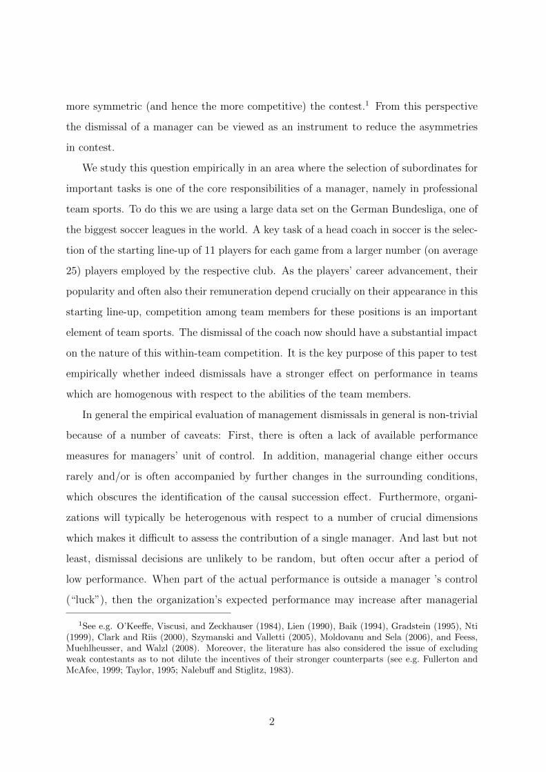
1 Introduction
In many organizations, the dismissal of a manager is typically triggered by unsatisfactory
performance of the unit (e.g. team, subdivision) for which the manager is responsible.
Consequently, in replacing the current manager by a new one, executives hope for en-
hanced performance. But whether and how a new manager can affect a firm’s or a team’s
performance intricately depends on the role of the manager within the organization. In
this paper we study a particular channel through which a manager can affect perfor-
mance, namely through the selection of team members and its effects on within-team
competition for attractive positions.
Hoffler and Sliwka (2003) have analyzed within-team competition in a theoretical
model in which a manager picks among team members to fill an important position.
The paper builds on Lazear and Rosen’s (1981) tournament theory and endogenizes a
manager’s selection choice under incomplete information about individuals’ ability or
talent. When a manger has been in place before she knows the abilities of the team
members quite well and therefore should have a clear idea in mind who should be picked.
In turn, competition for being selected is weaker. When, however, a new manager is
brought in from outside this new manager knows less about the respective abilities and
in turn, within-team competition is reinforced. But whether a management replacement
can indeed trigger such a push in incentives crucially depends upon the composition of
the team. In particular, when team members differ strongly in their abilities the new
manager will most certainly pick the same individuals as the old manager had – in turn
dismissals only have weak effects in this respect. But if the team composition is more
homogenous, management replacements are more effective in reinvigorating within-team
competition.
On a more general level, this prediction builds on a theoretically robust mechanism
that has been established across a large number of models on asymmetric contests and
tournaments, in which it has been shown that equilibrium efforts tend to be the higher the
1
more symmetric (and hence the more competitive) the contest.1 From this perspective
the dismissal of a manager can be viewed as an instrument to reduce the asymmetries
in contest.
We study this question empirically in an area where the selection of subordinates for
important tasks is one of the core responsibilities of a manager, namely in professional
team sports. To do this we are using a large data set on the German Bundesliga, one of
the biggest soccer leagues in the world. A key task of a head coach in soccer is the selec-
tion of the starting line-up of 11 players for each game from a larger number (on average
25) players employed by the respective club. As the players’ career advancement, their
popularity and often also their remuneration depend crucially on their appearance in this
starting line-up, competition among team members for these positions is an important
element of team sports. The dismissal of the coach now should have a substantial impact
on the nature of this within-team competition. It is the key purpose of this paper to test
empirically whether indeed dismissals have a stronger effect on performance in teams
which are homogenous with respect to the abilities of the team members.
In general the empirical evaluation of management dismissals in general is non-trivial
because of a number of caveats: First, there is often a lack of available performance
measures for managers’ unit of control. In addition, managerial change either occurs
rarely and/or is often accompanied by further changes in the surrounding conditions,
which obscures the identification of the causal succession effect. Furthermore, organi-
zations will typically be heterogenous with respect to a number of crucial dimensions
which makes it difficult to assess the contribution of a single manager. And last but not
least, dismissal decisions are unlikely to be random, but often occur after a period of
low performance. When part of the actual performance is outside a manager ’s control
(“luck”), then the organization’s expected performance may increase after managerial
1See e.g. O’Keeffe, Viscusi, and Zeckhauser (1984), Lien (1990), Baik (1994), Gradstein (1995), Nti(1999), Clark and Riis (2000), Szymanski and Valletti (2005), Moldovanu and Sela (2006), and Feess,Muehlheusser, and Walzl (2008). Moreover, the literature has also considered the issue of excludingweak contestants as to not dilute the incentives of their stronger counterparts (see e.g. Fullerton andMcAfee, 1999; Taylor, 1995; Nalebuff and Stiglitz, 1983).
2
change simply because of mean reversion.2
In response to these difficulties, a major part of the existing literature has aimed at
measuring succession effects in the context of professional team sports. Apart from being
of interest in its own right, the sports sector is long recognized as a valuable “labor-
market laboratory” (Kahn, 2000) and it is particularly well-suited for the analysis of
succession effects. In particular, in European soccer, managerial changes occur rather
frequently and, in most cases they occur within a season (i.e. between two match days).
In the German Bundesliga, in a given season of our observation period 1993 – 2009, on
average 48% of all teams experienced at least one within-season managerial change. A
key benefit of within season replacements for the purpose of the evaluation of dismissal
effects is that most other crucial determinants for team success (e.g., composition of
roster or team budget) remain constant between two match days.3
There now exists a large number of empirical studies which have attempted to assess
the effects of management changes in professional sports. Early studies typically use
seasonal data from U.S. sports leagues (and hence mainly consider between-season man-
agerial change), and the evidence is mixed: Grusky (1963), Theberge and Loy (1976),
and Allen, Panian, and Lotz (1979) do find a negative relationship between managerial
change and the performance in different U.S. sports leagues. Other studies do not find a
statistically significant effect and interpret this as evidence in favor of ‘ritual scapegoat-
ing’ (Gamson and Scotch, 1964; McPherson, 1976; Brown, 1982). A final set of studies
does find a mild positive effect (Gamson and Scotch, 1964; Fabianic, 1994; McTeer,
White, and Persad, 1995) where the measured effects are typically stronger in the short
run and often vanish shortly after the replacement takes place.4 While the older studies
2A similar phenomenon has become known as “Ashenfelter’s dip” in the context of evaluating labormarket training programs, where trainees’ often exhibited pre-program earnings below average, therebyobscuring the measurement of the effectiveness of the training program (see e.g. Ashenfelter, 1978;Heckman, LaLonde, and Smith, 1999).
3In our view, this makes the European sports sector particularly attractive for the analysis of suc-cession effects as compared to U.S. sports leagues because for the latter, (the typical) between-seasonsreplacements are often accompanied by changes of other crucial variables such as the team’s roster.
4There also exists a strand of literature concerned with the reverse relationship, i.e. with the impactof current performance on the likelihood of a managerial change (see e.g. Porter and Scully, 1982; Scully,1994; Audas, Dobson, and Goddard, 1999; Barros, Frick, and Passos, 2009).
3

often do not fully account for performance prior to dismissals and are prone to mean-
reversion effects (i.e. if a coach is dismissed after a series of losses the probability of a
performance increase is necessarily larger). In more recent studies match-level data is
used which allows to directly control for the prior performance of each team and account
for mean reversion. In particular, the large bulk of studies of different European soccer
leagues either find detrimental (e.g. Bruinshoofd and ter Weel, 2003; Audas, Goddard,
and Dobson, 1997; Audas, Dobson, and Goddard, 2002) or no effects (e.g. De Paola and
Scoppa, 2012), while only de Dios Tena and Forrest (2007) provide some evidence for
performance increases after a dismissal. But surprisingly, most of these studies still lack
a clean discussion of biases due to the endogeneity of coach dismissals beyond potential
mean-reversion effects.
Our paper adds to the literature in two respects. First of all, we analyze in more detail
potential selection effects and argue that the typical approaches (including our own)
tend to underestimate the effects of coach dismissals. The reason is that the effect of a
dismissal is typically identified by comparing the average performance of teams dismissing
the coach with the performance of non-dismissing teams who exhibit similar values for
a set of observable variables. This would identify a causal effect if the (counterfactual)
performance of teams with dismissals was identical to the performance of non-dismissing
teams with the same set of observables. As we show in a simple model in which the
executives who decide on the dismissal of the manager receive a private signal that
contains additional information on the benefits of a dismissal, this will typically not be the
case under very plausible assumptions: the fact that a team dismissed a manager reveals
unfavorable information about the future performance without a dismissal. Hence, the
conditional expectation about counterfactual performance of the team who dismissed
the coach should therefore be smaller than the performance of the teams who did not
dismiss the coach in the same situation. In turn, the typical estimates should give a
lower bound on the true effects of coach dismissals. Hence, from these considerations we
can reconcile the two apparently contradictory observations in the previous literature –
i.e. that coach dismissals were estimated to be mostly useless, but that there are still so
4

many of them.5
But more importantly, while nearly all other studies investigate the average conse-
quences of coach dismissals in soccer, our approach is to study under which contingencies
a dismissal can be expected to be beneficial. In particular we study the importance of the
team composition prior to the dismissal. Indeed we find that teams who replaced their
coach significantly increase their performance as compared to other teams exhibiting the
same set of observables – but only when the team is sufficiently homogenous prior to the
dismissal. Given the above arguments that we identify a lower bound to the true effects,
we conclude that coach dismissals on average have substantially positive performance
effects in homogenous teams. Moreover, we also investigate the effect of coach dismissals
on the performance of individual players and show that individual performance increases
to a stronger extent in homogenous teams and among players on the contested ranks,
i.e. for those players who compete for a position in the starting line-up. To the best
of our knowledge, there has been no empirical evidence so far concerning the impact of
heterogeneity in the context of dismissals and our analysis reveals that this is a key fac-
tor determining the success of a replacement. Moreover, our results are consistent with
recent findings from the empirical literature on asymmetric contests which often finds a
negative correlation between effort levels and the degree of heterogeneity of contestants
(see e.g Schotter and Weigelt, 1992; Orrison, Schotter, and Weigelt, 2004; Lynch, 2005;
Brown, 2011; Sunde, 2009; Berger and Nieken, 2010; Nieken and Stegh, 2010).
The remainder of the paper is organized as follows: Section 2 lays out empirical
framework. In Section 3 we present our empirical results concerning the impact of coach
dismissals on the performance of teams and individual players. Section 4 discusses our
findings and concludes.
5Note that dismissals are rather expensive for teams as the sacked manager is entitled to receive hiswage until his contract would have expired. In many cases, teams and managers agree on a severancepayment in exchange for mutually canceling the contract.
5

2 Empirical Framework
2.1 Institutional Background and Data
Our aim is to estimate to what extent the effect of a coach dismissal depends upon team
heterogeneity. But a key challenge is of course the potential endogeneity of the dismissal
itself. Coach dismissals are not exogenously imposed and will typically be driven by the
(observed) performance history of a team but may also be influenced by (unobserved)
private information of the club’s management on the future performance of the team.
Hence, a careful discussion of potential selection effects is of crucial importance for any
study of management dismissals with observational data. But first, it is important to
understand the structure of the data we use and the basic econometric approach.
The German Bundesliga consists of 18 teams, and each team plays twice against
each other team (one home match each) resulting in 34 match days per season and 306
matches overall. In each match, a winning (losing) team is awarded 3 (0) points. In
case of a draw, each team is awarded 1 point and teams are ranked according to their
accumulated points.6 At the end of the season, the team with the highest number of
points wins the championship (there are no playoffs), while the two resp. three teams
with the lowest number of points are delegated to the second division and replaced by
the best two resp. three teams from that division.7 Both the league winner and the
second best team are automatically qualified to participate in the highly prestigious
UEFA Champions League in the subsequent season; the third best team has also the
chance of participation by prevailing in a preliminary tournament against corresponding
teams from other European leagues. The teams ranked fourth and fifth participate in
the UEFA Euro League (so does the third best team, in case it fails to quality for the
Champions League). The incentives (both financially and with respect to reputation) to
6When several teams have accumulated the same number of points, the goal difference is used as thetie-breaking rule.
7For the seasons 1992/93 – 2007/08, the three teams at the bottom were relegated. For the season1991/92, the league was enlarged to 20 teams (due to the German re-unification) and four teams wererelegated. As of season 2008/09, the team ranked third to last and the team ranked third in the seconddivision compete in two extra matches for the final Bundesliga slot for the next season.
6

qualify for one of the two UEFA leagues are very strong, the same is true for avoiding
relegation.8
The unit of observation in our data set is a specific match. The data set contains all
matches played in the German Bundesliga for the 17 seasons from 1993/94 until 2009/10
(9 matches played on each of 578 match days leading to a total of 5.202 matches). For
each match, we have detailed information about match- and team-specific characteristics,
as well as the involved managers and players. For most of the analysis, the dependent
variable is the number of points yijt won by the home team in a match between home
team i and away team j at match day t. As there are three possible match outcomes,
home team win, draw or away team win, resulting in 3 (0), 1 (1) or 0 (3) point(s), respec-
tively, for the home (away) team, both teams have a strictly monotone (but reversed)
preference order with respect to it.
2.2 Identification and Selection Bias
We estimate by OLS a number of regression models of the following form9:
yijt = α + βHome1 · newτit + βHome2 · newτit × hetit + βHome3 · hetit +X ′itγHome + Y ′itδ
Home
+ βAway1 · newτjt + βAway2 · newτjt × hetjt + βAway3 · hetit +X ′jtγAway + Y ′jtδ
Away + εijt.
(1)
The variables hetit and hetjt are measures for the heterogeneity of each team, Xit and Xjt
are vectors of team and time specific control variables, while Yit and Yjt contain different
measures for the respective team’s past performance (all explained in detail below). The
8For example, the UEFA Champions League earned Bayern Munich an additional 58 Mio Euro inthe season 2009/2010, as compared to an average Bundesliga team’s budget of 39.5 Mio Euro for thatseason. The numbers for the Euro League are smaller, but still significant. On the other side of thespectrum, relegation typically comes along with severe budgets cuts, which is due to lower TV fees (onaverage 18.5 million Euro per season in the Bundesliga versus 4.9 million in the lower division), gaterevenues and merchandizing revenues. As a consequence, teams are forced to sell some (in many casesmost) of their best players.
9Estimating ordered probit models leads to virtually identical results. See e.g. Angrist and Pischke(2008, pp. 107) for a critical discussion on the use of linear and non-linear models when the outcome ofinterest is a limited dependent variables.
7

dummy newτit (newτjt) indicates whether, prior to match day t, the home (away) team’s
manager is “new” in the sense that he has been hired within the last τ home (away)
matches of the home (away) team. Throughout, we will consider three different time
horizons τ ∈ {2, 4, 6} for the effects of managerial change to materialize. Overall, there
are 197 dismissals in our sample, out of which 146 occurred within a season. In 26 out of
these 146 cases, the new manager was (and was ex ante known to be) an interim solution,
supposed to step down as soon as the “true” successor was available. These were dropped
from the main analysis, which leaves us with 120 within-season dismissals.10
As for the causal effect of a dismissal, it is crucial to consider the underlying con-
ditional independence assumption. To save on notation, define Xijt = (Xit, Xjt, newjt)
and Yijt = (Yit, Yjt) which contain all relevant match-specific covariates. Moreover, de-
note by yijt(1) the outcome for team i upon dismissing its manager, and by yijt (0) the
(potentially counterfactual) outcome when there is no dismissal. Then, our approach
allows is to identify a causal effect of a dismissal yijt(1)− yijt (0) if
E [yijt (0)|newit = 1, Xijt, Yijt] = E [yijt (0)|newit = 0, Xijt, Yijt] . (2)
That is, conditional on the observed control variables the counterfactual performance of
dismissing teams in case of non-dismissal should be equal to the performance teams who
did not dismiss the coach in the same situation. Intuitively, the effect of a coach dismissal
is here estimated by comparing the performance of teams who recently dismissed the
coach with the performance of other teams who did not dismiss the coach under the
same set of observables.
A first potential endogeneity issue that has already been acknowledged in the previ-
ous literature is that dismissals are typically triggered by low team performance in the
last games prior to the dismissal. A performance increase after a dismissal may then,
for instance, be simply be a mean reversion phenomenon. To account for this we follow
10In our sample, the average spell duration of interim managers was 2.3 matches. In section 3.3 below,we will use the performance of teams playing under interim managers as a robustness check for our mainresults.
8

a lagged-dependent variable approach, and the vectors Yit and Yjt contain the following
variables for each team:11 First, we take into account a team’s long-term performance
history, measured by the average league position in the last three seasons (PerfHist).
Second, as a measure for a team’s performance in the current season, we use the aver-
age number of points accumulated in the season up to the match under consideration.
Because there is typically a considerable difference between a team’s performance in
home and away matches (see Table 1 below), we distinguish between the two match
types (homePerf and awayPerf ) for both the home and the away team. Finally, as each
team’s exact sequence of outcomes in the most recent games can be crucial for both –
the decision to dismiss a coach and the pattern of mean reversion – we employ a satu-
rated approach concerning the most recent performance by including dummy variables
to indicate its exact performance history in the last four matches12, thereby allowing for
non-linearities. In this sense, we come close to a matching approach comparing teams
with identical short-term performance histories.13
Last, but not least, the vectors Xit and Xjt in Eqn. (1) contain each team’s respective
relative annual budget (budget), that is, its absolute budget divided by the average
absolute budget in the league in a given season. We use this as a measure for a team’s
ability to attract top players.14 Finally, we include a dummy variable indicating whether
a match is crucial for the respective team.15
11An alternative strategy would be to use team fixed-effects. However, a fixed effects model withlagged dependent variables leads to inconsistent estimates, see Nickell (1981) and also Angrist andPischke (2008, pp. 243). As controlling for recent performance prior to the dismissal is very importantto reduce selection issues, we prefer the lagged dependent variable approach. However, fixed effectsmodels lead to qualitatively very similar results.
12As shown in panel (a) of Figure 4 below, teams dismissing a coach indeed exhibit a particularperformance pattern in the four games prior to the dismissal.
13For example, the home team’s recent performance history prior to match day t is(yit−1, yit−2, yit−3, yit−4), where yit−k ∈ {3, 1, 0} for k = 1...4 denotes the number of points gainedin the match played k match days before match day t. Proceeding analogously with the away teamleads to 34 = 81 of such history dummies for each team.
14We do not simply use absolute budget values as these have increased strongly over time, in bothnominal and in real terms; for example, the average budget rose from 9.5 million Euro in season 1993/94to 39.5 million for the season 2009/10.
15A match is considered crucial for a team when, starting with the second half of the season (matchdays 18 through 34), its distance to either one of the ranks relevant for Championship and the UEFA
9

Even though we control for the past performance of each team in a detailed manner,
assumption (2) will still clearly be violated when the firing decision is based on unobserv-
able variables determining the expected future performance of a team under its current
or a new manager. For example, executives who decide on a dismissal will typically have
observed further information (for instance from communication with influential players
or by observing the team also between games) that should influence their decision. An
important question is, for instance, whether a performance dip is only due to bad luck,
while the team is in principle still in ”good hands” under the current manager, or whether
his relationship with the team is substantially disturbed.
To see that consider the following simple model. Suppose that prior to match day
t the executive receives a private signal sit which contains some additional information
on the team’s expected subsequent performance, and that the latter is increasing in the
signal, i.e. ∂∂sit
E [yijt (0) |newit = 0, Xijt, Yijt, sit] > 0. Suppose now that the coach will
be dismissed (and thus newit = 1) if and only if E [yijt (0) |newit = 0, Xijt, Yijt, sit] is
sufficiently small. In turn, this leads to a critical signal value s (Xijt, Yijt) such that the
coach is dismissed if and only if sit < s (Xit, Yit). But then
E [yijt (0)|newit = 1, Xijt, Yijt] = E [yijt (0)| sit < s (Xijt, Yijt) , Xijt, Yijt] (3)
< E [yijt (0)| sit ≥ s (Xijt, Xijt) , Xijt, Yijt, sit] = E [yijt (0)|newit = 0, Xijt, Yijt] .
Hence, the conditional independence assumption (2) is violated and the estimates will be
biased. But these considerations also lead to another insight, namely that the selection
bias
E [yijt (0)|newit = 1, Xijt, Yijt]− E [yijt (0)|newit = 0, Xijt, Yijt]
is negative, and thus coefficients obtained from estimating specification (1) will be con-
servative in the sense that they under-estimate the true average treatment effect. The
reason is that the teams in which managers are fired are those, whose performance under
the old manager would be particularly low (as otherwise they would not have dismissed
competitions or relegation is less or equal than 3 points.
10

him). Those teams who did not fire the coach in the same situation should on average
have a better performance – in turn, the true performance effect from a dismissal must be
larger than the difference in performance between the dismissing and the non-dismissing
teams.16
Note that these considerations help to resolve a puzzle in the prior discussion about
the effect of coach dismissals as there are two contradictory patterns: on the one hand,
within-season dismissals are very frequent.17 But on the other hand, the existing studies
mostly find negative or no effects of these dismissals, which would suggest highly irra-
tional behavior on the part of the club executives because of the large cost associated
with a dismissal in the form of payments to the outgoing coaches.18 As we have now
argued, studies with observational data will most likely underestimate the effect of a dis-
missal. Hence, it may well be the case that coach dismissals may indeed more effective
than previously thought. Moreover, the benefits of dismissals may depend on the degree
of team heterogeneity. And it is this conjecture that we now explore in the remainder of
this paper.
2.3 Measuring Team Heterogeneity
Our key hypothesis is that coach dismissals are more beneficial when teams are homoge-
nous. In the regression model (1), the variables hetit and hetjt are measures for team
heterogeneity which are constructed as follows: We use performance grades which are
assigned to individual players in each game on a 10 points scale where a higher value
16In an analogy to experiments, the estimation works as if a control group is constructed which onaverage has a systematically better performance outlook than the treatment group.
17Within-season managerial changes also occur frequently in other European soccer leagues such asEngland (on average for 28.6% of all teams), Spain (36.7%), Italy (37%), Portugal (54.6%), Austria(63%), Netherlands (38.4%), Belgium (35.7%). Managerial changes are also frequent in U.S. sportsleagues, but within-season replacements are much less common: For example, only 10.2% of all teams inMajor League Baseball had a within-season replacement during the period 1920 – 1973 (Allen, Panian,and Lotz, 1979). For the National Hockey League (NHL) the respective number is 18.4% during theperiod 1942/43 – 2001/02 (Rowe, Cannella, Rankin, and Gorman, 2005).
18As pointed out by Audas, Dobson, and Goddard (2002), while dismissals might not be effective onaverage, they tend to increase the variance of performance and hence might be optimal for teams facingthe threat of relegation.
11

indicates a better performance.19 In each match, each team fields 11 players, and it can
replace up to three of these by players on the bench in the course of a match.20 For each
team and each match day, we compute the average grade for each of its players in all
matches prior to the match day and then rank players according to these average grades.
Thereby, two groups of players will be of particular interest: those on rank positions 8 to
11 (i.e., the weakest ones among the top 11 players) and those at rank positions 12 to 15
(i.e., the strongest contenders), and the average grades of these two groups are denoted
by G8−11t and G12−15
t , respectively. For each team and each match day, we then compute
the ratio gt =G8−11t −G12−15
t
G8−11t
as a measure of how much worse on average the players on
rank positions 12 to 15 are compared to those on positions 8 to 11 prior to match day
t.21
Because of the higher variance in prior grades early in a season the expected value
of gt is decreasing in the match day of a given season. Therefore as a last step, for each
match day we normalize the measure by dividing each team’s gt by the average value
across all teams at this match day. This normalized measure of team heterogeneity prior
to match day t is denoted hett, where hett > (<)1 indicates a degree of heterogeneity
above (below) average. When a team hires a new manager at match day t, we use
hett+hett−1
2(i.e. the team’s average degree of heterogeneity of the last home and the last
away match under the old manager) as a measure for the “inherited” team heterogeneity
for the upcoming τ match types under the new manager.22
19These grades are assigned by Impire AG, Germany’s largest professional provider of sports dataservices. Impire meticulously tracks each individual Bundesliga match and, for each player, recordsa number of performance variables, taking into consideration both position-specific factors (e.g. thenumber of assists per match for a striker or the number of saves for a goalkeeper), as well as team-specific factors (e.g. the match result) which are then aggregated into the performance grade.
20The manager is not obliged to exhaust the maximum number of replacements (2 in the first twoseasons of our sample, and 3 afterwards). In our sample, the number of replacements was at its maximumin 76.8 per cent of all matches.
21Our results are robust with respect to how broadly this set of “contested ranks” is defined.
22Teams alternate between home and away matches from one match day to the next. Given thedifferent nature of the two match types (e.g., in terms of the result or playing strategy), it seemsreasonable to take into account matches of either type when approximating the team heterogeneitywhich the new manager inherits from the old one. However, our results would not qualitatively changewhen using a different rule such as the predecessor’s last match only or his last three or four matches.In any case, for our question of interest, the chosen measure of heterogeneity should be unaffected by
12

2.4 Descriptive Statistics
Variable Obs. Mean Std. Dev. Min Max
Points Home Team (result) 5202 matches 1.68 1.30 0 3
Home Win 2463 (47.35%)Draw 1370 (26.34%)
Away Win 1369 (26,32%)
Budget (relative) 306 team/seasons 1 0.38 0.29 2.34
Roster Size 306 team/seasons 25.74 2.75 19 35
Managerial Change (new) Within-Season 306 team/seasons 0.48 0.74 0 3
Within-Season 17 seasons 8.59 2.45 4 14Between-Season 17 seasons 3 2.09 1 9
Performance (grade) 9784 matches/team average 6.02 0.80 3.64 8.42
home team 4892 6.28 0.74 3.79 8.42away team 4892 5.75 0.77 3.64 7.95
Team Heterogeneity (het) 288 team/seasons 1 0.21 0.53 1.62
All matches 9486 matches 1 0.34 0.08 2.65
10% percentile 0.5725% percentile 0.7550% percentile 0.9775% percentile 1.2390% percentile 1.46
Last 2 matches of old 111 (upon dismissal) 0.98 0.34 0.37 2.17
coach (hett+hett−1
2)
10% percentile 0.5825% percentile 0.6850% percentile 0.9475% percentile 1.2090% percentile 1.43
Table 1: Descriptive Statistics
Table 1 summarizes the descriptive statistics for the main variables used in the anal-
ysis. As can be seen, match outcomes are not uniformly distributed, but the home team
wins in about half of matches, while the other half is evenly split between draws and
wins of the away team. Annual (relative) budgets are ranging from one third of the av-
erage budget to more than twice as much, which indeed suggests that teams are highly
heterogeneous with respect to their ability to attract good players.23
There are no roster limits in the German Bundesliga and teams have rosters of up
selection policy of the new coach.
23There are revenue-distribution mechanisms in place in the Bundesliga, but less so than in many USleagues, so that the income distribution tends to be more uneven. For example, while the TV rightsare sold collectively and the revenue is then shared among all teams according to a pre-defined sharingrule, unlike many US leagues, there is no sharing of gate revenues which heavily favors the teams withthe biggest stadiums.
13

to 35. The average roster size is 25, i.e. the average team contracts with approximately
twice as many players as it can field in a single match. While also the possibility of
injuries needs to be taken into account, this suggests that within-team competition for
the scarce slots in the squad is an importance aspect in this context.24 In fact, Figure 1
shows that match participation is strongly driven by players’ rank within the roster in
terms of prior performance, where for example, players in the top ranks are fielded more
than three times as often as those on the lowest ranks.
0
0.1
0.2
0.3
0.4
0.5
0.6
0.7
0.8
1 2 3 4 5 6 7 8 9 10 11 12 13 14 15 16 17 18 19 20 21 22 23 24 25
rank of player
(after 34th
matchday)
percentage of games played
(after 34th matchday)
Figure 1: Performance Rank of Players and Participation
Table 1 also shows that teams differ strongly with respect to our (normalized) measure
of heterogeneity based on grades (het): For example, the degrees of heterogeneity in the
90th- and 10th-percentile of the distribution differ by a factor 2.5. When confining
attention to those cases involving a recent managerial change and comparing the degrees
of heterogeneity which new managers inherit from their predecessors, this factor becomes
even slightly stronger (2.7).
Figure 2 illustrates the average player performance (grades) in homogenous and het-
erogenous teams: As would be expected, heterogenous teams exhibit slightly better
grades at the top performance ranks, while the grades in homogenous teams, being more
balanced, are better at the lower ranks. Overall, these differences appear to be small.25
24Moreover, a player’s salary will typically depend on how many times he has been fielded in a givenseasons.
25This may for instance be due to the fact that team homogeneity comes with a cost. On the one
14

While this suggests that heterogeneity in itself has no sizeable impact on performance, it
will turn out that, consistent with our main hypothesis, it does become important when
a manager is dismissed.
4
4.5
5
5.5
6
6.5
7
7.5
1 2 3 4 5 6 7 8 9 10 11 12 13 14 15 16 17 18 19 20 21 22
homogenous
heterogenous
average grade
rank of
player
Figure 2: Average Grades and Team Heterogeneity
As for the frequency of dismissals, Table 1 shows that in about half of the 306
team-season observations, at least one dismissal occurred within the current season. At
a season level, on average there were roughly 9 within-season dismissals. As already
pointed out in the above, managerial change between two seasons occurs less often, on
average only in 3 teams per season. Figure 3 presents more detailed information about
the distribution of dismissals depending on a season’s match day and league positions,
respectively. It is evident from panel (b) that many dismissals occur when the respective
teams are facing the threat of being relegated.
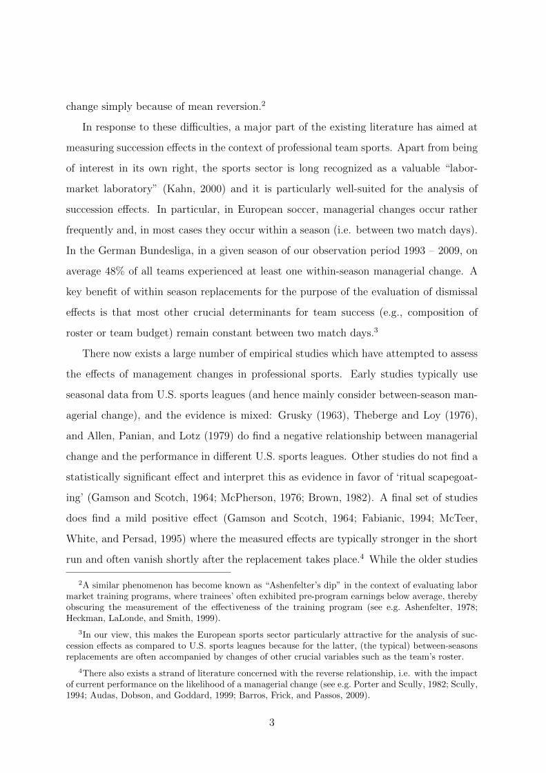
Finally, panel (a) of Figure 4 shows the average of the number of points won in the six
games before and after dismissal for all teams with a within-season dismissal, suggesting
a negative trend in performance as a key source of managerial change which points at the
importance of controlling for the exact short-term sequence of performance to exclude
hand, the degree of within-team competition may be larger in homogenous teams. But on the otherhand, the quality of the players at the lower ranks is more similar to those in the starting line-up sothat, on a competitive labor market, the same must be true for their salaries. With a given budget,a more homogenous team will then be naturally associated with a lower average player quality in thestarting line-up.
15

20
25
30
frequency ofdismissals
0
5
10
15
20
25
30
1st - 6th 7th - 12th 13th - 17th 18th - 23rd 24th - 29th 30th - 34th
frequency ofdismissals
Match Day
(a) Across Match Days
121416182022
frequency ofdismissals
02468
10121416182022
2 3 4 5 6 7 8 9 10 11 12 13 14 15 16 17 18
frequency ofdismissals
League Position
(b) Across League Positions
Figure 3: Distribution of Dismissals
mean reversion as a driver of the observed performance increase.
0
0.2
0.4
0.6
0.8
1
1.2
1.4
1.6
t-6 t-5 t-4 t-3 t-2 t-1 t+1 t+2 t+3 t+4 t+5 t+6
average points
per game
before dismissal after dismissal
(a) All Teams
0
0.2
0.4
0.6
0.8
1
1.2
1.4
1.6
1.8
t-6 t-5 t-4 t-3 t-2 t-1 t+1 t+2 t+3 t+4 t+5 t+6
hom hetaverage points
per game
before dismissal after dismissal
(b) Homogenous Versus Heterogenous Teams
Figure 4: Team Performance Before and After Dismissal
Importantly, our key hypothesis that positive succession effects emerge in homogenous
rather than heterogenous teams, should not be driven by mean reversion. Rather, as
argued by Hoffler and Sliwka (2003), managerial change should be more successful in
homogenous teams where it is easier for the new manager to re-vive the competition
for the available slots as players are operating in a now more competitive environment.
In contrast, when there is a large difference in abilities between the top players in the
team and the rest, a new manager will basically have to pick the same starting line-up
as his predecessor so that within-team competition cannot be triggered anew through a
dismissal.
As a first step in assessing the validity of our main hypothesis, panel (b) of Figure
16
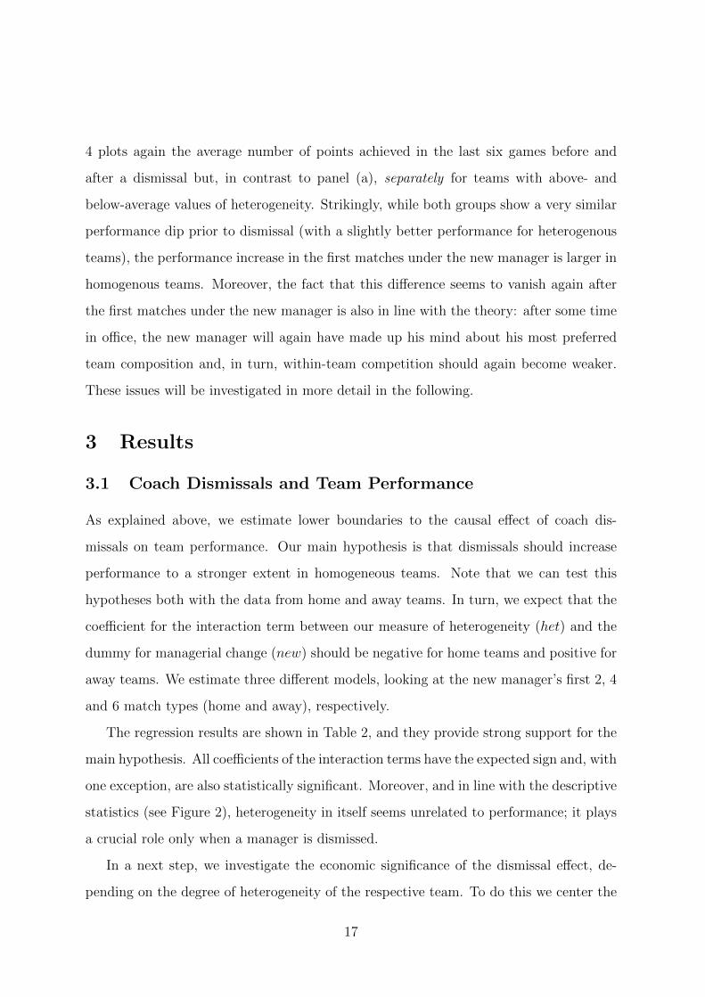
4 plots again the average number of points achieved in the last six games before and
after a dismissal but, in contrast to panel (a), separately for teams with above- and
below-average values of heterogeneity. Strikingly, while both groups show a very similar
performance dip prior to dismissal (with a slightly better performance for heterogenous
teams), the performance increase in the first matches under the new manager is larger in
homogenous teams. Moreover, the fact that this difference seems to vanish again after
the first matches under the new manager is also in line with the theory: after some time
in office, the new manager will again have made up his mind about his most preferred
team composition and, in turn, within-team competition should again become weaker.
These issues will be investigated in more detail in the following.
3 Results
3.1 Coach Dismissals and Team Performance
As explained above, we estimate lower boundaries to the causal effect of coach dis-
missals on team performance. Our main hypothesis is that dismissals should increase
performance to a stronger extent in homogeneous teams. Note that we can test this
hypotheses both with the data from home and away teams. In turn, we expect that the
coefficient for the interaction term between our measure of heterogeneity (het) and the
dummy for managerial change (new) should be negative for home teams and positive for
away teams. We estimate three different models, looking at the new manager’s first 2, 4
and 6 match types (home and away), respectively.
The regression results are shown in Table 2, and they provide strong support for the
main hypothesis. All coefficients of the interaction terms have the expected sign and, with
one exception, are also statistically significant. Moreover, and in line with the descriptive
statistics (see Figure 2), heterogeneity in itself seems unrelated to performance; it plays
a crucial role only when a manager is dismissed.
In a next step, we investigate the economic significance of the dismissal effect, de-
pending on the degree of heterogeneity of the respective team. To do this we center the
17

Model 1 Model 2 Model 3
short-term intermediate-term long-term(τ = 2) (τ = 4) (τ = 6)
New home 0.4823* 0.4319** 0.4349**(0.2757) (0.2106) (0.1806)
New home * het home -0.4853* -0.4532** -0.4316**(0.2562) (0.2004) (0.1725)
het home 0.0848 0.0852 0.0887(0.0606) (0.0620) (0.0629)
New away -0.7359*** -0.4239** -0.3988**(0.2627) (0.2097) (0.1787)
New away * het away 0.6518*** 0.3064 0.3582**(0.2523) (0.2017) (0.1717)
het away -0.0553 -0.0562 -0.0686(0.0590) (0.0604) (0.0617)
HomePerf home 0.1451*** 0.1434*** 0.1463***(0.0433) (0.0437) (0.0440)
AwayPerf home 0.1225*** 0.1179*** 0.1169***(0.0390) (0.0393) (0.0395)
HomePerf away -0.1246*** -0.1267*** -0.1235***(0.0375) (0.0379) (0.0382)
AwayPerf away -0.1788*** -0.1880*** -0.1836***(0.0447) (0.0450) (0.0454)
Perf hist home -0.0050 -0.0052 -0.0050(0.0036) (0.0036) (0.0036)
Perf hist away 0.0096*** 0.0093*** 0.0097***(0.0035) (0.0035) (0.0035)
Budget home 0.2745*** 0.2736*** 0.2766***(0.0683) (0.0683) (0.0682)
Budget away -0.2303*** -0.2272*** -0.2276***(0.0703) (0.0703) (0.0704)
Crucial home 0.0790* 0.0832* 0.0802*(0.0454) (0.0454) (0.0456)
Crucial away -0.0138 -0.0089 -0.0106(0.0457) (0.0458) (0.0459)
Past Perf Dummies home yes yes yes
Past Perf Dummies away yes yes yes
Season Dummies yes yes yes
Constant 1.8639*** 1.9163*** 1.7176***(0.5144) (0.5157) (0.4521)
Observations 4263 4259 4255Adjusted R-squared 0.080 0.081 0.081
Dependent variable: Number of points won by the home team (Result).
(Robust) Standard errors in parentheses. * p<0.1, ** p<0.05, *** p<0.01
Table 2: Managerial Change and Team Heterogeneity
18
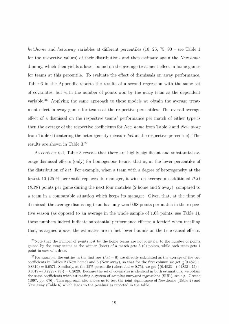
het home and het away variables at different percentiles (10, 25, 75, 90 – see Table 1
for the respective values) of their distributions and then estimate again the New home
dummy, which then yields a lower bound on the average treatment effect in home games
for teams at this percentile. To evaluate the effect of dismissals on away performance,
Table 6 in the Appendix reports the results of a second regression with the same set
of covariates, but with the number of points won by the away team as the dependent
variable.26 Applying the same approach to these models we obtain the average treat-
ment effect in away games for teams at the respective percentiles. The overall average
effect of a dismissal on the respective teams’ performance per match of either type is
then the average of the respective coefficients for New home from Table 2 and New away
from Table 6 (centering the heterogeneity measure het at the respective percentile). The
results are shown in Table 3.27
As conjectured, Table 3 reveals that there are highly significant and substantial av-
erage dismissal effects (only) for homogenous teams, that is, at the lower percentiles of
the distribution of het. For example, when a team with a degree of heterogeneity at the
lowest 10 (25)% percentile replaces its manager, it wins on average an additional 0.31
(0.20 ) points per game during the next four matches (2 home and 2 away), compared to
a team in a comparable situation which keeps its manager. Given that, at the time of
dismissal, the average dismissing team has only won 0.98 points per match in the respec-
tive season (as opposed to an average in the whole sample of 1.68 points, see Table 1),
these numbers indeed indicate substantial performance effects; a fortiori when recalling
that, as argued above, the estimates are in fact lower bounds on the true causal effects.
26Note that the number of points lost by the home teams are not identical to the number of pointsgained by the away teams as the winner (loser) of a match gets 3 (0) points, while each team gets 1point in case of a draw.
27For example, the entries in the first row (het = 0) are directly calculated as the average of the twocoefficients in Tables 2 (New home) and 6 (New away), so that for the first column we get 1
2 (0.4823 +0.8319) = 0.6571. Similarly, at the 25% percentile (where het = 0.75), we get 1
2 (0.4823− (.04853 · .75) +0.8319−(0.7228 · .75)) = 0.2029. Because the set of covariates is identical in both estimations, we obtainthe same coefficients when estimating a system of seeming unrelated regressions (SUR), see e.g., Greene(1997, pp. 676). This approach also allows us to test the joint significance of New home (Table 2) andNew away (Table 6) which leads to the p-values as reported in the table.
19

Model H1 Model H2 Model H3
short-term intermediate-term long-term(2τ = 4) (2τ = 8) (2τ = 12)
New 0.6571*** 0.4681*** 0.4591***(het = 0) (0.0003) (0.0008) (0.0001)
New 0.3105*** 0.2285*** 0.2105***(het = 10% percentile) (0.0014) (0.0017) (0.0008)
New 0.2029*** 0.1541*** 0.1333***(het = 25% percentile) (0.0086) (0.0077) (0.0080)
New 0.0531 0.0506 0.0258(het = mean) (0.4080) (0.3076) (0.5580)
New -0.0838 -0.0441 -0.0724(het = 75% percentile) (0.2548) (0.4588) (0.1690)
New -0.2232** -0.1404* -0.1724**(het = 90% percentile) (0.0234) (0.0815) (0.0143)
New is calculated as the average of the respective coefficient(s) involving
New home in Table 2 and New away in Table 6.
The p-values (in parentheses) are based on robust standard errors and estimated
based on SUR regressions (Stata command suest).
Table 3: Average impact of managerial change on team performance at different per-centiles of heterogeneity.
Moreover, and again in line with the descriptive observation (see panel (b) of Figure
4), the “new broom effect” becomes smaller as the time horizon considered for the new
manager (τ) increases. Again, this is consistent with the idea that new manager’s ability
to trigger within-team competition anew is strongest in the first few matches of his new
team.
Last, but not least, disentangling this overall average effect of a dismissal into home
and away performance reveals that it is mainly driven by performance increases in away
games. One interpretation for this result is that in home games the players’ motivation
is substantially higher in any case because of the monitoring, support or even pressure
from the team’s own fans (recall that home team wins occur twice as often as away wins
and draws). Hence, the additional motivational push from intra-team competition from
a coach replacement in a homogenous team seems to be stronger in away games where
these other motivational mechanisms are weaker.
20

3.2 Coach Dismissals and Individual Players’ Performance
Apart from the performance impact of managerial succession on the (aggregate) team
level, an alternative route is to directly consider the (individual) player level and see
whether there is any measurable direct impact on the players’ grades. Consistent with
our underlying mechanism based on within-team competition, we would expect a stronger
response of players in the “contested” ranks. i.e. those close to rank 11 which are the
weakest players on the team or the strongest on the bench, but a weak response among
the top players as they will most certainly also be part of the starting line up under
a new coach. Moreover, as for the impact of team heterogeneity, this effect should be
stronger in more homogenous teams.
In this respect, Figure 5 plots the changes of grades for the players at the different
performance ranks (again using the average grades obtained so far) in response to dis-
missals. Panel (a) shows the change of (average) grades between the first 4 matches
under the new manager and all previous matches (in a given season) under the old one,
while panel (b) extends the time horizon to cover all matches under new manager until
the end of the season. First note that the changes are increasing in a player’s rank at
the time of dismissal and are negative at the top ranks and positive at the lower ranks.
This phenomenon is naturally explained by mean reversion of players who received top
grades in the past have less scope to improve and vice-versa those at rather lower ranks
have more scope for improvements. But the important observation here is that these
differences are bigger in homogenous teams, in particular for those players in the con-
tested ranks starting with rank 8. Moreover, from panel (b) and in line with our previous
finding, we observe that the “new broom effect” seems to disappear after the tenure of
the new manager increases.
To investigate this issue in more detail we estimated the performance change of
individual players around a coach dismissal. We first constructed a data set containing
all players of teams in which a coach has been replaced within a season. The dependent
variable is the difference between the average grade in first 4 matches under new manager
21

-0.6
-0.4
-0.2
0
0.2
0.4
0.6
0.8
1 2 3 4 5 6 7 8 9 10 11 12 13 14 15 16 17 18
homogenous
heterogenous
rank ofplayerbefore
dismissal
(average grade of player in 1st - 4th match after dismissal) -(average grade of player before dismissal)
(a) First 4 Matches
-0.6
-0.4
-0.2
0
0.2
0.4
0.6
0.8
1 2 3 4 5 6 7 8 9 10 11 12 13 14 15 16 17 18
homogenous
heterogenous
rank of player before
dismissal
(average grade of player after dismissal) - (average grade of player before dismissal)
(b) All Matches
Figure 5: Change in Player Performance after Dismissal
and that in all matches (in a given season) under old one. The key independent variables
are a dummy indicating whether the team’s homogeneity is above average as well as the
player’s rank prior to the dismissal. The key hypotheses is that grade improvements due
to coach replacements are stronger (i) in more homogenous teams and (ii) for players of
lower ranks.
Model 4 Model 5
Homogenous Dummy 0.2500*** 0.0904(0.0736) (0.1015)
Rank of player (before dismissal) 0.0499*** 0.0415***(0.0048) (0.0059)
Homogenous * Rank 0.0150*(0.0085)
Shape 0.2387** 0.2398**(0.0986) (0.0994)
Budget 0.0621 0.0582(0.1080) (0.1082)
Perf hist -0.0089 -0.0090(0.0070) (0.0070)
PointsAvg (current season) -0.4711*** -0.4753***(0.1748) (0.1756)
Position Dummies yes yes
Year Dummies yes yes
Constant -0.4018 -0.3091(0.2488) (0.2538)
Observations 1771 1771Adjusted R-squared 0.103 0.105
Dependent variable: Difference (average) grade in first 4 matches under
new manager and all matches (in a given season) under the old one.
(Robust) Standard errors in parentheses.
* p<0.1, ** p<0.05, *** p<0.01
Table 4: Impact of Dismissals on Individual Performance
22

The regression results (with standard errors clustered on each separate coach dis-
missal) are shown in Table 4, and they confirm these hypotheses: As can be seen from
the first column, the change in player performance as a result of managerial change is on
average stronger for homogenous teams and for players at lower ranks (at the time of dis-
missal). More importantly, in the second column, we include an interaction term between
team homogeneity and performance rank. This term is positive, thereby supporting the
hypothesis that the change in performance at the more contested lower ranks is stronger
for homogenous teams. Hence, managerial change seems most effective in this segment
of the roster and for homogenous teams, as there the effect of better performance due
to increased within-team competition is strongest. Note that these effects cannot driven
by mean reversion, as in homogenous teams the players at these ranks tend to perform
better prior to a replacement (see Figure 2), which makes it harder for them to attain
further performance increases.
3.3 The Impact of Team Heterogeneity Under Interim Man-
agers
Recall that we have excluded interim managers from the main analysis, because their
spell was usually very short (on average a mere 2.3 matches) and, more importantly,
they are typically known to be interim solutions, only responsible for the team until
the arrival of the “real” replacement for the old manager and mostly they have worked
for the same club before – typically as an assistant to the outgoing coach. Given their
very short tenure as responsible coach and given that they are typically well acquainted
with the players, our theory based on within-team competition would predict that new
interim managers are less successful in triggering within-competition anew compared to
those new managers who are hired from the outside and expected to stay for longer.28 As
a result, and in contrast to our main findings as reported in Table 2, we should expect to
see no sizeable effect of team heterogeneity on team performance when an interim coach
takes over. Table 5 shows the results of the same regressions as above with an additional
28We are grateful to Loek Groot for this suggestion.
23

dummy indicating whether or not the new manager is an interim coach. Indeed, the
interaction terms are not significant for interim managers so that, in contrast to their
more permanent counterparts, there is no effect with respect to team heterogeneity.
4 Conclusion
The allocation of tasks to subordinates is a core management responsibility not only
in sports but nearly any kind of organization. When subordinates have preferences on
tasks of different importance, subordinates compete for the most important tasks that
for instance may help to advance their careers. And this competition can be a powerful
incentive mechanism. However, it will crucially depend upon the manager’s allocation
choices. As shown by Hoffler and Sliwka (2003), a manager who knows his subordinates
very well will assign the most important tasks to the subordinate she perceives to be the
most able. However, when this is transparent, competition among the subordinates will
be rather weak as their roles are more or less fixed. In such a situation, dismissing the
manager may trigger the competition for attractive tasks anew. A new manager who
does not know the talents of her subordinates as precisely as her predecessor will have to
make up her mind on the subordinates’ talents. In turn the subordinates have a strong
incentive to exert effort to convince the new manager of their abilities. We have explored
this mechanism empirically in professional sports, a field where it should be of substantial
importance as picking a subset of players from a larger team is a core management task
of any coach. Our key hypothesis was that coach replacements have a stronger effect on
team performance in more homogenous teams compared to heterogenous ones. Indeed
we found that coach replacements are beneficial when the abilities of the weakest players
just on the team and the strongest ones on the bench are similar.
This result has direct implications for the decision to replace coaches in professional
sports. It is notable that in many sports, it is used as a key mechanism to boost perfor-
mance in the short run, for instance to avoid relegation or to qualify for the prestigous
UEFA leagues. As laid out above, in the German Bundesliga, one of the biggest football
24

Model 7 Model 8 Model 9
short-term intermediate-term long-term(τ = 1) (τ = 2) (τ = 3)
New home 0.8387** 0.4648* 0.4236*(0.3586) (0.2754) (0.2354)
New home * het home -0.8277** -0.4680* -0.4022*(0.3241) (0.2556) (0.2243)
het home 0.0704 0.0787 0.0845(0.0595) (0.0603) (0.0610)
Interim home -1.5092 -0.6349 -0.5696(1.2677) (1.1302) (1.1339)
Interim home * het home 1.4830 0.6239 0.4996(1.0410) (0.9497) (0.9567)
New away -0.9405*** -0.7395*** -0.4906**(0.3411) (0.2623) (0.2348)
New away * het away 0.8664*** 0.6611*** 0.3976*(0.3247) (0.2518) (0.2262)
het away -0.0461 -0.0634 -0.0620(0.0581) (0.0590) (0.0596)
Interim away 0.8522 0.8248 0.8320(1.0809) (0.8037) (0.8018)
Interim away * het away -0.8018 -0.4732 -0.4824(0.8737) (0.6685) (0.6667)
HomePerf home 0.1433*** 0.1450*** 0.1458***(0.0428) (0.0430) (0.0433)
AwayPerf home 0.1289*** 0.1292*** 0.1285***(0.0387) (0.0388) (0.0390)
HomePerf away -0.1214*** -0.1199*** -0.1199***(0.0373) (0.0374) (0.0376)
AwayPerf away -0.1708*** -0.1716*** -0.1755***(0.0443) (0.0444) (0.0446)
Perf hist home -0.0054 -0.0056 -0.0056(0.0035) (0.0035) (0.0036)
Perf hist away 0.0106*** 0.0106*** 0.0103***(0.0035) (0.0035) (0.0035)
Budget home 0.2645*** 0.2655*** 0.2624***(0.0677) (0.0677) (0.0677)
Budget away -0.2158*** -0.2181*** -0.2178***(0.0702) (0.0700) (0.0700)
Crucial home 0.0754* 0.0775* 0.0774*(0.0453) (0.0453) (0.0454)
Crucial away -0.0069 -0.0074 -0.0061(0.0454) (0.0455) (0.0455)
Past Perf Dummies home yes yes yes
Past Perf Dummies away yes yes yes
Season Dummies yes yes yes
Constant 1.6625*** 1.8840*** 1.4546***(0.4780) (0.4413) (0.4752)
Observations 4320 4318 4316Adjusted R-squared 0.079 0.079 0.078
Dependent variable: Number of points won by the home team (Result).(Robust) Standard errors in parentheses. * p<0.1, ** p<0.05, *** p<0.01
Table 5: (Interim) Managerial Change and Team Heterogeneity
25

leagues in the world and the largest in terms of the number of spectators nearly half of
the clubs dismiss a coach at some point within a season. As our results show this can
indeed be a reasonable policy – but only when within-team competition can be triggered
by a dismissal which, as we have shown, is the case only when teams are rather homoge-
nous. Hence, a simple rule of thumb implied by our results would be dismissal are more
likely to beneficial when the respective team’s players do not too differ substantially in
terms of their quality. Indeed, club executives may intuitively have grasped some of this
intuition as we find that 57% of all coach dismissals occur in teams with below average
heterogeneity at the time of the dismissal.
But the result also contains some insights for other organizations. Firms frequently
not only use dismissals, but also job rotation policies by exchanging managers across
different functions or departments, to bring in “fresh air”. Our results indicate that
this can indeed reinvigorate the incentives of subordinates. But again an important
caveat is that this mechanism only works when these subordinates are on a rather equal
footing. If this is not the case the costs of a rotation or dismissal (for instance due to a
loss in human capital or specific investments) may outweigh the gains. Our results also
give some insights for the theory of tournaments or contests. A key theoretical result
established in the literature on contests and tournaments is that competition creates the
strongest incentives when players are rather homogenous. Our observations are well in
line with this result. Moreover, the results hint at a mechanism how homogeneity can be
increased in the real world even when the set of contestants cannot be changed: replacing
the decision maker to reinvigorate the race for attractive positions by “destroying” some
information on relative performance differences.
Finally, the paper also yields some methodological insights concerning the economet-
ric evaluation of the effect of managerial change on performance. As we have pointed out,
estimates in observational studies where proper instrumental variables are unavailable
will be biased when executives who decide upon dismissals have further unobservable
private information on future states. But as we have shown this mechanism induces
a negative selection bias – and, in turn, typical regression models will underestimate
26

the true effect. Hence, the fact that previous studies have typically found no or even
negative effects does not tell us that coach dismissals are detrimental or useless. To the
contrary, as suggested by our paper they can lead to substantial performance effects in
homogenous teams.
27

Appendix
Model 1 Model 2 Model 3
short-term intermediate- long-term(τ = 2) term (τ = 4) (τ = 6)
New home -0.3368 -0.3354* -0.3017*(0.2631) (0.2011) (0.1706)
New home * het home 0.3100 0.3489* 0.2817*(0.2450) (0.1920) (0.1629)
het home -0.0443 -0.0467 -0.0426(0.0579) (0.0591) (0.0601)
New away 0.8319*** 0.5042** 0.4834***(0.2518) (0.2040) (0.1729)
New away * het away -0.7228*** -0.3818** -0.4350***(0.2318) (0.1939) (0.1644)
het away 0.0623 0.0704 0.0845(0.0566) (0.0578) (0.0592)
HomePerf home -0.1173*** -0.1144*** -0.1184***(0.0414) (0.0417) (0.0421)
AwayPerf home -0.1069*** -0.1021*** -0.1024***(0.0369) (0.0372) (0.0374)
HomePerf away 0.1014*** 0.1042*** 0.1022***(0.0356) (0.0359) (0.0362)
AwayPerf away 0.1779*** 0.1862*** 0.1825***(0.0427) (0.0430) (0.0434)
Perf hist home 0.0042 0.0044 0.0042(0.0034) (0.0034) (0.0034)
Perf hist away -0.0089*** -0.0086*** -0.0089***(0.0033) (0.0033) (0.0033)
Budget home -0.2815*** -0.2811*** -0.2833***(0.0639) (0.0640) (0.0638)
Budget away 0.2304*** 0.2282*** 0.2283***(0.0682) (0.0683) (0.0683)
Crucial home -0.0660 -0.0702 -0.0670(0.0431) (0.0432) (0.0433)
Crucial away 0.0262 0.0214 0.0230(0.0437) (0.0438) (0.0439)
Past Perf Dummies home yes yes yes
Past Perf Dummies away yes yes yes
Season Dummies yes yes yes
Constant 0.8920* 0.8349* 1.0371**(0.5032) (0.5043) (0.4312)
Observations 4263 4259 4255Adjusted R-squared 0.076 0.076 0.076
Dependent variable: Number of points won by the away team.(Robust) Standard errors in parentheses. * p<0.1, ** p<0.05, *** p<0.01
Table 6: Impact of Managerial Change and Team Heterogeneity in Away Games
28

References
Allen, M., S. Panian, and R. Lotz (1979): “Managerial succession and organiza-
tional performance: A recalcitrant problem revisited,” Administrative Science Quar-
terly, 24(2), 167–180.
Angrist, J., and J. Pischke (2008): Mostly harmless econometrics: An empiricist’s
companion. Princeton University Press.
Ashenfelter, O. (1978): “Estimating the effect of training programs on earnings,”
The Review of Economics and Statistics, 60(1), 47–57.
Audas, R., S. Dobson, and J. Goddard (1999): “Organizational Performance and
Managerial Turnover,” Managerial and Decision Economics, 20, 305–318.
(2002): “The impact of managerial change on team performance in professional
sports,” Journal of Economics and Business, 54(6), 633–650.
Audas, R., J. Goddard, and S. Dobson (1997): “Team Performance and Managerial
Change in the English Football League,” Economic Affairs, 17(3), 30–36.
Baik, K. (1994): “Effort Levels in Contests with Two Asymmetric Players.,” Southern
Economic Journal, 61(2).
Barros, C., B. Frick, and J. Passos (2009): “Coaching for survival: the hazards
of head coach careers in the German ‘Bundesliga’,” Applied Economics, 41(25), 3303–
3311.
Berger, J., and P. Nieken (2010): “Heterogeneous Contestants and Effort Pro-
vision in Tournaments - An Empirical Investigation with Professional Sports Data,
mimeographed,” University of Bonn, SFB/TR 15 Discussion Paper No. 325.
Brown, J. (2011): “Quitters never win: The (adverse) incentive effects of competing
with superstars,” Journal of Political Economy, 119(5), 982–1013.
29

Brown, M. (1982): “Administrative succession and organizational performance: The
succession effect,” Administrative Science Quarterly, 27(1), 1–16.
Bruinshoofd, A., and B. ter Weel (2003): “Manager to go? Performance dips
reconsidered with evidence from Dutch football,” European Journal of Operational
Research, 148(2), 233–246.
Clark, D. J., and C. Riis (2000): “Allocation Efficiency in a Competitive Bribery
Game,” Journal of Economic Behavior & Organization, 42, 109–124.
de Dios Tena, J., and D. Forrest (2007): “Within-season dismissal of football
coaches: Statistical analysis of causes and consequences,” European Journal of Oper-
ational Research, 181(1), 362–373.
De Paola, M., and V. Scoppa (2012): “The effects of managerial turnover: evidence
from coach dismissals in Italian soccer teams,” Journal of Sports Economics, 13(2),
152–168.
Fabianic, D. (1994): “Managerial Change and Organizational Effectiveness in Major
League Baseball: Findings for the Eighties.,” Journal of Sport Behavior, 17(3), 139–
152.
Feess, E., G. Muehlheusser, and M. Walzl (2008): “Unfair Contests,” Journal
of Economics, 93(3), 267–291.
Fullerton, R., and R. P. McAfee (1999): “Auctioning Entry into Tournaments,”
Journal of Political Economy, 107, 573–605.
Gamson, W., and N. Scotch (1964): “Scapegoating in Baseball,” American Journal
of Sociology, 70(1), 69–72.
Gradstein, M. (1995): “Intensity of competition, entry and entry deterrence in rent
seeking contests,” Economics & Politics, 7(1), 79–91.
Greene, W. H. (1997): Econometric analysis. Prentice Hall, Upper Saddle River.
30

Grusky, O. (1963): “Managerial Succession and Organizational Effectiveness,” Amer-
ican Journal of Sociology, 69(1), 21–31.
Heckman, J., R. LaLonde, and J. Smith (1999): “The economics and econometrics
of active labor market programs,” Handbook of Labor Economics, 3, 1865–2097.
Hoffler, F., and D. Sliwka (2003): “Do new brooms sweep clean? When and why
dismissing a manager increases the subordinates´ performance,” European Economic
Review, 47(5), 877–890.
Kahn, L. (2000): “The Sports Business as a Labor Market Laboratory,” Journal of
Economic Perspectives, 14(3), 75–94.
Lazear, E., and S. Rosen (1981): “Rank-Order Tournaments as Optimum Labor
Contracts,” Journal of Political Economy, 89(5), 841–864.
Lien, D. D. (1990): “Corruption and Allocation Efficiency,” Journal of Development
Economics, 33, 153–164.
Lynch, J. (2005): “The effort effects of prizes in the second half of tournaments,”
Journal of Economic Behavior and Organization, 57(1), 115–129.
McPherson, B. (1976): “Involuntary Turnover: A Characteristic Process of Sport
Organizations,” International Review for the Sociology of Sport, 11(4), 5–16.
McTeer, W., P. White, and S. Persad (1995): “Manager Coach Mid-Season Re-
placement and Team Performance in Professional Team Sport.,” Journal of Sport
Behavior, 18(1), 58–68.
Moldovanu, B., and A. Sela (2006): “Contest Architecture,” Journal of Economic
Theory, 126(1), 70–97.
Nalebuff, B., and J. Stiglitz (1983): “Prizes and incentives: towards a general
theory of compensation and competition,” The Bell Journal of Economics, pp. 21–43.
31

Nickell, S. (1981): “Biases in dynamic models with fixed effects,” Econometrica, 49(6),
1417–1426.
Nieken, P., and M. Stegh (2010): “Incentive Effects in Asymmetric Tournaments
Empirical Evidence from the German Hockey League,” University of Bonn, SFB/TR
15 Discussion Paper No .305.
Nti, K. (1999): “Rent-seeking with asymmetric valuations,” Public Choice, 98(3), 415–
430.
O’Keeffe, M., W. Viscusi, and R. Zeckhauser (1984): “Economic contests: Com-
parative reward schemes,” Journal of Labor Economics, 2(1), 27–56.
Orrison, A., A. Schotter, and K. Weigelt (2004): “Multiperson tournaments:
An experimental examination,” Management Science, 50, 268–279.
Porter, P., and G. Scully (1982): “Measuring managerial efficiency: the case of
baseball,” Southern Economic Journal, 48(3), 542–550.
Rowe, W., A. Cannella, D. Rankin, and D. Gorman (2005): “Leader succession
and organizational performance: Integrating the common-sense, ritual scapegoating,
and vicious-circle succession theories,” The Leadership Quarterly, 16(2), 197–219.
Schotter, A., and K. Weigelt (1992): “Asymmetric tournaments, equal opportu-
nity laws, and affirmative action: Some experimental results,” The Quarterly Journal
of Economics, 107(2), 511–539.
Scully, G. (1994): “Managerial efficiency and survivability in professional team
sports,” Managerial and Decision Economics, 15(5), 403–411.
Sunde, U. (2009): “Heterogeneity and performance in tournaments: a test for incentive
effects using professional tennis data,” Applied Economics, 41(25), 3199–3208.
Szymanski, S., and T. Valletti (2005): “Incentive effects of second prizes,” European
Journal of Political Economy, 21(2), 467–481.
32

Taylor, C. (1995): “Digging for Golden Carrots: an Analysis of Research Tourna-
ments,” American Economic Review, 85(4), 872–890.
Theberge, N., and J. Loy (1976): “Replacement Processes in Sport Organizations:
the Case of Professional Baseball,” International Review for the Sociology of Sport,
11(2), 73–93.
33