Embed Size (px)
Citation preview

The Impact of Living Wage Ordinances on Urban Crime
Jose Fernandez Department of Economics University of Louisville
Thomas Holman San Francisco, California
John V. Pepper Department of Economics
University of Virginia [email protected]
July 5, 2013 JEL CODES: I18, H73, R50 ABSTRACT: We examine the impact of living wages on crime. Past research has found that living wages appear to increase unemployment while providing greater returns to market work. The impact on crime, therefore, is unclear. Using data on annual crime rates for large cities in the United States, we find that living wage ordinances are associated with notable reductions in property related crime and no discernable impact on non-property crimes. Acknowledgement: We thank Scott Adams for providing data on living wage ordinances through 2002. Parts of the crime data used in this paper were assembled by Rob Fornango, and made available to the authors by the Committee on Law and Justice. The authors remain solely responsible for how the data have been used and interpreted. Pepper’s research was supported in part by the Bankard Fund for Political Economy.

1
I. Introduction
Over the past 15 years, a number of city governments have adopted living wage
ordinances mandating wage floors exceeding the federal minimum wage for certain
classes of workers. These floors have been found to impact the labor market for low
skilled workers, leading to fairly substantial increases in expected wages and a small but
statistically significant reduction in employment (Neumark and Adams, 2003b;
Campolieti, Fang, and Gunderson, 2005). To the extent that these wage floors impact the
labor market of the low-skilled, they might also affect non-labor market behaviors such
as crime. In this paper, we examine the unintended impact of living wage ordinances on
crime.
In the standard neo-classical model, the opportunity cost of working in the legal
sector may influence the propensity to commit crime (Becker, 1968; Levitt, 1997). These
ideas, in fact, are supported in the existing empirical literature which reveals a modest
effect of unemployment and a somewhat more pronounced and lasting effect of wages on
pecuniary crimes (see, for examples, Grogger, 1998; Freeman, 1999; Gould et al., 2002;
Lin, 2008). This model, however, does not lead to a qualitative prediction about the
impact of wage floors on crime. Rather, by simultaneously increasing the returns to
employment and the likelihood of unemployment, theoretical predictions about the
impact of living wage ordinances on crime are ambiguous. An increase in wages among
the working low skilled might be expected to decrease crime, yet the associated decrease
in employment might lead to an increase in crime. Given that living wage ordinances are
found to have only a small negative impact on employment but a much more pronounced
positive effect on wages, one might reasonably speculate these ordinances lead to a

2
reduction in crime. Ultimately, however, this is an empirical question which has not yet
been addressed in the literature.
To resolve this ambiguity, we use panel data on annual city level crime rates and
living wage ordinances from 1990-2010. For each city-year, we observe the rates of
different types of property and violent crimes, the minimum and the living wage, and a
detailed set of covariates. Given these data, the basic empirical approach compares crime
rates in cities before and after the adoption of living wage laws, as well as crime rates
between cities that did and did not adopt living wage ordinances.
As with all such studies, a primary concern is that living wage ordinances may not
be exogenous; living wages may be adopted or changed in response to factors that are
unobserved to the econometrician but are arguably associated with crime. For example,
local labor market conditions, the fiscal stability of local governments, and social services
provided by local governments may all be associated with living wage provisions and
crime.
To account for the nonrandom adoption of living wage laws, we use several
nested approaches. First, at the most basic level, we estimate models with a rich set of
covariates accounting for city/county and state level socio-economic and criminal justice
variables that might confound inferences. Likewise, we exploit the panel nature of the
data by incorporating both city and time fixed effects, city specific linear and quadratic
time trends, and state-by-year fixed effects.1 Second, in addition to presenting results for
the full sample of cities, we also restrict the analysis to cities that had a formal living
wage campaign, some of which passed and others of which did not. Arguably, this sub-
sample provides a more credible although smaller comparison group for the analysis

3
(Adams and Neumark, 2005a). Third, we employ falsification tests by examining the
impact of living wage laws on violent crime rates – most notably, the murder, assault, and
rape rates -- that seem unlikely to be notably impacted by these wage ordinances. Finally
to rule out the possibility that our results are spuriously driven by serial correlation, we
use a placebo test that regresses the crime rate on a “fake” living wage ordinance variable
that precedes the true adoption date by two years.
After describing the data in Section II, we evaluate the effects of living wage laws
on crime rates in Section III. In Section IV, we draw conclusions. Using data on annual
crime rates for large cities in the United States, we find that living wage ordinances are
associated with notable reductions in property related crime and little impact on non-
property crimes such as murder, assault and rape.
II. Data Description
The data are a panel of annual crime rates and living wage ordinances for the 239
largest U. S. cities (approximately all cities with greater than 100,000 persons) over the
period 1990 to 2010.2 Of the 239 cities included in the sample, 49 had successful living
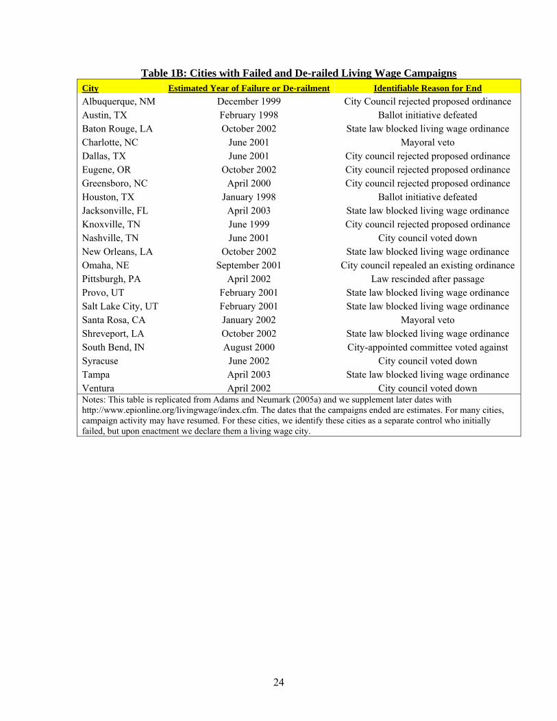
wage campaigns and 20 had unsuccessful campaigns. Table 1A lists the 49 cities with
living wage ordinances, along with the 2010 living and minimum wages, and Table 1B
lists the cities with unsuccessful campaigns.
Several important features of living wage ordinances are revealed. First, the living
wage can be substantially higher than the minimum wage. Seventeen of the 49 cities have
living wages that exceed $13 per hour, and four cities – Berkeley, Hartford, St. Louis,
and San Jose– have living wages of $14 per hour or more. Second, many cities – 53
percent – have state minimum wages in excess of the federal floor. Nearly 47 percent of

4
cities with living wage ordinances are located in states that have minimum wages in
excess of the federal floor. Thus, it is important for us to control for the state minimum
wage. Finally, in contrast to the minimum wage, living wage ordinances only cover
limited groups of workers; those that are municipal employees, contract workers, or
workers in businesses receiving assistance from the state.3
For each city-year, we observe the living wage, if it exists, and the rates of six
different types of crimes as measured by the Federal Bureau of Investigations Uniform
Crime Reports (UCR).4 In particular, we observe rates of burglary, larceny, and motor
vehicle theft (MVT) as well as the four violent crime rates for murder, assault, rape, and
robbery. In addition, we observe a rich set of covariates measuring both socio-economic,
demographic and criminal justice variables that are typically used in crime regression
models. 5
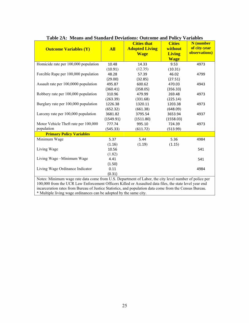
Table 2 displays basic descriptive statistics for the variables used in the analysis.
The first column of sample statistics provides means and standard deviations for all cities
across all years, while the next two columns display the sample means for cities that
adopted living wage ordinances and those that did not, respectively. Cities that adopted
living wage ordinances have larger populations and a higher fraction of minorities than
non-living wage cities (see Table 2B). In addition, living wage cities have higher crime
rates: the average homicide rate in cities adopting a living wage ordinance is 14.33 (per
100,000) whereas the analogous rate for other cities is 9.53.
Additional insight on the association between living wage ordinances and crime is
found by tracing out the temporal path of crime rates around the years when ordinances
are adopted. Figure 1 displays the time series variation in the difference between the

5
percent change in crime rates in living wage and control cities relative to the year in
which the living wage ordinance is adopted. For example, year 0 is 1998 for Boston and
2000 for Denver (see Table 1A).6 We display the cumulative percent change in the relative crime rates for cities that
did and did not adopt living wage ordinances, using five years prior to the adoption of the living wage ordinance as the baseline.
While crime rates are consistently falling in living wage cities faster than non-living wage cities throughout, there is a significant
decrease in both violent and property crime occurring at the time of the enactment. For example, from year -5 to year -1, crime rates
fell faster in living wage cities than control cities by a rate of 1.6% each year for property crime and 0.7% for violent crime. The most
striking differences, however, occur just after living wage ordinances are adopted (i.e., year 0), when property crime rates fell 5.7%
faster in living wage cities and violent crime fell by 3.1% . After the adoption, the relative change in the property and violent crime
rates remained nearly unchanged for three years then continued to fall at the same rate as prior to the adoption of the living wage
ordinance.
Whether these differences are due, in part, to the living wage ordinances or
simply unobserved factors that confound the observed associations remain unclear. To
account for factors that are thought to be associated with both crime and living wage
rates, we include a number of covariates in the regressions. Most notably, since many
cities with living wage ordinances are located in states with minimum wage rates in
excess of the federal floor (see Table 1), we include city-year specific minimum wages in
our analysis. Likewise, we include a rich set of fixed effect and covariates measuring the
demographic characteristics of the city/county, the number of police per capita, and the
state incarceration rate (see Table 2).
III. The Effect of Living Wage Ordinances on Crime

6
To evaluate whether the observed relationships between living wages and crime
reflect the effects of living wage laws, we estimate a series of linear mean regression
models that account for observed and unobserved city specific characteristics. In Section
III.A, we outline the basic fixed effect model that explicitly accounts for unobserved city
specific factors that may be related to both crime rates and living wage policies. In
Section III.B, we present and discuss the estimates from a series of models that evaluate
the effects of living wages on crime rates, and in Section III.C we evaluate the robustness
of the results to different specifications. Finally, in Section III.D we provide a brief
discussion of the results.
A. Model
To assess the impact of living wage ordinances on crime, we evaluate two basic
models. In the first, we evaluated the impact of a living wage (LW) ordinance and in the
second we consider the specific wage floor.
Formally, we consider the linear model
Yit = t + β · ln( min
itw ) + γ *LWit + Xit+ it (1)
where Yit is the log-crime rate for city i in year t, min
itw is the higher of the applicable
state or federal minimum wage rates, and Xit is the observed vector of other city i
characteristics in year t that are thought to influence the number of crimes. Finally, LW
is a measure of the living wage ordinance. For some specifications, this is simply an
indicator of whether the city adopted an ordinance. For others, the random variable
associated with the living wage is the percentage increase of the living wage relative to
the effective minimum wage in cities with non-trivial living wage ordinances and equals

7
zero for all non-living wage cities: =max[ln( livitw )- ln( min
itw ),0]. The parameters t, , γ,
and are unobserved, with t being a year fixed effect. The primary parameter of
interest is γ.
Finally, the random variable it measures unobserved factors influencing crime
rates. The conventional assumption is that this unobserved random variable is mean zero
independent of all the covariates, E[it |minw , LW, X ] = 0, in which case living wage
laws are exogenous. Arguably, however, the unobserved factors, it, influencing crime are
related to unobserved factors associated with the city specific living and minimum wages.
For example, unobserved local labor market conditions and social programs may
influence the passage of living wage ordinances and crime, in which case the observed
correlations between living wage laws and crimes rates will be spurious.
To account for this identification problem, we allow for the expectation of the
unobserved factors to vary across city and time as follows:
E[it |minw , LW, X ]= Ci + T1it + T2it
2 + eit (2)
Equations (1) and (2) imply a mean regression that includes an identically and
independently distributed shock eit, a city fixed effect, Ci, and city specific linear and
quadratic time trends, T1it + T2it2. Thus, the model explicitly accounts for unobserved
time and city specific factors that might jointly influence living wage laws and crime
rates. The effect of the living wage is identified using within-city variation in living wage
after netting out city-specific time trends. Coupled with the rich set of covariates, this
flexible panel data specification should minimize the influence of many unobserved
confounders. Incorporating flexible city specific time trends is especially important given
8
the heterogeneous decrease in crime over time between living wage and control cities as
noted in Figure 1 as well as the well documented and dramatic fall in crime during the
1990’s (Levitt, 2004). Finally, to assess the importance of state-level unobserved
heterogeneity, we also estimate a model with state-by-year fixed effects (see Section
III.C).
We assess the sensitivity of the parameter estimates to different assumptions on
city specific parameters, Ci, T1, and T2. In each case, we use a least-squares estimator,
weighted to account for differences in city populations, to consistently estimate the
parameters, and report robust standard errors clustered by city to allow for arbitrary
heteroskedasticity.
B. Results
Table 3 presents the estimated effect of living wage ordinances on crime, where
the living wage ordinances are represented by an indicator variable. Table 3A present
results for the three property crimes and Table 3B presents results for the four violent
crimes. Using data from the entire sample of 239 cities, the table presents estimates from
five different panel data specifications: the first uses year fixed effects alone, the second
with year and city fixed effects, the third adds other time varying covariates, the fourth
adds a city specific linear time trend, and the fifth includes both city specific linear and
quadratic trends.7
The estimated effect of living wages is sensitive to whether we account for
unobserved city specific fixed effects and time trends. Model 1 estimates include year but
not city fixed effects or other covariates. Except for rape, violent crime rates are found to
be substantially higher after living wage ordinances are passed and are statistically
9
significant at the 5% level. For the three property crimes, the estimates are not
statistically significant, yet suggest large negative associations for burglary and larceny
and a positive association for MVT.
Once we account for the covariates, city fixed effects and time trends in Models
3-5, however, many of these observed associations appear spurious. Most notably, the
estimates from these fixed effects models imply that living wage ordinances decrease the
three property crimes analyzed in this study. In particular, the living wage ordinances are
estimated to reduce the burglary rate by 6% to 8%, the MVT rate by 6% to 12% and the
larceny rate by 2% to 3%. Although the larceny estimates from Models 3-5 are
statistically insignificant, the fact that the estimates are consistently negative across all
five specifications and that the Model 2 estimate of -7.2% is statistically significant
suggests that living wages do have a small negative impact on larceny.
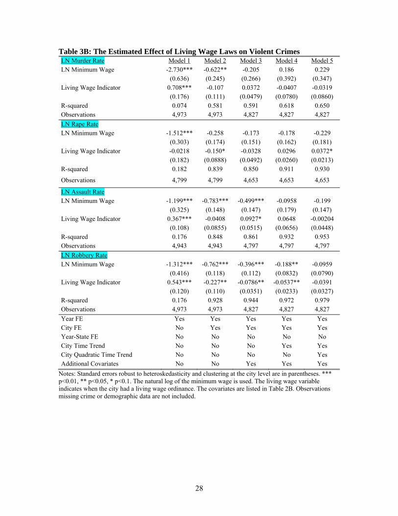
Table 3B presents analogous results for violent crimes. As might be expected,
living wage ordinances appear to have little discernable impact on murder, rape, and
assault, but do appear to reduce the robbery rate by between 4 and 8%.8
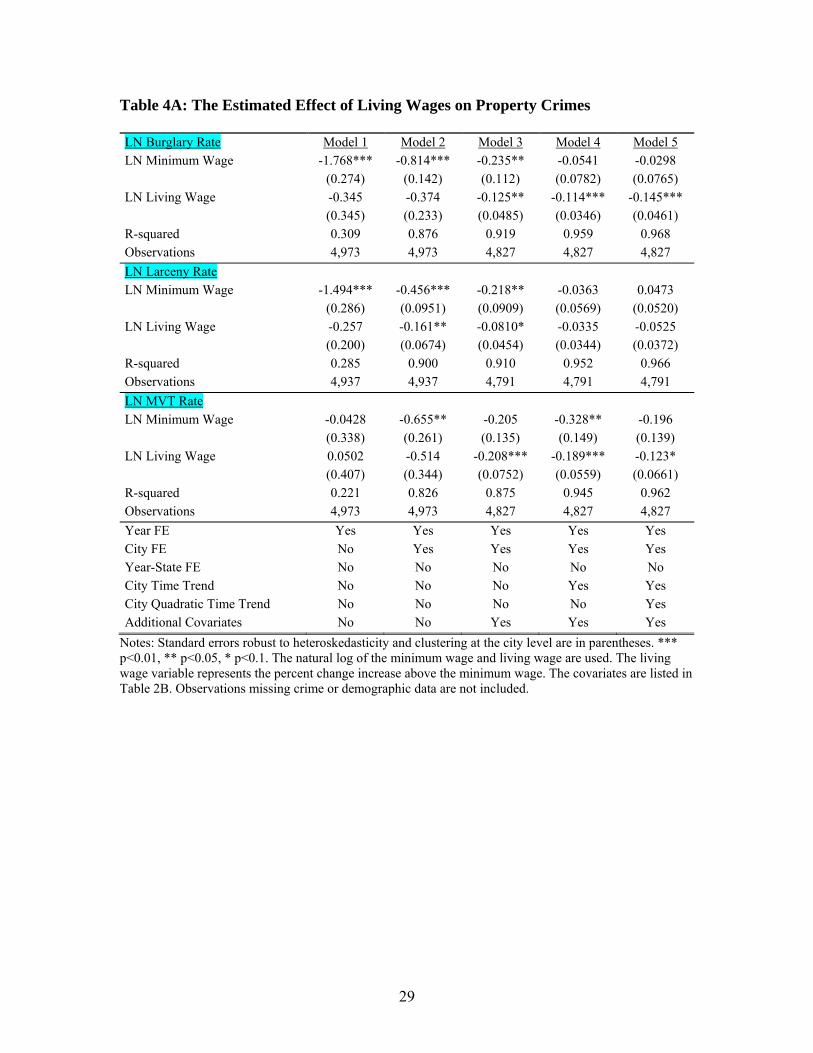
Table 4 presents estimates from models using the living wage variable directly. In
this case, the living wage coefficient estimates measure the elasticity of the living wage
on crime. In particular, holding the minimum wage constant, γ measures the elasticity of
crime rates with respect to an increase in the living wage over the effective minimum
wage. Again, we find that the living wage reduces the rates of property related crime but
not violent crime. For example, the elasticity of burglary and MVT rates with respect to
living wage are estimated to be around -0.15. In contrasts, we cannot reject the null
hypothesis that living wages have no impact on murder, rape and assault.
10
C. Robustness Analysis
To further assess the robustness of our findings, we consider three alternative
specifications. First, we restrict the analysis to cities that had a formal living wage
campaign brought before the city government, some of which passed and others of which
did not. Arguably, cities with failed living wage campaigns provide a more natural
comparison group for the analysis. Second, with multiple cities in each state, we employ
state-year fixed effects to further control for time-varying state specific confounders.
Finally, we use a placebo test in which we regress the crime rate on a “fake” living wage
ordinance variable that precedes the true adoption date by two years.
i. Failed Campaigns
Living wage campaigns have been unsuccessful in numerous cities. In our
sample, for example, 22 of the 239 cities had unsuccessful campaigns (see Table 1B).
Arguably, cities that have undergone unsuccessful campaigns provide a better control
group for estimating the effects of living wage laws than the broader set of all cities.
After all, living wage movements may be accompanied by increased attention,
organization and public debate on workers at the bottom of the wage distribution.
Narrowing the control group to those cities with living wage campaigns, may avoid
confounding the effects of living wage laws and living wage campaigns.
Thus, in this section, we re-estimate Models 4 and5 on a subset of cities that have
had living wage campaigns.9 The estimates are found in the top panel of Table 5, which
displays coefficients and standard errors using the restricted sample of 71 cities with
living wage campaigns. As we found with the full sample, the evidence suggests that
11
living wage ordinances and living wages reduce the three property crimes and robbery.
In particular, these ordinances are estimated to reduce the robbery rate by 6 to 7 percent,
the burglary rate by 7 to 9 percent, the larceny rate by 3 to 4 percent (statistically
insignificant), and the MVT rate by 6 to 10 percent. At the same time, there is no
statistically significant impact of the living wage on homicide, rape or assault.
Next, following Adams and Neumark (2005a), we consider these failed
campaigns within the full sample of cities by constructing an indicator variable marking
the initial year and subsequent years after a failed campaign (FLW). Campaigns are de-
railed or failed after a significant action by local or state government against the proposal
(e.g. mayoral veto or city council rejection).10 Using this indicator for failed campaigns,
the regression specification is modified to include these failed campaigns as a second
control group as follows:
Yit
= t
+ β · ln( minitw ) + γ *LW
it + λ *FLW
it + X
it+
it (3)
We estimate Models 4 and 5 using the modified specification and report the coefficients
in the second panel of Table 5. The estimated effects associated with the living wage
ordinance are consistent with the previous findings. Living wage ordinances are
estimated to decrease the robbery rate by 3.3 to 4.8 percent and the burglary rate by 5.5 to
7.8 percent, the larceny rate by 1.5 to 2.3 percent (statistically insignificant), and the
MVT rate by 6.1 and 11.3 percent. The estimate effects for murder, rape and assault are
all statistically insignificant.
In addition to using failed campaigns as an alternative control group, the
specification in Equation 3 provides insight on whether the estimates associated with the
living wage laws reflect the effects of the laws themselves or just the effects of living

12
wage campaigns. In particular, the coefficient associated with failed or derailed living
wage campaigns, λ, reveals the impact of the campaign, albeit ones that have failed.
While many of the estimates are large in magnitude -- exceeding 0.05 in absolute value –
they are also imprecise. Twelve of the fourteen estimates associated with failed
campaigns are statistically insignificant, suggesting that there is no discernible impact of
the campaign on crime.
Still, if these estimates associated with FLW reveal the impact of living wage
campaigns, a more refined estimate of the impact of living wage laws can be found by
differencing the estimate associated with the campaigns, λ, from the estimated effect of
the ordinance, γ (see Adams and Neumark, 2005a). Focusing on Model 5 (the Model 4
results are similar), we find the difference and difference type estimates imply that living
wage ordinances decrease the robbery rate by about 12%, the burglary rate by 13%, the
larceny rate by 7%, and the MVT rate by 2% (statistically insignificant). In contrast, we
accept the zero null hypotheses for murder, rape, and assault (the estimate for rape is
significant in Model 4).
ii. Type of Living Wage Ordinance and State-Year Fixed Effects
Neumark and Adams (2003a) distinguish between ordinances on businesses
receiving government assistance (GA) and ordinances for municipal employees or
contract workers (MC). They find that the former have larger impacts on the labor market
than the latter. See footnote 3 for further details.
We incorporate these different ordinance types into our regression specification
Yijt = β · ln( minijw ) + γ1 *GAijt + γ2 *MCijt + Xijt+ jt + ui + eijt (4)

13
where j indexes state, jt is a state-year fixed effect, ui is a city fixed effect, and eijt is the
idiosyncratic error. The state-year fixed effect specification captures unobserved non-
linear state effects that may be associated with crime rates such as changes in state law or
state funding of local police departments. The top panel of Table 6 reports the
coefficients of the general living wage indicator for the different crime rates and the
lower panel reports the coefficients for the GA and MA living wage indicators for the
different crime rates.
The general living wage ordinance is found to have a statistically significant
effect on robbery, burglary, and motor vehicle theft, but no discernible effect on murder,
rape, or assault. The living wage ordinance decreases robbery by 10 percent, burglary by
3 percent and motor vehicle theft by 5 percent. However, when we disaggregate the
living wage indicator we find a heterogeneous effect on the crime rates dependent on the
type of ordinance. We find a statistically significant negative effect for the business
assistance ordinance (GA) for both larceny and robbery, but not burglary or MVT. The
GA ordinance decreases larceny by 8.6 percent and robbery by 9 percent. The MC
ordinance is found to decrease burglary by 3.6 percent and robbery by 9 percent, but we
accept the zero null hypothesis for larceny and MVT. None of the violent crimes are
statistically significant in either specification.11
iii. Policy Placebo/Falsification Test
Finally, we conduct a falsification test using fake policy variables to assess
whether there is evidence of spurious correlations (see Bertrand, Duflo and
Mullainanthan, 2004). In particular, we create a placebo living wage indicator which
equals one two years prior to the actual date the living wage ordinance is adopted. So, if

14
a living wage ordinance passed in 1998, the placebo policy indicator will equal 1 in 1996
(and beyond), two years prior to the actual passage date. Since this date is arbitrary, the
coefficient associated with this placebo should be zero. A statistically significant estimate
would suggest that the model may be mispecified and the resulting coefficient estimates
may be biased. In particular, some of the observed decrease in property crime may be due
to unobservable factors that are correlated across time and not due to the policy
intervention.
The results of the placebo test are divided into three panels in Table 7, with each
panel displaying results which include more city specific control: the top panel includes
only city fixed effect, the middle panel includes a city specific linear time trend, and the
bottom panel includes a city specific quadratic time trend. Without time trends (panel 1),
the coefficient estimates associated with the placebo variable on living wage ordinances
are relatively small but statistically significant for assault and MVT. Once linear and
quadratic time trends are incorporated in the model, however, all of the coefficient
estimates associated with the ordinances are small and insignificant. Thus, this test does
not reveal evidence that the estimates from models with city specific time trends are
biased.
D. Discussion of Results
To summarize our primary findings, we observe that living wages have a modest
negative effect on property related crimes. The Model 5 estimated elasticities on property
crimes suggest that a 1 percentage point increase in living wage relative to the effective
minimum wage results in 0.05 to 0.15 percent drop in property related crime. Likewise,
the results found when using a simple living wage indicator variable in our most

15
restrictive Model 5 suggests that a policy that caused a roughly 50% increase in the
wages for some fraction of low wage workers is associated with a 8% reduction in
burglaries, a 6% reduction in car thefts, a 4% reduction in robberies, and a 3% reduction
in larceny. At the same time, we find that the living wage has no discernable effect on
crimes with weak pecuniary motives including murder, rape, and assault.
These findings are generally consistent with both the literature evaluating the
impact of the living wage on the low skilled labor market and the literature evaluating the
impact of the labor market on crime. The former literature finds that the living wage has a
large positive effect on average wages and a small negative effect on employment. Thus,
to the extent the living wage serves to increase the expected benefits of participating the
labor market, we would predict an associated drop in crime, especially crimes with
pecuniary motives. The latter literature finds, in fact, that the labor market for low skilled
persons has a notable impact on crimes with pecuniary motives but little effect on non-
pecuniary crimes such as rape and murder (Gould et al., 2002). Since we expect the living
wage to impact crime via the low skilled labor market, the lack of relationship between
the living wage and homicide, assault, and rape suggests that our conclusions are not due
to a spurious correlation between these ordinances and general levels of crime.
Finally, note that while these estimated elasticities are substantial they are notably
smaller than estimates found for more direct policy measures aimed at reducing crime.
The literature evaluating the impact of incarceration on property crime, for example,
reports estimated elasticities that in many cases exceed -0.50 (Levitt, 1996; Johnson and
Raphael, 2010). Likewise, the literature examining the impact of policing on property
16
related crimes tends to find point estimates of at least -0.50 (Levitt, 1997, 2002 and 2004;
and Evans and Owens, 2007).
V. Conclusion
In this paper, we evaluate the unintended consequences of living wage policies on
crime. Using a panel of annual city level crime rates from 1990 to 2010, two
contributions are made to the existing literature. First, while previous studies have
focused on the impact of living wages on the labor market, we are the first to study the
impact of living wages on related deviant behaviors. Second, using the panel data set of
cities, we are able to explicitly mitigate the potential endogeneity bias of living wage
ordinances using a variety of empirical approaches.
We find robust evidence that living wage ordinances lead to modest reductions in
expected robbery, burglary, larceny, and MVT rates, but have no impact on non-
pecuniary violent crimes such as homicide, assault, and rape. These findings are
supported in a variety of different regression models. Depending on the specification and
the crime being examined, our elasticity estimates for the three property related crimes lie
between -0.03 and -0.2.
1 Adams and Neumark in their work examining the impact of living wages on employment and earnings also consider city specific linear time trends. 2 The data contain 243 cities, but some cities are dropped either due to a lack of information regarding living wage ordinances, or missing crime or covariate data leaving a total of 239 cities. 3 There is limited information about the fraction of low-skilled workers potentially impacted by living wage laws. Neumark and Adams (2003a) estimate the fraction of workers in the bottom quartile of the wage distribution potentially covered by living wage ordinances varies from 3-6% for ordinances covering municipal employees, to 15-20% for laws that cover city contractors, and to slightly over 80% for laws that cover businesses receiving government assistance. The fraction of workers actually impacted by the different ordinances, however, will be much smaller (see, for example, Farris

17
(2005) and Tolley, Bernstein, and Lesage (1999)). For example, based on survey of city contractors in Chicago, Tolley et. al. (1999) estimate that slightly more than one-third of employees in covered businesses would be impacted by the living wage ordinance applied to contract workers. Finally, Brenner, Wicks-Lim, and Pollin (2002) find the enforcement of business assistance ordinances vary greatly between cities and question whether the actual coverage is as large as the estimates in Neumark and Adams (2003a). 4 Data on the living wage ordinances come from the Employment Policies Institute (www.epionline.org/lw_proposal_map.cfm) and National Law Employment Project (http://www.nelp.org/page/-/Justice/2011/LocalLWLawsCoverageFINAL.pdf?nocdn=1). When possible we verify wage rates with the local municipality. In years where living wages were adopted or changed, the annual living wage is computed as a weighted average of the corresponding minimum wage rates or living wage rates that applied in a given city in a given year, where the weights were based on the amount of time that year that each wage rate applied. This was done because while the living wage rate information was available by month, the crime rate information by city was only available on an annual basis. Likewise, we lag living wage indicators by one year if the ordinance is enacted after July of the enactment year. The month of July is chosen as it marks a common start month of the fiscal year for many municipalities. 5 Minimum wage rate data come from the U.S. Department of Labor, the city level number of police per 100,000 from the UCR Law Enforcement Officers Killed or Assaulted data files, the state level year end incarceration rates from the Bureau of Justice Statistics. City population and county demographic data come from the Census Bureau. 6 Following the basic approach used by Ayres and Levitt (1998, we first calculate the average annual percent change in the crime rate for each city, which differences out city specific fixed effects, and then, to remove year fixed effects, subtract the average percent change in the crime rate for each calendar year in the control cities from the percent change in the crime rate of the living wage cities for the corresponding year. This new variable captures the relative difference in the crime rate between living wage and control cities. Lastly, we calculate the mean of this variable corresponding to the reference year when the ordinance is enacted. 7 We do not report the coefficient estimates associated with the various covariates. These are available from the authors. 8 The estimates associated with the minimum wage are somewhat sensitive to the model specification, and are generally often statistically insignificant. While in general, the minimum wage appears to have a negative impact on property related crimes (including robbery), the results are imprecise. Presumably, the lack of variation in the minimum wage leads to imprecise estimates of these coefficients. Evidence on the impact of minimum wages on crime is somewhat mixed and limited. Corman and Mocan (2005) find that minimum wages are associated with large (and statistically significant) reductions in murders, robberies and grand larcenies in New York City, whereas Hashimoto (1997) and Beauchamp and Chan (2012) find that minimum wages increase crime. . 9 The use of failed living campaign cities used as a control group is first suggested by Adams and Neumark (2005a).

18
10 Some failed/de-railed cities do eventually run successful campaigns (e.g. Albuquerque, NM). 11 We also consider the GA and MC ordinance types using Models 1-5. The estimates are similar in magnitude and significance as those reported in Table 6. For example, the effect of MC living wage ordinances decreases burglary by 6.4 to 7.7 percent and MVT by 5.4 to 11 percent. These estimates are available from the authors.

19
References Adams, S. and D. Neumark. 2005a. “The Effects of Living Wage Laws: Evidence From Failed and Derailed Living Wage Campaigns.” Journal of Urban Economics 2: 177-02. Adams, S. and D. Neumark, 2005b. “Living wage effects: New and improved evidence.” Economic Development Quarterly 19: 80–102. Adams, S. and D. Neumark. 2005c. “When Do Living Wages Bite?” Industrial Relations 44(1): 164-92. Beauchamp, A. and S. Chan, 2012. “Crime and the Minimum Wage.” working paper. Becker, Gary S. 1968. ‘‘Crime and Punishment: An Economic Approach.’’ Journal of Political Economy 76 (March/April): 169–217. Bertrand, M., E. Duflo, and S. Mullainathan, 2004. "How Much Should We Trust Differences-in-Differences Estimates?" The Quarterly Journal of Economics, MIT Press, 119(1): 249-275. Brenner, Mark D., Jeannette Wicks-Lim, and Robert Pollin. 2002. “Measuring the Impact of Living Wage Laws: A Critical Appraisal of David Neumark’s ‘How Living Wage Laws Affect Low-Wage Workers and Low-Income Families’.” Political Economy Research Institute Working Paper # 43, Amherst, MA. Campolieti, M., Fang, T., and M. Gunderson. 2005. “Minimum Wage Impacts on Youth Employment Transitions, 1993-1999.” The Canadian Journal of Economics 38(1): 81-104 Corman, H. and N. Mocan. 2005. “Carrots, Sticks, and Broken Windows.” Journal of Law and Economics 48(1): 235-66. Evans, WN and E.G. Owens. 2007. “COPS and Crime.” Journal of Public Economics 91(1-2): 181-201 Farris, D. 2005. “The Impact of Living Wages on Employers: A Control Group Analysis of the Los Angeles Ordinance.” Industrial Relations 44(1): 84-105 Freeman, Richard B. 1999. “The Economics of Crime,” in Orley Ashenfelter and David Card, eds. Handbook of Labor Economics, Vol 3. Part 3, pp. 3529-3571 (General Series Editors, K. Arrow and M.D.Intriligator) Amsterdam, Netherlands: Elsevier Science B.V. Publishers. Fusfeld, Daniel R. 1973. A Living Wage. Annals of the American Academy of Political and Social Science 409, (September): 34-41. http://www.jstor.org (accessed February 27, 2007).

20
Gertner, Jon. 2006. What Is a Living Wage? The New York Times, (January 15), http://www.nytimes.com/2006/01/15/magazine/15wage.html?ex=1294981200&en=7043a63767bc6106&ei=5088&partner=rssnyt&emc=rss (accessed Feb 19, 2007). Gould, E.D., B.A. Weinberg, and D.B. Mustard. 2002. “Crime Rates and Local Labor Market Opportunities in the United States: 1979-1997.” The Review of Economics and Statistics 84(1): 45-61. Grogger, Jeff. 1998. “Market Wages and Youth Crime.” Journal of Labor Economics 16(4): 756–791. Hashimoto, Masanori. 1987. “The Minimum Wage Law and Youth Crimes: Time-Series Evidence.” Journal of Law and Economics 20(2): 443-464. Johnson, Rucker and Steven Raphael. 2010. “How Much Crime Reduction Does the Marginal Prisoner Buy?” Working paper. Berkeley: University of California, Berkeley, Goldman School of Public Policy. Levitt, Steven D. 1996. “The Effect of Prison Population Size on Crime Rates: Evidence from Prison Overcrowding Litigation.” Quarterly Journal of Economics 111(2): 319–351. Levitt, Steven D. 1997. “Using Electoral Cycles in Police Hiring to Estimate the Effect of Police on Crime.” American Economic Review 87(3): 270–90. Levitt, Steven D. 2002. “Using Electoral Cycles in Police Hiring to Estimate the Effect of Police on Crime: A Reply.” American Economic Review 92(September): 1244–250.
Levitt, Steven D. 2004. “Understanding Why Crime Fell in the 1990s: Four Factors that Explain the Decline and Six that Do Not.” Journal of Economic Perspectives 18(1): 163- 90 Lin, Ming-Jen. 2008. “Does Unemployment Increase Crime? Evidence from US State Data 1974-2000.” Journal of Human Resources 43(2): 413-436. Living Wage: Facts at a Glance. 2002. Economic Policy Institute. http://www.epi.org/content.cfm/issueguides_livingwage_livingwagefacts (accessed February 19, 2007). The Living Wage Movement. The Living Wage Resource Center. http://www.livingwagecampaign.org/index.php?id=2071 Neumark, D. and S. Adams. 2003a. “Detecting Effects of Living Wage Laws.” Industrial Relations 42: 531–564. Neumark, D. and S. Adams. 2003b. “Do Living Wage Ordinances Reduce Urban Poverty?” Journal of Human Resources 38: 490–521.

21
Neumark, D. and W.L. Wascher. 2008. Minimum Wages. MIT Press. Raphael, S. and R. Winter-Ebmer. 2001. “Identifying the Effect of Unemployment on Crime.” Journal of Law and Economics 44(1): 259-83. Smith, Ralph E. and Bruce Vavrichek. 1992. “The Wage Mobility of Minimum Wage Workers.” Industrial and Labor Relations Review 46(1): 82-88. Tolley, G., P. Bernstein, and M. Lesage. 1999. “Economic Analysis of a Living Wage Ordinance.” Economic Policy Institute http://epionline.org/studies/tolley_07-1999.pdf

22
Figure 1
‐0.18
‐0.16
‐0.14
‐0.12
‐0.1
‐0.08
‐0.06
‐0.04
‐0.02
0
0.02
‐5 ‐4 ‐3 ‐2 ‐1 0 1 2 3 4 5
Cumulative %ΔLW
‐%ΔControl
Crime Rates
Years until Policy
Percent Change in Crime Rates between Living Wage and Control Cities
%ΔViolent Crime %ΔProperty Crime

23
Table 1A: Cities with Living Wage Laws
City Year
Enacted
2010 Min.
Wage
2010 Living Wage City
Year Enacted
2010 Min.
Wage
2010 Living Wage
Albuquerque, NM 2006 7.50 7.50 Miami, FL 2006 7.25 11.83Alexandria, VA 2000 7.25 13.13 Milwaukee, WI 1995 7.25 10.56Ann Arbor, MI 2001 7.40 13.06 Minneapolis, MN 1997 7.25 13.78Baltimore, MD 1996 7.25 10.59 New Haven, CT 1997 8.25 12.50Berkeley, CA 2000 8.00 14.47 New York, NY 1996 7.25 11.10Boston, MA 1998 8.00 13.02 Oakland, CA 1998 8.00 12.82Buffalo, NY 2000 7.25 11.87 Orlando, FL 2002 7.25 10.20Chicago, IL 1998 8.00 10.30 Oxnard, CA 2002 8.00 13.25Cincinnati, OH 2002 7.30 12.10 Pasadena, CA 1996 8.00 11.88Cleveland, OH 2001 7.30 10.00 Philadelphia, PA 2005 7.25 7.73Dayton, OH 1998 7.30 12.72 Portland, OR 1996 8.40 11.26Denver, CO 2000 7.24 10.60 Rochester, NY 2001 7.25 11.83Des Moines, IA 1988 7.25 9.00 Sacramento, CA 2004 8.00 12.33Detroit, MI 1998 7.40 13.78 San Antonio, TX 1998 7.25 10.60Durham, NC 1998 7.25 11.40 San Francisco, CA 2000 8.00 11.69Gainesville, FL 2003 7.25 11.85 San Jose, CA 1998 8.00 14.19Hartford, CT 1999 8.25 17.78 Santa Clara, CA 1995 8.00 10.00Hayward, CA 1999 8.00 12.01 St. Louis, MO 2002 7.25 14.68Irvine, CA 2007 8.00 13.16 St. Paul, MN 1997 7.25 13.78Jersey, NJ 1996 7.25 7.50 Syracuse, NY 2005 7.25 13.60Lansing, MI 2003 7.40 13.79 Toledo, OH 2000 7.30 13.76Lincoln, NE 2004 7.25 11.66 Tucson, AZ 1999 7.25 10.32Los Angeles, CA 1997 8.00 11.55 Ventura,, CA 2006 8.00 13.75Madison, WI 1999 7.25 11.66 Warren, MI 2000 7.40 13.78Memphis, TN 2006 7.25 12.37Notes: Living wage laws are collected from Employment Policies Institute (www.epionline.org/lw_proposal_map.cfm) provided by Scott Adams and National Law Employment Project (http://www.nelp.org/page/-/Justice/2011/LocalLWLawsCoverageFINAL.pdf?nocdn=1). When possible we verify wage rates with the local municipality.
24
Table 1B: Cities with Failed and De-railed Living Wage Campaigns
City Estimated Year of Failure or De-railment Identifiable Reason for End
Albuquerque, NM December 1999 City Council rejected proposed ordinanceAustin, TX February 1998 Ballot initiative defeatedBaton Rouge, LA October 2002 State law blocked living wage ordinanceCharlotte, NC June 2001 Mayoral vetoDallas, TX June 2001 City council rejected proposed ordinanceEugene, OR October 2002 City council rejected proposed ordinanceGreensboro, NC April 2000 City council rejected proposed ordinanceHouston, TX January 1998 Ballot initiative defeatedJacksonville, FL April 2003 State law blocked living wage ordinanceKnoxville, TN June 1999 City council rejected proposed ordinanceNashville, TN June 2001 City council voted downNew Orleans, LA October 2002 State law blocked living wage ordinanceOmaha, NE September 2001 City council repealed an existing ordinancePittsburgh, PA April 2002 Law rescinded after passageProvo, UT February 2001 State law blocked living wage ordinanceSalt Lake City, UT February 2001 State law blocked living wage ordinanceSanta Rosa, CA January 2002 Mayoral vetoShreveport, LA October 2002 State law blocked living wage ordinanceSouth Bend, IN August 2000 City-appointed committee voted againstSyracuse June 2002 City council voted downTampa April 2003 State law blocked living wage ordinanceVentura April 2002 City council voted downNotes: This table is replicated from Adams and Neumark (2005a) and we supplement later dates with http://www.epionline.org/livingwage/index.cfm. The dates that the campaigns ended are estimates. For many cities, campaign activity may have resumed. For these cities, we identify these cities as a separate control who initially failed, but upon enactment we declare them a living wage city.
25
Table 2A: Means and Standard Deviations: Outcome and Policy Variables
Outcome Variables (Y)
All
Cities that Adopted Living
Wage
Cities without Living Wage
N (number of city-year
observations)
Homicide rate per 100,000 population 10.48(10.91)
14.33(12.35)
9.53 (10.31)
4973
Forcible Rape per 100,000 population 48.28(29.00)
57.39(32.85)
46.02 (27.51)
4799
Assault rate per 100,0000 population 495.87 600.62 470.03 4943 (360.41) (358.05) (356.33) Robbery rate per 100,000 population 310.96
(263.39) 479.99
(331.68) 269.48
(225.14) 4973
Burglary rate per 100,000 population 1226.38(652.32)
1320.11(661.38)
1203.38 (648.09)
4973
Larceny rate per 100,000 population 3681.82(1549.91)
3795.54(1511.80)
3653.94 (1558.03)
4937
Motor Vehicle Theft rate per 100,000 population
777.74(545.33)
995.10(611.72)
724.39 (513.99)
4973
Primary Policy Variables Minimum Wage
5.37(1.16)
5.44(1.19)
5.36 (1.15)
4984
Living Wage Living Wage –Minimum Wage
10.56(1.82) 4.41 (1.50)
541
541
Living Wage Ordinance Indicator 0.11 4984 (0.31) Notes: Minimum wage rate data come from U.S. Department of Labor, the city level number of police per 100,000 from the UCR Law Enforcement Officers Killed or Assaulted data files, the state level year end incarceration rates from Bureau of Justice Statistics, and population data come from the Census Bureau. * Multiple living wage ordinances can be adopted by the same city.

26
Table 2B: Means and Standard Deviations: Covariates
Additional Covariates (X)
All Cities that Adopted Living Wage
Cities without Living Wage
N (number of city-year
observations)
Number of Police per 100,000 population 208.25
(103.5) 258.72(113.1)
195.44 (96.79)
4865
State Incarceration Rate per 100,000 population
430.38(145.82)
382.61(128.97)
442.15 (147.33)
4984
Population (100,000) 3.05(6.08)
6.44(12.45)
2.24 (2.27)
4984
City Unemployment Rate .062 .067 .061 4984 (.028) (.029) (.028) County Unemployment Rate .058 .056 .059 4984 (.024) (.022) (.025) State Unemployment Rate .060 .061 .060 4984 (.019) (.021) (.019) State Income Per Capita $29,937 $31,453 $29,582 4984 ($8092) ($8,598) ($7,935) Percent Female 0.51 0.51 0.51 4984 (0.01) (0.01) (0.01) Percent African-American 0.14 0.17 0.13 4984 (0.13) (0.13) (0.12) Percent White 0.78 0.74 0.79 4984 (0.13) (0.13) (0.13) % Aged 0-19 0.29 0.27 0.29 4984 (0.03) (0.03) (0.03) % Aged 20-29 0.15 0.15 0.15 4984 (0.03) (0.03) (0.02) % Aged 30-39 0.16 0.16 0.16 4984 (0.02) (0.02) (0.02) % Aged 40-49 0.15 0.15 0.15 4984 (0.02) (0.02) (0.02) % Aged 50-64 0.15 0.15 0.14 4984 (0.03) (0.03) (0.03) Notes: City level number of police (per 100,000) come from the UCR Law Enforcement Officers Killed or Assaulted data files, the state level year end incarceration rates from Bureau of Justice Statistics, and population data from the Census Bureau. County demographic information, which come from the Census Bureau, were downloaded from a dataset made available at http://works.bepress.com/john_donohue/89/.

27
Table 3A: The Estimated Effect of Living Wage Laws on Property Crimes LN Burglary Rate Model 1 Model 2 Model 3 Model 4 Model 5 LN Minimum Wage -1.675*** -0.679*** -0.198* -0.0142 0.0179 (0.316) (0.100) (0.114) (0.0782) (0.0764) Living Wage Indicator -0.198 -0.225 -0.0586** -0.0580*** -0.0826*** (0.185) (0.140) (0.0264) (0.0221) (0.0288) R-squared 0.311 0.877 0.919 0.959 0.968 Observations 4,973 4,973 4,827 4,827 4,827
LN Larceny Rate LN Minimum Wage -1.439*** -0.414*** -0.197** -0.0249 0.0641 (0.306) (0.0999) (0.0902) (0.0568) (0.0531) Living Wage Indicator -0.129 -0.0721* -0.0274 -0.0167 -0.0269 (0.111) (0.0429) (0.0288) (0.0208) (0.0243) R-squared 0.283 0.899 0.910 0.952 0.966 Observations 4,937 4,937 4,791 4,791 4,791
LN MVT Rate LN Minimum Wage -0.0548 -0.458*** -0.135 -0.261* -0.156 (0.343) (0.171) (0.140) (0.142) (0.132) Living Wage Indicator 0.0270 -0.326* -0.124*** -0.110*** -0.0585 (0.215) (0.197) (0.0408) (0.0348) (0.0492) R-squared 0.221 0.828 0.876 0.945 0.962 Observations 4,973 4,973 4,827 4,827 4,827
Year FE Yes Yes Yes Yes Yes City FE No Yes Yes Yes Yes Year-State FE No No No No No City Time Trend No No No Yes Yes City Quadratic Time Trend No No No No Yes Additional Covariates No No Yes Yes Yes
Notes: Standard errors robust to heteroskedasticity and clustering at the city level are in parentheses. *** p<0.01, ** p<0.05, * p<0.1. The natural log of the minimum wage is used. The living wage variable indicates when the city had a living wage ordinance. The covariates are listed in Table 2B. Observations are dropped due to missing city crime information.
28
Table 3B: The Estimated Effect of Living Wage Laws on Violent Crimes LN Murder Rate Model 1 Model 2 Model 3 Model 4 Model 5 LN Minimum Wage -2.730*** -0.622** -0.205 0.186 0.229 (0.636) (0.245) (0.266) (0.392) (0.347) Living Wage Indicator 0.708*** -0.107 0.0372 -0.0407 -0.0319 (0.176) (0.111) (0.0479) (0.0780) (0.0860) R-squared 0.074 0.581 0.591 0.618 0.650 Observations 4,973 4,973 4,827 4,827 4,827
LN Rape Rate LN Minimum Wage -1.512*** -0.258 -0.173 -0.178 -0.229 (0.303) (0.174) (0.151) (0.162) (0.181) Living Wage Indicator -0.0218 -0.150* -0.0328 0.0296 0.0372* (0.182) (0.0888) (0.0492) (0.0260) (0.0213) R-squared 0.182 0.839 0.850 0.911 0.930
Observations 4,799 4,799 4,653 4,653 4,653
LN Assault Rate LN Minimum Wage -1.199*** -0.783*** -0.499*** -0.0958 -0.199 (0.325) (0.148) (0.147) (0.179) (0.147) Living Wage Indicator 0.367*** -0.0408 0.0927* 0.0648 -0.00204 (0.108) (0.0855) (0.0515) (0.0656) (0.0448) R-squared 0.176 0.848 0.861 0.932 0.953 Observations 4,943 4,943 4,797 4,797 4,797
LN Robbery Rate LN Minimum Wage -1.312*** -0.762*** -0.396*** -0.188** -0.0959 (0.416) (0.118) (0.112) (0.0832) (0.0790) Living Wage Indicator 0.543*** -0.227** -0.0786** -0.0537** -0.0391 (0.120) (0.110) (0.0351) (0.0233) (0.0327) R-squared 0.176 0.928 0.944 0.972 0.979 Observations 4,973 4,973 4,827 4,827 4,827
Year FE Yes Yes Yes Yes Yes City FE No Yes Yes Yes Yes Year-State FE No No No No No City Time Trend No No No Yes Yes City Quadratic Time Trend No No No No Yes Additional Covariates No No Yes Yes Yes
Notes: Standard errors robust to heteroskedasticity and clustering at the city level are in parentheses. *** p<0.01, ** p<0.05, * p<0.1. The natural log of the minimum wage is used. The living wage variable indicates when the city had a living wage ordinance. The covariates are listed in Table 2B. Observations missing crime or demographic data are not included.
29
Table 4A: The Estimated Effect of Living Wages on Property Crimes LN Burglary Rate Model 1 Model 2 Model 3 Model 4 Model 5 LN Minimum Wage -1.768*** -0.814*** -0.235** -0.0541 -0.0298 (0.274) (0.142) (0.112) (0.0782) (0.0765) LN Living Wage -0.345 -0.374 -0.125** -0.114*** -0.145*** (0.345) (0.233) (0.0485) (0.0346) (0.0461) R-squared 0.309 0.876 0.919 0.959 0.968 Observations 4,973 4,973 4,827 4,827 4,827
LN Larceny Rate LN Minimum Wage -1.494*** -0.456*** -0.218** -0.0363 0.0473 (0.286) (0.0951) (0.0909) (0.0569) (0.0520) LN Living Wage -0.257 -0.161** -0.0810* -0.0335 -0.0525 (0.200) (0.0674) (0.0454) (0.0344) (0.0372) R-squared 0.285 0.900 0.910 0.952 0.966 Observations 4,937 4,937 4,791 4,791 4,791
LN MVT Rate LN Minimum Wage -0.0428 -0.655** -0.205 -0.328** -0.196 (0.338) (0.261) (0.135) (0.149) (0.139) LN Living Wage 0.0502 -0.514 -0.208*** -0.189*** -0.123* (0.407) (0.344) (0.0752) (0.0559) (0.0661) R-squared 0.221 0.826 0.875 0.945 0.962 Observations 4,973 4,973 4,827 4,827 4,827
Year FE Yes Yes Yes Yes Yes City FE No Yes Yes Yes Yes Year-State FE No No No No No City Time Trend No No No Yes Yes City Quadratic Time Trend No No No No Yes Additional Covariates No No Yes Yes Yes
Notes: Standard errors robust to heteroskedasticity and clustering at the city level are in parentheses. *** p<0.01, ** p<0.05, * p<0.1. The natural log of the minimum wage and living wage are used. The living wage variable represents the percent change increase above the minimum wage. The covariates are listed in Table 2B. Observations missing crime or demographic data are not included.

30
Table 4B: The Estimated Effect of Living Wages on Violent Crimes LN Murder Rate Model 1 Model 2 Model 3 Model 5 Model 6 LN Minimum Wage -2.375*** -0.687*** -0.189 0.155 0.209 (0.688) (0.252) (0.262) (0.403) (0.354) LN Living Wage 1.075*** -0.192 0.0249 -0.0891 -0.0622 (0.327) (0.193) (0.0891) (0.127) (0.126) R-squared 0.065 0.581 0.591 0.618 0.650 Observations 4,973 4,973 4,827 4,827 4,827
LN Rape Rate LN Minimum Wage -1.521*** -0.341 -0.194 -0.160 -0.211 (0.270) (0.212) (0.149) (0.159) (0.176) LN Living Wage -0.0407 -0.268** -0.0995 0.0569 0.0554 (0.327) (0.123) (0.0653) (0.0409) (0.0367) R-squared 0.182 0.839 0.850 0.911 0.930 Observations 4,799 4,799 4,653 4,653 4,653
LN Assault Rate LN Minimum Wage -1.028*** -0.808*** -0.447*** -0.0645 -0.203 (0.345) (0.153) (0.153) (0.205) (0.157) LN Living Wage 0.629*** -0.0499 0.157* 0.0874 -0.0138 (0.207) (0.150) (0.0808) (0.0900) (0.0668) R-squared 0.170 0.848 0.861 0.932 0.953 Observations 4,943 4,943 4,797 4,797 4,797
LN Robbery Rate LN Minimum Wage -1.046** -0.899*** -0.439*** -0.213** -0.116 (0.451) (0.141) (0.110) (0.0831) (0.0779) LN Living Wage 0.861*** -0.350* -0.119** -0.0710* -0.0614 (0.223) (0.191) (0.0553) (0.0406) (0.0525) R-squared 0.160 0.927 0.944 0.972 0.979 Observations 4,973 4,973 4,827 4,827 4,827
Year FE Yes Yes Yes Yes Yes City FE No Yes Yes Yes Yes Year-State FE No No No No No City Time Trend No No No Yes Yes City Quadratic Time Trend No No No No Yes Additional Covariates No No Yes Yes Yes
Notes: Standard errors robust to heteroskedasticity and clustering at the city level are in parentheses. *** p<0.01, ** p<0.05, * p<0.1. The natural log of the minimum wage and living wage are used. The living wage variable represents the percent change increase above the minimum wage. The covariates are listed in Table 2B. Observations missing crime or demographic data are not included.

31
Table 5: The Effect of Living Wage Laws on Crime Rate: Robustness Analysis on Cities with Failed or Derailed Campaigns VARIABLES LN Murder Rate LN Rape Rate LN Assault Rate LN Robbery Rate LN Burglary Rate LN Larceny Rate LN MVT RateRestricted Sample LN Minimum Wage -0.184 -0.138 -0.157 -0.220* 0.00496 -0.0874 -0.245 (0.325) (0.226) (0.318) (0.129) (0.123) (0.0798) (0.215) Living Wage Indicator -0.107 0.0358 0.0386 -0.0667*** -0.0667** -0.0279 -0.101*** (0.0806) (0.0281) (0.0508) (0.0239) (0.0277) (0.0218) (0.0359) R2 0.747 0.947 0.934 0.970 0.969 0.967 0.958 Model 4: Includes Covariate, Year FE, City FE, and City Linear Time Trend LN Minimum Wage -0.299 -0.201 -0.222 -0.173 -0.0419 -0.0361 -0.199 (0.3410) (0.2630) (0.2680) (0.1260) (0.1250) (0.0778) (0.1950) Living Wage Indicator -0.0547 0.0409 -0.016 -0.0648* -0.0918*** -0.0386 -0.0558 (0.0848) (0.0254) (0.0405) (0.0364) (0.0327) (0.0255) (0.0519) R2 0.783 0.956 0.953 0.977 0.974 0.975 0.972 Model 5: Includes Covariate, Year FE, City FE, City Linear and Quadratic Time Trend Observations 1411 1383 1407 1411 1411 1401 1411 Successful and Failed De-Railed Campaigns as a Control LN Minimum Wage 0.186 -0.187 -0.0918 -0.179** -0.00940 -0.0228 -0.266* (0.392) (0.160) (0.181) (0.0843) (0.0783) (0.0568) (0.141) Living Wage Indicator -0.0403 0.023 0.0676 -0.0478** -0.0547** -0.0153 -0.113*** (0.079) (0.0258) (0.0665) (0.0239) (0.0225) (0.0211) (0.0348) Failed Living Wage Indicator 0.00563 -0.0954** 0.0427 0.0895* 0.0504 0.0219 -0.0522 (0.0629) (0.0373) (0.0494) (0.0487) (0.0333) (0.0282) (0.0634) R2 0.618 0.911 0.932 0.972 0.959 0.952 0.945 F Test: FLW = LW (p-value) 0.578 0.0123 0.845 0.00653 0.00692 0.245 0.364 Model 4: Includes Covariate, Year FE, City FE, and City Linear Time Trend LN Minimum Wage 0.23 -0.234 -0.198 -0.0898 0.0223 0.0678 -0.159 (0.3470) (0.1780) (0.1480) (0.0810) (0.0776) (0.0535) (0.1310) Living Wage Indicator -0.0314 0.0326 -0.000879 -0.033 -0.0782*** -0.0234 -0.0611 (0.0872) (0.0209) (0.0455) (0.0329) (0.0290) (0.0249) (0.0481) Failed Living Wage Indicator 0.00769 -0.0661 0.0173 0.0908 0.0646 0.0527 -0.0397 (0.0956) (0.0515) (0.0512) (0.0591) (0.0474) (0.0347) (0.0959) R2 0.65 0.93 0.953 0.979 0.968 0.966 0.962 F Test: FLW = LW (p-value) 0.737 0.104 0.713 0.0631 0.00907 0.0453 0.868 Model 5: Includes Covariate, Year FE, City FE, City Linear and Quadratic Time Trend Observations 4,827 4653 4792 4,827 4,827 4,791 4,827 Notes: Standard errors robust to heteroskedasticity and clustering at the state level are in parentheses. *** p<0.01, ** p<0.05, * p<0.1. The living wage indicator variable indicates when the city had a living wage ordinance. Observations missing crime or demographic data are not included.

32
Table 6: The Effect of Living Wage Laws on Crime Rates: Robustness Analysis with State-Year Fixed Effects and City Fixed Effects VARIABLES LN Murder Rate LN Rape Rate LN Assault Rate LN Robbery Rate LN Burglary Rate LN Larceny Rate LN MVT RateLiving Wage Indicator 0.041 -0.014 0.040 -0.098*** -0.030* -0.017 -.0547* (0.107) (0.039) (0.0542) (0.0207) (0.0172) (0.037) (0.030) R2 0.546 0.750 0.844 0.928 0.875 0.821 0.871 GA Indicator 0.0418 -0.0280 0.0952 -0.0964*** -0.0197 -0.0858*** -0.0188 (0.0956) (0.0338) (0.0791) (0.0344) (0.0347) (0.0278) (0.0684) MC Indicator 0.0519 0.00241 0.00594 -0.0964** -0.0361* 0.0292 -0.0743 (0.138) (0.0603) (0.0714) (0.0370) (0.0183) (0.0260) (0.0533) R2 0.549 0.750 0.845 0.939 0.874 0.823 0.872 Observations 4,571 4391 4539 4,571 4,571 4,533 4,571 Notes: Standard errors robust to heteroskedasticity and clustering at the state level are in parentheses. *** p<0.01, ** p<0.05, * p<0.1. The living wage indicator variable indicates when the city had a living wage ordinance. The covariates are listed in Table 2. All variables are state-year demeaned to account for the state-year fixed effects. City fixed effects are also included. States with only one observed city are dropped. Observations missing crime or demographic data are not included. GA indicates the government assistance living wage and MC indicates the municipal/contract worker living wage.

33
Table 7: The Effect of Living Wage Laws on Crime Rates: Falsification Test VARIABLES LN Murder
Rate LN Rape
Rate LN Assault
Rate LN Robbery
Rate LN Burglary
Rate LN Larceny
Rate LN MVT
Rate Model 3: No Time Trend LN Minimum Wage -0.312 -0.193 -0.453*** -0.448*** -0.272** -0.156 -0.176 (0.276) (0.150) (0.158) (0.117) (0.118) (0.100) (0.153) Living Wage Indicator (+2 years) 0.0985 -0.0183 0.120** -0.0576 -0.0356 -0.00248 -0.114** (0.064) (0.053) (0.048) (0.038) (0.030) (0.031) (0.046) R2 0.599 0.854 0.872 0.948 0.92 0.914 0.871 Model 4: Linear Time Trend LN Minimum Wage 0.182 0.0178 0.0488 0.0190 0.0491 0.133** -0.0654 (0.396) (0.142) (0.191) (0.0780) (0.0770) (0.0616) (0.109) Living Wage Indicator (+2 years) 0.101 0.0197 0.0864* -0.0310 -0.0202 0.0181 -0.0661 (0.0682) (0.0364) (0.0455) (0.0282) (0.0325) (0.0336) (0.0455) R2 0.630 0.915 0.935 0.974 0.958 0.955 0.946 Model 5: Quadratic Time Trend LN Minimum Wage 0.119 -0.0261 -0.144 -0.0371 0.125* 0.128** -0.0732 (0.4240) (0.1460) (0.1770) (0.0838) (0.0732) (0.0572) (0.1080) Living Wage Indicator (+2 years) 0.1 -0.00323 0.00997 -0.0292 -0.0459 -0.000575 -0.00864 (0.0879) (0.0315) (0.0377) (0.0276) (0.0366) (0.0276) (0.0410) R2 0.657 0.934 0.956 0.98 0.968 0.969 0.962 Observations 4308 4153 4283 4308 4308 4280 4308 Year FE Yes Yes Yes Yes Yes Yes Yes City FE Yes Yes Yes Yes Yes Yes Yes Notes: Standard errors robust to heteroskedasticity and clustering at the state level are in parentheses. *** p<0.01, ** p<0.05, * p<0.1. The living wage indicator variable indicates when the city had a living wage ordinance. Observations missing crime or demographic data are not included.