1

THE IMPACT OF LAND-USES ON THE RECRUITMENT DYNAMICS OF TREE SPECIES

by

Benjamin Tucker Connor Barrie

A thesis submitted

in partial fulfillment of the requirements

for the degree of

Master of Science

Natural Resources and Environment

in the University of Michigan

January 2012

Thesis Committee:

Assistant Professor Inés Ibáñez, Chair

Associate Professor William Currie

2

ii

Abstract

Patterns of human land use vary as distance from an urban center increases. These

changes in land use alter nutrient loads, invasive species pressure and have been associated with

altered patterns in plant communities. Additionally, habitat fragmentation increases in the

proximity of urban centers ushering in further environmental changes (increasing edge effects,

dispersal distance, isolation, etc.) that also affect plant communities. The combined impacts of

habitat fragmentation and human land use patterns surrounding remnant forest patches may

further alter plant communities. Few studies however, have empirically tested the impacts of

these combined effects on plant species. Here, I study the impacts of the surrounding landscape

on the growth and survival of eight native and two invasive tree species in remnant forest patches.

For that I planted seedlings of these species at 4 forests along a 40 km urban-rural gradient in

southeast Michigan. Seedlings were planted at three different forest habitats, forest edge, middle

distance to the edge, and forest interior. Over the course of the summer I measured seedling

growth and mortality, in addition to environmental characteristics of the sites, i.e., soil moisture

and light availability. To analyze the data, I constructed hierarchical models using a Bayesian

framework that reflected the spatial scale of my data.

My results shows differential growth and survival along this land use gradient for each of

the studied species. In general, the invasive species had greater survival closer to urban areas,

while several large seeded native species had lower survival rates closer to urban centers. Later

successional and more shade tolerant species had higher survival in more rural forests. Other

species had higher growth and survival at specific landscape-habitat combinations. For example,

Acer saccharum tended to have higher growth and survival in the more shaded interior plots than

edge plots across the land use gradient. On the other hand, Prunus serotina had higher survival in

the edge plots, but only at the two more rural sites. These results suggest that human land use

patterns have the potential to affect species composition in remnant forest patches.

iii

Acknowledgements

I would like to thank my advisor, Inés Ibáñez, for her guidance, support and patience. I would

also like to thank my lab, the Dirty Oaks, for their feedback on this manuscript.

iv

Contents

Abstract……………………………………………………………..……………….…………….ii

Acknowledgements…………………………………………………….…………….…………..iii

Tables and Figures…………………………………………………….…………………………..v

Introduction…………………………………………………………….………………………….1

Methods…………………………………………………………………….….…………………..3

Results…………………………………………………………………………………….….……7

Discussion………………………………………………………………………………………....9

Literature…………………………………………………………………………………………12

Tables…………………………………………………………………………………………….15

Figures……………………………………………………………………………………………18

v

Tables

Table 1. Studied species .………………………………………………………………..……….15

Table 2. Survival model parameter values .……………………….………..……………...…….16

Table 3. Growth model parameter values .……………………………………………….……...17

Figures

Figure 1. Map of study sites .………………………………………………………………….....18

Figure 2. Survival model alpha parameter values .………………………………………...…….19

Figure 3. Growth model alpha parameter values .……………………………………..…...…....20

Figure 4. Integrated performance …..……………………………………………………..……..21

1

Introduction

During the next few decades, land use change will have a greater impact on terrestrial

biodiversity than climate change (Sala et al. 2000). Beyond the fact that suitable habitat for

populations of plants and animals is being lost, the widespread expansion of urban areas is also

associated with numerous changes in the biotic and abiotic environments in remnant patches of

vegetation (McDonnell et al. 1997, Pickett et al. 2001). Changes in microclimatic conditions

caused by fragmentation and urbanization will have an effect, but so will the configuration of the

surrounding land use matrix as different landscapes have the potential to alter species

interactions differently, e.g., degree of herbivory, seed predation, competition, etc. In particular,

the ability of forest patches to maintain healthy tree populations could be affected as the growth,

fecundity and recruitment of new individuals may be altered by human development of the

landscape. In this study, we assess the effects of varying landscapes along an urban-rural

gradient on remnant forest patches; specifically we investigate the impact of the land use

surrounding forest fragments on the establishment of tree seedlings along an urban-rural gradient.

The expansion of human settlements in North America and subsequent land use chang

has transformed the landscape from largely contiguous forests to a patchwork of vegetation

fragments (Curtis 1956): by 1900 over 50% of the region’s forested land had been cleared (Smith

et al. 2000). This fragmentation drives a host of environmental changes, abiotic and biotic, that

impact forest species (Chen et al. 1999, Porter et al. 2001, McDonald and Urban 2004).

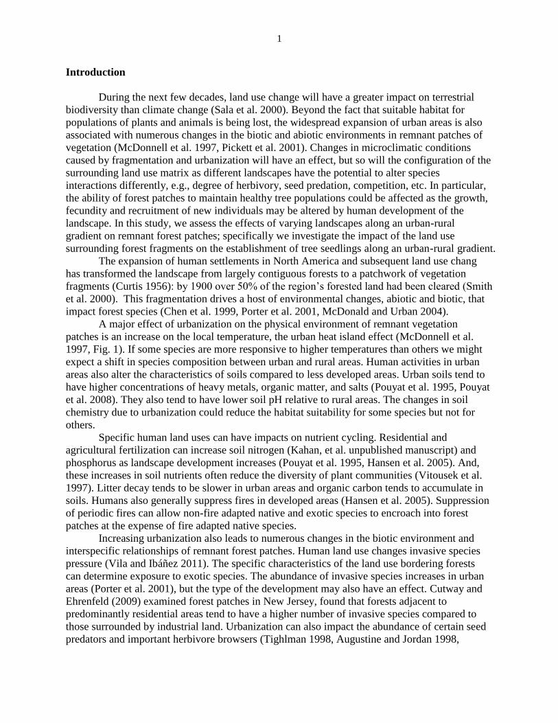
A major effect of urbanization on the physical environment of remnant vegetation

patches is an increase on the local temperature, the urban heat island effect (McDonnell et al.

1997, Fig. 1). If some species are more responsive to higher temperatures than others we might

expect a shift in species composition between urban and rural areas. Human activities in urban

areas also alter the characteristics of soils compared to less developed areas. Urban soils tend to

have higher concentrations of heavy metals, organic matter, and salts (Pouyat et al. 1995, Pouyat

et al. 2008). They also tend to have lower soil pH relative to rural areas. The changes in soil

chemistry due to urbanization could reduce the habitat suitability for some species but not for

others.

Specific human land uses can have impacts on nutrient cycling. Residential and

agricultural fertilization can increase soil nitrogen (Kahan, et al. unpublished manuscript) and

phosphorus as landscape development increases (Pouyat et al. 1995, Hansen et al. 2005). And,

these increases in soil nutrients often reduce the diversity of plant communities (Vitousek et al.

1997). Litter decay tends to be slower in urban areas and organic carbon tends to accumulate in

soils. Humans also generally suppress fires in developed areas (Hansen et al. 2005). Suppression

of periodic fires can allow non-fire adapted native and exotic species to encroach into forest

patches at the expense of fire adapted native species.

Increasing urbanization also leads to numerous changes in the biotic environment and

interspecific relationships of remnant forest patches. Human land use changes invasive species

pressure (Vila and Ibáñez 2011). The specific characteristics of the land use bordering forests

can determine exposure to exotic species. The abundance of invasive species increases in urban

areas (Porter et al. 2001), but the type of the development may also have an effect. Cutway and

Ehrenfeld (2009) examined forest patches in New Jersey, found that forests adjacent to

predominantly residential areas tend to have a higher number of invasive species compared to

those surrounded by industrial land. Urbanization can also impact the abundance of certain seed

predators and important herbivore browsers (Tighlman 1998, Augustine and Jordan 1998,

2

Rizkalla and Swihart 2009). Many vertebrates that are part of forest communities have particular

patterns of population density along urbanization gradients. Herbivores can have a substantial

impact on forest regeneration (Tilghman 1989, Augustine and Jordan 1998). Many species of

herbivores have population density patterns associated with human land use types. For example,

white-tailed deer (Odocoileus virginianus) have higher population densities in forest patches at

intermediate distances from urban centers than where forest patches are found within a matrix of

agriculture and low density development (Tilghman 1989). High levels of deer browsing can

impede the ability of slow growing species to regenerate.

Land-use change can also affect the soil microbial communities by altering nutrient

inputs (Peacock et al. 2001). Many urban soils have lower soil microfauna and fungal densities

and higher bacterial densities. Groffman et al. (1995) found lower microbial biomass in urban

versus rural soils. Other studies have shown higher rates of litter decomposition in urban versus

rural forests (Pouyat et al. 1996). Goldman et al. (1995) found higher potential N mineralization

rates in rural forests and higher nitrification rates in urban forests along a 140 km transect

stretching northward from New York City. Also earthworms tend to increase in abundance in

urban areas (McDonnell et al. 1997), and their presence and abundance can have profound

impacts on soil nitrogen chemistry (Steinberg et al. 1997). These soil community differences

combined with litter quality differences and increased temperatures in urban areas may explain

altered biogeochemical cycling in urban soils.

Through their interactions with forest species, these changes in biotic communities can

have substantial impacts on community composition in remnant vegetation patches. In the case

of tree species, tree mortality is heavily weighted towards early life stages (Harcombe 1987). In

particular, the biggest population bottlenecks for tree species are the seed and seedling stages.

Seedlings are a particularly vulnerable life history stage for trees. As such, seedlings could be

very sensitive to the abiotic and biotic gradients associated with the landscape matrix

surrounding forest fragments. Therefore, comparing seedling growth and mortality among tree

species at different sites along an urbanization gradient can provide an excellent indicator of how

land use impacts forest regeneration. This information will be paramount in understanding how

the combination of land use change and climate change will impact forest in coming decades.

Here we seek to address how human land use impacts population dynamics, i.e.,

recruitment of new individuals, within forest fragments along an urbanization gradient.

Specifically we test how the composition of the land use matrix impacts growth and mortality of

different tree seedlings and how this effect compares to other environmental factors. The specific

questions we aim to address in our work are: 1) Does land use surrounding a site have the

potential to impact regeneration of forest tree species? 2) What is the importance of the

surrounding landscape with respect to other environmental variables in tree seedling recruitment?

3) Do species differ in their responses to the land use matrix surrounding forest fragments?

Answers to these questions will allow a greater understanding of how the configuration of a

landscape impacts tree species regeneration within remnant vegetation patches. Information

derived from this work will also be critical in our efforts to predict future forests ability to adapt

to global change in the context of a shifting landscape.

3

Methods

We carried out a tree seedling transplant experimental along a 40 km transect stretching

from Ann Arbor, MI (urban center) to rural Livingston County (42°16′53″N 83°44′54″W; Fig. 1).

This experimental set up was designed to ensure that the land-use matrix surrounding our study

sites encompassed a variety of levels of urbanization and human use. For two summers, we

transplanted seedlings of dominant tree species into edge, middle and interior plots to capture the

effects of a variety of habitat types within each landscape. During the growing season, we

recorded individual seedling survival and measured growth in height at the end of the summer.

With these data, we modeled species-specific survival and growth based on individual seedling

responses to the landscape surrounding each site, their habitats, and other environmental factors.

This type of inference allowed us to make predictions, probability of survival and maximum

growth rate, about each species performance under a gradient of environmental conditions and

land-uses.

Study sites

We obtained 2005 land use data for the study area from the Southeast Michigan Chamber

of Governments1. We created a simplified land use classification system with six categories,

developed, agricultural, open, forest, water and wetland, using ArcMAP 10 (ESRI 2010). To find

the extent of each land use surrounding our study sites, we calculated a 1 km circular buffer

around each sites centroid. We then estimated the area of each land use type surrounding each

site.

Our four study sites were located along a 40 km urbanization gradient running from the

city of Ann Arbor northwest to rural Livingston County (Fig. 1). The most urban site (UR) was

located in Miller Woods, an Ann Arbor City Park. This 9.1 ha park is situated in a residential

neighborhood, and within 1 km 97.8% of the land is developed and 2.2% forested. The forest is

dominated by Acer negundo, Juglans nigra, Ailanthus altissima, Lonicera maackii and Populus

deltoids.

The first suburban site (SU1) was located in Radrick Forest, a 18 ha mixed-oak research

forest located on University of Michigan property approximately 8 km east-northeast of Ann

Arbor, MI. Within 1 km of SU1, 57.9% of the land is developed and 13.2% is forested (Fig. 1).

The second suburban site (SU2) was located in a mixed-oak forest in Stinchfield Woods,

a 314 ha University of Michigan research forest approximately 30 km northwest of Ann Arbor.

The land within 1 km of SU2 is 12.9% developed and 78.8% forested (Fig. 1).

The rural site (RU) was located in an oak-hickory forest in the Edwin S. George Reserve,

a 525 ha fenced research preserve that belongs to the University of Michigan. Within 1 km of

RU 0% of the land is developed and 54.7% is forested (Fig. 1).

Within each site, plot locations were selected to account for the natural variability of

microhabitats and edge effects. Studies of edge effects in temperate forests measure

environmental factors along transects of varying distances: Matalack (1993) used 40 m transects;

Chen et al. (1999) measured environmental change across 60 m transects; Moffatt et al. (2007)

used transects up to 250 m in length; Hewitt and Kellman (2004) defined forest interior as

greater than 50 m from forest edge in their transect experiment. Several studies that measure

environmental change relative to edges (e.g., Chen et al. 1995, Chen et al., 1999) show relative

stability in many environmental factors beyond 50 m – 60 m from the edge. In order to capture

1 www.semcog.org

4

the variation in microenvironmental factors due to edge effects, we planted seedlings into three

types of plots at each site: edge, middle and interior. Pairs of edge plots were located at forest

edges. Pairs of middle plots were located 30 m into form forest edges. Pairs of interior plots were

located 60 m from forest edges.

Planting and censuses

In order to capture the community level impact of surrounding land use on forests

regeneration, we selected a variety of representative forest species from several functional

groups, i.e., pioneer, mid-successional and late successional species, in addition to two invasive

species (Celastrus orbiculatus and Elaeagnus umbellata) (Table 1). Seeds collected from nearby

wild populations were germinated in a greenhouse and transplanted into field sites after the last

spring frost: early June in 2010, mid-May in 2011. We planted 15 individuals from each species

into rows 25 cm apart. The seedlings were separated by 25 cm in each row. Before planting

seedling height was recorded. After planting, seedling survival was monitored every 3-4 weeks

during the growing season. At the end of the growing season, seedling height was recorded at

field sites.

Soil moisture and light data

Volumetric soil water content was measured in the top 7.5 cm of soil during each census

with a FieldScout TDR 300 Soil Moisture Meter (Spectrum Technologies, Plainfield, IL, USA).

Four soil moisture measurements (one at each corner) were taken for each seedling plot at each

census. For our analysis, average summer soil moisture values for each plot were used. We

estimated the proportion of full sunlight each seedling received from hemispherical canopy

photographs (Rich et al. 1993). In August a photograph was taken above each seedling plot.

Photographs were taken with single lens reflex camera with a Sigma 8 mm 1801 fish-eye lens a

(Ronkonkoma, NY, USA). From these photographs, the proportion of full sunlight reaching the

forest floor at each plot, the global site factor (GSF), was calculated using the software package

HEMIVIEW (Delta-T Devices, Cambridge, UK).

Model of seedling survival

To be able to account for both the abiotic factors affecting seedling survival and the

impacts derived from the effects of the surrounding landscape we used a counting process in a

Cox survival model (Andersen et al. 1993). This type of survival model allows the inclusion of

fixed and random effects in the frailty or risk portion (Clark 2007). Here the data for each

seedling we studied and each time t, Nit, is coded as 0 if the seedling is alive or as 1 if the

seedling was recorded as dead that period of time, which would be the last time period accounted

for. The likelihood of the model accounts for the number of failures at each time:

( )

where the mean λ is then estimated as a function of the intrinsic rate of mortality, or hazard h,

and the extrinsic risk of mortality, or risk μ.

5

Parameters in the model were then estimated following a Bayesian approach that allowed

us to consider the different sources of uncertainty associated with the data, the process, and the

parameters (e.g., Clark 2007, Gelman and Hill 2007). The hazard was estimated at the species

level for each time step, ht, from a gamma distribution with non-informative parameter values,

ht~Gamma (0.01, 0.01). This intrinsic mortality rate would then reflect the temporal variability in

mortality that is not accounted for by the risk function.

The risk, μi, was estimated as a function of the covariates includes in the analysis, μi =

XiΒ. Xi is the matrix of covariates associated to each seedling i. Β is the vector of fixed effect

coefficients associated to each covariate. We tried several combinations of covariates and

random effects (e.g., plot and year) and selected the model that best predicted the data. For the

final survival model the covariates included in the analysis were: seedling height at the time of

planting, soil moisture, light level, and habitat type (edge, middle, or interior), this last variable

combined with landscape type (urban, suburban 1, suburban 2 and rural). Height, soil moisture,

and light measurements were standardize to facilitate convergence of the model runs.

( ) ( ) ( )

To account for the varying impact of habitat type depending on the surrounding

landscape, habitat was nested within landscape in a hierarchical framework (Fig. XX),

αlandscape,habitat~Normal(αlandscape, σ2landscape) where αlandscape~Normal(0,10000) and

σlandscape~Uniform(0,1000). Parameters were estimated from normal distributions with non-

informative parameter values, k~Normal(0,10000). To test the difference between the landscape

and habitat combinations (parameters landscape,habitat), we estimated the difference between the

associated parameters; a significant difference would then have a 95% credible interval around

the posterior mean that does not include zero. We report parameters α and multiply by -1 to

reflect their effect on survival (the Cox model estimates mortality).

Models were run in OpenBUGS 1.4 (Thomas et al. 2006); simulations were run until

convergence of the parameters was ensured (~25,000 iterations). Models were then run for

another 100,000 iterations from which posterior parameter values and predicted survival rates

were estimated. Final model selection was based on DIC (Deviance Information criterion), the

model with the lowest values of DIC was selected (Spiegelhalter et al. 2000). Predicted survival

for each species in each site habitat combination, ̂ , was estimated for average

height seedlings under habitat-specific average soil moisture and light conditions for the summer.

Model of seedling growth

As with seedling survival, we modeled seedling growth at the individual level. Only

seedlings that exhibited positive growth over the study period were included in the analysis (as

negative growth might have indicated herbivory or a substantial measuring error). Also, when

fewer than five individuals of a species at a given site-habitat combination survived the summer

those individuals were removed from the analysis, as the data would not have been sufficient to

estimate growth under those conditions. Total growth, the difference between height at planting

and final census, was modeled as a saturation function of light (Pacala et al., 1994, 1999 et al.

2003, Kobe 2006, Mohan et al. 2007). The growth of individual i was modeled as follows:

( )

6

Where is the species specific variance, ( ), and comes from the

light saturation equation:

here is the maximum growth for an individual modeled as function of landscape and

habitat (ln transformations were used to ensure positive growth values):

( ) ( )

The mean of the log normal distribution is estimated for each landscape and habitat combination

such that , and

( ). The amount of light

needed for growth to begin, , was estimated as . Here we estimated

k as 1~logNormal(0,10000) and 2~Normal(0,10000)..

The half saturation point, was

calculated as , 1~logNormal(0,10000) and 2~Normal(0,10000).

To ensure and were positive, their values were constrained between 0 and 1.

The model was run with two chains of parameters until convergence (~50,000 iterations)

The model was then run for an additional 100,000 iterations from which posterior parameter

values were estimated. To test the difference between the different landscape and habitat

combinations, we estimated the difference between the associated parameters

( ); a significant difference would then have a 95% credible interval around the

posterior mean that does not include zero. Significance was determined for the other covariates

(2, and 2) if the 95% credible interval did not contain zero.

Integrated assessment of seedlings performance

For those landscape-habitat combinations we have sufficient data, we calculated an

integrated assessment of species performance by multiplying predicted survival

( ̂ ) and maximum growth rate parameters ( ).

7

Results

Survival Model

Hazard

Hazard, a species intrinsic probability of mortality at each census, varied over the course

of the growing season (Supplemental Information). Hazard curves were diverse among species.

Several species, Acer saccharum, Elaeagnus umbellata, Prunus serotina, Quercus rubra, and Q.

velutina, experienced increasing mortality probability until the second or third census, after

which mortality decreased, this is a common trend in transplant experiments reflecting a delayed

transplant shock. Three species, Celastrus orbiculatus, Nyssa sylvatica, and Robinia

pseudoacacia, had hazard curves that increased throughout the growing season.

Landscape effects

The impact of landscape type on survival (αlandscape comparisons) was only different

among landscape types for E. umbelata, where urban and rural plots had higher survival than the

suburban sites (Table 2). For the other species significant differences took place between

particular landscape type and habitat combinations (Fig. 2). For A. rubrum survival in rural

middle and interior, but not edge, plots was higher than in urban and suburban sites. For A.

saccharum we observed the same pattern except that urban middle plots had survival rates as

high as those in the rural plots. Quercus rubra had higher survival in some urban sites in

comparison with suburban sites. Robinia pseudoacacia was the only species with higher survival

in suburban sites than in urban and rural ones.

Habitat effects

While looking at each landscape site we were able to assess the effect of habitat on

seedling survival (αlandscape, habitat comparisons). Results again varied among the studied species

and landscape sites, with no overall patterns of particular habitats always benefiting or reducing

survival (Table 2). A. rubrum survival was higher in interior and middle habitats than at the

forest edge in all landscape types. A. saccharum had significantly higher survival in middle than

in edge plots in the urban landscape. In one of the suburban settings C. orbiculatus showed

higher survival in the interior plot than at the edge of the forest. And N. sylvatica’s survival only

significantly varied in the rural plots, with higher survival in the middle and interior with respect

to the edge.

Effects of the covariates (soil moisture, light, planted height) on survival

The effect of soil moisture on seedling survival was significant, and positive, for A.

saccharum, C. orbiculatus, and N. sylvatica (Table 2). High light levels had also a positive effect

on A. saccharum and E. umbellata (Table 2). The variability on initial seedling height at the time

of planting it does not seem to have influenced survival during the summer (Table 2). And

although no significant, there is a trend for most species to have higher survival under high soil

moisture and light levels.

Growth Model

Landscape effects and light requirements

8

We used the values of the parameters landscape,habitat, lo (1) and (1) to compare species

according to their light requirements and growth responses (Table 3). The effects of landscape

habitat combination on seedling growth (landscape,habitat) do not show strong patterns for any of

the studied species (Table 3). For several species, A. saccharum, C. glabra, E. umbellata, N.

sylvatica, and Q. velutina, most combinations seem to have similar maximum growth rates. At

the urban site R. pseudoacacia experienced a higher growth rates, but only on at the edge and

middle sites (Fig. 3). And suburban habitats were best for C. orbiculatus and P. serotina. Across

sites, A. saccharum had the lowest maximum growth rate in edge sites. The light levels required

to start growth for average height seedlings varied among the species, with P. serotina and Q.

velutina having the highest and the two invasive species, C. orbiculatus and E. umbellate, the

lowest. The half saturation constant (parameter at average soil moisture) ranked P. serotina

and R. pseudoacacia at the top and A. saccharum and E. umbellata at the bottom (Table 3).

Effects of the covariates (soil moisture and planted height) on growth

All species had a significant response to soil moisture, the higher the level or soil

moisture the less light needed to reach the half maximum growth rate. However, the effect of soil

moisture varied among species (Table 3). Generally, the more shade tolerant species, N. sylvatica

and A. saccharum needed less soil moisture to reach their half maximum growth rate, while more

light demanding species, C. orbiculatus, E. umbellata, Q. velutina and R. pseudoacacia needed

more soil moisture to reach maximum growth under high light conditions. With respect to

planted height, only A. sccharum and C. orbiculatus showed a significant response. For these

three species, larger seedlings needed less light to begin growing. C. orbiculatus showed the

strongest response to planted height.

Integrated assessment of seedling recruitment.

Integrated performance, the product of predicted survival and maximum growth, showed

how each species preformed at each landscape-habitat combination (Fig. 4). At the urban site, E.

umbellata performed well at all site habitat combinations, though A. saccharum surpassed it in

the middle plots. At the suburban1 site, R. pseudoacacia preformed the best at the edge plots, E.

umbellata performed the best at the middle plots and C. orbiculatus preformed the best at the

interior plots. At the suburban2 site, C. orbiculatus and P. serotina preformed the best at the

edge plots while E. umbellata preformed the best at the middle and interior plots. At the rural site,

A. saccharum and C. orbiculatus preformed the best, while A. saccharum preformed the best at

the middle and interior plots.

9

Discussion

In this study our goal was to quantify the ability of dominant tree species to recruit new

individuals in remnant forest patches along an urban-rural gradient. Besides changes in the

microclimate conditions of these forest patches, forest fragments have the potential to also be

affected by the surrounding landscape. Distinct types of landscapes, e.g., agricultural land vs

urban development, may exert a different influence in forest patches by shaping some species

interactions that are critical for recruitment, e.g., seed predation, herbivory, plant-soil feedbacks.

Though there is substantial literature on the impacts of individual abiotic gradients on tree

seedlings, few studies have explored the impacts of the unique environments created by the

combinations of biotic and abiotic factors found along urbanization gradients.

By comparing survival and growth rates among species growing within different land use

matrices our results show that species vary in their responses to the unique environments

imposed by the combination of landscape and habitat. In addition, results also indicate that these

trends in seedling survival and growth also differed among species. This has potential

implications for forest regeneration as some species may have higher recruitment rates than

others at different landscapes.

Effects of the surrounding landscape on tree seedling survival

In our results, the overall effect of landscape type on seedling survival had a significant

impact on only one species, E. umbellata (Table 2). The invasive E. umbellata had higher

survival in the urban and rural sites than the suburban sites. It is possible E. umbellata

experienced greater mortality at the suburban sites due to factors not taken into account in our

study including herbivory and/or fungal pathogens. But this general lack of significance among

landscape types reflected the large variability of performances observed at each of those

landscape types (Table 2). Results indicate species-specific responses to each landscape-habitat

combination. Such range of variation suggests that the overall impact of landscape type is

complex and it interacts with the differential effects of the habitats nested within each landscape.

Once soil moisture and light were accounted for, results still point out at differences in

survival among habitats and sites (Table 2), and suggest there are factors beyond just the

environmental variables included in the analysis that are impacting the survival of the species at

these site-habitat combinations. Although soil moisture values did not correlate with habitat,

there was a strong relationship between habitat type and light: edge plots had the highest light

levels within each site while middle and interior plots had lower light levels (Fig. 5). The

survival model showed light had a significant effect on the survival of two species, A. saccharum

and E. umbellata. Interestingly, E. umbellata tended to have a stronger site-habitat effect (Fig. 9)

in sites with lower light levels. Similarly, the impacts of site-habitat on A. saccharum survival

were the most positive in the lower light interior plots (Fig. 9) indicating that the regeneration

niche is defined by more variables than those we measured.

The unique environments created by the combination of landscape and habitat could

explain the differences between site-habitat survival rates for some species. The importance of

the different habitats to seedlings survival depended on site for some species. For example, the

effects of site-habitat on Nyssa sylvatica do not differ greatly for all the sites except at the rural

site. There, N. sylvatica had significantly higher survival in the middle and interior plots than at

the edge (Fig. 11). Additionally, A. rubrum had the highest parameter values at the rural site, but

10

only at the middle and interior habitats (Fig. 9). Indeed, the predicted survival results (Fig. xx)

show for most species and at most site-habitat combinations, interior plots tended to have higher

survival.. This relationship was true even for A. saccharum and E. umbellata, the two species

whose survival was positively impacted by light despite light levels being lower in the interior

plots (Fig. 9).

Effects of landscape type and habitat on seedling growth

The results of the growth model add greater depth to the predictions of forest

regeneration across the landscape. Despite limited results, some species tended to have a higher

maximum growth rate in specific landscapes (Fig. 3). A. saccharum showed a higher maximum

growth in the urban and rural site, while C. orbiculatus had the highest maximum growth rate in

the rural site and in one of the suburban sites. R. pseudoacacia had its highest growth rate at the

urban site.

Generally there were few significant differences in maximum growth between the various

site-habitat combinations. This could be due to the fact that we measured growth in first year

seedlings that are still highly dependent on the seed resources. This would also explain the very

low values estimated for minimum amount of light required to start growth and the level of light

needed to reach half of the maximum growth rate. Still we were able to observe some patterns.

The habitat type within different landscapes altered maximum growth rates for some

species. A. saccharum and E. umbellata tended to have the highest maximum growth rates in

interior plots at all landscapes even if these two species highly depended on light to survive.

Other species had their highest maximum growth rate at a particular site-habitat combination.

For example, R. pseudoacacia had significantly higher maximum growth in the edge and middle

habitats at the urban site (Figure 3). Thus we might expect it to have a competitive advantage in

this location relative to the other site-habitat combinations.

Implications for future forests (integrated assessment)

Human land uses alter the environment in forest patches by decreasing interior habitat,

increasing temperature, changing nutrient cycling and patterns of animal abundance. Other than

affecting the local environment (e.g., light, soil moisture), very little attention has been given to

the potential effect of the surrounding landscape on these forest patches (but see McDonnell et al.

1997, Pickett et al. 2001). And in particular, there is practically no work looking at how the

combination of landscape structure and microsite, i.e., habitat, may play a role on tree species

recruitment of new individuals. For example, recruitment sites at the edge of a forest may be

highly favorable for light demanding species as light levels are usually higher (Whitmore &

Brown 1996, Coates 2001), but the degree at which this is a favorable site may also be

influenced by the herbivory pressure associated with that particular location. As deer densities

tend to be higher in suburban landscapes than in more rural areas or urban centers, seedlings

recruitment in edge sites may be jeopardize in suburban forest patches but highly favored in rural

and urban areas.

Our results show forest species respond differently to the environments created by

anthropogenic land uses. Some species in the study had higher survival at particular locations

along the urbanization gradient: Robinia pseudoacacia had higher survival in the two suburban

sites; Celastrus orbiculatus and E. umbellata had the highest survival at the urban site; A.

11

rubrum had higher survival in the middle and interior plots of the rural site. These findings

suggest that in a scenario where the landscape experiences an expansion of urban areas, species

such as A. rubrum may lose out to species with higher survival in the more suburban and urban

forests. Conversely, with regeneration of forests from agriculture abandonment, species favored

by more rural landscapes may increase in abundance. Other species, e.g., Q. rubra, whose

survival is not significantly impacted by landscape may not experience changes in abundance

with increased urbanization (Fig. 2).

These differences in recruitment will shape future forests’ structure and function, and

consequentially affect the forests’ potential to response to other drivers or change, e.g., global

warming, pollution, and/or invasive species. Therefore, forests capacity for carbon sequestration,

replenishment of the water table, and soil retention may also be altered not only by the extent and

location of future forests but also by the specific composition of their surrounding landscapes.

The results of our integrated performance metric suggest which of our study species may

be “winners” at specific points along our urbanization gradient (Fig. 4). The results from the

integrated performance show that in the more urban landscapes the invasives, C. orbiculatus and

E. umbellata out preform the majority of native species. However, at the rural site many of the

native species had performance that was on par with the invasives.

There are many other environmental variables that affect seedling growth and survival

that our study does not take into account: soil type, nutrients, heavy metal pollution, herbivory

(large and small mammal, insects), mycorrhizal associations, incidence of soil pathogens, etc.

Still we were able to observed and quantified recruitment patterns along a landscape gradient.

Our results indicate the need for further studies that focus on the actual mechanisms giving raise

to those patterns.

Conclusions

Most forests in eastern North America are being influenced by the human uses of the

landscape surrounding them (Riitters et al. 2012). Pristine forests are rapidly disappearing and

more and more the only remnant patches of forested vegetation are those embedded in a matrix

of highly altered landscapes. However, most of our knowledge about tree species recruitment

dynamics comes mainly from studies in intact forests (Canham et al. 1990, LePage et al. 2000,

Siemann & Rogers 2003) and from old-field succession dynamics (De Steven 1991ab, Bakker et

al. 2004). And, even in this last setting, old-field succession, recruitment studies have mainly

focused on the particular conditions taken place at the microsite level, and a landscape

perspective is commonly missing.

Human alterations of the landscape affect forest species differently. Expansion of urban

areas, abandonment of agricultural land, and restoration of forested land can all have impacts on

the environment of adjacent forest patches and the species living in them. The effects of different

land uses on the survival and growth of tree species could have a tremendous impact on how

forests respond to future stresses such as climate change and species invasions. The ability of

forests to provision essential ecosystem services (i.e., water, pollution control, soil retention) and

their stability and resilience to disturbances depends on the species composition of these forests

(Tillman 1996). Therefore understanding the complex effects of human land use on forests is

essential to ensure forests continue to provide these services humans depend upon.

12

Literature Cited

Augustine, D. J. and P. A. Jordan. Predictors of White-Tailed Deer Grazing Intensity in

Fragmented Deciduous Forests The Journal of Wildlife Management, Vol. 62, No. 3 (Jul., 1998),

pp. 1076-1085

Curtis, J. T. 1956. The modification of mid-latitude grasslands and forests by man. In Man’s

Role in Changing the Face of the Earth, W. L. Thomas ed. Chicago: University of Chicago Press.

Chen, J., S. C. Saunders, T. R. Crow, R. J. Naiman, K. D. Brosofske, G. D. Mroz, B. L.

Brookshire, and J. F. Franklin. 1999. Microclimate in forest ecosystem and landscape ecology.

BioScience 49: 288-297

Clark, J. S., B. Beckage, P. Camill, B. Cleveland, J. HilleRisLambers, J. Lichter, J. McLachlan, J.

Mohan, P. Wykoff. 1999. Interpreting recruitment limitation in forests. American Journal of

Botany, 86: 1-16.

Clark, J. S. 2007. Models for Ecological Data: An Introduction. Princeton University Press.

Cutway, H. B., and J. G. Ehrenfeld. 2009. Exotic plant invasions in forested wetlands: effects of

adjacent urban land use type. Urban Ecosystems 12: 371-390

Goldman, M.B., Groffman, P.M., Pouyat, R.V., McDonnell, M.J., Pickett, S.T.A., 1995. CH4

uptake and N availability in forest soils along an urban to rural gradient. Soil Biology and

Biochemistry 27, 281–286.

Groffman, P.M., Pouyat, R.V., McDonnell, M.J., Pickett, S.T.A., Zipperer, W.C., 1995. Carbon

pools and trace gas fluxes in urban forest soils. In: Lal, R., Kimble, J., Levine, E., Stewart, B.A.

(Eds.), Soil Management and Greenhouse Effect. CRC Press, Boca Raton, Florida, pp. 147–157.

Hansen, A. J., R. L. Knight, H. M. Marzluff, S. Powell, K. Brown, P. H. Gude, and K. Jones.

2005. Effects of exurban development on biodiversity: patterns, mechanisms, and research

needs. Ecological Applications 15: 1893-1950.

Hewitt, N., and M. Kellman. 2004. Factors influencing tree colonization in fragmented forests:

an experimental study of introduced seeds and seedlings. Forest Ecology and Management 191:

39-59

Kahan, A. Y., W. S. Currie, and D. G. Brown. unpublished manuscript. Nitrogen and Carbon

Biogeochemistry in Soil and Vegetation Along a Urban-Rural Gradient in Southeastern

Michigan.

McDonnell, M. J., S. T. A. Pickett, P. Groffman, P. Bohlen, R. V. Pouyat, W. C. Zipperer, R. W.

Permelee, M. M. Carreiro, and K. Medley. 1997. Ecosystem processes along an urban-to-rural

gradient. Urban Ecosystems 1: 21-36.

13

McDonald, R. I., and D. L. Urban. 2004. Forest edges and tree growth rates in the North

Carolina Piedmont. Ecology 85: 2258-2265.

Moffatt, S. F., S. M. NcLachlan, and N. C. Kenkel. 2004. Impacts of land use on riparian forest

along an urban – rural gradient in southern Manitoba. Plant Ecology 174: 1573-5052

Pickett, S. T. A, M. L. Cadenasso, J. M. Grove, C. H. Nilon, R. V. Pouyat, W. C. Zipperer, R.

Costanza. 2001. Urban Ecological Systems: Linking Terrestrial Ecological, Physical, and

Socieoeconomic Components of Metropolitan Areas. Annual Review of Ecological and

Systematics 32: 127-157.

Porter, E. E., B. R. Forschner. 2001. Woody vegetation and canopy fragmentation along a forest-

to-urban gradient. Urban Ecosystems, 5: 131-151.

Pouyat, R. V., M. M. Carreiro, M. J. McDonnell, S. T. A. Pickett, P. M. Groffman, R. W.

Parmelee, K. E. Medley, W. C. Zipperer. 1995. Carbon and nitrogen dynamics in oak stand

along an urban-rural gradient. Pages 569-587 in J. M. Kelly and W. W. Mcfee, editors. Carbon

forms and functions in forest soils. Soil Science Society of America Monograph, Madison,

Wisconsin, USA.

Pouyat, R. V., I. D. Yesilonis, K. Szlavecz, C. Csuzdi, E. Hornung, Z. Korsos, J. Russell-Anelli,

and V. Giorgio. 2008. Response of forest soil properties to urbanization gradients in three

metropolitan areas. Landscape Ecology 23:1187-1203

Riitters, K., J. Wickham, R. O'Neill, B. Jones, and E. Smith. 2000. Global-scale patterns of forest

fragmentation. Conservation Ecology 4(2): 3. [online] URL:

http://www.consecol.org/vol4/iss2/art3/

Rizkalla, C. E. and R. K. Swihart. 2009. Forecasting the Effects of Land-Use Change on Forest

Rodents in Indiana. Environmental Management 44: 899-908

Sala, O., F. S. I. Chapin, J. J. Armesto, E. Berlow, J. Bloomfield, R. Dirzo, E. Huber-Sanwald, L.

F. Huenneke, R. B. Jackson, A. Kinzig, R. Leemans, D. M. Lodge, H. A. Mooney, M. Oesterheld,

N. L. Poff, M. T. Sykes, B. H. Walker, M. Walker, and D. H. Wall. 2000. Global biodiversity

scenarios of the year 2100. Science 287:1770-1774

Smith, W.B., Vissage, J.S., Darr, D.R., and Sheffield, R.M., 2000, Forest Resources of the

United States, 1997: St. Paul, MN, U.S. Department of Agriculture Forest Service.

Steinberg, D. A., RV Pouyat, RW Parmelee and P. M. Groffman. 1997. Earthworm abundance

and nitrogen mineralization rates along an urban-rural land use gradient. Soil Biology and

Biochemistry, 29: 427-430.

Vila, M. and Ibáñez, I. 2011 Plant Invasions in the landscape. Landscape Ecology, 26: 461-472

14

Vitousek, Peter M., John D. Aber, Robert W. Howarth, Gene E. Likens, Pamela A. Matson,

David W. Schindler, William H. Schlesinger, and David G. Tilman. 1997. HUMAN

ALTERATION OF THE GLOBAL NITROGEN CYCLE: SOURCES AND CONSEQUENCES.

Ecological Applications 7:737–750.

15

Table 1. Species list, years planted, growth, and habitat requirements.

Species Common Name Code 2010 2011 Growth Light Soil

Acer rubrum Red maple acru x x Moderately fast Mid tolerant Moist

Acer saccharum Sugar maple acsa x Slow Very shade tolerant Moist well drained

Carya glabra Pignut hickory cagl x Slow Mid tolerant Dry tolerant

Celastrus orbiculatus Oriental bittersweet ceor x x Rapid Sun to partial shade Dry tolerant

Elaeagnus umbellata Autumn-olive elum x x Rapid Sun to partial shade Dry tolerant

Nyssa sylvatica Black tupelo nysy x x Slow Shade-tolerant Wet-mesic

Prunus serotina Black cherry prse x Fast Mid tolerant Not wet tolerant

Quercus rubra Northern red oak quru x x Moderately fast Sun to partial shade Mesic

Quercus velutina Black oak quve x x Moderately fast Shade-intolerant Dry tolerant

Robinia pseudoacacia Black locust rops x Fast Shade-intolerant Not wet tolerant

Barnes & Wagner 2004, www.na.fs.fed.us/spfo/pubs/silvics-manual

16

Table 2. Parameter estimates from the Survival analysis, means and standard deviations. Statistically significant differences among

the alpha parameters for each landscape type and habitat combination are shown in Fig. 6. Values in bold for the covariates (soil

moisture [Υ1], light [Υ2], and planted seedling height [Υ3]) indicate the 95% credible interval around the posterior mean did not include

zero. E: edge habitat, M: middle habitat, and I: interior habitat.

Urban Sub1 Sub2 Rural

E M I E M I E M I E M I Urban Sub1 Sub2 Rural SoilM Light Height

Parameter α site,habitat α site,habitat α site,habitat α site,habitat α site γ1 γ2 γ3

acru mean 2.11 3.17 3.84 1.97 2.81 2.98 0.47 3.53 3.07 1.58 5.57 5.77 3.00 2.55 2.31 4.24 -0.04 1.01 1.97

sd 0.74 0.76 0.86 0.65 0.68 0.68 2.68 0.71 0.71 1.77 1.05 1.22 7.52 6.17 10.80 12.52 0.17 0.66 2.14

acsa mean 1.18 5.74 1.98 2.41 2.19 2.75 3.91 3.01 3.87 5.42 7.18 15.12 2.19 3.20 5.42 0.54 2.07 0.21

sd 0.82 1.39 ### 0.61 0.82 0.68 1.99 0.66 0.60 1.32 0.88 1.53 45.16 5.35 8.78 11.03 0.27 0.77 1.47

ceor mean 5.81 5.36 5.24 2.78 4.19 5.43 4.85 5.20 4.56 4.40 6.21 ### 5.44 4.12 4.85 14.49 1.35 0.93 -1.16

sd 1.28 0.99 1.04 1.10 1.35 1.43 2.20 0.95 0.87 1.71 1.47 ### 6.29 9.47 8.37 41.07 0.38 1.05 1.93

elum mean 6.69 8.09 2.92 3.96 4.53 5.45 4.95 7.94 7.60 13.06 3.80 1.35 4.00 -0.10 2.56 8.06

sd ### 1.52 1.77 1.04 1.10 1.10 5.89 1.11 1.15 4.19 1.62 1.96 34.03 7.92 20.39 19.70 0.29 1.07 4.54

nysy mean 2.59 2.43 2.17 2.15 2.22 2.44 2.42 2.80 2.72 1.70 3.52 3.88 2.39 2.27 2.63 3.01 0.34 0.46 0.48

sd 0.58 0.53 0.54 0.50 0.54 0.53 1.06 0.49 0.48 0.84 0.54 0.63 4.57 4.18 5.51 8.93 0.15 0.35 0.82

prse mean 4.02 3.25 3.52 10.73 2.44 3.00 7.31 2.38

-

0.24 3.59 5.20 3.04 0.20 -1.86 -6.35

sd 0.93 1.50 1.32 7.30 1.70 1.68 5.24 2.09 2.78 6.06 17.30 16.19 0.27 1.44 6.37

quru mean 2.93 3.12 2.96 2.59 2.72 2.57 2.72 2.69 2.44 2.18 3.00 2.83 3.01 2.61 2.62 2.68 0.06 -0.12 0.37

sd 0.57 0.56 0.57 0.56 0.62 0.58 0.93 0.50 0.49 0.84 0.53 0.56 3.58 3.26 5.31 5.84 0.13 0.39 0.76

quve mean 2.05 2.73 2.18 2.95 2.75 3.13 3.43 2.98 2.85 2.53 3.29 3.77 2.30 2.95 3.06 3.21 0.10 0.21 -0.03

sd 0.57 0.54 0.52 0.52 0.56 0.57 1.01 0.49 0.48 0.79 0.54 0.64 5.30 4.24 5.26 6.94 0.14 0.40 0.74

rops mean 2.46 2.27 2.44 4.18 3.91 3.69 3.97 3.88 3.48 2.76 2.87 2.98 2.37 3.90 3.76 2.87 0.10 -0.71 0.70

sd 0.75 0.59 0.63 0.67 0.70 0.67 0.92 0.58 0.56 0.74 0.56 0.61 4.12 4.43 5.46 4.05 0.22 0.53 0.64

17

Table 3. Parameter estimates from the growth model, posterior means and standard deviations. Statistically significant differences

among the parameters for each landscape type and habitat combination are shown in Fig. 9. Values in bold for the covariates (β2, and Υ2) indicate the 95% credible interval around the posterior mean did not include zero.

Urban Sub1 Sub2 Rural

E M I E M I E M I E M I

Parameter α α α α α α α α α α α α 1:lo 2:Height Υ1:θ Υ2:SoilM

acsa mean 3.27 5.69 4.82 3.58 5.04 5.26 - 3.91 4.01 3.91 5.55 5.65 0.0004 0.0182 0.8310 -0.9860

sd 0.40 0.27 0.27 0.38 0.27 0.21 - 0.45 0.39 0.25 0.23 0.17 0.0011 0.0068 0.0855 0.1138

cagl mean - - - - - - 3.03 4.45 3.73 3.50 4.40 4.68 0.0007 0.0171 0.5226 -0.7381

sd - - - - - - 0.27 0.65 0.69 0.37 0.70 0.82 0.0037 0.0147 0.2512 0.2243

ceor mean 3.22 3.32 - 3.71 - 4.85 3.93 - - 2.90 2.93 4.84 0.0000 0.0335 0.4594 -0.2006

sd 0.31 0.51 - 0.40 - 0.50 0.41 - - 0.46 0.52 0.44 0.0001 0.0108 0.0448 0.0017

elum mean 4.10 4.91 4.96 3.78 4.27 3.94 4.19 4.80 4.69 3.76 4.84 5.28 0.0002 0.0113 0.8475 -0.2849

sd 0.19 0.22 0.20 0.15 0.37 0.43 0.19 0.21 0.22 0.15 0.16 0.19 0.0005 0.0078 0.0670 0.0529

nysy mean - - - 3.13 - 5.05 2.63 - - 4.51 - 4.90 0.0010 0.0872 0.8140 -2.3960

sd - - - 0.38 - 0.61 0.58 - - 0.86 - 0.40 0.0017 0.1223 0.0843 0.0752

prse mean - - - - - - 2.96 1.95 - - 2.22 - 0.0094 -0.0248 0.0207 -0.4486

sd - - - - - - 0.46 0.30 - - 0.36 - 0.0172 0.0385 0.0277 0.2591

quve mean 2.57 3.64 - - - 3.89 3.35 - 3.22 - 4.74 4.40 0.0011 0.0133 0.2483 -0.1638

sd 0.63 0.52 - - - 0.44 0.31 - 0.30 - 0.40 0.29 0.0031 0.0145 0.0645 0.1028

rops mean 4.19 4.45 2.81 2.81 - 3.07 2.66 2.53 3.35 2.52 3.74 3.60 0.0003 -0.0063 0.0536 -0.1137

sd 0.21 0.27 0.30 0.24 - 0.35 0.40 0.37 0.31 0.42 0.40 0.25 0.0007 0.0157 0.0083 0.0090

18

Figure 1. Forest fragmentation and land use in Washtenaw and Livingston Counties, South East

Michigan. The extent of pre-settlement forest (A) has been greatly reduced to produce today’s

fragmented network of forest patches (B). Presently forests exist within a matrix of other land

uses (C) adding to the environmental from pre-settlement conditions. Study sites along of the

urban-rural gradient are indicated with a star (C).

19

Figure 2. Posterior means (+2sd) for the parameters αsite,habitat , indicating the effect that each landscape type and habitat combination

had in seedling survival. Letters indicate statistically significant differences among the different landscape habitat combinations.

Landscapes U: urban, SU1: suburban 1, SU2: suburban 2, R: rural. Habitats E: edge, M: middle, I: interior.

20

Figure 3. Impact of site-habitat combination on maximum growth rate (mm/summer). Posterior

means and +2sd). Landscape type U: urban, Sub1: suburban 1, Sub2: suburban 2, R: rural.

21

Figure 4. Integrated performance (mean+sd) for the studied species at each landscape type and

habitat combination. Integrated performance was estimated as the product of predicted survival

under average light and soil moisture conditions and predicted maximum annual growth.