The impact of FDI on Poverty Reduction in North Africa

HAL Id: hal-01756624https://hal.archives-ouvertes.fr/hal-01756624

Preprint submitted on 2 Apr 2018

HAL is a multi-disciplinary open accessarchive for the deposit and dissemination of sci-entific research documents, whether they are pub-lished or not. The documents may come fromteaching and research institutions in France orabroad, or from public or private research centers.

L’archive ouverte pluridisciplinaire HAL, estdestinée au dépôt et à la diffusion de documentsscientifiques de niveau recherche, publiés ou non,émanant des établissements d’enseignement et derecherche français ou étrangers, des laboratoirespublics ou privés.

The impact of FDI on Poverty Reduction in NorthAfrica

Marwa Lazreg, Ezzeddine Zouari

To cite this version:Marwa Lazreg, Ezzeddine Zouari. The impact of FDI on Poverty Reduction in North Africa. 2018.�hal-01756624�

https://hal.archives-ouvertes.fr/hal-01756624

https://hal.archives-ouvertes.fr

1

The impact of FDI on Poverty Reduction in North Africa

Marwa Lazreg *

Faculty of Economic Sciences and Management of Sousse

University of Sousse, Tunisia

E-mail: [email protected]

* Corresponding author

Ezzeddine Zouari

Faculty of Economic Sciences and Management of Sousse

University of Sousse, Tunisia

E-mail: [email protected]

Abstract: The aim of this paper is to study the impact of FDI on poverty in the case of the

North African country during the period from 1985 to 2005. The sample used in this paper

consists of 6 countries of North Africa during the period from 1985 to 2005. So we can use

the cointegration test. For the cointegration test, we have certified the existence of a

cointegration relationship between the different series studied in our paper. Indeed, the result

of the null hypothesis test of no cointegration was rejected at the 5% threshold, which

explains the presence of a cointegration relationship. Also, to test the effect of FDI on poverty

in the countries of North Africa, we will perform a FMOLS estimate. Thus, for the short-term

dynamics, we noticed that FDI have a positive and significant impact on a threshold of 1% on

the GINI index for the case of the countries of North Africa and a significant negative a

threshold of 1% for the other two indicators of poverty; LPOV1_91 $ and LPOV3_1 $. Then

we found that is statistically significant and positive at a 1% level. The LIDE variable

measuring foreign direct investment has a negative impact on the Gini index to a threshold of

5%.For the Granger causality test; we notice that there is a unidirectional relationship between

the consumption of energy and poverty Granger. Only the GINI index can cause Granger

consumption of energy.

Keywords: IDF; poverty; North Africa; cointegration; FMOLS

mailto:[email protected]

mailto:%[email protected]

2

1. Introduction

The indirect impact of FDI on poverty reduction through economic growth and FDI

relationship was widely covered in the literature. The majority of these studies assume that

what is good for growth is good for the poor (Sumner, 2005). The lack of a simple positive

impact of FDI on poverty reduction motivated investigations on the possible direct impact of

FDI on poverty reduction. The literature on the direct impact of FDI on poverty reduction is

still insufficient.

Although the Millennium Development Goal (MDG) of reducing extreme poverty and hunger

by 2015 has been met at the global level, some countries still experiencing high levels of

poverty. While the struggle for the eradication of poverty continues, the MDGs was signed in

2015 within the United Nations sustainable development goals, strengthening the pressure on

developed and developing governments to seek solutions to reducing poverty in national and

international relations.

The conflicting findings about the relationship between FDI and poverty reduction

policymakers have left a number of questions about the benefits that can be derived from

liberal policies that encourage FDI flows.

Existing studies, which are based on different countries, poverty indicators and various

econometric approaches, have failed to provide a conclusive answer to the link between FDI

and poverty.

The impact of FDI on poverty reduction has been the subject of much controversy and so far,

investigations are continuing in order to disentangle the possible benefits of FDI for poverty

reduction.

The literature on the impact of FDI on poverty is divided between the search for a positive

impact of FDI on poverty reduction, and a negative impact, or an insignificant impact of FDI

on reducing poverty.

Some of the positive contributions of FDI on poverty reduction are achieved through spillover

effects in job creation and increased investment capital (Meyer, 2004; Gorg and Greenaway,

2004). The literature that supports a negative or insignificant impact of FDI on poverty

reduction is covered by the dependency theory, which explains the underdevelopment of

developing countries and how the nature of development leads to poverty.

The spillover effects can be divided into two categories, namely horizontal and vertical. The

horizontal spillovers arising from non-contractual and non-market operations, where external

parties, in this case the domestic companies, benefit from resources from foreign companies

(Meyer, 2004).

These benefits are also called externalities (Meyer, 2004). According to Meyer (2004),

spillover effects in this category occur mainly in intra-industry configuration.

Thus, this paper has been devoted to relevant empirical study to clarify the impact of FDI on

poverty in the case of the North African country during the period from 1985 to 2005. The

sample used in our paper consists of 6 countries of North Africa during the period from 1985

to 2005. We concluded that on the basis of the test statistics of Im-Pesaran-Shin (IPS) test

ADF-Fisher and the test of PP-Fisher, we can conclude that only three variables LIDE, LPIB,

LINF and are stationary in LUE level. But first difference, all variables are stationary

according to these three tests. Thereafter, all the variables are integrated of order 1. Thus, we

can use the cointegration test. For the co-integration test, we have certified the existence of a

cointegration relationship between the different series studied in our paper. Indeed, the results

3

of the null hypothesis test of no cointegration were rejected at the 5% threshold, which

explains the presence of a cointegration relationship.

The results of these tests can determine the use of an error correction model. Also, to test the

effect of FDI on poverty in the countries of North Africa, we will perform a FMOLS estimate. Thus, for the short-term dynamics, we noticed that FDI have a positive and significant impact

on a threshold of 1% on the GINI index for the case of the countries of North Africa and a

significant negative a threshold of 1% for the other two indicators of poverty; LPOV1_91

LPOV3_1 $ and $. Then we found that is statistically significant and positive at a 1% level.

Noula LIDE variable measuring foreign direct investment has a negative impact on the Gini

index to a threshold of 5%. That is to say, if the level of FDI increased by 5 units, then the

GINI index decreases by 0.007476 units. For the Granger causality test, we noticed that there

is a unidirectional relationship between the consumption of energy and poverty Granger. Only

the GINI index can cause Granger consumption of energy.

The rest of the paper is organized as follows: In Section 2, we present a literature review. The

third section summarizes the econometric methodology. Data are presented in Section 4.

Section 5 was dedicated to the interpretation of results. The conclusion is made in section 6.

2. Literature review

Hung (1999) analyzes the relationship between FDI and poverty between 1992 and

2002 in a sample of 12 cities in Vietnam. He uses the incidence of poverty as a

measure of poverty. Hung (1999) finds that a 1% increase in FDI has reduced the

number of people living in poverty by 0.05%. This direct impact of FDI on poverty

reduction was rated higher than the indirect effects of GDP growth.

Similarly, Jalilian and Weiss (2002) study the relationship FDI-growth-poverty the

CountryASEAN (ASEAN). They took a sample of 26 countries including 18

ASEAN countries are developing and 8 developed countries, the authors use the

method of unbalanced panel data (unbalanced panel data) over a period from 1997

to 2007. Their econometric analysis shows that FDI inflows, particularly in the case

of ASEAN, are associated with higher economic growth and there is a close

relationship between the growth in average income and growth of income of the

poor. In their sample for ASEAN, on average, about 40% of the effects of FDI on

poverty reduction from economic growth and the remaining 60% are directly

related, so the results show a positive association between FDI and reduction

poverty

In the same way, Calvo and Hernandez (2006) examine the effects of FDI on

poverty in 20 American Country between 1984 and 1998. Based on panel data, the

authors used two dependent variables: the actual and the poverty gap. They found

that the benefits of FDI vary the initial local conditions and orientation of the foreign

subsidiary. They found that FDI reduce poverty on a global level. If foreign capital

has doubled, the number of poor declined. .

As for Nunnenkamp et al. (2007) use the CGE analysis to examine the effects ofFDI

Poverty in Bolivia. The authors used a model of a modified version of general

equilibrium which had 11 production sectors, 7 factors, and 6 types of households.

The simulation results showed that FDI improves economic growth and reduced

poverty. Other results showed that FDI generally widen income disparities between

urban and rural areas and, in particular, led to increased employment and

remuneration of the factors in urban areas.

4

Moreover, Reiter and Steensma (2010) conduct a study on the relationship between

human development captured by the human development index (HDI), and FDI in a

sample of 49 developing countries between 1980 and 2005. The sample consists of a

panel data set of 49 developing countries over the period 1980-2005, the authors use

the method of unbalanced panel data. The results were consistent with the results of

Jalilian and Weiss (2002). The relationship between FDI and improving human

development is also more strongly positive when corruption is low. So the results

show a positive association between FDI and poverty reduction.

Moreover, Zaman et al. (2012) have attempted to assess the impact of FDI on

poverty reduction in Pakistan. They took time series data over a period of 26 years

(1985-2011) based on a multi varied regression framework. . OLS estimates of the

results showed a coefficient of FDI, implying that the increase in FDI will result in

poverty reduction .They have concluded a positive link between FDI and poverty

reduction in Pakistan.

Mahmood and Chaudhary (2012) also study the contribution of FDI to the reduction

of poverty, lhe authors use the model of ARDL in Pakistan between 1973 and

2003.L'étude is the long-term relationship, short-term in the model. Government

spending on health and education as well as the rate of economic growth have

significant negative effects on poverty. The IDE helps therefore to reduce the level

of poverty in Pakistan.

Meanwhile, Shamim et al. (2014) empirically analyze the relationship between FDI

and poverty reduction in Pakistan. The period covered by this study was 1973-2011,

the model used is the technique of time series data cointegration (time series data

cointegration tehnique). The results showed that there was a positive relationship

between FDI and reduction poverty, as Fowowe and Shuaibu (2014) and Jalilian and

Weiss (2002).

Ucal (2014) also assess the relationship between foreign direct investment (FDI) and

poverty to the macro-way in some developing countries. In this study, the author

considers the unbalanced panel data method 26 countries in UNCTAD over a period

of 24 years between 1990 and 2009. The results show that there is a statistically

significant relationship between FDI and poverty. It is obvious that FDI reduces

poverty in some developing countries.

Besides, Bharadwaj (2014) studies the relationship between globalization and

poverty, the impact of real and financial integration on the counting rate and the

poverty gap. In the study, FDI was used as indicator of globalization, while the

population ratio and the poverty gap are indicated poverty Using a regression in 35

countries in the process of panel data development from 1990 to 2004, Baradwaj

(2014) shows that the growth and the opening of GDP per capita are beneficial for

the poor and FDI was considered beneficial for reducing poverty in countries in the

sample.

In parallel, Uttama (2015) studies the relationship between FDI and the reduction of

poverty. The data set includes transnational observations for six member countries

of ASEAN (Indonesia, Malaysia, Philippines, Singapore, Thailand and Vietnam)

during the period 1995-2011 using the technique of spatial panel data model, The

analyzes confirm the significant positive relationship between FDI and poverty

reduction in ASEAN, both individually and space.

3. Empirical Methodology

5

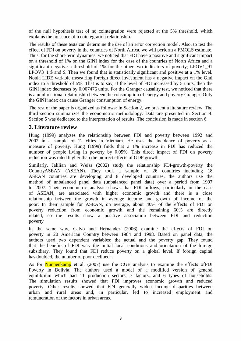
In our paper, we will use the model developed by Im and McLaren (2015) to study the impact

of FDI on poverty in the countries

of North Africa. The model used

was as follows:

Where POV poverty measure for each country, FDI measure foreign direct investment and V

represents a vector of control variables. Thus, the control variables, the growth rate of gross

domestic product (GDP), youth literacy rate (TAJ), financial development measured by

domestic credit to the private sector (DF), the urban population (PU ), government spending

(DEP) Market capitalization of listed companies (CBEC), the consumption or use of energy

(EU), the inflation rate (INF), energy use renouvlable (CER), the gross capital formation

(BCF) and the unemployment rate (CH).

Note that poverty is measured by three indicators:

The GINI index.

The poverty gap at $ 1.91.

The poverty gap of $ 3.1.

FDI is measured by the level of FDI to GDP for each country.

The models to estimate are:

0 1 2 3 4 5

6 7 8 9 10

11 12 13

2it it it it it it

it it it it it

it it it it

LGINI LIDE LCO LINF LPIB LPU

LTAJ LUE LDEP LDEF LFBC

LCH LCER LCBEC

(1)

0 1 2 3 4 5

6 7 8 9 10

11 12 13

1.91$ 2it it it it it it

it it it it it

it it it it

LPOV LIDE LCO LINF LPIB LPU


LCH LCER LCBEC

(2)

0 1 2 3 4 5

6 7 8 9 10

11 12 13

3.1$ 2it it it it it it

it it it it it

it it it it

LPOV LIDE LCO LINF LPIB LPU


LCH LCER LCBEC

(3)

Or, 0 is a constant, i are coefficients of the explanatory variables i = 1, ..., 13 and it it is the

term of error.

Table 1résume the different variables used in our paper.

Table 1: The different variables used Nature of factor The variable Code Variable Source

Dependent variable GINI Index GINI world Bank

Dependent variable Poverty to $ 1.90 a day (2011 PPP) (%) $ POV1.91 world Bank

Dependent variable Poverty to $ 3.10 a day (2011 PPP) (%) $ POV3.1 world Bank

Control variable CO2 emissions (kt) CO2 world Bank

Control variable Foreign direct investment, net inflows (% of

GDP) FDI world Bank

Control variable Youth literacy rate (% of youth aged 15 to 24) TAJ world Bank

,POV f IDE V

6

Control variable GDP per capita (annual%) GDP world Bank

Control variable Public expenditure (% of GDP) DEP world Bank

Control variable Use of renewable energy (% of total energy

consumed) CER world Bank

Control variable Inflation, consumer prices (annual%) INF world Bank

Control variable urban population (% of total) PU world Bank

Control variable Market capitalization of listed companies (%

of GDP) CBEC world Bank

Control variable Unemployment, total (% of population) (ILO

modeled estimate) CH world Bank

Control variable Gross capital formation (% of GDP) FBC world Bank

Control variable Domestic credit to private sector (% of GDP) DF world Bank

Control variable Energy use (kg oil equivalent) per $ 1,000

GDP (PPP constant 2011) EU world Bank

The data used in this paper are of annual frequency for all variables. These data come from

the World Bank database and the International Monetary Fund for the period from 1985 to

2015.We will estimate the models chosen by referring to an analysis of panel data.

The choice of panel data is based on the two dimensions of the data used; the first dimension

is time (a period of 31 years) and the second is individual (employee sample consists of 6

countries of North Africa).

4. Data

In this section, we present the sample and the model used in our paper. Our objective in this

paper, Is the study of the impact of FDI on poverty in the case of the North African country

during the study period between 1985 and 2015.

In Table 2, we exposed the different countries in our paper.

Table 2: The countries of North Africa Name of country Area (km) Population (2016 estimate) Population density (per km²)

Algeria 2381741 37,100,000 14.5

Egypt 1001450 81,249,302 80.4

Libya 1759540 6461450 3.7

Morocco 710 850 32,245,000 70.8

Sudan 1886068 31957965 16.9

Tunisia 163610 10673000 64.7

In this section we will try to make a descriptive analysis of the different results for the study

the impact of FDI on poverty in the countries of North Africa.

First, let's define the type of assessment which is a regression on panel data. Our choice is

justified by the presence of two dimensions in the data used; is the first time (a period of 31

years) and the second is individual (our sample is made up of 6 countries of North Africa).

This section is dedicated to the interpretation of results for the descriptive statistics and

Pearson correlation matrix for the variables used in our paper.

All of the descriptive statistics of the variables used in our paper are summarized in Table 3.

According to the results of Table 3, we found that the LCO2 variable, which expresses

logarithm of CO2 emissions, can reach a maximum value of 12.30497. As its minimum value

is 7.975197. Its risk is measured by the standard deviation is 1.022934.

7

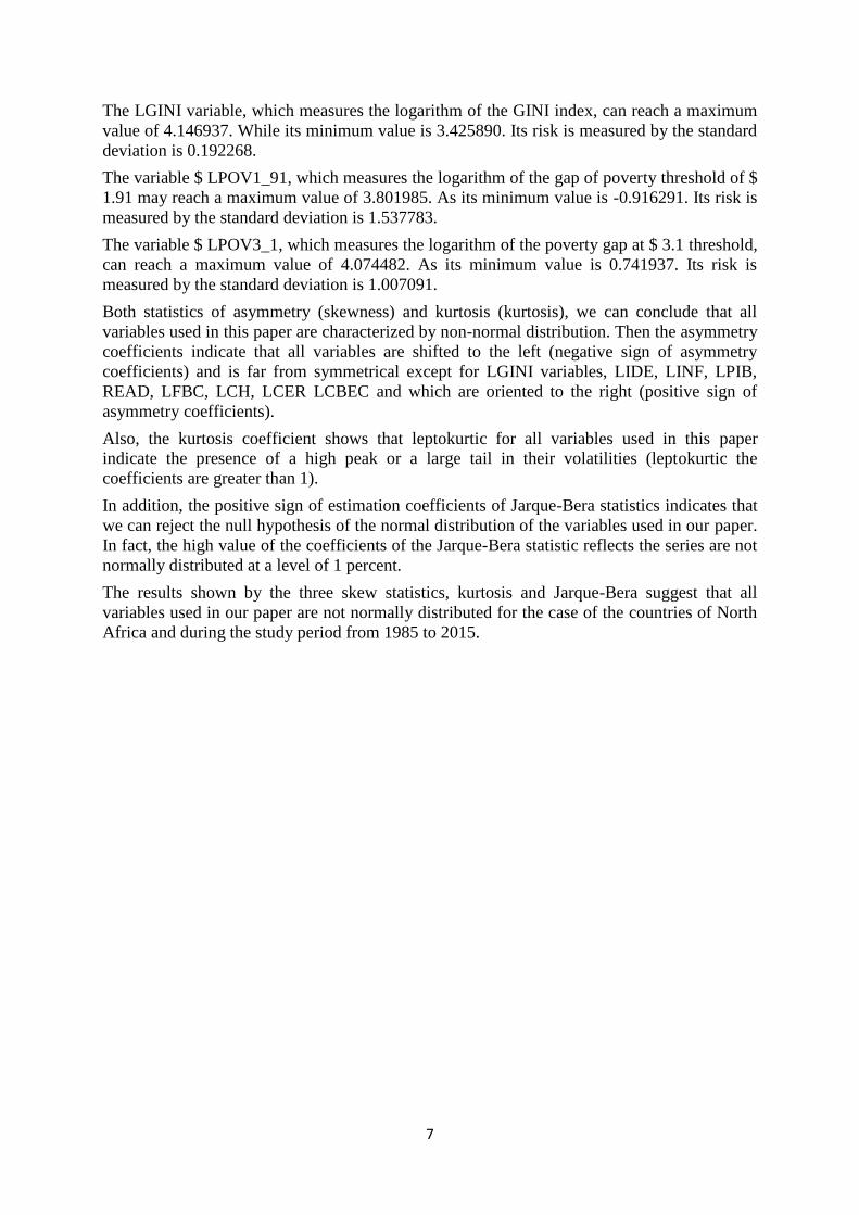
The LGINI variable, which measures the logarithm of the GINI index, can reach a maximum

value of 4.146937. While its minimum value is 3.425890. Its risk is measured by the standard

deviation is 0.192268.

The variable $ LPOV1_91, which measures the logarithm of the gap of poverty threshold of $

1.91 may reach a maximum value of 3.801985. As its minimum value is -0.916291. Its risk is

measured by the standard deviation is 1.537783.

The variable $ LPOV3_1, which measures the logarithm of the poverty gap at $ 3.1 threshold,

can reach a maximum value of 4.074482. As its minimum value is 0.741937. Its risk is

measured by the standard deviation is 1.007091.

Both statistics of asymmetry (skewness) and kurtosis (kurtosis), we can conclude that all

variables used in this paper are characterized by non-normal distribution. Then the asymmetry

coefficients indicate that all variables are shifted to the left (negative sign of asymmetry

coefficients) and is far from symmetrical except for LGINI variables, LIDE, LINF, LPIB,

READ, LFBC, LCH, LCER LCBEC and which are oriented to the right (positive sign of

asymmetry coefficients).

Also, the kurtosis coefficient shows that leptokurtic for all variables used in this paper

indicate the presence of a high peak or a large tail in their volatilities (leptokurtic the

coefficients are greater than 1).

In addition, the positive sign of estimation coefficients of Jarque-Bera statistics indicates that

we can reject the null hypothesis of the normal distribution of the variables used in our paper.

In fact, the high value of the coefficients of the Jarque-Bera statistic reflects the series are not

normally distributed at a level of 1 percent.

The results shown by the three skew statistics, kurtosis and Jarque-Bera suggest that all

variables used in our paper are not normally distributed for the case of the countries of North

Africa and during the study period from 1985 to 2015.

8

Table 3: Descriptive statistics LGINI $

LPOV1_91

$ LPOV3_1 LCO2 LIDE LINF LPIB LPU

Average 3.659430 1.711339 2.819903 10.52246 1.740903 12.13125 1.966823 3.953845

Median 3.572328 1.751173 2.913658 10.57184 1.226897 5.737290 1.894978 4.005441

Maximum 4.146937 3.801985 4.074482 12.30497 9.424248 132.8238 104.6576 4.361301

Minimum 3.425890 -0.916291 0.741937 7.975197 -0.469340 -9.797647 -62.21435 3.132751

Standard

Deviation

0.192268 1.537783 1.007091 1.022934 1.875266 21.34465 9.915128 0.299145

skewness 1.017615 -0.314673 -0.407684 -0.437984 1.658814 3.792586 4.340137 -0.572764

kurtosis 3.330697 1.869836 1.860567 2.615518 6.371119 18.51450 72.66292 2.511294

Jarque-Bera 32.94928 * 12.96843 * 15.21429 * 7.092390 * 173.3760 * 2311.317 * 38194.09 * 12.02076 *

Probability 0.000000 0.001527 0.000497 0.028834 0.000000 0.000000 0.000000 0.002453

Sum 680.6540 318.3091 524.5020 1957.178 323.8080 2256.413 365.8290 735.4151

Sum Sq. Dev. 6.838913 437.4836 187.6328 193.5830 650.5753 84284.89 18187.31 16.55519

observations 186 186 186 186 186 186 186 186

LTAJ LUE LDEP LDF LFBC CHL LCER LCBEC

Average 4.397266 4.647219 2.760326 3.117432 24.17608 2.671726 1.880000 3.329833

Median 4.400727 4.538225 3.187676 3.306042 24.53558 2.694627 2.356580 3.180049

Maximum 4.604464 5.460651 3.566570 4.336893 46.87646 3.394508 4.450014 5.622575

Minimum 4.067913 4.276705 1.401579 0.479664 4.329239 2.091864 -1.730354 0.716136

Standard

Deviation

0.148325 0.288363 0.742070 0.959663 7.523842 0.292898 1.737291 1.399367

skewness -0.428835 1.298344 -0.776126 -0.727663 0.207327 0.045106 -0.529717 -0.324575

kurtosis 2.526260 3.880495 1.924430 2.732941 3.446433 2.417982 2.494614 2.045393

Jarque-Bera 7.440210 ** 58.26498 * 27.63912 * 16.96701 * 200.877117 232.688345 10.67806 * 10.32820 *

Probability 0.024231 0.000000 0.000001 0.000207 0.000000 0.000000 0.004801 0.005718

Sum 817.8915 864.3827 513.4206 579.8423 4496.752 496.9410 349.6800 619.3490

Sum Sq. Dev. 4.070076 15.38337 101.8735 170.3764 10472.52 15.87098 558.3630 362.2723

observations 186 186 186 186 186 186 186 186

Thus, we conducted a test of the correlation between the different variables used in the case of the North African country during the study period

from 1985 to 2015. Table 4 summarizes the results for test Pearson correlation. In addition, the results showed that all coefficients between the explanatory variables do not exceed the tolerance limit (0.7), which does not

cause problems in the estimation of the model. That is to say, we can integrate the different variables used in the same model.

9

Table 4: The correlation matrix LGINI $

LPOV1_91

$ LPOV3_1 LCO2 LIDE LINF LPIB LPU

LGINI 1.000000 0.216744 0.154968 -0.165647 -0.220977 -0.227902 -0.017152 0.653434

$

LPOV1_91

0.216744 1.000000 0.089412 0.399300 -0.211419 0.025710 -0.059185 0.176666

$ LPOV3_1 0.154968 0.089412 1.000000 0.457670 -0.226173 0.013915 -0.057560 0.144844

LCO2 -0.165647 0.399300 0.457670 1.000000 0.000554 -0.472189 -0.028778 0.416057

LIDE -0.220977 -0.211419 -0.226173 0.000554 1.000000 -0.175203 0.107440 -0.116444

LINF -0.227902 0.025710 0.013915 -0.472189 -0.175203 1.000000 -0.034212 -0.550643

LPIB -0.017152 -0.059185 -0.057560 -0.028778 0.107440 -0.034212 1.000000 -0.022537

LPU 0.653434 0.176666 0.144844 0.416057 -0.116444 -0.550643 -0.022537 1.000000

LTAJ 0.526538 0.287783 0.208722 0.066702 0.093524 -0.139248 -0.014518 0.535036

LUE 0.274596 0.255015 0.194614 -0.655195 -0.074166 0.565342 -0.090298 -0.340264

LDEP -0.622753 -0.437272 -0.386163 0.404099 0.115025 -0.256776 -0.007249 0.011678

LDF 0.057127 -0.258985 -0.274410 0.330278 0.061514 -0.508943 -0.049271 0.390001

LFBC -0.167209 -0.192547 -0.163840 0.278071 0.174104 -0.297027 -0.008009 0.278378

CHL 0.478501 0.349806 0.310655 -0.192702 -0.311803 0.043348 -0.046815 0.281923

LCER -0.160403 -0.551713 -0.579122 -0.017235 0.273491 0.341804 0.070820 -0.627556

LCBEC -0.467603 -0.061890 0.025036 0.622213 -0.079906 -0.251845 -0.017867 0.102219

LTAJ LUE LDEP LDF LFBC CHL LCER LCBEC

GINI 0.526538 0.274596 -0.622753 0.057127 -0.167209 0.478501 -0.160403 -0.467603

$ POV1_91 0.287783 0.255015 -0.437272 -0.258985 -0.192547 0.349806 -0.551713 -0.061890

$ POV3_1 0.208722 0.194614 -0.386163 -0.274410 -0.163840 0.310655 -0.579122 0.025036

CO2 0.066702 -0.655195 0.404099 0.330278 0.278071 -0.192702 -0.017235 0.622213

FDI 0.093524 -0.074166 0.115025 0.061514 0.174104 -0.311803 0.273491 -0.079906

INF -0.139248 0.565342 -0.256776 -0.508943 -0.297027 0.043348 0.341804 -0.251845

GDP -0.014518 -0.090298 -0.007249 -0.049271 -0.008009 -0.046815 0.070820 -0.017867

COULD 0.535036 -0.340264 0.011678 0.390001 0.278378 0.281923 -0.627556 0.102219

TAJ 1.000000 0.287557 -0.393472 0.034387 -0.101385 0.309117 -0.278047 -0.444202

EU 0.287557 1.000000 -0.038724 -0.542902 -0.515000 0.271294 0.379276 -0.029952

DEP -0.393472 -0.038724 1.000000 0.538695 0.485806 -0.438228 -0.139890 0.011836

DF 0.034387 -0.542902 0.538695 1.000000 0.167907 -0.338843 -0.085541 0.181762

FBC -0.101385 -0.515000 0.485806 0.167907 1.000000 -0.180540 -0.400536 0.556466

CH 0.309117 0.271294 -0.438228 -0.338843 -0.180540 1.000000 -0.331089 -0.283439

RECs -0.278047 0.379276 -0.139890 -0.085541 -0.400536 -0.331089 1.000000 -0.489024

CBEC -0.444202 -0.029952 0.011836 0.181762 0.556466 -0.283439 -0.489024 1.000000

10

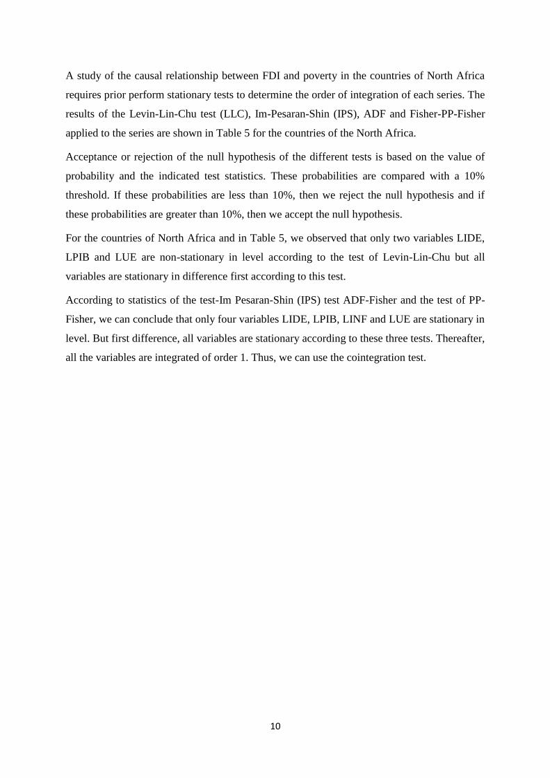
A study of the causal relationship between FDI and poverty in the countries of North Africa

requires prior perform stationary tests to determine the order of integration of each series. The

results of the Levin-Lin-Chu test (LLC), Im-Pesaran-Shin (IPS), ADF and Fisher-PP-Fisher

applied to the series are shown in Table 5 for the countries of the North Africa.

Acceptance or rejection of the null hypothesis of the different tests is based on the value of

probability and the indicated test statistics. These probabilities are compared with a 10%

threshold. If these probabilities are less than 10%, then we reject the null hypothesis and if

these probabilities are greater than 10%, then we accept the null hypothesis.

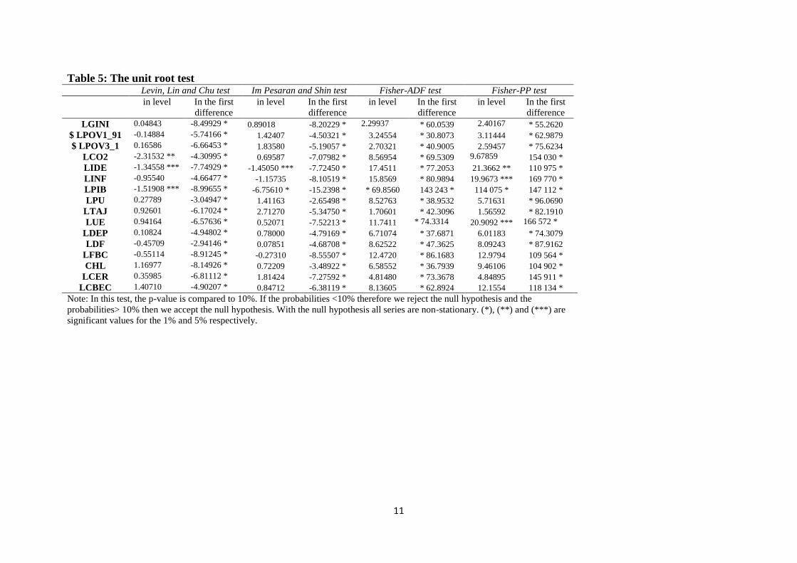
For the countries of North Africa and in Table 5, we observed that only two variables LIDE,

LPIB and LUE are non-stationary in level according to the test of Levin-Lin-Chu but all

variables are stationary in difference first according to this test.

According to statistics of the test-Im Pesaran-Shin (IPS) test ADF-Fisher and the test of PP-

Fisher, we can conclude that only four variables LIDE, LPIB, LINF and LUE are stationary in

level. But first difference, all variables are stationary according to these three tests. Thereafter,

all the variables are integrated of order 1. Thus, we can use the cointegration test.

11

Table 5: The unit root test Levin, Lin and Chu test Im Pesaran and Shin test Fisher-ADF test Fisher-PP test

in level In the first

difference


difference


difference


difference

LGINI 0.04843 -8.49929 * 0.89018 -8.20229 * 2.29937 * 60.0539 2.40167 * 55.2620

$ LPOV1_91 -0.14884 -5.74166 * 1.42407 -4.50321 * 3.24554 * 30.8073 3.11444 * 62.9879

$ LPOV3_1 0.16586 -6.66453 * 1.83580 -5.19057 * 2.70321 * 40.9005 2.59457 * 75.6234

LCO2 -2.31532 ** -4.30995 * 0.69587 -7.07982 * 8.56954 * 69.5309 9.67859 154 030 *

LIDE -1.34558 *** -7.74929 * -1.45050 *** -7.72450 * 17.4511 * 77.2053 21.3662 ** 110 975 *

LINF -0.95540 -4.66477 * -1.15735 -8.10519 * 15.8569 * 80.9894 19.9673 *** 169 770 *

LPIB -1.51908 *** -8.99655 * -6.75610 * -15.2398 * * 69.8560 143 243 * 114 075 * 147 112 *

LPU 0.27789 -3.04947 * 1.41163 -2.65498 * 8.52763 * 38.9532 5.71631 * 96.0690

LTAJ 0.92601 -6.17024 * 2.71270 -5.34750 * 1.70601 * 42.3096 1.56592 * 82.1910

LUE 0.94164 -6.57636 * 0.52071 -7.52213 * 11.7411 * 74.3314 20.9092 *** 166 572 *

LDEP 0.10824 -4.94802 * 0.78000 -4.79169 * 6.71074 * 37.6871 6.01183 * 74.3079

LDF -0.45709 -2.94146 * 0.07851 -4.68708 * 8.62522 * 47.3625 8.09243 * 87.9162

LFBC -0.55114 -8.91245 * -0.27310 -8.55507 * 12.4720 * 86.1683 12.9794 109 564 *

CHL 1.16977 -8.14926 * 0.72209 -3.48922 * 6.58552 * 36.7939 9.46106 104 902 *

LCER 0.35985 -6.81112 * 1.81424 -7.27592 * 4.81480 * 73.3678 4.84895 145 911 *

LCBEC 1.40710 -4.90207 * 0.84712 -6.38119 * 8.13605 * 62.8924 12.1554 118 134 *

Note: In this test, the p-value is compared to 10%. If the probabilities <10% therefore we reject the null hypothesis and the

probabilities> 10% then we accept the null hypothesis. With the null hypothesis all series are non-stationary. (*), (**) and (***) are

significant values for the 1% and 5% respectively.

12

5. Empirical Analysis

5.1. The cointegration test

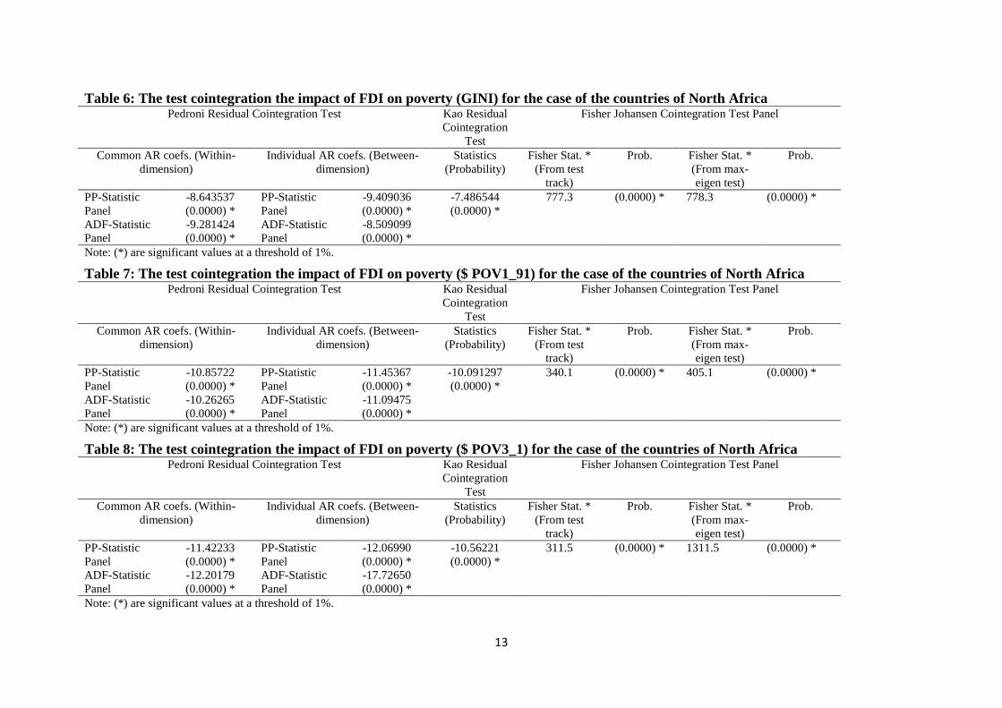
We will present in this part of the test results of cointegration. Kao tests, Pedroni and

Johenson Fisher cointegration are applied to ensure the long-term relationship between the

variables used in this paper to examine the impact of FDI on poverty for countries of North

Africa.

The Kao test is based on the statistical t-test and ADF Pedroni is based on two statistical

Panel and Panel-ADF-PP individual and grouped. But Fisher's test is based on the Fisher

statistical test track and Fisher Statistic of max-eigen test. The results of cointegration test for

the countries of North Africa are shown in Tables 6, 7 and 8.

Indeed, the Pedroni test demonstrates the long-term relationship between FDI and poverty

indicators. Thus, Kao test confirms the long term relationship between the different variables

used in our paper mainly between FDI and poverty indicators. In addition, Fisher's test results

confirm the presence of a long-term link between FDI and poverty in the countries of North

Africa for the study period from 1985 to 2015.

According to the results of the two tables 6, 7 and 8, we have certified the existence of a

cointegration relationship between the different series studied in our paper. Indeed, the result

of the null hypothesis test of no cointegration was rejected at the 5% threshold, which

explains the presence of a cointegration relationship. The results of these tests can determine

the use of an error correction model. Also, to test the effect of FDI on poverty in the countries

of North Africa, we will perform a FMOLS estimate.

13

Table 6: The test cointegration the impact of FDI on poverty (GINI) for the case of the countries of North Africa Pedroni Residual Cointegration Test Kao Residual

Cointegration

Test

Fisher Johansen Cointegration Test Panel

Common AR coefs. (Within-

dimension)

Individual AR coefs. (Between-

dimension)

Statistics

(Probability)

Fisher Stat. *

(From test

track)

Prob. Fisher Stat. *

(From max-

eigen test)

Prob.

PP-Statistic

Panel

ADF-Statistic

Panel

-8.643537

(0.0000) *

-9.281424

(0.0000) *

PP-Statistic

Panel

ADF-Statistic

Panel

-9.409036

(0.0000) *

-8.509099

(0.0000) *

-7.486544

(0.0000) *

777.3 (0.0000) * 778.3 (0.0000) *

Note: (*) are significant values at a threshold of 1%.

Table 7: The test cointegration the impact of FDI on poverty ($ POV1_91) for the case of the countries of North Africa Pedroni Residual Cointegration Test Kao Residual

Cointegration

Test



dimension)


dimension)

Statistics

(Probability)

Fisher Stat. *

(From test

track)


(From max-

eigen test)

Prob.

PP-Statistic

Panel

ADF-Statistic

Panel

-10.85722

(0.0000) *

-10.26265

(0.0000) *

PP-Statistic

Panel

ADF-Statistic

Panel

-11.45367

(0.0000) *

-11.09475

(0.0000) *

-10.091297

(0.0000) *

340.1 (0.0000) * 405.1 (0.0000) *


Table 8: The test cointegration the impact of FDI on poverty ($ POV3_1) for the case of the countries of North Africa Pedroni Residual Cointegration Test Kao Residual

Cointegration

Test



dimension)


dimension)

Statistics

(Probability)

Fisher Stat. *

(From test

track)


(From max-

eigen test)

Prob.

PP-Statistic

Panel

ADF-Statistic

Panel

-11.42233

(0.0000) *

-12.20179

(0.0000) *

PP-Statistic

Panel

ADF-Statistic

Panel

-12.06990

(0.0000) *

-17.72650

(0.0000) *

-10.56221

(0.0000) *

311.5 (0.0000) * 1311.5 (0.0000) *


14

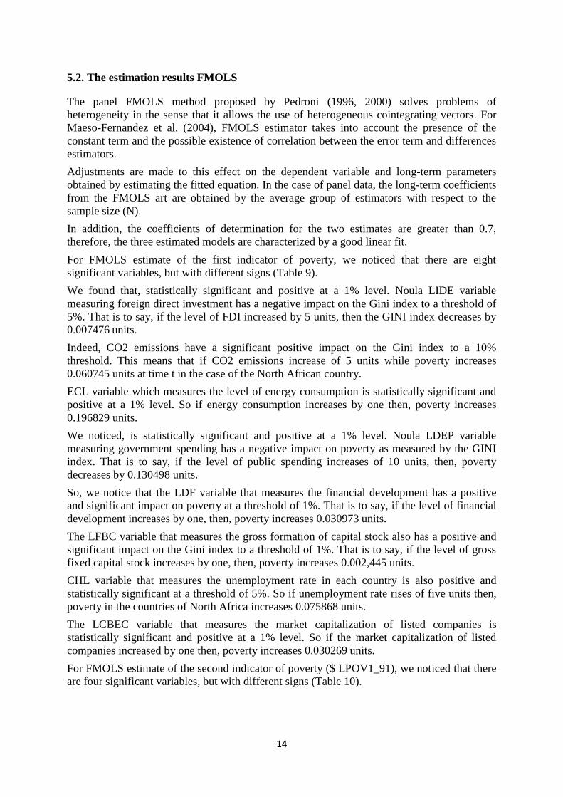
5.2. The estimation results FMOLS

The panel FMOLS method proposed by Pedroni (1996, 2000) solves problems of

heterogeneity in the sense that it allows the use of heterogeneous cointegrating vectors. For

Maeso-Fernandez et al. (2004), FMOLS estimator takes into account the presence of the

constant term and the possible existence of correlation between the error term and differences

estimators.

Adjustments are made to this effect on the dependent variable and long-term parameters

obtained by estimating the fitted equation. In the case of panel data, the long-term coefficients

from the FMOLS art are obtained by the average group of estimators with respect to the

sample size (N).

In addition, the coefficients of determination for the two estimates are greater than 0.7,

therefore, the three estimated models are characterized by a good linear fit.

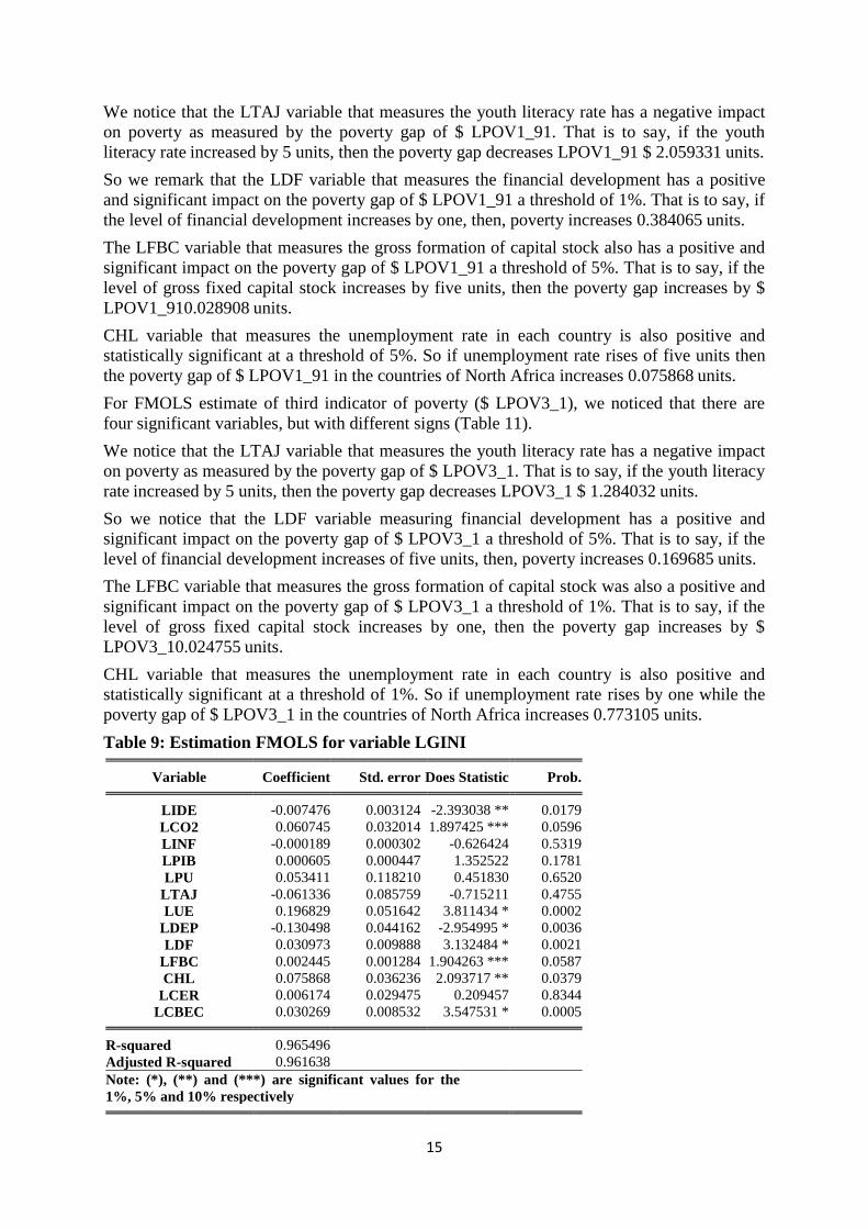
For FMOLS estimate of the first indicator of poverty, we noticed that there are eight

significant variables, but with different signs (Table 9).

We found that, statistically significant and positive at a 1% level. Noula LIDE variable

measuring foreign direct investment has a negative impact on the Gini index to a threshold of

5%. That is to say, if the level of FDI increased by 5 units, then the GINI index decreases by

0.007476 units.

Indeed, CO2 emissions have a significant positive impact on the Gini index to a 10%

threshold. This means that if CO2 emissions increase of 5 units while poverty increases

0.060745 units at time t in the case of the North African country.

ECL variable which measures the level of energy consumption is statistically significant and

positive at a 1% level. So if energy consumption increases by one then, poverty increases

0.196829 units.

We noticed, is statistically significant and positive at a 1% level. Noula LDEP variable

measuring government spending has a negative impact on poverty as measured by the GINI

index. That is to say, if the level of public spending increases of 10 units, then, poverty

decreases by 0.130498 units.

So, we notice that the LDF variable that measures the financial development has a positive

and significant impact on poverty at a threshold of 1%. That is to say, if the level of financial

development increases by one, then, poverty increases 0.030973 units.

The LFBC variable that measures the gross formation of capital stock also has a positive and

significant impact on the Gini index to a threshold of 1%. That is to say, if the level of gross

fixed capital stock increases by one, then, poverty increases 0.002,445 units.

CHL variable that measures the unemployment rate in each country is also positive and

statistically significant at a threshold of 5%. So if unemployment rate rises of five units then,

poverty in the countries of North Africa increases 0.075868 units.

The LCBEC variable that measures the market capitalization of listed companies is

statistically significant and positive at a 1% level. So if the market capitalization of listed

companies increased by one then, poverty increases 0.030269 units.

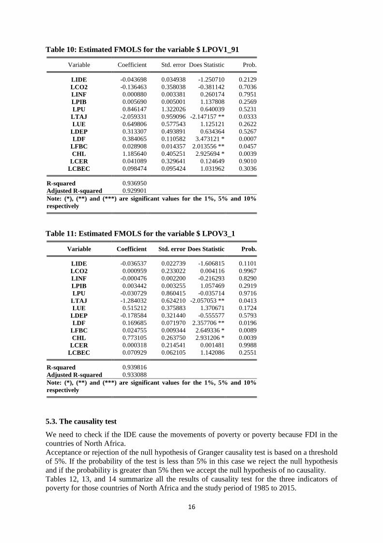
For FMOLS estimate of the second indicator of poverty ($ LPOV1_91), we noticed that there

are four significant variables, but with different signs (Table 10).

15

We notice that the LTAJ variable that measures the youth literacy rate has a negative impact

on poverty as measured by the poverty gap of $ LPOV1_91. That is to say, if the youth

literacy rate increased by 5 units, then the poverty gap decreases LPOV1_91 $ 2.059331 units.

So we remark that the LDF variable that measures the financial development has a positive

and significant impact on the poverty gap of $ LPOV1_91 a threshold of 1%. That is to say, if

the level of financial development increases by one, then, poverty increases 0.384065 units.

The LFBC variable that measures the gross formation of capital stock also has a positive and

significant impact on the poverty gap of $ LPOV1_91 a threshold of 5%. That is to say, if the

level of gross fixed capital stock increases by five units, then the poverty gap increases by $

LPOV1_910.028908 units.


statistically significant at a threshold of 5%. So if unemployment rate rises of five units then

the poverty gap of $ LPOV1_91 in the countries of North Africa increases 0.075868 units.

For FMOLS estimate of third indicator of poverty ($ LPOV3_1), we noticed that there are

four significant variables, but with different signs (Table 11).

We notice that the LTAJ variable that measures the youth literacy rate has a negative impact

on poverty as measured by the poverty gap of $ LPOV3_1. That is to say, if the youth literacy

rate increased by 5 units, then the poverty gap decreases LPOV3_1 $ 1.284032 units.

So we notice that the LDF variable measuring financial development has a positive and


level of financial development increases of five units, then, poverty increases 0.169685 units.

The LFBC variable that measures the gross formation of capital stock was also a positive and


level of gross fixed capital stock increases by one, then the poverty gap increases by $

LPOV3_10.024755 units.


statistically significant at a threshold of 1%. So if unemployment rate rises by one while the

poverty gap of $ LPOV3_1 in the countries of North Africa increases 0.773105 units.

Table 9: Estimation FMOLS for variable LGINI Variable Coefficient Std. error Does Statistic Prob.

LIDE -0.007476 0.003124 -2.393038 ** 0.0179

LCO2 0.060745 0.032014 1.897425 *** 0.0596

LINF -0.000189 0.000302 -0.626424 0.5319

LPIB 0.000605 0.000447 1.352522 0.1781

LPU 0.053411 0.118210 0.451830 0.6520

LTAJ -0.061336 0.085759 -0.715211 0.4755

LUE 0.196829 0.051642 3.811434 * 0.0002

LDEP -0.130498 0.044162 -2.954995 * 0.0036

LDF 0.030973 0.009888 3.132484 * 0.0021

LFBC 0.002445 0.001284 1.904263 *** 0.0587

CHL 0.075868 0.036236 2.093717 ** 0.0379

LCER 0.006174 0.029475 0.209457 0.8344

LCBEC 0.030269 0.008532 3.547531 * 0.0005

R-squared 0.965496

Adjusted R-squared 0.961638

Note: (*), (**) and (***) are significant values for the

1%, 5% and 10% respectively

16

Table 10: Estimated FMOLS for the variable $ LPOV1_91 Variable Coefficient Std. error Does Statistic Prob.

LIDE -0.043698 0.034938 -1.250710 0.2129

LCO2 -0.136463 0.358038 -0.381142 0.7036

LINF 0.000880 0.003381 0.260174 0.7951

LPIB 0.005690 0.005001 1.137808 0.2569

LPU 0.846147 1.322026 0.640039 0.5231

LTAJ -2.059331 0.959096 -2.147157 ** 0.0333

LUE 0.649806 0.577543 1.125121 0.2622

LDEP 0.313307 0.493891 0.634364 0.5267

LDF 0.384065 0.110582 3.473121 * 0.0007

LFBC 0.028908 0.014357 2.013556 ** 0.0457

CHL 1.185640 0.405251 2.925694 * 0.0039

LCER 0.041089 0.329641 0.124649 0.9010

LCBEC 0.098474 0.095424 1.031962 0.3036

R-squared 0.936950


Note: (*), (**) and (***) are significant values for the 1%, 5% and 10%

respectively

Table 11: Estimated FMOLS for the variable $ LPOV3_1 Variable Coefficient Std. error Does Statistic Prob.

LIDE -0.036537 0.022739 -1.606815 0.1101

LCO2 0.000959 0.233022 0.004116 0.9967

LINF -0.000476 0.002200 -0.216293 0.8290

LPIB 0.003442 0.003255 1.057469 0.2919

LPU -0.030729 0.860415 -0.035714 0.9716

LTAJ -1.284032 0.624210 -2.057053 ** 0.0413

LUE 0.515212 0.375883 1.370671 0.1724

LDEP -0.178584 0.321440 -0.555577 0.5793

LDF 0.169685 0.071970 2.357706 ** 0.0196

LFBC 0.024755 0.009344 2.649336 * 0.0089

CHL 0.773105 0.263750 2.931206 * 0.0039

LCER 0.000318 0.214541 0.001481 0.9988

LCBEC 0.070929 0.062105 1.142086 0.2551

R-squared 0.939816


Note: (*), (**) and (***) are significant values for the 1%, 5% and 10%

respectively

5.3. The causality test

We need to check if the IDE cause the movements of poverty or poverty because FDI in the

countries of North Africa.

Acceptance or rejection of the null hypothesis of Granger causality test is based on a threshold

of 5%. If the probability of the test is less than 5% in this case we reject the null hypothesis

and if the probability is greater than 5% then we accept the null hypothesis of no causality.

Tables 12, 13, and 14 summarize all the results of causality test for the three indicators of

poverty for those countries of North Africa and the study period of 1985 to 2015.

17

According to Table 12, we noticed that there is a unidirectional relationship between the

consumption of energy and poverty Granger (0.9956> 0.0102 and 5% <5%). Only the GINI

index can cause Granger consumption of energy.

Thus there is no causal relationship between the Gini index and other senses to control

variables Granger as their probability values are greater than 0.05, which allow accepting the

null hypothesis of the test.

According to Table 13, we noticed that there is no causal relationship between poverty gap to

$ 1.91 and the other control variables Granger as their probability values are greater than 0.05,

which allow accepting the null hypothesis of the test.

According to Table 14, we noticed that there is no causal relationship between poverty gap of

$ 3.1 and other control variables Granger as their probability values are greater than 0.05,

which allow accepting the null hypothesis of the test.

Table 12: The causality test for variable LGINI Null Hypothesis: Obs F-Statistic Prob.

CO2 does not Granger Cause GINI 174 0.02150 0.9787

GINI does not Granger Cause CO2 2.05242 0.1316

FDI does not Granger Cause GINI 174 0.06502 0.9371

GINI does not Granger Cause IDE 1.40501 0.2482

INF does not Granger Cause GINI 174 0.16511 0.8479

GINI does not Granger Cause INF 0.22829 0.7961

GDP does not Granger Cause GINI 174 0.05708 0.9445

GINI does not Granger Cause GDP 1.45896 0.2354

PU does not Granger Cause GINI 174 0.00394 0.9961

GINI does not Granger Cause PU 0.01741 0.9827

TAJ does not Granger Cause GINI 174 0.71878 0.4888

GINI does not Granger Cause TAJ 0.02269 0.9776

EU does not Granger Cause GINI 174 0.00440 0.9956

GINI does not Granger Cause EU 4.70942 0.0102

DEP does not Granger Cause GINI 174 0.92156 0.3999

GINI does not Granger Cause DEP 0.07589 0.9270

DF does not Granger Cause GINI 174 0.30542 0.7372

GINI does not Granger Cause DF 0.92725 0.3976

BCF does not Granger Cause GINI 174 0.41309 0.6623

GINI does not Granger Cause FBC 1.46845 0.2332

CH does not Granger Cause Gini 174 0.03707 0.9636

Gini does not Granger Cause CH 0.59528 0.5526

REC does not Granger Cause GINI 174 0.30342 0.7387

GINI does not Granger Cause CER 0.30986 0.7340

CBEC does not Granger Cause GINI 174 0.87943 0.4169

GINI does not Granger Cause CBEC 0.58106 0.5604

18

Table 13: The causality test for the variable $ LPOV1_91 Null Hypothesis: Obs F-Statistic Prob.

CO2 does not Granger Cause $ POV1_91 174 0.29971 0.7414

$ POV1_91 does not Granger Cause CO2 0.41057 0.6639

FDI does not Granger Cause $ POV1_91 174 0.83992 0.4335

$ POV1_91 does not Granger Cause IDE 2.24868 0.1087

INF does not Granger Cause $ POV1_91 174 0.20629 0.8138

$ POV1_91 does not Granger Cause INF 0.11658 0.8900

GDP does not Granger Cause $ POV1_91 174 0.25314 0.7767

$ POV1_91 does not Granger Cause GDP 1.04794 0.3529

PU does not Granger Cause $ POV1_91 174 0.21266 0.8086

$ POV1_91 does not Granger Cause PU 0.12238 0.8849

TAJ does not Granger Cause $ POV1_91 174 0.18553 0.8308

$ POV1_91 does not Granger Cause TAJ 0.76788 0.4656

EU does not Granger Cause $ POV1_91 174 0.71114 0.4925

$ POV1_91 does not Granger Cause EU 0.70694 0.4946

DEP does not Granger Cause $ POV1_91 174 2.11998 0.1232

$ POV1_91 does not Granger Cause DEP 0.92243 0.3995

DF does not Granger Cause $ POV1_91 174 1.07477 0.3437

$ POV1_91 does not Granger Cause DF 1.78316 0.1713

BCF does not Granger Cause $ POV1_91 174 0.09534 0.9091

$ POV1_91 does not Granger Cause FBC 0.23879 0.7878

CH does not Granger Cause $ POV1_91 174 0.40424 0.6681

$ POV1_91 does not Granger Cause CH 0.42171 0.6566

REC does not Granger Cause $ POV1_91 174 0.00168 0.9983

$ POV1_91 does not Granger Cause CER 0.83364 0.4362

CBEC does not Granger Cause $ POV1_91 174 0.10968 0.8962

$ POV1_91 does not Granger Cause CBEC 0.06561 0.9365

Table 14: The causality test for the variable $ LPOV3_1 Null Hypothesis: Obs F-Statistic Prob.

CO2 does not Granger Cause $ POV3_1 174 0.27003 0.7637

$ POV3_1 does not Granger Cause CO2 0.25712 0.7736

FDI does not Granger Cause $ POV3_1 174 1.02480 0.3611

$ POV3_1 does not Granger Cause IDE 2.79780 0.0638

INF does not Granger Cause $ POV3_1 174 0.33738 0.7141

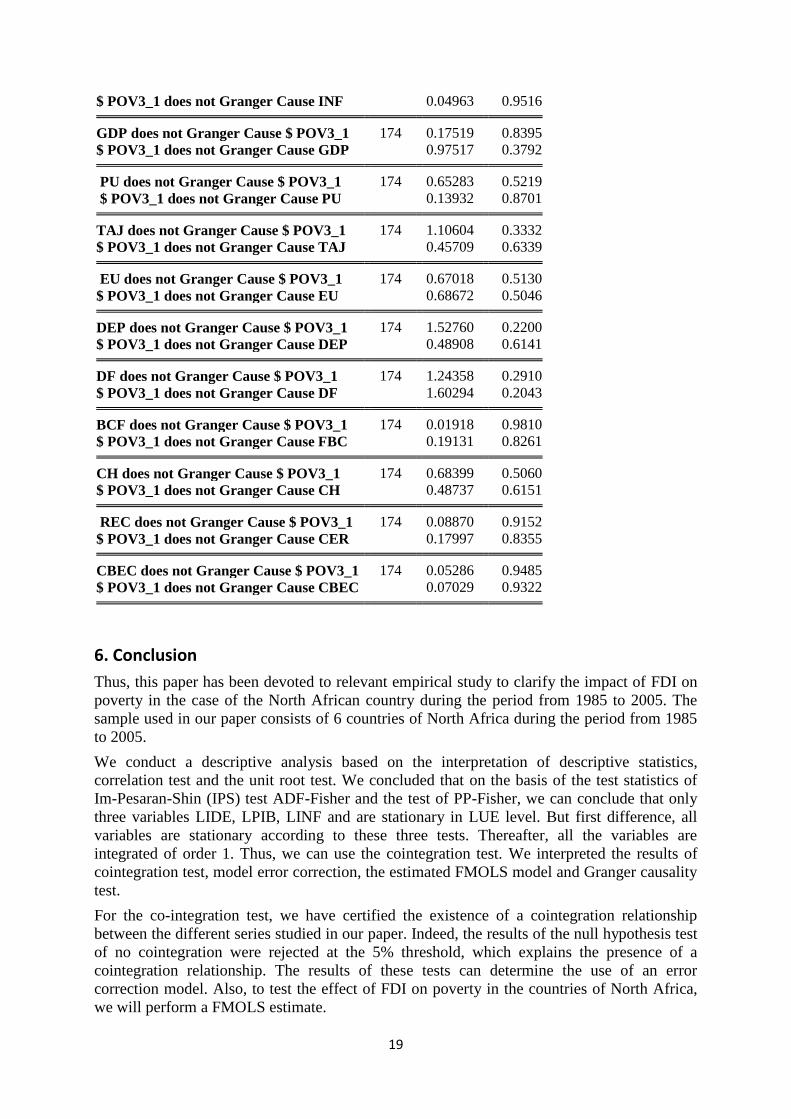
19

$ POV3_1 does not Granger Cause INF 0.04963 0.9516

GDP does not Granger Cause $ POV3_1 174 0.17519 0.8395

$ POV3_1 does not Granger Cause GDP 0.97517 0.3792

PU does not Granger Cause $ POV3_1 174 0.65283 0.5219

$ POV3_1 does not Granger Cause PU 0.13932 0.8701

TAJ does not Granger Cause $ POV3_1 174 1.10604 0.3332

$ POV3_1 does not Granger Cause TAJ 0.45709 0.6339

EU does not Granger Cause $ POV3_1 174 0.67018 0.5130

$ POV3_1 does not Granger Cause EU 0.68672 0.5046

DEP does not Granger Cause $ POV3_1 174 1.52760 0.2200

$ POV3_1 does not Granger Cause DEP 0.48908 0.6141

DF does not Granger Cause $ POV3_1 174 1.24358 0.2910

$ POV3_1 does not Granger Cause DF 1.60294 0.2043

BCF does not Granger Cause $ POV3_1 174 0.01918 0.9810

$ POV3_1 does not Granger Cause FBC 0.19131 0.8261

CH does not Granger Cause $ POV3_1 174 0.68399 0.5060

$ POV3_1 does not Granger Cause CH 0.48737 0.6151

REC does not Granger Cause $ POV3_1 174 0.08870 0.9152

$ POV3_1 does not Granger Cause CER 0.17997 0.8355

CBEC does not Granger Cause $ POV3_1 174 0.05286 0.9485

$ POV3_1 does not Granger Cause CBEC 0.07029 0.9322

6. Conclusion

Thus, this paper has been devoted to relevant empirical study to clarify the impact of FDI on

poverty in the case of the North African country during the period from 1985 to 2005. The

sample used in our paper consists of 6 countries of North Africa during the period from 1985

to 2005.

We conduct a descriptive analysis based on the interpretation of descriptive statistics,

correlation test and the unit root test. We concluded that on the basis of the test statistics of

Im-Pesaran-Shin (IPS) test ADF-Fisher and the test of PP-Fisher, we can conclude that only

three variables LIDE, LPIB, LINF and are stationary in LUE level. But first difference, all

variables are stationary according to these three tests. Thereafter, all the variables are

integrated of order 1. Thus, we can use the cointegration test. We interpreted the results of

cointegration test, model error correction, the estimated FMOLS model and Granger causality

test.

For the co-integration test, we have certified the existence of a cointegration relationship

between the different series studied in our paper. Indeed, the results of the null hypothesis test

of no cointegration were rejected at the 5% threshold, which explains the presence of a

cointegration relationship. The results of these tests can determine the use of an error

correction model. Also, to test the effect of FDI on poverty in the countries of North Africa,

we will perform a FMOLS estimate.

20

Thus, for the short-term dynamics, we noticed that FDI have a positive and significant impact

on a threshold of 1% on the GINI index for the case of the countries of North Africa and a

significant negative a threshold of 1% for the other two indicators of poverty; LPOV1_91 $

and LPOV3_1 $.

Then we found that the LIDE variable measuring foreign direct investment has a negative

impact on the Gini index to a threshold of 5%. That is to say, if the level of FDI increased by

5 units, then the GINI index decreases by 0.007476 units.

Finally, Granger causality test, we noticed that there is a unidirectional relationship between

the consumption of energy and poverty Granger. Only the GINI index can cause Granger

consumption of energy.

References

Sumner A. (2005), Is foreign direct investment good for the poor? A review and stocktake,

ʻDevelopment in Practiceʼ, no. 15 ( 3/4).

Meyer K.E. (2004), Perspectives on Multinational enterprises in emerging economies,

ʻJournal of International Business Studiesʼ, no. 35(4).

Gorg H. and Greenaway D. (2004), Much ado about nothing? Do domestic firms really

benefit from foreign direct investment? ʻThe World Bank Research Observerʼ, no.

19(2).

Hung T.T. (1999), Impact of Foreign Direct Investment on Poverty Reduction in Vietnam,

IDS Program, GRIPS.

Jalilian H. and Weiss J. (2002), Foreign direct investment and poverty in the ASEAN region,

ʻASEAN Economic Bulletinʼ, no. 19(3).

Calvo C.C. and Hernandez M.A. (2006), Foreign direct investment and poverty in Latin

America, Leverhulme Centre for Research on Globalisation and Economic Policy,

University of Nottingham.

Reiter S.L. and Steensma H.K. (2010), Human development and foreign direct investment in

developing countries: the influence of foreign direct investment policy and corruption,

ʻWorld Development,ʼ no. 38 (12).

Zaman K.. Khan M.M. and Ahmad M. (2012), The relationship between foreign direct

investment and pro-poor growth policies in Pakistan: The new interface, ʻEconomic

Modellingʼ no. 29.

Mahmood H. and Chaudhary A.R. (2012), A contribution of foreign direct investment in

poverty reduction in Pakistan, ʻMiddle East Journal of Scientific Researchʼ no. 12(2).

Fowowe B. and Shuaibu M.I. (2014), Is foreign direct investment good for the poor? New

evidence from African Countries. ʻEco Change Restructʼ, no. 47.

Shamim A., Azeem P. and Naqvi M.A. (2014), Impact of foreign direct investment on

poverty reduction in Pakistan, ʻInternational Journal of Academic Research in

Business and Social Sciencesʼ, no 4(10).

Ucal M.S. (2014), Panel data analysis of foreign direct investment and poverty from the

perspective of developing countries, ʻSocial and Behavioral Scienceʼ, no. 109.

21

Bharadwaj A. (2014), Reviving the globalisation and poverty debate: Effects of real and

financial integration on the developing world, ʻAdvances in Economics and Businessʼ

no. 2(1).

Uttama N.P., (2015), Foreign Direct Investment and Poverty Reduction Nexus in South East

Asia, [in:] Silber J. Poverty Reduction Policies and Practices in Developing Asia

Im, H., McLaren, J. (2015) “Does Foreign Direct Investment Raise Income Inequality in

Developing Countries? A New Instrumental Variables Approach”, retrieved from

https://www.rse.anu.edu.au/media/772451/Im-Hyejoon.pdf

Documents

The impact of FDI on Poverty Reduction in North Africa