The Impact of Consumer’s Bounded Rationality on Retailer’s

Price and Location Decisions

Tom Blockmans a∗, Frank Plastria a , Lieselot Vanhaverbeke a

aDepartment MOSI (Mathematics, OR, Statistics and IS for Management)Vrije Universiteit Brussel

Pleinlaan 2, 1050 Brussels, Belgium

Abstract

As is the case with most OR models, the original maximal covering location problemwith price decision (PrMAXCOV) assumes perfect rationality on the part of the consumer.This is clearly contradicted by the evidence found in marketing literature. Starting fromthis experimental evidence, we illustrate through the PrMAXCOV how these mathemat-ical models can be adapted in order to better reflect the consumer’s bounded rationalitythat appears in real life.

First, we examine the impact of rounded pricing on the solution of the model. Ourresults show that simply rounding the solution of a given problem may not always beadvisable. In some cases it is advantageous to restrict the possible solutions to roundedvalues in advance. Based on the rounded optimal solution, we show that expected revenueis actually an underestimation due to the drop-off mechanism. Secondly, we illustrate thatwhen retailers limit their prices to predetermined ranges, this will almost always result ina loss of revenue. Finally, we show that when the model considers the fact that certaincustomers pay little attention to the price, firms will generally charge higher prices andlocate closer to these inattentive and/or uninformed customers.

Keywords: Location, Marketing, Pricing, Decision making

∗Corresponding author. Tel.: +3226292068; Fax: +3226293690; email address: Tom.Blockmans@vub.ac.be

1

1 Introduction

When entering a competitive market, a firm has to make several crucial choices. These deci-sions relate to all possible aspects of the enterprise and the products it provides. Combined,these decisions make up the firm’s strategy towards achieving its objectives. In most compa-nies, this means maximizing shareholder value and/or profits.

In marketing literature, the firm’s strategic decisions are generally grouped into four cat-egories, commonly known as the four P’s: product, price, place and promotion. In each ofthese categories a firm must position itself vis-a-vis the competition. The model used in thisarticle assumes the product to be homogeneous, thus ruling out any differentiation withinthat category of the marketing mix. We also ignore promotional activities. This leaves twoimportant factors to be determined, namely place (location) and price.

When deciding on location and pricing strategy, it is important for a firm to considerthe manner in which consumers will react to them. This will, for a large part, depend onthe decision making process employed by these consumers. Most significantly, a firm mustdetermine what information is used by its customers and how this information is processed.

Most models within the field of locational analysis assume that the customers are fullyinformed and perfectly rational. For a detailed overview of consumer behavior modeling, seeVanhaverbeke [1]. This means that they do not only have access to all the necessary infor-mation, they also process it in a fully rational manner. However, empirical evidence suggeststhat “consumer rationality is a property of the researcher’s model rather than the consumer”[2].

As a solution towards reducing the discrepancy between consumer behavior in locationanalysis models and the behavior as it is described in marketing literature, we propose toimplement some degree of bounded rationality. Simon [3], who coined the phrase of boundedrationality, extended the “rational choice theory by including decision-makers that have lim-ited knowledge and finite cognitive abilities”. In doing so, he “discards the assumption thatcustomers have perfect information and, for that matter, neither have the information theyneed nor know what information they need” [4].

To illustrate the impact that bounded rationality on the consumer’s part can have on aretailer’s location and price decisions, a model is required in which the optimal choices forboth these variables are decided upon by the retailer. Formal models with the sole objectiveof determining a firm’s optimal location “have been studied in various forms for hundreds ofyears” [5]. Their emergence is most often linked with the seminal paper titled “Stability inCompetition” [6]. In that article Hotelling established the “Principle of Minimal Differentia-tion” for a duopoly on a linear market, proving that in equilibrium both firms will locate atthe middle of the market. This result was later shown to be a consequence of the stringentassumption used in the model. D’Aspremont et al. [7] even found the opposite result whenslightly altering the assumptions of the original model. Nevertheless, he “set the foundations

2

of what is today the burgeoning field of competitive location” [8]. An overview of recent workwithin the broad field of locational analysis has been assembled by ReVelle et al. [5].

However, most of these competitive location models did not attribute the retailer withthe ability to determine a preferred price level. An initial price-location model was developedby Serra and ReVelle [8], who extended the maximum capture model [9] with a price decision,using a heuristic method to solve the problem. An alternative approach has been presented byPlastria and Vanhaverbeke [10]. Their maximal covering location problem with price decision(PrMAXCOV) determines the optimal location of the firm’s outlets and the price that mustbe charged in order to generate maximal revenue. Contrary to Serra and ReVelle [8], theypresented an exact solution method.

The PrMAXCOV model will be used here to illustrate the effects that consumer’s boundedrationality can have on the retailer’s price and location decisions. The model and the solutionmethods as developed by Plastria and Vanhaverbeke will be presented in section 2. This isfollowed by a comparison between the consumer behavior as it was assumed in the modeland the behavior that is described in marketing literature, based on empirical evidence. Inan attempt to lessen the difference between these two approaches, we formulate some con-sumer inspired variations to the model in section 3 and examine their impact on the optimalprice levels, outlet locations and the retailer’s revenue. These will be complemented by twopractical restrictions that retailer may be faced with and which also may have considerable in-fluence on the retailer’s price and location decisions. Some concluding remarks are presentedin section 4.

2 Consumer rationality in the PrMAXCOV

The PrMAXCOV by Plastria and Vanhaverbeke [10] determines the optimal locations andoptimal price for a firm that is entering a market where competitors are already present.The decisions regarding location of outlets and price level made by the firm are based on thebehavior that consumers are assumed to display. As is the case for most models within thefield of locational analysis, this behavior is regarded as perfectly rational and fully informed.

When a firm is a wholesaler, perfect rationality can be a reasonable assumption withregard to its customers. A wholesale company supplies other companies, who often employprofessional buyers. These purchasers (aim to) use all the information available to themand often use tools to process this information, such as spreadsheets. This enables them tomake fully informed and rational decisions. However, retail consumer behavior is often notas rational as assumed in most models. Among the most common explanations are boundedrationality and imperfect information. This raises the question on how consumer behavior asperceived in marketing literature relates to the behavior as modeled in locational analysis.A comparison between these two approaches is the subject of this section, illustrated by the

3

PrMAXCOV.

2.1 The model

Extending the classic Maximal Covering Location Problem by Church and ReVelle [11] witha price decision, Plastria and Vanhaverbeke chose to employ to a large extent the samenotations. A firm entering a competitive market will locate a fixed, predetermined numberof outlets at a finite number of locations (set J), given the fixed locations of the competingstores (set C). As both the classic maximal covering model and the PrMAXCOV are discretemodels, customers (set I) are represented by demand points. As mentioned by the authors,these points are often the result of an aggregation process done beforehand, as described inan earlier article [12]. For a survey on aggregation methods and errors in location models,see Francis et al. [13].

Besides the obvious difference in objective functions, there is one important point ofcontrast between the revenue maximizing model and the classic model. Church and ReVelle[11] maximize the covered demand, with the added restriction that “no demand point willbe farther than the maximal service distance from a facility”. This reflects the fact that,for inessential goods, consumers will only travel a predetermined maximal distance (dmax) inorder to make a purchase. Plastria and Vanhaverbeke consider the case of essential goods, who“will always be purchased, no matter how far the customer must travel to acquire the good”[10]. The possibility of introducing dmax in their model is mentioned, but not implemented.

The objective of the PrMAXCOV is to maximize revenue, rather than covered demand.This is achieved by introducing the mill price (p) in the objective function of the model,shown in equation (1), and multiplying it with the demand covered.∏∗

= max∑i∈I

qixip (1)

The covered demand is determined by multiplying the amount of demand represented byeach customer (qi) by a “covering variable (xi), taking the value 1 when the customer i iscovered by at least one of the outlets of the new firm or remains 0 if not” [10].

Customers will not make their buying decision based only on the mill price at the outlet,but rather on the total purchasing cost. This total cost is composed of the “price p chargedby the new player and the transportation cost (t) over the distance (dij) traveled by customeri to outlet j ” [10]. Customers are assumed to show novelty behavior, which implies that “incase of a tie, the new facility gets all demand” [14]. A tie can occur when, by accident, acustomer’s total purchasing cost is equal for the existing and the new player. Plastria andVanhaverbeke [10] subsequently defined that “customer i will patronize a facility j ∈ J if thesum of the price charged by the existing players plus his transportation cost to the existing

4

player’s closest outlet is strictly higher than the total price at the new outlet” [10]. All thisis stated in the following inequality:

p + tdij ≤ minc∈C

(pc + tdic) ∀i ∈ I, j ∈ J (2)

This leads to the definition of the so-called critical price: “the minimum of the total pricesof all existing player outlets for customer i, minus the transportation costs for the distancefrom customer i to the new outlet j ” [10]. This is called the critical price because if the pricep charged by the new firm undercuts pij , customer i will patronize a new outlet at j.

pij = minc∈C

(pc + tdic)− tdij ∀i ∈ I, j ∈ J (3)

Based on the critical price, Plastria and Vanhaverbeke [10] also defined the patronizing setNi(p) as “containing all facilities for which the critical price pij is at least p”:

Ni(p) = {j ∈ J : pij ≥ p} ∀i ∈ I (4)

The following mathematical formulation of the complete model was defined:

max∑i∈I

qixip (5)

s.t.∑

j∈Ni(p)

yj ≥ xi ∀i ∈ I (6)∑j∈J

yj = B (7)

0 ≤ xi ≤ 1 ∀i ∈ I (8)

yj ∈ {0, 1} ∀j ∈ J (9)

p ≥ pmin (10)

Equation (5) is the objective function, which was already analyzed above. Equation (6)expresses the so-called covering constraint. It defines that “at least one facility in the setNi(p) must be opened for customer i to be covered by the new firm, under price setting p”[10]. The location variable (yj) takes value 1 if a new outlet is opened at location j and 0otherwise, which is defined in equation (9).

One could expect the definition of the covering variable (xi) in equation (8) to have asimilar expression as the location variable (yj). Unlike the location variable, the coveringvariable is not restricted to binary values, but rather “continuous and bounded between 0and 1” [15]. This is due to the fact that the optimization process will push the variable to itsextreme values 0 or 1. From equation (9) it can be deduced that the constraining values inthe covering constraint (6) will either be 0 or at least 1. As the covering variable is part of the

5

objective function it will always be maximized, resulting in a de facto binary value. In prac-tice it appears that when using commercial software “any reduction in the number of binaryvariables may allow to increase the problem size without reaching the limits of tractability”[15].

Equation (7) expresses the budget constraint. “A new firm is limited to a number B ofnew facilities to open” [10]. This can be easily modified into a monetary budget constraintif a fixed cost in attributed to each facility. Finally, a minimum price is defined in equation(10), which may not be undercut. It expresses the fact that costs must be covered by theprice and “operating with loss is not allowed” [10]. Plastria and Vanhaverbeke assumed thatall firms have the same cost structure, which allowed them to make abstraction of the variablecost. The advantage of using this assumption is that, given the identical cost structure of alloutlets, revenue maximization corresponds to profit maximization.

As mentioned in the introductory section, Plastria and Vanhaverbeke have developedan exact solution method for determining the maximal revenue for the PrMAXCOV. Theydeclare in their paper: “this problem is a special case of the heuristically solved problem“PMAXCAP” by Serra and ReVelle” [10]. The difference lies in the fact that, unlike Serraand ReVelle, they do not take into account demand elasticity.

The solution method was developed in two main steps. First, they determine a full enu-meration method, which is only applicable for small size problems due to the limited capacityof commercially available software. This is followed by an intelligent enumeration method,using “some characteristics of the covering problem to help narrow down the solution spaceand avoid full enumeration” [10].

Starting with the full enumeration method, they use the fact that a maximal coveringproblem can be defined for any fixed p. Examining the relationships between the coveringproblems for different values of p, Plastria and Vanhaverbeke reveal a finite domination prop-erty of the set of all feasible critical prices of the deduced revenue maximization model. Thisis expressed in properties 1 through 4 in their article [10].

A list P is calculated as the set of all critical prices pij , under the initial assumption thatthey are all pairwise different and greater or equal to the set minimum price. Given thatabstraction was made of the variable cost, the minimum price is held constant at 0.

P = {pij ≥ pmin|(i ∈ I, j ∈ J)} (11)

6

Then for every p ∈ P , they define CP (p) as the maximal covering problem at p, for whichCP ∗(p) is the optimal value:

max∑i∈I

qixi (12)

s.t.∑

j∈Ni(p)

yj ≥ xi ∀i ∈ I (13)∑j∈J

yj = B (14)

0 ≤ xi ≤ 1 ∀i ∈ I (15)

yj ∈ {0, 1} ∀j ∈ J (16)

When comparing the maximal covered demand for different prices, it is shown that “ifthe new firm is able to cover a certain amount of demand with price p′, then at least thesame amount will be covered with a price p smaller than p′” [10]. The formal proof can befound in the first three properties developed by Plastria and Vanhaverbeke. Consequently,their fourth property showed that in order to maximize revenue, only the p ∈ P need to beexamined, thus limiting the number of potential optimal solutions.

As mentioned above, using the full enumeration of all p ∈ P allows the calculationof the exact optimal solution of the problem, but even relatively small problems quicklyreach the computational limits of commercially available software. This is why Plastria andVanhaverbeke developed a more intelligent enumeration method, based on properties thatallow the further reduction of the number of prices that needs to be considered.

The intelligent enumeration method for solving the PrMAXCOV is established in theirproperties 5 through 9. These rely on the fact that the list P is sorted increasingly. Plastriaand Vanhaverbeke describe property 5 as a “bounding rule to predict from the results obtainedfor one price, that some of the following prices in P should not be considered” [10]. This isfollowed by two “rules which allow to predict that the optimal solution for one price in P

remains optimal for the next price in P”, which are proven in properties 6 and 7.The final two properties deal with the case of non-unique critical prices. Depending on

the problem, it may occur that “for two different pairs of (i ∈ I, j ∈ J) the values of thecritical prices coincide” [10]. As these properties will not be used here, we will not go intodetail on them.

2.2 Are consumers really rational?

As discussed above, Plastria and Vanhaverbeke state in their article that “customer i willpatronize a facility at j ∈ J if its total price is the lowest in the market; in other words, if thesum of the price charged by the existing players plus his transportation cost to the existingplayer’s closest outlet is strictly higher than the total price at the new outlet” [10], which isexpressed by the inequality (2).

7

This statement entails several assumptions concerning the customer decision making pro-cess. In what follows, the point of view of the customer will be taken, not that of the firm.The locations and price are determined by the firm, and the customers use the availableinformation to make their purchase decision. The goal of the firm is of course to make surethat as many consumers as possible will favor its locations and products when they evaluatethe different players in the market. Remember that the following assumptions were made byPlastria and Vanhaverbeke: essential goods, a homogeneous product, novelty behavior andno demand elasticity.

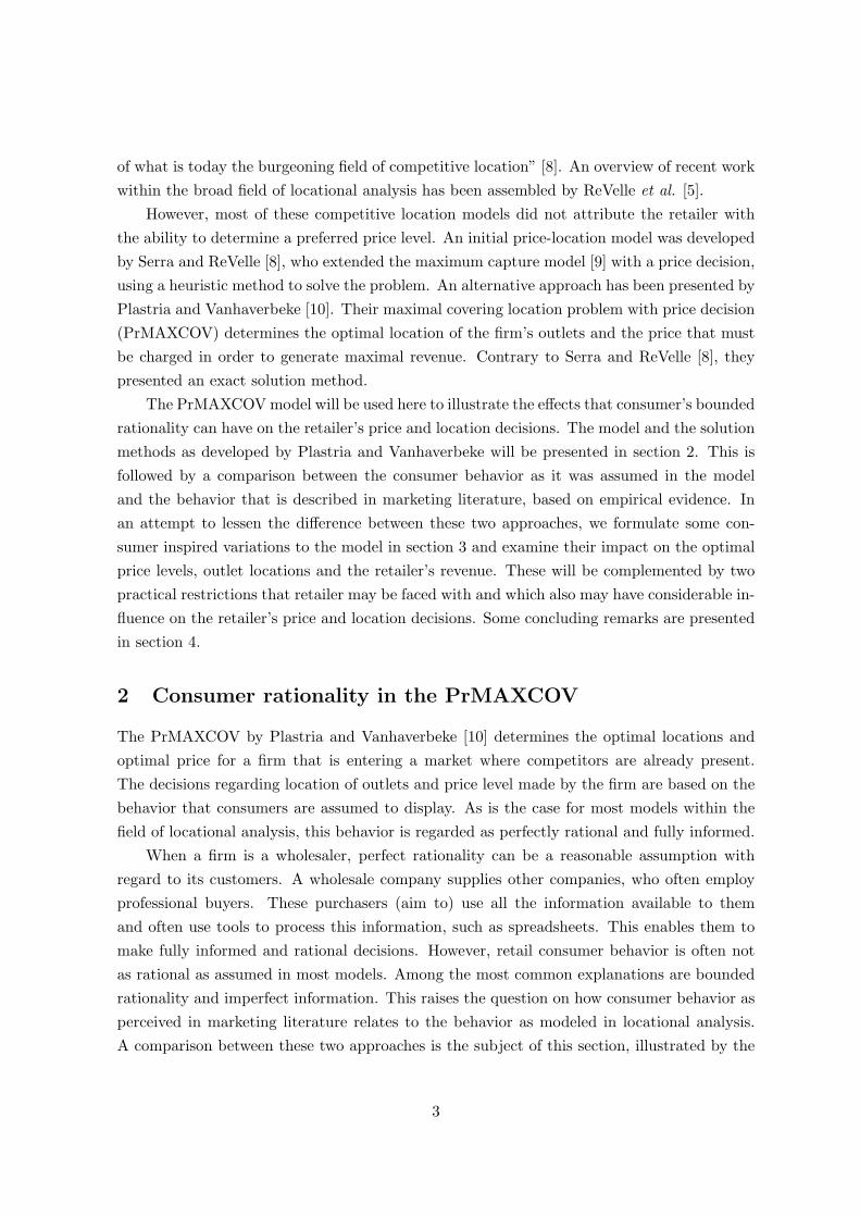
Figure 1 shows the separate steps of the decision making process as it is assumed in thePrMAXCOV. Firstly, customers will need to have access to a lot of information in order toevaluate all outlets in the market, as equation (2) includes many parameters. This meansthat in order to make a decision based on the criteria in equation (2), customers must acquireand have access to all of this information. This includes the transportation cost, the newfirm’s price, the distance to the new firm’s nearest outlets, the competitors prices, and thedistance to the competition’s outlets.

Figure 1: The consumer purchase decision in the PrMAXCOV.

When the consumer obtains all information, he will neatly compute the total costs facedwhen shopping at a given outlet. This means determining the cost to get there and adding themill price, charged at the outlet. Finally, the consumer decides at which outlet it is cheapestfor him/her to buy the product.

When modeling the behavior of firms, rationality and access to information are plausibleassumptions. When firms decide where they will locate their new outlets and which price tocharge, they aim to acquire as much relevant information as possible. This enables trainedpersonnel to process this information in order to make the best possible choices. In sucha decision making process, models such as the PrMAXCOV [10] can provide considerableassistance in determining the best options for the firm.

However, the firm that wants to enter a new market will evidently sell its products toany customer who has demand for the product. The question raised here is how this rational,informed behavior relates to consumer behavior as described in marketing literature? Itappears that when a firm is active in a business-to-customer or retail market, customers areoften far from rational. In what follows, several examples from marketing literature will be

8

provided where empirical findings indicate that consumer behavior differs significantly fromthe process that was described in figure 1.

Shugan states it like this: “consumer rationality is a property of the researcher ratherthan the consumer” [2]. Although his remark is directed towards marketing research, it alsoapplies to locational analysis. He predicts that “a clear and fundamental understanding ofconsumer behavior should help us more accurately predict consumer reactions to marketinginterventions”. Translating this statement to the models that were discussed above, thismeans that the goal must be to model consumer behavior as closely to reality as possible.This will in turn increase the predictive power of the models in terms of the customersreactions to the location and price decision of the firm.

In the following sections, we present some findings from marketing literature. Theseempirical results, illustrating the consumer’s bounded rationality, inspired the modificationsthat are discussed in section 3.

2.2.1 Information seeking and knowledge

The first step in the consumer decision making process in the PrMAXCOV consists of gath-ering the relevant information. To make the trade-off between the different outlets in themarket, the customer must acquire all prices, transportation costs and distances between hislocation and the outlets. Although consumers generally tend to be not that well informed,some variation may exist.

In an early attempt to distinguish the different types of consumer that may exist, interms of information seeking, Claxton et al. [16] developed a numerical taxonomy. Con-sidering only the purchase of durable goods, their taxonomic approach made it possible “toclassify buyers into distinctive groups in terms of their prepurchase search patterns”. Theyfound three measures (number of information sources used, total visits to stores, and de-liberation time) that allowed them to identify three general clusters of customers based onthe information seeking behavior. These were labeled “thorough (store intense), thorough(balanced) and non-thorough”, which were further subdivided into “subclusters varying indeliberation time” [16]. Their results provide clear evidence that consumers can be dividedinto segments based on information seeking behavior.

More recently, Schmidt and Spreng [17] suggest that many variables influence prepurchaseinformation search, but these effects are mediated by four variables: ability, motivation, costand benefit. They integrated a psychological framework concentrating on personal aspectsof the consumer with an economic framework that focuses on monetary costs and benefits.Based on these four variables, a consumer’s information search effort can be predicted andthus the information that will be used in the eventual purchase decision.

With the aim of finding a basis for pricing differentiation in the retail grocery market,Berne et al. [18] performed a cluster analysis to identify consumer profile based on their

9

price-information-seeking behavior. They found “two clearly separated clusters: high andlow intensity price-information seekers”[18]. This means that, based on their survey, a num-ber of customers will spend much time and possibly money in the search for price information,while others will be satisfied with the information that is readily available.

Following this initial article, Berne et al. [19] stated two years later that “there hasbeen an overestimation of the proportion of consumers who actively search for prices”. Theyempirically examined factors which may influence consumer information-seeking behavior.Their results showed that human ability holds “the greatest predictive power to explain thetendency for price comparison”. This confirms the findings of Schmidt and Spreng [17]. Ac-cording to the study, “overall market knowledge and previous investment in price search arethe principal predictors of price search”. Also analyzing demographic characteristics, Berne etal. found that “the higher the age of the consumer, the greater his/her tendency to compareprices”[19].

These findings indicate that it would be advisable to be able to distinguish different typesof customers, based on these characteristics. Yet, in the PrMAXCOV it was assumed that allcustomers react in the same way to the price and locations of the firm and that they use thesame amount of information.

A factor not considered by Berne et al. was the type of product. An alternative studyby Aalto-Setala and Raijas investigated “the degree of consumers’ price-consciousness, takinginto account the price dispersion of the grocery products that are at least physically homo-geneous” [20]. This relates more closely to the assumptions of the PrMAXCOV [10].

Based on empirical data containing the “price observations of eight grocery items in 82grocery stores in Finland” and the results of the interview of 1000 Finnish consumers byphone, Aalto-Setala and Raijas conclude that “the consumers were very well informed aboutthe price of homogeneous products such as milk and sugar” [20].

Although the study by Aalto-Setala and Raijas is limited to Finnish consumers and gro-cery products, it may be seen as supportive of the assumptions on consumer price knowledgein the PrMAXCOV. These, or any other, studies did not include consumer knowledge on thetransportation costs and the distance to outlets. One can never really claim to have searchedthe entire literature on consumer behavior, but so far we have not found any studies in thisparticular topic. Yet, this information was also required to make the fully informed purchas-ing decision that was assumed in the PrMAXCOV. This could be an interesting avenue forfurther research.

Concluding, when working under the assumption of a homogeneous product, consumershave relatively good price knowledge. We make abstraction of the consumer knowledge oftransportation costs. In the following sections, we will assume that consumers who are well in-formed on prices also have access to additional information to make an informed decision. Wewill now turn to the next part of the purchase decision, where this information is processed.

10

2.2.2 Information processing

Assuming that consumers have access to all the information they require, the question re-mains how much of this information they will use in their decision making process. Stivingand Winer state that “when consumers evaluate the price of a good, they may consider thewhole price, as assumed by most marketeers and economists, or they may use some heuristicto simplify the task” [21]. Plastria and Vanhaverbeke [10] clearly follow the former reason-ing, rather than the heuristic approach. The comparison between both approaches will bepresented here, followed by some computational results in section 3.1.

When looking at the results in the original article [10], the price ending digits were dividedmore or less equally between all digits from 0 to 9. However, this is not the case in manyretail outlets. The vast majority of price-endings are of the numbers 0, 5 or 9. Schindler andKirby [22] empirically found that, out of 1,415 advertised prices, 27.2% ended in 0; 18.5%ended in 5 and 30.7% had 9 as the rightmost digit. This means that those three digits madeup a vast majority of 76.4% price endings. Similar, older studies are provided by Gendall etal. [23].

The practice of setting prices just below the even level is most often referred to as “oddpricing” [21, 22, 23]. Strictly speaking, odd pricing can refer to any price that is not a roundprice, or “prices ending in one of the odd digits 1, 3, 5, 7 or 9” [24], but here it will refer to“a price set slightly below a round number” [25].

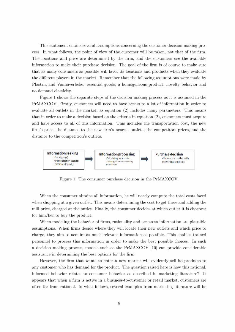
For a long time “the results of attempts to validate the assumption that odd prices leadto greater than expected demand have been mixed and inconclusive” [23]. Several theorieshave been developed over the years in order to explain the positive effect that odd pricingis believed to have on sales. These theories aim to provide a conclusive rationale for thedisproportional use of “just below prices” [25] in retail. Figure 2, developed by Stiving andWiner [21] shows the different explanations for price endings. One slight difference with theiroriginal schematic is our addition of the monetary unit to the operations category.

The two original explanations within the operations category, presented by Stiving andWiner [21], were not examined in great detail. One possible reason for charging prices justbelow the even level, given by Schindler and Kirby [22], is “because most customers paid ineven-dollar amounts, a 9-ending price would oblige clerks to use the cash register to makechange and thus reduce their opportunity to pocket the payment”.

We pose that monetary unit should be added as a third explanation within the opera-tions category. The price endings available to a firm are restricted to multiples of the smallestdenomination in circulation in the countries in which it is active. This is illustrated by thecase of Finland, where the one and two eurocent coins have been taken out of circulation,although they remain legal tender. This obliged retailers to make sure that the bottom lineon each bill is a multiple of five cents, as individual products may still have prices that aremultiples of one cent. Under our assumption of only one product, this implies that the price

11

would have to be a multiple of five cents.

Figure 2: Explanations for price endings based on [21], with the addition of the categorymonetary unit.

The image effects, featured in the right hand of figure 2, are also not relevant in thecontext of the PrMAXCOV. This group of theories assumes that the price, or the form ofthe price, projects a certain image of the product to the customer. Different explanationshaven been provided, e.g. that “odd prices indicate low-quality merchandise” [21]. A moredetailed analysis is provided by Schindler and Kibarian [26], who also found that a “99 priceending decreased the viewer’s perception of the quality of the advertised item, as well as of thegeneral merchandise quality and the retailer’s classiness”. Here, as we continue to work underthe assumption of homogeneous products, no differentation is made based of the quality ofthe product.

The most interesting price ending effects, from the viewpoint of the PrMAXCOV, are the“level effects” [21, 24, 25]. These level effects, “also known as underestimation effects, referto the behaviors or underlying processes that cause a consumer to distort their perception ofthe price” [21]. The underlying idea in these theories is that consumers do not include theprice he/she reads correctly in his/her memory, which is often referred to as the “drop-offmechanism” [27].

Several explanations have been presented in the literature: rounding down, comparingprices left to right and the limited memory capacity of the consumer. Stiving and Wineralready noted that “if consumers actually round down prices, firms would have a great in-centive to use just-below prices, providing a explanation for the observed price endings” [21].This means that retailers would be best off to maximize the rightmost digits of prices, asconsumers do not take them into account in their decision making process.

Bizer presented a study in which the goal was to “directly test whether consumers do in-

12

deed tend to drop off rightmost numerical digits” [27]. His experiment consisted of giving histest subjects a hypothetical budget ($73) and they were asked to estimate the number of itemsthat could be purchased with this budget. “The ending digits of the price was varied—halfof the time it was a 99-ending price (e.g., $2.99, $4.99) and the other half of the time it wasthe 00-ending price one penny higher (e.g., $3.00, $5.00)” [27]. He found that “respondentsestimated that significantly more items with 99-ending prices could be purchased for a givenamount of money than items with the 00-ending prices only one cent higher”, which provides“direct evidence for the existence of the drop-off mechanism in price information processing”.Other empirical studies were performed by Manning and Sprott [25] and Gueguen et al. [28],who largely confirm Bizer’s results in different settings.

When considering the rationale of the drop-off mechanism, it can be said that the PrMAX-COV underestimates the revenue that a firm may generate when entering a market. The modelassumes that the consumer considers the whole price when he/she makes his/her purchasingdecision. The analysis made in marketing literature, discussed above, indicates the opposite.Consumers generally compare price from left to right, even ignoring the right most digitsentirely.

Assuming that consumers indeed ignore the right hand digits (usually the decimals), re-tailers should implement this form of irrational behavior in their location decision. For thePrMAXCOV, this would imply determining the demand covered based on rounded prices, andsubsequently maximizing the decimals (to .99) as customers do not include them in the de-cision making process. In section 3.1, some computational results will be presented, showingthe impact of the drop-off mechanism on the firm’s revenue.

3 A consumer based approach to the PrMAXCOV

From the previous section, it may be clear that there exist considerable discrepancies betweenconsumer behavior as it is assumed in marketing literature and in location analysis models.We will now present three modifications to the original model, addressing some of theseconcerns. Together with implementing a more consumer oriented approach, we provide ananswer to a question raised by Plastria and Vanhaverbeke:

“The price setting in a retail outlet does not allow for the very precise figureswe propose here. We are interested to see the impact of rounded prices on thesolution of the model. Another option we consider is the use of a selective pricechoice heuristic. Imagine the retailer to be interested in certain ranges of price,what would be the effect on the optimal model solution?” [10]

This question can be divided into two separate issues: the impact of rounded prices andthe effect of price ranges on the solution of the model. The first issue regarding rounded

13

pricing will be examined in section 3.1, which in turn allows the implementation of the drop-off mechanism. The impact of price ranges on the solution of the problem is subsequentlypresented in section 3.2. Finally, in section 3.3 an alteration to the definition of the coveringsets is discussed, allowing for the differentiation between different consumer types.

The results presented below were generated using the procedure and model that wasdeveloped by Plastria and Vanhaverbeke. They wrote the program in AMPL (A ModelingLanguage for Mathematical Programming, Version 20021038) and solved using ILOG CPLEX9.1. One slight difference is that for this paper version 20080925 was used for AMPL andversion 11.0 for CPLEX to calculate the results. The hardware used is the same as in theoriginal article, namely a Intel Xeon CPU 3.4GHz, with 2GB RAM, running Windows XPProfessionel SP2. To allow for comparison of the results, we used for the most part the samedata that was used in the original article. Throughout what follows, the results for the smallcase and the large case [10] are presented to allow for a smooth comparison with the originalresults. The test data are available at http://homepages.vub.ac.be/vlvhaverb/testdata.html.

As described in [10], the small case considers the region of the Belgian capital (Brussels).There are 33 customers (I), 6 existing competitors (C) whose price varies randomly between55 and 67 and there are 10 locations at which the firm can potentially locate (J). Thedistances were calculated on the road network and the demand was randomly generated withvalues between 20 and 39. The large case was completely artificially generated, with 1,000customers whose x- and y-coordinates are random between 0 and 100 as well as their demandthat lies between 20 and 50. There are 100 potential locations for the new firm to open anoutlet with 20 competitors already present in the market. In the large case, the distances areEuclidean.

3.1 Rounded pricing and drop-off mechanism

From the computational results presented in [10], it might appear that there is no problemwith the number of decimals from a practical point of view. The tables containing the resultsfor the three datasets only show two decimals for the optimal prices. However, these are notthe exact optimal solutions to the problem. In reality, the exact prices often had up to ninedecimals.

It may be clear that when dealing with the exact solution of the model, there arisesa problem in terms of practicality. When a firm decides to implement the optimal pricingpolicy that the model calculated, an obvious restriction exists on the number of decimals.All prices are bound to the currency of the country in which the firm wishes to locate itself.For most currencies the smallest denomination is one cent, representing one hundredth of thebase value. This means that in practice prices are limited to two decimals, as all prices mustbe multiples of the smallest denomination in circulation. In this respect, Finland is an evenmore restrictive case, in that all prices must be multiples of five cents.

14

Intuitively, calculating the exact optimal solution and rounding the optimal price to thenearest feasible value appears to be the simplest approach in dealing with this issue. This isalso the method used by Plastria and Vanhaverbeke. An alternative approach will be proposedhere, namely ensuring in advance that the solution calculated by the model is rounded andthus practically feasible.

Ensuring that the solution of the model is a rounded value can be done by an alteration inthe first step of the solution procedure of the model. Depending on the smallest denomination,available for a given problem, the list P is replaced by an artificial list Pa, consisting ofmultiples of this smallest denomination (a). It is also manually ensured that the list Pa

consists solely of unique prices, making properties 8 and 9 from the PrMAXCOV redundant.As the list Pa is artificial, independent of the problem under consideration, the question

arises how long the list will have be, in order to ensure a maximal solution. The answer is asfollows: the maximal price pa ∈ Pa must be the highest multiple of the smallest denomination(a) which is still less or equal to the maximal critical price (maxP ). This can be explained bythe fact that any price larger than the maxP will not undercut the existing minimum totalprice pij for any customer i at any new outlet j, so no customer will patronize any outletsituated at any location j ∈ J . In other words, no demand will be covered, so this can neverbe an optimal solution to the problem. This means that the list Pa will be finite and willcomprise of maxP/a prices.

In the presentation of the model in section 2.1 it was mentioned that two solution methodswere developed for the PrMAXCOV, a full enumeration method and a faster, intelligentmethod. As the latter is based on the properties of the list P , it cannot be used when workingwith Pa. Although the fifth property developed by Plastria and Vanhaverbeke remains valid,the final four properties do not. They rely on the relation between the covering sets for twoconsecutive critical prices pij ∈ P , which does not exist when working with the artificial pricespa.

Now we can turn to the question how the solution of the unrestricted model ( Π∗) willrelate to the solution using the artificial, rounded prices ( Π∗a). Generally, it can be expectedthat adding restrictions to a model will decrease, rather than increase, the optimal value ofany problem. Plastria and Vanhaverbeke noted that they “only need to examine prices in P ,i.e. of critical price type pij” [10], meaning that only these prices can result in an unrestrictedoptimal solution. This implies that no price pa ∈ Pa will result in higher revenue for the firm.

The interesting question is whether or not the optimal price determined using the listPa will be the same as rounding the unrestricted optimal price to the nearest multiple of thesmallest denomination (a). Table 1 makes this comparison with respect to the large case usedby Plastria and Vanhaverbeke.

Table 1 shows the optimal price and revenue for both the unrestricted calculation as wellas for the model using the rounded pricelist Pa. It may be clear that the unrestricted solutions

15

Budget Optimal price Optimal revenueB p∗ p∗0.01 p∗0.05 p∗1

∏∗ ∏∗0.01

∏∗0.05

∏∗1

1 10.8194 10.81 10.35 10 21,153.69 21,135.21 21,121.37 20,899.842 103572 10.35 10.35 10 38,187.32 38,160.80 38,160.80 37,576.383 4.9742 4.97 5.00 5 54,888.86 54,842.64 54,638.28 54,638.284 5.0279 4.97 5.00 5 71,416.11 71,348.48 71,243.74 71,243.745 5.0577 5.05 5.05 5 84,369.53 84,240.41 84,240.41 84,122.666 5.0279 5.02 5.00 5 96,049.78 95,898.15 95,740.54 95,740.547 5.0577 5.05 5.05 5 106,814.30 106,650.84 106,650.84 106,378.108 5.0577 5.03 5.05 5 116,318.73 116,153.98 116,140.72 115,685.669 5.0577 5.05 5.05 5 123,975.42 123,785.69 123,785.69 123,254.9410 5.0554 5.05 5.05 5 129,698.72 129,560.53 129,560.53 128,895.02

Table 1: Comparison between the optimal price and revenue for the unrestricted model andthe restricted solution for three values of a. Several values of the variable B are presented.

p∗ and Π∗ are the results that were already determined by Plastria and Vanhaverbeke [10].Note that the columns p∗0.05 and Π∗0.05 are an illustration of the case of Finland, with thesmallest denomination being five eurocent.

It appears that there exists a negative relation between amount of the smallest denomina-tion and revenue. Obviously, when the solution for a certain value of a (e.g. 0.01) is possiblefor a larger value of a (e.g. 0.05), the revenue will be the same. When this is not the case, anincreased value of a will, ceteris paribus, result in a reduced revenue as the set Pa from whichthe solution can be drawn becomes smaller. We know for certain that p∗0.05 ∈ P0.01, while onthe other hand it is only by coincidence that p∗0.01 ∈ P0.05 may occur.

Looking at the price, in most cases the pa is the closest rounded value of the unrestrictedoptimal price p∗. One exception is the case of B = 1, where it would be expected thatp∗0.05=10.80, but calculations showed that p∗0.05=10.35. This implies that, instead of using theunrestricted model and rounding the optimal solution, it would be advantageous for a firmto use the restricted model.

Of course, the PrMAXCOV not only determines the optimal price p, but also the optimallocations at which the firm must open (an) outlet(s). However, from our analysis it appearsthat these optimal locations are not influenced by the use of rounded pricing. This does notexclude the possibility that some minor differences in the set of optimal location are possible.These may exist when, due to the rounding, the critical price of an important demand pointis crossed resulting in a significant loss in demand. In the datasets presented here, no suchinstances appeared. Important to note is the fact that the relative importance of demandpoints depends to some extent on the level of aggregation. For a more detailed discussion onthis subject see [12].

The drop-off mechanism that was presented above states that consumers generally do

16

not take into account the whole price of a product when making a purchase decision. Sev-eral explanations have been examined in literature, such as bounded memory capacity orleft-to-right comparison. Applying this logic to the PrMAXCOV model by Plastria and Van-haverbeke [10], it implies that the demand by consumers is in fact based on the whole partof the price and that they make abstraction of the decimals. This in turn means that thedemand calculated by the model is an underestimation of the demand that will actually becovered.

Table 2 gives an indication of the impact on the solution of the PrMAXCOV, if the level-effect is considered. It shows that the revenue increases when the rationale of the drop-offmechanism is used. The p∗, D∗ and Π∗ are the respective optimal price, demand and revenuethat were generated using the original PrMAXCOV.

Budget Optimal price Covered demand Optimal RevenueB p∗ p∗c p∗r D∗ D∗c

∏∗ ∏∗c

∏∗l

1 10.8194 10 10.99 1,955.16 2,089.98 21,153.69 20,899.84 22,968.922 10.3572 10 10.99 3,687.03 3,757.64 38,187.32 37,576.36 41,296.443 4.9742 4 4.99 11,034.71 11,836.48 54,888.86 47,345.94 59,064.044 5.0279 5 5.99 14,203.96 14,248.75 71,416.11 71,243.74 85,350.005 5.0577 5 5.99 16,681.40 16,824.53 84,369.53 84,122.66 100,778.956 5.0279 5 5.99 19,103.36 19,148.11 96,049.78 95,740.54 114,697.177 5.0577 5 5.99 21,119.15 21,275.62 106,814.30 106,378.10 127,440.968 5.0577 5 5.99 22,998.35 23,137.13 116,318.73 115,685.66 138,591.429 5.0577 5 5.99 24,512.21 24,650.99 123,975.42 123,254.94 147,659.4210 5.0554 5 5.99 25,655.48 25,779.00 129,698.72 128,895.02 154,416.23

Table 2: Comparison between revenue generated by the PrMAXCOV and the revenue gener-ated using the level-effect, for the large case.

The difference between the original revenue (Π∗ = D∗.p∗) and the revenue incorporatingthe level-effect (Π∗l = D∗c .p

∗r) can be attributed to two separate influences. On the one hand

the price perceived by the consumers (p∗c) is lower than the optimal price (p∗). This wasdetermined using the method described above. This lower price leads to consumer demand(D∗c ) that is higher or equal to the demand covered in the optimal solution (D∗), followingthe third property of the full enumeration method [10]. Multiplying this rounded price andthe associated demand it generates, gives the revenue based on rounded prices (Π∗c = D∗c .p

∗c)

which was discussed above and was shown to be lower or equal to the unrestricted optimalsolution.

However, from the literature on the drop-off mechanism, it appears the consumers wouldnot take into account the left most digits in prices when making their purchase decision. Thisprovides an incentive for the retailer to maximize the digits that consumers do not notice (or

17

remember), as it will not affect the demand covered. In this case it means that the retailerwill charge a price that is just below the next whole value (p∗r). The revenue incorporationof the level-effect (Π∗l ) thus equals the price charged by the retailer (p∗r) multiplied with thedemand (D∗c ), based on the price that the consumers perceive (p∗c).

Noteworthy is the fact that the price that consumers perceive will not always be therounded price as we defined it here. Consumers tend to make abstraction on the right mostdigits in the price, not just the decimals. If the product under consideration would be a fairlyexpensive product costing thousands or hundreds, it could be that even unit digits would beleft out of the decision, as they then represent a relatively small part of the monetary cost.And the retailer would therefore have an incentive to maximize these unit digits. There havenot been any studies examining this specific relation between price level and the measure ofthe drop-off, so we will assume here that only the decimals are not taken into account.

These results indicate that a firm could benefit from examining the specific (irrational)consumer behavior that its customers show. Understanding the way in which the firm’scustomers process the price information could result in higher revenue for the firm or at leasta better anticipation of the revenue that may be generated by charging a certain price.

3.2 Price ranges

In this section, we will turn to the second issue raised by Plastria and Vanhaverbeke [10] intheir concluding remarks: “what would be the effect of price ranges on the solution of themodel?” In this remark, they mention the possibility of the retailer, i.e. the firm, to beinterested in certain ranges of price. Alternatively, a price range could be imposed by somegoverning agency.

The goal here will be to assess the impact that such price ranges may have on the revenueof firms. In the above sections, there was only one bound on the price, formulated in equation(10). A minimum price is defined, to assure that firms do not sell below cost. Up until nowthis pmin was held constant at 0. Implementing price regulations can be achieved quite easilyin the model, by using equation (17) instead of equation (10):

pmax ≥ p ≥ pmin (17)

Implementing price ranges in the model requires only a minor alteration in the firststep of the algorithm. Instead of considering all critical prices in the list P , only the pricesthat fall within the permitted range will be considered. The sole consequence for the modelwill therefore be that the list P will become shorter. As no further changes are needed, allproperties described by Plastria and Vanhaverbeke [10] remain valid. Note that in this sectionthe original algorithm is used, and not the method proposed in the previous section usingrounded prices. This is done to clearly show the isolated impact of the price regulations in

18

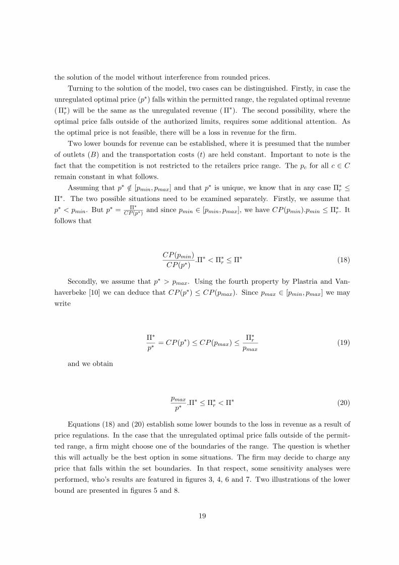
the solution of the model without interference from rounded prices.Turning to the solution of the model, two cases can be distinguished. Firstly, in case the

unregulated optimal price (p∗) falls within the permitted range, the regulated optimal revenue( Π∗r) will be the same as the unregulated revenue ( Π∗). The second possibility, where theoptimal price falls outside of the authorized limits, requires some additional attention. Asthe optimal price is not feasible, there will be a loss in revenue for the firm.

Two lower bounds for revenue can be established, where it is presumed that the numberof outlets (B) and the transportation costs (t) are held constant. Important to note is thefact that the competition is not restricted to the retailers price range. The pc for all c ∈ C

remain constant in what follows.Assuming that p∗ /∈ [pmin, pmax] and that p∗ is unique, we know that in any case Π∗r ≤

Π∗. The two possible situations need to be examined separately. Firstly, we assume thatp∗ < pmin. But p∗ = Π∗

CP (p∗) and since pmin ∈ [pmin, pmax], we have CP (pmin).pmin ≤ Π∗r . Itfollows that

CP (pmin)CP (p∗)

.Π∗ < Π∗r ≤ Π∗ (18)

Secondly, we assume that p∗ > pmax. Using the fourth property by Plastria and Van-haverbeke [10] we can deduce that CP (p∗) ≤ CP (pmax). Since pmax ∈ [pmin, pmax] we maywrite

Π∗

p∗= CP (p∗) ≤ CP (pmax) ≤ Π∗r

pmax(19)

and we obtain

pmax

p∗.Π∗ ≤ Π∗r < Π∗ (20)

Equations (18) and (20) establish some lower bounds to the loss in revenue as a result ofprice regulations. In the case that the unregulated optimal price falls outside of the permit-ted range, a firm might choose one of the boundaries of the range. The question is whetherthis will actually be the best option in some situations. The firm may decide to charge anyprice that falls within the set boundaries. In that respect, some sensitivity analyses wereperformed, who’s results are featured in figures 3, 4, 6 and 7. Two illustrations of the lowerbound are presented in figures 5 and 8.

19

All of the following results are based on the small case. The transportation costs wereheld constant at t = 0.01. Other sensitivity analyses were performed using different values for(t), but the conclusions were the same. The numbers of outlets (B) that were opened variedfrom 1 to 5.

Figure 3 shows the relation between the value for the upper bound of the price regulation(pmax), and the optimal price (p∗r) that was determined by the model under the given regu-lation. The pmax varied between 56 down to 30 with increments of 2. The reader may noticethat the scale on the horizontal, showing pmax, is inverted. This to illustrate the relationbetween the optimal price solution and the restrictiveness of the upper bound on the price.

Figure 3: Sensitivity of the optimal price p∗r to varying pmax.

The left most part of the chart shows the unrestricted optimal prices. Without imposinga pmax, the highest p∗ is 52.41 (B=5). Imposing a pmax of 56 will not have any impact inthe solution of the model. The chart clearly shows that when the imposed range becomesrestrictive (p∗ > pmax), firms will charge prices that are equal to or slightly less than thepmax. In this particular example, it appears that it is advantageous for the firm to chargeless than what is allowed, which indicates that the difference in price is compensated by anincrease in demand. However, restricted prices are relatively close to the upper bound. Thisshows that low prices will not result in sufficient increases in demand, although these mighttheoretically generate higher revenues. Whether or not the restricted prices remain equal tothe pmax or fall slightly below depends to a large extent on the location of the demand pointsin the problem under consideration.

The impact on the firm’s revenue is shown in figure 4. We know from figure 3 that in

20

most cases p∗r is relatively close to pmax. Theoretically, a reduction in price could result in anincrease of the covered demand, leaving revenue relatively unaltered. However, figure 4 showsthat this is not the case in the example presented here. The firms are faced with decliningrevenue as the price regulation becomes more severe, meaning that pmax becomes smaller.Again here the scale on the horizontal axis is inverted, to illustrate the loss in revenue inrelation to the restrictiveness of the price range.

The curve for the case of B=1 remains unchanged for most values of pmax. This is becausethe optimal solution without a price range is 33.21. So the optimal revenue is only affectedwhen pmax is lower than this threshold.

Figure 4: Sensitivity analysis of the optimal revenue Π∗r to varying pmax.

With an increasing severity of the price restriction, it can occur that some outlets nolonger generate additional revenue and thus become redundant. This can be seen in figure 4when, at certain values of pmax, the curves for different values of B start to coincide. Begin-ning at pmax = 40, the revenue generated by four and five outlets is the same. This meansthat the fifth outlet does not contribute to the retailer’s revenue. Even more striking is thefact that a fourth and fifth outlet are useless when pmax ≤ 34. Under this very restrictiverange, a firm can only open three demand covering outlets.

This remarkable effect can be explained by the fact that the prices charged by the com-petition are not subject to the restriction of the maximum price. Given the relatively lowprice charged by the new firm in the market, imposed by the restriction, most demand pointswill choose the entrant. The demand points that continue to prefer the competition will bethose that are situated very close to them, benefiting from low transportation costs. In order

21

to compensate for higher transportation costs, the new firm would have to charge an evenlower price. Given the restriction of uniform pricing, this would mean a decrease in revenue.Therefore, it is beneficial for the firm to ignore the demand points that are located very closeto the competition and charge a higher price, rather than try to cover the entire market. Aninteresting avenue for further research could be to consider volatile prices by the competition.

Figure 5 illustrates how the optimal solution with price ranges compares to the lowerbound that was established in equation (20). Obviously, the maximal revenue for the prob-lem without the price ranges will always be larger or equal to the maximal revenue underprice ranges. The lower bound on the revenue is only shown for the range in which theimposed maximum price is restrictive, when p∗ > pmax. Outside of this range the imposedprice is non-restrictive, thus making lower bound without meaning because the unrestrictedoptimal revenue (Π∗) is feasible. The reader may notice that the maximal revenue with priceranges is the same as the curve for B=5 in figure 5. In this example, the revenue for a givenmaximum price is always higher than the calculated lower bound. The narrower the range(lower maximum price), the lower the maximal revenue will become for a given problem. Thisindicates that the reduction in price is not compensated by an increase in covered demandfor this example. Other examined instances showed very similar evolutions.

Figure 5: Illustration of the lower bound for B=5 for different values of pmax.

Until now, only the case of a maximal limit on the price was considered. Therefore, asensitivity analysis was made on the variable pmin. The results of this analysis are summarizedin figures 6 and 7.

Depicting the relation between the variable pmin and the restricted optimal price (p∗r),figure 6 shows that p∗r reacts slightly differently when the price range is narrowed from below.

22

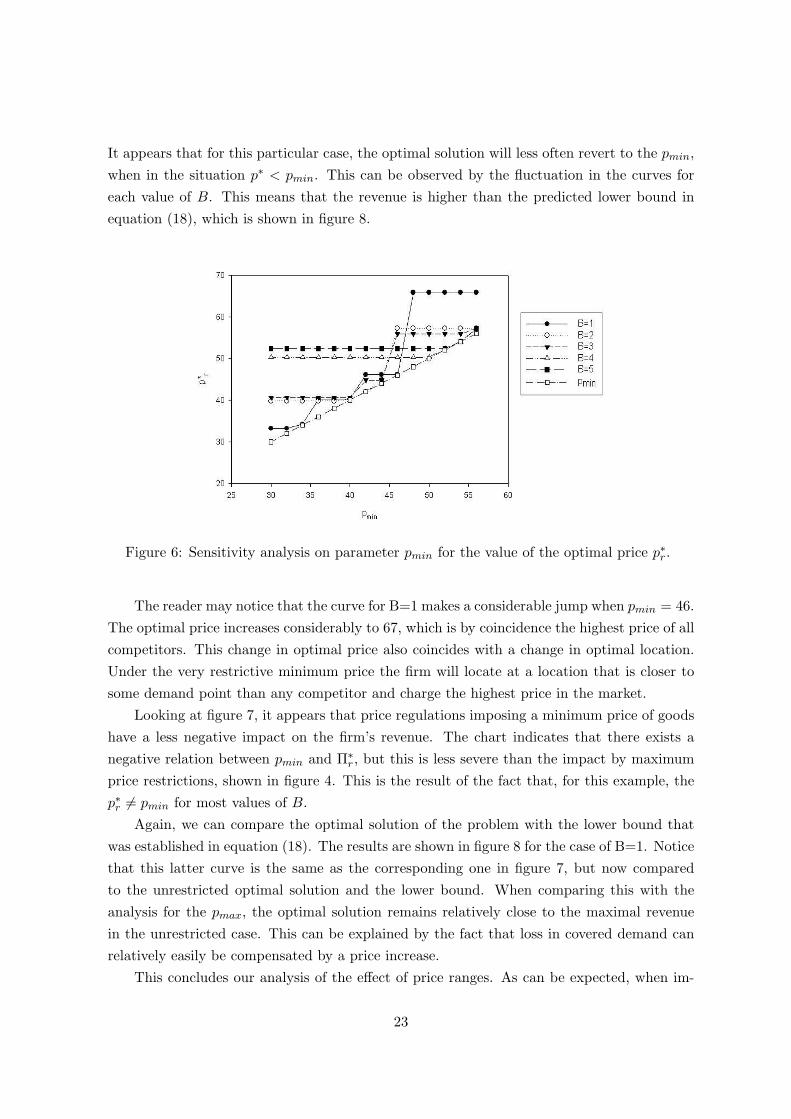
It appears that for this particular case, the optimal solution will less often revert to the pmin,when in the situation p∗ < pmin. This can be observed by the fluctuation in the curves foreach value of B. This means that the revenue is higher than the predicted lower bound inequation (18), which is shown in figure 8.

Figure 6: Sensitivity analysis on parameter pmin for the value of the optimal price p∗r .

The reader may notice that the curve for B=1 makes a considerable jump when pmin = 46.The optimal price increases considerably to 67, which is by coincidence the highest price of allcompetitors. This change in optimal price also coincides with a change in optimal location.Under the very restrictive minimum price the firm will locate at a location that is closer tosome demand point than any competitor and charge the highest price in the market.

Looking at figure 7, it appears that price regulations imposing a minimum price of goodshave a less negative impact on the firm’s revenue. The chart indicates that there exists anegative relation between pmin and Π∗r , but this is less severe than the impact by maximumprice restrictions, shown in figure 4. This is the result of the fact that, for this example, thep∗r 6= pmin for most values of B.

Again, we can compare the optimal solution of the problem with the lower bound thatwas established in equation (18). The results are shown in figure 8 for the case of B=1. Noticethat this latter curve is the same as the corresponding one in figure 7, but now comparedto the unrestricted optimal solution and the lower bound. When comparing this with theanalysis for the pmax, the optimal solution remains relatively close to the maximal revenuein the unrestricted case. This can be explained by the fact that loss in covered demand canrelatively easily be compensated by a price increase.

This concludes our analysis of the effect of price ranges. As can be expected, when im-

23

Figure 7: Sensitivity analysis on the value of the optimal revenue Π∗r for different values ofthe pmin.

Figure 8: Illustration of the lower bound for B=1 for different values of pmin.

posing additional restrictions on the solution of the problem, there will be a loss in optimality.It appears from the analyses presented here that imposing a minimum price on product willhave less severe effects of the firm’s revenue than a maximum price.

24

3.3 Consumer segmentation

Up to this point, we have implicitly assumed that all consumers make their purchase decisionin the same manner, using the same information in the process. However, we know fromsection 2.2.1 that this is generally not the case in the retail market. For example, Berne etal. [18] made the distinctions between high and low intensity price-information seekers. Thismeans that some customers will go to great length to acquire price information, while othersmake little or no effort to get and use price information in their purchase decision. Therefore,this section is devoted to the differentiation between these consumer types.

In the PrMAXCOV, the consumer’s purchase decision process is described by the patron-izing set Ni(p), for every consumer i. A consumer will be covered by the new firm when itopens a new outlet j ∈ Ni(p), while charging the price p. The patronizing set contains allfacilities for which the critical price is at least the p that is being considered. The respectiveformulas for the patronizing sets and critical prices are given in equations (3) and (4). Thesecan be determined for every demand point/customer i and every price p ∈ P .

To facilitate the consumer segmentation, we will attribute to each demand point i a con-sumer type zi. In what follows we will assume that zi ∈ {1, 2, 3}, meaning that we assumethe existence of three consumer types. If zi = 1, then the patronizing set is defined, as in theoriginal model, according to equation (4). These customer are fully informed and perfectlyrational, and have the capacity and time to compare every possible outlet in terms of priceand distance. Also, they are assumed to show novelty behavior.

The second customer type, if zi = 2, is similar to type 1 with the exception that theypresent conservative behavior, rather than novelty behavior. As described by Plastria [14],these conservative customers will go on “patronizing the existing facility they patronized be-fore” in case of a tie with the new facility. As mentioned in section 2, a tie can occur when,by accident, a customer’s total purchasing cost is equal for the existing and the new player.These customer’s patronizing sets are defined as follows:

Ni(p) = {j ∈ J : pij > p} ∀i ∈ I (21)

In the framework of Berne et al. [18] these two customer types could be designated ashigh intensity price-information seekers. Where the two previous consumer types are quitesimilar, type 3 customers will determine their preferred outlet differently. The consumerswith zi = 3 can be considered as a non-informed or non-rational type. In the discussion ofBerne et al. [18] they can be considered as the extreme case of low intensity price-informationseekers. These are the customers that will simply shop at the outlet that is located closest totheir location/home. This can be for a number of reasons. Perhaps the cost of the productis negligible compared to their total spending. They could also face restrictions in terms oftransport modes available to them. Alternatively, they do not have access to price information

25

or do have access, but not the time for intensive market research. A new firm’s outlet willcover the demand point if it is located closer than any of the competition’s existing locations.This is described in the following manner:

Ni(p) = {j ∈ J : dij ≤ minc∈C

(dic)} ∀i ∈ I (22)

Many more types could be distinguished, based on any number of factors, such as ageor profession. The three types described here only serve as an illustration of the concept ofdifferentiation. For example, a maximal distance could be imposed for the customers of type3, indicating that they will only consider the existing competition that is located nearby.

One important disadvantage to customer type differentiation in the PrMAXCOV is thefact that due to the alternative definitions for the patronizing sets, all properties defined byPlastria and Vanhaverbeke [10] become invalid. We can no longer rely on the relation betweenthe critical prices and the covering sets, as the covering sets for demand points with zi = 3become independent of the price that is being charged. This implies that it is no longerguaranteed that the optimal price must be a critical price. Indeed, it might happen that nooptimal price exists (see Plastria and Carrizosa [29]). Therefore, we shall use the roundedpricing method that was described above.

We will also use price ranges, as discussed in section 3.2, to avoid undesirable solutionsto the problem. Without imposing an upper bound on the solution of the model, the optimalsolution will always be an extremely high price. This is the result of the fact that the type3 customers do not include the price in their purchasing decision. Without any limitation,the new entrant in the market will simply locate at the locations that are closer to type 3demand points than any existing competing outlet and charge an exuberant price. This isnot a desirable result, as even a lazy or indifferent customer will eventually react to extremelyhigh prices. Therefore, we impose a maximum price on the solution of the model that is equalto twice the price of the most expensive competitor.

As we are obliged to use the full enumeration method the small case is used to illustratethe effect that consumer differentiation will have on the optimal solution of the problem.As there are 33 customers/demand points in the market, each consumer type is randomlyattributed to one third of the customers, resulting in 11 customers for each type. As themaximal pc = 65, we set pmax = 130 to avoid extreme solutions. To generate these solutions,we used the rounded pricing method that was described in section 3.1, with a = 0.01. Thetransportation costs were held constant at t = 0.01.

Looking at the results in table 3, it appears that the consumer differentiation has thelargest impact when only one outlet is opened (B=1). In that case, the optimal price withconsumer differentiation is nearly double the solution where all consumers are assumed tobe of type 1. In the other cases, prices are slightly higher or the same as in the originalmodel. What is striking is the fact that there is a loss in revenue in all instances. This can

26

Budget Without differentiation With differentiationB p∗

∏∗ p∗∏∗ ∏

UD

1 33.21 20,457.36 59.55 15,959.40 13,117.952 39.79 30,001.66 39.79 27,216.36 14,722.303 40.65 32,235.45 43.61 30,657.83 14,755.954 50.26 33,925.50 55.90 33,428.20 13,469.685 52.41 36,739.41 55.27 36,201.85 14,045.88

Table 3: Comparison between the optimal solution with and without consumer differentiation.

be explained by the fact that some consumers of type 3 will automatically be attributed tothe competition, which causes a decline in covered demand.

Looking at the graphical representation of the small case in figure 9 we can in part ex-plain the increase in price when consumers are differentiated. For the case of B=1 the optimallocation is site number 112, which can be seen at the center of the map. This is a centrally lo-cated outlet, relatively far from the competition and with many demand points in the vicinity.Remember that without differentiation all the demand points are of type 1. Therefore, giventhe optimal price the firm will reach a sizable portion of the total demand in the market.

However, with consumer differentiation the situation becomes very different. The optimallocation will now move to site number 100, which is located at the north-west border of themarket where some type 3 customers are located.

The effect of consumer differentiation is the clearest with B=1, but similar changes takeplace for other values of B. In general, the firm will rather locate close to the lazy or unin-formed customers to whom it can charge relatively high prices. However, the demand thatthe firm gains with these customers, is lost for type 1 and 2 customers because of the higherprice it will charge. Apparently in the example case presented here, the decrease in covereddemand is not compensated by the increase in price, resulting in the loss of revenue that isillustrated in table 3.

In the right most column of table 3 the revenue (ΠUD) is calculated that would begenerated by the firm when it uses the locations and price level that was calculated with-out consumer differentiation, in a market where consumer of all 3 types are present. In allinstances the ΠUD is considerably lower than the maximal revenue with and without differ-entiation. This clearly illustrates the importance of consumer behavior knowledge for a newentrant in a competitive market. If the firm would predict demand and revenue based onthe assumption that all consumer are perfectly rational and fully informed, while in fact aportion of the customers are subject to bounded rationality, then its actual results will bemuch lower than what the model would predict.

This exemplary case only serves as an illustration of the importance for a firm to un-

27

Figure 9: Graphical representation of the small case on a map of Brussels.

derstand its customers. If a firm were to decide to enter a new competitive market underthe assumption that all customers are fully informed and perfectly rational when this is inreality not the case, then the consequences on its results could be dramatic. As firms oftenuse locational analysis models as a decision making tool, it becomes important that thesemodels also include the differences in individual consumer decision making.

4 Conclusions and extensions

In most models within the field of operational research it is assumed that consumers areperfectly rational and fully informed. This is also the case for the maximal covering locationproblem with price decision developed by Plastria and Vanhaverbeke [10]. This rational be-havior, however, is not what is being found by studies stemming from marketing research.Several studies indicate that most retail consumers do not have access to all the informationrequired to make a fully informed purchasing decision. And in the event that they have theinformation it may still be that some consumers will not use it. In economics literature it isoften called bounded rationality. If a firm opens outlets at locations determined by modelsassuming perfectly rational customers it could be that the actual coverage, and thus revenue,generated by the firms will be significantly different from that what was calculated by themodel.

28

We started by comparing the consumer behavior as it was modeled in the PrMAXCOVwith the behavior that appeared from marketing surveys on price knowledge and purchasingdecision making. There appeared a considerable discrepancy between both approaches. Un-like what was assumed in the PrMAXCOV, a large portion of consumers does not make fullyinformed, rational decision. Often, they do not even have a good notion of the price that isbeing charged, let alone how this price compares to the competition.

With the aim of enhancing its applicability to real situations, we made three modifica-tions to the original PrMAXCOV model. This served the dual goal of answering a questionraised in the concluding remarks of the original paper as well as allowing an approach that ismodeled more closely to consumer behavior as observed in real life.

With the first modification, we investigated the impact of working with rounded pricesinstead of the very precise solutions that were calculated by the original model. Adding thisrestriction of the model reduced the optimality of the solution, as can be expected. However,it appeared that the rounded solution can in some cases be different from the rounded valueof the unrestricted optimal solution. Using the rounded prices allowed us to take the drop-offmechanism into account, where prices can be augmented to just below the next whole price,without loss of demand.

Secondly, the impact of price ranges was presented. In line with expectations, the rev-enue that could maximally be generated by the firm reduced drastically when limitations wereplaced on the prices that can be charged. A lower bound to the solution was determined andin the exemplary case considered here, the solution was consequently higher than this lowerbound. The negative effect on the revenue, as a result of imposed price restrictions, is shownto be greater when an upper bound is imposed, compared with an obligated minimum price.

Finally, the model was adapted in order to allow for differentiation between several typesof customers. For each type of customer a different decision rule was defined. This reflectsthe fact that in reality many consumers do not really take the price into account when mak-ing a purchase decision. Often they simply go to the store that is located nearest to them.The results showed that when customers with bounded rationality are present in the market,new firms will rather locate close to these demand points and charge relatively high prices,exploiting their indifference with regard to the price level.

One serious drawback of our approach is the fact that these modifications to the originalmodel excluded the use of the intelligent enumeration method that was developed by Plas-tria and Vanhaverbeke [10]. Given the necessity of using the full enumeration method onlysmaller case were presented to illustrate the impact of our modification on the optimality ofthe problem’s solution. The development of new properties, taking into account the consumerbased approach, would be an interesting avenue for further research.

29

References

[1] Vanhaverbeke L. Competitive location models and consumer spatial behaviour: Opti-mization models and an agent based approach; PhD dissertation, VUBPress, Brussels,2010.

[2] Shugan S. Are consumers rational? Experimental evidence?. Marketing Science 2006;25(1): 1-7.

[3] Simon H. Models of bounded rationality, The MIT Press, Cambridge, MA., 1982.

[4] Drezner T, Eiselt H. Consumers in competitive location models, in: Drezner Z, HamacherH (Eds.), Facility location: Application and theory, Springer, Berlin Heidelberg, pp. 151-178.

[5] ReVelle C, Eiselt H, Daskin M. A bibliography for some fundamental problem categoriesin discrete location science. European Journal of Operational Research 2008; 184(3):817-48.

[6] Hotelling H. Stability in competition. Economic Journal 1929; 39: 41-57.

[7] d’Aspremont C, Gabszewicz J, Thisse J. On Hotelling’s “Stability in competition”.Econometrica 1979; 47(5): 1145-50v

[8] Serra D, Revelle C. Competitive location and pricing on networks. Geographical analysis1999; 31: 109-29.

[9] ReVelle C. The maximum capture or “sphere of influence” location problem: Hotellingrevisited on a network. Journal of Regional Science 1986; 26(2): 343-58.

[10] Plastria F, Vanhaverbeke L. Maximal covering location problem with price decision forrevenue maximization in a competitive environment. OR Spectrum 2009; 31(3): 555-71.

[11] Church R, ReVelle C. The maximal covering location problem. Papers in Regional Science1974; 32(1): 101-18.

[12] Plastria F, Vanhaverbeke L. Aggregation without loss of optimality in competitive loca-tion models. Networks and Spatial Economics 2007; 7(1): 3-18.

[13] Francis R, Lowe T, Rayco M, Tamir A. Aggregation error for location models: surveyand analysis. Annals of Operations Research 2009; 167: 171-208.

[14] Plastria F. Static competitive facility location: an overview of optimisation approaches.European Journal of Operational Research 2001; 129(3): 461-70.

30

[15] Plastria F, Vanhaverbeke L. Discrete models for competitive location with foresight.Computers and Operations Research 2008; 35(3): 683-700.

[16] Claxton J, Fry J, Portis B. A taxonomy of prepurchase information gathering patterns.Journal of Consumer Research 1974; 1: 35-42.

[17] Schmidt J, Spreng R. A proposed model of external consumer information search. Journalof the Academy of Marketing Science 1996; 24(3): 246-56.

[18] Berne C, Mugica J, Pedraja M, Rivera P. The use of consumer’s price information searchbehaviour for pricing differentiation in retailing. The International Review of Retail,Distribution and Consumer Research 1999; 9(2): 127–46.

[19] Berne C, Mugica J, Pedraja M, Rivera, P. Factors involved in price information-seekingbehaviour. Journal of Retailing and Consumer Services 2001; 8(2): 71-84.

[20] Aalto-Setala V, Raijas A. Actual market prices and consumer price knowledge. Journalof Product and Brand Management 2003; 12(3): 180-92.

[21] Stiving M, Winer R. An empirical analysis of price endings with scanner data. Journalof Consumer Research 1997; 24(1): 57-67.

[22] Schindler R, Kirby P. Patterns of rightmost digits used in advertised prices: implicationsfor nine-ending effects. Journal of Consumer Research 1997; 24(2): 192-201.

[23] Gendall P, Holdershaw J, Garland R. The effect of odd pricing on demand. EuropeanJournal of Marketing 1997; 31(11): 799-813.

[24] Baumgartner B, Steiner W. Are consumers heterogeneous in their preferences for oddand even prices? Findings from a choice-based study. International Journal of Researchin Marketing 2007; 24(4): 312-23.

[25] Manning K, Sprott D. Price endings, left-digit effects, and choice. Journal of ConsumerResearch 2009; 36(2): 328-35.

[26] Schindler R, Kibarian T. Image communicated by the use of 99 endings in advertisedprices. Journal of Advertising 2001; 30(4): 95-99.

[27] Bizer G, Schindler R. Direct evidence of ending-digit drop-off in price information pro-cessing. Psychology & Marketing 2005; 22(10): 771-83.

[28] Gueguen N, Jacob C, Legoherel P, NGobo P. Nine-ending prices and consumer’s behavior:A field study in a restaurant. International Journal of Hospitality Management 2009;28(1): 170-72.

31

[29] Plastria F, Carrizosa E. Optimal location and design of a competitive facility. Mathe-matical Programming 2004; 100(2): 247-65.

32