The Impact of Climate Variability and Change on Economic ... · impacts of climate variability and change on economic growth and poverty reduction in Zambia. The hydro-crop model

IFPRI Discussion Paper 00890

August 2009

The Impact of Climate Variability and Change on Economic Growth and Poverty in Zambia

James Thurlow Tingju Zhu

Xinshen Diao

Development Strategy and Governance Division

Environment and Production Technology Division

INTERNATIONAL FOOD POLICY RESEARCH INSTITUTE

The International Food Policy Research Institute (IFPRI) was established in 1975. IFPRI is one of 15 agricultural research centers that receive principal funding from governments, private foundations, and international and regional organizations, most of which are members of the Consultative Group on International Agricultural Research (CGIAR).

FINANCIAL CONTRIBUTORS AND PARTNERS

IFPRI’s research, capacity strengthening, and communications work is made possible by its financial contributors and partners. IFPRI gratefully acknowledges generous unrestricted funding from Australia, Canada, China, Denmark, Finland, France, Germany, India, Ireland, Italy, Japan, the Netherlands, Norway, the Philippines, Sweden, Switzerland, the United Kingdom, the United States, and the World Bank.

AUTHORS

James Thurlow, International Food Policy Research Institute Research Fellow, Development Strategy and Governance Division Email: [email protected] Tingju Zhu, International Food Policy Research Institute Senior Scientist, Environment & Production Technology Email: [email protected] Xinshen Diao, International Food Policy Research Institute Research Fellow, Development Strategy and Governance Division Email: [email protected]

Notices 1 Effective January 2007, the Discussion Paper series within each division and the Director General’s Office of IFPRI were merged into one IFPRI–wide Discussion Paper series. The new series begins with number 00689, reflecting the prior publication of 688 discussion papers within the dispersed series. The earlier series are available on IFPRI’s website at www.ifpri.org/pubs/otherpubs.htm#dp. 2 IFPRI Discussion Papers contain preliminary material and research results. They have not been subject to formal external reviews managed by IFPRI’s Publications Review Committee but have been reviewed by at least one internal and/or external reviewer. They are circulated in order to stimulate discussion and critical comment.

Copyright 2008 International Food Policy Research Institute. All rights reserved. Sections of this material may be reproduced for personal and not-for-profit use without the express written permission of but with acknowledgment to IFPRI. To reproduce the material contained herein for profit or commercial use requires express written permission. To obtain permission, contact the Communications Division at [email protected].

iii

Contents

Acknowledgments vi

Abstract vii

1. Introduction 1

2. Climatic characteristics of Zambia 3

3. Modeling the biophysical impact of climate variability using a hydro-crop model 13

4. Climate variability and economic growth: combining the Hydro-crop and DCGE models 19

5. Additional climate change impacts on growth and poverty 37

6. Summary and conclusions 42

Appendices 43

References 61

iv

List of Tables

Table 1. Number of years of simultaneous climatic event occurrences across agroecological zones, 1976-2007 11

Table 2. Palmer Z drought index-based weather classification and the ranges of derived climatic and agronomic statistics, 1976-2007 18

Table 3. Climate variability and severe drought/flood event impact channels assumed in the economywide model 21

Table 4. Growth and poverty outcomes under the normal rainfall scenario, 2007-2016 23

Table 5. Rainfall patterns in 1985/86-1994/95 – the worst period of 10 years 25

Table 6. Agricultural GDP and national maize production by agroecological zone, 2006 27

Table 7. Impacts of climate variability on agricultural GDP by agroecological zone, 2007-2016 29

Table 8. Per capita maize production by agroecological zone, 2006 and 2016 31

Table 9. Summary of key results from the impact assessment of climate variability 36

Table 10. Changes in maize yields relative to historical yield trends under climate-change scenarios 39

Table 11. Impacts of climate change on economic growth and poverty (deviations from the results of the normal rainfall scenario) 39

Table B1. Specification of the Hydrological and Crop Production Models 44

Table C1: Sectors in the DCGE model 47

Table C2: National production and trade structure of the Zambian economy 48

Table C3: National production and trade structure of the Zambian economy 50

Table D1. Specification of the Computable General Equilibrium Model 55

List of Figures

Figure 1. Annual total and agricultural GDP growth rates, 1980-2007 1

Figure 2. Zambia’s agroecological zones, meteorological stations and Thiessen polygons 3

Figure 3. Average annual rainfall, 1975-2007 4

Figure 4. Average annual reference evapotranspiration, 1975-2007 4

Figure 5. Average annual precipitation by agroecological zone, 1976-2007 (mm) 5

Figure 6. Mean monthly precipitation by agroecological zone, 1976-2007 6

Figure 7. Mean monthly reference evapotranspiration in the agroecological zones, 1976-2007 7

Figure 8. Annual precipitation coefficient of variation by agroecological zone, 1976-2007 7

Figure 9. Annual precipitation in the agroecological zones, 1976-2007 8

Figure 10. Annual deviation from long-term mean precipitation for the agroecological zones 9

Figure 11. Growing period potential evapotranspiration of maize in the agroecological zones, 1976-2007 10

v

Figure 12. The crop water sensitivity index from the Jensen crop water production functions for maize, sorghum and root crops. The vertical axis is the crop water sensitivity index, which is dimensionless. 14

Figure 13. Growing period actual evapotranspiration of maize in the agroecological zones, 1976-2007 15

Figure 14. Maize relative yields in the agroecological zones, 1976-2007 (you need to change the second word with lower case, i.e. Relative yield 16

Figure 15. Losses in total GDP due to climate variability, 2007-2016 24

Figure 16. Losses in agricultural GDP due to climate variability, 2007-2016 26

Figure 17. Losses in agricultural GDP in Zones I, IIa1 and III due to climate variability, 2007-2016 28

Figure 18. Losses in national and zonal maize production due to climate variability, 2007-2016 30

Figure 19. Increases in the national poverty headcount rate due to climate variability, 2007-2016 32

Figure 20. Increases in rural and urban poverty headcount rates due to climate variability, 2007-2016 33

Figure 21. Changes in GDP during severe drought and flood years 35

Figure 22. Changes in poverty headcount rate during severe drought and flood years 35

vi

ACKNOWLEDGMENTS

We are grateful to Len Abrams, Rimma Dankova and Marcus Wishart for their technical advice throughout the project. A number of people in Zambia provided information, for which we are grateful. These include Angel Daka, Klaus Droppelmann, Paavo Eliste, John Fynn, Alex Mwanakasale, Peter Sheppard, Henry Sichembe, George Sikuleka, Timothy Stephens, and Mike Weber. We also thank an IFPRI DP anonymous reviewer for his/her structural suggestions and comments, Zhe Guo for providing GIS assistance, and Vida Alpuerto for other research assistance. The study was funded by the World Bank.

vii

ABSTRACT

We combined a hydro-crop model with a dynamic general equilibrium (DCGE) model to assess the impacts of climate variability and change on economic growth and poverty reduction in Zambia. The hydro-crop model is first used to estimate the impact of climate variability on crop yields over the past three decades and such analysis is done at the crop level for each of Zambia’s five agroecological zones, supported by the identification of zonal-level extreme weather events using a drought index analysis. Agricultural production is then disaggregated into these five agroelcological zones in the DCGE model. Drawing on the hydro-crop model results at crop level across the five zones, a series of simulations are designed using the DCGE model to assess the impact of climate variability on economic growth and poverty. We find that climate variability costs the country US$4.3 billion over a 10-year period. These losses reach as high as US$7.1 billion under Zambia’s worst rainfall scenario. Moreover, most of the negative impacts of climate variability occur in the southern and central regions of the country, where food insecurity is most vulnerable to climate shocks. Overall, climate variability keeps 300,000 people below the national poverty line by 2016.

A similar method is also used to examine the potential impact of climate change on the economy based on projections of a well-known global climate model and two hypothetical scenarios. We find that the effects of current patterns of climate variability dominate over those of potential climate change in the near future (until 2025). Differences in assumptions regarding rainfall changes influence both the size (to a large degree) and direction (to a lesser extent) of the economic impact of climate change. If rainfall declines by 15 percent, then climate change enhances the negative effects of climate variability by a factor of 1.5 and pushes an additional 30,000 people below the poverty line over a 10-year period. Moreover, the effects of climate change and variability compound each other, with the number of poor people rising to 74,000 if climate change is coupled with Zambia’s worst 10-year historical rainfall pattern. Keywords: Climate variability and change, general equilibrium, agriculture, poverty, Zambia

1

1. INTRODUCTION

Zambia is a low-income country with a history of erratic economic growth. Some of this uneven economic performance has been driven by unsustainable policies, adverse global conditions, and pronounced shocks from macroeconomic reforms (Resnick and Thurlow, forthcoming). While the country has performed well since the late 1990s, with positive economic growth and poverty reduction (see Figure 1), growth in agriculture remains volatile despite improvements in the policy environment. This can, at least in part, be attributed to high rainfall variability (or, more generally, climate variability) in the country. Indeed, some of the more substantial declines in economic growth over the past three decades have occurred during major drought years.

Figure 1. Annual total and agricultural GDP growth rates, 1980-2007

Notes: World Bank (2008) for 1980-97 and national accounts for 1998-2007.

Climate variability is manifested at different time scales and in many different ways. Here, we focus on annual variations of key climatic indicators, such as rainfall and temperature. Climate variability is especially important for the agricultural sector in Zambia, which is heavily dependent on rainfall due to the country’s limited irrigation capacity. Climate variability may also undermine attempts to reduce poverty, since most of Zambia’s poor population lives in rural areas and depends heavily on agricultural incomes. Climate variability therefore poses a significant challenge to maintaining agricultural growth, significantly reducing poverty, and achieving the Millennium Development Goals (MDG). Furthermore, there are real concerns over the potentially negative impacts of climate change, which could bring about significant long-run effects and potentially amplify climate variability (IPCC, 2007b). Together, climate variability and climate change place considerable pressure on Zambia’s government to improve incentives for farmers and the private sector to invest in infrastructure and improve productivity.

Within this context, a number of key policy-related questions emerge: What is the economic cost of climate variability for both agricultural and national

production? How does climate variability affect household welfare and poverty at the national level? Which regions in the country are most vulnerable to climate variability? Will climate change exacerbate or dampen variability and what are its long-term implications

for economic growth and poverty reduction in Zambia?

2

This paper addresses such questions through an integrated framework linking together various hydrological, crop simulation and economic models that draw on Zambia’s historical data. The next section reviews temporal and spatial rainfall patterns in Zambia during the 32 years between 1975 and 2007 (in the analysis of crop-growing seasons, the data period is referred to as1976-2007 because the crop-growing season spans two calendar years). Section 3 estimates the impact of Zambia’s historical climatic patterns on crop yields using hydrological and crop yield simulation models. Section 4 combines the results from the hydro-crop models and analyzes the impact of climate variability on economic growth and poverty reduction over the next 10 years using an economywide model. Section 5 assesses how climate variability and its economic impacts may be exacerbated or dampened by climate change over the next 30-50 years. The final section summarizes our findings and suggests policy responses.

3

2. CLIMATIC CHARACTERISTICS OF ZAMBIA

The high plateau on which Zambia is located ensures that the country has a moderate climate, with summer temperatures rarely exceeding 35°C. However, rainfall is unevenly distributed throughout the year, with the majority concentrated in the six months from November to April. This leaves the remaining months almost dry. Accordingly, Zambia has three seasons: 1) a rainy season in summer from November to April; 2) a cool dry winter season from May to August; and 3) a hot dry season in September and October. Hence, for most rain-fed crops, the growing season is the rainy season. Moreover, much of the country’s socioeconomic life is dominated by the onset and cessation of the rainy season, and the amount of rain it brings.

The agro-climatic characteristics in any country or subnational region are primarily determined by intra-year distributions and inter-year variations in rainfall and temperature. The rains of Zambia are brought by the Intertropical Convergence Zone, which is located north of the country in the dry season; it moves southwards in the second half of the year, and returns northwards in the first half of the year. Given Zambia’s altitude, its temperatures are lower than those of coastal regions at similar latitudes. A detailed analysis of the causes of Zambia’s climate and agriculturally important weather events are beyond the scope of this report.

For this study, monthly weather observations were made available by the Zambia Meteorological Department; we use data obtained at 30 weather stations for the period 1976-2007 (see the red markers in Figure 2).1 These 30 meteorological stations are located in five distinguished agroecological zones that later form the spatial unit for our analysis.

Figure 2. Zambia’s agroecological zones, meteorological stations and Thiessen polygons

Notes: Thiessen Polygons were created to define the influencing domain of each of the 30 meteorological stations. Red triangles mark the locations of the meteorological stations.

Spatial Distributions of Annual Rainfall and Evaporation

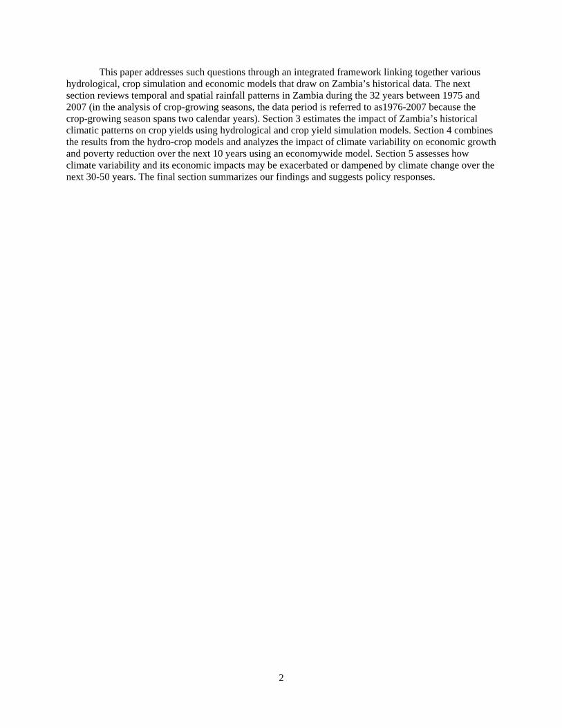
Figure 3 shows the average annual rainfall at the 30 weather stations in Zambia during 1976-2007 interpolated to 1 km pixels. We see a downward gradient of annual rainfall from the north to the south of the country, with the highest rainfall in the northwest and northeast (generally above 1200 mm) and the lowest in the southwest (generally below 800 mm).

1 There is a tradeoff between station coverage and the lengths of observations available from the selected stations. The

choice of data from 30 stations for the period 1975-2007 was thus a balance between cross-sectional and time-series coverage.

4

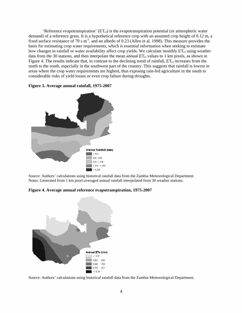
‘Reference evapotranspiration’ (ETO) is the evapotranspiration potential (or atmospheric water demand) of a reference grass. It is a hypothetical reference crop with an assumed crop height of 0.12 m, a fixed surface resistance of 70 s m-1, and an albedo of 0.23 (Allen et al. 1998). This measure provides the basis for estimating crop water requirements, which is essential information when seeking to estimate how changes in rainfall or water availability affect crop yields. We calculate monthly ETO using weather data from the 30 stations, and then interpolate the mean annual ETO values to 1 km pixels, as shown in Figure 4. The results indicate that, in contrast to the declining trend of rainfall, ETO increases from the north to the south, especially in the southwest part of the country. This suggests that rainfall is lowest in areas where the crop water requirements are highest, thus exposing rain-fed agriculture in the south to considerable risks of yield losses or even crop failure during droughts.

Figure 3. Average annual rainfall, 1975-2007

Source: Authors’ calculations using historical rainfall data from the Zambia Meteorological Department. Notes: Generated from 1 km pixel-averaged annual rainfall interpolated from 30 weather stations.

Figure 4. Average annual reference evapotranspiration, 1975-2007

Source: Authors’ calculations using historical rainfall data from the Zambia Meteorological Department.

5

Notes: Generated from 1 km-pixel averaged annual ETo interpolated from ETo values calculated for 30 weather stations.

The main objective of this study is to analyze the impact of climate variability on Zambia’s economy, which relies heavily on agriculture. While detailed spatial information at a more disaggregated level is available for some of the climate-related indicators, and this level of discrimination might be more helpful for an analysis of climate variability, the related social and economic data are not currently available at this level.

To capture certain spatial patterns of climate variability and agricultural production, we first aggregate the country into five agroecological zones. There are four nationally defined agroecological zones, Zone I, Zone IIa, Zone IIb, and Zone III, and we further divide Zone IIa into two subzones, Zone IIa1 and Zone IIa2, because of differences in their rainfall patterns (see below for discussion). Zone I covers most of the Southern province and parts of Lusaka and the Eastern provinces. Zone IIa1 covers the capital city Lusaka and the eastern parts of the Central province, while Zone IIa2 includes the western parts of the Central province and most of the Eastern province. Zone IIb comprises most of the Western province. Finally, Zone III, which is the largest in terms of geographic size, includes the Copperbelt, North Western, Luapula and Northern provinces. In this study, rainfall and other meteorological data are aggregated to these five zones, taking into consideration the influencing domain of each weather station (Figure 2). Zonal-level average annual rainfall is presented in Figure 5, which shows a similar pattern to that found in Figure 3, with the highest rainfall in the northern Zone III, and the lowest rainfall in the southern Zone I. Zone IIa1 has a mean annual rainfall of 818 mm, which is only slightly higher than that of Zone I. In contrast, Zones IIa2 and IIb have higher annual rainfalls, at 941 mm and 930 mm, respectively. These differences emphasize the importance of separating the eastern and western parts of Zone IIa, especially since most of Zambia’s economic activity takes place near Lusaka.2

Figure 5. Average annual precipitation by agroecological zone, 1976-2007 (mm)


Intra-annual distribution and Inter-Annual Variations of Rainfall and Evaporation

The distribution of rainfall and temperatures during a year determines the growing season of annual crops and influences yields, especially those of crops cultivated under rain-fed conditions. Figure 6 shows monthly rainfall distributions in Zambia’s five agroecological zones. In all five zones, most of the rainfall

2 Appendix C describes the economic structure of the five agroecological zones.

6

is concentrated between November and April (the rainy season), with virtually no rainfall from May to September (the dry winter season). Although the 20- to 40-mm rainfall seen in October marks the end of the dry season, the depletion of soil moisture during the dry season may prevent immediate crop planting in this month. While all five zones experience similar rainfall patterns across the seasons, certain within-season differences can be found among the zones. For instance, the January-March rainfall in Zone III is nearly 300 mm higher than that in Zone I. This becomes particularly important when we note that 300 mm of water is close to 50 percent of the water required by some dry land crops.

Figure 6. Mean monthly precipitation by agroecological zone, 1976-2007


Compared to the intra-year distribution of rainfall, the ETO shown in Figure 7 is low during the rainy months and high during the dry months. For all zones, the lowest ETO is seen in December to February (around 100 mm), when the wind speed is lowest and rainfall and relative humidity are highest for the year. The highest ETO values are seen in September, when these values range from a low of about 160 mm in Zone III to a high of 200 mm in Zone IIb. During this month, the temperature and wind speed are highest and the relative humidity is lowest for the year. Interestingly, a second peak of ETO is seen in May in all zones; this is confirmed by the observed open-water pan evaporation data for most of the 30 weather stations. For Zone III, the relative humidity is lower and the wind speed is higher during May compared to those values in April and June, perhaps explaining the small peak of ETO in May. This is not seen in other zones.3

Year-to-year variations in rainfall are generally high in zones with low rainfall and low in wetter zones towards the north. Figure 8 gives the normalized standard deviation (i.e., the coefficient of variation) of annual rainfall for the period 1976-2007. The dry Zones I and IIa1 have the highest inter-annual rainfall variabilities, with coefficients of 0.180 and 0.203, respectively. Assuming that the annual rainfall amount follows a normal distribution, this implies that in Zone IIa1, for example, there is about a 30 percent probability that the rainfall in any given year will be 20 percent (i.e., 170 mm) higher or lower than the mean rainfall level of 820 mm shown in Figure 5. This indicates the potential for moderate drought or flood events, depending on the distribution of the rainfall deficit or surplus in a particular rainy season. A higher coefficient of variation for Zone IIa1 indicates that this zone has a higher inter-annual rainfall variation compared to that in Zone I, despite the latter having a lower average annual rainfall.

3 A thorough explanation of the bimodal intra-year distribution of ETO must await further analysis.

7

Figure 7. Mean monthly reference evapotranspiration in the agroecological zones, 1976-2007


Figure 8. Annual precipitation coefficient of variation by agroecological zone, 1976-2007

Source: Authors’ calculations using historical rainfall data from the Zambia Meteorological Department. Notes: Standard deviation is used to indicate inter-annual variations of rainfall in an agroecological zone.

Figure 9 shows inter-year rainfall variations in each of the five zones, while Figure 10 shows the percent deviations of annual rainfall from their means. The annual dry and wet fluctuations appear to share the same rhythms during major drought and wet years in Zones I, IIa1, IIa2 and IIb, but not in Zone III. This indicates that drought events can be nationwide in some years, making the country less capable of mitigating drought consequences through its own efforts. The wet Zone III shows only moderate inter-year rainfall variation, with rainfall in most years lying within 10 percent of the mean and rarely falling below 1100 mm. In contrast, the rainfall deviations in Zones I, IIa1 and IIb frequently exceed 20 percent of the mean, and approach 30 percent deficits in major drought years.

8

Figure 9. Annual precipitation in the agroecological zones, 1976-2007

Zones I, IIa1 and IIb

Zones IIa2 and III


9

Figure 10. Annual deviation from long-term mean precipitation for the agroecological zones


Zones IIa2 and III


The potential evapotranspiration (ET) values for maize during its growing season are shown in Figure 11.4 Maize is chosen for the discussion because it is Zambia’s most important annual crop. Clearly the amplitudes of the inter-year potential ET variations are much smaller than the rainfall amounts. Nevertheless, as is seen for rainfall, the variations of potential ET are large in Zones I, IIa1 and IIb but small in Zones IIa2 and III. Even for zones with large variations, the difference in maize evapotranspiration between any two years is well within 100 mm (Zone III, it is only around 30 mm). The potential ET for maize during the growing season in each of the zones is found to be inversely correlated with zonal rainfall. The opposite deviations of rainfall and potential ET in the same year are particularly

4 See Appendix A.

10

apparent in major drought years (1986/87, 1991/92, 1994/5 and 2004/05) and major wet years (1977/78, 1988/89, 1992/93 and 2006/07).5 This suggests that larger-than-usual amounts of water are needed by crops during years when rainfall is low. On the other hand, crop water requirements are usually below normal in years when rainfall is high (potentially due to flooding and water-logging).

Figure 11. Growing period potential evapotranspiration of maize in the agroecological zones, 1976-2007


Zones IIa2 and III

Source: Results from the hydro-crop model (see below).

5 The harvest year is usually associated with drought/floods, even though the growing season spans two calendar years. For

example, the drought that took place during the 1991-92 season corresponds to 1992 for the other data sources (e.g., national accounts). We follow this convention when the season is not explicitly identified in the text.

11

Distribution of Droughts and Wet Events Based on Drought Index Analysis

As droughts are complex phenomena, their severity is often measured using an index. For agriculture, drought indices usually take into account the amount of soil water available to crops, rather than focusing solely on rainfall deficits. For this study we use the Palmer Z index (Palmer 1965; Alley 1984), a drought severity metric that out-performs other indicators of monthly soil moisture conditions. The Palmer Z index, which is based on the supply-demand concept of the soil water balance, not only accounts for more than just rainfall deficits at specific locations, it also provides a standardized measure of moisture conditions, thus allowing for comparisons across locations and time periods. Detailed calculation procedures can be found in Palmer (1965).

The annual drought indices discussed below are actually a wet season (November-March) average of the monthly Palmer Z indices, largely because the wet season overlaps with the growing period of most rain-fed crops, including maize. A negative value for the Palmer Z index indicates dry conditions, while a positive value indicates wet conditions. Unfortunately, the monthly meteorological data we use in this study do not provide sufficient information to enable us to identify floods (which usually occur over much shorter periods of time, such as a few days) versus heavy rains (World Bank, 2008). However, the wet conditions indicated by a high positive value of the Palmer Z index might suggest the presence of flooding. Monthly Palmer Z indices are calculated for 1975-2007 for the five agroecological zones, and are then averaged over the wet season to create annual drought indices for each zone for the 1976-2007 harvest years. As shown in Table1, threshold values are chosen for the index, allowing us to categorize the growing seasons into severe drought years (-1.5), moderate drought years (-0.5), normal years, moderately wet years (0.5) and very wet years (1.5). The threshold values are more or less arbitrarily set as described in Palmer (1965). It is worth noting that the original ‘near normal’ range given by Palmer (1965) was -0.49 to 0.49.

Table 1. Number of years of simultaneous climatic event occurrences across agroecological zones, 1976-2007

Number of zones simultaneously

affected

Severe drought

(Za ≤ -1.5)

Moderate drought

(-1.5 < Z ≤ -0.5)

Normal

(-0.5 < Z ≤ 0.5)

Moderately wet

(0.5 < Z ≤ 1.5)

Very wet

(Z > 1.5 )

5 0 1 (1994) 0 0 0

4 0 4 0 4 1 (1978: I, IIa1, IIa2, IIb)

3

1 (1992: I, IIa1, IIb)

4 6 5 0

2

2 (1995: I, IIa1; 2005: I, IIa1)

4 11 2

1 (1981: I, IIb)

1

1 (1987: IIa1)

7

10

9 4 (1979: III; 1989: IIa1; 1997: IIa1; 2004: 2b)

Note a: Values represent the averaged monthly Palmer Z Indices for the maize-growing periods from November to March. The monthly Palmer Z index shows how monthly moisture conditions depart from normal, reflecting short-term drought and wetness (Palmer 1965; Alley 1984).

12

From the perspective of agriculture, a drought’s spatial extent can prove as important as its severity measure. The simultaneous occurrence of drought conditions across large areas can greatly reduce a country’s ability to mitigate negative outcomes and provide food assistance to drought-stricken regions. Table 1, which gives the frequencies of drought/wet events taking place simultaneously across agroecological zones during the 1976-2007 study period, shows that the worst drought events are seen during the 1991/92 growing season, when three out of the five zones experienced severe droughts (i.e., Zones I, IIa1, IIb). Zones I and IIa1 also experienced severe droughts during the 1994/95 and 2004/05 seasons, while Zone IIa1 alone experienced a severe drought in 1986/87. These four periods represent the major drought years in the historical rainfall data.

In Zambia, we see that moderate droughts occur more often than severe droughts and usually affect larger areas. Table 1 shows that all five agroecological zones experienced moderate droughts during the 1993/94 season; this is the only countrywide moderate drought observed in the 32-year period between 1976 and 2007. In addition, there were four other rainy seasons during the study period when four of the five zones were simultaneously affected by moderate droughts; four seasons when three of the five zones were simultaneously affected; and four seasons when two of the five zones were simultaneously affected. It is more common for only one agroecological zone to be under moderate drought conditions; there were seven seasons with moderate droughts in one of the five zones, with a reoccurrence interval of approximately 4.5 years.

‘Normal’ weather (i.e., a Palmer Z index between -0.5 and 0.5) was never simultaneously observed in more than three of the five agroecological zones during the 32-year study period, indicating that Zambia is prone to extreme weather events. There were six seasons when normal weather simultaneously occurred in three of the five zones; eleven seasons when normal weather was seen simultaneously in two zones; and ten seasons when normal weather was seen in only one zone.

Moderately wet and very wet events appear to be less frequent than droughts, and were never experienced by all five zones simultaneously. The indices show four seasons during which moderately wet conditions occurred simultaneously in four of the five zones; five seasons when moderate wet occurred simultaneously in three zones, and two seasons when moderate wet occurred simultaneously in two zones. The chance that only one zone would be moderately wet during a given season was considerably higher (i.e., nine out of a total of 32 years).

Finally, as with severe droughts, very wet conditions rarely occur simultaneously in Zambia. The 1977/78 season was the only period during which four zones (Zones I, IIa1, IIa2 and IIb) simultaneously experienced very wet conditions. Moreover, the 1980/81 season was the only period during which two zones (Zones I and IIb) were simultaneously affected, while only four seasons could be characterized as having a single agroecological zone under very wet conditions.

Some conclusions can be drawn from Table 1. First, Zambia is prone to droughts and floods; there is a high chance that at least one agroecological zone experienced an abnormal weather event in any given year. Second, the central and southern regions of the country (Zones I, IIa1 and IIb) are particularly prone to both droughts and floods, whereas Zone III shows fairly stable weather conditions, with no severe droughts over the last three decades and only one season (i.e. 1978/79) identified as being very wet. Third, it seems that drought events have grown more frequent over time, with almost all of the country’s severe droughts taking place during the second half of the study period.

13

3. MODELING THE BIOPHYSICAL IMPACT OF CLIMATE VARIABILITY USING A HYDRO-CROP MODEL

Two types of models are used to analyze the economic impacts of variability and climate change herein: an integrated hydro-crop model is first used to predict soil water balances and crop yield responses in Zambia’s five agroecological zones, and then this information is applied to an economywide dynamic computable general equilibrium (DCGE) model, which estimates impacts on production at the subsector, zonal and national levels, as well as on household incomes and poverty. This section describes the hydro-crop model and the estimation of crop yield losses resulting from climate variability.

Quantitative data on the responses of crop yields to water deficiency are crucial for evaluating the economic impacts of climate variability and change on agricultural production. In Zambia, the impact of climate variability on agriculture is especially important, given that it is the primary impact channel through which the broader economy is affected (World Bank, 2008). Different approaches may be used to estimate crop yields under varying weather conditions. One approach is to use process-oriented crop growth models to simulate crop growth and yields, taking into account detailed biophysical processes ranging from the extraction of water and nutrients by root systems, to plant photosynthesis and yield formation. However, these kinds of models require extensive soil and crop information, and are typically constructed separately for different crops. Given the lack of data for Zambia, we herein adopt a semi-empirical approach and develop a hydro-crop model that includes two stages. In the first stage, we simulate actual evapotranspiration using a soil water balance model for crop root zones; this is similar to the procedure recommended in Allen et al. (1998). In the second stage, we estimate crop yield responses to water deficits using the empirical crop water production model originally proposed by Jensen (1968). Together, these two stages form our integrated ‘hydro-crop’ model.

The output of the hydro-crop model becomes an input into the economywide DCGE model that we use to assess the economic impact of climate variability. The DCGE model contains information on different sectors, factors and households in each of the five agroecological zones. For example, the model distinguishes among 34 different sectors, half of which are crop and livestock subsectors and the other half are industrial and service subsectors. Production in each agricultural subsector is disaggregated across zones using district-level data provided by the Ministry of Agriculture, Food and Fisheries. We also separate small/large-scale and rural/urban agricultural production. In this way, the model captures differences in cropping and livestock patterns driven by agroecological conditions and farm land endowments. This disaggregation of production allows the DCGE model to capture how climate conditions vary across zones, and how climate affects crops differently according to their agronomic characteristics. The economywide model’s characteristics and simulations are described in detail in Section 4.

The Hydro-Crop Model

The soil water balance module of the hydro-crop model regards the crop’s root zone as a bucket, with water flowing in through rainfall (and irrigation if applicable), and leaking away as evapotranspiration, runoff and deep percolation. The first step in calculating the soil water balance is to estimate crop’s water requirements, which are normally expressed by the rate of potential ET. The United Nation’s Food and Agriculture Organization (FAO) has developed a practical procedure for estimating a crop’s water requirements (Allen et al. 1998), which has become a widely accepted standard. Owing to the difficulty of obtaining readily available and accurate field measurements, estimates of crop water requirements are typically derived from estimates of crop ET for a reference crop (similar to clipped grass) under the relevant climatic conditions. The water requirements of a given crop are thereafter derived through a calculation that integrates the combined effects of crop transpiration and soil evaporation into a single crop coefficient. Details of the soil water balance model and the crop water production model are given in Appendices A and B.

14

There is a rich literature on crop yield responses to water deficits (e.g. Jensen 1968; Doorenbos and Kassam 1979). However, the decision on which crop water production model to use for an economic evaluation is usually constrained by the complex nature of these models and the availability of the necessary parameters. Thus, simpler estimation models, such as the FAO linear yield response model (Doorenbos and Kassam 1979) and Jensen’s model (Jensen 1968), are usually preferred over more complex models.

The FAO model is a practical approach for measuring crop yield responses to water supplies: it is relatively simple; requires commonly available climatic, water, soil and crop data; and is applied widely with acceptable levels of accuracy.6 However, the FAO linear model for the total growing period does not work well for Zambia; a comparison of observed yields versus FAO model simulations suggests that crop losses in the country are especially sensitive to seasonal water deficits. Therefore, it is not appropriate to apply this model, which uses relative evapotranspiration for the entire growing season and thus cannot capture monthly climate variations and crop yield sensitivities, which are critical in Zambia. Yield response factors for individual growing periods are available from the FAO (1979), and may be used to assess yield losses due to water deficits in an individual crop-growing period. However, there is no detail discussion in the method in the FAO study for how to use these factors conjunctively to assess yield loss due to water deficits in multiple growing periods. Therefore, we use the Jensen crop water production model7 and estimate the necessary crop water sensitivity index values based on FAO yield response factors for individual growing periods throughout the growing season (FAO 1979). These estimates are then mapped to each month of the relevant crops’ growing periods using the cumulative sensitivity index method (Tsakiris 1982; Kipkorir, 2002). Figure 12 shows the monthly crop water sensitivity indices for maize, sorghum and root crops.

Figure 12. The crop water sensitivity index from the Jensen crop water production functions for maize, sorghum and root crops. The vertical axis is the crop water sensitivity index, which is dimensionless.

Impact of Climate Variability on Crop Yields: Hydro-Crop Model Results

Figure 13 shows the simulated ET for the maize growing season in the five agroecological zones. Affected simultaneously by crop water requirements and soil moisture contents, the plots showing actual evapotranspiration in the three drier zones (Zones I, IIa1 and IIb) reveal the presence of rising and falling

6 Equation 2.8 in Appendix A. 7 Equation 2.9 in Appendix A.

15

patterns similar to the rainfall patterns shown in Figure 9. This is because the limiting factor in these zones is the available soil water content. However, the actual evapotranspiration patterns in the wetter zones (Zones IIa2 and III) follow the potential evapotranspiration patterns shown in Figure 11, because the soil water content does not constrain evapotranspiration in these zones (instead, it is controlled by the atmospheric water demand).

Figure 13. Growing period actual evapotranspiration of maize in the agroecological zones, 1976-2007


Zones IIa2 and III

Source: Results from the hydro-crop model.

16

Simulated relative maize yields for 1976-2007 are shown in Figure 14 for the five agroecological zones. Relative yields are defined as the ratio of the simulated actual yield to the maximum yield achievable without any water stress. Maize is again chosen as an illustrative example because it is Zambia’s major crop. However, the relative yields for the other major crops follow patterns similar to those of maize.

Figure 14. Maize relative yields in the agroecological zones, 1976-2007 (you need to change the second word with lower case, i.e. Relative yield


Zones IIa2 and III


17

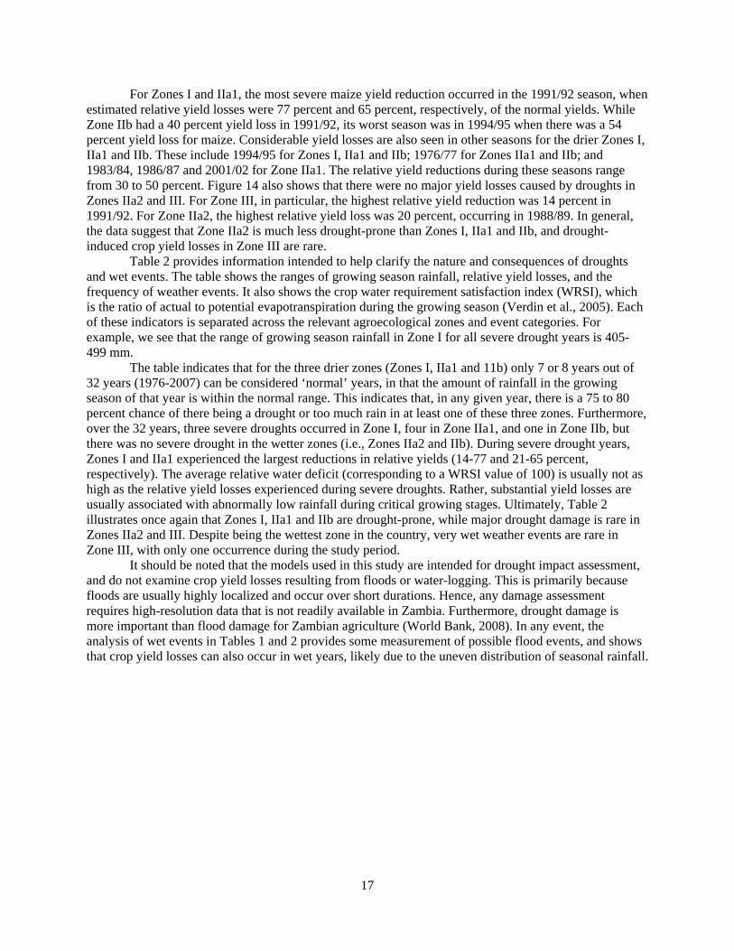
For Zones I and IIa1, the most severe maize yield reduction occurred in the 1991/92 season, when estimated relative yield losses were 77 percent and 65 percent, respectively, of the normal yields. While Zone IIb had a 40 percent yield loss in 1991/92, its worst season was in 1994/95 when there was a 54 percent yield loss for maize. Considerable yield losses are also seen in other seasons for the drier Zones I, IIa1 and IIb. These include 1994/95 for Zones I, IIa1 and IIb; 1976/77 for Zones IIa1 and IIb; and 1983/84, 1986/87 and 2001/02 for Zone IIa1. The relative yield reductions during these seasons range from 30 to 50 percent. Figure 14 also shows that there were no major yield losses caused by droughts in Zones IIa2 and III. For Zone III, in particular, the highest relative yield reduction was 14 percent in 1991/92. For Zone IIa2, the highest relative yield loss was 20 percent, occurring in 1988/89. In general, the data suggest that Zone IIa2 is much less drought-prone than Zones I, IIa1 and IIb, and drought-induced crop yield losses in Zone III are rare.

Table 2 provides information intended to help clarify the nature and consequences of droughts and wet events. The table shows the ranges of growing season rainfall, relative yield losses, and the frequency of weather events. It also shows the crop water requirement satisfaction index (WRSI), which is the ratio of actual to potential evapotranspiration during the growing season (Verdin et al., 2005). Each of these indicators is separated across the relevant agroecological zones and event categories. For example, we see that the range of growing season rainfall in Zone I for all severe drought years is 405-499 mm.

The table indicates that for the three drier zones (Zones I, IIa1 and 11b) only 7 or 8 years out of 32 years (1976-2007) can be considered ‘normal’ years, in that the amount of rainfall in the growing season of that year is within the normal range. This indicates that, in any given year, there is a 75 to 80 percent chance of there being a drought or too much rain in at least one of these three zones. Furthermore, over the 32 years, three severe droughts occurred in Zone I, four in Zone IIa1, and one in Zone IIb, but there was no severe drought in the wetter zones (i.e., Zones IIa2 and IIb). During severe drought years, Zones I and IIa1 experienced the largest reductions in relative yields (14-77 and 21-65 percent, respectively). The average relative water deficit (corresponding to a WRSI value of 100) is usually not as high as the relative yield losses experienced during severe droughts. Rather, substantial yield losses are usually associated with abnormally low rainfall during critical growing stages. Ultimately, Table 2 illustrates once again that Zones I, IIa1 and IIb are drought-prone, while major drought damage is rare in Zones IIa2 and III. Despite being the wettest zone in the country, very wet weather events are rare in Zone III, with only one occurrence during the study period.

It should be noted that the models used in this study are intended for drought impact assessment, and do not examine crop yield losses resulting from floods or water-logging. This is primarily because floods are usually highly localized and occur over short durations. Hence, any damage assessment requires high-resolution data that is not readily available in Zambia. Furthermore, drought damage is more important than flood damage for Zambian agriculture (World Bank, 2008). In any event, the analysis of wet events in Tables 1 and 2 provides some measurement of possible flood events, and shows that crop yield losses can also occur in wet years, likely due to the uneven distribution of seasonal rainfall.

18

Table 2. Palmer Z drought index-based weather classification and the ranges of derived climatic and agronomic statistics, 1976-2007

Severe drought year

(Za ≤ -1.5)

Moderate drought year

(-1.5 < Z ≤ -0.5)

Normal year

(-0.5 < Z ≤ 0.5)

Moderately wet year

(0.5 < Z ≤ 1.5)

Very wet year

(Z > 1.5)

Zone I Growing period rainfall (mm) 405-499 481-624 632-751 746-902 971-1031 Maize WRSIb (%) 70-96 94-100 96-100 97-100 100

Maize yield lossc (%) 14-77 1-15 0-8 0-10 0

Frequencyd 3 8 8 11 2

Zone IIa1 Growing period rainfall (mm) 401-506 505-623 711-781 761-887 961-1008 Maize WRSI (%) 75-95 83-100 94-100 92-100 96-100

Maize yield loss (%) 21-65 0-48 7-19 1-23 0-14

Frequency 4 9 7 9 3

Zone IIa2 Growing period rainfall (mm) - 635-781 765-954 910-1058 1113e Maize WRSI (%) - 97-100 95-100 95-100 99

Maize yield loss (%) - 1-11 0-17 0-20 2

Frequency - 11 10 10 1

Zone IIb Growing period rainfall (mm) 585 578-766 765-858 927-1085 1079-1125 Maize WRSI (%) 86 86-100 88-100 95-100 97-100

Maize yield loss (%) 40 0-44 1-34 0-21 0-10

Frequency 1 13 7 8 3

Zone III Growing period rainfall (mm) - 875-987 960-1158 1136-1314 1290 Maize WRSI (%) - 98-100 97-100 100-100 100

Maize yield loss (%) - 0-9 0-13 0-0 0

Frequency - 7 18 6 1 Notes: (a) Average monthly Palmer Z Index during maize-growing period (November-March). The Palmer Z index shows how monthly moisture deviates from normal conditions and reflects short-term drought or wetness (Palmer 1965; Alley 1984). (b) ‘WRSI’ stands for ‘water requirement satisfaction index’ and is the ratio of total actual to total potential crop evapotranspiration (see Section 2). (c) Percentage maize yield loss is estimated from the hydrological model. (d) Number of years of occurrences during 1976-2007. Using the monthly averaged Palmer Z index and the -1.5 threshold, we did not identify year 1992 as a severe drought year in Zone I, even though the estimated maize yield reduction calculated herein (about 77 percent) was the most severe among the five agroecological zones. In contrast, the index successfully identified the other severe drought years (1995 and 2005) for Zone I. This is because Zone I received only 22 mm of rainfall in February 1992, which is about 13 percent of the rainfall average for this month. This extreme rainfall shortage, which occurred during a critical maize-growing stage, resulted in dramatic yield losses in 1992. To correct for this discrepancy, we moved 1992 from the ‘moderate’ to ‘severe’ drought category for Zone I. (e) Only one very wet event was seen in Zone IIa2 during the 1976-2007 period, and hence we did not report it. The same is true for severe drought in Zone IIb and very wet events in Zone III.

19

4. CLIMATE VARIABILITY AND ECONOMIC GROWTH: COMBINING THE HYDRO-CROP AND DCGE MODELS

The previous sections examined historical trends in climate variability across Zambia’s five major agroecological zones (Section 2) and estimated their annual impact on crop yields over the past three decades using a hydro-crop model (Section 3). Drawing on the hydro-crop model results and climate variability data, this section assesses the potential impact of future climate variability on economic growth, household incomes and poverty using the DCGE model developed for this study.

The dynamic computable general equilibrium (DCGE) model

Climate variability not only affects crop yields, harvested areas, and agricultural production, it also has implications for the entire economy. Moreover, spatial variation in rainfall patterns means that such effects can vary across subnational regions. We therefore develop an economywide model with five agroecological zones.8 The model contains detailed information on production, consumption and trade, and includes 34 different production sectors, half of which are agricultural crops and livestock. These sectors are defined for the five agroecological zones (considered as five representative rural farm groups), as well as for large-scale and urban farm groups. The technologies of these representative farm groups (together with the nonagricultural production functions) are calibrated using district-level production data from the Crop Forecasting Surveys (CFS) and the 2004 Living Conditions Monitoring Survey (LCMS4) obtained from Zambia Ministry of Agriculture and Statistic Bureau. Each farm group can change its cropping and livestock patterns and engage more or less intensively in nonfarm activities. Laborers can also migrate to urban centers and nonagricultural jobs (both are modeled explicitly). This model therefore captures some autonomous adaptation to climate change. However, we limit the extent to which representative producers adjust cropping patterns in response to short-term climate variability. We assume that land allocations are determined at the start of the season, and that farmers cannot reallocate planted land to different crops during the growing season (i.e., land allocations are exogenous in the short-run). This assumption is appropriate, since farmers typically cannot predict or respond to climate variation once land is planted. They can, however, reallocate mobile resources (e.g., labor) and influence the level of production.

While substitution between factors (labor, land and capital) depends on relative costs, the model distinguishes among self-employed agricultural workers, unskilled workers (working in both agriculture and nonagriculture), and skilled workers (in nonagriculture only). Information on employment and wages is from the LCMS4, while labor supplies are allowed to exogenously expand over time according to demographic projections. Capital is immobile across sectors, and, after accounting for annual depreciation, is supplemented by past investments allocated according to each sectors’ relative profitability. This is the ‘recursive’ dynamic feature of the DCGE model. Total factor inputs are then combined with intermediate inputs (e.g., fertilizer and fuels) to produce a total level of output. These sector-specific production technologies are taken from a 2006 Zambian social accounting matrix (SAM). Producers in each sector/region decide how much output to supply to the national domestic and foreign markets based on relative prices. Since Zambia is a small country, we assume that world prices are fixed, but also that they are influenced by changes in the real exchange rate, which adjusts to maintain the current account balance.

In order to capture how different households are affected by climate variability and change, the model includes 15 representative household groups; these are separated by zone, by rural or urban location, and by farm size (e.g., small-scale rural, large-scale rural and urban farmer households). Income and expenditure patterns vary across the 15 household groups. This is important for modeling distributional change, since incomes generated during farm/nonfarm production accrue to different households depending on their location and factor endowments. Households in the model receive factors’

8 The equations and parameters of the DCGE model are presented in Appendix D.

20

incomes, and then pay taxes, save and make transfers to other households. The remaining income is used to consume goods and services, which can either be purchased locally or imported, depending on relative prices. Taxes are collected by the government, which also consumes goods and services, while pooled savings are used to finance investment spending. Total demand interacts with production and trade (i.e., supply) to determine prices. This full specification of supply/demand for commodities and the factors using the production and utility functions is the ‘general equilibrium’ feature of the DCGE model. Finally, in order to retain as much information as possible on the households’ incomes and expenditure patterns, the DCGE model is linked to a microsimulation module based on the LCMS4. Changes in consumption for each representative household in the DCGE model are used to adjust the level of commodity expenditure of the corresponding household in the LCMS4. The consumption levels are then recalculated in the survey, and standard poverty measures are re-estimated.

The model distinguishes domestic markets from trade with rest of world for the most important trading commodities. However, international prices can affect domestic supply and demand through imperfect substitution with domestic supply, as well as through the real exchange effect. The linkages among different agricultural subsectors and between agricultural and nonagricultural sectors are fully captured through income generation, household expenditures, and the use of intermediate inputs. In this way, the economywide impacts of climate variability in Zambia can be captured. The detailed data used to represent the Zambian economy in 2006, as well as the macroeconomic and sectoral structure of the production, are taken from national accounts and crop production data, while data on household incomes and expenditures are drawn from the LCMS4. Note that the agricultural season used for the calibrated base year of the model is 2005/06. Appendix C provides a detailed description of the DCGE model for Zambia.

Combining the Hydro-Crop and DCGE Models: Designing Scenarios Representing Alternative Rainfall Patterns

The DCGE model is used to simulate the 10-year climate variability between 2006 and 2016 and to assess the economic impact of this variability. It is impossible to accurately predict Zambia’s future annual rainfall pattern. It is, however, possible to identify a range of possible patterns using historical data and a variety of methods developed to simulate future potential rainfall patterns. Here, we use an 'index sequential’ method (Prairie et al., 2006). Given 32 years of historical rainfall data for the period 1976-2007, we can draw 32 different rainfall patterns each of which has 10 years to corresponding to simulating period of 2007-2016 (i.e., 32 different starting years chosen from years of 1976-2007 with 10 consecutive years to form a sequence). This method preserves the original inter-annual rainfall patterns inherent in the observed climate data of 1976-2007. We include all 32 of the possible 10-year rainfall patterns in our analysis, thereby capturing the full distribution of past climate variability. This approach has the advantage of greatly reducing the number of possible rainfall scenarios, while also capturing any interdependencies of rainfall patterns across consecutive years.

Thus, the starting point (or the base year) of the DCGE model is 2006, which is the most recent year for which all of the necessary data are available. We first apply the DCGE model to a scenario with ‘normal’ rainfall pattern for the 10 years between 2007 and 2016 (i.e., during the simulated 10 years there are no adverse effects from climate variability on the economy). Because of this insulation from climate variability, crop yields are assumed to be stable. Moreover, yield levels and land allocation are assumed to grow steadily according to estimated yield potentials drawn from field trials and historical trends in land expansion, respectively (see Thurlow et al., 2008). We call this scenario ‘normal rainfall without climate variability’ (or ‘normal rainfall’). We then develop 32 scenarios (each with a period of 10 years) to simulate the economic impact of the different rainfall patterns discussed above. The various rainfall patterns and the economywide model are linked through the imposition of crop yield shocks in the model. These yield shocks are consistent with the Hydro-crop model results discussed in the previous section, and are applied on a crop-by-crop basis for each of the five agroecological zones. This procedure is repeated for all 32 scenarios, each of which is for the period of 10 years. As farmers are unable to predict

21

rainfall patterns and droughts often occur after planting, farmers are usually unable to change land allocation to avoid drought-induced yield loss. Accordingly, in the model we assume that land allocation within each year is fixed by crop. Given that more than 80 percent of the rain-fed crop areas in Zambia are planted with maize, and drought-resistant crops, such as cassava and sorghum, have significant spatial patterns, this assumption seems to be more reasonable than the flexible land allocation assumption that is commonly used in many other CGE models. However, although farmers are unable to reallocate land to other crops, they can reallocate other inputs (e.g., labor, capital and intermediate inputs) in response to climate variability. For example, they may switch labor and capital to other agricultural and nonagricultural activities (e.g., by participating in off-farm activities as workers) in response to drought-induced changes in agricultural prices and nonagricultural employment opportunities.

Apart from imposing the yield shocks drawn from the crop model, we also account for other transmission channels through whic1h extreme rainfall variation can affect the agricultural sector and the rest of the economy. These additional non-yield impacts, which only occur when there is a severe drought or flood event,9 are summarized in Table 3.

Table 3. Climate variability and severe drought/flood event impact channels assumed in the economywide model

Impact channel Affected sectors Description of impact

All 10 years in each of the 32 scenarios

Crop yields Rain-fed crops Level of yield reduced based on the crops’ WRSI

Years with severe drought events that reflect rainfall patterns in 1983/84, 1986/87, 1991/92, 1994/95 and 2001/02

Crop area expansion Rain-fed crops Crop land expansion that would take place in a normal year is eliminated in the drought year and remains at zero in the immediate post-drought year

Livestock stocks Livestock sectors Livestock stocks decline in the drought year and the growth in these stocks gradually returns to normal year rates over the two subsequent years, with diminishing lagged effects

Physical capital accumulation All sectors Capital depreciation rates are increased in the drought year and gradually return to normal year levels over the two subsequent years, with diminishing lagged effects

Major flood year (2006/07)

Agricultural land expansion Crop sectors Land area under cultivation declines in the flood year, then returns to pre-flood levels in the immediate post-flood year

Note: ‘WRSI’ is water response satisfaction index (see Section 2.3). Details of each impact channel are provided in Appendix A.

9 Major drought events are defined for a particular agro-climatic zone as being years in which the WRSI index is two

standard deviations or more below the mean for the period of 32 years (1976-2007). For Zone IIa1 this occurred in the following seasons: 1983/84, 1986/87, 1991/92, 1994/95 and 2001/02. Due to a lack of data to support the modeling of floods, only the 2007/08 season is herein identified as a major flood event.

22

Climate variability can also affect the harvested crop areas. Compared to the ‘normal’ scenario, the harvested areas for drought-affected crops are reduced in severe drought years and then slowly recover over the subsequent two years, reflecting a post-drought recovery period. Similarly, cultivated land area also declines during a major flood event, thereby reflecting the situation observed in reality (World Bank, 2008). Livestock stocks and the productivity of livestock production are also affected by a severe drought.10 The recovery of livestock stocks to normal levels is assumed to take about two years. Thus, there is a lagged but diminishing effect on livestock stocks and productivity in the second and third years following a severe drought or flood. Severe drought is also assumed to affect other types of physical capital through a higher than normal depreciation rate. This reflects deterioration or greater underutilization of capital stocks. As with livestock stocks, there is a lagged effect on the recovery of the capital depreciation rate following a severe drought or flood, with the depreciation rate returning to its normal-year levels over a two-year period. Thus, while crop yield losses are the primary impact channel, the economywide model also captures numerous other possible channels through which climate variability and extreme drought/flood events can affect production and productivity in both agricultural and nonagricultural sectors.

Economywide Impacts of Climate Variability: DCGE Model Results

Climate Variability will Cost Zambia US$4.3 Billion in Foregone GDP over 10 Years

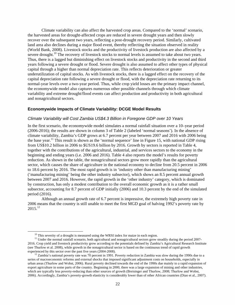
In the first scenario, the economywide model simulates a normal rainfall situation over a 10–year period (2006-2016); the results are shown in column 3 of Table 2 (labeled ‘normal seasons’). In the absence of climate variability, Zambia’s GDP grows at 6.7 percent per year between 2007 and 2016 with 2006 being the base year.11 This result is shown as the ‘normal sequence’ line in Figure 15, with national GDP rising from US$10.2 billion in 2006 to $US19.6 billion by 2016. Growth by sectors is reported in Table 4, together with the contributions of the agricultural, industrial, and services sectors to the economy in the beginning and ending years (i.e. 2006 and 2016). Table 4 also reports the model’s results for poverty reduction. As shown in the table, the nonagricultural sectors grow more rapidly than the agricultural sector, which causes the share of agriculture in the national economy to decline from 20.5 percent in 2006 to 18.6 percent by 2016. The most rapid growth is in ‘industry other than manufacturing mining’ (‘manufacturing mining’ being the other industry subsector), which shows an 8.5 percent annual growth between 2007 and 2016. However, the rapid growth in the ‘other industry’ category, which is dominated by construction, has only a modest contribution to the overall economic growth as it is a rather small subsector, accounting for 8.7 percent of GDP initially (2006) and 10.3 percent by the end of the simulated period (2016).

Although an annual growth rate of 6.7 percent is impressive, the extremely high poverty rate in 2006 means that the country is still unable to meet the first MGD goal of halving 1992’s poverty rate by 2015.12

10 This severity of a drought is measured using the WRSI index for maize in each region. 11 Under the normal rainfall scenario, both agricultural and nonagricultural sectors grow steadily during the period 2007-

2016. Crop yield and livestock productivity grow according to the potentials defined by Zambia’s Agricultural Research Institute (see Thurlow et al. 2008), while growth in the nonagricultural sector is based on the continuous trend of rapid growth experienced by this sector over the past five years (2004-2008).

12 Zambia’s national poverty rate was 70 percent in 1991. Poverty reduction in Zambia was slow during the 1990s due to a series of macroeconomic reforms and external shocks that imposed significant adjustment costs on households, especially in urban areas (Thurlow and Wobst, 2006). Rural poverty declined towards the end of the 1990s due mainly to a rapid expansion of export agriculture in some parts of the country. Beginning in 2000, there was a large expansion of mining and other industries, which are typically less poverty-reducing than other sources of growth (Breisinger and Thurlow, 2008; Thurlow and Wobst, 2006). Accordingly, Zambia’s poverty-growth elasticity is considerably lower than of other African countries (Diao et al., 2007).

23

Table 4. Growth and poverty outcomes under the normal rainfall scenario, 2007-2016

Average annual growth rate, 2007-2016 (%)

Share of total GDP (%) 2006 2016

Gross domestic product (GDP) 6.7 100.0 100.0 Agriculture 5.7 20.5 18.6 Mining 5.9 10.1 9.4 Manufacturing 7.3 12.1 12.8 Other industries 8.5 8.7 10.3 Services 6.7 48.6 48.9

Share of total population, 2006 (%)

Poverty headcount (%) 2006 2016

Poverty headcount 100.0 67.9 52.2 Rural 60.9 77.6 63.0 Urban 39.1 52.8 35.4

Source: Results from the Zambian DCGE model.

We then simulate 32 different rainfall patterns derived from the historical rainfall data using the index sequential method described in Section 3.2. Obviously, climate variability is expected to reduce the growth in GDP through the various impact channels discussed above. The extent of GDP reduction varies across the different rainfall scenarios, which reflect all possible 10-year sequential patterns drawn from the historical rainfall data. To assess the potential losses in GDP due to climate variability, it is not necessary to display all of the results from these 32 scenarios. Instead, we herein report the mean results across the 32 different scenarios, together with the results from the ‘worst rainfall’ scenario, which is defined later in this section.

The mean GDP level averaged across all 32 rainfall scenarios is shown as the ‘sequence average’ in Figure 15.13 When we project forward all possible 10-year historical rainfall patterns, we see that climate variability may reduce Zambia’s GDP by US$0.8 billion by the end of the 10-year period in 2016 (measured in 2006 prices). The size of Zambia’s economy is therefore 4 percent smaller by 2016 than it would have been in the same year without climate variability. The accumulated GDP losses due to climate variability over the 10-year period (2007-2016) reach US$4.3 billion. This is equivalent to lowering Zambia’s annual GDP growth by 0.4 percent points each year between 2007 and 2016.

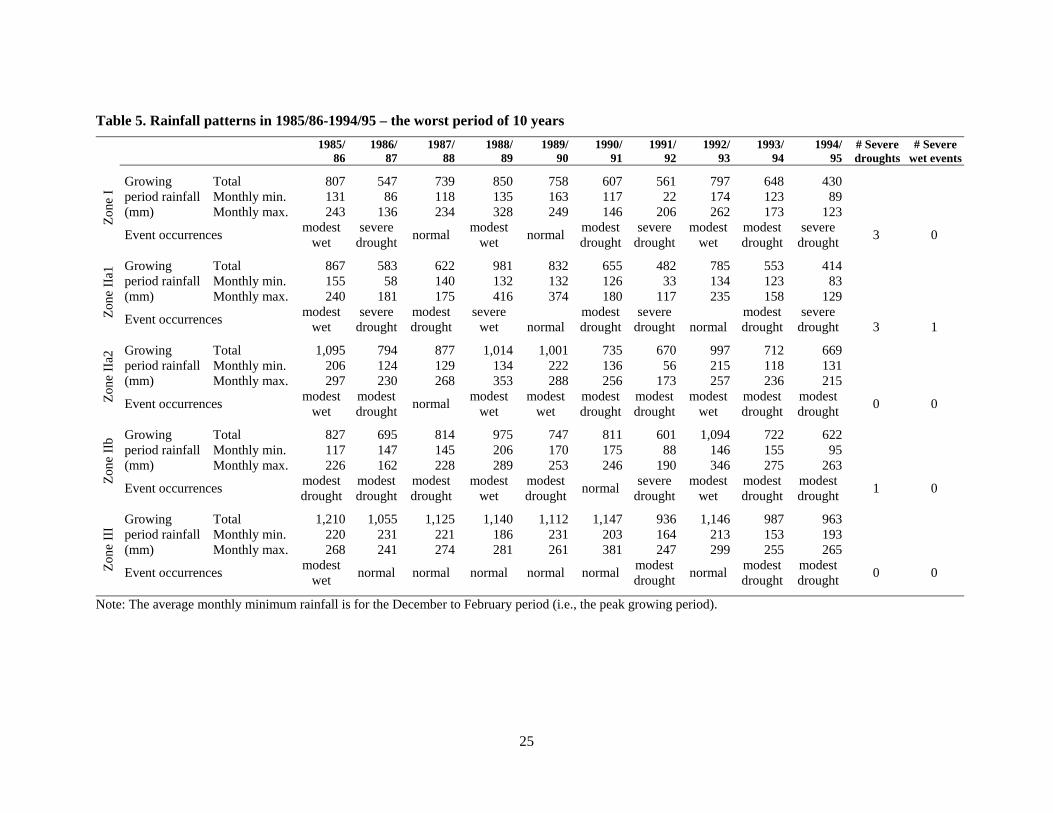
We identify the worst rainfall scenario as the 10-year period having the highest annual precipitation coefficient of variation (CV) and the highest number of severe drought events; this corresponds to the historical rainfall patterns of 1986-1995. Table 5 summarizes the rainfall patterns of this period and shows that the three most severe drought events all occurred during this 10-year period in the scenario (see also Tables 1 and 2 for further details).

The DCGE model simulation shows that if the rainfall patterns over Zambia’s next 10 years replicate the worst rainfall patterns of 10 sequencing years in the history of 1976-2007, then the accumulated total losses in GDP would be US$7.1 billion over the 10-year period of 2007-2016. This is almost twice the mean accumulated losses averaged from all of the possible rainfall patterns discussed above, and is equivalent to reducing Zambia’s annual GDP growth by 0.9 percentage points each year. Moreover, the Zambian economy would be 8.1 percent smaller by 2016 under these conditions than it would have been under a normal rainfall scenario. In other words, total the GDP in 2016 would be US$1.6 billion below what it would have been without any climate variability.

13 To simplify the charts shown in the figure, we do not display the level of GDP under all 32 rainfall scenarios and only

report the mean GDP of these 32 scenarios, the GDP under the worst rainfall scenario, and a few other results for illustrative purposes.

24

Figure 15. Losses in total GDP due to climate variability, 2007-2016

Note: Ten-year losses are the cumulative losses for the entire 2007-2016 period.


Climate variability therefore has a profound effect on economic growth in Zambia, and the losses

associated with the worst rainfall scenario in Zambia’s history are substantial. As the economic losses associated with climate variability are assessed based on historical rainfall data, it is possible for us to apply the model results to the past GDP performance observed during 1976-2007. If climate variability had not caused GDP growth to fall by 0.4 percentage points annually across 1976-2007, then Zambia’s economy, measured by GDP, would have been US$1.5 billion (or 12.8 percent) higher than its actual value (in 2006, given in 2006 prices). In other words, on average, Zambia lost 0.4 percent of growth annually between 1977 and 2007 due to climate variability, and the accumulated cost for this period was US$13.8 billion (in 2006 prices). Thus, while Zambia has indeed undergone several decades of unsuccessful policies and substantial structural reforms, and has suffered from a number of large external shocks that resulted in huge economic costs and decreased growth, climate variability has contributed significantly to the country’s poor economic performance and lowered economic growth, even over the past decade when development has proven more successful.

9.5

11.5

13.5

15.5

17.5

19.5

2006 07 08 09 10 11 12 13 14 15 16

Value in

Billions of 2006 US dollars

Normal sequence

Worst sequence

Sequence average

Total GDP

Average ten‐year loss : US$4.3 bil.Change in growth rate : ‐0.43%

Worst ten‐year loss : US$7.1 bil.Change in growth rate : ‐0.90%

25

Table 5. Rainfall patterns in 1985/86-1994/95 – the worst period of 10 years

1985/

861986/

87 1987/

88 1988/

891989/

90 1990/

91 1991/

92 1992/

93 1993/

94 1994/

95# Severe droughts

# Severe wet events

Zon

e I

Growing period rainfall (mm)

Total 807 547 739 850 758 607 561 797 648 430 Monthly min. 131 86 118 135 163 117 22 174 123 89 Monthly max. 243 136 234 328 249 146 206 262 173 123

Event occurrences modest

wet severe

droughtnormal

modest wet

normal modest drought

severe drought

modest wet

modest drought

severe drought

3 0

Zon

e II

a1 Growing

period rainfall (mm)

Total 867 583 622 981 832 655 482 785 553 414 Monthly min. 155 58 140 132 132 126 33 134 123 83 Monthly max. 240 181 175 416 374 180 117 235 158 129


wet severe

droughtmodest drought

severe wet normal

modest drought

severe drought normal

modest drought

severe drought 3 1

Zon

e II

a2 Growing

period rainfall (mm)

Total 1,095 794 877 1,014 1,001 735 670 997 712 669 Monthly min. 206 124 129 134 222 136 56 215 118 131 Monthly max. 297 230 268 353 288 256 173 257 236 215


wet modest drought

normal modest

wet modest

wet modest drought

modest drought

modest wet

modest drought

modest drought

0 0

Zon

e II

b Growing period rainfall (mm)

Total 827 695 814 975 747 811 601 1,094 722 622 Monthly min. 117 147 145 206 170 175 88 146 155 95 Monthly max. 226 162 228 289 253 246 190 346 275 263

Event occurrences modest drought

modest drought

modest drought

modest wet

modest drought

normal severe

drought modest

wet modest drought

modest drought

1 0

Zon

e II

I

Growing period rainfall (mm)

Total 1,210 1,055 1,125 1,140 1,112 1,147 936 1,146 987 963 Monthly min. 220 231 221 186 231 203 164 213 153 193 Monthly max. 268 241 274 281 261 381 247 299 255 265


wet normal normal normal normal normal

modest drought

normal modest drought

modest drought

0 0

Note: The average monthly minimum rainfall is for the December to February period (i.e., the peak growing period).

26

Climate Variability Lowers Agricultural Growth by 1 Percent Point Each Year

As expected, climate variability has a much larger negative impact on agricultural performance than on overall economic growth. Figure 16 shows the impact of climate variability on agricultural GDP. Under the normal rainfall scenario, agricultural GDP rises from US$2.1 billion in 2006 to US$3.6 billion by 2016 with a 5.7 percent annual growth rate (see Table 4). Because agricultural GDP growth is lower than total GDP growth (5.8 percent) agriculture’s share of GDP falls from 20.4 to 18.6 percent during 2007-16 under the normal rainfall scenario. However, this gradual decline in the importance of agriculture is still fairly optimistic given that this sector that is the most vulnerable to climate variability. The results from the DCGE model reveal the high sensitivity of agricultural GDP to varying rainfall patterns. On average, climate variability causes a total loss in agricultural GDP of US$2.2 billion over the 10-year period. This is equivalent to an annual 1 percent point reduction in agriculture’s growth rate. With this decrease in the annual growth rate, the agricultural GDP in 2016 will be US$0.3 billion below what it would have been under the normal rainfall scenario. Thus, climate variability greatly reduces Zambia’s chances of achieving its national agricultural growth target of 6 percent per year, as set by the Comprehensive African Agricultural Development Program (CAADP).14 As agriculture is particularly vulnerable to climate variability, losses in agricultural GDP account for more than half of the overall projected economic losses, even though the sector comprises only one fifth of the economy.

Figure 16. Losses in agricultural GDP due to climate variability, 2007-2016

Note: Ten-year losses are cumulative for the entire 2007-2016 period, and do not just represent the loss in the final year. Source: Results from the Zambian DCGE model.

Agricultural losses are especially severe under the worst rainfall scenario, which replicates the rainfall patterns of the 10-year period between 1985/86 and 1994/95. If these rainfall patterns were to repeat themselves over the next 10 years (between 2007 and 2016), then the accumulated agricultural GDP losses would amount to US$3.1 billion. This means that under the worst scenario, agricultural GDP is 10.2 percent lower than it would have been under the normal scenario. This is a substantial contraction

14 CAADP, which is an initiative of the New Economic Partnership for African Development (NEPAD), is a compact

among African countries to promote agricultural development and poverty reduction. Zambia will soon become a signatory (see Thurlow et al., 2008).

1.5

2.0

2.5

3.0

3.5

4.0

2006 07 08 09 10 11 12 13 14 15 16

Value in


Normal sequence

Worst sequence

Sequence average

Agricultural GDP

Average ten‐year loss : US$2.2 bil.Change in growth rate : ‐1.01%

Worst ten‐year loss : US$3.1 bil.Change in growth rate : ‐2.29%

27

of the agricultural sector and reflects the severity of the three droughts that took place during 1985-1995. Under the worst rainfall scenario, agriculture’s average annual GDP growth rate during 2007-2016 would be 2.3 percentage points lower than that under the normal rainfall scenario. Such a large decline in agricultural production would severely undermine the country’s development efforts.

Eighty-five Percent of the National Agricultural GDP Losses Caused by Climate Variability Occur in Zones I and IIa1

As examined in Section 2, there is considerable variation in rainfall across Zambia’s five agroecological zones. By disaggregating the country into five different zones, the economywide model is able to capture spatial variation in the economic losses caused by climate variability. Similarly, the zonal-level contribution to the national agricultural economy varies significantly across the five zones. Table 6 reports the zonal shares of agricultural GDP and national maize production, a sector that is particularly vulnerable to climate shocks. Drought-prone Zones I and IIa are an important part of Zambia’s agricultural economy, generating more than half of national agricultural GDP, and almost two-thirds of national maize production.

Table 6. Agricultural GDP and national maize production by agroecological zone, 2006

Agricultural GDP Maize production Value (US$ mil.) Share (%) Level (1000 mt) Share (%)

National 2,095 100.0 1,368 100.0

Zone I 128 6.1 169 12.3 Zone IIa1 1,016 48.5 692 50.6 Zone IIa2 174 8.3 179 13.1 Zone IIb 5 0.3 24 1.7 Zone III 474 22.6 304 22.2

Forestry 297 14.2 - -

Note: The Zambian model does not disaggregate the forestry sector across zones.

Source: 2006 Zambian SAM and the DCGE model.

Zones 1 and IIa1, which represent a relatively large share of national maize production, experience high climate variability. Thus, agriculture in these zones often suffers significantly from bad rainfall patterns. This phenomenon is captured in Figure 17, which separately presents the agricultural GDP growth paths for three selected zones: the two with the highest climate variability (Zones I and IIa1) versus the one with the lowest climate variability (Zone III). The accumulated losses for zonal-level agriculture are, on average, US$0.17 billion in Zone I, which had the smallest agricultural GDP of US$0.14 billion in 2006. The accumulated losses are US$1.68 billion for Zone IIa1, which had an initial agricultural GDP of more than US$1 billion. In contrast, even though agricultural GDP is about US$0.5 billion in Zone III, the accumulated losses due to climate variability in this zone are only US$0.16 billion, which is considerably smaller than those for Zone IIa1 (see Figure 17). This means that almost 85 percent of the national agricultural GDP loss occurs in Zones I and IIa1, whereas Zone III is relatively unaffected by climate variability. Higher climate variability also transfers into lower zonal economic growth rates. While growth in national agricultural GDP is, on average, 1 percentage point lower due to climate variability, larger declines in agricultural growth occur in Zones I and IIa1 (1.3 and 1.6 percentage points, respectively), and a more modest decline is seen in Zone III (0.37 percentage points). Table 7, which summarizes the spatial distribution of the costs of climate variability for all five agroecological zones, clearly shows that the economic cost of climate variability falls heavily on Zambia’s southern and central zones and declines rapidly to the north.

28

Figure 17. Losses in agricultural GDP in Zones I, IIa1 and III due to climate variability, 2007-2016

Note: Ten-year losses are cumulative for the entire 2007-2016 period, and do not just represent the loss in the final year.


0.00

0.05

0.10

0.15

0.20

0.25

2006 07 08 09 10 11 12 13 14 15 16

Value in

Billions of 2006 US dollars Normal sequence

Worst sequence

Sequence average

Zone I agricultural GDP

Average ten‐year loss : US$0.17 bil. Worst ten‐year loss : US$0.30 bil.Change in growth rate : ‐1.28% Cange in growth rate : ‐4.63%

0.00

0.30

0.60

0.90

1.20

1.50

1.80

2006 07 08 09 10 11 12 13 14 15 16

Value in


Zone IIa1 agricultural GDP

Average ten‐year loss : US$1.68 bil. Worst ten‐year loss : US$2.44 bil.Change in growth rate : ‐1.58% Change in growth rate : ‐3.52%

0.20

0.35

0.50

0.65

0.80

2006 07 08 09 10 11 12 13 14 15 16

Value in


Zone III agricultural GDP

Average ten‐year loss : US$0.16 bil. Worst ten‐year loss : US$0.17 bil.Change in growth rate : ‐0.37% Change in growth rate : ‐0.94%

29

Table 7. Impacts of climate variability on agricultural GDP by agroecological zone, 2007-2016

Average rainfall scenario Worst rainfall scenario Change in

agric. GDP growth rate (%-point)

Ten-year cumulative

losses (US$1000)

Share of cumulative economic losses (%)

Change in agric. GDP growth rate (%-point)

Ten-year cumulative

losses (US$1000)

Share of cumulative economic losses (%)

National -1.01 2,213 99.4 -2.29 3,132 98.9

Zone I -1.28 172 7.8 -4.63 302 9.6 Zone IIa1 -1.58 1,682 76.0 -3.52 2,442 78.0 Zone IIa2 -0.93 182 8.2 -1.64 175 5.6 Zone IIb -0.86 5 0.2 -2.44 9 0.3 Zone III -0.37 158 7.1 -0.94 169 5.4

Note: Agricultural GDP at the zonal level excludes forestry, which is not disaggregated in the model. Total zonal impacts are below national impacts. Ten-year losses are cumulative for the whole 2006-2016 period, and do not represent only the loss in the final year.

Source: Results from the Zambian economywide model.

If Zambia’s rainfall patterns of 2007-2016 were to replicate those of the 1985/86 to 1994/95 period (i.e., the worst rainfall scenario), then the economic losses caused by climate variability would be even more heavily concentrated in Zones I and IIa1. As shown in Table 7, almost 90 percent of the losses in agricultural GDP would take place in these two southern and central zones. Moreover, the effects of the worst rainfall scenario would be especially severe for the southern Zone I, where the droughts of the early to mid-1990s were pronounced. In contrast, Zones IIa2 and III would be less affected by this worst rainfall scenario compared to the other zones, because neither zone experienced severe drought conditions during the historical period (see Table1). This highlights the spatial complexities of Zambia’s rainfall patterns and the importance of considering spatial variation when assessing the consequences of climate variability. For instance, while national agricultural GDP losses increase by 40 percent under the worst rainfall scenario, they increase by 75 percent in drought-prone Zone I.

Climate Variability Reduces Maize Production by at Least 30 kg Per Capita and Jeopardizes Food Security

The DCGE model includes detailed crop and livestock production data disaggregated across the five agroecological zones. This allows us to estimate impacts on food crop production, and by implication, on food security. We herein focus on maize production because maize is one of the most important food crops in Zambia, and it is grown and consumed throughout the country. While cassava is also an important food crop, it grows mainly in Northern Zambia and is less vulnerable to climate variability than maize. In Section 3 we presented the hydro-crop model estimates of the impact of climate variability on maize yields using historical data for the past 32 years. In this section, we estimate the impact of climate variability on maize production and then extend this to examine its economywide effect on aggregate economic indicators (GDP and agricultural GDP). Figure 18 shows these effects on maize production at the national level as well as for the two largest maize production zones in the country (Zones I and III). The figure shows that without climate variability, maize production grows at 4.8 percent per year from 2.7 million tons in 2006 to 4.3 million tons by 2016. This is a result of expansion in the maize-cultivated area and improvements in maize yields.15 The negative effect of climate variability on maize production occurs primarily through lowering yields, together with modest declines in the cultivated land area during major drought and flood seasons (see Table 3 for the main channels through which climate variability

15 Under the normal rainfall scenario, the cultivated area under maize production increases from 1.4 million hectares in 2006

to 1.8 million hectares in 2016. During the same period, national average maize yields rise from 2.2 to 2.6 tons per hectare. Note that yields are calculated using harvested (not planted) land area.

30

affects crop production). Accordingly, as shown in Figure 18, national maize production falls below that estimated under the normal rainfall scenario once climate variability is account for.

Figure 18. Losses in national and zonal maize production due to climate variability, 2007-2016

Note: Ten-year losses are cumulative for the whole 2007-2016 period, and do not represent only the loss in the final year.


0

500

1,000

1,500

2,000

2,500

3,000

3,500

4,000

4,500

2006 07 08 09 10 11 12 13 14 15 16

Maize production (1000 tons) Normal sequence

Worst sequence

Sequence average

National

Average ten‐year loss : 4,075,000mt Worst ten‐year loss : 5,976,000mt Change in growth rate : ‐1.51% Change in growth rate : ‐3.82%

0

500

1,000

1,500

2,000

2,500

3,000

2006 07 08 09 10 11 12 13 14 15 16

Maize production (1000 tons)

Zone IIa1

Average ten‐year loss : 3,542,000mt Worst ten‐year loss : 5,271,000mt Change in growth rate : ‐2.07% Change in growth rate : ‐5.24%

0

100

200

300

400

500

600

2006 07 08 09 10 11 12 13 14 15 16

Maize production (1000 tons)

Zone III

Average ten‐year loss : 29,000mt Worst ten‐year loss : 20,000mt Change in growth rate : ‐0.19% Change in growth rate : ‐0.74%

31

The cumulative losses in maize production over the entire 2007-2016 period are 4 million tons on average. This is equivalent to an annual 1.5 percentage point decrease in maize production growth. Almost all of the losses are concentrated in Zone IIa1, where climate variability is high and where most of the country’s maize producers (including larger-scale farmers) are situated. In contrast, Zone III, which is also a major maize-producing region, is far less affected by climate variability. Moreover, when there are severe southern droughts but relatively normal conditions elsewhere, the less drought-stricken regions benefit slightly; farmers in these areas can expand their maize production in response to maize price increases caused by droughts in the other parts of the country. Such expansion in maize production is the result of more intensive farming through the application of additional inputs, since land allocations are determined at the start of a given season. By devoting more labor and other inputs towards maize production, farmers in the less drought-stricken regions improve land productivity and reduce the gap between planted area and harvested area. However, while the economywide model captures these ‘adaptive’ responses or regional linkages, the effect is relatively small due to land constraints and the farmers’ inability to predict extreme drought and flood events elsewhere in the country. As such, the increase in Zone II maize production during southern drought years is relatively small.

One measure of food security is per capita food availability supplied by domestic production. Table 8 shows per capita maize production for the five agroecological zones and for the country as a whole. Per capita maize production in 2006 averages 125 kilograms (kg) per person at the national level. Although maize is grown throughout Zambia, its share of household consumption baskets varies due to differences in crop mix patterns across the agroecological zones. Per capita maize production is lowest in the western Zone IIb, where households consume larger shares of sorghum and millet. Similarly, per capita maize production in Zone III is lower than the national average, since cassava is grown more widely in this zone. However, despite these spatial differences in maize dependency, this crop is a reasonable measure of food security at the national and zonal levels, given that its availability is generally close to or more than 100 kg per person across all zones in a normal rainfall year.

Table 8. Per capita maize production by agroecological zone, 2006 and 2016

Average per capita maize production (50kg bags per person) I IIa1 IIa2 IIb III All

2006 Initial 2.77 3.03 2.69 0.86 1.84 2.49

2016 Normal scenario 3.65 3.98 3.57 1.12 2.43 3.29 Avg. scenario 3.26 3.26 3.37 0.99 2.39 2.90 Worst scenario 2.15 2.39 3.24 0.64 2.27 2.34


The model results indicate that under the normal rainfall scenario, maize production grows faster than the population, and the per capita availability of maize rises from 125 kg in 2006 to 165 kg by 2016. This level meets domestic food and feed demands for maize even with the projected 6.7 percent annual GDP growth. However, as discussed above, climate variability lowers maize production, causing the per capita availability to rise to 145 kg per person by 2016, only 20 kg more than the current (2006) level. Moreover, if the rainfall patterns over the next 10 years are similar to those described under the worst rainfall scenario, the per capita maize availability supplied by domestic production by 2016 declines to a level below that seen in 2006. The detrimental effects of climate variability on food security are especially pronounced in drought-prone Zones I and IIa1. Climate variability therefore greatly reduces food availability in Zambia, necessitating food imports and aid during periods of severe droughts.

Climate Variability will Keep 300,000 More People in Poverty over the Next Decade

Apart from its adverse effects on basic food security, climate variability has large impacts on household incomes and poverty. This can be seen in Figure 19, which shows the simulated national poverty

32

headcount rate over the next 10 years. The poverty rate is the share of the population whose per capita expenditure falls beneath the national poverty line.16 According to this welfare measure, poverty under the normal rainfall scenario falls from 67.9 percent in 2006 to 52.2 percent in 2016.17 This is still insufficient to meet the first MDG of halving 1992 poverty by 2015 (i.e., achieving a poverty headcount of 36.1 percent), in part because gains in poverty reduction to date have been relatively modest in Zambia. However, poverty reductions under the normal rainfall scenario are sufficient to offset a projected population growth of 2 percent per year, such that the absolute number of poor people falls from 7.44 million in 2006 to 6.96 million in 2016. This would be first time that the absolute number of poor in the country had declined since poverty was first measured in Zambia in 1992.

Figure 19. Increases in the national poverty headcount rate due to climate variability, 2007-2016


However, climate variability will slow poverty reduction over the next 10 years. As shown in

Figure 19, the national poverty rate averaged across the 32 rainfall scenario scenarios (the line called ‘sequence average’) is above the line representing the national poverty rate under the normal rainfall scenario. On average, climate variability increases national poverty by 2.3 percentage points by the end of the 10-year period. There are thus 300,000 more people living under the poverty line in 2016 than there would have been without climate variability. Under the worst rainfall scenario, the national poverty rate is 4.9 percentage points higher by 2016 and there are 650,000 more people living under the poverty line in 2016 compared to under the normal rainfall scenario. This is enough to offset any reduction in the number of poor people in Zambia, meaning that the absolute number of poor will not decline by 2016. Thus, if Zambia were to experience a 10-year rainfall pattern similar to that of 1984/85 to 1994/95, then most of the country’s potential reductions in poverty over the next 10 years would be lost, and the number of poor people in Zambia would rise from its current 7.4 million to 7.6 million by 2016.

Finally, Figure 20 shows the impact of climate variability on rural and urban poverty. The results indicate that while agriculture is the primary impact channel through which climate variability affects the Zambian economy, it has implications for poverty reduction in both rural and urban areas. This is true for two reasons. First, one third of Zambia’s urban population is engaged in agricultural production (Thurlow

16 The national poverty line in 2004/05 was US$300 per person per year or US$0.8 per day. Converted to 2006 current prices, the poverty line is US$496 per person per year or US$1.36 per day.

17 The 2005/05 Living Conditions Monitoring Survey (LCMS) is used to estimate poverty changes due to the unavailability of the 2006/07 survey. The economywide model is benchmarked to 2006, and we have to effectively assume that poverty did not change greatly between 2004/05 and 2006.

50

52

54

56

58

60

62

64

66

68

70

2006 07 08 09 10 11 12 13 14 15 16

Population under the national poverty line (%)

Normal sequence

Worst sequence

Sequence average

National poverty

Average ten‐year increase: 300,000 people Change in poverty rate: +2.25

Worst ten‐year increase: 648,000 peopleChange in poverty rate: +4.85

33

et al. 2008), meaning that while agricultural incomes are not especially important in urban areas, changes in rainfall patterns can affect urban incomes. Second, and more importantly, food consumption is a large share of urban households’ expenditure baskets. Thus, real urban incomes are influenced by changes in agricultural production and prices. As a result, the declines in agricultural production caused by climate variability and the resulting increases in food prices will reduce urban real incomes. Accordingly, two fifths of the increase in poverty caused by climate variability takes place in urban areas (e.g., 133,000 people out of 300,000 at the national level), further indicating the importance of measuring the economywide effects of climate variability (i.e., beyond direct impacts on agricultural production and farmers). This is particularly true when estimating welfare implications, which will be pronounced in Zambia.

Figure 20. Increases in rural and urban poverty headcount rates due to climate variability, 2007-2016


60

65

70

75

80

2006 07 08 09 10 11 12 13 14 15 16


Normal sequence

Worst sequence

Sequence average

Rural poverty



30

35

40

45

50

55

60

2006 07 08 09 10 11 12 13 14 15 16


Urban poverty



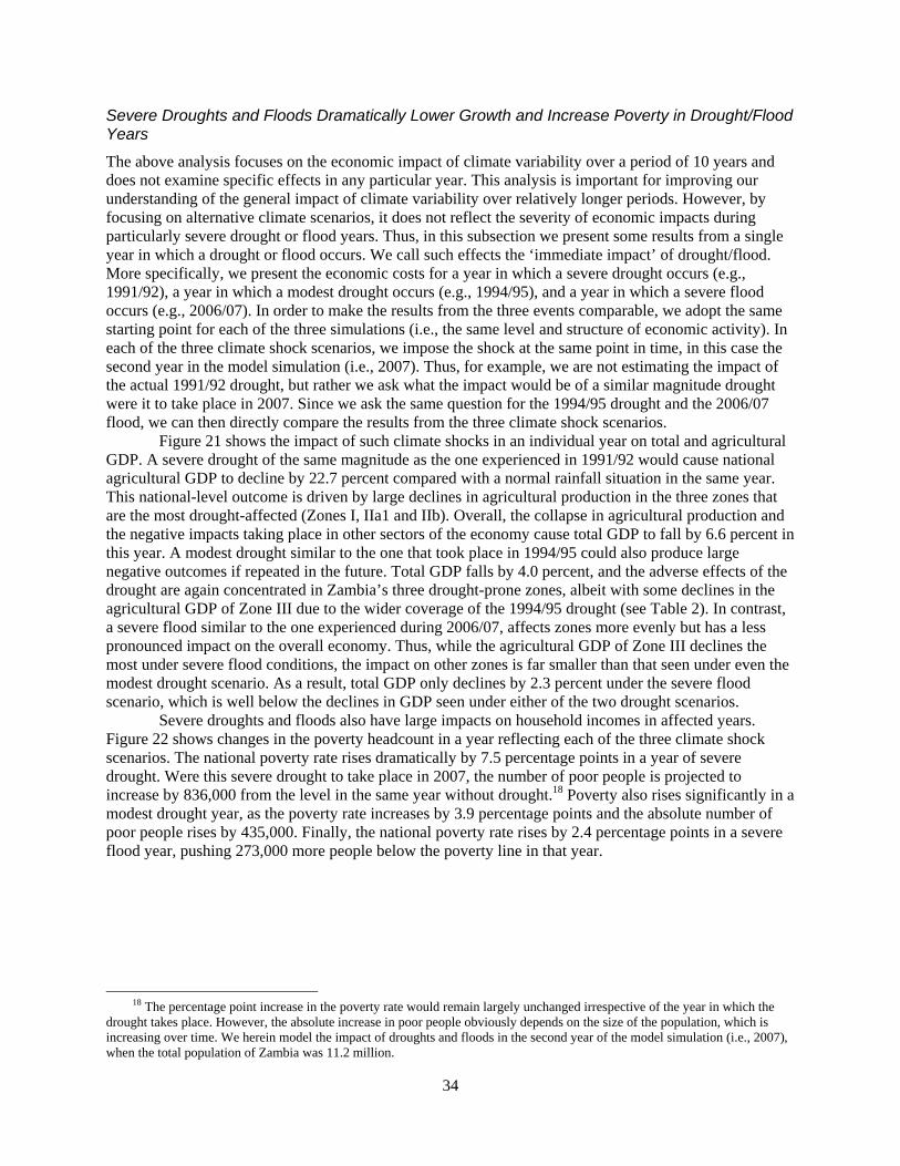
34

Severe Droughts and Floods Dramatically Lower Growth and Increase Poverty in Drought/Flood Years

The above analysis focuses on the economic impact of climate variability over a period of 10 years and does not examine specific effects in any particular year. This analysis is important for improving our understanding of the general impact of climate variability over relatively longer periods. However, by focusing on alternative climate scenarios, it does not reflect the severity of economic impacts during particularly severe drought or flood years. Thus, in this subsection we present some results from a single year in which a drought or flood occurs. We call such effects the ‘immediate impact’ of drought/flood. More specifically, we present the economic costs for a year in which a severe drought occurs (e.g., 1991/92), a year in which a modest drought occurs (e.g., 1994/95), and a year in which a severe flood occurs (e.g., 2006/07). In order to make the results from the three events comparable, we adopt the same starting point for each of the three simulations (i.e., the same level and structure of economic activity). In each of the three climate shock scenarios, we impose the shock at the same point in time, in this case the second year in the model simulation (i.e., 2007). Thus, for example, we are not estimating the impact of the actual 1991/92 drought, but rather we ask what the impact would be of a similar magnitude drought were it to take place in 2007. Since we ask the same question for the 1994/95 drought and the 2006/07 flood, we can then directly compare the results from the three climate shock scenarios.

Figure 21 shows the impact of such climate shocks in an individual year on total and agricultural GDP. A severe drought of the same magnitude as the one experienced in 1991/92 would cause national agricultural GDP to decline by 22.7 percent compared with a normal rainfall situation in the same year. This national-level outcome is driven by large declines in agricultural production in the three zones that are the most drought-affected (Zones I, IIa1 and IIb). Overall, the collapse in agricultural production and the negative impacts taking place in other sectors of the economy cause total GDP to fall by 6.6 percent in this year. A modest drought similar to the one that took place in 1994/95 could also produce large negative outcomes if repeated in the future. Total GDP falls by 4.0 percent, and the adverse effects of the drought are again concentrated in Zambia’s three drought-prone zones, albeit with some declines in the agricultural GDP of Zone III due to the wider coverage of the 1994/95 drought (see Table 2). In contrast, a severe flood similar to the one experienced during 2006/07, affects zones more evenly but has a less pronounced impact on the overall economy. Thus, while the agricultural GDP of Zone III declines the most under severe flood conditions, the impact on other zones is far smaller than that seen under even the modest drought scenario. As a result, total GDP only declines by 2.3 percent under the severe flood scenario, which is well below the declines in GDP seen under either of the two drought scenarios.

Severe droughts and floods also have large impacts on household incomes in affected years. Figure 22 shows changes in the poverty headcount in a year reflecting each of the three climate shock scenarios. The national poverty rate rises dramatically by 7.5 percentage points in a year of severe drought. Were this severe drought to take place in 2007, the number of poor people is projected to increase by 836,000 from the level in the same year without drought.18 Poverty also rises significantly in a modest drought year, as the poverty rate increases by 3.9 percentage points and the absolute number of poor people rises by 435,000. Finally, the national poverty rate rises by 2.4 percentage points in a severe flood year, pushing 273,000 more people below the poverty line in that year.

18 The percentage point increase in the poverty rate would remain largely unchanged irrespective of the year in which the

drought takes place. However, the absolute increase in poor people obviously depends on the size of the population, which is increasing over time. We herein model the impact of droughts and floods in the second year of the model simulation (i.e., 2007), when the total population of Zambia was 11.2 million.

35

Figure 21. Changes in GDP during severe drought and flood years

Note: ‘Severe drought’ reflects the climate conditions in 1991/92, ‘modest drought’ reflects those in 1994/95, and ‘severe flood’ corresponds to 2006/07. Zonal agricultural GDP excludes forestry, but this parameter is included in the national agricultural and total GDP.


Figure 22. Changes in poverty headcount rate during severe drought and flood years

Note: ‘Severe drought’ reflects the climate conditions in 1991/92, ‘modest drought’ reflects those of 1994/95, and ‘severe flood’ corresponds to those of 2006/07. The zonal poverty rates are for farm households only (i.e., 80 percent of the total population), whereas the national poverty rate includes all households.

‐70

‐60

‐50

‐40

‐30

‐20

‐10

0

10

National total GDP

National Zone I Zone IIa1 Zone IIa2 Zone IIb Zone III

Agricultural GDP

Change

in GDP (%)

Severe drought Modest drought Severe flood

‐2

0

2

4

6

8

10

National Zone I Zone IIa1 Zone IIa2 Zone IIb Zone III

Change

in poverty headcount (%

‐point) Severe drought Modest drought Severe flood

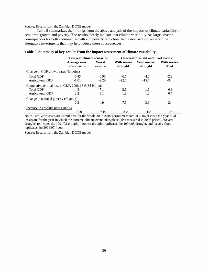
36

Source: Results from the Zambian DCGE model. Table 9 summarizes the findings from the above analysis of the impacts of climate variability on

economic growth and poverty. The results clearly indicate that climate variability has large adverse consequences for both economic growth and poverty reduction. In the next section, we examine alternative investments that may help reduce these consequences.

Table 9. Summary of key results from the impact assessment of climate variability

Ten-year climate scnearios One-year drought and flood events Average over

32 scenarios Worst

scenario With severe

drought With modest

drought With severe

flood

Change in GDP growth rates (%-point)

Total GDP -0.43 -0.90 -6.6 -4.0 -2.3 Agricultural GDP -1.01 -2.29 -22.7 -15.7 -9.4

Cumulative or total loss in GDP, 2006-16 (US$ billion) Total GDP 4.3 7.1 2.6 1.6 0.9 Agricultural GDP 2.2 3.1 1.8 1.2 0.7

Change in national poverty (%-point) 2.2 4.9 7.5 3.9 2.4

Increase in absolute poor (1000s) 300 648 836 435 273

Notes: Ten-year losses are cumulative for the whole 2007-2016 period measured in 2006 prices. One-year total losses are for the year in which the extreme climate event takes place (also measured in 2006 prices). ‘Severe drought’ replicates the 1991/92 drought, ‘modest drought’ replicates the 1994/95 drought, and ‘severe flood’ replicates the 2006/07 flood.


37

5. ADDITIONAL CLIMATE CHANGE IMPACTS ON GROWTH AND POVERTY

Climate Change and Agricultural Crop Yields: Hydro-Crop Model Results

Even with present mitigation measures, the current scientific consensus holds that greenhouse gas emissions and atmospheric concentrations are set to increase for some decades to come. Furthermore, global mean surface temperatures will continue to rise long after emissions have peaked. This global warming is expected to affect global water and food systems in profound ways, as identified by the International Panel on Climate Change (IPCC 2007a). The most serious of these impacts will be mediated via water due to hydrological changes (Rogers 2008). However, in addition to water, two other opposing factors that may also determine the impacts of climate change on agriculture: rising atmospheric CO2 concentrations should increase yields through a process known as ‘carbon fertilization,’ while rising temperatures may substantially reduce yields for some crops. However, among these three factors, changes in the availability of water caused by climate change will have the largest consequences for agriculture (Houghton 2004; Hulme 1996).

Given Zambia’s latitude, temperature increases caused by climate change are likely to reduce crop yields in the country. Conversely, studies have shown that the effects of carbon fertilization should raise crop yields.19 Given the uncertainties surrounding these opposing impacts, especially at the national and per-crop levels, the effects of temperature change and carbon fertilization on crop yields are not examined in this study. Instead, we focus on the yield impacts caused by hydrological changes.

A number of global climate change scenarios have been simulated. Here, we use the SRES B1a scenario of the HadCM3 model, which is a coupled atmosphere-ocean general circulation model developed at the Hadley Centre (henceforth referred to as HadCM3/B1a).20 From this scenario, we obtain mean changes in precipitation, minimum and maximum daily average temperatures, relative humidity, and wind speed for grid cells in Zambia for the next 20 years (until 2025). The HadCM3/B1a scenario is selected because it represents a future climate where rainfall declines and temperatures increase throughout the Zambia, thus potentially jeopardizing agricultural production. We choose the year 2025 because it is the year closest to the 2006-2015 period analyzed in the previous section.21 The changes observed in our analysis are less pronounced than those found in other studies, since 2025 is considerably closer to present day than the more distant projections used elsewhere (e.g., 2050 or 2100). Notably, the IPCC report indicates that alternative global scenarios show little variation until 2030, thus making the use of multiple scenarios less attractive for the purposes of our analysis.

Mean monthly changes in climate variables from the HadCM3/B1a scenario are downscaled to Zambia’s 30 meteorological stations (see Figure 2), and then applied to the historical monthly weather observations for 1976-2007 in order to construct new climate data reflecting climate changes in 2025 as per the SRES B1a scenario. The new climate data are then analyzed using the crop water module described in Section 2, in order to derive yield effects from climate change.

Considerable uncertainty surrounds the effects of climate change, especially at the country level. Accordingly, two climate change scenarios in addition to the HadCM3/B1a scenario are created to examine crop yield responses under larger changes in rainfall and temperature. In the first scenario, we assume that temperatures increase by 2°C in every month throughout the country and rainfall declines by 15 percent from the observed 1975-2007 conditions (this is called the T2P-15 scenario). In the second

19 Recent studies find that carbon fertilization effects may have been overestimated in earlier studies (Long et al., 2006). 20 The data for Zambia come from the IPCC Data Distribution Center (http://www.ipcc‐data.org/). The B1 storyline and

scenario family describe a convergent world in which the global population peaks mid-century and declines thereafter; experiences rapid changes in economic structures toward a service and information economy, with reductions in material intensity; and sees the introduction of clean and resource-efficient technologies. The scenario thus emphasizes global solutions to economic, social, and environmental sustainability (including improved equity), but does not anticipate additional climate initiatives.

21 Economic models become substantially more inaccurate beyond 10-15 years, which recommends 2025 as the maximum range for our analysis.

38

scenario, we also assume that temperatures increase by 2°C, but rainfall now increases by 15 percent from the 1975-2007 series (this is called the T2P+15 scenario). All three of these climate change scenarios represent mean changes in future climate at a fixed-year level from the historical climate. These scenarios do not account for a gradual evolution of climate change. The reason for this simplification is that we use the index sequential method (Prairie et al. 2006) to re-sample the climate series in order to create scenarios to be used in the economic model. This implicitly assumes a stationary climate series and does not allow for gradual changes.

Unlike the HadCM3 scenario, the two additional scenarios are not based on global climate model projections, but rather are used to represent more dramatic changes for Zambia in the intermediate term. They assume uniform changes of temperature and precipitation imposed on the historic temperature and precipitation scenarios derived from all 30 sampled Zambian weather stations for the period 1976-2007. These kinds of hypothetical scenarios are often used in climate change impact assessment and adaptation studies, in order to examine the responses of a study region to a wide range of changes (Zhu et al. 2005; Yates et al. 2007). The 2°C increase in temperature and 15 percent decline of rainfall assumed in the T2P-15 scenario may not necessarily occur by 2025, but the chance that these changes could occur later cannot be underestimated, given that many climate models project a drying trend for Southern Africa and the current level of global greenhouse emission already exceeds the maximum level projected in the IPCC emission scenarios (IPCC 2007a). Likewise, the chance that the warmer and wetter T2P15 scenario could happen in the future cannot be excluded, as certain global climate models project a wetting trend for this region (IPCC 2007a). Indeed, the uncertainties associated with emission scenarios and climate model projections make these hypothetical scenarios useful for examining broader ranges of climate change outcomes.

The climate change scenarios do not explicitly introduce variability changes into the observed meteorological data, but rather cause changes in mean climate. We then analyze the impact of these mean climate changes on crop yields using the hydro-crop model. Table 10 gives the mean and average standard deviation of changes in maize yields relative to the estimated yields for 1976-2007 under each of the three climate change scenarios. Under the HadCM3/B1a scenario, yields decline relative to the estimated historical trend of 1976-2007 for all agroecological zones, with the exception of Zone IIb, in which maize yields increase slightly relative to historical trends. Given that rainfall is generally declining under the HadCM3/B1a scenario, this slight yield increase for Zone IIb is the result of complex interactions of multiple climate variables that jointly determine crop water requirements and soil moisture dynamics. Overall, we conclude that, compared with the past period of 1976-2007, climate change with less rainfall and higher temperature (i.e., the HadCM3/B1a scenario) will result in a 1 percent reduction in maize yields for Zones I, IIa1 and IIa2 by 2025, but no yield change in Zones IIb and III. As the scenario does not capture changes in the patterns of rainfall variation, the standard deviations of maize yields from their historical trends have a similar magnitude to the changes in mean. Although the HadCM3/B1a scenario results in only small changes in maize mean yield relative to historical trends, the impacts in a particular year can be much larger. For example, in a severe drought year similar to that of 1991/92, maize yield is 4 percent lower than it is without climate change effect.

Under the T2P-15 scenario, 4-6 percent declines in maize yields relative to the historical trends are observed in all of the agroecological zones with the exception of Zone III, where the reduction is only 1.4 percent. Again, the magnitude of standard deviations is consistent with the mean change at the zonal level. This implies that there will be an average 4-6 percent drop in maize yields throughout most of Zambia if rainfall declines by 15 percent and temperatures rise by 2 degrees in the future. Under the T2P+15 scenario, the maize mean yield relative to the historical trends increases by 3-4 percent for Zones I, IIa1 and IIb. There is a 2 percent increase for Zone IIa2 and a slight increase for Zone III. In both the T2P-15 and T2P+15 scenarios, the wetter Zone III is fairly resilient to climate changes in terms of crop yield responses to declines or increases in rainfall. In contrast, the four drier zones are likely to face larger changes in crop yields if future rainfall changes and temperatures rise.

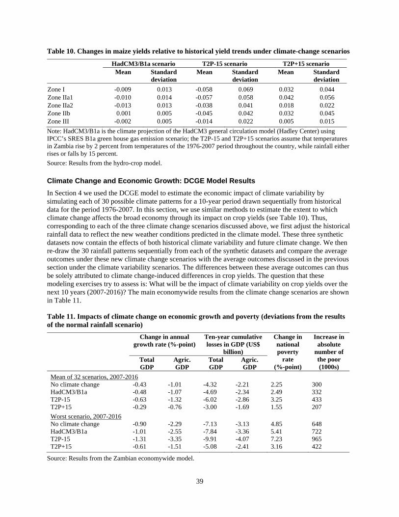
39

Table 10. Changes in maize yields relative to historical yield trends under climate-change scenarios

HadCM3/B1a scenario T2P-15 scenario T2P+15 scenario Mean Standard

deviation Mean Standard

deviation Mean Standard

deviation

Zone I -0.009 0.013 -0.058 0.069 0.032 0.044 Zone IIa1 -0.010 0.014 -0.057 0.058 0.042 0.056 Zone IIa2 -0.013 0.013 -0.038 0.041 0.018 0.022 Zone IIb 0.001 0.005 -0.045 0.042 0.032 0.045 Zone III -0.002 0.005 -0.014 0.022 0.005 0.015

Note: HadCM3/B1a is the climate projection of the HadCM3 general circulation model (Hadley Center) using IPCC’s SRES B1a green house gas emission scenario; the T2P-15 and T2P+15 scenarios assume that temperatures in Zambia rise by 2 percent from temperatures of the 1976-2007 period throughout the country, while rainfall either rises or falls by 15 percent.


Climate Change and Economic Growth: DCGE Model Results

In Section 4 we used the DCGE model to estimate the economic impact of climate variability by simulating each of 30 possible climate patterns for a 10-year period drawn sequentially from historical data for the period 1976-2007. In this section, we use similar methods to estimate the extent to which climate change affects the broad economy through its impact on crop yields (see Table 10). Thus, corresponding to each of the three climate change scenarios discussed above, we first adjust the historical rainfall data to reflect the new weather conditions predicted in the climate model. These three synthetic datasets now contain the effects of both historical climate variability and future climate change. We then re-draw the 30 rainfall patterns sequentially from each of the synthetic datasets and compare the average outcomes under these new climate change scenarios with the average outcomes discussed in the previous section under the climate variability scenarios. The differences between these average outcomes can thus be solely attributed to climate change-induced differences in crop yields. The question that these modeling exercises try to assess is: What will be the impact of climate variability on crop yields over the next 10 years (2007-2016)? The main economywide results from the climate change scenarios are shown in Table 11.

Table 11. Impacts of climate change on economic growth and poverty (deviations from the results of the normal rainfall scenario)

Change in annual growth rate (%-point)

Ten-year cumulative losses in GDP (US$

billion)

Change in national poverty

rate (%-point)

Increase in absolute

number of the poor (1000s)

Total GDP

Agric. GDP

Total GDP

Agric. GDP

Mean of 32 scenarios, 2007-2016 No climate change -0.43 -1.01 -4.32 -2.21 2.25 300 HadCM3/B1a -0.48 -1.07 -4.69 -2.34 2.49 332 T2P-15 -0.63 -1.32 -6.02 -2.86 3.25 433 T2P+15 -0.29 -0.76 -3.00 -1.69 1.55 207

Worst scenario, 2007-2016 No climate change -0.90 -2.29 -7.13 -3.13 4.85 648 HadCM3/B1a -1.01 -2.55 -7.84 -3.36 5.41 722 T2P-15 -1.31 -3.35 -9.91 -4.07 7.23 965 T2P+15 -0.61 -1.51 -5.08 -2.41 3.16 422


40

The top half of Table 11 shows deviations in the mean of all rainfall scenarios from the results

under the normal rainfall scenario. As discussed in Section 4, if climate variability follows its historical patterns without accounting for possible climate change, the average decline in the annual growth rate of total GDP is 0.4 percentage points. The first row of Table 11 repeats the results from Figure 15 in Section 4. Incorporating the effects of climate change produces mixed results. The loss in total GDP growth is slightly larger under the HadCM3/B1a scenario, but it becomes substantially larger under the T2P-15 scenario, which captures potential declines in average rainfall due to climate change. Moreover, the higher average rainfall under the T2P+15 scenario dampens the adverse effects of climate variability on growth, with the result that the average decline in GDP growth is smaller than that seen in the case without climate change (Table 11). These results indicate that if climate changes cause less rainfall every year, the economic annual growth rate would decline further by between 0.05 percentage points (under the HadCM3/B1a scenario) and 0.20 percentage points (under the T2P-15 scenario) in each of the next 10 years. However, if climate changes cause more rainfall (as under the T2p+15 scenario), the GDP growth rate would be slightly higher than that seen without climate change (by 0.14 percentage points). The implications of these seemingly small changes in the total GDP growth rate become more substantial once their effects are accumulated over the 10-year simulation period (i.e., 2007-2016). For instance, the cumulative declines in total GDP under the T2P-15 scenario are US$6 billion (in 2006 prices; US$1.7 billion more than seen without climate change effects) compared to US$3 billion under the T2P+15 scenario (US$1.3 billion less than seen without climate change effects). Even under the modest HadCM3/B1a scenario, climate change increases the costs already accrued due to climate variability by an additional US$0.37 billion over the 10-year period (US$4.69 billion in total in 2006 prices; see Table 11). Thus, while the economic implications of climate change may appear inconsequential at any given point in time, their gradual impact on both total and agricultural GDP becomes more significant over time.

The second part of Table 11 presents deviations in outcomes from the worst rainfall scenario reported in Section 4. If Zambia’s rainfall patterns over the next 10 years replicate those observed during the 1984/85 to 1994/95 period, then the total growth rate will be 0.9 percentage points lower than it would have been under a normal rainfall scenario without variability (see Section 4). However, when we incorporate the impact of climate change derived from the HadCM3/B1a scenario, the drop in GDP growth rate rises to 1.01 percentage points (i.e., a further 0.1 percentage point decline). Over 10 years, this reduced GDP growth rate results in an accumulated GDP loss of US$0.7 billion (in 2006 prices). Under the more pessimistic T2P-15 scenario, additional cumulative losses rise dramatically to US$9.9 billion, which is almost US$3 billion more than that observed when we do not account for climate change effects. Conversely, if the more optimistic T2P+15 scenario is accurate, then we see a smaller GDP loss, and the accumulated losses fall to US$5.08 billion, which is US$2 billion less than that seen for scenarios without climate change effects and those including climate variability alone.

Finally, the impacts of climate change on national poverty rates and the absolute number of poor people by 2016 are reported in the last two columns of Table 11. Since climate change further increases the effects of climate variability on agricultural production and food prices, there are significant differences in poverty outcomes across the three climate change scenarios. For instance, even with the modest HadCM3/B1a scenario, the national poverty rate projected for 2016 is 0.24 percentage points higher than that obtained in the absence of climate change (i.e., the poverty rate increases by 2.5 percent instead of 2.3 percent by 2016). Thus, climate change increases the absolute number of poor people in 2016 by 32,000. Similarly, under the worst rainfall scenario together with the HadCM3/B1a scenario, the poverty rate is projected to be 0.6 percentage points higher as a result of climate change. These deviations in poverty rates are substantially larger for the two hypothetical climate scenarios (i.e., less rainfall increases poverty while more rainfall lowers poverty).

Overall, in Zambia, the additional impact of future climate change on economic growth and poverty is substantially smaller than that of climate variability (based on historical patterns). Even under more pessimistic climate change scenarios, the effects of climate change are less than half those projected

41

for the climate variability scenarios. However, it should be noted that the climate change scenarios in this study do not capture possible changes in climate variability and hence provide only partially illustrative results for potential climate change impacts in Zambia. We find that the expected changes remain fairly small under the HadCM3/B1a scenario. However, the impacts can be more pronounced if larger changes in rainfall and temperature occur (as illustrated by the two hypothetical climate change scenarios) or if climate variability patterns change. Moreover, while the average change over the longer term is relatively small, considerable impacts may be seen in specific years, especially if there is even less rainfall than that experienced during the severe drought years observed in Zambia’s history. Moreover, because we do not explicitly capture any possible changes in the patterns of climate variability caused by climate change, worsening climate variability exacerbated by climate change may have unexpected subnational impacts on the Zambian economy. This possibility emphasizes the importance of investing in climate mitigation efforts and strategies aimed at reducing Zambia’s vulnerability to extreme rainfall events.

42

6. SUMMARY AND CONCLUSIONS

Zambia’s economic performance over the past three decades has been hampered by high levels of climate variability and frequent and severe droughts and floods. Even in more recent years, when the country’s economy has performed better, there has still been considerable variation in the growth rate of the agricultural sector. In order to assess the consequences or impacts of climate variability on economic growth and poverty reduction in Zambia, we herein develop an integrated analytical framework. First, we use historical climate data and a hydro-crop model to estimate the impact of climate variability on crop yields over the past three decades. This analysis is done at the crop level for each of Zambia’s five agroecological zones, supported by the identification of zonal-level extreme weather events using a drought index analysis. Drawing on these results, we then develop an economywide CGE model and analyze the impact of climate variability-induced changes in crop yields on economic growth and poverty. In doing this, we consider not only the main impact channel of yield declines, but also other indirect impact channels, including effects on crop areas, livestock stocks, and depreciation of physical capital.

The findings from our economywide modeling assessment suggest that climate variability has a pronounced negative effect on economic growth. We estimate that, on average, climate variability reduces Zambia’s GDP growth rate by 0.4 percentage points per year, which costs the country US$4.3 billion over a 10-year period. These losses reach as high as US$7.1 billion under Zambia’s worst rainfall scenario. Agriculture is especially vulnerable and forms the primary impact channel, with climate variability reducing agriculture’s annual GDP growth rate by at least 1 percentage point, and by over 2 percentage points during the worst rainfall scenario. This will greatly reduce Zambia’s chances of achieving the national development goal of strengthening agricultural and rural income growth. Indeed, we find that the negative effect of climate variability is especially severe for maize, the country’s main food staple crop, and that it therefore greatly threatens basic food security in both rural and urban areas. Most of the negative impacts of climate variability occur in the southern and central regions of the country, where food insecurity is most vulnerable to climate shocks. Overall, climate variability keeps 300,000 people below the national poverty line by 2016. While most of these people live in rural areas, climate variability also greatly increases urban poverty due to higher food prices and lower real urban incomes. The number of poor rises substantially if rainfall patterns are similar to those experienced in 1985-1995, when the country experienced a series of severe droughts. Indeed, the national poverty rate may rise by as much as 8 percentage points in particularly severe drought years. Climate variability has thus played a significant role in undermining economic development in Zambia in the past and will continue to do so in the future.

We also examine whether climate change will exacerbate or dampen the negative consequences of climate variability. Here considerable uncertainty exists, especially regarding changes in future rainfall patterns. Accordingly, while we used a well-known climate change projection model, we also analyze two hypothetical scenarios. We find that the effects of current patterns of climate variability dominate over those of potential climate change in the near future (until 2025). However, differences in assumptions regarding rainfall changes influence both the size (to a large degree) and direction (to a lesser extent) of the economic impact of climate change. If rainfall declines by 15 percent, then climate change enhances the negative effects of climate variability by a factor of 1.5 and pushes an additional 30,000 people below the poverty line over a 10-year period. Moreover, the effects of climate change and variability compound each other, with the number of poor people rising to 74,000 if climate change is coupled with Zambia’s worst 10-year historical rainfall pattern. Thus, climate change may further exacerbate the negative consequences of climate variability. There is considerable scope and incentive, therefore, to invest in irrigation and water management practices aimed at mitigating the adverse effects of both climate variability and climate change on Zambia’s economic development.

43

APPENDICES

Appendix A: Description of the Hydro-Crop (HC) Model

Quantitative information on crop yield responses to water deficiency is crucial for evaluating the economic impacts of climate variability and change on agricultural production. Here, we develop a semi-empirical model that includes two modules. The first module simulates the soil water balance in the crop root zone to derive actual evapotranspiration (ET). The second module estimates crop yield responses to water deficits using an empirical crop water production function that takes into account growing stage-specific crop sensitivity to water stress. Together, these two modules form the integrated ‘hydro-crop’ model used in this study.

The soil water balance module regards the crop root zone as a bucket with water flowing in through rainfall (and irrigation if applicable) and leaking away as ET, runoff and deep percolation. The first step in determining the soil water balance is to estimate crop water requirements, which are normally expressed as a rate of potential ET. The potential ET for a particular crop is estimated using the potential ET of a reference crop, usually alfalfa, and a calibrated crop coefficient that converts the reference ET to the crop’s potential ET under given climatic conditions. With rainfall and potential ET, the soil water balance module calculates the actual ET and water surplus using the actual soil water content and the available water capacity (AWC) in the crop root zone. If the soil water content is above a threshold level of AWC, then actual ET takes place at the potential rate. It is not, then actual ET is constrained by soil moisture. Surface runoff and deep percolation occur if the estimated end-of-period soil water content exceeds the AWC. The soil water balance module runs continuously and produces actual ET, which is then used in the crop water production function to estimate the crop yield reduction resulting from a water deficit. As daily climate data are not available, the soil water balance simulations are done for monthly intervals using long-term monthly data.

The second module in the hydro-crop model is a nonlinear Jensen crop water production model. It is used to estimate crop yield responses to water using monthly data for actual and potential ET values during the crop-growing season. The Jensen function is an empirical water production function. It has an advantage over the FAO crop yield response model in that the Jensen function can account for the crop’s growth stage-specific sensitivity to water, whereas the FAO model only considers water deficits for the entire growing season and thus cannot capture monthly climate variations and crop yield sensitivities to water. We compared observed yields across the five agroecological zones in Zambia with simulations from both Jensen and FAO models and found that the Jensen function outperformed the FAO model for our purposes. This is in part because crop losses in Zambia are particularly sensitive to seasonal water deficits, especially in major drought years. For each crop, the water sensitivity index values in the Jensen crop water production function are estimated based on stage-specific FAO yield response factors using OLS regression. These are then mapped to each month in the crop’s growing period, using a cumulative sensitivity index method.

For all crops and all agroecological zones in Zambia, hydro-crop model simulations are done based on observed meteorological data provided by the Zambia Department of Meteorology. Here, we use monthly climate data obtained from 1975 to 2007 at 30 meteorological stations. Rainfall and calculated potential ET are aggregated to the five agroecological zones based on the estimated influencing domain of each station. The latter are based on the area of each Thiessen polygon within a zone and the areas of other Thiessen polygons within the same agroecological zone.

44

Appendix B

Table B1. Specification of the Hydrological and Crop Production Models

Model Parameter Unit

Crop Water Requirement

Kc Crop coefficient - γ Psychrometric constant kPa °C-1

KRs Radiation adjustment coefficient -

Soil Water Balance Smax Maximum tension water capacity in root zone mm m-1

f Field capacity mm m-1

w Wilting point mm m-1

rZ Root zone depth m

p Fraction of active tension water capacity in root zone below which crop begins to experience stress

-

Crop Water Production Function

Ymax Maximum yield without water stress t ha-1 Ky Yield response factor -

λt Crop water sensitivity index -

Model Variable Unit


ETo Reference evapotranspiration mm PET Crop potential evapotranspiration mm

Rs Incoming solar radiation MJ m-2 day-1

Rn Net radiation at the crop surface MJ m-2 day-1

Ra Extraterrestrial radiation MJ m-2 day-1

G Soil heat flux density MJ m-2 day-1

T Mean daily air temperature at 2 m height °C

Tmax Maximum daily air temperature at 2 m height °C

Tmin Minimum daily air temperature at 2 m height °C

es Saturation vapor pressure kPa

Δ Slope vapor pressure curve kPa °C-1

u2 Wind speed at 2 m height m s-1

Soil Water Balance P Rainfall mm AET*

Predicted actual crop evapotranspiration mm

AET Adjusted actual crop evapotranspiration mm

S Soil water content in root zone mm

Crop Water Production Function

Ya Actual crop yield t ha-1

45

Table B1. (Continued) Model Equation Equation No. Notes


2

2

34.01273

900408.0

u

eeuT

GRET

asn

o

2.1 FAO Penman-Monteith equation (Allen et al. 1998) for calculating reference evapotranspiration

aRss RTTKR 5.0minmax

2.2 Hargreaves’ radiation formula as recommended by Allen et al. (1998) when radiation data are not available

oct ETKPET

2.3 Crop potential evapotranspiration (Allen et al. 1998)

Soil Water Balance rwf ZS )(max

2.4 Active tension water

capacity in root zone

max1

max1max

1*

，

,

SpPSPET

SpPSPETSp

PS

AET

ttt

ttttt

t

2.5 Predicted actual crop evapotranspiration

tttt PSAETAET 1

* ,min

2.6 Adjusted crop actual evapotranspiration

max1max

max11

,

,

SAETPSS

SAETPSAETPSS

tt

ttttt

t

2.7 End of period soil water content

Crop Water Production Function Tt

PET

AETKYY

tt

tt

ya

,11max

2.8 FAO yield response function (Doorenbos and Kassam 1979)

Tt t

ta

t

PET

AETYY

max

2.9 Jensen crop water production function (Jensen 1968)

46

Appendix C: Description of the Economywide Model and the Zambian Economy

A dynamic computable general equilibrium (DCGE) model of Zambia is herein developed to examine the economywide growth and poverty impacts of the climate variability predicted by the hydrological model. In order to better understand how the output of the hydrological model becomes the input of a DCGE model and how climate variability directly and indirectly affects the economy, we provide a brief description of the DCGE model and its use in the present study. In general, a CGE model is a multi-sector general equilibrium model; the model developed for this study also contains detailed information on subnational production and employment, as well as national levels of domestic and international trade. Households and their income sources are also considered at the subnational level, which allows the model to be used for welfare and poverty analysis at the national and subnational levels according to the different types of household groups. Below, we discuss the structure of the model in detail with reference to the Zambian economy. We then describe how the DCGE model incorporates the output of the hydrological model for use in this study.

Production and Employment

The DCGE model of Zambia contains 34 production sectors that produce 34 commodities. Among the 34 sectors, 17 belong to the agricultural sector, nine are industrial and eight are service sectors (see Table C1 for the list of sectors). Agricultural crops fall into four broad groups: (i) cereals, including maize, sorghum, millet, and other cereals (i.e., wheat and rice); (ii) root crops, such as cassava, Irish potatoes, and sweet potatoes; (iii) other food crops, including pulses, groundnuts, other oilseeds, vegetables, and fruits; and (iv) higher-value export-oriented crops, including cotton, sugar, tobacco, and other export crops (e.g., soybeans). The CGE model also identifies three livestock subsectors, namely cattle, poultry, and other livestock (e.g., sheep, goats and pigs). The two remaining agricultural subsectors are forestry and fisheries. Together, these agricultural subsectors account for 22 percent of gross domestic product (GDP) and 16 percent of exports (see Table C2).

47

Table C1: Sectors in the DCGE model

Agricultural subsectors Irrigated Regional disaggregation

Cereals

1 Maize No 5 Zones, urban & large-scale

2 Sorghum & millet No 5 Zones, urban & large-scale

3 Other cereals (i.e., wheat and rice) Yes 5 Zones, urban & large-scale

4 Root crops (incl. cassava, sweet and Irish potatoes) No 5 Zones, urban & large-scale

Other food crops

5 Pulses & oils (incl. beans) No 5 Zones, urban & large-scale

6 Groundnuts No 5 Zones, urban & large-scale

7 Vegetables No 5 Zones, urban & large-scale

8 Fruits No 5 Zones, urban & large-scale

High-value export-oriented crops

9 Cotton No 5 Zones, urban & large-scale

10 Sugarcane Yes 5 Zones, urban & large-scale

11 Tobacco No 5 Zones, urban & large-scale

12 Other crops (mainly soybeans) Yes 5 Zones, urban & large-scale

Livestock

13 Cattle 5 Zones & urban

14 Poultry 5 Zones & urban

15 Other livestock (incl. goats, sheep and pigs) 5 Zones & urban

16 Fisheries 5 Zones

17 Forestry National

Industrial subsectors

18 Mining National

19 Food processing, beverages & tobacco National

20 Textiles & clothing National

21 Wood & paper products National

22 Chemicals & rubber products National

23 Machinery & equipment (incl. vehicles) National

24 Other manufacturing (incl. furniture) National

25 Electricity & water National

26 Construction National

Service subsectors

27 Trade services National

28 Hotels & catering National

29 Transport & communication services National

30 Financial, business & real estate services National

31 Government administration National

32 Education services National

33 Health services National

34 Community & other services National

Source: 2006 SAM of Zambia.

48

Table C2: National production and trade structure of the Zambian economy

Share of total (%) Trade intensity GDP Exports Imports Exports Imports

Total GDP 100.00 100.00 100.00 19.85 21.67

Agriculture 21.94 15.75 5.65 15.54 6.63 Cereals 9.48 4.06 4.13 9.13 9.78

Maize 8.78 3.91 2.28 9.42 6.04 Sorghum & millet 0.43 0.08 5.20 Other cereals 0.27 0.15 1.77 11.01 60.85

Root crops 0.67 0.56 0.11 24.08 6.24 Other food crops 4.33 0.02 0.65 0.12 3.93

Pulses & oils 0.40 0.02 0.14 1.27 8.82 Groundnuts 1.53 Vegetables 1.73 Fruits 0.68 0.50 18.40

Export-oriented crops 3.46 9.67 0.33 64.60 6.43 Cotton 1.14 4.90 0.13 84.61 13.46 Sugarcane 1.61 2.46 42.03 Tobacco 0.46 1.20 54.01 Other crops 0.25 1.12 0.20 100.00 100.00

Livestock 2.26 0.17 0.20 1.29 1.78 Cattle 0.88 0.19 4.94 Poultry 0.71 0.00 0.07 Other livestock 0.68 0.17 0.01 5.47 0.38

Fisheries 0.93 0.94 21.60 Forestry 0.80 0.32 0.23 7.40 6.05

Mining 7.10 69.06 98.89

Manufacturing 11.97 5.01 69.25 5.86 49.55 Food processing 6.46 1.86 3.15 4.57 8.44 Textiles & clothing 1.75 5.93 36.99 Wood & paper products 1.14 2.05 1.65 24.13 22.06 Chemicals & rubber products 1.08 1.11 23.51 8.79 69.01 Machinery & equipment 1.26 33.04 79.78 Other manufacturing 0.28 1.97 55.29

Electricity & water 2.95

Construction 5.73

Services 50.31 10.18 25.09 5.09 12.29 Trade services 17.36 Hotels & catering 2.94 5.98 47.86 Transport & communication 4.78 4.20 21.52 19.59 56.97 Financial and business services 4.65 3.57 17.55 Government administration 8.07 Education services 8.90 Health services 2.97 Community & other services 0.63

Note: Export intensity is the share of exports in domestic output, and import intensity is the share of imports in domestic supply.

Source: 2006 SAM of Zambia.

49

Zambia’s industrial sectors account for 28 percent of GDP, meaning that together they are similar in size to the agricultural sector. However, most of the manufacturing sectors (e.g., food processing, textiles and wood products) are linked to agriculture; most agricultural commodities are not only exported or consumed by households in Zambia, but are also used as inputs for upstream processing activities, which together generate an additional 9 percent of GDP. However, while agriculture and related sectors dominate GDP, copper is the most important export, generating 70 percent of total export earnings. Almost all mining production is exported, reflecting the relatively weak linkages between this sector and the rest of the economy. The DCGE model captures Zambia’s sectoral structure and its intersectoral linkages by drawing on the information contained in the 2006 social accounting matrix (SAM).22

Beyond its sectoral detail, the DCGE model also captures subnational or spatial heterogeneity in production patterns. Based on district-level data from the 2004/05 Crop Forecasting Survey (CFS04/05), agricultural production is disaggregated across the five agro-climatic regions in a manner similar to that seen in the hydrological model [i.e., Zambia’s four agroecological zones, with Zone IIa further divided into western (Zone IIa1) and eastern (Zone IIa2) sub-zones]. Moreover, we capture the unique circumstances of urban agriculture by separately identifying agricultural production for the main urban centers based on household production information drawn from the 2004/05 Living Standards Monitoring Survey (LCMS4).23 Thus, six subnational regions are identified in the model: five rural and one urban. Finally, a seventh group comprising large-scale farmers is separated from the small/medium-scale producers that tend to be zone-specific. The different cropping patterns of these farm groups are shown in Table C3.

Forty-two percent of harvested land is allocated to maize production, making maize the main crop in Zambia. Scale of production is therefore a key distinguishing feature among farmers. While large-scale farmers represent only 8 percent of total maize land, they produce 22 percent of maize in the country.24 There is virtually no irrigated maize production in Zambia. Average yields for large-scale farmers are high for dry-land production at over 6 tons per hectare in 2005, a year with relatively good rainfall. In contrast, small-scale farmers, who account for four-fifths of maize production, achieve much lower yields of around 2 tons per hectare. The agroecological conditions across zones are also important factors in determining the yield level. Smallholder maize yields range from around 1.5 tons per hectare in the southern and western regions (Zones I and IIb) to 2.4 tons per hectare in the central region (Zone IIa1). Other factors also serve to concentrate maize production within specific regions. For instance, four-fifths of large-scale maize production takes place in Zone IIa1, where the agroecological conditions are more favorable in a normal rainfall year and farmers have better access to urban centers. Finally, urban-based farmers are also an important part of Zambia’s agricultural system. Around a quarter of urban households engage in agricultural production, primarily maize cropping and livestock. Thus, in summary, while Zone III is the largest region in terms of cultivated land size, the central Zone IIa1 dominates maize production in Zambia due to higher maize yields and a concentration of large-scale and urban farmers in this region.

The remaining cereal groups differ sharply in their production structures and technologies. On one hand, sorghum and millet is overwhelmingly a smallholder crop and is particularly important as a drought-tolerant staple in Zambia’s drier southern region (Zone I). On the other hand, wheat (which is aggregated into the ‘other cereals’ subsector in the model) is grown entirely under irrigation, by large-scale farmers in the southern and central regions of the country (Zones I and IIa1). Some smallholders grow rice (also included in ‘other cereals’), especially in the northern region, but relatively little land is allocated to this crop. As such, the ‘other cereals’ group is treated as being entirely irrigated. Finally, as with maize, the regional concentration of wheat production reflects differences in agroecological conditions and market access, and further justifies the division of Zone IIa into eastern and western sub-zones in our study.

22 The 2006 Zambia SAM is an updated and aggregated version of the 2004 SAM used in Thurlow et al. (2008). 23 Metropolitan centers are defined as urban areas in the districts of Kabwe (Central); Chingola, Chililabombwe, Kitwe,

Kalulushi, Lufwanyama, Mufulira and Ndola (Copperbelt); Lusaka (Lusaka); and Livingstone (Southern). 24 Large-scale farmers in Zambia are defined as those having more than 20 hectares of land.

50

Table C3: National production and trade structure of the Zambian economy

Share of total (%) Trade intensity GDP Exports Imports Exports Imports

Total GDP 100.00 100.00 100.00 19.85 21.67

Agriculture 21.94 15.75 5.65 15.54 6.63 Cereals 9.48 4.06 4.13 9.13 9.78

Maize 8.78 3.91 2.28 9.42 6.04 Sorghum & millet 0.43 0.08 5.20 Other cereals 0.27 0.15 1.77 11.01 60.85

Root crops 0.67 0.56 0.11 24.08 6.24 Other food crops 4.33 0.02 0.65 0.12 3.93

Pulses & oils 0.40 0.02 0.14 1.27 8.82 Groundnuts 1.53 Vegetables 1.73 Fruits 0.68 0.50 18.40

Export-oriented crops 3.46 9.67 0.33 64.60 6.43 Cotton 1.14 4.90 0.13 84.61 13.46 Sugarcane 1.61 2.46 42.03 Tobacco 0.46 1.20 54.01 Other crops 0.25 1.12 0.20 100.00 100.00

Livestock 2.26 0.17 0.20 1.29 1.78 Cattle 0.88 0.19 4.94 Poultry 0.71 0.00 0.07 Other livestock 0.68 0.17 0.01 5.47 0.38

Fisheries 0.93 0.94 21.60 Forestry 0.80 0.32 0.23 7.40 6.05

Mining 7.10 69.06 98.89

Manufacturing 11.97 5.01 69.25 5.86 49.55 Food processing 6.46 1.86 3.15 4.57 8.44 Textiles & clothing 1.75 5.93 36.99 Wood & paper products 1.14 2.05 1.65 24.13 22.06 Chemicals & rubber products 1.08 1.11 23.51 8.79 69.01 Machinery & equipment 1.26 33.04 79.78 Other manufacturing 0.28 1.97 55.29

Electricity & water 2.95

Construction 5.73

Services 50.31 10.18 25.09 5.09 12.29 Trade services 17.36 Hotels & catering 2.94 5.98 47.86 Transport & communication 4.78 4.20 21.52 19.59 56.97 Financial and business services 4.65 3.57 17.55 Government administration 8.07 Education services 8.90 Health services 2.97 Community & other services 0.63

Note: Export intensity is the share of exports in domestic output, and import intensity is the share of imports in domestic supply. Source: 2006 SAM of Zambia.

51

The remaining food crops are distributed across the country roughly in proportion to each zone’s total land area. The only exception is root crops. Although cassava and potatoes are grown in all zones, they are particularly important in the eastern and northern regions (Zones IIa2 and III), where a larger amount of land is allocated to root crops than to maize. Finally, Zambia’s export crops are also concentrated in some specific zones. Cotton is grown in the eastern and central regions (Zone IIa) under smallholder out-grower schemes, while tobacco is almost exclusively grown in the eastern region (Zone IIa2) by both small- and large-scale farmers. Both of these crops are grown on dry lands. In contrast, sugarcane and soybeans (included in ‘other crops’ subsector in the model) are grown under irrigation by large-scale farmers in the center of the country (i.e., Zone IIa2). Finally, livestock is an important agricultural subsector, generating 10 percent of agricultural GDP. Three quarters of livestock GDP is found in Zones I and IIa1, where cattle herds and poultry stocks are largest and form an important source of rural incomes.

The DCGE model captures differences in production technologies, such as the higher labor-intensity of agriculture and the capital-intensity of industry. Here the model identifies eight factors of production: three types of labor (unskilled workers, skilled workers, and family farm labor); three kinds of capital (agricultural, mining and nonagricultural); and two kinds of agricultural assets (land and livestock stocks). Skilled and unskilled workers are assumed to be fully employed and are able to migrate across regions and sectors in response to changes in labor demand. However, family farm labor and agricultural capital can only be allocated across farm activities within each zone. Since we are interested in capturing the impact of rainfall variation shocks, we assume that the allocation of land, livestock stocks, and nonagricultural capital across different production activities is constant, so these factors are immobile across sectors and earn sector-specific returns. Producers in each zone and sector employ the eight different factors at varying intensities in order to maximize profits under constant returns to scale, with the choice between factors governed by a constant elasticity of substitution (CES) function. Composite factors are then combined with intermediate inputs under a Leontief specification with fixed input-output coefficients taken from the input-output table underlying the 2005 Zambian SAM.

Domestic and International Trade

Table C2 shows the structure of foreign trade in Zambia, and clearly reveals that the country is heavily dependent on mining exports. However, there was considerable growth in agricultural exports during the 1990s, especially in cotton and sugarcane. Zambia is both an importer and exporter of maize, with the net trade position varying from year to year and depending on the rainfall situation. Most large-scale wheat production in the country is for the domestic market, and some wheat imports are needed, although at relatively low levels. Imports are actually dominated by nonagricultural products. Chemicals (including fuels) and machinery (including vehicles and equipment) are highly import-intensive subsectors. Thus, despite being landlocked, Zambia is heavily reliant on international trade, which in turn is concentrated within a narrow range of commodities for both exports and imports.

The DCGE model captures these linkages with the rest of the world through exports and imports. Producers in each region supply their output to a national commodity market, where they are exported, sold domestically, and/or combined with imported goods. Substitution possibilities exist between production for domestic and foreign markets based on a constant elasticity of transformation (CET) function. Profit maximization drives producers to sell in those markets where they can achieve the highest returns. These returns are based on domestic and export prices (where the latter is determined by the world price times the exchange rate). Substitution possibilities also exist between imported and domestic goods under a CES Armington specification. The ratio of imports to domestic goods is determined by the cost-minimizing decision-making of domestic demanders based on the relative prices of imports and domestic goods (both of which include the relevant taxes).

Under the small-country assumption, Zambia faces perfectly elastic foreign demand/supply from the world at fixed world prices. However, with imperfect substitution between domestically produced and consumed goods and export or import goods, prices for all commodities either produced or sold in

52

domestic markets are endogenous. While an integrated domestic market is assumed, agricultural products produced from different zones are imperfectly substitutable.

Household Incomes and Poverty

The DCGE model distinguishes among various representative household groups. While representative households are zone-specific, they are further disaggregated into rural and urban areas. Rural households within each zone are further distinguished into three groups: small farm, large-scale farm, and non-farm households. Urban and metropolitan households are disaggregated into two groups depending on whether or not they engage in agricultural production. Each of the 27 representative households in the DCGE model is an aggregation of individual households captured in the 2004/05 household survey (LCMS4). Households in the model receive income from different factors employed in different production processes. They then pay taxes to and/or receive transfers from the government. A part of household incomes come from abroad as remittance receipts. As the dynamics of the model are recursive, fixed saving rates are assumed for each representative household. The income allocated to consumption of different commodities is derived from maximizing a Stone-Geary utility function, which results in a linear expenditure system (LES) of demand.25

Table C4 provides income and poverty statistics for the representative aggregate household groups used in the model. Poverty is extremely high in Zambia, with 67.9 percent of the population of 11 million falling below the official poverty line of around US$300 per person per year. Poverty is highest in rural areas, where 61 percent of the population resides. As a result, more than 70 percent of Zambia’s poor population lives in rural areas where, on average, they derive about 80 percent of their incomes from agriculture.

Poverty rates are high in all five of the rural zones identified in the DCGE model. However, there is some variation, with poverty lowest in Zone IIa2 and highest in Zone IIb. The former includes many cotton farmers, whose rising incomes were instrumental in reducing rural poverty in Zambia during the mid-1990s. However, while per capita incomes are highest in Zone IIa1, poverty rates in this zone are still high at 79 percent. This reflects Zambia’s high income inequality, with the relatively few households located closest to large urban centers and major transport routes having a considerably lower incidence of poverty.26 Finally, Table C4 shows average farm plot sizes for the different household groups, which vary greatly across zones. Farm plots are smallest in urban areas and in Zone IIb and largest in the more sparsely populated Zone IIa2. The DCGE model captures these differences in household income patterns, as well as differences in income spending. To assess the impact of the alternative rainfall scenarios on household poverty, the DCGE model needs to link with a micro-simulation model that includes each sample household in the 2004/05 LCMS. These sample households are further linked to their corresponding representative household in the DCGE model on the consumption side. In this formulation, changes in representative households’ consumptions of individual commodities (resulting from income and commodity price changes) in the DCGE model are passed down to their corresponding households in the micro-simulation model, where total consumption expenditures are recalculated in real terms. This new level of per capita expenditure for each survey household is compared to the official poverty line, and standard poverty measures are recalculated.

Model Closure and Dynamics

The DCGE model captures the workings of the government, which receives revenues from imposing activity, sales and direct taxes and import tariffs, and then makes transfers to households and the rest of the world. The government also purchases commodities in the form of government consumption or recurrent expenditures, and the remaining income of government is (dis)saved. All savings from

25 The LES specification identifies a portion of consumption for subsistence (it is income and price independent). The remaining consumption quantities are sensitive to price and income changes. Commodity income elasticities are taken from Thurlow et al. (forthcoming) and allow for differences between marginal and average budget shares.

26 See Thurlow and Wobst (2006) on the role of remoteness in determining rural poverty in Zambia.

53

households, government and capital inflows from abroad (foreign savings) form a savings pool from which investment is financed.

The model contains three macroeconomic accounts: (i) the government account; (ii) the savings-investment account; and (iii) the current account. To balance among the macroeconomic accounts, it is necessary to specify a set of ‘macroclosure’ rules that provide a mechanism through which macroeconomic balance can be achieved. Following Solow’s growth theory, a savings-driven closure is assumed in order to balance the savings-investment account. Under this closure, households’ savings rates are held fixed, and investment adjusts endogenously to equalize investment and savings in equilibrium. In the government account, the direct tax rates on households and capital are assumed to remain unchanged, with government revenues and expenditures balancing through changes in public spending and the fiscal deficit. Finally, for the current account we assume that foreign savings (i.e., foreign capital inflows) are constant. The exchange rate is chosen as the model’s numéraire.

Our DCGE model is a ‘recursive’ dynamic model, which means that there is no intertemporal decision-making for households, either as consumers or as producers. Thus, the stock variables must be updated between periods. While growth in the population (and hence in the labor supply and agricultural land expansion) is exogenously determined between periods, the capital accumulation is endogenously constrained by the level of investment in previous time periods. Once the new capital is formed from the previous periods’ investments, it becomes part of the capital stock that is allocated to different sectors according to the sectoral level of capital returns. This implies that sectors with above-average returns in the previous period receive a larger share of the new capital stock in the current period.

54

Table C4: Household income and poverty characteristics

Population (1000)

Households (1000)

Per capita expenditure

Poverty rate (%)

Average size and allocation of crop land (ha)

Total Poor Total Size Kw 1000 $US All crops Maize Roots Other foods Export crops

All households 10,986 7,461 2,089 5.26 1,861 417 67.9 - - - - -

Urban households 4,298 2,271 814 5.28 3,242 726 52.8 - - - - -

Non-farm 3,075 1,484 619 4.97 3,625 812 48.3 - - - -

Farm 1,223 793 195 6.26 2,281 511 64.8 0.25 0.17 0.00 0.08 0.00

Rural households 6,687 5,192 1,275 5.24 974 218 77.6 - - - - -

Non-farm 722 540 171 4.22 1,320 296 74.8 - - - - -

Farm 5,965 4,653 1,104 5.40 932 209 78.0 - - - - -

Zone I 814 657 144 5.64 754 169 80.8 1.18 0.63 0.08 0.36 0.11

Zone IIa1 1,258 991 215 5.86 1,564 350 78.8 1.26 0.64 0.09 0.24 0.30

Zone IIa2 1,074 790 198 5.42 859 192 73.6 1.52 0.68 0.07 0.36 0.41

Zone IIb 383 321 75 5.08 648 145 84.0 0.69 0.18 0.33 0.15 0.02

Zone III 2,437 1,892 471 5.17 793 178 77.6 1.11 0.34 0.41 0.34 0.01

Sources: 2006 SAM of Zambia and LCMS4.

55

Appendix D

Table D1. Specification of the Computable General Equilibrium Model

Symbol Explanation Symbol Explanation Sets

Activities Commodities not in CM

Activities with a Leontief function at the top of the technology nest

Transaction service commodities

Commodities Commodities with domestic production

Commodities with domestic sales of domestic output Factors

Commodities not in CD Institutions (domestic and rest of world)

Exported commodities Domestic institutions

Commodities not in CE Domestic non-government institutions

Aggregate imported commodities

Households

Parameters

Weight of commodity c in the CPI Quantity of stock change

Weight of commodity c in the producer price index

Base-year quantity of government demand

Quantity of c as intermediate input per unit of activity a

Base-year quantity of private investment demand

Quantity of commodity c as trade input per unit of c’ produced and sold domestically

Share for domestic institution i in income of factor f

Quantity of commodity c as trade input per exported unit

Share of net income of i’ to i

Quantity of commodity c as trade input per imported unit of c’

Tax rate for activity a

Quantity of aggregate intermediate input per activity unit

Exogenous direct tax rate for domestic institution i

Quantity of aggregate intermediate input per activity unit

Parameter (0-1); = 1 for institutions with potentially flexed direct tax rates

Base savings rate for domestic institution i Import tariff rate

Parameter (0-1); = 1 for institutions with potentially flexed direct tax rates

Rate of sales tax

Export price (foreign currency) Transfer from factor f to institution i

Import price (foreign currency)

a A ( )c CMN C

( )a ALEO A ( )c CT C

c C ( )c CX C

( )c CD C f F

( )c CDN C i INS( )c CE C ( )i INSD INS

( )c CEN C ( )i INSDNG INSD

( )c CM C ( )h H INSDNG

ccwts cqdst

cdwtscqg

caicacqinv

'ccicd ifshif

'ccice 'iishii

'ccicm ata

ainta itins

aiva itins01

imps ctm

imps01 ctq

cpwe i ftrnsfr

cpwm

56

Table D1. (Continued) Symbol Explanation Symbol Explanation

Greek Symbols

Efficiency parameter in the CES activity function CET function share parameter

Efficiency parameter in the CES value-added function

CES value-added function share parameter for factor f in activity a

Shift parameter for domestic commodity aggregation function

Subsistence consumption of marketed commodity c for household h

Armington function shift parameter Yield of output c per unit of activity a

CET function shift parameter

CES production function exponent

Capital sectoral mobility factor CES value-added function exponent

Marginal share of consumption spending on marketed commodity c for household h

Domestic commodity aggregation function exponent

CES activity function share parameter Armington function exponent

Share parameter for domestic commodity aggregation function

CET function exponent

Armington function share parameter Sector share of new capital

Capital depreciation rate

Exogenous Variables

Consumer price index Savings rate scaling factor (= 0 for base)

Change in domestic institution tax share (= 0 for base; exogenous variable)

Quantity supplied of factor

Foreign savings (FCU) Direct tax scaling factor (= 0 for base; exogenous variable)

Government consumption adjustment factor

Wage distortion factor for factor f in activity a

Investment adjustment factor

Endogenous Variables

Average capital rental rate in time period t

Government consumption demand for commodity

Change in domestic institution savings rates (= 0 for base; exogenous variable)

Quantity consumed of commodity c by household h

Producer price index for domestically marketed output

Quantity of household home consumption

Government expenditures Quantity of aggregate intermediate input

Consumption spending for household Quantity of commodity c as intermediate input to activity a

Exchange rate (LCU per unit of FCU) Quantity of investment demand

Government savings Quantity of imports of commodity c

Quantity of factor demand

aa

tcr

vaa

vafa

acc

mch

qc actc

aa

a vaa

mch ac

c

aa

qc

acac t

cqcr a

fat

f

CPI MPSADJ

DTINS fQFS

FSAV TINSADJ

GADJ faWFDIST

IADJ

aftAWF cQG

DMPS chQH

DPI achQHA

EG aQINTA

hEH caQINT

EXR cQINV

GSAV crQM

faQF

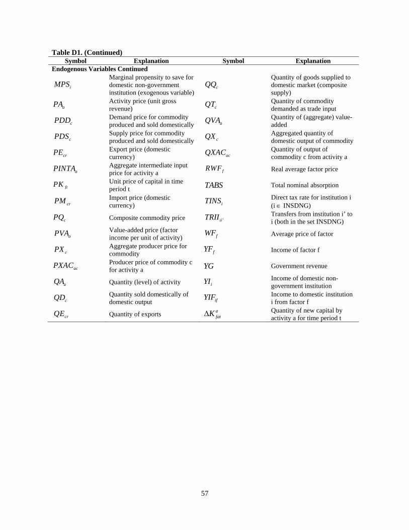
57

Table D1. (Continued) Symbol Explanation Symbol Explanation

Endogenous Variables Continued

Marginal propensity to save for domestic non-government institution (exogenous variable)

Quantity of goods supplied to domestic market (composite supply)

Activity price (unit gross revenue)

Quantity of commodity demanded as trade input

Demand price for commodity produced and sold domestically

Quantity of (aggregate) value-added

Supply price for commodity produced and sold domestically

Aggregated quantity of domestic output of commodity

Export price (domestic currency)

Quantity of output of commodity c from activity a

Aggregate intermediate input price for activity a Real average factor price

Unit price of capital in time period t Total nominal absorption

Import price (domestic currency)

Direct tax rate for institution i (i INSDNG)

Composite commodity price Transfers from institution i’ to i (both in the set INSDNG)

Value-added price (factor income per unit of activity)

Average price of factor

Aggregate producer price for commodity

Income of factor f

Producer price of commodity c for activity a Government revenue

Quantity (level) of activity Income of domestic non-government institution

Quantity sold domestically of domestic output

Income to domestic institution i from factor f

Quantity of exports Quantity of new capital by activity a for time period t

iMPS cQQ

aPA cQT

cPDD aQVA

cPDS cQX

crPE acQXAC

aPINTA fRWF

ftPK TABS

crPM iTINS

cPQ 'iiTRII

aPVA fWF

cPX fYF

acPXAC YG

aQA iYI

cQD ifYIF

crQE afatK

58

Table D1 (Continued) Production and Price Equations

(1)

(2)

(3)

(4)

(5)

(6)

(7)

(8)

(9)

(10)

(11)

(12)

(13)

(14)

(15)

(16)

c a c a aQINT ica QINTA

a c cac C

PINTA PQ ica

vavaaa

1-

va va vafa a f a f a f a

f F

QVA QF

1

1

'

va vaa ava vaf va vaf

faf a a f a f a f a f a f a f af F

W WFDIST PVA QVA QF QF

' ''

vanvan f af a

1-

van vanf a f a f f a f a

f F

QF QF

1

1

' ' '' '' ' '''

van vanf a f avan van

f f a f f a f a f f a f a f f a f af F

W WFDIST W WFDIST QF QF QF

a a aQVA iva QA

a a aQINTA inta QA

(1 )a a a a a a aPA ta QA PVA QVA PINTA QINTA

a c a c aQXAC QA

a ac acc C

PA PXAC

1

1accac

cac acc c a c a c

a A

QX QXAC

1

1

'

ac acc cac ac

ca c c a c a c a c a ca A

PXAC = QX QXAC QXACPX

''

cr cr c c cc CT

PE pwe EXR PQ ice

1tct t

c ct t tc cr crc cr c

r r

= + (1- )QX QE QD

1

1tc

tcr

crcr rt

c cc

1 - QE PE = QD PDS

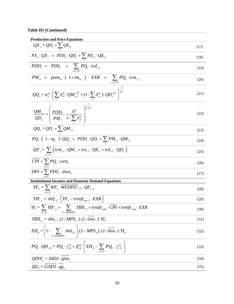
59

Table D1 (Continued) Production and Price Equations

(17)

(18)

(19)

(20)

(21)

(22)

(23)

(24)

(25)

(26)

(27)

Institutional Incomes and Domestic Demand Equations

(28)

(29)

(30)

(31)

(32)

(33)

(34)

(35)

c crcr

= QD QEQX

c c c c cr crr

PX QX PDS QD PE QE

' ''

c c c c cc CT

PDD PDS PQ icd

' ''

1cr cr cr c c cc CT

PM pwm tm EXR PQ icm

qq q cc c

1-

- -q q qc cr crc cr c

r r

= + (1- )QQ QM QD

qc

1

1+q

ccr cq

c crcr

QM PDD =1 - QD PM

c c crr

= QQ QD QM 1c c c c c cr cr

r

PQ tq QQ PDD QD PM QM

' ' ' ' ' '' '

c c c c c c c cc cc C

= icm QM ice QE icd QT QD

c cc C

CPI PQ cwts

c cc C

DPI PDS dwts

f af f f aa A

YF = WF WFDIST QF

i f i f f row fYIF = shif YF trnsfr EXR

'' '

i i f i i i gov i rowf F i INSDNG

YI = YIF TRII trnsfr CPI trnsfr EXR

'' ' ' 'ii i i i i iTRII = shii (1- MPS ) (1- tins ) YI

1 1 hh i h h hi INSDNG

EH = shii MPS (1- tins ) YI

' ''

m m mc c h c ch ch h c c h

c C

PQ QH = PQ EH PQ

c cQINV = IADJ qinv

c cQG = GADJ qg

60

Table D1. (Continued) Institutional Incomes and Domestic Demand Equations

(36)

System Constraints and Macroeconomic Closures

(37)

(38)

(39)

(40)

(41)

(42)

(43)

Capital Accumulation and Allocation Equations

(44)

(45)

(46)

(47)

(48)

(49)

c c i govc C i INSDNG

EG PQ QG trnsfr CPI

i i c c c cc ci INSDNG c CMNR c C

gov f gov rowf F

YG tins YI tm EXR tq PQ QQpwm QM

YF trnsfr EXR

c c a c h c c c ca A h H

QQ QINT QH QG QINV qdst QT

f a fa A

QF QFS

YG EG GSAV

cr cr row f cr cr i rowr c CMNR f F r c CENR i INSD

pwm QM trnsfr pwe QE trnsfr FSAV

1 ii i c c c ci INSDNG c C c C

MPS tins YI GSAV EXR FSAV PQ QINV PQ qdst

1i iMPS mps MPSADJ

'

f a taf t f t f a t

a f a' ta

QFAWF WF WFDIST

QF

,

'

1 1f a t f t f a ta af a t a

f a' t f ta

QF WF WFDIST

QF AWF

c t c ta a cf a t f a t

f t

PQ QINVK

PK

'

c tf t c t

c c' tc

QINVPK PQ

QINV

1af a t

f a t+1 f a t ff a t

KQF QF

QF

1 1f a t

af t f t f

f t

KQFS QFS

QFS

61

REFERENCES

Allen, R.G., L.S. Pereira, D. Raes, and M. Smith. 1998. Crop evapotranspiration - Guidelines for computing crop water requirements. FAO Irrigation and Drainage Paper No. 56, Rome, Italy: United Nations Food and Agriculture Organization

Alley, W.M. 1984. The palmer drought severity index: Limitations and assumptions. Journal of Climate and Applied Meteorology 23: 1100-1109.

Breisinger, C. and J. Thurlow. 2008. Asian-driven resource booms: Rethinking the impacts on African development. Discussion paper 747. Washington D.C: International Food Policy Research Institute.

Diao, X., P. Hazell, D. Resnick, and J. Thurlow. 2007. The role of agriculture in pro-poor growth in Sub-Saharan Africa. Research report 144. Washington D.C.: International Food Policy Research Institute.

Doorenbos, J. and A.H. Kassam. 1979. Yield response to water. Part A of FAO irrigation and drainage paper No. 33. Rome, Italy: Food and Agriculture Organization of the United Nations..

FAO, 1979. Yield response to water. Part B of FAO Irrigation and Drainage Paper No. 33. Rome, Italy: United Nations Food and Agriculture Organization. < http://www.fao.org/landandwater/aglw/cropwater/cwinform.stm> Accessed July 2009.

Houghton, J.T. 2004. Global warming: The complete briefing. Cambridge, UK: Cambridge University Press,

Hulme, M., ed. 1996. Climate change and Southern Africa. Climatic Research Unit, Norwich, UK: University of East Anglia.

IPCC. 2007a. Summary for policy makers. Climate Change 2007: Synthesis Report. Fourth assessment report of the intergovernmental panel for climate change, available at <http://www.ipcc.ch/pdf/assessment-report/ar4/syr/ar4_syr_spm.pdf> Accessed July 2009.

IPCC. 2007b. Climate change 2007: The physical science basis. Contribution of working group I to the fourth assessment report of the intergovernmental panel on climate change, S. Solomon, D. Qin, M. Manning, Z. Chen, M. Marquis, K.B. Averyt, M. Tignor M., and H.L. Miller, eds. Cambridge, UK and New York: Cambridge University Press.

Jensen, M.E. 1968. Water consumption by agricultural plants. In Water deficits and plant growth (II), T.T. Kozlowski, ed. New York: Academic Press.

Kipkorir, E.C. and D. Raes. 2002. Transformation of yield response factor into Jensen’s sensitivity index. Irrigation and Drainage Systems (16): 47-52.

Long, S.P., E.A. Ainsworth, A.D.B. Leakey, J. Nosberger, and D.R. Ort. 2006. Food for thought: lower-than-expected crop yield stimulation with rising CO2 concentrations. Science (312) 1918-1921.

Palmer, W.C. 1965. Meteorological drought. Research Paper No. 45. U.S. Weather Bureau. Washington D.C.: NOAA Library and Information Services Division. < http://www.ncdc.noaa.gov/oa/climate/research/drought/palmer.pdf >

Prairie, J.R., B. Rajagopalan, T.J. Fulp, and E.A. Zagon. 2006. Modified k-NN model for stochastic streamflow simulation. Journal of Hydrologic Engineering ASCE, 11(4): 371-378.

Resnick, D. and J. Thurlow. In press. Development strategies, macroeconomic policies, and the agricultural sector in Zambia. In Food policy for developing countries: The role of government in the global food system, P. Pinstrup-Andersen, and F. Cheng, eds. New York: Cornell University Press.

Rogers, P. 2008. Coping with global warming and climate change, Journal of Water Resources Planning and Management 134(3): 203-204.

Thurlow, J. 2005. A recursive dynamic computable general equilibrium model (CGE) for South Africa. Pretoria, South Africa: Trade and Industrial Policy Strategies.

62

Thurlow, J., S. Benin, X, Diao, H. Kalinda, and T. Kalinda. 2008 Agricultural growth and investment options for poverty reduction in Zambia. Discussion Paper 791. Washington D.C.: International Food Policy Research Institute.

Thurlow, J. and P. Wobst. 2006. Not All growth is equally good for the poor, Journal of African Economies, 15(4): 603-625.

Tsakiris, G.P., 1982. A method for applying crop sensitivity factors in irrigation scheduling. Agric. Water Manage 5: 335-343.

Verdin, J., C. Funk, G. Senay, and R. Choularton. 2005. Climate science and famine early warning. Philosophical Transactions of the Royal Society (B) 360: 2155-2168.

World Bank, 2008. An assessment of the economic impact of flood and drought events in Zambia. Washington D.C.: The World Bank (47).

Yates, D., H. Galbraith, D. Purkey, A. Huber-Lee, J. Sieber, J. West, S. Herrod-Julius, and B. Joyce. 2007. Climate warming, water storage, and Chinook salmon in California’s Sacramento Valley. Climatic Change 91(3-4): 335-350.

Zhu, T., Jenkins, M.W. and Lund, J.R. 2005. Estimated impacts of climate warming on California water availability under twelve future climate scenarios. Journal of the American Water Resources Association 41(5): 1027-1038.

63

RECENT IFPRI DISCUSSION PAPERS

For earlier discussion papers, please go to www.ifpri.org/pubs/pubs.htm#dp. All discussion papers can be downloaded free of charge.

889. Navigating the perfect storm: Reflections on the food, energy, and financial crises. Derek Headey, Sangeetha Malaiyandi, and Shenggen Fan, 2009.

888. How important is a regional free trade area for southern Africa? Potential impacts and structural constraints. Alejandro Nin Pratt, Xinshen Diao, and Yonas Bahta, 2009.

887. Determinant of smallholder farmer labor allocation decisions in Uganda. Fred Bagamba, Kees Burger, and Arie Kuyvenhoven, 2009.

886. The potential cost of a failed Doha Round. Antoine Bouët and David Laborde, 2009.

885. Mapping South African farming sector vulnerability to climate change and variability: A subnational assessment. Glwadys Aymone Gbetibouo and Claudia Ringler, 2009.

884. How does food price increase affect Ugandan households? An augmented multimarket approach. John M. Ulimwengu and Racha Ramadan, 2009.

883. Linking urban consumers and rural farmers in India: A comparison of traditional and modern food supply chains. Bart Minten, Thomas Reardon, and Anneleen Vandeplas, 2009.

882. Promising Approaches to Address the Needs of Poor Female Farmers: Resources, Constraints, and Interventions. Agnes R. Quisumbing and Lauren Pandolfelli, 2009.

881. Natural Disasters, Self-Insurance, and Human Capital Investment: Evidence from Bangladesh, Ethiopia, and Malawi. Futoshi Yamauchi, Yisehac Yohannes, and Agnes Quisumbing, 2009.

880. Risks, ex-ante actions, and public assistance: Impacts of natural disasters on child schooling in Bangladesh, Ethiopia, and Malawi. Futoshi Yamauchi, Yisehac Yohannes, and Agnes Quisumbing, 2009.

879. Measuring child labor: Comparisons between hours data and subjective measures. Andrew Dillon, 2009.

878. The effects of political reservations for women on local governance and rural service provision: Survey evidence from Karnataka. Katharina Raabe, Madhushree Sekher, and Regina Birner, 2009.

877. Why is the Doha development agenda failing? And what can be Done? A computable general equilibrium-game theoretical approach. Antoine Bouët and David Laborde, 2009.

876. Priorities for realizing the potential to increase agricultural productivity and growth in Western and Central Africa. Alejandro Nin-Pratt, Michael Johnson, Eduardo Magalhaes, Xinshen Diao, Liang You, and Jordan Chamberlin, 2009.

875. Rethinking China’s underurbanization: An evaluation of Its county-to-city upgrading policy. Shenggen Fan, Lixing Li, and Xiaobo Zhang, 2009.

874. Agricultural trade liberalization and poverty in Brazil. Joachim Bento de Souza Ferreira Filho, 2009.

873. Economywide impacts of climate change on agriculture in Sub-Saharan Africa. Alvaro Calzadilla, Tingju Zhu, Katrin Rehdanz, Richard S.J. Tol, and Claudia Ringler, 2009.

872. Decentralization and local public services in Ghana: Do geography and ethnic diversity matter? Kamiljon T. Akramov and Felix Asante, 2009.

871. Soil and water conservation technologies: A buffer against production risk in the face of climate change? Insights from the Nile Basin in Ethiopia. Edward Kato, Claudia Ringler, Mahmud Yesuf, and Elizabeth Bryan, 2009.

870. Validation of the World Food programme’s food consumption score and alternative indicators of household food security. Doris Wiesmann, Lucy Bassett, Todd Benson, and John Hoddinott, 2009.

869. Rebuilding after emergency: Revamping agricultural research in Sierra Leone after civil war. Kwadwo Asenso-Okyere, Sindu Workneh, Edward Rhodes, and John Sutherland, 2009.

INTERNATIONAL FOOD POLICY RESEARCH INSTITUTE

www.ifpri.org

IFPRI HEADQUARTERS

2033 K Street, NW Washington, DC 20006-1002 USA Tel.: +1-202-862-5600 Fax: +1-202-467-4439 Email: [email protected]

IFPRI ADDIS ABABA

P. O. Box 5689 Addis Ababa, Ethiopia Tel.: +251 11 6463215 Fax: +251 11 6462927 Email: [email protected]

IFPRI NEW DELHI

CG Block, NASC Complex, PUSA New Delhi 110-012 India Tel.: 91 11 2584-6565 Fax: 91 11 2584-8008 / 2584-6572 Email: [email protected]

Documents

The Impact of Climate Variability and Change on Economic ... · impacts of climate variability and change on economic growth and poverty reduction in Zambia. The hydro-crop model