The Impact of Adoption of Wrongful Discharge Laws on Wages

1

The Impact of Adoption of Wrongful Discharge Laws on Wages: 1979-2014

Dissertation Paper 2

15 March 2018

Eric Hoyt, Tufts University Visiting Scholar,

University of Massachusetts Amherst Economics Doctoral Candidate

Abstract:

While economic theory offers predictions about the effect of employment protection on wages,

the empirical literature has focused primarily on employment effects. This paper uses

individual-level panel data from the National Longitudinal Survey of Youth 1979 and weighted

ordinary least squares and unconditional quantile difference-in-differences regressions to

estimate the effect of wrongful discharge laws, a court-based form of employment protection in

the United States, on average, and across the marginal distribution of, real wages. I find that one

wrongful discharge law, the good faith doctrine, increases average real wages by 18.59 percent

for all private-sector non-self-employed workers, 17.18 percent for nonmanufacturing workers,

13.75 percent for men, 21.68 percent for women, 21.04 percent for white workers, and 12.97

percent for nonwhite workers. My results show that wrongful discharge laws, whether by

increasing workers’ bargaining power or by increasing their labor productivity, can boost

workers’ wages, particularly for women, minorities, and workers in nonmanufacturing industries

who have been hardest hit by recent economic changes.

Keywords: wages, unconditional quantile regression, wrongful discharge laws, employment

protection

Acknowledgements: I am grateful for the guidance of Professors Fidan Kurtulus, Gerald

Friedman, and Eve Weinbaum as well as for the numerous helpful comments of professors and

fellow graduate students at the University of Massachusetts Amherst.

Author Contacts: [email protected], Room 101 Dearborn House, 72 Professors Way,

Tufts University, Medford, MA 02155, (413)-362-4517

2

3

I. Introduction

Employers’ ability to fire workers has been a major focus in the literature studying

different patterns of employment and growth in the United States and Europe. Wrongful

discharge laws, a form of court-based employment protection in the United States, have been a

special focus of this literature, as their adoption randomly across state and time from the 1970s

through 1990s creates numerous natural experiments regarding the impact of employment

protection on labor markets. While much focus has been put on the effect of these increased

firing costs on employment, less time has been spent investigating the impact on wages, even

though theoretical literature on employment protection makes clear predictions about the impact

of firing costs on wages.

There have been three primary wrongful-discharge doctrines that have proliferated in recent

decades: the implied contract doctrine, the public policy doctrine, and the covenant of good faith

and fair dealing. The implied contract doctrine states that language in employee manuals and

oral promises made by supervisors detailing a specific duration of employment or standard

procedures for dismissal can override the default of employment-at-will. The public policy

doctrine is an exception to the at-will rule that arises when an employee is discharged after

invoking a publicly protected right or obligation, such as filing a worker’s compensation claim or

attending jury duty, or refusing an employer’s request to break the law. Finally, the good faith

doctrine, if followed to the letter, requires that every discharge decision be justified. While in

some states it has maintained this broad meaning, in many states the good faith doctrine in later

years was revised to, like the public policy doctrine, only to prohibit particular cases of morally

reprehensible termination. The implied contract and public policy doctrines were adopted by 43

states, the good faith doctrine was adopted by 12 states, with the earliest policy adoption in 1959

4

and the latest in 1994. There have been few complete repeals of wrongful discharge laws, so that

as of 2014, 42 states recognized the implied contract doctrine, 43 states recognized the public

policy doctrine, and 11 states recognized the good faith doctrine.

Using the National Longitudinal Survey of Youth 1979 panel data and the Current

Population Survey Monthly Outgoing Rotation Group files for the years 1979 through 2014 and

weighted ordinary least squares difference-in-difference regression, I find that the good faith

doctrine significantly raises average real wages by 18.59 percent for all private-sector non-self-

employed workers, 17.18 percent for nonmanufacturing workers, 13.75 percent for men, 21.68

percent for women, 21.04 percent for white workers, and 12.97 percent for nonwhite workers.

Using the same dataset for the same years but a difference-in-differences unconditional quantile

regression methodology, I find significant increases across the marginal distribution of real

wages, especially for median real wages for all private-sector non-self-employed workers of

21.07 percent, for nonmanufacturing workers of 24.05 percent, for men of 21.07 percent, for

women of 20.02 percent, for white workers of 23.67 percent, and for nonwhite workers of 15.77

percent. I also find that the good faith doctrine lowers the probability by 5 percent that women

workers have real wages that would bring a family of two (one adult and one child) an income

less than or equal to the federal poverty level, and lowers the probability by 7 percent that

women workers have real wages sufficient to bring a family of three (one adult and two children)

an income less than or equal to 125 percent of the federal poverty level. Finally, I also find that

one other wrongful discharge law, the implied contract doctrine, significantly increases average

real wages by 4.77 percent, and increases the bottom 40% of the marginal distribution of

manufacturing worker real wages by 7.78 percent.

5

The standard supply-and-demand model of the labor market predicts that employment

protection policies will cause a decrease in wages, provided the increase in firing costs is not

offset by an increase in marginal productivity of labor. Labor demand shifts inward, so, all else

constant, the equilibrium wage will decline. However, as Autor et. al. 2006 and Blanchard and

Portugal (2001) explain, by increasing workers’ bargaining power vis-à-vis employers,

employment protection can also allow workers to prevail in bargaining over wage hikes,

especially in worksites paying non-competitive efficiency wages. Thus, in effect, labor supply

might shift inward. Autor et. al. (2006) find no statistically significant effect on wages following

state adoption of wrongful discharge laws in the U.S. over the 1980s and 1990s, and posit that,

given their disemployment findings reflecting an inward demand shift, the lack of a negative

wage effect suggests a countervailing inward supply shift driven by workers’ increased power in

bargaining over wage demands.

One important reason I do not limit this investigation solely to the Current Population Survey

Monthly Outgoing Rotation Group files, as done by Autor et. al (2006), is because this data is

made up of repeated pooled cross-sections that may be biased by compositional shifts associated

with policy adoption. I use the National Longitudinal Survey of Youth 1979 panel data to permit

the analysis of changes in individual workers’ wages before and after policy change, as well as to

control for firm-size, in contrast to the Current Population Survey Monthly Outgoing Rotation

Group files which are cross-sectional and do not contain information on the firms in which

workers are employed. Firm size, given the institutional peculiarities of wrongful discharge laws

is an important factor in the degree to which the policies actually apply in practice to workers.

Large firms, who have the resources to retain management lawyers, are able to contract around

and outmaneuver wrongful discharge laws while small firms are often caught off guard and more

6

likely to face the full cost of these policies. Autor et. al. (2007), which analyzes the impact of

wrongful discharge laws on productivity using industry state year panel data with firm fixed

effects, incorporates firm-level fixed effects and finds that adoption of the good faith doctrine is

associated with significant increases in labor productivity, a result that mirrors, and helps

explain, the positive significant effect of the good faith doctrine on wages found in this study.

Another reason the adoption of the good faith doctrine has strong effects on productivity and

wages may be because it occurs more sporadically across state and year, so it is harder for firms

to anticipate, yielding stronger and more discrete effects on labor market outcomes. Given my

inclusion of firm size controls, as well as the ability to track the changes in individual workers’

wages overtime, my wage results differ from those in Autor et. al. (2006) in terms of significant

positive effects following adoption of the good faith doctrine, though I similarly find little wage

effects associated with adoption of the implied contract and public policy doctrines.

II. Previous Literature

Van der Wiel (2010) uses a 1999 reform to Dutch labor law that increased the period of

notice required for dismissal for younger and less tenured workers while decreasing that required

for older and higher seniority workers, in order to analyze the effect of employment protection

on wages. She proposes the standard prediction of falling wages from an inward shift in labor

demand. However, she also posits that wages might increase because of rising worker

bargaining power, citing Bertola (1990), represented by an inward shift of labor supply, or

because of rising labor productivity fueled by investment in worker skill acquisition or capital,

and denoted by an outward shift of label demand. This last explanation, while understudied, is

nonetheless echoed in the textbook discussion of employment protection found in Nickell and

Layard (1999), and, as mentioned above, may help explain the similarity between the results in

7

Autor et. al. (2007) and the present paper of, respectively, rising labor productivity and wages

following good faith doctrine adoption.

Van der Wiel performs a fixed effects difference-in-differences regression to investigate

the impact of policy change on real wages, and finds an increase of between 3% and 5%, with

greater increases for lowest-skilled workers. She also performs a probit model analysis on the

impact of policy adoption on the probability a worker enrolls in job training, and finds a roughly

7% significant decline. These results together suggest that, at least in the Dutch context of

centralized collective bargaining over wages between organized labor and employer federations,

the bargaining power, rather than skill or capital investment, explanation of wage hikes from

employment protection seems most plausible. Given low unionization and bargaining power, but

high skill-level, of U.S. workers, Van der Wiel’s analysis motivated my interest in investigating

if any wage increases follow wrongful discharge law adoption, and whether these increases are

motivated by increased bargaining power or investment in skill or capital.

Leonardi and Pica (2010), investigating a policy which provided severance to small firms

in Italy, estimate the effect of employment protection on wages for high and low bargaining

power demographics and find negative effects on wages, especially for younger, less tenured,

and blue-collar workers. These results contrast somewhat with those in this paper, in so far as I

find that women’s wage gains outstrip those of men, and nonmanufacturing workers’ wage gains

surpass those of manufacturing workers. However, there is some similarity in that the increases

for white workers are greater than those for nonwhite workers, that negate wage effects occur at

the very bottom of the marginal distribution of real wages, and significant increases in wages

occur steadily in magnitude moving up the marginal distribution of real wages. One reason for

the discrepancies in results by demographic group between this analysis and those of Leonardi

8

and Pica (2010) may be that the increases in wages brought by the good faith doctrine might

reflect the role of training and learning-by-doing in boosting labor productivity, rather than

solely the impact of increased worker bargaining power, which would bias wage increases

toward workers the highest wages prior to policy adoption.

My paper adds to the literature on the impact of employment protection on labor markets

by being the first, as far as I’ve seen in my survey of literature, to investigate the impact of

wrongful discharge laws on wages by gender, race, and education, by more detailed industrial

categories, and by quantiles of the marginal distribution of wages. My results show that

wrongful discharge laws, whether by increasing workers’ bargaining power or by increasing

their labor productivity, can boost workers’ wages, particularly for women, minorities, and

workers in nonmanufacturing industries who have been hardest hit by recent economic changes.

The evidence that the good faith doctrine lowers the likelihood that women earn wages providing

income at or near to the federal poverty level is especially important, given the large and

growing share of single female heads of households in the United States. For instance, as a

recent investigation by Pew (2015) found that, while in 1960, 5% of all children were born to

single female heads of households, the number has steadily increased and stabilized at 40% by

2014. These families had median annual income of $24,000 in 2014, while married families

with male breadwinners had median annual income of $84,500.

III. Data Sources

A. NLSY79

My primary data source is the National Longitudinal Survey of Youth 1979 (hereafter

NLSY79), a yearly panel of 12,682 men and women who were between the ages of 14 and 22 in

the year 1979, containing data on a range of information about individuals’ life histories,

working conditions, and personal beliefs from 1979 to present. I construct my outcome variable

9

of real hourly wage in one’s primary job, using real year 2000 U.S. dollars and the Consumer

Price Index for Urban Wage Earners and Clerical Workers. Following the common practice

within research on wages, I drop observations for wages below $1.50 per hour or above $100 per

hour. I pull demographic information from the data set to construct indicator variables for

gender (male vs. female), age (14-24 vs. 25-58), education (high school or less vs. at least some

college), and race (white vs. nonwhite). I extract data on industry classification of workers’

primary jobs to construct indicators for employment within construction, manufacturing,

transportation, communication, utilities, health care and social services, wholesale trade, and

retail trade industries. I create dummies for the size of the firm in which workers’ primary jobs

reside, measured in terms of the total number of employees (0-19 vs. 20-49 vs. 50-99 vs. 100 and

above) per firm. Finally, I construct indicators for census region and state of workers’ residence

from the restricted use geocode files which I was given access to by the U.S. Bureau of Labor

Statistics. I drop data for self-employed and public-sector workers, since wrongful discharge

laws apply only to private sector employees who are employed by a business or individual other

than themselves.

B. CPS MORG

In order to perform a sensitivity analysis on my NLSY79 wage research, as well as to

gather sufficient data to investigate effects within the important nonmanufacturing industries of

transportation and communications, I draw upon the Current Population Survey Merged

Outgoing Rotation Group files (hereafter CPS-MORG) for 1979-2013. I construct my main

outcome variable of real wages as the usual weekly earnings divided by usual weekly hours,

adjusted by the Consumer Price Index for Urban Wage Earners and Clerical Workers to convert

observations to real year 2000 U.S. dollars. As in the first data set, I drop observations for wages

10

below $1.50 per hour and above $100 per hour, as well as for workers who are self-employed or

employed by the public sector in their primary job. I pull demographic data to construct

dummies for gender (male vs. female), age (16-39 vs. 40-64), education (high school or less vs.

at least some college), and race (white vs. nonwhite). I construct industry indicators for workers’

primary employment in construction, manufacturing, transportation, communication, utilities,

health care and social services, wholesale trade, and retail trade. I also pull geographic

information to construct indicators for state and census region of workers’ residence.

C. Legal Variables

This paper uses state court decisions from 1970 through 2014 to construct explanatory

variables on wrongful discharge doctrine adoptions. I employ the method of Morris (1995),

which was adopted by Autor et. al. (2006) for the years 1970 through 1999, by coding the first

state Supreme Court or Intermediate Appellate court ruling that demonstrates a clear acceptance

of each of the three wrongful discharge doctrines. I construct legal adoption variables at the

yearly-level from 1979 to 2014 to match the NLSY79, and on a monthly basis from the year

1979 through 2013, in order to match data available at the monthly-level for these years from the

CPS-MORG files. Both forms of this data set contain the sustained (i.e. at least five-year long)

adoption of the implied contract doctrine by 36 states, the public policy doctrine by 36 states, and

the good faith doctrine by 10 states.

IV. Econometric Models

A. Difference-in-Differences Regression

1. OLS

Since state adoption of wrongful discharge laws is an idiosyncratic function of the

decisions of State Supreme Court and Intermediate Appellate Court justices, as well as of the

cases that emerge and rise to the docket of these courts, I have numerous natural experiments

11

over the 1980s and 1990s to investigate the effect of employment protection on workers’ wages.

My main specification is the following weighted OLS fixed effects regression of log real hourly

earnings, similar to that implemented by Autor et. al. (2006) in their analysis of the impact of

wrongful discharge laws on average real wages:

wijstdf = β1Treatst + β2Postst + β3TreatstPostst + γs + δt + πj

+ κd + λf + θi + β4 Postpostst + δt x Regiont + εijstdf (1)

where wijstdf is 100 times the log real hourly wage of individual i, in state s, at year t, in industry

d, and within a firm of size f.

Treatst is an indicator for the five-year period from 2 years before to 2 years after the year

of adoption of a wrongful-discharge law in adopting state s. Postst is an indicator for the period

from the year of adoption through 2 years after the year of adoption for all states, both adopting

and nonadopting. TreatstPostst is an interaction term representing the three-year period

following policy adoption in the treatment state only. Postpostst is a dummy variable that

represents each state that reenters the control group 3 years after the year of policy adoption to

account for any bias caused by enduring effects. These window lengths are the same as the

windows in Autor et. al. (2006) for consistency1.

1 To illustrate the legal doctrine adoption variables, consider the following example. Massachusetts adopted the

implied contract doctrine in 1988, while neighboring Rhode Island did not adopt any wrongful discharge law over

the period studied. Massachusetts is a treatment state, so the variable Treatst takes on the value one for the years

1986, 1987, 1988, 1989, and 1990, and takes on the value of zero in years before 1986 and after 1990. Since Rhode

Island did not adopt any wrongful discharge law over the five years surrounding adoption of the implied contract

doctrine in Massachusetts, Treatst always remains zero in this state. In this case, Rhode Island is included within the

control group. The variable Postst takes on the value one in Massachusetts and Rhode Island, and in all other states,

for all years that this policy remains in effect in Massachusetts, beginning with the year of adoption, which in this

case is the year 1988 to the end of the dataset in 2014. Treatst* Postst is an interaction term representing the three-

year period, in the treatment state only (i.e. Massachusetts), beginning with the year of adoption of the implied

contract doctrine in 1988. In other words, Treatst* Postst takes on the value one only in Massachusetts and only for

the years 1988, 1989, and 1990. Maine, another neighboring state, also did not adopt any wrongful discharge laws

over the five years surrounding 1988, so it is included within the control group. However, Maine adopted the

implied contract doctrine in 1978. In this case, the variable PoststPostst switches from zero to one for Maine starting

the year after the treatment window for its adoption ended, which is 1981, and takes on the value one for the rest of

sample period until 2014. If Massachusetts becomes eligible as a control for a later state adoption, its PoststPostst

12

The coefficient of interest β3 is an estimate of the pre-post change in the outcome variable

in adopting states relative to the corresponding change in non-adopting states. Identification of β3

comes from variation in real wages between adopting and nonadopting states over the five years,

two before to three years after, policy adoption within U.S. Census region, industry,

demographic, and firm size groups. This specification gives an estimate of the causal effect of

policy adoption controlling for a variety of state, regional, national, industry, firm-size, and year-

specific characteristics that influence wages and are correlated with policy adoption. Over the

years 1979 through 2014, and economy-wide, real wages in the NLSY79 sample have a mean of

$12.18, median of $9.79, standard deviation of $8.39, and variation of $70.41 in U.S. year 2000

dollars per hour.

The variable αs is a state intercept that captures idiosyncratic, unobserved, and pre-

existing features of each relevant state which might impact wages irrespective of the year of

observation. δt are fixed time effects which control for yearly state-invariant shifts in the

regression intercept, accounting for common national shocks to wages. δt x Regions are

interactions of the four U.S. Census regions with year fixed effects, and control for transitory

regional shocks to wages. πj is a vector of demographic group indicators for sixteen

demographic groups [i.e. (male vs. female) X (ages 14-24 vs. 25-58) X (high school or less vs. at

least some college) X (white vs. nonwhite)]. κd are indicator variables representing the industry

in which a worker’s primary employment resides as defined by eight major industrial

classifications (i.e. construction, manufacturing, transportation, communication, utilities, health

care and social services, wholesale trade, or retail trade industries). λf represents dummies for

variable, which switches on beginning in 1991, would take on the same role as it plays in Maine in this example.

One important consequence of this five year treatment window structure for the fixed effect specification is that it

omits analysis of policy adoptions occurring from 1979 and 1980.

13

four categories of firm size (i.e. total number of employees per firm of 0-19 vs. 20-49 vs. 50-99

vs. 100 and above). θi is an indicator for if an individual ever moves from one state of residence

to another during the sample time period, and controls for unobservable characteristics of movers

that might impact wages. Each regression is weighted using NLSY79 sample weights. Huber-

White robust standard errors are used to account for within-state error correlations. In

regressions using only data within industry subsamples, the indicators for workers’ industry of

primary employment κd are necessarily dropped. In regressions using only data within

demographic group subsamples, the vector of indicator variables for demographic characteristics

of workers πj are necessarily dropped.

In the sensitivity analysis using the CPS-MORG data set, I use a version of specification

1 that is identical aside from the vector of demographic dummies, πj, having a higher distinction

between younger and older workers (i.e. ages 16-39 vs. 40-64 as opposed to ages 14-24 vs. 25-

58), since the average age is higher in the CPS-MORG cross-sectional data than the youth-

focused household survey data of the NLSY79. Also, since the CPS-MORG does not contain

information on the size of firms in which workers are employed, this version of specification 1

does not contain indicators for firm size, λf. This final distinction is especially significant, and

one reason my analysis using NLSY79 contributes to research on wrongful discharge laws, as

there is reason to believe, as Autor et. al. (2007) highlight, that larger firms are more likely than

smaller firms to anticipate and contract around wrongful discharge laws, as they have resources

to retain skilled company lawyers, who often advise against establishing company policies and

practices that would create employment protection under wrongful discharge law protections, or

who might recommend proactive actions to subvert these protections such as including

employment-at-will disclaimers within employee handbooks. These regressions use CPS

14

earnings weights. Huber-White robust standard errors clustered at the state-level are used to

account for within-state error correlations. In regressions using only data within demographic

group subsamples, the vector of indicator variables for demographic characteristics of workers πj

are necessarily dropped, and in regressions using only data within industry subsamples, the

indicators for industry of primary employment κd are dropped.

2. Unconditional Quantile Regression

In order to investigate the impact of wrongful discharge laws on the quantiles of the

marginal distribution of wages I employ unconditional quantile regression, which, as developed

by Firpo et. al. (2009), operationalizes estimation using a recentered-influence function

(hereafter RIF) of the outcome variable. The RIF for the τth quantile, Qτ, is defined as:

𝑅𝐼𝐹(𝑤𝑖𝑗𝑠𝑡𝑑𝑓, 𝑄𝜏) = [𝑄𝜏 +𝜏

𝑓(𝑄𝜏)] −

1(𝑦𝑖𝑡 < 𝑄𝜏)

𝑓(𝑄𝜏)= 𝑘 𝜏 −

1(𝑦𝑖𝑡 < 𝑄𝜏)

𝑓(𝑄𝜏)

I estimate the following regression for every decile, 𝑄𝜏 = 0.10 to 𝑄𝜏 = 0.90, using the same

difference in difference estimation methodology for wrongful discharge policy adoptions as

employed for average effects in equation 1:

RIF(wijstdf ,Qτ) = β1Treatst + β2Postst + β3TreatstPostst + γs + δt + πj

+ κd + λf + θi + β4 Postpostst + δt x Regiont + εijstdf (2)

Equation 2 is identical in all respects to equation 1, aside from the implementation of the RIF

methodology using the dependent variable. The same distinctions hold as before regarding the

higher age cut-off within the age demographic indicator variable, the dropping of firm-size

indicator variables, and the substitution of CPS earnings weights for NLSY79 yearly sample

weights when employing this specification in the CPS-MORG data versus the NLSY79 data set,

as was the case in equation 1. Huber-White robust standard errors clustered at the state-level are

used to account for within-state error correlations. In regressions using only data within

15

demographic group subsamples, the vector of indicator variables for demographic characteristics

of workers πj are necessarily dropped, and in regressions using only data within industry

subsamples, the indicators for industry of primary employment κd are dropped.

B. Unconditional Quantile Regression with Leads and Lags

To give some picture of the dynamics effects of wrongful discharge doctrines on wages over

the years leading up to and following policy adoption, I utilize a base line differences-in-

differences regression with yearly leads and lags from two years before to three years after

adoption, which is similar to the dynamic specification included in Autor et. al. (2006), but

differs in containing the recentered-influence function of real wages, in order to investigate the

impact of adoption on low-waged workers within manufacturing industry. Specifically, I use the

following specification, evaluated at Qτ = 0.4, to analyze the impact on the bottom 40% of the

manufacturing marginal distribution of wages:

RIF(wijstdf ,Qτ = 0.4) = ∑ 2𝑚=−2 ηm Ls,t-m + γs + δt + πj + λf + θi + δt x Regions+ ԑijstdf (3)

All variables are as in equations 1 and 2, aside from the dummy variable Ls,t , which switches on

from zero to one only during the year a state court adopts a wrongful discharge doctrine, and

permits the estimation of the impact over the first year following adoption of each doctrine on

real wages in adopting states relative to nonadopting states. The parameter of interest ηm gives

the first-year impact of the adoption of wrongful discharge laws on the change in real wages

between adopting and nonadopting states. Identification of ηm comes from within region, within

industry, within demographic group, within firm size, and within mover and nonmover group

variation in real wages between adopting and nonadopting states. In order to match the results

for the full fixed-effects regression, the overall sample window of adoptions analyzed was

restricted to 1981 through 2011, ensuring the overall number of adoptions actually studied

16

remains the same (i.e. implied contract doctrine by 36 states, the public policy doctrine by 36

states, and the good faith doctrine by 10 states). As I use data from NLSY79, my main data set

for analysis, this specification contains variables on firm-size and mover vs. nonmover status,

and uses the lower age cut-off within the demographic indicator variables. Since it is a

regression using the manufacturing subsample, I necessarily drop the indicator for industry of

primary employment. The specification is weighted by NLSY79 sample weights, and uses

Huber-White robust standard errors clustered at the state-level.

C. Probit Model

Finally, I use the following reduced form probit model, similar to that implemented in Kugler

(2004), on the subsection of my NLSY79 sample that are women:

Pr(yijstdf , γs, δt, πj, κd, λf, θi,δt x Regions) = Φ(β1 dst + γs + δt + κd + λf + θi + δt x Regions) (4)

The dependent variable, yijstdf, represents two separate but similar dichotomous outcomes

measuring, respectively, whether a woman’s real hourly wage is less than or equal to $6.81 per

hour in year 2000 U.S. dollars, the wage which is sufficient to provide a family of two (i.e. one

parent and one child) an income equal to the federal poverty level, and whether a woman’s real

hourly wage is less than or equal to $9.94 per hour in year 2000 U.S. dollars, that which is

sufficient to provide a family of three (i.e. one parent and two children) an income equal to 125

percent of the federal poverty level. This specification includes all of the same right-hand-side

variables as equation 1, with the exception that the legal adoption variable, dst, captures the effect

of each wrongful discharge law over the entire time period they are in effect, which in most cases

represents the period from adoption until then end of the sample in 2014. In this instance, β1, the

coefficient of interest, provides an estimate of the direct effect of wrongful discharge laws on the

probability women have poverty-level or close to poverty-level wages. Since the regression is

17

performed using the subsample of women workers, the vector of demographic group categories

πj is necessarily dropped. The specification is weighted by NLSY79 yearly sample weights, and

uses Huber-White robust standard errors clustered at the state-level.

V. Results

A. Event Study Difference-in-Differences Regression: NLSY79 sample

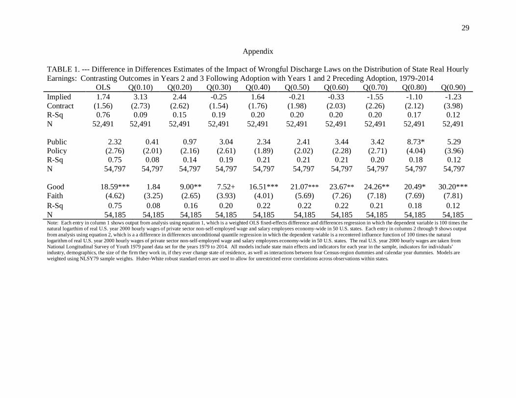
The first column of Tables 1 through 7 show estimates of the impact of wrongful

discharge laws on average wages, using the coefficient of interest β3 of the OLS fixed-effects

difference-in-differences methodology of equation 1, while the second through ninth columns

show the effect upon the marginal distribution of real wages, using the coefficient of interest β3

of the difference-in-differences unconditional quantile regression framework of equation 2.

Table 1 illustrates results for all private sector non-self-employed workers, while Tables 2

through 7 show findings for specific industry and demographic group subsamples. While some

interesting differences in magnitude and significance of impact occur across industries,

demographic groups, and wage deciles, the general image that emerges is of a statistically

significant positive effect of the good faith doctrine upon wages, both on average and across the

marginal distribution.

1. Economy-wide

Table 1 reveals that adoption of the good faith doctrine is associated with significant

increases in real wages for all workers on average by 18.59 percent, and from the bottom 20

percent to the top 90 percent of the marginal distribution of real wages. It shows an increase of

9.00 percent for the bottom 20 percent of the real wage distribution, 21.07 percent for the

median, and the largest increase of 30.20 percent for the highest decile of the real wage

distribution. It shows no significant impact of the implied contract or public policy doctrines on

18

real wages, save a modestly significant increase in wages for the top 80 percent of the real wage

distribution following adoption of the public policy doctrine of 8.73 percent.

2. Female

Table 2 shows that the good faith doctrine increases average real wages for women

workers by 21.68 percent, and this is driven by significant, though varying in magnitude,

increases across every decile of the marginal distribution of women’s real wages. For instance,

the good faith doctrine raises real wages by 13.06 percent for the bottom 10 percent of the

distribution of women’s real wages, increases the median of women’s real wages by 20.02

percent, and has the largest increase for the top 80 percent of women’s real wages by 34.92

percent. While there is no impact, on the whole, from the implied contract and public policy

doctrine, the implied contract doctrine raises the very bottom decile of women’s real wages by

5.57 percent, and the public policy doctrine raises the very top decile of women’s wages by

11.87 percent.

3. Male

Table 3 illustrates that the good faith doctrine raises average real wages for men by 13.75

percent. While the good faith doctrine lowers the bottom 10 percent of men’s real wages by

11.66 percent, it increases the bottom 30 percent to the top 90 percent of their marginal

distribution of real wages. For instance, the good faith doctrine increases the bottom 30 percent

of men’s real wages by 10.15 percent, the median by 21.07 percent, and the top 60 percent by

26.33 percent. In so far as male workers at the very low-end of the wage distribution experience

wage declines, these results provide some evidence of a bargaining power effect, as illustrated by

Leonardi and Pica (2010), because workers with lower pre-policy adoption pay are unlikely to

have the initial bargaining power needed to make use of wrongful discharge laws in securing

19

wage gains from their employers. Although the implied contract doctrine has a marginally

significant positive effect on men’s average real wages, and the public policy doctrine has a

marginally significant positive effect on the top 80 percent of men’s marginal distribution of real

wages, the results are broadly consistent with previous findings of little significant effect of these

two policies on wages.

4. White

Table 4 shows the impact of wrongful discharge laws on the real wages of white workers.

It shows that the good faith doctrine increases average real wages for white workers by 21.04

percent, as well as the wages of white workers from the bottom 20 percent to the top 90 percent

of their marginal distribution of real wages, with an 11.41 percent increase for the second decile,

a 23.67 percent increase for the median, and the largest increase of 34.20 percent for the top 90

percent. There is no significant effect of either the implied contract doctrine or the public policy

doctrine on the real wages of white workers.

5. Nonwhite

In comparison, Table 5 reveals the impact of wrongful discharge laws on the real wages

of nonwhite workers. It shows that the good faith doctrine increases average real wages for

nonwhite workers by 12.97 percent, decreases real wages for the very lowest 10 percent of their

marginal distribution of real wages, but increases the bottom 30 percent to top 90 percent of their

marginal distribution of real wages. The good faith doctrine increases the bottom 30 percent of

the marginal distribution of nonwhite workers’ real wages by 13.13 percent, the median by 15.77

percent, and the top 90 percent by 37.70 percent. The magnitude of impact for nonwhite workers

is less than for white workers, and differs in showing declines for the very lowest decile, further

suggesting the importance of bargaining power differentials in explaining patterns of wage gains

20

following wrongful discharge law adoption. The implied contract doctrine has a marginally

significant positive effect on average nonwhite workers’ wages of 3.78 percent, for the bottom

20 percent of the marginal distribution of nonwhite workers’ real wages of 6.47 percent, and for

the bottom 30 percent of 6.17 percent. The public policy doctrine has a statistically significant

positive effect on nonwhite workers’ average real wages of 4.77 percent, for the lowest decile of

7.05 percent, for the bottom 30 percent of 6.55 percent, and for the top 90 percent of 13.66

percent.

6. Nonmanufacturing

Table 6 shows the impact of wrongful discharge laws on nonmanufacturing workers. It

reveals that the good faith doctrine increases average wages for nonmanufacturing workers by

17.18 percent, and increases nonmanufacturing workers real wages from the bottom 20 percent

to the top 90 percent of their marginal distribution. For instance, the good faith doctrine

increases the bottom 20 percent of the nonmanufacturing workers’ marginal distribution of real

wages by 5.77 percent, the median by 24.05 percent, and the top 90 percent by 28.16 percent.

The implied contract and public policy doctrines have no significant impact on

nonmanufacturing workers’ real wages.

7. Manufacturing

Table 7 shows the impact of wrongful discharge laws on manufacturing workers’ wages.

While the good faith doctrine has a marginally significant positive impact on average real wages

of manufacturing workers of 10.95 percent, it has a marginally significant negative effect of

11.44 percent on the real wages of the very bottom decile of manufacturing workers’ marginal

distribution of real wages. It also has a significant negative effect on the bottom 20 percent of

manufacturing workers’ marginal distribution of real wages of 9.51 percent, and significant

21

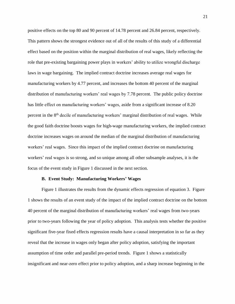
positive effects on the top 80 and 90 percent of 14.78 percent and 26.84 percent, respectively.

This pattern shows the strongest evidence out of all of the results of this study of a differential

effect based on the position within the marginal distribution of real wages, likely reflecting the

role that pre-existing bargaining power plays in workers’ ability to utilize wrongful discharge

laws in wage bargaining. The implied contract doctrine increases average real wages for

manufacturing workers by 4.77 percent, and increases the bottom 40 percent of the marginal

distribution of manufacturing workers’ real wages by 7.78 percent. The public policy doctrine

has little effect on manufacturing workers’ wages, aside from a significant increase of 8.20

percent in the 8th decile of manufacturing workers’ marginal distribution of real wages. While

the good faith doctrine boosts wages for high-wage manufacturing workers, the implied contract

doctrine increases wages on around the median of the marginal distribution of manufacturing

workers’ real wages. Since this impact of the implied contract doctrine on manufacturing

workers’ real wages is so strong, and so unique among all other subsample analyses, it is the

focus of the event study in Figure 1 discussed in the next section.

B. Event Study: Manufacturing Workers’ Wages

Figure 1 illustrates the results from the dynamic effects regression of equation 3. Figure

1 shows the results of an event study of the impact of the implied contract doctrine on the bottom

40 percent of the marginal distribution of manufacturing workers’ real wages from two-years

prior to two-years following the year of policy adoption. This analysis tests whether the positive

significant five-year fixed effects regression results have a causal interpretation in so far as they

reveal that the increase in wages only began after policy adoption, satisfying the important

assumption of time order and parallel pre-period trends. Figure 1 shows a statistically

insignificant and near-zero effect prior to policy adoption, and a sharp increase beginning in the

22

year of adoption which continues through two years following policy adoption. Importantly, the

change over all years appears to match the total fixed effect result from the analysis using

equation 2, moving from a minimum of close to -2 percent prior to adoption to a maximum of

close to 5 percent post-adoption, indicating an overall effect of roughly 7 percent over the five-

year period.

C. Fixed Effects Difference-in-Differences Regression: CPS MORG sub samples

1. Nonmanufacturing: Communications Industry

As a further sensitivity analysis, I use the CPS-MORG cross-sectional data set to

investigate the impact of wrongful discharge laws on average real wages and the marginal

distribution of real wages. While I performed all regressions previously shown for NLSY79 on

the data from CPS-MORG (i.e. all tables are available upon request from author), I have

included only the regressions on two subsamples of nonmanufacturing workers. Unlike the

NLSY79 data set, the CPS-MORG files are large enough to permit analysis of detailed

subsamples of nonmanufacturing workers.

However, it is important to note that the results of the CPS-MORG version of all previous

regressions, as is also case for the two nonmanufacturing subsample regressions, are smaller in

magnitude, though still statistically significant and showing the same direction of change as

results using NLSY79 data. This may reflect, in no small part, the exclusion of the important

firm-size controls, since, from an analysis within NLSY79 data, significant effects appear largest

in firms with less than 100 employees (i.e. a table of results for workers in firms with less than

100 employees is also available upon request from the author). Failing to control for firm size

may downwardly bias estimates of the effect of policy adoption on wages, reflecting the fact that

23

larger firms often retain management-side lawyers that anticipate and help firms evade the costs

of wrongful discharge laws.

Table 8 shows the impact of wrongful discharge laws on workers average real wages, and

the marginal distribution of real wages, within the communication industry, a large and growing

portion of nonmanufacturing industry from 1979 to 2014. The good faith doctrine increases

average real wages of communication industry workers by 5.09 percent, as well as from the

bottom 30 percent, by 10.09 percent, to the top 60 percent of their marginal distribution of real

wages, by 7.64 percent. It also increases the very top decile of their real wage distribution by

8.80 percent. The implied contract and public policy doctrine have little significant effect on real

wages of communication workers, save for an increase of 4.18 percent in the top 90 percent of

their marginal distribution of real wages following adoption of the implied contract doctrine.

2. Nonmanufacturing: Transportation Industry

Table 9 reveals the effect of wrongful discharge laws on the transportation industry,

another immensely important segment of nonmanufacturing industry in the U.S. from 1979 to

2014. For context, a 2015 investigation conducted by Quoctrung Bui of National Public Radio,

using data from the U.S. Census Bureau, found that truck driving, a loose definition capturing

jobs from long-distance over-the-road transportation of goods to local delivery of goods to

businesses and households, emerged as the most popular job across 23 U.S. states in 1990, grew

to 29 states in 1996, and remained at this level through 2014. The study proposes that one reason

for this immense growth is that truck driving was an occupation least hurt, and possibly even

helped, by globalization, as well as largely exempt from automation.

Table 9 illustrates that the good faith doctrine increases average real wages of

transportation industry workers by 4.06 percent, and increases the bottom 40 percent of the

24

marginal distribution of transportation workers’ real wages by 5.47 percent, the median by 5.93

percent, and the top 60 percent by 6.12 percent.

In contrast to previous subsample analyses, the highest decile with a significant effect,

the top 70 percent of the marginal distribution of real wages, actually saw the smallest increase

of 3.85 percent. Transportation workers, it seems, saw the most concentrated increase in real

wages, bunched up around the median of their real wage distribution, and perhaps reflecting the

greater role of organized labor in mediating wage increases within the industry as compared to

elsewhere in the economy. The implied contract doctrine also significantly increases

manufacturing workers’ real wages around the median of their marginal distribution of real

wages, for the bottom 40 percent by 3.61 percent, the median by 3.86 percent, and the top 60

percent by 3.99 percent. These results drive a marginally significant increase in average wages

for transportation workers following implied contract doctrine adoption of 2.42 percent.

I performed an event study analysis of the largest and most significant implied contract

doctrine adoption for transportation workers at the top 60 percent of their real wage distribution

(i.e. available upon request from author), and found a causal pattern similar, though smaller as

would be expected given the 4% rather than 7% increase, to the effect for manufacturing workers

using the NLSY79 data set. Perhaps one additional reason for the significant effect of wrongful

discharge laws within the transportation industry, even without controls for firm size, is that,

despite rising concentration within the industry over this period, the trucking industry has been

traditionally characterized by a prevalence of numerous small firms. For instance, one issue that

set labor relations within the trucking industry apart from elsewhere in the economy was the

dominance of a single large labor union, the International Brotherhood of Teamsters, who were

forced to grapple with the issue of collectively bargaining with numerous small employers.

25

Since the NLSY79 sample demonstrates larger increases for firms with fewer than 100

employees, it could be that the transportation industry is especially impacted by these policies

given its smaller average firm size.

D. Probit Model: Probability Women Are Low-Wage Workers

Table 10 shows results from the probit model in equation 4 analyzing the impact of

wrongful discharge laws on the probability that women workers earn a real wage sufficient to

bring a family of two to the federal poverty level, and a real wage sufficient to bring a family of

three to 125% of the federal poverty level. It shows that the good faith doctrine is associated

with a decline in the probability of the former by 5 percent and of the later by 7 percent.

Interestingly, it shows that the public policy doctrine is also associated with significant, but

smaller, declines in both probabilities by 4 percent, though with the result more significant for

the probability women workers earn a real wage sufficient to bring a family of two to the federal

poverty level.

VI. Conclusion

Wrongful discharge laws are an important factor shaping the new labor market that has

emerged following the unraveling of traditional labor relations in the United States. My results

show that two of these policies, the good faith doctrine and the implied contract doctrine,

promote wage growth economy-wide, but especially for women, minorities, and workers in

nonmanufacturing industries such as communications and transportation, demographics and

industries that have grown in importance in the labor market over these decades. The evidence

that the good faith doctrine lowers the likelihood of women earning poverty-level wages bodes

well for efforts to reduce poverty and inequality, given that children and mothers in single-parent

households make up the largest group of the poor in the United States and because of persistent

26

inequality related to the undervaluing of work traditionally performed by women. The evidence

of small but highly significant increases for transportation workers takes on added relevance as

the occupation of truck driving continues to be the most common nation-wide.

27

Works Cited

Autor, David H. “Outsourcing at Will: The Contribution of Unjust Dismissal Doctrine to the

Growth of Employment Outsourcing.” Journal of Labor Economics. Vol. 21, No. 1

(2003): 1-41.

Autor, David H., John J. Donahue III, and Stewart J. Schwab. “The Costs of Wrongful-

Discharge Laws.” The Review of Economics and Statistics. Vol. 88, No. 2 (2006): 211-

231.

Autor, David H., Adrian D. Kugler, and William R. Kerr. “Does Employment Protection

Reduce Productivity? Evidence from US States.” The Economics Journal. Vol. 117.

(2007): F189-F217.

Blanchard, Olivier Jean, and Pedro Portugal. “What Hides Behind an Unemployment Rate:

Comparing Portuguese and U.S. Labor Markets.” The American Economic Review. 91.1

(2001): 187-212. Print.

Bui, Quactrung. “Map: The Most Common* Job In Every State.” Planet Money. NPR, 5 Feb.

2015, https://www.npr.org/sections/money/2015/02/05/382664837/map-the-most-

common-job-in-every-state. Accessed 27 Jan. 2018.

Kugler, Adriana, and Gilles Saint-Paul. "How Do Firing Costs Affect Worker Flows in a World

with Adverse Selection?" Journal of Labor Economics. 22:3 (2004), 553-584.

Lazear, Edward P. "Job Security Provisions and Employment." Quarterly Journal of Economics

105:3 (1990), 699-726.

Leonardi, Marco and Giovanni Pica. “Who Pays for It? The Heterogeneous Wage Effects of

Employment Protection Legislation.” IZA Discussion Paper No. 5335. November 2010.

Print.

28

Morris, Andrew P. "Developing a Framework for Empirical Research on the Common Law:

General Principles and Case Studies of the Decline of Employment-at-Will." Case

Western Reserve Law Review. 45 (1995), 999-1148.

Nickell, Stephen and Richard Layard. (1999). Labor Market Institutions and Economics

Performance. In O. Ashenfelter and D. Card (Eds.), Handbook of Labor Economics, Vol.

3, Part C (pp. 3029-3065). New York, NY: Elsevier.

“Parenting in America: The American Family Today.” Social and Demographic Trends. Pew

Research Center, 17 Dec. 2015, http://www.pewsocialtrends.org/2015/12/17/1-the-

american-family-today/. Accessed 9 Feb. 2018.

Van der Wiel, Karen. “Better protected, better paid: Evidence on how employment protection

affects wages.” Labour Economics. Vol. 17. (2010): 16-26.

29

Appendix

TABLE 1. --- Difference in Differences Estimates of the Impact of Wrongful Discharge Laws on the Distribution of State Real Hourly

Earnings: Contrasting Outcomes in Years 2 and 3 Following Adoption with Years 1 and 2 Preceding Adoption, 1979-2014

OLS Q(0.10) Q(0.20) Q(0.30) Q(0.40) Q(0.50) Q(0.60) Q(0.70) Q(0.80) Q(0.90)

Implied 1.74 3.13 2.44 -0.25 1.64 -0.21 -0.33 -1.55 -1.10 -1.23

Contract (1.56) (2.73) (2.62) (1.54) (1.76) (1.98) (2.03) (2.26) (2.12) (3.98)

R-Sq 0.76 0.09 0.15 0.19 0.20 0.20 0.20 0.20 0.17 0.12

N 52,491 52,491 52,491 52,491 52,491 52,491 52,491 52,491 52,491 52,491

Public 2.32 0.41 0.97 3.04 2.34 2.41 3.44 3.42 8.73* 5.29

Policy (2.76) (2.01) (2.16) (2.61) (1.89) (2.02) (2.28) (2.71) (4.04) (3.96)

R-Sq 0.75 0.08 0.14 0.19 0.21 0.21 0.21 0.20 0.18 0.12

N 54,797 54,797 54,797 54,797 54,797 54,797 54,797 54,797 54,797 54,797

Good 18.59*** 1.84 9.00** 7.52+ 16.51*** 21.07*** 23.67** 24.26** 20.49* 30.20***

Faith (4.62) (3.25) (2.65) (3.93) (4.01) (5.69) (7.26) (7.18) (7.69) (7.81)

R-Sq 0.75 0.08 0.16 0.20 0.22 0.22 0.22 0.21 0.18 0.12

N 54,185 54,185 54,185 54,185 54,185 54,185 54,185 54,185 54,185 54,185 Note: Each entry in column 1 shows output from analysis using equation 1, which is a weighted OLS fixed-effects difference and differences regression in which the dependent variable is 100 times the natural logarthim of real U.S. year 2000 hourly wages of private sector non-self-employed wage and salary employees economy-wide in 50 U.S. states. Each entry in columns 2 through 9 shows output

from analysis using equation 2, which is a a difference in differences unconditional quantile regression in which the dependent variable is a recentered influence function of 100 times the natural

logarithm of real U.S. year 2000 hourly wages of private sector non-self-employed wage and salary employees economy-wide in 50 U.S. states. The real U.S. year 2000 hourly wages are taken from

National Longitudinal Survey of Youth 1979 panel data set for the years 1979 to 2014. All models include state main effects and indicators for each year in the sample, indicators for individuals’ industry, demographics, the size of the firm they work in, if they ever change state of residence, as well as interactions between four Census-region dummies and calendar year dummies. Models are

weighted using NLSY79 sample weights. Huber-White robust standard errors are used to allow for unrestricted error correlations across observations within states.

30


Earnings for Female Workers: Contrasting Outcomes in Years 2 and 3 Following Adoption with Years 1 and 2 Preceding Adoption,

1979-2014

OLS Q(0.10) Q(0.20) Q(0.30) Q(0.40) Q(0.50) Q(0.60) Q(0.70) Q(0.80) Q(0.90)

Implied 0.39 5.57* 1.52 1.47 0.27 2.96 0.53 0.11 -1.53 -1.62

Contract (2.09) (2.43) (2.03) (2.12) (2.18) (1.92) (2.93) (2.36) (3.40) (4.41)

R-Sq 0.75 0.05 0.09 0.12 0.12 0.12 0.11 0.09 0.08 0.05

N 24,531 24,531 24,531 24,531 24,531 24,531 24,531 24,531 24,531 24,531

Public 2.75 -1.35 1.46 3.15 4.74 1.92 1.62 2.87 4.90 11.87*

Policy (4.41) (3.31) (2.47) (2.49) (3.00) (3.14) (2.98) (3.99) (4.31) (4.54)

R-Sq 0.74 0.05 0.08 0.12 0.14 0.14 0.12 0.11 0.08 0.05

N 23,080 23,080 23,080 23,080 23,080 23,080 23,080 23,080 23,080 23,080

Good 21.68*** 13.06** 9.50* 15.10** 11.95* 20.02** 27.82*** 27.47* 34.92** 34.51***

Faith (5.50) (4.46) (3.63) (5.10) (5.44) (6.19) (7.17) (10.58) (11.27) (8.26)

R-Sq 0.74 0.05 0.08 0.13 0.14 0.14 0.13 0.11 0.09 0.05

N 22,607 22,607 22,607 22,607 22,607 22,607 22,607 22,607 22,607 22,607 Note: Each entry in column 1 shows output from analysis using equation 1, which is a weighted OLS fixed-effects difference and differences regression in which the dependent variable is 100 times the natural logarthim of real U.S. year 2000 hourly wages of female private sector non-self-employed wage and salary employees economy-wide in 50 U.S. states. Each entry in columns 2 through 9 shows

output from analysis using equation 2, which is a a difference in differences unconditional quantile regression in which the dependent variable is a recentered influence function of 100 times the natural

logarithm of real U.S. year 2000 hourly wages of female private sector non-self-employed wage and salary employees economy-wide in 50 U.S. states. The real U.S. year 2000 hourly wages are taken

from National Longitudinal Survey of Youth 1979 panel data set for the years 1979 to 2014. All models include state main effects and indicators for each year in the sample, indicators for individuals’ industry, the size of the firm they work in, if they ever change state of residence, as well as interactions between four Census-region dummies and calendar year dummies. Models are weighted using

NLSY79 sample weights. Huber-White robust standard errors are used to allow for unrestricted error correlations across observations within states.

31


Earnings for Male Workers: Contrasting Outcomes in Years 2 and 3 Following Adoption with Years 1 and 2 Preceding Adoption,

1979-2014

OLS Q(0.10) Q(0.20) Q(0.30) Q(0.40) Q(0.50) Q(0.60) Q(0.70) Q(0.80) Q(0.90)

Implied 3.38+ 2.63 0.51 -1.50 0.65 0.74 -1.13 -1.98 0.34 1.83

Contract (1.81) (3.48) (3.84) (2.80) (2.83) (2.72) (2.28) (2.17) (2.25) (3.14)

R-Sq 0.75 0.05 0.09 0.11 0.10 0.10 0.09 0.09 0.07 0.04

N 28,246 28,246 28,246 28,246 28,246 28,246 28,246 28,246 28,246 28,246

Public 0.83 -2.48 1.73 2.82 2.45 4.73 2.20 5.22 7.22+ 2.34

Policy (2.89) (3.43) (3.61) (3.19) (2.95) (2.82) (2.92) (4.04) (4.19) (5.32)

R-Sq 0.74 0.06 0.11 0.13 0.12 0.11 0.10 0.10 0.08 0.05

N 29,570 29,570 29,570 29,570 29,570 29,570 29,570 29,570 29,570 29,570

Good 13.75* -11.66* 3.06 10.15* 16.63** 21.07** 17.76** 12.49+ 26.33** 24.35***

Faith (5.66) (5.03) (5.14) (4.26) (5.44) (6.11) (6.56) (7.29) (8.45) (4.82)

R-Sq 0.74 0.06 0.11 0.13 0.13 0.12 0.11 0.10 0.08 0.05

N 29,384 29,384 29,384 29,384 29,384 29,384 29,384 29,384 29,384 29,384 Note: Each entry in column 1 shows output from analysis using equation 1, which is a weighted OLS fixed-effects difference and differences regression in which the dependent variable is 100 times the

natural logarthim of real U.S. year 2000 hourly wages of male private sector non-self-employed wage and salary employees economy-wide in 50 U.S. states. Each entry in columns 2 through 9 shows


logarithm of real U.S. year 2000 hourly wages of male private sector non-self-employed wage and salary employees economy-wide in 50 U.S. states. The real U.S. year 2000 hourly wages are taken

from National Longitudinal Survey of Youth 1979 panel data set for the years 1979 to 2014. All models include state main effects and indicators for each year in the sample, indicators for individuals’ industry, the size of the firm they work in, if they ever change state of residence, as well as interactions between four Census-region dummies and calendar year dummies. Models are weighted using


32


Earnings for White Workers: Contrasting Outcomes in Years 2 and 3 Following Adoption with Years 1 and 2 Preceding Adoption,

1979-2014

OLS Q(0.10) Q(0.20) Q(0.30) Q(0.40) Q(0.50) Q(0.60) Q(0.70) Q(0.80) Q(0.90)

Implied 1.80 1.29 -2.15 0.09 2.06 0.12 0.74 -0.27 0.51 -1.25

Contract (2.04) (1.78) (2.92) (2.91) (3.06) (3.19) (3.06) (3.33) (3.78) (4.25)

R-Sq 0.76 0.07 0.14 0.14 0.14 0.13 0.11 0.10 0.08 0.05

N 29,943 29,943 29,943 29,943 29,943 29,943 29,943 29,943 29,943 29,943

Public 1.43 -0.67 -0.28 1.13 3.57 3.04 1.97 5.47 6.41 2.58

Policy (3.11) (2.84) (2.66) (3.40) (3.12) (3.11) (3.42) (4.03) (4.04) (4.80)

R-Sq 0.76 0.07 0.13 0.16 0.17 0.16 0.13 0.12 0.09 0.05

N 28,949 28,949 28,949 28,949 28,949 28,949 28,949 28,949 28,949 28,949

Good 21.04*** 2.16 11.41* 10.17+ 21.40*** 23.67* 20.56* 22.57* 28.29** 34.20***

Faith (5.23) (3.70) (4.88) (5.57) (5.94) (8.90) (10.07) (9.99) (9.66) (9.32)

R-Sq 0.75 0.07 0.15 0.18 0.17 0.15 0.13 0.11 0.08 0.05


natural logarthim of real U.S. year 2000 hourly wages of white private sector non-self-employed wage and salary employees economy-wide in 50 U.S. states. Each entry in columns 2 through 9 shows


logarithm of real U.S. year 2000 hourly wages of white private sector non-self-employed wage and salary employees economy-wide in 50 U.S. states. The real U.S. year 2000 hourly wages are taken from National Longitudinal Survey of Youth 1979 panel data set for the years 1979 to 2014. All models include state main effects and indicators for each year in the sample, indicators for individuals’

industry, the size of the firm they work in, if they ever change state of residence, as well as interactions between four Census-region dummies and calendar year dummies. Models are weighted using


33


Earnings for Nonwhite Workers: Contrasting Outcomes in Years 2 and 3 Following Adoption with Years 1 and 2 Preceding

Adoption, 1979-2014

OLS Q(0.10) Q(0.20) Q(0.30) Q(0.40) Q(0.50) Q(0.60) Q(0.70) Q(0.80) Q(0.90)

Implied 3.78+ 4.25 6.47+ 6.17* 0.39 2.72 0.64 0.59 -2.17 -0.33

Contract (2.00) (3.51) (3.33) (3.06) (2.55) (2.66) (2.34) (1.84) (2.35) (2.86)

R-Sq 0.72 0.05 0.08 0.09 0.10 0.10 0.09 0.08 0.08 0.04

N 22,834 22,834 22,834 22,834 22,834 22,834 22,834 22,834 22,834 22,834

Public 4.77* 7.05** 4.36 6.55* 3.63+ 0.17 1.52 3.61 3.24 13.66*

Policy (1.90) (2.56) (2.99) (2.44) (2.13) (2.03) (2.26) (2.79) (4.19) (6.60)

R-Sq 0.71 0.05 0.07 0.10 0.11 0.11 0.09 0.08 0.08 0.05

N 23,267 23,267 23,267 23,267 23,267 23,267 23,267 23,267 23,267 23,267

Good 12.97** -3.94** 0.39 13.13* 13.76* 15.77* 27.44*** 28.77*** 30.60*** 37.70*

Faith (4.76) (1.42) (3.70) (6.29) (5.92) (6.40) (7.76) (8.05) (7.53) (14.89)

R-Sq 0.72 0.04 0.07 0.10 0.12 0.12 0.10 0.09 0.08 0.05

N 21,372 21,372 21,372 21,372 21,372 21,372 21,372 21,372 21,372 21,372 Note: Each entry in column 1 shows output from analysis using equation 1, which is a weighted OLS fixed-effects difference and differences regression in which the dependent variable is 100 times the natural logarthim of real U.S. year 2000 hourly wages of nonwhite private sector non-self-employed wage and salary employees economy-wide in 50 U.S. states. Each entry in columns 2 through 9

shows output from analysis using equation 2, which is a a difference in differences unconditional quantile regression in which the dependent variable is a recentered influence function of 100 times the

natural logarithm of real U.S. year 2000 hourly wages of nonwhite private sector non-self-employed wage and salary employees economy-wide in 50 U.S. states. The real U.S. year 2000 hourly wages

are taken from National Longitudinal Survey of Youth 1979 panel data set for the years 1979 to 2014. All models include state main effects and indicators for each year in the sample, indicators for individuals’ industry, the size of the firm they work in, if they ever change state of residence, as well as interactions between four Census-region dummies and calendar year dummies. Models are


34


Earnings for Nonmanufacturing Workers: Contrasting Outcomes in Years 2 and 3 Following Adoption with Years 1 and 2 Preceding

Adoption, 1979-2014

OLS Q(0.10) Q(0.20) Q(0.30) Q(0.40) Q(0.50) Q(0.60) Q(0.70) Q(0.80) Q(0.90)

Implied 1.04 0.88 0.43 -2.34 -3.65* -2.50 -1.93 -2.94 -3.32 -1.57

Contract (1.92) (1.84) (1.99) (1.48) (1.43) (2.13) (2.39) (2.39) (2.70) (4.10)

R-Sq 0.76 0.06 0.10 0.13 0.16 0.16 0.17 0.16 0.14 0.08

N 40,629 40,629 40,629 40,629 40,629 40,629 40,629 40,629 40,629 40,629

Public 2.74 1.31 0.82 4.62+ 3.35 3.65 4.59 4.25 7.85+ 6.06

Policy (2.97) (2.24) (1.88) (2.41) (2.69) (2.45) (2.98) (3.35) (4.04) (4.13)

R-Sq 0.75 0.06 0.10 0.15 0.17 0.18 0.18 0.17 0.15 0.09

N 42,388 42,388 42,388 42,388 42,388 42,388 42,388 42,388 42,388 42,388

Good 17.18** 3.74 5.77* 14.84** 20.17*** 24.05*** 24.91** 27.28** 16.93* 28.16**

Faith (5.75) (2.94) (2.80) (4.82) (5.57) (6.42) (8.31) (8.14) (8.27) (8.53)

R-Sq 0.75 0.06 0.10 0.15 0.18 0.18 0.18 0.18 0.15 0.09

N 42,059 42,059 42,059 42,059 42,059 42,059 42,059 42,059 42,059 42,059 Note: Each entry in column 1 shows output from analysis using equation 1, which is a weighted OLS fixed-effects difference and differences regression in which the dependent variable is 100 times the natural logarthim of real U.S. year 2000 hourly wages of private non-self-employed wage and salary employees in nonmanufacturing industries in 50 U.S. states. Each entry in columns 2 through 9


natural logarithm of real U.S. year 2000 hourly wages of private sector non-self-employed wage and salary employees in nonmanufacturing industries in 50 U.S. states. The real U.S. year 2000 hourly

wages are taken from National Longitudinal Survey of Youth 1979 panel data set for the years 1979 to 2014. All models include state main effects and indicators for each year in the sample, indicators for individuals’ demographics, the size of the firm they work in, if they ever change state of residence, as well as interactions between four Census-region dummies and calendar year dummies. Models

are weighted using NLSY79 sample weights. Huber-White robust standard errors are used to allow for unrestricted error correlations across observations within states.

35


Earnings for Manufacturing Workers: Contrasting Outcomes in Years 2 and 3 Following Adoption with Years 1 and 2 Preceding

Adoption, 1979-2014

OLS Q(0.10) Q(0.20) Q(0.30) Q(0.40) Q(0.50) Q(0.60) Q(0.70) Q(0.80) Q(0.90)

Implied 4.77* 4.99 3.27 7.23+ 7.78*** 3.48 0.96 1.91 2.67 -4.15

Contract

R-Sq

(1.98)

0.88

(5.99)

0.08

(4.68)

0.13

(3.89)

0.17

(2.02)

0.19

(3.10)

0.20

(2.83)

0.20

(2.48)

0.22

(2.40)

0.21

(3.04)

0.18

N 11,482 11,482 11,482 11,482 11,482 11,482 11,482 11,482 11,482 11,482

Public 2.51 -5.18 0.98 -0.77 -1.29 2.13 2.44 5.36+ 8.20* 0.90

Policy (1.71) (3.53) (3.51) (3.21) (3.63) (3.65) (4.06) (3.09) (4.01) (4.25)

R-Sq 0.88 0.08 0.13 0.16 0.18 0.19 0.20 0.21 0.21 0.19

N 10,854 10,854 10,854 10,854 10,854 10,854 10,854 10,854 10,854 10,854

Good 10.95+ -11.44+ -9.51* -3.33 7.21 9.74 3.60 -2.11 14.78* 26.84**

Faith (5.80) (5.99) (4.71) (5.67) (7.15) (6.59) (7.28) (8.31) (6.46) (9.15)

R-Sq 0.89 0.09 0.14 0.18 0.20 0.21 0.21 0.22 0.22 0.18


natural logarthim of real U.S. year 2000 hourly wages of private sector non-self-employed wage and salary employees in manufacturing industry in 50 U.S. states. Each entry in columns 2 through 9


natural logarithm of real U.S. year 2000 hourly wages of private sector non-self-employed wage and salary employees in manufacturing industry in 50 U.S. states. The real U.S. year 2000 hourly wages

are taken from National Longitudinal Survey of Youth 1979 panel data set for the years 1979 to 2014. All models include state main effects and indicators for each year in the sample, indicators for individuals’ demographics, the size of the firm they work in, if they ever change state of residence, as well as interactions between four Census-region dummies and calendar year dummies. Models are


36

Figure 1. --- Real Hourly Earnings for Manufacturing Workers Before and After Adoption of the Implied Contract Doctrine: Yearly

Leads From 2 Years Before to 3 Years After Adoption, 1979-2014

100 x ln(Real Hourly Wage)

Note: The figure shows dynamic effect of the good faith doctrine on the fourth decile of wages using equation 3, which is a difference and differences unconditional quantile regression with two years

of leads and lags in which the dependent variable is 100 times the natural logarithm of real U.S. year 2000 hourly wages of private sector non-self-employed wage and salary employees in manufacturing industries in 50 U.S. states. The real U.S. year 2000 hourly wages are taken from National Longitudinal Survey of Youth 1979 panel data set for the years 1979 to 2014. All models

include state main effects and indicators for each year in the sample, indicators for individuals’ demographics, the size of the firm they work in, if they ever change state of residence, as well as

interactions between four Census-region dummies and calendar year dummies. Models are weighted using NLSY79 sample weights. Huber-White robust standard errors are used to allow for

unrestricted error correlations across observations within states.

-8

-4

0

4

8

12

-2 -1 0 1 2

Point Estimate Robust 90 Percent Confidence Interval

Q(0.40)

Year Relative to Adoption

37


Earnings for Communication Workers: Contrasting Outcomes in Years 2 and 3 Following Adoption with Years 1 and 2 Preceding

Adoption, 1979-2014

OLS Q(0.10) Q(0.20) Q(0.30) Q(0.40) Q(0.50) Q(0.60) Q(0.70) Q(0.80) Q(0.90)

Implied 1.27 -4.00+ -0.08 0.11 0.33 -0.63 -0.54 -0.16 1.48 4.18*

Contract (1.61) (2.20) (2.23) (2.11) (1.49) (1.37) (1.50) (1.32) (1.60) (1.74)

R-Sq 0.18 0.03 0.06 0.07 0.10 0.13 0.15 0.14 0.11 0.08

N 29,595 29,595 29,595 29,595 29,595 29,595 29,595 29,595 29,595 29,595

Public 0.27 2.77 -1.01 -1.58 -3.21+ -1.28 -2.60 -0.27 -0.67 -1.69

Policy (1.39) (2.98) (3.22) (2.44) (1.79) (1.42) (1.70) (1.74) (1.74) (3.08)

R-Sq 0.18 0.03 0.06 0.08 0.10 0.13 0.15 0.14 0.11 0.08

N 28,135 28,135 28,135 28,135 28,135 28,135 28,135 28,135 28,135 28,135

Good 5.09** 2.76 2.11 10.09* 6.11* 4.15* 7.64** 0.10 4.06 8.80*

Faith (1.48) (4.46) (2.70) (4.31) (2.81) (1.65) (2.32) (1.93) (2.48) (3.97)

R-Sq 0.19 0.04 0.06 0.08 0.10 0.13 0.15 0.13 0.11 0.08


natural logarthim of real U.S. year 2000 hourly wages of private sector non-self-employed wage and salary employees in the communication industry in 50 U.S. states. Each entry in columns 2 through

9 shows output from analysis using equation 2, which is a a difference in differences unconditional quantile regression in which the dependent variable is a recentered influence function of 100 times the

natural logarithm of real U.S. year 2000 hourly wages of private sector non-self-employed wage and salary employees in the communication industry in 50 U.S. states. The real U.S. year 2000 hourly

wages are taken from Current Population Survey Monthly Outgoing Rotation Group files for the years 1979 to 2013. All models include state main effects and indicators for each year in the sample, indicators for individuals’ demographics, as well as interactions between four Census-region dummies and calendar year dummies. Models are weighted using CPS earnings weights. Huber-White

robust standard errors are used to allow for unrestricted error correlations across observations within states.

38


Earnings for Transportation Workers: Contrasting Outcomes in Years 2 and 3 Following Adoption with Years 1 and 2 Preceding

Adoption, 1979-2014

OLS Q(0.10) Q(0.20) Q(0.30) Q(0.40) Q(0.50) Q(0.60) Q(0.70) Q(0.80) Q(0.90)

Implied 2.42+ 3.48+ 2.44 2.15 3.61* 3.86** 3.99** 2.24+ 1.79+ 1.27

Contract (1.22) (1.78) (1.46) (1.61) (1.39) (1.43) (1.15) (1.23) (1.06) (1.68)

R-Sq 0.13 0.03 0.05 0.08 0.09 0.10 0.10 0.09 0.07 0.06

N 66,632 66,632 66,632 66,632 66,632 66,632 66,632 66,632 66,632 66,632

Public -0.24 -0.22 1.04 1.20 1.21 0.63 -0.71 -1.98 -2.44+ -3.81

Policy (1.48) (1.84) (1.56) (1.60) (1.74) (1.73) (1.54) (1.35) (1.24) (2.48)

R-Sq 0.13 0.02 0.05 0.07 0.09 0.10 0.10 0.09 0.07 0.06

N 68,418 68,418 68,418 68,418 68,418 68,418 68,418 68,418 68,418 68,418

Good 4.06* 1.92 2.56 3.37 5.47** 5.93* 6.12** 3.85* 3.76 -0.65

Faith (1.74) (2.12) (1.79) (2.68) (1.71) (2.35) (2.28) (1.87) (3.13) (3.96)

R-Sq 0.13 0.02 0.05 0.07 0.09 0.10 0.10 0.09 0.07 0.06


natural logarthim of real U.S. year 2000 hourly wages of private sector non-self-employed wage and salary employees in the transportation industry in 50 U.S. states. Each entry in columns 2 through 9


natural logarithm of real U.S. year 2000 hourly wages of private sector non-self-employed wage and salary employees in the transportation industry in 50 U.S. states. The real U.S. year 2000 hourly

wages are taken from Current Population Survey Monthly Outgoing Rotation Group files for the years 1979 to 2013. All models include state main effects and indicators for each year in the sample, indicators for individuals’ demographics, as well as interactions between four Census-region dummies and calendar year dummies. Models are weighted using CPS earnings weights. Huber-White

robust standard errors are used to allow for unrestricted error correlations across observations within states.

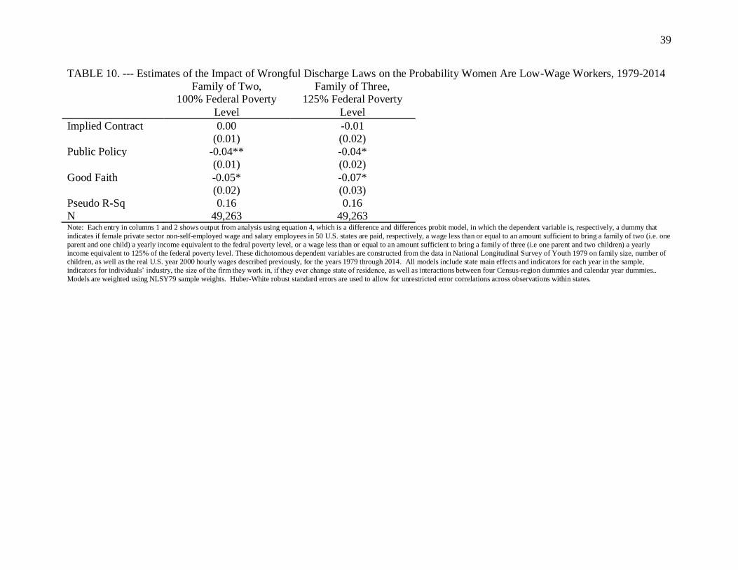
39

TABLE 10. --- Estimates of the Impact of Wrongful Discharge Laws on the Probability Women Are Low-Wage Workers, 1979-2014

Family of Two,

100% Federal Poverty

Level

Family of Three,

125% Federal Poverty

Level

Implied Contract 0.00 -0.01

(0.01) (0.02)

Public Policy -0.04** -0.04*

(0.01) (0.02)

Good Faith -0.05* -0.07*

(0.02) (0.03)

Pseudo R-Sq 0.16 0.16

N 49,263 49,263 Note: Each entry in columns 1 and 2 shows output from analysis using equation 4, which is a difference and differences probit model, in which the dependent variable is, respectively, a dummy that

indicates if female private sector non-self-employed wage and salary employees in 50 U.S. states are paid, respectively, a wage less than or equal to an amount sufficient to bring a family of two (i.e. one

parent and one child) a yearly income equivalent to the fedral poverty level, or a wage less than or equal to an amount sufficient to bring a family of three (i.e one parent and two children) a yearly

income equivalent to 125% of the federal poverty level. These dichotomous dependent variables are constructed from the data in National Longitudinal Survey of Youth 1979 on family size, number of children, as well as the real U.S. year 2000 hourly wages described previously, for the years 1979 through 2014. All models include state main effects and indicators for each year in the sample,

indicators for individuals’ industry, the size of the firm they work in, if they ever change state of residence, as well as interactions between four Census-region dummies and calendar year dummies..

Models are weighted using NLSY79 sample weights. Huber-White robust standard errors are used to allow for unrestricted error correlations across observations within states.

Documents

The Impact of Adoption of Wrongful Discharge Laws on Wages