Univers

ity of

Cap

e Tow

nThe House Dust Microbiota in the

Drakenstein Child Health Study

Menna Duyver

DYVMEN001

SUBMITTED TO THE UNIVERSITY OF CAPE TOWN

In fulfilment of the requirements for the degree

MSc. Medical Microbiology

April 2015

Department of Clinical Laboratory Sciences

Faculty of Health Sciences

UNIVERSITY OF CAPE TOWN

Supervisors: Prof. Mark Nicol

Dr. Lemese Ah Tow

The copyright of this thesis vests in the author. No quotation from it or information derived from it is to be published without full acknowledgement of the source. The thesis is to be used for private study or non-commercial research purposes only.

Published by the University of Cape Town (UCT) in terms of the non-exclusive license granted to UCT by the author.

Unive

rsity

of C

ape

Town

For mom, dad and Hendro

“Somewhere, something incredible is waiting to be known” Carl Sagan

I

Declaration

I, …Menna Duyver……, hereby declare that the work on which this dissertation/thesis is based on

my original work (except where acknowledgements indicate otherwise) and that neither the

whole work nor any part of it has been, is being, or is to be submitted for another degree in this

or any other university.

I empower the university to reproduce for the purpose of research either the whole or any

portion of the contents in any manner whatsoever.

Signature: …………………………………

Date: … 25 May 2015…………….

II

Acknowledgements

I wish to thank my supervisor Prof. Mark Nicol, head of division of Medical Microbiology, University of Cape Town, for providing me with the opportunity to be involved in such a wonderful project. Thank you for your support and guidance throughout my MSc.

I also wish to express my deepest gratitude to my co-supervisor, Dr. Lemese Ah Tow, at the division of Medical Microbiology, University of Cape Town. I am so grateful for the time and patience spent on teaching me new techniques. You are by far one of the best teachers I have had the privilege to work with. Without your guidance and persistent help, this dissertation would not have been possible.

I wish to thank the National Research Foundation, South Africa, as well as the division of Medical Microbiology for personal funding. Without their generous support this would never have been possible.

A big thank you to Mrs Stephanie Mounaud, from Dr William Niermans group at JCVI for preparing the DNA libraries for sequencing. Thank you to JCVI’s sequencing team for performing the Illumina MiSeq run. And thank you to Dr Jyoti Shankar from Dr. William Nierman’s lab for performing the initial bioinformatic analysis.

My sincerest gratitude to A/Prof. Sugnet Lubbe for taking from your personal time to assist me with the quality control & data analysis systems. Thank you for your patience, and for teaching me the joys of R programming.

A big thank you to Ms Anelda van der Walt for assisting me with understanding the concepts involved in chapter 4.

Thank you to Mr Henri Carrara for assisting me with the statistical calculations and advice pertaining to chapter 2.

To Dr. Diane Rip, medical scientist, National Health Laboratory Scientist (Groote Schuur Hospital) thank you for proof reading my dissertation. To the rest of the dream team, Samantha and Veronica, thank you all so much for your support & friendship.

Mom and dad, thank you so much for all your encouragement and financial support. Without you, none of this would have been possible. You ignited a flame in my belly, and fully supported my move from one university to another to make my dream of completing masters in medical microbiology come true.

Grandma even though you are no longer with us, you are a part of this dissertation, thank for all your prayers, you have been with me every step of the way throughout this process.

To my dear Hendro, thank you for being the best husband, and for trying your very best for making this process run as smoothly as possible. Your endless months of cooking and cleaning did not go unnoticed.

To my brother from another mother, Bernard, thank you for all your support. To my wonderful in-laws, thank you for being there for me from the beginning; and thank you for all the take away home-made meals, definitely made this a smoother process.

To my wonderful med micro family, thank you for sharing all the laughs and tears with me. All your support

was so much appreciated.

III

Preface

This dissertation is submitted for the degree of Master in Science (MSc Med) in Medical Microbiology

at the division of Medical Microbiology, Department of Clinical Laboratory Sciences, University of Cape Town,

South Africa. This research project had obtained ethical approval (HREC REF: 743/2013). The parent study was

approved by the Human Research Ethics Committee (HREC) of the Faculty of Health Sciences, University of

Cape Town, South Africa (HREC REF: 401/2009), and approval includes all components of this project. There

were no identifiable significant risks for participants. This study was supported by the Bill and Melinda Gates

Foundation Grant (OPP1017641) and the National Research Foundation (South Africa). The work reported in

this dissertation resulted from a collaborative effort between the J. Craig Venter Institute (JCVI), Maryland,

United States of America, the Departments of Paediatrics and Child Health and Clinical Laboratory Sciences,

the Department of public health and family medicine, and the Department of Statistical Sciences, University of

Cape Town, South Africa.

The aims described in this dissertation were to provide a comprehensive description of the experimental

approaches involved prior to- as well as in generating Illumina MiSeq data for the purpose of characterising the

house dust microbiome at two time points, from the same household. The first chapter presents a detailed

overview of the literature in the context of this project. The second chapter focusses on evaluating ten

commercial nucleic acid extraction protocols on bulk dust samples. Optimisation of dust removal from the

electrostatic cloth (used to collect settled dust), is assessed in the third chapter. All experimental work for

chapter 2 and 3 was fulfilled by the MSc candidate, Mrs Menna Duyver. The fourth chapter focusses on the

experimental and computational approaches used to generate the Illumina MiSeq sequencing data from house

dust samples. The MSc candidate performed the dust removal, nucleic acid extraction as well as quantification

sections included in chapter 4, at the Division of Medical Microbiology, University of Cape Town. The DNA

libraries were prepared by Mrs Stephanie Mounaud, from Dr William Niermans group at JCVI. JCVI’s

sequencing team performed the Illumina MiSeq run. Dr Jyoti Shankar from Dr. William Nierman’s lab

performed the initial bioinformatic analysis. The quality control system was designed by the MSc candidate

and programmed by A/Prof. Sugnet Lubbe from the Department of Statistical Sciences, University of Cape

Town. The fifth chapter deals with analysis of the house dust samples. This chapter used the quality controlled

data that was generated from chapter 4, to study the effect of season on the house dust microbiome, as well

as other external contributors that may influence the house dust microbiome. The data analysis system for

chapter 5 was designed by the MSc candidate and programmed by A/Prof. Sugnet Lubbe from the Department

of Statistical Sciences, University of Cape Town.

The submitted material (which includes experimental procedures, data analyses, results as well as discussion

of the results) is the work of the MSc candidate, unless otherwise stated in the acknowledgments.

IV

Abstract

Introduction: The indoor home environment comprises many niches that are occupied by bacterial

communities. The composition of these bacterial communities may be influenced by numerous factors such as

number of occupants, pets, season and location. Understanding the house dust microbial community is vital to

understanding its’ influence on human respiratory health.

Aims: The aims of the studies described in this MSc dissertation were to: 1) evaluate the performance of ten

commercial nucleic acid extraction kits on dust samples; 2) optimise dust removal from electrostatic dustfall

collectors (EDC); 3) determine the bacterial composition of house dust using 16S rRNA gene sequencing and 4)

determine those factors influencing the bacterial composition of house dust by performing bioinformatic and

data analysis on the sequenced dust samples.

Methods: In order to study the microbial content of house dust, an efficient DNA extraction protocol was

required. Ten commercial nucleic acid purification protocols were evaluated on their ability to efficiently

extract good quality DNA from very low quantities (20 mg) of wet bulk house dust. For the purpose of this

study, EDCs were used to collect settled dust from homes of participants in the Drakenstein Child Health Study

(DCHS). Electrostatic Dustfall Collectors were placed twice within the same household, approximately 6

months apart, spanning two seasons. The Z/R Fungal/Bacterial DNA MicroprepTM

(ZMC) protocol was used to

extract DNA from dust removed from EDCs. The V4 region of the 16S rRNA gene was amplified and sequenced

using the Illumina MiSeq platform to determine the bacterial taxonomic composition of the house dust

samples. A custom python wrapper that meshes a set of tools integrated into a computationally efficient

workflow, known as the YAP pipeline was used to classify 16S rRNA sequences into bacterial taxonomies.

Based on 97% sequence similarity, the pre-processed sequences were assigned to Operational Taxonomic

Units (OTU). R software together with RStudio software was used for all statistical analysis and graphical

representations of the data.

Results and Discussion: Half of the commercial protocols evaluated in this study were able to extract DNA from

20 mg of wet bulk house dust. The ZMC protocol was selected for DNA extractions from dust collected on EDCs

as it was able to consistently yield good quality DNA from as little as 10 mg wet dust. In addition, the DNA

extracted with the ZMC protocol allowed optimal PCR amplification in both end-point and qPCR. Analysis of

the sequencing data indicated an abundance of Actinobacteria, Proteobacteria, and Firmicutes within the

house dust samples. Unsupervised clustering revealed that the clusters between EDC placement one and EDC

placement two within the same household do not cluster together, indicating substantial bacterial variability

within a household over time.This study showed that house dust collected during winter had the highest

bacterial diversity, when compared to house dust collected during any other season. In addition to season,

house type and presence of pets also influenced the composition of the house dust bacterial community.

Increased sample size and additional metadata are required to confirm and extend our findings, and thus

improve our understanding of how external contributors influence the house dust microbiome.

V

Abbreviations

3-OH-FAs – 3-hydrofy fatty acids

A – Autumn

BA – Blood Agar

Bp – Base pairs

CE – Capillary Electrophoresis

CFU – Colony forming Units

DCHS – Drakenstein Child Health Study

ddNTP – dideoxynucleoside triphosphate

DG – Dichloran Glycerol

DGGE – Denaturation Gradient Gel Electrophoresis

DNA – Deoxyribose Nucleic Acid

EDC – Electrostatic dustfall collector

EMP – Earth Microbiome Project

EPS – Extracellular polysaccharides

EPS-ASP-PEN – Aspergillus & Penecillium species

EtBr – Ethidium Bromide

EtOH – Ethanol

FD – FastDNATM

Spin kit for soil

FISH – Fluorescent in situ hybridisation

F – Flat

GE – GenElute Plant Genomic DNA Miniprep Kit

GLM – Generalise Linear Models

GLMM – Generalised Linear Mixed Models

H – House

Indel – Insertion/ deletion

ITS – Internal Transcribed Spacer

LAL – Limulus Amebocyte Lysate

LPS – Lipopolysaccharide

MAE – Maltose Extract Agar

MDS – Multidimensional Scaling plot

MSQPCR – Mould specific qPCR

NS – NucleoSpin® kit for Soil

NA – Nucleic acid

NAE – Nucleic Acid Extraction

NCTC – National Collection of Type Cultures

NGS – Next Generation Sequencing

NTC – No template control

O – Other

OTU – Operational Taxonomic Unit

P – PowerSoil® DNA Isolation kit

VI

PBS – Phosphate Buffered saline

PC – Positive Control

PCR – Polymerase Chain Reaction

PFW – Pyrogen Free water

PS – pyrosequencing

PS – Pyrosequencing

QCL – Kinetic chromogenic LAL

QIIME – Quantitative Insights Into Microbial Ecology

qPCR – Real-time/quantitative Polymerase Chain Reaction

QS – Qiasymphony (DSP Virus/bacteria midi kit)

RNA – Ribose Nucleic Acid

rRNA – ribosomal RNA

SA – South Africa

S – Shack

SM – SoilMasterTM

DNA extraction kit

Sm – Summer

SNPs – Single nucleotide polymorphisms

Sp – Spring

SSCP – Single Strand Confirmation Polymorphism

TLR – Toll Like Receptors

T-RFLP – Terminal Restriction Fragment Length Polymorphism

TSA – Tryptic Soy agar

UC – UltraClean® Microbial DNA Isolation

UCF – UltraClean® Fecal DNA isolation kit

UV – Ultraviolet

UVGI – Ultraviolet Germicidal Irradiation

VOCs – Volatile compounds

W – Winter

YAP – Yet Another Pipeline

ZMC – Z/R Fungal/Bacterial DNA MicroPrep TM

ZMN – Z/R Fungal/Bacterial DNA MiniPrep TM

VII

Glossary of terms

16S rRNA –the smaller RNA component of the prokaryotic ribosome which is used as the most common taxanomic marker

for microbial communities (Morgan & Huttenhower 2012).

Alpha diversity (α-diveristy) – taxonomic diversity within a sample (Morgan & Huttenhower 2012).

Atopy – the predisposition towards developing certain allergic hypersensitivity reactions (such as asthma, eczema etc).

Beta diversity (β-diversity) – taxonomic diversity between a sample (Morgan & Huttenhower 2012).

Bridge PCR – PCR that occurs between primers that are bound to a surface (Glenn 2011).

Bulk Dust – Dust collected from several vacuum cleaner bags to create one mixed, homogenous sample

Chimeric sequence – During the PCR amplification process, some of the amplified sequences can be produced from

multiple parent sequences, generating sequences known as chimeras. This results from a premature

dissociation of an amplicon from its template, therefore acting as a primer to another and different sequence

(Tyler et al., 2014; Navas-Molina et al., 2013).

Cluster – groups of similar sequences (Tyler et al., 2014).

Conventional PCR – used to amplify a single copy (or few copies) of a piece of DNA, generating thousands of copies of a

particular DNA sequence

Coverage – Number of sequences obtained per sample in a sequencing run (Tyler et al., 2014).

Demultiplexing – is a process whereby the barcodes that are tagged on the reads are identified and these reads that go

with the barcodes are packaged into FASTQ files.

Diversity – An estimate of abundance and species richness to measure the microbial variability either within a sample (α-

diversity) or between samples (β- diversity) (Tyler et al., 2014).

DNA barcode – a short DNA sequence that is unique to each sample (Navas-Molina et al., 2013).

Dynamic trim – a read trimmer that individually crops each read to its longest contiguous segment for which quality scores

are greater than a user-supplied quality cut off.

Evenness – In a sample/ community, the measure of homogeneity of abundance (Gotelli & Colwell 2009)

Flow cell – A single-use sequencing slide/chip/plate used by Illumina sequencers (Glenn 2011).

Hygiene Hypothesis – this hypothesis states that a lack of exposure to symbiotic and or infectious organisms, as well as

parasites, during early childhood could increase the susceptibility of a child towards allergic diseases

(Strachan 1989).

Limit of detection – lowest quantity of a substance that can be distinguished (Morgan & Huttenhower 2012).

Mean Quality score – total sum of Q scores of clusters that passed filtering divided by the total yield of the clusters that

had passed filtering

Metagenomics – the study of uncultured microbial communities, which typically rely on high throughput data and

bioinformatics analysis (Morgan & Huttenhower 2012).

VIII

Microbiome – the biomolecules and total microbial community within a defined environment (Morgan & Huttenhower

2012).

Microbiota – the total collection of microbial organisms present within a community (Morgan & Huttenhower 2012).

Operational Taxanomic Unit (OTU) – Sequences that are clustered into groups at a prespecified similarity. The

representative sequences present within OTUs can be assigned to a taxonomy based on the comparison of

sequences with a known reference database (Tyler et al., 2014).

Paired-end reads – during the sequencing process, when templates are sequenced first from one end, and then from the

other end. This allows for the generation of extended reads, which almost doubles the maximum sequencing

length available using a given sequencing technology (Glenn 2011; Tyler et al., 2014).

Phred score – a quality score for each nucleotide that is generate (Navas-Molina et al., 2013).

Q score – Quality score also known as the Phred score

Quality threshold – DNA sequences from each end of DNA templates (Navas-Molina et al., 2013).

RDP – Used for taxonomy assignment

Read Length – is the pair length of sequences that result from a sequencing run (Tyler et al., 2014).

Real time PCR – based on the PCR, it is also used to amplify a target DNA molecular, however it detects or quantifies this

target DNA molecule as well.

Relative Abundance – is the quantitative measure of OTUs, number of organisms or sequences detected in a sample. This

can be calculated by dividing the number of individuals within a group by the total number of sequences

present within a sample (Tyler et al., 2014).

Richness – Within a specific sample, it is the number of unique organisms detected (Tyler et al., 2014).

Species richness – The number of species within a community (Colwell 2009)

SYBR green – is a dye that is used a nucleic acid stain in molecular biology, used in qPCR.

Taxa – groups of populations/organisms that seen by taxonomists to form a unit

Universal primer – PCR primer that has the capability of binding to sequences from many different organisms. These

primers bind to a genetic regions of high similarity therefore ensuring that a broad spectrum of organisms are

represented (Tyler et al., 2014).

V4 region –Variable 4 region of the 16S rRNA gene

YAP – 16S bioinformatics workflow for preliminary data processing of MiSeq as well as 454 reads.

IX

Table of Contents Declaration ............................................................................................................................................... I

Acknowledgements ................................................................................................................................. II

Preface ................................................................................................................................................... III

Abstract .................................................................................................................................................. IV

Abbreviations .......................................................................................................................................... V

Glossary of terms .................................................................................................................................. VII

List of Tables ........................................................................................................................................ XIV

List of Figures ........................................................................................................................................ XV

General Introduction............................................................................................................................... 1

CHAPTER 1: Literature Review: The House Dust Microbiome ................................................................ 2

1.1. House dust .............................................................................................................................. 3

1.1.1. Search Strategy ............................................................................................................... 4

1.1.2. Background to house dust .............................................................................................. 4

1.1.3. Associations of house dust bacteria to respiratory health and the hygiene hypothesis 5

1.1.4. Microorganisms present within house dust ................................................................... 7

1.1.4.1. Bacteria ................................................................................................................... 7

1.1.4.2. Fungi ........................................................................................................................ 7

1.1.4.3. Viruses ..................................................................................................................... 8

1.1.5. External contributors to house dust ............................................................................... 8

1.1.5.1. Occupants ............................................................................................................... 8

1.1.5.2. Pets ........................................................................................................................ 10

1.1.6. Sampling methods for house dust ................................................................................ 11

1.1.7. Processing of indoor/house dust .................................................................................. 12

1.1.8. Techniques used to study house dust ........................................................................... 13

1.1.8.1. Culture dependent techniques ............................................................................. 14

1.1.8.1.1. Bacteria .............................................................................................................. 14

1.1.8.1.2. Fungi ................................................................................................................... 16

1.1.8.2. Biochemical techniques used to study the bacterial microbiome in house dust . 16

1.1.8.2.1. Endotoxin ........................................................................................................... 16

1.1.8.2.2. Muramic Acid .................................................................................................... 18

1.1.8.3. Biochemical techniques used to study the fungal microbiota in house dust ....... 19

1.2. Molecular Biology Techniques .............................................................................................. 20

1.2.1. The history of nucleic acid extraction ........................................................................... 20

1.2.1.1. DNA extraction protocols used for isolation of DNA from indoor dust samples .. 22

1.2.2. Molecular-based techniques used to study the microbial composition of dust .......... 23

1.2.2.1. Molecular techniques used to study house dust bacteria .................................... 24

1.2.2.2. Molecular techniques used to study house dust fungi ......................................... 25

1.3. Microbiome studies of house dust ....................................................................................... 26

X

1.3.1. History behind microbiome studies .............................................................................. 26

1.3.2. Microbiome Sequencing ............................................................................................... 27

1.3.3. Sequencing Technologies .............................................................................................. 29

1.3.4. Sequencing Steps .......................................................................................................... 31

1.3.4.1. Bioinformatic Pipeline ........................................................................................... 31

1.3.5. Sequencing to study the bacteria present within dust samples ................................... 34

1.3.6. Sequencing to study the Fungi present within dust samples ....................................... 35

1.4. Factors affecting the house dust microflora ......................................................................... 36

1.4.1. Type of indoor environment ......................................................................................... 36

1.4.2. Season ........................................................................................................................... 37

1.5. Study Objectives ................................................................................................................... 39

CHAPTER 2: Evaluation of Commercial Nucleic Acid Purification Protocols for the Extraction of DNA from Household Dust ............................................................................................................................ 40

2.1. Aims....................................................................................................................................... 41

2.2. Methods ................................................................................................................................ 41

2.2.1. Dust sample collection .................................................................................................. 42

2.2.2. DNA extraction from bulk house dust .......................................................................... 42

2.2.2.1. DNA extraction and optimisation.......................................................................... 43

2.2.2.1.1. Sample lysis ....................................................................................................... 43

2.2.2.1.2. DNA elution volumes ........................................................................................ 43

2.2.2.2. Modifications to DNA extraction methods ........................................................... 44

2.2.3. Determination of DNA quality and integrity ................................................................. 45

2.2.4. 16S rRNA gene end–point PCR ...................................................................................... 45

2.2.4.1. PCR positive control .............................................................................................. 46

2.2.4.2. 16S rRNA PCR optimisations ................................................................................. 46

2.2.4.3. Optimised 16S rRNA PCR protocol ........................................................................ 46

2.2.5. 16S rRNA gene qPCR ..................................................................................................... 47

2.2.5.1. 16S rRNA qPCR optimisations ............................................................................... 47

2.2.5.2. Optimised 16S rRNA qPCR protocol ...................................................................... 47

2.2.6. Statistical analysis ......................................................................................................... 47

2.3. Results ................................................................................................................................... 48

2.3.1. Nucleic acid quality and integrity .................................................................................. 48

2.3.1.1. Manufacturer’s recommendations ....................................................................... 48

2.3.1.2. Modifications to DNA extraction methods ........................................................... 49

2.3.1.2.1. Decreasing amount of starting wet weight of dust .......................................... 49

2.3.1.2.2. Inclusion of a Uniform Mechanical Lysis step ................................................... 52

2.3.1.3. Comparison of the 5 best protocols using 50 mg wet dust .................................. 54

2.3.2. 16S rRNA gene end-point PCR ...................................................................................... 56

2.3.2.1. Positive control ..................................................................................................... 56

2.3.2.2. 16S rRNA PCR protocol ......................................................................................... 57

XI

2.3.2.3. 16S rRNA PCR optimisation tests .......................................................................... 58

2.3.3. 16S rRNA gene SYBRgreen qPCR ................................................................................... 58

2.3.3.1. 16S rRNA qPCR optimisation tests ........................................................................ 58

2.3.3.2. 16S rRNA qPCR optimised protocol ...................................................................... 59

2.4. Discussion .............................................................................................................................. 60

2.5. Conclusion ............................................................................................................................. 66

CHAPTER 3: Optimization of Dust Sample Collection and Pre-analytical Processing ........................... 67

3.1. Aims....................................................................................................................................... 68

3.2. Methods ................................................................................................................................ 68

3.2.1. Preparation and sterilization of Electrostatic Dust Collectors (EDC’s) .......................... 68

3.2.2. Assessment of the EDC sterilisation process ................................................................ 69

3.2.3. Optimisation of dust removal from EDC’s .................................................................... 71

3.2.4. DNA extraction .............................................................................................................. 73

3.2.4.1. Optimization of DNA extraction using bulk dust .................................................. 73

3.2.4.2. DNA extraction from dust removed from the EDC’s ............................................. 75

3.2.5. 16S rRNA end-point PCR optimisation using DNA extracted from bulk dust ............... 75

3.3. Results ................................................................................................................................... 76

3.3.1. Assessment of the EDC sterilisation process ................................................................ 76

3.3.2. Dust removal and DNA quantification from EDC’s ....................................................... 76

3.3.3. Optimisation of the ZMC DNA extraction protocol using bulk dust ............................. 77

3.3.4. 16S rRNA end-point PCR ............................................................................................... 78

3.3.4.1. 16S rRNA end-point PCR optimisations on DNA extracted from bulk dust .......... 78

3.3.4.2. Optimised 16S rRNA end-point PCR using DNA extracted from EDC’s ................. 79

3.4. Discussion .............................................................................................................................. 79

3.5. Conclusion ............................................................................................................................. 82

CHAPTER 4: Next Generation Sequencing of Household Dust Samples: A Pilot Study ........................ 83

4.1. Aims....................................................................................................................................... 84

4.2. Methods ................................................................................................................................ 85

4.2.1. Study Design .................................................................................................................. 85

4.2.2. Study Population ........................................................................................................... 86

4.2.3. Sample size and selection criteria ................................................................................. 86

4.2.4. Dust collection and DNA extraction .............................................................................. 86

4.2.4.1. Dust removal and DNA extraction ........................................................................ 87

4.2.4.1.1. DNA quantification ............................................................................................ 88

4.2.5. 16S rRNA amplicon Library preparation ....................................................................... 88

4.2.6. Running of the 16S rRNA YAP pipeline ......................................................................... 89

4.2.7. Statistical analysis ......................................................................................................... 91

4.3. Results ................................................................................................................................... 91

4.3.1. Dust removal and DNA extraction ................................................................................ 91

XII

4.3.2. Summary statistics on the data metrics obtained from the Illumina MiSeq sequencer software and the 16S YAP workflow for all sampling groups ....................................................... 93

4.3.2.1. Summary statistics on the data metrics obtained from the Illumina MiSeq sequencer software and the 16S YAP workflow for all sampling groups, based on season .... 94

4.3.2.2. Summary statistics on the data metrics obtained from the Illumina MiSeq sequencer software and the 16S YAP workflow for all sampling groups, based on placement... ............................................................................................................................... 95

4.3.2.3. Summary statistics –Rarefaction curves ............................................................... 95

4.3.2.4. Summary statistics –Reproducibility between duplicate sequenced samples ..... 96

4.3.2.5. Summary statistics for the Sterile EDCs and Non template control .................... 96

4.4. Discussion .............................................................................................................................. 97

4.5. Conclusion ........................................................................................................................... 100

CHAPTER 5: Pilot Study Data Analysis ................................................................................................. 101

5.1. Aims..................................................................................................................................... 102

5.2. Statistical Analysis methods ................................................................................................ 102

5.2.1. Accounting for OTUs found in the sterile EDCs .......................................................... 102

5.2.2. Measuring Diversity .................................................................................................... 103

5.2.2.1. Shannon diversity ................................................................................................ 103

5.2.2.2. Barplots ............................................................................................................... 104

5.2.2.2.1. Bray-Curtis Dissimilarity Index ........................................................................ 104

5.2.2.2.2. Complete linkage of hierarchical clustering .................................................... 105

5.2.2.2.3. Multidimensional scaling plots ....................................................................... 105

5.2.2.3. Biplots ................................................................................................................. 106

5.2.2.4. Generalised Linear Mixed Models ...................................................................... 106

5.3. Results ................................................................................................................................. 107

5.3.1. Genera present in the no-template control and sterile EDC controls ........................ 108

5.3.2. Accounting for the OTUs present in the sterile EDCs ................................................. 112

5.3.3. House dust microbiome .............................................................................................. 113

5.3.3.1. House dust microbiome and external contributing factors ................................ 120

5.3.3.1.1. House dust microbiome across the seasons .................................................... 120

5.3.3.1.2. House dust microbiome and type of home .................................................... 126

5.3.3.1.3. House dust microbiome and pets ................................................................... 130

5.3.3.1.4. House dust microbiome and human occupancy ............................................ 132

5.3.3.1.5. House dust microbiome and size of home ..................................................... 133

5.3.3.1.6. House dust microbiome and Windows ........................................................... 133

5.3.3.1.7. House dust microbiome and region ................................................................ 134

5.4. Discussion ............................................................................................................................ 135

5.6. Conclusion ........................................................................................................................... 140

Chapter 6: General Discussion ............................................................................................................ 141

Conclusion ........................................................................................................................................... 146

Literature Cited ................................................................................................................................... 147

XIII

Appendices .......................................................................................................................................... 164

Appendix A ...................................................................................................................................... 165

Appendix B ...................................................................................................................................... 166

Appendix C ...................................................................................................................................... 167

Appendix D ...................................................................................................................................... 169

Appendix E ...................................................................................................................................... 170

Appendix F ...................................................................................................................................... 171

Appendix G ...................................................................................................................................... 178

Appendix H ...................................................................................................................................... 180

Appendix I ....................................................................................................................................... 185

XIV

List of Tables

Table 1.1: Types of culture media used for the isolation of bacterial species from indoor dust samples.

Table 1.2: Molecular based techniques used on dust samples.

Table 1.3: Comparison between NGS sequencers.

Table 2.1: Summary of the 10 commercial NA extraction protocols that were assessed in this study.

Table 2.2: Manufacturer’s recommendations for all NA extraction protocols used in this study.

Table 2.3: Comparison between the median DNA concentration and purity, by protocol and weight between the manufacturer’s recommendations and the modified protocol.

Table 2.4: Comparison between the 5 best protocols, in terms of purity and concentration at 50 mg starting wet weight.

Table 3.1: Bacterial and fungal growth from treated electrostatic cloths.

Table 3.2: Starting wet weight of dust and total DNA obtained for the 5 EDC’s.

Table 3.3: Comparison of the total DNA (ng) obtained from 10 mg wet dust (in duplicate) using the adapted ZMC DNA extraction methods.

Table 4.1: Summary of the number and sample type that were sequenced.

Table 4.2: Total Number of reads obtained per sequencing step, with the average number of reads per sample per output step.

Table 5.1: Table indicating the different taxonomic levels of the 13 genera that were identified in the sterile

samples only.

Table 5.2: Table indicating the different taxonomic levels of the 20 genera that had scaled deviations of more than 0.5, and needed to be corrected for.

XV

List of Figures

Figure 1.1: Diagrammatic summary of literature review.

Figure 1.2: Structures of a) Lipopolysaccharide, b) Muramic acid.

Figure 1.3: Structure of β-(13)-glucans.

Figure 1.4: A Schematic representation of the 16S rRNA gene.

Figure 1.5: A schematic representation of the general overview of a 16S metagenomics bioinformatics pipeline.

Figure 2.1: Diagram depicting the flow of events in which the 10 commercial Nucleic acid extraction protocols

were assessed.

Figure 2.2: A) Bar graph representing the DNA concentrations & purities of the 10 protocols performed according to the manufacturer’s specifications, at each of their lowest recommended starting wet weights.

Figure 2.3: Representative agarose gels depicting genomic DNA extracted with A) ZMN B) NS & C) UCF NA extraction protocols.

Figure 2.4: Bar graphs representing DNA concentrations and purities of the protocols performed according to the manufacturer’s recommendations at 100 mg, 50 mg and 20 mg, respectively.

Figure 2.5: Representative agarose gel image of NA extracted using the P protocol at the recommended starting weight of 250 mg.

Figure 2.6: Bar graphs representing the DNA concentrations & purities of the 10 protocols performed according to the manufacturer’s recommendations, and according to the uniform mechanical lysis step at their lowest recommended starting wet weights.

Figure 2.7: Box plots representing DNA concentrations & purities of the DNA extracted from 50 mg starting wet weight of dust using the 5 best protocols.

Figure 2.8: 16S rRNA PCR amplicons of the positive control, S. aureus, at decreasing template amounts.

Figure 2.9: Representative agarose gel depicting 16S rRNA PCR amplicons using DNA extracted from 50 mg wet dust.

Figure 2.10: qPCR results of 1 PC, and 3 NTC’s.

Figure 2.11: qPCR results comparing the 2 SYBR Green master mixes.

Figure 2.12: Final qPCR results of the 5 best protocols.

Figure 3.1: Representative image of an EDC.

Figure 3.2: EDC UV sterilisation.

Figure 3.3: Assessment of the EDC sterilisation process.

Figure 3.4: Flow diagram depicting the removal of dust from the electrostatic cloth.

Figure 3.5: Flow diagrams depicting the various optimisation steps that were carried out for the ZMC protocol.

Figure 3.6: Agarose gel depicting the 3 different master mixes assessed.

Figure 3.7: Agarose gel depicting the PCR amplicons obtained using the KAPA master mix.

Figure 4.1: Flow diagram depicting the breakdown of events for this experimental chapter.

Figure 4.2: Map of South Africa.

Figure 4.3: Flow diagram depicting the chain of events from dust removal to DNA elution.

Figure 4.4: Flow diagram representing the sequence of events for 16S rRNA amplicon preparation.

XVI

Figure 4.5: Summary of the bioinformatics steps included in the YAP pipeline.

Figure 4.6: Dust quantities obtained (mg) per EDC.

Figure 4.7: DNA concentrations (ng/µl) obtained for each of the 120 EDCs.

Figure 4.8: Box plot representing the DNA yield (ng/µl), according to season.

Figure 4.9: Box plot representing the DNA yield (ng/µl), according to placement.

Figure 4.10: Notched box plots, representing the Mean Quality Scores according to seasons.

Figure 4.11: Notched box plots, representing the Mean quality score according to placements.

Figure 4.12: Rarefaction curves of high throughput sequencing of the V4 region of the 16S rRNA gene.

Figure 4.13: Regression line indicating the reproducibility between the duplicate samples.

Figure 5.1: Pie chart indicating A) the proportion of genera identified in the sterile EDCs and B) the same genera identified in the sterile EDCs and in the dust samples.

Figure 5.2: Barplot representing the OTU counts of genera in the sterile EDCs and dust samples.

Figure 5.3: Colour key for Figure 5.2.

Figure 5.4: Box plots representing the 20 genera with scaled deviations >0.5. A) Before and B) after the correction was made.

Figure 5.5: Representation of all the taxa, at class level across the 120 dust samples.

Figure 5.6: Barplot representing the lower abundant taxa (<0.5) at class level across all 120 dust samples.

Figure 5.7: Multidimensional scaling plot indicating A) the clusters that correspond to all the taxa present in dust samples, and B) the clusters that correspond to the lower abundant taxa only.

Figure 5.8: Higher abundant taxa, at class level, across the 120 dust samples (separated into their pairs).

Figure 5.9: Notched box plots based on the Shannon diversity index, comparing the diversities between the EDC placements.

Figure 5.10: Biplot analysis used to compare the difference in the compositional data between placement 1 and placement 2.

Figure 5.11: Notched box plots based on the Shannon diversity index. Comparison of the diversities between the seasons.

Figure 5.12: Barplot representing the overall relative distribution of the most abundant bacterial phyla across the different seasons.

Figure 5.13: Plots representing the different taxa significantly influenced by season. Taxa with the highest rate ratios for summer are shown.

Figure 5.14: Plots representing the different taxa significantly influenced by season. Taxa with the highest rate ratios for spring are shown.

Figure 5.15: Plots representing the different taxa significantly influenced by season. Taxa with the highest rate ratios for Winter are shown.

Figure 5.16: Plots representing the different taxa significantly influenced by season. Taxa with the highest rate ratios for Autumn are shown.

Figure 5.17: Box plots representing Shannon diversity indices between the different types of households.

Figure 5.18: Barplots representing the overall relative abundance of the bacteria at phylum level in different types of dwellings.

Figure 5.19: Plots representing the different taxa significantly influenced by house type. Taxa with the highest rate ratios in house type “other” are shown.

Figure 5.20: Plots representing the different taxa significantly influenced by house type. Taxa with the highest rate ratios in house type “shack” are shown.

Figure 5.21: Plots representing the different taxa significantly influenced by house type. Taxa with the highest rate ratios in house type “flat” are shown.

XVII

Figure 5.22: Plots representing the different taxa significantly influenced by house type. Taxa with the highest rate ratios in house type “house” are shown.

Figure 5.23: Box plots representing Shannon diversity indices between A) homes with and without pets. B) Homes between different numbers of pets

Figure 5.24: Barplots representing the overall relative abundance of the bacteria at phylum level between the households with and without pets

Figure 5.25: Plots representing the different taxa significantly influenced by the presence of pets. These taxa are most abundant in homes with pets

Figure 5.26: Box plots based on the Shannon diversity indices, representing the diversity obtained in each household based on the number of occupants

Figure 5.27: Box plots representing Shannon diversity indices between the number of rooms within a household

Figure 5.28: Box plots representing Shannon diversity indices between the households that had windows open or closed during placement of the EDCs

Figure 5.29: Box plots representing Shannon diversity indices between the two different regions of placement

Figure 5.30: The overall relative abundance of the bacterial phyla between the two different regions, Mbekweni and TC Newman

1

General Introduction

With increasing urbanisation, individuals tend to spend most of their time indoors. Some

studies have estimated that individuals spend at least 90% of their time indoors (Custovic et al.,

1994; Hoppe & Martinac 1998). Babies are born in a hospital, are raised in either homes or

apartments, placed in day care when they get older, go to school, work in office buildings, and then

move into old age homes or retirement villages. In these internal environments, humans are

surrounded by a variety of living organisms, such as fungi, bacteria, plants and arthropods (Dunn et

al., 2013). The impact of these organisms on our overall well-being and health is understudied. This

is most certainly the case for fungi and bacteria that reside within our homes. These taxa can either

have a positive or adverse effect on human respiratory health (Hoppe & Martinac 1998; Shen 2008;

Flores et al., 2011; Hewitt et al., 2013).

Little is known about the microbial communities present in homes, and how their structure changes

within a home, or between different households within the same location (Kembel et al., 2012a).

However, this has become a growing topic of interest (Dunn et al., 2013; Lax et al., 2014; Meadow et

al., 2014a; Meadow et al., 2014b)

Whilst culture-dependent techniques show that micro-organisms are ubiquitous within the indoor

environment, culture independent techniques have shown that the microbial diversity present

within the indoor environment is more substantial than previously noted (Dawson et al., 2007;

Fujimura et al., 2014). Biochemical techniques can reveal the relative abundance of the bacterial and

fungal load; however biochemical techniques are not useful for the identification of the bacteria

present within a sample. Hence there is growing interest towards characterising the microbial

composition in the environment (Karvonen et al., 2014). Molecular techniques, more specifically,

Next Generation Sequencing (NGS) can be used for the identification of the bacteria present within a

sample. Hence, the question would no longer be “does a home present as a habitat to microbial

communities” but rather “how many and what kind of micro-organisms are present?”

The purpose of this MSc dissertation is to characterise the house dust microbiome, as well as to

study the influence that season and other contributing factors may have on the house dust

microbiome. This study forms part of the Drakenstein Child Health Study. This association will be

studied with the use of Next Generation Illumina Sequencing, targeting the 16S rRNA gene.

2

CHAPTER 1

Literature Review: The House Dust Microbiome

3

Chapter 1: The House Dust Microbiome 1.1. House dust

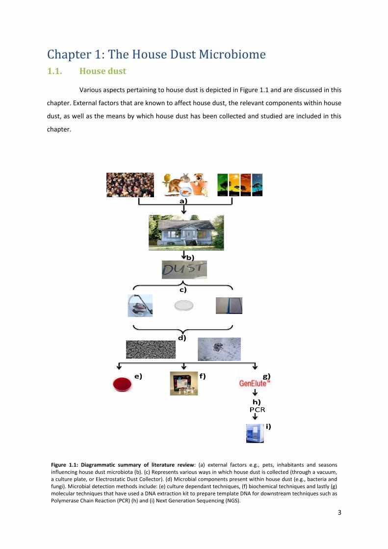
Various aspects pertaining to house dust is depicted in Figure 1.1 and are discussed in this

chapter. External factors that are known to affect house dust, the relevant components within house

dust, as well as the means by which house dust has been collected and studied are included in this

chapter.

Figure 1.1: Diagrammatic summary of literature review: (a) external factors e.g., pets, inhabitants and seasons influencing house dust microbiota (b). (c) Represents various ways in which house dust is collected (through a vacuum, a culture plate, or Electrostatic Dust Collector). (d) Microbial components present within house dust (e.g., bacteria and fungi). Microbial detection methods include: (e) culture dependant techniques, (f) biochemical techniques and lastly (g) molecular techniques that have used a DNA extraction kit to prepare template DNA for downstream techniques such as Polymerase Chain Reaction (PCR) (h) and (i) Next Generation Sequencing (NGS).

4

1.1.1. Search Strategy

The studies that were included for this MSc were published between 1887 and 2015.

Language restrictions were placed on English and German papers only, and the databases used

include: Pubmed, Google Scholar and Web of Science. Key words include: “dust”, “house dust”,

“indoor dust”, “sequencing” “Next Generation Sequencing”, “bacteria”, “fung*”, “culture”,

“biochemical” and “Molecular”.

1.1.2. Background to house dust

“Settled dust” and “house dust” are both terms most commonly used to describe

particulate matter collected on horizontal surfaces (Macher 2001), which is considered by the

Institute of Medicine (2004) as an integrated sample of particles that once were airborne. A

relationship exists between the amount of inhaled allergen that was airborne and the allergens

present within settled dust (Macher 2001). Settled dust is considered to be a more appropriate

representation of airborne dust. In contrast, dust samples collected from mattresses and floors

contain both airborne dust as well as particulate matter that originated from the occupants

themselves (such as skin flakes or hair), or particulate matter tracked into the house via shoes, or

clothing (Korthals et al., 2008(b); Normand et al., 2009; Kelley & Gilbert 2013; Lax et al., 2014).

Therefore, reasons for wanting to study dust instead of household air is that dust samples are

inexpensive and easier to collect (Macher 2001).

House dust commonly consists of, but is not limited to, a multifaceted mixture of skin flakes, insect

parts, animal and human hair, particles of plants, soil, atmospheric dust, material from both

bacterial and fungal species (living and dead) (Macher 2001), dust mites and allergens (Rintala et al.,

2012). In addition, substances that are known to add to the allergenicity of dust, such as fragments

and excreta from arthropods (cockroaches, house dust mites, arachnids and other insects), as well as

urine from wild and domestic animals (e.g., rodents, birds, cats and dogs), saliva and dander

(Macher 2001) can all form part of dust samples.

The development of microbial communities present within indoor dust is attributed to the

deposition from the air. The air within households is in continuous movement due to human

activities and ventilation. Smaller microbial particles present within house dust have a tendency to

mix more efficiently within the room space, and stay airborne for longer periods in comparison to

5

their bigger counterparts (Oberoi et al., 2010). Hence, inhalation exposure is most likely due to the

smaller particles that would remain airborne for increased periods (Macher 2001).

Researchers have studied the micro-organisms present within house dust to gain an insight into the

association between indoor contaminants and human exposure. As early as 1887, Carnelley and

associates studied household dust, focusing on carbonic acid, micro-organisms and organic matter in

schools and dwellings (Carnelley et al., 1887). Subsequent studies were conducted in the 1940s and

1950s to study fungal levels present within house dust (Morrow & Lowe 1943). Later studies then

ensued where house dust was investigated within the context of health, where the agents within

house dust were seen as either harmful or beneficial towards an individual’s health and well-being

(Ege et al., 2011). This is explained as the hygiene hypothesis.

1.1.3. Associations of house dust bacteria to respiratory health and the hygiene

hypothesis

In past years, attention has centred around the role that aeroallergens play in both the

development and the severity of asthma (Ren et al., 1999).

In developed countries, wheezing is known to affect approximately one-third of infants within the

first year of life (Landau 2002). Wheezing is due to obstruction of the lower airways and is a non-

specific symptom (Landau 2002). It is defined as a high pitched sound, which is continuous and

which emits from the chest during expiration (Elphick 2001). Wheezing during childhood and infancy

is a symptom associated with a number of illnesses, such as asthma (Martinez et al., 1995; Rusconi

et al., 1999) and acute respiratory tract infections.

Recurrent wheezing is characteristic of asthma (Rusconi et al., 1999). Most children that have

asthma are known to present with the symptom of wheezing, however, not all children that wheeze

have asthma (Rusconi et al., 1999). Asthma is a condition that results from complex interactions

between multiple environmental and genetic influences (Weiss 2012). Numerous risk factors for

asthma have been identified (Weiss 2012). The best studied risk factors include exposure to

cigarette smoke (both antenatally and postnatally), gender, atopy, allergens, infections, obesity as

well as perinatal factors (Etzel 2003; Subbarao et al., 2009; Weiss 2012).

6

Within the last few decades an increase in the global prevalence of asthma and allergy has been

observed (Asher et al., 1998). This is increasingly apparent within the developed world, however

similar increases have been observed in the low-income countries as well (Pearce & Douwes 2006).

The reasons for the increase are not clear. These changes are unlikely due to genetic changes,

because the time frame involved is too short (Brooks et al., 2013). A reduction in the prevalence of

infectious diseases is in strong contrast with the increase of allergies. This association has led to the

development of the hygiene hypothesis, which states that asthma and allergy epidemics are due to

the decreased exposure of individuals to both infectious and non-infectious micro-organisms

(Strachan 1997; Eder et al., 2006).

The hygiene hypothesis was initiated by evidence that showed that overcrowding, large family sizes

and less hygienic conditions are associated with a decrease in the prevalence of asthma, atopy,

eczema and hay fever (Strachan 1989; Strachan 1997; Asher et al., 1998; Krämer et al., 1999; Ball et

al., 2000). The increased exposures of individuals to micro-organisms and/or to microbial

components, as well as an increase in infections in the settings described above have all been

proposed to explain these findings (Martinez et al., 1995).

Holt et al., (1995; 1997) and Yabuhara et al., (1997) have described how the immune response is

primed when exposed to micro-organisms. It is proposed that when a child grows up within an

environment that is rich in micro-organisms this would result in the child developing a balanced T

helper (Th)2 and (Th)1 response (Holt et al., 1995; Holt et al., 1997). In contrast, a child growing up in

a more ‘hygienic’ environment (which contains fewer and less diverse micro-organisms) develops an

immune response that is skewed towards the Th2 direction (Eder & von Mutius 2004; Kozyrskyj et

al., 2007), which is associated with asthma.

A good example of the hygiene hypothesis can be seen in the case of children from farming

communities, who are exposed to a vast number and diversity of micro-organisms. These children

have a lower prevalence of asthma and atopy in comparison to children growing up in urban

communities (Brooks et al., 2013)

7

A systematic review published by Mendy et al., (2011), showed that bacterial endotoxins may have a

protective effect for the development of asthma. Endotoxins are indicative of the Gram-negative

species and are therefore not a true representation of the bacterial diversity (Rylander 2002).

1.1.4. Microorganisms present within house dust

1.1.4.1. Bacteria

Dust samples contain both living and dead bacteria, as well as fragments of degraded

cells, spores and endospores. The size of bacterial cells are smaller than fungal cells, with their sizes

ranging up to 1 µm (Reponen et al., 1998).

Gram staining classifies bacteria into two major groups: Gram-positive and Gram-negative (Gram

1884), based on their cell wall structures. Lipopolysaccharide (also termed endotoxin) (Figure 1.2A),

are a major cell wall component of Gram-negative bacteria (Adhikari et al., 2014) whereas, muramic

acid are the major cell wall component of Gram-positive bacteria (Adhikari et al., 2014) (Figure 1.2B).

Both endotoxin and muramic acids are biochemical markers that can be used to measure overall

bacterial presence and bacterial biomass within a sample (Täubel et al., 2009).

1.1.4.2. Fungi

The fungal components in house dust may include fungal spores, where their size and

shape vary from large oblong shaped conidia of approximately 50 µm in size (e.g., Alternaria &

Helminthosporium), to small round or ovoid shaped conidia of 2 - 5 µm in size (e.g., Aspergillus,

Penicillium). Other fungal components found within house dust may also include fruiting bodies,

sclerotia, lichen, sporadia, hyphae, spore clumps and fragments of spores (Green et al., 2006).

The indoor environment is home to many fungal taxa. Fungal fragments and spores carry

components such as ergosterol and β-(13)-glucan, which are common to all fungi. Fungal research

has primarily focussed on detecting surface growth (especially in the context of water damaged

buildings) (Adams et al., 2014). β-(13)-glucan and ergosterol are used as biochemical markers to

measure fungal exposure within the indoor environment (Rylander et al., 1999; Douwes et al., 2000;

Hyvärinen et al., 2006).

8

1.1.4.3. Viruses

Limited research has been conducted on the presence of viruses within house dust, as

well as within environmental dust. A study conducted by Nenonen et al., (2014), aimed to study

Noroviruses present within the environment, they did so by swabbing washbasins and air vents

within a Hospital. They concluded that the dust and virus trap sampling method employed, provided

molecular evidence supporting the dispersal of airborne patient-related Norovirus, during outbreaks

in hospital rooms. However, it is yet to be determined if the spread of viruses from dust samples to

patients is possible (Nenonen et al., 2014).

1.1.5. External contributors to house dust

Indoor dust composition can be influenced by various external factors. The predominant

external contributors to indoor dust microbial composition are the occupants residing within these

indoor environments as well as pets (Kelley & Gilbert 2013; Lax et al., 2014). Other external

contributors include soil, water, insects and other animals (Lax et al., 2014), as well as ventilation

systems that allow external particles to enter the indoor environment (Chen & Zhao 2011).

There is no doubt that the outdoor air content impacts on the composition of indoor air. Adams et

al., (2014) compared settled dust within homes (indoor) to settled dust on a balcony (outdoor). They

showed that similar to fungal species richness, the bacterial species richness was higher outdoors

than within a home. However, what was also noted was that the bacteria present within the indoor

samples predominantly came from the inhabitants residing within the home. The outdoor bacterial

taxa were present within the indoor samples, however the reciprocal is not true (Adams et al.,

2014). In addition, fungal concentrations vary within a household and is dependent upon season,

sample type and the presence or absence of other contributing factors, such as pets (Chew et al.,

2003; Green et al., 2003).

1.1.5.1. Occupants

Due to increasing urbanisation, individuals are more likely to spend their time indoors

(Lax et al., 2014). Every individual is known to maintain their own microbial “fingerprint” (Gao et al.,

2007). This “fingerprint” is then shed to the indoor environment through skin surface contact, skin

shedding and respiratory activity (Tringe et al., 2008).

9

An individual can influence the indoor microbial content in a number of ways. Firstly, humans act as

a vehicle that tracks in organisms that are found within soil (or plant material) and outdoor surfaces

with their shoes, clothing and hair (Kelley & Gilbert 2013; Lax et al., 2014). Secondly, the routine

activities performed by the inhabitants, such as opening windows, cleaning and using air ventilation

systems, will have an impact on the indoor microbiome. Lastly, the human microflora serves as a

reservoir that can contribute to the indoor microbial content via body fluids and body surfaces

(Rintala et al., 2012).

Even though various regions of the human body can contribute to the indoor microbiome, the skin is

the dominant source. Human skin is 1) colonised by many aerobic viable bacteria (approximately 104

viable aerobic bacteria), 2) continuously undergoing renewal, and 3) being shed everyday as skin

flakes, thereby releasing the skin colonising bacteria into the environment (Sciple et al., 1967).

Horak et al., (1996), showed that the Gram-positive bacteria, Staphylococci and Corynebacteria were

the dominant bacteria found in mattress dust. They speculated that the Gram-positive bacteria

within the dust originated from the skin of the inhabitants (Horak et al., 1996). Lax et al., (2014)

showed that the microbial communities present on hands, feet and in noses of occupants resemble

the microbial communities found in their homes. Fox et al., (2003) were able to determine that an

increase in bacterial biochemical markers in the dust collected from an occupied classroom was due

to the presence of school children. Furthermore, dominant bacterial species such as

Propionibacteria, Streptococcus, Staphyloccus and Coryneacterium were identified in dust from

nursing homes (Rintala et al., 2012).

Noris et al., (2011) compared the bacterial diversity from unoccupied homes to that of occupied

homes. The results revealed that the settled dust present within unoccupied homes was dominated

by Gram-negative bacteria, more specifically Proteobacteria (predominantly found in outdoor

environments). Conversely, the indoor microbial communities present within the occupied homes

were dominated by Gram-positive bacteria (predominantly from the phyla Actinobacteria and

Firmicutes). A study conducted by Ownby et al., (2013), showed that the endotoxin levels within

dust were directly correlated to occupant density, as well as cleanliness within a home.

10

Just as bacteria are associated with house dust, so are fungi and yeast. A study conducted by

Pitkäranta et al., (2008), showed that during the winter months in Finland, dust samples from two

nursing homes were dominated by Malassezia yeasts. Malassezia is associated with the human skin

flora. During the remaining months of the year, the dust samples were dominated by filamentous

fungal species.

Bacterial taxa commonly found in soil are tracked into the indoor environment by occupants.

However, humans are less likely the dispersal mechanism for fungi into the indoor environment

(Adams et al., 2014).

1.1.5.2. Pets

Pets, like humans, influence the indoor dust microbiome (Giovannangelo et al., 2007). As

with humans, pets either act as vehicles whereby, they track in outdoor materials (soil, water, plant

material, faeces) or, the pets themselves are reservoirs, where the bacteria and the fungi associated

with the animal is shed within the indoor environment (i.e., microbiota associated with saliva, faeces

and dander) (Rintala et al., 2012).

Fujimura et.al., (2010) were able to determine, with DNA sequence based methods, that certain

house dust communities were associated with pet ownership. The authors identified a significant

increase in the bacterial microbiome in houses where dogs were present (337 taxa; predominantly

belonging to the phyla Verrucomicrobia, Spirochaete, Firmicutes, Bacteroidetes, Proteobacteria and

Actinobacteria). However, in households where cats were present, no significant findings were made

with relation to bacterial richness and abundance within the house dust. This study indicated that

either animal behaviour, or animal owner behaviour in the context of movement between indoor

and outdoor environments, may be a contributing factor when studying the indoor microbiome.

However, contrary to the findings of the bacterial richness, fungal richness was lower in homes that

had dogs, in comparison to those that did not.

Studies have shown that the presence of cats or dogs were associated with increased endotoxin

levels within several homes (Heinrich et al., 2001; Ownby et al., 2013). Higher concentrations were

found within the bedroom and living room floors (Ownby et al., 2013). These findings were similar to

11

those of Thorne et al., (2009). Heinrich et al., (2001) also showed that increased endotoxin exposure

could possibly contribute to a decreased risk of atopy in later life.

Few studies have used molecular techniques to study the impact that pets have on the indoor

microbiome (Fujimura et al., 2010; Kettleson et al., 2015). However, it can be noted that animal fecal

material, hair as well as skin contributes to the microbial communities (Tringe et al., 2008; Grice &

Segre 2011).

1.1.6. Sampling methods for house dust

The means by which house dust is collected depends on the research question and the

amount of dust required. An array of methods have been implemented to collect dust, which include

the use of 1) an Electrostatic dust fall collector (EDC) (Noss et al., 2008; Noss et al., 2010a; Noss et

al., 2010b; Liebers et al., 2012; Madsen et al., 2012; Adams et al., 2013; Karottki et al., 2014; Adhikari

et al., 2014; Kilburg-Basnyat et al., 2014), 2) a cardboard box (Täubel et al., 2009), 3) vacuum

cleaners (Braun-Fahrlander et al., 2002; Vesper et al., 2005; Giovannangelo et al., 2007; Täubel et al.,

2009; Veillette et al., 2013; Holst et al., 2014), 4) an empty plastic petri dish left open to collect

settled dust, and swabbing a surface with a sterile cotton bud (Adams et al., 2014), 5) a wipe

sampling method to collect floor dust (Yamamoto et al., 2011) and 6) a Bukard culture plate sampler

(Chew et al., 2003).

According to literature, the most commonly used method of collecting dust is by means of a vacuum

cleaner (Douwes et al., 2000; Chew et al., 2001; Braun-Fahrlander et al., 2002; Giovannangelo et al.,

2007; Täubel et al., 2009; Holst et al., 2014). Studies investigating house dust (collected with a

vacuum cleaner) over time, have suggested that the culturable micro-organisms present within

house dust are stable indicators of microbial presence (Miller et al., 1988; Takatori et al., 1994;

Hoekstra et al., 1994; Verhoeff et al., 1994). Miller et al., (1988) were able to show that house dust

collected from a vacuum bag represented similar taxa to dust that was freshly collected with a

vacuum. Similarly, a study conducted by Takatori et al., (1994) showed that the culturable fungi from

dust samples collected over a five year period (and from 10 residences) were similar within each of

these residences. Therefore, indicating that the indoor taxa are constant over a period of time.

However, in contrast to the above studies, there are studies reporting a change in the fungal species

12

and concentrations found in house dust within a given time period (Verhoeff et al., 1994; Hoekstra

et al., 1994; Macher 1999).

Settled dust that is collected with a vacuum cleaner, is sieved prior to sample processing. Sieving of

dust samples makes weighing and mixing of the fine particles within dust easier. Different types of

filtration systems and nozzles have been placed on the vacuum cleaner for dust collection (Douwes

et al., 2000; Chew et al., 2001; Braun-Fahrlander et al., 2002; Giovannangelo et al., 2007; Täubel et

al., 2009; Holst et al., 2014). The dust that is acquired with the use of vacuum cleaner bags,

represents an undefined as well as a bulk sample, and is extremely useful when larger quantities of

dust is required (Täubel et al., 2009).

Normand et al., (2009) compared four different dust sampling techniques: 1) passive dust sampling

with a box, 2) active air sampling using a pump, 3) dust sampling using an electrostatic dust fall

collector (EDC), and 4) dust sampling making use of a spatula to collect dust already settled on a

windowsill. This study showed that collecting settled dust with an EDC or the box method had

reproducible and similar results. Hence, due to the reproducibility and standardisation of both

sampling techniques, both are reliable ways in which to assess the composition of airborne dust.

Their findings concluded that these two methods would be suitable for large scale studies to assess

the relationship between atopy and airborne micro-organisms.

Dust that is collected from settled surfaces is considered to have once been airborne dust, and

therefore is a more adequate representation of airborne exposure in comparison to dust retrieved

from floors and mattresses (Noss et al., 2008). From studies it can be seen that vacuum cleaners are

predominantly used to collect dust from mattresses and floors, whilst EDCs, culture plates left open

and the wipe sampling method are more useful for sampling dust that was once airborne. This is

particularly important if one wants to study the impact that the indoor air has on an individual’s

health.

1.1.7. Processing of indoor/house dust

The ideal way to release micro-organisms from dust particles can vary between the types

of house dust samples collected, and no single method is best for all micro-organisms and all

materials. When studying environmental samples, it has been noted that the retrieval of culturable

13

organisms from dust may be challenging, and may depend on a number of factors: 1) the osmotic

strength of the suspending solution, 2) the chemical composition of the solution, 3) degree of

agitation, 4) mixing time, 5) use of dispersant or surfactant and lastly 6) temperature (Atlas & Bartha

1993). Various types of liquids have been used to suspend dust samples, for example, sterile water.

However, water can result in decreased Colony Forming Units (CFU’s), because some micro-

organisms are intolerant to the change in osmotic pressure (Takatori et al., 1994). Sucrose solution

yields a more diverse fungal array than NaCl solution (Ogram & Feng 1997). However, sterile

Phosphate Buffered Saline (PBS), which is osmotically balanced, as well as solutions containing the

detergent Tween 20 are most commonly used for suspension of dust (Douwes et al., 1995; Ogram &

Feng 1997; Wickens et al., 2003; Giovannangelo et al., 2007; Spaan et al., 2007; Noss et al., 2008;

Spaan et al., 2008; Tringe et al., 2008; Noss et al., 2010a; Noss et al., 2010b; Yamamoto et al., 2011;

Holst et al., 2014).

Spaan and associates (2008) compared the effect that different dust suspension buffers had on

endotoxin concentration obtained from dust samples. They compared the use of 1) pyrogen free

water (PFW), 2) PFW-Tris, 3) PFW – triethyl-amine-phosphate and 4) PFW-Tween. They were able to

show that PFW-Tween enhanced the efficacy of endotoxin extraction from all dust types, including

airborne dust samples. In addition, a study conducted by Spaan et al., (2007), recommended using

0.05% Tween 20 in extraction media for dust samples.

Various disruption methods can be employed to separate micro-organisms from soil or dust

particles. Stomachers and blenders can be used to homogenise large dust suspensions, while a

rotary shaker may be considered more appropriate when handling large-volume flasks (Messer et

al., 1992).

1.1.8. Techniques used to study house dust

Studies as early as 1887, have focussed on the indoor microbiota (Carnelley et al., 1887).

Advances in science have allowed for a more comprehensive understanding of the microbiological

communities present within environmental samples (Konya et al., 2014). The techniques used are

summarized below.

14

1.1.8.1. Culture dependent techniques

The differential survival of the micro-organisms that are present in settled house dust

samples and their ability to grow in in vitro culture, may have a significant effect on culture-based

measures of the microbial content of a sample (Rintala et al., 2012).

1.1.8.1.1. Bacteria

Bacterial culture-dependent techniques include the observation of colony-forming units

(CFUs) on solid media such as blood agar, nutrient agar, and tryptic soy agar (TSA) (Table 1.1),

whereby each colony results from a multiplication of a single cell. Culture-based studies indicate a

predominance of Gram-positive species within house dust. The most commonly identified Gram-

positive taxa are the Firmicutes (Bacillus, Staphylococcus, Lactococcus, Enterococcus), Streptomyces

(Deinococcus) and Actinobacteria (Nocardiopsis, Arthrobacter, Corynebacterium, Rhodococcus and

Micrococcus) (Andersson et al., 1999; Bouillard et al., 2005). In addition, the most common Gram-

negative taxa present within indoor dust include Actinobacter, Pseudomonas, Moraxella and

Pantoea (Andersson et al., 1999; Bouillard et al., 2005). Studies using cultivation methods to study

indoor house dust are summarized in Table 1.1. Culture-based studies underestimate the microbial

diversity within dust samples, as most environmental micro-organisms are unable to grow under

laboratory conditions (Tringe et al., 2008).

15

Culture media Bacteria isolated Reference -Mycobacteria 7H11 agar, enriched with 10% oleic acid albumin dextrose catalase (Mycobacterial strains) -Mycobacteria 7H11 + OADC or R2A (non mycobacterial strains)

Mycobacteria (Torvinen et al., 2010)

-Trypticase soy agar (TSA) + cyclohexamide -Violet red bile glucose agar (RRBG)

E.coli (Rosas et al., 1997)

-Fraser Broth -Oxford and Palcam Agar -TSA + 5% sheep blood

Listeria species (Korthals et al., 2008b)

-Bacto letheen agar Rodac -TSA

Streptococcoaceae, Enterococcus faecium,

Micrococcacea, Staphylococcus simulans,

S. haemolyticus, S. aureus, S. caprae, A. sciuri, Pantoea,

Pseudomonoas putida, Lactococous,

Corynebacterium, Streptomyces

(Bouillard et al., 2005)

-TSA Mesophylic bacteria, Bacillus,

Arthrobacter, Micrococcous, Acinetobacter, Deinococcus, Nocardiopsis, Rhodococcus, Actinomycetes

(Andersson et al., 1999)

-Difco actinomycetes isolation agar -R8 medium, -CHROMagar Orientation -Mueller Hinton agar

Mesophylic actinomyces Thermophylic actinomeces

(Normand et al., 2009)

-Blood agar -Sabourad agar -Sucrose mineral agar -Mannitol salt agar -MacConkey agar -Mueller Hinton agar

Coagulase Negative Staphyloccocus

Micrococcous species Streptococous species Streptomyces species Gram-negative Bacilli

Diptheroids Bacillus species

(Jaffal et al., 1997)

-TSA -Nutrient agar

(performed molecular and biochemical tests)

(Tringe et al., 2008)

Table 1.1: Types of culture media used for the isolation of bacterial species from indoor dust samples.

16

1.1.8.1.2. Fungi

Higher concentrations of fungi within house dust have been obtained when dust samples

are suspended and diluted prior to plating (Verhoeff et al., 1994). Studies focussing on indoor fungi

mainly perform culture on solid media, such as 2% Malt Extract Agar (MEA) and Dichloran-Glycerol

(DG18) (Pitkäranta et al., 2008). However, cultivation methods have restrictions in the sense that

they are known to bias the image of a fungal community structure in both a quantitative and

qualitative manner (Hawksworth 1991). The percentage of culturable fungi in a sample varies from

<1% to 100% and is dependent on the sample type, culture media and the target organism (Niemeier

et al., 2006).

An assessment of the fungal taxa identified with culture dependent techniques and verified with

culture independent techniques, revealed that few fungal taxa dominate within the indoor

environment (Rintala et al., 2012). Approximately 200 individual species, spanning approximately 20

different fungal genera, can be detected in indoor environments by culture dependent techniques.

Examples of commonly cultured fungal genera include: Cladosporium, Scopularis, Penicillium,

Acremonium, Rhizopus amongst others (Miller et al., 1988; Wickman et al., 1992; Beguin & Nolard

1996). Furthermore, yeasts are also found within the indoor environments, with the most frequently

occurring genera being Saccharomyces, Rhodoturula, Candida, Cryptococcus and Sporoblomyces

(Rintala et al., 2012).

1.1.8.2. Biochemical techniques used to study the bacterial microbiome in house dust

1.1.8.2.1. Endotoxin

The most frequently used biochemical marker to evaluate bacterial exposure is

endotoxin. Endotoxin (lipopolysaccharide) (Figure 1.2A), is the major cell wall component present in

Gram-negative bacteria. However, endotoxin is representative of a part of the microbial burden

because it only represents the Gram-negative bacteria (van Strien et al., 2004).

The lipid A portion of the LPS contains 3-hydroxy-fatty acids (3-OH-FAs). The 3-OH-FAs is composed

of carbon chain lengths ranging from C10 to C18 (Wilkinson 1988). The 3-OH-FAs are chemical

markers, that can be used to estimate the total LPS (Sonesson et al., 1994). The backbone of lipid A,

which is considered the toxic portion of the LPS molecule, carries four molecules of the 3-OH FAs

(Hyvärinen et al., 2006). The gold standard for the detection of endotoxin is the limulus amebocyte

17

assay (LAL). The kinetic chromogenic version of this assay (Kinetic QCL) is used by the majority of

researchers to detect endotoxin within environmental samples (Rylander 2002).

Endotoxin has been investigated within house dust samples by numerous researchers (Douwes et

al., 2000; Gehring et al., 2001; Park et al., 2001; Bischof et al., 2002; Braun-Fahrlander et al., 2002;

Gehring et al., 2002; Heinrich et al., 2003; Wickens et al., 2003; Thorne et al., 2005; Giovannangelo

et al., 2007). Several studies have found that indoor endotoxin concentrations are related to pets,

occupancy and cleanliness (Heinrich et al., 2001; Park et al., 2001; Campo et al., 2006; Dassonville et

al., 2008; Ownby et al., 2013).

The following factors are all associated with an increase in the endotoxin concentrations within

settled house dust samples: the presence of pets (Gereda et al., 2001; Wickens et al., 2003; Ownby

et al., 2013), older vacuum cleaners, an absence of floor insulation (van Strien et al., 2004), number

of household occupants (Lax et al., 2014), and increased relative humidity (van Strien et al., 2004;

Rintala et al., 2012).

Endotoxin, which has immunomodulatory properties, has been associated with allergic disease and

respiratory irritation (Täubel et al., 2009). Conversely, depending on timing of exposure, dose and

Figure 1.2: Structures of A) Lipopolysaccharide (image amended from Carof and Karibian 2003) and B) muramic acid (image amended from PubChem (http://pubchem.ncbi.nlm.nih.gov/compound/441038?from=summary#section=Top).

18

route, endotoxin has also been shown to confer protection against atopic diseases (Gehring et al.,

2001; Liu 2002; Liu & Murphy 2003; Roy et al., 2003; Pakarinen et al., 2008). Studies have found an

association between decreased atopic sensitisation rates and increased endotoxin exposure (Gereda

et al., 2000; Gehring et al., 2002). Similarly, studies have also found that with increased endotoxin

exposure there is also a decrease in the prevalence of hay fever, wheezing and asthma (Gereda et

al., 2000; Braun-Fahrlander et al., 2002; Gehring et al., 2002; Portengen et al., 2005;). Conversely,

associations have also been found between exposure to elevated endotoxin levels in house dust and

an increase in the risk and severity of asthma symptoms (Gereda et al., 2001; Heinrich et al., 2001;

Bischof et al., 2002; Waser et al., 2004). It has been proposed that endotoxin may have a protective

affect for older children against asthma, but may increase the risk of wheezing in younger children

(Mendy et al., 2011; Weiss 2012).

1.1.8.2.2. Muramic Acid

N-acetyl-muramic acid is a major component of bacterial peptidoglycan (Black et al.,

1994) (Figure 1.2B). Peptidoglycan forms part of the cell wall of all eubacteria, and is therefore

present in both Gram-negative and Gram-positive bacteria. Therefore, a measure of muramic acid

present in environmental samples allows for a better estimation of the overall environmental

bacteria in the sample. However, Gram-positive bacteria have a thicker cell wall than Gram-negative

bacteria, and so will contribute more towards muramic acid levels than Gram-negative bacteria (van

Strien et al., 2004). Only a few studies have been conducted on the presence of muramic acid in

house dust (van Strien et al., 2004). In terms of estimating the total microbial burden, the

determination of peptidoglycan/muramic acid levels might be a better representation than

endotoxin levels.

Similar to endotoxins, there is evidence to show that peptidoglycan has an influence on the innate

immune system (van Strien et al., 2004). Modulation of the T helper cell response could be due to

endotoxin, which has been shown to act as a ligand for the CD14/Toll-like receptor (TLR)-4 pathway.

Whereas, peptidoglycan was shown to activate innate immunity (via TLR-2), which is known to

induce a functionally different cellular response in comparison to TLR- 4 (Heine & Lien 2003).

Therefore, not only is peptidoglycan a specific marker for microbial burden, but it is also considered

as a biologically active substance that influences the cellular immune response (van Strien et al.,

2004).

19

A study had aimed to find an association between muramic acid exposure and the diagnosis of hay

fever, asthma as well as sensitization and respiratory symptoms. This study looked at the muramic

acid content from mattress dust samples and found an inverse association with the prevalence of

asthmatic symptoms (van Strien et al., 2004).

1.1.8.3. Biochemical techniques used to study the fungal microbiota in house dust

Exposure to moulds can be evaluated by either questionnaires or through objective

measurements of spore counts, fungal colonies, allergens and other markers. The more objective

measures of fungal exposure which uses microscopy may be time consuming and costly.

Furthermore, the few allergens that have been classified from fungi have not been readily observed

within house dust samples (Chew et al., 2001).

For fungal components, the development of immunoassays such as those detecting β-(13)-glucans

(Figure 1.3), and extracellular polysaccharides for Aspergillus and Penicillium spp. (EPS-Asp/Pen) has

allowed for the quantification of the fungal agents present within house dust in a time effective and

inexpensive way (Douwes et al., 1996; Douwes et al., 1999; Chew et al., 2001).

Researchers in the Netherlands assessed mould exposure by measuring the EPS of both EPS-

Asp/Pen, (both genera are common to indoor environment), as well as β-(13)-glucans. Another

marker that can be used is ergosterol, which forms part of the fungal cell membrane and is

frequently used as a marker for fungal biomass. The concentration of ergosterol depends on the

species and their growth conditions (Hyvärinen et al., 2006).

20

Similar to endotoxin, β-(13)-glucans are also used as a marker of indoor exposure (Holst et al.,

2014; Karvonen et al., 2014). β-(13)-glucans are water insoluble and are non-allergenic structural

components of some bacteria, most fungi, many lower plants and most higher plants (Schram et al.,

2005).

β-(13)-glucans have potent biological properties, some of which may have a role in causing

adverse respiratory and health effects, which are associated with indoor mould exposure.

Additionally, the biological properties of β-(13)-glucans are not dependent on the viability of the

micro-organism (Schram et al., 2005). β-(13)-glucans have been implicated in affecting human

health in either a positive or negative way (Douwes et al., 1999; Rylander 1999; Douwes et al., 2000;

Liebers et al., 2008).

1.2. Molecular Biology Techniques

Culture independent techniques like metagenomic sequencing and 16S rDNA analysis

gives a less biased perspective on the microbial composition of dust. This is because the DNA is

extracted directly from the environmental sample, and the bias associated with selective culture is

removed (Tringe et al., 2008).

1.2.1. The history of nucleic acid extraction

One of the important methods used in molecular biology is the extraction of DNA, RNA

and protein (Wink 2006). A Swiss physician by the name of Friedrich Miescher performed the very

first DNA isolation in 1869 (Dahm 2005). Since then others have worked on advancing the DNA

isolation and purification protocol (Buckingham & Flaws 2007).

Figure 1.3: Structure of β-(13)-glucans (image amended from PubChem http://pubchem.ncbi.nlm.nih.gov/compound/439941#section=2D-structure).

21

The purpose of DNA extraction is to obtain DNA in a relatively purified form which can later be used

for further investigations. Primarily, DNA extractions involve cell lysis to expose the nucleic acids,

followed by purification of the DNA from the remaining cell components.

Cell lysis or cell disruption can be achieved by either mechanical, chemical and/or heat lysis. Heat

lysis may increase DNA yields and decrease DNA shearing. Often difficult-to-lyse cells require a heat

lysis step to facilitate cell lysis. Chemical lysis is achieved with a lysis buffer, which often contain

detergents such as SDS and triton X to break down the structure of the cell membrane. Other lysis

buffers contain salts (such as EDTA or Tris-HCl), which are used to regulate the osmolarity, as well as

the acidity of the lysate. Devices such as a vortex, can be used to mechanically lyse cells and release

the DNA contained within them (Dahm 2005).

The lysate is then precipitated. In general, the initial part of precipitation makes use of a substance

such as a phenol or chloroform to remove proteins from DNA. Salts are added to disrupt the

hydrogen bonds between the DNA molecules and the water. This is followed by the addition of

isopropanol or ethanol, whereby the DNA then precipitates out of solution. This occurs because

ethanol in the presence of cations induces a structural change in the DNA molecules, and therefore

causes them to aggregate and precipitate out of the solution. This is followed by a centrifugation

step where the DNA is pelleted and the supernatant is removed. Thereafter, a wash step using 70%

ethanol solution is performed to remove water-soluble impurities and acetate salts from the DNA.

The wash steps are also used to remove residual humic substances, such as humic acids, as well as

other PCR inhibitors. Humic substances are produced by protozoa, fungi and bacteria in soil, water

and sediments (Dahm 2005).

Finally, this “clean” DNA is resuspended in a buffer to ensure the stability and long term storage of

the NA extracted from the sample. In essence, the target DNA should be free from contaminants,

which includes carbohydrates, lipids, proteins and RNA (Buckingham & Flaws 2007). Furthermore,

the integrity as well as the quality of the isolated NA will have a direct impact on downstream

applications (Cseke et al., 2004).

22

Several optimised commercial protocols exist to extract pure RNA, DNA or protein. These techniques

are generally divided into column-based or solution-based protocols which simplify and ease the

extraction process of biomolecules (Tan & Yiap 2009).

1.2.1.1. DNA extraction protocols used for isolation of DNA from indoor dust samples

Due to lack of bias, speed, analytical sensitivity of detection, accuracy and the possibility

to identify and detect dormant or dead organisms, DNA-based techniques (such as PCR and Next

Generation Sequencing) are considered superior to culture-based methods (Pitkäranta et al., 2008).

However, DNA-based techniques require purified nucleic acids.

Several commercial protocols have been used for DNA extraction from dust samples. These

protocols include: GeneElute plant genomic DNA miniprep kit (Sigma-Aldrich Chemie Gmbh,

Steinham, Germany) (Rintala et al., 2008; Täubel et al., 2009; Kärkkäinen et al., 2010; Janke et al.,

2013), FastDNA spin kit for soil (MP Biomedicals, Solon, OH) (Maier et al., 2010; Ettenauer et al.,

2012) and the Powersoil kit (MoBio, USA). Janke et al., (2013) made use of a combination of the

GeneElute kit, together with the Powersoil kit.

The GeneElute and FastDNA protocols are the most commonly used DNA extraction kits in the

literature for the isolation of DNA from dust samples (Rintala et al., 2008; Täubel et al., 2009; Maier

et al., 2010; Torvinen et al., 2010; Ettenauer et al., 2012; Janke et al., 2013; Konya et al., 2014).

Studies evaluating various nucleic acid extraction protocols on dust samples have contributed to the

advancement in this field. For example, Suarez Martinez et al., (2006) evaluated the following two

commercial nucleic acid extraction kits as well as non-commercial nucleic acid extraction protocols

on dust samples: Epicenter’s SoilMaster DNA kit (Illumina Inc, California, US) with and without

modifications, Qiamp DNA Mini Kit (Qiagen, Redwood city, CA,USA) , CTAB, and three modifications

to the Phenol/Chloroform protocol, to find the simplest, most efficient and least time consuming kit.

These extraction kits/protocols were compared on the basis of their absorbance ratios as well as PCR

amplification and gel electrophoresis results. The absorbance ratios (260/280) obtained ranged from

2.16 for the Epicenter’s SoilMaster DNA kit (with modifications) down to 0.58 for the CTAB protocol.

The CTAB and phenol/chloroform extractions with purifications yielded reasonable purities,

however, the Epicenter kit was able to yield higher 260/280 ratios closer to the optimal range.

Epicenter’s SoilMaster DNA kit was able to efficiently extract DNA from dust samples. In addition,

23

this kit extracted DNA from a variety of organisms (e.g., fungi, bacteria and dust mite) present in the

dust.

A study conducted by Rittenour et al., (2012) evaluated nucleic acid extraction protocols (UltraClean

Soil DNA isolation kit (MoBio Laboratories Inc., Carlsbad, USA), EluQuick/DNeasy kit (Whatman,

Kent, UK), High pure PCR template kit (Roche, Basel, Switzerland)) for the isolation of DNA from

fungi present in dust samples. This study concluded that the extraction methods differed with regard

to their ability to effectively extract DNA from certain fungal species (specifically Aspergillus

versicolor). Furthermore, the UltraClean Soil DNA isolation kit was the most effective of the three

kits in its ability to remove PCR inhibitors from dust samples. Similarly, Roy et al.,(2003) made

modifications to the UltraClean Soil DNA isolation kit (MoBio Laboratories, Carlsbad, CA,USA) to

increase DNA yield extracted from dust samples. The DNA was then further purified with the use of

the Qiagen Plasmid Midi Kit (Qiagen Inc., Valencia, California).

1.2.2. Molecular-based techniques used to study the microbial composition of dust

It has long been known that under laboratory conditions, the majority of the microbial

populations are unculturable (Rappé & Giovannoni 2003). With the development of DNA-based

methods, these culture issues are circumvented. Culture independent techniques allow the

populations of dead, dormant and unculturable microbial cells and spores to become accessible for

phylogenetic analysis. Several molecular-based techniques have been used for the identification of

bacteria and fungi present within house dust samples. However, each has their own advantages and

limitations (Table 1.2).

24

1.2.2.1. Molecular techniques used to study house dust bacteria

Molecular-based assays that have been used to study the bacterial microbiome present

within house dust samples include qPCR (Kärkkäinen et al., 2010), that targets the 16S rRNA gene of

Eubacteria and Mycobacteria (Torvinen et al., 2010). Quantitative PCR is faster and more sensitive

than end-point PCR, due to elimination of post-PCR detection procedures (no need to run a gel after

PCR), and inclusion of sensitive fluorescent chemistry. The amount of DNA product formed

correlates with the fluorescence emitted during qPCR (Wong & Medrano 2005).

Method Advantages Disadvantages Reference qPCR -Automated

-No post-PCR processing -Collects the data in the exponential growth phase of PCR -The number of amplicons that are generated are proportional to the increase in the fluorescent signal

-Too sensitive, and therefore small amounts of contaminating DNA could be amplified (Smith &

Osborn 2009)

End-point PCR

-Cheap -Poor sensitivity -Low precision -Discrimination is based on size -Low resolution -Post PCR processing -Makes use of ethidium bromide staining

(Smith & Osborn 2009)

DGGE -End result are sequences that could be used for downstream analysis

-GC Clamp (PCR primer design) -Gel to gel variation

(Riesner et al., 1990; Muyzer et al., 1993)

T-RFLP -High discrimination power -Simple (technically) -Reproducible

-Decreased phylogenetically specificity of the terminal restriction site -Due to sequences that are not cleaved, or cleaved near to the primer, there is loss of variability

(Liu et al., 1997)

SSCP -End result is full sequences that could be used for downstream analysis -Simple gel preparation

-Two purification steps are needed for the DNA preparation -Variable folding of the SS molecules -<200 bp can be analysed

(Lee et al., 1996;

Dohrmann & Tebbe 2004)

MSQPCR -Accurate and sensitive for the detection of moulds

-Can only detect mould that the assay was designed to detect

(Vesper et al., 2005; Vesper 2011)

Probing Methods

-Detection of difficult to culture or non-viable organisms -Ability to screen certain specimens using probes -Rapid identification and detection

-Slow for some assays -Requires culture -Expensive

(Pfaller 1991)

Table 1.2: Molecular based techniques used on dust samples.

25

SYBR Green based qPCR assays have been used, whereby melting curve analysis can be used to

confirm the amplification of a single target sequence. In many cases, nonspecific products vary in

length and therefore in turn have varying melting temperatures (Zeng 2005). In addition, primer

dimers can be distinguished from intended products because they have a lower melting temperature

than the target DNA.

Genetic profiling methods, such as Denaturing Gradient Gel electrophoresis (DGGE) and single-

strand conformation polymorphism (SSCP), allow for the visualisation of the diversity of such

amplified genes (i.e., 16S rDNA) from environmental DNA (Table 1.2). These profiling methods

therefore allows comparison of bacterial diversity (of the dominant bacterial members) between

different samples prior to or independent of their characterisation by sequencing (Pakarinen et al.,

2008). PCR-SSCP has been developed for the characterisation of bacterial communities present

within house dust samples (Korthals et al., 2008a). PCR-DGGE has also been used to characterise the

bacterial communities within the indoor environment (Maier et al., 2010). Similarly, sequencing

technologies (such as Next Generation Sequencing) have been used to characterise and understand

the bacterial communities present within house dust samples (Rintala et al., 2008; Dunn et al., 2013;

Konya et al., 2014; Adams et al., 2014; Meadow et al., 2014a; Meadow et al., 2014b).

1.2.2.2. Molecular techniques used to study house dust fungi

The most frequently used molecular technique for studying the indoor fungal taxa is qPCR

(Meklin et al., 2004; Haugland et al., 2004; Pitkäranta et al., 2008; Yamamoto et al., 2011;

Nonnenmann et al., 2012). These studies have provided valuable information on the occurrence of

commonly found fungi within indoor environments. Other techniques that have been used include:

Restriction Fragment Length Polymorphism (RFLP) (Dean et al., 2005), pyrosequencing

(Nonnenmann et al., 2012), mould specific qPCR (MSQPCR) (Vesper et al., 2005), probing methods

(Zeng et al., 2004), DGGE (Sousa et al., 2014) (Table 1.2), and lastly, Next Generation Sequencing

(NGS) (Dannemiller et al., 2014) which will be explained in greater detail in the next section.

The total fungal diversity from indoor and outdoor air, as well as indoor dust, has been studied by

PCR amplification of phylogenetically informative fungal ribosomal DNA regions followed by

sequencing of the PCR amplicons. A study that was conducted by Pitkäranta et al., (2008)

investigated the fungal communities’ present in house dust. They found that the dominant species

26

corresponded with studies previously conducted based on culture dependent methods. However,

the quantitative PCR (qPCR) had identified 5 - 10 times more diverse microbial communities, and

detected a larger variety of fungal species previously not identified.

1.3. Microbiome studies of house dust

1.3.1. History behind microbiome studies

Traditionally, physiological characteristics of the members within a microbial community

was identified by in situ microscopy, such as Gram staining (Gram 1884). Even though microscopy

can distinguish between a variety of clades of bacteria, it was considered to be non-specific at the

lower taxanomic levels (Morgan & Huttenhower 2012). Therefore, the science of microbiology was

almost entirely culture dependent. However, culture dependent techniques have limitations, as the

vast majority of organisms are unable to grow under laboratory conditions. Hence, the development

of DNA-based culture-independent methods (Pace et al., 1986).

Investigators are now able to study microbial communities more comprehensively due to the

development of culture-independent techniques. These techniques include analysis of DNA

extracted directly from a sample, instead of from cultured micro-organisms. The earliest DNA-based

studies that were employed to investigate extracted DNA did so by either hybridisation (e.g.,

Southern hybridisation) or specifically PCR amplifying the target gene of interest before sequencing.

However, these studies either detected the presence or absence of genes, or described diversity at a

broad level (Morgan & Huttenhower 2012).

Fluorescent in situ hybridisation (FISH) is considered one of the earliest targeted metagenomic

techniques for studying uncultured communities, where DNA extraction was not necessary (Amann

et al., 1995). Probes for marker genes, which were fluorescently-labelled, hybridize to a microbial

community. Almost any level of taxonomy could be targeted by FISH probes (Amann et al., 1995).

Although FISH was predominantly used for diversity studies, because it was initially limited to the

16S rRNA gene, it has then expanded to be able to identify specific enzymes in communities

(Handelsman 2004). However, FISH remains a low-throughput imaging technology (Morgan &

Huttenhower 2012).

27

The Sanger sequencing method, also known as the dideoxynucleotide method, the chain termination

method or the “first generation” technology, was the sole method for determining the sequence of

bases in DNA molecules (Sanger & Coulson 1975; Sanger & Nicklen 1977). Sanger sequencing makes

use of irreversible dideoxy terminators, and four reactions are needed per sample, each of which

represent a nucleotide (Sanger & Coulson 1975; Sanger & Nicklen 1977). In the reaction, the residue

found on the 3’-end was determined by the dideoxynucleotide that was used in the reaction; the 5’-

end was the same across all the generated fragments. Upon completion of all four reactions, the

mixture containing the different sized DNA fragments were resolved in four parallel lanes by

electrophoresis on a denaturing polyacrylamide gel. The outcome was a sequence of nucleotides,

which are found within the DNA sample. They are usually less than 1 000 bases in read length

(Sanger & Coulson 1975; Sanger & Nicklen 1977). The banding pattern would be indicative of the

distribution of the termination in the synthesised strand of DNA, and the unknown sequences would

be read via autoradiography.

Sanger sequencing has limitations in throughput, speed, cost and the need for clone library

construction (Morgan & Huttenhower 2012), all of which can prevent scientists from obtaining the

basic genomic information that they require. Next generation sequencing (NGS) technologies

overcome some of these limitations (Morgan & Huttenhower 2012).

The term NGS is a general term that is applied to sequencing platforms which use post-Sanger

technology to sequence large numbers of DNA fragments in parallel (Glenn 2011). In order to

efficiently investigate microbial communities to scale, high throughput DNA sequencing methods

have been developed and implemented. In fact, it was not until the development of next generation

high-throughput sequencing in 2005 (Birney et al., 2007) that sequencing of an entire environmental

sample became economically feasible for scientists. Since then, metagenomics studies have become

progressively more common (Morgan & Huttenhower 2012). Metabolomics and proteomics have

also been performed in conjunction with high throughput DNA sequencing.

1.3.2. Microbiome Sequencing

The comparison of genomic regions between reference data and experimental samples is

needed to accurately assign sequences to taxonomic groups. Since the bacterial genome is

considered plastic, various genetic markers are more stable than others, and can therefore be

28

considered candidates for phylogenetic analysis. The most frequently used genetic marker in

prokaryotes is the 16S rRNA gene (Caporaso et al., 2012). The 16S rRNA gene is approximately 1550

base pairs (bp) in length. The 16S rRNA gene is well suited for PCR amplification and sequencing, as it

includes interspersed variable and conserved regions (Figure 1.4). PCR primers hybridise to

conserved regions, thereby enabling amplification and sequencing of the variable region(s)

(Caporaso et al., 2012).

The sequence variation within the hypervariable regions, allow for the taxonomic identification of

the bacteria present within a sample (Tyler et al., 2014). The 16S rRNA gene is the most frequently

used genetic marker for several reasons: 1) The gene is large enough for informatics purposes, 2)

over time, the function of this gene has not changed, this means that the random sequence changes

are a more accurate measure of time, 3) It is present in almost all bacteria, often existing in an

operon or multi-gene family (Janda & Abbott 2007). However, the 16S rRNA gene also has its

limitations, which include: 1) an overestimation of the abundance of micro-organisms. This can be

due to the fact that the 16S rRNA gene may be present in multiple copies in many organisms

(Kembel et al., 2012b); 2) many databases contain sequences with errors (Ashelford et al., 2005); 3)

regions of variability may be biased towards certain species and are occasionally insufficient to

provide species-level resolution (Schloss et al., 2011).

Other marker genes have been proposed (for example, 23S rRNA and rpoB genes) to counteract the

limitations of the 16S rRNA gene-based analyses. However, these alternative genes have limitations

too, such as the relative incompleteness of their reference database collections. Therefore, for

sequence-based bacterial analyses, 16S rRNA remains the gold standard (Tyler et al., 2014).

Figure 1.4: A Schematic representation of the 16S rRNA gene. The black region is invariable in all bacteria. The purple colour represents the variable region, whilst the brown represents the conserved regions in a canonical bacterial 16S rRNA. (Figure adopted from http://res.illumina.com/documents/products/research_reviews/metagenomics_research_review.pdf).

29

1.3.3. Sequencing Technologies

Several next generation sequencers have been used for 16S rRNA sequencing such as 454

pyrosequencing (PS) (Roche, Indianapolis, IN) and Illumina sequence by synthesis (SBS) technologies

(San Diego, CA). Both these platforms make use of different chemistries to provide sequence

information, as well as offer different levels of coverage and sequence lengths (Tyler et al., 2014).

Illumina is capable of providing more coverage at a lower cost than 454. The sequencing common

types and error rates are different between both technologies in that Illumina is more prone to

mismatching and 454 pyrosequencing has increased deletion and insertion rates (Gilles et al., 2011;

Luo et al., 2012). Due to its greater read length, 454 pyrosequencing was primarily used for 16S rRNA

gene sequencing. However, with the advancement of Illumina technology, it is now capable of

longer read lengths, and in turn significantly higher read numbers per sequencing run, hence

decreasing the cost of sequencing per sample (Tyler et al., 2014). Other DNA sequencing platforms

include : SOLid (Life Technologies, Carlsbad, USA), HeliScope (Helicos Biosciences, Cambridge, USA),

Ion Torrent (Life Technologies, Carlsbad, USA) PacBio (Pacific Biosciences, CA, USA) and Starlight (Life

Technologies, Carlsbad, USA) (Table 1.3).

30

Platform Company Sequencing method

Amplification method

Run time Gb per run

Read Length (bases)

Cost (USD)

Advantages Disadvantages

MiSeq

Illumina Inc, California, US

Synthesis (Reversible terminator)

Clonal Bridge PCR ~ 65 hours 1.5 2 x 300 ~ 125 000 -Minimal hands on time -Cost effective -Sufficient throughput for microbial applications -Fastest Illumina run times - Longest Illumina read lengths -Circumvents hompolymer issues

-Fewer reads and increased cost/mb compared to the HiSeq

HiSeq

Illumina Inc, California, US

Synthesis (Reversible terminator)

Clonal Bridge PCR 2 days 600 2 x 100 750 000 -Improving read lengths -low cost per MB of data -Minimal hands on time -High throughput

-Short read lengths -Long run time (in normal mode) - High cost of instrument - High cost per run

454 GS Juniour

Roche, Basel, Switzerland

Synthesis (Pyrosequencing)

Clonal emPCR 8 hours 0.035 500 100 000 -Lower cost per run when compared to the 454 FLX +

-Considerable hands on time -High cost of reagents -High error rate in homopolymer - Few reads - Support of platform ending min 2016

Ion Torrent - Proton

Life Technologies, Carlsbad, USA

Synthesis (Proton detection)

Clonal emPCR 2 hours 100 200 145 000 - Moderately low cost instrument for high throughput -Short run times -Flexibility with concerns to chip reagents

-High error rate - Fewer bases of data when compared to Illumina Increased hands on time Increased cost when compared to Illumina per MB of data - Smaller user community

550xl Solid

Life Technologies, Carlsbad, USA

Ligation Clonal emPCR 8 days 150 75 + 35 350 000 -High throughput -Low error rate - Ability to rescue failed sequencing cycles

- Longevity of Platform -Long run times -Very short read lengths - High capital cost - Increased gaps in assemblies when compared to Illumina

PacBio RS

Pacific Biosciences, CA, USA

Synthesis None 20 minutes

3 3 000 (Max 15 000)

350 000 -Single molecule realtime sequencing - Low reagent costs - Very long reads - Ability to detect base modifications - Simple sample preparation - Modest cost per sample

-Expensive system -Difficult installation -High error rate - Weak company performance - Low total number of reads per run

Table 1.3: Comparison between NGS sequencers (modified from Glen et al., 2011; Mardis et al., 2011; Loman et al., 2012).

31

1.3.4. Sequencing Steps

Once the samples have been collected, and stored appropriately, total DNA can be

extracted when required. The purified DNA is used as template DNA for the amplification of a region

of the 16S rRNA gene. During library preparation, adaptors and barcodes are linked to the amplified

DNA fragments. The adaptor sequences enables the fragments to bind to the flow cell, while the

barcodes will allow demultiplexing of the sequences (see below). Immobilised templates are then

clonally amplified on the flow cell, to generate millions of clusters each of which contain

approximately 1 000 copies of the same template. The cluster templates are then sequenced by

making use of the SBS technology of Illumina (Tyler et al., 2014).

Fluorescently labelled nucleotides are incorporated during sequencing and emit one of four colours.

Fluorescence is detected by laser excitation and high-resolution cameras within each run cycle. The

number of cycles determines the read length. During each cycle the incorporated base is recorded in

a raw sequence file, which contains base call information as well as associated quality values (QV)

(also known as Phred score) (Tyler et al., 2014). In the case of paired end sequencing, individual files

are generated for the paired forward and reverse reads (Edwards & Caskey 1991).

1.3.4.1. Bioinformatic Pipeline

PCR amplification of the 16S rRNA gene from environmental samples, followed by

sequencing of a large number of amplicons allows for 1) the analysis of the diversity of clades, as

well as 2) a rough estimation of their relative abundance. This analytical process is known as “16S

rDNA diversity analysis”. Several computational pipelines have been developed to analyse 16S

metagenomics data (i.e., QIIME (Caporaso et al., 2010) and YAP (Szpakowski 2013)). These pipelines

typically integrates a set of tools that implement several statistical methods, diversity metrics as well

as visualisation tools for analysing microbial data. An example of a generic 16S metagenomics

workflow can be seen in Figure 1.5 (H3ABioNet 2014).

32

Prior to running the 16S metagenomics workflow, reads are demultiplexed to generate a single

sequence file for each individual sample. Demultiplexing is made possible through the addition of

unique DNA barcodes to each sample during library preparation (Navas-Molina et al., 2013).

Examples of tools that can be used for demultiplexing include: FASTQC (Andrews 2010), PRINSEQ

(Schmieder & Edwards 2011) and SolexaQA (Cox et al., 2010).

During phase 1, the workflow starts with data preprocessing, where the quality of each of the bases

within reads are evaluated. This first phase is essential prior to subjecting the reads for downstream

analysis. Once the quality statistics of the reads are obtained, reads are trimmed by removing the

low quality bases.

Raw read files typically contain adapter sequences. These adaptor sequences need to be removed,

as well as low quality bases trimmed. Illumina instruments, like most sequencing instruments,

generate a quality score for each nucleotide, known as the Phred score. The Phred score is related to

Figure 1.5: A schematic representation of the general overview of a 16S metagenomics bioinformatics pipeline (H3ABioNet 2014).

33

the probability that each nucleotide was read incorrectly. The Phred score in combination with user-

defined parameters enables removal of bases, and/or entire sequence reads that do not meet the

desired quality. To trim low quality bases at the 3’ end of the read, Bokulich et al., (2013)

recommended using a Phred score of 3 in the initial trimming step. Sequences are trimmed up to the

last base that meets the quality threshold (Jeraldo et al., 2011). Reads that contain ambiguous bases

are also removed in this step. Software that can be used for this includes Trimmomatic (Bolger et al.,

2014), PRINSEQ and SolexaQA.

After trimming, paired forward and reverse reads are mapped to each other and the overlaps are

“stitched” together, generating a single sequence. During this process, the quality of the stitched

reads are determined by user defined quality thresholds. Software such as FLASh (Magoč & Salzberg

2011) and PEAR (Zhang et al., 2014) can be used for stitching of paired end reads.

Chimeras, a combination of multiple parental sequences, can be produced during the PCR

amplification step during library preparation. The removal of chimeras is particularly important, as

undetected chimeras may be identified as a novel species, and would therefore increase the

estimation of diversity if not removed. Software such as UCHIME can be used for the removal of

chimeras (Edgar et al., 2011).

Phase two includes Operational Taxanomic Unit (OTU) picking, classification and generation of a

phylogenetic tree. Operational Taxanomic Unit picking refers to the clustering of sequences based

on their similarity to each other (de novo) or to a reference database (reference-based OTU picking).

In this step sequences are clustered together if they are more similar than a user-defined identity

threshold, presented as a percentage(s). Setting the threshold at 100% identity is regarded as too

conservative; therefore Schloss (2010) suggested using identity thresholds of 95%, 97% or 99%. The

threshold is traditionally set at 97% of sequence similarity, which is conventionally assumed to

represent bacterial species (Drancourt et al., 2000).

After OTU picking, taxonomies are assigned to OTUs. Three main reference sets with validated,

aligned and annotated 16S rRNA genes include; the Ribosomal Database Project (RDP) (Wang et al.,

2007), Greengenes (DeSantis et al., 2006(b)) and Silva (Quast et al., 2013). Several tools can be used

34

to assign taxonomy using these reference databases. These tools include UCLUST (Edgar 2010), and

the RDP classifier.

Prior to generating a phylogenetic tree and OTU table, sequences are aligned to a template

alignment of 16S sequences. The phylogenetic tree represents the relationships amongst the

sequences (in a given sample) with respect to the amount of sequence evolution from a common

ancestor. A phylogenetic tree can be used for diversity analysis. An OTU table is a “sample by

observation” table. The table includes the taxanomic prediction as well as abundance for each OTU

(Navas-Molina et al., 2013).

In phase 3, the phylogenetic tree can be used to estimate diversity within and between samples.

Alpha diversity measures the diversity within a sample, and provides an indication of the species

richness and evenness within a sample (Sfenthourakis & Panitsa 2012). It is important to note that

the accuracy of the measured diversity depends on the sequencing depth (which is the number of

reads obtained per sample). Rarefaction analysis can be used to understand the actual diversity

within samples. The more diverse samples require an increased sequencing depth to establish the

actual diversity, as opposed to samples containing fewer species. Beta diversity measures the

diversity between samples (Morgan & Huttenhower 2012). One of the most commonly used beta

diversity metrics is the UniFrac distance, which compares samples using their phylogenetic

information. The QIIME and mothur workflows’ both include tools that can generate multiple

rarefactions, measure alpha diversity based on OTU tables and generate distance metrics and

phylogenetic trees (H3ABionet 2014).

1.3.5. Sequencing to study the bacteria present within dust samples

Bacterial diversity in house dust samples have been studied with the use of 16S rRNA

sequencing. Sequencing of 16S rRNA gene clone libraries is considered to be a more accurate

representation of the bacterial flora present within indoor environments in comparison to culture

and biochemical techniques (Rintala et al., 2008; Pakarinen et al., 2008; Täubel et al., 2009). This

type of sequencing has identified a vastly diverse community with around 400-500 OTUs for house

dust samples, and approximately 250-300 OTUs in floor dust (Rintala et al., 2008; Täubel et al.,

2009). Studies have found that the bacterial community present within floor dust is more diverse

than that found in mattress dust (Rintala et al., 2008; Täubel et al., 2009).

35

Culture independent studies have indicated that the house dust bacterial community is dominated

by Gram-positive bacterial species with taxa such as Actinobacteria and Firmicutes and

Proteobacteria most prevalent (Pakarinen et al., 2008; Rintala et al., 2008; Täubel et al., 2009). The

most common genera are Corynebacterium, Peptostreptococcus, Lactobacillus, Lactococcus,

Staphyloccus and Propionibacterium and Steptococcus which are most commonly associated with

gut and skin bacterial communities (Pakarinen et al., 2008; Rintala et al., 2008; Täubel et al., 2009;

Noris et al., 2011; Konya et al., 2014).

A study conducted by Hospodsky et al., (2012) hypothesised that through direct shedding and

suspension, human occupancy strongly influences the character and concentration of bacteria

present within indoor air. They showed, by sequencing several types of samples (including floor dust,

ventilation duct air supply, outdoor and indoor air) that 1) human occupancy resulted in a

considerable increase of bacterial genomes and respirable particulate matter and 2) bacteria from

other environmental sources (such as ventilation systems) also significantly contributes to the indoor

microbial air populations. Similarly, sequencing of the V4 region of the 16S rRNA gene allowed for

the study of dust samples from a classroom and office building (Kembel et al., 2012a; Kembel et al.,

2012b). Their findings were similar to those of Hospodsky et al., (2012), where they showed that

humans have an impact on the microbial biodiversity.

1.3.6. Sequencing to study the Fungi present within dust samples

The ITS (Internal Transcribed Spacer) region is the most commonly sequenced DNA region

in the molecular ecology of fungi (Peay et al., 2008) and is recommended as the universal fungal

barcode sequence (Schoch et al., 2012). It provides useful phylogenetic information for fungi,

especially for the lower taxonomic levels (Pitkäranta et al., 2008).

Pitkäranta et al., (2008) were the first to make use of rDNA clone libraries to characterise the fungal

flora of indoor dust samples. They showed that the diversity of fungal flora present within indoor

dust is extensive, encompassing basidiomycetes and ascomycetes.

Quantitative PCR as well as pyrosequencing (PS) targeting the ITS region were utilised to characterise

the fungal populations present within house dust (Nonnenmann et al., 2012). Pyrosequencing

allowed identification and discovery of fungal species that have not been previously identified within

36

environmental samples (which were not identified by qPCR). However, this study showed that whilst

PS was able to identify the frequently occurring species, it was inadequate in identifying the rarer

taxa.

1.4. Factors affecting the house dust microflora

The term “type” of environment is defined as a building, a school, or a residential home,

and can be affected by a variety of factors (Rintala et al., 2012), which include: location of the

building, size, and technical solutions. In turn, each of these factors influences the indoor microbiota.

Rintala and associates (2008) stated that both geographic location and seasonal changes are

interrelated, meaning that to some extent the geographic location defines the climatic factors as

well as the characteristics of seasons. Overall, the external factors that affect indoor house dust

microflora are vast and in most cases are found to overlap and interact with each other.

The structure of the indoor microbiota is affected by season (Rintala et al., 2008), geography and

climate (Amend et al., 2010), ventilation systems, building design (Kembel et al., 2012a; Meadow et

al., 2014(a)), the presence of cats and dogs (Fujimura et al., 2010), as well as the human inhabitants

and their behavioural patterns (Hospodsky et al., 2012; Dunn et al., 2013;).

1.4.1. Type of indoor environment

Depending on the type of building under investigation, the microbial composition can

vary. Factors influencing the microbial load within indoor environments include the presence or

absence of a ventilation system. Buildings with ventilation systems are known to have a lower

microbial burden in comparison to the buildings without. This is because ventilation systems are

known to filter the outdoor air, thereby reducing the presence of outdoor airborne micro-organisms

inside (Salonen et al., 2007). Heating systems, indoor air temperature and the age of the building are

all factors known to influence the indoor microbial load (Bartlett et al., 2004; Wu et al., 2005).

Other factors that have been investigated include the frequency of cleaning as well as the cleaning

method employed and the type of flooring in a building. Carpeted floors are known to have a higher

37

fungal load than smooth floors (Chew et al., 2003). Furthermore, buildings with a greater number of

occupants (such as schools) tend to have a higher microbial load (Macher 1999; Noris et al., 2011).

Additionally, rural households have a higher microbial load and diversity in comparison to urban

households (i.e., geographical factors) (Pasanen et al., 1989; Kärkkäinen et al., 2010; Ege et al.,

2011). It has been shown that the rich microbiota from animal barns and sheds are carried into the

homes of farmers, either by shoes, or clothes and add to the indoor microbial diversity and load

(Korthals et al., 2008b; Normand et al., 2009).

1.4.2. Season

Settled dust is known to be complex, and influenced by seasonal and daily changes

(Normand et al., 2009). When studying exposure assessment, information that pertains to seasonal

variation is vital (Rintala et al., 2008). Studies have focused more on the fungal than the bacterial

concentrations in relation to season. Viable fungal concentrations in house dust are known to vary

between the different seasons (Koch et al., 2000). However, the seasonal variation of the viable flora

is not very clear at species level (Ren et al., 1999).

In terms of concentration and diversity, seasonal variation in dust microbial communities within

temperate zones have been recorded (Beguin & Nolard 1996; Ren et al., 1999; Heinrich et al., 2003;

Pitkäranta et al., 2008). Typically, the highest concentrations are present within summer, and lowest

in spring (Ren et al., 1999; Koch et al., 2000; Heinrich et al., 2003). The recognition of seasonal

variation on the indoor microbial burden does not only depend on geographic location, but also on

the microbial groups or species that are considered for analysis (Rintala et al., 2012).

Pitkäranta et al., (2008), had observed seasonal differences with the use of molecular-based

techniques. These differences showed that basidiomycetous yeasts and ascomycetous molds

predominated in the spring and winter seasons. In the fall, Agaricomycetidae basidiomycetes

predominated (Pitkäranta et al., 2008). However, Reponen et al., (1992) found that indoor counts of

fungi were significantly lower during winter.

38

16S rRNA clone libraries were used to study the effect of seasons on the house dust bacterial

community in two opposing buildings in central Finland (Rintala et al., 2008). This study found a

slight increase in the relative abundance of both beta- and alphaproteobacteria in summer, and the

diversity of Bacteroidetes had its peaks in autumn. This was in agreement with studies that reported

on outside bioaerosols being dominated by Proteobacteria (Brodie et al., 2007; Fierer et al., 2008).

This observation was most likely due to windows being opened in the summer months, and

therefore the influence of the outdoor air on the indoor dust microbiota was found to be the highest

(Rintala et al., 2008; Adams et al., 2014). Moreover, in the study of Rintala et al., (2008), the

differences between buildings were more pronounced than between the different seasons. Besides,

Moschandreas et al., (2003) showed an increase in culturable bacteria during the summer and

autumn months. In contrast, Johansson et al., (2011) showed that streptomycetes load and

concentration were significantly lower for samples that were collected during summer.

The association between season and endotoxin levels, in the indoor environment, is conflicting.

Studies conducted in the United States of America (USA) and Germany failed to find an association

between season and endotoxin levels (Bischof et al., 2002; Thorne et al., 2009). An increase in

endotoxin levels during summer and autumn has been reported in Taipei Taiwan (Wan et al., 2013).

In contrast, a decrease in endotoxin concentrations were reported during autumn and winter in

studies conducted in the USA (Abraham et al., 2005; and Johansson et al., 2011). The lack of

association according to seasons may be attributed to a variety of different climates in the United

States, as suggested by Thorne et al., (2009). In addition, sample size as well as sample collection

and processing may also explain the lack of difference.

Previous studies conducted on house dust have focused predominantly on biochemical and culture-

dependent techniques to assess bacterial diversity and load (Miller et al., 1988; Hoekstra et al.,

1994; Takatori et al., 1994; Verhoeff et al., 1994; Rylander et al., 1999; Douwes et al.,, 2000; Chew et

al., 2001; Hyvärinen et al., 2006; Adams et al., 2014). Furthermore, with the evolution of sequencing

technologies, NGS is becoming the more preferred method of choice for microbiome studies

(Pakarinen et al., 2008; Rintala et al., 2008; Täubel et al., 2009; Noris et al., 2011; Hospodsky et al.,

2012; Kembel et al., 2012a; Kembel et al., 2012b; Nonnenmann et al., 2012; Konya et al., 2014). In

Africa, data pertaining to the house dust microbiome, using NGS technologies, is lacking. Therefore

this pilot study will investigate the bacterial community present within house dust in the Drakenstein

region of Paarl, Western Cape, South Africa, using a 16S rRNA metagenomic approach.

39

1.5. Study Objectives

1. To optimize different commercial nucleic acid purification protocols for detection of

bacterial DNA from household dust samples

2. To study bacterial diversity in household dust using NGS

3. To study the association between the composition of the house dust bacterial

community and season, as well as other external contributing factors

40

CHAPTER 2

Evaluation of Commercial Nucleic Acid Purification Protocols for the Extraction of DNA from Household

Dust

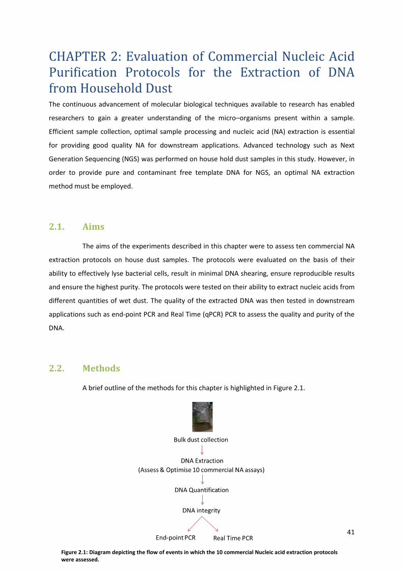
41

CHAPTER 2: Evaluation of Commercial Nucleic Acid Purification Protocols for the Extraction of DNA from Household Dust The continuous advancement of molecular biological techniques available to research has enabled

researchers to gain a greater understanding of the micro–organisms present within a sample.

Efficient sample collection, optimal sample processing and nucleic acid (NA) extraction is essential

for providing good quality NA for downstream applications. Advanced technology such as Next

Generation Sequencing (NGS) was performed on house hold dust samples in this study. However, in

order to provide pure and contaminant free template DNA for NGS, an optimal NA extraction

method must be employed.

2.1. Aims

The aims of the experiments described in this chapter were to assess ten commercial NA

extraction protocols on house dust samples. The protocols were evaluated on the basis of their

ability to effectively lyse bacterial cells, result in minimal DNA shearing, ensure reproducible results

and ensure the highest purity. The protocols were tested on their ability to extract nucleic acids from

different quantities of wet dust. The quality of the extracted DNA was then tested in downstream

applications such as end-point PCR and Real Time (qPCR) PCR to assess the quality and purity of the

DNA.

2.2. Methods

A brief outline of the methods for this chapter is highlighted in Figure 2.1.

Figure 2.1: Diagram depicting the flow of events in which the 10 commercial Nucleic acid extraction protocols were assessed.

42

2.2.1. Dust sample collection

House dust was collected with a vacuum cleaner. The dust was filtered through a coarse

sieve followed by a fine grid sieve to remove big particulate matter. Approximately 250 g of house

dust was collected. The dust was then stored in 20 g aliquots at 4°C.

2.2.2. DNA extraction from bulk house dust

A small amount of dry dust was placed in a 2 ml tube, and moistened with approximately

500 µl of 0.05% Tween 20. The wet dust was centrifuged at 14 000 rpm for one minute to remove

excess Tween 20. Specified amounts of wet dust were weighed out for each of the DNA extraction

protocols listed in Table 2.1.

Kit name Abbreviation Manufacturer

details

Catalogue

number

Recommended

starting

quantity

Recommended

Elution volume

(µl)

Z/R Fungal/Bacterial

DNA MicroPrep TM

ZMC Zymo research corp.,

Irvine, USA

D6007 10 -20 mg 10 – 20

Z/R Fungal/Bacterial

DNA MiniPrep TM

ZMN Zymo research corp.,

Irvine, USA

D6005 50 – 100 mg 25 - 100

Qiasymphony (DSP

Virus/bacteria midi kit)

QS Qiagen , Hilden,

Germany

937055 Not specified 60 ; 85 ; 110

FastDNATM Spin kit for

soil

FD MP Biomedicals,

Solon, USA

116560200 500 mg 50 - 100

NucleoSpin® Soil NS Macherey-Nagel,

Düren, Germany

740780/.50 250 – 500 mg 30 - 100

UltraClean® Microbial

DNA Isolation

UC MOBIO laboratories

Inc., Carlsbad, USA

12224-50 1.8 ml 50

UltraClean® Fecal DNA

isolation kit

UCF MOBIO laboratories

Inc., Carlsbad, USA

12811-50 250 mg 50

GenElute Plant

Genomic DNA Miniprep

Kit

GE Sigma–Aldrich

Chemie GmbH,

Steinheim, Germany

G2N10 100 mg 2 x 100

SoilMasterTMDNA

extraction kit

SM Epicentre®

Biotechnologies,

Wisconsin, USA

SM02050 100 mg 300

PowerSoil® DNA

Isolation kit

P MOBIO laboratories

Inc., Carlsbad, USA.

12888-50 250 mg 100

Table 2.1: Summary of the 10 commercial NA extraction protocols that were assessed in this study.

43

2.2.2.1. DNA extraction and optimisation

Initially, the lowest recommended starting wet weights (as per manufacturer’s

recommendation) were used for each of the protocols tested, with the exception of QS and UC, for

which the lowest starting wet weight used was amended to 50 mg (Claassen et al., 2013) and 100 mg

(1.8 ml weighed approximately 100 mg), respectively. Thereafter, each of the protocols were

optimised according to the manufacturer’s recommendations.

2.2.2.1.1. Sample lysis

Several lysis methods were used by the 10 NA extraction protocols including chemical,

mechanical as well as heat lysis (Table 2.2). Two of the NA extraction protocols namely, SM and GE

protocols incorporated a heat lysis step in addition to the mechanical lysis step (Table 2.2). Chemical

lysis for all the protocols were performed according to the manufacturer’s recommendation. In the

case of the NS protocol, an optimisation experiment, as recommended by the manufacturer, showed

that buffer SL1 allowed for optimal NA extraction from dust.

The mechanical lysis steps varied amongst the protocols with respect to instrumentation, time and

rigor (Table 2.2). The QiaSymphony (QS) protocol incorporated an off-board lysis step that includes

chemical and mechanical lysis steps (Claassen et al., 2013). Following the off-board lysis step, the

samples were loaded onto the QS SP instrument to continue with the automated NA extraction.

2.2.2.1.2. DNA elution volumes

The minimum elution volume as recommended by the manufacturer’s recommendations

were used for certain protocols (Table 2.2) where appropriate. The recommended minimum elution

volume was not applied in the following protocols: the P protocol made use of 50 µl elution volume

instead of 100 µl; and the SM protocol was amended from 300 µl to 50 µl. For the ZMC protocol, the

minimum elution volume of 10 µl was increased to 20 µl in order to obtain sufficient DNA for further

downstream applications and storage. The GE protocol recommended eluting in 2 x 50 µl elution

volumes, which were kept in two separate 1 ml Eppendorf tubes. According to each of these

protocols, the eluted DNA was ready-to-use for all standard downstream applications.

44

a. Bead beating using the tissue lyzer b. Horizontal bead beating using the vortex c. Mechanical lysis using the FastPrep® Instrument d. (65˚ pre-warmed elution solution) S – seconds Min – minutes

2.2.2.2. Modifications to DNA extraction methods

In addition to performing the NA extractions as per the manufacturer’s

recommendations, all of the NA extractions were also performed with two modifications. Firstly, in

addition to testing each of the protocols using the manufacturer’s recommended minimum starting

wet weight of dust, each NA extraction protocol was repeated using uniform starting weights of 100

mg, 50 mg and 20 mg of wet dust. The second modification entailed replacing the mechanical lysis

step of each protocol with a uniform mechanical lysis step using the TissueLyser LTTM (Qiagen,

FRITSCH GmbH, Idar-Oberstein, Germany) for two minutes at 50 Hertz (Hz).

ZMN ZMC NS FD SM GE UC UCF P QS

1.Wet weight dust (mg) 50 mg 10 mg 250 mg 500 mg 100 mg 100 mg 100 mg 250 mg 250 mg 50 mg 2

.Sam

ple

lysi

s

Chemical

Yes Yes Yes Yes Yes Yes Yes Yes Yes Yes

Mechanical 5 mina 50Hz

5 mina 50Hz

5 minb Speed 6.0

40 sc

Shake tube 37˚C

10 min

Vortex and

invert

10 minb 10 minb 10 minb 5mina 50Hz

Heat No No No No 65˚C 10 min

65˚C 10 min

No No No No

3.P

reci

pit

ate

lysa

te

Centrifuge 10 000 x g

1 min

10 000 x g

1 min

11 000 x g

2 min

14 000 x g

5 min

1000 x g

2 min

NA 10 000 x g

30 s

10 000 x g

30 s

10 000 x g

30 s

10 000 x g

1 min

Mechanical NA NA Vortex 5 s

Shake by hand 10

X

Invert tube by

hand

Inversion Vortex 5 s

Vortex 5 s

Vortex 5 s

NA

Incubation 4˚C 5 min

NA On ice 8 min

On ice 5 min

4˚C 5 min

4˚C 5 min

4˚C 5 min

Centrifuge 11 000 x g

1 min

13 500 rpm

8 min

12 000 x g

5 min

10 000 x g

1 min

10 000 x g

1 min

10 000 x g

1 min

4.Filter lysate Yes Yes Yes Yes Yes Yes Yes Yes Yes No

Bind Yes Yes Yes Yes Yes Yes Yes Yes Yes Magnetic particles

5.Wash 2 steps 2 steps 4 steps 1 step 2 steps 2 steps 1 step 1 step 1 step 1 step

6.Dry matrix NA NA NA 14 000 x g

2 min Air dry 5

min

NA NA 10 000 x g

1 min

10 000 x g

1 min

10 000 x g

1 min

No

7.E

luti

on

ste

p Incubation

with elution buffer

No 2 -3 min 1 min 5 min 55˚C

No No No No No No

Volume 25 µl 20 µl 30 µl 50 µl 50 µl 2 x 50µld 50 µl 50 µl 50 µl 60 µl

Table 2.2: Manufacturer’s recommendations for all NA extraction protocols used in this study.

45

All DNA extractions were performed in duplicate and the purified DNA was stored at 4°C until further

use.

2.2.3. Determination of DNA quality and integrity

The quality, quantity as well as integrity of the genomic DNA obtained from each of the

protocols were determined. DNA concentration and purity were determined on the Biodrop

spectrophotometer (Biodrop UK Ltd, Cambridge, UK) (Refer to Appendix B for protocol of steps

involved). The instrument was initially blanked with the relevant elution suspension. Thereafter, 1 µl

of genomic DNA was loaded onto the instrument and the DNA concentration was determined. Both

the DNA concentration (calculated using the 260 nm reading) and DNA purity (i.e., 260/280 nm ratio)

were assessed. A 260/280 nm ratio of ~1.8 is indicative of pure DNA, whereas a 260/280 ratio < 1.8

indicates contamination with humic acids (major organic constituent of soil), proteins (Steffan et al.,

1988) and phenols. A ratio of ~2 is indicative of RNA contamination (Nanadrop 2007).

The integrity of the DNA extracted with the various commercial protocols was visualised on 1%

horizontal agarose gels (w/v) (Lonza, USA), containing 0.5 µg/ml Ethidium Bromide (EtBr) and in 1X

TAE buffer (Appendix A, section I & II) (Refer to Appendix D for preparation of agarose gels). The

DNA samples were combined with a 5X loading buffer (Bioline, UK) before being loaded onto the gel.

Molecular weight marker, Hyperladder ITM (Bioline, UK) (Appendix E) was included on all agarose

gels.

Agarose gels were electrophoresed at 60 Volts (V) for 60 minutes. DNA was visualised on a UV

Transilluminator (UVITEC UV light box at 302 nm wavelength).

2.2.4. 16S rRNA gene end–point PCR

An end-point PCR assay targeting the 16S rRNA gene, made use of the following

degenerate primer pair: 1391R: 5’GACGGGCGGTGWGTRCA 3’ ; and 27F:

5’AGRGTTYGATYMTGGCTCAG3’ (Klindworth et al., 2013).

46

2.2.4.1. PCR positive control

A fresh stock of NCTC 8325 Staphylococcus aureus was cultured on a 2% blood agar plate.

A few colonies were removed from the 2% blood agar plate for DNA extraction using the ZMN

protocol. The DNA was quantified with the Qubit® dsDNA HS (High Sensitivity) Assay Kit

(InvitrogenTM, Carlsbad, CA, 92008, USA). The following DNA concentrations were included in an

optimisation PCR run to determine an optimal positive control concentration for further PCR assays:

3.4 ng/µl, 1 ng/µl, 0.5 ng/µl and 0.1 ng/µl.

2.2.4.2. 16S rRNA PCR optimisations

The following PCR optimisations were performed: varying the annealing temperatures

from 42˚C to 45˚C; and diluting template DNA for DNA extracted with the QS, NS and FD protocols,

in order to determine if PCR inhibitors were present in these samples. Template DNA dilutions

included 1:2, 1:5 and 1:10. Extra template DNA (extracted with the QS protocol) was tested in order

to determine whether sufficient template DNA was included in the PCR reaction.

2.2.4.3. Optimised 16S rRNA PCR protocol

DNA was extracted from 50 mg wet weight of household bulk dust, using the five best

protocols namely, ZMN, ZMC, NS, QS and FD. The PCR reaction mixture contained 1.5 U Gotaq

Polymerase (Promega, USA, CA), 1 x reaction buffer, 1.5 mM MgCl2 (GoTaq Flexi Buffer; Promeg,

USA, CA), 0.25mM dNTP’s (Thermo Scientific, USA,MA), 0.5µM of each 27F

(5’AGRGTTYGATYMTGGCTCAG3’) and 1391R (5’GACGGGCGGTGWGTRCA 3’) degenerate primers

(Klindworth et al., 2013) (Refer to Appendix C, section I for calculations of primer concentrations)

and 1 µl template DNA. PCR reactions were performed in 50 µl. DNA obtained from each NA

extraction protocol was tested in duplicate. PCR cycling conditions included an initial denaturation

step for 5 minutes at 95°C, followed by 30 cycles of 1 minute at 95°C, 30 sec at 43°C and 1 minute at

72°C. This was followed by 5 minutes at 72°C for final extension. The PCR reactions were performed

on the Applied Biosystems 2720 Thermocycler (Applied Biosystems, California, USA). The resultant

amplicons were electrophoresed on a 1% agarose gel (w/v) containing 0.5 µg/ml EtBr (Appendix D).

The approximate size of the amplicon is expected to be 1.36 kilobases (kb). A no-template control

(NTC) was included. The PCR positive control (PC) included genomic DNA isolated from

Staphylococcus aureus culture (DNA concentration of 0.5 ng/µl).

47

2.2.5. 16S rRNA gene qPCR

2.2.5.1. 16S rRNA qPCR optimisations

The following qPCR optimisations were performed: comparison of two master mixes,

namely iTaqTM Universal SYBR® Green Supermix (Bio-Rad Laboratories, Hercules, CA 94547, USA) and

Platinum® SYBR® Green qPCR SuperMix-UDG (InvitrogenTM, Carlsbad, CA, 92008, USA); comparison of

two PCR grade water stocks supplied from Life Technologies (CA, USA) and Roche (BASEL,

Switzerland); and finally, decreasing the number of cycles, from 40 cycles to 30 cycles. PC (0.5 ng S.

aureus genomic DNA) and NTC were included in the optimisation experiments.

2.2.5.2. Optimised 16S rRNA qPCR protocol

The five samples used in end-point PCR were used for qPCR. The qPCR reaction mixture

contained 1 x Platinum® SYBR® Green qPCR SuperMix-UDG (InvitrogenTM, Carlsbad, CA, 92008, USA),

0.4 µM of U16SRT-F 5‘ ACTCCTACGGGAGGCAGCAGT 3’ and U16SRT- R 5‘ TATTACCGCGGCTGCTGGC

3’ (Clifford et al., 2012) (Refer to appendix C, section II for calculations), and 1 µl of template DNA.

The qPCR reactions were performed in 20 µl volumes. DNA obtained from each NA extraction

protocol was tested in duplicate. The qPCR cycling conditions included: 50˚C for 2 minutes, 95 ˚C for

5 minutes and 30 cycles of 95 ˚C for 15 seconds, and 60 ˚C for 30 seconds, followed by the melt

curve analysis (as per the instruments default settings): 95 ˚C for 10 minutes, 65 ˚C for 5 seconds

using the CFX96™ Real-Time System (Bio-Rad Laboratories Inc., Hercules, CA, United States of

America). Every run included a NTC and a PC as described above.

2.2.6. Statistical analysis

Excel was used to graphically represent the number of replicates obtained for each

sample (one DNA extraction = one replicate). Through descriptive analysis, the range as well as the

mean of the duplicates within the replicate readings from the one sample (bulk house dust sample)

could be obtained. Box plots were obtained with the use of STATA version 13.1 (StataCorp LP, 4905

Lakeway Drive, College station, TX 77845, USA). Unconventionally, the box plot represents the

replicate DNA extractions from a single sample. Given the small sample size, non-parametric

methods of analysis were employed. The Wilcoxon signed-rank test was used to compare the

median concentration and purity to determine the best protocol. The comparison was made

between protocols performed according to the manufacturer’s recommendations, and protocols

performed with the modification (uniform mechanical lysis step). In addition, differences in the

48

median concentrations/purity of the five different protocols (averaged between replicate readings)

were assessed using the Kruskal-Wallis test. A p-value less than or equal to 0.05 was considered

statistically significant.

2.3. Results

2.3.1. Nucleic acid quality and integrity

2.3.1.1. Manufacturer’s recommendations

The lowest recommended starting weight of the ten protocols tested in this experimental

chapter ranged from 10 mg (ZMC) to 500 mg (FD) (Table 2.1). Amongst the commercial protocols

tested in this study, one recommended 50 mg, three recommended 100 mg and three

recommended 250 mg as the minimum amount of starting material (Table 2.1). The median DNA

concentration obtained using these lowest recommended starting weights were 7.96 ng/µl, with a

range from 1.29 ng/µl (GE) to 141.30 ng/µl (FD) (Figure 2.2A). The median DNA purity for this data

set was 1.62 (260/280) with a range from 1.00 (260/280) (UCF; GE) to 1.81 (260/280) (P) (Figure

2.2B).

Whilst the Powersoil DNA isolation protocol (P) yielded the purest DNA preparations at 250 mg

starting wet weight (Figure 2.2), the UltraClean fecal DNA isolation protocol (UCF) performed the

Figure 2.2: A) Bar graph representing the DNA concentrations of the 10 protocols performed according to the manufacturer’s specifications, at each of their lowest recommended starting wet weights. B) Bar graph representing the corresponding DNA purity of the 10 protocols performed according to the manufacturer’s specifications, at each of their lowest recommended starting wet weights. NAE 1: Nucleic acid extraction 1, NAE 2: Nucleic acid extraction 2.

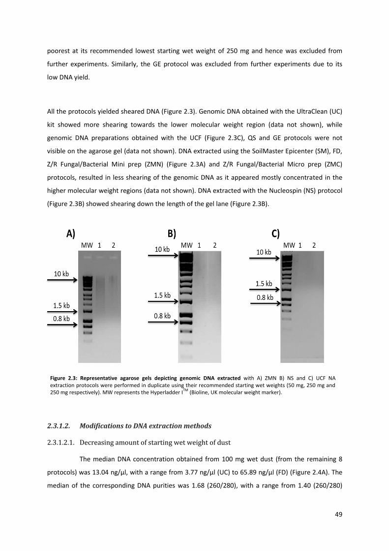
49

poorest at its recommended lowest starting wet weight of 250 mg and hence was excluded from

further experiments. Similarly, the GE protocol was excluded from further experiments due to its

low DNA yield.

All the protocols yielded sheared DNA (Figure 2.3). Genomic DNA obtained with the UltraClean (UC)

kit showed more shearing towards the lower molecular weight region (data not shown), while

genomic DNA preparations obtained with the UCF (Figure 2.3C), QS and GE protocols were not

visible on the agarose gel (data not shown). DNA extracted using the SoilMaster Epicenter (SM), FD,

Z/R Fungal/Bacterial Mini prep (ZMN) (Figure 2.3A) and Z/R Fungal/Bacterial Micro prep (ZMC)

protocols, resulted in less shearing of the genomic DNA as it appeared mostly concentrated in the

higher molecular weight regions (data not shown). DNA extracted with the Nucleospin (NS) protocol

(Figure 2.3B) showed shearing down the length of the gel lane (Figure 2.3B).

2.3.1.2. Modifications to DNA extraction methods

2.3.1.2.1. Decreasing amount of starting wet weight of dust

The median DNA concentration obtained from 100 mg wet dust (from the remaining 8

protocols) was 13.04 ng/µl, with a range from 3.77 ng/µl (UC) to 65.89 ng/µl (FD) (Figure 2.4A). The

median of the corresponding DNA purities was 1.68 (260/280), with a range from 1.40 (260/280)

Figure 2.3: Representative agarose gels depicting genomic DNA extracted with A) ZMN B) NS and C) UCF NA extraction protocols were performed in duplicate using their recommended starting wet weights (50 mg, 250 mg and 250 mg respectively). MW represents the Hyperladder I

TM (Bioline, UK molecular weight marker).

50

(SM) to 1.84 (P) (Figure 2.4D). Based on the purities and concentrations obtained, FD, ZMC, ZMN and

QS were the better performing protocols, whilst UC and SM were the worst (Figure 2.4A and 2.4D).

The median DNA concentration obtained from 50 mg wet dust was 11.00 ng/µl, with a range from

0 ng/µl (P) to 37.19 ng/µl (FD) (Figure 2.4B). The median of the corresponding DNA purities was 1.57

with a range from 0.00 (26/280) (P) to 2.44 (260/280) (NS) (Figure 2.4E). Based on the DNA

concentrations and corresponding DNA purities obtained from 50 mg starting wet weight of dust,

the FD protocol yielded the best quality DNA, whilst the P protocol was unable to yield detectable

levels of DNA, and hence was excluded from further experiments.

And lastly, the median DNA concentration for 20 mg wet dust was 8.44 ng/µl, with a range from

0 ng/µl (SM) to 34.15 ng/µl (FD) (Figure 2.4C). The median of the corresponding DNA purities is 1.61

(260/280) with a range from 0 (260/280) (SM) to 1.97 (260/280) (FD) (Figure 2.4F). The FD protocol

was able to yield the best quality DNA from 20 mg wet dust, followed by the ZMN and ZMC

protocols (Figure 2.4C & F). The SM protocol was the worst performing protocol at 20 mg wet dust

(Figure 2.6 C & F), which did not yield detectable levels of DNA.

51

Figure 2.4: Bar graphs A, B and C represent the DNA concentrations of the protocols performed according to the manufacturer’s recommendations at 100 mg, 50 mg and 20 mg, respectively. Bar graphs D, E and F represent the corresponding DNA purity of the protocols performed according to the manufacturer’s recommendations for 100 mg, 50 mg and 20 mg, respectively. NAE 1: Nucleic acid extraction 1, NAE 2: Nucleic acid extraction 2. The results obtained in figure 2.2, for ZMN and QS were repeated here in B, and E; and for: UC and SM were repeated in A and E.

52

2.3.1.2.2. Inclusion of a Uniform Mechanical Lysis step

Replacement of the recommended mechanical lysis step in each of the protocols with a

uniform mechanical lysis step did not reduce the amount of DNA shearing. A representative of such a

result can be seen in Figure 2.5. DNA extracted according to the manufacturer’s recommendations

(Figure 2.5, lanes 1 & 2) showed DNA shearing, while DNA extracted with the mechanical lysis

modification (Figure 2.5, lanes 3 & 4) showed no DNA on the agarose gel.

When the uniform mechanical lysis modifications were used with the recommended starting wet

weights per protocol, UC, P and UCF did not yield detectable levels of DNA (Figure 2.6C). Similarly,

when this modification was performed at 100 mg of starting wet weight, the UC and P protocols did

not yield detectable levels of DNA (data not shown). When performing P and UCF (according to both

the modification, as well as according to the manufacturer’s recommendations), they both did not

yield detectable levels for the 50 mg starting wet weight (data not shown). Protocols SM, GE, P and

UCF also did not yield detectable levels when performed on 20 mg starting wet weight (data not

shown).

Figure 2.5: Representative agarose gel image of NA extracted using the P protocol at a recommended starting weight of 250 mg. Lanes 1 and 2 represent genomic DNA extracted according to the manufacturer’s recommendations. Lanes 3 and 4 represent genomic DNA extracted with the mechanical lysis modification. Lane MW is Hyperladder I

TM (Bioline,

UK) molecular weight marker.

53

On average, 7/10 (70%) of the protocols performed better as per the manufacturer’s

recommendations at the recommended starting wet weights, when compared to the modified

protocols (i.e., inclusion of the mechanical lysis step) (Figure 2.6). The NS protocol performed better

when performed according to the manufacturer’s instructions (Figure 2.6). The UC, P and UCF

protocols were unable to yield detectable levels of DNA when performed according to the modified

protocol (Figure 2.6C & D). However, the SM, ZMC and GE protocols performed better according to

the modified protocol (Figure 2.6 C). When the modification was included, six of the ten protocols

yielded better DNA purities (Figure 2.6D). However, there is no statistical significance between the

manufacturer’s protocol and the modified protocol in terms of DNA concentration and purity (Table

2.3).

Figure 2.6: Bar graphs representing the DNA concentrations (A) and their corresponding purities (B) of the 10 protocols performed according to the manufacturer’s recommendations at their lowest recommended starting wet weights. Bar graphs representing the DNA concentrations (C) and their corresponding DNA purities (D) of the 10 protocols performed according to the uniform mechanical lysis step at their respective recommended starting wet weight. NAE 1: Nucleic acid extraction 1, NAE 2: Nucleic acid extraction 2.

54

Concentration

Purity Protocol Weight p50 (1) p50 (2) **P-value Protocol Weight p50 (1) p50 (2) **P-value

FD 20 18.59 13.12 0.14 FD 20 1.87 2.06 0.14

50 33.54 25.07 0.14

50 1.70 1.73 1.00

100 57.44 45.78 0.07

100 1.55 1.56 0.46

ZMC 20 14.22 10.59 0.27

ZMC 20 1.59 1.59 0.47

50 12.28 8.35 0.07

50 1.54 1.53 0.72

100 19.01 10.93 0.07

100 1.59 1.41 0.14

NS 20 10.25 8.07 0.27

NS 20 1.71 1.69 0.47

50 8.40 11.74 0.07

50 2.06 1.90 0.47

100 12.37 13.82 0.47

100 1.74 1.69 1.00

QS 20 3.63 2.08 0.27

QS 20 1.55 1.29 0.14

50 8.79 6.63 0.07

50 1.56 1.39 0.47

100 16.91 16.43 0.72

100 1.42 1.44 0.72

ZMN 20 15.39 10.70 0.14

ZMN 20 1.62 1.54 0.47

50 13.58 11.53 0.27

50 1.65 1.70 0.72

100 15.25 10.79 0.14

100 1.51 1.54 0.47

2.3.1.3. Comparison of the 5 best protocols using 50 mg wet dust

The FD, ZMC, ZMN, NS and QS protocols consistently yielded acceptable levels of DNA

(with reasonable DNA purity) from 100 mg down to 20 mg wet dust. The results above were

validated by repeating the NA extractions, in duplicate on 50 mg wet dust (Figure 2.7). The FD

protocol yielded the highest median concentration, whereas the NS protocol yielded the lowest DNA

concentration. However, the NS protocol yielded the highest the DNA purity, thus indicating RNA

contamination. FD and ZMN yielded the most optimal DNA purity (Figure 2.7).

**P-value of less than or equal to 0.05 is considered statistically significant P50 represent the median concentration/purity

(1) Represents the samples that were extracted according to the manufacturer’s recommendations (2) Represent the samples that were extracted according to our modification, where we added a mechanical lysis step

for 2 minutes at 50Hz using the tissue lyser

Table 2.3: Comparison between the median DNA concentration and purity, by protocol and weight between the manufacturer’s recommendations and the modified protocol (using the Wilcoxon signed rank test).

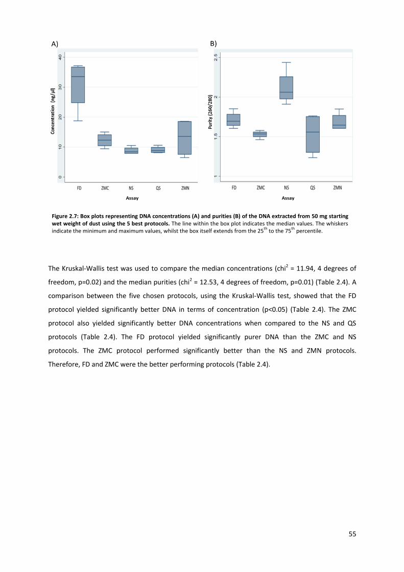
55

The Kruskal-Wallis test was used to compare the median concentrations (chi2 = 11.94, 4 degrees of

freedom, p=0.02) and the median purities (chi2 = 12.53, 4 degrees of freedom, p=0.01) (Table 2.4). A

comparison between the five chosen protocols, using the Kruskal-Wallis test, showed that the FD

protocol yielded significantly better DNA in terms of concentration (p<0.05) (Table 2.4). The ZMC

protocol also yielded significantly better DNA concentrations when compared to the NS and QS

protocols (Table 2.4). The FD protocol yielded significantly purer DNA than the ZMC and NS

protocols. The ZMC protocol performed significantly better than the NS and ZMN protocols.

Therefore, FD and ZMC were the better performing protocols (Table 2.4).

Figure 2.7: Box plots representing DNA concentrations (A) and purities (B) of the DNA extracted from 50 mg starting wet weight of dust using the 5 best protocols. The line within the box plot indicates the median values. The whiskers indicate the minimum and maximum values, whilst the box itself extends from the 25

th to the 75

th percentile.

56

Concentration

Protocol FD ZMC NS QS

z p z p z p z p

ZMC 2.31 0.02

NS 2.31 0.02 2.02 0.04

QS 2.31 0.02 2.02 0.04 -0.87 0.39

ZMN 2.31 0.02 0.00 1.00 -0.58 0.56 -0.58 0.56

Purity

Protocol FD ZMC NS QS

z p z p z p z p

ZMC 2.31 0.02

NS -2.31 0.02 -2.031 0.02

QS 0.58 0.56 0.00 1.00 2.31 0.02

ZMN 0.29 0.77 -2.32 0.02 2.32 0.02 -0.58 0.56

2.3.2. 16S rRNA gene end-point PCR

2.3.2.1. Positive control

DNA extracted from a fresh preparation of NTCC Staphylococcus aureus was quantified on

the Qubit® dsDNA HS (High Sensitivity) Assay Kit (InvitrogenTM, Carlsbad, CA, 92008, USA) and shown

to have a concentration of 3.4 ng/µl. The 16S rRNA end-point PCR performed on decreasing amounts

of S. aureus DNA indicated that 0.1 ng was the lowest concentration that could yield a detectable

PCR product of expected size, 1.36 kb (Figure 2.8). A concentration of 0.5 ng S. aureus DNA was

included as the positive control in all further 16S rRNA PCR experiments.

- P value of less than or equal to 0.05 is considered statistically significant. - A Z-score is a statistical measurement of a scores relationship to the mean. If the Z score is a 0, it means that the

score is the same as the mean, should it be a positive or negative, it means that it is either below or above the mean - P values indicated in bold are considered statistically significant

Table 2.4: Comparison between the 5 best protocols, in terms of purity and concentration at 50 mg starting wet weight (using the Kruskal-Wallis test).

57

2.3.2.2. 16S rRNA PCR protocol

DNA extracted with the ZMN and ZMC protocols yielded the best quality DNA for

endpoint PCR, as demonstrated in Figure 2.9. Even though the NS protocol produced similar DNA

concentrations to the ZMN protocol (Figure 2.4B), less PCR product was obtained using NS extracted

DNA. The FD protocol that yielded the highest DNA concentrations (Figure 2.4B) resulted in poor PCR

amplification. DNA extracted on the QS automated platform resulted in the poorest amplification

when compared to the other four protocols.

Figure 2.8: 16S rRNA PCR amplicons of the positive control, S. aureus, at decreasing template amounts. Amplicons were electrophoresed on a 1% agarose gel. Lane 1: 3.4 ng template DNA; lane 2: 1 ng; lane 3: 0.5 ng; lane 4: 0.1 ng. Lane MW: Hyperladder I

TM (Bioline, UK) molecular weight marker; lane NTC: No Template Control.

Figure 2.9: Representative agarose gel depicting 16S rRNA PCR amplicons using DNA extracted from 50 mg wet dust. Lanes 1-5: PCR amplicons from DNA extracted with the ZMN, ZMC, QS, NS and FD protocols, respectively. Lane MW: Hyperladder 1 molecular weight marker; Lane NTC and PC represent the no-template and positive control respectively.

58

2.3.2.3. 16S rRNA PCR optimisation tests

An annealing temperature of 43˚C resulted in an improved PCR amplification for the NS

and FD extracted DNA samples and hence was selected as the optimal annealing temperature to

continue with (Figure 2.9). Furthermore, adding 1 µl of genomic DNA to the PCR was the most

effective for PCR amplification for both NS and FD. However, none of the optimisation steps that

were carried out improved PCR amplification for QS extracted samples.

2.3.3. 16S rRNA gene SYBRgreen qPCR

2.3.3.1. 16S rRNA qPCR optimisation tests

Initial qPCR experiments, clearly showed amplification curves of the PC (Figure 2.10A).

Unfortunately, these experiments also showed amplification curves in the NTC starting after 30

cycles. The melt peak of the NTC falls within the melt peak of the PC (Figure 2.10B), suggesting

possible contamination.

Comparison of two different master mixes (iTaqTM Universal SYBR® Green Supermix (Bio-Rad

Laboratories, Hercules, CA 94547, USA) and Platinum® SYBR® Green qPCR SuperMix-UDG

(InvitrogenTM, Carlsbad, CA, 92008, USA), indicated that the Platinum® SYBR® Green qPCR SuperMix-

UDG (InvitrogenTM, Carlsbad, CA, 92008, USA) allowed slightly better amplification, as indicated by

the Cq values (PC has lower Cq and NTC has higher Cq values) (Figure 2.11). qPCR amplification of the

Figure 2.10: qPCR results of 1 PC, and 3 NTC’s. A) log scale of the amplification curves, B) melt peaks for the PC as well as the 3 NTC.

59

positive control was improved when an initial step of 2 minutes at 50˚C (for UDG incubation) was

included in the cycling conditions (data not shown). Changing the water supply for the qPCR assay

also improved amplification of the positive control (data not shown). The improvements were

indicated by a shift in the amplification curves, where the Cq value of the positive control decreased

and the Cq value of the NTC increased (data not shown).

2.3.3.2. 16S rRNA qPCR optimised protocol

The optimised qPCR protocol included Platinum® SYBR® Green qPCR SuperMix-UDG, PCR

grade water from Roche and cycling conditions for 30 cycles. DNA extracted with the five best

protocols was subjected to the optimised qPCR protocol.

A similar pattern of results was obtained to that seen in the end-point PCR assay. DNA extracted with

the ZMN, NS, ZMC, FD and QS protocols yielded amplification curves with mean Cq values of 15.48,

16.28, 16.60, 17.30 and 18,05 respectively (Figure 2.12A). The corresponding melt curves are

represented in Figure 2.12B, whereby all the melt temperatures (representing the PC amplicon and

amplicons generated from DNA extracted with all five protocols) fall within a range between 83.5 to

85˚C.

Figure 2.11: qPCR results comparing the 2 SYBR Green master mixes, Platinum® SYBR® Green qPCR SuperMix-UDG and iTaq

TM Universal SYBR® Green Supermix. A) log scale of the amplification curves, B) melt peaks for both master

mixes performed in triplicate. NTC refers to the no-template control and PC refers to positive control.

60

2.4. Discussion

When performing whole community studies, an optimal DNA extraction is key (Kennedy

et al., 2014). The DNA extraction process from dust and further downstream analysis is not

straightforward. Dust samples are known to include both Gram-positive as well as Gram-negative

bacteria. A proportion of the bacteria found in dust samples may contain hard-to-lyse cell walls. In

addition, dust samples may contain PCR inhibitors amongst other complex compounds. An efficient

DNA extraction protocol for environmental samples is important as studies have shown that variation

in the DNA yields that are used for library preparation may in fact impact on the variability of the

sequencing results (Gutiérrez-lucas et al., 2014; Kennedy et al., 2014).

Due to its ease of collection, dust samples are most commonly used in epidemiological studies of the

environment (Kärkkäinen et al., 2010). An array of methods have been implemented to collect dust,

including the use of an Electrostatic Dust fall Collector (EDC) (Noss et al., 2008), and the use of

vacuum cleaner bags (Täubel et al., 2009). The Drakenstein study makes use of EDC’s to collect dust

samples from indoor environments (shown in later chapters). However, preliminary experiments

indicated that minute amounts of dust were removed from the EDC’s, approximately 10 mg of wet

weight (Chapter 3). Therefore, for the purpose of assessing and comparing the ten commercial NA

extraction protocols, bulk dust collected with a vacuum cleaner was used. This allowed the same dust

sample to be used for all optimisations and evaluations. However, to simulate future experiments

that will make use of dust removed from EDC’s, 0.05% Tween 20 was added to the dry vacuum bulk

Figure 2.12: Final qPCR results of the 5 best protocols A) amplification curves and B) melt peaks of the 5 best protocols, assessed at 30 cycles. NTC refers to the no-template control and PC refers to positive control.

61

dust, as Tween 20 is used to remove dust off of electrostatic clothes (Noss et al., 2008; Normand et

al., 2009; Noss et al., 2010a; Noss et al., 2010b; Frankel et al., 2012; Madsen et al., 2012), thereby

producing wet dust.

Several different protocols have been used by others to extract DNA from dust samples. Protocols for

comparison were selected on the basis of prior use in similar studies (Roy et al., 2003; Täubel et al.,

2009; Maier et al., 2010; Yamamoto et al., 2011; Rittenour et al., 2012; Ettenauer et al., 2012; Guo

and Zhang 2013; Janke et al., 2013; Adams et al., 2014; Viegas et al., 2014;). These include:

GeneElute plant genomic DNA miniprep kit (Rintala et al., 2008; Kärkkäinen et al., 2010; Täubel et al.,

2009; Janke et al., 2013), Powersoil kit where the Earth Microbiome Project (EMP) made use of a

modified version of the protocol (Gilbert et al., 2014); Powersoil kit with the GeneElute kit (Janke et

al., 2013); and the FastDNA spin kit for soil (Maier et al., 2010; Ettenauer et al., 2012).

The aim of this chapter was to assess various NA extraction protocols for the purification of DNA

from small amounts of wet dust. In addition, the extracted DNA must be of good quality, so that it

could be used in downstream applications (such as end-point, real time PCR, as well as next

generation sequencing).

This study assessed ten commercial NA extraction protocols, which included the GE, FD, P, ZMC,

ZMN, NS, QS, UC, UCF and SM protocols. Each of the protocols were initially performed as per the

manufacturer’s recommendations. In addition, each protocol was repeated with a modification,

whereby the recommended mechanical lysis step was replaced with a uniform mechanical lysis step

(50 Hz for 2 minutes on the Tissue-lyser) so as to create uniformity across all the protocols. Inclusion

of this step did not improve DNA yield, or purity (Figure 2.6), nor did it reduce the amount of DNA

shearing (Figure 2.5). Hence, only the results obtained from protocols performed with the

manufacturer’s recommended mechanical lysis steps are discussed further.

All the protocols were performed using the manufacturer’s recommended lowest starting weight of

wet dust as well as adjusting the starting wet weights to 100 mg, 50 mg and 20 mg. Reduction of the

starting material allowed the identification of NA extraction protocols that can efficiently extract

DNA from low quantities of dust. Prior optimisation experiments performed in our laboratory

62

indicated that settled dust samples weigh very little, as low as 10 mg. Therefore, a protocol that can

extract NA from low quantities of dust most efficiently would be ideal.

Amongst the 10 protocols evaluated in this study, five protocols were eliminated based on their

performance, namely, P, SM, GE, UC and UCF protocols. Despite yielding the most pure DNA

preparation from 250 mg (recommended lowest starting weight) wet dust (Figure 2.2B), the

PowerSoil protocol was unable to extract detectable levels of DNA from 50 mg of wet dust (and

lower quantities) (Figure 2.4B & E). In contrast, Janke et al., (2013) was able to extract fungal DNA

from 500 µl of fungal spore suspension, which is equivalent to more than 100 mg of wet dust, using

the GE and P protocols (with P being the preferred choice). The UCF protocol could not consistently

extract DNA from the recommended lowest starting weight (250 mg) (Figure 2.2), possibly due to the

difference in the nature of the starting material, viz., dust as opposed to faeces. In addition, the DNA

could not be visualized on an agarose gel, confirming the low levels of DNA extracted from 250 mg of

wet dust (Figure 2.3). Faecal samples might require a stringent mechanical lysis step, which could

have contributed to the negative results obtained for dust. However, implementation of a less

stringent mechanical lysis step, did not improve DNA yield for the UCF protocol (Figure 2.6C &D).

The GeneElute and FastDNA protocols are the most commonly used DNA extraction kits in literature

for the isolation of DNA from dust samples (Rintala et al., 2008; Täubel et al., 2009; Maier et al.,

2010; Ettenauer et al., 2012; Janke et al., 2013). However, in this study, the GE protocol yielded

impure DNA (260/280 ratio between 1 and 1.3) and could not extract detectable levels of DNA from

20 mg of wet dust (data not shown). Täubel et al., (2009) was able to extract detectable levels of

DNA from 25mg of dry dust, which may contain more dust particles than 20 mg of wet dust (where a

significant part of the weight is due to the moisture in the sample). Similar to the UCF protocol, DNA

extracted with the GE protocol could not be visualized on an agarose gel, confirming the

undetectable levels of DNA obtained with this protocol (data not shown).

Suarez Martinez et al., (2006) compared several NA extraction protocols for the isolation of NA from

dust samples. This study showed that the SoilMaster protocol (Epicentre) was most efficient at

extracting DNA from dust samples and that the DNA could be used for the detection of bacteria,

fungi and dust mites. Although the SM protocol yielded detectable levels of DNA with better purities

than that obtained with the GE protocol, the SM protocol was unable to yield detectable levels of

DNA of from 20 mg of wet dust (Figure 2.4C & F). The major difference between this study and the

63

Suarez Martinez et al., (2006) study is the amount of dust used for DNA extraction, 100 mg (Suarez

Martinez et al., (2006) study) versus 20 mg (this study). The fifth and final protocol which was

excluded from further testing, the UltraClean protocol, was able to extract detectable levels of DNA

from all the quantities of dust, however, it did so at the expense of the DNA purity (Figure 2.4). Also,

the integrity of the DNA was compromised, due to more DNA shearing observed in the lower

molecular weight region on the agarose gel (data not shown). The extensive DNA shearing could be

due to the mechanical lysis step, which may have been too harsh on the dust samples. Dust is a very

fine material in comparison to soil. Rittenour et al., (2012) showed that the DNA extracted from dust

with the UC protocol not only contained PCR inhibitors, but also that the UC protocol is biased

against certain fungi, such as Aspergillus.

The five remaining protocols namely, ZMN, ZMC, FD, NS and QS protocols were selected for further

evaluations, based on their performance. The FD, ZMN and ZMC protocols, were able to consistently

extract detectable levels of DNA (amongst the highest concentrations obtained in this study) from

the dust sample, with an improved DNA purity as the dust quantity decreased (Figure 2.4D-F).

Furthermore, these three protocols yielded DNA with the least amount of shearing, when compared

to the other protocols in this study, as most of the DNA was concentrated in the high molecular

weight region of the agarose gel (representative for ZMN in Figure 2. 3A). The NS protocol was able

to extract DNA from as little as 20 mg of wet dust (Figure 2.6), bearing in mind that the NS lowest

recommended starting weight is 250 mg (Table 2.1). However, the DNA extracted with the NS

protocol appeared uniformly sheared down the gel lane (Figure 2.3B). The fifth protocol included in

further evaluations, namely the QS protocol, was able to extract good quality DNA (in terms of DNA

concentration and purity) from all the dust quantities (Figure 2.4). Also, the QS protocol is the only

automated protocol included in this study.

Based on the box plots obtained (Figure 2.7) as well as the Kruskal-Wallis test (Table 2.4), FD

performed significantly better than ZMC and NS. However, the ZMC protocol performed significantly

better than NS. The limitation of this study was that the sample size was one (one bulk house dust

sample that was used to test the different protocols). Taking that into account, when the Kruskal-

wallis test was done, where a p-value of less than or equal to 0.05 is considered significant, this in

fact should change to 0.005. If this amended significance value were to be included, then none of the

protocols would be seen as significantly different from one another. Hence, for the purpose of this

study, a p-value of 0.05 was defined as statistically significant.

64

The five best protocols were assessed further in order to determine the quality of the DNA

preparations. The DNA from the five protocols was subjected to end-point PCR and qPCR. DNA,

extracted from 50 mg wet dust with the five chosen protocols, were subjected to 16S rRNA PCR using

previously described degenerate primers (Klindworth et al., 2013) for endpoint PCR as well as for

SYBR Green qPCR assay (Clifford et al., 2012). All bacteria harbour at least one copy of the 16S rRNA

gene. The selected primer sets have been shown to target the majority of bacteria in the SILVA

database. The end-point PCR assay targeted a 1.3 kb region of the 16S rRNA gene (Klindworth et al.,

2013) (confirming the good quality of the DNA for most protocols even though the DNA was

sheared).

Endpoint PCR results showed that DNA prepared with the ZMN and ZMC protocols was most suitable

as these DNA preparations allowed for optimal PCR amplification (Figure 2.9). Although the FD

protocol yielded the highest DNA concentration and purity, PCR amplification using this DNA

preparation was poor (Figure 2.9), suggesting the presence of PCR inhibitors or fragmentation.

Dilution of the DNA did not improve the PCR amplification (data not shown). Both the NS and ZMN

DNA samples were comparable in DNA concentration (Figure 2.4B &E), yet the ZMN-extracted DNA

was amplified more efficiently (Figure 2.9). Similarly, the NS and QS extracted DNA had similar DNA

concentrations, yet the QS -extracted DNA performed the worst in end-point PCR (Figure 2.9),

suggesting possible PCR inhibitors present in the QS preparation. Diluting the QS prepared DNA did

not improve the PCR amplification (data not shown).

In an attempt to improve PCR amplification using DNA extracted with the NS, FD and QS protocols,

PCR optimisation experiments were performed. Humic acids act as potent PCR inhibitors, resulting in

either complete failure of enzymatic downstream applications (such as PCR) or lowering the

sensitivity of the PCR assay. However, humic acid contamination can be reduced by diluting the

isolated DNA prior to PCR analysis. Dilution of the DNA extracted with the NS and QS protocols did

not improve PCR amplification, suggesting that inhibition was not the sole reason for poor

amplification.

Real time PCR, also known as qPCR is a more sensitive technique than endpoint PCR and it is

commonly used for microbiological analysis (as indicated in the literature review). Clifford et al.,

(2012) designed a set of primers based on the consensus sequence of an alignment of 962 279

bacterial 16S rRNA gene sequences. These primers target a 180 bp fragment and are reported to

65

anneal to 93.6% of the bacterial 16S rRNA genes in the Ribosomal Database Project release 10 (Cole

et al., 2009).

The qPCR results were concordant with the results of the end-point PCR for the ZMC and ZMN

protocols where very good amplification curves (mean Cq values of 15.48 and 16.60, respectively)

were obtained. DNA prepared with the NS protocol also amplified well (Cq value of 16.28) (Figure 2.

12), which was in contrast to the findings of end-point PCR, where only a very faint band was visible

(Figure 2.9). A possible reason for this difference could be due to a smaller amplicon (100 bp)

generated in the qPCR assay, compared to a larger amplicon generated during end-point PCR (1.36

kb). Similarly, amplification of DNA extracted with the QS and FD protocols yielded better results

than the end-point PCR (Figure 2.12). This could be because qPCR is more sensitive than end-point

PCR or because the smaller amplicon size permitted amplification of more highly fragmented DNA.

Our results with regards to the FD protocol are similar to those of Maier et al., (2010), who showed

that DNA extracted from dust (21 – 35 mg) using the FD protocol could be used in downstream

applications such as 16S rRNA PCR DGGE. Upon diluting the template DNA obtained with the FD

protocol, an improvement in the mean Cq value was obtained (data not shown), indicating the

presence of inhibitors, and possibly why poor amplification was observed in the end-point PCR

(Figure 2.9).

When optimising for the qPCR, two different master mixes were compared. The master mix

containing UDG (Platinum® SYBR® Green qPCR SuperMix-UDG (InvitrogenTM, Carlsbad, CA, 92008,

USA)) was considered superior (Figure 2.12). UDG and UNG catalyzes the hydrolysis of the N-

Glycosylic bond between sugar and uracil within DNA, thereby preventing carry-over of amplicon

DNA in PCR reactions. Inclusion of the UDG containing master mix increased the Cq value for the

NTC, suggesting reduced contamination (Figure 2.11). According to Shen et al., (2006) commercially

available purified water contains low levels of L. pneumophila DNA that may have escaped the

purification process. For this reason, Nuclease free water from Life Technologies (CA, USA) and from

Roche (BASEL, Switzerland) were compared in the qPCR assay. Results indicated that nuclease free

water supplied by Roche delayed amplification in the NTC (Figure 2.11). Although the inclusion of

UDG containing master mix and Roche nuclease free water delayed the amplification in the NTC,

amplification was still visible after 30 cycles of PCR. Amplification of the NTC could be due to a

number of reasons, including contamination of primer mixes, PCR water or master mix, and is not

uncommon for highly sensitive 16S rRNA PCR.

66

2.5. Conclusion

Ten commercial NA extraction protocols were evaluated using decreasing quantities of

wet bulk house dust. Five of the protocols (ZMC, ZMN, NS, QS and FD) consistently yielded DNA from

20 mg wet dust, which is lower than the recommended minimum starting weight for most of these

protocols. Based on the DNA concentration and purity, good quality DNA was obtained from these

five protocols. In addition, the ZMC protocol was able to consistently extract good quality DNA from

as low as 10 mg (i.e., the lowest recommended starting wet weight of this protocol) of wet dust. End-

point PCR indicated possible PCR inhibitors present in DNA extracted with the QS, NS and FD

protocols, while DNA extracted with the ZMC and ZMN protocols allowed optimal end-point PCR

amplification. However, DNA from all five protocols performed equally well in the qPCR assay.

67

CHAPTER 3

Optimization of Dust Sample Collection and Pre-analytical Processing

68

CHAPTER 3: Optimization of Dust Sample Collection and Pre-analytical Processing Studies involving sample collection, whether it is for clinical specimens or environmental samples,

require the appropriate aseptic procedures to be in place. This is to ensure that samples are collected

free from contaminants. Hence it’s important to ensure that the collection apparatus are sterile or

clean of any contaminating micro-organisms before use. The experiments conducted in this chapter

made use of Ultraviolet Germicidal Irradiation (UVGI) to sterilise electrostatic cloths, prior to

placement for collection of household dust. Following dust collection, removal of dust from these

electrostatic cloths was optimised for further downstream processing (i.e., DNA extraction, end-point

PCR, Next Generation Sequencing).

3.1. Aims

The aims of the experiments described in this chapter were to assess and optimise sample collection

and processing. The following processes were assessed:

1) Verifying that the sterilisation procedure of the EDC is effective

2) Optimising dust removal from the EDC as well as determining whether sufficient dust

was obtained for DNA extraction

3) Optimising the DNA extraction procedure using the Z/R Fungal/Bacterial DNA

MicroPrepTM protocol (ZMC) to ensure that sufficient DNA was obtained for downstream

applications such as NGS.

3.2. Methods

3.2.1. Preparation and sterilization of Electrostatic Dust Collectors (EDC’s)

Plastic folders (prime LINE, Poly Propylene Quotation Folder W432, Waltons, SA) were

sterilised with 70% EtOH within a class II biosafety cabinet (UV light off). Both the outside and inside

of the folders were wiped with 70% EtOH. Each folder was opened and an electrostatic cloth

(Changzhou Daya Imp & Exp Corp Ltd) was attached to both sides of the folder with a staple at each

corner. This defines an electrostatic dust collector (EDC) (Figure 3.1).

69

Opened EDC’s together with the A4 envelopes (B4 Croxley, Envelopes, 250 mm x 353 mm, ENP99CC

White, Waltons, SA) (in which the sterile EDC was to be stored) were placed in the class II biosafety

cabinet with the UV light switched on for 30 minutes, in order to UV irradiate the EDC’s and

envelopes (Figure. 3.2). The UV lamp was switched off after 30 minutes, the folders were closed, a

label was placed on the outside of the folder as well as on the envelope. The sterilized EDC was

placed inside the A4 envelope and the closed envelope was removed from the class II biosafety

cabinet to be stored in a cool dry place or to be sent out to the sites for placement. The label placed

on the EDC and the envelope were identical and contained information pertaining to placement of

the EDC.

3.2.2. Assessment of the EDC sterilisation process

Sterilization efficiency was assessed by processing the EDCs in three different ways: 1) An

EDC was opened inside a UV cabinet, exposing the electrostatic cloths to UV radiation for 30

minutes. The irradiated EDC was placed into an A4 envelope (irradiated along with the EDC), the

envelope closed and removed from the UV cabinet. This sterilized EDC was processed immediately to

assess the sterilization process (UV treated EDC (New)) (as explained above, section 3.2.1). 2) An EDC

Figure 3.2: EDC UV sterilisation.

Figure 3.1: Representative image of an EDC.

70

was opened inside a UV cabinet, exposing the electrostatic cloths to UV radiation for 30 minutes. The

irradiated EDC was placed into an A4 envelope (irradiated along with the EDC); the envelope was

closed and removed from the UV cabinet. This sterilized EDC was stored for approximately 4 – 6

months, in a cool place before being processed to assess the sterilization process (UV treated EDC

(stored)). 3) Several electrostatic cloths were wrapped in aluminium foil and sterilised by autoclaving

(Autoclave Only). 4) As a control, an electrostatic cloth was included that was not sterilised

(Untreated EDC).

The sterility of the EDC treatments (above) was assessed as shown in Figure 3.3: 1) A sterile swab was

immersed in 0.05% Tween 20 (Promega Corporation, MA, USA), brushed across the surface of the

electrostatic cloth and then spread onto a blood agar plate (National Health Laboratory Services,

Greenpoint, CT). 2) A swatch was cut out of the same electrostatic cloth and placed in the middle of a

blood agar culture plate. 3) The remainder of the electrostatic cloth was immersed in 100 ml 0.05%

Tween 20 and placed on an orbital shaker for 30 minutes at 160 rpm (Revolutions Per Minute). An

aliquot of 100 µl of this wash suspension was spread onto a blood agar plate. Lastly 4) the remainder

of the EDC/Tween 20 wash suspension was poured into a sterile 50 ml blue capped tube and

centrifuged at 2500 g for 15 minutes. Most of the supernatant was aspirated and discarded. An

aliquot of 100 µl of the concentrated dust wash solution was spread onto a blood agar plate.

All blood agar plates (including a “control” culture plate, which was an unused sterile BA agar plate)

were incubated in a 5% Carbon Dioxide (CO2) incubator for 18 to 24 hours, after which it was

assessed for microbial growth. If no growth was present, they were left to incubate for another 24

hours.

71

3.2.3. Optimisation of dust removal from EDC’s

Sterile EDC’s were placed in the homes of five work colleagues for a duration of two

weeks to collect settled dust. These five EDC’s were used to optimise dust removal from the EDC’s.

Dust removal from the EDC’s was adapted from the protocol outlined by Noss et al., (2008), which

entails shaking the EDCs in a sterile glass beaker, containing 0.05% Tween 20 (Promega Corporation,

MA, USA), for 45 minutes at room temperature. The dust suspension was then centrifuged at 7 500

rpm for 15 min at 22°C (Biovac Neofuge 15R, Vacutec, SA) (Noss et al., 2008; Madsen et al., 2012).

The adapted protocol for dust removal (Figure 3.4) was as follows: 1) Within the biosafety cabinet, an

electrostatic cloth was removed from the plastic folder using sterile stapler removers, 2) the cloth

was placed in a 1 litre (L) sterile beaker, 3) 100 ml of 0.05% Tween 20 was added to the beaker (the

volume of the Tween 20 was increased because the cloth used in this study was bigger than the cloth

used by Noss et al., (2008)), 4) the beaker was closed with aluminium foil, removed from the

biosafety cabinet, and placed on the orbital shaker (OrbitTM 1900, Labnet International, Inc., NJ,USA)

for 45 minutes at 160 rpm, 5) transferring the closed beaker back into the biosafety cabinet, the foil

was removed, 6) the cloth was lifted out of the dust/Tween 20 suspension (held over the beaker

using sterile forceps) and rinsed using a sterile Pasteur pipette (the dust/Tween 20 suspension was

used to rinse any visible particles off of the cloth into the beaker), 7) The cloth was removed from the

Figure 3.3: Assessment of the EDC sterilisation process.

72

beaker and discarded, 8) approximately 45 ml of the dust/Tween 20 suspension was poured into a

sterile 50 ml tube (CellSTARR Tubes, Greiner bio-one, Sigma–Aldrich Chemie GmbH, Steinheim,

Germany) and centrifuged for 15 minutes at 4˚C at 7 500 rpm, 9) the supernatant was discarded, and

the remainder of the dust/ Tween 20 suspension was added to the “pellet” in the tube, 10) this was

once again centrifuged for 15 minutes, at 4˚C at 7 500 rpm, the supernatant discarded, leaving

behind approximately 2 ml of Tween 20 suspension above the pellet. 11) The dust/Tween 20 mixture

was transferred to a pre-weighed 2 ml tube (Sarstedt AG & Co, Nümbrecht, Germany) and

centrifuged at 4 500 rpm for 5 minutes (Centrifuge 5417C, Merck Millipore, MA, USA), the

supernatant discarded and a final centrifugation step was employed to ensure efficient separation

between the dust and the Tween. The remainder of the supernatant was aspirated, leaving behind a

compact dust pellet. The 2 ml tube was weighed once more to calculate the mass of the dust pellet.

An amount of 10 mg wet weight was removed for DNA extraction, and the remainder of the dust (if

any) was stored at -80˚C in 25 % glycerol (Kimix chemical and Laboratory Supplies, CT,SA).

Figure 3.4: Flow diagram depicting the removal of dust from the electrostatic cloth.

73

3.2.4. DNA extraction

3.2.4.1. Optimization of DNA extraction using bulk dust

Optimisations of the ZMC protocol for DNA extraction from low quantities of dust were

conducted on bulk dust. The ZMC protocol was amended in various ways (Figure 3.5) in an attempt

to either increase DNA yield, or avoid loss of sample (because according to the manufacturer’s

protocol, only half of the sample is used for the DNA extraction). The following optimisations were

conducted, using 10 mg of starting wet weight. 1) As per the manufacturer’s recommendation: The

ZMC protocol was performed as outlined by the kit instructions, which entailed 400 µl of the

supernatant being loaded onto the spin column, and the remaining 400 µl of the supernatant being

discarded. 2) All sample: The entire 800 µl of supernatant was transferred to the spin column

(therefore not wasting any sample). 3) According to the manufacturer’s recommendation x 2: 400 µl

of the supernatant was added to the spin column as outlined in the kit instructions (3a), however,

instead of discarding the remainder of the supernatant, it was added to another spin column (3b).

The DNA extractions were carried out in parallel, with the end product being 2 x 20 µl of PCR ready

DNA (instead of 1 x 20 µl). And lastly, 4) According to the manufacturer’s recommendation x 2

concentrated: DNA extractions were carried out same as in step 3, however, the eluted DNA was

pooled together into the same collection tube (therefore, 1 x 40 µl of “concentrated” eluted DNA).

Each of these optimisation steps were carried out in duplicate. DNA concentrations were calculated

with the use of the Qubit® dsDNA HS (High Sensitivity) Assay (InvitrogenTM, Carlsbad, CA, 92008, USA).

74

Figure 3.5: Flow diagrams depicting the various optimisation steps that were carried out for the ZMC protocol. Method 1 depicts the recommended manufacturer’s method; methods 2-4 show the adaptations made to the manufacturer’s method (variations circled in red).

75

3.2.4.2. DNA extraction from dust removed from the EDC’s

DNA was extracted from the five EDCs described in section 3.2.3. The DNA was extracted

according to method 3 (above), and the Qubit® dsDNA HS (High Sensitivity) Assay (InvitrogenTM,

Carlsbad, CA, 92008, USA) was used to quantify the DNA.

3.2.5. 16S rRNA end-point PCR optimisation using DNA extracted from bulk dust

Optimisation of the 16S rRNA end-point PCR was performed on the DNA that was

extracted from 10 mg to 20 mg starting wet weight from the bulk dust samples. These samples were

prepared using the ZMC protocol, where the DNA extractions were performed in duplicate according

to their manufacturer’s recommendations using the ZMC protocol. The DNA concentrations were

obtained with the use of the Qubit® dsDNA HS (High Sensitivity) Assay (InvitrogenTM, Carlsbad, CA,

92008, USA) as previously mentioned.

Preparation of the PCR reaction as well as PCR cycling conditions was conducted as per chapter 2.

The resultant amplicons were electrophoresed on a 1% agarose gel (w/v) containing 0.5 µg/ml

(EtBr). The approximate size of the amplicon was expected to be 1.36 kilo bases (kb). A no-template

control (NTC) was included. The PCR Positive control (PC) included genomic DNA isolated from a

Staphyloccocus aureus culture (DNA concentration of 0.5 ng/µl) (used in chapter 2).

PCR optimisations were required in order to improve PCR amplification from DNA extracted (with

the ZMC protocol) from 10 to 20 mg starting wet weight. Hence, less template DNA was used, as

opposed to the amount used in Chapter 2 (DNA extracted from 50 mg wet dust). PCR optimisations

included template dilutions (1:2 and 1:10); increased template amounts (1 µl, 2 µl and 5 µl);

increased PCR cycles (from 30 to 35 cycles); and evaluating different PCR master mixes.

The three PCR master mixes that were assessed included: 1) GoTaq PCR reagents (1.5U GoTaq

Polymerase (Promega, USA, CA), 1x reaction buffer, 1.5mM MgCl2 (GoTaq Flexi Buffer; Promeg, USA,

CA),0.25 mM dNTP mix (KAPA Biosystems), 2) 1x Kapa Hotstart readymix (Kapa Biosystems, MA,

USA); and 3) 1x GoTaq® Green master mix (Promega, USA, CA). Each of the three PCR master mixes

also contained 1.25 µl of each 27F (5’AGRGTTYGATYMTGGCTCAG3’) and 1391R

(5’GACGGGCGGTGWGTRCA 3’) degenerate primers (Klindworth et al., 2013) (Refer to Appendix C,

76

section I for calculations of primer concentrations) and 1 µl template DNA (extracted DNA). The

reaction mixture contained a final volume of 25 µl per reaction. These master mixes were tested

using DNA extracted from both 10 and 20 mg of wet dust. The PCR cycling conditions were the same

as described in chapter 2 section 2.2.4.3.

The optimised PCR protocol (above) was performed using DNA extracted from EDC-collected dust. A

16S rRNA end-point PCR was performed using the Kapa master mix and 2 µl of template DNA.

3.3. Results

3.3.1. Assessment of the EDC sterilisation process

The untreated electrostatic cloths yielded bacterial growth on the Blood agar (BA) plate

(Table 3.1). Both the untreated cloth and UV treated EDC (new) showed fungal growth on the BA

plate. The UV treated EDC (stored) and autoclaved electrostatic cloths showed no microbial growth

on BA plates. No growth was observed on the “control” culture plate.

3.3.2. Dust removal and DNA quantification from EDC’s

Dust removal from the EDC’s was adapted from the protocol developed by Noss et al.,

(2008). The adaptations allowed for a dense dust pellet to be formed at the bottom of the cryogenic

tube, and hence, allowing a more accurate weight of the wet dust to be obtained. The average wet

Table 3.1: Bacterial and fungal growth from treated electrostatic cloths

a- Fungus present after 1 week - no growth - growth

77

weight of dust obtained from the five EDCs was 10 mg. The total amount of DNA extracted from 10

mg of wet dust ranged from 1.2 ng to 8.14 ng (Table 3.2), where the last column in table 3.2

represents total DNA yield from a single DNA extraction.

3.3.3. Optimisation of the ZMC DNA extraction protocol using bulk dust

The ZMC protocol was the chosen commercial protocol to proceed with for the extraction

of NA from dust, as it can purify DNA from wet dust with a starting wet weight of 10 mg (Chapter 2).

However, the protocol ultimately uses half of the starting weight of sample specified (Figure 3.5,

Method 1). Loading the entire 800 µl of sample/lysis buffer suspension (method 2, Figure 3.5) onto

the ZymoSpin IV column resulted in a very low DNA yield when compared to the first method (Table

3.3). However, when two ZymoSpin IV columns were used in order to process the entire sample

(Method 3, Figure 3.5), better DNA yields were obtained (Table 3.3), regardless of whether the DNA

was eluted in separate tubes (Method 3 in Table 3.3, and Method 3 in Figure 3.5) or eluted in a

single tube (Method 4 in Table 3.3, and Method 4 in Figure 3.5). The better option was method 3, as

it provided more DNA in total (Table 3.3).

Table 3.2: Starting wet weight of dust and total DNA obtained for the 5 EDC’s

Table 3.3: Comparison of the total DNA (ng) obtained from 10 mg wet dust (in duplicate) using the adapted ZMC DNA extraction methods.

78

3.3.4. 16S rRNA end-point PCR

3.3.4.1. 16S rRNA end-point PCR optimisations on DNA extracted from bulk dust

End-point PCR using the DNA extracted from 10 mg and 20 mg of bulk dust as template

failed to produce PCR amplicons (data not shown). Increasing the number of PCR cycles had no

effect. Similarly, no PCR amplicons were obtained when the template DNA was either diluted or

increased in amount (data not shown). The PCR positive and no-template controls worked under the

PCR conditions employed (Section 3.2.5).

Changing the PCR components had an effect on the PCR. Changing the dNTP stock (from Thermo

Scientific to KAPA Biosystems) resulted in faint PCR amplicons visible on the agarose gel (Figure

3.6B). Changing the entire master mix (from GoTaq to KAPA Hotstart readymix) resulted in very good

PCR amplification (Figure 3.6A).

Figure 3.6: Agarose gel depicting the 3 different master mixes assessed. Numbers 1 and 2 represents the 10 and 20 mg respectively for the GoTaq Matermix; 3 and 4 represents the 10 and 20 mg respectively for the Kapa Matermix and 5, 6 (10 mg),7 and 8 (20 mg) for the master mix with the KAPA dNTPs.

79

3.3.4.2. Optimised 16S rRNA end-point PCR using DNA extracted from EDC’s

End-point PCR set up with the Kapa Hotstart readymix resulted in PCR amplification from

all five EDC’s (Figure 3.7). The PCR included DNA extracted from 10 to 20 mg of dust that was

removed from EDCs. All five EDCs rendered sufficient dust as well as good quality DNA for PCR

amplification.

3.4. Discussion

The terms “house dust” and “settled dust” are used to describe particulate matter that

has been collected on flat surfaces. This dust that collects on these surfaces contains a variety of

constituents in different amounts, relative to the buildings location, surroundings, as well as the

activities of the inhabitants (Macher, 2001). Dust that is collected from settled surfaces is considered

to have once been airborne dust, and therefore is a more adequate representation of airborne

exposure in comparison to dust retrieved from floors and mattresses (Noss et al., 2008).

Furthermore, settled dust is so fine and light in weight, the time required to accumulate sufficient

dust to answer a research question can vary from weeks to months, depending on the question

asked and the amount of dust required for the study. There are a number of ways of collecting

settled dust, including vacuum cleaners and electrostatic cloths or electrostatic dust collectors (EDC).

In this study, settled dust was collected according to the method outlined by Noss et al., (2008), by

the use of an EDC.

Figure 3.7: Agarose gel depicting the PCR amplicons obtained using the KAPA master mix. Template DNA was extracted from 10 -20 mg wet dust removed from the 5 EDC’s.

80

Ultraviolet germicidal irradiation (UVGI) has been accepted as a sterilisation procedure since the

mid-20th century, and has been indicated as an effective sterilisation and disinfecting agent against

spore forms and vegetative forms of bacteria (Dietz et al., 1980; Blatchley & Peel 2001). The UVGI

lamps are used in laboratory containment rooms as well as in biological safety cabinets, as a means

of surface decontamination (Sambol & Iwen 2006). UVGI has been used predominantly in the

medical sanitation facilities. UVGI is becoming more common practice for its use in sterilising waste

and drinking water. It has also been used in the application of air sanitation (Botzenhart et al., 1976;

Rudnick 2001). UV light at a short wavelength is able to cause cellular degradation of micro-

organisms. This killing is due to the formation of thymine dimers in the DNA, which results in

cessation of cellular replication and hence death of the microorganism (Dulbecco 1980).

From the results indicated in Table 3.1, the electrostatic cloths that were tested prior to sterilization

contained viable bacteria and fungi. However, results obtained from these experiments show that

UV treated electrostatic cloths (30 minutes) was sufficient to render them free from culturable

bacteria. Furthermore, these sterilised EDCs can be sent out to be placed in the homes of the study

participants in order to collect settled dust. Our findings were similar to those of Sambol & Iwen

(2006), who aimed to assess the reliability of UVGI ceiling lamps as a means to decrease microbial

contamination within floors of Biosafety Level three (BSL 3) laboratories. After assessing exposure

times that had ranged from 15 minutes to 2 hours, they found that one hour of exposure time was

effective in reducing the viability of both spores and vegetative cells of B. cerues and B. anthracis

(Sambol & Iwen 2006).

However, the swatch sample from the UV treated New EDC (Table 3.1), indicated fungal growth. The

blood agar plates were incubated together with an unused sterile blood agar plate as a “control”.

The control plate showed no fungal or bacterial growth. Therefore, indicating that the fungal

contamination originated from the swatch or dust wash suspension, and not from the plate itself.

Based on preliminary culture-based studies, UVGI was shown to be effective to kill off the bacteria

present on the EDCs, deeming it acceptable for the purpose of this MSc dissertation, as our focus

was on bacteria only. However, one of the limitations in this study was that the UVGI conditions

were insufficient for the eradication of fungal contamination. Due to the nature of the project, it was

too late to change the means of sterilising the cloths due to the fact that EDCs were already being

81

placed as part of the study prior to the involvement of the current project. Therefore variables such

as changing the sterilisation technique of the EDCs could not be accommodated.

Initially when optimisation began for the removal of dust from the EDC, we made use of the Noss et

al., (2008) protocol. However the dust did not form a tight pellet, and invariably upon moving the 50

ml blue capped tube, the pellet had re-suspended into the Tween 20. Optimising this protocol,

where the dust suspension was transferred from the 50 ml blue capped tube into a 2 ml cryogenic

tube, as well as centrifuging at 4˚C, resulted in a denser pellet with less Tween 20 remaining.

Further optimisation (Figure 3.4) entailed rinsing the cloth with a sterile Pasteur pipette (using the

Tween 20 in the beaker), thereby increasing the amount of dust removed from the cloth. Hence,

visible dust that remained on the cloth was not discarded with the cloth. This optimisation proved to

be a successful method for removing the dust from the cloth and was therefore implemented

throughout the study.

Due to the low dust quantities that were obtained from the EDCs, further optimisation of the ZMC

DNA extraction protocol was needed. The purpose of the DNA extraction optimisation was to

increase the DNA yield to ensure that there would be sufficient DNA for downstream applications

such as end-point PCR, real time PCR as well as next generation sequencing.

Due to the low concentration of the extracted DNA, and the lack of sensitivity of the Biodrop reading

for these low levels of DNA, continued DNA concentrations were subsequently measured using the

Qubit® dsDNA HS (High Sensitivity) Assay (InvitrogenTM, Carlsbad, CA, 92008, USA). This Assay Kit is

selective for double-stranded DNA and is designed to be accurate for starting concentrations of

samples from 10 pg/µl to 100 ng/µl, therefore allowing for a more sensitive and accurate detection

of NA present within a sample.

DNA extraction and end-point PCR optimisation were necessary due to the fact that the previous

experimental chapter had only evaluated the DNA extractions for the 100 mg, 50 mg and 20 mg wet

weights (we obtained lower wet weights of dust from the EDCs). After several optimisation

procedures tested to improve on the ZMC extractions, we opted to use method 3 in Figure 3.5.

Despite method 4 yielding higher DNA concentrations, method 3 resulted in optimal DNA yield as

well as duplicate vials of sample, which is important when sample is precious.

82

Once the ZMC protocol had been optimised, a 16S rRNA end-point PCR was conducted in order to

evaluate whether the DNA extracted from 10 mg wet dust was of good quality for downstream

applications. We performed optimisation of this protocol using bulk dust, as we did not have

sufficient template DNA from the EDCs to perform optimisation studies. End-point PCR optimisation

experiments revealed that the KAPA master mix allowed PCR amplification from DNA extracted from

10 to 20 mg wet dust. This indicated that the DNA extracted from wet dust, removed from EDCs, was

of good quality.

3.5. Conclusion

Ultraviolet irradiation of the electrostatic cloths for 30 min was sufficient to kill bacteria,

as confirmed by culture-based studies. Improvements to the published protocol (Noss et al., 2008)

for removal of dust from the electrostatic cloths resulted in less dust being lost when discarding the

cloth, as well as a more compact dust pellet being obtained. Finally, optimisation experiments to

increase DNA yield and avoid loss of precious dust sample resulted in good quality DNA being

extracted from as little as 10 mg wet dust, using the ZMC protocol. This DNA is PCR ready and hence

good enough to be used in further downstream applications.

83

CHAPTER 4

Next Generation Sequencing of Household Dust Samples: A Pilot Study

84

CHAPTER 4: Next Generation Sequencing of Household Dust Samples: a Pilot Study As part of the Drakenstein study, risk factors for respiratory illness within seven areas are being

evaluated, namely infectious, maternal, genetic, nutritional, immunological, psychosocial and lastly

environmental. This study has focused on the environmental aspect of the Drakenstein study, which

makes use of Electrostatic Dust Collectors (EDC’s) as a means of collecting settled house dust.

Bacterial profiles within these complex dust samples was studied by targeting the 16S rRNA gene as

it is a highly conserved gene between bacterial species, and contains variable regions that yield a

phylogenetic signal (Fraher et al., 2012). DNA extracted from the settled dust was analysed with the

use of Illumina based sequencing technology, targeting the V4 region of the 16S rRNA gene, to study

the bacteria present within these indoor samples. This Chapter describes the means in which the

dust samples were sequenced as well as the bioinformatic pipeline that was used to generate an

Operational Taxonomic Unit (OTU) table, which therefore would allow for subsequent data analysis.

4.1. Aims

The experiments described in this chapter aimed to:

1) Remove dust and extract DNA from each household dust sample (using methods

described in chapter 3)

2) Quantify each of the samples

3) Prepare a library of the 16S rRNA V4 region for Next Generation Sequencing

4) Sequence the house dust samples using the Illumina MiSeq platform

4) Run the sequences through a bioinformatics pipeline

5) Summarise statistics on the data metrics obtained from the Illumina MiSeq sequencer

software and the 16S YAP workflow for all sampling groups

These aims will be conducted according to Figure 4.1.

85

4.2. Methods

4.2.1. Study Design

This pilot study was nested within a longitudinal birth cohort study, the Drakenstein Child

Health Study (DCHS), funded by the Bill and Melinda Gates Foundation. Participants recruited in this

study reside in Paarl (Figure 4.2), in the Drakenstein sub-district, a peri-rural region 60 kilometers

outside of Cape Town, South Africa. The Drakenstein sub-district is a low socioeconomic community

of approximately 200 000 people, where there is limited migration and free primary health care

systems. The primary aim of the DCHS is to identify the major determinants and causes of

pneumonia in young South African children. This study is currently enrolling 1000 pregnant women,

recruited at Paarl hospital during their 20-24 week ultrasound scan visit. Regular follow-up visits

were and still being conducted on the infants from birth until they are five years of age.

Figure 4.1: Flow diagram depicting the breakdown of events for this experimental chapter.

Figure 4.2: Map of South Africa, the area highlighted in red is known as Paarl which is situated in the Western Cape. This region contains both TC Newman as well as Mbekweni where the study participants reside.

86

4.2.2. Study Population

The pregnant participants (20 to 24 weeks of pregnancy) were enrolled for this study

during their antenatal visit at the clinics. The participants were screened and asked to provide

informed consent for their involvement in the study (See Appendix I for ethics approval). The

screening process and enrolment occurred at two primary health care facilities, namely, TC Newman

(serving a mixed race population) and Mbekweni clinic (serving an African population). These

facilities have been selected as they represent distinct study populations (mixed race and African)

with variable exposure to a number of risk factors including socio-economic status. The exclusion

criteria of participants include: non-residence in the Drakenstein sub-district, inability to attend

follow-up visits or mothers who intend to move out of the district within five years.

Mothers were enrolled over one year to ensure enrolment of a representative sample throughout

the year. All births occur at a single facility, namely Paarl hospital, in the Western Cape, Cape Town,

South Africa (SA).

4.2.3. Sample size and selection criteria

For the purpose of this MSc dissertation, a pilot study was performed on 120 preselected

EDC’s (60 Pairs). These samples were selected on the basis of availability at the time of testing and

being approximately 6 months apart between the antenatal sampling and the post-natal sampling.

This is to ensure that at least two different seasons were being covered. Once the participants were

selected, only the EDCs that were placed in the main living room were selected. Each of the selected

participants had: a varying number of individuals residing within their homes, may have had pets,

had different home types, and resided in either TC Newman or Mbekweni.

4.2.4. Dust collection and DNA extraction

Electrostatic dust collectors (EDC) were developed by Noss et al., (2008) to sample

airborne settled dust easily, inexpensively and rigorously without any form of inconvenience to the

participants involved. In this study, the EDC’s were placed in the homes of pregnant women

(antenatal sampling), for two weeks (approximately 14 days), and again approximately 6 months

later (post-natal sampling), for two weeks (approximately 14 days). The samplers were placed

horizontally, approximately 1.5 m (Noss et al., 2008; Mendy et al., 2011) above the ground, in homes

of consenting mothers as previously described. These samplers were placed in the living room and

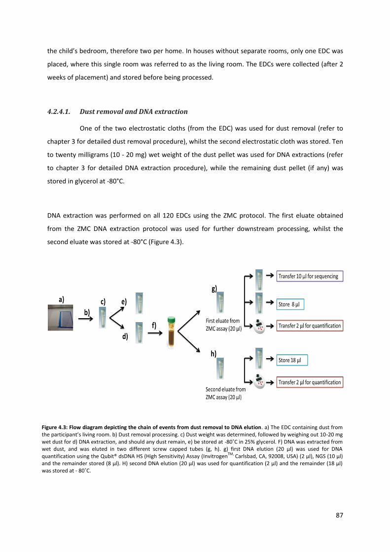
87

the child’s bedroom, therefore two per home. In houses without separate rooms, only one EDC was

placed, where this single room was referred to as the living room. The EDCs were collected (after 2

weeks of placement) and stored before being processed.

4.2.4.1. Dust removal and DNA extraction

One of the two electrostatic cloths (from the EDC) was used for dust removal (refer to

chapter 3 for detailed dust removal procedure), whilst the second electrostatic cloth was stored. Ten

to twenty milligrams (10 - 20 mg) wet weight of the dust pellet was used for DNA extractions (refer

to chapter 3 for detailed DNA extraction procedure), while the remaining dust pellet (if any) was

stored in glycerol at -80°C.

DNA extraction was performed on all 120 EDCs using the ZMC protocol. The first eluate obtained

from the ZMC DNA extraction protocol was used for further downstream processing, whilst the

second eluate was stored at -80°C (Figure 4.3).

Figure 4.3: Flow diagram depicting the chain of events from dust removal to DNA elution. a) The EDC containing dust from the participant’s living room. b) Dust removal processing. c) Dust weight was determined, followed by weighing out 10-20 mg wet dust for d) DNA extraction, and should any dust remain, e) be stored at -80˚C in 25% glycerol. F) DNA was extracted from wet dust, and was eluted in two different screw capped tubes (g, h). g) first DNA elution (20 µl) was used for DNA quantification using the Qubit® dsDNA HS (High Sensitivity) Assay (Invitrogen

TM, Carlsbad, CA, 92008, USA) (2 µl), NGS (10 µl)

and the remainder stored (8 µl). H) second DNA elution (20 µl) was used for quantification (2 µl) and the remainder (18 µl) was stored at - 80˚C.

88

4.2.4.1.1. DNA quantification

Each of the DNA samples were quantified with the Qubit® dsDNA HS (High Sensitivity)

Assay (InvitrogenTM, Carlsbad, CA, 92008, USA), using 2 µl genomic DNA. This dsDNA HS assay, allows

for the detection of only double stranded (ds) DNA, and is designed to be accurate for starting

concentrations of samples from 10 pg/µl to 100 ng/µl, therefore allowing for sensitive and accurate

detection of NA present within a sample. Once the samples had been quantified, 10 µl of genomic

DNA was aliquoted and sent to the J Craig Venter Institute (JCVI) (Maryland, USA) for NGS. JCVI is a

multidisciplinary genomic-focussed organisation. Due to UCT not having the capacity for

metagenomics studies, a collaboration was drafted with JCVI. As part of the collaboration of UCT

with JCVI, the division of Medical Microbiology participated in an exchange program with the aim of

local capacity building.

4.2.5. 16S rRNA amplicon Library preparation

The sequence of events for 16S rRNA amplicon preparation is outlined in Figure 4.4. All of

the steps were performed at JCVI (Refer to Appendix F for detailed description of the methods

involved).

Figure 4.4: Flow diagram representing the sequence of events for 16S rRNA amplicon preparation

89

A total of n=192 dust samples were sequenced on the Illumina MiSeq sequencer. Included in these

dust samples were 120 DCHS samples (comprising 60 pairs); 6 “sterile” EDCs from chapter 3 (5 of

which were sequenced in duplicate), 2 BEI controls (these controls contain genomic DNA from 20

bacterial strains, and are therefore used as a control for a metagenomics sample), 1 E.coli control

and1 no-template Control (Table 4.1).

Sample Type Sample amount (n=)

Sequenced in duplicate (n=)

DCHS EDC samples 120 10 Sterile EDC controls 6 5

Dust other 25 22

BEI controls 2 0 E.coli control 1 0

No-template Control 1 0

Total 155 37

4.2.6. Running of the 16S rRNA YAP pipeline

The bioinformatic analysis was performed in collaboration with JCVI (J Craig Venter

Institute), Maryland, USA as well as with the Computational Biology group at the University of Cape

Town. The bioinformatics pipeline known as ”Yet Another Pipeline” (YAP) (Szpakowski, 2013) was

downloaded from GitHub, and used to classify 16S rRNA sequences into bacterial taxonomies. YAP

consists of a custom python wrapper that meshes a set of tools integrated into a computationally

efficient workflow, depicted in Figure 4.5 (A detailed explanation of the YAP pipeline is described in

Appendix G).

Table 4.1: Summary of the number and sample types that were sequenced

90

Figure 4.5: Summary of the bioinformatics steps included in the YAP pipeline

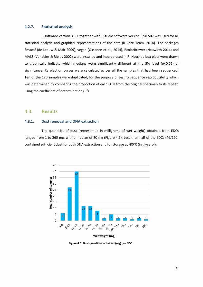
91

4.2.7. Statistical analysis

R software version 3.1.1 together with RStudio software version 0.98.507 was used for all

statistical analysis and graphical representations of the data (R Core Team, 2014). The packages

Smacof (de Leeuw & Mair 2009), vegan (Oksanen et al., 2014), RcolorBrewer (Neuwirth 2014) and

MASS (Venables & Ripley 2002) were installed and incorporated in R. Notched box plots were drawn

to graphically indicate which medians were significantly different at the 5% level (p<0.05) of

significance. Rarefaction curves were calculated across all the samples that had been sequenced.

Ten of the 120 samples were duplicated, for the purpose of testing sequence reproducibility which

was determined by comparing the proportion of each OTU from the original specimen to its repeat,

using the coefficient of determination (R2).

4.3. Results

4.3.1. Dust removal and DNA extraction

The quantities of dust (represented in milligrams of wet weight) obtained from EDCs

ranged from 1 to 260 mg, with a median of 20 mg (Figure 4.6). Less than half of the EDCs (46/120)

contained sufficient dust for both DNA extraction and for storage at -80˚C (in glycerol).

Figure 4.6: Dust quantities obtained (mg) per EDC.

92

DNA extractions from ≤ 10 mg of wet dust from the 120 EDC’s, yielded DNA concentrations from 0

to 12.4 ng/µl (Figure 4.7), with a median of 1.32.

The 120 dust samples were divided into four groups based upon the season in which they were

collected. Total DNA yield for the dust samples within each season is represented by notched box

plots (Figure 4.8). All notches (across the seasons) overlap, indicating no significant difference

between the medians at a 5% significance level. However, the range for spring is greater than the

range across the other seasons.

Figure 4.7: DNA concentrations (ng/µl) obtained for each of the 120 EDCs

Figure 4.8: Box plot representing the DNA yield (ng/µl), according to season. The box represents the Inter Quartile Range (IQR), which extends from the 75

th to the 25

th percentile. The whiskers extend 75

th percentile by 1.5 times

the IQR, and the 25th

percentile by -1.5 times the IQR. The line represents the median of the data, and the notch is indicative of the confidence interval around the median.

93

The 120 dust samples were collected as 60 paired samples. Dust was sampled from the same homes

approximately six months apart. These two sampling times were referred to as placement 1 and

placement 2. Dividing the dust samples into 2 groups (to represent the 2 placement times), and then

comparing the DNA yields between the placements, showed no marked differences between the

notched box plots (Figure 4.9).

4.3.2. Summary statistics on the data metrics obtained from the Illumina MiSeq

sequencer software and the 16S YAP workflow for all sampling groups

A total of n=192 samples were sequenced on the Illumina MiSeq sequencer. An indication

of a successful NGS run is measured by the raw clusters per lane. In this study, the raw clusters per

lane ranged from 0.02 to 0.86%. A total of 68 124 OTUs were observed across all the samples.

A total of 3,63 Gb of total yield was obtained for this run. The Illumina sequencing platforms

removes low quality clusters (i.e., reads) using the Illumina chastity filter

(http://support.illumina.com/sequencing/sequencing_instruments/hiseq_2500/questions.html).

This filter step occurs before generating the resultant files (e.g., FASTQ files). A total of 12 783 482

reads (raw sequences) passed the filter, with an average of 66 580 reads per sample prior to

demultiplexing. A mean Q-score of 31.14 was obtained per sample.

Figure 4.9: Box plot representing the DNA yield (ng/µl), according to placement. The box represents the Inter Quartile Range (IQR), which extends from the 75

th to the 25

th percentile. The whiskers extend 75

th percentile by 1.5 times the IQR,

and the 25th

percentile by -1.5 times the IQR. The line represents the median of the data, and the notch is indicative of the confidence interval around the median.

94

The number of reads decreased by 60% after the de-multiplexing and quality trimming step (from

12 783 482 raw reads to 5 118 272, Table 4.2). The sequencing reads decreased by 32% after

ambiguous bases were removed (Table 4.2, Step 2). A further 15% decrease in sequencing reads

occurred after chimeric sequences were removed (Table 4.2, step 5). A total of 2 962 017 reads

remained at the end of the YAP pipeline, with an average of 15 507, 94 reads per sample.

4.3.2.1. Summary statistics on the data metrics obtained from the Illumina MiSeq

sequencer software and the 16S YAP workflow for all sampling groups, based on

season

No significant difference could be observed when comparing the mean quality scores

between the seasons (Figure 4.10). Across all four seasons the Q-score was >31.

Step based on Figure 4.5

Description Total number of

reads

Average number of reads per

sample

1. Sequences that remain after demultiplexing and quality trimming. 5 118 272 26 797.24

2. The sequences with ambiguous bases were filtered out, only the

sequences that are 220 – 250 bases in length, remained.

3 466 092 18 147.08

3. Unique sequence remained, and the duplicates were collapsed. 3 466 092 18 147.08

4. Unique sequences that aligned against a database of 16S rDNA

sequences remained.

3 466 092 18 147.08

5. Chimeric sequences removed, bad alignments removed, the

sequences outside primer range clipped, and erroneous, misaligned

sequences filtered out

2 962 017 15 507.94

6. The final sequence counts, based on the sequence / similarity

clustering

2 962 017 15 507.94

Table 4.2: Total Number of reads obtained per sequencing step, with the average number of reads per sample per output step.

Figure 4.10: Notched box plots, representing the Mean Quality Scores according to seasons. The box represents the Inter Quartile Range (IQR), which extends from the 75

th to the 25

th percentile. The whiskers extend 75

th

percentile by 1.5 time the IQR, and the 25th

percentile by -1.5 times the IQR. The line represents the median of the data, and the notch is indicative of the confidence interval around the median.

95

4.3.2.2. Summary statistics on the data metrics obtained from the Illumina MiSeq

sequencer software and the 16S YAP workflow for all sampling groups, based on

placement

Once again, no significant differences could be observed for the mean quality scores

obtained between placements one and two. In both cases, the Q-score was >32 (Figure 4.11).

4.3.2.3. Summary statistics –Rarefaction curves

In metagenomic studies, more diverse samples require a higher number of reads to be

fully characterised. When observing the rarefaction curves, approximately half of the samples had

reached plateau phase, indicating sufficient sequencing depth. However, rarefaction curves for the

remainder of the samples indicated insufficient sequencing depth to characterise these remaining

bacterial genera (Figure 4.12).

Figure 4.11: Notched box plots, representing the Mean quality score according to placements. The box represents the Inter Quartile Range (IQR), which extends from the 75

th to the 25

th percentile. The whiskers extend 75

th percentile by 1.5

times the IQR, and the 25th

percentile by -1.5 times the IQR. The line represents the median of the data, and the notch is indicative of the confidence interval around the median.

Figure 4.12: Rarefaction curves of high throughput sequencing of the V4 region of the 16S rRNA gene.

96

4.3.2.4. Summary statistics –Reproducibility between duplicate sequenced samples

By fitting the regression line, the R2 value indicated how closely the samples match to

their duplicate samples. From Figure 4.13, the variation between the technical repeats is indicated

as an R2 value of 0.94, and is considered as high reproducibility between the duplicate samples.

4.3.2.5. Summary statistics for the Sterile EDCs and Non template control

The average number of sequences per sterile EDC before and after the YAP pipeline were

77732, and 5256 reads respectively, resulting in a proportional decrease of 93%. The no-template

control that was included in the sequencing run had 218 080 reads before and 72 reads after going

through the YAP pipeline, resulting in proportional decrease of 99.96%.

Figure 4.13: Regression line indicating the reproducibility between the duplicate samples. Further away from the regression line, indicates increased difference between the duplicates. A theoretical value of 1.00 indicates that everything is exactly the same between duplicates. The sizes of the squares indicate the reproducibility between the samples. The bigger the block the lower the reproducibility between sample and its duplicate, and vise versa. Each colour represents a different level of DNA yield. The more red, the lower the yield, the more green, the higher the yield. Additionally, every square indicated in the figure is a representative of a taxanomic unit.

97

4.4. Discussion

NGS is a non-biased way to identify all the bacteria that are present within a sample. The

use of Illumina sequencing allows for identification and determination of unknown as well as non-

culturable bacteria; it is reproducible; allows for phylogenetic identification, it is fast, makes use of

short reads, and it circumvents homopolymer issues (which are a downfall for certain other

sequencing technologies). However, a limitation to this type of technique is that data analysis is

computationally intense (Fraher et al., 2012).

Prior to sequencing, dust was removed from the EDCs, where the wet weights obtained from the

EDCs were variable, with the lowest quantities being between 1 and 5 mg. These samples were also

included in the sequencing run, even though they yielded less than 10 mg of starting wet weight.

This variability in dust weight removed from the EDCs could be: 1) due to the loss of sample during

the dust removal process, where dust particles may have stayed behind and not detached from the

EDCs; and 2) due to the fact that the EDCs were placed in different households, and therefore would

have had varying amounts of dust.

DNA yields obtained from the dust samples decreased across the seasons, with spring having the

highest DNA yield, followed by summer, autumn and winter (which had the lowest DNA yield).

Studies have shown that variation in the DNA yields that are used for library preparation may impact

on the variability of the sequencing results (Gutiérrez et al., 2014; Kennedy et al., 2014).

In comparison to 454 pyrosequencers, the Illumina platform has increased throughput per run,

which allows for deeper sequencing of the multiplexed samples (Glenn 2012). The sequencing depth

represents the number of times each base is sequenced, and is dependent on the throughput of the

specific instrument, the size of the template and the number of samples per run. Illumina also

contains a robust paired-end sequencing technology that is capable of sequencing a DNA template

from both ends (Eren et al., 2013). Illumina reads rely on machine generated Q-scores for quality

filtering (Minoche et al., 2011; Bokulich et al., 2013).

Q scores indicate the probability that a base is called incorrectly by the sequencer. It is generally

observed that for Illumina runs Q-scores are in the mid-thirties at the start of the reads, and

gradually decline towards the end of the reads. A Q-score of 30 indicates base call accuracy of

98

99.99% and is considered the benchmark for quality in next-generation sequencing (Ewing & Green

1998; Ewing et al., 1998). Therefore, a mean Q-score of 31.14 (17.74; 33.34) per sample (obtained in

this study) would be considered as acceptable.

Q-score-based quality filtering methods rely on Phred like algorithms to determine the accuracy of

base calls (Ewing & Green, 1998a; Ewing et al., 1998b) . Q-score thresholds allow successful removal

of low quality reads. Eren et al., (2013) demonstrated that methods which rely on machine

generated Q-scores may over-estimate the overall accuracy. Eren et al., (2013) compared the

overlap of paired-end, short sequence reads (to obtain sequence consensus or to identify error-

prone reads) to sequences that relied on Q scores generated by the sequencer (Minoche et al., 2011;

Bokulich et al., 2013). The number of clusters which were identified within the reads that were

filtered with the paired-end overlap method had approximately 30% fewer clusters than those

identified in the reads that were filtered based on the Q-score based methods (Minoche et al., 2011;

Bokulich et al., 2013). Therefore, Q score methods may include low quality reads, containing

sequencing errors, resulting in misleading overall accuracy (Eren et al., 2013). Studies conducted

using Pyrosequencing, have identified an increase in diversity estimates and richness that are caused

by low quality reads (Quince et al., 2009; Kunin 2010).

No significant differences were observed between the mean quality scores obtained for the different

seasons (Figure 4.10). Similarly, no significant differences were observed between the mean quality

scores obtained for the two placement times (Figure 4.11).

Sequencing reads were obtained in all six EDC’s that were considered sterile (that is, free from

micro-organisms), as well as in the no-template controls. As previously mentioned in chapter 3, UVGI

seemed effective in rendering the micro-organisms as non-culturable. However, UVGI did not

remove the non-culturable micro-organisms from the EDC. It is possible that these non-culturable

micro-organisms were removed with the dust from the EDCs. NGS is a highly sensitive technique,

and it is therefore likely that the V4 region of the non-culturable bacteria were undamaged by UVGI,

therefore, allowing sequencing and identification of these non-culturable bacteria from the sterile

EDCs. The sterile EDCs and the no-template controls contained at least 66% and 99.5% fewer reads

respectively when compared to the rest of the EDC samples.

99

Second generation technologies are susceptible to contamination (Langdon 2014), due to the fact

that they are amplification based technologies (Aslanzadeh 2004). A number of reasons may be

attributed to the reads generated for the no-template control, such as well-to-well contamination.

Other sources of possible contamination include: 1) the type of molecular PCR grade water (Nogami

et al., 1998; Shen et al., 2006; Bohus et al., 2011;), 2) DNA extraction kits (Mohammadi et al., 2005)

and 3) PCR reagents (Grahn et al., 2003). Cross contamination, may result in false-positive PCR

products and inevitably a false representation of bacterial diversity both between as well as within

samples, thereby affecting data analysis.

A way in which species diversity can be measured is with the use of rarefaction or species

accumulation curves. These curves indicate how well a sample was characterised based on

estimated sample diversity and sequencing depth (Wooley et al., 2010), and are commonly used to

describe species richness (Brodie et al., 2007; Gotelli & Colwell, 2009; Hamady & Knight, 2009; Abed

et al., 2012; Kembel et al., 2012(b); Yamaguchi et al., 2012). When more genera are present within a

sample, increasing sequencing depth is required to fully characterise a sample. The slope of the

curve decreases until it plateaus. When the plateau state is reached increasing sequencing depth will

not add significantly more species being detected (Gotelli & Colwell 2001). However, should the

plateau not be reached, as is the case for half of the samples sequenced (Figure 4.12), increased

sequencing depth would have increased the probability of finding more genera within that specific

sample. It is most likely that only the more abundant genera have been identified for these samples,

meaning that the remainder of the genera have not been identified using this form of sequencing.

Therefore, the sequencing depth obtained for the dust samples, could be considered as variable, as

half of them had reached their plateau state, whilst the other half were still on the rise.

Reproducibility was determined by comparing the proportion of each OTU from the original

specimen to its repeat, using the coefficient of determination (R2). The variation between technical

repeats was calculated at R2 = 0.94. The overall reproducibility was good, considering 1) the overall

reproducibility was tested between two repeats only, and 2) the high variation for amplicon-based

sequencing approaches. The poor reproducibility obtained for certain samples, included samples

with both low and high DNA yields (depicted by orange/red and green squares, Figure 4.13).

Therefore DNA yield does not seem to influence reproducibility.

100

4.5. Conclusion

A total of 2 962 017 reads were obtained across the 192 samples that were sequenced,

after processing through the YAP pipeline. Based on the results, it is evident that good

reproducibility was obtained for the sequencing run, together with good quality reads. Furthermore,

the low DNA yields that were obtained from each of the samples, did not seem to have an influence

on the reproducibility of the sequencing run. However, the depth of sequencing for this run can be

considered as variable, and therefore deeper sequencing would be needed to fully characterise the

remaining half of the samples. No significant findings could be drawn in relation to DNA yield and or

number of reads according to season or placement. Reads observed in the NTC is an indication of

low level contamination, as it accounted for only 0.05% when compared to the number of reads

obtained per DCHS dust sample. Reads were observed in the sterile controls, and need to be

accounted for prior to further data analysis.

101

CHAPTER 5

Pilot Study Data Analysis

102

CHAPTER 5: Pilot Study Data Analysis The output of the YAP pipeline was an Operational Taxonomic Unit (OTU) table. This chapter

describes the analysis of data in this table to improve our understanding of the microbial

composition of house dust, and the influence that season and other contributing factors may have

on the house dust microbiome.

5.1. Aims

The aims of the analysis described in this chapter are to:

1) Identify the bacterial genera found within the “sterile” EDCs, and to correct for these in the placed

EDCs in order to allow further analysis.

2) Describe the bacterial microbiome present within house dust samples, specifically to address the

following questions:

- Do seasons have an effect on the indoor microbiome?

-Do pets, number of occupants as well as room size have an effect on the indoor

microbiome?

- Does geographic location, as well as ventilation influence the indoor microbiome?

5.2. Statistical Analysis methods

R software version 3.1.1 together with RStudio software version 0.98.507 was used for all

statistical analysis and graphical representations of the data (R Core Team 2014). The packages

Smacof (de Leeuw & Mair 2009), vegan (Oksanen et al., 2014), RcolorBrewer (Neuwirth 2014) and

MASS (Venables & Ripley 2002) were installed and incorporated in R. Based on 97% sequence

similarity, the pre-processed sequences were assigned to Operational Taxonomic Units (OTU).

5.2.1. Accounting for OTUs found in the sterile EDCs

The average proportions of genus-level OTUs were calculated in the sterile EDCs and

compared to the OTUs present within the dust samples. A barplot was used to compare the genera

found in the sterile samples, alongside the same genera found in the dust samples.

103

To correct for the OTUs present in the sterile EDCs, the following approach was taken:

1) The mean number of OTUs from the sterile EDCs was collected for each taxon where

contamination was observed.

2) The mean of each of the OTUs representing the contamination was subtracted from each of the

corresponding specimen OTUs.

3) The resultant number of OTUs at the genus level was added together to obtain the new number

of OTUs at the family level. This was then added to obtain the new number of OTUs at the order

level. This was continued until the root was reached.

Scaled deviations were calculated for each genus by dividing the deviation from the mean by the

standard deviation. Some of the genera found in the sterile EDC controls had scaled deviations >0.5.

This can be viewed as contamination of the samples (sterile EDC and dust samples), since the

abundance observed in the sterile EDCs are >0.5 standard deviations larger than the mean. To

correct for this, the method outlined above is used. When performing the correction, all the genera

found in the sterile EDCs are considered, not only those with scaled deviations >0.5.

Box plots were used to compare the most abundant genera found in the EDCs before and after

accounting for the “contamination” amongst all the samples.

5.2.2. Measuring Diversity

Alpha (α) as well as Beta (β) diversity was calculated to measure the diversity within and

between the samples, respectively. Beta diversity is defined as a measure of the difference in species

composition between samples/communities (Sfenthourakis & Panitsa 2012). Alpha diversity is

defined as the diversity of a species within a local community, habitat or sample (Gotelli & Colwell

2009).

5.2.2.1. Shannon diversity

As a measure of α-diversity, the Shannon diversity index was used to measure both

richness as well as evenness within a sample. Where:

H= - ∑ 𝑃𝑖𝑠𝑖=1 ln 𝑝𝑖

104

where:

∑ = represents the sum from species 1 to species S

S = represents the numbers of species that were encountered

H = represents the Shannon diversity index

Pi = represents the fraction of the entire population made up of species i

Box plots were used to graphically represent the Shannon diversity. The Shannon diversity was

compared between the different seasons, the number of occupants, pets, rooms within a household,

whether or not the windows were open or closed during placement, and between the two different

regions in Paarl (TC Newman and Mbekweni).

5.2.2.2. Barplots

5.2.2.2.1. Bray-Curtis Dissimilarity Index

The Bray-Curtis dissimilarity index is used to quantify the compositional dissimilarity

between two different sites, based on counts present at each site (Morgan & Huttenhower 2012).

We used the Bray-Curtis dissimilarity index to calculate the difference between the samples. From

the help file of the function vegdist in R package vegan (Oksanen et al., 2014), the following was

obtained:

𝐵𝐶𝑗𝑘 =∑ |𝑥𝑖𝑗 − 𝑥𝑖𝑘|𝑆

𝑖=1

∑ (𝑥𝑖𝑗 + 𝑥𝑖𝑘)𝑆𝑖=1

Where:

∑ represents the sum from species 1 to species 𝑆

𝑆 represents the number of species that were encountered

𝑗, 𝑘 represent the two samples between which the dissimilarity is calculated

𝑥𝑖𝑗 is the abundance of species 𝑖 in sample 𝑗

𝑥𝑖𝑘 is the abundance of species 𝑖 in sample 𝑘

| | indicates the absolute value (Faith et al., 1987)

The Bray-Curtis distance is a value between 0 and 1, where 0 indicates that the samples are identical

and 1 means that they are completely different. The distances between pairs of samples were

calculated in this way.

105

5.2.2.2.2. Complete linkage of hierarchical clustering

Complete linkage hierarchical clustering was performed on all of the samples according

to Hair et al., (2006). The following approach was taken: 1) each sample was identified as a cluster

on its own, then 2) the two closest clusters were merged together (this is where Bray-Curtis

dissimilarity index was used) and 3) the new distance between each of the other clusters and the

new merged cluster was calculated. With the complete linkage algorithm, this amounts to selecting

the largest pairwise distance between elements of the two clusters to represent the inter-cluster

distance. 4) Steps 2 and 3 were then repeated in order to merge all of the samples into a single

cluster. This process was then graphically illustrated by a clustering tree, showing the sequence of

mergers. Actual clustering was then performed on the tree, by horizontally cutting through the tree,

everything that merged above, became a separate cluster. Mergers above the cutting threshold

were not considered, forming separate clusters.

The bars in the barplots correspond to the samples in the clustering tree. The majority of bar plots

are depicted at class level in order to illustrate a neater and uncluttered representation of the

bacteria present within the dust samples. As a means to observe if there were any specific

characteristics that correspond with clustering, a line with coloured blocks was plotted at the

bottom of each of the clustering trees. Several characteristics were chosen, such as type of home,

region of EDC placement, season etc., each of which were indicated by colour-coded squares.

5.2.2.2.3. Multidimensional scaling plots

In order to compare the different clusters, the mean proportion of each OTU was

calculated for each cluster. A pie chart was used to represent each cluster. Multidimensional Scaling

plots (MDS) (a two-dimensional display that represents dissimilarities between the clusters) were

used in order to show that pie charts further away, are less similar than pie charts that were situated

closer together. In our case, the Bray-Curtis index was used in order to determine the distance

between each of the pairs of clusters. The algorithm SMACOF (Majorising a Complicated Function)

was also used to obtain the MDS plot (Borg & Groenen 2005). The labelling of the clusters

corresponds with the order in the clustering tree. This visual analysis was performed at class level.

The clustering was performed on the datasets with OTUs where the abundance was >0.5%.

106

OTUs with abundance <0.5% were not clustered separately. These OTUs are represented in bar plots

and the MDS plots are based on the corresponding clusters formed with the OTUs with abundance

>0.5%. Additionally, relative abundance was expressed at the phylum level.

5.2.2.3. Biplots

In order to understand whether the indoor microbial composition was influenced by

external factors, such as time of placement and season, biplots were constructed. Biplots are

exploratory graphs used in statistics. In our case, the length of the linear line between placement

one and placement two would indicate how closely related the bacterial clusters (between

placement one and placement two, within the same household) are to one another. The longer the

length the further away the clusters are between the placements and therefore the less similar the

sequences obtained between one another. The Bayesian prior technique of Fernandes et al., (2011)

was used (equation 4.6, with perks prior to table 4.2 in Fernandes et al., (2011)). Lambda scaling was

also implemented to generate the biplot (section 2.3.1 in Gower et al., 2010).

5.2.2.4. Generalised Linear Mixed Models

The generalised linear model (GLM) makes provision for count data. Since sequencing

data are compositional (Fernandes et al., 2014), the total number of OTUs found in each sample

needed to be taken into account. This is included in the GLM with an offset argument which equals

the OTU count at root level.

In this analysis, the same household was measured at placements ‘1’ and ‘2’. With repeated

measures, the observations from the two placements in the same household was not independent

and a further generalisation called GLMM is needed (Cnaan et al., 1997). The GLMM was

implemented in R with the function glmmPQL from package MASS (Venables & Ripley 2002).

Once the model was fitted with the glmmPQL function, the expected proportion of the particular

OTU was obtained from the model, �̂�. Interpretation of the model coefficients was performed in

terms of the rate ratio:

�̂�𝑠𝑝𝑟𝑖𝑛𝑔

�̂�𝑤𝑖𝑛𝑡𝑒𝑟= 𝑅𝑅(𝑠𝑝𝑟𝑖𝑛𝑔 𝑣𝑠 𝑤𝑖𝑛𝑡𝑒𝑟)

107

This means �̂�𝑠𝑝𝑟𝑖𝑛𝑔 = 𝑅𝑅 × �̂�𝑤𝑖𝑛𝑡𝑒𝑟. Say the rate ratio was 𝑅𝑅 = 1.2, this would mean that

�̂�𝑠𝑝𝑟𝑖𝑛𝑔 = 1.2 × �̂�𝑤𝑖𝑛𝑡𝑒𝑟

which was interpreted as the proportion of this OTU in spring was 1.2 times as much as the

proportion of the same OTU in winter, i.e., there was a 20% increase in spring. On the other hand, if

𝑅𝑅 = 0.5 then

�̂�𝑠𝑝𝑟𝑖𝑛𝑔 = 0.5 × �̂�𝑤𝑖𝑛𝑡𝑒𝑟

and the proportion of this OTU in spring was only half as much as in winter.

In the analyses, GLMM models where fitted for each OTU with an overall abundance of >0.5%. The

models included seasons, and house types, therefore the hypotheses being tested are given by 𝐻0:

the proportion of this OTU is the same for all seasons vs the alternative hypotheses 𝐻𝑎: the

proportion of this OTU is different between at least two of the seasons and 𝐻0: the proportion of

this OTU is the same for all house types vs the alternative hypotheses 𝐻𝑎: the proportion of this OTU

is different between at least two of the house types.

For each variable considered (season and house type), a t-test was performed to test the statistical

significance of that variable in the model. Testing this for each OTU meant that thousands of t-tests

were performed. Benjamini and Hochberg (1995) suggest an adjustment to the p-values to control

the false discovery rate. The adjusted p-values less than 0.05 were considered statistically significant

(Benjamini & Hochberg 1995).

Winter was used as the reference for season; house was used as the reference for type of home; and

no pets was used as the reference for homes with or without pets.

5.3. Results

Clustering the unique sequences into OTUs at 97% sequence similarity level, resulted in

308 789 different OTUs across the 142 samples (including the sterile samples, sequencing duplicates,

and no-template control). These OTUs spanned 1233 genera including 337 families, 149 Orders, 83

Classes and 35 phyla. Furthermore, these sequences also covered four domains, namely: Archaea

(124); bacteria (308588), unclassified (4) and unknown (73). Unclassified refers to bacterial OTUs

108

that could not be classified to a genus, and unknown refers to OTUs that could not be classified to

either eukarya, archaea or bacteria.

5.3.1. Genera present in the no-template control and sterile EDC controls

The no-template control (NTC) was included at the library preparation step and was

processed along with the dust samples. The NTC contained water instead of template DNA and

represents a negative control for the sequencing run. However, 37 different OTUs were identified in

the no-template control. Twenty of which corresponded to the phylum Proteobacteria, and nine to

the phylum Actinobacteria. The relative abundance of these phyla identified in the no-template

control was extremely low when compared to the relative abundance of these phyla in the dust

samples. Correction for the NTC made no impact on the analysis of the rest of the dust samples.

Furthermore, correcting for the sterile EDCs (below) reduced all OTUs from the NTC to zero.

A total of 200 genera belonging to 25 of the 35 bacterial Phyla were identified in the sterile controls.

When the genus OTUs in the sterile samples (Figure 5.1A) were compared to the genus OTUs

present in the dust samples in Figure (5.1B), the white spaces indicate the genera not found within

the dust samples.

Figure 5.1: Pie chart indicating A) the proportion of genera identified in the sterile EDCs and B) the same genera identified in the sterile EDCs and in the dust samples. The arrows are indicating the genera found in the sterile EDCs only and not in the dust samples.

109

The white spaces in Figure 5.1B represent 13 Genera, 2 of which belonged to the domain Archeae

(Table 5.1). Most (11/13) of the genera that were identified in these sterile EDCs, belong to the phyla

Proteobacteria.

Genus Family Order Class Phylum Domain Methanocorpusculum Methanocorpusculaceae Methanomicrobiale

s Methanomicrobia Euryarchaeota Archaea

Unclassified Unclassified Thermoplasmatales Thermoplasmata Euryarchaeota Archaea

Hydrogenobacter Aquificaceae Aquificales Aquificae Nitrospira Bacteria

Bradyrhizobium Bradyrhizobiaceae Rhizobiales Alpha Proteobacteria Proteobacteria Bacteria Novispirillum Rhodospirillaceae Rhodospirillales Alpha Proteobacteria Proteobacteria Bacteria Unclassified Rickettsiaceae Rickettsiales Alpha Proteobacteria Proteobacteria Bacteria

Polynucleobacte Burkholderia Burkholderiales Beta Proteobacteria Proteobacteria Bacteria Tepidimonas Burkholderiales_incertae_sedis Burkholderiales Beta Proteobacteria Proteobacteria Bacteria Curvibacter Comamonadaceae Burkholderiales Beta Proteobacteria Proteobacteria Bacteria Diaphorobacter Comamonadaceae Burkholderiales Beta Proteobacteria Proteobacteria Bacteria

Hydrogenophilus Hydrogenophilaceae Hydrogenophilales Beta Proteobacteria Proteobacteria Bacteria Thiobacillus Hydrogenophilaceae Hydrogenophilales Beta Proteobacteria Proteobacteria Bacteria Shewanella Shewanellaceae Alteromonadales Gamma Proteobacteria Proteobacteria Bacteria

A bar plot was used to graphically compare the genera observed in the sterile samples to the same

genera observed in the dust samples (Figure 5.2). Each bar represents a sample, with different

colours representing different genera. The height of the bar indicates the OTU counts for that

sample. When comparing the OTU counts of the sterile samples to that of the dust samples, it is

evident that the sterile samples contain approximately 10% of the OTU counts of the same genera

found in the dust samples, therefore indicating that there are more reads and thus more of these

genera present in the dust samples than in the sterile controls.

Table 5.1: Table indicating the different taxonomic levels of the 13 genera that were identified in the sterile samples only

110

Figure 5.2: Barplot representing the OTU counts of genera in the sterile EDCs and dust samples.

111

Figure 5.3: Colour key for Figure 5.2.

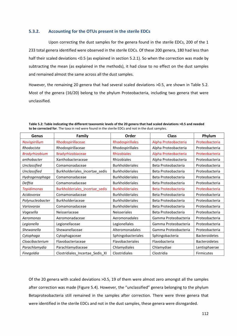
112

5.3.2. Accounting for the OTUs present in the sterile EDCs

Upon correcting the dust samples for the genera found in the sterile EDCs, 200 of the 1

233 total genera identified were observed in the sterile EDCs. Of these 200 genera, 180 had less than

half their scaled deviations <0.5 (as explained in section 5.2.1). So when the correction was made by

subtracting the mean (as explained in the methods), it had close to no effect on the dust samples

and remained almost the same across all the dust samples.

However, the remaining 20 genera that had several scaled deviations >0.5, are shown in Table 5.2.

Most of the genera (16/20) belong to the phylum Proteobacteria, including two genera that were

unclassified.

Genus Family Order Class Phylum Novispirillum Rhodospirillaceae Rhodospirillales Alpha Proteobacteria Proteobacteria

Rhodocista Rhodospirillaceae Rhodospirillales Alpha Proteobacteria Proteobacteria

Bradyrhizobium Bradyrhizobiaceae Rhizobiales Alpha Proteobacteria Proteobacteria

anthobacter Xanthobacteraceae Rhizobiales Alpha Proteobacteria Proteobacteria

Unclassified Comamonadaceae Burkholderiales Beta Proteobacteria Proteobacteria

Unclassified Burkholderiales_incertae_sedis Burkholderiales Beta Proteobacteria Proteobacteria

Hydrogenophaga Comamonadaceae Burkholderiales Beta Proteobacteria Proteobacteria

Delftia Comamonadaceae Burkholderiales Beta Proteobacteria Proteobacteria

Tepidimonas Burkholderiales_incertae_sedis Burkholderiales Beta Proteobacteria Proteobacteria

Acidovorax Comamonadaceae Burkholderiales Beta Proteobacteria Proteobacteria

Polynucleobacter Burkholderiaceae Burkholderiales Beta Proteobacteria Proteobacteria

Variovorax Comamonadaceae Burkholderiales Beta Proteobacteria Proteobacteria

Vogesella Neisseriaceae Neisseriales Beta Proteobacteria Proteobacteria

Aeromonas Aeromonadaceae Aeromonadales Gamma Proteobacteria Proteobacteria

Legionella Legionellaceae Legionellales Gamma Proteobacteria Proteobacteria

Shewanella Shewanellaceae Alteromonadales Gamma Proteobacteria Proteobacteria

Cytophaga Cytophagaceae Sphingobacteriales Sphingobacteria Bacteroidetes

Cloacibacterium Flavobacteriaceae Flavobacteriales Flavobacteria Bacteroidetes

Parachlamydia Parachlamydiaceae Chlamydiales Chlamydiae Lentisphaerae

Finegoldia Clostridiales_Incertae_Sedis_XI Clostridiales Clostridia Firmicutes

Of the 20 genera with scaled deviations >0.5, 19 of them were almost zero amongst all the samples

after correction was made (Figure 5.4). However, the “unclassified” genera belonging to the phylum

Betaproteobacteria still remained in the samples after correction. There were three genera that

were identified in the sterile EDCs and not in the dust samples, these genera were disregarded.

Table 5.2: Table indicating the different taxonomic levels of the 20 genera that had scaled deviations >0.5 and needed to be corrected for. The taxa in red were found in the sterile EDCs and not in the dust samples.

113

5.3.3. House dust microbiome

After correcting for the taxa observed in the sterile EDCs, the different classes of bacteria

present within the 120 house dust samples were represented as a barplot (Figures 5.5). The less

abundant classes with a relative abundance of <0.5%, were included in the above bar plot and are

represented as “other” in grey.

Actinobacterium was the predominant phylum in house dust samples, followed by Proteobacterium

and then Firmicutes (which includes Clostridium and Bacillus) (Figure 5.5). A few households showed

a larger abundance in Bacteroidia (Figure 5.5).

The lower abundant bacterial classes (depicted as in grey as “other” in Figure 5.5) are shown in

greater detail in Figure 5.6. Of the less abundant classes, the most prevalent class is a member of the

phylum Acidobacteria. Some households had noticeably more classes of “unclassified” bacteria (in

purple) than other households.

Figure 5.4: Box plots representing the 20 genera with scaled deviations >0.5. A) Before and B) after the correction was made.

114

Figure 5.5: Representation of all the taxa, at class level across the 120 dust samples: A) Cluster dendogram corresponding to the dust samples. The red squares in the cluster dendogram indicate the different clusters in the tree. B) Represents the different characteristics that may influence the house dust microbiome. C) Barplot representing the higher abundant taxa at class level across all 120 dust samples. The lower abundant taxa <0.5, are indicated in grey as “other”.

115

Figure 5.6: Barplot representing the lower abundant taxa (< 0.5) at class level across all 120 dust samples.

116

MDS plots in Figure 5.7 represent the distance between the different clusters (depicted in the

dendogram in Figure 5.5), as well as a simplified representation of the bacterial classes present

within that cluster (Figure 5.5 & 5.6). Therefore when studying the clusters assigned on the

dendogram concurrently with the MDS plots, it could be noted that clusters five and six were similar

to one another (Figure 5.7). Clusters five and six represent the most dust samples (Figure 5.5), and

contains the highest amount of Acidobacteria (Figure 5.7B). Cluster four represents nine samples

collected from the TC Newman region only (Figure 5.5). Cluster one contains the most Bacteroidetes

(Figure 5.7), and cluster two contains the most Firmicutes (Figure 5.7). Clusters one and two consist

of three and two samples respectively (Figure 5.5). Cluster three has the highest counts of

Proteobacteria OTUs (Figure 5.7A), as well as an “unclassified” phylum (Figure 5.7B).

Figure 5.7: Multidimensional scaling plot indicating A) the clusters that correspond all the taxa (Figure 5.5), and B) the clusters that correspond to the lower abundant taxa (depicted in grey as “other”; Figure 5.6)). See Figure 5.5 and 5.6 for colour key.

117

In the plots above (Figure 5.5 - 5.7), each sample point is considered separately. However, with two

placements per household, each household can be viewed as a unit with two sample points. This is

shown in Figure 5.8 below.

Figure 5.8 represents all the OTUs that were present in the dust samples, at class level across the

120 samples. As previously mentioned, the less abundant classes <0.5 are represented as “other” in

grey. The 60 EDC pairs are listed in this Figure, where placement 1 is situated below placement 2 in

order to make a visual comparison between the placements within the same household. The

dendogram (Figure 5.8) was constructed for this, where the dissimilarities were calculated between

each pair and summed according to Bray-Curtis.

118 Figure 5.8: Abundant taxa, at class level, across the 120 dust samples (separated into their pairs). Placement 1 = First placement, and Placement 2 = second placement. : A) Cluster dendogram corresponding to the

dust samples. The red squares indicate the different clusters in the tree. B) Possible external factors contributing to house dust diversity. C) Barplots representing the higher abundant taxa at class level, across all 120 dust samples.

A)

B)

N +-' c Q)

E Q) u ro

0....

C)

....-i +-' c Q)

E Q) u ro

0....

C)

~'W"tJ · P•U •

~ R•lkon •

~

!li

~

~

~

~

~

!li

~

~

~

Dust samples in pairs Number of occupants

House type

Pets Region

• • • • • • . . .

Key for 8

Key for C

other

1 unclassified

1 Clostridia

1 Bacilli Cyanobacteria

Chloroplast

1 unclassified 1 Gammaproteobacteria

1 Deltaproteobacteria

1 Betaproteobacteria

1 Alphaproteobacteria

I Planctomycetacia Gemmatimonadetes

1 Deinococci 1 Thermomicrobia

1 Flavobacteria

1 Sphingobacteria

1 Bacteroidia

1 Actinobacteria

2 . 3 4 . 5 6 • 7 • 8 • 9 • 10. 11. 12 13 . 14 . 15. 16

house • shack • flat

No Yes

• Mbekweni • TC Newman

119

The 120 dust samples were separated into two groups, corresponding to the time of placement of

the EDC, namely placement 1 and placement 2. Bacterial diversity obtained for placements one and

two was compared using the Shannon diversity index. As expected, no significant difference in the

diversity of the taxa between the two placement samples could be noted (Figure 5.9).

Unsupervised clustering was used to determine whether or not both placements from the same

household cluster together. A log-ratio plot (biplot), which displays the samples in a two-dimensional

plot, was constructed based on the compositional data at both class and genus level (Figure 5.10).

Within each household, the clusters between placement one and placement two were distant from

each other. Therefore the clusters obtained in both placements within the same household do not

cluster together (Figure 5.10), indicating that there is substantial variability within a household over

time.

Figure 5.9: Notched box plots based on the Shannon diversity index, comparing the diversities between the EDC placements. If the notches do not overlap, then there is a statistically significant difference between the medians at a 5% significance level.

120

5.3.3.1. House dust microbiome and external contributing factors

External factors that may have influenced the house dust microbiome include season,

human occupancy, pets, type and size of home, whether or not the windows were opened in the

room where the EDCs were placed, as well as the region where the homes were situated.

5.3.3.1.1. House dust microbiome across the seasons

The 120 dust samples were separated into four groups, corresponding to the season in

which they were placed. Bacterial diversity obtained for summer, autumn, winter and spring were

compared using the Shannon diversity index. Winter had a higher bacterial diversity than summer,

as indicated by the difference in the medians between the summer and winter seasons, however,

none of the changes between the seasons could be noted as significant (Figure 5.11).

Figure 5.11: Notched box plots based on the Shannon diversity index. Comparison of the bacterial diversities between the seasons. If the notches do not overlap, then there is a statistically significant difference between the medians at a 5% significance level.

Figure 5.10: Biplot analysis used to compare the difference in the compositional data between placement 1 (1) and placement 2 (2).

121

Similar observations could be noted between the relative abundance of the different taxa in relation

to the seasons (Figure 5.12). There were slightly more Acidobacteria present in summer than in

winter. There were also slightly more Firmicutes in winter when compared to spring, and more

Proteobacteria in spring when compared to winter. The barplot is an exploratory tool, and significant

differences between seasons were investigated in the GLMM analysis below.

Every OTU that had >0.5% abundance was tested using GLMM (box plots not shown). GLMM

analysis was used to indicate: 1) the taxa significantly influenced by season, and 2) in which season

was this particular taxon most abundant (based on the rate ratios).

A total of 103 taxa were significantly influenced by season (P<0.05) (Appendix H, Table I). The

majority of these taxa that were significantly influenced by season included Proteobacteria, followed

by Actinobacteria and then Firmicutes (Appendix H, Table I). These 103 taxa comprise 31% of all the

taxa present in the house dust samples.

Each of the 103 taxa were organised in descending order of the rate ratios, in order to determine the

abundance of a particular taxon within a season (example for Acidobacteria shown below, data

Figure 5.12: Barplot representing the overall relative distribution of the most abundant bacterial phyla across the different seasons.

122

taken from Table I in Appendix H). In each case winter was used as the reference season (rate ratio

set to 1)

After sorting the rate ratios in decreasing order, the following pattern was obtained: summer,

spring, autumn, winter:

Taxa Summer Spring Autumn Winter

Acidobacteria 2.42 2.01 1.58 1

This means that Acidobacteria were most frequently found in dust in summer, followed by spring

and autumn and lowest in winter. We further graphically represented these data in the order of

spring, summer, autumn and winter, as illustrated by the example below:

These taxa were then arranged such that taxa with the same pattern (summer, spring, autumn,

winter) were grouped together, as illustrated below:

Example 1: Graphical representation of the data above for Acidobacteria in the order of spring, summer, autumn and winter

123

It is important to note that this graph does not show the abundance of particular taxa relative to

other taxa, but rather the strength of the effect of season on each taxon. In the Figures 5.13 – 5.16

below, the rate ratio patterns were grouped according to season with the most abundant taxa.

Figure 5.13 illustrates those taxa which were most abundant in summer. Actinobacteria and

Proteobacteria were relatively more abundant in summer when compared to the other seasons.

Summer showed the highest diversity, represented by eight different phyla.

Example 1.1: Graphical representation of the data obtained from table I appendix H, illustrating an example of all the taxa that followed the same pattern, where the rate ratios were highest in summer (the 2

nd bar), followed by spring (the 1

st

bar), autumn (the 3rd

bar) and winter (the 4th

bar).

124

For those taxa that were most abundant in spring, Gemmatimonadetes all followed the same

pattern, where they all had highest ratios in spring, followed by autumn, summer and then the

lowest in winter. Cyanobacteria are relatively more abundant in spring as opposed to the other

seasons. Additionally the phyla Planctomycetes and Proteobacteria followed a distinct pattern,

where the Plactomycetes and the Proteobacteria were most abundant in spring, followed by

summer, autumn and then winter (Figure 5.14).

Figure 5.13: Plot representing the different taxa significantly influenced by season. Taxa with the highest rate ratios for summer are shown, and were grouped according to patterns for the season in which they were the most abundant to least abundant. Sm- Summer, Sp-Spring, W-Winter, A-Autumn. Colour key represents the phyla that correspond to the taxa in the plot

125

Firmicutes were relatively more abundant in winter when compared to the other seasons (Figure

5.15).

Figure 5.14: Plot representing the different taxa significantly influenced by season. Taxa with the highest rate ratios for spring are shown, and were grouped according to patterns for the season in which they were the most abundant to least abundant. Sm- Summer, Sp-Spring, W-Winter, A-Autumn. Colour key represents the phyla that correspond to the taxa in the plot.

Figure 5.15: Plot representing the different taxa significantly influenced by season. Taxa with the highest rate ratios for winter are shown, and were grouped according to patterns in which season they were the most abundant to least abundant. Sm- Summer, Sp-Spring, W-Winter, A-Autumn. Colour key represents the phyla that correspond to the taxa in the plot.

126

Very few taxa had higher rate ratios in autumn (Figure 5.16). A distinct pattern could be observed for

the phyla Bacteroidetes, where they were most abundant in autumn, followed by summer, winter

and then least abundant in spring (Figure 5.16).

5.3.3.1.2. House dust microbiome and type of home

The diversity within the different types of homes was studied using the Shannon diversity

index. There was no noticeable difference in the bacterial diversity between the different homes.

(Figure 5.17).

Figure 5.17: Box plots representing Shannon diversity indices between the different types of households. House type “other” includes both backyard shacks as well as servant quarters. The line within the box plot indicates the median values. The whiskers indicate the minimum and maximum values, whilst the box itself extends from the 25

th

to the 75th

percentile.

Figure 5.16: Plot representing the different taxa significantly influenced by season. Taxa with the highest rate ratios for autumn are shown, and were grouped according to several patterns in which season they were the most abundant to least abundant. Sm- Summer, Sp-Spring, W-Winter, A-Autumn. Colour key represents the phyla that correspond to the taxa in the plot.

127

The relative abundances between the different types of homes appear similar (Figure 5.18). The

households classified as “other” (which includes backyard shacks and servant quarters) had a lower

abundance of Firmicutes, and a higher abundance of “unclassified” in comparison to the other

households. Once again the bar plots were used as an exploratory tool, and significant differences

between type of households were investigated in the GLMM analysis below.

For every OTU that had >0.5% abundance, GLMM analysis was performed (box plots not shown). A

total of 63 different taxa were identified to have been influenced by the type of home, where P<

0.05 (Appendix H, Table II). However, these taxa comprise 20% of all the taxa present in the house

dust samples. Each of the 63 taxa were organised in descending order of the rate ratios, in order to

determine the abundance of a particular taxon within a house type (Appendix H, Table II). In each

case house type “house” was used as the reference comparator for house type (rate ratio set to 1).

We graphically represented the data for each taxa in the pattern of “flat”, “shack”, “other”, “house”.

These taxa were arranged such that taxa with the same pattern were grouped together. In the

Figures 5.19 – 5.22 below, the rate ratio patterns were grouped according to house type with the

most abundant taxa.

Figure 5.18: Barplots representing the overall relative abundance of the bacteria at phylum level in different types of dwellings .

128

The majority of the taxa that were influenced by house type were most predominant in the house

type “other”. The taxa that were influenced significantly by house type were predominantly

Actinobacteria and Proteobacteria (Appendix H, Table II).

Figure 5.19 illustrates those taxa which were most abundant in the house type “other”.

“Unclassified” and Planctomycetes and Actinobacteria were relatively more abundant in house type

“other” when compared to the other house types. House type “other” showed the highest diversity,

represented by 9 different phyla (Figure 5.19).

Firmicutes were relatively more abundant in house type “shack” when compared to the other house

types (Figure 5.20). In addition, Actinobacteria is relatively more abundant in house type “shack”.

Figure 5.19: Plot representing the different taxa significantly influenced by House type. Taxa with the highest rate ratios in house type “other” are shown, and were grouped according to patterns in which house type they were the most abundant to least abundant. O-Other, F-Flat, H-House, S-Shack. Colour key represents the phyla that correspond to the taxa in the plot.

129

Chlorflexi and Bacteroidetes were relatively more abundant in house type “flat” when compared to

the other house types (Figure 5.21).

Figure 5.20: Plot representing the different taxa significantly influenced by House type. Taxa with the highest rate ratios in house type “shack” are shown, and were grouped according to patterns in which house type they were the most abundant to least abundant. O-Other, F-Flat, H-House, S-Shack. Colour key represents the phyla that correspond to the taxa in the plot

Figure 5.21: Plot representing the different taxa significantly influenced by House type. Taxa with the highest rate ratios in house type “flat” are shown, and were grouped according to patterns in which house type they were the most abundant to least abundant. O-Other, F-Flat, H-House, S-Shack. Colour key represents the phyla that correspond to the taxa in the plot

130

Cyanobacteria were relatively more abundant in house type “house” when compared to the other

house types (Figure 5.22).

5.3.3.1.3. House dust microbiome and pets

Cats and dogs were the only pets included in this study, and were collectively considered

as “pets”. No notable difference in bacterial diversity could be detected between households with or

without pets (Figure 5.23A). The overall bacterial diversity decreased as the number of pets

increased within a household (Figure 5.23B). In contrast, the highest bacterial diversity obtained,

was from a home that had five pets, however, this was a single household.

Figure 5.22: Plot representing the different taxa significantly influenced by House type. Taxa with the highest rate ratios in house type “house” are shown, and were grouped according to patterns in which house type they were the most abundant to least abundant. O-Other, F-Flat, H-House, S-Shack. Colour key represents the phyla that correspond to the taxa in the plot

131

No distict differences could be observed in the overall relative abundance of bacteria when

comparing households with pets to households without pets (Figure 5.24). A predominace of

Actinobateria remained in both cases, followed by Proteobacteria (Figure 5.24).

Every OTU that had >0.5% abundance was tested using the GLMM (box plots not shown).

Households with pets and households without pets were tested using GLMM analysis. Of these OTUs

that were tested, 4 taxa were identified where P<0.05 (Appendix H, Table III). In each case

Figure 5.23: Box plots representing Shannon diversity indices between A) homes with and without pets. B) Homes between different numbers of pets. The line within the box plot indicates the median values. The whiskers indicate the minimum and maximum values, whilst the box itself extends from the 25

th to the 75

th percentile.

Figure 5.24: Barplots representing the overall relative abundance of the bacteria at phylum level between the households with and without pets.

132

households without pets was used as the reference comparator (rate ratio set to 1). We graphically

represented the data for each taxon in the pattern of No pets (np) to pets (p). Interestingly, these

four taxa were Firmicutes, and were abundant in homes with pets. However, the proportion of these

taxa comprises only 4% of all the taxa present in the house dust samples (Figure 5.25).

5.3.3.1.4. House dust microbiome and human occupancy

Overall bacterial diversity within the households was calculated with the Shannon

diversity index and reported as box plots. No clear trend could be discerned between number of

occupants and bacterial diversity. The lowest diversity was obtained for the one household where

there was a single occupant (Figure 5.26).

Figure 5.26: Box plots based on the Shannon diversity index, representing the diversity obtained in each household based on the number of occupants. The line within the box plot indicates the median values. The whiskers indicate the minimum and maximum values, whilst the box itself extends from the 25

th to the 75

th percentile.

Figure 5.25: Plot representing the different taxa significantly influenced by the presence of pets. Taxa with the highest rate ratios in homes with pets are shown, and were grouped according to patterns in which they were the most abundant to least abundant. P- pets, np- no pets. Colour key represents the phyla that correspond to the taxa in the plot.

133

5.3.3.1.5. House dust microbiome and size of home

The number of rooms per household ranged from one to eight. The three households

with eight rooms had the highest diversity and the 21 households with two rooms the lowest

diversity. However when comparing the medians between the several box plots, there was no

noticeable trend relating bacterial diversity to number of rooms (Figure 5.27).

5.3.3.1.6. House dust microbiome and Windows

Houses that had windows open during placement of the EDCs were compared to those

where the windows were closed during placement (using Shannon diveristy index). No noteable

differences in the bacterial diveristy were observed in households with open windows compared to

households with closed windows (Figure 5.28).

Figure 5.27: Box plots representing Shannon diversity indices between the number of rooms within a household. The line within the box plot indicates the median values. The line within the box plot indicates the median values. The whiskers indicate the minimum and maximum values, whilst the box itself extends from the 25

th to the 75

th percentile.

Figure 5.28: Box plots representing Shannon diversity indices between the households that had windows open or closed during placement of the EDCs. The line within the box plot indicates the median values. The whiskers indicate the minimum and maximum values, whilst the box itself extends from the 25

th to the 75

th percentile.

134

5.3.3.1.7. House dust microbiome and region

The EDCs were placed in homes located in two regions, namely, Mbekweni and TC

Newman. Bacterial diversities between Mbekweni and TC Newman were similar (Figure 5.29).

Furthermore, the relative abundance of different taxa obtained between each of the regions was

similar (Figure 5.30).

Figure 5.30: The overall relative abundance of the bacterial phyla between the two different regions, Mbekweni and TC Newman.

Figure 5.29: Box plots representing Shannon diversity indices between the two different regions of placement. The line within the box plot indicates the median values. The whiskers indicate the minimum and maximum values, whilst the box itself extends from the 25

th to the 75

th percentile.

135

5.4. Discussion

Understanding the composition of the microbial communities present within a household

will allow for a more comprehensive understanding of the influence bacterial communities may have

on an individual’s health (Sandoval & Steeley 2010). Bacteria can be grouped at certain genetic

levels, according to the similarity of their 16S rRNA gene sequences. A 97% identity is most

commonly used in 16S rRNA gene sequencing (Acinas et al., 2004; Turnbaugh et al., 2009; Zaura et

al., 2009). Based on the 97% sequence similarity threshold that we employed, we had identified

2 962 017 reads, representing 1 233 genera across the 120 DCHS samples.

The purpose of the NTC included in the sequencing run, would be to identify possible contamination

that occurred during library preparation. Therefore, ideally, the NTC should not contain sequencing

reads. The sequencing reads observed in the NTC within our study spanned 29 genera, the majority

within the phylum Proteobacteria. Despite these reads accounting for 0.05% of the total reads

identified; it remains an indication of contamination. Other studies have also reported

contamination in their sequenced negative controls (Shen et al., 2006; Salter et al., 2014) and have

similarly identified Proteobacteria and Actinobacteria in their NTCs (Kulakov et al., 2002; Shen et al.,

2006; Barton et al., 2006; Bohus et al., 2011; Laurence et al., 2014; Salter et al., 2014). After

corrections were made for the OTUs present within the sterile EDCs controls (as described in the

methods), the identified taxa in the NTC had fallen away and thus were considered as negligible.

Sterile EDC controls were included in the NGS experiments as experimental controls. Two hundred

genera were identified in the sterile samples (Figure 5.2). Of these 200 genera, only 20 were

significantly more abundant within the sterile samples (p >0.5). However, to avoid bias, the OTUs

were corrected across all the dust samples for each of the 200 of the genera identified. Upon

correction for the 200 genera, 19 of the 20 more abundant genera (p >0.5) were no longer

represented in the dust samples (Figure 5.4). This suggests that the “contamination” had come from

sources other than dust, such as from the laboratory (during preparation of the EDCs) or from the

manufacturing plant of the electrostatic cloths. Possible explanations for the OTUs observed in the

sterile EDC controls include:

1) The Ultra Violet radiation (UVGI/ UVC) was sufficient in killing the bacteria. However the DNA of

the non-culturable or dead bacteria still remained intact on the electrostatic cloth. Proteobacteria

was the main phylum identified in the sterile EDC controls within our study. Proteobacteria are

136

highly resistant to 24 hours exposure to UVB radiation (longer wavelength than UVC) (Albarracin et

al., 2010). This supports our theory that 30 minutes of UVGI irradiation was insufficient to damage

the DNA of the non-culturable bacteria on the electrsotatic cloth.

2) The genera present in the sterile controls could have been introduced by the DNA extraction kit,

(less abundant and therefore not picked up in dust samples). A good example of this is exhibited in

the presence of Bradyrhizobium (phylum Proteobacteria) in the sterile samples. Bradyrhizobium has

been identified in ultra-pure water systems and DNA extraction kits as a contaminant. This Gram-

negative soil bacterium has previously been found in metagenomics datasets as a contaminant

(Salter et al., 2014).

The dominant phyla (in terms of OTUs) identified in the 120 DCHS dust samples were Actinobacteria,

Proteobacteria and Firmicutes. The bacterial classes with the highest relative abundance across all

the samples were Actinobacteria, α-Proteobacteria and Bacilli (Figure 5.5). Actinobacteria are

primarily found in soil (Ghai et al., 2011). Our findings are similar to other studies that showed that

house dust bacterial communities are dominated by Gram-positive bacterial species from taxa such

as Actinobacteria, Firmicutes and Proteobacteria (Pakarinen et al., 2008; Rintala et al., 2008; Täubel

et al., 2009; Adams et al., 2014). In addition, our study identified Acidobacteria as the most

prevalent taxa within the less abundant OTUs (p <0.5) found in house dust (Figure 5.6). This finding

was similar to that of Pakarinen et al., (2008).

The 120 DCHS samples represent 60 households, where two EDCs were placed approximately six

months apart. Paired samples (i.e., placements 1 and 2 from the same household) were compared.

Barplots, as indicated in Figure 5.8, show no discernible differences between the bacterial classes

obtained for the two placements. However, when using unsupervised clustering on the paired

samples our results clearly indicated a dissimilarity of the taxa between the two placements, within

the same household (Figure 5.10). This indicates that the microbiome within the household changed

between the two placements, and therefore between seasons (i.e., placements were approximately

6 months apart, spanning two different seasons). The change in seasons have been implicated in

influencing the house dust microbiome (Ren et al., 1999; Koch et al., 2000; Rintala et al., 2008;

Norman et al., 2009; Adams et al., 2014). Other external factors also implicated in influencing the

house dust microbiome include: pets (Chew et al., 2003; Green et al., 2003; Giovannangelo et al.,

2007; Ownby et al., 2013) and occupants and their behavioural patterns (Macher 1999; Noris et al.,

2011; Dunn et al., 2013; Hospodsky et al., 2012).

137

Our study showed a notable difference in the bacterial diversity between winter and summer (Figure

5.11). Our study found similar results to the findings reported by Rintala et al., (2008), where the

bacterial composition of the household dust was more diverse during winter (Figure 5.12). Gamma-

Proteobacteria and Firmicutes were the most abundant during winter while α- Proteobacteria were

the most abundant taxa during summer and Bacteroidetes during autumn.

The majority of the lower abundant taxa identified in house dust was Acidobacteria (Figure 5.6). In

addition, the relative abundance barplots (stratified by season, Figure 5.12) indicated an increased

relative abundance of Acidobacteria during summer. Acidobacteria are known to be ubiquitous in

the outdoor environments, such as soil and sediments (Jones et al., 2009). Open windows or doors

during summer may explain this increase of Acidobacteria within the DCHS samples.

Upon conducting GLMM analysis, to further identify the taxa that were significantly influenced by

season, 103 taxa were identified. Most of the 103 taxa were most abundant during summer (Figure

5.13). More Actinobacteria and Proteobacteria were identified during summer than in other

seasons. Actinobacteria are known as inhabitants of soil (Rheims et al., 1999), and are Gram-positive

(Hahn et al., 2003). Actinobacteria were also identified to have been abundant during summer by

Rintala et al., (2008). The predominance of Actinobacteria present in the indoor microbiome during

summer, suggests frequent tracking in of soil bacteria (by pets or occupants) through open doors

and wind dispersal of soil bacteria through open windows.

Planctomycetes, Gemmatimonadetes and Cyanobacteria were also identified as significantly

influenced by season, all of which were relatively more abundant in spring when compared to the

other seasons (Figure 5.14). Planctomycetes is a phylum containing aquatic (marine, fresh or

brackish) bacteria. Rintala et al., (2008) reported a similar finding of Planctomycetes present in dust

samples. Gemmatimonadetes is often identified in environmental 16S rRNA gene libraries, and is

one of the top nine phyla detected in soils, accounting for 2% of the bacterial communities (Janssen

et al., 2006). Cyanobacteria (photosynthesising bacteria) have been identified in almost all aquatic

and terrestrial habitats, including fresh water and soil (de los Ríos et al., 2006). Predominance of

these bacterial phyla identified in the indoor dust samples during spring, might be attributable to a

rise in temperature in the outdoor environment (crossing over from winter to spring), which is also

accompanied by longer periods of sunlight. This could result in a rise in Cyanobacteria (more sunlight

138

for photosynthesis) and Planctomycetes (evaporation of water puddles from the winter rains leading

to aeration of once aquatic borne bacteria) in the outside environment.

Firmicutes were identified as the phylum which was relatively more abundant in winter when

compared to the other seasons (Figure 5.15). Firmicutes are mostly Gram-positive bacteria, and have

been identified in various environments. They comprise a large part of the human and mouse gut

flora (Ley et al., 2006). Individuals have a tendency to remain indoors during winter due to the cold

weather; this may explain the abundance of human or pet associated microflora present within the

house dust samples.

The types of houses included in the DCHS (i.e., house, shack, flat, other), did not influence the

diversity of the house dust microbiome (based on Shannon diversity indices, Figure 5.17). The overall

relative abundance (at phylum level) was similar across the four house types (Figure 5.18). However,

upon conducting GLMM analysis, to further identify the taxa that were significantly influenced by

house type, 63 taxa (representing 11 phyla) were identified. The majority of the relatively more

abundant taxa (63 taxa) were identified in house type “other” (which included backyard shacks and

servant quarters) (Figure 5.19). House type “other” contained the most diverse bacterial taxa,

representing nine taxa (amongst which were Actinobacteria, “unclassified” as well as

Planctomycetes) which were significantly influenced by house type (Figure 5.19). Firmicutes were

relatively more abundant in “shacks” when compared to the other house types (Figure 5.20).

Chlorfexi was relatively more abundant in “flats” (Figure 5.21) and Cyanobacteria in “house” when

compared to all the other house types (Figure 5.22).

Our findings are similar to studies that have shown that different building materials, and whether or

not these buildings suffered from moisture damage influences the house dust microbiome (Rintala

et al., 2002; Hyvarinen et al., 2002; Pietarinen et al., 2008; Kembel et al., 2012(a); Kelley & Gilbert

2013). Some building materials may promote dampness, and others not. Factors like these would

subsequently influence the selection of certain microbial types. House type “house”, “shack”, “flat”

and “other” may reflect different building materials, unfortunately, a detailed analysis of house dust

microbiota within different house types could not be performed due to limited metadata (e.g.,

building materials, age of homes, and presence of moisture damage).

139

The presence of pets (e.g., cats and dogs), did not influence the diversity of the house dust

microbiome (Figure 5.23a). The overall relative abundance (at phylum level) was similar between

households with and without pets (Figure 5.24). However, upon conducting GLMM analysis, four

taxa (representing 1 phylum, Firmicutes) were influenced by the presence of pets (Figure 5.25).

Studies that have performed biochemical techniques, have shown an increase in the microbial

burden in homes that had pets (Thorne et al., 2009; Ownby et al., 2013; Heinrich et al., 2001).

Fujimura et al., (2014) has shown that the pressence of dogs increased the microbial burden, most

specifically in relation to the phyla Verrucomicrobia, Spirochaete, Firmicutes, Bacteroidetes,

Proteobacteria, Actinobacteria. Additionally, Fujimura et al., (2014) also showed that the presence of

cats within a home did not influence the house dust microbiome. However, our study could not

distinguish the influence that different pet types (i.e., dogs or cats etc.,) may have on the house dust

microbiome, due to insufficient metadata. Ideally, the micro-organisms from pets should be

compared to the house dust microbiome as a means to understand the influence that pets have on

the house dust microbiome.

Occupants have been shown to be a major source of the micro-organisms present within a

household (and therefore present in house dust) (Noss et al., 2008; Tringe et al., 2008; Adams et al.,

2014; Lax et al., 2014). A number of studies have described that buildings containing greater

numbers of occupants (e.g., such as in schools), tend to have a higher microbial burden (Macher

1999; Noris et al., 2011; Kembel et al., 2014). Whilst other studies have described that the microbial

composition of indoor air has the tendency to resemble that of outdoor air in well ventilated spaces,

irrespective of occupancy (Meadow et al., 2014(a)). Our findings were similar to those of Meadow et

al., 2014(a), where the microbial composition was not influenced by the number of occupants

(Figure 5.26).

Open or closed windows during placement, had no influence on the indoor bacterial diversity (Figure

5.28). Other studies have shown that the indoor microbial diversity was influenced by the outdoor

environment (Adams et al., 2014; Kembel et al., 2014(a)). A more detailed study is required to assess

whether the indoor bacterial diversity (in this study) is influenced by the outdoor environment.

140

Studies have shown that rural households had a higher microbial load and diversity when compared

to urban households (Pasanen et al., 1989; Kärkkäinen et al., 2010; Ege et al., 2011). However, in this

study, bacterial diversity as well as the bacterial profiles (Figure 5.29 & 5.30 respectively) within the

different households located in the two regions was similar. This could be due to both TC Newman

and Mbekweni being situated in the same district (Paarl), and hence they both would have similar

environmental influences.

The limitations of this study include: 1) small sample size; 2) insufficient samples representative of all

the variables e.g., number of individuals, type of pets, number of rooms etc. 3) poor metadata

collection.

5.6. Conclusion

The house dust microbiome from the participants in the DCHS had an abundance of

Actinobacteria, followed by Proteobacteria and Firmicutes. Season had the most influence on the

house dust microbiome, followed by house type and to a lesser extent pets. The bacterial diversity

was highest during winter. Other variables tested in this study (occupants, house size, ventilation

and region), had no influence on the house dust microbiome. This pilot study warrants a larger

sample size in order to improve our understanding of how external factors influence the house dust

microbiome.

141

Chapter 6

General Discussion

142

Chapter 6: General Discussion With an increase in urbanisation, individuals are spending more time indoors with increased

exposure to micro-organisms within the indoor environment (Samet & Spengler 2003). Hence, the

growing interest in studying the indoor microbial composition and its potential influence on human

health (such as respiratory health) (Burge 1990; Berglund et al., 1992; Hanski et al., 2012). Studies

have contributed towards understanding the influence that the indoor environment may have on

the house dust microbiome (Batterman & Burge 1995; Gaylarde et al., 2003; Hardin et al., 2003).

Studies have also contributed towards understanding how these micro-organisms affect the human

occupants residing within the indoor environment, for example, influencing respiratory health (Ren

et al., 1999).

Asthma and wheezing illnesses are major contributors to morbidity in children in South Africa, and

are an increasing problem (Zar et al., 2007). There is emerging evidence that early childhood

exposure to environmental micro-organisms in dust plays an important role in priming the immune

system, and that exposure to a broad range of such micro-organisms may protect against the

development of asthma (Arrandale et al., 2011).

The purpose of this MSc dissertation was to make use of culture independent techniques to explore

the composition and dynamics of bacteria within households (as part of the Drakenstein Child Health

Study (DCHS), by collecting settled house dust. Settled dust is indicative of what was once airborne.

Several external contributing factors may influence the indoor dust, such as, the house design,

climate, ventilation occupants and pets.

To enable us to study the house dust microbiome, an efficient DNA extraction protocol for the

removal of nucleic acids from the house dust samples was required. Very low amounts of dust were

retrieved from the EDCs, with <10 mg to >100 mg of wet weight. Various studies have used different

commercial NA extraction protocols to extract DNA from dust. However, none of these studies have

evaluated the protocols on very low amounts of dust. We evaluated ten commercial NA extraction

protocols for their ability to yield good quality DNA from as low as 20 mg wet dust. Evaluation of the

10 commercial protocols was performed on bulk house dust (collected with a vacuum cleaner), in

order to ensure sufficient dust sample to compare the 10 protocols. The quality of the DNA was

assessed by measuring DNA concentration, DNA purity, DNA integrity and the absence of PCR

143

inhibitors (both end-point and qPCR). The FD protocol consistently yielded the purest and highest

DNA concentrations; however, a sub-optimal PCR amplification indicated the presence of PCR

inhibitors. The ZMN and ZMC protocols out-performed the rest of the protocols in this study, as they

both yielded DNA that allowed optimal PCR amplification with both end-point and qPCR. However,

the ZMC protocol was able to extract high quality DNA from less than 10 mg wet dust, and was

amongst those that were the easiest to use.

In chapter three, modifications to the protocol designed by Noss et al., (2008) for dust removal from

the EDCs, included 1) increasing wash buffer volume; 2) pipetting visible dust particles from

electrostatic cloth before discarding the cloth and 3) increasing the number of centrifugation steps

to obtain a compact dust pellet. Despite improving the dust removal process from the EDCs, the

quantity of dust obtained remained low (an average 10 mg of wet dust removed from EDC). The

chosen NA extraction protocol, ZMC, was further optimised to increase the DNA yield from 10 mg

wet dust. This was accomplished by processing the full amount of sample (800 µl as opposed to 400

µl) using two reactions from the ZMC protocol.

The optimised protocols for both dust removal and DNA extraction (from chapter 3), were employed

to extract dust from 120 EDC-derived dust samples from the DCHS as well as six sterile EDC controls

in chapter 3. Next Generation Sequencing using the Illumina MiSeq platform was performed on the

60 pairs of house dust samples collected from both TC Newman and Mbekweni regions in Paarl.

Each pair of the house dust samples was collected approximately six months apart from the same

home. This ensured that each dust sample within the pair was collected within a different season.

Using a 97% sequence identity threshold, we found 308 789 different OTUs across the 142 samples

(120 DCHS samples (plus 10 sequenced in duplicate), six Sterile EDC controls (plus five sequenced in

duplicate), and one no-template control). Sequences obtained for the sterile EDC controls yielded

4624.5 (3946; 7396) reads per EDC, in relation to 14057 (2515; 57392) reads per EDC obtained

across the 120 DCHS dust samples. The reads obtained in the sterile EDC controls was an indication

of contamination, despite the sterile EDC controls being culture negative (chapter 3). Additionally,

the no-template control yielded 72 reads. Rarefaction curves indicated that approximately half of

the DCHS samples had not been fully sequenced, therefore suggesting deeper sequencing of these

DCHS samples necessary, in order to identify rare taxa. Furthermore, the reproducibility between

sequencing duplicates was good, as measured by the coefficient of determination (R2).

144

The final experimental chapter of this study dealt with the analysis of the sequenced samples

(chapter 5). We identified over 200 genera in the sterile EDC controls and 37 genera in the

sequenced no-template control. These contaminating genera were adjusted for in the DCHS samples

prior to further analysis. Data analysis revealed that the reads obtained from the 120 house dust

samples were associated with 1233 genera, with an abundance of the phyla Actinobacteria,

Proteobacteria and Firmicutes observed in the house dust samples. Similarly, other studies have

reported an abundance of the above mentioned phyla in house dust (Pakarinen et al., 2008; Rintala

et al., 2008; Täubel et al., 2009).

Shannon diversity indices showed that the bacterial composition of the household dust was more

diverse during winter, which was similar to the findings of Rintala et al., (2008). Upon conducting

unsupervised clustering on the paired house dust samples (from one household) our results clearly

indicate a dissimilarity of the taxa between the two placements (Figure 5.10). This indicates that the

microbiome within the household changes between the two placements, and therefore between

seasons. Additionally, GLMM analysis revealed that season was the major external contributor on

the composition of the house dust microbiome (Appendix H, Table I). In order to obtain a more

comprehensive understanding of the influence that season has on the house dust microbiome,

temperature, humidity and precipitation patterns should be included, and not only seasonal change.

This study showed that the overall relative abundance (at phylum level) was similar across the four

house types (Figure 5.18). However, upon conducting GLMM analysis, several bacterial taxa (63 taxa)

were identified to be significantly associated with house type (Appendix H, Table II). The majority of

these 63 taxa were relatively more abundant in the house type “other” (represented by both

backyard shacks and servants quarters).

A similar overall relative bacterial abundance (at phylum level) (Figure 5.24) was observed between

households with pets to households without pets. However, upon conducting GLMM analysis, four

taxa were influenced by the presence of pets (Figure 5.25). All four taxa were associated with the

phylum Firmicutes.

The two study sites, namely TC Newman and Mbekweni, presented a similar bacterial composition

within the house dust (Figure 5.30). The remaining external contributors (included in this study) had

145

no influence on the bacterial composition present within house dust. These included: ventilation

(i.e., open or closed windows during placement of EDC), number of occupants present within a home

and size of household (i.e., number of rooms).

A drawback of molecular-based studies to characterise the environmental microbiome is whether or

not the microbial signal detected came from a viable microorganism (Kelley & Gilbert 2013).

Identification of a microorganism indicates its presence at some point, but not necessarily whether

the microorganism was viable when sequencing. Culture-based techniques are useful in determining

microbial viability. However, culture-based techniques are limited to the type of media and

incubation conditions used, with the majority of bacteria non culturable. Kelley & Gilbert (2013),

proposed to combine direct sequencing (of the ribosomal communities), with methods such as in

situ radiolabeling of active organisms (Kelley & Gilbert 2013).

Recent studies of the indoor environment show us that we share our space with plants, animal

species, and a great amount of microbial life, some of which are potentially harmful to our health,

whilst others are beneficial. Ideally, we as humans would like to be able to manage the life contained

within our homes, in order to maximise the diversity of the beneficial taxa, and minimize the

diversity of the harmful taxa. In order for us to do this, we would need to understand which taxa are

there and why. With the decreasing costs of next generation sequencing, more detailed

characterisation of the consequences of sharing our environment with such micro-organisms as well

as the interaction between the indoor environment and humans could be undertaken. This could in-

turn change the way we live, clean and build our surroundings.

This pilot study has given insight into the influences that certain external contributors (season, pets

and house type) have on the indoor microbiome. Future work to confirm and strengthen our

findings would require the following: 1) increasing sample size; 2) improving metadata collection

(additional data collection parameters, such as: geolocation, monitoring weather patterns during the

time of the placement, humidity and precipitation patterns; and frequency of house cleaning); 3)

collecting samples from pets, and occupants residing within the homes (within the DCHS) 4)

expanding the study to include fungi and 5) performing deeper sequencing on the samples. The final

aim of studying the house dust microbiome would be to determine its relationship with respiratory

health in the DCHS.

146

Conclusion

The Z/R Fungal/Bacterial DNA MicroprepTM (ZMC) protocol was selected for DNA extractions

from dust collected on EDCs as it was able to consistently yield good quality DNA from less than 10

mg wet dust. NGS indicated that the indoor home environment harbours diverse bacteria,

represented by 1344 genera. Analysis of the sequencing data indicated an abundance of

Actinobacteria, Proteobacteria, and Firmicutes within the house dust samples. Unsupervised

clustering revealed substantial bacterial variability within a household over time.This study showed

that house dust collected during winter had the highest bacterial diversity, when compared to house

dust collected during any other season. Furthermore, GLMM analysis showed that season, house

type and presence of pets all influence the house dust bacterial community. However, increased

sample size and additional metadata would be required to confirm our findings, and thus improve

our understanding of how external contributors influence the house dust microbiome.

147

Literature Cited

Abed, R. M. M., Ramette, A., Hübner, V., De Deckker, P., & de Beer, D. (2012). Microbial diversity of eolian dust sources from saline lake sediments and biological soil crusts in arid Southern Australia. FEMS Microbiology Ecology, 80(2), 294–304. doi:10.1111/j.1574-6941.2011.01289.x

Abraham, J., Gold, D., Dockery, D.W., Ryan, L., Park, J.H., & Milton, D. (2005). Within-home versus between-home variability of house dust endotoxin in a birth cohort. Environmental Health Perspectives, 113(11), 1516–1521. doi:10.1289/ehp.7632.

Acinas, S., Klepac-Ceraj, V., Hunt, D., Pharino, C., Ceraj, I., Distel, D., & Polz, M. (2004). Fine-scale phylogenetic architecture of a complex bacterial community. Nature, 430, 551.

Adams, R. I., Amend, A. S., Taylor, J. W., & Bruns, T. D. (2013). A unique signal distorts the perception of species richness and composition in high-throughput sequencing surveys of microbial communities: a case study of fungi in indoor dust. Microbial Ecology, 66(4), 735–41. doi:10.1007/s00248-013-0266-4.

Adams, R. I., Miletto, M., Lindow, S. E., Taylor, J. W., & Bruns, T. D. (2014). Airborne bacterial communities in residences: similarities and differences with fungi. PloS One, 9(3), e91283. doi:10.1371/journal.pone.0091283.

Adhikari, A., Kettleson, E. M., Vesper, S., Kumar, S., Popham, D. L., Schaffer, C., … Reponen, T. (2014). Dustborne and airborne Gram-positive and Gram-negative bacteria in high versus low ERMI homes. The Science of the Total Environment, 482-483, 92–99. doi:10.1016/j.scitotenv.2014.02.110.

Amann, R. I., Ludwig, W., & Schleifer, K. H. (1995). Phylogenetic identification and in situ detection of individual microbial cells without cultivation. Microbiological Reviews, 59(1), 143–69.

Amend, A. S., Seifert, K. A, & Bruns, T. D. (2010). Quantifying microbial communities with 454 pyrosequencing: does read abundance count? Molecular Ecology, 19(24), 5555–65. doi:10.1111/j.1365-294X.2010.04898.x

Andersson, A. M., Weiss, N., Rainey, F., & Salkinoja-Salonen, M. S. (1999). Dust-borne bacteria in animal sheds, schools and children’s day care centres. Journal of Applied Microbiology, 86(4), 622–634. doi:10.1046/j.1365-2672.1999.00706.x

Andrews, S. (2010). FastQC: a quality control tool for high throughput sequence data. Available online at: http://www.bioinformatics.babraham.ac.uk/projects/fastqc

Ashelford, K. E., Chuzhanova, N. A., Fry, J. C., Jones, A. J., & Weightman, A. J. (2005). At least 1 in 20 16S rRNA sequence records currently held in public repositories is estimated to contain substantial anomalies. Applied Environmental Microbiology, 71(12), 7724-7736. doi:10.1128/AEM.71.12.7724.

Asher, M., Anderson, H., Stewart, A., & Al., E. (1998). Worldwide variations in the prevalence of asthma symptoms: the International Study of Asthma and Allergies in Childhood (ISAAC). European Respiratory Journal, 12(2), 315–335.

Aslanzadeh, J. (2004). Brief Review : preventing pCR amplification carryover contamination in a clinical laboratory. Annals of Clinical and Laboratory Science, 34(4), 389–396.

Atlas, R. M., & Bartha, R. (1993). Measurement of microbial numbers, biomass, and activities. Microbial Ecology : Fundamentals and Applications (3rd Edition., Vol. 3, pp. 165–211). New York: The Benjamin/Cummings Publishing Co., Inc.

Ball, T. M., Castro-Rodriguez, J. A., Griffith, K. A., Holberg, C. J., Martinez, F. D., & Wright, A. L. (2000). Siblings, day-care attendance, and the risk of asthma and wheezing during childhood. The New England Journal of Medicine, 343(8), 538–43. doi:10.1056/NEJM200008243430803.

Bartlett, K. H., Kennedy, S. M., Brauer, M., Van Netten, C., & Dill, B. (2004). Evaluation and a predictive model of airborne fungal concentrations in school classrooms. The Annals of Occupational Hygiene, 48(6), 547–54. doi:10.1093/annhyg/meh051.

148

Barton, H., Taylor, N., Lubbers, B., & Pemberton, A. (2006). DNA extraction from low-biomass carbonate rock: an improved method with reduced contamination and the low-biomass contaminant database. Journal of Microbiological Methods, 66, 21–31.

Batterman, S., & Burge, H. (1995). HVAC systems as emission sources affecting indoor air quality: A critical review. HVAC & R Research, 1, 61–78.

Beguin, H., & Nolard, N. (1996). Prevalence of fungi in carpeted floor environment: Analysis of dust samples from living-rooms, bedrooms, offices and school classrooms. Aerobiologia, 12, 113–120.

Benjamini, Y., & Hochberg, Y. (1995). Controlling the False Discovery Rate: a Practical and Powerful Approach to multiple testing. Journal of the Royal Statistical Society, 57(1), 289–300.

Berglund, B., Brunckreef, B., Knoppel, H., Lindvall, T., Maroni, M., Molhave, L., & Skov, P. (1992). Effects of indoor air pollution on human health. Indoor Air, 2, 2–25.

Birney, E., Stamatoyannopoulos, J., Dutta, A., Guigó, R., Gingeras, T., Margulies, E., & Weng, Z. (2007). Identification and analysis of functional elements in 1% of the human genome by the ENCODE pilot project. Nature, 447(7146), 799–816.

Bischof, W., Koch, A., Gehring, U., Fahlbusch, B., Wichmann, H., Heinrich, J., & and INGA Study group. (2002). Predictors of high endotoxin concentrations in the settled dust of German homes. Indoor Air, 12(1), 2–9.

Black, G. E., Fox, a, Fox, K., Snyder, A. P., & Smith, P. B. (1994). Electrospray tandem mass spectrometry for analysis of native muramic acid in whole bacterial cell hydrolysates. Analytical Chemistry, 66(23), 4171–6.

Blatchley, E., & Peel, M. (2001). Disinfection by ultraviolet irradiation. In S. S. Block (Ed.), Disinfection, sterilization, and preservation (5th ed., pp. 823–848). Philadelphia: Lippincott, Williams & Wilkins.

Bohus, V., Kéki, Z., Márialigeti, K., Baranyi, K., Patek, G., Schunk, J., & Tóth, E. (2011). Bacterial communities in an ultrapure water containing storage tank of a power plant. Acta Microbiologica et Immunologica Hungarica, 58, 371–382.

Bokulich, N. A., Subramanian, S., Faith, J. J., Gevers, D., Gordon, J. I., & Knight, R., ... Caporaso, J. G. (2013). Quality-filtering vastly improves diversity estimates from Illumina amplicon sequencing. Nature Methods, 10(1), 57–59. doi:10.1038/nmeth.2276.

Bolger, A. M., Lohse, M., & Usadel, B. (2014). Trimmomatic: A flexible trimmer for Illumina sequence data. Bioinformatics, 30, 2114–2120. doi:10.1093/bioinformatics/btu170.

Bolte, G., Bischof, W., Borte, M., Lehmann, I., Wichmann, H. E., & Heinrich, J. (2003). Early endotoxin exposure and atopy development in infants: Results of a birth cohort study. Clinical and Experimental Allergy, 33(6), 770–776. doi:10.1046/j.1365-2222.2003.01665.x

Borg, I., & Groenen, P. (2005). Modern multidimensional scalling: Theory and applications. Springer.

Botzenhart, K., Ruden, H., Tolon, M., & von Scharfenberg, K. (1976). Clinical uses of ultraviolet light radiation. Praktische Anastesie, 11 (5), 320–327.

Bouillard, L., Michel, O., Dramaix, M., & Devleeschouwer, M. (2005). Bacterial contamination of indoor air, surfaces, and settled dust, and related dust endotoxin concentrations in healthy office buildings. Annals of Agricultural and Environmental Medicine, 12, 187–192.

Braun-Fahrlander, C., Riedler, J., Herz, U., Eder, W., Waser, M., & Grize, L. (2002). Environmental exposure to endotoxin and its relation to asthma in school-age children. New England Journal of Medicine, 347, 869–877.

Brodie, E. L., DeSantis, T. Z., Parker, J. P. M., Zubietta, I. X., Piceno, Y. M., & Andersen, G. L. (2007). Urban aerosols harbor diverse and dynamic bacterial populations. Proceedings of the National Academy of Sciences of the United States of America, 104(1), 299–304. doi:10.1073/pnas.0608255104.

Brooks, C., Pearce, N., & Douwes, J. (2013). The hygiene hypothesis in allergy and asthma: an update. Current Opinion in Allergy and Clinical Immunology, 13(1), 70–7. doi:10.1097/ACI.0b013e32835ad0d2

149

Buckingham, L., & Flaws, M. L. (2007). Fundamentals, Methods, & Clinical Applications. (F. Davis, Ed.) Molecular Diagnostics. Philadelphia, Pa, USA.

Burge, H. (1990). Bioaerosols: Prevalence and health effects in the indoor environment. Journal of Allergy and Clinical Immunology1, 86, 687–701.

Campo, P., Kalra, H. K., Levin, L., Reponen, T., Olds, R., Lummus, Z. L., … Bernstein, D. I. (2006). Influence of dog ownership and high endotoxin on wheezing and atopy during infancy. Journal of Allergy and Clinical Immunology, 118, 1271–1278.

Caporaso, J. G., Lauber, C. L., Walters, W. A., Berg-lyons, D., Lozupone, C. A., Turnbaugh, P. J., … Knight, R. (2010). Global patterns of 16S rRNA diversity at a depth of millions of sequences per sample. PNAS, 108(1), 4516–4522. doi:10.1073/pnas.1000080107/-/DCSupplemental.

Caporaso, J. G., Paszkiewicz, K., Field, D., Knight, R., & Gilbert, J. A. (2012). The Western English Channel contains a persistent microbial seed bank. International Society for Microbial Ecology, 6, 1089–1093.

Carnelley, T., Haldane, J., & Anderson, A. (1887). The Carbonic Acid, Organic Matter, and Micro-Organisms in Air. More especially of Dwellings and Schools. Royal Society Publishing, 178, 61–111.

Caroff, M., & Karibian, D. (2003). Structure of bacterial lipopolysaccharides. Carbohydrate Research, 338, 2431–2447. doi:10.1016/j.carres.2003.07.010.

Chen, C., & Zhao, B. (2011). Review of relationship between indoor and outdoor particles: I/O ratio, infiltration factor and penetration factor. Atmospheric Environment, 45, 275–288.

Chew, G., Douwes, J., Doekes, G., Higgins, K., van Strien, R., Spithoven, J., & Brunekreef, B. (2001). Fungal extracellular polysaccharides, B(1-3)-glucans and culturable fungi in repeated sampling of house dust. Indoor Air, 11, 171–178.

Chew, G. L., Rogers, C., Burge, H. A, Muilenberg, M. L., & Gold, D. R. (2003). Dustborne and airborne fungal propagules represent a different spectrum of fungi with differing relations to home characteristics. Allergy, 58(1), 13–20.

Claassen, S., du Toit, E., Kaba, M., Moodley, C., Zar, H. J., & Nicol, M. P. (2013). A comparison of the efficiency of five different commercial DNA extraction kits for extraction of DNA from faecal samples. Journal of Microbiological Methods, 94(2), 103–10. doi:10.1016/j.mimet.2013.05.008.

Clifford, R. J., Milillo, M., Prestwood, J., Quintero, R., Zurawski, D. V, Kwak, Y. I., … Mc Gann, P. (2012). Detection of bacterial 16S rRNA and identification of four clinically important bacteria by real-time PCR. PloS One, 7(11), e48558. doi:10.1371/journal.pone.0048558

Cole, J. R., Wang, Q., Cardenas, E., Fish, J., Chai, B., Farris, R. J., … Tiedje, J. M. (2009). The Ribosomal Database Project: improved alignments and new tools for rRNA analysis. Nucleic Acids Research, 37(Database issue), D141–5. doi:10.1093/nar/gkn879.

Colwell, R. K. (2009). Concepts, patterns and measurement. In S. Levin, S. Carpenter, C. Charles, J. Godfray, A. Kinzig, M. Loreau, … D. Wilcove (Eds.), The Princeton Guide to Ecology (pp. 257–263). Princton University Press.

Cnaan, A., Laird, N. M., & Slasor, P. (1997). Tutorial in Biostatistics using the General Linear Mixed Model to Analyse Unbalanced repeated Measures and Longitudinal Data. Statistics in Medicine, 16, 2349–2380.

Cox, M., Peterson, D., & Biggs, P. (2010). SolexaQA: At-a-glance quality assessment of Illumina second-generation sequencing data. BMC Bioinformatics, 11, 485.

Cseke, L. J., B., K. P., Podila, G. K., & Tsai, C. J. (2004). Handbook of Molecular and Cellular Methods in Biology and Medicine. (2nd ed.). Boca Raton, Fla, USA,: CRC Press.

Custovic, A., Taggart, S., & Woodcock, A. (1994). House dust mite and cat allergen in different indoor environments. Clinical and Experimental Allergy : Journal of the British Society for Allergy and Clinical Immunology, (24), 1164–1168.

Dahm, R. (2005). Friedrich Miescher and the Discovery of DNA. Developmental Biology, 278, 274–288.

150

Dannemiller, K. C., Lang-Yona, N., Yamamoto, N., Rudich, Y., & Peccia, J. (2014). Combining real-time PCR and next-generation DNA sequencing to provide quantitative comparisons of fungal aerosol populations. Atmospheric Environment, 84, 113–121. doi:10.1016/j.atmosenv.2013.11.036.

Dassonville, C., Demattei, C., Vacquier, B., Bex-Capelle, V., Seta, N., & Momas, I. (2008). Indoor airborne endotoxin assessment in homes of Paris newborn babies. Indoor Air, 18, 480–487.

Dawson, P., Han, I., Cox, M., Black, C., & Simmons, L. (2007). Residence time and food contact time effects on transfer of Salmonella Typhimurium from tile, wood and carpet: testing the five-second rule. Journal of Applied Microbiology, 102(4), 945–53. doi:10.1111/j.1365-2672.2006.03171.x

De Leeuw, J., & Mair, P. (2009). Multidimensional Scaling Using Majorization: {SMACOF} in {R}. Journal of Statistical Software, 31(3), 1–30.

De los Ríos, A., Grube, M., Sancho, L., & Ascaso, C. (2007). Ultrastructural and genetic characteristics of endolithic cyanobacterial biofilms colonizing Antarctic granite rocks. FEMS Microbiology Ecology, 59(2), 386–395. doi:10.1111/j.1574-6941.2006.00256.x

Dean, T. R., Kohan, M., Betancourt, D., & Menetrez, M. Y. (2005). A simple polymerase chain reaction/restriction fragment length polymorphism assay capable of identifying medically relevant filamentous fungi. Molecular Biotechnology, 31(1), 21–8. doi:10.1385/MB:31:1:021.

Dietz, P., Bohm, R., & Strauch, D. (1980). Investigations on disinfection and sterilization of surfaces by ultraviolet radiation. Zentralblatt für Bakteriologie, Mikrobiologie und Hygiene, 171, 158–167.

Dulbecco, R. (1980). Organization, alteration, and expression of the genetic information. In B. Davis, R. Dulbecco, H. Eisen, & H. Ginsberg (Eds.), Microbiology (3rd ed., pp. 183–221). Hagerstown: MD: Harper & Row.

DeSantis, T. Z., Hugenholtz, P., Keller, K., Brodie, E. L., Larsen, N., Piceno, Y. M., … Andersen, G. L. (2006)(a). NAST: a multiple sequence alignment server for comparative analysis of 16S rRNA genes. Nucleic Acids Research, 34 (Web Server Issue), W394–9. doi:10.1093/nar/gkl244

DeSantis, T. Z., Hugenholtz, P., Larsen, N., Rojas, M., Brodie, E., Keller, K., … Andersen, G. (2006)(b). Greengenes, a Chimera-Checked 16S rRNA Gene Database and Workbench Compatible with ARB. Applied and Environmental Microbiology, 72, 5069–5072.

Dohrmann, A., & Tebbe, C. C. (2004). Microbial community analysis by PCR-single-strand conformation polymorphism (PCR-SSCP). In G. . Kowalchuk, F. . de Bruijn, I. . Head, A. D. . Akkermans, & J. D. van Elsas (Eds.), Molecular Microbial Ecology Manual. Dordrech: Kluwer Academic Publishers.

Douwes, J., Doekes, G., Montijn, R., Heederik, D., & Brunekreef, B. (1996). Measurement of beta(1-->3)-glucans in occupational and home environments with an inhibition enzyme immunoassay. Applied and Environmental Microbiology, 62(9), 3176–82.

Douwes, J., van Der Sluis, B., Doekes, G., van Leusden, F., Wijnands, L., Van Strien, R., & Verhoeff, A. (1999). Fungal extracellular polysaccharides in house dust as a marker for exposure to fungi : Relations with culturable fungi , reported home dampness , and respiratory symptoms. Journal of Allergy and Clinical Immunology, 103(3), 494–500.

Douwes, J., Versloot, P., Hollander, A., Heederik, D., & Doekes, G. (1995). Influence of Various Dust Sampling and Extraction Methods on the Measurement of Airborne Endotoxin, 61(5), 1763–1769.

Douwes, J., Zuidhof, A., Doekes, G., van der Zee, S. C., Wouters, I., Boezen, M. H., & Brunekreef, B. (2000). (1-->3)-beta-D-glucan and endotoxin in house dust and peak flow variability in children. American Journal of Respiratory and Critical Care Medicine, 162, 1348–54. doi:10.1164/ajrccm.162.4.9909118

Drancourt, M., Bollet, C., Carlioz, A., & Martelin, R. (2000). 16S Ribosomal DNA Sequence Analysis of a Large Collection of Environmental and Clinical Unidentifiable Bacterial Isolates, 38(10), 3623–3630.

Dunn, R. R., Fierer, N., Henley, J. B., Leff, J. W., & Menninger, H. L. (2013). Home life: factors structuring the bacterial diversity found within and between homes. PloS One, 8(5), e64133 (1–8). doi:10.1371/journal.pone.0064133.

151

Eder, W., Ege, M. J., & von Mutius, E. (2006). The asthma epidemic. The New England Journal of Medicine, 355(21), 2226–35. doi:10.1056/NEJMra054308.

Edgar, R. C. (2010). Search and clustering orders of magnitude faster than BLAST. Bioinformatics (Oxford, England), 26(19), 2460–1. doi:10.1093/bioinformatics/btq461.

Edgar, R. C., Haas, B. J., Clemente, J. C., Quince, C., & Knight, R. (2011). UCHIME improves sensitivity and speed of chimera detection. Bioinformatics, 27(16), 2194–200. doi:10.1093/bioinformatics/btr381.

Edwards, A., & Caskey, T. (1991). Closure strategies for random DNA sequencing. Methods: A Companion to Methods in Enzymology, 3(1), 41–47. doi:10.1016/S1046-2023(05)80162-8.

Ege, M. J., Mayer, M., Ph, D., Normand, A., Genuneit, J., Cookson, W. O. C. M., … Group, S. (2011). Exposure to environmental organisms and childhood asthma. New England Journal of Medicine, 364(8), 701–709.

Elphick, H. E. (2001). Survey of respiratory sounds in infants. Archives of Disease in Childhood, 84(1), 35–39. doi:10.1136/adc.84.1.35.

Eren, A. M., Vineis, J. H., Morrison, H. G., & Sogin, M. L. (2013). A filtering method to generate high quality short reads using illumina paired-end technology. PloS One, 8(6), e66643. doi:10.1371/journal.pone.0066643

Ettenauer, J. D., Piñar, G., Lopandic, K., Spangl, B., Ellersdorfer, G., Voitl, C., & Sterflinger, K. (2012). Microbes on building materials - evaluation of DNA extraction protocols as common basis for molecular analysis. The Science of the Total Environment, 439, 44–53. doi:10.1016/j.scitotenv.2012.09.005.

Etzel, R. A. (2003). How environmental exposures influence the development and exacerbation of asthma. Pediatrics, 112(1 Pt 2), 233–9.

Ewing, B., & Green, P. (1998). Base-calling of automated sequencer traces using PHRED. II. Error probabilities. Genome Research, 8, 186–194.

Ewing, B., Hillier, L., Wendl, M., & Green, P. (1998). Base-calling of automated sequencer traces using PHRED. I. Accuracy assessment. Genome Research, 8, 175–185.

Faith, D. P., Minchin, P. R., & Belbin, L. (1987). Compositional dissimilarity as a robust measure of ecological distance. Vegetatio, 69, 57–68.

Fernandes, A. D., Reid, J. N., Macklaim, J. M., McMurrough, T. A, Edgell, D. R., & Gloor, G. B. (2014). Unifying the analysis of high-throughput sequencing datasets: characterizing RNA-seq, 16S rRNA gene sequencing and selective growth experiments by compositional data analysis. Microbiome, 2, 15. doi:10.1186/2049-2618-2-15

Fierer, N., Liu, Z., Rodríguez-Hernández, M., Knight, R., Henn, M., & Hernandez, M. T. (2008). Short-term temporal variability in airborne bacterial and fungal populations. Applied and Environmental Microbiology, 74(1), 200–7. doi:10.1128/AEM.01467-07.

Flores, G. E., Bates, S. T., Knights, D., Lauber, C. L., Stombaugh, J., Knight, R., & Fierer, N. (2011). Microbial biogeography of public restroom surfaces. PloS One, 6(11), e28132 (1–7). doi:10.1371/journal.pone.0028132.

Fox, A., Harley, W., Feigley, C., Salzberg, D., Sebastian, A., & Larsson, L. (2003). Increased levels of bacterial markers and CO2 in occupied school rooms. Journal of Environmental Monitoring, 5(2), 246–252. doi:10.1039/b212341j.

Fraher, M. H., O’Toole, P. W., & Quigley, E. M. M. (2012). Techniques used to characterize the gut microbiota: a guide for the clinician. Nature Reviews. Gastroenterology & Hepatology, 9(6), 312–22. doi:10.1038/nrgastro.2012.44.

Frankel, M., Bekö, G., Timm, M., Gustavsen, S., Hansen, E. W., & Madsen, A. M. (2012). Seasonal variations of indoor microbial exposures and their relation to temperature, relative humidity, and air exchange rate. Applied and Environmental Microbiology, 78(23), 8289–97. doi:10.1128/AEM.02069-12.

Fujimura, K. E., Demoor, T., Rauch, M., Faruqi, A. A., Jang, S., Johnson, C. C., … Lynch, S. V. (2014). House dust exposure mediates gut microbiome Lactobacillus enrichment and airway immune defense against

152

allergens and virus infection. Journal of Allergy and Clinical Immunology, 111(2), 805–810. doi:10.1073/pnas.1310750111.

Fujimura, K., Johnson, C. C., Ownby, D. R., Cox, M., Brodie, E. L., Havstad, S. L., … Lynch, S. (2010). Man’s best friend? The effect of pet ownership on house dust microbial communtites. Journal of Allergy and Clinical Immunology, 126(2), 410–412. doi:10.1016/j.jaci.2010.05.042.Man.

Gao, Z., Tseng, C. H., & Pei, M. J. (2007). Quantitation of major human cutaneous bacterial and fungal populations. Proceedings of the National Academy of Sciences of the United States of America, 104, 2927–2932.

Gaylarde, C., Ribas Silva, M., & Warscheid, T. (2003). Microbial impact on building materials: An overview. Materials and Structures, 36, 342–352.

Gehring, U., Bischof, W., Fahlbusch, B., Wichmann, H. E., & Heinrich, J. (2002). House dust endotoxin and allergic sensitization in children. American Journal of Respiratory and Critical Care Medicine, 166(7), 939–44. doi:10.1164/rccm.200203-256OC.

Gehring, U., Bolte, G., Borte, M., Bischof, W., Fahlbusch, B., Wichmann, H. E., & Heinrich, J. (2001). Exposure to endotoxin decreases the risk of atopic eczema in infancy: a cohort study. The Journal of Allergy and Clinical Immunology, 108(5), 847–54. doi:10.1067/mai.2001.119026.

Gereda, J. E., Klinnert, M. D., Price, M. R., Leung, D. Y., & Liu, A. H. (2001). Metropolitan home living conditions associated with indoor endotoxin levels. The Journal of Allergy and Clinical Immunology, 107(5), 790–6. doi:10.1067/mai.2001.115245.

Gereda, J. E., Leung, D. Y., Thatayatikom, A., Streib, J. E., Price, M. R., Klinnert, M. D., & Liu, A. H. (2000). Relation between house-dust endotoxin exposure, type 1 T-cell development, and allergen sensitisation in infants at high risk of asthma. Lancet, 355(9216), 1680–3.

Ghai, R., Rodriguez-Valera, F., McMahon, K. D., Toyama, D., Rinke, R., Cristina Souza de Oliveira, T., … Henrique-Silva, F. (2011). Metagenomics of the water column in the pristine upper course of the Amazon river. PloS One, 6(8), e23785. doi:10.1371/journal.pone.0023785

Gilbert, J., Jansson, J., & Knight, R. (2014). The Earth Microbiome project: successes and aspirations. BMC Biology , 12, p. 69.

Gilles, A., Meglécz, E., Pech, N., Ferreira, S., Malausa, T., & Martin, J.F. (2011). Accuracy and quality assessment of 454 GS-FLX Titanium pyrosequencing. BMC Genomics, 12(1), 245. doi:10.1186/1471-2164-12-245.

Giovannangelo, M., Gehring, U., Nordling, E., Oldenwening, M., Terpstra, G., Bellander, T., … Brunekreef, B. (2007). Determinants of house dust endotoxin in three European countries - the AIRALLERG study. Indoor Air, 17(1), 70–9. doi:10.1111/j.1600-0668.2006.00461.x

Glenn, T. C. (2011). Field guide to next-generation DNA sequencers. Molecular Ecology Resources, 11(5), 759–69. doi:10.1111/j.1755-0998.2011.03024.x (http://www.molecularecologist.com/next-gen-fieldguide-2014/)

Gotelli, N., & Colwell, R. (2001). Review: Quantifying biodiversity : procedures and pitfalls in the measurement and comparison of species richness. Ecology Letters, 4, 379–391.

Gotelli, N. J., & Colwell, R. K. (2009). Estimating species richness. In Biological Diversity (p. 39–54).

Grahn, N., Olofsson, M., Ellnebo-Svedlund, K., Monstein, H., & Jonasson, J. (2003). Identification of mixed bacterial DNA contamination in broad-range PCR amplification of 16S rDNA V1 and V3 variable regions by pyrosequencing of cloned amplicons. FEMS Microbiology Letters, 219, 87–91.

Gram, H. C. (1884). Über die isolierte Färbung der Schizomyceten in Schnitt- und Trockenpräparaten. Fortschritte Der Medizin, 2, 185–189.

Green, B. J., Tovey, E. R., Sercombe, J. K., Blachere, F. M., Beezhold, D. H., & Schmechel, D. (2006). Airborne fungal fragments and allergenicity. Medical Mycology, 44(1), S245–55. doi:10.1080/13693780600776308.

153

Green, C. F., Scarpino, P. V., & Gibbs, S. G. (2003). Assessment and modeling of indoor fungal and bacterial bioaerosol concentrations. Aerobiologia, 19(3/4), 159–169. doi:10.1023/B:AERO.0000006531.35387.bd.

Grice, E. A., & Segre, J. A. (2011). The skin microbiome. Nature Reviews. Microbiology, 9(4), 244–53. doi:10.1038/nrmicro2537.

Guo, F., & Zhang, T. (2013). Biases during DNA extraction of activated sludge samples revealed by high throughput sequencing. Applied Microbiology and Biotechnology, 97(10), 4607–16. doi:10.1007/s00253-012-4244-4.

Gutiérrez-lucas, L. R., Montor-antonio, J. J., Cortés-lópez, N. G., & Moral, S. (2014). Strategies for the extraction, purification and amplification of metagenomic DNA from soil growing sugarcane. Advances in Biological Chemistry, 4, 281–289.

H3ABioNet. (2014). 16S rRNA diversity analysis. Retrieved from http://www.h3abionet.org/tools-and-resources/sops/16s-rrna-diversity-analysis.

Hahn, M., Lunsdorf, H., Wu, Q., Schauer, M., Hofle, M., Boenigk, J., & Stadler, P. (2003). Isolation of novel ultramicrobacteria classified as Actinobacteria from five freshwater habitats in Europe and Asia. Applied and Environmental Microbiology, 69, 1442–1451.

Hair, J., Black, W., Babin, B., & Anderson, R. (2006). Multivariate data analysis (7th Editio.). Upper saddle River: NJ: Pearson Prentice Hall.

Hamady, M., & Knight, R. (2009). Microbial community profiling for human microbiome projects : Tools , techniques , and challenges, (303), 1141–1152. doi:10.1101/gr.085464.108.19.

Handelsman, J. (2004). Metagenomics : Application of Genomics to Uncultured Microorganisms Metagenomics : Application of Genomics to Uncultured Microorganisms, 68(4). doi:10.1128/MBR.68.4.669.

Hanski, I., von Hertzen, L., Fyhrquist, N., Koskinen, K., Torppa, K., Laatikainene, T., … Haahtelab, T. (2012). Environmental biodiversity, human microbiota, and allergy are interrelated. Proceedings of the National Academy of Sciences, 109, 8334–8339.

Hardin, B., Kelman, B., & Saxon, A. (2003). Adverse human health effects associated with molds in the indoor environment. Journal of Occupational and Environmnetal Medicine, 45, 470–478.

Haugland, R. A., Varma, M., Wymer, L. J., & Vesper, S. J. (2004). of Selected Aspergillus , Penicillium and Paecilomyces Species, 210, 198–210.

Huang, Y., Niu, B., Gao, Y., Fu, L., & Li, W. (2010). CD-HIT Suite: a web server for clustering and comparing biological sequences. Bioinformatics (Oxford, England), 26(5), 680–2. doi:10.1093/bioinformatics/btq003.

Hawksworth, D. L. (1991). The fungal dimension of biodiversity: magnitude, significance, and conservation. Mycological Research, 95(6), 641–655. doi:10.1016/S0953-7562(09)80810-1.

Heine, H., & Lien, E. (2003). Toll-Like Receptors and Their Function in Innate and Adaptive Immunity. International Archives of Allergy and Immunology, 130(3), 180–192. DOI:10.1159/000069517

Heinrich, J., Gehring, U., Douwes, J., Koch, A., Fahlbusch, B., Bischof, W., & Wichmann, H. E. (2001). Pets and vermin are associated with high endotoxin levels in house dust. Clinical and Experimental Allergy, 31, 1839–1845.

Heinrich, J., Hölscher, B., Douwes, J., Richter, K., Koch, A., Bischof, W., … Wichmann, H. E. (2003). Reproducibility of allergen, endotoxin and fungi measurements in the indoor environment. Journal of Exposure Analysis and Environmental Epidemiology, 13(2), 152–60. doi:10.1038/sj.jea.7500267.

Hewitt, K. M., Mannino, F. L., Gonzalez, A., Chase, J. H., Caporaso, J. G., Knight, R., & Kelley, S. T. (2013). Bacterial diversity in two Neonatal Intensive Care Units (NICUs). PloS One, 8(1), e54703. doi:10.1371/journal.pone.0054703.

154

Hoekstra, E. S., Samson, R. A., & Verhoeff, A. P. (1994). Fungal prpagules in house dust: a qualitative analysis. In R. A. Samson, M. E. Flannigan, A. P. Verhoeff, O. C. G. Adan, & E. S. Hoekstra (Eds.), Health implications of fungi in indoor environments. (pp. 169–177). New York: Elsevier Science.

Holst, G., Høst, A,. Doekes, G., Meyer, H. W., Madsen, A. M., & Sigsgaard, T. (2014). Determinants of house dust, endotoxin, and β-(1→3)-d-glucan in homes of Danish children. Indoor Air, 1–15. doi:10.1111/ina.12143

Holt, P. G., O’Keeffe, P., Holt, B. J., Upham, J. W., Baron-Hay, M. J., Suphioglu, C., … Sly, P. D. (1995). T-cell “priming” against environmental allergens in human neonates: sequential deletion of food antigen reactivity during infancy with concomitant expansion of responses to ubiquitous inhalant allergens. Pediatric Allergy and Immunology : Official Publication of the European Society of Pediatric Allergy and Immunology, 6(2), 85–90.

Holt, P. G., Sly, P. D., & Björkstén, B. (1997). Atopic versus infectious diseases in childhood: a question of balance? Pediatric Allergy and Immunology : Official Publication of the European Society of Pediatric Allergy and Immunology, 8(2), 53–8.

Hoppe, P., & Martinac, I. (1998). Indoor climate and air quality. Review of current and future topics in the field of ISB study group 10. International Journal of Biometeorology, (42), 1–7.

Horak, B., Dutkiewicz, J., & Solarz, K. (1996). Microflora and acarofauna of bed dust from homes in Upper Silesia, Poland. Annuals of Allergy, Asthma and Immunlogy, 76(1), 41–50.

Hospodsky, D., Qian, J., Nazaroff, W. W., Yamamoto, N., Bibby, K., Rismani-Yazdi, H., & Peccia, J. (2012). Human occupancy as a source of indoor airborne bacteria. PloS One, 7(4), e34867. doi:10.1371/journal.pone.0034867.

Hyvarinen, A., Meklin, T., Vepsalainen, A., & Nevalainen, A. (2002). Fungi and actinobacteria in moisture damaged building materials concentrations and diversity. International Biodeterioration & Biodegradation, 49, 27–37.

Hyvärinen, A., Sebastian, A., Pekkanen, J., Larsson, L., Korppi, M., Putus, T., & Nevalainen, A. (2006). Characterizing microbial exposure with ergosterol, 3-hydroxy fatty acids, and viable microbes in house dust: determinants and association with childhood asthma. Archives of Environmental & Occupational Health, 61(4), 149–57. doi:10.3200/AEOH.61.4.149-157.

Institute Of Medicine. (2004). Damp indoor spaces and health. National Academics of Science, Washington, D.C. Retrieved from www.cdc.gov/mold/pdfs/findings_institute_of_medicine.doc

Jacobs, J., Borràs-Santos, A., Krop, E., Täubel, M., Leppänen, H., Haverinen-Shaughnessy, U., … Heederik, D. (2014). Dampness, bacterial and fungal components in dust in primary schools and respiratory health in schoolchildren across Europe. Occupational and Environmental Medicine, 704–712. doi:10.1136/oemed-2014-102246.

Jaffal, A. A., Banat, I. M., Mogheth, A. A. El, Nsanze, H., Bener, A., Ameen, A. S., & Sciences, H. (1997). Residential indoor airborne microbial environment, 23(4), 529–533.

Janda, J. M., & Abbott, S. L. (2007). 16S rRNA gene sequencing for bacterial identification in the diagnostic laboratory: pluses, perils, and pitfalls. Journal of Clinical Microbiology, 45(9), 2761–4. doi:10.1128/JCM.01228-07.

Janke, T., Schwaiger, K., Ege, M., Fahn, C., von Mutius, E., Bauer, J., & Mayer, M. (2013). Analysis of the fungal flora in environmental dust samples by PCR-SSCP method. Current Microbiology, 67(2), 156–69. doi:10.1007/s00284-013-0344-3.

Janssen, P. H. (2006). Identifying the dominant soil bacterial taxa in libraries of 16S rRNA and 16S rRNA genes. Applied and Environmental Microbiology, 72, 1719–1728.

Jeraldo, P., Chia, N., & Goldenfeld, N. (2011). On the suitability of short reads of 16S rRNA for phylogeny-based analyses in environmental surveys. Environmental Microbiology, 13(11), 3000–9. doi:10.1111/j.1462-2920.2011.02577.x

155

Johansson, E., Vesper, S., Levin, L., Lemasters, G., Grinshpun, S., & Reponen, T. (2011). Streptomycetes in house dust: Associations with housing characteristics and endotoxin. Indoor Air, 21, 300–310. doi:10.1111/j.1600-0668.2010.00702.x

Kärkkäinen, P. M., Valkonen, M., Hyvärinen, A., Nevalainen, A., & Rintala, H. (2010). Determination of bacterial load in house dust using qPCR, chemical markers and culture. Journal of Environmental Monitoring : JEM, 12(3), 759–68. doi:10.1039/b917937b.

Karottki, D. G., Bekö, G., Clausen, G., Madsen, A. M., Andersen, Z. J., Massling, A., … Loft, S. (2014). Cardiovascular and lung function in relation to outdoor and indoor exposure to fine and ultrafine particulate matter in middle-aged subjects. Environment International, 73, 372–381. doi:10.1016/j.envint.2014.08.019.

Karvonen, A. M., Hyvärinen, A., Rintala, H., Korppi, M., Täubel, M., Doekes, G., … Pekkanen, J. (2014). Quantity and diversity of environmental microbial exposure and development of asthma: a birth cohort study. Allergy, 69(8), 1092–101. doi:10.1111/all.12439.

Kelley, S. T., & Gilbert, J. A., (2013). Studying the microbiology of the indoor environment. Genome Biology, 14(2), 202 (1–9). doi:10.1186/gb-2013-14-2-202.

Kembel, S. W., Jones, E., Kline, J., Northcutt, D., Stenson, J., Womack, A. M., … Green, J. L. (2012)(a). Architectural design influences the diversity and structure of the built environment microbiome. The International Society for Microbial Ecology, 6(8), 1469–79. doi:10.1038/ismej.2011.211.

Kembel, S. W., Wu, M., Eisen, J. a, & Green, J. L. (2012)(b). Incorporating 16S gene copy number information improves estimates of microbial diversity and abundance. PLoS Computational Biology, 8(10), e1002743. doi:10.1371/journal.pcbi.1002743.

Kembel, S. W., Meadow, J. F., O’Connor, T. K., Mhuireach, G., Northcutt, D., Kline, J., … Green, J. L. (2014). Architectural design drives the biogeography of indoor bacterial communities. PloS One, 9(1), e87093. doi:10.1371/journal.pone.0087093

Kettleson, E. M., Adhikari, A., Vesper, S., Coombs, K., Indugula, R., & Reponen, T. (2015). Key determinants of the fungal and bacterial microbiomes in homes. Environmental Research, 138, 130–135. doi:10.1016/j.envres.2015.02.003.

Kennedy, N. A., Walker, A. W., Berry, S. H., Duncan, S. H., Farquarson, F. M., Louis, P., … Hold, G. L. (2014). The impact of different DNA extraction kits and laboratories upon the assessment of human gut microbiota composition by 16S rRNA gene sequencing. PloS One, 9(2), e88982. doi:10.1371/journal.pone.0088982.

Kilburg-Basnyat, B., Metwali, N., & Thorne, P. S. (2014). Effect of deployment time on endotoxin and allergen exposure assessment using electrostatic dust collectors. The Annals of Occupational Hygiene, 1–12. doi:10.1093/annhyg/meu063.

Klindworth, A., Pruesse, E., Schweer, T., Peplies, J., Quast, C., Horn, M., & Glöckner, F. O. (2013). Evaluation of general 16S ribosomal RNA gene PCR primers for classical and next-generation sequencing-based diversity studies. Nucleic Acids Research, 41(1), e1–11. doi:10.1093/nar/gks808.

Koch, A., Heilemann, K. J., Bischof, W., Heinrich, J., & Wichmann, H. E. (2000). Indoor viable mold spores--a comparison between two cities, Erfurt (eastern Germany) and Hamburg (western Germany). Allergy, 55(2), 176–80.

Konya, T., Koster, B., Maughan, H., Escobar, M., Azad, M. B., Guttman, D. S., … Scott, J. A. (2014). Associations between bacterial communities of house dust and infant gut. Environmental Research, 131, 25–30. doi:10.1016/j.envres.2014.02.005.

Korthals, M., Ege, M. J., Tebbe, C. C., von Mutius, E., & Bauer, J. (2008)(a). Application of PCR-SSCP for molecular epidemiological studies on the exposure of farm children to bacteria in environmental dust. Journal of Microbiological Methods, 73(1), 49–56. doi:10.1016/j.mimet.2008.01.010.

Korthals, M., Ege, M., Lick, S., von Mutius, E., & Bauer, J. (2008)(b). Occurrence of Listeria spp. in mattress dust of farm children in Bavaria. Environmental Research, 107(3), 299–304. doi:10.1016/j.envres.2008.02.007.

156

Kozyrskyj, A. L., Ernst, P., & Becker, A. B. (2007). Increased risk of childhood asthma from antibiotic use in early life. Chest, 131(6), 1753–9. doi:10.1378/chest.06-3008.

Kulakov, L., McAlister, M., Ogden, K., Larkin, M., & O’Hanlon, J. (2002). Analysis of bacteria contaminating ultrapure water in industrial systems. Applied and Environmental Microbiology, 68, 1548–1555.

Kunin, V., Engelbrektson, A., Ochman, H., & Hugenholtz, P. (2010). Wrinkles in the rare biosphere: pyrosequencing errors can lead to artificial inflation of diversity estimates. Environmental Microbiology, 12(1), 118–123.

Krämer, U., Heinrich, J., Wjst, M., & Wichmann, H. E. (1999). Age of entry to day nursery and allergy in later childhood. Lancet, 353(9151), 450–4. doi:10.1016/S0140-6736(98)06329-6.

Landau, L. I. (2002). Definitions and early natural history. The Medical Journal of Australia, 177 Suppl, S38–9.

Langdon, W. B. (2014). Mycoplasma contamination in the 1000 Genomes Project. BioData Mining, 7(1), 3. doi:10.1186/1756-0381-7-3.

Laurence, M., Hatzis, C., & Brash, D. (2014). Common contaminants in nextgeneration sequencing that hinder discovery of low-abundance microbes. PloS One, 9, e97876.

Lax, S., Smith, D. P., Hampton-Marcell, J., Owens, S. M., Handley, K. M., Scott, N. M., … Gilbert, J. A. (2014). Longitudinal analysis of microbial interaction between humans and the indoor environment. Science, 345(6200), 1048–1052. doi:10.1126/science.1254529.

Le Bouf, R., Yesse, L., & Rossner, A. (2008). Seasonal and diurnal variability in airborne mold from an indoor residential environment in northern New York. Journal of the Air & Waste Management Association, 58, 684–692.

Lee, D., Zo, Y., & Kim, S. J. (1996). Nonradioactive method to study genetic profiles of natural bacterial communities by PCR-single-strand-conformation polymorphism. Applied and Environmental Microbiology, 62, 3112–3120.

Liebers, V., Raulf-Heimsoth, M., & Bruning, T. (2008). Health effects due to endotoxin inhalation (review). Archives of Toxicology, 82, 203–210.

Liebers, V., van Kampen, V., Bünger, J., Düser, M., Stubel, H., Brüning, T., & Raulf-Heimsoth, M. (2012). Assessment of airborne exposure to endotoxin and pyrogenic active dust using electrostatic dustfall collectors (EDCs). Journal of Toxicology and Environmental Health. Part A, 75(8-10), 501–7. doi:10.1080/15287394.2012.674919.

Liu, W., Marsh, T., Cheng, H., & Forney, L. J. (1997). Characterization of microbial diversity by determining terminal restriction fragment length polymorphisms of genes encoding 16S rRNA. Applied and Environmental Microbiology, 63, 4516–4522.

Liu, A. H. (2002). Endotoxin exposure in allergy and asthma: Reconciling a paradox. Journal of Allergy and Clinical Immunology, 109(3), 379–392. doi:10.1067/mai.2002.122157.

Liu, A. H., & Murphy, J. R. (2003). Hygiene hypothesis: Fact or fiction? Journal of Allergy and Clinical Immunology, 111(3), 471–478. doi:10.1067/mai.2003.172.

Loman, N. J., Constantinidou, C., Chan, J. Z. M., Halachev, M., Sergeant, M., Penn, C. W., … Pallen, M. J. (2012). High-throughput bacterial genome sequencing: an embarrassment of choice, a world of opportunity. Nature Reviews. Microbiology, 10(9), 599–606. doi:10.1038/nrmicro2850.

Luo, C., Tsementzi, D., Kyrpides, N., Read, T., & Konstantinidis, K. T. (2012). Direct comparisons of Illumina vs. Roche 454 sequencing technologies on the same microbial community DNA sample. PloS One, 7(2), e30087. doi:10.1371/journal.pone.0030087.

Macher, J. (1999). Bioaerosols: Assessment and Control. In American Conference of Governmental Industrial Hygienists, Cincinnati, USA.

Macher, J. (2001). Review of Methods to Collect Settled Dust and Isolate. Indoor Air, 11, 99–110.

Madsen, A. M., Matthiesen, C. B., Frederiksen, M. W., Frederiksen, M., Frankel, M., Spilak, M., … Timm, M. (2012). Sampling, extraction and measurement of bacteria, endotoxin, fungi and inflammatory

157

potential of settling indoor dust. Journal of Environmental Monitoring : JEM, 14(12), 3230–9. doi:10.1039/c2em30699a.

Magoč, T., & Salzberg, S. L. (2011). FLASH: fast length adjustment of short reads to improve genome assemblies. Bioinformatics, 27(21), 2957–63. doi:10.1093/bioinformatics/btr507.

Maier, R. M., Palmer, M. W., Andersen, G. L., Halonen, M. J., Josephson, K. C., Maier, R. S., … Wright, A. L. (2010). Environmental determinants of and impact on childhood asthma by the bacterial community in household dust. Applied and Environmental Microbiology, 76(8), 2663–7. doi:10.1128/AEM.01665-09.

Mardis, E. R. (2011). A decade’s perspective on DNA sequencing technology. Nature, 470(7333), 198–203. doi:10.1038/nature09796.

Martinez, F. D., Wright, A. L., Taussig, L. M., Holberg, C. J., Halonen, M., & Morgan, W. J. (1995). Asthma and wheezing in the first six years of life. The Group Health Medical Associates. The New England Journal of Medicine, 332(3), 133–8. doi:10.1056/NEJM199501193320301.

Meadow, J. F., Altrichter, A E., Kembel, S. W., Kline, J., Mhuireach, G., Moriyama, M., … Bohannan, B. J. M. (2014)(a). Indoor airborne bacterial communities are influenced by ventilation, occupancy, and outdoor air source. Indoor Air, 24(1), 41–8. doi:10.1111/ina.12047.

Meadow, J. F., Altrichter, A. E., Kembel, S. W., Moriyama, M., O’Connor, T. K., Womack, A. M., … Bohannan, B. J. M. (2014)(b). Bacterial communities on classroom surfaces vary with human contact. Microbiome, 2(1), 7. doi:10.1186/2049-2618-2-7.

Meklin, T., Haugland, R., Reponen, T., Varma, M., Lummus, Z., Bernstein, D., … Vespera, S. J. (2004). Quantitative PCR analysis of house dust can reveal abnormal mould conditions. Journal of Environmental Monitoring, 6(7), 615–620.

Mendy, A., Gasana, J., Vieira, E. R., Forno, E., Patel, J., Kadam, P., & Ramirez, G. (2011). Endotoxin exposure and childhood wheeze and asthma: a meta-analysis of observational studies. The Journal of Asthma : Official Journal of the Association for the Care of Asthma, 48(7), 685–93. doi:10.3109/02770903.2011.594140.

Messer, J. W., Midura, T. F., & Peeler, J. T. (1992). Sampling plans, sample collection, shipment, and preparation for analysis. In C. Vanderzant & D. . Splittstoesser (Eds.), Compendium of Methods for the Microbiological Examination of Foods (3rd editio., pp. 25–49). Washington, DC: American Public Health Association.

Miller, J. D., Laflamme, A. M., Sobol, Y., Lafontaine, P., & Greenhalgh, R. (1988). Fungi and fungal products in some Canadian houses. International Biodeterioration, 24, 103–120.

Minoche, A., Dohm, J., & Himmelbauer, H. (2011). Evaluation of genomic highthroughput sequencing data generated on Illumina HiSeq and genome analyzer systems. Genome Biology, 12, R112.

Mohammadi, T., Reesink, H., Vandenbroucke-Grauls, C., & Savelkoul, P. (2005). Removal of contaminating DNA from commercial nucleic acid extraction kit reagents. Journal of Microbiological Methods, 61, 285–288.

Moon, K. W., Huh, E. H., & Jeong, H. C. (2014). Seasonal evaluation of bioaerosols from indoor air of residential apartments within the metropolitan area in South Korea. Environmental Monitoring and Assessment, 186, 2111–2120. doi:10.1007/s10661-013-3521-8.

Morgan, X. C., & Huttenhower, C. (2012). Chapter 12: Human microbiome analysis. PLoS Computational Biology, 8(12), e1002808(1–14). doi:10.1371/journal.pcbi.1002808.

Morrow, M. B., & Lowe, E. P. (1943). Molds in Relation to Asthma and Vasomotor Rhinitis : A Review. Mycological Society of America, 35(6), 638–653.

Moschandreas, D. J., Pagilla, K. R., & Storino, L. V. (2003). Time and Space Uniformity of Indoor Bacteria Concentrations in Chicago Area Residences. Aerosol Science and Technology, 37(11), 899–906. doi:10.1080/02786820300935.

158

Muyzer, G., de Waal, E., & Uitterlinden, A. G. (1993). Profiling of complex microbial populations by denaturing gradient gel electrophoresis analysis of polymerase chain reaction-amplified genes coding for 16S ribosomal RNA. Applied and Environmental Microbiology, 59, 695–700.

Nanadrop. (2007). Technical Support Bulletin.

Navas-Molina, J. A, Peralta-Sánchez, J. M., González, A., McMurdie, P. J., Vázquez-Baeza, Y., Xu, Z., … Knight, R. (2013). Advancing our understanding of the human microbiome using QIIME. In Methods in enzymology (1st ed., Vol. 531, pp. 371–444). Elsevier Inc. doi:10.1016/B978-0-12-407863-5.00019-8.

Nenonen, N. P., Hannoun, C., Svensson, L., Torén, K., Andersson, L. M., Westin, J., & Bergström, T. (2014). Norovirus GII.4 Detection in Environmental Samples from Patient Rooms during Nosocomial Outbreaks. Journal of Clinical Microbiology, 52(7), 2352–8. doi:10.1128/JCM.00266-14.

Neuwirth, E. (2014). RColorBrewer: ColorBrewer Palettes. Retrieved from http://cran.r-project.org/package=RColorBrewer.

Niemeier, R. T., Sivasubramani, S. K., Reponen, T., & Grinshpun, S. A. (2006). Assessment of fungal contamination in moldy homes: comparison of different methods. Journal of Occupational and Environmental Hygiene, 3(5), 262–73. doi:10.1080/15459620600637333.

Nogami, T., Ohto, T., Kawaguchi, O., Zaitsu, Y., & Sasaki S. (1998). Estimation of bacterial contamination in ultrapure water: application of the anti-DNA antibody. Analytical Chemistry, 70, 5296–5301.

Nonnenmann, M. W., Coronado, G., Thompson, B., Griffith, W. C., Hanson, J. D., Vesper, S., & Faustman, E. M. (2012). Utilizing pyrosequencing and quantitative PCR to characterize fungal populations among house dust samples. Journal of Environmental Monitoring : JEM, 14(8), 2038–43. doi:10.1039/c2em30229b.

Noris, F., Siegel, J. A., & Kinney, K. A. (2011). Evaluation of HVAC filters as a sampling mechanism for indoor microbial communities. Atmospheric Environment, 45(2), 338–346. doi:10.1016/j.atmosenv.2010.10.017.

Normand, A. C., Vacheyrou, M., Sudre, B., Heederik, D. J. J., & Piarroux, R. (2009). Assessment of dust sampling methods for the study of cultivable-microorganism exposure in stables. Applied and Environmental Microbiology, 75(24), 7617–23. doi:10.1128/AEM.01414-09.

Noss, I., Doekes, G., Sander, I., Heederik, D. J. J., Thorne, P. S., & Wouters, I. M. (2010)(a). Passive airborne dust sampling with the electrostatic dustfall collector: optimization of storage and extraction procedures for endotoxin and glucan measurement. The Annals of Occupational Hygiene, 54(6), 651–8. doi:10.1093/annhyg/meq026.

Noss, I., Wouters, I. M., Bezemer, G., Metwali, N., Sander, I., Raulf-Heimsoth, M., … Doekes, G. (2010)(b). Beta-(1,3)-Glucan exposure assessment by passive airborne dust sampling and new sensitive immunoassays. Applied and Environmental Microbiology, 76(4), 1158–67. doi:10.1128/AEM.01486-09.

Noss, I., Wouters, I. M., Visser, M., Heederik, D. J. J., Thorne, P. S., Brunekreef, B., & Doekes, G. (2008). Evaluation of a low-cost electrostatic dust fall collector for indoor air endotoxin exposure assessment. Applied and Environmental Microbiology, 74(18), 5621–7. doi:10.1128/AEM.00619-08.

Oberoi, R. C., Choi, J. I., Edwards, J. R., Rosati, J. A., Thornburg, J., & Rodes, C. E. (2010). Human-Induced Particle Re-Suspension in a Room. Aerosol Science and Technology, 44(3), 216–229. doi:10.1080/02786820903530852.

Ogram, A., & Feng, X. (1997). Methods of soil microbial community analysis. Manual of Environmental Microbiology, 422–430.

Oksanen, J., Guillaume Blanchet, F., Kindt, R., Legendre, P., Minchin, P. R., O’Hara, R. B., … Wagner, H. (2014). vegan: Community Ecology Package. Retrieved from http://cran.r-project.org/package=vegan.

Ownby, D. R., Peterson, E. L., Wegienka, G., Woodcroft, K. J., Nicholas, C., Zoratti, E., & Johnson, C. C. (2013). Are cats and dogs the major source of endotoxin in homes? Indoor Air, 23(3), 219–26. doi:10.1111/ina.12016.

159

Pace, N., Stahl, D., Lane, D., & Olsen, G. (1986). The Analysis of Natural Microbial Populations by Ribosomal RNA Sequences. Advances in Microbial Ecology, 9, 1–55.

Pakarinen, J., Hyvärinen, A., Salkinoja-Salonen, M., Laitinen, S., Nevalainen, A., Mäkelä, M. J., … von Hertzen, L. (2008). Predominance of Gram-positive bacteria in house dust in the low-allergy risk Russian Karelia. Environmental Microbiology, 10(12), 3317–25. doi:10.1111/j.1462-2920.2008.01723.x

Park, J. H., Spiegelman, D. L., Gold, D. R., & Al., E. (2001). Predictors of airborne endotoxin in the home. Environmental Health Perspectives, 109(8), 859–64.

Pasanen, A. L., Kalliokoski, P., Pasanen, P., Salmi, T., & Tossavainen, A. (1989). Fungi carried from farmers’ work into farm homes. Am. American Industrial Hygiene Association Journal, 50, 631–633.

Pearce, N., & Douwes, J. (2006). The global epidemiology of asthma in children. The International Journal of Tuberculosis and Lung Disease : The Official Journal of the International Union against Tuberculosis and Lung Disease, 10(2), 125–32.

Peay, K. G., Kennedy, P. G., & Bruns, T. D. (2008). Fungal community ecology: a hybrid beast with a molecular master. BioScience, 58, 799–810. doi:10.1641/b580907.

Ley, R., Peterson, D., & Gordon, J. (2006). Ecological and Evolutionary Forces Shaping Microbial Diversity in the Human Intestine. Cell, 124, 837–848.

Pfaller, M. (1991). Diagnostic applications of DNA probes. Infection Control and Hospital Epidemiology, 12(2), 103–110.

Pietarinen, V., Rintala, H., Hyvarinen, A., Lignell, U., Karkkainen, P., & Nevalainen, A. (2008). Quantitative PCR of fungi and bacteria in building materials and comparison to culture-based analysis. Journal of Environmental Monitoring, 10, 655–663.

Pitkäranta, M., Meklin, T., Hyvärinen, A., Paulin, L., Auvinen, P., Nevalainen, A., & Rintala, H. (2008). Analysis of fungal flora in indoor dust by ribosomal DNA sequence analysis, quantitative PCR, and culture. Applied and Environmental Microbiology, 74(1), 233–44. doi:10.1128/AEM.00692-07.

Portengen, L., Preller, L., Tielen, M., Doekes, G., & Heederik, D. (2005). Endotoxin exposure and atopic sensitization in adult pig farmers. Journal of Allergy and Clinical Immunology, 115, 797–802.

Pruesse, E., Quast, C., Knittel, K., Fuchs, B. M., Ludwig, W., Peplies, J., & Glöckner, F. O. (2007). SILVA: a comprehensive online resource for quality checked and aligned ribosomal RNA sequence data compatible with ARB. Nucleic Acids Research, 35(21), 7188–96. doi:10.1093/nar/gkm864.

Quast, C., Pruesse, E., Yilmaz, P., Gerken, J., Schweer, T., Yarza, P., … Glöckner, F. O. (2013). The SILVA ribosomal RNA gene database project: improved data processing and web-based tools. Nucleic Acids Research, 41 (Database issue), D590–6. doi:10.1093/nar/gks1219.

Quince, C., Lanzen, A., Curtis, T., Davenport, R., Hall, N., Head, I., … Sloan, W. (2009). Accurate determination of microbial diversity from 454 pyrosequencing data. Nature Methods, 6, 639–641.

R Core Team. (2014). R: A Language and Environment for statistical computing. Vienna, Austria: R Foundation for statistical computing. Retrieved from http://www.r-project.org/

Rappé, M. S., & Giovannoni, S. J. (2003). The uncultured microbial majority. Annual Review of Microbiology, 57, 369–94. doi:10.1146/annurev.micro.57.030502.090759.

Ren, P., Jankun, T., & Leaderer, B. (1999). Comparisons of seasonal fungal prevalence in indoor and outdoor air and in house dusts of dwellings in one Northeast American county. Journal of Exposure Science and Environmental Epidemiology, 9(6), 560–568.

Reponen, T., Gazenko, S., Grinshpun, S., Willeke, K., & Cole, E. (1998). Characteristics of Airborne Actinomycete Spores Characteristics of Airborne Actinomycete Spores. Applied and Environmental Microbiology, 64(10), 3807.

Reponen, T., Nevalainen, A., Jantunen, M., Pellikka, M., & Kalliokoski, P. (1992). Normal Range Criteria for Indoor Air Bacteria and Fungal Spores in a Subarctic Climate. Indoor Air, 2(1), 26–31.

160

Rheims, H., Felske, A., Seufert, S., & Stackebrandt, E. (1999). Molecular monitoring of an uncultured group of the class Actinobacteria in two terrestrial environments. Journal of Microbiological Methods, 36, 65–75.

Riesner, D., Henco, K., & Steger, G. (1990). Temperature-Gradient Gel Electrophoresis: A method for the analysis of conformational transitions and mutations in nucleic acids and protein. In A. Chrambach, M. Dunn, & B. Radola (Eds.), Advances in Electrophoresis (Vol. 4.). VCH Verlagsgesellsch.

Rintala, H., Nevalainen, A., & Suutari, M. (2002). Diversity of streptomycetes in waterdamaged building materials based on 16S rDNA sequences. Letters in Applied Microbiology, 34, 439–443.

Rintala, H., Pitkäranta, M., Toivola, M., Paulin, L., & Nevalainen, A. (2008). Diversity and seasonal dynamics of bacterial community in indoor environment. BMC Microbiology, 8, 56. doi:10.1186/1471-2180-8-56

Rintala, H., Pitkäranta, M., & Täubel, M. (2012). Microbial communities associated with house dust. In Advances in applied microbiology (Vol. 78, pp. 75–120). doi:10.1016/B978-0-12-394805-2.00004-X.

Rittenour, W. R., Park, J. H., Cox-Ganser, J. M., Beezhold, D. H., & Green, B. J. (2012). Comparison of DNA extraction methodologies used for assessing fungal diversity via ITS sequencing. Journal of Environmental Monitoring : JEM, 14(3), 766–74. doi:10.1039/c2em10779a

Rosas, I., Salinas, E., Yela, A., Calva, E., Eslava, C., & Cravioto, A. (1997). Escherichia coli in settled-dust and air samples collected in residential environments in Mexico City. Applied and Environmental Microbiology, 63, 4093–4095.

Roy, S. R., Schiltz, A. M., Marotta, A., Shen, Y., & Liu, A. H. (2003). Bacterial DNA in house and farm barn dust. Journal of Allergy and Clinical Immunology, 112(3), 571–578. doi:10.1067/mai.2003.1711.

Rudnick, S. N. (2001). Predicting the ultraviolet radiation distribution in a room with multi-louvered germicidal fixtures. American Industrial Hygiene Association Journal, 62, 434–445.

Rusconi, F., Galassi, C., Corbo, G. M., Forastiere, F., Biggeri, A., Ciccone, G., & Renzoni, E. (1999). Risk factors for early, persistent, and late-onset wheezing in young children. SIDRIA Collaborative Group. American Journal of Respiratory and Critical Care Medicine, 160(5 Pt 1), 1617–22. doi:10.1164/ajrccm.160.5.9811002.

Rylander, R. (1999). Health effects among workers in sewage treatment plants. Occupational and Environmental Medicine, 56, 354–357.

Rylander, R. (2002). Endotoxin in the environment--exposure and effects. Journal of Endotoxin Research, 8(4), 241–52. doi:10.1179/096805102125000452.

Salter, S. J., Cox, M. J., Turek, E. M., Calus, S. T., Cookson, W. O., Moffatt, M. F., … Walker, A. W. (2014). Reagent and laboratory contamination can critically impact sequence-based microbiome analyses. BMC Biology, 12(1), 87. doi:10.1186/s12915-014-0087-z

Salonen, H., Lappalainen, S., Lindroos, O., Harju, R., & Reijula, K. (2007). Fungi and bacteria in mould-damaged and non-damaged office environments in a subarctic climate. Atmospheric Environment, 41(32), 6797–6807. doi:10.1016/j.atmosenv.2007.04.043

Sambol, A. R., & Iwen, P. C. (2006). Biological Monitoring of Ultraviolet Germicidal Irradiation in a Biosafety Level 3 Laboratory. Applied Biosafety, 11(2), 81–87.

Samet, J., & Spengler, J. (2003). Indoor environments and health: Moving into the 21st Century. American Journal of Public Health, 93, 1489–1493.

Sandoval, D., & Steeley, R. (2010). Medicine. The microbes made me eat it. Science, 328(5975), 179–180.

Sanger, F., & Coulson, A. (1975). A rapid method for determining sequences in DNA by primed synthesis with DNA polymerase. Journal of Molecular Biology, 94(3), 441–448.

Sanger, F., & Nicklen, S. (1977). DNA sequencing with chain-terminating, 74(12), 5463–5467.

Schloss, P. D., Gevers, D., & Westcott, S. L. (2011). Reducing the effects of PCR amplification and sequencing artifacts on 16S rRNA-based studies. PloS One, 6(12), e27310. doi:10.1371/journal.pone.0027310.

161

Schloss, P. (2010). The effects of alignment quality, distance calculation method, sequence filtering, and region on the analysis of 16S rRNA gene-based studies. PLoS Computational Biology, 6, e1000844.

Schloss, P. D., Westcott, S. L., Ryabin, T., Hall, J. R., Hartmann, M., Hollister, E. B., & Al., E. (2009). Introducing mothur: open-source, platform-independent, community-supported software for describing and comparing microbial communities. Applied and Environmental Microbiology, 75, 7537–41.

Schmieder, R., & Edwards, R. (2011). Quality control and preprocessing of metagenomic datasets. Bioinformatics, 27, 863–864.

Schoch, C. L., Seifert, K. A., Huhndorf, S., Robert, V., Spouge, J. L., Levesque, C. A., … Al., E. (2012). Nuclear Ribosomal Internal Transcribed Spacer (ITS) Region as a Universal DNA Barcode Marker for Fungi. Proceedings of the National Academy of Sciences. 16, 6241–6. doi: 10.1073/pnas.1117018109.

Schram, D., Doekes, G., Boeve, M., Douwes, J., Riedler, J., Ublagger, E., … Waser, M., Brunekreef, B. and on behalf of the P. S. G. (2005). Bacterial and fungal components in house dust of farm children, Rudolf Steiner school children and reference children the PARSIFAL Study. Allergy, 60, 611–618.

Sciple, G. W., Riemensnider, D. K., & Schleyer, C. A. (1967). Recovery of microorganisms shed by humans into a sterilized environment. Applied Microbiology, 15(6), 1388–92.

Sfenthourakis, S., & Panitsa, M. (2012). From plots to islands: species diversity at different scales. Journal of Biogeography, 39, 750–759. doi:doi:10.1111/j.1365- 2699.2011.02639.x.

Shen, H., Rogelj, S., & Kieft, T. L. (2006). Sensitive, real-time PCR detects low-levels of contamination by Legionella pneumophila in commercial reagents. Molecular and Cellular Probes, 20(3-4), 147–53. doi:10.1016/j.mcp.2005.09.007.

Shen, J. (2008). Urban Growth and Sustainable Development in Shenzhen City. Open Environmental Sciences, 2, 71–79.

Smith, C. J., & Osborn, A. M. (2009). Advantages and limitations of quantitative PCR (Q-PCR)-based approaches in microbial ecology. FEMS Microbiology Ecology, 67(1), 6–20. doi:10.1111/j.1574-6941.2008.00629.x

Sonesson, H. R. A., Zahringer, U., Grimmecke, H. D., Westphal, O., & Rietschel, E. T. (1994). Bacterial endotoxin: chemical structure and biological activity. In K. Brigham (Ed.), Endotoxin and the Lungs (pp. 1–20). New York: Marcel Dekker.

Sneath, P. H. A., & Sokal, R. R. (1973). Numerical taxonomy: The principles and practice of numerical classification. San Francisco: Freeman.

Sokal, R. R., & Sneath, P. H. A. (1963). Principles of numerical taxonomy. San Francisco: Freeman, W.H.

Sousa, A. C. A., Almeida, J. R. S. L., Pereira, C. C., Ramiro Pastorinho, M., Pereira, Â. M. C., Nogueira, A. J. A, … Alves, A. (2014). Characterization of fungal communities in house dust samples collected from central Portugal-a preliminary survey. Journal of Toxicology and Environmental Health. Part A: Current Issues, 77(14-16), 972–82. doi:10.1080/15287394.2014.911137.

Spaan, S., Doekes, G., Heederik, D., Thorne, P. S., & Wouters, I. M. (2008). Effect of extraction and assay media on analysis of airborne endotoxin. Applied and Environmental Microbiology, 74(12), 3804–3811. doi:10.1128/AEM.02537-07.

Spaan, S., Heederik, D. J. J., Thorne, P. S., & Wouters, I. M. (2007). Optimization of Airborne Endotoxin Exposure Assessment : Effects of Filter Type , Transport Conditions , Extraction Solutions , and Storage of Samples and Extracts. Applied and Environmental Microbiology, 73(19), 6134–6143. doi:10.1128/AEM.00851-07.

Strachan, D. P. (1989). Hay fever, hygiene, and household size. BMJ, 299(6710), 1259–1260. doi:10.1136/bmj.299.6710.1259.

Steffan, R., Goksoyr, J., Bej, A., & Atlas, R. (1988). Recovery of DNA from soils and sediments. Applied and Environmental Microbiology, 54, 2908–2915.

Strachan, D. P. (1997). Allergy and family size: a riddle worth solving. Clinical and Experimental Allergy : Journal of the British Society for Allergy and Clinical Immunology, 27(3), 235–6.

162

Suárez-Martínez, E. B., Gonzalez-Santos, M., & Montealegre, F. (2006). Evaluation of extraction methods for the isolation of dust mites, bacterial, and fungal PCR-quality DNA from indoor environmental dust samples: A new scope for indoors research. Journal of Environmental Health, 5(2), 105.

Subbarao, P., Mandhane, P. J., & Sears, M. R. (2009). Asthma: epidemiology, etiology and risk factors. Canadian Medical Association Journal = Journal de l’Association Medicale Canadienne, 181(9), E181–90. doi:10.1503/cmaj.080612.

Szpakowski, S. (2013). YAP: A Computationally Efficient Workflow for Taxonomic Analyses of Bacterial 16S and Fungal ITS Sequences. Github.

Takatori, K., Lee, H. J., Ohta, T., & Shida, T. (1994). Composition of the house dust mycoflora in Japanese houses. Health Implications of Fungi in Indoor Environments., 93–101.

Tan, S. C., & Yiap, B. C. (2009). DNA, RNA, and protein extraction: the past and the present. Journal of Biomedicine & Biotechnology, 2009, 574398. doi:10.1155/2009/574398.

Täubel, M., Rintala, H., Pitkäranta, M., Paulin, L., Laitinen, S., Pekkanen, J., … Nevalainen, A. (2009). The occupant as a source of house dust bacteria. The Journal of Allergy and Clinical Immunology, 124(4), 834–840e46. doi:10.1016/j.jaci.2009.07.045.

Thorne, P. S., Cohn, R. D., Mav, D., Arbes, S. J., & Zeldin, D. (2009). Predictors of endotoxin levels in U.S. housing. Environmental Health Perspectives, 117, 763–771.

Thorne, P. S., Kulhankova, K., Yin, M., Cohn, R., Arbes, S. J. J., & Zeldin, D. C. (2005). Endotoxin exposure is a risk actor for asthma: the national survey of endotoxin in US housing. American Journal of Respiratory and Critical Care Medicine, 172, 1371–1377.

Torvinen, E., Torkko, P., & Rintala, A. N. H. (2010). Real-time PCR detection of environmental mycobacteria in house dust. Journal of Microbiological Methods, 82(1), 78–84. doi:10.1016/j.mimet.2010.04.007

Tringe, S. G., Zhang, T., Liu, X., Yu, Y., Lee, W. H., Yap, J., … Ruan, Y. (2008). The airborne metagenome in an indoor urban environment. PloS One, 3(4), e1862 (1–10). doi:10.1371/journal.pone.0001862.

Turnbaugh, P., Hamady, M., Yatsunenko, T., Cantarel, B., Duncan, A., Ley, R., … Gordon, J. (2009). A core gut microbiome in obese and lean twins. Nature, 457, 480–484.

Tyler, A. D., Smith, M. I., & Silverberg, M. S. (2014). Analyzing the Human Microbiome: A “How To” guide for Physicians. The American Journal of Gastroenterology, 1–11. doi:10.1038/ajg.2014.73

Van Strien, R. T., Engel, R., Holst, O., Bufe, A., Eder, W., Waser, M., … von Mutius, E. (2004). Microbial exposure of rural school children, as assessed by levels of N-acetyl-muramic acid in mattress dust, and its association with respiratory health. The Journal of Allergy and Clinical Immunology, 113(5), 860–7. doi:10.1016/j.jaci.2004.01.783.

Veillette, M., Knibbs, L. D., Pelletier, A., Charlebois, R., Blais Lecours, P., He, C., … Duchaine, C. (2013). Microbial contents of vacuum cleaner bag dust and emitted bioaerosols and their implications for human exposure indoors. Applied and Environmental Microbiology, 79(20), 6331–6. doi:10.1128/AEM.01583-13.

Venables, W. N., & Ripley, B. D. (2002). Modern Applied Statistics with S (fourth.). New York: Springer. Retrieved from http://www.stats.ox.ac.uk/pub/MASS4

Verhoeff, A. P., Hoekstra, E. S., Samson, R. A., Flannigan, B., Flannigan, M. E., & Adan, O. C. G. (1994). Fungal propagules in house dust: a qualitative analysis. In R. A. Samson, B. Flannigan, A. . Verhoeff, & O. C. G. Adan (Eds.), Health implications of fungi in indoor environments. (pp. 49–63). New York: Elsevier Science.

Vesper, S. J., Wymer, L. J., Meklin, T., Varma, M., Stott, R., Richardson, M., & Haugland, R. A. (2005). Comparison of populations of mould species in homes in the UK and USA using mould-specific quantitative PCR. Letters in Applied Microbiology, 41(4), 367–73. doi:10.1111/j.1472-765X.2005.01764.x

163

Viegas, C., Almeida-Silva, M., Gomes,A. Q., Wolterbeek, H. T., & Almeida, S. M. (2014). Fungal contamination assessment in Portuguese elderly care centers. Journal of Toxicology and Environmental Health. Part A, 77(1-3), 14–23. doi:10.1080/15287394.2014.861336

Waltraud Eder and Erika von Mutius. (2004). Hygiene hypothesis and endotoxin: what is the evidence? Current Opinion in Allergy and Clinical Immunology, 4, 113–117.

Wan, G. H., Yan, D. C., Tung, T. H., Tang, C. S., & Liu, C. H. (2013). Seasonal Changes in Endotoxin Exposure and Its Relationship to Exhaled Nitric Oxide and Exhaled Breath Condensate pH Levels in Atopic and Healthy Children. PLoS ONE, 8(6), 1–9. doi:10.1371/journal.pone.0066785.

Wang, Q., Garrity, G., Tiedje, J., & Cole, J. (2007). Naïve Bayesian Classifier for Rapid Assignment of rRNA Sequences into the New Bacterial Taxonomy. Applied and Environmental Microbiology, 73(16), 5261–7.

Waser, M., Schierl, R., Von Mutius, E., Maisch, S., Carrz, D., Riedler, J., … Fahrl€ander, C. (2004). Determinants of endotoxin levels in living environments of farmers’ children and their peers from rural areas. Clinical and Experimental Allergy : Journal of the British Society for Allergy and Clinical Immunology, 34, 389–397.

Weiss, L. (2012). Risk factors for asthma. UpToDate.

Wickens, K., Douwes, J., Siebers, R., Fitzharris, P., Wouters, I., Doekes, G., … Crane, J. (2003). Determinants of endotoxin levels in carpets in New Zealand homes. Indoor Air, 13(2), 128–35.

Wickman, M., Gravesen, S., Nordvall, L., Pershagen, G., & Sundell, J. (1992). Indoor viable dust-bound microfungi in relation to residential characteristics, living habits, and symptoms in atopic and control children. Journal of Allergy and Clinical Immunology, 89, 752–759.

Wilkinson, S. G. (1988). Gram-negative bacteria. In C. Ratledge & S. G. Wilkinson (Eds.), Microbial Lipids (Vol. 1, pp. 299–488). New York: Academic Press.

Wink, M. (2006). An Introduction to Molecular Biotechnology. In Molecular Fundamentals, Methods and Application in Modern Biotechnology. Weinheim, Germany.

Wong, M. L., & Medrano, J. F. (2005). Real-time PCR for mRNA quantitation. BioTechniques, 39, 75–85.

Wooley, J. C., Godzik, A., & Friedberg, I. (2010). A primer on metagenomics. PLoS Computational Biology, 6(2), e1000667. doi:10.1371/journal.pcbi.1000667.

Wu, P. C., Li, Y. Y., Chiang, C. M., Huang, C. Y., Lee, C. C., Li, F. C., & Su, H. J. (2005). Changing microbial concentrations are associated with ventilation performance in Taiwan’s air-conditioned office buildings. Indoor Air, 15(1), 19–26. doi:10.1111/j.1600-0668.2004.00313.x

Yabuhara, A., Macaubas, C., Prescott, S., & Al., E. (1997). TH2- polarized immunological memory to inhalant allergens in atopics is established during infancy and early childhood. Clinical and Experimental Allergy, 27, 1261–1269.

Yamaguchi, N., Ichijo, T., Sakotani, A., Baba, T., & Nasu, M. (2012). Global dispersion of bacterial cells on Asian dust. Scientific Reports, 2(November 2010), 525. doi:10.1038/srep00525.

Yamamoto, N., Shendell, D. G., & Peccia, J. (2011). Assessing allergenic fungi in house dust by floor wipe sampling and quantitative PCR. Indoor Air, 21(6), 521–30. doi:10.1111/j.1600-0668.2011.00732.x

Zaura, E., Keijser, B. J. F., Huse, S. M., & Crielaard, W. (2009). Defining the healthy “core microbiome” of oral microbial communities. BMC Microbiology, 9(259), 2–12. doi:10.1186/1471-2180-9-259

Zeng, Q. (2005). Development of molecular techniques for fungal diagnostic research. Umea University, Sweden.

Zeng, Q. Y., Rasmuson-Lestander, A., & Wang, X.-R. (2004). Extensive set of mitochondrial LSU rDNA-based oligonucleotide probes for the detection of common airborne fungi. FEMS Microbiology Letters, 237(1), 79–87. doi:10.1016/j.femsle.2004.06.023.

Zhang, J., Kobert, K., Flouri, T., & Stamatakis, A. (2014). PEAR: A fast and accurate Illumina Paired-End reAd mergeR. Bioinformatics, 30(5), 614–620. doi:10.1093/bioinformatics/btt593.

164

Appendices

165

Appendix A Preparation of buffers

I. 50X TAE buffer

- Dissolve 242 g Trizma base in approximately 600 ml of distilled water in a sterilized 1 L

bottle

- Add 37.2 g Na2EDTA.2H20 and 57.2 ml glacial acetic acid to Tris solution and mix

- pH buffer to 8.5

- Add distilled water to a final volume of 1L

- Autoclave buffer

II. 1x TAE

- Dilute 200 ml 50x TAE buffer in 9800 ml distilled water

166

Appendix B Quantification

I. DNA quantification on the Biodrop spectrophotometer (Biodrop UK Ltd, Cambridge, UK)

- Blank the instrument with the relevant elution buffer.

- Thereafter, load 1 µl of genomic DNA onto the instrument to measure the DNA

concentration by selecting the following:

o select “Life science” option on start up

o select “Nucleic acid” option,

o choose “DNA”

o select the pathlength “µlite 0.5mm”

o change the units to “ng/µl”.

- These settings display both the DNA concentration (calculated using the 260 nm reading)

and DNA purity (ie 260/280 nm ratio)

167

Appendix C Primer concentration calculations

I. Conventional PCR – Primer concentrations The primer concentrations were calculated as follows: Primer concentration (Calculation adopted from: http://www.mcb.uct.ac.za/ Manual/pcrconcn.htm): Given: OD = 1 at 254nm = 37µg/ml Primer concentration = ……OD/ml x 37µg/ml Given: Molecular weight of primer = size of primer x 330 daltons (or 330 µg/µmol) = µg/ ml (or µg/ µmol)

∴ 𝑚𝑜𝑙𝑎𝑟𝑖𝑡𝑦 =𝐶𝑜𝑛𝑐𝑒𝑛𝑡𝑟𝑎𝑡𝑖𝑜𝑛

𝑀𝑜𝑙𝑒𝑐𝑢𝑙𝑎𝑟 𝑤𝑒𝑖𝑔ℎ𝑡 𝑜𝑓 𝑝𝑟𝑖𝑚𝑒𝑟

∴ the calculation for the Reverse Primer was: OD = 378µl/ml Primer concentration = 378 µl/ml x 37 µg/ml = 13986 µg/ml Molecular Weight of primer = 17 x 330 = 5610

∴ 𝑚𝑜𝑙𝑎𝑟𝑖𝑡𝑦 =13986 𝑥 1000

2493.04 µ𝑀

= 2493.04 µM ∴ 1: 249 = 10 µM

∴ 2 µl of primer + 496 µl of PCR grade water = 10 µM working stock

∴ the calculation for the Forward Primer was: OD = 433.6µl/ml Primer concentration = 433.6 µl/ml x 37 µg/ml = 16043.2 µg/ml Molecular Weight of primer = 20 x 330 = 6600

∴ 𝑚𝑜𝑙𝑎𝑟𝑖𝑡𝑦 =16043.2 𝑥 1000

6600 µ𝑀

= 2430.79 µM ∴ 1: 243 = 10 µM

∴ 2 µl of primer + 484 µl of PCR grade water = 10 µM working stock

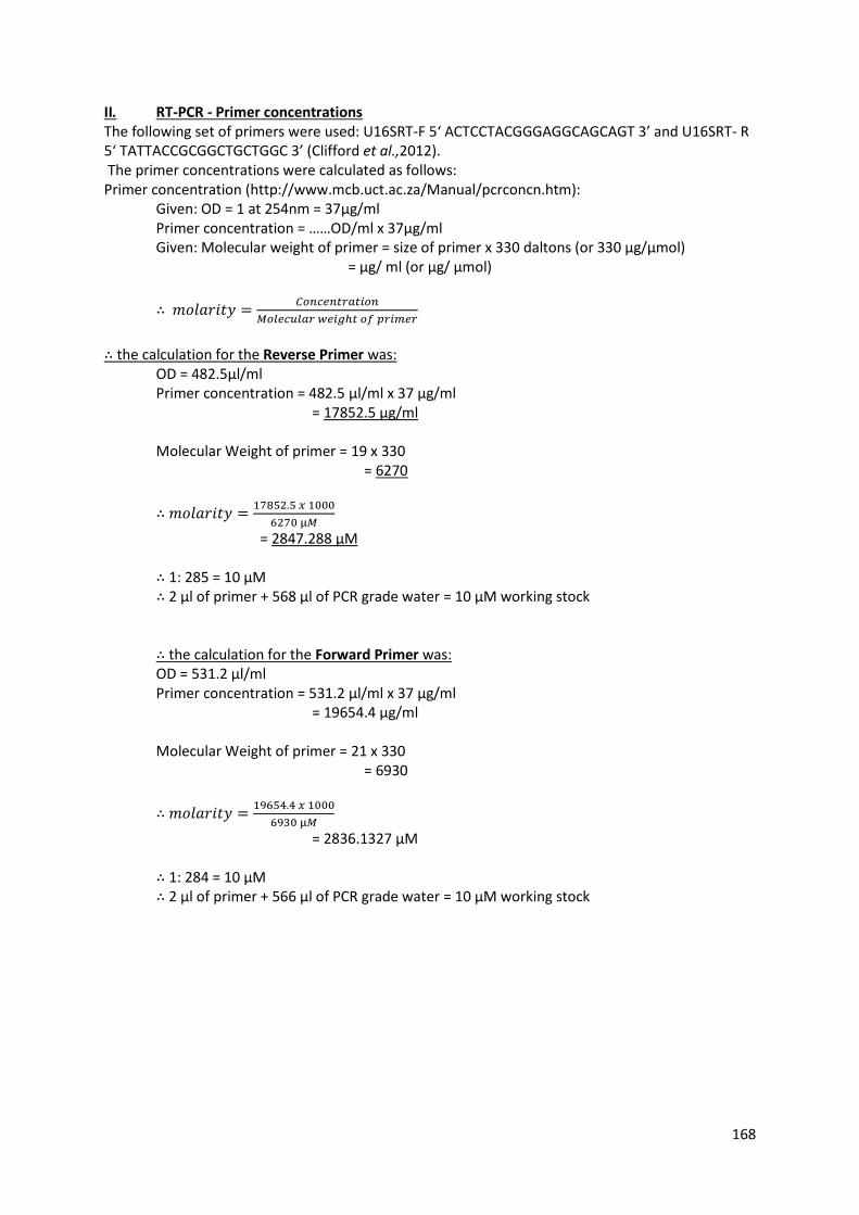
168

II. RT-PCR - Primer concentrations The following set of primers were used: U16SRT-F 5‘ ACTCCTACGGGAGGCAGCAGT 3’ and U16SRT- R 5‘ TATTACCGCGGCTGCTGGC 3’ (Clifford et al.,2012). The primer concentrations were calculated as follows: Primer concentration (http://www.mcb.uct.ac.za/Manual/pcrconcn.htm): Given: OD = 1 at 254nm = 37µg/ml Primer concentration = ……OD/ml x 37µg/ml Given: Molecular weight of primer = size of primer x 330 daltons (or 330 µg/µmol) = µg/ ml (or µg/ µmol)

∴ 𝑚𝑜𝑙𝑎𝑟𝑖𝑡𝑦 =𝐶𝑜𝑛𝑐𝑒𝑛𝑡𝑟𝑎𝑡𝑖𝑜𝑛

𝑀𝑜𝑙𝑒𝑐𝑢𝑙𝑎𝑟 𝑤𝑒𝑖𝑔ℎ𝑡 𝑜𝑓 𝑝𝑟𝑖𝑚𝑒𝑟

∴ the calculation for the Reverse Primer was: OD = 482.5µl/ml Primer concentration = 482.5 µl/ml x 37 µg/ml = 17852.5 µg/ml Molecular Weight of primer = 19 x 330 = 6270

∴ 𝑚𝑜𝑙𝑎𝑟𝑖𝑡𝑦 =17852.5 𝑥 1000

6270 µ𝑀

= 2847.288 µM ∴ 1: 285 = 10 µM

∴ 2 µl of primer + 568 µl of PCR grade water = 10 µM working stock

∴ the calculation for the Forward Primer was: OD = 531.2 µl/ml Primer concentration = 531.2 µl/ml x 37 µg/ml = 19654.4 µg/ml Molecular Weight of primer = 21 x 330 = 6930

∴ 𝑚𝑜𝑙𝑎𝑟𝑖𝑡𝑦 =19654.4 𝑥 1000

6930 µ𝑀

= 2836.1327 µM ∴ 1: 284 = 10 µM

∴ 2 µl of primer + 566 µl of PCR grade water = 10 µM working stock

169

Appendix D Preparation of Agarose gels

I. Preparation of 1% agarose gel

- Add 1 g agarose (Lonza, USA) to 100 ml 1X TAE

- Dissolve by heating agarose in the microwave for a few minutes

- Allow to cool to approximately 45°C

- Add 0.5 µg/ml of Ethidium Bromide (EtBr) (Fluka, Switzerland)

- Pour gel into mould of appropriate size

- Position appropriate comb at the top end of the mould

- Allow gel to set at room temperature

- Remove comb

- Submerge gel into electrophoresis tank containing 1X TAE buffer

170

Appendix E Molecular weight marker- Hyperladder ITM (Bioline, UK)

This type of marker is both a molecular weight marker a well as a quantitative marker. This marker

contains a mixture of DNA fragments of pre-determined sizes that can be compared with the sample

DNA, therefore the size(s) of the separated DNA fragments could be determined.

171

Appendix F 16S rRNA library preparation

I. Short 16S rRNA PCR

An end-point PCR assay targeting the 16S rRNA gene, made use of the following modified

primer pair: 5’GTGCCAGCHGCYGCGGT3’; and 806R: 5’GGACTACNNGGGTWTCTAAT3’ (modified from

Caparoso et al (2011). These primers were modified to include ambiguous bases in order to target

more species.

The PCR reaction master mix contained 12.5 µL of 2x MyTaqTM HS mix (Bioline, MA, USA), 0.75 µl of

Dimethyl sulphoxide (DMSO), 4 µl PCR grade water (Teknovea, Fisher, Hollister, CA), 2 µl each 515F

short and 806R short primers from a final stock of 10 µM (Sigma custom oligos, USA, MO 63103).

PCR reactions were performed up to a final volume of 25.25 µl per reaction.

An aliquot of 21.25 µl of master mix was added into each well, into which 4 µl of template DNA of

each of the samples were added. Four controls were included in each of the sequencing runs. The

four controls included an E. coli DNA control, one NTC, and two BEI controls (which are used for 16S

rRNA gene sequencing). One of the BEI controls was HM-783D (bei resources, VA, USA) which is

genomic DNA from microbial mock community B (staggered and low concentration). The other BEI

control was HM-782D which is genomic DNA from microbial mock community B (even and low

concentration). Both HM-783D and HM-782D contained genomic DNA from 20 bacterial strains

containing staggered or even ribosomal RNA operon counts respectively. And lastly, the E.coli DNA

control was at a final concentration of 60 ng total genomic DNA. The sequencing plate was vortexed

(to mix reagents) and briefly centrifuged (GS-6R Centrifuge, Beckam Coutler, CA, USA) up to 300 rpm

(to collect all reagents at bottom of wells).

PCR cycling conditions included an initial denaturation step for 3 min at 95°C, followed by 10 cycles

of 30 sec at 95°C, 30 sec at 50°C and 1 sec at 72°C. This was followed by 5 min at 72°C for a final

extension. The PCR reactions were performed on the MJ Research Ptc-225 Tetrad Peltier Thermal

Cycler (MJ Research Inc. Canada, QC).

172

II. Long 16S rRNA PCR

The next end-point PCR made use of the same PCR primers as above (Caparoso et al (2011)

with added barcodes unique to each sample. The PCR reaction Master mix contained 12.5µL of 2x

MyTaqTM HS mix (Bioline, MA, USA), 0.75 µl of Dimethyl sulphoxide (DMSO), 4 µl PCR grade water

(Teknovea, Fisher, Hollister, CA) and 4 µl of the 515F short and 806R short primer mix (which

contained both forward and reverse primers from a final stock of 10 µM) (Sigma custom oligos, USA,

MO 63103). PCR reactions were performed in a final volume of 25.25 µl per reaction.

An aliquot of 21.25 µl of master mix was combined with 4 µl of each sample (taken from the short

PCR reaction) in a 96 well sequencing plate. Similarly, the four controls from the short PCR was

added to reaction master mix. After sealing the plate, it was vortexed and briefly centrifuged (GS-6R

Centrifuge, Beckam Coutler, CA, USA) up to 300 rpm.

PCR cycling conditions included an initial denaturation step for 3 min at 95°C, followed by 30 cycles

of 30 sec at 95°C, 30 sec at 50°C and 1 sec at 72°C. This was followed by 5 min at 72°C for final

extension. The PCR reactions were performed on the MJ Research Ptc-225 Tetrad Peltier Thermal

Cycler (MJ Research Inc. Canada, QC).

III. PCR product clean-up

This PCR product cleanup step was modified from the Agencourt® Ampure® XP PCR

Purification Protocol (Beckman Coulter, USA, CA) for removal of 300 bp and below, as the

approximate expected size of the amplicons are between 400 -500bp. The Agencourt beads were

gently shaken to resuspend magnetic particles that may have settled. The beads (0.65 µl per

reaction) were aliquoted into each well of the long PCR plate and was mixed ten times using a

pipette. The beads and the samples were incubated at room temperate for five minutes before the

plate was sealed, vortexed and spun in the centrifuge (GS-6R Centrifuge, Beckam Coutler, CA, USA)

at 300 rpm.

The reaction plate was placed onto the Agencourt SPRIPlate 96 Super Magnet Plate and allowed to

rest for two minutes, therefore to separate the beads from the solution. The clear solution was

aspirated from the reaction mixture plate and discarded. 70% EtOH (200 µl) was dispensed into each

well of the reaction plate and left to incubate for 30 seconds at room temperature. The ethanol was

173

aspirated and discarded. This wash step was repeated two more times. Finally, the reaction plate

was left for a minimum of one minute, allowing for any remaining ethanol to evaporate. The

reaction plate was removed from the magnetic plate, and 40 µl of TE elution buffer (TRIS-EDTA

buffer, pH 8.0, Grade: Biotechnology grade, Quality Biological Inc., USA, OH) was added to each well

of the reaction plate. The plate was sealed, vortexed and quickly spun in the centrifuge (GS-6R

Centrifuge, Beckam Coutler, CA, USA) at 300 rpm. The reaction plate was incubated for 1 minute on

the magnetic plate, to eparate the beads from the solution. And finally, 35 µl of the eluent was

transferred (without any beads) to a new plate (Clear 96 well Semi skirted plate, 10/unit, Flat top,

Phenix Research Products, USA, NC).

IV. Agarose Gel electrophoresis

A 1x loading dye (2 µl) was added to 5 µl of PCR amplicon (obtained from the long PCR clean

up) and 6.8 µl of this template dye mix (InvitrogenTM; Life Technologies, USA, CA) was loaded onto a

1.5% agarose gel (Agarose genetic Analysis Grade 100 g, Fisher ScientificTM, USA, NJ,) containing EtBr

(1 µl/100 ml) (UltraPureTM mg/ml Ethidium Bromide; Life Technologies, USA, CA), (1 µl/100 ml).

TrackIt 1kb Plus DNA ladder (InvitrogenTM; Life Technologies, USA, CA) was included in the gel as a

Molecular weight marker. The amplicon DNA was electrophoresed for 90 minutes at 80 volts (Power

PAC 300, Bio-Rad Laboratories Inc, USA, CA). The gels were viewed using a variable mode imager

with its software (Typhoon 9410 Molecular Imager and Typhoon Scanner Control, GE Amersham

Molecular Dynamics, USA, PA).

V. Quantification of samples using Quant-IT

In order for the fluorophore to be diluted from 200X to 1X, 278 µl of BR reagent fluorophore

was added to 55 322 µl of buffer (DNA quantitation kit, Quant-iTTM Broad-Range DNA assay kit,

InvitrogenTM (Molecular Probes®), USA, CA). An aliquot of 5 µl of amplicon DNA (from the purified

long PCR) was added to 100 µl of a 1X fluorophore mix in a 96 well plate. Similarly, each of the

controls were added (5 µl) in triplicate to 100 µl of a 1X fluorophore mix. The 96 well plate was

placed on a microplate reader (Infinte® M1000 Pro, Tecan, GmbH and I-ControlTM, Tecan, Version

1.7, GmbH software) to calculate DNA concentrations of each sample and controls.

174

VI. Pooling of PCR products, pool clean-up and quantification of pools

Equimolar amounts of each amplicon was determined using a custom R script developed by

collaborators at J Craig Venter Institute (JCVI) (Maryland, USA). Two sample pools were created by

combining equimolar amounts of 96 samples per pool. Combining equimolar amounts of amplicon

DNA ensures that an appropriate number of sequences per sample would be obtained.

Quantification of pools was done with the use of the Nanodrop spectrophotometer (Nanadrop ND

1000 Spectrophotometer, Thermo Scientifc, ND 1000, USA, DE), using its own software (ND 1000,

Thermo Scientific, Version 3.7.1, USA, DE). The two pools were combined and the new concentration

measured on the Nanodrop spectrophotometer.

The Agencourt AMPure beads (Agencourt AMPure XP, Beckman Coulter, USA, CA) were added to the

final pool aliquot in a 1:1 ratio. The beads and the pooled aliquots were mixed and allowed to

incubate at room temperature for five minutes in order to obtain maximum binding (recovery).

Tubes were used instead of plates, and the protocol was continued as previously described in 2.5.3.

However 60 µl of TE elution buffer was used instead of 40 µl. Thereafter, 60 µl of the eluent was

transferred to new tubes (without transferring any beads).

The DNA concentration of the combined eluents were determined with the use of the Nanadrop

spectrophotometer, and the final volume was calculated.

VII. Separate primer dimers from pooled DNA

Primer dimers were removed from the pooled DNA by running a 1.5% agarose gel for size

selection. A 1x loading dye (5 µl) was added to 6.6 µl of the pooled DNA and loaded onto a 1.5%

agarose gel (Agarose genetic Analysis Grade 100 g, Fisher ScientificTM, USA, NJ,) containing EtBr

(UltraPureTM mg/ml Ethidium Bromide; Life Technologies, USA, CA). TrackIt 1kb Plus DNA ladder

(InvitrogenTM; Life Technologies, USA, CA) was included in the gel as a Molecular weight marker. DNA

samples were electrophoresed for 30 minutes at 35 volts, followed by 45 minutes at 40 volts and

lastly for 3 hours at 70 volts (Power PAC 300, Bio-Rad Laboratories Inc, USA, CA). The gels were

viewed using a variable mode imager with its software (Typhoon 9410 Molecular Imager and

Typhoon Scanner Control, GE Amersham Molecular Dynamics, USA, PA). The gel was viewed under a

UV lamp (EL series 8-Watt Ultraviolet Lamps, UVP®INC, USA, CA) and trans-illuminator (Dark Reader

DR89X Trans illuminator, Clare Chemical Research, Inc., USA, CO). DNA bands ranging between 400

175

to 500 bp, corresponding to the expected amplicon length, were excised from the agarose gel with a

sterile blade, and placed into a sterile 1.5 ml Eppendorf tube, ensuring that the gel pieces do not

exceed 300 mg per tube.

VIII. Gel Product clean up and DNA quantification

The DNA was extracted from the gel slices using the QIAquick Gel extraction kit (Qiagen,

USA,MA) (full protocol below). The following modifications to the extraction protocol included an

optional washing step after binding the DNA to the column (step 9 in full protocol below). A second

modification entailed incubating the spin column, containing Buffer PE, at 37 ˚C for 5 minutes,

before centrifuging for one minute (step 10 in full protocol). This additional step was repeated. The

final modification was introduced at step 13, where the spin column was incubated for 1 minute

with 50 µl elution buffer prior to centrifugation. The eluted DNA was quantified on a

spectrophotometer to obtain the final DNA concentration. These gel purified products were

considered ready for sequencing.

QIAquick Gel Extraction Kit Protocol (Qiagen Silicon Valley, Redwood city, CA, USA) 1. Excise DNA fragment from agarose gel with a clean, sharp scalpel. 2. Weigh the gel slice in a colorless tube. Add 3 volumes of Buffer QX1 to 1 volume gel (100 mg ~ 100 ml). The maximum amount of gel slice per QIAquick column is 400 mg; for gel slices >400 mg, use more than one column. 3. Incubate at 50°C for 10 min (or until the gel slice has completely dissolved). To help dissolve gel, mix by vortexing the tube every 2-3 min during the incubation. 4. After the gel slice has dissolved completely, check that the color of the mixture is yellow. 5. Add 1 gel volume of isopropanol to the sample and mix. 6. Place a QIAquick spin column in a provided 2-ml collection tube. 7. To bind DNA, apply the sample to the QIAquick column, and centrifuge for 1 min. 8. Discard flow-through and place the QIAquick column back in the same collection tube. 9. (Optional): Add 0.5 ml of Buffer QX1 to QIAquick column and centrifuge for 1 min. 10. To wash, add 0.75 ml of Buffer PE to QIAquick column and centrifuge for 1 min. 11. Discard flow-through and centrifuge the QIAquick column for an additional 1 min at ~13,000 rpm. 12. Place QIAquick column into a clean 1.5-ml microfuge tube. 13. To elute DNA, add 50 ml of 10 mM Tris-HCl, pH 8.5 of H2O to the center of the QIAquick column and centrifuge for 1 min at maximum speed. Alternatively, for increased DNA concentration, add 30 ml elution buffer to the center of the QIAquick column, let stand for 1 min, and then centrifuge for 1 min.

IX. Quantification of the final pool

In order to maximise the amount of sequencing information, and therefore reducing the cost

per base sequenced, it is important to optimise the amount of DNA library that is prepared for a

176

sequencing run (Buehler et al., 2010). qPCR is used to accurately determine the library quantity at a

high sensitivity of detection (Buehler et al., 2010). qPCR of final DNA pools also minimises over-

estimation of the DNA concentration by only measuring fragments with adapters ligated to both

ends as only these will be amplified and sequenced in subsequent steps.

Library DNA was quantified using the Kapa Illumina library quantification kit (Kapa biosystems, USA,

MA). This kits included KAPA SYBR® Fast ABI Prism qPCR kit, 1 ml of 10X GA primer premix (Primer

P1: 5’-AAT GAT ACG GCG ACC ACC GA-3’, and Primer P2: 5’-CAA GCA GAA GAC GGC ATA CGA-3’).

Quantification of the DNA was performed with slight modifications. Modifications included ten-fold

dilutions of the library DNA starting at 1:120 dilution, followed by 1:1200 and 1:12000 dilutions.

(A 1:120 dilution was made by adding 238 µl of TE+0.05% Tween 20 buffer (was prepared by

adding 500 µl of 1 M Tris-HCl, pH 8.0 buffer solution (Life Technologies) to 49.5 mL of molecular

grade biology water (Quality Biological). Each DNA dilution was evaluated in triplicate using qPCR.

49.25 mL of 1X TE buffer was measured out and was added to 25 µl of Tween 20 (Sigma Aldrich), this

was thoroughly mixed and stored at room temperature) to 2 µl of the library DNA. The next dilution

was a 1:1200 which was made by adding 45 µl of TE+0.05% Tween 20 buffer to 5 µl of the 1:120

dilution library. And finally, the last dilution was a 1:12000 which was made by adding 45 µl of TE +

0.05% Tween 20 buffer to 5 µl of the 1:200 dilution library).

Similarly, the PCR standards were set up in triplicate. The final qPCR reaction volume of 10 µl

included 6 µl of master mix and 4 µl sample (diluted library DNA). qPCR controls included 4 µl of

water (for NTC), or 4 µl DNA for standards, or 4 µl Shrimp Aqu BIOFLOC 3-PE-IL55-01 (for PC).

The PCR reactions were performed on the ABI Prism 7900HT Sequence detection system using the

SDS Enterprise Database (Applied Biosystems). PCR cycling conditions were performed according to

the KAPA library quantification kit instructions. The PCR cycling conditions included an initial

denaturation step for 5 min at 95°C, followed by 35 cycles of 30 sec at 95°C and 45 sec at 50°C.

After all the samples were quantified, and the failed samples were omitted, the slope of the linear

regression line and R2 values were calculated. The slope was meant to be between -3.58 and -3.10

with a R2 value of 0.99.

177

X. Integrity and size of DNA products for each of the dilutions

The DNA product for each of the dilutions were electrophoresed on a 0.8% agarose gel (E-

gel® pre-cast agarose gels (InvitrogenTM, CA, USA) to confirm the size of the amplicons. A final

volume of 20 µl (3 µl of the respective dilution, 16 µ of water and 1 µl pf 6X TrackItTM Cyan/Yellow

loading buffer (InvitrogenTM, CA,USA) was loaded onto the agarose gel. The NTC and TrackitTM 1kb

Plus DNA ladder (InvitrogenTM, CA,USA) were included on the gel. The E-gels (E-Gel® General purpose

gels, 0.8%, Life Technologies) were electrophoresed for 30 minutes, and once completed the PCR

products were viewed using the Bio-Rad Gel DocTM System (Bio-Rad, CA,USA) .

Sequencing steps

XI. Library denaturation and sequencing

Paired end libraries were prepared with the MiSeq Reagent Kit v3, 600 Cycles (Illumina,

CA,USA). The target read length for the libraries were 250 bp. DNA was diluted to a final

concentration of 20 pM in 10 mM Tris-Hcl, pH8.5 (Life Technologies, CA,USA). The denatured DNA

was diluted to a final concentration of 4 pM in hybridisation buffer (HT1) (supplied by the

manufacturer). The denatured pHIx control was diluted to a final concentration of 4 pM in HT1

buffer. This denatured PhiX control was added at 5% by adding 50 µl of 4pM denatured sample DNA

to 950 µl of 4 pM denatured PhiX control. A total volume of 600 µl of the denatured DNA library was

loaded onto the Illumina MiSeqTM platform for sequencing. Base calling and demultiplexing of

samples was performed using CASAVA version 1.8.2 software (Illumina, CA, USA) (which is part of

the Illumina suite of tools). This resulted in separate FASTQ files for each sample labelled with the

sample name.

178

Appendix G Running of the 16S rRNA YAP pipeline

Yap took on a systematic approach, whereby the initial step of the workflow was to assess the read

quality statistics, and these files were embedded in the FASTQ files. These quality assessments were

performed using the FASTX toolkit ((http://hannonlab.cshl.edu/fastx_toolkit/), whereby the quality

was assessed using Phred quality scores (Q scores) (Illumina Proprietary. Quality Scores for Next-

Generation Sequencing, 2011) (Figure 4.5, step 1). The quality of each of these reads are most

typically described with a number for each base. A good quality read on average is estimated at

around 40 across all the bases (if not more). In the case of MiSeq, the overall quality is slightly lower,

therefore the threshold was set at 35. However, the lesser the quality, the more sequencing errors

will occur, and the more uncertainty there would be further downstream.

Most often than not, quality reads are known to deteriorate near the ends of the reads, therefore

following quality assessment, each of the 300 base-pair long paired-end reads were first trimmed

using a low threshold of Q=3. This was performed with the use of SolexaQA’s Dynamic Trim function

(Cox et al., 2010) (Figure 4.5, step 1). In YAP, trimming occurs at two points: 1) at the beginning of

processing, where a low quality threshold is adopted to ~3 phred score. This is to keep as many

reads as possible); 2) thereafter, the two mate pairs have been overlapped and stitched together

with FLASH (this is the final trim and the threshold for trimming is higher: ~ 25 phred score).

After the initial trimming, FLASH’s algorithim was used whereby the trimmed paired end reads were

overlapped (Magoč & Salzberg 2011) (Figure 4.5, step 1). A final trim at a higher quality threshold of

Q=25 was performed once again with the use of SolexaQA’s Dynamic trim function (Figure4. 5, step

2). In order to reduce the data size, the duplicate reads were recorded and then removed (Figure

4.5, step 3).

The next step of the workflow was to verify that all reads which were either not corresponding to

the 16S rRNA gene or was shorter than 220 bases were removed, and that these reads were in the

correct orientation of 5’ to 3’ direction. This was achieved by comparing these reads to the SILVA

database (Pruesse et al., 2007; Quast et al., 2013) using an algorithm called Nearest Alignment Space

Termination (NAST) (DeSantis et al., 2006(a)) for creating multiple sequence alignments (MSA) with

sequences in the SILVA 16 S database (Pruesse et al., 2007; Quast et al., 2013) (Figure 4.5, step 4).

179

The next stage of the workflow entailed removing chimeric reads (which are made up of more than

one organism) by comparing each of the reads to the SILVA database of pure organisms and

chimeras. This was done with the use of a chimera detection program known as UCHIME (Edgar et

al., 2011) which was integrated into the mothur software (Schloss et al., 2009).

An additional quality check step was performed, whereby the reads were aligned to the 16S rRNA

gene reference region of Escherichia coli (obtained from NCBI). This alignment was trimmed to

remove ends with less than 90% of the maximum coverage, as well as was used to remove reads

that did not align to the targeted V4 region (Figure 4.5, step 5).

Furthermore, a clustering algorithm implemented in the software the CD-HIT-EST within the CD-HIT

suite was used to cluster all the good quality reads into OTUs (Huang, Niu, Gao, Fu, & Li, 2010).The

YAP workflow performs clustering at four different similarity levels, 90%, 95%, 97% and 99%.

Recorded duplicate reads were added to the appropriate OTU cluster before calculating the final

OTU cluster size (Figure 4.5, step 6).

Within mothur, taxonomic information was assigned to OTU’s with the use of naïve Bayesion

classifier (Cole et al., 2009). The taxonomic labels were derived from a normalised Ribosomal

database project (RDP) training dataset. For computational efficiency, only the exemplar sequence

representing each of the OTU clusters could be taxonomically classified. The exemplar sequence is

equidistant from every sequence in the cluster of the “centroid” (A cluster that is defined by one

sequence). Following taxonomic classification, by adding together the cluster size of OTU clusters

labelled with the taxonomic label of interest, YAP had then computed the aggregate sequence

counts for any given taxonomic level (Figure 4.5, step 6).

180

Appendix H

Season (Rate ratio)

Taxa Phylum P-value Spring Summer Autumn Winter

Acidobacteria Acidobacteria 1.31E-07 2.01 2.42 1.58 1

Acidomicrobiales Acidobacteria 1.82E-04 1.55 1.43 1.13 1

Skermanella Actinobacteria 2.55E-09 2.09 3.09 2.04 1

Unclassfied Actinobacteria 3.79E-03 1.66 1.74 1.4 1

Unclassfied Actinobacteria 3.79E-03 1.66 1.74 1.4 1

Unclassified Actinobacteria 3.30E-02 0.903 1.128 1.067 1

Unclassified Actinobacteria 3.30E-02 0.903 1.128 1.067 1

Unclassifed Actinobacteria 4.94E-02 1.3 1.41 1.5 1

Unclassified Actinobacteria 1.77E-02 1.12 1.5 1.37 1

Micromonosporaceae Actinobacteria 6.07E-03 1.02 1.39 1.29 1

Blastococcus Actinobacteria 2.50E-05 1.33 1.72 1.41 1

Geodermatophilaceae Actinobacteria 6.22E-05 1.19 1.54 1.32 1

Solirubrobacteraceae Actinobacteria 2.02E-04 1.19 1.64 1.34 1

Solirubrobacter Actinobacteria 2.02E-04 1.19 1.64 1.34 1

Adaeribacter Actinobacteria 2.62E-02 1.09 1.55 1.49 1

Pseudonocardia Actinobacteria 3.37E-03 1.08 1.37 1.12 1

Solirubrobacterales Actinobacteria 1.74E-03 1.05 1.39 1.21 1

Unclassified Actinobacteria 4.53E-04 1.05 1.44 1.27 1

Pseudomonocardiaceae Actinobacteria 3.25E-03 1.04 1.35 1.2 1

Unclassified Actinobacteria 4.62E-02 0.978 0.846 0.793 1

Microbacteriaceae Actinobacteria 7.26E-03 0.834 0.68 0.719 1

Unclassfied Actinobacteria 3.10E-02 0.818 0.663 0.673 1

Micrococcaceae Actinobacteria 1.62E-02 0.761 0.713 0.823 1

Kocuria Actinobacteria 9.13E-03 0.666 0.574 0.674 1

Micrococcus Actinobacteria 7.89E-03 0.586 0.52 0.714 1

Flavobacteriaceae Bacteroidetes 2.17E-04 0.651 0.334 0.502 1

Flavobacteria Bacteroidetes 1.84E-04 0.634 0.317 0.492 1

Flavobacteriales Bacteroidetes 1.84E-04 0.634 0.317 0.492 1

Hymenobacter Bacteroidetes 4.88E-04 0.818 0.426 0.546 1

Sphingobacteriaceae Bacteroidetes 1.97E-02 0.62 1.541 0.652 1

Bacteroidia Bacteroidetes 3.57E-04 0.391 1.251 1.756 1

Bacteroidales Bacteroidetes 3.57E-04 0.391 1.251 1.756 1

Porphyromonadaceae Bacteroidetes 9.41E-04 0.36 1.05 1.44 1

Chlorflexi Chlorflexi 9.41E-04 0.36 1.05 1.44 1

Chloroplast Cyanobacteria_Chloroplast 7.73E-04 1.64 1.74 1.33 1

Chloroplast_order_ incertaw_sedis

Cyanobacteria_Chloroplast 4.50E-07 1.226 0.535 0.591 1

Chloroplast Cyanobacteria_Chloroplast 4.50E-07 1.226 0.535 0.591 1

Streptophyta Cyanobacteria_Chloroplast 4.50E-07 1.226 0.535 0.591 1

Table I: 103 taxa affected by season, including p-values and rate ratios according to GLMM analysis

181

Cyanobacteria Cyanobacteria_Chloroplast 1.61E-03 1.133 0.432 0.626 1

Cyanobacteria_order_ incertae_sedis

Cyanobacteria_Chloroplast 4.35E-11 2.06 1.18 0.98 1

Cyanobacteria_chloroplast Cyanobacteria_Chloroplast 4.35E-11 2.06 1.18 0.98 1

Acetobacteraceae Firmicutes 5.08E-10 1.466 0.75 0.698 1

Bacillaceae Firmicutes 2.59E-06 1.6 1.96 1.45 1

Paenibacillaceae Firmicutes 3.30E-02 0.907 1.162 1.094 1

Carnobacteriaceae Firmicutes 2.46E-02 1.03 1.24 1.47 1

Lachnospiraceae Firmicutes 4.76E-02 0.76 0.605 0.756 1

Ruminococcaceae Firmicutes 5.01E-04 0.33 0.452 0.825 1

Bacilli Firmicutes 3.57E-04 0.327 0.598 0.971 1

Clostridiales Firmicutes 3.30E-02 0.78 0.785 0.885 1

Clostridia Firmicutes 2.56E-03 0.451 0.532 0.839 1

Firmicutes Firmicutes 2.46E-03 0.451 0.534 0.84 1

Staphylococcaceae Firmicutes 1.66E-03 0.659 0.681 0.85 1

Lactobacillales Firmicutes 4.77E-04 0.58 0.396 0.625 1

Gemmatimonadetes Gemmatimonadetes 3.21E-03 0.579 0.468 0.639 1

Gemmatimonadetes Gemmatimonadetes 4.70E-02 1.37 1.28 1.31 1

Gemmatimonadales Gemmatimonadetes 4.70E-02 1.37 1.28 1.31 1

Gemmatimonadaceae Gemmatimonadetes 4.70E-02 1.37 1.28 1.31 1

Gemmatimonas Gemmatimonadetes 4.70E-02 1.37 1.28 1.31 1

Singulispaera Planctomycetes 4.70E-02 1.37 1.28 1.31 1

Planctomycetacia Planctomycetes 2.56E-03 1.93 2.14 1.75 1

Planctomycetales Planctomycetes 1.66E-03 1.88 1.8 1.54 1

Planctomycetaceae Planctomycetes 1.66E-03 1.88 1.8 1.54 1

Planctomycetes Planctomycetes 1.66E-03 1.88 1.8 1.54 1

Unclassified Proteobacteria 1.90E-03 1.87 1.8 1.53 1

Unclassified Proteobacteria 4.73E-06 2.16 2.36 1.81 1

Unclassified Proteobacteria 4.73E-06 2.16 2.36 1.81 1

Unclassified Proteobacteria 4.73E-06 2.16 2.36 1.81 1

Unclassified Proteobacteria 4.73E-06 2.16 2.36 1.81 1

Rhodospirillales Proteobacteria 2.44E-06 1.89 2.43 1.66 1

Methylobacteriaceae Proteobacteria 1.25E-08 1.73 2.25 1.59 1

Roseomonas Proteobacteria 5.34E-03 1.37 1.7 1.34 1

Amaricoccus Proteobacteria 8.75E-04 1.36 1.53 1.24 1

Unclassified Proteobacteria 1.69E-02 1.31 1.46 1.22 1

Rhizobales Proteobacteria 1.08E-05 1.53 1.31 1.24 1

Rubellimicrobium Proteobacteria 4.29E-03 1.41 1.24 1.1 1

Rhodobacterales Proteobacteria 3.25E-03 1.33 1.17 1.01 1

Rhodobacteraceae Proteobacteria 2.48E-05 1.28 1.09 1.07 1

Proteobacteria Proteobacteria 2.48E-05 1.28 1.09 1.07 1

Unclassified Proteobacteria 1.29E-04 1.15 1.07 1.03 1

Sphingomondales Proteobacteria 4.06E-02 2.13 1.92 1.55 1

Sphingomondaceae Proteobacteria 2.56E-03 1.179 0.91 0.946 1

Rhodospirillaceae Proteobacteria 1.80E-02 1.176 0.939 0.956 1

Table I continued…..

182

Alphaproteobacteria Proteobacteria 6.09E-11 2.06 3.14 2.06 1

Alphaproteobacteria Proteobacteria 7.21E-05 1.47 1.47 1.25 1

Alphaproteobacteria Proteobacteria 1.07E-04 1.74 2.25 1.82 1

Unclassified Proteobacteria 1.07E-04 1.74 2.25 1.82 1

Paracoccus Proteobacteria 4.06E-02 2.13 1.92 1.55 1

Gamma Proteobacteria Proteobacteria 1.39E-02 0.975 0.785 0.932 1

Xanthomondales Proteobacteria 1.43E-06 0.654 0.371 0.645 1

Xanthomondaceae Proteobacteria 1.20E-05 0.734 0.435 0.604 1

Moraxellaceae Proteobacteria 9.64E-06 0.729 0.421 0.603 1

Pseudomonadales Proteobacteria 6.32E-06 0.577 0.196 0.652 1

Enterobacteriales Proteobacteria 3.84E-06 0.562 0.21 0.623 1

Enterobacteriaceae Proteobacteria 3.36E-03 0.504 0.371 0.578 1

Unclassified Unclassified 3.36E-03 0.504 0.371 0.578 1

Unclassified Unclassified 2.56E-03 1.45 1.57 1.32 1

Unclassified Unclassified 2.56E-03 1.45 1.57 1.32 1

Unclassified Unclassified 2.56E-03 1.45 1.57 1.32 1

Unclassified Unclassified 2.56E-03 1.45 1.57 1.32 1

Unclassified Unclassified 2.56E-03 1.45 1.57 1.32 1

Unclassfied Unclassified 1.69E-02 0.805 0.597 0.782 1

Unclassfied Unclassified 1.69E-02 0.805 0.597 0.782 1

Verrucomicrobia Verrucomicrobia 1.69E-02 0.805 0.597 0.782 1

Table I continued…..

183

House type (Rate Ratio)

Taxa Phylum Pvalue Flat Shack Other House

Kocuria Actinobacteria 2.48E-05 1.108 1.435 0.717 1

Lactobacillales Firmicutes 1.76E-04 1.156 1.576 0.881 1

Enterobacteriales Proteobacteria 1.84E-04 0.726 1.489 0.575 1

Enterobaceriaceae Proteobacteria 1.84E-04 0.726 1.489 0.575 1

Corynebacterium Actinobacteria 1.98E-04 0.71 1.61 1.02 1

Bacilli Firmicutes 2.02E-04 1.112 1.283 0.883 1

Unclassified Unclassified 2.02E-04 0.932 0.767 1.249 1

Unclassified Unclassified 2.02E-04 0.932 0.767 1.249 1

Unclassfied Unclassified 2.02E-04 0.932 0.767 1.249 1

Unclassified Unclassified 2.02E-04 0.932 0.767 1.249 1

Unclassified Unclassified 2.02E-04 0.932 0.767 1.249 1

Corynebacteriaceae Actinobacteria 2.05E-04 0.692 1.599 1.017 1

Carnobacteriaceae Firmicutes 1.35E-03 1.45 1.714 0.925 1

Micrococcaceae Actinobacteria 2.12E-03 1.1 1.28 0.93 1

Paracoccus Proteobacteria 2.12E-03 1.229 1.209 0.706 1

Cyanobacteria Cyanobacteria_chloroplast 2.12E-03 0.509 0.658 1.118 1

Cyanobacteria_order_ incertae_sedis

Cyanobacteria_chloroplast 2.12E-03 0.509 0.658 1.118 1

Staphylococcaceae Firmicutes 2.12E-03 1.049 1.612 0.846 1

Planctomycetes Planctomycetes 2.13E-03 1.248 0.831 1.406 1

Planctomyceracia Planctomycetes 2.27E-03 1.242 0.833 1.402 1

Planctomycetales Planctomycetes 2.27E-03 1.242 0.833 1.402 1

Planctomycetaceae Planctomycetes 2.27E-03 1.242 0.833 1.402 1

Myxococcales Proteobacteria 2.56E-03 1.004 0.796 1.127 1

Pseudomonadales Proteobacteria 3.31E-03 1.206 1.558 0.689 1

Moraxellaceae Proteobacteria 3.37E-03 1.343 1.683 0.715 1

Unclassfied Actinobacteria 5.24E-03 0.92 0.818 1.288 1

Unclassified Actinobacteria 5.24E-03 0.92 0.818 1.288 1

Unclassfied Actinobacteria 5.24E-03 0.92 0.818 1.288 1

Unclassfied Chlorflexi 5.88E-03 1.4 1.19 1.36 1

Unclassfied Chlorflexi 5.88E-03 1.4 1.19 1.36 1

Unclassified Chlorflexi 5.88E-03 1.4 1.19 1.36 1

Bacillales Firmicutes 6.61E-03 1.087 1.187 0.885 1

Gammaproteobacteria Proteobacteria 7.31E-03 1.085 1.314 0.818 1

Blastococcus Actinobacteria 7.50E-03 1.055 0.857 1.185 1

Micrococcus Actinobacteria 8.57E-03 1.088 1.42 0.911 1

Thermomicrobia Chlorflexi 1.08E-02 1.34 1.16 1.29 1

Firmicutes Firmicutes 1.50E-02 1.09 1.21 0.85 1

Chlorflexi Chlorflexi 1.52E-02 1.24 1.04 1.33 1

Gemmatimonadetes Gemmatimonadetes 1.62E-02 1.003 0.836 1.166 1

Gemmatimonadetes Gemmatimonadetes 1.62E-02 1.003 0.836 1.166 1

Table II: 63 most abundant taxa affected by house type, including p-values and rate ratios according to GLMM

analysis.

184

Pets (Rate ratio)

Taxa Phyla P-value No Yes

Unclassified Firmicutes 0.00611 1 1.25

Unclassified Firmicutes 0.00611 1 1.25

Bacillaceae Firmicutes 0.01491 1 1.31

Bacillales Firmicutes 0.01617 1 1.16

Gemmatimonadales Gemmatimonadetes 1.62E-02 1.003 1.836 1.166 1

Gemmatimonadaceae Gemmatimonadetes 1.62E-02 1.003 0.836 1.166 1

Gemmatimonas Gemmatimonadetes 1.62E-02 1.003 0.836 1.166 1

Alphaproteobacteria Proteobacteria 1.62E-02 1.006 0.758 0.933 1

Alphaproteobacteria Proteobacteria 1.62E-02 1.006 0.758 0.933 1

Cyanobacteria_chloroplast Cyanobacteria_chloroplast 1.62E-02 0.662 0.695 0.957 1

Chloroplast Cyanobacteria_chloroplast 1.62E-02 0.748 0.729 0.761 1

Chloroplast_order_ incertae_sedis

Cyanobacteria_chloroplast 1.62E-02 0.748 0.729 0.761 1

Chloroplast Cyanobacteria_chloroplast 1.62E-02 0.748 0.729 0.761 1

Acidimicrobiales Actinobacteria 1.68E-02 0.943 0.818 1.044 1

Sphingomondales Verrucomicrobia 1.91E-02 0.852 0.783 1.062 1

Singulisphaera Planctomycetes 2.91E-02 1.213 0.878 1.303 1

Arthrobacter Actinobacteria 2.91E-02 1.085 1.303 0.921 1

Unclassified Proteobacteria 3.34E-02 0.955 0.758 1.066 1

Intrasporangiaceae Actinobacteria 3.36E-02 1.31 1.16 1.02 1

Unclassfied Actinobacteria 3.37E-02 0.826 0.928 1.227 1

Verrucomicrobia Actinobacteria 3.74E-02 1.121 0.825 1.034 1

Acidobacteria Acidobacteria 4.06E-02 0.901 0.812 1.135 1

Skermanella Proteobacteria 4.23E-02 0.906 0.734 0.912 1

Flavobacteriaceae Bacteroidetes 4.26E-02 1.56 1.42 1.21 1

Unclassified Actinobacteria 4.55E-02 1.036 0.866 1.081 1

Unclassfied Actinobacteria 4.55E-02 1.036 1.866 1.081 1

Unclassified Actinobacteria 4.77E-02 1.34 1.15 1.04 1

Table III: 4 Taxa ordered according to their rate ratios obtained from GLMM analysis that are influenced by pets.

Table II continued…

185

'..... . . ·�·.. .

Appendix I Ethics Approval

·,.- . . ..::•':.'

UNIVERSITY OF CAPE TOWN

Faculty of Health Sciences

Human Research Ethics Committee

Room E52-24 Old Main Building

Groote Schuur Hospital Observatory 7925

Telephone [021] 406 6338 • Facsimile [021] 406 6411 Email: shuretta.thomas@uct.ac.za

Website: www.health.uct.ac.za/research/humanethics/forms

09 December 2013

HREC REF: 743/2013

Prof M Nicol Medical Microbiology Room 5.28, level 5 Falmouth Building

Dear Prof Nicol

PROJECT TITLE: THE ASSOCIATION BETWEEN THE BACTERIAL COMMUNITY OF INDOOR HOUSE DUST

AND RECURRENT WHEEZING IN YOUNG SOUTH AFRICAN CHILDREN (Linked to 401/2009)

Thank you for submitting your study to the Faculty of Health Sciences Human Research Ethics Committee for review.

It is a pleasure to inform you that the HREC has formally approved the above-mentioned study. We acknowledge that the student Ms Menna Duyver is also involved on this project.

Approval is granted for one year until the 30th December 2014

• Please change the supervisor to be the PI. • The student will be recognised on all communications.

Please submit a progress form, using the standardised Annual Report Form if the study continues beyond the approval period. Please submit a Standard Closure form if the study is completed within the approval period. (Forms can be found on our website: www.health.uct.ac.za/research/humanethics/forms)

Please note that the ongoing ethical conduct of the study remains the responsibility of the principal investigator.

Please quote the HREC reference no in all your correspondence.

Yours sincerely

PROFESSOR M BLOCKMAN CHAIRPERSON. FHS HUMAN ETHICS

Federal Wide Assurance Number: FWA00001637. Institutional Review Board (IRB) number: IRB00001938 This serves to confirm that the University of Cape Town Human Research Ethics Committee complies to the Ethics Standards for Clinical Research with a new drug in patients, based on the Medical Research Council (MRC-SA), Food and Drug Administration (FDA-USA), International Convention on Harmonisation Good Clinical Practice (ICH GCP) and Declaration of Helsinki guidelines.

HREC Ref 743/2013