Embed Size (px)
Citation preview
The HOL Light manual (1.1)
John Harrison
University of Cambridge Computer LaboratoryNew Museums SitePembroke Street
Cambridge CB2 3QGENGLAND
http://www.cl.cam.ac.uk/users/jrh
21 April 2000
Legal notice
HOL Light version 1.0, hereinafter referred to as “the software”, is acomputer theorem proving system written by John Harrison, a researchworker at the University of Cambridge Computer Laboratory, New Mu-seums Site, Pembroke Street, Cambridge, CB2 3QG, England. The soft-ware is copyright, c©University of Cambridge 1998.
Permission to use, copy, modify, and distribute the software and itsdocumentation for any purpose and without fee is hereby granted. In thecase of further distribution of the software the present text, includingcopyright notice, licence and disclaimer of warranty, must be includedin full and unmodified form in any release. Distribution of derivativesoftware obtained by modifying the software, or incorporating it intoother software, is permitted, provided the inclusion of the software isacknowledged and that any changes made to the software are clearlydocumented.
John Harrison and the University of Cambridge disclaim all war-ranties with regard to the software, including all implied warranties ofmerchantability and fitness. In no event shall John Harrison or theUniversity of Cambridge be liable for any special, indirect, incidentalor consequential damages or any damages whatsoever, including, butnot limited to, those arising from computer failure or malfunction, workstoppage, loss of profit or loss of contracts.
i

ii

Preface
HOL Light is a relatively new version of the HOL theorem prover (Gordon andMelham 1993). The whole implementation, even the axiomatization of the logic,has been re-engineered and simplified. Compared with other versions of HOL, it isrelatively small and clean, and makes modest demands on the machine it is run on.The material that follows is not only a tutorial on the use of HOL Light and itsinteraction language, but also provides a detailed discussion of the implementation.
HOL Light proves theorems in a system of classical higher order logic basedon polymorphic simple type theory. All proof proceeds by the application of low-level primitive rules, maintaining a high degree of reliability. However, a suite ofderived rules for proving various useful theorems automatically is provided, as is afull programming language in which users can implement their own derived rules.A number of useful mathematical theories, e.g. real analysis, are already available.
To become an expert user of HOL Light, it is necessary to know somethingabout programming in CAML Light, which is the implementation and interactionlanguage. However, for readers primarily interested in theorem proving, it’s nodoubt somewhat dispiriting to spend a long time studying functional programmingbefore even beginning to prove theorems. We have tried to minimize this problemin the organization that follows.
We begin with a short introductory chapter highlighting the basic features ofCAML and HOL, including the basic mechanism of user interaction and the princi-ples behind derived inference rules. Features of HOL and CAML are illustrated aswe go, and most readers will be able to pick up the general ideas. This introductionis followed by the two larger Parts, comprising systematic introductions to CAMLand HOL respectively. While these can be tackled in sequence, the impatient readercan read them in parallel, or even read the HOL part first and refer back to theCAML part as needed. (Indeed, there are a number of obvious parallels betweenCAML and the HOL logic, with both being an enriched version of lambda calculus,and both having a similar system of types. Reading these parts in parallel will showmany similar concepts like currying and polymorphism in two different contexts.)Since HOL Light is aimed particularly at the enthusiast who wants to implementcustom theorem-proving tools, a third Part gives an overview of the implementation,explaining the basic structure of the system and discussing various design decisions.
We hope that users interested in building custom theorem proving tools, or justin understanding the architecture of a modern theorem prover, will find somethingof interest in HOL Light and the present document. While we are writing primarilyfor those interested in theorem proving, the system might be considered interestingfor two other reasons: it is a large application of (impure) functional programming,and it includes a systematic logical development of nontrivial mathematics from itsvery foundations a la Principia Mathematica (Whitehead and Russell 1910).
I do not assume that the reader is familiar with HOL or any similar system.Some knowledge of programming and of basic logic would be of great benefit, butnot essential. However the present introduction is not comprehensive, and theserious user will need to spend time browsing through the source code.
iii

iv

Acknowledgements
HOL Light is one of a long line of ‘HOL’ theorem provers that have been releasedinto the public domain for applications in academia, industry and government or-ganizations.
Most of the important ideas behind the software, and many of the same func-tions and keywords, are taken from the original version of HOL, written by MikeGordon. This in turn drew directly from the Edinburgh LCF project led by RobinMilner (and including Lockwood Morris, Malcolm Newey, Mike Gordon and ChrisWadsworth in the team), and some of the reengineering and rationalization of thesystem by Larry Paulson. Early versions of HOL were honed into successful toolsby many people in the University of Cambridge and further afield, especially TomMelham.
HOL Light began as a distillation of the simple core parts of HOL, which wasdone in collaboration with Konrad Slind, based on his hol90 system. The rest ofthe system was written gradually over the course of several years by John Harrison,and eventually practically all of the original hol90 code was rewritten. Althoughthis is the first public release, several people have used the system, made helpfulsuggestions and pointed out bugs. Thanks to Donald Syme, B Karthikeyan, MichaelNorrish and Mark Woodcock, among others.
v

vi

Contents
1 Introduction 11.1 What is HOL Light? . . . . . . . . . . . . . . . . . . . . . . . . . . . 11.2 Getting started . . . . . . . . . . . . . . . . . . . . . . . . . . . . . . 31.3 Derived rules . . . . . . . . . . . . . . . . . . . . . . . . . . . . . . . 5
I CAML tutorial 7
2 A taste of CAML 92.1 Imperative vs functional programming . . . . . . . . . . . . . . . . . 92.2 Basic use of CAML . . . . . . . . . . . . . . . . . . . . . . . . . . . . 102.3 Bindings and declarations . . . . . . . . . . . . . . . . . . . . . . . . 122.4 Evaluation rules . . . . . . . . . . . . . . . . . . . . . . . . . . . . . 142.5 Types and polymorphism . . . . . . . . . . . . . . . . . . . . . . . . 152.6 Equality of functions . . . . . . . . . . . . . . . . . . . . . . . . . . . 17
3 Further CAML 193.1 Basic datatypes and operations . . . . . . . . . . . . . . . . . . . . . 203.2 Syntax of CAML phrases . . . . . . . . . . . . . . . . . . . . . . . . 223.3 Further examples . . . . . . . . . . . . . . . . . . . . . . . . . . . . . 233.4 Type definitions . . . . . . . . . . . . . . . . . . . . . . . . . . . . . 25
3.4.1 Pattern matching . . . . . . . . . . . . . . . . . . . . . . . . . 263.4.2 Recursive types . . . . . . . . . . . . . . . . . . . . . . . . . . 283.4.3 Tree structures . . . . . . . . . . . . . . . . . . . . . . . . . . 313.4.4 The subtlety of recursive types . . . . . . . . . . . . . . . . . 32
4 Effective CAML 354.1 Useful combinators . . . . . . . . . . . . . . . . . . . . . . . . . . . . 354.2 Writing efficient code . . . . . . . . . . . . . . . . . . . . . . . . . . . 37
4.2.1 Tail recursion and accumulators . . . . . . . . . . . . . . . . 374.2.2 Minimizing consing . . . . . . . . . . . . . . . . . . . . . . . . 394.2.3 Forcing evaluation . . . . . . . . . . . . . . . . . . . . . . . . 41
4.3 Imperative features . . . . . . . . . . . . . . . . . . . . . . . . . . . . 414.3.1 Exceptions . . . . . . . . . . . . . . . . . . . . . . . . . . . . 424.3.2 References and arrays . . . . . . . . . . . . . . . . . . . . . . 434.3.3 Sequencing . . . . . . . . . . . . . . . . . . . . . . . . . . . . 444.3.4 Interaction with the type system . . . . . . . . . . . . . . . . 45
II HOL tutorial 47
5 Primitive basis of HOL Light 495.1 Terms . . . . . . . . . . . . . . . . . . . . . . . . . . . . . . . . . . . 49
vii
viii CONTENTS
5.2 Types . . . . . . . . . . . . . . . . . . . . . . . . . . . . . . . . . . . 515.3 Primitive inference rules . . . . . . . . . . . . . . . . . . . . . . . . . 525.4 Definitions . . . . . . . . . . . . . . . . . . . . . . . . . . . . . . . . . 535.5 Derived rules . . . . . . . . . . . . . . . . . . . . . . . . . . . . . . . 545.6 Classical axioms . . . . . . . . . . . . . . . . . . . . . . . . . . . . . 54
6 Implementation in CAML 576.1 Types . . . . . . . . . . . . . . . . . . . . . . . . . . . . . . . . . . . 576.2 Terms . . . . . . . . . . . . . . . . . . . . . . . . . . . . . . . . . . . 586.3 Theorems . . . . . . . . . . . . . . . . . . . . . . . . . . . . . . . . . 616.4 Some predefined constants . . . . . . . . . . . . . . . . . . . . . . . . 62
7 Parsing and printing 657.1 Overloading . . . . . . . . . . . . . . . . . . . . . . . . . . . . . . . . 66
8 Conversions 678.1 Conversionals . . . . . . . . . . . . . . . . . . . . . . . . . . . . . . . 678.2 Depth conversions . . . . . . . . . . . . . . . . . . . . . . . . . . . . 68
9 Derived rules 719.1 Logical rules . . . . . . . . . . . . . . . . . . . . . . . . . . . . . . . . 719.2 Rewriting and simplification . . . . . . . . . . . . . . . . . . . . . . . 749.3 Ordered rewriting . . . . . . . . . . . . . . . . . . . . . . . . . . . . . 759.4 Higher order matching . . . . . . . . . . . . . . . . . . . . . . . . . . 779.5 Other rules . . . . . . . . . . . . . . . . . . . . . . . . . . . . . . . . 79
10 Tactics 8110.1 The goalstack . . . . . . . . . . . . . . . . . . . . . . . . . . . . . . . 8110.2 Basic tactics . . . . . . . . . . . . . . . . . . . . . . . . . . . . . . . . 8310.3 Tacticals . . . . . . . . . . . . . . . . . . . . . . . . . . . . . . . . . . 8410.4 Dealing with assumptions . . . . . . . . . . . . . . . . . . . . . . . . 8510.5 Model elimination . . . . . . . . . . . . . . . . . . . . . . . . . . . . 85
11 Principles of definition 8711.1 Inductive definitions . . . . . . . . . . . . . . . . . . . . . . . . . . . 8711.2 Free recursive types . . . . . . . . . . . . . . . . . . . . . . . . . . . 89
12 Mathematical theories 9312.1 Pairs . . . . . . . . . . . . . . . . . . . . . . . . . . . . . . . . . . . . 9312.2 Natural numbers . . . . . . . . . . . . . . . . . . . . . . . . . . . . . 9312.3 Lists . . . . . . . . . . . . . . . . . . . . . . . . . . . . . . . . . . . . 9512.4 Well-founded relations . . . . . . . . . . . . . . . . . . . . . . . . . . 9612.5 Real numbers . . . . . . . . . . . . . . . . . . . . . . . . . . . . . . . 9712.6 Integers . . . . . . . . . . . . . . . . . . . . . . . . . . . . . . . . . . 9712.7 Sets . . . . . . . . . . . . . . . . . . . . . . . . . . . . . . . . . . . . 98
13 Examples 101
A Compatibility with other HOLs 103
Chapter 1
Introduction
In the following chapter we explain the key ideas behind HOL Light and cover thebasics of interaction with the system. It is intended merely to give a brief taste,and readers wanting a more systematic introduction should study the subsequentchapters.
1.1 What is HOL Light?
There are many computer programs, e.g. as used in ordinary pocket calculators,for dealing with numerical problems like adding 2 and 2. Other programs, such asthe computer algebra systems Maple1 and Mathematica2, can cope not just withparticular numbers, but also with expressions involving variables. For example theycan calculate that the derivative of x2 with respect to x evaluated at the point x is2x.
These programs are usually thought of as calculating the answers to problems.But one can also look at them as systems that produce, on demand, mathematicaltheorems in a certain class. If we use the symbol ` to indicate that an assertion isactually a true theorem of mathematics, we might say that these programs producethe following theorems, when given the appropriate left-hand sides:
` 2 + 2 = 4
or
` d
dxx2 = 2x
HOL Light is similar: it is a system for producing theorems on demand. Com-pared with calculators or computer algebra systems (CASs), it has two great ad-vantages:
• HOL Light can produce theorems covering a wide mathematical range, e.g.involving infinite sets and so-called quantifiers like ‘there exists some integersuch that . . . ’ or ‘for any set of real numbers . . . ’. By contrast, calculators andCASs mainly produce unconditional equations with any variables implicitlyregarded as universal.
• The theorems it produces can be relied on to be unambiguous in meaning andrigorously proven. By contrast, the exact readings of ‘theorems’ produced by
1Maple is a registered trademark of Waterloo Maple Software.2Mathematica is a registered trademark of Wolfram Research Inc.
1

2 CHAPTER 1. INTRODUCTION
calculators and CASs are often open to doubt — even for something as trivialas explicit calculation involving approximations like sin(0.7) = 0.6442176872.Moreover, CASs often leave out essential sideconditions such as denominatorsof fractions being nonzero.
Needless to say, this greater power and reliability comes at a price.
• Only in limited problem domains can HOL Light produce its theorems com-pletely automatically. In general, the user needs to describe a suitable math-ematical proof in reasonable detail — HOL Light merely fills in some of thesimpler gaps and checks that the user doesn’t make mistakes.
• Whereas calculators and CASs are highly efficient and optimized for the typi-cal problems, HOL Light derives its theorems via a uniform mechanism whichtends to be less efficient in particular cases.
Like good calculators and CASs, HOL Light is programmable. This means thatone can start with the available functions for proving certain theorems automat-ically, and produce new ones for particular tasks by implementing them in termsof the original ones. Similarly, a simple scientific calculator might have a built-infunction to approximate sin, but none for evaluating, say, areas under the normaldistribution curve — the user has to program the latter. Once this has been done,it can itself become a subroutine in more complex operations.
The majority of the HOL Light system is a tower of such functions. Right at thebottom, a very small set of primitive operations ultimately produce all theorems.In terms of these, more convenient higher-level functions are defined, these arethemselves used to build up additional layers, and so on. Any user can build upthis tower further. Because theorems are ultimately produced by the primitive rules,errors in higher-level functions cannot lead to false ‘theorems’ being produced; thisexplains the claim that HOL Light is relatively reliable. (A similar claim cannotbe made for ordinary calculators since the answers are often approximate, and it’shard to analyze how the inaccuracy builds up.)
This approach to theorem proving, using programmability to build up from asmall and reliable logical core, originated with the Edinburgh LCF project (Gordon,Milner, and Wadsworth 1979). For the approach to be palatable, the programminglanguage must be well suited to the task, and as part of the LCF project a completelynew programming language called ML3 was developed. ML has since taken on a lifeof its own and is currently being widely touted as a general-purpose language. Itis a higher-order functional programming language, featuring a novel polymorphictype system (Milner 1978) and a simple but useful exception mechanism as well assome traditional imperative features.
The version of ML used in HOL Light is CAML Light (Weis and Leroy 1993).This language and an excellent lightweight interpreter for it have been developedby a team at INRIA Rocquencourt in Paris. HOL Light has no separate userinterface: the user actually works inside the CAML interpreter with all the HOLLight infrastructure loaded in.
HOL Light is the latest in a line of theorem provers going back to the mid-eighties, using the LCF approach to implement a theorem prover for classical HigherOrder Logic (hence the name HOL). Previous versions have included HOL88, hol90,ICL ProofPower, and more recently hol98. HOL Light is intended to be a moresimple and elegant version targeted at users who really want to understand how the
3ML for metalanguage; following Tarski (1936) and Carnap (1937), it has become usual to en-force a strict separation between the ‘object language’ under consideration and the ‘metalanguage’used to talk about it. For example in a course in Russian given in English, Russian is the objectlanguage and English the metalanguage.

1.2. GETTING STARTED 3
system works, or who want to build their own application-specific theorem provingtools.
1.2 Getting started
After starting up CAML and loading HOL, the user is confronted with CAMLLight’s prompt (‘#’). CAML Light is expecting the user to type something in, andit will then evaluate it and print the result. CAML will only act after the userterminates the input with a double semicolon (‘;;’) and newline. For example, onecan use CAML like a pocket calculator:
#2 + 2;;
it : int = 4
The user enters the expression 2 + 2, and CAML evaluates it and prints theanswer, 4. It also prints out the type of the expression, namely int (short forinteger, i.e. whole number). We will explain CAML’s types in more detail later.CAML also abbreviates the result by ‘it’, to save the user retyping. For example,one can now do:
#it + 3;;
it : int = 7
Instead of using the default name it, which is overwritten every time a newexpression is evaluated, one can bind an expression to a name by using let. Forexample, after the following interaction, x has the value 4, at least until another‘let x = ...’ overwrites it.
#let x = 2 + 2;;
x : int = 4
The above was only intended as an introduction to interaction with CAML. Weare really interested in manipulating not numbers but logical entities like theorems.In fact, there are three key logical notions in HOL Light, each with a correspondingML type: types (hol type), terms (term) and theorems (thm). HOL Light is, atits core, a system for manipulating these objects. (Note the object-meta distinctionhere: one has an ML (meta) type of data structures representing HOL (object)types.)
A HOL term represents a mathematical assertion like x + 1 = y or just somemathematical expression like x+ 1. Every term has a type, indicating what sort ofmathematical entity it is, e.g. a boolean value (true or false), a real number, a setof real functions etc. For example, x+ 1 has type num indicating that it is a naturalnumber, while x + 1 = y has type bool indicating that it is either true or false.A HOL theorem simply asserts that some boolean-typed term is valid, or at least,follows from a finite list of assumptions.
Terms and types are represented by ML data structures that we describe inmore detail below. However, it is tiresome to describe particular terms and types,especially large ones, by creating such data structures explicitly. Instead, HOLhas parsers and printers that allow types and terms to be represented in somethingcloser to familiar mathematical notation, subject to the limitations of ASCII. Termsare entered rather like strings, enclosed within backquotes:
#‘x + 1‘;;
it : term = ‘x + 1‘
#‘x + y <= z‘;;
it : term = ‘x + y <= z‘

4 CHAPTER 1. INTRODUCTION
This however hides quite a lot of processing. Quotations are expanded (by afront-end filter separate from CAML proper) into a call of a term parser and typeinferencer. This not only analyzes the syntactic structure of the term but worksout types for the term as a whole and all its subterms. For example, it knows thatthe constant 1 has type num, and that the left and right arguments of + must havethe same type, which is also the type of the result. Hence it decides that x andthe term as a whole must also have type num. If the user tries to enter a term thatcannot be typed, e.g. ‘(1 <= 2) + 3‘, the typechecker will fail. If, on the otherhand, there is not enough type information to fix the types of all subterms, typevariables are invented and a warning given:
#‘x‘;;
Warning: inventing type variables
it : term = ‘x‘
The use can annotate the term or any subterms with types by writing a colonfollowed by a type, e.g.
#‘x:num‘;;
it : term = ‘x‘
The parser does not allow the same variable to have different types in the sameterm.4 It is possible to create such terms by hand using the functions describedlater, but is apt to look confusing. Note that identically-named variables withdifferent types are treated as different. Types, rather than terms, can be enteredby simply omitting the term, i.e. starting the quotation with a colon, e.g.
#‘:bool‘;;
it : hol_type = ‘:bool‘
HOL types and terms are not actually ML abstract types (they could easily bemade so by separately compiling the modules), but the user is expected to use thestandard interface functions. These restrict formation to those that are well-formedand well-typed. So even using the basic constructors, it is impossible to create, forexample, a term that adds a number and a boolean value. Theorems can also onlybe created by, at bottom, a small set of basic functions. One of these is the functionREFL which takes a term t as an argument and returns a rather trivial theoremsaying that t is equal to itself:
#REFL ‘x + 1‘;;
it : thm = |- x + 1 = x + 1
HOL prints theorems using an ASCII approximation to the conventional ‘turn-stile’ symbol `. If a theorem has assumptions, these are printed to the left of theturnstile. For example, another primitive function ASSUME takes a term p of Booleantype and returns the theorem (once again rather trivial) that under the assumptionthat p holds, p holds:
#ASSUME ‘p:bool‘;;
it : thm = p |- p
#ASSUME ‘1‘;;
Uncaught exception: Failure "ASSUME: not a proposition"
4Or more precisely, in the same scope. Separately bound instances can have different types —see later.
1.3. DERIVED RULES 5
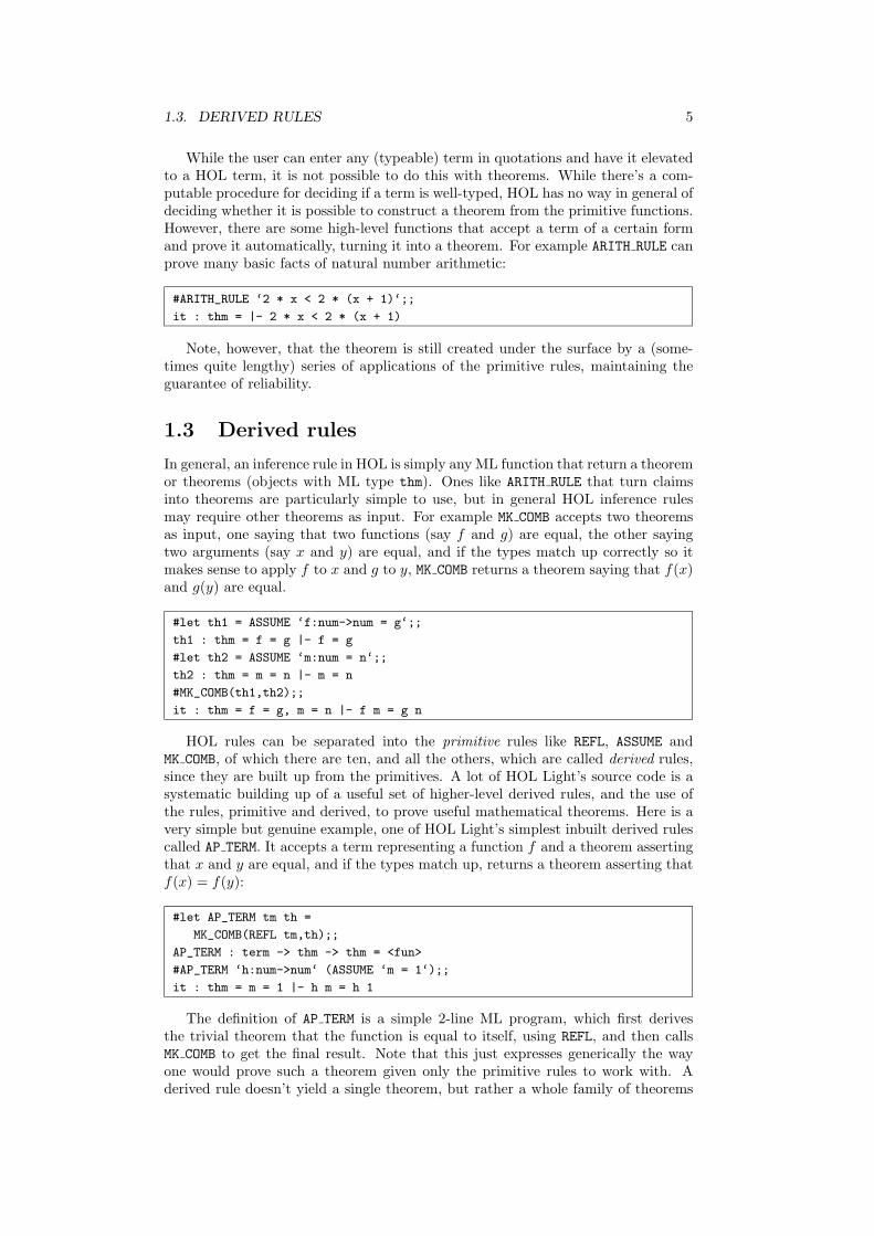
While the user can enter any (typeable) term in quotations and have it elevatedto a HOL term, it is not possible to do this with theorems. While there’s a com-putable procedure for deciding if a term is well-typed, HOL has no way in general ofdeciding whether it is possible to construct a theorem from the primitive functions.However, there are some high-level functions that accept a term of a certain formand prove it automatically, turning it into a theorem. For example ARITH RULE canprove many basic facts of natural number arithmetic:
#ARITH_RULE ‘2 * x < 2 * (x + 1)‘;;
it : thm = |- 2 * x < 2 * (x + 1)
Note, however, that the theorem is still created under the surface by a (some-times quite lengthy) series of applications of the primitive rules, maintaining theguarantee of reliability.
1.3 Derived rules
In general, an inference rule in HOL is simply any ML function that return a theoremor theorems (objects with ML type thm). Ones like ARITH RULE that turn claimsinto theorems are particularly simple to use, but in general HOL inference rulesmay require other theorems as input. For example MK COMB accepts two theoremsas input, one saying that two functions (say f and g) are equal, the other sayingtwo arguments (say x and y) are equal, and if the types match up correctly so itmakes sense to apply f to x and g to y, MK COMB returns a theorem saying that f(x)and g(y) are equal.
#let th1 = ASSUME ‘f:num->num = g‘;;
th1 : thm = f = g |- f = g
#let th2 = ASSUME ‘m:num = n‘;;
th2 : thm = m = n |- m = n
#MK_COMB(th1,th2);;
it : thm = f = g, m = n |- f m = g n
HOL rules can be separated into the primitive rules like REFL, ASSUME andMK COMB, of which there are ten, and all the others, which are called derived rules,since they are built up from the primitives. A lot of HOL Light’s source code is asystematic building up of a useful set of higher-level derived rules, and the use ofthe rules, primitive and derived, to prove useful mathematical theorems. Here is avery simple but genuine example, one of HOL Light’s simplest inbuilt derived rulescalled AP TERM. It accepts a term representing a function f and a theorem assertingthat x and y are equal, and if the types match up, returns a theorem asserting thatf(x) = f(y):
#let AP_TERM tm th =
MK_COMB(REFL tm,th);;
AP_TERM : term -> thm -> thm = <fun>
#AP_TERM ‘h:num->num‘ (ASSUME ‘m = 1‘);;
it : thm = m = 1 |- h m = h 1
The definition of AP TERM is a simple 2-line ML program, which first derivesthe trivial theorem that the function is equal to itself, using REFL, and then callsMK COMB to get the final result. Note that this just expresses generically the wayone would prove such a theorem given only the primitive rules to work with. Aderived rule doesn’t yield a single theorem, but rather a whole family of theorems
6 CHAPTER 1. INTRODUCTION
depending on the input. It corresponds naturally to what a logician would think ofas a ‘derived rule’.
CAML Light, described in the next Part, is a full programming language, soone can perform essentially any kinds of inference one wants, provided it is reducedto the existing infrastructure of primitive and derived rules. Derived rules oftenhave a recursive structure, passing over the input term and transforming it into anappropriate theorem. They may also do different things depending, for example, onthe logical structure of the input, the names of variables, and so on. All this willbe illustrated in more detail in what follows.
Further reading
The original textbook on Edinburgh LCF by Gordon, Milner, and Wadsworth (1979)introduces many of the basic ideas in HOL Light; see also the later book by Paul-son (1987) on a re-engineered version ‘Cambridge LCF’. The general approach totheorem-proving described above is, as emphasized by Gordon (1982), largely in-dependent of the particular logic one works with, e.g. the original LCF (logic ofcomputable functions), higher order logic, or first order set theory. The originalHOL was born when Gordon used the Cambridge LCF system to implement clas-sical higher order logic. There is a book by Gordon and Melham (1993) describingan early version of the system ‘HOL88’, while an interesting historical survey ofthe development of LCF and HOL is given by Gordon (2000). The original ML isalso described in the early LCF publications. CAML Light has extensive on-linedocumentation and a book (in French) by Weis and Leroy (1993) devoted to it.Another ML version, Standard ML, is described by Paulson (1991).

Part I
CAML tutorial
7


Chapter 2
A taste of CAML
CAML Light feels rather different from common programming languages like C orFORTRAN. The major difference is that it is a functional rather than imperativelanguage. While it does have imperative features, we won’t make very great useof them. The following section explains the contrast; readers with no previousprogramming experience may choose to skip or just skim this material.
2.1 Imperative vs functional programming
Programs in traditional languages, such as FORTRAN, Algol, C and Modula-3,rely heavily on modifying the values of a collection of variables, called the state.Before execution, the state has some initial value σ, representing the inputs tothe program, and when the program has finished, the state has a new value σ′
including the result(s). During execution, each command changes the state, whichhas therefore proceeded through some finite sequence of values:
σ = σ0 → σ1 → σ2 → · · · → σn = σ′
For example in a sorting program, the state initially includes an array of values,and when the program has finished, the state has been modified in such a way thatthese values are sorted, while the intermediate states represent progress towardsthis goal.
The state is typically modified by assignment commands, often written in theform v = E or v := E where v is a variable and E some expression. These commandscan be executed in a sequential manner by writing them one after the other in theprogram, often separated by a semicolon. By using statements like if and while,one can execute these commands conditionally, and repeatedly, depending on otherproperties of the current state. The program amounts to a set of instructions onhow to perform these state changes, and therefore this style of programming is oftencalled imperative or procedural. Correspondingly, the traditional languages intendedto support it are known as imperative or procedural languages.
Functional programming represents a radical departure from this model. Essen-tially, a functional program is simply an expression, and execution means evaluationof the expression.1 We can see how this might be possible, in general terms, as fol-lows. Assuming that an imperative program (as a whole) is deterministic, i.e. theoutput is completely determined by the input, we can say that the final state, orwhichever fragments of it are of interest, is some function of the initial state, say
1Functional programming is often called ‘applicative programming’ since the basic mechanismis the application of functions to arguments.
9

10 CHAPTER 2. A TASTE OF CAML
σ′ = f(σ).2 In functional programming this view is emphasized: the program isactually an expression that corresponds to the mathematical function f . Functionallanguages support the construction of such expressions by allowing rather powerfulfunctional constructs.
Functional programming can be contrasted with imperative programming eitherin a negative or a positive sense. Negatively, pure functional programs do not usevariables — there is no state. Consequently, they cannot use assignments, sincethere is nothing to assign to. Furthermore the idea of executing commands in se-quence is meaningless, since the first command can make no difference to the second,there being no state to mediate between them. Positively however, functional pro-grams can use functions in much more sophisticated ways. Functions can be treatedin exactly the same way as simpler objects like integers: they can be passed to otherfunctions as arguments and returned as results, and in general calculated with. In-stead of sequencing and looping, functional languages use recursive functions, i.e.functions that are defined in terms of themselves. By contrast, most traditional lan-guages provide poor facilities in these areas. C allows some limited manipulation offunctions via pointers, but does not allow one to create new functions dynamically.FORTRAN does not even support recursion at all.
A potential advantage of functional languages is the following. Since the eval-uation of expressions has no side-effect on any state, separate subexpressions canbe evaluated in any order without affecting each other. This makes programs morecomprehensible and debugging easier, since there is no danger of one part of aprogram unexpectedly affecting others. Moreover, functional programs may lendthemselves well to parallel implementation, i.e. the computer can automaticallyfarm out different subexpressions to different processors. By contrast, imperativeprograms often impose a fairly rigid order of execution, and even the limited inter-leaving of instructions in modern pipelined processors turns out to be complicatedand full of technical problems.
Actually, CAML is not a purely functional programming language; it does havevariables and assignments if required. Most of the time, we will work inside thepurely functional subset. But even when we do use assignments, and lose some ofthe preceding benefits, there are advantages in the more flexible use of functionsthat languages like CAML allow. Programs can often be expressed in a very con-cise and elegant style using higher-order functions (functions that operate on otherfunctions). Code can be made more general, since it can be parametrized even overother functions. For example, a program to add up a list of numbers and a pro-gram to multiply a list of numbers can be seen as instances of the same program,parametrized by the pairwise arithmetic operation and the corresponding identity.In one case it is given + and 0 and in the other case, ∗ and 1.
2.2 Basic use of CAML
We will use CAML in its interactive and interpretive mode. When it is started itpresents its prompt (‘#’):
> Caml Light version 0.74
#
(In order to exit the system, simply type ctrl/d or quit();; at the prompt.)When CAML presents you with its prompt, you can type in expressions, terminated
2Compare Naur’s remarks (Raphael 1966) that he can write any program in a single statementOutput = Program(Input).

2.2. BASIC USE OF CAML 11
by two successive semicolons, and it will evaluate them and print the result. Incomputing jargon, the CAML system sits in a read-eval-print loop: it repeatedlyreads an expression, evaluates it, and prints the result. For example, CAML can beused as a simple calculator:
#10 + 5;;
it : int = 15
The system not only returns the answer, but also the type of the expression,which it has inferred automatically. (We will have more to say about CAML’stypes in a later section.) It can do this because it knows the type of the built-inaddition operator +. On the other hand, if an expression is not typable, the systemwill reject it, and try to give some idea about how the types fail to match up. Incomplicated cases, the error messages can be quite tricky to understand.
#1 + true;;
Toplevel input:
>let it = 1 + true;;
> ^^^^
This expression has type bool,
but is used with type int.
Since CAML is a functional language, expressions are allowed to be functions.Functions can be written in CAML using the syntax fun x -> t[x] for the functionthat maps an argument x to t[x], the latter being any expression involving x. Suchan expression involving ‘fun x -> ...’ is said to be a function abstraction. Forexample we can define the successor function:
#fun x -> x + 1;;
it : int -> int = <fun>
Again, the type of the expression, this time int -> int, meaning a functionfrom integers to integers, is inferred and displayed. However the function itselfis not printed; the system merely writes <fun>. This is because, in general, theinternal representations of functions are not very readable.3 In normal mathematicalnotation, application of a function f to an argument x is written f(x). In CAML,the parentheses can be omitted unless they are needed to enforce grouping, e.g.
#(fun x -> x + 1) 1 * 2;;
it : int = 4
#(fun x -> x + 1) (1 * 2);;
it : int = 3
#((fun x -> x + 1) 1) * 2;;
it : int = 4
Every function in CAML takes just a single argument. However there are twoways of getting the effect of functions of more than one argument. One way isto have a single argument but of a more complex type, such as pairs (see later)of integers. The other is to use ‘currying’ (after the logical Haskell Curry), wherethe function takes one argument and yields another function that takes the secondargument, and so on. For example, a curried function of two arguments that addsthe arguments together can be written and used as follows:
3CAML does not store them simply as syntax trees, but compiles them into bytecode.
12 CHAPTER 2. A TASTE OF CAML
#fun x -> (fun y -> x + y);;
it : int -> int -> int = <fun>
#(fun x -> (fun y -> x + y)) 1;;
it : int -> int = <fun>
#((fun x -> (fun y -> x + y)) 1) 2;;
it : int = 3
Note that the function has type int -> int -> int, meaning int -> (int ->int). When applied to one argument, 1, it yields another function, which takes thesecond argument and maps it to the corresponding sum. Currying is used a lot infunctional programming, since it allows functions to be used quite flexibly. Someother syntactic conventions support it; for example, without parentheses to enforcegrouping, function application associates to the left, i.e. f g x means (f g)(x) notf(g(x)). We can write the above example more succinctly as:
#(fun x y -> x + y) 1 2;;
it : int = 3
2.3 Bindings and declarations
A nontrivial functional program is a very complex expression, and it is of coursenot convenient to evaluate it all in one go. Instead, useful subexpressions can beevaluated and bound to names using let. (In fact, a filter in front of CAML Light,part of HOL Light, automatically binds the last anonymous expression evaluatedto the special name it, hence its appearance above.) For example:
#let successor = fun x -> x + 1;;
successor : int -> int = <fun>
#successor 5;;
it : int = 6
Declarations can be made local to the evaluation of an expression, so they areinvisible afterwards, using in. For example:
#let suc = fun x -> x + 1 in
suc(suc 1);;
it : int = 3
#suc 1;;
Toplevel input:
>let it = suc 1;;
> ^^^
The value identifier suc is unbound.
The arguments to functions can be written on the left of the equation, whichmost people find more natural:
#let successor x = x + 1;;
successor : int -> int = <fun>
#successor 5;;
it : int = 6
Functions can be recursive, i.e. defined in terms of themselves. To achieve this,simply include the keyword rec. For example, the factorial n! = 1×2×· · ·×(n−1)×ncan be evaluated as follows: evaluate (n− 1)! recursively, then multiply by n:
2.3. BINDINGS AND DECLARATIONS 13
#let rec fact n = if n = 0 then 1
else n * fact(n - 1);;
fact : int -> int = <fun>
#fact 6;;
it : int = 720
By using and, one can make several binding simultaneously, and define mutuallyrecursive functions. For example, here are two simple, though highly inefficient,functions to decide whether or not a natural number is odd or even:
#let rec even n = if n = 0 then true else odd (n - 1)
and odd n = if n = 0 then false else even (n - 1);;
even : int -> bool = <fun>
odd : int -> bool = <fun>
#even 12;;
it : bool = true
#odd 14;;
it : bool = false
If declarations do not include the rec keyword, then any instance of the namecurrently being bound on the right is taken to be the previous value. For example:
#let successor n = successor(successor n);;
successor : int -> int = <fun>
#successor 2;;
it : int = 4
#successor 5;;
it : int = 7
The old binding is now overwritten. But note that we are not making assign-ments to variables. Each binding is only done once when the system analyses theinput; it cannot be repeated or modified. It can be overwritten by a new defini-tion using the same name, but this is not assignment in the usual sense, since thesequence of events is only connected with the compilation process, not with thedynamics of program execution. Indeed, apart from the more interactive feedbackfrom the system, we could equally replace all the double semicolons after the dec-larations by in and evaluate everything at once. On this view we can see that theoverwriting of a declaration really corresponds to the definition of a new local vari-able that hides the outer one, according to the scoping rules usual in programminglanguages. For example:
#let x = 1;;
x : int = 1
#let y = 2;;
y : int = 2
#let x = 3;;
x : int = 3
#x + y;;
- : int = 5
is the same as:
#let x = 1 in
let y = 2 in
let x = 3 in
x + y;;
- : int = 5

14 CHAPTER 2. A TASTE OF CAML
Note carefully that variable binding is static, i.e. the first binding of x is stillused until an inner binding occurs, and any uses of it until that point are not affectedby the inner binding.4 For example:
#let x = 1;;
x : int = 1
#let f w = w + x;;
f : int -> int = <fun>
#let x = 2;;
x : int = 2
#f 0;;
it : int = 1
2.4 Evaluation rules
In essence, CAML is quite simple to understand, since it just evaluates expressions.However there are subtle questions over the precise order of evaluation. For example,consider the following recursive function:
#let rec f x = f(x + 1);;
f : int -> ’a = <fun>
#f 2;;
Interrupted.
Evaluation of f 2 looped indefinitely, until interrupted by ctrl/c. Now supposewe use f in another expression, but in a way that doesn’t require f to be evaluatedon any arguments:
#(fun x -> 1) (f 2);;
Interrupted.
Even so, an indefinite loop results. The reason is that according to CAML’sevaluation rules, all arguments to a function are evaluated before being insertedin the function body. This strategy is called eager, in contrast to cleverer lazyapproaches that try to avoid evaluating subexpressions until they are definitelyneeded (and then no more than once).
CAML adopts eager evaluation for two main reasons. Choreographing the reduc-tions and sharings that occur in lazy evaluation is quite tricky, and implementationstend to be relatively inefficient and complicated. Unless the programmer is verycareful, memory can fill up with pending unevaluated expressions, and in generalit is hard to understand the space behaviour of programs. In fact many imple-mentations of lazy evaluation try to optimize it to eager evaluation in cases wherethere is no semantic difference. By contrast, in CAML, we always first evaluate thearguments to functions and only then inserts them in the body — this is simpleand efficient, and is easy to implement using standard compiler technology.
The second reason for preferring eager evaluation is that CAML is not a purefunctional language, but includes imperative features (variables, assignments etc.).Therefore the order of evaluation of subexpressions can make a big difference. Iflazy evaluation is used, it seems to become difficult for the programmer to visualize,
4The first version of LISP used dynamic binding, where a rebinding of a variable propagated toearlier uses of the variable. This was in fact originally regarded as a bug, but soon programmersstarted to appreciate its convenience. The feature survived for a long time in many LISP dialects,but eventually the view that static binding is better prevailed. In Common LISP, static bindingis the default, but dynamic binding is available if desired via the keyword special.
2.5. TYPES AND POLYMORPHISM 15
in a nontrivial program, exactly when each subexpression gets evaluated. In theeager CAML system, one just needs to remember the simple evaluation rules. Tobe explicit, they are as follows:
• Constants (e.g. predefined values and functions like 1 and +) evaluate tothemselves.
• Evaluation stops immediately at expressions of the form fun x -> ..., anddoes not look inside them. This only happens when such an expression isapplied to an argument.
• When evaluating an application s t, then first both s and t are evaluated.5
Then, assuming that the evaluated form of s is a function fun x -> ..., thebody is evaluated with each instance of x replaced by the evaluated form oft. If the evaluated form of s is a built-in function like +, the appropriateevaluation is performed.
• When evaluating if E1 then E2 else E3, first E1 is evaluated, and depend-ing on whether it yields true or false, either E2 or E3 respectively (and notthe other) is evaluated.
One can regard let x = E1 in E2 as an abbreviation for (fun x -> E2) E1,and the above evaluation rules then give the right answer: E1 is evaluated, and thenthe evaluated form replaces each x in E1, which is then itself evaluated. Let us seesome examples of evaluating expressions:
(fun x -> (fun y -> y + y) x) (2 + 2)= (fun x -> (fun y -> y + y) x) 4= (fun y -> y + y) 4= 4 + 4= 8
Note that the subterm (fun y -> y + y) x is not reduced, since it is inside thefunction abstraction ‘fun x -> ...’. However, terms that are reducible and not soenclosed in both function and argument get reduced before the function applicationitself is evaluated, e.g. the second step in the following:
((fun f x -> f x) (fun y -> y + y)) (2 + 2)= ((fun f x -> f x) (fun y -> y + y)) 4= (fun x -> (fun y -> y + y) x) 4= (fun y -> y + y) 4= 4 + 4= 8
The fact that CAML does not evaluate under function abstractions is of crucialimportance to advanced programmers. It gives precise control over the evaluation ofexpressions, and can be used to mimic many of the helpful cases of lazy evaluation,or sometimes to force earlier evaluation of expressions by moving them outside funx -> ....
2.5 Types and polymorphism
Some functions do not have a fixed type. For example, the identity function thatreturns its argument unchanged doesn’t care whether its argument is an integer, a
5CAML Light actually evaluates t first.
16 CHAPTER 2. A TASTE OF CAML
boolean, or another function. Therefore, it is said to have polymorphic type, andCAML displays a type involving type variables. These can later be set to someparticular type when it is used, different instances with different types.
#let I = fun x -> x;;
I : ’a -> ’a = <fun>
CAML prints type variables as ’a, ’b etc.; these are supposed to be ASCIIrepresentations of α, β and so on. We can now use the polymorphic functionseveral times with different types:
#I true;;
- : bool = true
#I 1;;
- : int = 1
#I I I I 12;;
- : int = 12
Each instance of I in the last expression has a different type, and intuitivelycorresponds to a different function. CAML always assigns the most general typepossible for an expression, without specializing it unnecessarily, using an algorithmdue to Milner (1978). For example, the following is a more complex definition of anidentity function; the reader may wish to study it to see why CAML gives all theseexpressions the types it does,6 and why I’ acts as an identity function. Note thatin contrast to most programming languages, CAML allows the prime character invariable names, reflecting its background in logic and mathematics where variableslike x′ are common.
#let K x y = x;;
K : ’a -> ’b -> ’a = <fun>
#let S f g x = (f x) (g x);;
S : (’a -> ’b -> ’c) -> (’a -> ’b) -> ’a -> ’c = <fun>
#let I’ = S K K;;
I’ : ’_a -> ’_a = <fun>
#I’ 2;;
it : int = 2
In the above examples of polymorphic functions, the system very quickly infers amost general type for each expression, and the type it infers is simple. This usuallyhappens in practice, but there are pathological cases, e.g. the following example dueto Mairson (1990). The type of this expression takes about 10 seconds to calculate,and occupies over 4000 lines on an 80-column terminal.
let pair x y = fun z -> z x y in
let x1 = fun y -> pair y y in
let x2 = fun y -> x1(x1 y) in
let x3 = fun y -> x2(x2 y) in
let x4 = fun y -> x3(x3 y) in
let x5 = fun y -> x4(x4 y) in
x5(fun z -> z);;
Because of CAML’s automatic type inference, the programmer need never entera type. At least, CAML will already allocate as general a type as possible to an
6Ignore the underscores for now. This is connected with the typing of imperative features, andwe will discuss it later.

2.6. EQUALITY OF FUNCTIONS 17
expression. However it may sometimes be convenient to restrict the generality ofa type. This cannot make code work that didn’t work before, but it may serve asdocumentation regarding the intended purpose of the code; it is also possible touse shorter synonyms for complicated types. Type restriction can be achieved inCAML by adding type annotations after some expression(s). These type annotationsconsist of a colon followed by a type. It usually doesn’t matter exactly wherethese annotations are added, provided they enforce the appropriate constraints.For example, here are some alternative ways of constraining the identity functionto type int -> int:
#let I (x:int) = x;;
I : int -> int = <fun>
#let I x = (x:int);;
I : int -> int = <fun>
#let (I:int->int) = fun x -> x;;
I : int -> int = <fun>
#let I = fun (x:int) -> x;;
I : int -> int = <fun>
#let I = ((fun x -> x):int->int);;
I : int -> int = <fun>
2.6 Equality of functions
Instead of comparing the actions of I and I ′ on particular arguments like 3, itwould seem that we can settle the matter definitively by comparing the functionsthemselves. However this doesn’t work:
#I’ = I;;
Uncaught exception: Invalid_argument "equal: functional value"
It is in general forbidden to compare functions for equality, though a few specialinstances, where the functions are obviously the same, yield true:
#let f x = x + 1;;
f : int -> int = <fun>
#let g x = x + 1;;
g : int -> int = <fun>
#f = f;;
it : bool = true
#f = g;;
Uncaught exception: Invalid_argument "equal: functional value"
#let h = g;;
h : int -> int = <fun>
#h = f;;
Uncaught exception: Invalid_argument "equal: functional value"
#h = g;;
it : bool = true
Why these restrictions? Aren’t functions supposed to be first-class objects inCAML? Yes, but unfortunately, (extensional) function equality is not computable.This follows from a number of classic theorems in recursion theory, such as theunsolvability of the halting problem and Rice’s theorem.7 Let us give a concrete
7Rice’s theorem is an extremely strong undecidability result which asserts that any nontrivialproperty of the function corresponding to a program is uncomputable from its text. An excellentcomputation theory textbook is Davis, Sigal, and Weyuker (1994).

18 CHAPTER 2. A TASTE OF CAML
illustration of why this might be so. It is still an open problem whether the followingfunction terminates for all arguments, the assertion that it does being known as theCollatz conjecture:8
#let rec collatz n =
if n <= 1 then 0
else if even(n) then collatz(n / 2)
else collatz(3 * n + 1);;
collatz : int -> int = <fun>
What is clear, though, is that if it does halt it returns 0. Now consider thefollowing trivial function:
#let f (x:int) = 0;;
f : int -> int = <fun>
By deciding the equation collatz = f, the computer would settle the Collatzconjecture. It is easy to concoct other examples for open mathematical problems.
It is possible to trap out applications of the equality operator to functions anddatatypes built up from them as part of typechecking, rather than at runtime. Thisis the approach taken by Standard ML. Types that do not involve functions inthese ways are known as equality types, since it is always valid to test objects ofsuch types for equality. On the negative side, this makes the type system muchmore complicated. However one might argue that static typechecking should beextended as far as feasibility allows.
Further reading
Numerous textbooks on ‘functional programming’ include a general introductionto the field and a contrast with imperative programming — browse through a fewand find one that you like. A detailed and polemical advocacy of the functionalstyle is given by Backus (1978), the main inventor of FORTRAN. A good elementaryintroduction to CAML Light and functional programming is Mauny (1995). Paulson(1991) is another good textbook, though based on Standard ML.
8A good survey of this problem, and attempts to solve it, is given by Lagarias (1985). Strictly,we should use unlimited precision integers rather than machine arithmetic. We will see later howto do this.
Chapter 3
Further CAML
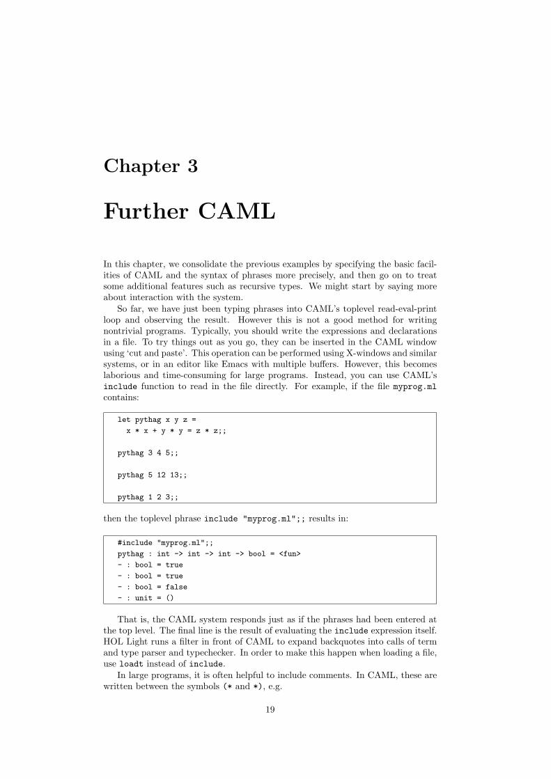
In this chapter, we consolidate the previous examples by specifying the basic facil-ities of CAML and the syntax of phrases more precisely, and then go on to treatsome additional features such as recursive types. We might start by saying moreabout interaction with the system.
So far, we have just been typing phrases into CAML’s toplevel read-eval-printloop and observing the result. However this is not a good method for writingnontrivial programs. Typically, you should write the expressions and declarationsin a file. To try things out as you go, they can be inserted in the CAML windowusing ‘cut and paste’. This operation can be performed using X-windows and similarsystems, or in an editor like Emacs with multiple buffers. However, this becomeslaborious and time-consuming for large programs. Instead, you can use CAML’sinclude function to read in the file directly. For example, if the file myprog.mlcontains:
let pythag x y z =
x * x + y * y = z * z;;
pythag 3 4 5;;
pythag 5 12 13;;
pythag 1 2 3;;
then the toplevel phrase include "myprog.ml";; results in:
#include "myprog.ml";;
pythag : int -> int -> int -> bool = <fun>
- : bool = true
- : bool = true
- : bool = false
- : unit = ()
That is, the CAML system responds just as if the phrases had been entered atthe top level. The final line is the result of evaluating the include expression itself.HOL Light runs a filter in front of CAML to expand backquotes into calls of termand type parser and typechecker. In order to make this happen when loading a file,use loadt instead of include.
In large programs, it is often helpful to include comments. In CAML, these arewritten between the symbols (* and *), e.g.
19

20 CHAPTER 3. FURTHER CAML
(* ------------------------------------------------------ *)
(* This function tests if (x,y,z) is a Pythagorean triple *)
(* ------------------------------------------------------ *)
let pythag x y z =
x * x + y * y = z * z;;
(*comments*) pythag (*can*) 3 (*go*) 4 (*almost*) 5 (*anywhere*)
(* and (* can (* be (* nested *) quite *) arbitrarily *) *);;
3.1 Basic datatypes and operations
CAML features several built-in primitive types. From these, composite types maybe built using various type constructors. For the moment, we will only use thefunction space constructor -> and the Cartesian product constructor *, but we willsee in due course which others are provided, and how to define new types and typeconstructors. The primitive types that concern us now are:
• The type unit. This is a 1-element type, whose only element is written ().Obviously, something of type unit conveys no information, so it is commonlyused as the return type of imperatively written ‘functions’ that perform aside-effect, such as include above. It is also a convenient argument wherethe only use of a function type is to delay evaluation.
• The type bool. This is a 2-element type of booleans (truth-values) whoseelements are written true and false.
• The type int. This contains some finite subset of the positive and negativeintegers. Typically the permitted range is from −230 (−1073741824) up to230− 1 (1073741823).1 The numerals are written in the usual way, optionallywith a negation sign, e.g. 0, 32, -25.
• The type string contains strings (i.e. finite sequences) of characters. Theyare written and printed between double quotes, e.g. "hello". In order toencode include special characters in strings, C-like escape sequences are used.For example, \" is the double quote itself, and \n is the newline character.
The above values like (), false, 7 and "caml" are all to be regarded as fixedconstants. There are other constants corresponding to operations on the basic types.Some of these may be written as infix operators, for the sake of familiarity. Thesehave a notion of precedence so that expressions are grouped together as one wouldexpect. For example, we write x + y rather than + x y and x < 2 * y + z ratherthan < x (+ (* 2 y) z). The logical operator not also has a special parsingstatus, in that the usual left-associativity rule is reversed for it: not not p meansnot (not p). User-defined functions may be granted infix status via the #infixdirective. For example, here is a definition of a function performing composition offunctions:
1We will see later how to use an alternative type of integers with unlimited precision.
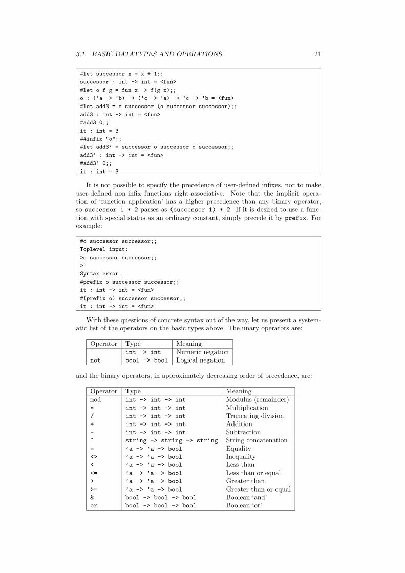
3.1. BASIC DATATYPES AND OPERATIONS 21
#let successor x = x + 1;;
successor : int -> int = <fun>
#let o f g = fun x -> f(g x);;
o : (’a -> ’b) -> (’c -> ’a) -> ’c -> ’b = <fun>
#let add3 = o successor (o successor successor);;
add3 : int -> int = <fun>
#add3 0;;
it : int = 3
##infix "o";;
#let add3’ = successor o successor o successor;;
add3’ : int -> int = <fun>
#add3’ 0;;
it : int = 3
It is not possible to specify the precedence of user-defined infixes, nor to makeuser-defined non-infix functions right-associative. Note that the implicit opera-tion of ‘function application’ has a higher precedence than any binary operator,so successor 1 * 2 parses as (successor 1) * 2. If it is desired to use a func-tion with special status as an ordinary constant, simply precede it by prefix. Forexample:
#o successor successor;;
Toplevel input:
>o successor successor;;
>^
Syntax error.
#prefix o successor successor;;
it : int -> int = <fun>
#(prefix o) successor successor;;
it : int -> int = <fun>
With these questions of concrete syntax out of the way, let us present a system-atic list of the operators on the basic types above. The unary operators are:
Operator Type Meaning- int -> int Numeric negationnot bool -> bool Logical negation
and the binary operators, in approximately decreasing order of precedence, are:
Operator Type Meaningmod int -> int -> int Modulus (remainder)* int -> int -> int Multiplication/ int -> int -> int Truncating division+ int -> int -> int Addition- int -> int -> int Subtraction^ string -> string -> string String concatenation= ’a -> ’a -> bool Equality<> ’a -> ’a -> bool Inequality< ’a -> ’a -> bool Less than<= ’a -> ’a -> bool Less than or equal> ’a -> ’a -> bool Greater than>= ’a -> ’a -> bool Greater than or equal& bool -> bool -> bool Boolean ‘and’or bool -> bool -> bool Boolean ‘or’
22 CHAPTER 3. FURTHER CAML
For example, x > 0 & x < 1 is parsed as & (> x 0) (< x 1). Note that all thecomparisons, not just the equality relation, are polymorphic. They not only orderintegers in the expected way, and strings alphabetically, but all other primitivetypes and composite types in a fairly natural way. Once again, however, they arenot in general allowed to be used on functions.
The two boolean operations & and or have their own special evaluation strategy,like the conditional expression. In fact, they can be regarded as synonyms forconditional expressions:
p & q4= if p then q else false
p or q4= if p then true else q
Thus, the ‘and’ operation evaluates its first argument, and only if it is true,evaluates its second. Conversely, the ‘or’ operation evaluates its first argument,and only if it is false evaluates its second.
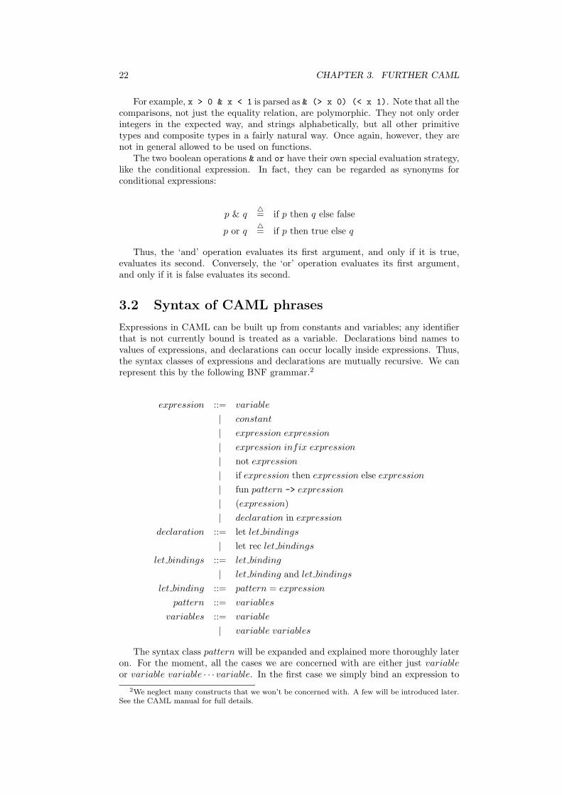
3.2 Syntax of CAML phrases
Expressions in CAML can be built up from constants and variables; any identifierthat is not currently bound is treated as a variable. Declarations bind names tovalues of expressions, and declarations can occur locally inside expressions. Thus,the syntax classes of expressions and declarations are mutually recursive. We canrepresent this by the following BNF grammar.2
expression ::= variable
| constant
| expression expression
| expression infix expression
| not expression| if expression then expression else expression| fun pattern -> expression
| (expression)| declaration in expression
declaration ::= let let bindings| let rec let bindings
let bindings ::= let binding
| let binding and let bindingslet binding ::= pattern = expression
pattern ::= variables
variables ::= variable
| variable variables
The syntax class pattern will be expanded and explained more thoroughly lateron. For the moment, all the cases we are concerned with are either just variableor variable variable · · · variable. In the first case we simply bind an expression to
2We neglect many constructs that we won’t be concerned with. A few will be introduced later.See the CAML manual for full details.
3.3. FURTHER EXAMPLES 23
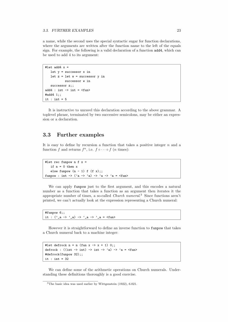
a name, while the second uses the special syntactic sugar for function declarations,where the arguments are written after the function name to the left of the equalssign. For example, the following is a valid declaration of a function add4, which canbe used to add 4 to its argument:
#let add4 x =
let y = successor x in
let z = let w = successor y in
successor w in
successor z;;
add4 : int -> int = <fun>
#add4 1;;
it : int = 5
It is instructive to unravel this declaration according to the above grammar. Atoplevel phrase, terminated by two successive semicolons, may be either an expres-sion or a declaration.
3.3 Further examples
It is easy to define by recursion a function that takes a positive integer n and afunction f and returns fn, i.e. f ◦ · · · ◦ f (n times):
#let rec funpow n f x =
if n = 0 then x
else funpow (n - 1) f (f x);;
funpow : int -> (’a -> ’a) -> ’a -> ’a = <fun>
We can apply funpow just to the first argument, and this encodes a naturalnumber as a function that takes a function as an argument then iterates it theappropriate number of times, a so-called Church numeral.3 Since functions aren’tprinted, we can’t actually look at the expression representing a Church numeral:
#funpow 6;;
it : (’_a -> ’_a) -> ’_a -> ’_a = <fun>
However it is straightforward to define an inverse function to funpow that takesa Church numeral back to a machine integer:
#let defrock n = n (fun x -> x + 1) 0;;
defrock : ((int -> int) -> int -> ’a) -> ’a = <fun>
#defrock(funpow 32);;
it : int = 32
We can define some of the arithmetic operations on Church numerals. Under-standing these definitions thoroughly is a good exercise.
3The basic idea was used earlier by Wittgenstein (1922), 6.021.
24 CHAPTER 3. FURTHER CAML
#let add m n f x = m f (n f x);;
add : (’a -> ’b -> ’c) -> (’a -> ’d -> ’b) -> ’a -> ’d -> ’c = <fun>
#let mul m n f x = m (n f) x;;
mul : (’a -> ’b -> ’c) -> (’d -> ’a) -> ’d -> ’b -> ’c = <fun>
#let exp m n f x = n m f x;;
exp : ’a -> (’a -> ’b -> ’c -> ’d) -> ’b -> ’c -> ’d = <fun>
#let test bop x y = defrock (bop (funpow x) (funpow y));;
test :
(((’a -> ’a) -> ’a -> ’a) ->
((’b -> ’b) -> ’b -> ’b) -> (int -> int) -> int -> ’c) ->
int -> int -> ’c = <fun>
#test add 2 10;;
it : int = 12
#test mul 2 10;;
it : int = 20
#test exp 2 10;;
it : int = 1024
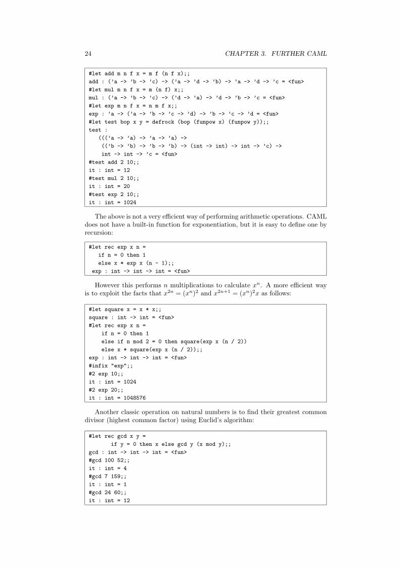
The above is not a very efficient way of performing arithmetic operations. CAMLdoes not have a built-in function for exponentiation, but it is easy to define one byrecursion:
#let rec exp x n =
if n = 0 then 1
else x * exp x (n - 1);;
exp : int -> int -> int = <fun>
However this performs n multiplications to calculate xn. A more efficient wayis to exploit the facts that x2n = (xn)2 and x2n+1 = (xn)2x as follows:
#let square x = x * x;;
square : int -> int = <fun>
#let rec exp x n =
if n = 0 then 1
else if n mod 2 = 0 then square(exp x (n / 2))
else x * square(exp x (n / 2));;
exp : int -> int -> int = <fun>
#infix "exp";;
#2 exp 10;;
it : int = 1024
#2 exp 20;;
it : int = 1048576
Another classic operation on natural numbers is to find their greatest commondivisor (highest common factor) using Euclid’s algorithm:
#let rec gcd x y =
if y = 0 then x else gcd y (x mod y);;
gcd : int -> int -> int = <fun>
#gcd 100 52;;
it : int = 4
#gcd 7 159;;
it : int = 1
#gcd 24 60;;
it : int = 12

3.4. TYPE DEFINITIONS 25
Rather than using the rec keyword every time we declare a recursive function,eccentrics might prefer to define a recursion operator Rec, and thereafter use that,e.g.
#let rec Rec f = f(fun x -> Rec f x);;
Rec : ((’a -> ’b) -> ’a -> ’b) -> ’a -> ’b = <fun>
#let fact = Rec (fun f n -> if n = 0 then 1 else n * f(n - 1));;
fact : int -> int = <fun>
#fact 3;;
it : int = 6
Note, however, that the function abstraction ‘fun x -> ...’ in the definitionwas essential, otherwise the expression Rec f goes into an infinite recursion whenevaluated, before it is even applied to its argument:
#let rec Rec f = f(Rec f);;
Rec : (’a -> ’a) -> ’a = <fun>
#let fact = Rec (fun f n -> if n = 0 then 1 else n * f(n - 1));;
Uncaught exception: Out_of_memory
3.4 Type definitions
CAML has facilities for declaring new type constructors, so that composite types canbe built up out of existing ones. In fact, CAML goes further and allows a compositetype to be built up not only out of preexisting types but also from the compositetype itself. Such types, naturally enough, are said to be recursive, even if they don’tavail themselves of the chance to use the type being defined in the definition. Theyare declared using the type keyword followed by an equation indicating how thenew type is built up from existing ones and itself. We will illustrate this by a fewexamples. The first one is the definition of a sum type, intended to correspond tothe disjoint union of two existing types.
#type (’a,’b)sum = inl of ’a | inr of ’b;;
Type sum defined.
Roughly, an object of type (’a,’b)sum is either something of type ’a or some-thing of type ’b. More formally, however, all these things have different types.The type declaration also declares the so-called constructors inl and inr. Theseare functions that take objects of the component types and inject them into thenew type. Indeed, we can see their types in the CAML system and apply them toobjects:
#inl;;
it : ’a -> (’a, ’b) sum = <fun>
#inr;;
it : ’a -> (’b, ’a) sum = <fun>
#inl 5;;
it : (int, ’a) sum = inl 5
#inr false;;
it : (’a, bool) sum = inr false
We can visualize the situation via the following diagram. Given two existingtypes α and β, the type (α, β)sum is composed precisely of separate copies of αand β, and the two constructors map onto the respective copies:

26 CHAPTER 3. FURTHER CAML
α
β
(α, β)sum
������
������
�:
inl
inr
XXXXXXXXXXXXXz
This is similar to a union in C, but in CAML the copies of the component typesare kept apart and one always knows which of these an element of the union belongsto. By contrast, in C the component types are overlapped, and the programmer isresponsible for this book-keeping.
3.4.1 Pattern matching
The constructors in such a definition have three very important properties:
• They are exhaustive, i.e. every element of the new type is obtainable eitherby inl x for some x or inr y for some y. That is, the new type containsnothing besides copies of the component types.
• They are injective, i.e. an equality test inl x = inl y is true if and only ifx = y, and similarly for inr. That is, the new type contains a faithful copyof each component type without identifying any elements.
• They are distinct, i.e. their ranges are disjoint. More concretely this means inthe above example that inl x = inr y is false whatever x and y might be.That is, the copy of each component type is kept apart in the new type.
The second and third properties of constructors justify our using pattern match-ing. This is done by using more general varstructs as the arguments in a functionexpression, e.g.
#fun (inl n) -> n > 6
| (inr b) -> b;;
it : (int, bool) sum -> bool = <fun>
This function has the property, naturally enough, that when applied to inl n itreturns n > 6 and when applied to inr b it returns b. It is precisely because ofthe second and third properties of the constructors that we know this does givea welldefined function. Because the constructors are injective, we can uniquelyrecover n from inl n and b from inr b. Because the constructors are distinct,we know that the two clauses cannot be mutually inconsistent, since no value cancorrespond to both patterns.
In addition, because the constructors are exhaustive, we know that each valuewill fall under one pattern or the other, so the function is defined everywhere.Actually, it is permissible to relax this last property by omitting certain patterns,though the CAML system then issues a warning:
3.4. TYPE DEFINITIONS 27
#fun (inr b) -> b;;
Toplevel input:
>fun (inr b) -> b;;
>^^^^^^^^^^^^^^^^
Warning: this matching is not exhaustive.
it : (’a, ’b) sum -> ’b = <fun>
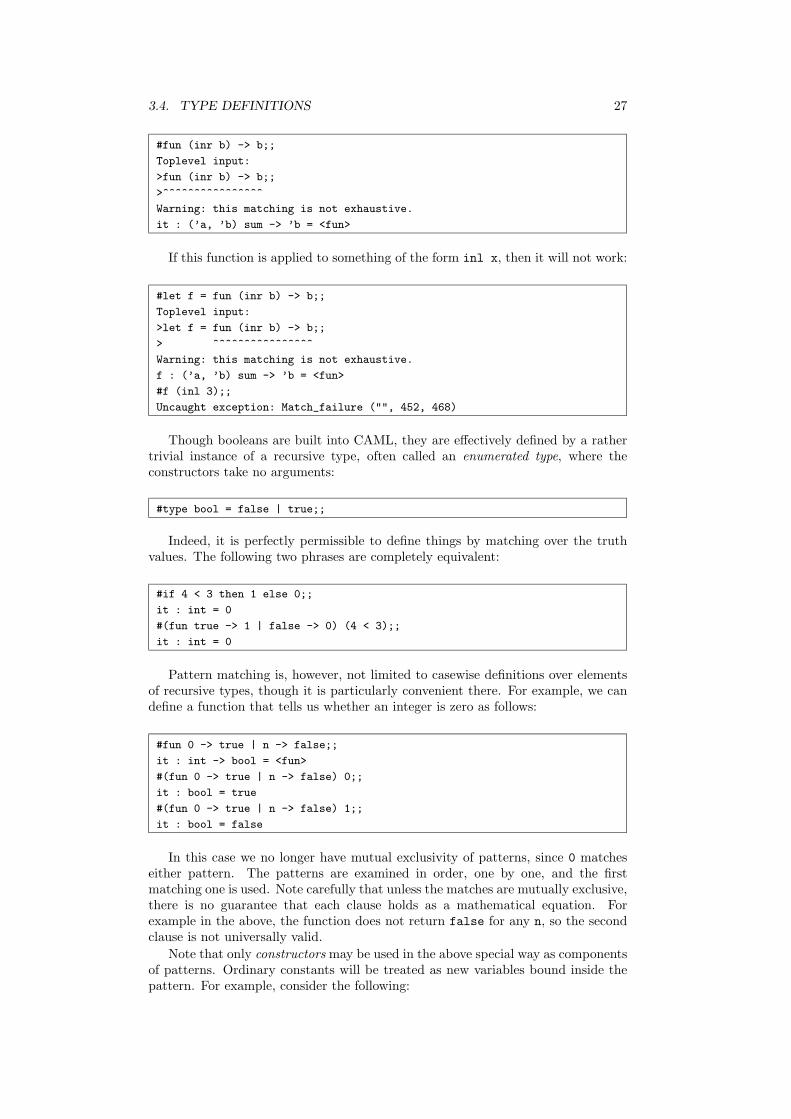
If this function is applied to something of the form inl x, then it will not work:
#let f = fun (inr b) -> b;;
Toplevel input:
>let f = fun (inr b) -> b;;
> ^^^^^^^^^^^^^^^^
Warning: this matching is not exhaustive.
f : (’a, ’b) sum -> ’b = <fun>
#f (inl 3);;
Uncaught exception: Match_failure ("", 452, 468)
Though booleans are built into CAML, they are effectively defined by a rathertrivial instance of a recursive type, often called an enumerated type, where theconstructors take no arguments:
#type bool = false | true;;
Indeed, it is perfectly permissible to define things by matching over the truthvalues. The following two phrases are completely equivalent:
#if 4 < 3 then 1 else 0;;
it : int = 0
#(fun true -> 1 | false -> 0) (4 < 3);;
it : int = 0
Pattern matching is, however, not limited to casewise definitions over elementsof recursive types, though it is particularly convenient there. For example, we candefine a function that tells us whether an integer is zero as follows:
#fun 0 -> true | n -> false;;
it : int -> bool = <fun>
#(fun 0 -> true | n -> false) 0;;
it : bool = true
#(fun 0 -> true | n -> false) 1;;
it : bool = false
In this case we no longer have mutual exclusivity of patterns, since 0 matcheseither pattern. The patterns are examined in order, one by one, and the firstmatching one is used. Note carefully that unless the matches are mutually exclusive,there is no guarantee that each clause holds as a mathematical equation. Forexample in the above, the function does not return false for any n, so the secondclause is not universally valid.
Note that only constructors may be used in the above special way as componentsof patterns. Ordinary constants will be treated as new variables bound inside thepattern. For example, consider the following:

28 CHAPTER 3. FURTHER CAML
#let true_1 = true;;
true_1 : bool = true
#let false_1 = false;;
false_1 : bool = false
#(fun true_1 -> 1 | false_1 -> 0) (4 < 3);;
Toplevel input:
>(fun true_1 -> 1 | false_1 -> 0) (4 < 3);;
> ^^^^^^^
Warning: this matching case is unused.
it : int = 1
In general, the unit element (), the truth values, the integer numerals, the stringconstants and the pairing operation (infix comma) have constructor status, as wellas other constructors from predefined recursive types. When they occur in a patternthe target value must correspond. All other identifiers match any expression and inthe process become bound.
As well as the varstructs in function expressions, there are other ways of per-forming pattern matching. Instead of creating a function via pattern matching andapplying it to an expression, one can perform pattern-matching over the expressiondirectly using the following construction:
match expression with pattern1->E1 | · · · | patternn->En
The simplest alternative of all is to use
let pattern = expression
but in this case only a single pattern is allowed.
3.4.2 Recursive types
The previous examples have all been recursive only vacuously, in that we have notdefined a type in terms of itself. For a more interesting example, we will declare atype of lists (finite ordered sequences) of elements of type ’a.
#type (’a)list = Nil | Cons of ’a * (’a)list;;
Type list defined.
Let us examine the types of the constructors:
#Nil;;
it : ’a list = Nil
#Cons;;
it : ’a * ’a list -> ’a list = <fun>
The constructor Nil, which takes no arguments, simply creates some object oftype (’a)list which is to be thought of as the empty list. The other constructorCons takes an element of type ’a and an element of the new type (’a)list andgives another, which we think of as arising from the old list by adding one elementto the front of it. For example, we can consider the following:

3.4. TYPE DEFINITIONS 29
#Nil;;
it : ’a list = Nil
#Cons(1,Nil);;
it : int list = Cons (1, Nil)
#Cons(1,Cons(2,Nil));;
it : int list = Cons (1, Cons (2, Nil))
#Cons(1,Cons(2,Cons(3,Nil)));;
it : int list = Cons (1, Cons (2, Cons (3, Nil)))
Because the constructors are distinct and injective, it is easy to see that allthese values, which we think of as lists [], [1], [1; 2] and [1; 2; 3], are distinct. Indeed,purely from these properties of the constructors, it follows that arbitrarily long listsof elements may be encoded in the new type. Actually, CAML already has a typelist just like this one defined. The only difference is syntactic: the empty list iswritten [] and the recursive constructor ::, has infix status. Thus, the above listsare actually written:
#[];;
it : ’a list = []
#1::[];;
it : int list = [1]
#1::2::[];;
it : int list = [1; 2]
#1::2::3::[];;
it : int list = [1; 2; 3]
The lists are printed in an even more natural notation, and this is also allowed forinput. Nevertheless, when the exact expression in terms of constructors is needed,it must be remembered that this is only a surface syntax. For example, we candefine functions to take the head and tail of a list, using pattern matching.
#let hd (h::t) = h;;
Toplevel input:
>let hd (h::t) = h;;
> ^^^^^^^^^^^^^
Warning: this matching is not exhaustive.
hd : ’a list -> ’a = <fun>
#let tl (h::t) = t;;
Toplevel input:
>let tl (h::t) = t;;
> ^^^^^^^^^^^^^
Warning: this matching is not exhaustive.
tl : ’a list -> ’a list = <fun>
The compiler warns us that these both fail when applied to the empty list, sincethere is no pattern to cover it (remember that the constructors are distinct). Letus see them in action:
#hd [1;2;3];;
it : int = 1
#tl [1;2;3];;
it : int list = [2; 3]
#hd [];;
Uncaught exception: Match_failure

30 CHAPTER 3. FURTHER CAML
Note that the following is not a correct definition of hd. In fact, it constrainsthe input list to have exactly two elements for matching to succeed, as can be seenby thinking of the version in terms of the constructors:
#let hd [x;y] = x;;
Toplevel input:
>let hd [x;y] = x;;
> ^^^^^^^^^^^^
Warning: this matching is not exhaustive.
hd : ’a list -> ’a = <fun>
#hd [5;6];;
it : int = 5
#hd [5;6;7];;
Uncaught exception: Match_failure
Pattern matching can be combined with recursion. For example, here is a func-tion to return the length of a list:
#let rec length =
fun [] -> 0
| (h::t) -> 1 + length t;;
length : ’a list -> int = <fun>
#length [];;
it : int = 0
#length [5;3;1];;
it : int = 3
Alternatively, this can be written in terms of our earlier ‘destructor’ functionshd and tl:
#let rec length l =
if l = [] then 0
else 1 + length(tl l);;
This latter style of function definition is more usual in many languages, notablyLISP, but the direct use of pattern matching is often more elegant.
Some other classic list functions are appending (joining together) two lists, map-ping a function over a list (i.e. applying it to each element) and reversing a list.We can define all these by recursion:

3.4. TYPE DEFINITIONS 31
#let rec append l1 l2 =
match l1 with
[] -> l2
| (h::t) -> h::(append t l2);;
append : ’a list -> ’a list -> ’a list = <fun>
#append [1;2;3] [4;5];;
it : int list = [1; 2; 3; 4; 5]
#let rec map f =
fun [] -> []
| (h::t) -> (f h)::(map f t);;
map : (’a -> ’b) -> ’a list -> ’b list = <fun>
#map (fun x -> 2 * x) [1;2;3];;
it : int list = [2; 4; 6]
#let rec rev =
fun [] -> []
| (h::t) -> append (rev t) [h];;
#rev [1;2;3;4];;
it : int list = [4; 3; 2; 1]
3.4.3 Tree structures
It is often helpful to visualize the elements of recursive types as tree structures,with the recursive constructors at the branch nodes and the other datatypes at theleaves. The recursiveness merely says that plugging subtrees together gives anothertree. In the case of lists the ‘trees’ are all rather spindly and one-sided, with thelist [1;2;3;4] being represented as:
���
@@@@@@
���
@@@
��
�@@@
��
�
1
2
3
4 []
It is not difficult to define recursive types which allow more balanced trees, e.g.
#type (’a)btree = Leaf of ’a
| Branch of (’a)btree * (’a)btree;;
In general, there can be several different recursive constructors, each with adifferent number of descendants. This gives a very natural way of representing thesyntax trees of programming (and other formal) languages. For example, here is atype to represent arithmetical expressions built up from integers by addition andmultiplication:
#type expression = Integer of int
| Sum of expression * expression
| Product of expression * expression;;
32 CHAPTER 3. FURTHER CAML
and here is a recursive function to evaluate such expressions:
#let rec eval =
fun (Integer i) -> i
| (Sum(e1,e2)) -> eval e1 + eval e2
| (Product(e1,e2)) -> eval e1 * eval e2;;
eval : expression -> int = <fun>
#eval (Product(Sum(Integer 1,Integer 2),Integer 5));;
it : int = 15
Such abstract syntax trees are a useful representation which allows all sorts ofmanipulations. Often the first step programming language compilers and relatedtools take is to translate the input text into an ‘abstract syntax tree’ according tothe parsing rules. Note that conventions such as precedences and bracketings arenot needed once we have reached the level of abstract syntax; the tree structuremakes these explicit. Recursive types similar to these are used in HOL Light todefine logical entities like terms.
3.4.4 The subtlety of recursive types
A recursive type may contain nested instances of other type constructors, includingthe function space constructor. For example, consider the following:
#type (’a)embedding = K of (’a)embedding->’a;;
Type embedding defined.
If we stop to think about the underlying semantics, this looks disquieting. Con-sider for example the special case when ’a is bool. We then have an injectivefunction K:((bool)embedding->bool)->(bool)embedding. This directly contra-dicts Cantor’s theorem that the set of all subsets of X cannot be injected into X.4
Hence we need to be more careful with the semantics of types. In fact α → βcannot be interpreted as the full function space, or recursive type constructionslike the above are inconsistent. However, since all functions we can actually createare computable, it is reasonable to restrict ourselves to computable functions only.With that restriction, a consistent semantics is possible, although the details arecomplicated.
The above definition also has interesting consequences for the type system. Forexample, we can now define a recursion operator without any explicit use of recur-sion, by using K as a kind of type cast.5 The use of let is only used for the sake ofefficiency, but we do need the extra argument z in order to prevent looping underCAML’s evaluation strategy.
#let Y h =
let g (K x) z = h (x (K x)) z in
g (K g);;
Y : ((’a -> ’b) -> ’a -> ’b) -> ’a -> ’b = <fun>
#let fact = Y (fun f n -> if n = 0 then 1 else n * f(n - 1));;
fact : int -> int = <fun>
#fact 6;;
it : int = 720
4Proof: consider C = {i(s) | s ∈ ℘(X) and i(s) 6∈ s}. If i : ℘(X) → X is injective, we havei(C) ∈ C ≡ i(C) 6∈ C, a contradiction. This is similar to the Russell paradox, and in fact probablyinspired it. The analogy is even closer if we consider the equivalent form that there is no surjectionj : X → ℘(X), and prove it by considering {s | s 6∈ j(s)}.
5Readers familiar with untyped λ-calculus may note that if the Ks are deleted, this is essentiallythe usual definition of the Y combinator.

3.4. TYPE DEFINITIONS 33
Thus, recursive types are a powerful addition to the language.

34 CHAPTER 3. FURTHER CAML

Chapter 4
Effective CAML
In this chapter, we discuss some of the techniques and tricks that CAML program-mers can use to make programs more elegant and more efficient. We then go onto discuss some additional imperative features that can be used when the purelyfunctional style seems inappropriate.
4.1 Useful combinators
The flexibility of higher order functions often means that one can write some veryuseful little functions that can be re-used for a variety of related tasks. These areoften called combinators. It often turns out that these functions are so flexible thatpractically anything can be implemented by plugging them together, rather than,say, explicitly making a recursive definition. For example, a very useful combinatorfor list operations, often called ‘itlist’ or ‘fold’, performs the following operation:
itlist f [x1; x2; . . . ;xn] b = f x1 (f x2 (f x3 (· · · (f xn b))))
A straightforward definition in CAML is:
#let rec itlist f =
fun [] b -> b
| (h::t) b -> f h (itlist f t b);;
itlist : (’a -> ’b -> ’b) -> ’a list -> ’b -> ’b = <fun>
Quite commonly, when defining a recursive function over lists, all one is doingis repeatedly applying some operator in this manner. By using itlist with theappropriate argument, one can implement such functions very easily without explicituse of recursion. A typical use is a function to add all the elements of a list ofnumbers:
#let sum l = itlist (fun x sum -> x + sum) l 0;;
sum : int list -> int = <fun>
#sum [1;2;3;4;5];;
it : int = 15
#sum [];;
it : int = 0
#sum [1;1;1;1];;
it : int = 4
Those especially keen on brevity might prefer to code sum as:
35

36 CHAPTER 4. EFFECTIVE CAML
#let sum l = itlist (prefix +) l 0;;
It is easy to modify this function to form a product rather than a sum:
#let prod l = itlist (prefix *) l 1;;
Many useful list operations can be implemented in this way. For example hereis a function to filter out only those elements of a list satisfying a predicate:
#let filter p l = itlist (fun x s -> if p x then x::s else s) l [];;
filter : (’a -> bool) -> ’a list -> ’a list = <fun>
#filter (fun x -> x mod 2 = 0) [1;6;4;9;5;7;3;2];;
it : int list = [6; 4; 2]
Here are functions to find whether either all or some of the elements of a list satisfya predicate:
#let forall p l = itlist (fun h a -> p(h) & a) l true;;
forall : (’a -> bool) -> ’a list -> bool = <fun>
#let exists p l = itlist (fun h a -> p(h) or a) l false;;
exists : (’a -> bool) -> ’a list -> bool = <fun>
#forall (fun x -> x < 3) [1;2];;
it : bool = true
#forall (fun x -> x < 3) [1;2;3];;
it : bool = false
and here are alternative versions of old favourites length, append and map:
#let length l = itlist (fun x s -> s + 1) l 0;;
length : ’a list -> int = <fun>
#let append l m = itlist (fun h t -> h::t) l m;;
append : ’a list -> ’a list -> ’a list = <fun>
#let map f l = itlist (fun x s -> (f x)::s) l [];;
map : (’a -> ’b) -> ’a list -> ’b list = <fun>
Some of these functions can themselves become useful combinators, and so onupwards. For example, if we are interested in treating lists as sets, i.e. avoidingduplicate elements, then many of the standard set operations can be expressed verysimply in terms of the combinators above:
#let mem x l = exists (fun y -> y = x) l;;
mem : ’a -> ’a list -> bool = <fun>
#let insert x l =
if mem x l then l else x::l;;
insert : ’a -> ’a list -> ’a list = <fun>
#let union l1 l2 = itlist insert l1 l2;;
union : ’a list -> ’a list -> ’a list = <fun>
#let setify l = union l [];;
setify : ’a list -> ’a list = <fun>
#let Union l = itlist union l [];;
Union : ’a list list -> ’a list = <fun>
#let intersect l1 l2 = filter (fun x -> mem x l2) l1;;
intersect : ’a list -> ’a list -> ’a list = <fun>
#let subtract l1 l2 = filter (fun x -> not mem x l2) l1;;
subtract : ’a list -> ’a list -> ’a list = <fun>
#let subset l1 l2 = forall (fun t -> mem t l2) l1;;
subset : ’a list -> ’a list -> bool = <fun>
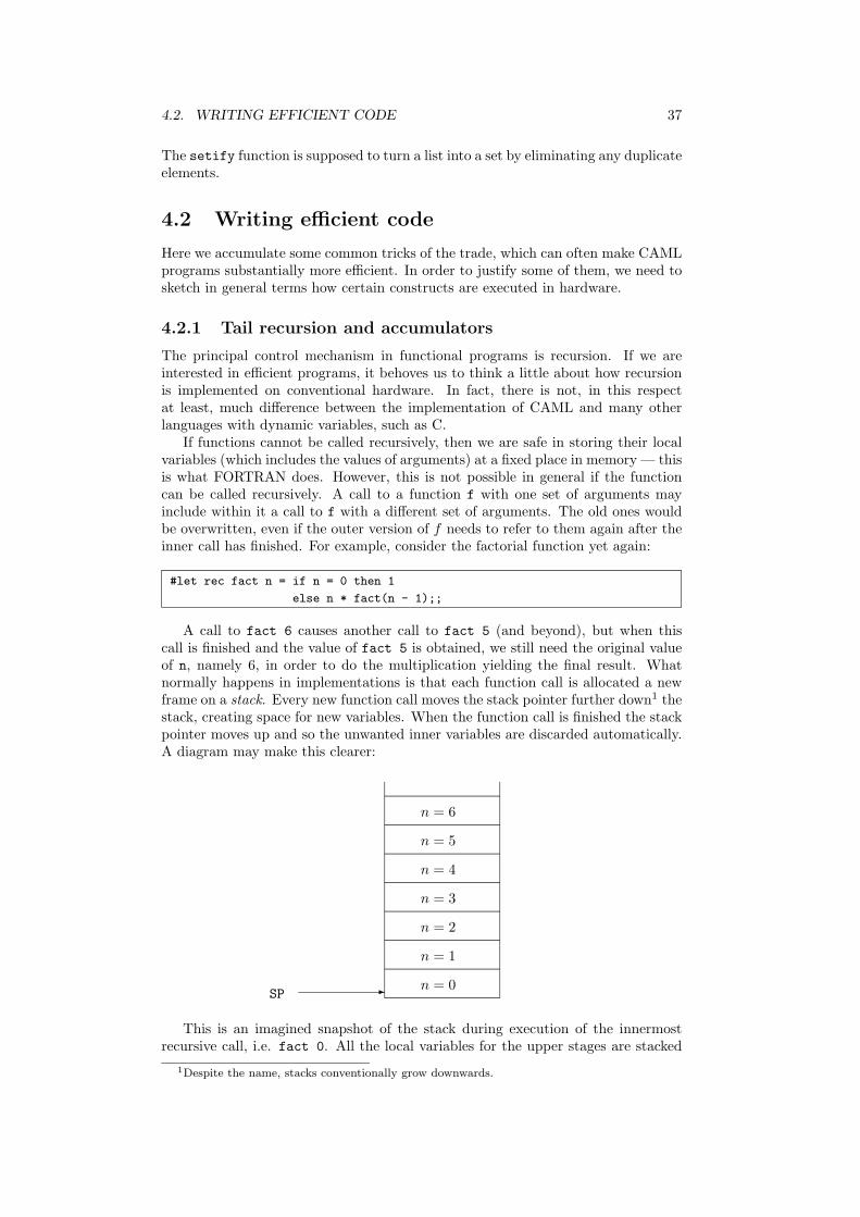
4.2. WRITING EFFICIENT CODE 37
The setify function is supposed to turn a list into a set by eliminating any duplicateelements.
4.2 Writing efficient code
Here we accumulate some common tricks of the trade, which can often make CAMLprograms substantially more efficient. In order to justify some of them, we need tosketch in general terms how certain constructs are executed in hardware.
4.2.1 Tail recursion and accumulators
The principal control mechanism in functional programs is recursion. If we areinterested in efficient programs, it behoves us to think a little about how recursionis implemented on conventional hardware. In fact, there is not, in this respectat least, much difference between the implementation of CAML and many otherlanguages with dynamic variables, such as C.
If functions cannot be called recursively, then we are safe in storing their localvariables (which includes the values of arguments) at a fixed place in memory — thisis what FORTRAN does. However, this is not possible in general if the functioncan be called recursively. A call to a function f with one set of arguments mayinclude within it a call to f with a different set of arguments. The old ones wouldbe overwritten, even if the outer version of f needs to refer to them again after theinner call has finished. For example, consider the factorial function yet again:
#let rec fact n = if n = 0 then 1
else n * fact(n - 1);;
A call to fact 6 causes another call to fact 5 (and beyond), but when thiscall is finished and the value of fact 5 is obtained, we still need the original valueof n, namely 6, in order to do the multiplication yielding the final result. Whatnormally happens in implementations is that each function call is allocated a newframe on a stack. Every new function call moves the stack pointer further down1 thestack, creating space for new variables. When the function call is finished the stackpointer moves up and so the unwanted inner variables are discarded automatically.A diagram may make this clearer:
SP - n = 0
n = 1
n = 2
n = 3
n = 4
n = 5
n = 6
This is an imagined snapshot of the stack during execution of the innermostrecursive call, i.e. fact 0. All the local variables for the upper stages are stacked
1Despite the name, stacks conventionally grow downwards.
38 CHAPTER 4. EFFECTIVE CAML
up above, with each instance of the function having its own stack frame, and whenthe calls are finished the stack pointer SP moves back up.
Therefore, our implementation of fact requires n stack frames when applied toargument n. By contrast, consider the following implementation of the factorialfunction:
#let rec tfact x n =
if n = 0 then x
else tfact (x * n) (n - 1);;
tfact : int -> int -> int = <fun>
#let fact n = tfact 1 n;;
fact : int -> int = <fun>
#fact 6;;
it : int = 720
Although tfact is also recursive, the recursive call is the whole expression; itdoes not occur as a proper subexpression of some other expression involving valuesof variables. Such a call is said to be a tail call (because it is the very last thing thecalling function does), and a function where all recursive calls are tail calls is saidto be tail recursive.
What is significant about tail calls? When making a recursive call to tfact,there is no need to preserve the old values of the local variables. Exactly thesame, fixed, area of storage can be used. This of course depends on the compiler’sbeing intelligent enough to recognize the fact, but most compilers, including CAMLLight, are. Consequently, re-coding a function so that the recursive core of it istail recursive can dramatically cut down the use of storage. For functions like thefactorial, it is hardly likely that they will be called with large enough values of n tomake the stack overflow. However the naive implementations of many list functionscan cause such an effect when the argument lists are long.
The additional argument x of the tfact function is called an accumulator, be-cause it accumulates the result as the recursive calls rack up, and is then returnedat the end. Working in this way, rather than modifying the return value on the wayback up, is a common way of making functions tail recursive.
We have remarked that a fixed area of storage can be used for the arguments toa tail recursive function. On this view, one can look at a tail recursive function asa thinly-veiled imperative implementation. There is an obvious parallel with our Cimplementation of the factorial as an iterative function:
int fact(int n){ int x = 1;
while (n > 0){ x = x * n;
n = n - 1;}return x;
}
The initialization x = 1 corresponds to our setting of x to 1 by an outer wrapperfunction fact. The central while loop corresponds to the recursive calls, the onlydifference being that the arguments to the tail recursive function make explicitthat part of the state we are interested in assigning to. Rather than assigning andlooping, we make a recursive call with the variables updated. Using similar tricksand making the state explicit, one can easily write essentially imperative code inan ostensibly functional style, with the knowledge that under standard compileroptimizations, the effect inside the machine will, in fact, be much the same.

4.2. WRITING EFFICIENT CODE 39
4.2.2 Minimizing consing
We have already considered the use of stack space. But various constructs in func-tional programs use another kind of store, usually allocated from an area called theheap. Whereas the stack grows and shrinks in a sequential manner based on theflow of control between functions, other storage used by the CAML system cannotbe reclaimed in such a simple way. Instead, the runtime system occasionally needsto check which bits of allocated memory aren’t being used any more, and reclaimthem for future use, a process known as garbage collection. A particularly importantexample is the space used by constructors for recursive types, e.g. ::. For example,when the following fragment is executed:
let l = 1::[] in tl l;;
a new block of memory, called a ‘cons cell’, is allocated to store the instance ofthe :: constructor. Typically this might be three words of storage, one being anidentifier for the constructor, and the other two being pointers to the head andtail of the list. Now in general, it is difficult to decide when this memory can bereclaimed. In the above example, we immediately select the tail of the list, so itis clear that the cons cell can be recycled immediately. But in general this can’tbe decided by looking at the program, since l might be passed to various functionsthat may or may not just look at the components of the list. Instead, one needsto analyze the memory usage dynamically and perform garbage collection of whatis no longer needed. Otherwise one would eventually run out of storage even whenonly a small amount is ever needed simultaneously.
Implementors of functional languages work hard on making garbage collectionefficient. Some claim that automatic memory allocation and garbage collectionoften works out faster than typical uses of explicit memory allocation in languageslike C (malloc etc.) While we wouldn’t go that far, it is certainly very convenientthat memory allocation is always done automatically. It avoids a lot of tedious andnotoriously error-prone parts of programming.
Many constructs beloved of functional programmers use storage that needs tobe reclaimed by garbage collection. While worrying too much about this wouldcripple the style of functional programs, there are some simple measures that canbe taken to avoid gratuitous consing (creation of cons cells). One very simple ruleof thumb is to avoid using append if possible. As can be seen by considering theway the recursive calls unroll according to the definition
#let rec append l1 l2 =
match l1 with
[] -> l2
| (h::t) -> h::(append t l2);;
this typically generates n cons cells where n is the length of the first argumentlist. There are often ways of avoiding appending, such as adding extra accumulatorarguments to functions that can be augmented by direct use of consing. A strikingexample is the list reversal function, which we coded earlier as:
#let rec rev =
fun [] -> []
| (h::t) -> append (rev t) [h];;
This typically generates about n2/2 cons cells, where n is the length of the list.The following alternative, using an accumulator, only generates n of them:

40 CHAPTER 4. EFFECTIVE CAML
#let rev =
let rec reverse acc =
fun [] -> acc
| (h::t) -> reverse (h::acc) t in
reverse [];;
Moreover, the recursive core reverse is tail recursive, so we also save stackspace, and win twice over.
For another typical situation where we can avoid appending by judicious use ofaccumulators, consider the problem of returning the fringe of a binary tree, i.e. alist of the leaves in left-to-right order. If we define the type of binary trees as:
#type btree = Leaf of string
| Branch of btree * btree;;
then a simple coding is the following
#let rec fringe =
fun (Leaf s) -> [s]
| (Branch(l,r)) -> append (fringe l) (fringe r);;
However the following more refined version performs fewer conses:
#let fringe =
let rec fr t acc =
match t with
(Leaf s) -> s::acc
| (Branch(l,r)) -> fr l (fr r acc) in
fun t -> fr t [];;
Note that we have written the accumulator as the second argument, so that therecursive call has a more natural left-to-right reading. Here is a simple example ofhow either version of fringe may be used:
#fringe (Branch(Branch(Leaf "a",Leaf "b"),
Branch(Leaf "c",Leaf "d")));;
it : string list = ["a"; "b"; "c"; "d"]
The first version creates 6 cons cells, the second only 4. On larger trees theeffect can be more dramatic. Another situation where gratuitous consing can cropup is in pattern matching. For example, consider the code fragment:
fun [] -> []
| (h::t) -> if h < 0 then t else h::t;;
The ‘else’ arm creates a cons cell even though what it constructs was in factthe argument to the function. That is, it is taking the argument apart and thenrebuilding it. One simple way of avoiding this is to recode the function as:
fun l ->
match l with
[] -> []
| (h::t) -> if h < 0 then t else l;;
However CAML offers a more flexible alternative: using the as keyword, a namemay be identified with certain components of the pattern, so that it never needs tobe rebuilt. For example:
fun [] -> []
| (h::t as l) -> if h < 0 then t else l;;

4.3. IMPERATIVE FEATURES 41
4.2.3 Forcing evaluation
We have emphasized that, since CAML does not evaluate underneath functionabstractions, one can use such constructs to delay evaluation. We will see someinteresting examples later. Conversely, however, it can happen that one wants toforce evaluation of expressions that are hidden underneath function abstractions.For example, recall the tail recursive factorial above:
#let rec tfact x n =
if n = 0 then x
else tfact (x * n) (n - 1);;
#let fact n = tfact 1 n;;
Since we never really want to use tfact directly, it seems a pity to bind it to aname. Instead, we can make it local to the factorial function:
#let fact1 n =
let rec tfact x n =
if n = 0 then x
else tfact (x * n) (n - 1) in
tfact 1 n;;
This, however, has the defect that the local recursive definition is only evaluatedafter fact1 receives its argument, since before that it is hidden under a functionabstraction. Moreover, it is then reevaluated each time fact is called. We canchange this as follows
#let fact2 =
let rec tfact x n =
if n = 0 then x
else tfact (x * n) (n - 1) in
tfact 1;;
Now the local binding is only evaluated once, at the point of declaration of fact2.According to our tests, the second version of fact is about 20% faster when calledon the argument 6. The additional evaluation doesn’t amount to much in this case,more or less just unravelling a recursive definition, yet the speedup is significant.In instances where there is a lot of computation involved in evaluating the localbinding, the difference can be spectacular. In fact, there is a sophisticated researchfield of ‘partial evaluation’ devoted to performing optimizations like this, and muchmore sophisticated ones besides, automatically. In a sense, it is a generalization ofstandard compiler optimizations for ordinary languages such as ‘constant folding’.In production ML systems, however, it is normally the responsibility of the user toforce it, as it is here in CAML Light.
We might note, in passing, that if functions are implemented by plugging to-gether combinators, with fewer explicit function abstractions, there is more chancethat as much of the expression as possible will be evaluated at declaration time. Totake a trivial example, f ◦ g will perform any evaluation of f and g that may bepossible, whereas λx. f(g x) will perform none at all until it receives its argument.On the other side of the coin, when we actually want to delay evaluation, we reallyneed lambdas, so a purely combinatory version is impossible.
4.3 Imperative features
CAML has a fairly full complement of imperative features. We will not spendmuch time on the imperative style of programming, and we assume readers already

42 CHAPTER 4. EFFECTIVE CAML
have sufficient experience. Therefore, we treat these topics fairly quickly with fewillustrative examples. However some imperative features are used in HOL Light,and some knowledge of what is available will stand the reader in good stead forwriting practical CAML code.
4.3.1 Exceptions
We have seen on occasion that certain evaluations fail, e.g. through a failure inpattern matching. There are other reasons for failure, e.g. attempts to divide byzero.
#1 / 0;;
Uncaught exception: Division_by_zero
In all these cases the compiler complains about an ‘uncaught exception’. Anexception is a kind of error indication, but it need not always be propagated to thetop level. There is a type exn of exceptions, which is effectively a recursive type,though it is usually recursive only vacuously. Unlike with ordinary types, one canadd new constructors for the type exn at any point in the program via an exceptiondeclaration, e.g.
#exception Died;;
Exception Died defined.
#exception Failed of string;;
Exception Failed defined.
While certain built-in operations generate (one usually says raise) exceptions,this can also be done explicitly using the raise construct, e.g.
#raise (Failed "I don’t know why");;
Uncaught exception: Failed "I don’t know why"
For example, we might invent our own exception to cover the case of taking thehead of an empty list:
#exception Head_of_empty;;
Exception Head_of_empty defined.
#let hd = fun [] -> raise Head_of_empty
| (h::t) -> h;;
hd : ’a list -> ’a = <fun>
#hd [];;
Uncaught exception: Head_of_empty
Normally exceptions propagate out to the top, but they can be ‘caught’ insidean outer expression by using try ...with followed by a series of patterns to matchexceptions, e.g.
#let headstring sl =
try hd sl
with Head_of_empty -> ""
| Failed s -> "Failure because "^s;;
headstring : string list -> string = <fun>
#headstring ["hi"; "there"];;
it : string = "hi"
#headstring [];;
it : string = ""

4.3. IMPERATIVE FEATURES 43
It is a matter of opinion whether exceptions are really an imperative feature.On one view, functions just return elements of a disjoint sum consisting of theirvisible return type and the type of exceptions, and all operations implicitly passback exceptions. Another view is that exceptions are a highly non-local control flowperversion, analogous to goto.2 Whatever the semantic view one takes, exceptionscan often be quite useful.
4.3.2 References and arrays
CAML does have real assignable variables, and expressions can, as a side-effect,modify the values of these variables. They are explicitly accessed via references(pointers in C parlance) and the references themselves behave more like ordinaryCAML values. Actually this approach is quite common in C too. For example, if onewants so-called ‘variable parameters’ in C, where changes to the formal parametersof a function propagate outside, the only way to do it is to pass a pointer, so that thefunction can dereference it. Similar techniques are often used where the function isto pass back composite data.
In CAML, one sets up a new assignable memory cell with the initial contents xby writing ref x. (Initialization is compulsory.) This expression yields a reference(pointer) to the cell. Subsequent access to the contents of the cell requires an explicitdereference using the ! operator, similar to unary * in C. The cell is assigned tousing a conventional-looking assignment statement. For example:
#let x = ref 1;;
x : int ref = ref 1
#!x;;
it : int = 1
#x := 2;;
it : unit = ()
#!x;;
it : int = 2
#x := !x + !x;;
it : unit = ()
#x;;
it : int ref = ref 4
#!x;;
it : int = 4
Note that in most respects ref behaves like a type constructor, so one canpattern-match against it. Thus one could actually define an indirection operatorlike !:
#let contents_of (ref x) = x;;
contents_of : ’a ref -> ’a = <fun>
#contents_of x;;
it : int = 4
As well as being mutable, references are sometimes useful for creating explicitlyshared data structures. One can easily create graph structures where numerousnodes contain a pointer to some single subgraph.
Apart from single cells, one can also use arrays in CAML. In CAML these arecalled vectors. An array of elements of type α has type α vect. A fresh vector of sizen, with each element initialized to x — once again the initialization is compulsory— is created using the following call:
2Perhaps more precisely, to C’s setjmp and longjmp.
44 CHAPTER 4. EFFECTIVE CAML
#make_vect n x;;
One can then read element m of a vector v using:
#vect_item v m;;
and write value y to element m of v using:
#vect_assign v m y;;
These operations correspond to the expressions v[m] and v[m] = y in C. Theelements of an array are numbered from zero. For example:
#let v = make_vect 5 0;;
v : int vect = [|0; 0; 0; 0; 0|]
#vect_item v 1;;
it : int = 0
#vect_assign v 1 10;;
it : unit = ()
#v;;
it : int vect = [|0; 10; 0; 0; 0|]
#vect_item v 1;;
it : int = 10
All reading and writing is constrained by bounds checking, e.g.
#vect_item v 5;;
Uncaught exception: Invalid_argument "vect_item"
4.3.3 Sequencing
There is no need for an explicit sequencing operation in CAML, since the normalrules of evaluation allow one to impose an order. For example one can do:
#let _ = x := !x + 1 in
let _ = x := !x + 1 in
let _ = x := !x + 1 in
let _ = x := !x + 1 in
();;
and the expressions are evaluated in the expected order. Here we use a specialpattern which throws away the value, but we could use a dummy variable nameinstead. Nevertheless, it is more attractive to use the conventional notation forsequencing, and this is possible in CAML by using a single semicolon:
#x := !x + 1;
x := !x + 1;
x := !x + 1;
x := !x + 1;;

4.3. IMPERATIVE FEATURES 45
4.3.4 Interaction with the type system
While polymorphism works very well for the pure functional core of CAML, it hasunfortunate interactions with some imperative features. For example, consider thefollowing:
#let l = ref [];;
Then l would seem to have polymorphic type α list ref . In accordance withthe usual rules of let-polymorphism we should be able to use it with two differenttypes, e.g. first
#l := [1];;
and then
#hd(!l) = true;;
But this isn’t reasonable, because we would actually be writing something as anobject of type int then reading it as an object of type bool. Consequently, somerestriction on the usual rule of let polymorphism is called for where references areconcerned. There have been many attempts to arrive at a sound but convenientrestriction of the ML type system, some of them very complicated. Recently, dif-ferent versions of ML seem to be converging on a relatively simple method, calledthe value restriction, due to Wright (1996), and CAML implements this restriction,with a twist regarding toplevel bindings. Indeed, the above sequence fails. But theintermediate behaviour is interesting. If we look at the first line we see:
#let l = ref [];;
l : ’_a list ref = ref []
The underscore on the type variable indicates that l is not polymorphic inthe usual sense; rather, it has a single fixed type, although that type is as yetundetermined. The second line works fine:
#l := [1];;
it : unit = ()
but if we now look at the type of l, we see that:
#l;;
it : int list ref = ref [1]
The pseudo-polymorphic type has now been fixed. Granted this, it is clear thatthe last line must fail:
#hd(!l) = true;;
Toplevel input:
>hd(!l) = true;;
> ^^^^
This expression has type bool,
but is used with type int.
So far, this seems quite reasonable, but we haven’t yet explained why the sameunderscored type variables occur in apparently quite innocent purely functionalexpressions, and why, moreover, they often disappear on eta-expansion, e.g.
46 CHAPTER 4. EFFECTIVE CAML
#let I x = x;;
I : ’a -> ’a = <fun>
#I o I;;
it : ’_a -> ’_a = <fun>
#let I2 = I o I in fun x -> I2 x;;
it : ’_a -> ’_a = <fun>
#fun x -> (I o I) x;;
it : ’a -> ’a = <fun>
Other techniques for polymorphic references often rely on encoding in the typesthe fact that an expression may involve references. This seems natural, but it canlead to the types of functions becoming cluttered with this special information. Itis unattractive that the particular implementation of the function, e.g. imperativeor functional, should be reflected in its type.
Wright’s solution, on the other hand, uses just the basic syntax of the expressionbeing let-bound, insisting that it is a so-called value before generalizing the type.What is really wanted is knowledge of whether the expression may cause side-effectswhen evaluated. However since this is undecidable in general, the simple syntacticcriterion of its being or not being a value is used. Roughly speaking, an expressionis a value if it admits no further evaluation according to the CAML rules — thisis why an expression can often be made into a value by performing a reverse etaconversion. Unfortunately this works against the techniques for forcing evaluation.
Further reading
Hints and tips for practical programming can be found in many functional program-ming books, e.g. Paulson (1991). Methods used by language implementations toperform garbage collection are discussed in depth by Jones and Lins (1996).

Part II
HOL tutorial
47


Chapter 5
Primitive basis of HOL Light
The introductory chapter gave a brief introduction to the key ideas behind HOL andsimple interaction with the system. Here we explain more systematically how math-ematical and logical assertions are represented in HOL, and list all the primitiveways of producing theorems.
We should distinguish carefully between abstract and concrete syntax. The ab-stract syntax of a term, which HOL deals with internally, is a tree-like CAML datastructure indicating how the term is built up from its components. While this isconvenient to manipulate, humans are more used to representing terms by a linearsequence of characters, the concrete syntax. HOL’s quotation parser automaticallytranslates the concrete syntax into the abstract syntax, and its prettyprinter per-forms an inverse mapping back to concrete syntax. For simple use of HOL, it is notnecessary to think much about the distinction, still less to understand details of theabstract syntax. However, we think it is best to cover this early, since it shows howsimple the underlying structures really are. The present chapter can be read as anabstract description of the HOL logic, without considering the actual implementa-tion in CAML. However when we discuss concrete syntax, we are implicitly talkingabout that accepted by HOL’s parser.
5.1 Terms
HOL’s logic is based on λ-calculus, a formalism invented by Alonzo Church. In HOL,as in λ-calculus, terms are built up starting just from constants and variables usingapplication and abstraction. All mathematical and logical assertions are representedin this uniform way.
Constants and variables are probably familiar to the reader from an informalunderstanding of mathematics. They are used as the building-blocks of terms.Variables can have any name, e.g. n, x, p. Constants, e.g. [] (the empty list), >(true) and ⊥ (false), are intended to be abbreviations for other terms, and exceptfor a couple of primitive ones such as equality itself, need to have been definedbefore they can be used in terms. We will see below how the user can define newconstants.
Application is application of a function to an argument, an operation used con-stantly in mathematics. The customary concrete syntax for the application of afunction f to an argument t is f(t). HOL, following lambda-calculus convention,allows the parentheses to be omitted, unless they are needed because t is itself acompound term. For example, f(g(x)) needs at least the outer pair of parentheses,as HOL’s parser interprets f g x to mean (f(g))(x), for reasons explained shortly.
Abstraction is in a precise sense a converse operation to application. Given
49

50 CHAPTER 5. PRIMITIVE BASIS OF HOL LIGHT
a variable x and a term t, which may or may not contain x, one can constructthe so-called lambda-abstraction λx. t, which means ‘the function of x that yieldst’. (In HOL’s ASCII concrete syntax the backslash is used, e.g. \x. t.) Forexample, λx. x+ 1 is the function that adds one to its argument. Abstractions arenot often seen in informal mathematics, but they have at least two merits. First,they allow one to write anonymous function-valued expressions without namingthem (occasionally one sees x 7→ t[x] used for this purpose), and since our logic isavowedly higher order, it’s desirable to place functions on an equal footing with first-order objects in this way. Secondly, they make variable dependencies and bindingexplicit; by contrast in informal mathematics one often writes f(x) in situationswhere one really means λx. f(x).
We should give some idea of how ordinary mathematical and logical vocabulary(like x + 1 above) is represented in this simple term structure. The basic idea isquite simple. Fixed operations that one wants to use have constants correspondingto them. For example, the negation of a real number is represented by a constant--, and so −x is represented by the application of the constant -- to the variablex. Exactly the same idea is used for logical operations like negation (‘not’), so ¬p(‘not p’) is represented by the application of the logical negation constant ~ to theterm p, whatever it may be.
Application makes no special provision for functions of more than one argument,such as addition. The trick used is known as currying, after the logician Curry(1930). (Actually the device had previously been used by both Frege (1893) andSchonfinkel (1924), but it’s easy to understand why the corresponding appellationshaven’t caught the public imagination.) The trick is to make the operation takeits arguments ‘one at a time’. For example, rather than considering addition as afunction R × R → R, consider it as a function R → (R → R). It accepts a singleargument a, and yields a new function of one argument that adds a to its argument.This intermediate function is applied to the second argument, say b, and yields thefinal result a + b. In other words, what we write as a + b is represented by HOLas (+ a)(b). (Certain operations like + are written infix in the concrete syntax, forthe sake of familiarity. But the use of currying is independent of this.)
This approach is used for many multiple-argument functions in HOL. However,there is also a pairing operation ‘,’, once again written infix in the concrete syntax,that can also be used to form pairs of terms into new terms. Of course, this itselfhas to be curried, but all other functions can be written in ‘uncurried’ form to takea tuple as its argument. Thus, what is written in the concrete syntax as f(x, y) isactually represented in HOL as f((, x)(y)).
Operations that bind variables are common in mathematics. For example, inlimx→∞
1x , the variable x is bound by a variable-binding operation lim, and serves
merely to connect different parts of the term. It can be renamed consistently, e.g.limy→∞
1y . By contrast, the inner term 1
x on its own depends on the value of x, andhere x is said to be free. Some other examples of bound variables in mathematicsand logic are the variable x in the set abstraction {x | P} (‘the set of all x such thatP ’), the variable n in ΣNn=1n (‘the sum of all n from 1 up to N ’) and the variable z in∀z. P (‘for all z, P holds’). All these variable-binding operations are represented inHOL using special constants but with the actual variable-binding implemented bylambda-abstraction. For example, there is a constant liminf (‘limit at infinity’) andone then represents limx→∞
1x by liminf(λx. 1
x ), or expanding the body completely,liminf(λx. (/ 1)(x)). This means one should think of liminf as a function fromreal functions to reals, i.e. (R → R) → R. Similarly, the logical assertion ∀x. P isrepresented using the constant ! as !(λx. P ).
It is well-known that there is a 1-1 correspondence between sets of elements(drawn from some global ‘universe’ set U), and predicates or ‘characteristic func-tions’ U → 2, where 2 is some 2-element set of truth values. In HOL, there is no

5.2. TYPES 51
separate notion of ‘set’: they are identified with predicates, i.e. Boolean-valuedfunctions. Thus, one can simply write s x instead of x ∈ s, though the latter isalso possible using the infix constant IN, e.g. x IN s. It is thus normal and oftenconvenient to slip between thinking of truth-functions as predicates or as sets, evenwithin the same term.
5.2 Types
Application and abstraction are converse in the precise sense that (λx. t)(x) isequal to t, and there is a primitive HOL rule to make this inference and producethe theorem ` (λx. t)(x) = t. More generally, HOL is capable of proving that` (λx. t)(s) = t[s/x] where the right-hand side denotes the appropriate (see later)replacement of each instance of x in t by s. For example, (λx. 1 + x)(y) = 1 + y.Unfortunately, even these banalities would allow one to get inconsistencies withoutfurther restrictions. For example, using the logical negation operation, we can derivethe Russell paradox about the set of all sets that do not contain themselves (thinkof P x as x ∈ P if preferred):
` (λx. ¬(x x))(λx. ¬(x x)) = ¬((λx. ¬(x x))(λx. ¬(x x)))
In other words, something is equal to its own logical negation! The problemseems to arise because no proper distinction of levels is made: x is treated both asa predicate and the argument to a predicate. Even if it didn’t lead to inconsistency,one might argue that it looks a bit strange. Normally one likes to have a clear idea ofwhat sort of mathematical object a term denotes — our explanation of currying, forexample, leaned on the idea that addition is thought of as a function R→ (R→ R).
Accordingly, Church (1940) augmented λ-calculus with a theory of types, simpli-fying Russell’s system from Principia Mathematica (Whitehead and Russell 1910)and giving what is often called ‘simple type theory’. HOL follows this system quiteclosely. Every term has a unique type which is either one of the basic types or theresult of applying a type constructor to other types. The only basic type in HOLis initially the type of booleans bool and the only type operator is the functionspace constructor →. (Many others are added later, as we shall see.) HOL extendsChurch’s system by allowing also ‘type variables’ which give a form of polymor-phism. Constants with polymorphic type are generic, and can have various typesresulting from fixing the names of the type variables. For example, the equalityrelation has type α → α → bool where α is a type variable. This means it can beused with any types, even if they themselves involve type variables, replacing α.
Just as in typed programming languages, functions may only be applied toarguments of the right type; only a function of type f : γ → . . . may be applied toan argument of type γ.
For familiarity, types are written in a concrete syntax with some type construc-tors like → written infix. Just as with constant and variable terms, type variablesand type constants are not distinguished syntactically: HOL’s parser assumes thateverything whose name corresponds to a constant is a constant, and every otheridentifier is a variable. However, it’s customary to use names beginning with anuppercase letter for type variables, e.g. A and State. Examples of HOL types then,include bool and A → bool (where A is a type variable). We write t : γ to indicatethat a term t has type γ. Readers familiar with set theory may like to think of typesas sets within which the objects denoted by the terms live, so t : γ can be read ast ∈ γ. Note that the use of the colon is already standard in set theory when usedfor function spaces, i.e. one typically writes f : A→ B rather than f ∈ A→ B.

52 CHAPTER 5. PRIMITIVE BASIS OF HOL LIGHT
5.3 Primitive inference rules
The HOL formal system allows the deduction of arbitrary sequents of the formφ1, . . . , φn ` ψ (read as ‘if φ1 and . . . and φn then ψ’) where the terms involvedhave type bool. (Where there are no assumptions it is customary to write just ` ψ.)There are no additional logical constants involved in the basic deductive system.The derivable sequents are those that can be generated by the following inferencerules. Each rule is written with the conclusion below a line and the hypothesesabove, and with the standard name for the inference rule, corresponding in fact toa CAML identifier in HOL, at the right.
` t = tREFL
This rule says that equality is reflexive.
Γ ` s = t ∆ ` t = uΓ ∪∆ ` s = u
TRANS
This rule says that equality is transitive. It is of course necessary to include inthe conclusion theorem any assumption that may have played a role in deducingthe top two theorems.
Γ ` s = t ∆ ` u = vΓ ∪∆ ` s(u) = t(v)
MK COMB
This says that equal functions applied to equal arguments give equal results.We have assumed without comment that the types agree, e.g. s : σ → τ , t : σ → τ ,u : σ and v : σ.
Γ ` s = tΓ ` (λx. s) = (λx. t)
ABS
This rule requires that x is not a free variable in any of the assumptions Γ. It saysthat if, without using any special properties of x, we deduced that two expressionsinvolving x are equal, then the functions that take x to those values are equal.
` (λx. t)x = tBETA
This expresses the fact that combination and abstraction are converse opera-tions, i.e. ‘the function that takes an argument x to t’, applied to an argument x,gives t.
{p} ` p ASSUME
This says simply that from any p we can deduce p. Of course, p must have typebool.
Γ ` p = q ∆ ` pΓ ∪∆ ` q EQ MP
This connects equality with deduction, saying that if p and q are equal, and wecan deduce p, then we can deduce q (from the appropriately combined assumptions).
Γ ` p ∆ ` q(Γ− {q}) ∪ (∆− {p}) ` p = q
DEDUCT ANTISYM RULE
This rule also connects equality and deduction, effectively saying that equalityon the boolean type represents logical equivalence. Ignoring extra hypotheses fora moment, it says that if we can deduce p from q and q from p, then p and q areequal, under the accumulated assumptions.

5.4. DEFINITIONS 53
Γ[x1, . . . , xn] ` p[x1, . . . , xn]Γ[t1, . . . , tn] ` p[t1, . . . , tn]
INST
This rule expresses the fact that variables are to be interpreted as schematic,i.e. if p is true for variables x1, . . . , xn, then we can replace those variables by anyterms of the same type and still get something true. Note that the substitution isalso applied to all hypotheses.
Γ[α1, . . . , αn] ` p[α1, . . . , αn]Γ[γ1, . . . , γn] ` p[γ1, . . . , γn]
INST TYPE
This is the same, but for substitution of type variables rather than term vari-ables.
5.4 Definitions
All theorems in HOL are deduced using just the above rules, starting from a smallset of axioms, which we will discuss shortly. Mathematics in HOL is derived justfrom these very basic axioms. However there is a special rule of definition, whichallows the addition of new constants and corresponding new axioms provided theyare purely definitional in character.1 If t : τ is any term without free (term or type)variables, and c : τ an unused constant, then c : τ may be added to the stock ofconstants, and the axiom ` c = t included as a theorem.
One can also define new types and type constructors in HOL. Given any subsetof a type γ, marked out by its characteristic predicate P : γ → bool, then given atheorem asserting that P is nonempty, one can define a new type δ (or type operatorif γ contains type variables) in bijection with this set.
'
&
$
%
'
&
$
%
'
&
$
%newtype
δ
existingtype
γ
�
bijections-
P
Both these definitional principles give a way of producing new mathematicaltheories without compromising soundness: one can easily prove that these principlesare consistency-preserving. Effectively, constant definitions could be avoided simplyby writing the definitional expansion out in full, while type definitions could beavoided by incorporating appropriate set constraints into theorems: rather thansaying ∀x : δ. . . . one could say ∀y : γ. P (y)⇒ . . ., with the appropriate isomorphicmappings.2
1From a logical point of view, we may say that HOL is actually an evolving sequence of logicalsystems, each a conservative extension of previous ones.
2In general, the logical core of HOL is reasonably intuitionistic, with classical principles intro-duced later as axioms. However the above definitional principle jars slightly with this since one ofthe type bijections is a total function γ → δ. This is at least weakly nonconstructive, allowing usfor example to pass from p⇒ ∃x. q[x] to ∃x. p⇒ q[x].
54 CHAPTER 5. PRIMITIVE BASIS OF HOL LIGHT
5.5 Derived rules
HOL’s logic is then built up by including constants for the usual logical operations.An attractive feature is that these do not need to be postulated: it has been knownsince Henkin (1963) how to define all logical constants in terms of equality, at leastfrom a classical point of view. We do things in an ‘intuitionistic’ manner, givinguseful deductive rules before we later assert the Law of the Excluded Middle, i.e.that every Boolean term is either true or false. While it is more typical (Prawitz1965) to take a few additional logical constants such as ∀ and ⇒ as primitive, ourapproach is very similar to the usual definitions of the internal logic of a topos; seee.g. Lambek and Scott (1986).
We will now show how all the logical constants are defined. These are > (true),∧ (and), ⇒ (implies), ∀ (for all), ∃ (there exists), ∨ (or), ⊥ (false) ¬ (not) and ∃!(there exists a unique). Recall that what we write as ∀x.P [x] is a syntactic sugaringof ∀(λx. P [x]). Using this technique, quantifiers and the Hilbert ε operator can beused as if they bound variables, but with all binding implemented in terms of λ-calculus. There are several examples in this book.
> = (λx. x) = (λx. x)∧ = λp. λq. (λf. f p q) = (λf. f > >)⇒ = λp. λq. p ∧ q = p
∀ = λP. P = λx.>∃ = λP. ∀Q. (∀x. P (x)⇒ Q)⇒ Q
∨ = λp. λq. ∀r. (p⇒ r)⇒ (q ⇒ r)⇒ r
⊥ = ∀P. P¬ = λt. t⇒ ⊥∃! = λP. ∃P ∧ ∀x. ∀y. P x ∧ P y ⇒ (x = y)
While these might look puzzling at first sight, a little thought will convincethe reader that they express what is intended. For example ∀x. P [x], or withoutsugaring ∀(λx. P [x]), says that for any a, P [a], or equivalently (λx. P [x]) a, is true.This is exactly the same as saying that λx. P [x] is a constant function that alwaysreturns > (true), which is how ∀ is defined.
From the above definitions and the primitive rules, it is then possible to definederived inference rules that give convenient ways of manipulating logical formulaswithout explicitly taking everything back to the definitions. Because HOL is aprogrammable system in the LCF style, these can all be encapsulated as CAMLfunctions that look to the user the same as primitive rules.
5.6 Classical axioms
That concludes the logic proper, and in fact quite a bit of interesting mathematics,e.g. infinitary inductive definitions, can be developed just from that basis (Harrison1995). But for general use we adopt three more axioms.
• First, there is an axiom of extensionality, which we encode as an η-conversiontheorem: ` (λx. t x) = t.
• Secondly, we introduce one new primitive logical constant ε, of polymorphictype (α→ bool)→ α, the so-called Hilbert choice operator. It is accompaniedby a new axiom giving the basic property of ε, namely that it picks outsomething satisfying P whenever there is something to pick:
5.6. CLASSICAL AXIOMS 55
` ∀x. P (x)⇒ P (εx. P (x))
The intuitive reading of εx. P (x) is ‘some x such that P (x)’, which is aninvaluable idiom when expressing some mathematical assertions. (Note thatif there isn’t anything satisfying P (x), then εx. P (x) is still well-defined, butone can’t prove any interesting properties of it.) However the above axiomisn’t just an innocent convenience: it is a form of the Axiom of (global)Choice; since P can contain other variables, one can pass from ∀x. ∃y. P [x, y]to ∀x. P [x, εy. P [x, y]]. Rather surprisingly, it also makes the logic classical,i.e. allows us to prove the theorem ` ∀p. p ∨ ¬p; see Beeson (1984) for theproof we use.
• Finally we introduce a new type ind of ‘individuals’, and add an axiom ofinfinity, asserting that the type ind is infinite. The Dedekind/Peirce definitionof ‘infinite’ is used:
` ∃f : ind→ ind. (∀x1, x2. (f(x1) = f(x2))⇒ (x1 = x2))∧¬(∀y. ∃x. y = f(x))
That is, we assert the existence of a function from the type of individuals toitself that is injective but not surjective. Such a mapping is impossible if thetype is finite, since it would entail that it can be put into 1-1 correspondencewith a proper subset of itself.
From that simple foundation, all the HOL mathematics and applications, in-cluding those described here, is developed by definitional extension.

56 CHAPTER 5. PRIMITIVE BASIS OF HOL LIGHT
Chapter 6
Implementation in CAML
The above description of HOL’s logical basics abstracted away somewhat from itsactual realization in CAML. However it has a fairly direct realization as three CAMLtypes to represent HOL types, terms and theorems. (Note the object-meta distinc-tion here: one has a CAML type of data structures representing HOL types.) TheseCAML types are all treated as abstract, with members only being created via spe-cial interface functions.1 This guards against construction of meaningless types(e.g. using undefined type constructors), ill-typed terms, and theorems that havenot been proved using the primitive rules.
6.1 Types
Each HOL type is either a type variables, or a type constructor applied to othertypes. Primitive types like bool are treated as nullary constructors, i.e. constructorswith no arguments. We will now show some of the most useful CAML functions formanipulating types.
get_type_arity :string -> int finds the arity of the appropriately-namedtype constructor. If there is no type constructor with that name, it fails. Forexample:
#get_type_arity "bool";;
it : int = 0
#get_type_arity "fun";;
it : int = 2
#get_type_arity "con";;
Uncaught exception: Failure "find"
The rest of the functions divide nicely into three groups: those for creating HOLtypes, those for breaking them apart, and those for testing their structure.
mk_vartype :string -> hol_type creates a type variable with the requestedname. This is permissible even if there is also a type constant of that name, butcan look confusing. For example:
#mk_vartype "A";;
it : hol_type = ‘:A‘
#mk_vartype "bool";;
it : hol_type = ‘:bool‘
1This could actually be enforced by the CAML system by separately compiling the modules.
57

58 CHAPTER 6. IMPLEMENTATION IN CAML
mk_type :string * hol_type list -> hol_type creates a composite type giventhe name of a type constructor and a list of component types of the right length.It fails if the name is not that of a constructor, or if the constructor’s arity doesn’tmatch the length of the list.
#mk_type("bool",[mk_vartype "A"]);;
Uncaught exception: Failure "mk_type: wrong number of arguments to bool"
#mk_type("bool",[]);;
it : hol_type = ‘:bool‘
#mk_type("fun",[it; it]);;
it : hol_type = ‘:bool->bool‘
dest_vartype :hol_type -> string reverses the effect of mk_vartype, i.e.takes a type variable and returns its name. It fails if the type isn’t a type vari-able.
#dest_vartype ‘:A‘;;
it : string = "A"
#dest_vartype ‘:bool‘;;
Uncaught exception: Failure "dest_vartype: type constructor not a variable"
#dest_vartype (mk_vartype "bool");;
it : string = "bool"
Analogously, dest_type :hol_type -> string * hol_type list reverses theeffect of mk_type, and fails if given a type variable.
#dest_type ‘:bool‘;;
it : string * hol_type list = "bool", []
#dest_type ‘:A‘;;
Uncaught exception: Failure "dest_type: type variable not a constructor"
#dest_type ‘:bool->bool‘;;
it : string * hol_type list = "fun", [‘:bool‘; ‘:bool‘]
The functions is_type :hol_type -> bool and is_vartype :hol_type -> booltest whether a HOL type is a composite type or a type variable respectively.
6.2 Terms
The CAML function get_const_type :string -> hol_type finds the type of theappropriately-named constant, or fails if there is no constant of that name. Someconstants have polymorphic type, meaning a type including type variables. Such aconstant can have any type that arises from replacing the component type variablesconsistently by other types. For example the equality constant is a curried operatorof two arguments, but the types of the arguments are arbitrary, provided they arethe same:
#get_const_type "=";;
it : hol_type = ‘:A->(A->bool)‘
In such cases, the type returned by get_const_type is a most general type, andcan be specialized by setting type variables appropriately. In general, terms featureinstances of polymorphic constants. The type of an arbitrary term can by foundusing type_of :term -> hol_type, e.g.

6.2. TERMS 59
#type_of ‘x:A‘;;
it : hol_type = ‘:A‘
#type_of ‘x = x‘;;
Warning: inventing type variables
it : hol_type = ‘:bool‘
By analogy with HOL types, the rest of the functions divide nicely into thosefor creating HOL terms, those for breaking them apart, and those for testing theirstructure.
mk_var :string * hol_type -> term creates a HOL variable with the chosenname and type.
#mk_var("x",mk_vartype "A");;
it : term = ‘x‘
#type_of it;;
it : hol_type = ‘:A‘
#mk_var("p",‘:bool‘);;
it : term = ‘p‘
mk_const :string * (hol_type * hol_type) list -> term is the analogousconstructor for HOL constants, but it’s a bit more complicated to use. The secondargument indicates not the desired type, but rather a list of settings for the typevariables in order to attain that type. For example:
#mk_const("=",[]);;
it : term = ‘(=)‘
#type_of it;;
it : hol_type = ‘:A->(A->bool)‘
#mk_const("=",[‘:bool‘,‘:A‘]);;
it : term = ‘(=)‘
#type_of it;;
it : hol_type = ‘:bool->(bool->bool)‘
There is an alternative function mk_mconst :string * hol_type -> term whichworks out the instantiations itself. However it is not part of the logical core, relyingas it does on higher-level functions to match up types. It will fail if the desired typecannot be realized:
#mk_mconst("=",‘:bool->bool->bool‘);;
it : term = ‘(=)‘
#type_of it;;
it : hol_type = ‘:bool->(bool->bool)‘
#mk_mconst("=",‘:A->B->C‘);;
Uncaught exception: Failure "mk_const: generic type cannot be instantiated"
mk_comb : term * term -> term creates an application; it is given two terms,one a function and one an argument, and tries to create the corresponding applica-tion term, failing if the types don’t match up.
#mk_comb(‘P:A->bool‘,‘x:A‘);;
it : term = ‘P x‘
#mk_comb(‘P:A->bool‘,‘x:B‘);;
Uncaught exception: Failure "mk_comb: types do not agree"
mk_abs :term * term -> term creates an abstraction term, given a variableto abstract over and the term to act as body. It fails if the first term argument isn’ta variable.
60 CHAPTER 6. IMPLEMENTATION IN CAML
#mk_abs(‘x:A‘,‘x:A‘);;
it : term = ‘\x. x‘
#mk_abs(it,it);;
Uncaught exception: Failure "mk_abs: not a variable"
There are now analogous destructor functions dest_var, dest_const, dest_comband dest_abs that act as inverses to the above. Strictly speaking dest_const is aninverse to mk_mconst, since it returns the constant name and type, not the instan-tiation list. Similarly, there are discriminator functions is_var, is_const, is_absand is_comb to test whether a term is in each class.
#dest_comb ‘~p‘;;
it : term * term = ‘(~)‘, ‘p‘
#dest_comb ‘\p. ~p‘;;
Uncaught exception: Failure "dest_comb: not a combination"
#dest_abs ‘\p. ~p‘;;
it : term * term = ‘p‘, ‘~p‘
#is_var ‘x:A‘;;
it : bool = true
#is_var ‘~p‘;;
it : bool = false
As well as the primitive syntax operations on terms, there are various derivedones, which avoid the need to reduce everything right down to the basic opera-tions above. For example, rator and rand (the names established lambda-calculusjargon) take respectively the operator and operand of an application, i.e. returnrespectively f and x when applied to a term f x. They can be implemented justby applying dest comb to get a pair of terms, then applying the CAML functionsfst or snd:
#let rator tm = fst(dest_comb tm);;
rator : term -> term = <fun>
#let rand tm = snd(dest_comb tm);;
rand : term -> term = <fun>
#rand ‘SUC 2‘;;
it : term = ‘2‘
#rator ‘1 + 2‘;;
it : term = ‘(+) 1‘
#rand ‘1 + 2‘;;
it : term = ‘2‘
There are also derived functions to create, break apart and test for equations:
#dest_eq ‘x = 1‘;;
it : term * term = ‘x‘, ‘1‘
#is_eq ‘x = y + 3‘;;
it : bool = true
#is_eq ‘x <= y + 3‘;;
it : bool = false
#is_eq ‘p = q‘;;
it : bool = true
#mk_eq(‘T‘,‘F‘);;
it : term = ‘T = F‘
Similarly, when the other constants are defined, they often have a correspondingset of functions to create, test, and destroy them. For example, mk imp creates an

6.3. THEOREMS 61
implication p ==> q, dest conj breaks apart a conjunction p /\ q, and is_disjtests if a term is a disjunction p \/ q.
6.3 Theorems
HOL theorems can be taken apart into a list of assumptions and a conclusionusing the function dest_thm :thm -> term list * term. The hypotheses andconclusion can be grabbed separately using hyp and concl. However they can onlybe created by using one of the primitive rules, making a term or type definition,or finally asserting an axiom. The last of these is only done three times for thebasic mathematical axioms, and thereafter HOL users are discouraged from addingnew axioms, as this does not maintain the guarantee of consistency. The primitiveinference rules were listed earlier, and their CAML realizations are simply CAMLfunctions returning something of type thm. For example:
#BETA ‘(\p. ~p) p‘;;
it : thm = |- (\p. ~p) p = ~p
#INST [‘q:bool‘,‘p:bool‘] it;;
it : thm = |- (\p. ~p) q = ~q
#TRANS (ASSUME ‘p:bool = q‘) (ASSUME ‘q:bool = r‘);;
it : thm = p = q, q = r |- p = r
#dest_thm it;;
it : term list * term = [‘p = q‘; ‘q = r‘], ‘p = r‘
New definitions are made using the function new definition, which takes anequational term ‘c = t’, where c is a variable. The system introduces a new con-stant called c and returns the theorem |- c = t for the new constant. For example:
#new_definition ‘true = T‘;;
it : thm = |- true = T
Later on, more convenient derived definitional principles are built on top of this— even new definition is bound to a more powerful derived function that can, forexample, accept function definitions in the form ‘f x1 ... xn = ...’.
The primitive function for performing type definitions is new_basic_type_definition.The user gives the desired name for the new type and for the bijections that mapbetween the old and new types, and finally a theorem asserting that the chosensubset of the existing type contains some object. For example, we can define a newtype single in bijection with the 1-element subset of bool containing just T. Theappropriate predicate is the function that asks of its argument x whether it is equalto t, i.e. \x. x = T:
#let th1 = BETA_CONV ‘(\x. x = T) T‘;;
th1 : thm = |- (\x. x = T) T = T = T
#let th2 = EQ_MP (SYM th1) (REFL ‘T‘);;
th2 : thm = |- (\x. x = T) T
#new_basic_type_definition "single" ("mk_single","abs_single") th2;;
it : thm * thm =
|- mk_single (abs_single a) = a,
|- (\x. x = T) r = abs_single (mk_single r) = r
Two theorems are returned as an ML pair, which together imply that the chosenbijections map 1-1 between the new type and the chosen subset of the old one.

62 CHAPTER 6. IMPLEMENTATION IN CAML
6.4 Some predefined constants
HOL has a large number of constants predefined. The most basic of these are thelogical operators whose definitions were given in passing above. Here is a tableshowing the conventional logical symbols, HOL’s ASCII approximation, and theEnglish reading. In the concrete syntax, they bind according to their order in theabove table, negation being strongest and the variable-binding operations weakest.
⊥ F Falsity> T Truth¬ ~ Not∧ /\ And∨ \/ Or⇒ ==> Implies≡ = If and only if∀ ! For all∃ ? There exists∃! ?! There exists a uniqueε @ Some . . . such thatλ \ The function taking . . . to
Readers are no doubt used to writing symbols like + rather than the word ‘plus’,but may well find these analogous logical operations less familiar. However, it’sworth spending some time getting accustomed to them, since they are needed tounderstand most HOL terms. Here are a few examples:
• T says ‘truth holds’.
• F ==> p says ‘if falsity holds, so does any p’.
• !x. x > 0 = (?y. x = y + 1) says ‘for all x, x is greater than zero if andonly if there exists a y such that x = y + 1’.
• x >= y /\ u > v ==> x + u > y + v says ‘if x is greater than or equal toy and u is greater than v, then x+ u is greater than y + v’.
• p /\ q ==> q \/ r says ‘if p and q are true, then either q or r is true’.
• ~(p = ~p) says ‘it is always false that p holds if and only if p does not hold’.
• (m * n = 0) = (m = 0) \/ (n = 0) says ‘mn is zero if and only if either mis zero or n is zero’.
• (\x. x + 1) 3 = 4 says that the function mapping any x to x + 1, whenapplied to the argument 3, is equal to 4.
• (?!x. P x) ==> !a. P(a) = (a = @x. P x) says ‘if there is a unique x sat-isfying P , then for all a, P holds of a if and only if a is equal to some canonicalx satisfying P ’.
• !P. (!n. (!m. m < n ==> P m) ==> P n) ==> !n. P n expresses the prin-ciple of complete mathematical induction, i.e. ‘for every predicate P overnumbers, if for each n, whenever P holds for each smaller m, then P holdsfor n, then for every n, P holds’.

6.4. SOME PREDEFINED CONSTANTS 63
There are also a lot of constants defined in mathematical theories. Most of theseshould look familiar, and in any case are summarized in a later chapter. However,the following is a list of some of the less obvious ones, which may help the readerfollow some of the examples below.
HOL notation Standard symbol MeaningSUC n n+ 1 Successor of n# (none) Natural map N→ R or N→ Z
--x −x Unary negation of xinv(x) x−1 Multiplicative inverse of xabs(x) |x| Absolute value of xm EXP n mn Natural m raised to natural power nx pow n xn Real x raised to natural number power nroot n x n
√x Positive nth root of x
Sum(n,d) f Σn+d−1i=n f(i) Sum of d terms f(i) starting with f(n)
x IN s x ∈ s x is a member of set sEMPTY ∅ The empty setUNIV none Universe set for a typex INSERT s {x} ∪ s Set s with element xs DELETE x s− {x} Set s without element xs UNION t s ∪ t Union of sets s and ts INTER t s ∩ t Intersection of sets s and ts DIFF t s− t Difference of sets s and tUNIONS s
⋃s Union of all members of s
INTERS s⋂s Intersection of all members of s
Formally, naturals, integers and reals are all different types, hence the use of amapping # between then. The usual arithmetic operations like + are overloaded,meaning that they are used for addition of reals, integers, and natural numbers.(The main exception is that EXP is used for natural numbers.) The next chapterexplains the translation from the usual symbols to different constants under thesurface.

64 CHAPTER 6. IMPLEMENTATION IN CAML

Chapter 7
Parsing and printing
We have already used the automatic quotation parsers quite extensively, and it’stime we looked at the relationship between the underlying representations and thesurface syntax in more detail. Many convenient constructs are representing usingsome special constants inside HOL, and the parser and printer transform such inter-nal representations into more palatable surface syntax. For example the conditionalexpression
if b then e1 else e2
is represented inside the logic using a constant COND:
CONS b e1 e2
Various other handy syntactic constructs are also dealt with in this way, e.g.abstractions over non-variables, and let-terms. For example
\(x,y,z). x + y + z
is represented by:
GABS (\f. !x y z. GEQ (f (x,y,z)) (x + y + z))
and
let x = 1 and y = 2 in x + y
is represented by:
LET (\x y. LET_END (x + y)) 1 2
Apart from special case like these, the parser-printer transformations are prettystraightforward. Identifiers may be declared infix, and given a precedence andassociativity (right or left) using parse as infix. Here are a few genuine examplesfrom the source code:
parse_as_infix("<",(12,"right"));;
parse_as_infix("+",(16,"right"));;
parse_as_infix("-",(18,"left"));;
parse_as_infix("IN",(11,"right"));;
parse_as_infix("UNION",(16,"right"));;
65
66 CHAPTER 7. PARSING AND PRINTING
7.1 Overloading
The parser and printer allow front-end symbols to be overloaded, and tries to resolveambiguities by exploiting type information. Before a symbol can be overloaded, itmust be given a most general type, and any term it maps to must have a typethat is an instance of this type. During typechecking, the overloaded symbol isgiven its most general type. If the typechecking process fixes the type sufficientlyto disambiguate, then the appropriate target is picked. Otherwise some instanceis defaulted, and typechecking repeated until all symbols have been resolved. Forexample, the addition symbol is made overloadable:
make_overloadable "+" ‘:A->A->A‘;;
Now in order to make ”+” overloaded to natural number, integer and real ad-dition, we do:
overload_interface ("+",‘(+):num->num->num‘);
overload_interface ("+",‘int_add:int->int->int‘);
overload_interface ("+",‘real_add:real->real->real‘);
Now the symbol + will map to one of three terms in the underlying represen-tation, decided according to type. The default chosen is always the most recentlydeclared version, real addition after the above sequence. If the user wants to avoidany defaults, then type information sometimes needs to be supplied. All the follow-ing are unambiguous:
#‘x + 1‘;;
it : term = ‘x + 1‘
#‘x:int + y‘;;
it : term = ‘x‘
#‘(x + y):real‘;;
it : term = ‘x + y‘
Instead of mapping a symbol to multiple targets, one can always choose just one.The function override interface is similar to overload interface, except thatit removes any existing mappings for the symbol first. For example, the user whodislikes the use of equality to mean logical equivalence could remap HOL Light’sinterface as follows:
#parse_as_infix("<=>",(2,"right"));;
it : unit = ()
#override_interface ("<=>",‘(=):bool->bool->bool‘);;
it : unit = ()
#‘x = F‘;;
it : term = ‘x <=> F‘
#‘x <=> F‘;;
it : term = ‘x <=> F‘
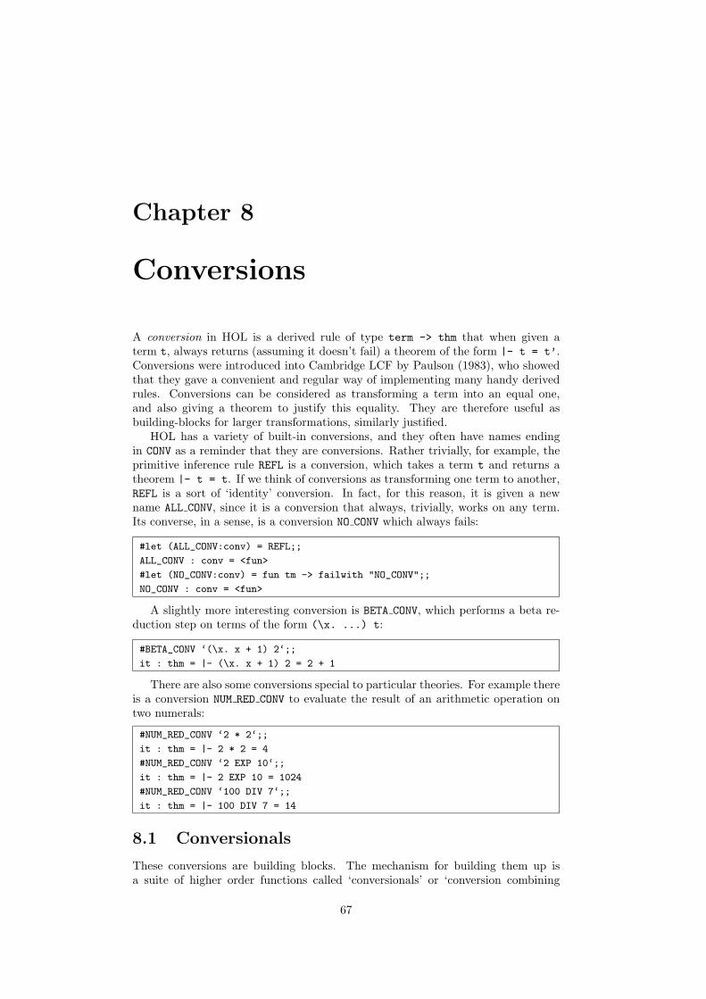
Chapter 8
Conversions
A conversion in HOL is a derived rule of type term -> thm that when given aterm t, always returns (assuming it doesn’t fail) a theorem of the form |- t = t’.Conversions were introduced into Cambridge LCF by Paulson (1983), who showedthat they gave a convenient and regular way of implementing many handy derivedrules. Conversions can be considered as transforming a term into an equal one,and also giving a theorem to justify this equality. They are therefore useful asbuilding-blocks for larger transformations, similarly justified.
HOL has a variety of built-in conversions, and they often have names endingin CONV as a reminder that they are conversions. Rather trivially, for example, theprimitive inference rule REFL is a conversion, which takes a term t and returns atheorem |- t = t. If we think of conversions as transforming one term to another,REFL is a sort of ‘identity’ conversion. In fact, for this reason, it is given a newname ALL CONV, since it is a conversion that always, trivially, works on any term.Its converse, in a sense, is a conversion NO CONV which always fails:
#let (ALL_CONV:conv) = REFL;;
ALL_CONV : conv = <fun>
#let (NO_CONV:conv) = fun tm -> failwith "NO_CONV";;
NO_CONV : conv = <fun>
A slightly more interesting conversion is BETA CONV, which performs a beta re-duction step on terms of the form (\x. ...) t:
#BETA_CONV ‘(\x. x + 1) 2‘;;
it : thm = |- (\x. x + 1) 2 = 2 + 1
There are also some conversions special to particular theories. For example thereis a conversion NUM RED CONV to evaluate the result of an arithmetic operation ontwo numerals:
#NUM_RED_CONV ‘2 * 2‘;;
it : thm = |- 2 * 2 = 4
#NUM_RED_CONV ‘2 EXP 10‘;;
it : thm = |- 2 EXP 10 = 1024
#NUM_RED_CONV ‘100 DIV 7‘;;
it : thm = |- 100 DIV 7 = 14
8.1 Conversionals
These conversions are building blocks. The mechanism for building them up isa suite of higher order functions called ‘conversionals’ or ‘conversion combining
67

68 CHAPTER 8. CONVERSIONS
operators’. These allow one to construct composite conversions in a user-definedway. For example, the conversional THENC, used infix, uses one conversion and thenafterwards, another, e.g.
#(BETA_CONV THENC NUM_RED_CONV) ‘(\x. x + 1) 2‘;;
it : thm = |- (\x. x + 1) 2 = 3
The conversional REPEATC allows one to use a conversion repeatedly until it fails(maybe zero times), e.g.
#REPEATC BETA_CONV ‘23‘;;
it : thm = |- 23 = 23
#REPEATC BETA_CONV ‘(\x. x + 1)‘;;
it : thm = |- (\x. x + 1) = (\x. x + 1)
#REPEATC BETA_CONV ‘(\x. x + 1) 2‘;;
it : thm = |- (\x. x + 1) 2 = 2 + 1
#REPEATC BETA_CONV ‘(\x. (\y. x + y) 2) 1‘;;
it : thm = |- (\x. (\y. x + y) 2) 1 = 1 + 2
8.2 Depth conversions
The conversions above are still only applied at the top level of a term. For example,the following fails because the beta-redex is deeper inside the term than expected:
#BETA_CONV ‘1 + (\x. x + 1) 2‘;;
Uncaught exception: Failure "BETA_CONV: Not a beta-redex"
However there is an additional set of conversionals that apply the given conver-sion at depth inside the term. For example ONCE DEPTH CONV applies a conversionto the first applicable term(s) encountered in a top-down traversal of the term. Nodeeper terms are examined, but several terms can be converted provided they aredisjoint:
#ONCE_DEPTH_CONV NUM_RED_CONV ‘1 + (2 + 3)‘;;
it : thm = |- 1 + 2 + 3 = 1 + 5
#ONCE_DEPTH_CONV NUM_RED_CONV ‘(1 + 1) * (1 + 1)‘;;
it : thm = |- (1 + 1) * (1 + 1) = 2 * 2
Conversions like NUM RED CONV can be used to reduce a term completely by ap-plying it in a single bottom-up sweep. This is done by the conversional DEPTH CONV,e.g.
#DEPTH_CONV NUM_RED_CONV ‘7 * (3 EXP 10) + 11‘;;
it : thm = |- 7 * 3 EXP 10 + 11 = 413354
However, this isn’t always what’s needed; sometimes the act of applying aconversion at one level can create new applicable terms lower down; in this caseDEPTH CONV will not reexamine them. Two other conversionals, TOP DEPTH CONVand REDEPTH CONV, will keep applying conversions as long as possible all over theterm.
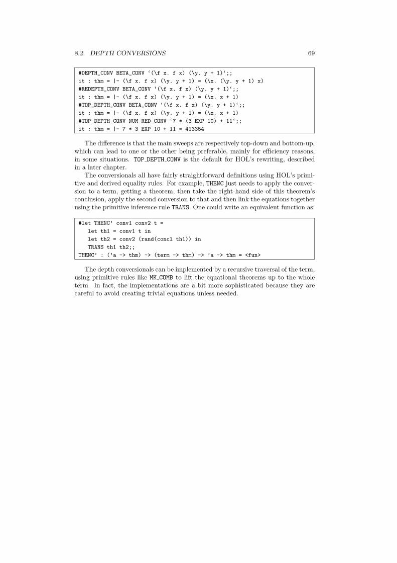
8.2. DEPTH CONVERSIONS 69
#DEPTH_CONV BETA_CONV ‘(\f x. f x) (\y. y + 1)‘;;
it : thm = |- (\f x. f x) (\y. y + 1) = (\x. (\y. y + 1) x)
#REDEPTH_CONV BETA_CONV ‘(\f x. f x) (\y. y + 1)‘;;
it : thm = |- (\f x. f x) (\y. y + 1) = (\x. x + 1)
#TOP_DEPTH_CONV BETA_CONV ‘(\f x. f x) (\y. y + 1)‘;;
it : thm = |- (\f x. f x) (\y. y + 1) = (\x. x + 1)
#TOP_DEPTH_CONV NUM_RED_CONV ‘7 * (3 EXP 10) + 11‘;;
it : thm = |- 7 * 3 EXP 10 + 11 = 413354
The difference is that the main sweeps are respectively top-down and bottom-up,which can lead to one or the other being preferable, mainly for efficiency reasons,in some situations. TOP DEPTH CONV is the default for HOL’s rewriting, describedin a later chapter.
The conversionals all have fairly straightforward definitions using HOL’s primi-tive and derived equality rules. For example, THENC just needs to apply the conver-sion to a term, getting a theorem, then take the right-hand side of this theorem’sconclusion, apply the second conversion to that and then link the equations togetherusing the primitive inference rule TRANS. One could write an equivalent function as:
#let THENC’ conv1 conv2 t =
let th1 = conv1 t in
let th2 = conv2 (rand(concl th1)) in
TRANS th1 th2;;
THENC’ : (’a -> thm) -> (term -> thm) -> ’a -> thm = <fun>
The depth conversionals can be implemented by a recursive traversal of the term,using primitive rules like MK COMB to lift the equational theorems up to the wholeterm. In fact, the implementations are a bit more sophisticated because they arecareful to avoid creating trivial equations unless needed.

70 CHAPTER 8. CONVERSIONS

Chapter 9
Derived rules
HOL has a variety of other derived rules that are not conversions, or at least aren’tused much as in the previous chapter. Here we cover some of the most basic ones.
9.1 Logical rules
All the logical constants are defined; we have seen the definitions above. From thedefinitions, rules for manipulating them directly are derived, so for most purposesusers can forget that they aren’t primitives. Most of the rules are so-called intro-duction and elimination rules of natural deduction (Prawitz 1965).1 For example,the introduction rule for conjunctions, CONJ, takes two theorems and gives a newtheorem that results from conjoining (‘anding’) them, e.g.
#CONJ (REFL ‘1‘) (ASSUME ‘x = 2‘);;
it : thm = x = 2 |- (1 = 1) /\ (x = 2)
Conversely, the elimination rules CONJUNCT1 and CONJUNCT2 take a theoremwith a conjunction as conclusion, and give new theorems for the left and rightarms. CONJ PAIR gives a pair of both, while CONJUNCTS repeatedly breaks down aconjunctive theorem into a list of theorems.
#let th1 = CONJ (REFL ‘T‘) (ASSUME ‘p /\ q‘);;
th1 : thm = p /\ q |- (T = T) /\ p /\ q
#let th2 = CONJ (REFL ‘1‘) th1;;
th2 : thm = p /\ q |- (1 = 1) /\ (T = T) /\ p /\ q
#CONJ_PAIR th2;;
it : thm * thm = p /\ q |- 1 = 1, p /\ q |- (T = T) /\ p /\ q
#CONJUNCTS th2;;
it : thm list = [p /\ q |- 1 = 1; p /\ q |- T = T; p /\ q |- p; p /\ q |- q]
#CONJUNCT2 th1;;
it : thm = p /\ q |- p /\ q
Abstracting away a bit from the implementation in CAML, we can representthe rules in the usual form as:
Γ ` p ∆ ` qΓ ∪∆ ` p ∧ q CONJ
1Although HOL uses a sequent presentation, the conventional derived rules are natural deduc-tion rules, i.e. introduction and elimination on the right, rather than left and right introduction.
71

72 CHAPTER 9. DERIVED RULES
Γ ` p ∧ qΓ ` p CONJUNCT1
Γ ` p ∧ qΓ ` q CONJUNCT2
All the other defined constants come equipped with a similar suite of rules. Inmost cases the reader will be able to guess how the corresponding CAML functionis used, and can experiment a little on the lines of the above examples.
Γ ` pΓ ` p = > EQT INTRO
Γ ` p = >Γ ` p EQT ELIM
Γ ` p⇒ q ∆ ` pΓ ∪∆⇒ q
MP
Γ ` qΓ− {p} ` p⇒ q
DISCH
Γ ` p⇒ q
Γ ∪ {p} ` q UNDISCH
Γ ` ∀x. pΓ ` p[t/x]
SPEC
Here p[t/x] denotes the result of substituting t for all free instances of x inp. HOL automatically renames variables to avoid capture if necessary, by addingprime characters. (This happens in the primitive function INST that is used in theimplementation.)
#let th1 = ASSUME ‘!x. x >= 0‘;;
th1 : thm = !x. x >= 0 |- !x. x >= 0
#let th2 = SPEC ‘y + 1‘ th1;;
th2 : thm = !x. x >= 0 |- y + 1 >= 0
#let th3 = ASSUME ‘!x. ?y. y > x‘;;
th3 : thm = !x. ?y. y > x |- !x. ?y. y > x
#let th4 = SPEC ‘y:num‘ th3;;
th4 : thm = !x. ?y. y > x |- ?y’. y’ > y
Note that the naive result of substituting would be the incorrect ?y. y > y.
Γ ` pΓ ` ∀x. p GEN
This rule will fail if the variable x is free in the assumptions Γ. Again, thisrestriction arises naturally out of one in the underlying primitives, in this case inABS.

9.1. LOGICAL RULES 73
#let th1 = REFL ‘x:num‘;;
th1 : thm = |- x = x
#let th2 = GEN ‘x:num‘ th1;;
th2 : thm = |- !x. x = x
#let th3 = GEN ‘y:num‘ th2;;
th3 : thm = |- !y x. x = x
#let th4 = ASSUME ‘x = 2‘;;
th4 : thm = x = 2 |- x = 2
#let th5 = GEN ‘x:num‘ th4;;
Uncaught exception: Failure "GEN"
#let th5 = GEN ‘y:num‘ th4;;
th5 : thm = x = 2 |- !y. x = 2
Γ ` p[t/x]Γ ` ∃x. p EXISTS
The ML invocations for this rule are relatively complicated; the function requiresthe user to specify the desired form of the result and the term t to choose. It couldwork out the latter for itself, but in general one can derive many existential theoremsfrom the same starting point, e.g.
#let th1 = REFL ‘1‘;;
th1 : thm = |- 1 = 1
#let th2 = EXISTS(‘?x. x = 1‘,‘1‘) th1;;
th2 : thm = |- ?x. x = 1
#let th3 = EXISTS(‘?x:num. x = x‘,‘1‘) th1;;
th3 : thm = |- ?x. x = x
#let th4 = EXISTS(‘?x:num. 1 = 1‘,‘23‘) th1;;
th4 : thm = |- ?x. 1 = 1
Γ ` qΓ− {p} ` (∃x. p)⇒ q
CHOOSE
This rule requires that x is not free in q nor in any of the Γ besides p.
Γ ` pΓ ` p ∨ q DISJ1
Γ ` qΓ ` p ∨ q DISJ2
Γ ` r Γ′ ` r ∆ ` p ∨ q(Γ− {p}) ∪ (Γ′ − {q}) ∪∆ ` r DISJ CASES
Γ ` ¬pΓ ` p⇒ ⊥ NOT ELIM
Γ ` p⇒ ⊥Γ ` ¬p NOT INTRO
Γ ` p ≡ ⊥Γ ` ¬p EQF ELIM
Γ ` ¬pΓ ` p ≡ ⊥ EQF INTRO

74 CHAPTER 9. DERIVED RULES
9.2 Rewriting and simplification
HOL has various rules and conversions at a somewhat higher level. Some of themost useful of these automatically work out how to instantiate variables to apply tothe case in hand. For example, the above ‘Modus Ponens’ rule requires the theoremsto match up exactly:2
#MP (ASSUME ‘x < 1 ==> x <= 1‘) (ASSUME ‘x < 1‘);;
it : thm = x > 1 ==> x >= 1, x >= 1 |- x > 1
#MP (ASSUME ‘y < 1 ==> y <= 1‘) (ASSUME ‘x < 1‘);;
Uncaught exception: Failure "MP: theorems do not agree"
A more powerful rule, MATCH MP, tries to work out settings for free or universallyquantified variables in the first theorem in order to make things match up. we canillustrate this using a built-in theorem LT IMP LE:
#let th1 = LT_IMP_LE;;
th1 : thm = |- !m n. m < n ==> m <= n
#MATCH_MP th1 (ASSUME ‘x < 1‘);;
it : thm = x < 1 |- x <= 1
A similar rule, actually a conversion, is REWR CONV. It takes an equation, perhapsuniversally quantified, and sets the variables if possible so that the left-hand sidematches the proffered term, ‘rewriting’ it. Again, we will illustrate it using a built-intheorem:
#let th1 = NOT_LE;;
th1 : thm = |- !m n. ~(m <= n) = n < m
#REWR_CONV th1 ‘~(x + 1 <= x)‘;;
it : thm = |- ~(x + 1 <= x) = x < x + 1
Since it is a conversion, REWR CONV can be combined with various depth con-versions to rewrite repeatedly at various levels of a term. Built-in functions likeREWRITE CONV take a whole list of theorems, extract rewrites from them and re-peatedly apply them to a term.3 Moreover, they throw in a set of handy rewrites toget rid of trivial propositional clutter, e.g. reducing p /\ p to p. They are one ofthe workhorses in typical HOL proofs. If the additional propositional simplificationsare not required, prefix the name with PURE:
#PURE_REWRITE_CONV[NOT_LE; LT_REFL] ‘~(x < x) \/ q‘;;
it : thm = |- ~(x < x) \/ q = ~F \/ q
#REWRITE_CONV[NOT_LE; LT_REFL] ‘~(x < x) \/ q‘;;
it : thm = |- ~(x < x) \/ q = T
As in this example, one often rewrites Boolean terms. In cases where conversionsare applied to Boolean terms, it’s often handy to convert conversions to forwardinference rules. This is done using CONV RULE, whose definition is simply:
#let CONV_RULE conv th =
EQ_MP (conv(concl th)) th;;
CONV_RULE : (term -> thm) -> thm -> thm = <fun>
#CONV_RULE(REWRITE_CONV[NOT_LE; LT_REFL]) (ASSUME ‘~(x < x) \/ q‘);;
it : thm = ~(x < x) \/ q |- T
2Actually, only up to alpha-equivalence, i.e. renaming of bound variables.3They do work by applying REWR CONV at depth, but are optimized using term nets to avoid too
many wasteful attempts to match theorems against subterms.

9.3. ORDERED REWRITING 75
Some conversions are made into rules and given names, because they are usedso often. For example:
#let BETA_RULE = CONV_RULE(REDEPTH_CONV BETA_CONV);;
BETA_RULE : thm -> thm = <fun>
#let REWRITE_RULE thl = CONV_RULE(REWRITE_CONV thl);;
REWRITE_RULE : thm list -> thm -> thm = <fun>
Still more powerful than rewriting is simplification. This allows the use of equa-tions that are conditional, i.e. of the form ` p ⇒ l = r. After matching up lwith the term if possible, setting the theorem to ` p′ ⇒ l′ = r′ the conversion isrecursively applied to the hypothesis p′, trying to reduce it to > and so eliminateit. This can often avoid tedious chains of straightforward logical reasoning. Forexample, in
#DIV_LT;;
it : thm = |- !m n. m < n ==> (m DIV n = 0)
#SIMP_CONV[DIV_LT; ARITH] ‘3 DIV 7 = 0‘;;
it : thm = |- (3 DIV 7 = 0) = T
the built-in theorem DIV LT is used as a rewrite, giving a hypothesis 3 < 7 whichis then attacked by more simplification, this time using a set of rewrites to dobasic arithmetic (described later). Simplification also accumulates context, so whentraversing a term p ⇒ q and descending to q, additional rewrites are derived fromp, e.g.
#SIMP_CONV [] ‘p /\ q ==> p‘;;
it : thm = |- p /\ q ==> p = T
The rewrite p = T is extracted from the context p and this is used to rewritethe consequent to T. The final result follows from an additional rewrite with thebuilt-in simplification p ==> T = T.
9.3 Ordered rewriting
It is possible for rewriting and simplification to go into an infinite loop, e.g. applyingtwo successive rewrites ` s = t and ` t = s alternately. However, HOL tries to avoidlooping in some cases, ignoring rewrites that would loop:
#REWRITE_CONV[ASSUME ‘x = x + 1‘] ‘x:num‘;;
Warning: discarding looping rewrite
it : thm = |- x = x
Some rewrites are said to be permutative, meaning that the left hand side canbe matched to the right hand side and vice versa. For example, there is a built-intheorem ADD SYM asserting that addition of natural numbers is commutative, andseveral others:
#ADD_SYM;;
it : thm = |- !m n. m + n = n + m
#CONJ_SYM;;
it : thm = |- !t1 t2. t1 /\ t2 = t2 /\ t1
#INSERT_COMM;;
it : thm = |- !x y s. x INSERT y INSERT s = y INSERT x INSERT s

76 CHAPTER 9. DERIVED RULES
The HOL Light approach to permutative rewrite rules has long been used inthe Boyer-Moore theorem prover, and more recently in Isabelle thanks to TobiasNipkow. They are only applied if, after instantiation, the left-hand side is “larger”than the right according to some well-founded ordering. The basic building block isORDERED_REWR_CONV. This calls REWR_CONV, but will then force failure unless in theresulting theorem Γ ` s′ = t′ one has t′ > s′ according to the given ordering > onterms. In this way, one can rewrite freely with a theorem such as ` x + y = y + xwithout fear of infinite looping.
However in conjunction with other rewrites, infinite looping can reappear. Forexample, rewriting with the above commutative law and the associative law ` (x+y) + z = x+ (y + z) one could still have an infinite rewrite:
x+ (y + z) −→ (y + z) + x
−→ y + (z + x)−→ (z + x) + y
−→ z + (x+ y)−→ (x+ y) + z
−→ x+ (y + z)
This, however, can be prevented by a suitable choice of ordering. In fact, giventhe right ordering, the associative and commutative laws together not only alwaysterminate, but actually reduce AC combinations to their canonical form. Martinand Nipkow (1990) give a slightly tricky ordering that makes the associative andcommutative laws alone give a normalizer. However a more obvious approach is toadd a third theorem, easily derived from the other two: ` x+ (y+ z) = y+ (x+ z).Now, suppose that the ordering has the following properties for any terms x, y andz:
(x+ y) + z > x+ (y + z)x+ y > y + x iff x > y
x+ (y + z) > y + (x+ z) iff x > y
Such an ordering, if it is also monotonic (if s > t then u[s] > u[t]) and total andis wellfounded on ground terms, is said to be AC-compatible. Intuitively it is clearthat ordered rewriting with these theorems will canonicalize AC combinations by‘bubbling’ terms in iterated additions to their proper place. Theorems in this classfor some associative and commutative operators are built into HOL, e.g.
#ADD_AC;;
it : thm =
|- (m + n = n + m) /\ ((m + n) + p = m + n + p) /\ (m + n + p = n + m + p)
#MULT_AC;;
it : thm =
|- (m * n = n * m) /\ ((m * n) * p = m * n * p) /\ (m * n * p = n * m * p)
#REWRITE_CONV[ADD_AC; MULT_AC] ‘x * y + z * x + w * x + x * w =
x * w + x * z + y * x + x * w‘;;
it : thm =
|- (x * y + z * x + w * x + x * w = x * w + x * z + y * x + x * w) = T
Martin and Nipkow (1990) show that one can also add laws of left and rightdistributivity for + and ∗, as well as idempotence laws ` x+x = x and ` x+(x+y) =x+y and get canonicalizers under these laws too. (For example, if + is conjunctionor disjunction.)

9.4. HIGHER ORDER MATCHING 77
#CONJ_ACI;;
it : thm =
|- (p /\ q = q /\ p) /\
((p /\ q) /\ r = p /\ q /\ r) /\
(p /\ q /\ r = q /\ p /\ r) /\
(p /\ p = p) /\
(p /\ p /\ q = p /\ q)
#REWRITE_CONV[CONJ_ACI] ‘p /\ q /\ p /\ r /\ q = r /\ q /\ p‘;;
it : thm = |- (p /\ q /\ p /\ r /\ q = r /\ q /\ p) = T
9.4 Higher order matching
HOL Light supports a limited form of higher order matching. This is immenselyuseful in order to express more general term transformations as rewrite rules. Ifonly simple ‘first order’ matching is used, the scope of rewriting, matching modusponens etc. is rather restricted. Even quite simple schematic theorems need to beinstantiated manually — a very tedious task. For example, if we want to use thetheorem:
#SKOLEM_THM;;
it : thm = |- !P. (!x. ?y. P x y) = (?y. !x. P x (y x))
to rewrite the term !n. ?m. m EXP 2 <= n /\ n < (SUC m) EXP 2, then simplerewriting won’t work; one first needs to instantiate the theorem with
P = (\n m. m EXP 2 <= n /\ n < (SUC m) EXP 2)
then beta-reduce it, and only then rewrite with it. HOL Light will do this automat-ically in some situations. For example, it will perform the following rewrite, eventhough the term isn’t literally an instance of the theorem’s left hand side:
#NOT_FORALL_THM;;
it : thm = |- !P. ~(!x. P x) = (?x. ~P x)
#REWR_CONV NOT_FORALL_THM ‘~(!n. n < n - 1)‘;;
it : thm = |- ~(!n. n < n - 1) = (?n. ~(n < n - 1))
The implementation of higher order matching aims to make matching as gen-eral as possible while keeping it deterministic. It allows higher order matches ofP x1 · · ·xn where P is an instantiable variable, but only if it can decide with cer-tainty how to instantiate the xi. Generally speaking, there are lots of possiblehigher order matches; for example the pattern P (x + y) can be matched against(a+ b) + (c+ d) in several different ways, e.g. x = a+ b, y = c+ d or x = a, y = b.In order to make the matches determinate, information is taken from correspondingvariable bindings. For example there is no doubt about the matching of ∀x. Pxto ∀n. n < n + 1, whereas with the bound variables removed one could have var-ious alternatives, e.g. P = λx. n < x + 1 and x = n. Our allowable patternscorrespond quite closely to higher order patterns, for which Miller (1991) provedeven the unification (two-way matching) problem to be decidable and deterministic(‘unitary’). We generalize higher order patterns in two ways. First, one need notsimply have variables in the patterns, but can have arbitrary terms involving onlythese ‘resolvable’ variables. Thus one can match:
|- (!x. P(SUC x)) = !x. 0 < x ==> P x
with a term:
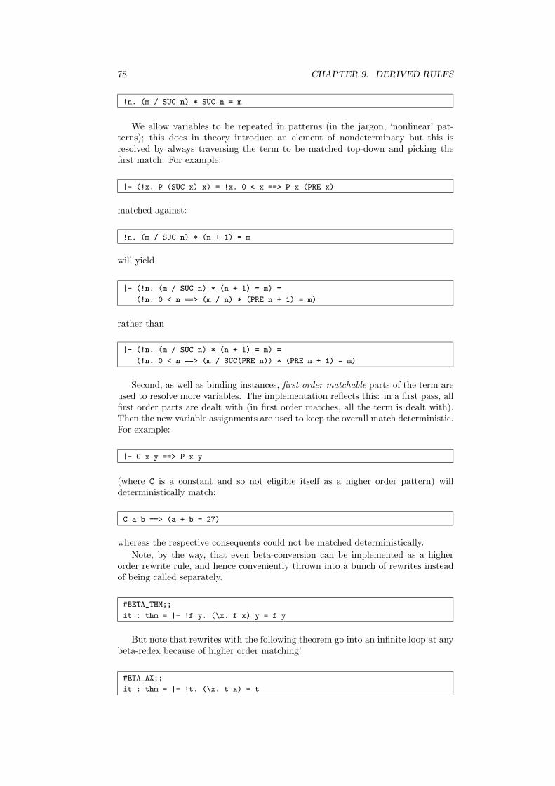
78 CHAPTER 9. DERIVED RULES
!n. (m / SUC n) * SUC n = m
We allow variables to be repeated in patterns (in the jargon, ‘nonlinear’ pat-terns); this does in theory introduce an element of nondeterminacy but this isresolved by always traversing the term to be matched top-down and picking thefirst match. For example:
|- (!x. P (SUC x) x) = !x. 0 < x ==> P x (PRE x)
matched against:
!n. (m / SUC n) * (n + 1) = m
will yield
|- (!n. (m / SUC n) * (n + 1) = m) =
(!n. 0 < n ==> (m / n) * (PRE n + 1) = m)
rather than
|- (!n. (m / SUC n) * (n + 1) = m) =
(!n. 0 < n ==> (m / SUC(PRE n)) * (PRE n + 1) = m)
Second, as well as binding instances, first-order matchable parts of the term areused to resolve more variables. The implementation reflects this: in a first pass, allfirst order parts are dealt with (in first order matches, all the term is dealt with).Then the new variable assignments are used to keep the overall match deterministic.For example:
|- C x y ==> P x y
(where C is a constant and so not eligible itself as a higher order pattern) willdeterministically match:
C a b ==> (a + b = 27)
whereas the respective consequents could not be matched deterministically.Note, by the way, that even beta-conversion can be implemented as a higher
order rewrite rule, and hence conveniently thrown into a bunch of rewrites insteadof being called separately.
#BETA_THM;;
it : thm = |- !f y. (\x. f x) y = f y
But note that rewrites with the following theorem go into an infinite loop at anybeta-redex because of higher order matching!
#ETA_AX;;
it : thm = |- !t. (\x. t x) = t

9.5. OTHER RULES 79
9.5 Other rules
As well as these handy general-purpose rules, there are some special ones for par-ticular theories, described later. For example, ARITH RULE is useful for disposing oftrivial facts of linear arithmetic over the natural numbers:
#ARITH_RULE ‘x < y ==> 4 * x + 3 < 4 * y‘;;
it : thm = |- x < y ==> 4 * x + 3 < 4 * y
Another easy rule, TAUT, proves propositional tautologies automatically, e.g.
#TAUT ‘p /\ q ==> p‘;;
it : thm = |- p /\ q ==> p
#TAUT ‘(p ==> q) \/ (q ==> p)‘;;
it : thm = |- (p ==> q) \/ (q ==> p)

80 CHAPTER 9. DERIVED RULES
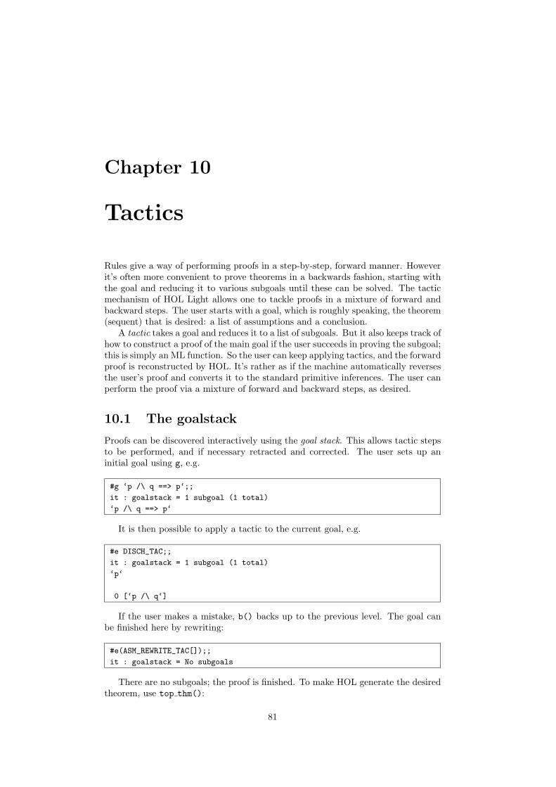
Chapter 10
Tactics
Rules give a way of performing proofs in a step-by-step, forward manner. Howeverit’s often more convenient to prove theorems in a backwards fashion, starting withthe goal and reducing it to various subgoals until these can be solved. The tacticmechanism of HOL Light allows one to tackle proofs in a mixture of forward andbackward steps. The user starts with a goal, which is roughly speaking, the theorem(sequent) that is desired: a list of assumptions and a conclusion.
A tactic takes a goal and reduces it to a list of subgoals. But it also keeps track ofhow to construct a proof of the main goal if the user succeeds in proving the subgoal;this is simply an ML function. So the user can keep applying tactics, and the forwardproof is reconstructed by HOL. It’s rather as if the machine automatically reversesthe user’s proof and converts it to the standard primitive inferences. The user canperform the proof via a mixture of forward and backward steps, as desired.
10.1 The goalstack
Proofs can be discovered interactively using the goal stack. This allows tactic stepsto be performed, and if necessary retracted and corrected. The user sets up aninitial goal using g, e.g.
#g ‘p /\ q ==> p‘;;
it : goalstack = 1 subgoal (1 total)
‘p /\ q ==> p‘
It is then possible to apply a tactic to the current goal, e.g.
#e DISCH_TAC;;
it : goalstack = 1 subgoal (1 total)
‘p‘
0 [‘p /\ q‘]
If the user makes a mistake, b() backs up to the previous level. The goal canbe finished here by rewriting:
#e(ASM_REWRITE_TAC[]);;
it : goalstack = No subgoals
There are no subgoals; the proof is finished. To make HOL generate the desiredtheorem, use top thm():
81

82 CHAPTER 10. TACTICS
#top_thm();;
it : thm = |- p /\ q ==> p
If a tactic splits a goal into more than one subgoal, they are presented one at atime. When one subgoal is solved the next unsolved one is presented. For example:
#g ‘p /\ q /\ r ==> q /\ p /\ r‘;;
it : goalstack = 1 subgoal (1 total)
‘p /\ q /\ r ==> q /\ p /\ r‘
#e DISCH_TAC;;
it : goalstack = 1 subgoal (1 total)
‘q /\ p /\ r‘
0 [‘p /\ q /\ r‘]
#e CONJ_TAC;;
it : goalstack = 2 subgoals (2 total)
‘p /\ r‘
0 [‘p /\ q /\ r‘]
‘q‘
0 [‘p /\ q /\ r‘]
#e(ASM_REWRITE_TAC[]);;
it : goalstack = 1 subgoal (1 total)
‘p /\ r‘
0 [‘p /\ q /\ r‘]
#e CONJ_TAC;;
it : goalstack = 2 subgoals (2 total)
‘r‘
0 [‘p /\ q /\ r‘]
‘p‘
0 [‘p /\ q /\ r‘]
#e(ASM_REWRITE_TAC[]);;
it : goalstack = 1 subgoal (1 total)
‘r‘
0 [‘p /\ q /\ r‘]
#e(ASM_REWRITE_TAC[]);;
it : goalstack = No subgoals
Effectively, the user is always at a point in the fringe of the partial proof tree.The position can be rotated by n goals by doing r n.

10.2. BASIC TACTICS 83
10.2 Basic tactics
The most basic tactics correspond to the basic logical derived rules, but workingthe other way round. We have seen some of them above. For example, where CONJtakes two theorems and gives their conjunction, the tactic CONJ TAC breaks down aconjunctive goal and returns the two subgoals. Similarly DISJ1 TAC reduces a goalwith conclusion p ∨ q to one with conclusion p, i.e. allows the user to decide toprove the first disjunct. Again, DISCH TAC reverses the effect of the rule DISCH, i.e.it reduces a goal Γ `? p⇒ q to Γ ∪ {p} `? q.
Tactics are especially useful for using rules like CHOOSE. If one has a theorem` ∃x. p, then one can just put p into the assumptions of the goal using CHOOSE TAC.Thereafter, it is as if one had picked some x such that p holds and can use it tosolve the goal; HOL handles the appropriate application of CHOOSE.
The tactics MP TAC and MATCH MP are a bit tricker to understand, in that it’snot quite so clear how they amount to reversals of MP and MATCH MP. In fact theirbehaviour is quite different, going well beyond one performing matching and onenot. Given a goal with conclusion q and a theorem that after matching is of theform p⇒ q, then MATCH MP TAC reduces the goal to p. For example:
#g ‘0 <= SUC n‘;;
it : goalstack = 1 subgoal (1 total)
‘0 <= SUC n‘
#e(MATCH_MP_TAC LT_IMP_LE);;
it : goalstack = 1 subgoal (1 total)
‘0 < SUC n‘
MP TAC, on the other hand, simply places the theorem as an antecedent of thegoal:
#g ‘0 <= SUC n‘;;
it : goalstack = 1 subgoal (1 total)
‘0 <= SUC n‘
#e(MP_TAC LT_IMP_LE);;
it : goalstack = 1 subgoal (1 total)
‘(!m n. m < n ==> m <= n) ==> 0 <= SUC n‘
However this effect can be quite useful, since it’s often more convenient to dothings like rewrite on the conclusion of a goal, rather than the assumptions.
None of the tactics we have considered so far solves goals completely. The mostprimitive tactic that does is ACCEPT TAC, which is used with a theorem with thesame conclusion as the goal. A slightly more general version, MATCH ACCEPT TAC,will do some matching, e.g.
#g ‘x + 1 = 1 + x‘;;
it : goalstack = 1 subgoal (1 total)
‘x + 1 = 1 + x‘
#e(MATCH_ACCEPT_TAC ADD_SYM);;
it : goalstack = No subgoals
Another group of tactics can be created from conversions, using CONV TAC. Thiscreates a tactic that applies the given conversion to the goal, e.g.

84 CHAPTER 10. TACTICS
#g ‘(\x. x + 1) 2 = 3‘;;
it : goalstack = 1 subgoal (1 total)
‘(\x. x + 1) 2 = 3‘
#e(CONV_TAC(ONCE_DEPTH_CONV BETA_CONV));;
it : goalstack = 1 subgoal (1 total)
‘2 + 1 = 3‘
If the conversion transforms the goal to T, the tactic mechanism accepts that assolving the goal, rather than presenting T as the subgoal, e.g.
#g ‘2 + 1 = 3‘;;
it : goalstack = 1 subgoal (1 total)
‘2 + 1 = 3‘
#e(CONV_TAC NUM_REDUCE_CONV);;
it : goalstack = No subgoals
The rewriting conversions are also all used as tactics, e.g. REWRITE TAC. Thesame names prefixed with ASM also use the assumptions of the current goal asrewrites.
10.3 Tacticals
Just as basic conversions are built up into composite ones by conversionals, sotactics are built up via tacticals. For example the infix THEN executes two tactics insequence. Once a proof has been found using the subgoal mechanism, it’s commonto plug all the steps into one tactic using THEN, e.g.
#g ‘!m n p. m * (n + p) = (m * n) + (m * p)‘;;
it : goalstack = 1 subgoal (1 total)
‘!m n p. m * (n + p) = m * n + m * p‘
#e(GEN_TAC THEN
INDUCT_TAC THEN
ASM_REWRITE_TAC[ADD; MULT_CLAUSES; ADD_ASSOC]);;
it : goalstack = No subgoals
If the first tactic sequenced by THEN generates more than one subgoal, then thesecond tactic is applied to all of them. If different tactics are used for each subgoal,they can be put into a list and sequenced using THENL, e.g.
#g ‘p ==> p /\ (1 = 1)‘;;
it : goalstack = 1 subgoal (1 total)
‘p ==> p /\ (1 = 1)‘
#e(DISCH_TAC THEN
CONJ_TAC THENL
[ASM_REWRITE_TAC[];
ACCEPT_TAC (REFL ‘1‘)]);;
it : goalstack = No subgoals
Tactics can be executed repeatedly by REPEAT, and there are various other usefultacticals.
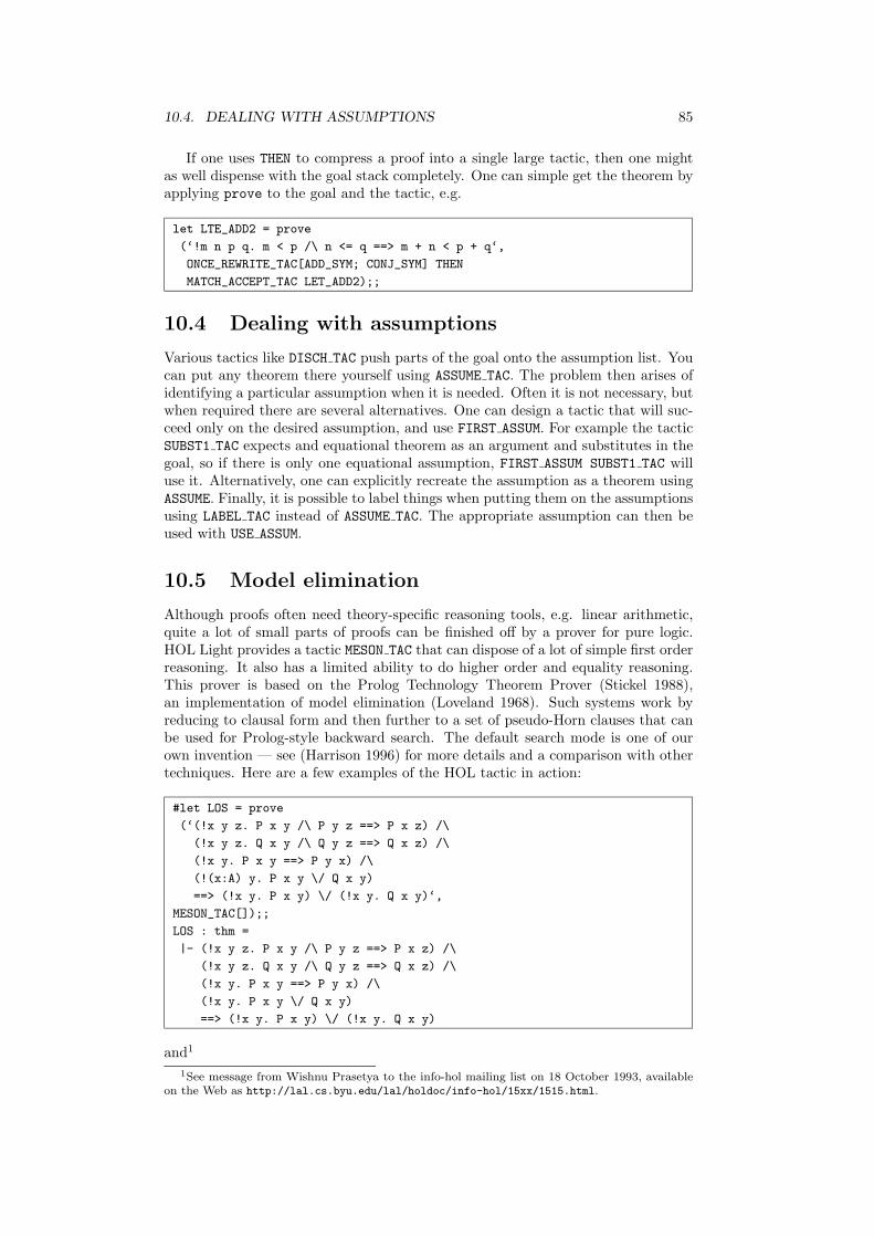
10.4. DEALING WITH ASSUMPTIONS 85
If one uses THEN to compress a proof into a single large tactic, then one mightas well dispense with the goal stack completely. One can simple get the theorem byapplying prove to the goal and the tactic, e.g.
let LTE_ADD2 = prove
(‘!m n p q. m < p /\ n <= q ==> m + n < p + q‘,
ONCE_REWRITE_TAC[ADD_SYM; CONJ_SYM] THEN
MATCH_ACCEPT_TAC LET_ADD2);;
10.4 Dealing with assumptions
Various tactics like DISCH TAC push parts of the goal onto the assumption list. Youcan put any theorem there yourself using ASSUME TAC. The problem then arises ofidentifying a particular assumption when it is needed. Often it is not necessary, butwhen required there are several alternatives. One can design a tactic that will suc-ceed only on the desired assumption, and use FIRST ASSUM. For example the tacticSUBST1 TAC expects and equational theorem as an argument and substitutes in thegoal, so if there is only one equational assumption, FIRST ASSUM SUBST1 TAC willuse it. Alternatively, one can explicitly recreate the assumption as a theorem usingASSUME. Finally, it is possible to label things when putting them on the assumptionsusing LABEL TAC instead of ASSUME TAC. The appropriate assumption can then beused with USE ASSUM.
10.5 Model elimination
Although proofs often need theory-specific reasoning tools, e.g. linear arithmetic,quite a lot of small parts of proofs can be finished off by a prover for pure logic.HOL Light provides a tactic MESON TAC that can dispose of a lot of simple first orderreasoning. It also has a limited ability to do higher order and equality reasoning.This prover is based on the Prolog Technology Theorem Prover (Stickel 1988),an implementation of model elimination (Loveland 1968). Such systems work byreducing to clausal form and then further to a set of pseudo-Horn clauses that canbe used for Prolog-style backward search. The default search mode is one of ourown invention — see (Harrison 1996) for more details and a comparison with othertechniques. Here are a few examples of the HOL tactic in action:
#let LOS = prove
(‘(!x y z. P x y /\ P y z ==> P x z) /\
(!x y z. Q x y /\ Q y z ==> Q x z) /\
(!x y. P x y ==> P y x) /\
(!(x:A) y. P x y \/ Q x y)
==> (!x y. P x y) \/ (!x y. Q x y)‘,
MESON_TAC[]);;
LOS : thm =
|- (!x y z. P x y /\ P y z ==> P x z) /\
(!x y z. Q x y /\ Q y z ==> Q x z) /\
(!x y. P x y ==> P y x) /\
(!x y. P x y \/ Q x y)
==> (!x y. P x y) \/ (!x y. Q x y)
and1
1See message from Wishnu Prasetya to the info-hol mailing list on 18 October 1993, availableon the Web as http://lal.cs.byu.edu/lal/holdoc/info-hol/15xx/1515.html.
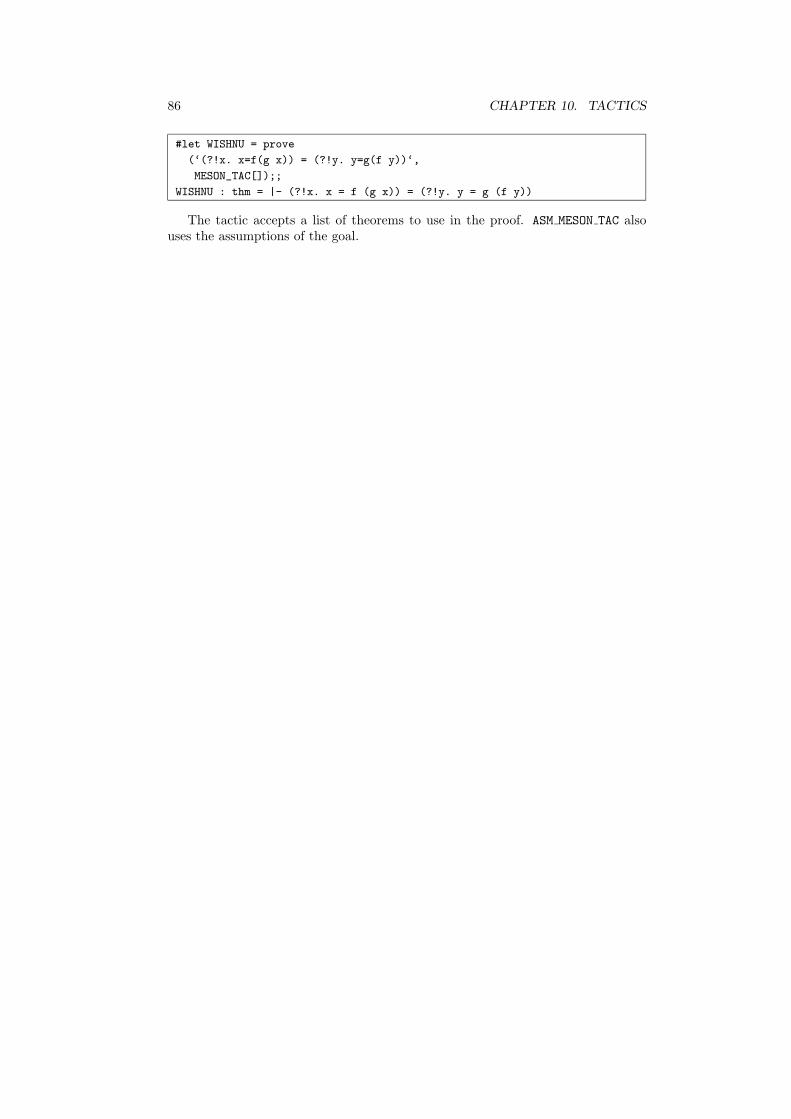
86 CHAPTER 10. TACTICS
#let WISHNU = prove
(‘(?!x. x=f(g x)) = (?!y. y=g(f y))‘,
MESON_TAC[]);;
WISHNU : thm = |- (?!x. x = f (g x)) = (?!y. y = g (f y))
The tactic accepts a list of theorems to use in the proof. ASM MESON TAC alsouses the assumptions of the goal.
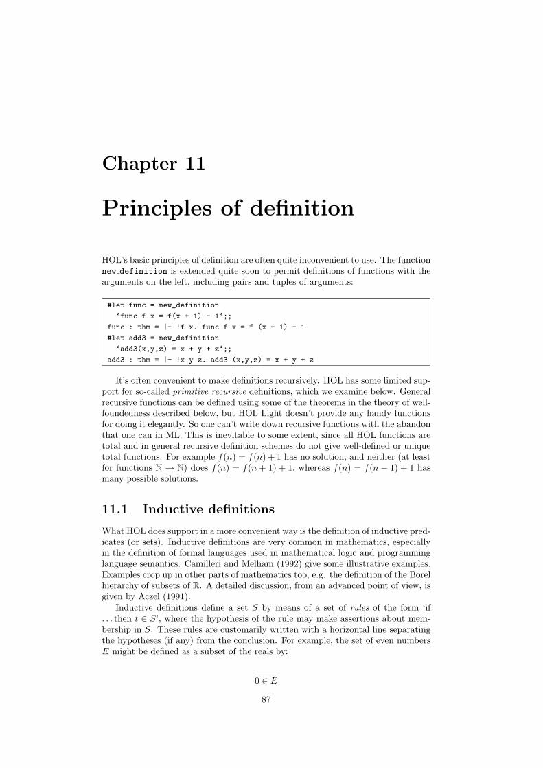
Chapter 11
Principles of definition
HOL’s basic principles of definition are often quite inconvenient to use. The functionnew definition is extended quite soon to permit definitions of functions with thearguments on the left, including pairs and tuples of arguments:
#let func = new_definition
‘func f x = f(x + 1) - 1‘;;
func : thm = |- !f x. func f x = f (x + 1) - 1
#let add3 = new_definition
‘add3(x,y,z) = x + y + z‘;;
add3 : thm = |- !x y z. add3 (x,y,z) = x + y + z
It’s often convenient to make definitions recursively. HOL has some limited sup-port for so-called primitive recursive definitions, which we examine below. Generalrecursive functions can be defined using some of the theorems in the theory of well-foundedness described below, but HOL Light doesn’t provide any handy functionsfor doing it elegantly. So one can’t write down recursive functions with the abandonthat one can in ML. This is inevitable to some extent, since all HOL functions aretotal and in general recursive definition schemes do not give well-defined or uniquetotal functions. For example f(n) = f(n) + 1 has no solution, and neither (at leastfor functions N → N) does f(n) = f(n + 1) + 1, whereas f(n) = f(n − 1) + 1 hasmany possible solutions.
11.1 Inductive definitions
What HOL does support in a more convenient way is the definition of inductive pred-icates (or sets). Inductive definitions are very common in mathematics, especiallyin the definition of formal languages used in mathematical logic and programminglanguage semantics. Camilleri and Melham (1992) give some illustrative examples.Examples crop up in other parts of mathematics too, e.g. the definition of the Borelhierarchy of subsets of R. A detailed discussion, from an advanced point of view, isgiven by Aczel (1991).
Inductive definitions define a set S by means of a set of rules of the form ‘if. . . then t ∈ S’, where the hypothesis of the rule may make assertions about mem-bership in S. These rules are customarily written with a horizontal line separatingthe hypotheses (if any) from the conclusion. For example, the set of even numbersE might be defined as a subset of the reals by:
0 ∈ E
87

88 CHAPTER 11. PRINCIPLES OF DEFINITION
n ∈ E(n+ 2) ∈ E
Read literally, such a definition merely places some constraints on the set E,asserting its ‘closure’ under the rules, and does not, in general, determine it uniquely.For example, the set of even numbers satisfies the above, but so does the set ofnatural numbers, the set of integers, the set of rational numbers and even the thewhole set of real numbers! But implicit in writing a definition like this is that Eis the least set which is closed under the rules. It is when understood in this sensethat the above defines the even numbers.
This convention, however, needs to be justified by showing that there is a leastset closed under the rules. A good try is to consider the set of all sets whichare closed under the rules, and take their intersection. If only we knew that thisintersection was closed under the rules, then it would certainly be the least suchset. But in general we don’t know that, as the following example illustrates:
n 6∈ En ∈ E
There are no sets at all closed under this rule! However it turns out that a simplesyntactic restriction on the rules is enough to guarantee that the intersection isclosed under the rules. Crudely speaking, the hypotheses must make only ‘positive’assertions about membership in S. To state this precisely, observe that we cancollect together all the rules in a single assertion of the form:
∀x. P [S, x]⇒ x ∈ S
The following example for the even numbers should be a suitable paradigm toindicate how:
∀n. (n = 0 ∨ ∃m. n = m+ 2 ∧m ∈ E)⇒ n ∈ E
If we make the abbreviation f(S) = {x | P [S, x]} the assertion can be writtenf(S) ⊆ S. Our earlier plan was to take the intersection of all subsets S whichhave this property, and hope that the intersection too is closed under the rules.A sufficient condition for this is given in the following fixpoint theorem due toKnaster (1927) and Tarski (1955) (which holds for an arbitrary complete lattice):if f : ℘(X)→ ℘(X) is monotone, i.e. for any S ⊆ X and T ⊆ X
S ⊆ T ⇒ f(S) ⊆ f(T )
then if we define
F =⋂{S ⊆ X | f(S) ⊆ S}
not only is f(F ) ⊆ F but F is actually a fixpoint of f , i.e. f(F ) = F . HOL Lightcan take an inductive definition and generally manage to prove monotonicity foritself, providing the user with three useful theorems. The first says that the definedset is closed under the rules, the second that it is the least set closed under therules, and the third gives a case analysis theorem saying that everything in the setis generated by applying the rules to something else in the set. For example, wecan define finiteness of sets (or, viewed as a set, the set of all finite sets) as follows:

11.2. FREE RECURSIVE TYPES 89
#let finite_RULES,finite_INDUCT,finite_CASES =
new_inductive_definition
‘finite {} /\
!x s. finite s ==> finite (x INSERT s)‘;;
Warning: inventing type variables
finite_RULES : thm =
|- finite EMPTY /\ (!x s. finite s ==> finite (x INSERT s))
finite_INDUCT : thm =
|- !finite’. finite’ EMPTY /\ (!x s. finite’ s ==> finite’ (x INSERT s))
==> (!a. finite a ==> finite’ a)
finite_CASES : thm =
|- !a. finite a = (a = EMPTY) \/ (?x s. (a = x INSERT s) /\ finite s)
HOL Light allows the user to define mutually inductive relations. For examplehere are predicates for evenness and oddity:
#let even_odd_RULES,even_odd_INDUCT,even_odd_CASES =
new_inductive_definition
‘even 0 /\
(!n. even(n) ==> odd(n + 1)) /\
(!n. odd(n) ==> even(n + 1))‘;;
even_odd_RULES : thm =
|- even 0 /\ (!n. even n ==> odd (n + 1)) /\ (!n. odd n ==> even (n + 1))
even_odd_INDUCT : thm =
|- !odd’ even’.
even’ 0 /\
(!n. even’ n ==> odd’ (n + 1)) /\
(!n. odd’ n ==> even’ (n + 1))
==> (!a0. odd a0 ==> odd’ a0) /\ (!a1. even a1 ==> even’ a1)
even_odd_CASES : thm =
|- (!a0. odd a0 = (?n. (a0 = n + 1) /\ even n)) /\
(!a1. even a1 = (a1 = 0) \/ (?n. (a1 = n + 1) /\ odd n))
The induction theorem can be applied conveniently during backward proof usingthe tactical RULE INDUCT THEN, or in simple cases just with MATCH MP TAC.
11.2 Free recursive types
HOL Light’s primitive type definition facility is rather awkward to work with. Oneof the most useful, and complicated, derived rules in HOL Light allows one to definerecursive types much as in CAML, even using a similar syntax. There are somerestrictions; for example a function space involving the type being defined cannot beused. However types can be defined mutually recursively and can involve instancesof previously defined type constructors. The primitive function is define type, andit always returns two theorems, the first a kind of induction theorem for the newtype, the second a justification of definition by primitive recursion. For example wecan define binary trees:
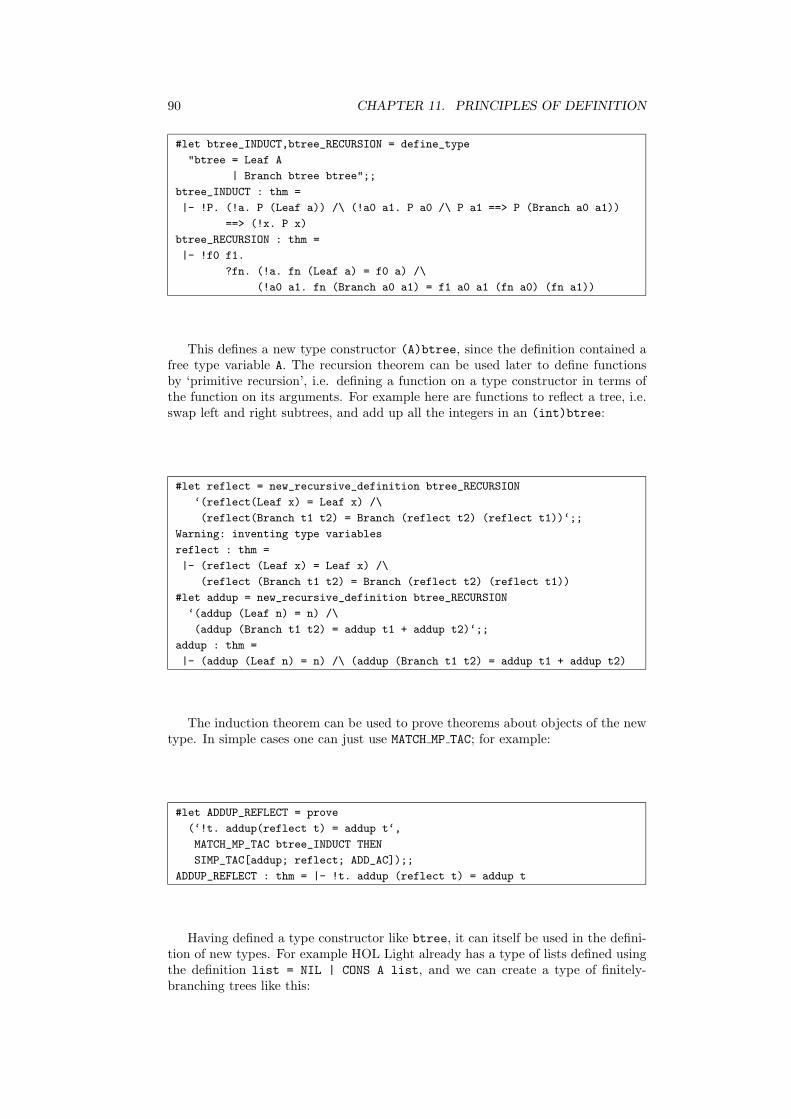
90 CHAPTER 11. PRINCIPLES OF DEFINITION
#let btree_INDUCT,btree_RECURSION = define_type
"btree = Leaf A
| Branch btree btree";;
btree_INDUCT : thm =
|- !P. (!a. P (Leaf a)) /\ (!a0 a1. P a0 /\ P a1 ==> P (Branch a0 a1))
==> (!x. P x)
btree_RECURSION : thm =
|- !f0 f1.
?fn. (!a. fn (Leaf a) = f0 a) /\
(!a0 a1. fn (Branch a0 a1) = f1 a0 a1 (fn a0) (fn a1))
This defines a new type constructor (A)btree, since the definition contained afree type variable A. The recursion theorem can be used later to define functionsby ‘primitive recursion’, i.e. defining a function on a type constructor in terms ofthe function on its arguments. For example here are functions to reflect a tree, i.e.swap left and right subtrees, and add up all the integers in an (int)btree:
#let reflect = new_recursive_definition btree_RECURSION
‘(reflect(Leaf x) = Leaf x) /\
(reflect(Branch t1 t2) = Branch (reflect t2) (reflect t1))‘;;
Warning: inventing type variables
reflect : thm =
|- (reflect (Leaf x) = Leaf x) /\
(reflect (Branch t1 t2) = Branch (reflect t2) (reflect t1))
#let addup = new_recursive_definition btree_RECURSION
‘(addup (Leaf n) = n) /\
(addup (Branch t1 t2) = addup t1 + addup t2)‘;;
addup : thm =
|- (addup (Leaf n) = n) /\ (addup (Branch t1 t2) = addup t1 + addup t2)
The induction theorem can be used to prove theorems about objects of the newtype. In simple cases one can just use MATCH MP TAC; for example:
#let ADDUP_REFLECT = prove
(‘!t. addup(reflect t) = addup t‘,
MATCH_MP_TAC btree_INDUCT THEN
SIMP_TAC[addup; reflect; ADD_AC]);;
ADDUP_REFLECT : thm = |- !t. addup (reflect t) = addup t
Having defined a type constructor like btree, it can itself be used in the defini-tion of new types. For example HOL Light already has a type of lists defined usingthe definition list = NIL | CONS A list, and we can create a type of finitely-branching trees like this:

11.2. FREE RECURSIVE TYPES 91
#let xtree_INDUCTION,xtree_RECURSION = define_type
"xtree = Lf A
| Br (xtree list)";;
xtree_INDUCTION : thm =
|- !P0 P1.
(!a. P0 (Lf a)) /\
(!a. P1 a ==> P0 (Br a)) /\
P1 [] /\
(!a0 a1. P0 a0 /\ P1 a1 ==> P1 (CONS a0 a1))
==> (!x0. P0 x0) /\ (!x1. P1 x1)
xtree_RECURSION : thm =
|- !f0 f1 f2 f3.
?fn0 fn1.
(!a. fn1 (Lf a) = f0 a) /\
(!a. fn1 (Br a) = f1 a (fn0 a)) /\
(fn0 [] = f2) /\
(!a0 a1. fn0 (CONS a0 a1) = f3 a0 a1 (fn1 a0) (fn0 a1))
The induction and recursion theorems are as if the list constructor had beendefined mutually recursively, but it uses the standard type of lists.

92 CHAPTER 11. PRINCIPLES OF DEFINITION

Chapter 12
Mathematical theories
To prove theorems in HOL Light, one needs a reasonable grasp of the theoremproving infrastructure. But equally important is knowing what has already beenproved, and what the theorem one is after has been called. The following is not anexhaustive list, but gives some of the main theorems, grouped according to subjectarea. The following gives only a general overview; the reader should browse thesource files to become more familiar with what is available.
12.1 Pairs
There is a type constructor prod that constructs Cartesian product types. In theconcrete syntax of the type parser it is written as #. For example num # num isthe type of pairs of natural numbers. Larger tuples can be built by iterating thepairing operation; the type constructor and the term function that constructs pairs(the infix comma) are both right associative. Destructors FST and SND are defined.Some of the main theorems about pairs are:
PAIR_EQ = |- !x y a b. (x,y = a,b) = (x = a) /\ (y = b)
PAIR_SURJECTIVE = |- !p. ?x y. p = x,y
FST = |- !x y. FST (x,y) = x
SND = |- !x y. SND (x,y) = y
PAIR = |- !x. FST x,SND x = x
pair_INDUCT = |- (!x y. P (x,y)) ==> (!p. P p)
pair_RECURSION = |- !PAIR’. ?fn. !a0 a1. fn (a0,a1) = PAIR’ a0 a1
The last two are chosen as if pairs had been defined as a recursive type, thoughin fact they logically precede other recursive types.
12.2 Natural numbers
The type of natural numbers is carved out, using an inductive definition, from theinfinite type ind. The Peano axioms are derived from the definition and the axiomsof infinity. As with pairs, two theorems mimic those resulting from recursive typedefinitions, allowing proofs by induction and definitions by primitive recursion:
93

94 CHAPTER 12. MATHEMATICAL THEORIES
num_INDUCTION = |- !P. P 0 /\ (!n. P n ==> P (SUC n)) ==> (!n. P n)
num_RECURSION = |- !e f. ?fn. (fn 0 = e) /\ (!n. fn (SUC n) = f (fn n) n)
The latter is used to define most of the arithmetic operations, including thecomparisons:
ADD = |- (!n. 0 + n = n) /\ (!m n. SUC m + n = SUC (m + n))
MULT = |- (!n. 0 * n = 0) /\ (!m n. SUC m * n = m * n + n)
EXP = |- (!m. m EXP 0 = 1) /\ (!m n. m EXP SUC n = m * m EXP n)
LE = |- (!m. m <= 0 = m = 0) /\(!m n. m <= SUC n = (m = SUC n) \/ m <= n)
LT = |- (!m. m < 0 = F) /\ (!m n. m < SUC n = (m = n) \/ m < n)
EVEN = |- (EVEN 0 = T) /\ (!n. EVEN (SUC n) = ~EVEN n)
ODD = |- (ODD 0 = F) /\ (!n. ODD (SUC n) = ~ODD n)
Numerals are prettyprinted forms of an internal binary representation using twoconstants:
BIT0 = |- BIT0 n = n + n
BIT1 = |- BIT1 n = SUC(n + n)
The rather artificial definition of the second is because multiplication (whichuses numeral 1 in its definition) has not yet been defined. Now these constants aresufficient to express any number in binary. For example, we implement 37 as:
NUMERAL (BIT1 (BIT0 (BIT1 (BIT0 (BIT0 (BIT1 _0))))))
The reader may wonder why we use the constant NUMERAL at all, instead of justusing BIT0, BIT1 and 0. The reason is that in that case one number becomes asubterm of another (e.g. 1 is a subterm of 2), which can lead to some surprising acci-dental rewrites. Besides, the NUMERAL constant is a useful tag for the prettyprinter.
The parser and printer transformations established, the theory of natural num-bers can now be developed as usual. Most of the arithmetic operations are definedby primitive recursion, indicating a simple evaluation strategy for unary notation.For example one can evaluate 3 + 5 as follows:
3 + 5SUC 2 + 5SUC (2 + 5)SUC (SUC 1 + 5)SUC (SUC (1 + 5))SUC (SUC (SUC 0 + 5)))SUC (SUC (SUC (0 + 5)))SUC (SUC (SUC 5))SUC (SUC 6)SUC 78

12.3. LISTS 95
But many of them have an almost equally direct strategy in terms of our binarynotation.1 For example the following theorems, easily proved, can be used directlyas rewrite rules to perform arithmetic evaluation.
|- (!n. SUC (NUMERAL n) = NUMERAL (SUC n)) /\(SUC _0 = BIT1 _0) /\(!n. SUC (BIT0 n) = BIT1 n) /\(!n. SUC (BIT1 n) = BIT0 (SUC n))
or
|- (!m n. (NUMERAL m = NUMERAL n) = (m = n)) /\((_0 = _0) = T) /\(!n. (BIT0 n = _0) = (n = _0)) /\(!n. (BIT1 n = _0) = F) /\(!n. (_0 = BIT0 n) = (_0 = n)) /\(!n. (_0 = BIT1 n) = F) /\(!m n. (BIT0 m = BIT0 n) = (m = n)) /\(!m n. (BIT0 m = BIT1 n) = F) /\(!m n. (BIT1 m = BIT0 n) = F) /\(!m n. (BIT1 m = BIT1 n) = (m = n))
Most arithmetic operations can be implemented as a set of rewrite rules likethe above, and applied using the standard rewriting mechanism. A suite of suchrewrites is collected together into a single rewrite rule ARITH that will evaluate mostground expressions using just the standard rewriting mechanism. For example:
#let conv = PURE_REWRITE_CONV[ARITH];;conv : conv = <fun>#conv ‘12345 * 12345‘;;it : thm = |- 12345 * 12345 = 152399025
However, a few operations are hard to evaluate efficiently with the standardrewriting mechanism; even ARITH_SUB is a bit inefficient, since the same conditionis tested repeatedly. Therefore we also provide a full suite of conversions, and collectthem together as NUM RED CONV and NUM REDUCE CONV.
12.3 Lists
A HOL recursive type of lists is defined, and various standard list combinatorsdefined by recursion. These often have the same names as their CAML counterparts,but in upper case.
HD = |- HD (CONS h t) = h
TL = |- TL (CONS h t) = t
APPEND =|- (!l. APPEND [] l = l) /\
(!h t l. APPEND (CONS h t) l = CONS h (APPEND t l))
1Another nice example, though we don’t actually implement it, is the GCD function. Knuth(1969) gives a simple algorithm based on gcd(2m, 2n) = 2gcd(m,n), gcd(2m+ 1, 2n) = gcd(2m+1, n) and gcd(2m+1, 2n+1) = gcd(m−n, 2n+1). This outperforms Euclid’s method on machineswhere bitwise operations are relatively efficient; our in-logic implementation would surely exhibitthe same characteristics even if our ‘bits’ are rather large!

96 CHAPTER 12. MATHEMATICAL THEORIES
REVERSE =|- (REVERSE [] = []) /\ (REVERSE (CONS x l) = APPEND (REVERSE l) [x])
LENGTH =|- (LENGTH [] = 0) /\ (!h t. LENGTH (CONS h t) = SUC (LENGTH t))
MAP = |- (!f. MAP f [] = []) /\(!f h t. MAP f (CONS h t) = CONS (f h) (MAP f t))
LAST = |- LAST (CONS h t) = (if t = [] then h else LAST t)
REPLICATE = |- (REPLICATE 0 x = []) /\(REPLICATE (SUC n) x = CONS x (REPLICATE n x))
NULL = |- (NULL [] = T) /\ (NULL (CONS h t) = F)
FORALL = |- (FORALL P [] = T) /\(FORALL P (CONS h t) = P h /\ FORALL P t)
EX = |- (EX P [] = F) /\ (EX P (CONS h t) = P h \/ EX P t)
ITLIST =|- (ITLIST f [] b = b) /\ (ITLIST f (CONS h t) b = f h (ITLIST f t b))
MEM = |- (MEM x [] = F) /\ (MEM x (CONS h t) = (x = h) \/ MEM x t)
A somewhat ad hoc collection of facts about these functions is collected, forexample:
APPEND_ASSOC = |- !l m n. APPEND l (APPEND m n) = APPEND (APPEND l m) n
LENGTH_APPEND = |- !l m. LENGTH (APPEND l m) = LENGTH l + LENGTH m
LENGTH_MAP = |- !l f. LENGTH (MAP f l) = LENGTH l
REVERSE_REVERSE = |- !l. REVERSE (REVERSE l) = l
MAP_o = |- !f g l. MAP (g o f) l = MAP g (MAP f l)
NOT_EX = |- !P l. ~EX P l = FORALL (\x. ~P x) l
12.4 Well-founded relations
Wellfoundedness of a binary relation can be expressed in many equivalent ways.HOL Light includes a definition of wellfoundedness and a proof that it equivalentto several other important properties, like the admissibility of complete inductionand wellfounded recursion. For example, the last theorem below, which also has aconverse, says that one can define recursive functions provided the value of f(x) isdefined in terms of f(y) for y below x in the wellfounded ordering.
WF =|- WF (<<) = (!P. (?x. P x) ==> (?x. P x /\ (!y. y << x ==> ~P y)))

12.5. REAL NUMBERS 97
WF_IND =|- WF (<<) = (!P. (!x. (!y. y << x ==> P y) ==> P x) ==> (!x. P x))
WF_DCHAIN = |- WF (<<) = ~(?s. !n. s (SUC n) << s n)
WF_REC =|- WF (<<)
==> (!H. (!f g x. (!z. z << x ==> (f z = g z)) ==> (H f x = H g x))==> (?f. !x. f x = H f x))
12.5 Real numbers
HOL Light constructs the real numbers and then proves various properties of them.Algebraic trivialities include:
REAL_OF_NUM_SUB : thm = |- !m n. m <= n ==> (&n - &m = &(n - m))
REAL_ADD_RID : thm = |- !x. x + &0 = x
REAL_LT_IMP_LE : thm = |- !x y. x < y ==> x <= y
REAL_LT_LADD_IMP : thm = |- !x y z. y < z ==> x + y < x + z
REAL_LT_LNEG : thm = |- !x y. -- x < y = &0 < x + y
REAL_ABS_TRIANGLE : thm = |- !x y. abs (x + y) <= abs x + abs y
REAL_ABS_MUL : thm = |- !x y. abs (x * y) = abs x * abs y
REAL_INV_MUL : thm = |- !x y. inv (x * y) = inv x * inv y
Note that the inverse is defined with 0−1 = 0. Most theorems not involvingmultiplication can be proved automatically using REAL ARITH or the tactic formREAL ARITH TAC:
#REAL_ARITH ‘abs(x) < y ==> x < y‘;;
it : thm = |- abs x < y ==> x < y
The key higher-order property of the reals asserts that any nonempty boundedset of reals has a least upper bound:
#REAL_COMPLETE;;
it : thm =
|- !P. (?x. P x) /\ (?M. !x. P x ==> x <= M)
==> (?M. (!x. P x ==> x <= M) /\
(!M’. (!x. P x ==> x <= M’) ==> M <= M’))
There is not much real analysis in the basic system, but there is a reasonabledevelopment included with the examples.
12.6 Integers
A theory of integers is also available, with theorems named by analogy with thereals, e.g. INT LT IMP LE rather than REAL LT IMP LE. Similarly, there is a decisionprocedure for linear integer arithmetic called INT ARITH.
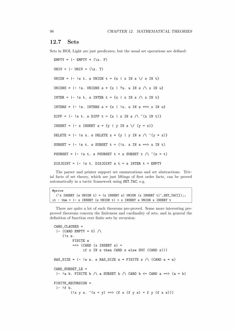
98 CHAPTER 12. MATHEMATICAL THEORIES
12.7 Sets
Sets in HOL Light are just predicates, but the usual set operations are defined:
EMPTY = |- EMPTY = (\x. F)
UNIV = |- UNIV = (\x. T)
UNION = |- !s t. s UNION t = {x | x IN s \/ x IN t}
UNIONS = |- !s. UNIONS s = {x | ?u. u IN s /\ x IN u}
INTER = |- !s t. s INTER t = {x | x IN s /\ x IN t}
INTERS = |- !s. INTERS s = {x | !u. u IN s ==> x IN u}
DIFF = |- !s t. s DIFF t = {x | x IN s /\ ~(x IN t)}
INSERT = |- x INSERT s = {y | y IN s \/ (y = x)}
DELETE = |- !s x. s DELETE x = {y | y IN s /\ ~(y = x)}
SUBSET = |- !s t. s SUBSET t = (!x. x IN s ==> x IN t)
PSUBSET = |- !s t. s PSUBSET t = s SUBSET t /\ ~(s = t)
DISJOINT = |- !s t. DISJOINT s t = s INTER t = EMPTY
The parser and printer support set enumerations and set abstractions. Triv-ial facts of set theory, which are just liftings of first order facts, can be provedautomatically in a tactic framework using SET TAC, e.g.
#prove
(‘x INSERT (s UNION t) = (x INSERT s) UNION (x INSERT t)‘,SET_TAC[]);;
it : thm = |- x INSERT (s UNION t) = x INSERT s UNION x INSERT t
There are quite a lot of such theorems pre-proved. Some more interesting pre-proved theorems concern the finiteness and cardinality of sets, and in general thedefinition of function over finite sets by recursion:
CARD_CLAUSES =|- (CARD EMPTY = 0) /\
(!x s.FINITE s==> (CARD (x INSERT s) =
if x IN s then CARD s else SUC (CARD s)))
HAS_SIZE = |- !s n. s HAS_SIZE n = FINITE s /\ (CARD s = n)
CARD_SUBSET_LE =|- !a b. FINITE b /\ a SUBSET b /\ CARD b <= CARD a ==> (a = b)
FINITE_RECURSION =|- !f b.
(!x y s. ~(x = y) ==> (f x (f y s) = f y (f x s)))

12.7. SETS 99
==> (ITSET f EMPTY b = b) /\(!x s.
FINITE s==> (ITSET f (x INSERT s) b =
if x IN s then ITSET f s b else f x (ITSET f s b)))

100 CHAPTER 12. MATHEMATICAL THEORIES

Chapter 13
Examples
A few examples are included in Examples directory. These just give some indicationof how the system can be used. They aren’t held up as particularly good examplesexploiting HOL Light’s facilities; indeed many of them are crudely ported fromolder versions of HOL. A few of them might be useful to some readers, but they aregenerally not polished or documented.
• analysis.ml is a development of elementary real analysis, e.g. sequences,series, limits, continuity, differentiation and integration.
• lagrange.ml shows how to prove some numerical identities using orderedrewriting and/or decision procedures.
• mizar.ml is a system for writing HOL proofs in a more readable declarativestyle based on Trybulec’s Mizar system (Rudnicki 1992).
• prog.ml is a simple embedding of the semantics of a toy imperative program-ming language, derivation of weakest preconditions and Floyd-Hoare rules,and a tactic that performs verification condition generation on an annotatedprogram.
• rectypes.ml defines a wide variety of (mutual, nested) recursive types.
• reduct.ml defines some basic notions for reductions, e.g. confluence, nor-malization, and proves a few theorems like Newman’s Lemma. It requiresrstc.ml to have been loaded first.
• rstc.ml defines various combinations of reflexive, symmetric and transitiveclosures of binary relations, and proves a comprehensive set of theorems aboutthem.
• transc.ml defines and proves properties of the elementary transcendentalfunctions like exp, sin and ln. It requires analysis.ml to have been loadedfirst.
• wo.ml proves some important version of the Axiom of Choice, e.g. the wellorder-ing principle and Zorn’s Lemma.
101

102 CHAPTER 13. EXAMPLES

Appendix A
Compatibility with otherHOLs
Here is a brief list of some of the major incompatibilities with other versions ofHOL:
• CAML, the underlying ML is different from previous HOL versions, some-where between ‘Classic ML’ and Standard ML.
• There is no theory mechanism; every theorem is just bound to an ML name.It is possible to save and load theorems via CAML primitives, but this isnot recommended since it subverts the usual mechanisms for constructingelements of the thm type.
• Parsing status is orthogonal to whether an identifier is a constant or a variable.Parsing status is not indicated at the time constants are defined. To suppressspecial parse status, HOL Light requires the identifier to be put in parentheseslike (+), whereas other HOL versions use $+.
• Higher order matching is applied pervasively throughout the system, and insome cases this can lead to a different result from a first order match evenwhen both succeed.
• All permutative rewrite rules are automatically ordered by the rewriting func-tions.
• Operator overloading is permitted in the surface syntax. There are howeverstill some limitations on overloading of polymorphic operators. The interfacemap feature in previous HOLs has been abolished and operator overloadingis used instead.
• Decision procedures for linear arithmetic are available for integers and realsas well as naturals.
• A comprehensive theory of wellfounded relations is provided, but no tools forautomating general recursive definitions.
• The resolution tactics have been removed, or more accurately replaced bytrivial ones that do not attempt multiple chaining.
• Goals have theorems as assumptions, rather than terms to be assumed. Thetactic mechanism allows the use of instantiable metavariables, and assump-tions may be labelled with names. The internal type of tactics has changedto reflect these changes.
103
104 APPENDIX A. COMPATIBILITY WITH OTHER HOLS
• The names of many theorems, especially about natural numbers, are different.Some of the operations on natural numbers are defined differently.
• Various facilities are in the core system rather than loadable libraries, e.g. tau-tology checking, higher order matching, first order reasoning, quotient types,integers, reals and nested recursive types.
• The axiomatization of the logic is simpler and all ‘derived rules’ are genuinelyderived. There is no separate boolean cases axiom, since it follows from theaxiom of choice.
• The preferred concrete syntax for conditional expressions is ‘if . . . then . . . else. . . ’, although the old HOL syntax is still accepted.
• The internal encodings of paired abstractions and let-terms are different. Theformer is an instance of a more general method of allowing abstractions overarbitrary expressions.
• The term syntax uses a name-carrying representation like HOL88, rather thana de Bruijn representation as in hol90. It was felt that this would be moreefficient on average, even if it makes a couple of primitive term operations likesubstitution tricky to get right.
Despite the above, readers familiar with older HOLs should find the systemreasonably familiar. Many of the differences do not greatly affect day-to-day use ofthe system.
Bibliography
Aczel, P. (1991) An introduction to inductive definitions. In Barwise, J. and Keisler,H. (eds.), Handbook of mathematical logic, Volume 90 of Studies in Logic and theFoundations of Mathematics, pp. 739–782. North-Holland.
Backus, J. (1978) Can programming be liberated from the von Neumann style? Afunctional style and its algebra of programs. Communications of the ACM , 21,613–641.
Beeson, M. J. (1984) Foundations of constructive mathematics: metamathematicalstudies, Volume 3 of Ergebnisse der Mathematik und ihrer Grenzgebiete. Springer-Verlag.
Camilleri, J. and Melham, T. (1992) Reasoning with inductively defined relationsin the HOL theorem prover. Technical Report 265, University of CambridgeComputer Laboratory, New Museums Site, Pembroke Street, Cambridge, CB23QG, UK.
Carnap, R. (1937) The Logical Syntax of Language. International library of psychol-ogy, philosophy and scientific method. Routledge & Kegan Paul. Translated from‘Logische Syntax der Sprache’ by Amethe Smeaton (Countess von Zeppelin), withsome new sections not in the German original.
Church, A. (1940) A formulation of the Simple Theory of Types. Journal of SymbolicLogic, 5, 56–68.
Curry, H. B. (1930) Grundlagen der Kombinatorischen Logik. American Journal ofMathematics, 52, 509–536, 789–834.
Davis, M. D., Sigal, R., and Weyuker, E. J. (1994) Computability, complexity, andlanguages: fundamentals of theoretical computer science (2nd ed.). AcademicPress.
Frege, G. (1893) Grundgesetze der Arithmetik begriffsschrift abgeleitet. Jena. Par-tial English translation by Montgomery Furth in ‘The basic laws of arithmetic.Exposition of the system’, University of California Press, 1964.
Gordon, M. J. C. (1982) Representing a logic in the LCF metalanguage. In Neel,D. (ed.), Tools and notions for program construction: an advanced course, pp.163–185. Cambridge University Press.
Gordon, M. J. C. (2000) From LCF to HOL: A short history. In Plotkin, G., Stirling,C., and Tofte, M. (eds.), Proof, language, and interaction: essays in honour ofRobin Milner. MIT Press.
Gordon, M. J. C. and Melham, T. F. (1993) Introduction to HOL: a theorem provingenvironment for higher order logic. Cambridge University Press.
105
106 BIBLIOGRAPHY
Gordon, M. J. C., Milner, R., and Wadsworth, C. P. (1979) Edinburgh LCF: AMechanised Logic of Computation, Volume 78 of Lecture Notes in Computer Sci-ence. Springer-Verlag.
Harrison, J. (1995) Inductive definitions: automation and application. In Windley,P. J., Schubert, T., and Alves-Foss, J. (eds.), Higher Order Logic Theorem Provingand Its Applications: Proceedings of the 8th International Workshop, Volume 971of Lecture Notes in Computer Science, Aspen Grove, Utah, pp. 200–213. Springer-Verlag.
Harrison, J. (1996) Optimizing proof search in model elimination. In McRobbie,M. A. and Slaney, J. K. (eds.), 13th International Conference on AutomatedDeduction, Volume 1104 of Lecture Notes in Computer Science, New Brunswick,NJ, pp. 313–327. Springer-Verlag.
Heijenoort, J. v. (ed.) (1967) From Frege to Godel: A Source Book in MathematicalLogic 1879–1931. Harvard University Press.
Henkin, L. (1963) A theory of propositional types. Fundamenta Mathematicae, 52,323–344.
Jones, R. and Lins, R. (1996) Garbage collection: algorithms for automatic dynamicmemory management. Wiley.
Knaster, B. (1927) Un theoreme sur les fonctions d’ensembles. Annales de la SocietePolonaise de Mathematique, 6, 133–134. Volume published in 1928.
Knuth, D. E. (1969) The Art of Computer Programming; Volume 2: Seminumer-ical Algorithms. Addison-Wesley Series in Computer Science and Informationprocessing. Addison-Wesley.
Lagarias, J. (1985) The 3x + 1 problem and its generalizations. TheAmerican Mathematical Monthly , 92, 3–23. Available on the Web ashttp://www.cecm.sfu.ca/organics/papers/lagarias/index.html.
Lambek, J. and Scott, P. J. (1986) Introduction to higher order categorical logic,Volume 7 of Cambridge studies in advanced mathematics. Cambridge UniversityPress.
Loveland, D. W. (1968) Mechanical theorem-proving by model elimination. Journalof the ACM , 15, 236–251.
Mairson, H. G. (1990) Deciding ML typability is complete for deterministic expo-nential time. In Conference Record of the Seventeenth Annual ACM Symposiumon Principles of Programming Languages (POPL), San Francisco, pp. 382–401.Association for Computing Machinery.
Martin, U. and Nipkow, T. (1990) Ordered rewriting and confluence. In Stickel,M. E. (ed.), 10th International Conference on Automated Deduction, Volume449 of Lecture Notes in Computer Science, Kaiserslautern, Federal Republic ofGermany, pp. 366–380. Springer-Verlag.
Mauny, M. (1995) Functional programming using CAML Light. Available on theWeb from http://pauillac.inria.fr/caml/tutorial/index.html.
Miller, D. (1991) A logic programming language with lambda-abstraction, functionvariables and simple unification. Journal of Logic and Computation, 1, 497–536.
BIBLIOGRAPHY 107
Milner, R. (1978) A theory of type polymorphism in programming. Journal ofComputer and Systems Sciences, 17, 348–375.
Paulson, L. C. (1983) A higher-order implementation of rewriting. Science of Com-puter Programming , 3, 119–149.
Paulson, L. C. (1987) Logic and computation: interactive proof with CambridgeLCF, Volume 2 of Cambridge Tracts in Theoretical Computer Science. CambridgeUniversity Press.
Paulson, L. C. (1991) ML for the Working Programmer. Cambridge UniversityPress.
Prawitz, D. (1965) Natural deduction; a proof-theoretical study, Volume 3 of Stock-holm Studies in Philosophy. Almqvist and Wiksells.
Raphael, B. (1966) The structure of programming languages. Communications ofthe ACM , 9, 155–156.
Rudnicki, P. (1992) An overview of the MIZAR project. Available on the Web ashttp://web.cs.ualberta.ca/~piotr/Mizar/MizarOverview.ps.
Schonfinkel, M. (1924) Uber die Bausteine der mathematischen Logik. Mathema-tische Annalen, 92, 305–316. English translation, ‘On the building blocks ofmathematical logic’ in Heijenoort (1967), pp. 357–366.
Stickel, M. E. (1988) A Prolog Technology Theorem Prover: Implementation by anextended Prolog compiler. Journal of Automated Reasoning , 4, 353–380.
Tarski, A. (1936) Der Wahrheitsbegriff in den formalisierten Sprachen. Studia Philo-sophica, 1, 261–405. English translation, ‘The Concept of Truth in FormalizedLanguages’, in Tarski (1956), pp. 152–278.
Tarski, A. (1955) A lattice-theoretical fixpoint theorem and its applications. PacificJournal of Mathematics, 5, 285–309.
Tarski, A. (ed.) (1956) Logic, Semantics and Metamathematics. Clarendon Press.
Weis, P. and Leroy, X. (1993) Le langage Caml. InterEditions. See also the CAMLWeb page: http://pauillac.inria.fr/caml/.
Whitehead, A. N. and Russell, B. (1910) Principia Mathematica (3 vols). CambridgeUniversity Press.
Wittgenstein, L. (1922) Tractatus Logico-Philosophicus. Routledge & Kegan Paul.
Wright, A. (1996) Polymorphism for imperative languages without imperative types.Technical Report TR93-200, Rice University.


![Friends with Benefits - Inriamatryoshka.gforge.inria.fr/pubs/amico_paper.pdf · Light, HOL Zero [6], and HOL-Omega [34]), whose users represent about half of the proof assistant](https://img.dokumen.tips/doc/110x75/5ec922f99a91a461c666daa8/friends-with-beneits-light-hol-zero-6-and-hol-omega-34-whose-users-represent.jpg)


![arXiv:1804.07860v1 [cs.LO] 20 Apr 2018exponents of logicism, today’s HOL Light and Isabelle/HOL users clearly aren’t, or at least, keep their views secret. Superficially, Coq](https://img.dokumen.tips/doc/110x75/5f0cc98d7e708231d4372132/arxiv180407860v1-cslo-20-apr-2018-exponents-of-logicism-todayas-hol-light.jpg)