The Hitchhiker’s Guide to Affiliation Networks:

A Game-Theoretic Approach

Christian Borgs∗ Jennifer Chayes∗ Jian Ding†§ Brendan Lucier‡§

August 2, 2010

Abstract

We propose a new class of game-theoretic models for network formation in which strategiesare not directly related to edge choices, but instead correspond more generally to the exertionof social effort. This differs from existing models in both formulation and results: the observedsocial network is a byproduct of a more expressive strategic interaction, which can more nat-urally explain the emergence of complex social structures. Within this framework, we presenta natural network formation game in which agent utilities are locally defined and that, despiteits simplicity, nevertheless produces a rich class of equilibria that exhibit structural propertiescommonly observed in social networks – such as triadic closure – that have proved elusive inmost existing models.

Specifically, we consider a game in which players organize networking events at a cost thatgrows with the number of attendees. An event’s cost is assumed by the organizer but the benefitaccrues equally to all attendees: a link is formed between any two players who see each otherat more than a certain number r0 of events per time period, whether at events organized bythemselves or by third parties. The graph of connections so obtained is the social network ofthe model.

We analyze the Nash equilibria of this game for the case in which each player derives abenefit a > 0 from all her neighbors in the social network and when the costs are linear, i.e.,when the cost of an event with ` invitees is b + c`, with b > 0 and c > 0. For γ = a/cr0 > 1and b sufficiently small, all Nash equilibria have the complete graph as their social network;for γ < 1 the Nash equilibria correspond to a rich class of social networks, all of which havesubstantial clustering in the sense that the clustering coefficient is bounded below by the inverseof the average degree. Many observed social network structures occur as Nash equilibria of thismodel. In particular, for any degree sequence with finite mean, and not too many vertices ofdegree one or two, we can construct a Nash equilibrium producing a social network with thegiven degree sequence.

We also briefly discuss generalizations of this model to more complex utility functions andprocesses by which the resulting social network is formed.

∗Microsoft Research New England. Email: [borgs,jchayes]@microsoft.com†Department of Statistics, UC Berkeley. Email: jding@stat.berkeley.edu‡Department of Computer Science, University of Toronto. Email: blucier@cs.toronto.edu§This work was done while JD and BL were interns at Microsoft Research New England.

0

1 Introduction

In the past decade there has been increasing interest in complex social networks that arisein both online and offline contexts. Empirical studies have found these networks to sharemany properties, most notably small diameter, heavy-tailed degree distributions, and substantialclustering. In light of these observations, theoretical work has focused on explaining how andwhy such features appear. While many of these properties have been modeled probabilistically, itis less well understood why they arise as outcomes of strategic behavior. To this end, we presenta new class of game-theoretic models that generate networks with many commonly-observedstructural properties which have proved elusive in existing strategic models.

Probabilistic approaches to modeling network formation include static random graph models(such as the classic random graph model [5] and the configuration model [21]) and dynamicrandom graph models (such as the preferential attachment model [3] and its many variants).Many observed properties of social networks have been captured in such models: small diameteris easy to achieve (though often not easy to prove) by the inclusion of randomness [6]; heavy-tailed degree distributions arise from many preferential attachment models [7]; and clusteringhas been established in several random dynamic models such as the copying [18] and affiliation[19] models. On the other hand, these models do not take into account individual incentives inthe development of connections, and therefore do not provide an understanding of how networksarise from individual choices. For this, a game-theoretic approach is better suited.

Game-theoretic approaches to network formation go back to the work of Boorman [8], Au-mann and Myerson [1], and Myerson [22]. For a beautiful treatment, see the recent booksby Goyal [14], Jackson [15], and Easley and Kleinberg [11]. Generally speaking, the strategicmodels studied in the literature share a common high-level description: agents are assumed toderive some benefit from a social network, but connections come at a cost (be it in the form ofeffort, money, or otherwise). Agents thus strategically choose which connections to maintain,either unilaterally or in pairs, and then reap the benefits of the resulting network. One wouldthen predict that observed social networks correspond to the equilibria of the resulting game.Although there has been some very thoughtful and insightful work on strategic models of net-work formation (see [14], [15], and [11], and references therein), the social networks so obtainedat equilibrium tend to have rather limited architectures. In particular, they tend not to exhibitmany structural properties associated with observed social networks, such as triadic closure.1

In this paper, we present a new class of game-theoretic models for network formation, whichto our knowledge are qualitatively different, in both formulation and results, from previousmodels. Our approach is motivated by the sociological notion of affiliation networks due toBreiger [9, 10]. An affiliation network is a bipartite graph where the nodes of one type arethe players, and the nodes of the other type are events or groups with which the players canbe affiliated. One can also view an affiliation network as a hypergraph over players, with eachhyperedge representing a single group. This hypergraph can then be used to induce a networkon the set of players by linking any two that are members of at least one common group.

We build upon the affiliation network model in two ways. First, we take a game-theoreticapproach whereby each affiliation group is sponsored by an agent (at a cost), while the benefitsfrom the resulting network are derived by all players (allowing some individuals to hitchhikeon the efforts of others). Second, we change the induced network so that coaffiliation does notautomatically guarantee a connection: agents must jointly participate in many events in orderto form a link. More concretely, we study a model in which agents hold social events, wherean event with ` invitees has cost b + c` for b, c > 0. Agents who see each other at more thanr0 events become connected, for some r0 ∈ N, and these connections form the observed socialnetwork. Each player then receives a benefit a > 0 for each of their neighbors in the network.

Formulated more abstractly, our paradigm is that the actions of the players in a network

1Triadic closure refers to the tendency for a node’s neighbours to connect to each other.

1

Figure 1: A typical connected component of a network at equilibrium, where cliques (circled foremphasis) are connected arbitrarily by local bridges and/or small overlapping subgroups.

formation game are not necessarily directly associated with the formation of edges, but rathertake place in an underlying strategy space. The resulting network is determined by an interplayof these actions which is not necessarily just a union of edges chosen by the players. We willassume that the cost Cv for player v is a function of her strategy Pv and the strategic choices ofall agents imply a network G = G({Pv}v∈V ). The benefit Bv of agent v is then a function onlyof this social network (as opposed to the full strategy space), leading to a utility

Uv = Bv(G)− Cv(Pv)

for player v. Some classes of examples for benefit functions Bv include distance-based benefits,such as those introduced by Bloch and Jackson [4], as well as benefits that do not decay withdistance, such as those as studied by Bala and Goyal [2].

Results Returning to our particular example of a social event game, we study the equilibriaof behaviour as a function of parameter γ = a/cr0. When γ > 1 and b is sufficiently small,all equilibria result in the complete graph (Fact 4.1). On the other hand, for γ < 1, there is amuch richer class of equilibria that all demonstrate a high degree of triadic closure. Specifically,the induced subgraph of the ball of radius 1 centered at any vertex v can be written as a unionof triangles and at most one additional edge (Theorem 4.3). From this we can derive tightlower bounds on the clustering coefficient of any resulting social network in terms of the averagedegree; see Theorem 4.7. It is notable that clustering arises endogenously in sparse graphs, eventhough an agent’s benefit from the network depends only on her degree.

We then consider the larger structural properties of networks supportable at equilibrium.We find that such networks are built up from cliques whose minimal size depends on parameterγ; loosely speaking, we find that larger cliques are supportable for wider ranges of parameters(see Fact 4.2). Such cliques can be thought of as tightly-knit groups, which can then be looselyconnected into arbitrary social structures. More precisely, given a graph H on n vertices withdegrees d1, . . . , dn, and complete graphs H1, . . . ,Hn with |Hi| > min{di, 3}, we can construct asupportable social network in which the vertices of H are replaced by the cliques {Hi} and theedges of H represent local bridges2 between those communities. Such a structure can also besupported by overlapping communities, as long as the non-overlapping regions are sufficientlylarge. See Figure 1, Fact 4.5, and Remark 4.1. Moreover, such structures allow us to supportnetworks with any given heavy-tailed degree distribution, as in Theorem 5.1.

Related Work The notion of affiliation networks was introduced by Breiger [9, 10] andexpanded upon by McPherson [20]; see also Wasserman and Faust [23] and references therein.A theoretical treatment of this model was given by Lattanzi and Sivakumar [19], who showed

2A local bridge is an edge whose endpoints do not share a common neighbour.

2

that a variant of the copy model of random network growth applied to affiliation networks leadsto graphs that exhibit heavy-tailed degree distributions, low diameter, and edge densification.This work differs from our results in that it does not consider strategic issues.

Game-theoretic models of network formation go back to Boorman [8] and Myerson [22].Very roughly speaking, most strategic models studied in the literature can be divided into twoclasses: those in which links are formed by unilateral decisions, and those in which decisions aremade pairwise. In the case of unilateral decisions, the appropriate notion of stability is Nashequilibrium. Bala and Goyal [2] present models of unilateral link formation where a player’sbenefit is the size of the reachable component, either via directed or undirected edges. In theformer case, the efficient equilibria architectures are cycles or empty networks; in the latter,the resulting equilibria are trees. Fabrikant et. al. [12] consider a more complex utility modelmotivated by routing costs, and obtain equilibria as trees with heavy-tailed degree distributions.

In the case that mutual consent is required to form a link, the natural notion of stabilityis that of pairwise stability: no individual player wants to sever a link and no pair of playerswants to add a link between them. Many such models of network formation have been studiedin recent years. The distance-based utility model of Bloch and Jackson [4], as well as variantsof the model due to Fabrikant et. al. [13], have either the complete graph or stars as the uniqueresulting efficient networks. The coauthor model of Jackson and Wolinsky [17] has disconnectedcliques as its efficient resulting network, while the so-called island connection model due toJackson and Rogers [16] generates cliques connected by single edges.

2 A Model of Social Effort

Let V be a community of rational agents. We wish to describe a network formation game throughwhich the agents form connections. We begin by describing the strategy space. An event is asubset P ⊂ V of agents, along with a corresponding rate r > 0. A strategy for an agent v ∈ V isa sequence of events Pv = {Pv,1, . . . , Pv,kv} with corresponding rates rv,1, . . . , rv,kv . Here kv isthe number of events initiated by v. We will refer to a strategy profile P = {(Pv, rv) : v ∈ V }as an event configuration. Fixing an event configuration and individuals u, v ∈ V , the meetingrate supported by w ∈ V between u and v is

Mwu,v =

∑i∈[kw] rw,i1{u,v∈Pw,i} .

Thus Mwu,v denotes the rate at which u and v are both present in an event held by w. The

meeting rate Mu,v is the total rate of the events that both u and v attend. That is,

Mu,v =∑w∈V M

wu,v . (1)

We say that agents u and v are connected if their meeting rate is at least some threshold r0.Without loss of generality we scale values so that r0 = 1. We write Nv for the set of individualsconnected to v. That is,

Nv = {u 6= v : Mu,v > 1} . (2)

This notion of connectedness is symmetric, so that u ∈ Nv if and only if v ∈ Nu.

Utility Model We now describe the utilities in our network formation game. We assumethat an agent obtains a benefit a > 0 for each agent to which he is connected. Also, the cost foragent v to hold events Pv,1, . . . , Pv,kv at rates rv,1, . . . , rv,kv is

Cv(Pv) =∑i∈[kv ] rv,i(c(|Pv,i\{v}|+ b) (3)

where c > 0 counts the cost of an event per agent (excluding v herself) and b > 0 counts theinitial fixed cost of an event. Altogether, given event configuration P, the utility of agent v is

Uv = a|Nv| − Cv(Pv) = a|Nv| −∑i∈[kv ] rv,i(c|Pv,i\{v}|+ b) . (4)

3

We will write γ = ac throughout.

Stability We say an event configuration is stable if it forms a Nash equilibrium in the networkformation game. An event configuration naturally defines a network, where we place an edgebetween u and v precisely when u ∈ Nv. We say that this network of connections is supportedby event configuration P. We say that a graph is supportable if there exists at least one stableevent configuration that supports it.

3 Characterization of Stable Networks

We now wish to characterize networks that arise as Nash equilibria of our network formationgame. We begin by considering the optimal response of an agent v given the strategy profileof the other agents. We say that the event strategy Pv realizes invitation rates Mv = {mv

v,u :u 6= v} if Mv

v,u = mvv,u for all u 6= v. A key ingredient in analyzing optimal responses for v is to

show how to realize a given Mv with an event configuration of minimal cost.

Theorem 3.1. Given Mv = {mvv,u : u 6= v}, any optimal strategy Pv realizing Mv satisfies∑

i∈[kv ] rv,i = maxu 6=v

mvv,u . (5)

Proof. We first demonstrate the existence of a strategy that realizesMv and satisfies (5). Takeall the strictly positive mv

v,u’s and arrange them in a decreasing order such that mvv,v1 > . . . >

mv,v` > 0. Let Pv,i = {v, v1, . . . , vi} for i = 1, . . . , `. We define the event strategy Pnestv to be

the collection of events {Pv,1, . . . , Pv,`} at corresponding rates

rv,i = mvv,vi −m

vv,vi+1

for i = 1, . . . , `,

where we used the convention mvv,v`+1

= 0. It is straightforward to verify that the strategy Pnestv

realizes Mv and also satisfies (5) (note that in this case kv = `).Now, let Pv be an arbitrary strategy that realizes Mv but violates (5). Observe that Pv

must satisfy∑kvi=1 rv,i > maxu 6=vm

vv,u. Then, assuming (5) is violated, we have

∑kvi=1 rv,i >

maxu6=vmvv,u. Therefore, we conclude that

Cv(Pv) =

kv∑i=1

rv,i(c|Pv,i|+ b) = b

kv∑i=1

rv,i + c∑u6=v

rv,i1{u∈Pv,i} = b

kv∑i=1

rv,i + c∑u 6=v

mvv,u

> bmaxu6=v

mvv,u + c

∑u6=v

mvv,u = Cv(Pnest

v ) .

Corollary 3.2. Any stable strategy profile P satisfies that∑kvi=1 rv,i = maxu6=vM

vv,u, for v ∈ V .

Corollary 3.3. If P is a stable event configuration and u ∈ arg maxu6=v{Mvv,u} then u ∈ Pv,i

for all 1 6 i 6 kv.

We next aim at a set of criteria for an event configuration P to be stable. Given agent vand strategies P\Pv of the other agents, define Ev,u = 1−

∑w 6=vM

wv,u. We think of Ev,u as the

minimal rate at which v should invite u in order to create a connection. Let Tv = {u ∈ V : 0 <Ev,u < γ}. Finally, given an event profile Pv for agent v, let Iv = {u ∈ V : Mv

v,u > 0} denotethe set of invitees for v.

Theorem 3.4. An event configuration P is stable if and only if, for all v ∈ V ,

Iv ⊆ Tv , Mvv,u = Ev,u , and Ev,u < Ev,w for all u ∈ Iv and w ∈ Tv \ Iv. (6)

4

γ > 1/4 γ > 1/3 1/3 < γ < 1

1/2 6 γ < 1 1/2 6 γ < 1 Not supportable

Table 1: Sample connection graphs, with the range of parameter γ in which they are supportableas strong subgraphs.

Proof. We demonstrate the required conditions in order. Keep in mind that the quantities Ev,ucompletely capture the impact of a given strategy Pv on the utility of v. First of all, v shouldonly hold events that include agents u ∈ Tv, since for any other agent the marginal utility ofsupporting the connection is negative. Also, there is no point for v to realize an invitation rateMvv,u > Ev,u for any agent u, since v and u will be connected as long as Mv

v,u = Ev,u and makingMvv,u larger will only cost more to v. Similarly, there is no point to make 0 < Mv

v,u < Ev,u, sinceit will incur a cost but offers no benefit. Furthermore, for x, y ∈ Tv such that Ev,x > Ev,y, if vprofits by making a connection with x, it must profit by doing so with y (note that it may notbe optimal for v to support connections with all agents in Tv, due to the fixed cost componentb in the utility model).

Corollary 3.5. In any stable event configuration, Mvv,u < γ for all u, v ∈ V , and Mv

v,u > 0implies u ∈ Nv.

4 Properties of Supportable Networks

We now wish to analyze the properties of networks that are supportable by stable event con-figurations. We begin by considering simple examples, in order to build some intuition for thestructures that can arise in stable networks. We then consider the clustering coefficient andaverage degree of supportable networks.

4.1 Examples

In this section we give some simple examples of network structures, along with necessary con-ditions for them to be supportable. We begin by noting that if γ > 1 and b is sufficiently small,then the complete graph is the only supportable graph.

Fact 4.1. If γ > 1 and b < c(γ − 1) then Kn is the unique supportable graph.

Given the above result, we will focus on the case γ < 1. In what follows we will also supposethat b = 0+ is set to be arbitrarily small.

We say that H is a strong subgraph of network G if H is a subgraph of G, and moreover, foreach u, v ∈ H, Nu ∩ Nv ⊆ H. We consider several examples of small graphs and study whenthey can be strong subgraphs of a supportable graph.

Fact 4.2. Graph K` can be a strong subgraph of a supportable network if and only if γ > 1` .

An important special case is an edge (u, v) with Nu ∩Nv = ∅, which we call a local bridge.We show that each node is incident with at most one local bridge in a supportable network.

5

Theorem 4.3. A supportable graph G can contain K2 as a strong subgraph only if γ > 1/2.Moreover, each node can be contained in at most one such subgraph.

Proof. The condition on γ follows from Fact 4.2. Next suppose for contradiction that G issupported by a stable invitation graph and node u is connected to multiple agents with whomhe shares no common neighbours. Choose x ∈ arg max{Mu

u,x}. Then, in particular, there issome v 6= x such that v ∈ Nu and u and v do not share any common neighbours. Corollary 3.3then implies that x ∈ Pu,i for all 1 6 i 6 ku, and in particular for each i in which v ∈ Pu,i. Wetherefore have Ev,x 6 1−Mu

u,v 6Mvv,u = Ev,u, which contradicts Theorem 3.4.

Corollary 4.4. The star graph with more than 1 leaf is not supportable.

For any k > p > 1, we will write Hk,p for the graph on 2k − p vertices which consists of twok-cliques which share p vertices in common. Theorem 4.3 can be re-interpreted as demonstratingthat graph H2,1 is not supportable. We next demonstrate that, for any k, Hk,p is supportableif k − p is not too small (depending on γ).

Fact 4.5. For k > 2, a supportable graph can contain Hk,1 as a strong subgraph if and only ifγ > 1/k. For p > 1 and k > p + 1, a supportable graph can contain Hk,p as a strong subgraphif γ > 1/(k − p).

Remark 4.1. Fact 4.5 generalizes to allow arbitrarily many cliques of varying sizes to bejoined together at single vertices (or by bridges if γ > 1/2) or overlap with sufficiently smallintersections. It is therefore possible to build networks in which tightly-knit communities (i.e.cliques) are joined by small intersections and/or loose inter-community connections.

We have shown that cliques can be joined at a single vertex without altering the threshold atwhich they are supportable. We conclude our list of examples by observing that cliques joinedat multiple vertices can have a different supportability threshold on γ (and, in particular, areharder to support as strong subgraphs).

Theorem 4.6. Graph H3,2 is supportable if and only if γ > 1/2.

4.2 Clustering in Supportable Networks

One phenomenon observed in social community is that two people with a common neighbortend to be connected with each other. So, one expects to see many triangles in the connectiongraph. A common measure of clustering is the clustering coefficient of graph G, defined as

E(G) =1

|{v ∈ V : dv > 2}|∑

v∈V :dv>2

Nv,4(dv2

) , (7)

where dv is the degree of v and Nv,4 is the number of triangles to which v belongs. That is tosay, if we pick a random node in the graph of degree at least 2 and pick two random neighborsof this node, the probability that these 3 nodes form a triangle is E(G). Additionally, we writedG for the average degree of G.

Theorem 4.7. Any connected supportable connection graph G satisfies E(G) > 1/(2dG).

Remark 4.2. For any graph G with minimal degree 2, we have E(G) > 1/dG.

Proof. Let W = {v ∈ V : dv > 2}. For every v ∈ W , Theorem 4.3 asserts that v can have atmost one friend u such that Nv ∩Nu = ∅. This implies that Nv,4 > dv−1

2 . Therefore,

E(G) >1

|W |∑v∈W

(dv − 1)/2(dv2

) =1

|W |∑v∈W

1

dv>

1

dG,W, (8)

6

where dG,W is the average degree over set W and the last transition uses the convexity of thefunction f(x) = 1/x for x > 0.

Note that in a connected supportable graph, any degree 1 vertex has to be connected to avertex of degree at least 2. On the other hand, Theorem 4.3 implies that any vertex can beconnected to at most one vertex of degree 1. Altogether, we see that |V \W | 6 |V |/2. Therefore,dG > dG,W /2. Combined with (8), the required bound follows.

Note that our bound on the clustering coefficient is tight, up to a constant depending on γ.

Theorem 4.8. Suppose 1/k < γ < 1 − 1/k for some k ∈ N. Then there exist supportable

connection graphs for which E(G) 6 (1+o(1))(k−2)

dG−1.

Proof. Construct a random d-regular k-hypergraph H on n nodes. Let m = dn/k and denoteby X = {X1, . . . , Xm} the random hyperedges in H. Define

Y = {Xi : |Xi ∩Xj | > 2 for some i 6= j} ∪ {Xi : Xi is in a cycle of length at most 4} .

It is straightforward to compute that for all i ∈ [m]

P(Xi ∈ Y) 6 m(kn

)2+(m2

)(k2

n

)3+(m3

)(k2

n

)4= o(1) .

It follows that with high probability |Y| = o(m). Let H ′ be the hypergraph with edge set X \Y.We now construct an event configuration in the following way: for each hyperedge A ∈ H, leteveryone in A host an event inviting everyone else in A with rate 1/k. We next demonstratethat this configuration is stable. Note that each hyperedge generates a clique with meeting rate1, and since γ > 1/k no agent is motivated to reduce these meeting rates. For two agents whoare not in any same hyperedge, their meeting rate is at most 1/k since the girth of H ′ is atleast 5. Since γ < 1− 1

k , no agent is motivated to make an additional connection since it wouldrequire an invitation rate 1− 1/k > γ. This completes the verification of stability.

Recalling that |Y| = o(m), we see that every vertex v ∈ G except for o(n) vertices is in dcliques of size k, where these cliques are disjoint except for the intersection at v. That is tosay, for a (1− o(1)) fraction of the vertices, we have dv(G) = (k − 1)d and Nv,4(G) = d

(k−1

2

).

Therefore, we conclude that

E(G) > (1 + o(1))(k − 2)/((k − 1)d− 1) > (1 + o(1))(k − 2)/(dG − 1) .

4.3 Event Size and Network Sparsity

We note that our network formation model does not impose any limits on the size of the eventsthat agents can support. Indeed, it is possible for a single agent to hold an event for all agentsin the network. However, we note that such large events are not necessary to obtain a lowerbound on clustering (Theorem 4.7) or support interesting degree distributions (see Section 5).Thus, even though our strategy space allows for very large events, we obtain equilibria in whicheach agent holds only small events.

One could argue that configurations with small events are natural, since in many settings itseems unlikely that a single agent would unilaterally support a large fraction of an entire socialnetwork. Given that such small-event configurations arise as equilibria in our model, we turnto studying their properties.

Recall that Iv = {u ∈ V : Mvv,u > 0} is the set of individuals invited to events held by v. We

say that a connection graph is K-supportable if it is supportable by an event configuration inwhich |Iv| 6 K for each aget v. We give an upper bound on the average degree of K-supportableconnection networks. Combined with Theorem 4.7, it yields a lower bound of 1/(2γK(K + 1))on clustering coefficient for any K-supportable connected graph.

7

Theorem 4.9. Any K-supportable connection graph G satisfies dG 6 γK(K + 1).

Proof. For the proof, we consider the corresponding weighted connection graph G with edgeweight wu,v = Mu,v. It is clear from our definition that dG 6 dG. Note that in every stable partyconfiguration, each agent v can only invite at most K people with rate at most γ. Therefore,its invitation can contribute at most γK(K + 1) to the total degree of G. Summing over all theagents, we get dG 6 γK(K + 1).

We also note that the average degree of network G can indeed approach the bound of γK2.

Theorem 4.10. Suppose that K > b1/γc + 1. There exists a K-supportable connection graphsuch that dG = (1− o(1))K(K + 1)/(b1/γc+ 1).

5 Supportable Degree Sequences

We show in this subsection that for a rich family of degree sequences, there exists a correspondingsupportable connection network. In particular, we demonstrate that we can support a connectedgraph of power law degree with finite mean.

Theorem 5.1. Fix 1/2 < γ < 2/3. Let D = {d1, . . . , dn} ∈ [n]n be a degree sequence such that

1. There exists K ∈ N such that |{i ∈ [n] : 2 6 di 6 K}| >∑i∈[n] di1{di>K}.

2. |{i ∈ [n] : di = 2}| 6∑i∈[n](di − 3)1{di>6}.

3. |{i ∈ [n] : di = 1}| 6 13 |{i ∈ [n] : di > 4}|.

Then for some constant CK > 0 depending on K, there exists a connected (K + 3)-supportablegraph G of degree sequence D′ = {d′1, . . . , d′n} such that the `1 shift satisfies

‖D −D′‖`1 =∑i∈[n] |di − d

′i| 6 CK .

Proof. Let A = {i ∈ [n] : di 6 K} and B = {i ∈ n : di > K}. Our construction consists of thefollowing several steps. Keep in mind that we can perturb the degree sequence by some amountdepending on K and we use this fact throughout the proof. For simplicity, we first state theconstruction assuming there are no degree 1 vertices at all, and we will address this issue later.After the construction, we will discuss the connectedness and stability of the graph.Step 1: Handling degree-2 vertices. By Assumption (2), we can effectively remove degree-2vertices by adding triangles to high-degree nodes. Precisely, we repeat the following procedure.Pick u, v ∈ A of degree 2 and w = arg maxx∈A∪B dx. Let u hold events {v, w} and v hold events{u,w}, both at rate 1/2. This supports a stable triangle among {u, v, w}. Remove u, v from Aand update dw to dw − 2. We stop the process when there is at most 1 degree 2 vertex left, atwhich point we perturb its degree a bit and make it 3. Note that Assumption (1) is preserved.

Step 2: Handling high-degree vertices. Step 1 allows us to assume that mini di > 3.In this step, we can further reduce to the case where 3 6 di 6 K + 3 for all i. We canfind a degree sequence D∗ with ‖D∗ −D‖`1 6 K2 such that Assumption (1) is preserved and|{i ∈ [n] : di = k}| is a multiple of k for all 3 6 k 6 K. We then repeatedly match highdegree vertices while preserving Assumptions (1). If there is v ∈ B such that dv > K + 3, byAssumption (1) there exist k vertices of degree k in A for some 3 6 k 6 K. Then, we will forma clique containing these k vertices together with v as follows: each of these k vertices holds anevent inviting v and all the other k − 1 vertices at rate 1/k. We now remove these k verticesfrom A and update dv as dv−k. We remark that the number of vertices consumed from set A isk and the total degree consumed from B is exactly k and therefore Assumption (1) is preserved.This justifies that we can repeat this process until maxv dv 6 K + 3.

8

Step 3: Constructing regular graphs of low degree. We can now assume 3 6 di 6 K + 3for all i. For every 3 6 k 6 K + 3, we would like to construct a connected graph that containsall the vertices of degree k. Denote by mk the number of vertices of degree k. We need to usethe fact that for every k, there exists a connected k-regular graph H on m vertices of girth atleast 5, where m > nk for some nk ∈ N depending only on k.Case 1: mk 6 knk. We first group all the vertices in blocks of size (k + 1) and for each blockwe support a clique such that each agent holds an event for his block with rate 1/(k + 1). Itremains to make the graph connected. To this end, we pick two vertices uj , vj from the j-thclique for every j. Now we add edges of form (uj , vj+1) for every j, where uj and vj+1 both holdevents for each other with rate 1/2. This graph is supportable and connected and furthermore,the `1 shift of the degree sequence is at most 2nk.Case 2: mk > knk. In this case, take a connected k-regular graph H on mk/k vertices ofgirth at least 5. We construct our connection graph based on H. Basically, we replace eachnode of H by a clique of size k where each node in the clique holds an event for the wholeclique with rate 1/k. Then, for every edge in H, we take a vertex from each of the two cliquescorresponding to the nodes of this edge, and add an edge between this two vertices by lettingthem invite each other with rate 1/2. We do this in a way such that we add exactly one edgeto every vertex (using the fact that H is k-regular). Since the girth of H is at least 5, we seethat in our construction, those who are not connected have meeting rate at most 1/k 6 1/3.Recalling γ < 2/3, we verify that this construction is stable.

Step 4: Connecting graph components. It remains to connect these (roughly) k-regulargraphs constructed in Step 3. We would like to add edges between these graphs (to connectthem), but we must guarantee that no vertex is involved in 2 such bridges (including those usedin Step 3). For each “regular” graph constructed in Case 1 in the previous step, it is clear thatwe can choose two vertices such that there are no bridges associated with them. For graphsconstructed in Case 2, since the underlying graph H contains cycles, we can break a bridgebetween two vertices (without affecting the connectedness). In either case, we get two verticesfor each such graph with no bridges. Label these vertices as vk, uk for 3 6 k 6 K + 3 and addedges of the form (vk, uk+1) by letting them invite each other at rate 1/2. We now obtain aconnected graph and it is stable.

Attaching degree-1 vertices. We now turn to dealing with degree 1 vertices. Basically, upto the availability of degree 1 vertices, we want to modify our construction slightly such we areallowed to attach degree 1 vertices. This modification happens in Steps 2 and 3.

Suppose now we have at least K degree 1 vertices. In Step 2, whenever we construct a cliqueof size k, we can attach degree 1 vertices to the clique we added. More precisely, instead oftaking k vertices of degree k from A, we now take k− 1 vertices of degree k from A and denotethem by v1, . . . , vk−1. We then form a clique for {v, v1, . . . , vk−1} by having each vi holds anevent for the clique at rate 1/(k − 1). We then update dv to dv − (k − 1). If k > 4, we can nowattach a vertex of degree 1 to each vi where both this newly added vertex and vi invite eachother at rate 1/2. Remove {v1, . . . , vk−1} and these attached degree 1 vertices from A. We seethat Assumptions (1) and (3) are preserved.

In Step (3), we consider every 4 6 k 6 K + 3. If mk 6 knk, we can attach a degree 1vertex to every vertex in the graph that does not have a bridge (of which there are at leastmk − 2nk > mk

3 ) and this perturbs the degree of at most mk vertices by 1. If mk > knk,we consider the k-regular connection graph we constructed. We see that we can remove up to|H|(k− 2)/2 bridges and the graph will remain connected. Now, for each bridge that is broken,we can attach a degree 1 vertex to each end of this bridge using mutual invitation rate 1/2.This implies that we can add as many as (k − 2)|H| = k−1

k mk > mk

3 degree 1 vertices in thisstep. This completes the consideration of degree 1 vertices.

We are done with the construction. It is easy to see from our 4 steps that the total `1 shiftof the degree sequence is bounded by some CK > 0 depending only on K. In Step 1 and 2,

9

we removed many low degree vertices and every low degree vertex is connected to some vertexwhich remains. In Step 3 and 4, we constructed a connected graph out of all the remainingvertices. This implies that the final connection graph is connected. Note also that at each stepof the construction, those vertices who remain have not held any event, so there is no interplaybetween steps that would affect the stability of the construction. That is to say, the stability ofeach step (as demonstrated above) implies the stability of the whole construction. Finally, thetotal number of people an agent invites is bounded by K + 3. This completes the proof.

Corollary 5.2. Fix 1/2 < γ < 2/3. Let D = {d1, . . . , dn} ∈ [n]n be a degree sequence such that

• |{i ∈ [n] : di = k}| = bcnk−αc, for some constant c > 0 and α > 2.

• |{i ∈ [n] : di = 2}| 6∑i∈[n](di − 3)1{di>6}.

• |{i ∈ [n] : di = 1}| 6 13 |{i ∈ [n] : di > 4}|.

Then, there exist connected K-supportable graphs of degree sequence D′ = {d′1, . . . , d′n} such that‖D −D′‖`1 =

∑i∈[n] |di − d′i| 6 Cα, where K,Cα > 0 depend only on α.

Proof. We only need to verify Assumption (1) in Theorem 5.1. For power law degree withα > 2, the average degree is finite and thus Assumption (1) holds for some Kα depending on α.Applying Theorem 5.1 completes the proof.

Remark 5.1. We note that if we impose a lower bound of d on the minimal degree, we canapply a similar construction and yield a relaxed condition on γ; namely, that 1/2 < γ < 1− 1

d .

6 Future Directions

The strategic model of affiliation networks presented herein represents a step toward the largergoal of obtaining a game-theoretic understanding of the structural properties of social networks.As such, there are many natural extensions to consider and questions to pose.

In this work we have focused on the static properties of networks at equilibrium. A naturalnext step is to determine which equilibria are likely to arise as outcomes when a network evolvesover time. As a particular example, one might consider a growth model in which new agentsarrive and initiate certain events, after which point the network attempts to stabilize via best-response dynamics. What are the properties of networks that form according to such a process?

Our model extends easily to allow heterogeneity between agents. In particular, one couldallow connection benefits and event costs to vary between individuals (or pairs of individuals).Such a generalization could, for example, distinguish agents according to a measure of sociability.One could also model the effects of event size by having the meeting rate of individuals dependon the sizes of the events that they co-attend. This could be used to model the fact that agentsare less likely to build a relationship at a large gala than at an intimate dinner party.

We have focused on the solution concept of Nash equilibrium, where deviations are assumedto occur unilaterally. One could extend this to allow for multiple agents to deviate jointly. Forexample, one might imagine a bargaining dynamics by which agents jointly decide to sponsersocial groups, lowering the barriers to link formation. This could be viewed as an extensionof Nash Bargaining to groups of agents. Alternatively, one might impose a cost on attendingevents, which adds a cooperative element to the game: agents need not only propose events, butalso choose whether or not to accept invitations. Such a model harkens to the notion of pairwisestability that has been studied extensively in the strategic network formation literature.

10

Appendix A

Proof of Fact 4.1. We first note that Kn is supportable by a stable event configuration inwhich an agent v holds event P = V with rate 1. Next suppose G = (V,E) and there existu, v ∈ V with (u, v) 6∈ E. The utility of node u would increase by at least a − c − b if he wereto hold an event for v with rate 1, which is strictly positive if b < c(γ − 1). Thus G is notsupportable.

Proof of Fact 4.2. Let H be a strongly connected subgraph of size `. If γ 6 1` , then by

Corollary 3.5 Mvv,u <

1` for all u, v ∈ H. Thus, it must be that Mv,u 6

∑w∈V M

wu,v < ` · 1

` = 1for all u, v ∈ H. Thus (u, v) 6∈ H, and hence K` is not supportable. On the other hand, ifγ > 1

` then graph K` can be supported by the event configuration in which each agent invitesall others to a single event with rate 1

` .

Proof of Fact 4.5. Let v denote the single node in Hk,1 that connects the two cliques of sizek. If 1/k < γ < 1 − 1/k, graph Hk,1 can be supported by having each node invite all of hisneighbours to a single event with rate 1/k. If γ > 1 − 1/k, we can instead support Hk,1 byhaving each node except v invite all of his neighbours to a single event with rate 1/(k−1), and vholds no events. In either case, graph Hk,1 is supportable. On the other hand, if γ 6 1/k, thenit must be that Mv

v,u < 1/k for all u, v ∈ Hk,1. Thus, since each pair of nodes in Hk,1 have atmost k − 2 common neighbours, it follows from Corollary 3.5 that Mv,u < 1 for all u, v ∈ Hk,1,and thus Hk,1 is not supportable.

For the more general case of Hk,p, let A and B denote the two disjoint cliques of size k − p,and let C denote the single clique of size p. Then Hk,p can be supported by the event structurein which each u ∈ A holds an event for A ∪ C at rate 1/(k − p) and each v ∈ B holds an eventfor B ∪ C at rate 1/(k − p).

Proof of Theorem 4.6. Let G = H3,2. See Figure 2(a) for an illustration of this graph, witha labeling of the vertices. We show that G is supportable by explicitly giving a stable eventconfiguration. The invitation rates of this event configuration are illustrated in Figure 2(b),with the convention that a label on an edge (v1, v2) near vertex v1 is Mv1

v1,v2 (i.e. the rate at

which v1 invites v2). Thus, for example, we have Mxx,v = 1−γ

2 and Mww,v = 1

2 . These invitationrates are realized through the configuration that nests events, as in the proof of Theorem 3.1.We encourage the reader to verify that this event structure is indeed stable when γ > 1/2, andthat it supports graph H3,2.

We will now show that H3,2 is not supportable when γ 6 1/2. Suppose for contradictionthat graph H3,2 is supportable by a stable event configuration. We will show that Mu,v > 1−γ,which contradicts Theorem 3.4 (since node u would have incentive to support a connection tonode v). For ease of exposition, we will assign a variable to each of the ten different invitationrates in our graph; see Figure 2(c) for this labeling. So, for example, we will write q′ for Mx

x,w.Note first that, since γ 6 1/2, it cannot be that any invitation rate is 0. This is because each

of the four outer edges has only one common neighbour, so if any invitation rate is 0 then someedge is being supported by only two agents, which by Corollary 3.5 is not possible if γ 6 1/2. Itmust therefore be that each invitation rate is precisely equal to the effort required to maintainthe associated connection. In particular,

Mx,w = min{s, s′}+ min{t, t′}+ q + q′ = 1. (9)

We wish to give a lower bound on Mu,v, but this is complicated by the fact that Mxu,v and

Mwu,v depend on the way that nodes x and w realize their invitation rates. We therefore consider

separate cases depending on the values of the invitation rates for nodes x and w. Case 1: q > p

11

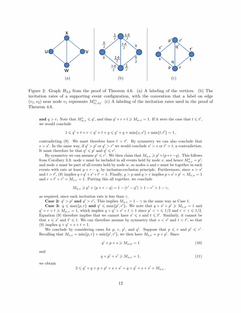
(a) (b) (c)

Figure 2: Graph H3,2 from the proof of Theorem 4.6. (a) A labeling of the vertices. (b) Theinvitation rates of a supporting event configuration, with the convention that a label on edge(v1, v2) near node v1 represents Mv1

v1,v2 . (c) A labeling of the invitation rates used in the proof ofTheorem 4.6.

and q > r. Note that Mxw,v 6 q′, and thus q′+ r+ t >Mw,v = 1. If it were the case that t 6 t′,

we would conclude

1 6 q′ + t+ r < q′ + t+ q 6 q′ + q + min{s, s′}+ min{t, t′} = 1 ,

contradicting (9). We must therefore have t > t′. By symmetry we can also conclude thats > s′. In the same way, if q′ > p′ or q′ > r′ we would conclude s′ > s or t′ > t, a contradiction.It must therefore be that q′ 6 p′ and q′ 6 r′.

By symmetry we can assume p′ 6 r′. We then claim that Mu,v > p′+(p+r−q). This followsfrom Corollary 3.3: node v must be included in all events held by node x, and hence Mx

u,v = p′;and node x must be part of all events held by node w, so nodes u and v must be together in suchevents with rate at least p + r − q, by inclusion-exclusion principle. Furthermore, since s > s′

and t > t′, (9) implies q+q′+s′+ t′ = 1. Finally, q > p and q > r implies p+s′+p′ = Mx,u = 1and r + t′ + r′ = Mx,v = 1. Putting this all together, we conclude

Mu,v > p′ + (p+ r − q) = 1− (r′ − q′) > 1− r′ > 1− γ,

as required, since each invitation rate is less than γ.Case 2: q′ > p′ and q′ > r′. This implies Mu,v > 1− γ in the same way as Case 1.Case 3: q 6 max{p, r} and q′ 6 max{p′, r′}. We note that q + s′ + p′ > Mx,u = 1 and

q′ + r + t > Mw,v = 1, which implies q + q′ + s′ + t > 1 since p′ < γ 6 1/2 and r < γ 6 1/2.Equation (9) therefore implies that we cannot have s′ 6 s and t 6 t′. Similarly, it cannot bethat s 6 s′ and t′ 6 t. We can therefore assume by symmetry that s < s′ and t < t′, so that(9) implies q + q′ + s+ t = 1.

We conclude by considering cases for p, r, p′, and q′. Suppose that p 6 r and p′ 6 r′.Recalling that Mu,v = min{p, r}+ min{p′, r′}, we then have Mu,v = p+ p′. Since

q′ + p+ s >Mu,w = 1 (10)

andq + p′ + s′ >Mu,x = 1, (11)

we obtain2 6 q′ + q + p+ p′ + s+ s′ = q + q′ + s+ s′ +Mu,v .

12

Combined with q+ q′+ s+ t = 1 and s′ < γ, it follows that Mu,v > 1−γ as required. The casesfor p > r and/or p′ > r′ are handled similarly, applying inequalities q′ + r + t > 1 in place of(10) and q + r′ + t′ > 1 in place of (11) as appropriate.

Proof of Theorem 4.10. Let n = |V | be the total community size. Write k? = b1/γc + 1.Split V into groups of k? agents and denote these groups by A1, . . . , Am, where m = n/k?. Nowtake i.i.d random subsets Xi ⊂ V of size K + 1− d1/γe from the community. Define

Yk =⋃i<k

{v ∈ Xk : v ∈ Xi, (Ak ∪ Yk) ∩Xi 6= ∅} and Zk = Xk \ Yk .

That is, the subsets Zi are similar to the subsets Xi, but “fixed” so that no pair of agents appearsin two different subsets. Now let each node in Ak invite Ak ∪ Zk (except itself) with rate γ.By our definition of Zk, the meeting rate for any two agents is either 0 or 1. This verifies thatthe configuration is stable. We now count the total degree D for the corresponding connectiongraph. Recalling that the meeting rate is either 0 or 1, we see D =

∑mk=1(|Zk|+k?−1)(|Zk|+k?).

Note that, by the union bound,

EYk 6 γmK + 1

n

(K + 1)2

n= o(1) .

This implies that with high probability, we have |k ∈ [n] : Yk > 1| = o(m). It then follows thatwith high probability

D > (1− o(1))mK(K + 1) = (1− o(1))nK(K + 1)/k? .

This guarantees the existence of a K-supportable graph with the required average degree.

References

[1] R. J. Aumann and R. B. Myerson. Endogenous formation of links between players and ofcoalitions: an application of the shapley value. In A. Roth, editor, In the shapley value.Cambridge University Press, 1998.

[2] V. Bala and S. Goyal. A noncooperative model of network formation. Econometrica, pages1181–1229, 2000.

[3] A.-L. Barabsi and R. Albert. Emergence of scaling in random networks. Science, pages509–512, 1999.

[4] F. Bloch and M. O. Jackson. The formation of networks with transfers among players.Journal of Economic Theory, 133(1):83–110, March 2007.

[5] B. Bollobas. Random graphs, volume 73 of Cambridge Studies in Advanced Mathematics.Cambridge University Press, Cambridge, second edition, 2001.

[6] B. Bollobas and O. Riordan. The diameter of a scale-free random graph. Combinatorica,24(1):5–34, 2004.

[7] B. Bollobas, O. Riordan, J. Spencer, and G. Tusnady. The degree sequence of a scale-freerandom graph process. Random Structures Algorithms, 18(3):279–290, 2001.

[8] S. A. Boorman. A combinatorial optimization model for transmission of job informationthrough contact networks. Bell Journal of Economics, 6(1):216–249, 1975.

[9] R. L. Breiger. The duality of persons and groups. Social Forces, 53(2):181–190, 1974.

[10] R. L. Breiger. Social control and social networks: A model from georg simmel. In C. Cal-houn, M. Meyer, and W. Scott, editors, Structures of power and constraint: papers in honorof Peter M. Blau, pages 453–476. Cambridge University Press, 1990.

13

[11] D. Easley and J. Kleinberg. Networks, Crowds, and Markets: Reasoning About a HighlyConnected World. Cambridge University Press, 2010.

[12] A. Fabrikant, E. Koutsoupias, and C. H. Papadimitriou. Heuristically optimized trade-offs:A new paradigm for power laws in the internet. In ICALP ’02: Proceedings of the 29thInternational Colloquium on Automata, Languages and Programming, 2002.

[13] A. Fabrikant, A. Luthra, E. Maneva, C. H. Papadimitriou, and S. Shenker. On a networkcreation game. In PODC ’03: Proceedings of the twenty-second annual symposium onPrinciples of distributed computing, 2003.

[14] S. Goyal. Connections: An introduction to the economics of networks. Princeton UniversityPress, 2007.

[15] M. O. Jackson. Social and Economic Networks. Princeton University Press, 2008.

[16] M. O. Jackson and B. W. Rogers. The economics of small worlds. Game theory andinformation, EconWPA, Mar. 2005.

[17] M. O. Jackson and A. Wolinsky. A strategic model of social and economic networks. InCMSEMS Discussion Paper 1098, Northwestern University, revised, 1995.

[18] R. Kumar, P. Raghavan, S. Rajagopalan, D. Sivakumar, A. Tomkins, and E. Upfal. Stochas-tic models for the web graph. In FOCS ’00: Proceedings of the 41st Annual Symposium onFoundations of Computer Science, 2000.

[19] S. Lattanzi and D. Sivakumar. Affiliation networks. In STOC ’09: Proceedings of the 41stannual ACM symposium on Theory of computing, pages 427–434, 2009.

[20] J. McPherson. Hypernetwork sampling: Duality and differentiation among voluntary or-ganizations. Social Networks, 3:225–249, 1982.

[21] M. Molloy and B. Reed. A critical point for random graphs with a given degree sequence.In Proceedings of the Sixth International Seminar on Random Graphs and ProbabilisticMethods in Combinatorics and Computer Science, “Random Graphs ’93” (Poznan, 1993).

[22] R. B. Myerson. Game theory: Analysis of conflict. Harvard Univ. Press, 1991.

[23] S. Wasserman and K. Faust. Canonical analysis of the composition and structure of socialnetworks. In C. Clogg, editor, Sociological Methodology, pages 142),, 1989.

14