1

The Hierarchical Structure of the Firm: A Geometric Perspective

Leopoldo Yanesa,*, Kam Ki Tanga

a School of Economics, University of Queensland, QLD, 4072, Australia

Abstract

This paper incorporates hierarchical structure into the neoclassical theory of the firm. Firms

are hierarchical in two respects: the organization of workers in production and the wage

structure. The firm’s hierarchy is represented as a sector of a circle, where the radius

represents the hierarchy’s height, the width of the sector represents the breadth of the

hierarchy at a given height, and the angle of the sector represents span of control. A perfectly

competitive firm chooses height and width, as well as capital, in order to maximize profit. We

analyze the short run and long run impact of changes in scale economies, input

substitutability, and input and output prices on the firm’s hierarchical structure. We find that

the firm grows as the specialization of its workers increases or as its output price increases

relative to input prices. The effect of changes in scale economies is contingent on the price of

output. The model also brings forth an analysis of wage inequality within the firm, which is

found to be independent of the firm’s hierarchical organization of workers, and only depends

on the firm’s wage schedule.

JEL classification: L22; L23; D63

Keywords: Theory of the firm; Hierarchical structure; Economies of scale; Input

substitutability; Inequality

* Corresponding author. Tel.: +617 3365 6619; fax: +617 3365 7299. E-mail address: L.Yanes@uq.edu.au

2

“An able man […] collects around him subordinates of more than ordinary

zeal and ability; as his business increases they rise with him, they trust him

and he trusts them…” (Marshall, 1898, Book IV, Ch. XIII, pp. 393-394)

1. Introduction

The hierarchical structure of firms exhibits ample variation. Firms in heavy manufacturing

industries typically have tall hierarchies (e.g., General Electric). Conversely, firms in the

services industry, such as consulting firms, tend to be relatively flat and less hierarchical

(e.g., Ernst & Young). What are the economic factors that influence the hierarchical structure

of firms? How does the hierarchical structure respond to a change in these factors? How is

production related to hierarchical structure?

The neoclassical theory of the firm, as stated in Samuelson (1947), is silent in these

respects. Narrowly defined, the neoclassical firm chooses inputs in order to maximize profit,

taking prices and technology as given. Labour is usually treated as a homogeneous input,

earning a uniform wage inside the firm. This treatment of labour is in great contrast with two

stylized facts of firms: (1) firms have fewer workers at higher ranks; and (2) wages rise with

the rank of workers within the hierarchy. These observations imply that firm production

involves a hierarchical organization of workers, as well as a hierarchical scheme of wages.

This paper incorporates hierarchical structure, in terms of production and wages, into

the neoclassical theory of the firm. The extended framework inherits the key features of

neoclassical firms whilst providing an analysis of the firm’s hierarchical structure and how

this affects the production process. This has the advantage of retaining standard results from

the neoclassical framework, whilst developing new insights regarding hierarchical structure,

in a parsimonious model. Instead of taking the span of control and number of levels in the

hierarchy as exogenous, we specify production directly in terms of these hierarchical

attributes.

A novelty of the paper is the use of a geometric approach to pose the optimization

problem. More specifically, we model the shape of the hierarchy using a sector of a circle.

This allows us to employ the geometric formulae related to the sector of a circle in the

construction of the cost function, which keeps the analysis tractable. This geometric approach

captures the essential features of the firm’s decision process, within a remarkably simple

3

framework. The firm maximizes profit by choosing capital, the height of the hierarchy, and

its width at each level. The height of the hierarchy is given by the radius of the sector. The

width is encompassed by the angle of the sector, or ‘span of control’.

The framework sheds new light on the question of the boundaries of the firm and firm

size, originally posed by Coase (1937). By solving the firm’s hierarchical structure design

problem, we provide a new characterization of Coase’s original insight, namely, that the firm

expands until the marginal benefit of doing so is no longer greater than the marginal cost. A

striking feature is that this is obtained without any reference to transaction costs. We

distinguish between vertical and horizontal expansion of the firm. In our framework, this

corresponds to the decision on the firm’s height, and its width at each hierarchical level.1

In considering the hierarchical structure of the firm, we come across the notion that

different levels of the hierarchy command different wage rates. We incorporate this by

introducing a wage schedule, which rises convexly with escalation along the hierarchy. This

brings forth the question of wage inequality within the firm. The simplicity of the framework

allows us to calculate Theil inequality indices (Theil, 1967) and to analyze how wage

inequality relates to the structure of the firm. By choosing a plausible parameterization for the

wage schedule, we obtain a measure of within firm wage inequality that approximates

observed earnings inequality in the United States.

1.1. Related Literature

With prescient insight, Marshall (1898, Book IV, Ch. XIII and 1923, Book II, Chs. X-XII)

noted the importance of hierarchical organization for the firm’s production process. More

recently, Erich Gutenberg (1951) argues that firm productivity depends on the organization

and complementarity of inputs rather than just the potential productivity of each input

(Albach et al., 2000). Other authors2 have also pointed out that the organization of workers,

when combined with other factors, influences how successful a firm is in achieving its

objective. The argument is that characteristics such as teamwork and the monitoring of

workers are crucial to the workings of the firm (Alchian and Demsetz, 1972).

Approaches to the hierarchical structure of the firm are diverse. One approach studies

the ‘distribution of authority’ within the firm. This approach attempts to explain how workers

1 One approach to the boundaries of the firm question is to consider firm scope (Teece, 1980) and vertical or lateral integration (Grossman and Hart, 1986). Alternatively, the problem can be viewed from the perspective of inputs, and the boundaries of the firm are then assessed in terms of its hierarchical structure (Wernerfelt, 1997). 2 Reviews of the literature can be found in Holmström and Tirole (1988) and Garrouste and Saussier (2005).

4

are organized according to the influence one has over others (Shapley and Palamara, 2000;

Rajan and Zingales, 2001; Hu and Shapley, 2003a, 2003b).

Another approach focuses on the ‘shape’ of the firm, and provides insights on its

structural design. The shape is determined by the number of levels in the hierarchy and by the

span of control of superiors. The models in this branch range from theories of knowledge

acquisition and communication flows (Garicano, 2000), information processing (Radner,

1992), promotion tournaments (Lazear and Rosen, 1981; Dubey and Haimanko, 2003), to

loss-of-control along the hierarchy, possibly due to imperfect communication (Williamson,

1967) or to imperfect observation and agency problems (Qian, 1994).

Other approaches deal with issues of asset ownership and control (Grossman and

Hart, 1986; Hart and Moore, 2005), as well as incentive (agency) problems (Jensen and

Meckling, 1976; Mookherjee and Reichelstein, 2001). In Yanes et al. (2005), we introduced a

geometric approach to the firm’s hierarchical design problem, focusing on a specific

example. The present study presents a more comprehensive treatment of that approach.

1.2. Structure of the Paper

In section 2, the firm’s general problem of hierarchical design is presented, and we show how

previous studies have reduced the general case to specific but tractable problems. Section 3

presents a model to solve a stylized version of the general problem. Section 4 offers an

illustration using specific functional forms. Section 5 then provides comparative statics

results for a particularly simple version of the model. Section 6 discusses wage inequality

within the firm. Conclusions are offered in section 7.

2. The General Problem

One can imagine a perfectly competitive firm that designs itself in order to maximise profit.

Its design problem is to choose how much labour and non-labour input to use, as well as how

to allocate its workers into different ‘positions’. Positions are defined by seniority and type of

activity (e.g., accounting, marketing, maintenance, etc), and each position is filled by one

worker. In solving this problem, a perfectly competitive firm takes output and input prices, as

well as technology, as given. In particular, the firm takes as given the market-determined

wage profile for workers being hired in different positions. On the other hand, the firm

determines the span of control of each worker, namely, how many supervisees he or she will

be responsible for. This is a difficult problem to solve, which can be stated formally in the

following manner. Let:

5

Price of output.Output.Price of non labour input.Non labour input.,..., denotes activity. Not all activities are performed in all hierarchical levels.,..., denotes level of seniority,

PYr

Ka 1 Ah 1 H

======

[ ]

with 1 being the highest.Number of supervisees for a worker at position .

, a matrix listing the supervision structure of the firm, i.e., span of control. Market wage rate for a wor

ah

ah A H

ah

ah

w

θθ

×

=

=

=

θker specialized in position .ah

The wage rate is typically rising with seniority. That is, is decreasing in h and can be

interpreted as a pay scale resulting from labour market conditions. The wage will also vary

between activities, but for our purposes this does not need to be specified. The firm’s

problem is specified as follows:

ahw

(1) ( ), , , s.t. , , , .max A H

ahA H Ka 1 h 1

PY w rK Y F A H K Y 0π= =

= − − ≤ ≥∑∑θ θ

( ), , ,F A H Kθ is the firm’s production technology. If F(.) is continuous and quasi-concave

(strictly or otherwise), then existence of solutions to the firm’s problem is warranted.

Moreover, if we impose strict quasi-concavity on F(.), or strict convexity on w(.), the solution

is unique. The production technology encompasses the details of how workers interact,

problems of monitoring, the efficiency of information and communication flows, and so

forth.

At this level of generality, the firm is free to choose any organizational form. We can

imagine pyramidal firms, with a single top manager. In this case there would be exactly one

worker at seniority level 1. Other structures are also possible. We can imagine a corporation

which is managed by a board of trustees. In this case, we could have several positions at

seniority level 1. Moreover, the organization need not necessarily expand (it may even

contract) as we move onto lower levels of seniority, and we can imagine positions which do

not have supervisory responsibilities, that is, they have no ‘off-spring’. Furthermore, the

optimal organizational structure need not be symmetric3. The resulting optimal structure will

depend on how A, H and affect output and costs, and the usual ‘marginal benefit equals

marginal cost’ reasoning applies.

θ

3 This framework could also be used to analyse not-for-profit organizations, e.g., charities, or some religious and governmental organizations. In this case profit maximization could be replaced with other objectives, such as output maximization subject to non-negative profits.

6

Several attempts have been made at solving problems of this type. Each approach

makes different simplifying assumptions in order to restore tractability. The closest papers to

our work are those by Williamson (1967) and Qian (1994), so we shall show how their

frameworks relate to the ‘general problem’ in (1). Both Qian and Williamson assume ‘no

working foremen’, that is, the only workers producing physical output are workers at the

bottom of the hierarchy. The contribution of higher level workers lies in inducing bottom

level workers to produce more, through coordination, monitoring, etc.

Williamson (1967) assumes that the span of control or the number of supervisees

( ahθ ) is constant across the hierarchy, wages increase with seniority at a constant rate, and

output is a Cobb-Douglas production function with the number of workers in each

hierarchical layer acting as inputs. In our notation, Williamson’s production function can be

written as ( ),

H 1 A

a hh 1 a 1Y c α θ

−

= == ∏ ∑ , where c is a constant converting input to output, and

( , )0 1α ∈ is a constant measuring loss of control. In this formulation the top manager’s

labour input is equal to unity, and bottom level workers do not have any supervisory duties.

Control loss is justified by reference to imperfect communication of instructions between

layers. With the exception of top management, control loss is present at all levels of the

hierarchy, and reduces the productivity of inputs, namely, the number of workers in each

hierarchical layer. With a constant span of control, the production function simplifies to

( )H 1Y c Aα θ −= (c.f., Williamson, 1967, p. 128). Williamson further assumes that non-labour

costs are a constant fraction of output. In this model, the only choice variable is the number

of layers in the hierarchy, which is chosen in order to maximize profit. The firm operates

under decreasing returns to scale, which arise from the loss-of-control problem.

Qian (1994) further elaborates Williamson’s approach by using optimal control

techniques to endogenize, in addition to number of layers in the hierarchy, the span of

control, loss of control and the shape of the wage schedule. Loss of control is now justified

by reference to misaligned incentives, and the firm solves a principal-agent problem which

results in workers receiving efficiency wages. Moreover, Qian allows for non-constant spans

of control, effort levels, and rates of increase for wages in the hierarchy. Assuming a fixed

capital-labour ratio, Qian specifies production as a recursive technology taking the

form h h 1y y hα−= , where denotes intermediate output at hierarchical level h-1 and h 1y −

[ ],h 0 1α ∈ denotes workers’ effort at hierarchical level h. Workers’ ability to choose effort is

the source of control loss. In our notation, final output can be written as follows:

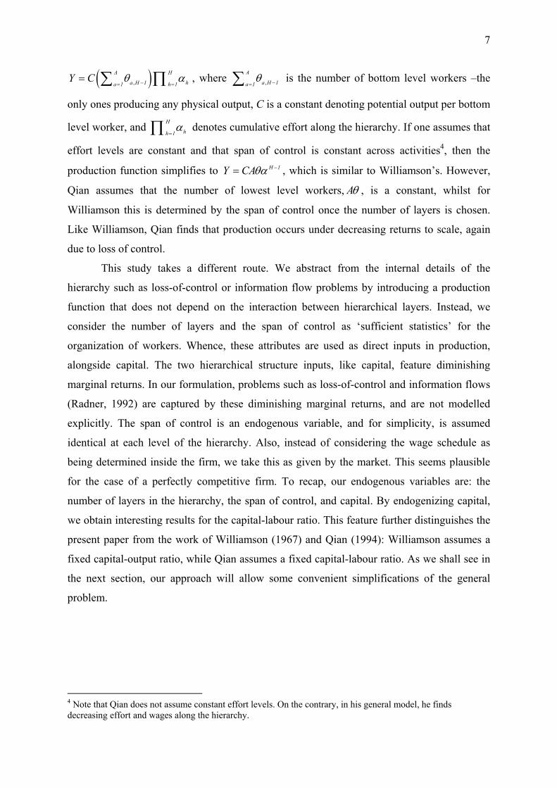
7

( ),

A

a H 1 ha 1 h 1Y C H

θ α−== ∑ ∏ =

, where ,

A

a H 1a 1θ −=∑ is the number of bottom level workers –the

only ones producing any physical output, C is a constant denoting potential output per bottom

level worker, and H

hh 1α

=∏ denotes cumulative effort along the hierarchy. If one assumes that

effort levels are constant and that span of control is constant across activities4, then the

production function simplifies to H 1Y CAθα −= , which is similar to Williamson’s. However,

Qian assumes that the number of lowest level workers, Aθ , is a constant, whilst for

Williamson this is determined by the span of control once the number of layers is chosen.

Like Williamson, Qian finds that production occurs under decreasing returns to scale, again

due to loss of control.

This study takes a different route. We abstract from the internal details of the

hierarchy such as loss-of-control or information flow problems by introducing a production

function that does not depend on the interaction between hierarchical layers. Instead, we

consider the number of layers and the span of control as ‘sufficient statistics’ for the

organization of workers. Whence, these attributes are used as direct inputs in production,

alongside capital. The two hierarchical structure inputs, like capital, feature diminishing

marginal returns. In our formulation, problems such as loss-of-control and information flows

(Radner, 1992) are captured by these diminishing marginal returns, and are not modelled

explicitly. The span of control is an endogenous variable, and for simplicity, is assumed

identical at each level of the hierarchy. Also, instead of considering the wage schedule as

being determined inside the firm, we take this as given by the market. This seems plausible

for the case of a perfectly competitive firm. To recap, our endogenous variables are: the

number of layers in the hierarchy, the span of control, and capital. By endogenizing capital,

we obtain interesting results for the capital-labour ratio. This feature further distinguishes the

present paper from the work of Williamson (1967) and Qian (1994): Williamson assumes a

fixed capital-output ratio, while Qian assumes a fixed capital-labour ratio. As we shall see in

the next section, our approach will allow some convenient simplifications of the general

problem.

4 Note that Qian does not assume constant effort levels. On the contrary, in his general model, he finds decreasing effort and wages along the hierarchy.

8

3. A Geometric Approach

Consider a sector of a circle as an abstract representation of the hierarchical structure of a

firm, as depicted in Figure 1. The height of the firm is represented by H, and can be

interpreted as the number of levels in the hierarchy. The angle, θ, can be interpreted as span

of control from any supervisor’s perspective: It measures the rate of expansion of the

workforce from one hierarchical layer to the next. In the figure, h represents the distance

from the highest position of the hierarchy. Thus h is inversely related to seniority, with h = 0

representing the top manager and h = H representing the lowest echelon of the hierarchy. b

represents the number of workers in a particular hierarchical level, h, and it can be interpreted

as the width of the firm at that level. Using the arc length formula, we have b = hθ.

b

h H θ

Figure 1. Firm Hierarchy as a Sector of a Circle

With this abstract representation, the problem of designing the hierarchical structure of the

firm is reduced to choosing the height (H) and the angle (θ ) of the sector. Similarly to

Williamson (1967) and Qian (1994), our representation does not deal with the question of

which activities are performed by which workers. As a result, the wage rate and output do not

depend on activities.

In posing the firm’s design problem as one of choosing the dimensions of a geometric

sector, we make the assumption that the hierarchy features a continuum of workers, both

horizontally and vertically. Thus, the area of the sector, given by , represents the

firm’s workforce. The firm’s profit is specified as follows:

2 / 2Hθ

(2) ( , ) ( ) ,H

0PY b h w h dh rKπ θ= − −∫

where P is output price, Y is output, r is the rental rate of capital, K is capital input,

( , )b h hθ θ= is the width of the hierarchy at level h, and is the wage schedule. The ( )w h

9

wage schedule is a differentiable, convex and decreasing function of h: ,

where subscripts denote first and second derivatives, respectively. We assume that this wage

schedule is set by the market. The firm is perfectly competitive, and consequently takes

prices, including the wage schedule, as given.

( ) 0, ( ) 0h hhw h w h< >

5

Hierarchical structure is incorporated directly into the firm’s production function,

allowing an inspection of the forces that affect hierarchical structure and production. The

major departure of our model from the standard neoclassical model of the firm is that the

labour input is measured in terms of H and θ, which enter the production function in the

following manner: ( , , )Y F H Kθ= . Since costs are strictly convex, all that is required for

existence and uniqueness of the solution to the firm’s profit maximization problem is that the

production function be continuous and strictly quasiconcave (for existence, but not

necessarily uniqueness, continuity and non-strict quasiconcavity are sufficient). In addition, it

will be convenient to assume that F(.) is twice continuously differentiable (C2), and features

diminishing marginal returns. Diminishing marginal returns to H and θ reflects the ‘loss-of-

control’ the top manager faces in the trade-off between height (distance to supervisees) and

width (span of control) of the hierarchy (Qian, 1994).

In the short run, capital is fixed and we introduce the following inequality

constraint: K K≤ . If we further assume that F(.) is increasing in its arguments, this constraint

will be binding. In this case, first order conditions for the firm’s optimization problem are

given by:

( ) ( )

( ) ( )

*H* *

0

* * * * *H

PF H , ,K hw h dh,

PF H , ,K H w H .

θ θ

θ θ

=

=

∫ (3)

If F(.) is strictly quasiconcave and C2, these yield unique solutions of the generic form *( , )P Kθ and *( , )H P K . The interpretation of (3) is straightforward; the left hand sides are

the marginal benefits from a marginal change in θ or H, respectively, and the right hand sides

are the marginal costs.

5 An interesting extension would be to endogenize the construction of the wage schedule. Qian (1994) obtains a convex and decreasing schedule based on the notion of imperfect observability of subordinates’ effort. To ameliorate the agency problem, Qian introduces efficiency wages and obtains a wage schedule which decreases along the hierarchy. An alternative route would be to consider the demand and supply sides of the labour market, together with some notion of differentiation in the labour input (perhaps drawing on differences in human capital). This extension lies outside the scope of this study, and its consideration is deferred for future work.

10

In the long run, capital is flexible and an additional first order condition needs to be

considered:

( )** ** **, ,KPF H K rθ .= (4)

Replacing K with in (3), equations (3)-(4) yield unique solutions of the following

generic form

**K6: ** ( , )P rθ , ** ( , )H P r , and ** ( , )K P r . Note that these factor demands do not

depend on wages. This is due to the fact that the wage schedule, , is determined once the

height of the hierarchy, H, has been chosen.

( )w h

4. An Illustrative Example

In this section we assume a specific functional form for the production function, ( , , )F H Kθ :

( ) /,Y K H

β ρα ρ ρθ= + (5)

with ρ < 1, ρ ≠ 0, α, β > 0. This implies that output depends not only on capital and labour,

but also on how the firm’s workforce is organized. Whereas the firm’s (unorganized)

workforce is equal to the area of the sector, given by , its ‘effective’ (organized)

labour is given by (

2 / 2Hθ

) /H

β ρρ ρθ+ .

4.1. Returns to Scale

If both θ and H change by factor , 1/3s s +∈ , the firm’s workforce becomes , while

effective labour changes to

2 / 2s Hθ

/ 3 /(s H )β ρ ρ βθ+ ρ . Thus, / 3β measures returns to scale in the

formation of effective labour, where:

(6) 1: decreasing returns to scale

/ 3 = 1: constant returns to scale1 : increasing returns to scale

β<⎧

⎪⎨⎪>⎩

To examine returns to scale in production of output, both the workforce and capital must

change by the same proportion, s. This is achieved by multiplying H and θ by and K by

s, yielding a new output of , where F(.) is as defined in (5). Thus,

1/3s/ 3 ( , , )s F H Kα β θ+ / 3α β+

measures returns to scale in production of output, where:

6 At this level of generality it is difficult to derive interesting comparative statics results, and in subsequent sections we shall make some simplifying assumptions to this end. The general results are available from the authors.

11

(7) 1: decreasing returns to scale

/ 3 = 1: constant returns to scale1 : increasing returns to scale

α β<⎧

⎪+ ⎨⎪>⎩

4.2. Elasticity of Substitution

In (5), the elasticity of substitution between H and θ is given by 1/(1-ρ). If workers at

different levels perform different tasks, then an increase in ρ indicates a decrease in the task

specialization of workers within the firm. In other words, there is a decrease in intra-firm

specialization. An indicator of intra-firm specialization is whether subordinates are able to fill

their superior’s role in case of absence, and vice versa. For example, intra-firm specialization

is expected to be higher in the manufacturing sector, relative to the fast food catering sector.

In a fast food shop, a manager can easily take up the task of cooking in the absence of some

workers. On the contrary, in a manufacturing factory, a manager may not be able to perform

the task of a technician. In particular, as H and θ become more substitutable, the firm would

be more inclined to give up one superior for another lower-level worker in order to reduce

total labour cost.

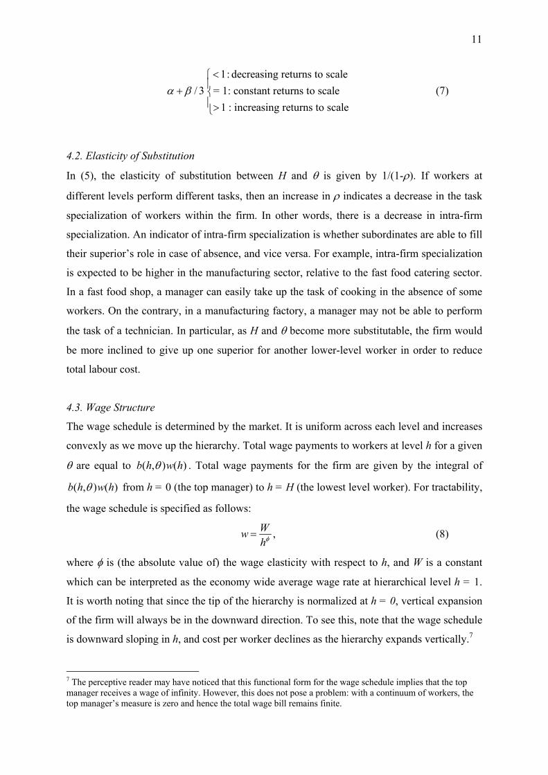
4.3. Wage Structure

The wage schedule is determined by the market. It is uniform across each level and increases

convexly as we move up the hierarchy. Total wage payments to workers at level h for a given

θ are equal to ( , ) ( )b h w hθ . Total wage payments for the firm are given by the integral of

( , ) ( )b h w hθ from h = 0 (the top manager) to h = H (the lowest level worker). For tractability,

the wage schedule is specified as follows:

,Wwhφ= (8)

where φ is (the absolute value of) the wage elasticity with respect to h, and W is a constant

which can be interpreted as the economy wide average wage rate at hierarchical level h = 1.

It is worth noting that since the tip of the hierarchy is normalized at h = 0, vertical expansion

of the firm will always be in the downward direction. To see this, note that the wage schedule

is downward sloping in h, and cost per worker declines as the hierarchy expands vertically.7

7 The perceptive reader may have noticed that this functional form for the wage schedule implies that the top manager receives a wage of infinity. However, this does not pose a problem: with a continuum of workers, the top manager’s measure is zero and hence the total wage bill remains finite.

12

In the short run, capital is fixed at K , thus, we need to consider only the distribution

and quantity of labour within the hierarchy. The firm’s problem is to choose H and θ in order

to maximize profit. After substituting the functional forms specified in (5) and (8), the

optimal values of H and θ solve the system set out in (3). This yields:

( )

( )2

13

*3

,2

PKW

β ρρ

φ ρρ

φ βα φβθ

φ

−

− −

− −⎡ ⎤−⎢= ⎢−⎢ ⎥⎣ ⎦

⎥⎥ (9)

( )( )

13

*1

3.

2

PKH W

β ρ φ βα ρ

β ρρ

φβ

φ

− − −

− −

⎡ ⎤−⎢= ⎢−⎢ ⎥⎣ ⎦

⎥⎥ (10)

To rule out complex values for θ * and H *, we assume φ < 2 in what follows. In the long run,

capital is no longer fixed but is chosen by the firm. To obtain the long run solutions, **θ , ,

and ; substitute (5) and (8) into (3) and (4), taking care to replace

**H**K K with in (3). The

solutions are as follows:

**K

( )

( )

1(1 ) (3 )(1 )

1**

(2 )(1 )1

3,

2P

r W

β ρ α φ α βρα α

ρ φ αα αρ

φα βθφ

− − − − −−

− − −−

⎡ ⎤−⎢= ⎢−⎢ ⎥⎣ ⎦

⎥⎥ (11)

( )

( )

1(1 ) (3 )(1 )

1**

(1 )(1 )1

3,

2H P

r W

β ρ α φ α βρα α

β ρ αα αρ

φα β

φ

− − − − −−

− + −−

⎡ ⎤−⎢= ⎢−⎢ ⎥⎣ ⎦

⎥⎥ (12)

( )( )

1(3 ) (3 )(1 )

3** 3

(2 )

3.

2K P r W

β ρ φ φ α βββ φ ρ

φβ ρ φ

ρ

φβα

φ

− − − − −− −

−− −

⎡ ⎤−⎛ ⎞⎢ ⎛ ⎞= ⎜ ⎟ ⎜ ⎟⎢ ⎝ ⎠ ⎝ ⎠ −⎢ ⎥⎣ ⎦

⎥⎥ (13)

We now proceed to make some simplifications in order to analyse these solutions.

5. Comparative Statics and Further Simplifications

In order to simplify the analysis of the comparative statics properties of the model, we set W

and φ to unity. This implies that the wage schedule, (8), is unit elastic. As will be shown later,

the choice of φ = 1 approximates the value of φ that matches the wage inequality implied by

the model with observed earnings inequality in the United States. These simplifications allow

13

a concise analysis of how the firm’s hierarchical structure responds to parameter changes. In

this simpler setting, the short run solutions in (9) and (10) simplify to

12

* * 2H PKβ ρ

.β

α ρθ β− −⎛ ⎞

= = ⎜⎝ ⎠

⎟ (14)

Similarly, the long run solutions in (11) - (13) simplify to

1(1 ) 2(1 )1

** ** 2H Pr

β ρ α

,α βα α

ρα

α βθ− − − −−⎡ ⎤

= = ⎢ ⎥⎣ ⎦

(15)

1(2 )2 2(1 )

** 2 2K P r

β ρβ

.α β

β ρα β−− − −⎡ ⎤⎛ ⎞= ⎜ ⎟⎢ ⎝ ⎠⎣ ⎦

⎥ (16)

As can be seen in (14) and (15), the simplification obtained by setting 1φ = introduces

symmetry into the firm’s hierarchical structure. It is important to acknowledge the limitation

that this imposes on the analysis, for such symmetry is unlikely to hold in reality.

Furthermore, setting W simplifies the second order conditions considerably. The

parsimony that these restrictions allow is such an attractive feature, that we decided to settle

for simplicity.

1=

Lemma 1. If W = φ = 1, second-order conditions for profit-maximization in the short run

require β < 2 and ρ < 0. In the long run, the requirements are α < 1, β < 2(1−α) and ρ < 0.

Proof: See the Appendix.

The upper bound of β implied by the long run second order conditions, β < 2(1−α), implies

that the firm operates under decreasing returns to scale. To see this, compare β < 2(1−α) with

/ 3α β+ < 1 from (7), to obtain β + 3α < β + 2α + 1 < 3, which implies diseconomies of

scale. This emerges because the wage is a decreasing function of h. Thus, the lowest rank

workers are paid progressively less as the firm expands its hierarchy. If workers’ productivity

did not fall at a sufficiently high rate as we move down the hierarchy, then a profit-

maximizing firm would expand indefinitely along the vertical dimension. To see the intuition

for restricting the substitutability between H and θ (ρ < 0), consider the case when H and θ

are perfectly substitutable ( 1ρ → ). In this case, the firm can save labour costs by

continuously expanding vertically and shrinking horizontally. In summary, β < 2(1−α) and

ρ < 0 ensure a firm of finite size.

14

The following propositions summarize the short run and long run comparative statics

properties of the simplified model:

Proposition 1. In the short run, the firm expands vertically and horizontally when output

price rises. In the long run, the firm expands vertically and horizontally, and deploys more

capital, when output price rises or the rental rate of capital falls.

Proof: In the short run, let * *Z H *θ= = . From Lemma 1, we have β < 2, hence:

*

*

1 02

P ZZ P β

∂= >

∂ −.

In the long run, let ** ** **Z H θ= = . From Lemma 1, we have β < 2(1−α), thus:

**

**

1 0,2(1 )

P ZZ P α β

∂= >

∂ − −

**

**

2 0,2(1 )

P KK P α β

∂= >

∂ − −

**

** 0,2(1 )

r ZZ r

αα β

∂ −= <

∂ − −

**

**

(2 ) 0.2(1 )

r KK r

βα β

∂ − −= <

∂ − −

As output price rises, marginal revenue rises and becomes greater than marginal cost. The

firm takes advantage of this by expanding its hierarchy8. In doing so, its marginal benefit

decreases while its marginal cost increases until they equate again. The result suggests that, in

industries in which output prices are protected (e.g., by regulation or trade barriers), firms

would be ‘bigger’ in terms of the number of workers they hire. Since 2(1−α)−β < 2−β,

changes in the hierarchical structure are greater in the long run than in the short run for a

given change in P. This is a specific instance of the Le Chatelier-Samuelson principle

(Samuelson, 1947).

Note also that the output price elasticity of **K is double that of **Z . Since the firm’s

workforce is equal to (area of the sector), the price elasticity of the firm’s workforce

is triple that of

2 / 2Hθ**Z . This means that if output price decreases, the firm’s labour force

contracts more than its capital stock in percentage terms, leading to an increase in the firm’s

capital-labour ratio. This is consistent with the observation that when firms face stronger

price competition in a deregulated environment, they typically respond by trimming the

workforce and streamlining production.

8 This result is also obtained by Williamson (1967) and Qian (1994), albeit using quite different frameworks.

15

In the short run the capital stock is fixed, so changes in the rental cost of capital have

no effect. However, in the long run, changes in the rental cost of capital affect the

hierarchical structure of the firm as well as the capital stock. The long run effects of a rise in

the rental cost of capital are of opposite sign to those of a rise in output price.

Proposition 2. In the short run, the firm’s hierarchy contracts horizontally and vertically as

intra-firm specialization decreases. In the long run, the firm’s hierarchy contracts

horizontally and vertically, and uses less capital, as intra-firm specialization decreases.

Proof: A decrease in intra-firm specialization is represented by an increase in substitutability

between H and θ (denoted by ρ). For the short run, using β < 2 and ρ < 0 (from Lemma 1),

we have:

*

* 21 ln 2 0.

(2 )

Z

Z

βρ ρ β

∂ −= <

∂ −

For the long run, using β < 2(1−α) and ρ <0 (from Lemma 1), we obtain: **

** 21 ln 2 0,

[2(1 ) ]

Z

Z

βρ ρ α β

∂ −= <

∂ − −

**

** 21 2 ln 2 0.

[2(1 ) ]

K

K

βρ ρ α β

∂ −= <

∂ − −

By Lemma 1, ρ is negative, hence an increase in ρ causes marginal revenue to decrease.

Therefore, the optimal response for the firm is to contract its hierarchy in order to cut costs

until marginal cost equates marginal revenue again. The result implies that firms would be

smaller (in terms of their labour force) in industries for which division of labour happens to a

lesser extent. This is consistent with the observation that a typical manufacturing firm is

greater in size than a typical service firm. An extreme example of the latter is the case of

tradespersons (‘one-man band’ firms), in which there is no division of labour, and the firm

attains the minimum size.

As before, the long run response of the firm’s hierarchical structure is greater than its

short run response. In the long run, a reduction in the firm’s workforce is accompanied by a

reduction in capital. As with output price, the elasticity of the firm’s workforce with respect

to ρ is 3/2 times that of capital. This means that as intra-firm specialization decreases, the

16

firm’s workforce falls more than capital in percentage terms, leading to an increase in the

firm’s capital-labour ratio.

Proposition 3. Provided output price is sufficiently high, an increase in returns to scale in

the formation of effective labour (that is, a rise in β) leads to an expansion of the hierarchy in

both the short run and long run, and an expansion of capital in the long run. Otherwise, it

leads to a contraction of the hierarchy in both the short and the long run, and a contraction

of capital in the long run.

Proof: In the short run, *

**

1 1 1 1 ln 2 ln(2 )

Z ZZ β β β ρ

⎛∂= + +⎜∂ − ⎝ ⎠

⎞⎟ . From Lemma 1, recall that

β < 2. If P is sufficiently large (such that *ln Z is sufficiently positive), then

*1 1 ln 2 ln 0,Zβ ρ

+ + >

which implies that . * / 0Z β∂ ∂ >

In the long run, **

****

1 1 1ln ln 2[2(1 ) ]

Z ZZ

αβ α β β ρ

⎛ ⎞∂ −= +⎜ ⎟∂ − − ⎝ ⎠

1+ , and

****

**

1 1 ln ln ln ln 1 (1 ) ln 2 /2(1 )

K K rK

α β ρβ α β

∂ ⎡ ⎤= + − + + + −⎣ ⎦∂ − −ρ . If P is sufficiently

large (such that **ln Z and **ln K are sufficiently positive), then

** 1 1ln ln 2 0,Z αβ ρ−

+ + > and (17)

(18) **ln ln ln ln 1 (1 )ln 2 / 0.K r α β ρ ρ+ − + + + − >

From Lemma 1, we have β < 2(1−α), which together with conditions (17) and (18) implies

and . ** /Z β∂ ∂ > 0 ** / 0K β∂ ∂ >

Conversely, if P is sufficiently low, it follows that * / 0Z β∂ ∂ < , and

.

** /Z β∂ ∂ < 0

0** /K β∂ ∂ <

A rise in β can be interpreted as an improvement in the ‘organizational technology’ of the

firm, that is, innovations in the way managers organize workers. Examples of this are

changes in the organizational structure of the firm, such as those implied by multidivisional

structure (M-form) versus the unitary structure (U-form). Maskin et al. (2000) explain how

17

the unitary form exploits scale/scope economies to a larger extent than the multidivisional

form. The results obtained in Proposition 3 imply that changes in returns to scale in the

formation of effective labour may not have a uniform effect on all firms. Rather, this will

depend on the firm’s environment. In a favourable environment with a high price for output,

an organizational innovation leads to firm expansion. Conversely, in an adverse setting, such

innovations lead to a contraction of the firm.

6. Wage Inequality within the Firm

In this section, we compute wage inequality with the firm, and show that for certain values of

φ, wage inequality will approximate the observed income inequality in the United States

during the 1980’s.

Income inequality is typically measured by the Gini coefficient, which involves pair

wise comparisons between individual incomes. Since our hierarchical firm features a

continuum of workers, pair wise comparisons are not meaningful. Instead, we measure

inequality using the Theil indices, which are members of the entropy family (Theil, 1967).

There are two Theil indices of inequality: Theil-L and Theil-T. In the discrete case,

the Theil-T measure of wage inequality within the firm is

0

( ) ( ) /ln( ) /

H

h

y h y h YY l h L=

⎛ ⎞= ⎜

⎝ ⎠∑T ⎟ (19)

where denotes wages earned by workers at hierarchical level h, with ( )y h ( ) ( )y h w h h hθ= ∆ ;

Y is the total wage bill of the firm, with ; is the total number of workers

between level h and level h+∆h, with

0( )

H

hY y h

=

= ∑ ( )l h

( )l h h hθ= ∆ ; and L is the firm’s workforce, with

. 0

( )H

hL l

=

= ∑ h

For the case when ( )w h Wh φ−= and 0h∆ → , (19) becomes

( )H 12 0

2 H2 h ln dhH 2

2ln .2 2

φφ

φ

φφ

φ φφ

−−

⎛ ⎞−−⎛ ⎞= ⎜ ⎟⎜ ⎟⎝ ⎠ ⎝

−⎛ ⎞= +⎜ ⎟ −⎝ ⎠

∫T⎠ (20)

Similarly, in the discrete case, the Theil-L measure of wage inequality within the firm is

0

( ) ( ) /ln ,( ) /

H

h

l h l h LL y h Y=

⎛= ⎜

⎝ ⎠∑L

⎞⎟ (21)

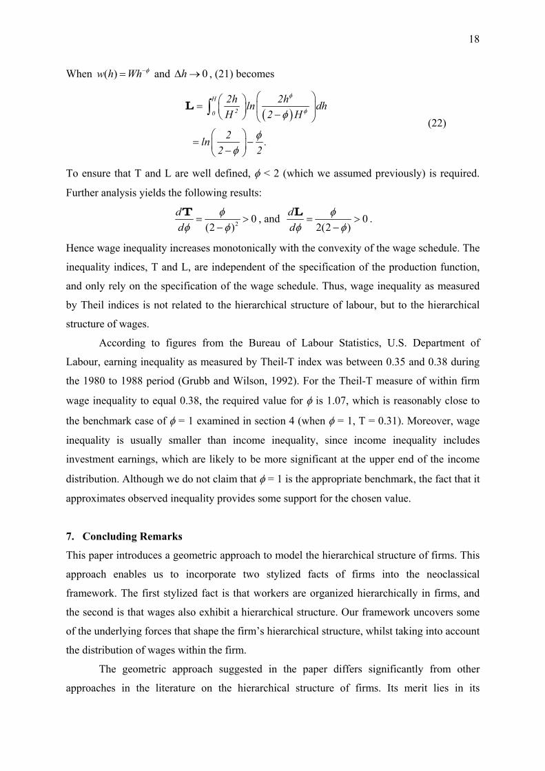
18

When ( )w h Wh φ−= and , (21) becomes 0h∆ →

( )

H

2 0

2h 2hln dhH 2 H

2ln .2 2

φ

φφ

φφ

⎛ ⎞⎛ ⎞= ⎜ ⎟⎜ ⎟ −⎝ ⎠ ⎝⎛ ⎞

= −⎜ ⎟−⎝ ⎠

∫L⎠ (22)

To ensure that T and L are well defined, φ < 2 (which we assumed previously) is required.

Further analysis yields the following results:

2 0(2 )

dd

φφ φ

= >−

T , and 02(2 )

dd

φφ φ

= >−

L .

Hence wage inequality increases monotonically with the convexity of the wage schedule. The

inequality indices, T and L, are independent of the specification of the production function,

and only rely on the specification of the wage schedule. Thus, wage inequality as measured

by Theil indices is not related to the hierarchical structure of labour, but to the hierarchical

structure of wages.

According to figures from the Bureau of Labour Statistics, U.S. Department of

Labour, earning inequality as measured by Theil-T index was between 0.35 and 0.38 during

the 1980 to 1988 period (Grubb and Wilson, 1992). For the Theil-T measure of within firm

wage inequality to equal 0.38, the required value for φ is 1.07, which is reasonably close to

the benchmark case of φ = 1 examined in section 4 (when φ = 1, T = 0.31). Moreover, wage

inequality is usually smaller than income inequality, since income inequality includes

investment earnings, which are likely to be more significant at the upper end of the income

distribution. Although we do not claim that φ = 1 is the appropriate benchmark, the fact that it

approximates observed inequality provides some support for the chosen value.

7. Concluding Remarks

This paper introduces a geometric approach to model the hierarchical structure of firms. This

approach enables us to incorporate two stylized facts of firms into the neoclassical

framework. The first stylized fact is that workers are organized hierarchically in firms, and

the second is that wages also exhibit a hierarchical structure. Our framework uncovers some

of the underlying forces that shape the firm’s hierarchical structure, whilst taking into account

the distribution of wages within the firm.

The geometric approach suggested in the paper differs significantly from other

approaches in the literature on the hierarchical structure of firms. Its merit lies in its

19

simplicity. With minor modifications on the standard neoclassical structure, the resulting

model sheds light on possible causes of variation in hierarchical structure.

By choosing specific functional forms for the production function and the wage

schedule, we obtain explicit short run and long run solutions for the firm’s optimal choice of

capital, hierarchical structure, and, as a result, labour. A simplified version of the model has

enabled us to examine how the firm’s hierarchical structure changes with output price, intra-

firm specialization, and technology (Propositions 1-3).

We have also shown that by choosing a plausible parameterization for the wage

schedule, the simplified model can generate an estimate of within-firm wage inequality that

approximates the observed earnings inequality in the United States.

The present framework also provides new answers to the questions of the boundaries

and size of the firm. The boundaries of the firm are now given by its height and width, and

the size of the firm (in terms of its labour force) is now given by the firm’s geometric shape.

The underlying forces behind these interpretations are of a similar spirit to Coase’s (1937)

original analysis, since the firm’s actions are guided by marginal considerations. However,

that is probably where any similarity ends, since the geometric approach itself is an entirely

novel framework. Moreover, the boundaries, size and shape of the firm are obtained without

any reference to transaction costs. Naturally, this is not to say that the latter are unimportant.

Rather, our message is that standard neoclassical forces, in particular returns to scale and

diminishing marginal returns, can be used to provide answers to the questions of the

boundaries, size, and shape of the firm. Transaction costs would then be an additional force,

the introduction of which serves to complement our analysis.

In the general problem outlined in section 2, a position in a firm is defined by two

attributes: the seniority of the position, and the activity performed in that position. This study,

like Qian (1994) and Williamson (1967), has not considered how activities affect a firm’s

hierarchical structure. For instance, the top manager may prefer to keep strategic activities at

arm’s length rather than delegating them to a ‘remote’ department. The role of activity in

designing hierarchical structure of firm remains unexplored, and we have only but raised the

question. The answers will have to wait for future research.

We close the discussion with a conjecture. Given the closeness of our approach to the

standard neoclassical paradigm, it should be possible to insert this model of the firm into a

general equilibrium framework. This would bring forth an analysis of the interaction between

economy-wide aspects, such as growth, trade and inequality on the one hand and the

hierarchical structure of firms on the other. This could be particularly useful in providing an

20

alternative approximation to the question posed by Qian (1994), on the differences between a

centrally planned economy featuring a single hierarchy and its capitalist counterpart featuring

a multitude of firms. This lies outside the scope of the present paper, and is deferred for

future work.

Appendix

Proof of Lemma 1:

In the short run, the firm’s profit simplifies to ( ) /

PK H H rKβ ρα ρ ρ

π θ θ= + − − . For *H

and *θ to be profit maximizing, the Hessian matrix must be negative semidefinite. The

Hessian is given by:

* *

* *,H

H HH

θθ θ

θ

π ππ π

⎛ ⎞= ⎜ ⎟

⎝ ⎠*H

where ‘*’ denotes values at the short-run optimum: H* and θ*, and subscripts denote second

order partial derivatives. Sufficient conditions for negative semidefiniteness of are as

follows:

*H

* * 0, 0HH θθπ π< < and * * *( )HH Hθθ θ2π π π> . Noting that and

, the sufficient conditions simplify to β < 2 and ρ <0.

* * ( 2HH θθ

β ρπ π= = + − ) / 2

/ 2* * ( 2)H Hθ θ

β ρπ π= = − −

In the long-run, the firm’s profit is ( )PK H H rKβ

α ρ ρ ρπ θ θ= + − − . The associated Hessian

is now

** ** **

** ** **

** ** **

,H K

H HH HK

K KH KK

θθ θ θ

θ

θ

π π ππ π ππ π π

⎛ ⎞⎜ ⎟= ⎜ ⎟⎜ ⎟⎝ ⎠

**H

where ** denotes values at the long-run optimum: K**, H** and θ **. Sufficient conditions for

negative semidefiniteness of are: **H ** 0iiπ < (i=K,H,θ), ** ** ** 2( )HH Hθθ θπ π π> , ** ** ** 2( )jj KK jKπ π π>

(for j=H,θ since ** **HH θθπ π= and ** **

HK Kθπ π= ), and 0<**H , where . denotes the

determinant. After simplification, sufficient conditions reduce to the following restrictions:

α< 1, β < 2(1−α) and ρ < 0.

21

Acknowledgement

We are grateful to Rodney Beard, Peter Davis, Peter Earl, Catherine de Fontenay, Evelyn Ng,

John Quiggin, and seminar participants at the University of Queensland and the Econometric

Society Meetings-Australasia for comments on earlier drafts. Rohan Alexander generously

provided ad-honorem research assistantship. Responsibility for any errors or shortcomings

remains with the authors.

References

Albach, H., Brockhoff, K., Eymann E., Jungen P., Steven, M., Luhmer, M., 2000. Theory of the Firm. Springer, Berlin and New York.

Alchian, A., Demsetz, H., 1972. Production, Information Costs, and Economic Organization. American Economic Review 62, 777–795.

Dubey, P., Haimanko, O., 2003. Optimal Scrutiny in Multi-period Promotion Tournaments. Games and Economic Behavior 42, 1-24.

Garicano, L., 2000. Hierarchies and the Organization of Knowledge in Production. Journal of Political Economy 108, 874-904.

Garrouste, P., Saussier, S., 2005. Looking for a Theory of the Firm: Future Challenges. Journal of Economic Behavior & Organization 58, 178-199.

Grossman, S., Hart, O., 1986. The Costs and Benefits of Ownership: A Theory of Vertical and Lateral Integration. Journal of Political Economy 94, 691-719.

Grubb, W., Wilson, R., 1992. Trends in Wage and Salary Inequality, 1967-88. Monthly Labour Review 115, 23-39.

Gutenberg, E., 1951/1971. Grundlagen der Betriebswirtschaftslehre, Vol I: Die Produktion. 1st edition/24th ed. Berlin, Heidelberg and New York: Springer-Verlag. Cited by Albach et al. 2000.

Hart, O., Moore, J., 2005. On the Design of Hierarchies: Coordination versus Specialization. Journal of Political Economy 113, 675-702.

Holmström, B., Tirole, J., 1988. The Theory of the Firm. In: Schmalensee, R., Willig, R., 1988. Handbook of Industrial Organization. North-Holland, Amsterdam.

Hu, X., Shapley, L., 2003a. On Authority Distributions in Organizations: Controls. Games and Economic Behavior 45, 153-170.

Hu, X., Shapley, L., 2003b. On Authority Distributions in Organizations: Equilibrium. Games and Economic Behavior 45, 132-152.

Jensen, M., Meckling, W., 1976. Theory of Firm-Managerial Behavior, Agency Costs and Ownership Structure. Journal of Financial Economics 3, 305-360.

Lazear, E., Rosen, S., 1981. Rank-Order Tournaments as Optimum Labor Contracts. Journal of Political Economy 89, 841-864.

Maskin, E., Qian, Y., Xu, C., 2000. Incentives, Information and Organizational Form. Review of Economic Studies 67, 359-378.

22

Marshall, A., 1898 Principles of Economics. 4th edition. MacMillan & Co., London.

Marshall, A., 1923. Industry and Trade: A Study of Industrial Technique and Business Organization; and of their Influences on the Conditions of Various Classes and Nations. 4th edition. MacMillan & Co., London.

Mookherjee, D., Reichelstein, S., 2001. Incentives and Coordination in Hierarchies. Advances in Theoretical Economics 1:1. Article 4. http://www.bepress.com/bejte/advances/vol1/iss1/art4.

Qian, Y., 1994. Incentives and Loss of Control in an Optimal Hierarchy. Review of Economic Studies 61, 527-544.

Radner, R., 1992. Hierarchy: The Economics of Managing. Journal of Economic Literature 30, 1382–1415.

Rajan, R., Zingales, L., 2001. The Firm as a Dedicated Hierarchy: A Theory of the Origins and Growth of Firms. Quarterly Journal of Economics 116, 805-851.

Samuelson, P., 1947. Foundations of Economic Analysis. Harvard University Press, Cambridge, Mass.

Samuelson, P., 1972. The Collected Scientific Papers of Paul A. Samuelson, Vol. 3 (edited by J. E. Stiglitz). M.I.T. Press, Cambridge, Mass.

Shapley, L., Palamara, J., 2000. Simple Games and Authority Structures. UCLA, mimeo.

Teece, D., 1980. Economies of Scope and the Scope of the Enterprise. Journal of Economic Behavior & Organization 1, 223-247.

Theil, H., 1967. Economics and Information Theory. North-Holland, Amsterdam.

Wernerfelt, B., 1997. On the Nature and Scope of the Firm: An Adjustment-cost Theory. Journal of Business 70, 489-514.

Williamson, O., 1967, Hierarchical Control and Optimum Firm Size. Journal of Political Economy 75, 123-138.

Yanes, L., Tang, K., Ng, E., Beard, R., 2005. The Hierarchical Structure of a Firm: A Geometric Approach. Economics Bulletin 12:13, 1−7, http://www.economicsbulletin.com/2005/volume12/EB−05L00004A.pdf