The HCI Stereo Metrics:Geometry-Aware Performance Analysis of Stereo Algorithms

Katrin Honauer1 Lena Maier-Hein2 Daniel Kondermann1

1HCI, Heidelberg Universityfirstname.lastname@iwr.uni-heidelberg.de

2German Cancer Research Center (DKFZ)l.maier-hein@dkfz-heidelberg.de

Abstract

Performance characterization of stereo methods ismandatory to decide which algorithm is useful for which ap-plication. Prevalent benchmarks mainly use the root meansquared error (RMS) with respect to ground truth disparitymaps to quantify algorithm performance.

We show that the RMS is of limited expressiveness foralgorithm selection and introduce the HCI Stereo Metrics.These metrics assess stereo results by harnessing three se-mantic cues: depth discontinuities, planar surfaces, andfine geometric structures. For each cue, we extract the rele-vant set of pixels from existing ground truth. We then applyour evaluation functions to quantify characteristics such asedge fattening and surface smoothness.

We demonstrate that our approach supports practition-ers in selecting the most suitable algorithm for their ap-plication. Using the new Middlebury dataset, we showthat rankings based on our metrics reveal specific algo-rithm strengths and weaknesses which are not quantified byexisting metrics. We finally show how stacked bar chartsand radar charts visually support multidimensional perfor-mance evaluation. An interactive stereo benchmark basedon the proposed metrics and visualizations is available at:http://hci.iwr.uni-heidelberg.de/stereometrics

1. Introduction

Disparity maps computed from stereo image pairs oftenserve as crucial input for higher level vision tasks such asobject detection, 3D reconstruction, and image based ren-dering, which are in turn used in applications such as driverassistance [31] and computer assisted surgery [24].

Fueled by the renowned Middlebury benchmark [34],stereo matching algorithms have made tremendous progressin the past decade. Since then, stereo benchmarks havebecome increasingly challenging, diverse and realisticwith datasets such as the new Middlebury dataset [33],

bes

t g

rou

nd

tru

th

seco

nd

th

ird

depth

discontinuities

A2

A3

A1

fine

structures

A1

A3

A2

planar

surfaces

A1

A3

A2

Figure 1: The same three algorithms A1-A3 rank differ-ently, depending on which of our proposed performancemetrics is used. For example, A1 is “the best algorithm”according to the widely used RMS measure. Yet, A1 yieldsthe lowest performance at depth discontinuities. The col-umn rankings show that our metrics allow for a more ex-pressive and semantically intuitive assessment of stereo re-sults with respect to depth discontinuities, planar surfaces,and fine structures. (Black denotes occluded regions.)

KITTI [10], HeiSt [20] and the new SINTEL stereo data [5].Top ranking algorithms on these benchmarks have long leftbehind purely pixel-based approaches. Instead, they hy-pothesize on local geometry, including segment-wise planefitting [16], explicit support for slanted and curved sur-faces [2, 39] as well as integrating sophisticated shape priorsand object recognition [3, 4, 12]. Even though this evolution

1

towards higher-level reasoning started more than ten yearsago, performance evaluation in the stereo community stillmainly works with purely pixelwise comparison of disparitydifferences. The two prevalent metrics are 1) RMS, whichdenotes the root mean squared pixelwise disparity differ-ence to a given ground truth disparity (GT) and 2) BadPix,the fraction of pixels whose disparity error exceeds a certainthreshold, commonly set to 1 or 2 pixels.

Given this situation, our goal is to let stereo evaluationcatch up with the progress of the stereo algorithms it is sup-posed to assess. Yet, introducing novel metrics for stereoevaluation is only justified if these metrics foster new valu-able insights and complement the established metrics RMSand BadPix. On the one hand, the established metrics al-ready fulfill many requirements for good performance met-rics as they are widely applicable, easy to compute, inde-pendent of image dimensions, and commonly accepted. Onthe other hand, metrics which average over all image pix-els cannot account for the fact that input pixels for stereoapplications are neither spatially independent nor equallyimportant or equally challenging.

In the Middlebury Stereo Evaluation v.31, Scharstein andHirschmuller address this issue by using binary masks foroccluded pixels and linear image weights for the overallranking. We build upon this idea and further flesh out theinformation given in existing GT disparity maps. We auto-matically extract GT pixel subsets of geometric structuresat semantically meaningful image regions such as planarsurfaces. These subsets can be extracted from differentGT datasets and applied to dense depth maps generated bystereo or other reconstruction methods.

Our contribution is threefold:

1. We propose the HCI Stereo Metrics, a novel set ofnine semantically intuitive metrics which characterizestereo performance at depth discontinuities, planar sur-faces, and fine structures (Section 3).

2. We re-evaluate recent Middlebury submissions, re-veal previously unquantified algorithm properties, anddemonstrate how metric combinations and multidi-mensional visualizations can be used to optimize forapplication-specific requirements (Section 4).

3. We provide source code for our evaluation frameworkand publish an interactive benchmarking website2.

2. Related WorkThe state-of-the-art performance evaluation method for

stereo algorithms clearly consists of comparing RMS scoresachieved on the Middlebury [33, 34] and KITTI [10]datasets with the published scores on the respective bench-mark websites. Both benchmarks provide scores computed

1http://vision.middlebury.edu/stereo/eval32http://hci.iwr.uni-heidelberg.de/stereometrics

on full, non-occluded and occluded pixel subsets. Middle-bury v.2 additionally provides scores for pixel subsets atdepth discontinuities.

Looking from a broader perspective, performance eval-uation for correspondence problems tends to be either verytheoretical or very application-specific [8, 19].

On the theoretical side, Barnard and Fischler defineda comprehensive set of characteristics ranging from ac-curacy and reliability to domain sensitivity and computa-tional complexity [1]. Maimone and Shafer analyzed whichperformance characteristics can be assessed on test setupsranging from empirical uncontrolled environments over en-gineered test data to pure mathematical analysis [25]. Har-alick suggested sound statistical performance characteriza-tion with random perturbations of the algorithm input [13].Despite their mathematical universality, most of these eval-uation methods are hardly feasible for stereo evaluation incurrent research and real-world scenarios because they of-ten require exact and comprehensive models of the algo-rithms, problem domains, and input data.

On the application-oriented side, a variety of evaluationmethods has been proposed, such as for pedestrian or lanedetection in driver assistance scenarios [9, 17, 27, 31].Maier-Hein et al. proposed evaluation metrics for stereoaccuracy, robustness, point density and computation time inlaparoscopic surgery [23, 24]. Further specialized evalua-tion methods were proposed with regard to immersive vi-sualization for tele-presence [29], video surveillance sys-tems [37], and imaging parameter dependence on Mars mis-sions [18]. Those methods accomplish their specific pur-pose very well but the problem-specific insights are oftennot easily transferable to other domains.

Our goal is to find a good trade-off between those twoareas of research. We aim at developing theoretically soundgeneral purpose metrics which are nonetheless easily appli-cable to existing benchmark datasets and parameterizable tosuit the specific needs of different applications.

In the stereo community, Kostkova et al. reasoned thatperformance evaluation should take the algorithm purposeinto account and showed that evaluation must not be lim-ited to basic pixel averaging [21]. Instead, they discriminatematching errors such as the false negative rate and occlu-sion boundary inaccuracy. Furthermore, we borrow ideasfrom the segmentation and object detection communities toinclude higher level reasoning about the image structure:Margolin et al. proposed evaluation metrics for foregroundmaps which incorporate the fact that pixels are neither spa-tially independent nor equally important [26]. Ozdemir etal. developed performance metrics for object detection eval-uation which are sensitive to boundary and fragmentationerrors [30]. Yasnoff et al. state that good metrics for scenesegmentation should incorporate error categories for differ-ent picture elements and have adjustable costs [38].

3. Novel Metrics for Stereo EvaluationIn this Section, we introduce theoretical principles for

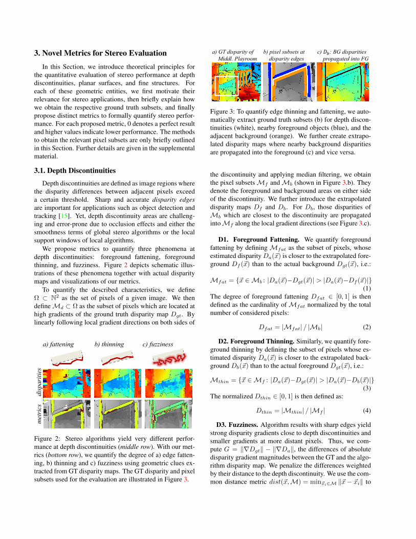
the quantitative evaluation of stereo performance at depthdiscontinuities, planar surfaces, and fine structures. Foreach of these geometric entities, we first motivate theirrelevance for stereo applications, then briefly explain howwe obtain the respective ground truth subsets, and finallypropose distinct metrics to formally quantify stereo perfor-mance. For each proposed metric, 0 denotes a perfect resultand higher values indicate lower performance. The methodsto obtain the relevant pixel subsets are only briefly outlinedin this Section. Further details are given in the supplementalmaterial.

3.1. Depth Discontinuities

Depth discontinuities are defined as image regions wherethe disparity differences between adjacent pixels exceeda certain threshold. Sharp and accurate disparity edgesare important for applications such as object detection andtracking [15]. Yet, depth discontinuity areas are challeng-ing and error-prone due to occlusion effects and either thesmoothness terms of global stereo algorithms or the localsupport windows of local algorithms.

We propose metrics to quantify three phenomena atdepth discontinuities: foreground fattening, foregroundthinning, and fuzziness. Figure 2 depicts schematic illus-trations of these phenomena together with actual disparitymaps and visualizations of our metrics.

To quantify the described characteristics, we defineΩ ⊂ N2 as the set of pixels of a given image. We thendefineMd ⊂ Ω as the subset of pixels which are located athigh gradients of the ground truth disparity map Dgt. Bylinearly following local gradient directions on both sides of

c) fuzziness a) fattening b) thinning

dis

pa

riti

es

met

rics

Figure 2: Stereo algorithms yield very different perfor-mance at depth discontinuities (middle row). With our met-rics (bottom row), we quantify the degree of a) edge fatten-ing, b) thinning and c) fuzziness using geometric clues ex-tracted from GT disparity maps. The GT disparity and pixelsubsets used for the evaluation are illustrated in Figure 3.

a) GT disparity of

Middl. Playroom

c) 𝐷𝑏: BG disparities

propagated into FG

b) pixel subsets at

disparity edges

Figure 3: To quantify edge thinning and fattening, we auto-matically extract ground truth subsets (b) for depth discon-tinuities (white), nearby foreground objects (blue), and theadjacent background (orange). We further create extrapo-lated disparity maps where nearby background disparitiesare propagated into the foreground (c) and vice versa.

the discontinuity and applying median filtering, we obtainthe pixel subsetsMf andMb (shown in Figure 3.b). Theydenote the foreground and background areas on either sideof the discontinuity. We further introduce the extrapolateddisparity maps Df and Db. For Db, those disparities ofMb which are closest to the discontinuity are propagatedintoMf along the local gradient directions (see Figure 3.c).

D1. Foreground Fattening. We quantify foregroundfattening by defining Mfat as the subset of pixels, whoseestimated disparity Da(~x) is closer to the extrapolated fore-ground Df (~x) than to the actual background Dgt(~x), i.e.:

Mfat = ~x ∈Mb : |Da(~x)−Dgt(~x)| > |Da(~x)−Df (~x)|(1)

The degree of foreground fattening Dfat ∈ [0, 1] is thendefined as the cardinality ofMfat normalized by the totalnumber of considered pixels:

Dfat = |Mfat| / |Mb| (2)

D2. Foreground Thinning. Similarly, we quantify fore-ground thinning by defining the subset of pixels whose es-timated disparity Da(~x) is closer to the extrapolated back-ground Db(~x) than to the actual foreground Dgt(~x), i.e.:

Mthin = ~x ∈Mf : |Da(~x)−Dgt(~x)| > |Da(~x)−Db(~x)|(3)

The normalized Dthin ∈ [0, 1] is then defined as:

Dthin = |Mthin| / |Mf | (4)

D3. Fuzziness. Algorithm results with sharp edges yieldstrong disparity gradients close to depth discontinuities andsmaller gradients at more distant pixels. Thus, we com-pute G = ‖∇Dgt‖ − ‖∇Da‖, the differences of absolutedisparity gradient magnitudes between the GT and the algo-rithm disparity map. We penalize the differences weightedby their distance to the depth discontinuity. We use the com-mon distance metric dist(~x,M) = min~xi∈M ‖~x− ~xi‖ to

find the closest element in the set of edge area pixelsMe =Md ∪Mf ∪Mb. Furthermore, we define:

f(~x) =

|G(~x)|·dist(~x,Md), if G(~x) < 0

G(~x) · dist(~x,Ω \Me), otherwise(5)

which penalizes overly strong gradients by their distance todiscontinuities and overly soft gradients by their closeness.Finally, we quantify the fuzziness of discontinuities as:

Dfuz =1

|Me|∑

~x∈Me

f(~x) (6)

3.2. Planar Surfaces

Reconstructed planar surfaces are used with very dif-ferent requirements among stereo applications like image-based rendering or driver assistance. While some applica-tions care about the correct principal orientation, others re-quire the exact distance or prefer smooth but slightly tiltedplanes over more accurate yet uneven planes with artifacts.

A common strategy among many stereo algorithms is tofit local planes or splines to some sort of superpixels [16,35, 39]. Their parametrization often is a trade-off betweenlocally accurate fits with jumps between the superpixels orsmoother yet less accurate results.

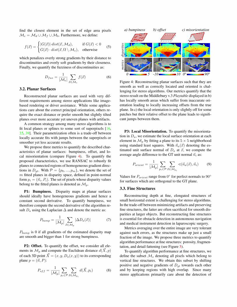
We propose three metrics to quantify the described char-acteristics of planar surfaces: bumpiness, offset, and lo-cal misorientation (compare Figure 4). To quantify theproposed characteristics, we use RANSAC to robustly fitplanes to connected regions of homogeneous gradient direc-tions in Dgt. With P = p0, ..., pm, we denote the set ofm fitted planes in disparity space, defined in point-normalform pi = (~ni, Pi). The set of pixels whose disparity valuesbelong to the fitted planes is denoted asMp.

P1: Bumpiness. Disparity maps at planar surfacesshould ideally have homogeneous gradients and hence aconstant second derivative. To quantify bumpiness, wetherefore compute the second derivative of the algorithm re-sult Da using the Laplacian ∆ and denote the metric as:

Pbump =1

|Mp|∑

~x∈Mp

|∆Da(~x)| (7)

Pbump is 0 if all gradients of the estimated disparity mapare smooth and bigger than 1 for strong bumpiness.

P2: Offset. To quantify the offset, we consider all ele-ments inMp and compute the Euclidean distance d( ~X, p)

of each 3D point ~X = (x, y,Da(x, y)) to its correspondingplane p = (~n, P ):

Poff =1

|Mp|∑pi∈P

∑~x∈Mpi

d( ~X, pi) (8)

10 -10 0 90° 0° 5

a) bumpiness b) offset c) misorientation

dis

pari

ties

m

etri

cs

Figure 4: Reconstructing planar surfaces such that they aresmooth as well as correctly located and oriented is chal-lenging for stereo algorithms. Our metrics quantify that thestereo result on the Middlebury v.3 Playtable displayed in b)has locally smooth areas which suffer from inaccurate ori-entation leading to locally increasing offsets from the trueplane. In c) the local orientation is only slightly off for somepatches but their relative offset to the plane leads to signifi-cant jumps between them.

P3: Local Misorientation. To quantify the misorienta-tion in Da, we estimate the local surface orientation at eachelement inMp by fitting a plane to its 5× 5 neighborhoodusing standard least squares. With ~na(~x) denoting the es-timated unit surface normal of Da at ~x, we compute theaverage angle difference to the GT unit normal ~ni as:

Porient =1

|Mp|∑pi∈P

∑~x∈Mpi

^(~na(~x), ~ni) (9)

Values for Porient range from 0 for perfect normals to 90

for surfaces which are orthogonal to the GT plane.

3.3. Fine Structures

Reconstructing depth at fine, elongated structures ofsmall horizontal extent is challenging for stereo algorithms.In the trade-off between minimizing artifacts and preservingfine structures, the latter are often sacrificed for smooth dis-parities at larger objects. But reconstructing fine structuresis essential for obstacle detection in autonomous navigationand medical instrument detection in laparoscopic surgery.

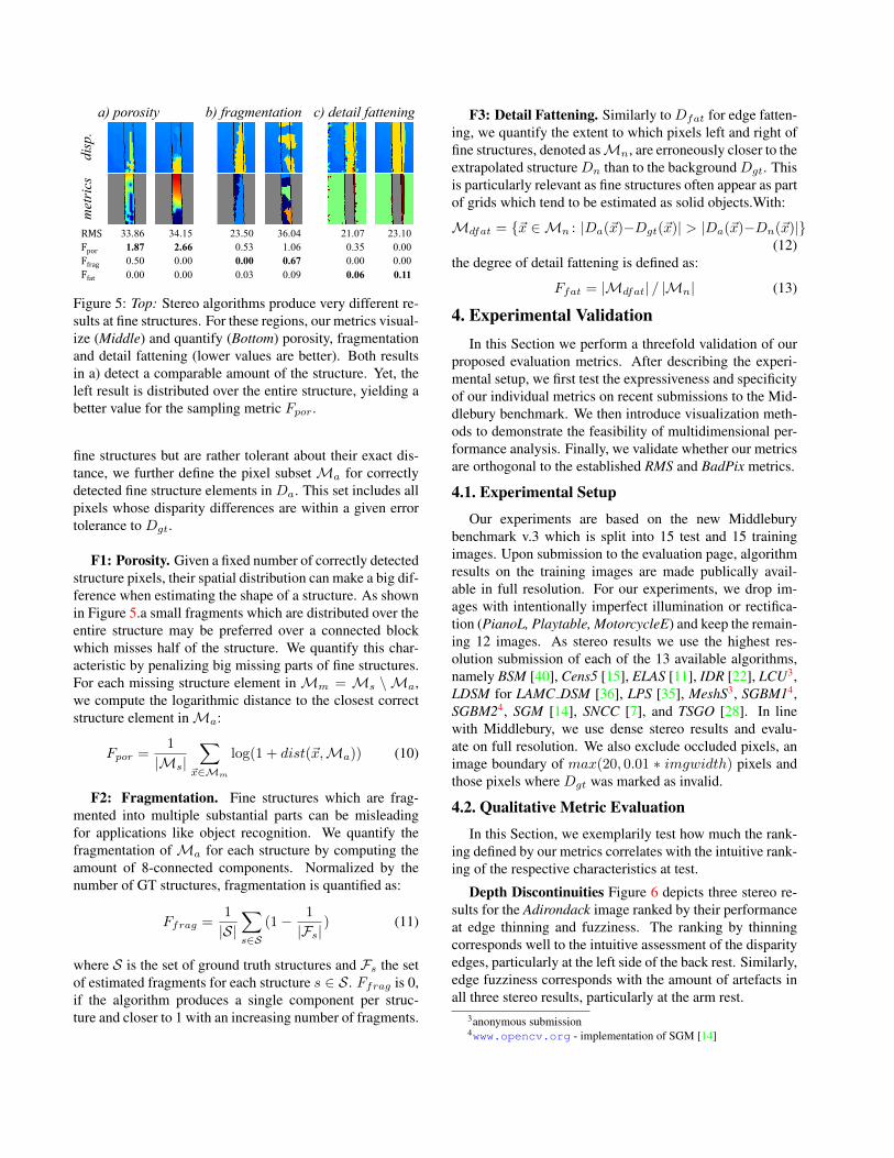
Metrics averaging over the entire image are very tolerantagainst such errors, as the structures make up just a smallfraction of the image. We propose three metrics to quantifyalgorithm performance at fine structures: porosity, fragmen-tation, and detail fattening (see Figure 5).

To quantify algorithm performance at fine structures, wedefine the subset Ms denoting all pixels which belong tovertical fine structures. We obtain this subset by shiftingpositive and negative gradients of Dgt towards each otherand by keeping regions with high overlap. Since manystereo applications primarily care about the detection of

a) porosity b) fragmentation c) detail fattening

dis

p.

met

rics

RMS 33.86 34.15 23.50 36.04 21.07 23.10

Fpor 1.87 2.66 0.53 1.06 0.35 0.00

Ffrag 0.50 0.00 0.00 0.67 0.00 0.00

Ffat 0.00 0.00 0.03 0.09 0.06 0.11

Figure 5: Top: Stereo algorithms produce very different re-sults at fine structures. For these regions, our metrics visual-ize (Middle) and quantify (Bottom) porosity, fragmentationand detail fattening (lower values are better). Both resultsin a) detect a comparable amount of the structure. Yet, theleft result is distributed over the entire structure, yielding abetter value for the sampling metric Fpor.

fine structures but are rather tolerant about their exact dis-tance, we further define the pixel subset Ma for correctlydetected fine structure elements in Da. This set includes allpixels whose disparity differences are within a given errortolerance to Dgt.

F1: Porosity. Given a fixed number of correctly detectedstructure pixels, their spatial distribution can make a big dif-ference when estimating the shape of a structure. As shownin Figure 5.a small fragments which are distributed over theentire structure may be preferred over a connected blockwhich misses half of the structure. We quantify this char-acteristic by penalizing big missing parts of fine structures.For each missing structure element inMm = Ms \ Ma,we compute the logarithmic distance to the closest correctstructure element inMa:

Fpor =1

|Ms|∑

~x∈Mm

log(1 + dist(~x,Ma)) (10)

F2: Fragmentation. Fine structures which are frag-mented into multiple substantial parts can be misleadingfor applications like object recognition. We quantify thefragmentation of Ma for each structure by computing theamount of 8-connected components. Normalized by thenumber of GT structures, fragmentation is quantified as:

Ffrag =1

|S|∑s∈S

(1− 1

|Fs|) (11)

where S is the set of ground truth structures and Fs the setof estimated fragments for each structure s ∈ S. Ffrag is 0,if the algorithm produces a single component per struc-ture and closer to 1 with an increasing number of fragments.

F3: Detail Fattening. Similarly to Dfat for edge fatten-ing, we quantify the extent to which pixels left and right offine structures, denoted asMn, are erroneously closer to theextrapolated structure Dn than to the background Dgt. Thisis particularly relevant as fine structures often appear as partof grids which tend to be estimated as solid objects.With:

Mdfat = ~x ∈Mn : |Da(~x)−Dgt(~x)| > |Da(~x)−Dn(~x)|(12)

the degree of detail fattening is defined as:

Ffat = |Mdfat| / |Mn| (13)

4. Experimental ValidationIn this Section we perform a threefold validation of our

proposed evaluation metrics. After describing the experi-mental setup, we first test the expressiveness and specificityof our individual metrics on recent submissions to the Mid-dlebury benchmark. We then introduce visualization meth-ods to demonstrate the feasibility of multidimensional per-formance analysis. Finally, we validate whether our metricsare orthogonal to the established RMS and BadPix metrics.

4.1. Experimental Setup

Our experiments are based on the new Middleburybenchmark v.3 which is split into 15 test and 15 trainingimages. Upon submission to the evaluation page, algorithmresults on the training images are made publically avail-able in full resolution. For our experiments, we drop im-ages with intentionally imperfect illumination or rectifica-tion (PianoL, Playtable, MotorcycleE) and keep the remain-ing 12 images. As stereo results we use the highest res-olution submission of each of the 13 available algorithms,namely BSM [40], Cens5 [15], ELAS [11], IDR [22], LCU3,LDSM for LAMC DSM [36], LPS [35], MeshS3, SGBM14,SGBM24, SGM [14], SNCC [7], and TSGO [28]. In linewith Middlebury, we use dense stereo results and evalu-ate on full resolution. We also exclude occluded pixels, animage boundary of max(20, 0.01 ∗ imgwidth) pixels andthose pixels where Dgt was marked as invalid.

4.2. Qualitative Metric Evaluation

In this Section, we exemplarily test how much the rank-ing defined by our metrics correlates with the intuitive rank-ing of the respective characteristics at test.

Depth Discontinuities Figure 6 depicts three stereo re-sults for the Adirondack image ranked by their performanceat edge thinning and fuzziness. The ranking by thinningcorresponds well to the intuitive assessment of the disparityedges, particularly at the left side of the back rest. Similarly,edge fuzziness corresponds with the amount of artefacts inall three stereo results, particularly at the arm rest.

3anonymous submission4www.opencv.org - implementation of SGM [14]

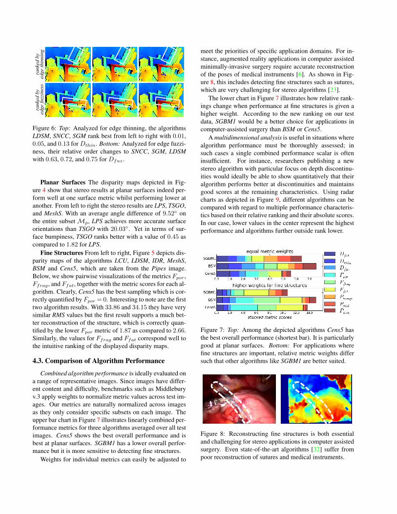
ranke

d b

y e

dge

fuzz

ines

s ra

nke

d b

y

edge

thin

nin

g

Figure 6: Top: Analyzed for edge thinning, the algorithmsLDSM, SNCC, SGM rank best from left to right with 0.01,0.05, and 0.13 for Dthin. Bottom: Analyzed for edge fuzzi-ness, their relative order changes to SNCC, SGM, LDSMwith 0.63, 0.72, and 0.75 for Dfuz .

Planar Surfaces The disparity maps depicted in Fig-ure 4 show that stereo results at planar surfaces indeed per-form well at one surface metric whilst performing lower atanother. From left to right the stereo results are LPS, TSGO,and MeshS. With an average angle difference of 9.52 onthe entire subsetMp, LPS achieves more accurate surfaceorientations than TSGO with 20.03. Yet in terms of sur-face bumpiness, TSGO ranks better with a value of 0.45 ascompared to 1.82 for LPS.

Fine Structures From left to right, Figure 5 depicts dis-parity maps of the algorithms LCU, LDSM, IDR, MeshS,BSM and Cens5, which are taken from the Pipes image.Below, we show pairwise visualizations of the metrics Fpor,Ffrag, and Ffat, together with the metric scores for each al-gorithm. Clearly, Cens5 has the best sampling which is cor-rectly quantified by Fpor = 0. Interesting to note are the firsttwo algorithm results. With 33.86 and 34.15 they have verysimilar RMS values but the first result supports a much bet-ter reconstruction of the structure, which is correctly quan-tified by the lower Fpor metric of 1.87 as compared to 2.66.Similarly, the values for Ffrag and Ffat correspond well tothe intuitive ranking of the displayed disparity maps.

4.3. Comparison of Algorithm Performance

Combined algorithm performance is ideally evaluated ona range of representative images. Since images have differ-ent content and difficulty, benchmarks such as Middleburyv.3 apply weights to normalize metric values across test im-ages. Our metrics are naturally normalized across imagesas they only consider specific subsets on each image. Theupper bar chart in Figure 7 illustrates linearly combined per-formance metrics for three algorithms averaged over all testimages. Cens5 shows the best overall performance and isbest at planar surfaces. SGBM1 has a lower overall perfor-mance but it is more sensitive to detecting fine structures.

Weights for individual metrics can easily be adjusted to

meet the priorities of specific application domains. For in-stance, augmented reality applications in computer assistedminimally-invasive surgery require accurate reconstructionof the poses of medical instruments [6]. As shown in Fig-ure 8, this includes detecting fine structures such as sutures,which are very challenging for stereo algorithms [23].

The lower chart in Figure 7 illustrates how relative rank-ings change when performance at fine structures is given ahigher weight. According to the new ranking on our testdata, SGBM1 would be a better choice for applications incomputer-assisted surgery than BSM or Cens5.

A multidimensional analysis is useful in situations wherealgorithm performance must be thoroughly assessed; insuch cases a single combined performance scalar is ofteninsufficient. For instance, researchers publishing a newstereo algorithm with particular focus on depth discontinu-ities would ideally be able to show quantitatively that theiralgorithm performs better at discontinuities and maintainsgood scores at the remaining characteristics. Using radarcharts as depicted in Figure 9, different algorithms can becompared with regard to multiple performance characteris-tics based on their relative ranking and their absolute scores.In our case, lower values in the center represent the highestperformance and algorithms further outside rank lower.

Figure 7: Top: Among the depicted algorithms Cens5 hasthe best overall performance (shortest bar). It is particularlygood at planar surfaces. Bottom: For applications wherefine structures are important, relative metric weights differsuch that other algorithms like SGBM1 are better suited.

Figure 8: Reconstructing fine structures is both essentialand challenging for stereo applications in computer assistedsurgery. Even state-of-the-art algorithms [32] suffer frompoor reconstruction of sutures and medical instruments.

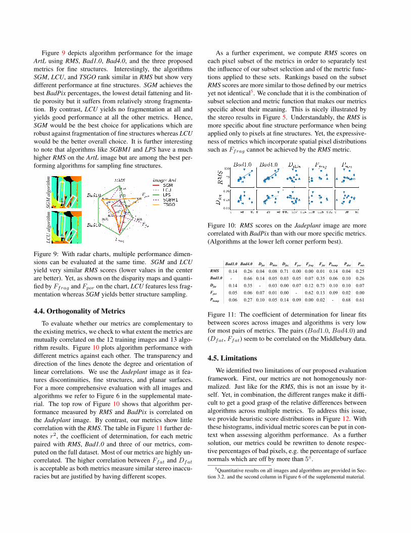
Figure 9 depicts algorithm performance for the imageArtL using RMS, Bad1.0, Bad4.0, and the three proposedmetrics for fine structures. Interestingly, the algorithmsSGM, LCU, and TSGO rank similar in RMS but show verydifferent performance at fine structures. SGM achieves thebest BadPix percentages, the lowest detail fattening and lit-tle porosity but it suffers from relatively strong fragmenta-tion. By contrast, LCU yields no fragmentation at all andyields good performance at all the other metrics. Hence,SGM would be the best choice for applications which arerobust against fragmentation of fine structures whereas LCUwould be the better overall choice. It is further interestingto note that algorithms like SGBM1 and LPS have a muchhigher RMS on the ArtL image but are among the best per-forming algorithms for sampling fine structures.

LC

U a

lgori

thm

SG

M a

lgori

thm

Figure 9: With radar charts, multiple performance dimen-sions can be evaluated at the same time. SGM and LCUyield very similar RMS scores (lower values in the centerare better). Yet, as shown on the disparity maps and quanti-fied by Ffrag and Fpor on the chart, LCU features less frag-mentation whereas SGM yields better structure sampling.

4.4. Orthogonality of Metrics

To evaluate whether our metrics are complementary tothe existing metrics, we check to what extent the metrics aremutually correlated on the 12 training images and 13 algo-rithm results. Figure 10 plots algorithm performance withdifferent metrics against each other. The transparency anddirection of the lines denote the degree and orientation oflinear correlations. We use the Jadeplant image as it fea-tures discontinuities, fine structures, and planar surfaces.For a more comprehensive evaluation with all images andalgorithms we refer to Figure 6 in the supplemental mate-rial. The top row of Figure 10 shows that algorithm per-formance measured by RMS and BadPix is correlated onthe Jadeplant image. By contrast, our metrics show littlecorrelation with the RMS. The table in Figure 11 further de-notes r2, the coefficient of determination, for each metricpaired with RMS, Bad1.0 and three of our metrics, com-puted on the full dataset. Most of our metrics are highly un-correlated. The higher correlation between Ffat and Dfat

is acceptable as both metrics measure similar stereo inaccu-racies but are justified by having different scopes.

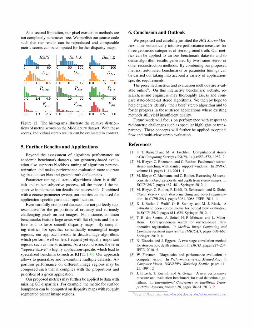
As a further experiment, we compute RMS scores oneach pixel subset of the metrics in order to separately testthe influence of our subset selection and of the metric func-tions applied to these sets. Rankings based on the subsetRMS scores are more similar to those defined by our metricsyet not identical5. We conclude that it is the combination ofsubset selection and metric function that makes our metricsspecific about their meaning. This is nicely illustrated bythe stereo results in Figure 5. Understandably, the RMS ismore specific about fine structure performance when beingapplied only to pixels at fine structures. Yet, the expressive-ness of metrics which incorporate spatial pixel distributionssuch as Ffrag cannot be achieved by the RMS metric.

Figure 10: RMS scores on the Jadeplant image are morecorrelated with BadPix than with our more specific metrics.(Algorithms at the lower left corner perform best).

Bad1.0 Bad4.0 Dfat Dthin Dfuz Fpor Ffrag Ffat Pbump Pdist Pmis

RMS 0.14 0.26 0.04 0.08 0.71 0.00 0.00 0.01 0.14 0.04 0.25

Bad1.0 - 0.66 0.14 0.05 0.03 0.05 0.07 0.35 0.06 0.10 0.26

Dfat 0.14 0.35 - 0.03 0.00 0.07 0.12 0.73 0.10 0.10 0.07

Fpor 0.05 0.06 0.07 0.01 0.00 - 0.62 0.13 0.09 0.02 0.00

Pbump 0.06 0.27 0.10 0.05 0.14 0.09 0.00 0.02 - 0.68 0.61

Figure 11: The coefficient of determination for linear fitsbetween scores across images and algorithms is very lowfor most pairs of metrics. The pairs (Bad1.0, Bad4.0) and(Dfat, Ffat) seem to be correlated on the Middlebury data.

4.5. Limitations

We identified two limitations of our proposed evaluationframework. First, our metrics are not homogenously nor-malized. Just like for the RMS, this is not an issue by it-self. Yet, in combination, the different ranges make it diffi-cult to get a good grasp of the relative differences betweenalgorithms across multiple metrics. To address this issue,we provide heuristic score distributions in Figure 12. Withthese histograms, individual metric scores can be put in con-text when assessing algorithm performance. As a furthersolution, our metrics could be rewritten to denote respec-tive percentages of bad pixels, e.g. the percentage of surfacenormals which are off by more than 5.

5Quantitative results on all images and algorithms are provided in Sec-tion 3.2. and the second column in Figure 6 of the supplemental material.

As a second limitation, our pixel extraction methods arenot completely parameter-free. We publish our source codesuch that our results can be reproduced and comparablemetric scores can be computed for further disparity maps.

Figure 12: The histograms illustrate the relative distribu-tions of metric scores on the Middlebury dataset. With thesescores, individual stereo results can be evaluated in context.

5. Further Benefits and ApplicationsBeyond the assessment of algorithm performance on

academic benchmark datasets, our geometry-based evalu-ation also supports blackbox tuning of algorithm parame-terization and makes performance evaluation more tolerantagainst dataset bias and ground truth deficiencies.

Parameter tuning of stereo algorithms often is a diffi-cult and rather subjective process, all the more if the re-spective implementation details are inaccessible. Combinedwith a coarse parameter sweep, our metrics can be used forapplication-specific parameter optimization.

Even carefully composed datasets are not perfectly rep-resentative for the proportions of ordinary and variouslychallenging pixels on test images. For instance, commonbenchmarks feature large areas with flat objects and there-fore tend to favor smooth disparity maps. By comput-ing metrics for specific, semantically meaningful imageregions, our approach avoids to disadvantage algorithmswhich perform well on less frequent yet equally importantregions such as fine structures. As a second issue, the term“representative” is highly application-specific which lead tospecialized benchmarks such as KITTI [10]. Our approachallows to generalize and re-combine multiple datasets. Al-gorithm performance on different image regions may becomposed such that it complies with the proportions andpriorities of a given application.

Our proposed metrics may further be applied to data withmissing GT disparities. For example, the metric for surfacebumpiness can be computed on disparity maps with roughlysegmented planar image regions.

6. Conclusion and OutlookWe proposed and carefully justified the HCI Stereo Met-

rics: nine semantically intuitive performance measures forthree geometric categories of stereo ground truth. Our met-rics can be applied to various benchmark datasets and todense algorithm results generated by two-frame stereo orother reconstruction methods. By combining our proposedmetrics, automated benchmarks or parameter tunings canbe carried out taking into account a variety of application-specific requirements.

The presented metrics and evaluation methods are avail-able online6. On this interactive benchmark website, re-searchers and engineers may thoroughly assess and com-pare state-of-the-art stereo algorithms. We thereby hope tohelp engineers identify “their best” stereo algorithm and tofoster progress in those stereo applications where existingmethods still yield insufficient quality.

Future work will focus on performance with respect toradiometric challenges such as specular highlights or trans-parency. These concepts will further be applied to opticalflow and multi-view stereo evaluation.

References[1] S. T. Barnard and M. A. Fischler. Computational stereo.

ACM Computing Surveys (CSUR), 14(4):553–572, 1982. 2[2] M. Bleyer, C. Rhemann, and C. Rother. Patchmatch stereo-

stereo matching with slanted support windows. In BMVC,volume 11, pages 1–11, 2011. 1

[3] M. Bleyer, C. Rhemann, and C. Rother. Extracting 3d scene-consistent object proposals and depth from stereo images. InECCV 2012, pages 467–481. Springer, 2012. 1

[4] M. Bleyer, C. Rother, P. Kohli, D. Scharstein, and S. Sinha.Object stereo - joint stereo matching and object segmenta-tion. In CVPR 2011, pages 3081–3088. IEEE, 2011. 1

[5] D. J. Butler, J. Wulff, G. B. Stanley, and M. J. Black. Anaturalistic open source movie for optical flow evaluation.In ECCV 2012, pages 611–625. Springer, 2012. 1

[6] T. R. dos Santos, A. Seitel, H.-P. Meinzer, and L. Maier-Hein. Correspondences search for surface-based intra-operative registration. In Medical Image Computing andComputer-Assisted Intervention (MICCAI), pages 660–667.Springer, 2010. 6

[7] N. Einecke and J. Eggert. A two-stage correlation methodfor stereoscopic depth estimation. In DICTA, pages 227–234.IEEE, 2010. 5

[8] W. Forstner. Diagnostics and performance evaluation incomputer vision. In Performance versus Methodology inComputer Vision, NSF/ARPA Workshop Seattle, pages 11–25, 1994. 2

[9] J. Fritsch, T. Kuehnl, and A. Geiger. A new performancemeasure and evaluation benchmark for road detection algo-rithms. In International Conference on Intelligent Trans-portation Systems, volume 28, pages 38–61, 2013. 2

6http://hci.iwr.uni-heidelberg.de/stereometrics

[10] A. Geiger, P. Lenz, and R. Urtasun. Are we ready for au-tonomous driving? the kitti vision benchmark suite. In CVPR2012, pages 3354–3361. IEEE, 2012. 1, 2, 8

[11] A. Geiger, M. Roser, and R. Urtasun. Efficient large-scalestereo matching. In ACCV 2010, pages 25–38. Springer,2011. 5

[12] F. Guney and A. Geiger. Displets: Resolving stereo ambigu-ities using object knowledge. In CVPR 2015, pages 4165–4175, 2015. 1

[13] R. M. Haralick. Performance characterization in computervision. In Computer Analysis of Images and Patterns, pages1–9. Springer, 1993. 2

[14] H. Hirschmuller. Stereo processing by semiglobal matchingand mutual information. PAMI, 30(2):328–341, 2008. 5

[15] H. Hirschmuller, P. R. Innocent, and J. Garibaldi. Real-timecorrelation-based stereo vision with reduced border errors.International Journal of Computer Vision, 47(1-3):229–246,2002. 3, 5

[16] L. Hong and G. Chen. Segment-based stereo matching usinggraph cuts. In CVPR 2004, volume 1, pages I–74. IEEE,2004. 1, 4

[17] C. G. Keller, M. Enzweiler, and D. M. Gavrila. A new bench-mark for stereo-based pedestrian detection. In Intelligent Ve-hicles Symposium, pages 691–696. IEEE, 2011. 2

[18] W. S. Kim, A. I. Ansar, R. D. Steele, and R. C. Steinke. Per-formance analysis and validation of a stereo vision system.In Systems, Man and Cybernetics, volume 2, pages 1409–1416. IEEE, 2005. 2

[19] D. Kondermann, S. Abraham, G. Brostow, W. Forstner,S. Gehrig, A. Imiya, B. Jahne, F. Klose, M. Magnor,H. Mayer, et al. On performance analysis of optical flowalgorithms. In Outdoor and Large-Scale Real-World SceneAnalysis, pages 329–355. Springer, 2012. 2

[20] D. Kondermann, R. Nair, S. Meister, W. Mischler,B. Gussefeld, K. Honauer, S. Hofmann, C. Brenner, andB. Jahne. Stereo ground truth with error bars. In ACCV 2014,pages 595–610. Springer International Publishing, 2015. 1

[21] J. Kostkova, J. Cech, and R. Sara. Dense stereomatchingalgorithm performance for view prediction and structure re-construction. In Image Analysis, pages 101–107. Springer,2003. 2

[22] J. Kowalczuk, E. T. Psota, and L. C. Perez. Real-time stereomatching on cuda using an iterative refinement methodfor adaptive support-weight correspondences. IEEE Trans-actions on Circuits and Systems for Video Technology,23(1):94–104, 2013. 5

[23] L. Maier-Hein, A. Groch, A. Bartoli, S. Bodenstedt, G. Bois-sonnat, P. L. Chang, N. T. Clancy, D. S. Elson, S. Haase,E. Heim, J. Hornegger, P. Jannin, H. Kenngott, T. Kilgus,B. Muller-Stich, D. Oladokun, S. Rohl, T. R. Dos Santos,H. P. Schlemmer, A. Seitel, S. Speidel, M. Wagner, andD. Stoyanov. Comparative validation of single-shot opticaltechniques for laparoscopic 3-d surface reconstruction. IEEETrans Med Imaging, 33(10):1913–1930, Oct 2014. 2, 6

[24] L. Maier-Hein, P. Mountney, A. Bartoli, H. Elhawary, D. El-son, A. Groch, A. Kolb, M. Rodrigues, J. Sorger, S. Spei-del, et al. Optical techniques for 3d surface reconstruction

in computer-assisted laparoscopic surgery. Medical imageanalysis, 17(8):974–996, 2013. 1, 2

[25] M. Maimone and S. A. Shafer. A taxonomy for stereocomputer vision experiments. In ECCV workshop on per-formance characteristics of vision algorithms, pages 59–79.Citeseer, 1996. 2

[26] R. Margolin, L. Zelnik-Manor, and A. Tal. How to evalu-ate foreground maps. In CVPR 2014, pages 248–255. IEEE,2014. 2

[27] N. Morales, G. Camellini, M. Felisa, P. Grisleri, and P. Zani.Performance analysis of stereo reconstruction algorithms. InProcs. IEEE Intl. Conf. on Intelligent Transportation Sys-tems, pages 1298–1303, 2013. 2

[28] M. G. Mozerov and J. van de Weijer. Accurate stereo match-ing by two-step energy minimization. IEEE Transactions onImage Processing, 24(3):1153–1163, 2015. 5

[29] J. Mulligan, V. Isler, and K. Daniilidis. Performance evalu-ation of stereo for tele-presence. In ICCV 2001, volume 2,pages 558–565. IEEE, 2001. 2

[30] B. Ozdemir, S. Aksoy, S. Eckert, M. Pesaresi, and D. Ehrlich.Performance measures for object detection evaluation. Pat-tern Recognition Letters, 31(10):1128–1137, 2010. 2

[31] D. Pfeiffer, S. Gehrig, and N. Schneider. Exploiting thepower of stereo confidences. In CVPR 2013, pages 297–304.IEEE, 2013. 1, 2

[32] S. Rohl, S. Bodenstedt, S. Suwelack, H. Kenngott, B. P.Muller-Stich, R. Dillmann, and S. Speidel. Dense GPU-enhanced surface reconstruction from stereo endoscopic im-ages for intraoperative registration. Med Phys, 39(3):1632–1645, 2012. 6

[33] D. Scharstein, H. Hirschmuller, Y. Kitajima, G. Krathwohl,N. Nesic, X. Wang, and P. Westling. High-resolution stereodatasets with subpixel-accurate ground truth. In PatternRecognition, pages 31–42. Springer, 2014. 1, 2

[34] D. Scharstein and R. Szeliski. A taxonomy and evaluation ofdense two-frame stereo correspondence algorithms. Interna-tional journal of computer vision, 47:7–42, 2002. 1, 2

[35] S. N. Sinha, D. Scharstein, and R. Szeliski. Efficient high-resolution stereo matching using local plane sweeps. InCVPR 2014, pages 1582–1589. IEEE, 2014. 4, 5

[36] C. Stentoumis, L. Grammatikopoulos, I. Kalisperakis, andG. Karras. On accurate dense stereo-matching using a localadaptive multi-cost approach. ISPRS Journal of Photogram-metry and Remote Sensing, 91:29–49, 2014. 5

[37] P. L. Venetianer and H. Deng. Performance evaluation of anintelligent video surveillance system–a case study. ComputerVision and Image Understanding, 114:1292–1302, 2010. 2

[38] W. A. Yasnoff, J. K. Mui, and J. W. Bacus. Error measuresfor scene segmentation. Pattern recognition, 9(4):217–231,1977. 2

[39] C. Zhang, Z. Li, R. Cai, H. Chao, and Y. Rui. As-rigid-as-possible stereo under second order smoothness priors. InECCV 2014, pages 112–126. Springer, 2014. 1, 4

[40] K. Zhang, J. Li, Y. Li, W. Hu, L. Sun, and S. Yang. Binarystereo matching. In ICPR 2012, pages 356–359. IEEE, 2012.5