THE GROWING IMPORTANCE OF THE ETF INDUSTRY - THE PROS …

FUNDAÇÃO GETÚLIO VARGAS

ESCOLA DE ECONOMIA DE EMPRESAS DE SÃO PAULO

EDOARDO CAMELA

THE GROWING IMPORTANCE OF THE ETF INDUSTRY - THE PROS AND

CONS OF PASSIVE MANAGEMENT

SÃO PAULO

2015

FUNDAÇÃO GETÚLIO VARGAS

ESCOLA DE ECONOMIA DE EMPRESAS DE SÃO PAULO

EDOARDO CAMELA



SÃO PAULO

2015

Dissertação apresentada à Escola de

Economia de Empresas de São Paulo da

Fundação Getúlio Vargas, como requisito

para obtenção do título de Mestre Profissional

em Economia.

Campo do Conhecimento:

International Master in Finance

Orientador Prof. Dr. Ricardo Rochman

Camela, Edoardo. The growing importance of the ETF industry – the pros and cons of passive management / Edoardo Camela. - 2015. 43 f. Orientador: Ricardo Rochman Dissertação (MPFE) - Escola de Economia de São Paulo. 1. Fundos de investimento. 2. Mercado financeiro. 3. Investimentos - Análise. 4. Custos de transação. I. Rochman, Ricardo. II. Dissertação (MPFE) - Escola de Economia de São Paulo. III. Título.

CDU 336.76

EDOARDO CAMELA



Dissertação apresentada à Escola de

Economia de Empresas de São Paulo da

Fundação Getúlio Vargas, como requisito

para obtenção do título de Mestre Profissional

em Economia.

Campo do Conhecimento:

International Master in Finance

Data de Aprovação:

___/___/____.

Banca Examinadora:

_________________________________

Prof. Dr. Ricardo Rochman

_________________________________

Prof. Dr. Melissa Prado

_________________________________

Prof. Dr. Martijn Boons

RESUMO

O objectivo deste projecto é a comparação entre os prós e contras de gestão passiva e

ativa através da realização de um estudo estatístico de várias estratégias através dos

Exchange-Traded Funds. Em particular, a análise vai passar pela estratégia mais passiva,

ou seja, buy and hold, para um grau diferente de active indexing management, tais como

rotações do sector e / ou classe de ativos com base no bottom-up, top-down e indicadores

técnicos. A análise mostra que as estratégias ativas, se forem devidamente aplicadas,

conseguem obter retornos ajustados ao risco substancialmente superiores quando

comparados com uma abordagem passiva, superando as questões de custos de transação

e diversificação que normalmente são reivindicadas por uma gestão passiva.

PALAVRAS CHAVE: ETF, gestão de portfolio, rotação de setores, rotação de classes

de ativos

ABSTRACT

The aim of this project is the comparison between the pros and cons of passive and active

management by conducting a statistical study of several strategies through Exchange-

Traded Funds. In particular, the examination will go through the most passive strategy,

namely buy & hold, to a different degree of active indexing management such as sector

and/or asset class rotations based on bottom-up, top-down and technical indicators. The

analysis show that active strategies, if properly implemented, obtain risk-adjusted returns

substantially higher than a passive approach, overcoming the issues of transaction costs

and diversification which are typically claimed by a passive management.

KEY WORDS: ETF, portfolio management, sector rotation, asset class rotation

TABLE OF FIGURES

Figure 1: Sectors’ cumulative returns over time .............................................................. 9

Figure 2: Correlation between sectors’ total return ........................................................ 14

Figure 3: Correlation between sectors’ excess return ..................................................... 14

Figure 4: S&P 500 and 7-10 years Treasury Bonds cumulative returns ........................ 15

Figure 5: Correlation between sectors and 7-10 years Treasury Bonds ......................... 15

Figure 6: Maximum and minimum 12-month volatility in sectors over time ................ 16

Figure 7: Maximum and minimum 12-month beta in sectors over time ........................ 17

Figure 8: Sector’s beta over the sample dates. ............................................................... 17

Figure 9: Buy and Hold graph and statistics .................................................................. 18

Figure 10: Equity and Bonds Buy and Hold graph and statistics ................................... 20

Figure 11: Rebalancing 60/40 graph and statistics ......................................................... 22

Figure 12: Technical strategy graph and statistics ......................................................... 26

Figure 13: Bottom-up strategy graph and statistics ........................................................ 29

Figure 14: Top-down strategy graph and statistics ......................................................... 34

Figure 15: Mixed strategy graph and statistics ............................................................... 35

Figure 16: Summary strategies’ statistics ....................................................................... 37

TABLE OF CONTENTS

1. Introduction to ETFs ................................................................................................. 9

2. Passive vs. Active Management .............................................................................. 10

3. Sectors and Asset Classes ETFs .............................................................................. 12

3.1. Data .................................................................................................................. 12

3.2. Statistics ........................................................................................................... 13

4. ETF Strategies ......................................................................................................... 17

4.1. Buy & Hold ...................................................................................................... 17

4.2. Rebalancing ..................................................................................................... 21

4.3. Technical .......................................................................................................... 23

4.4. Bottom-Up ....................................................................................................... 27

4.5. Top-Down ........................................................................................................ 30

4.6. Mixed Model .................................................................................................... 34

5. Conclusion ............................................................................................................... 37

References ...................................................................................................................... 40

9

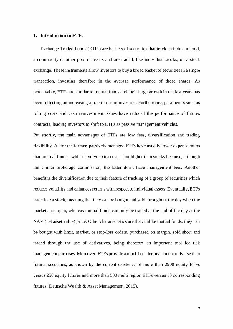
1. Introduction to ETFs

Exchange Traded Funds (ETFs) are baskets of securities that track an index, a bond,

a commodity or other pool of assets and are traded, like individual stocks, on a stock

exchange. These instruments allow investors to buy a broad basket of securities in a single

transaction, investing therefore in the average performance of those shares. As

perceivable, ETFs are similar to mutual funds and their large growth in the last years has

been reflecting an increasing attraction from investors. Furthermore, parameters such as

rolling costs and cash reinvestment issues have reduced the performance of futures

contracts, leading investors to shift to ETFs as passive management vehicles.

Put shortly, the main advantages of ETFs are low fees, diversification and trading

flexibility. As for the former, passively managed ETFs have usually lower expense ratios

than mutual funds - which involve extra costs - but higher than stocks because, although

the similar brokerage commission, the latter don’t have management fees. Another

benefit is the diversification due to their feature of tracking of a group of securities which

reduces volatility and enhances returns with respect to individual assets. Eventually, ETFs

trade like a stock, meaning that they can be bought and sold throughout the day when the

markets are open, whereas mutual funds can only be traded at the end of the day at the

NAV (net asset value) price. Other characteristics are that, unlike mutual funds, they can

be bought with limit, market, or stop-loss orders, purchased on margin, sold short and

traded through the use of derivatives, being therefore an important tool for risk

management purposes. Moreover, ETFs provide a much broader investment universe than

futures securities, as shown by the current existence of more than 2900 equity ETFs

versus 250 equity futures and more than 500 multi region ETFs versus 13 corresponding

futures (Deutsche Wealth & Asset Management. 2015).

10

Nevertheless, there might also be some drawbacks in the use of Exchange-Traded Funds,

in particular regarding liquidity and tracking error. As a matter of fact, the more

specialized, the higher the probability of large bid-ask spread of an ETF. These illiquid

ETFs, which are traded in low volumes, lead to problems when trying to close a position

which may not ensure the price desired. Moreover, as mentioned before, ETFs track the

performance of the underlying index, but sometimes managers may not succeed in that.

This tracking error can be a cost for the investors, which may see its performance

deviating from what it was supposed to be. Nevertheless, in these cases, arbitrage

opportunities arise and should restore the equilibrium price.

Other types of ETFs, which will not be included in the project analysis, are the leveraged,

the inverse and the active managed ones. Leveraged ETFs double or triple the

performance of the underlying asset by using derivatives and debt instruments as well as

inverse ETFs which replicate the opposite performance of the underlying securities.

Actively managed ETFs, as the name says, try to outperform its benchmark rather than to

replicate its performance.

2. Passive vs. Active Management

As previously mentioned, ETFs are mostly used for matching a determined index and

for this reason they are widely adopted for passive management purposes. Passive

strategies don’t involve any type of market forecasting and are only aimed at transaction

costs reduction and diversification, thereby enhancing returns and reducing volatility

(Ferri, 2010) when compared to the single stocks.

11

This approach is opposed to an active management, used by most mutual funds, where

the main goal is the outperformance of the market. Usually, active management

supporters claim that passive strategies are not able to minimize risk in the short-term,

especially during bear markets, and contrast the main principles of investing. As a matter

of fact, passive strategies have some limitations that may significantly disperse value over

time, such as long-term investing in indexes which, being mostly market capitalization

weighted, increase the weight of best performing stocks and decrease the weight of the

least performing ones, going against the investing philosophy of buying low and selling

high. Another example is the lack of macro and fundamental analysis, which leads

investors to buy a group of stocks without taking into account their valuation and the risk

in the economy. Furthermore, it is worth to note that a passive management might be

profitable only in case there are active managers that, by making proper valuations, push

the securities prices to their fair value. Therefore, if everyone goes passive there would

not be equilibrium in the stock market, whose inefficiency will lead active managers to

outperform the counterparts. On the other hand, the main criticism to the active

management is that on average it underperforms the benchmark after fees (Ferri, 2010).

Therefore, active strategies have the opportunity of outperforming the market but higher

transaction costs and wrong analysis may result in lower return than the benchmark. On

the other side, passive strategies imply low expenses but don’t exploit investment

opportunities which may potentially outperform the benchmark.

The solution to this debate might be the use of Exchange-Traded Funds as a tool for an

active index investing (Schoenfeld, 2004): this approach actively allocates securities on

the basis of the portfolio manager’s view by taking advantage of passive instruments

http://www.nasdaq.com/investing/mutual-funds.aspx

12

which ensure diversification, risk control and transaction costs minimization, leading to

a potential outperformance over a passive ETF strategy.

3. Sectors and Asset Classes ETFs

3.1. Data

To investigate the pros and cons of passive and active index approaches, a comparison

between buy and hold, rebalancing, bottom-up, top-down, technical and mixed strategies

will be undertaken. In particular, the active strategies will be based on sector and asset

class rotation. The reason to consider sector ETFs is due to the increasing importance of

industry effects, more related to business cycles, over country effects which are

diminishing over time as a consequence of larger financial market integration and

business globalization, as explained in Phylaktis et al (2002) and Weiss et al (2006).

The reason to consider asset class rotation, in this case between equity and bonds, is

related to their different sensibilities to business cycles, which will allow the investor

“leveraging” the equity performance during bull markets and limiting drawdowns during

crashes (Faber, 2013). For this purpose, nine broad US sectors and two broad asset classes

ETFs are considered. These nine sectors, belonging to S&P, are: Consumer Discretionary

(XLY US), Consumer Staples (XLP US), Energy (XLE US), Financials (XLF US),

Health Care (XLV US), Basic Materials (XLB US), Technology (XLK US), Utilities

(XLU US) and Industrials (XLI US) sectors from the SPDR family. The two asset classes

are: Equity, represented by the market index S&P 500 (IVV US) and Bonds, referred to

the 7-10 years Treasury Bonds (IEF US). The reason for the test to be undertaken on US

securities is their long-standing feature, data ranging from around 2003 to 2015, since

European sectors ETFs have been established some years later. Moreover, to make the

13

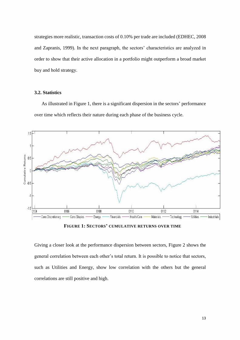
strategies more realistic, transaction costs of 0.10% per trade are included (EDHEC, 2008

and Zapranis, 1999). In the next paragraph, the sectors’ characteristics are analyzed in

order to show that their active allocation in a portfolio might outperform a broad market

buy and hold strategy.

3.2. Statistics

As illustrated in Figure 1, there is a significant dispersion in the sectors’ performance

over time which reflects their nature during each phase of the business cycle.

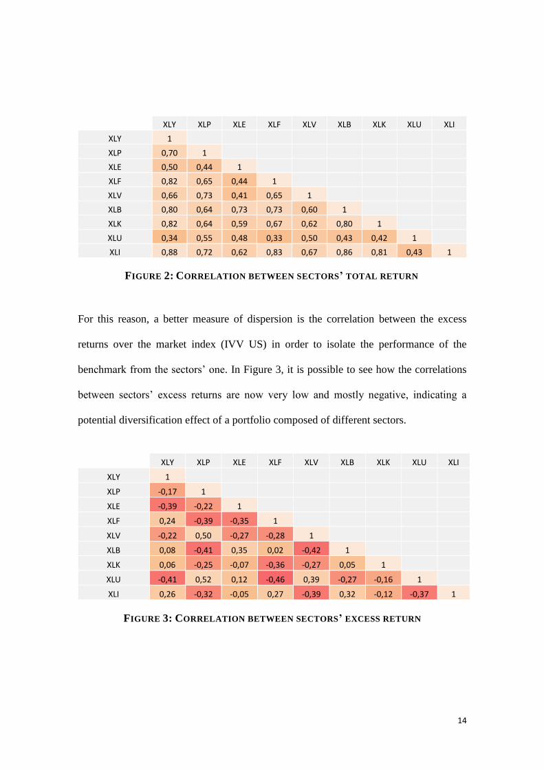
Giving a closer look at the performance dispersion between sectors, Figure 2 shows the

general correlation between each other’s total return. It is possible to notice that sectors,

such as Utilities and Energy, show low correlation with the others but the general

correlations are still positive and high.

FIGURE 1: SECTORS’ CUMULATIVE RETURNS OVER TIME

14

XLY XLP XLE XLF XLV XLB XLK XLU XLI

XLY 1

XLP 0,70 1

XLE 0,50 0,44 1

XLF 0,82 0,65 0,44 1

XLV 0,66 0,73 0,41 0,65 1

XLB 0,80 0,64 0,73 0,73 0,60 1

XLK 0,82 0,64 0,59 0,67 0,62 0,80 1

XLU 0,34 0,55 0,48 0,33 0,50 0,43 0,42 1

XLI 0,88 0,72 0,62 0,83 0,67 0,86 0,81 0,43 1

For this reason, a better measure of dispersion is the correlation between the excess

returns over the market index (IVV US) in order to isolate the performance of the

benchmark from the sectors’ one. In Figure 3, it is possible to see how the correlations

between sectors’ excess returns are now very low and mostly negative, indicating a

potential diversification effect of a portfolio composed of different sectors.


XLY 1

XLP -0,17 1

XLE -0,39 -0,22 1

XLF 0,24 -0,39 -0,35 1

XLV -0,22 0,50 -0,27 -0,28 1

XLB 0,08 -0,41 0,35 0,02 -0,42 1

XLK 0,06 -0,25 -0,07 -0,36 -0,27 0,05 1

XLU -0,41 0,52 0,12 -0,46 0,39 -0,27 -0,16 1

XLI 0,26 -0,32 -0,05 0,27 -0,39 0,32 -0,12 -0,37 1

FIGURE 3: CORRELATION BETWEEN SECTORS’ EXCESS RETURN

FIGURE 2: CORRELATION BETWEEN SECTORS’ TOTAL RETURN

15

The allocation of a portfolio can’t be limited to only equity. Although the low correlation

between excess returns, all the sectors are exposed to market crashes with a different

degree. To further improve the strategies it is thus necessary diversifying into other asset

classes such as bonds, whose performance is uncorrelated to equity (Figure 4).

In Figure 5 it is worth to notice that the sectors with highest correlation with the 10 year

Treasury Bond are the so called “Defensives”, namely Consumer Staples (XLP), Health

Care (XLV) and particularly Utilities (XLU).


IEF -0,21 -0,02 -0,31 -0,21 -0,09 -0,27 -0,29 0,14 -0,24

As a matter of fact, over the years empirical studies have shown that sectors can be

classified on the basis of their behavior during different stages of business cycles, where

Cyclicals and Sensitives (Consumer Discretionary, Technology, Financials, Energy,

FIGURE 4: S&P 500 AND 7-10 YEARS TREASURY BONDS CUMULATIVE RETURNS

FIGURE 5: CORRELATION BETWEEN SECTORS AND 7-10 YEARS TREASURY BONDS

16

Materials and Industrials) tend to perform better during early and late bull markets, and

indeed Defensives (Consumer Staples, Health Care and Utilities) during bear markets.

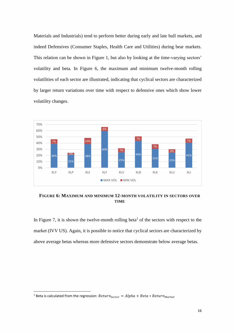
This relation can be shown in Figure 1, but also by looking at the time-varying sectors’

volatility and beta. In Figure 6, the maximum and minimum twelve-month rolling

volatilities of each sector are illustrated, indicating that cyclical sectors are characterized

by larger return variations over time with respect to defensive ones which show lower

volatility changes.

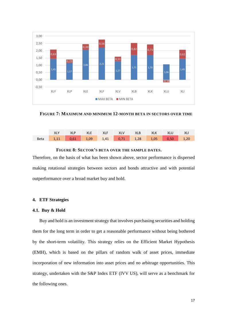
In Figure 7, it is shown the twelve-month rolling beta1 of the sectors with respect to the

market (IVV US). Again, it is possible to notice that cyclical sectors are characterized by

above average betas whereas more defensive sectors demonstrate below average betas.

1 Beta is calculated from the regression: 𝑅𝑒𝑡𝑢𝑟𝑛𝑆𝑒𝑐𝑡𝑜𝑟 = 𝐴𝑙𝑝ℎ𝑎 + 𝐵𝑒𝑡𝑎 ∗ 𝑅𝑒𝑡𝑢𝑟𝑛𝑀𝑎𝑟𝑘𝑒𝑡

39%

21%

38%

60%

25%

44%31%

25%

41%

7%

3%

10%

6%

7%

7%

7%

6%

7%

0%

10%

20%

30%

40%

50%

60%

70%


MAX VOL MIN VOL

FIGURE 6: MAXIMUM AND MINIMUM 12-MONTH VOLATILITY IN SECTORS OVER

TIME

17


Beta 1,11 0,61 1,09 1,41 0,71 1,28 1,05 0,50 1,20

Therefore, on the basis of what has been shown above, sector performance is dispersed

making rotational strategies between sectors and bonds attractive and with potential

outperformance over a broad market buy and hold.

4. ETF Strategies

4.1. Buy & Hold

Buy and hold is an investment strategy that involves purchasing securities and holding

them for the long term in order to get a reasonable performance without being bothered

by the short-term volatility. This strategy relies on the Efficient Market Hypothesis

(EMH), which is based on the pillars of random walk of asset prices, immediate

incorporation of new information into asset prices and no arbitrage opportunities. This

strategy, undertaken with the S&P Index ETF (IVV US), will serve as a benchmark for

the following ones.

1,451,17

2,06 2,21

1,271,71 1,70

1,061,45

0,63

0,23

0,390,56

0,31

0,82 0,73

-0,18

0,61

-0,50

0,00

0,50

1,00

1,50

2,00

2,50

3,00


MAX BETA MIN BETA

FIGURE 7: MAXIMUM AND MINIMUM 12-MONTH BETA IN SECTORS OVER TIME

FIGURE 8: SECTOR’S BETA OVER THE SAMPLE DATES.

18

2

Strengths:

2 Start DD: starting month max DD. Recovery DD: recovery month max DD.

Strategy

Securities

Parameters

Description

Run dates

Average Return 5,74% Skew -1,03 Max Drawdown 74%

Standard Deviation 14,56% Kurtosis 5,65 Start DD 65

Info Sharpe 0,39 Max 10,12% Recovery DD 114

Positive Months 61% Q3 3,10% Time recovery 49

Negative Months 39% Median 1,24% Alpha 0

Q1 -1,92% Beta 1

Min -18,19% Info Ratio NaN

Statistics

Buy & Hold

S&P ETF (IVV US)

n.a.

Long IVV US and hold over time

2004-2015

FIGURE 9: BUY AND HOLD GRAPH AND STATISTICS

19

The buy-and-hold strategy allows minimizing the transaction costs by holding securities

for long term horizons thereby trading less frequently than other approaches. The cost

minimization will theoretically increase the overall return of the investment portfolio.

Moreover, the broad diversification allows the strategy to average the returns of different

sectors. By being invested 100% in equity it immediately captures the fast recovery after

crisis.

Weaknesses:

The strategy presents an annualized return of 5.74% versus an annualized volatility of

14.56%, resulting in an Info Sharpe 3 of 0.39 which is quite lower than the risk-adjusted

performance of the approaches that will follow. Moreover, a Buy & Hold strategy can’t

avoid crashes, such as in 2009, where the maximum drawdown was 74% - driven by a

minimum monthly return of -18.19% - which has been recovered after 49 months (more

than four years). Therefore, confirming the findings in Ang (2014), an only-equity buy &

hold is not optimal for a long-horizon investor: it is a single and static investment decision

where the investor selects an initial portfolio allocation without rebalancing through time,

leading him to be less exposed to bull and more exposed to bear markets with respect to

a more active strategy. Therefore, a determined degree of active index management might

overcome the passive approach weaknesses by exploiting potential outperforming

opportunities in both bull and bear markets.

3 Info Sharpe =

𝑟𝑖

𝜎𝑖

20

Before heading to active strategies, a more diversified passive approach might be buying

and holding the market index (IVV US) and the Treasury Bonds (IEF US) with an initial

allocation of 60/40.

Strategy

Securities

Parameters

Description

Run dates





Negative Months 40% Median 0,83% Alpha -0,12%

Q1 -1,14% Beta 0,59

Min -10,93% Info Ratio -0,02

Statistics

Buy & Hold E60 + B40

S&P ETF (IVV US), IEF US

n.a.

Long 60% IVV US and 40% IEF US and hold over time

2004-2015

FIGURE 10: EQUITY AND BONDS BUY AND HOLD GRAPH AND STATISTICS

21

In this case the benefits of holding bonds is clear: it reduces the maximum drawdown to

39%, the time of recovery (36 months) and the overall portfolio volatility. The Info

Sharpe is therefore enhanced to 0.62 versus the 0.39 of the full equity long-only. The only

remarks are: the strategy takes advantage of the recent bond bull market (which might

end in the future and ruin the performance) and the average annual return is only 5.62%.

4.2. Rebalancing

Rebalancing is the process of periodically restoring a predetermined target allocation

with the goal of risk minimization rather than return maximization. Supporters of this

strategy have demonstrated through empirical studies that the main contributor to a long-

horizon investment performance is the asset allocation (Beebower, 1991), thus,

considering variation in the portfolio composition over time, the fund needs to be

periodically rebalanced back to the original weights. This investment strategy is counter-

cyclical and can be explained with the most famous type of rebalancing which involves

equity and bonds: when stocks outperform they have a weight higher than originally

making their sale optimal, whereas when they underperform they need to be purchased

again to restore the target exposure. The reason behind is simple: low-volatile assets such

as bonds tend to obtain low returns whereas high-volatile ones, such as equity, tend to

obtain higher returns. Consequently, the faster growth of high-volatile assets weight in

the portfolio with respect to low-volatile ones will make essential for an investor to

undertake a rebalancing strategy rather than a basic diversified portfolio which instead

will become less diversified and more risky over time.

Therefore, rebalancing requires buying assets that have underperformed and selling assets

that have outperformed, reflecting its contrarian nature. For this reason, it can also be seen

22

as a type of value investing strategy which involves buying assets that had negative

returns but with higher future expected returns, and vice versa.

Strategy

Securities

Parameters

Description

Run dates





Negative Months 43% Median 0,46% Alpha -2,73%

Q1 -1,08% Beta 0,55

Min -11,50% Info Ratio -0,39

Statistics

Rebalancing 60/40

S&P ETF (IVV US), 10Y Treasury Bond ETF (IEF US)

n.a.

Rebalance IVV US to 60% and IEF US to 40% of the portfolio each

month.

2004-2015

FIGURE 11: REBALANCING 60/40 GRAPH AND STATISTICS

23

Strengths:

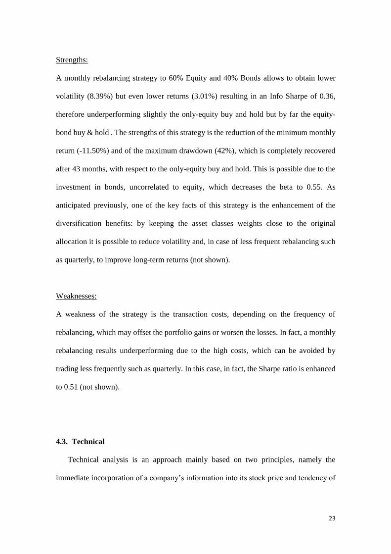
A monthly rebalancing strategy to 60% Equity and 40% Bonds allows to obtain lower

volatility (8.39%) but even lower returns (3.01%) resulting in an Info Sharpe of 0.36,

therefore underperforming slightly the only-equity buy and hold but by far the equity-

bond buy & hold . The strengths of this strategy is the reduction of the minimum monthly

return (-11.50%) and of the maximum drawdown (42%), which is completely recovered

after 43 months, with respect to the only-equity buy and hold. This is possible due to the

investment in bonds, uncorrelated to equity, which decreases the beta to 0.55. As

anticipated previously, one of the key facts of this strategy is the enhancement of the

diversification benefits: by keeping the asset classes weights close to the original

allocation it is possible to reduce volatility and, in case of less frequent rebalancing such

as quarterly, to improve long-term returns (not shown).

Weaknesses:

A weakness of the strategy is the transaction costs, depending on the frequency of

rebalancing, which may offset the portfolio gains or worsen the losses. In fact, a monthly

rebalancing results underperforming due to the high costs, which can be avoided by

trading less frequently such as quarterly. In this case, in fact, the Sharpe ratio is enhanced

to 0.51 (not shown).

4.3. Technical

Technical analysis is an approach mainly based on two principles, namely the

immediate incorporation of a company’s information into its stock price and tendency of

24

prices to move in trends. Contrarily to bottom-up, the technician doesn’t care about the

security fundamental information believing that it would be already anticipated by

investors who will create a trend. Fundamental information is therefore considered only

a distraction. The movement of the price – the price action - is the only powerful factor

that is needed to invest: as a matter of fact, they react to a market’s movement rather than

trying to predict its direction, giving them the ability of not getting emotionally involved

with the trades. This is therefore the essence of this approach: markets behave always the

same, with uptrends, downtrends and sideways which makes impossible to forecast a

changing direction but rather favoring the adaptation to it by following the trend. There

have been various studies about the existence of trends and momentum such as herding,

anchoring and underreaction, overreaction and disposition effect. The former regards the

investors’ behavior of following the crowd in case of a price movement, as shown in

numerous papers such as Welch et al (1992) and Grinblatt et al (1995). For instance, in

case of a sustained increase in a stock price, the majority of investors will start buying it

thereby boosting the price further, making it a self-fulfilling strategy. Moreover, investors

may anchor their ideas on past data thereby slowly reacting to news in the short-term

(Meub and Proeger, 2014), which consequently leads to an overreaction over longer

periods as the news are confirmed (Barberis et al, 1998). Lastly, the disposition effect

(Statman et al, 1985 and Grinblatt et al, 2005), namely the propensity to keep holding

winners and to sell losers too early, causes asset prices to not variate immediately

(Frazzini, 2006). The criticisms to this strategy regard their belief of repeatable patterns

of prices over time, indicating that past performance can predict the future performance

at a determined extent. Empirical studies show that this statement is false, since there is

slightly positive but very close to zero correlation between past and future price

25

movements. Again, the increasing notoriety of this strategy may cause a crowding out

thereby decreasing its effectiveness.

The factors that will be used in this strategy are a slight modification of the ones proposed

by Faber (2013) and Antonacci (2015): it will be used the ten-month trend following of

the benchmark as indication of equity bull and bear markets and the relative sector

momentum during the last ten months. The reason for this modification is that looking at

the direction of the market index rather than of each single sector allows averaging the

overall equity trend. Moreover, Faber and Antonacci’s strategies have become public and

widely used by investors which end up crowding them out, for this reason a slight

variation in the signal identification helps timing sectors and bond’s trends in a different

way. Once the path is individuated the investment will be done in either the three top ten-

month momentum sectors (Faber, 2013) or in the ten-years Treasury Bond.

26

Strategy

Securities

Parameters

Description

Run dates




Positive Months 63% Q3 3,01% Time rec 17

Negative Months 37% Median 0,93% Alpha 5,02%

Q1 -1,19% Beta 0,35

Min -8,82% Info Ratio 0,37

Statistics

Technical

10Y Treasury Bond ETF (IEF US), Sector ETFs, S&P ETF (IVV

US)

Trend Following 10 months IVV US, Sector Momentum 10 months

If IVV US price is above its 10 month Moving Average => long

Sectors ETFs with 10 months Price Momentum higher than the quantile

0.65 (i.e. top 3 sectors); Long IEF US otherwise.

2004-2015

FIGURE 12: TECHNICAL STRATEGY GRAPH AND STATISTICS

27

Strengths:

The strategy obtains an annualized return of 10.76% and annualized volatility of 10.77%,

resulting therefore in an Info Sharpe of 1 which is substantially higher than the buy &

hold. The main strength is the ability to capture the outperforming equity sectors during

bull markets and to avoid crashes by switching to bonds during bear markets (ex. 2009).

In fact, the maximum drawdown has only been 11% during the 2011-12 crisis and it was

recovered after only 17 months. Moreover, the strategy results to move less intensely than

the market (Beta=0.35) and to generate an alpha of 0.42%.

Weaknesses:

This method doesn’t allow to timing the beginning of a trend and its reversal, which

instead would be possible with a discretionary management. Moreover, keeping a

window of ten months might be too standardized since it should be fitted to the volatilities

of the sectors. On the other side, reducing or augmenting the window size will further

increase or reduce transaction costs.

4.4. Bottom-Up

The bottom-up investment approach is focused on the “micro” environment, namely

the analysis of securities’ fundamentals with the goal of picking the ones with greatest

profit potential. The bottom-up styles range from value investing – oriented to the

estimation of a company’s intrinsic value versus its trading price – to growth investing -

concentrated to the speed of earnings and/or revenues growth which might translate into

an increase in the stock price. As a matter of fact, these methods are based on the idea

that securities picking should be focused on the fundamentals, without considering the

28

short - term variations in the stock price. Being concentrated on the daily volatility of the

trading prices only confuses investors about what an asset is really worth, leading them

to undertake a wrong investment. For this reason, bottom-up investors believe that market

prices should only be used as a tool of investment timing, informing about whether a

bargain opportunity happens.

As for the factors, because of the diversity of sectors, it would be inefficient the use of

ratios as a selection tool. Therefore, the analysis will be undertaken by considering the

growth of profitability and efficiency measures, where ROA and EBIT together ended up

being the most significant. This is also consistent with the findings in Myers et al (2006),

where there is evidence of a relationship between earnings momentum and positive

abnormal returns, and in Turner et al (2011), where is found out that earnings momentum

is a persistent phenomenon and can lead to higher share prices. Return on Asset indicates

the ability of a company’s asset to generate profits, therefore an increasing ROA should

reflect an efficient use of the assets. It is a step behind the ROE, since it doesn’t take into

account the level of leverage. On the other side, EBIT rather than Net Income is used as

earnings indicator in order to eliminate the distortions caused by taxes and interest

expenses thereby facilitating the cross-sector comparison. Still consistent with Turner et

al (2011), the study is focused on past earnings rather than projected future earnings which

are usually overestimated because of optimistic views by analysts and conflict of

interests. Hence, an increasing EBIT indicates that the company has been growing in the

past and it is likely to continue doing so in the future. In summary, a positive twelve-

month change in these two measures indicates a strengthening of the sector, whereas a

negative one reflects a deteriorating performance thereby theoretically influencing the

market price.

https://www.boundless.com/finance/definition/leverage

29

Strategy

Securities

Parameters

Description

Run dates





Negative Months 36% Median 1,20% Alpha 4.82%

Q1 -1,28% Beta 0,94


Statistics

Bottom-up

10y Treasury Bond ETF (IEF US), Sector ETFs

12Months Momentum ROA, 12Months Momentum EBIT

Long Sectors with highest ROA 12M Momentum and highest EBIT 12M

Momentum (both>quantile 0.65); IEF US otherwise

2004-2015

FIGURE 13: BOTTOM-UP STRATEGY GRAPH AND STATISTICS

30

Strengths:

The strategy obtains an annualized return of 10.56% and annualized volatility of 17.26%,

resulting in an Info Sharpe of 0.61 which outperforms the buy & hold. It allows capturing

the sectors with the strongest profitability measures which might drive the market prices

in bull markets, for example by achieving a maximum monthly return of 16.76%. This is

reflected in the ability of capturing the fastest recovering sectors after crisis, which let the

drawdown to be offset after only 20 months.

Weaknesses:

A weakness of this investing approach is that it doesn’t consider the macro environment:

whatever the potential of a determined stock or sector, an economic downturn will

consequently affect the whole market thereby leading to potential losses, as shown by the

maximum drawdown of 50%, recovered after 20 months, and a very high Beta (0.94). In

fact, this type of investing, starting from the bottom, doesn’t consider the state of the

market, being therefore excessively exposed to equities rather than diversified with other

asset classes.

4.5. Top-Down

Top-Down strategy is an investment approach that is based on the analysis of the big

picture: through a detailed examination of market forces, a top-down manager tries to

understand cycles and trends which indicate the overall position of the economy and

consequently make the most appropriate trades. Therefore, after having analyzed the

macro factors the investor will identify the main themes and focus in individual securities.

One of the main beliefs of this strategy is the idea that picking the winner sector would

31

lead to picking the winner stocks, rather than departing from the companies’ fundamentals

analysis, method that require a relatively high degree of market inefficiency. Moreover,

a top-down strategy allows the investor to be flexible in both bull and bear markets by

shifting its portfolio allocation based on the general macro view. Another point in top-

down favor is the high degree of freedom: rather than focusing on only equity, like a

bottom-up manager would do, the global view investor will be able to rotate between

different asset classes and capturing their relative strength, improving thus the tactical

allocation of the portfolio. A criticism to the top-down investing is the degree of riskiness:

interpreting the macro environment is a hard task, therefore in case the manager’s forecast

is incorrect, the portfolio performance will be negatively impacted.

The strategy will be built on the PMI index, an indicator of the health of the manufacturing

sector, which is composed of five different factors namely manufacturing output,

inventory levels, new orders, supplier deliveries and the employment level. This index

influences the financial markets for several reasons such as being the first broad indicator

released each month and covering the cyclically sensitive manufacturing sector.

Moreover, it has been found out a very high correlation between PMI and US GDP. On

the basis of Harris et al (2004), the PMI is very accurate in the representation of the current

business cycle, leading the GDP at least one quarter ahead. In particular, the production

factor has been shown to be tightly correlated with personal income growth as well, which

affects both economy and financial markets. Therefore, a study of the PMI position might

be relevant for the allocation to determined industries (Crescenzi, 2009), which can be

divided into Cyclicals (Financials, Consumer Discretionary, Technology and Industrials),

Sensitives (Energy, Materials, Technology and Industrials), Defensives (Utilities, Health

Care, and Consumer Staples), rotating with bonds. To notice that Technology and

32

Industrials have been include in both early and late bull phases given their sensitivity to

both periods (Fidelity Investments, 2015 and Emsbo-Mattingly, 2014). In general, the

manufacturing sector is considered in expansion when the PMI is higher than 50 (i.e.

more firms are expanding activity than contracting activity), whereas when it is below 50

indicates a contraction. In this project the assessment of the business cycle will be done

by looking not only at the PMI level – i.e. above or below 50 points – but also at its

direction – i.e. above or below its moving average. In the latter, a moving average of six

months is used given the restrained PMI’s volatility in order to better timing the trend

variation. Accordingly to the PMI’s position and direction the economy is considered to

be divided in four stages:

1) When the PMI is higher than 50 and below its six-month moving average the

economy is considered strong but starting to deteriorate, phase that is here

specified as “early bear”. During this stage, long Defensives

2) When the PMI is lower than 50 and below its six-month moving average the

economy is considered weak and in recession, phase that is here specified as “late

bear”. During this stage, long ten-years Treasury Bonds ETF (IEF US)

3) When the PMI is lower than 50 and above its six-month moving average the

economy is considered weak but in recovery, phase that is here specified as “early

bull”. During this stage, long Cyclicals

4) When the PMI is higher than 50 and above its six-month moving average the

economy is considered strong and in expansion, phase that is here specified as

“late bull”. During this stage, long Sensitives

33

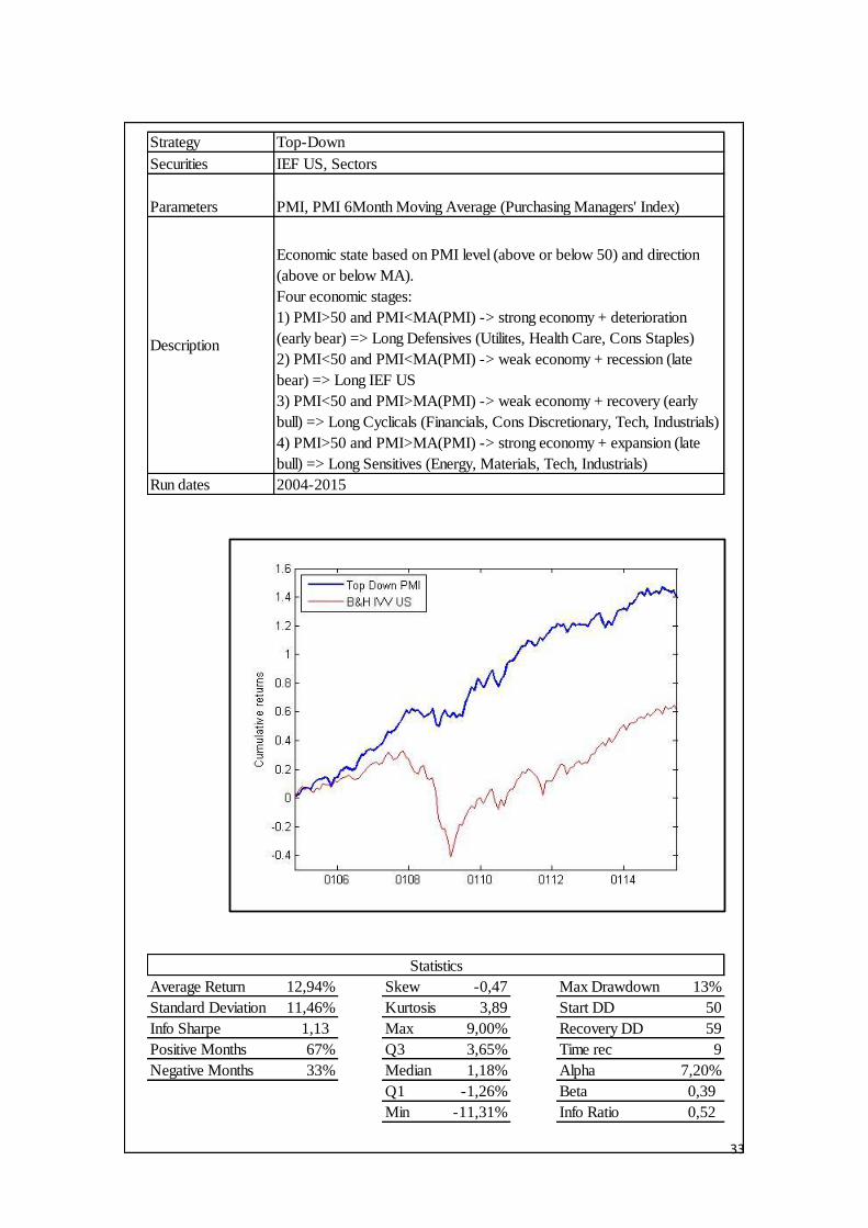
Strategy

Securities

Parameters

Description

Run dates




Positive Months 67% Q3 3,65% Time rec 9

Negative Months 33% Median 1,18% Alpha 7,20%

Q1 -1,26% Beta 0,39


Statistics

Top-Down

IEF US, Sectors

PMI, PMI 6Month Moving Average (Purchasing Managers' Index)

Economic state based on PMI level (above or below 50) and direction

(above or below MA).

Four economic stages:

1) PMI>50 and PMI<MA(PMI) -> strong economy + deterioration

(early bear) => Long Defensives (Utilites, Health Care, Cons Staples)

2) PMI<50 and PMI<MA(PMI) -> weak economy + recession (late

bear) => Long IEF US

3) PMI<50 and PMI>MA(PMI) -> weak economy + recovery (early

bull) => Long Cyclicals (Financials, Cons Discretionary, Tech, Industrials)

4) PMI>50 and PMI>MA(PMI) -> strong economy + expansion (late

bull) => Long Sensitives (Energy, Materials, Tech, Industrials)

2004-2015

34

Strengths:

The strategy obtains an annualized return of 12.94% and an annualized volatility of

11.46%, resulting in an Info Sharpe of 1.13, the top outperforming approach of this

project. By switching from Cyclical to Sensitive to Defensive sectors to bonds on the

basis of the PMI level and direction it allows capturing most of the market trends. The

maximum drawdown is thus only 13% and it is recovered after only 9 months, reflecting

the general ability of this strategy to be less intensely correlated with the market

(Beta=0.39) and to capture an alpha of 0.60%.

Weaknesses:

Sometimes the macro fundamentals may not be reflected in the market prices which are

mostly moved by investors’ irrationality. This explains the inability of this strategy to ride

the financial sector bubble before 2008 as other strategies do, but it allows predicting and

avoiding the following market crash.

4.6. Mixed Model

The mixed model tries to combine two different approaches – bottom-up and

technical, tested previously– in order to further improve the portfolio performance. The

top-down is excluded on purpose since it allocates the portfolio to predetermined sectors

in their potential outperforming phase, practice that would be in contrast with the

fundamentals and technical findings. In this case, the chosen factors are the twelve-month

rate of change in ROA and EBIT, as fundamentals, and the ten-month market moving

FIGURE 14: TOP-DOWN STRATEGY GRAPH AND STATISTICS

35

average and sectors’ price momentum, as technicals, with the goal of exploiting the

benefits of both approaches.

Strategy

Securities

Parameters

Description

Run dates



Info Sharpe 0,93 Max 13% Recovery DD 42

Positive Months 58% Q3 2% Time recovery 13

Negative Months 42% Median 1% Alpha 5,06%

Q1 -1% Beta 0,17

Min -11% Info Ratio 0,30

Statistics

Mixed: Bottom-up + Technical

IEF US, Sector ETFs

12M MOM ROA, 12M MOM PRICE, 12 MOM EBIT

If IVV US is above its 10M Moving Average => Long Sectors with highest ROA

12M Momentum (>quantile 0.65), highest and positive PRICE 10M MOM

(>quantile 0.65) and highest EBIT 12M Momentum (>quantile 0.65); IEF US

otherwise

2004-2015

FIGURE 15: MIXED STRATEGY GRAPH AND STATISTICS

36

Strengths:

The strategy allows to exploit both prices and fundamental momentum in the sectors. In

this way, it tries to improve the only-technical strategy by investing in sectors with

increasing profitability and efficiency and it tries to improve the only-bottom-up strategy

by looking at variations in price trends. The portfolio shifts from the sectors with strong

fundamentals and momentum during equity bull markets to bonds during equity bear

markets, achieving an annualized return of 10.81% (which is higher than the annualized

return in both technical and bottom-up strategy) and volatility of 11.67% (which

unfortunately is higher than the technical, even if quite lower than the bottom-up)

resulting in an Info Sharpe of 0.93. The strategy thus outperforms the buy and hold,

confirmed by a (daily) alpha of 0.42%, also from a the losses’ point of view: the maximum

drawdown is in fact only 16% - strangely not corresponding to neither the crisis in 2008

nor in 2012 – and it is recovered in 13 months. The strength of the strategy can also be

considered the relative market neutrality, reflected in a beta of only 0.17, due to the high

number of periods invested in bonds.

Weaknesses:

The volatility is still high due to the fundamental factors’ signals, even if smoothed by

the price momentum indicator, making this strategy underperforming the only-technical

one from the Info Sharpe point of view. The information ratio is only 0.09 compared to

the other strategies, meaning that the active returns are low for the risk taken. Moreover,

the strategy obtains 42% of negative months, which is even higher than the buy and hold

approach. Although the good Sharpe, the strategy might be not well working because of

the excessive filters for the equity signals which increases the number of periods invested

37

in bonds. In case bonds become less profitable over time there will be a probable

underperformance of this strategy.

5. Conclusion

In the last years the use of ETFs has been increasingly growing due to their advantages

over mutual funds and futures as a tool for passive management. In particular, the project

has the goal of showing that ETFs might be used as powerful instruments for an active

management approach, focusing on sector and asset class rotation, rather than for a

passive one. The active strategies undertaken are monthly rebalancing to 60% equity and

40% bonds, technical, bottom-up, top-down and mixed model. The analysis show that by

combining sector and asset class rotation it is possible to capture the strongest sectors

during an equity bull market and to substantially reduce losses by investing in bonds

during equity bear markets, making thus more efficient the use of ETFs for active

management rather than passive management purposes. In particular, it has been shown

that a strategy based on technical signals – ten-month price momentum and ten-month

trend following applied to the benchmark and sectors – allows capturing the strongest

sectors over time and moving to bonds in case of deteriorating performances, resulting in

an Info Sharpe of 1 which more than double the Info Sharpe of the benchmark buy and

hold (=0.39). The bottom-up strategy, by focusing on fundamentals, is oriented to capture

B&H Rebalancing Technical Bottom-up Top-down Mixed

Average Returns 5,74% 3,01% 10,76% 10,56% 12,94% 10,81%

Standard Deviation 14,56% 8,39% 10,77% 17,26% 11,46% 11,67%

Info Sharpe 0,39 0,36 1,00 0,61 1,13 0,93

Max DD 74% 42% 11% 50% 13% 16%

Months Recovery DD 49 43 17 20 9 13

FIGURE 16: SUMMARY STRATEGIES’ STATISTICS

38

the sectors with highest profitability and efficiency growth by looking at the rate of

change in their respective Return On Assets and EBIT. With this method it is possible to

achieve an Info Sharpe of 0.61, which again outperform a passive only-equity buy and

hold strategy, but the feature of focusing on fundamentals rather than prices and

macroeconomic state doesn’t allow the investor timing the bear markets and switching to

bonds. The top-down strategy, undertaken by looking at the PMI level and direction, is

revealed to be very efficient: in fact, it allows capturing the different phases of the

business cycle and the related outperforming sectors and asset classes, achieving an Info

Sharpe of 1.13. The only risk of this strategy might be the future distortion of the sector’s

performance during a determined moment of the cycle due to changes in endogenous

factors (ex: sectors’ regulations and technology) and in exogenous factors

(supply/demand). The mixed model, which excludes the top-down indicator (based on

predetermined sector choice), combines fundamental factors (ROA and EBIT) with

technical factors (trend following price momentum) in order to outperform the

benchmark. The strategy obtains an Info Sharpe of 0.93 by increasing the returns for the

level of volatility and an alpha of 0.42%. It is important to say that the goal of this paper

is not showing which type of active approach is the most efficient, since the choice and

the combination between factors is unlimited leading to large variations in the

performance, but it is rather demonstrating that the use of ETFs in active strategies, if

properly implemented, is greatly more profitable and less risky than in passive

management. This statement can be done not only from the Sharpe’s point of view but by

looking at the drawdowns: as shown in Figure 16: Summary strategies’ statistics, a

passive buy and hold strategy obtains a maximum drawdown of 74% which is recovered

after 49 months (more than four years) whereas active strategies allow to significantly

39

reduce the drawdowns and their time of recovery (ex. Max DD of 13% and recovered

after only 9 months for the top-down approach). Therefore, in the light of what the

analysis has shown, the theoretical “pros” of a passive management such as

diversification and absence of transaction costs are substantially overcome by the “pros”

of an active management.

To further investigate the potential outperformance of active over passive ETFs strategies

it is suggested to extend the research to analyze the effectiveness of the strategies in

different time periods – bull, bear and sideways – and to use super-sector ETFs in order

to additionally exploit the differences within each broad sector.

40

References

Ang, Andrew. 2014. Asset Management: A Systematic Approach to Factor Investing.

New York: Oxford University Press

Antonacci, Gary. 2015. Dual Momentum Investing. New York: McGraw-Hill Education

Barberis, Nicholas et al. 1998. “A Model of Investor Sentiment”. Journal of Financial

Economics

Beebower, Gilbert L. et al. 1991. “Determinants of Portfolio Performance II: An

Update”. Financial Analysts Journal

Beechey, Meredit, et al. 2000. “The Efficient Market Hypothesis: A survey”. Economic

Research Department Reserve Bank of Australia

Bodie, Zvi. 2014. Investments. New York: McGraw Hill Education

BlackRock. 2013. Exchange-Traded Products: Overview, Benefits and Myths.

BlackRock, Inc.

Covel, Michael W. 2009. Trend Following. New Jersey: Pearson Education

Clare, Andrew et al. 2013. “The Trend is Our Friend: Risk Parity, Momentum and Trend

Following in Global Asset Allocation”. CAMA Working Paper

Crescenzi, Anthony. 2009. Investing from the Top-Down. New York: McGraw-Hill

Deutsche Wealth & Asset Management. 2015. Can ETFs be a substitute for futures?

An intense debate, with changing dynamics. London

41

D’Hondt, Catherine et al. 2008. “Transaction Cost Analysis A-Z”. EDHEC Risk and

Asset Management Research Centre Publication

Emsbo-Mattingly, Lisa. 2014. “The Business Cycle Approach to Equity Sector

Investing”. Fidelity Investments Market Research

Faber, Mebane T. 2013. “A Quantitative Approach to Tactical Asset Allocation”.

Cambria Capital

Ferri, Richard A. 2008. The ETF Book: All you need to know about Exchange-Traded

Funds. Hobokonen: Wiley & Sons, Inc.

Ferri, Richard A. 2011. The Power of Passive Investing. New Jersey: Wiley & Sons,

Inc.

Fidelity Learning Center. 2015. The drawbacks of ETF.

Fidelity Investments. 2015. “Compare Sector Characteristics”

Franklin Templeton Investments. 2015. Beyond Bulls and Bears: Active Opportunities

in a Passive World. Franklin Templeton Distributors, Inc.

Frazzini, Andrea. 2006. “The Disposition Effect and Underreaction to News”. Journal

of Finance

FTSE International Limited. 2015. Why indexing matters. FTSE International Limited

Grinblatt, Mark et al. 1998. “Momentum Investment Strategies, Portfolio Performance

and Herding: A Study of Mutual Fund Behavior”. American Economic Review

42

Harris, Ethan S. 1991. “Tracking the Economy with the Purchasing Managers’ Index”.

FNRBY Quarterly Review

Harris, Matthew et al. 2004. “Using Manufacturing Surveys to Assess Economic

Conditions”. Federal Reserve Bank of Richmond, Economic Quarterly

Jacobsen, Brian J. et al. 2010. Market cycles and business cycles. Boston: Wells Fargo

Advantage Fund

Jaconetti, Colleen M. et al. 2010. “Best Practices for Portfolio Rebalancing”. Vanguard

Research

Koenig, Evan F. 2002. “Using the Purchasing Managers’ Index to Assess the Economy’s

Strength and the Likely Direction of Monetary Policy”. Federal Reserve Bank of Dallas

Economic and Financial Policy Review, Vol. 1, No. 6

Malkiel, Burton G. 1999. A Random Walk Down Wall Street. New York: W. W. Norton

& Company

Meub, Lukas et al. 2014. “An Experimental Study on Social Anchoring”. Working Paper

Myers, James N. 2006. “Earnings Momentum and Earnings Management”.

Phylaktis, Kate et al. 2002. “The Changing Roles of Industry and Country Effects in the

Global Equity Markets”.

Schoenfeld, Steven A. 2004. Active Index Investing. New Jersey: Wiley & Sons, Inc.

Smith Barney Citigroup. 2005. “The Art of Rebalancing”.

43

Statman, Meir et al. 1985. “The Disposition to Sell Winners Too Early and Ride Losers

Too Long: Theory and Evidence”. Journal of Finance

Threadneedle. 2010. Is Active management doomed? Threadneedle Thinks

Timo, Roberto. The pros and cons of Passive Management. Institute for Fiduciary

Education

Turner, Bob et al. 2011. “Yes, earnings do drive stock prices”. Turner Investments

Weiss, Richard et al. 2006. “The Rise of Sector Effects in Major Equity Markets”.

Financial Analysts Journal

Welch, Ivo et al. 1992. “A Theory of Fads, Fashion, Custom, and Cultural Change as

Informational Cascades”. Journal of Political Economy

Wild, Russel. 2007. Exchange-Traded Funds for Dummies. Indianapolis: Wiley

Publishing, Inc.

Zapranis, Achilleas et al. 1999. Principles of Neural Model Identification, Selection and

Adequacy. London: Springer-Verlag

Documents

THE GROWING IMPORTANCE OF THE ETF INDUSTRY - THE PROS …